CONVOLUTIONAL COMPACTION OF TEST RESPONSES

Janusz Rajski, Jerzy Tyszer*, Chen Wang, Sudhakar M. Reddy**

Mentor Graphics Corporation 8005 S.W. Boeckman Road

Wilsonville, OR 97070, USA

*Poznan University of Technology ul. Piotrowo 3a

60-965 Poznan, Poland

**University of Iowa ECE Department

Iowa City, IA 52242, USA

Abstract This paper introduces a finite memory compactor called convolutional compactor that provides compaction ratios of test responses in excess of 100x even for a very small number of outputs. This is combined with the capability to detect multiple errors, handling of unknown states, and the ability to diagnose failing scan cells directly from compacted responses. A convolutional compactor can be easily configured into a MISR that preserves most of these properties. Experimental results demonstrate the effi-ciency of compaction for several industrial circuits.

1. Introduction

The increasing body of experimental evidence shows that as semiconductor industry is moving to 0.13 micron tech-nology and beyond, it becomes necessary to use at-speed test and to target transition fault models to achieve ac-ceptable quality of test [1]. The adoption of at-speed test-ing and the corresponding fault models, combined with the omnipresent exponential increase in gate count, result in a growth of test data volume that is much faster than what is indicted by Moore’s law. In order to address the rapid increase in volume of test data a number of com-pression schemes have been developed [2], [8], [10], [15].

Detailed analysis of test cube profiles generated by ATPG tools for a wide range of integrated circuits indicates that in many cases, especially where there are no bus conten-tion issues, the average fill rate is well below 1% [10]. With such a very low fill rate it is possible to achieve compression of test stimuli well in excess of 100 times [15]. It is also well known that many designs produce unknown states (often denoted as X states) in test re-sponses, and it is too intrusive to remove them.

All test response compaction schemes, which have been proposed until now, belong to one of two classes.

Time (or infinite memory) compactors include polynomial division, counting based techniques, and check sum based methods [19], and all of them are typically used in built-in self-test (BIST) applications. The compaction is usually performed by linear finite state machines such as linear feedback shift registers (LFSRs), multiple input signature registers (MISRs), or cellular automata. A characteristic feature of these compactors is the infinite impulse re-sponse property. They are capable of compacting gigabits

of test response data into a small signature, typically 32-, 64-, or 128-bit long, achieving compaction ratios between 106 and 108. This is possible because an error, once in-jected into this type of a compactor, will remain there until another group of errors erases it in the rare case of aliasing. These schemes require that all values in test responses be known. An unknown state injected into an infinite impulse response compactor corrupts the signa-ture and renders the test useless. Fault diagnosis is also more complicated and it requires multiple passes with direct access to pre-compacted responses [19].

Space compactors, on the other hand, are combinational circuits, predominantly built of XOR networks to generate n test outputs from m primary outputs of the circuit under test (CUT), where n < m. They offer smaller compaction than the previous class of compactors but they can handle unknown states in responses without circuit modification. The first space only compaction scheme using error codes was proposed in [18]. It was then followed by many other compaction techniques [9], [11], [17], [19]. Some designs, including non-linear spatial compactors, were even cus-tomized for a given CUT and for a given test set to elimi-nate the aliasing phenomenon [3] - [6], [13], [14]. Re-cently, the X-Compact technique was proposed in [12] to handle simultaneous errors and unknown logic values, both arriving from multiple scan chains.

In this paper we introduce finite memory compactors called convolutional compactors – a completely new class of compaction schemes. These compactors have the char-acteristic of finite impulse response. They have been designed specifically for Embedded Deterministic Test (EDT) technology [15], [16] to handle the following re-quirements of high quality low cost manufacturing test:

• support of output response compaction with effective ratios in excess of 100 times,

• consistent properties for a whole range of configura-tions, starting from a single output,

• ability to detect errors of multiplicity 1, 2, 3, and any odd multiplicity with no aliasing,

• very low probability of aliasing (i.e., less than 10-6) of errors of even multiplicity starting from 4 and higher,

• ability to handle unknown states in test responses, • capability to perform diagnosis, i.e., identify failing

scan cells directly from the compacted responses.

ITC INTERNATIONAL TEST CONFERENCE Paper 29.3

7450-7803-8106-8/03 $17.00 Copyright 2003 IEEE

The paper is organized as follows. Section 2 describes architecture of a convolutional compactor. In section 3, error masking is discussed in the absence of unknown states. Section 4 extends the previous analysis to cases where quality of compaction can be compromised by unknown values. In Section 5, diagnostic capabilities of convolutional compaction are described. Section 6 intro-duces a convolutional MISR. To conclude, several ex-perimental results are presented in Section 7.

2. Convolutional compactor

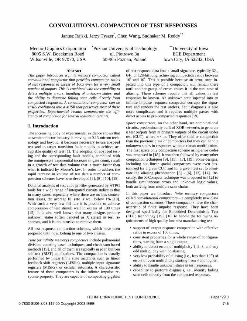
Figure 1 shows an example of a convolutional compactor with 16 inputs (observing 16 scan chain outputs), two outputs, and six memory elements – three per output. Although a detailed discussion of properties of convolu-tional compactors will follow in subsequent paragraphs, it is easy to recognize the following characteristics. Every scan cell error can reach memory elements and then out-puts in three possible ways. For instance, the scan chain no. 7 is connected to bits 1, 3, and 6 of the register. It can also be seen that the last memory element is driven, in addition to scan no. 7, by scan chains labeled as 4, 9, 10, 13, 15, and 16. In general, the spatial part of the compac-tor consists of M single-output XOR networks connected to the register by means of additional 2-input XOR gates interspersed between successive memory elements.

Fig. 1. Example of convolutional compactor

As can be seen, the compactor does have memory but no feedback. Consequently, any error or unknown state in-jected into the compactor is shifted out after at most three cycles. Due to fan-outs, every error may propagate to one or two outputs three times. No single X state can mask an error. No odd number of errors or two errors injected at the same time or in different time frames can mask each other completely. Also, single errors injected in each scan propagate to outputs in a different recognizable pattern. It is worth noting that if one increases the number of mem-ory elements from 6 to, say, 18, the number of scan chains that can be connected to the compactor, and can be still observed on two outputs goes up to 256.

1

Injector network

M

Scan chain outputs

Compactor outputs

…

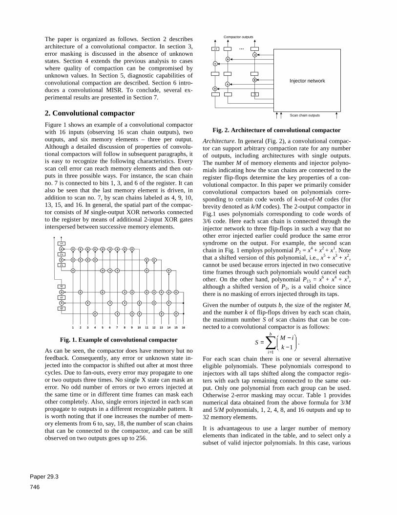
Fig. 2. Architecture of convolutional compactor

Architecture. In general (Fig. 2), a convolutional compac-tor can support arbitrary compaction rate for any number of outputs, including architectures with single outputs. The number M of memory elements and injector polyno-mials indicating how the scan chains are connected to the register flip-flops determine the key properties of a con-volutional compactor. In this paper we primarily consider convolutional compactors based on polynomials corre-sponding to certain code words of k-out-of-M codes (for brevity denoted as k/M codes). The 2-output compactor in Fig.1 uses polynomials corresponding to code words of 3/6 code. Here each scan chain is connected through the injector network to three flip-flops in such a way that no other error injected earlier could produce the same error syndrome on the output. For example, the second scan chain in Fig. 1 employs polynomial P2 = x4 + x2 + x1. Note that a shifted version of this polynomial, i.e., x5 + x3 + x2, cannot be used because errors injected in two consecutive time frames through such polynomials would cancel each other. On the other hand, polynomial P15 = x6 + x4 + x3, although a shifted version of P2, is a valid choice since there is no masking of errors injected through its taps.

Given the number of outputs b, the size of the register M, and the number k of flip-flops driven by each scan chain, the maximum number S of scan chains that can be con-nected to a convolutional compactor is as follows:

∑=

−−

=b

ik

iMS

11

.

For each scan chain there is one or several alternative eligible polynomials. These polynomials correspond to injectors with all taps shifted along the compactor regis-ters with each tap remaining connected to the same out-put. Only one polynomial from each group can be used. Otherwise 2-error masking may occur. Table 1 provides numerical data obtained from the above formula for 3/M and 5/M polynomials, 1, 2, 4, 8, and 16 outputs and up to 32 memory elements.

It is advantageous to use a larger number of memory elements than indicated in the table, and to select only a subset of valid injector polynomials. In this case, various

1 2 3 4 5 6 7 8 9 10 11 12 13 14 15 16

12

34

56

Paper 29.3

746

experimental results indicate that the best performance is achieved by choosing polynomials randomly rather than following their lexicographic order. From each group of alternative polynomials we select one, also at random. Both of the random selections help in balancing the XOR networks. They also provide a better distribution of mul-tiple errors and reduce masking of multiple even errors.

Table 1. The maximum number of observable scan chains in convolutional compactors

Outputs – 3/M polynomials

M 1 2 4 8 16

3 1 1

4 3 4 4

6 10 16 20

8 21 36 52 56

10 36 64 100 120

12 55 100 164 216

16 105 196 340 504 560

20 171 324 580 920 1136

24 253 484 884 1464 1968

28 351 676 1252 2136 3056 32 465 900 1684 2936 4400

Outputs – 5/M polynomials

M 1 2 4 8 16

6 5 6 6 8 35 50 56 56

10 126 196 246 252

12 330 540 736 792

16 1365 2366 3576 4312 4368 20 3876 6936 11136 14712 15504

24 8855 16170 27000 38136 42448 28 17550 32500 55776 82776 97488

32 31465 58870 103096 158872 197008

Table 2. The maximum number of scan chains in the X-Compact and convolutional compactors

Outputs X-C CC-3/16 CC-3/32

5 10 395 2035

6 20 440 2360

7 35 476 2660

8 56 504 2936

9 126 525 3189

10 252 540 3420

11 462 550 3630

12 792 556 3820

13 1716 559 3991

14 3432 560 4144

Table 2 shows a dramatic impact of the sequential part of a convolutional compactor on the maximum number of observable scan chains. For example, a compactor with 8 outputs can observe at most 56 scan chains in the X-Compact (X-C) scheme [12] with the resulting maximum

compaction of 7x. A convolutional compactor (CC) with 3/16 polynomials can observe up to 504 scan chains using 16 flip-flops, and 2936 scan chains connected to 32 flip-flops. The corresponding compaction ratios are 63x and 367x, respectively. This property makes the proposed scheme very well suited for a wide range of modular designs where each block may possess a separate compac-tor with a very small number of outputs while still provid-ing very high compaction ratios.

Synthesis. It is worth noting that the actual number of 2-input XOR gates used to implement the injector polyno-mials is usually much smaller than the upper bound S⋅ k, where S is the number of scan chains, and k is the number of flip-flops driven by each scan chain. For instance, factorization applied to a 2-output convolutional compac-tor employing 3/32 polynomials and supplied by 900 scan chains reduces the XOR gate count from the original value of 2668 to 1833. As a result, there are, on the aver-age, 57 XOR gates driving each compactor flip-flop. Alternatively, a delay introduced by the XOR tree logic is approximately equivalent to 6 XOR gates. The same compactor driven by 200 scan chains features, after fac-torization, 423 XOR gates rather than 568, and thus only 4-gate delay is introduced by the XOR tree logic.

3. Error masking in the absence of X states

In this section we analyze the masking properties of con-volutional compactors designed with k/M polynomials. We assume that each polynomial has the same odd num-ber of terms, i.e., 3, 5, 7, etc. The following properties define the capabilities of convolutional compactors.

Property 1: A convolutional compactor with k/M poly-nomials, for k = 3, 5, 7, … detects errors from one, two or any odd number of scan chains provided that all scan chains produce X-state free responses. The errors can be injected at the same time or at different shift cycles.

Since from each group of alternative polynomials we use only one, there are no shifted versions of injectors, and an effect of an error injected into the compactor cannot be erased by another error injected in the same or later cycle. Let k = 3. Then two errors can leave an error syndrome in the register that involves 2 bits – if the original errors overlap on 2 positions, 4 bits – if they overlap on one bit, or 6 bits – if they do not overlap. A third error injected from a scan chain can leave the number of affected regis-ters at 1, 3, 5, 7, or 9. A fourth error can set the number of affected registers at 0, 2, 4, 6, 8, 10, and 12. Clearly, 0 indicates 4-error masking. A similar reasoning applies to other odd values of fan-out size k.

As shown above, detection of errors of multiplicity 4 and higher even multiplicity is not guaranteed. To study the size of this problem, extensive experiments were con-ducted to measure the frequency of 4-error masking and

Paper 29.3

747

its dependence on the size of registers, the polynomials employed, and the time span of errors. Each measurement was done by conducting Monte Carlo simulations for at most 100 million error configurations. The following observations are drawn from the experimental results:

• compaction ratio has a marginal impact on the prob-ability of 4-error masking as shown in Table 3,

• for the same level of compaction, the number of compactor outputs has a marginal impact on 4-error masking (Table 3),

• polynomials with a greater number of terms perform better than those with a small number of terms; in particular Table 3 shows clear superiority of polyno-mials 5/M over 3/M ones,

• 4-error masking drops quickly with the increasing number of compactor flip-flops (see Table 4 – re-sults for M = 16 and 2 as well as 4 outputs were ob-tained for 196 and 340 scan chains, respectively, which are the maximum numbers of allowed scans; the same rule applies to results presented in Table 5),

• 4-error masking drops quickly with the increasing time span of errors; in all previous experiments errors were injected in the same cycle from scan chain out-puts; Table 5 shows experiments where errors are in-jected over some number of clock cycles defined as an error time span.

Table 3. 4-error masking for 20- and 32-bit registers

Register size / outputs C k

20/1 20/2 20/4 20/8 32/16 32/32

3 6.05e-5 6.77e-5 5.27e-5 4.05e-5 2.95e-6 2.74e-6 100x

5 4.35e-6 5.62e-6 5.30e-6 4.75e-6 3.00e-8 6.00e-8

3 4.78e-5 7.18e-5 5.79e-5 3.82e-5 3.05e-6 2.78e-6 50x

5 4.30e-6 2.18e-6 5.48e-6 4.77e-6 7.00e-8 3.00e-8

3 7.90e-5 3.04e-5 5.31e-5 3.75e-5 3.75e-6 2.73e-6 25x

5 0 4.30e-6 3.85e-6 4.34e-6 4.00e-8 7.00e-8

Table 4. 4-error masking, 100x compaction, 3/M

Outputs

M 1 2 4 8 16 32

16 2.40e-4 2.43e-4 2.70e-4 - - -

20 6.05e-5 6.65e-5 5.46e-5 4.05e-5 - -

24 4.39e-5 2.08e-5 2.02e-5 1.67e-5 1.46e-5 -

28 1.21e-5 8.17e-6 8.90e-6 7.46e-6 5.98e-6 -

32 5.13e-6 5.81e-6 3.77e-6 3.61e-6 2.95e-6 2.74e-6

36 3.08e-6 2.73e-6 2.27e-6 1.17e-6 1.42e-6 1.41e-6

40 1.54e-6 2.00e-6 9.70e-7 8.80e-7 6.80e-7 7.80e-7

44 5.13e-7 9.69e-7 7.70e-7 5.10-e7 5.40e-7 4.10e-7

48 2.60e-7 3.44e-7 3.80e-7 3.20e-7 1.80e-7 2.40e-7

Similar experiments performed with errors of multiplicity 6, 8, 10, 12, 14, and 16 indicate that their masking occurs visibly less often than 4-error masking. These experi-ments have also been conducted to compare 4-error mask-

ing in convolutional compactors and combinational com-pactors with the same number of outputs. For this experi-ment we selected an X-Compact scheme with 8 outputs and 56 scan chains (i.e., with the maximum number of scans observable in this case as k = 3) and three configu-rations of 8-output convolutional compactors. The meas-ured probability of 4-error masking in the X-Compact scheme was equal to 8.04e-3. Convolutional compactors with 16, 24, and 32 flip-flops have experienced 4-error masking with probabilities 1.60e-4, 1.75e-5, and 2.91e-6, respectively. If the number of outputs is increased to 16 (now k is 7), and the number of scan chains is raised to 1600, then the use of the X-Compact leads to aliasing occurring with the probability of 3.10e-5, while convolu-tional compactors with 24, 32 and 40 memory elements featured the error masking only for the first test setup (with probability 2.10e-7). As for the two remaining cases, no aliasing was recorded at all.

Table 5. 4-error masking vs. span, 100x, 3/16, 3/24

Register size / outputs Error time span 16/1 16/2 16/4 24/8 24/16

0 2.40e-4 2.43e-4 2.70e-4 1.67e-5 1.46e-5

4 5.66e-5 1.88e-5 4.10e-6 2.60e-7 1.70e-7

8 1.69e-5 2.95e-6 5.70e-7 7.00e-8 6.00e-8

12 5.61e-6 8.20e-7 1.80e-7 5.00e-8 1.00e-8

16 2.13e-6 2.10e-7 9.00e-8 0 1.00e-8

20 7.60e-7 1.10e-7 3.00e-8 0 0

24 4.40e-7 1.10e-7 1.00e-8 0 0

28 3.20e-7 8.00e-8 2.00e-8 0 0

32 2.10e-7 4.00e-8 1.00e-8 0 0

A close examination of Table 3 reveals that no 4-error masking was observed for a single-output compactor with 20-bit register driven by 25 scan chains. This phenome-non can be regarded as a result of the random selection of injector polynomials. Coincidentally, the polynomials deployed in this case were chosen in such a way that they completely prohibited 4-error masking from occurring. However, if one wants to ensure that there is no 4-error masking during one shift independently of the selection process particulars, then the following constructive design procedure can be applied.

First, generate all suitable k/M polynomials; their number is given by the formula presented in section 2. Now, sup-pose a CUT has n scan chains. Hence, choose randomly n polynomials in n successive steps. In each step, the list of polynomials can be regarded as consisting of three dis-joint parts: (1) items already approved, (2) polynomials that can be selected during the next step since they do not cause 4-error masking with polynomials chosen earlier, (3) rejected polynomials. Given the list, pick randomly the next polynomial p from part (2), and then for each pair of earlier selected polynomials (q,r) determine (in a bit-wise fashion) the sum s = p ⊕ q ⊕ r. If polynomial s ap-

Paper 29.3

748

pears in part (2), move it to part (3), as its usage may lead to 4-error masking. Note that for single output compac-tors, which do not use shifted versions of k/M polynomi-als, this approach offers particularly efficient perform-ance, since it takes a constant time to locate polynomial s on the list. Indeed, there is a simple mapping between consecutive integers and lexicographically generated k-element sequences chosen from an M-element set, and it can be used here. The approximate maximum numbers of inputs for single-output convolutional compactors with M memory elements are given in Table 6. Note that these are the best numbers we obtained by trying several pseudo-random number generators.

Table 6. The maximum number of inputs for single-output convolutional compactors with no 4-error masking

M k = 3 k = 5 k = 7 k = 9

8 12 12 7 -

10 18 22 19 9

12 26 36 36 28

14 34 58 62 59

16 44 87 103 104

18 56 129 169 177

20 69 183 262 290 22 81 247 395 465

24 98 330 586 741 26 114 435 842 1152

28 132 543 1169 1741 30 150 698 1617 2567

32 176 857 2179 3723

4. Error masking in the presence of X states

Real circuits, unless designed for BIST applications, produce unknown states (X) in their test responses. Be-cause of limited memory and lack of feedback, convolu-tional compactors are capable of handling X states. In fact, states of any convolutional compactor and values produced on its outputs depend only on the scan outputs observed in the last few cycles corresponding to a com-pactor observation window. For a compactor with M bit register and n outputs, the window size or its depth is given by d = M/n. Thus, any X state injected into the compactor is flushed out in at most d cycles.

Property 2: In a convolutional compactor that uses k/M polynomials, a single error from one scan cell is detected on the compactor outputs in the presence of a single X-state produced by another scan cell.

If there are no X values in responses, an error injected from scan chain output has k alternative ways to be ob-served on the compactor outputs provided k/M polynomi-als are employed. Clearly, because of basic properties of these polynomials, a single X state injected into the com-pactor either at the same scan-out cycle or another one

will not be able to mask entirely the error syndrome. However, if multiple X states occur, the error propagation paths can be blocked. As a result, the error may not be observed at all. Assuming that a certain number of scan cells produces X states, a quantitative measure of X states ability to mask error syndromes is an observability of scan cells. It is defined as a fraction of scan cells produc-ing errors that can reach the compactor outputs. This quantity depends both on the frequency of occurrence of X states and on the compaction ratio.

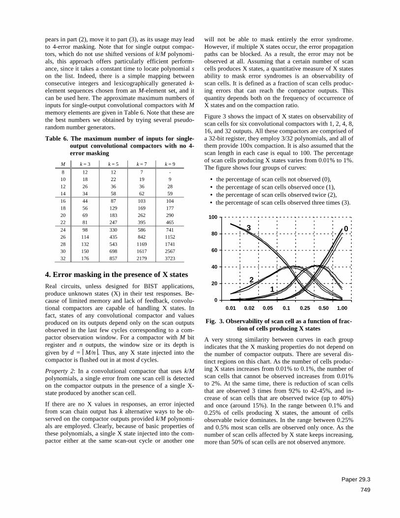
Figure 3 shows the impact of X states on observability of scan cells for six convolutional compactors with 1, 2, 4, 8, 16, and 32 outputs. All these compactors are comprised of a 32-bit register, they employ 3/32 polynomials, and all of them provide 100x compaction. It is also assumed that the scan length in each case is equal to 100. The percentage of scan cells producing X states varies from 0.01% to 1%. The figure shows four groups of curves:

• the percentage of scan cells not observed (0), • the percentage of scan cells observed once (1), • the percentage of scan cells observed twice (2), • the percentage of scan cells observed three times (3).

0

20

40

60

80

100

0.01 0.02 0.05 0.1 0.25 0.50 1.00

Fig. 3. Observability of scan cell as a function of frac-tion of cells producing X states

A very strong similarity between curves in each group indicates that the X masking properties do not depend on the number of compactor outputs. There are several dis-tinct regions on this chart. As the number of cells produc-ing X states increases from 0.01% to 0.1%, the number of scan cells that cannot be observed increases from 0.01% to 2%. At the same time, there is reduction of scan cells that are observed 3 times from 92% to 42-45%, and in-crease of scan cells that are observed twice (up to 40%) and once (around 15%). In the range between 0.1% and 0.25% of cells producing X states, the amount of cells observable twice dominates. In the range between 0.25% and 0.5% most scan cells are observed only once. As the number of scan cells affected by X state keeps increasing, more than 50% of scan cells are not observed anymore.

1 2

3 0

Paper 29.3

749

0,01

0,1

1

10

100

0.01 0.02 0.05 0.1 0.25 0.50 1.00

Fig. 4. Blocked scan cells due to X states

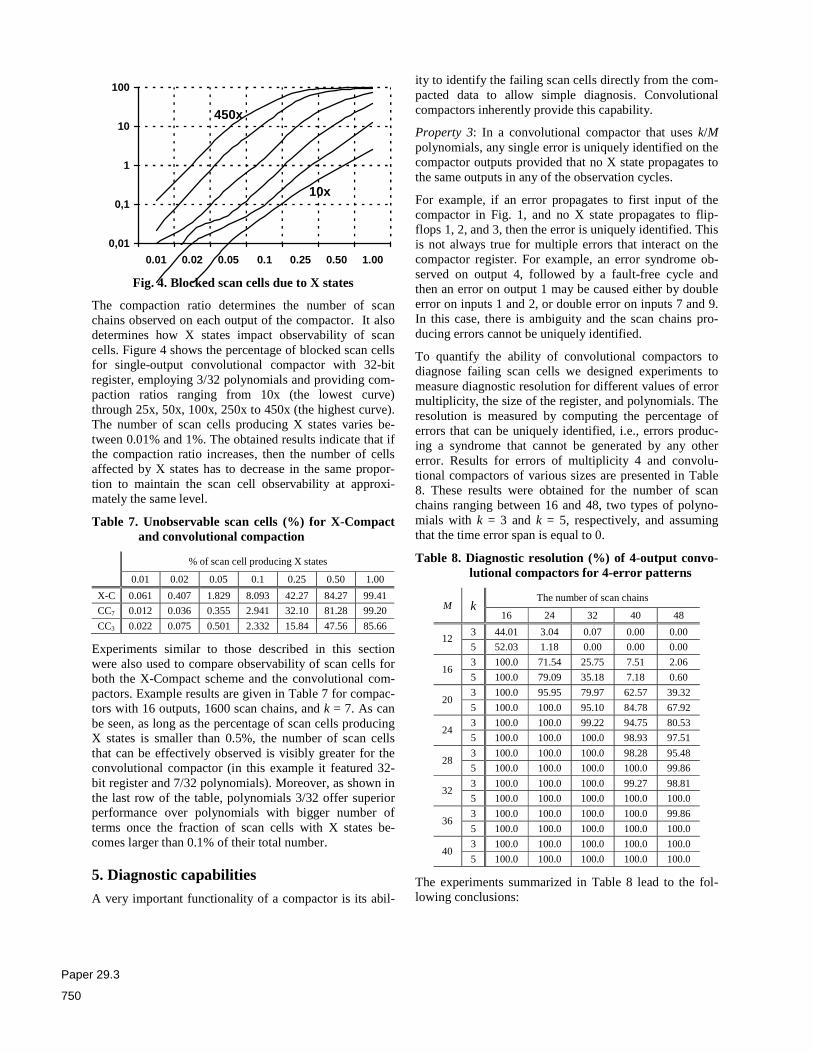
The compaction ratio determines the number of scan chains observed on each output of the compactor. It also determines how X states impact observability of scan cells. Figure 4 shows the percentage of blocked scan cells for single-output convolutional compactor with 32-bit register, employing 3/32 polynomials and providing com-paction ratios ranging from 10x (the lowest curve) through 25x, 50x, 100x, 250x to 450x (the highest curve). The number of scan cells producing X states varies be-tween 0.01% and 1%. The obtained results indicate that if the compaction ratio increases, then the number of cells affected by X states has to decrease in the same propor-tion to maintain the scan cell observability at approxi-mately the same level.

Table 7. Unobservable scan cells (%) for X-Compact and convolutional compaction

% of scan cell producing X states

0.01 0.02 0.05 0.1 0.25 0.50 1.00

X-C 0.061 0.407 1.829 8.093 42.27 84.27 99.41

CC7 0.012 0.036 0.355 2.941 32.10 81.28 99.20

CC3 0.022 0.075 0.501 2.332 15.84 47.56 85.66

Experiments similar to those described in this section were also used to compare observability of scan cells for both the X-Compact scheme and the convolutional com-pactors. Example results are given in Table 7 for compac-tors with 16 outputs, 1600 scan chains, and k = 7. As can be seen, as long as the percentage of scan cells producing X states is smaller than 0.5%, the number of scan cells that can be effectively observed is visibly greater for the convolutional compactor (in this example it featured 32-bit register and 7/32 polynomials). Moreover, as shown in the last row of the table, polynomials 3/32 offer superior performance over polynomials with bigger number of terms once the fraction of scan cells with X states be-comes larger than 0.1% of their total number.

5. Diagnostic capabilities

A very important functionality of a compactor is its abil-

ity to identify the failing scan cells directly from the com-pacted data to allow simple diagnosis. Convolutional compactors inherently provide this capability.

Property 3: In a convolutional compactor that uses k/M polynomials, any single error is uniquely identified on the compactor outputs provided that no X state propagates to the same outputs in any of the observation cycles.

For example, if an error propagates to first input of the compactor in Fig. 1, and no X state propagates to flip-flops 1, 2, and 3, then the error is uniquely identified. This is not always true for multiple errors that interact on the compactor register. For example, an error syndrome ob-served on output 4, followed by a fault-free cycle and then an error on output 1 may be caused either by double error on inputs 1 and 2, or double error on inputs 7 and 9. In this case, there is ambiguity and the scan chains pro-ducing errors cannot be uniquely identified.

To quantify the ability of convolutional compactors to diagnose failing scan cells we designed experiments to measure diagnostic resolution for different values of error multiplicity, the size of the register, and polynomials. The resolution is measured by computing the percentage of errors that can be uniquely identified, i.e., errors produc-ing a syndrome that cannot be generated by any other error. Results for errors of multiplicity 4 and convolu-tional compactors of various sizes are presented in Table 8. These results were obtained for the number of scan chains ranging between 16 and 48, two types of polyno-mials with k = 3 and k = 5, respectively, and assuming that the time error span is equal to 0.

Table 8. Diagnostic resolution (%) of 4-output convo-lutional compactors for 4-error patterns

The number of scan chains M k

16 24 32 40 48

3 44.01 3.04 0.07 0.00 0.00 12

5 52.03 1.18 0.00 0.00 0.00

3 100.0 71.54 25.75 7.51 2.06 16

5 100.0 79.09 35.18 7.18 0.60

3 100.0 95.95 79.97 62.57 39.32 20

5 100.0 100.0 95.10 84.78 67.92

3 100.0 100.0 99.22 94.75 80.53 24

5 100.0 100.0 100.0 98.93 97.51

3 100.0 100.0 100.0 98.28 95.48 28

5 100.0 100.0 100.0 100.0 99.86

3 100.0 100.0 100.0 99.27 98.81 32

5 100.0 100.0 100.0 100.0 100.0

3 100.0 100.0 100.0 100.0 99.86 36

5 100.0 100.0 100.0 100.0 100.0

3 100.0 100.0 100.0 100.0 100.0 40

5 100.0 100.0 100.0 100.0 100.0

The experiments summarized in Table 8 lead to the fol-lowing conclusions:

450x

10x

Paper 29.3

750

• increasing size of the compactor register improves diagnostic resolution,

• polynomials with higher number of terms (5) perform significantly better than polynomials with smaller number of terms (3) except for very small compac-tors and relatively large number of scans,

• diagnostic resolution decreases with the increasing compaction ratio.

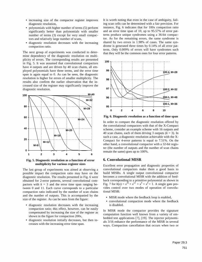
The next group of experiments was conducted to deter-mine dependency of the diagnostic resolution on multi-plicity of errors. The corresponding results are presented in Fig. 5. It was assumed that convolutional compactors have 4 outputs and are driven by 40 scan chains, all em-ployed polynomials have three terms, and the error time span is again equal to 0. As can be seen, the diagnostic resolution is higher for errors of smaller multiplicity. The results also confirm the earlier observation that the in-creased size of the register may significantly improve the diagnostic resolution.

Fig. 5. Diagnostic resolution as a function of error multiplicity for various register sizes

The last group of experiments was aimed at observing a possible impact the compaction ratio may have on the diagnostic resolution. The results presented in Fig. 6 were obtained for 2-error patterns, several convolutional com-pactors with k = 3 and the error time span ranging be-tween 0 and 11. Each curve corresponds to a particular compaction ratio indicated by the number of scan chains and the number of outputs. This is accompanied by the size of the register. As can be seen from the figure:

• diagnostic resolution decreases with the increasing compaction ratio; this effect, however, can be easily compensated by increasing the size of the register as shown in the figure for compaction 200x,

• diagnostic resolution initially decreases, but then in-creases with the increasing error time span.

It is worth noting that even in the case of ambiguity, fail-ing scan cells can be determined with a fair precision. For instance, Fig. 6 indicates that for 100x compaction ratio and an error time span of 10, up to 95.57% of error pat-terns produce unique syndromes using a 36-bit compac-tor. As for the remaining errors, the same syndrome is shared by two errors in 1.98% of cases. The same syn-drome is generated three times by 0.14% of all error pat-terns. Only 0.009% of errors will have syndromes such that they will be the common ones for four error patterns.

Fig. 6. Diagnostic resolution as a function of time span

In order to compare the diagnostic resolution offered by the convolutional compactors with that of the X-Compact scheme, consider an example scheme with 16 outputs and 40 scan chains, each of them driving 3 outputs (k = 3). In such a case, a diagnostic resolution achievable with the X-Compact for 4-error patterns is equal to 7.51%. On the other hand, a convolutional compactor with a 32-bit regis-ter (the number of outputs and the number of scan chains remain the same) goes up to 100%.

6. Convolutional MISR

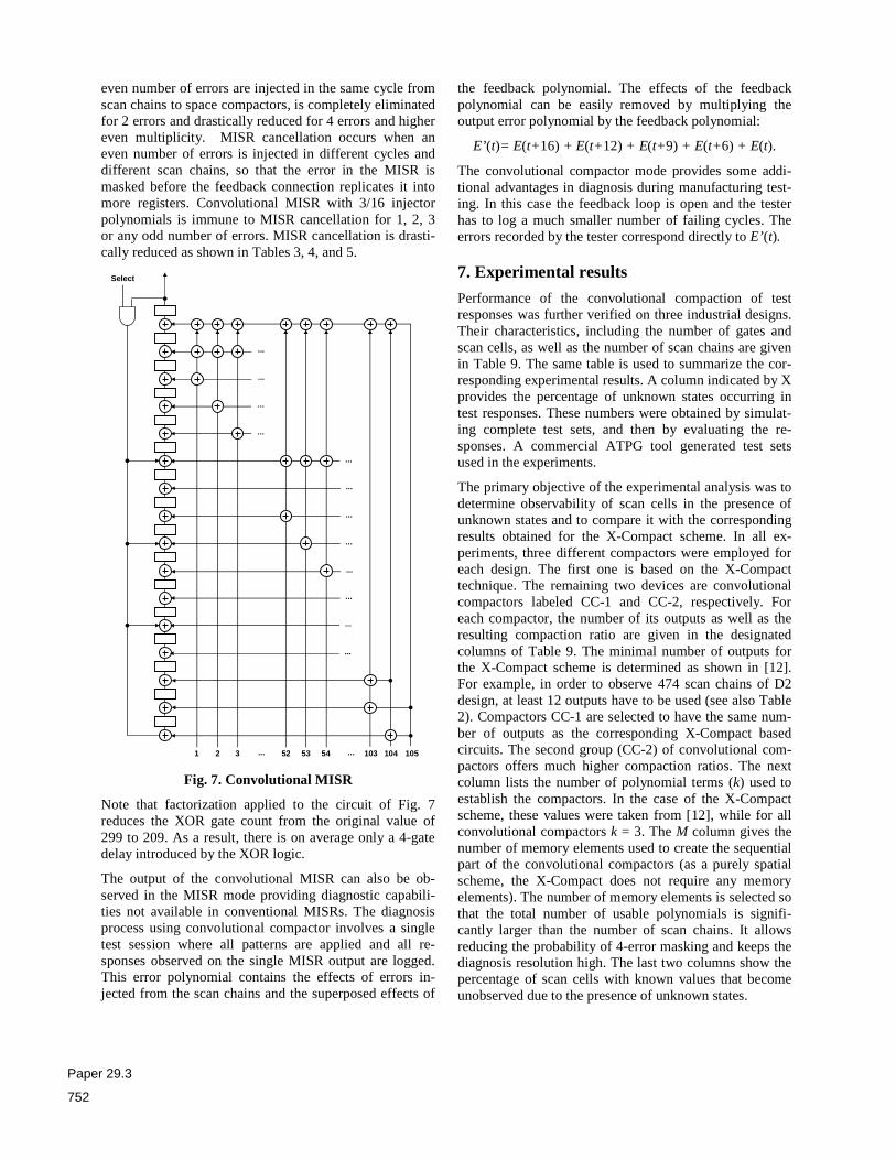
Excellent error propagation and diagnostic properties of convolutional compactors make them a good basis to build MISRs. A single output convolutional compactor becomes a convolutional MISR with the addition of feed-back corresponding to a primitive polynomial as shown in Fig. 7 for h(x) = x16 + x12 + x9 + x6 + 1. A single gate pro-vides control over two modes of operation of convolu-tional MISR:

• MISR mode where the feedback loop is enabled, • convolutional compaction mode where the feedback

is disabled.

In MISR mode the compactor provides the signature computation function well known from a variety of em-bedded test applications [7], [19]. The injector polynomi-als 3/16 enhance the performance of the MISR in several ways. Compaction cancellation that occurs when two or

95

96

97

98

99

100

0 2 4 6 8 10

100:1, M=36

100:4, M=28

200:1, M=48

100:2, M=32

0

20

40

60

80

100

1 2 3 4 5 6

M=8 M=12

M=16

M=20

M=24

M=28

M=32

M=40

Paper 29.3

751

even number of errors are injected in the same cycle from scan chains to space compactors, is completely eliminated for 2 errors and drastically reduced for 4 errors and higher even multiplicity. MISR cancellation occurs when an even number of errors is injected in different cycles and different scan chains, so that the error in the MISR is masked before the feedback connection replicates it into more registers. Convolutional MISR with 3/16 injector polynomials is immune to MISR cancellation for 1, 2, 3 or any odd number of errors. MISR cancellation is drasti-cally reduced as shown in Tables 3, 4, and 5.

Fig. 7. Convolutional MISR

Note that factorization applied to the circuit of Fig. 7 reduces the XOR gate count from the original value of 299 to 209. As a result, there is on average only a 4-gate delay introduced by the XOR logic.

The output of the convolutional MISR can also be ob-served in the MISR mode providing diagnostic capabili-ties not available in conventional MISRs. The diagnosis process using convolutional compactor involves a single test session where all patterns are applied and all re-sponses observed on the single MISR output are logged. This error polynomial contains the effects of errors in-jected from the scan chains and the superposed effects of

the feedback polynomial. The effects of the feedback polynomial can be easily removed by multiplying the output error polynomial by the feedback polynomial:

E’(t)= E(t+16) + E(t+12) + E(t+9) + E(t+6) + E(t).

The convolutional compactor mode provides some addi-tional advantages in diagnosis during manufacturing test-ing. In this case the feedback loop is open and the tester has to log a much smaller number of failing cycles. The errors recorded by the tester correspond directly to E’(t).

7. Experimental results

Performance of the convolutional compaction of test responses was further verified on three industrial designs. Their characteristics, including the number of gates and scan cells, as well as the number of scan chains are given in Table 9. The same table is used to summarize the cor-responding experimental results. A column indicated by X provides the percentage of unknown states occurring in test responses. These numbers were obtained by simulat-ing complete test sets, and then by evaluating the re-sponses. A commercial ATPG tool generated test sets used in the experiments.

The primary objective of the experimental analysis was to determine observability of scan cells in the presence of unknown states and to compare it with the corresponding results obtained for the X-Compact scheme. In all ex-periments, three different compactors were employed for each design. The first one is based on the X-Compact technique. The remaining two devices are convolutional compactors labeled CC-1 and CC-2, respectively. For each compactor, the number of its outputs as well as the resulting compaction ratio are given in the designated columns of Table 9. The minimal number of outputs for the X-Compact scheme is determined as shown in [12]. For example, in order to observe 474 scan chains of D2 design, at least 12 outputs have to be used (see also Table 2). Compactors CC-1 are selected to have the same num-ber of outputs as the corresponding X-Compact based circuits. The second group (CC-2) of convolutional com-pactors offers much higher compaction ratios. The next column lists the number of polynomial terms (k) used to establish the compactors. In the case of the X-Compact scheme, these values were taken from [12], while for all convolutional compactors k = 3. The M column gives the number of memory elements used to create the sequential part of the convolutional compactors (as a purely spatial scheme, the X-Compact does not require any memory elements). The number of memory elements is selected so that the total number of usable polynomials is signifi-cantly larger than the number of scan chains. It allows reducing the probability of 4-error masking and keeps the diagnosis resolution high. The last two columns show the percentage of scan cells with known values that become unobserved due to the presence of unknown states.

...

...

...

...

1 2 3 52 53 54 103 104 105

Select

... ...

...

...

...

...

...

...

...

...

Paper 29.3

752

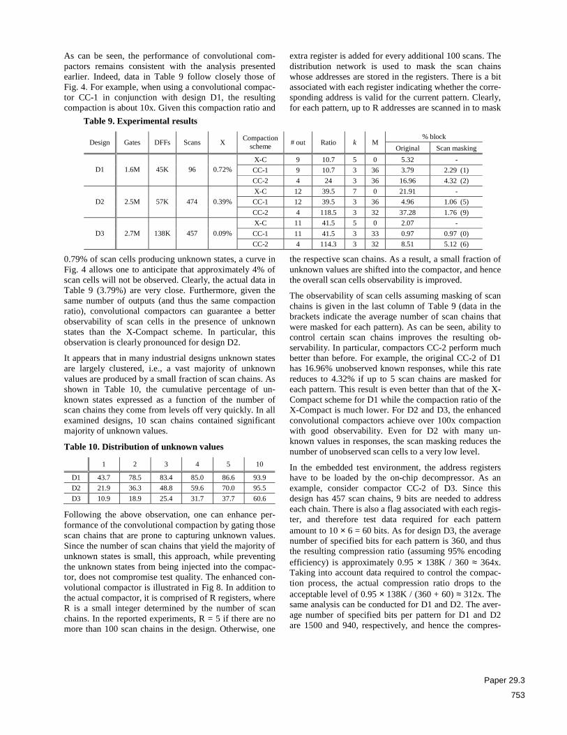
As can be seen, the performance of convolutional com-pactors remains consistent with the analysis presented earlier. Indeed, data in Table 9 follow closely those of Fig. 4. For example, when using a convolutional compac-tor CC-1 in conjunction with design D1, the resulting compaction is about 10x. Given this compaction ratio and

0.79% of scan cells producing unknown states, a curve in Fig. 4 allows one to anticipate that approximately 4% of scan cells will not be observed. Clearly, the actual data in Table 9 (3.79%) are very close. Furthermore, given the same number of outputs (and thus the same compaction ratio), convolutional compactors can guarantee a better observability of scan cells in the presence of unknown states than the X-Compact scheme. In particular, this observation is clearly pronounced for design D2.

It appears that in many industrial designs unknown states are largely clustered, i.e., a vast majority of unknown values are produced by a small fraction of scan chains. As shown in Table 10, the cumulative percentage of un-known states expressed as a function of the number of scan chains they come from levels off very quickly. In all examined designs, 10 scan chains contained significant majority of unknown values.

Table 10. Distribution of unknown values

1 2 3 4 5 10

D1 43.7 78.5 83.4 85.0 86.6 93.9

D2 21.9 36.3 48.8 59.6 70.0 95.5

D3 10.9 18.9 25.4 31.7 37.7 60.6

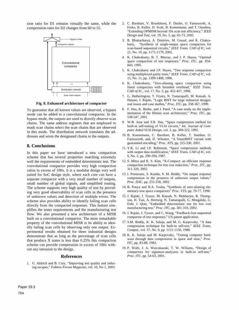
Following the above observation, one can enhance per-formance of the convolutional compaction by gating those scan chains that are prone to capturing unknown values. Since the number of scan chains that yield the majority of unknown states is small, this approach, while preventing the unknown states from being injected into the compac-tor, does not compromise test quality. The enhanced con-volutional compactor is illustrated in Fig 8. In addition to the actual compactor, it is comprised of R registers, where R is a small integer determined by the number of scan chains. In the reported experiments, R = 5 if there are no more than 100 scan chains in the design. Otherwise, one

extra register is added for every additional 100 scans. The distribution network is used to mask the scan chains whose addresses are stored in the registers. There is a bit associated with each register indicating whether the corre-sponding address is valid for the current pattern. Clearly, for each pattern, up to R addresses are scanned in to mask

the respective scan chains. As a result, a small fraction of unknown values are shifted into the compactor, and hence the overall scan cells observability is improved.

The observability of scan cells assuming masking of scan chains is given in the last column of Table 9 (data in the brackets indicate the average number of scan chains that were masked for each pattern). As can be seen, ability to control certain scan chains improves the resulting ob-servability. In particular, compactors CC-2 perform much better than before. For example, the original CC-2 of D1 has 16.96% unobserved known responses, while this rate reduces to 4.32% if up to 5 scan chains are masked for each pattern. This result is even better than that of the X-Compact scheme for D1 while the compaction ratio of the X-Compact is much lower. For D2 and D3, the enhanced convolutional compactors achieve over 100x compaction with good observability. Even for D2 with many un-known values in responses, the scan masking reduces the number of unobserved scan cells to a very low level.

In the embedded test environment, the address registers have to be loaded by the on-chip decompressor. As an example, consider compactor CC-2 of D3. Since this design has 457 scan chains, 9 bits are needed to address each chain. There is also a flag associated with each regis-ter, and therefore test data required for each pattern amount to 10 × 6 = 60 bits. As for design D3, the average number of specified bits for each pattern is 360, and thus the resulting compression ratio (assuming 95% encoding efficiency) is approximately 0.95 × 138K / 360 ≈ 364x. Taking into account data required to control the compac-tion process, the actual compression ratio drops to the acceptable level of 0.95 × 138K / (360 + 60) ≈ 312x. The same analysis can be conducted for D1 and D2. The aver-age number of specified bits per pattern for D1 and D2 are 1500 and 940, respectively, and hence the compres-

Table 9. Experimental results

% block Design Gates DFFs Scans X

Compaction scheme # out Ratio k M

Original Scan masking

X-C 9 10.7 5 0 5.32 -

CC-1 9 10.7 3 36 3.79 2.29 (1) D1 1.6M 45K 96 0.72%

CC-2 4 24 3 36 16.96 4.32 (2)

X-C 12 39.5 7 0 21.91 -

CC-1 12 39.5 3 36 4.96 1.06 (5) D2 2.5M 57K 474 0.39%

CC-2 4 118.5 3 32 37.28 1.76 (9)

X-C 11 41.5 5 0 2.07 -

CC-1 11 41.5 3 33 0.97 0.97 (0) D3 2.7M 138K 457 0.09%

CC-2 4 114.3 3 32 8.51 5.12 (6)

Paper 29.3

753

sion ratio for D1 remains virtually the same, while the compression ratio for D2 changes from 60 to 55.

Convolutionalcompactor

Scan chain outputs

Compactor outputs

…

Distribution network

Bypass mode

Fig. 8. Enhanced architecture of compactor

To guarantee that all known values are observed, a bypass mode can be added to a convolutional compactor. In the bypass mode, the outputs are used to directly observe scan chains. The same address registers that are employed to mask scan chains select the scan chains that are observed in this mode. The distribution network translates the ad-dresses and wires the designated chains to the outputs.

8. Conclusions

In this paper we have introduced a new compaction scheme that has several properties matching extremely well the requirements of embedded deterministic test. The convolutional compactor provides very high compaction ratios in excess of 100x. It is a modular design very well suited for SoC design style, where each core can have a separate compactor with a very small number of outputs, small number of global signals, and simplified routing. The scheme supports very high quality of test by provid-ing very good observability of scan cells in the presence of unknown values and detection of multiple errors. The scheme also provides ability to identify failing scan cells directly from the compacted responses. This feature sim-plifies the tester requirements and the manufacturing test flow. We also presented a new architecture of a MISR built on a convolutional compactor. The most remarkable property of the convolutional MISR is its ability to iden-tify failing scan cells by observing only one output. Ex-perimental results obtained for three industrial designs demonstrate that as long as the percentage of scan cells that produce X states is less than 0.25% this compaction scheme can provide compression in excess of 100x with-out any intrusion to the design.

References 1. G. Aldrich and B. Cory, “Improving test quality and reduc-

ing escapes,” Fabless Forum Magazine, vol. 10, No 1, 2003.

2. C. Barnhart, V. Brunkhorst, F. Distler, O. Farnsworth, A. Ferko, B. Keller, D. Scott, B. Koenemann, and T. Onodera, “Extending OPMISR beyond 10x scan test efficiency,” IEEE Design and Test, vol. 19, No. 5, pp. 65-73, 2002.

3. B. Bhattacharya, A. Dmitriev, M. Gossel, and K. Chakra-barty, “Synthesis of single-output space compactors for scan-based sequential circuits,” IEEE Trans. CAD of IC, vol. 21, No. 10, pp. 1171-1179, 2002.

4. K. Chakrabarty, B. T. Murray, and J. P. Hayes, “Optimal space compaction of test responses,” Proc. ITC, pp. 834-843, 1995.

5. K. Chakrabarty and J.P. Hayes, “Test response compaction using multiplexed parity trees,” IEEE Trans. CAD of IC, vol. 15, No. 11, pp. 1399-1408, 1996.

6. K. Chakrabarty, “Zero-aliasing space compaction using linear compactors with bounded overhead,” IEEE Trans. CAD of IC., vol. 17, No. 5, pp. 452-457, 1998.

7. G. Hetherington, T. Fryars, N. Tamarapalli, M. Kassab, A. Hassan, J. Rajski, “Logic BIST for large industrial designs: real issues and case studies,” Proc. ITC, pp. 358-367, 1999.

8. F. Hsu, K. Butler, and J. Patel, “A case study on the imple-mentation of the Illinois scan architecture,” Proc. ITC, pp. 538-547, 2001.

9. W-B. Jone and S.R. Das, “Space compression method for built-in self-testing of VLSI circuits,” Int. Journal of Com-puter Aided VLSI Design, vol. 3, pp. 309-322, 1991.

10. B. Koenemann, C. Barnhart, B. Keller, T. Snethen, O. Farnsworth, and, D. Wheater, “A SmartBIST variant with guaranteed encoding,” Proc. ATS, pp. 325-330, 2001.

11. Y.K. Li and J.P. Robinson, “Space compression methods with output data modification,” IEEE Trans. CAD of IC, vol. 6, No. 2, pp. 290-294, 1987.

12. S. Mitra and K. S. Kim, “X-Compact: an efficient response compaction technique for test cost reduction,” Proc. ITC, pp. 311-320, 2002.

13. I. Pomeranz, S. Kundu, S. M. Reddy, “On output response compression in the presence of unknown output values,” Proc. DAC, pp. 255-258, 2002.

14. B. Pouya and N.A. Touba, “Synthesis of zero-aliasing ele-mentary-tree space compactors” Proc. VTS, pp. 70-77, 1998.

15. J. Rajski, J. Tyszer, M. Kassab, N. Mukherjee, R. Thomp-son, H. Tsai, A. Hertwig, N. Tamarapalli, G. Mrugalski, G. Eide, J. Qian, “Embedded deterministic test for low cost manufacturing test,” Proc. ITC, pp. 301-310, 2002.

16. J. Rajski, J. Tyszer, and C. Wang, “Feedback-free sequential compactor of test responses,” US patent application.

17. S.M. Reddy, K. K. Saluja, and M. G. Karpovsky, “A data compression technique for built-in self-test,” IEEE Trans. Comput., vol. 37, No. 9, pp. 1151-1156, 1988.

18. K. K. Saluja and M. Karpovsky, “Testing computer hard-ware through data compression in space and time,” Proc. ITC, pp. 83-88, 1983.

19. P. Wohl, J. A. Waicukauski, T. W. Wiliams, “Design of compactors for signature-analyzers in built-in self-test,” Proc. ITC, pp. 54-63, 2001.

Paper 29.3

754