University of the Philippines Manila

College of Arts and Sciences

Department of Physical Sciences and Mathematics

RaDSS V02: A Radiolarian Classifier Using

Convolutional Neural Network

A special problem in partial fulfillment

of the requirements for the degree of

Bachelor of Science in Computer Science

Submitted by:

Micah P. Quisote

May 2018

Permission is given for the following people to have access to this SP:

Available to the general public Yes

Available only after consultation with author/SP adviser No

Available only to those bound by confidentiality agreement No

ACCEPTANCE SHEET

The Special Problem entitled “RaDSS V02: A Radiolarian Classifier Us-ing Convolutional Neural Network” prepared and submitted by Micah P. Quisote inpartial fulfillment of the requirements for the degree of Bachelor of Science in Com-puter Science has been examined and is recommended for acceptance.

Geoffrey A. Solano, Ph.D. (cand.)Adviser

EXAMINERS:Approved Disapproved

1. Gregorio B. Baes, Ph.D. (cand.)2. Avegail D. Carpio, M.Sc.3. Richard Bryann L. Chua, Ph.D. (cand.)4. Perlita E. Gasmen, M.Sc. (cand.)5. Marvin John C. Ignacio, M.Sc. (cand.)6. Vincent Peter C. Magboo, M.D., M.Sc.7. Ma. Sheila A. Magboo, M.Sc.

Accepted and approved as partial fulfillment of the requirements for the degreeof Bachelor of Science in Computer Science.

Ma. Sheila A. Magboo, M.Sc. Marcelina B. Lirazan, Ph.D.Unit Head Chair

Mathematical and Computing Sciences Unit Department of Physical SciencesDepartment of Physical Sciences and Mathematics

and Mathematics

Leonardo R. Estacio Jr., Ph.D.Dean

College of Arts and Sciences

i

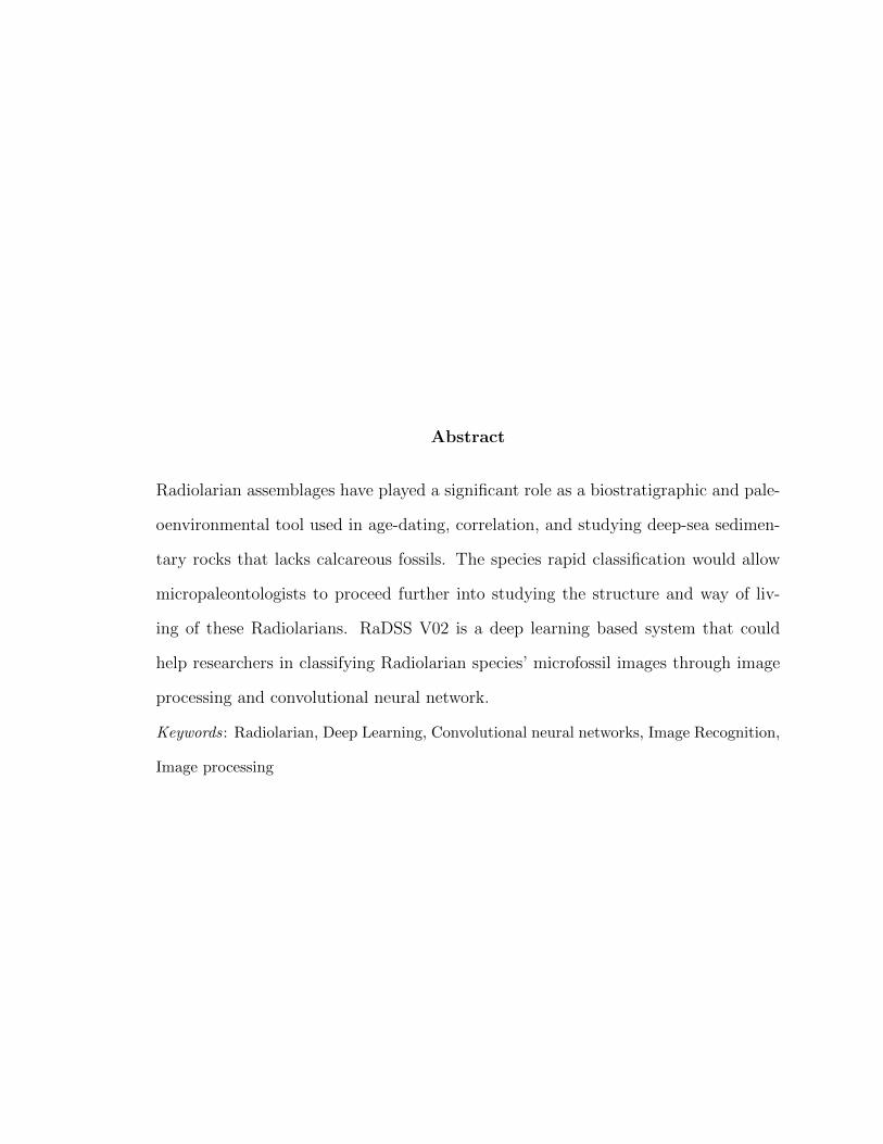
Abstract

Radiolarian assemblages have played a significant role as a biostratigraphic and pale-

oenvironmental tool used in age-dating, correlation, and studying deep-sea sedimen-

tary rocks that lacks calcareous fossils. The species rapid classification would allow

micropaleontologists to proceed further into studying the structure and way of liv-

ing of these Radiolarians. RaDSS V02 is a deep learning based system that could

help researchers in classifying Radiolarian species’ microfossil images through image

processing and convolutional neural network.

Keywords: Radiolarian, Deep Learning, Convolutional neural networks, Image Recognition,

Image processing

Contents

Acceptance Sheet i

Abstract ii

I. Introduction 1

A. Background of the Study . . . . . . . . . . . . . . . . . . . . . . . 1

B. Statement of the Problem . . . . . . . . . . . . . . . . . . . . . . . 3

C. Objectives of the Study . . . . . . . . . . . . . . . . . . . . . . . . 4

D. Significance of the Project . . . . . . . . . . . . . . . . . . . . . . 5

E. Scope and Limitations . . . . . . . . . . . . . . . . . . . . . . . . 6

F. Assumptions . . . . . . . . . . . . . . . . . . . . . . . . . . . . . . 6

II. Review of Related Literature 7

III. Theoretical Framework 12

A. Radiolarian . . . . . . . . . . . . . . . . . . . . . . . . . . . . . . 12

B. Machine Learning . . . . . . . . . . . . . . . . . . . . . . . . . . . 15

C. Deep Learning . . . . . . . . . . . . . . . . . . . . . . . . . . . . . 15

D. Convolutional Neural Network . . . . . . . . . . . . . . . . . . . . 16

D..1 Backpropagation . . . . . . . . . . . . . . . . . . . . . . . . . 19

IV. Design and Implementation 21

A. System Design . . . . . . . . . . . . . . . . . . . . . . . . . . . . . 21

A..1 RaDSS Training Module . . . . . . . . . . . . . . . . . . . . . 21

A..2 RaDSS Classifier App . . . . . . . . . . . . . . . . . . . . . . 26

B. System Architecture . . . . . . . . . . . . . . . . . . . . . . . . . . 29

C. Technical Architecture . . . . . . . . . . . . . . . . . . . . . . . . 30

V. Results 31

iii

A. RaDSS Training Module . . . . . . . . . . . . . . . . . . . . . . . 32

B. Classifier Application . . . . . . . . . . . . . . . . . . . . . . . . . 39

VI. Discussion 44

A. Dataset . . . . . . . . . . . . . . . . . . . . . . . . . . . . . . . . . 44

VII. Conclusion 46

VIII. Recommendation 47

IX. Bibliography 48

X. Appendix 51

A. Forms . . . . . . . . . . . . . . . . . . . . . . . . . . . . . . . . . 51

B. Source Code . . . . . . . . . . . . . . . . . . . . . . . . . . . . . . 51

XI. Acknowledgement 75

iv

I. Introduction

A. Background of the Study

Radiolarians have long been known for its beauty due to its numerous characteristics.

But other than its aesthetic structure, the organism is also very useful and can be

used as bio-stratigraphic and paleoenvironmental tool. They are zooplanktons that

drift around the oceans and sinks to the bottom of the ocean floor after their death.

Because of various reasons such as their existence over 500 million years ago, diver-

sity and abundance, their siliceous skeletons are important on the study of developing

history of the life on Earth based on their fossil records. [1]

However, despite of large body of research surrounding the Radiolaria species, the

classification of the said organism has proven to be very difficult. Existing traditional

methods of identifying radiolarians are based largely on the study of skeletons, ob-

servation and cross-referencing with known species. [2]

The use of technology in classifying Radiolaria has not yet given that much at-

tention by some specialists and the concerns of the taxonomical, morphological and

paleontological systematics mostly involve creation of information technologies like

databases rather than the pursuit of knowledge like classification, species discovery

and data creation.

Problems with automatic biological classifications has been explained by some

taxonomists, and Ebach et al. believes that we must first resolve certain matters like

issues on taxonomy of species before coming up with this kind of technology. Also,

there exists some misconception on the combination of technology and taxonomy with

the latter being threatened with slow-death. Bik, H.M. states that ”taxonomy should

1

be revamped and reborn for the modern age.” [3]

Therefore, time consuming conventional methods of biological classification that

involves the use of taxonomic keys, consulting reference books, catalogs, collecting,

observing, comparing species etc. must improve with automated classification that

could make the identification process more rapid to help the micropaleontologist’s

work done easier.

Machine learning has long been part of image processing and classification sys-

tems, and now have made its way through taxonomy. Some researchers focused on the

classification of plankton images and the The National Data Science Bowl 2015 com-

petition winner used Deep Neural Network in classifying greyscale images of plankton

into one of the 121 classes which achieved a 98% accuracy rate. [4] Research on zoo-

planktons have also been developed and Dai et al. created ZooplanktoNet, a deep

convolutional Network that classified zooplanktons which achieved an accuracy of

93.7%. [5]

Automatic classification system for the Radiolarian species have emerged for the

past years. Previous work of Apostol, et al. named RaDSS materialized the Radiolar-

ian classification using Support Vector Machine (SVM) and classified the Radiolarian

species into four classes. [6]. SVM is a type of the traditional machine learning where

manual feature extraction approach is used, most of the time through an external

feature extractor. Apostol et al. used ImageJ, a Java-based image processing and

analysis tool to do this. However, manual feature extraction involves algorithms that

detects only specific features and may leave behind other useful information that are

not covered by these algorithms.

2

Fimbres-Castro et al. used translation, rotation and scale invariant method to

identify the species. [7] Keceley et al. combined hand-crafted and deep features in

classifying the organism. [8]

With the advancement of deep learning and its consistent championship on the

ImageNet Large Scale Visual Recognition Competition (ILSVRC), the approach has

been a trigger behind numerous technologies and innovations. Deep learning is a

type of machine learning where manual feature extraction is replaced with layers of

algorithms to detect different features. Presently, there are different deep learning

architectures that are widely used in different applications, and some of them are

Alexnet and Caffenet. AlexNet is one of the pioneers in the ILSVRC to use deep

neural networks, while Caffenet is a variation of AlexNet that was created by Caffe

developers. Caffe is an open source deep learning framework which is written in C++,

with a Python interface. It is easier to understand, implement and switching between

CPU and GPU is simply set by a flag.

By using a deep convolutional neural network, RaDSS V02 will become one of

these technologies that aims to classify the Radiolarian species from an image. During

classification, the micropaleontologist may set a certain threshold value to determine

the minimum probability to achieve to classify the radiolarians microfossil image.

B. Statement of the Problem

Classification of the Radiolarian microfossil is normally done by traditional meth-

ods of ocular inspection and comparison with published images of radiolarians by

micropaleontologists, which is subjective in nature and time consuming. The first

version of RaDSS used machine learning employing manual feature extraction which

may not contain all the features, subjective since the user selects these from a list,

3

and may skip useful information.

C. Objectives of the Study

The purpose of this study is to develop a tool that automatically classifies micropho-

tographs of radiolarian species name. Specifically, it has the following objectives:

1. The main user is the micropaleontologist that can use the radiolarian classifier

model from the developed training module and can:

(a) Input a radiolarian microfossil image file or directory that contains these

images for classification item Apply preprocessing techniques to the radi-

olarian microfossil image

i. Resize and stretch the images

ii. Resize and pad around to maintain aspect ratio

(b) Set a threshold value that the classification should reach to assign the

image into a class. If the maximum probability is less than the threshold

value, classify the Radiolarian microfossil image as unknown.

(c) View the classification results and the probabilities obtained in the result

tab

(d) Download the result file containing the classification of the image, the

probabilities of the classificarion and details of the classifier model used

via a PDF

(e) View tutorial/help manual on how to use the radiolarian classifier

2. The AI Expert can use the training module with the following features:

(a) Input either of the following:

i. A microfossil image file of a radiolarian species and set its classification

4

ii. An directory containing the radiolarian species’ microfossil image and

an excel file that maps the filenames in this directory to Radiolarian

classes or labels

(b) Set the radiolarian species classification of the chosen microfossil image

(c) Apply preprocessing techniques to the radiolarian microfossil image

i. Resize and stretch the images

ii. Resize and pad around to maintain aspect ratio

(d) Choose which CNN architecture to train - whether Alexnet or Caffenet

(e) Input the CNN hyperparameters

i. Input the learning rate - the rate of the neural network on learning

ii. Input the number of iterations - the maximum number the images will

pass through the network

iii. Input the number of batch size - the number of images to train every

iteration

iv. Input the number of stepsize - the number of iteration to make to drop

the learning rate

(f) Build the CNN Model

i. Train and build the model using Caffe

ii. Cross validate model to get accuracy

D. Significance of the Project

Radiolarian assemblages can be very useful biostratigraphic and paleoenvironmental

tool in dating geological structures. Since classification is difficult in nature, using an

automated classifier will greatly help the micropaleontologist in deciding the species

class and will help improve this species taxonomy. Deep learning will be useful in

analyzing radiolarians complex structure and classify the species using this analysis.

5

E. Scope and Limitations

1. Species that can be classified by the tool is limited to classes that have at least

20 instances

2. The accuracy of the model is dependent on the number of data that are used

on training.

3. Only radiolarian microfossil jpeg images and corresponding excel label files are

accepted as input

4. The CNN architectures available for training and classification are fixed.

5. Learning rate, number of iterations, batch size, stepsize are fixed once trained

and being used already by the micropaleontologist.

6. Output file generated by the system is available in PDF format

F. Assumptions

1. The system is used by the researcher focusing on Radiolarian species

2. The system serves only as a guide to the researcher. The final classification of

the species will be identified by the micropaleontologist.

3. Input excel files for the training contain the labels of the species image. These

files are assumed to be correct and nonempty.

6

II. Review of Related Literature

Microfossils are perhaps the most important group of fossils because they are ex-

tremely useful in age-dating, correlation, paleoenvironmental reconstruction espe-

cially in the fields of oil industry, mining, engineering and billions of dollars have

been made based on microfossil studies. [9]

Vides, an expert system combining artificial intelligence and visual approach is

created by Swaby in identifying microfossils. It is in response to the problem of time

consuming identification of the microfossil on the deposits of the traditional manual

methods. Swaby implemented Lisp and IntelliCorps knowledge engineering environ-

ment (KEE) which helped the development of the user interface considerably. A

knowledge base builder created a code, data structure, graphical windows complete

with image and description to use as reference in identifying the input images. Clas-

sification is based on the presence or the absence of certain forms and structure of

the species. [10]

ONeill et al. created a system called GeoDAISY which is a modification of the

system DAISY (Digital Automated Identification System) to automatically identify

microfossils within a commercial stratigraphy environment. Some functionalities were

added like a caching mechanism based on Linux memory mapping, pattern correla-

tion and image rotation and scaling. It combined plastic self-organizing map neural

network technology and deep learning technique that was able to teach itself partially

and achieved 66.67% accuracy. [11]

Wong et al. used a dynamic hierarchical learning algorithm that implements both

supervised and unsupervised dynamic learning to accelerate microfossil identification.

Digital representations of the specimens are used to form clusters using Agglomerative

7

Hierarchical Clustering (AHC). Propagation and prioritization was then implemented

for the microfossil identification and achieved comparable rates to the best benchmark

results obtained using K-NN method. [12]

Deep learning algorithms have dominated the image recognition and classification

world. With its rapid development and wide popularity, researchers have implemented

the technique on various competitions and tasks to solve real world problems.

Tindall et al. used a convolutional neural network for plankton identification and

trained the data on a VGG16 architecture. Planktons are important to marine ecosys-

tem because of their role in the food web. Feeding data on a pre-trained architecture

is commonly known as transfer learning. The VGG16 is a 16-layer architecture that

consists of convolutional and max pooling layers is pre-trained using the ImageNet

dataset. In the paper, they fine-tuned the last layer to learn features of the plankton

dataset and achieved 85% accuracy. [13]

Jindal et al. also used CNN as a generic feature extractor with a random-forest

classifier on top of the hierarchy. It classified the plankton into 121 types presented

by Kaggle and Booz Allen Hamilton. They used various preprocessing and data

augmentation techniques before using the input images for training using minibatch

stochastic gradient descent with Nesterov momentum that achieved a logarithmic loss

of 0.75 which is on the top 10%. [14]

A CNN similar to the VGG architecture was used by Kuang. She implemented

the algorithm together with data augmentation, dropout regularization, leaky and

parametric ReLu activations and various model assembly methods to achieve classifi-

cation task. Among the different architectures, the 6 conv + 3 Fully connected layers

8

performs the best on the test set with 0.77 log loss. [15]

The National Data Science Bowl Competition winner also used CNN to classify

planktons and coded the program using Python with NumPy and Theano libraries.

They performed rescaling and global zero mean unit variance to pre-process the im-

ages then augmented the data based on various parameters like rotation, translation,

flipping, shearing and stretching. To avoid overfitting, implementation of judicious

techniques such as dropout, weight decay, data augmentation, pre-training, pseudo

labelling and parameter sharing was necessary. Their convnet architectures consist

of lots of conv layers with 3x3 filters and overlapping pooling with window size 3

and stride 2. Leaky ReLu was also implemented instead of only ReLu to introduce

nonlinearity to the data. One example of their architecture is composed of 13 layers

with parameters (10 conv and 3 fully connected) and 4 pooling layers. Trained using

stochastic gradient descent that took 24-28 hours, the best model achieved an accu-

racy of 82% on the validation set, and a top-5 accuracy of over 98%. [4]

Dai et al., inspired by the AlexNet and VGGNet architectures created Zooplank-

toNet, a deep convolutional network to classify zooplanktons automatically and ef-

fectively. It aims to capture more general and representative features than previous

predefined feature extraction algorithms. Their dataset consists of zooplankton im-

ages that involves 13 classes. Rescaling and subtracting the mean value over the

training set were done to pre-process the images and data augmentation techniques

like rotation, translation, shearing and flipping were also implemented. With a total

of 6 conv layers and 3 fully connected layers, the system achieved a 93.7% accuracy [5]

Foraminifera, a species that is also useful in age-dating, was classified using a

knowledge based system by Liu et al. To extract descriptive parameters from the

9

given set of images, they used computer vision techniques and the results were then

compared against a knowledge based system to infer its class. The knowledge based

system consists of descriptions to be used in a rule based classification approach. [16]

Pedraza et al. created an automated classification scheme for diatoms - microfos-

sils that are also studied as paleoenvironmental markers. They were classified into 80

types using a CNN model created after fine tuning a pre-trained AlexNet architec-

ture. It achieved a 99% accuracy. [17]

Some of the implementations of the papers above include various architectures

that have been developed by researchers in the deep learning community. The follow-

ing architectures won the ILSVRC competition starting from 2012, fueled the deep

learning movement and have been the foundation of computer scientists in building

their own deep model. One architecture that is very popular and the one that started

it all is the AlexNet architecture. This deep convolutional neural network needed to

classify the 1.2 million images from the ImageNet dataset into 1000 different classes.

The network is composed of 5 convolutional layers, some of which are followed by

max-pooling layers and dropout layers, and three fully connected layers. ReLu was

used to introduce nonlinearity to the data and data augmentation techniques that

consisted of image translations, horizontal reflections, and patch extractions. Trained

using batch stochastic gradient descent, the model achieved a 15.4% error rate, a first

on the ILSVRC competition. [18]

Zeiler and Fergus created ZFNet which is a fine tuning of the AlexNet. This ar-

chitecture achieved an 11.2% error rate and instead of using an 11x11 sized filters

in the first layer, they used a filter size of 7x7. The model used ReLUs for their

activation functions, cross-entropy loss for the error function, and was trained using

10

batch stochastic gradient descent.[19]

VGGNet, a 19-layered CNN architecture created by Karen Simonyan and Andrew

Zisserman introduced the use of 3x3 filters together with 2x2 max pooling layers.

They used ReLu layers after each convolutional layer and trained the model with

batch gradient descent. VGGNet achieved a 7.3% error rate. [20]

Szegedy et al. introduced the use of Inception modules in its architecture GoogleNet

in which some layers perform in parallel rather than the traditional sequential struc-

ture. This 22-layered architecture did not use fully connected layers but used average

pool instead and achieved a 6.7% error rate. [21]

Microsoft created its own neural network named ResNet which is a very deep,

152-layered architecture that achieved a 3.6% error rate. They introduced residual

blocks, wherein the input is fed on a conv-relu-conv series to obtain a residual map-

ping which is easier to optimize than the original mapping. This architecture brought

about the birth of very deep models and won the 2015 ILSVRC competition. [22]

The previous version of RaDSS that was created by Apostol et al. used Support

Vector Machine and principal component analysis to classify the radiolarian species.

It is written in Java and extracted the features of the input images using ImageJ

and JFeatureLib libraries. It was divided into 2 major functionalities, the training

module and the classifier app. The former is to be used by the training administrator

who will input some SVM parameters to train the model while the latter will take an

input to be classified into 4 classes of the species. [6]

11

III. Theoretical Framework

A. Radiolarian

Radiolarians are planktonic protists that are among the few groups with comprehen-

sive fossil records available for study. Formally, they belong to the Phyllum Protista,

Subphylum Sarcodina, Class Actinopoda, Subclass Radiolaria. [23] They are charac-

terized by their geometric and symmetric structure and live mainly in surface waters

with the earliest forms existed during the Cambrian age. Most are somewhat spheri-

cal, but a wide variety of shapes exist including cone-like and tetrahedral structures

that ranges anywhere from 30 microns to 2 mm in diameter. [2]

Figure 1. The radiolarian species

This unusual and often strikingly beautiful characteristic of these organisms is

their primary morphological characteristic, providing both a basis for their classifica-

tion and an insight into their ecology. [2]

Radiolarians transition corresponds to three transitions in the geologic time scale

namely the Permo-Triassic, Cretaceous-Tertiary and Paleogene-Neogene. They are

12

used in age-dating and the biostratigraphic correlation of oceanic sediments, partic-

ularly where calcareous microfossils have been dissolved. [2]

They have been studied extensively by paleontologists because of their well-established

presence in the fossil record and unique structure. The current methods for classifi-

cation are based largely on the study of skeletons from the orders Spumellaria and

Nassellaria using features of both the preservable skeleton and the soft parts.

The classification of Radiolaria recognizes two major groups: 1) the Polycystines,

with solid skeletal elements of simple opaline silica, and 2) the Phaeodarians, with

hollow skeletal elements of a complex siliceous composition that results in rapid dis-

solution in sea water and consequent rare preservation in sediments.

Polycystines structure and Phaeodarians structure

The Phaeodarians also possess a unique anatomical feature, a mass of tiny pig-

mented particles called the phaeodium. The polycystines, which are the radiolari-

ans best known to geologists, are subdivided into two major groups: the basically

spherical-shelled Spumellaria, and the basically conical-shelled Nassellaria. A few

polycystine groups lack a skeleton altogether. Some major groups of extinct radiolar-

ians differ substantially from both Spumellaria and Nassellaria, and may be ranked

13

at the same taxonomic level as those groups.

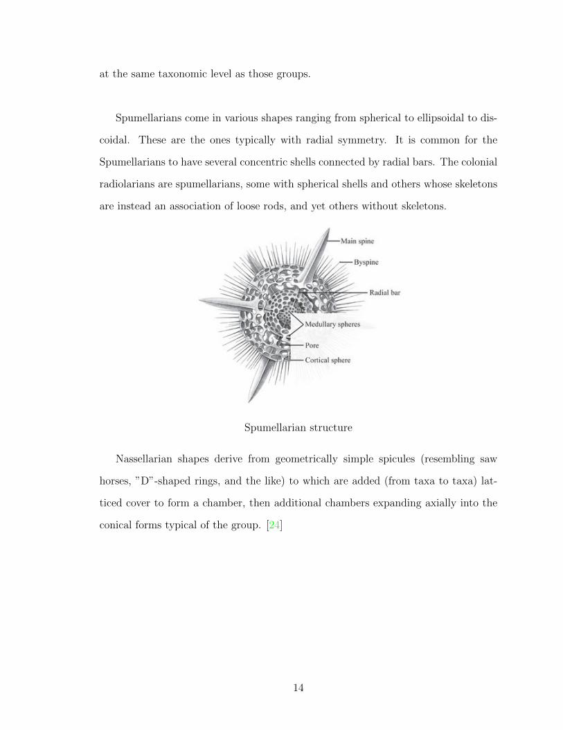
Spumellarians come in various shapes ranging from spherical to ellipsoidal to dis-

coidal. These are the ones typically with radial symmetry. It is common for the

Spumellarians to have several concentric shells connected by radial bars. The colonial

radiolarians are spumellarians, some with spherical shells and others whose skeletons

are instead an association of loose rods, and yet others without skeletons.

Spumellarian structure

Nassellarian shapes derive from geometrically simple spicules (resembling saw

horses, ”D”-shaped rings, and the like) to which are added (from taxa to taxa) lat-

ticed cover to form a chamber, then additional chambers expanding axially into the

conical forms typical of the group. [24]

14

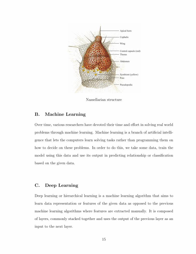
Nassellarian structure

B. Machine Learning

Over time, various researchers have devoted their time and effort in solving real world

problems through machine learning. Machine learning is a branch of artificial intelli-

gence that lets the computers learn solving tasks rather than programming them on

how to decide on these problems. In order to do this, we take some data, train the

model using this data and use its output in predicting relationship or classification

based on the given data.

C. Deep Learning

Deep learning or hierarchical learning is a machine learning algorithm that aims to

learn data representation or features of the given data as opposed to the previous

machine learning algorithms where features are extracted manually. It is composed

of layers, commonly stacked together and uses the output of the previous layer as an

input to the next layer.

15

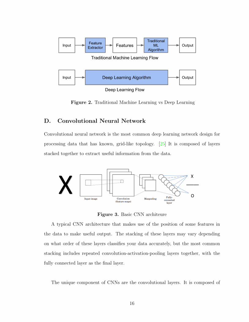
Figure 2. Traditional Machine Learning vs Deep Learning

D. Convolutional Neural Network

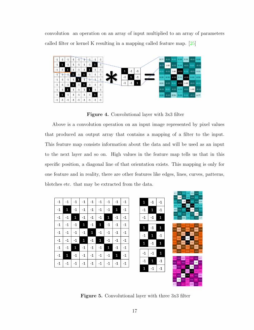
Convolutional neural network is the most common deep learning network design for

processing data that has known, grid-like topology. [25] It is composed of layers

stacked together to extract useful information from the data.

Figure 3. Basic CNN architeure

A typical CNN architecture that makes use of the position of some features in

the data to make useful output. The stacking of these layers may vary depending

on what order of these layers classifies your data accurately, but the most common

stacking includes repeated convolution-activation-pooling layers together, with the

fully connected layer as the final layer.

The unique component of CNNs are the convolutional layers. It is composed of

16

convolution an operation on an array of input multiplied to an array of parameters

called filter or kernel K resulting in a mapping called feature map. [25]

Figure 4. Convolutional layer with 3x3 filter

Above is a convolution operation on an input image represented by pixel values

that produced an output array that contains a mapping of a filter to the input.

This feature map consists information about the data and will be used as an input

to the next layer and so on. High values in the feature map tells us that in this

specific position, a diagonal line of that orientation exists. This mapping is only for

one feature and in reality, there are other features like edges, lines, curves, patterns,

blotches etc. that may be extracted from the data.

Figure 5. Convolutional layer with three 3x3 filter

17

The figure above shows three features, two diagonals with different orientation

and one x-like feature. All of these are stacked together to form a convolutional layer.

After the convolutional layer, an activation function is used to introduce nonlinearity

to the data.

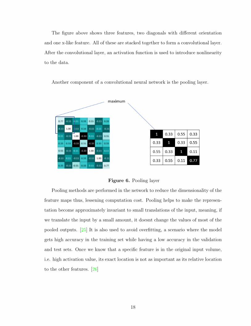
Another component of a convolutional neural network is the pooling layer.

Figure 6. Pooling layer

Pooling methods are performed in the network to reduce the dimensionality of the

feature maps thus, lessening computation cost. Pooling helps to make the represen-

tation become approximately invariant to small translations of the input, meaning, if

we translate the input by a small amount, it doesnt change the values of most of the

pooled outputs. [25] It is also used to avoid overfitting, a scenario where the model

gets high accuracy in the training set while having a low accuracy in the validation

and test sets. Once we know that a specific feature is in the original input volume,

i.e. high activation value, its exact location is not as important as its relative location

to the other features. [26]

18

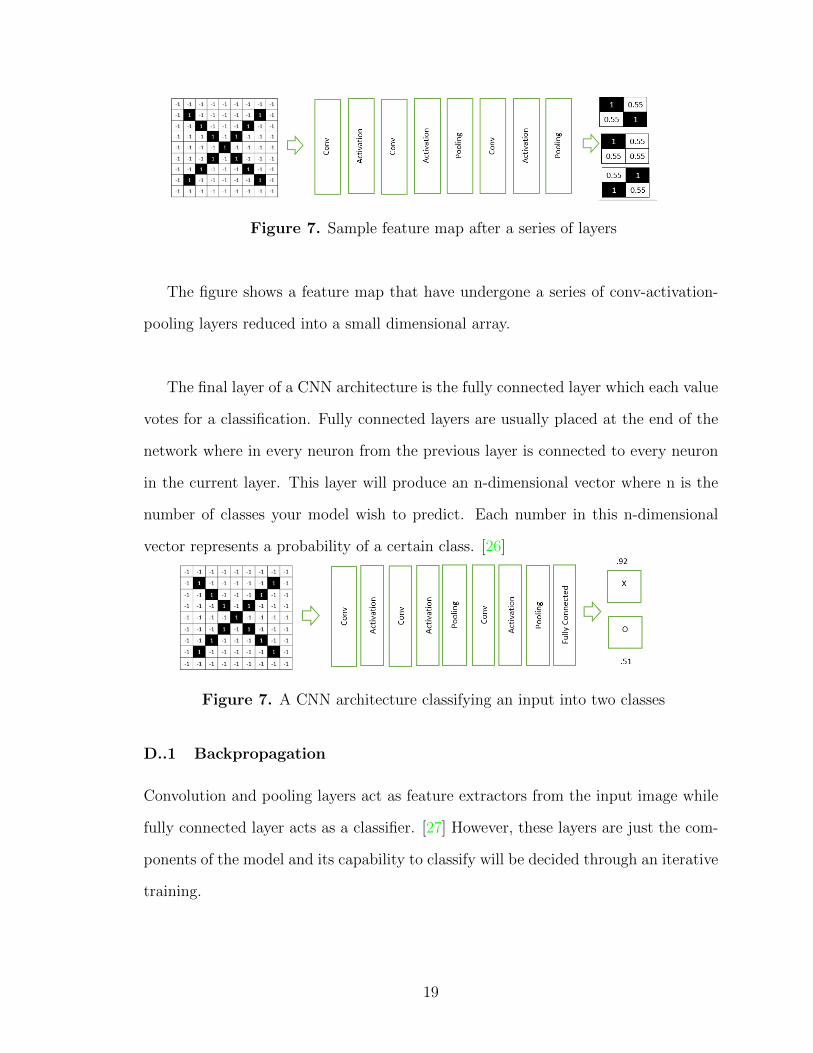
Figure 7. Sample feature map after a series of layers

The figure shows a feature map that have undergone a series of conv-activation-

pooling layers reduced into a small dimensional array.

The final layer of a CNN architecture is the fully connected layer which each value

votes for a classification. Fully connected layers are usually placed at the end of the

network where in every neuron from the previous layer is connected to every neuron

in the current layer. This layer will produce an n-dimensional vector where n is the

number of classes your model wish to predict. Each number in this n-dimensional

vector represents a probability of a certain class. [26]

Figure 7. A CNN architecture classifying an input into two classes

D..1 Backpropagation

Convolution and pooling layers act as feature extractors from the input image while

fully connected layer acts as a classifier. [27] However, these layers are just the com-

ponents of the model and its capability to classify will be decided through an iterative

training.

19

Basically, we train our model using the backpropagation algorithm forward pass,

loss function, backward pass, and weight update. [27] During the forward pass, the

input is fed into the network and outputs a classification. At first iteration, the model

will probably classify the image wrongly and the error could be computed using a

loss function.

We wanted to have low loss for our model to perform accurately, and to do this, we

wanted to know which parameters/weights contributed to that loss through backward

pass. We compute the gradient a multi-variable generalization of the derivative, of

the error with respect to all weights in the network. After knowing the gradient, we

update weights and parameters to minimize the output error.

The process of forward pass, loss function, backward pass, and parameter update

is just one training iteration. This process will be repeated for a fixed number of

iterations for each set of training images called a batch. Once you finish the parameter

update on the last training example, the network should be trained well enough so that

the weights of the layers are tuned correctly to create a high classification accuracy.

Hyperparameters like the number of iterations, number of epochs, batch size and

learning rate will be set before the training process.

20

IV. Design and Implementation

A. System Design

The system will be implemented using Python. It takes microfossil images of the

radiolarian species as input then apply little preprocessing techniques to normalize

the data. The pre-processed data is then be fed into the CNN model which will

extract the features itself and determine the species classification. The convolutional

neural network outputs the predicted species name. The generated outputs can be

downloaded at the end by the user in PDF format.

It is divided into 2 major functionalities: the training module and the classifier app.

The former builds the Radiolarian classifier model with the specified hyperparameters

while the classification of the radiolarian species is done by the classifier app.

A..1 RaDSS Training Module

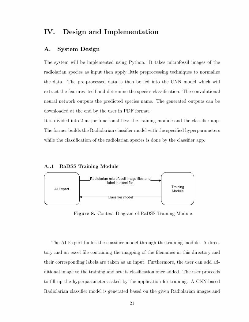
Figure 8. Context Diagram of RaDSS Training Module

The AI Expert builds the classifier model through the training module. A direc-

tory and an excel file containing the mapping of the filenames in this directory and

their corresponding labels are taken as an input. Furthermore, the user can add ad-

ditional image to the training and set its clasification once added. The user proceeds

to fill up the hyperparameters asked by the application for training. A CNN-based

Radiolarian classifier model is generated based on the given Radiolarian images and

21

specified hyperparameters through training. He is given an option to export this

classifier model to the classifier application.

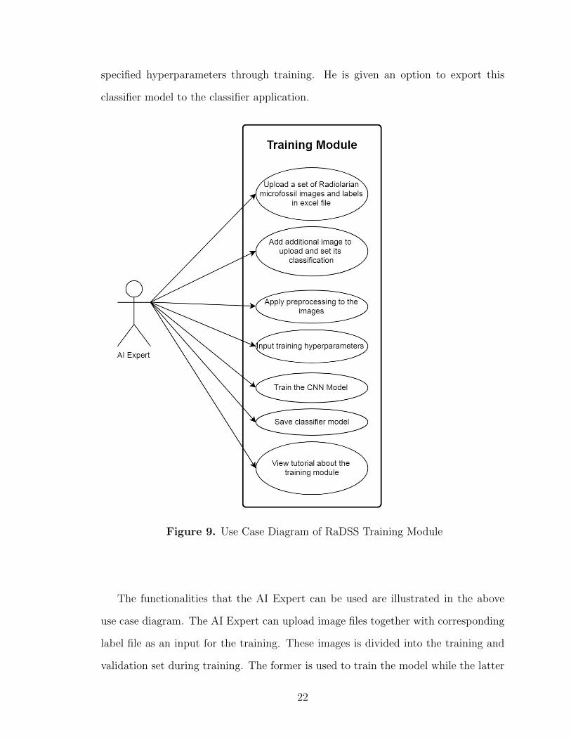
Figure 9. Use Case Diagram of RaDSS Training Module

The functionalities that the AI Expert can be used are illustrated in the above

use case diagram. The AI Expert can upload image files together with corresponding

label file as an input for the training. These images is divided into the training and

validation set during training. The former is used to train the model while the latter

22

is used to test the model to obtain accuracy. The user can also edit the classification

of the images, input training hyperparameters to train the model including the archi-

tecture to use, and finally save the model generated.

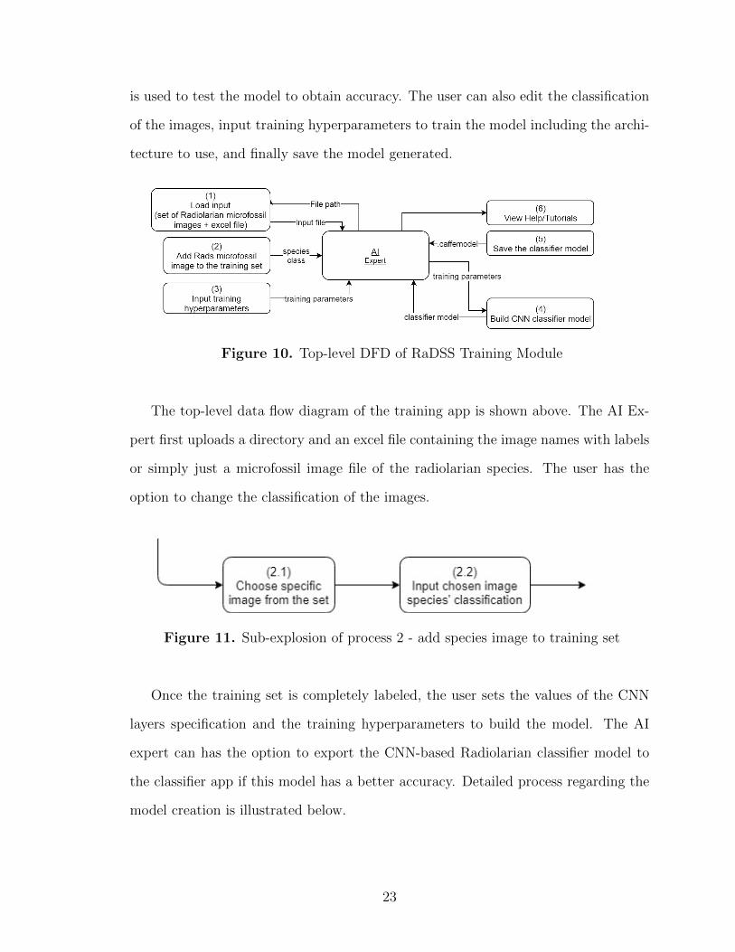
Figure 10. Top-level DFD of RaDSS Training Module

The top-level data flow diagram of the training app is shown above. The AI Ex-

pert first uploads a directory and an excel file containing the image names with labels

or simply just a microfossil image file of the radiolarian species. The user has the

option to change the classification of the images.

Figure 11. Sub-explosion of process 2 - add species image to training set

Once the training set is completely labeled, the user sets the values of the CNN

layers specification and the training hyperparameters to build the model. The AI

expert can has the option to export the CNN-based Radiolarian classifier model to

the classifier app if this model has a better accuracy. Detailed process regarding the

model creation is illustrated below.

23

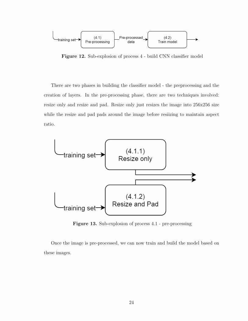
Figure 12. Sub-explosion of process 4 - build CNN classifier model

There are two phases in building the classifier model - the preprocessing and the

creation of layers. In the pre-processing phase, there are two techniques involved:

resize only and resize and pad. Resize only just resizes the image into 256x256 size

while the resize and pad pads around the image before resiizing to maintain aspect

ratio.

Figure 13. Sub-explosion of process 4.1 - pre-processing

Once the image is pre-processed, we can now train and build the model based on

these images.

24

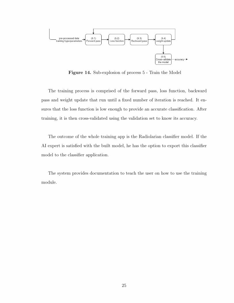
Figure 14. Sub-explosion of process 5 - Train the Model

The training process is comprised of the forward pass, loss function, backward

pass and weight update that run until a fixed number of iteration is reached. It en-

sures that the loss function is low enough to provide an accurate classification. After

training, it is then cross-validated using the validation set to know its accuracy.

The outcome of the whole training app is the Radiolarian classifier model. If the

AI expert is satisfied with the built model, he has the option to export this classifier

model to the classifier application.

The system provides documentation to teach the user on how to use the training

module.

25

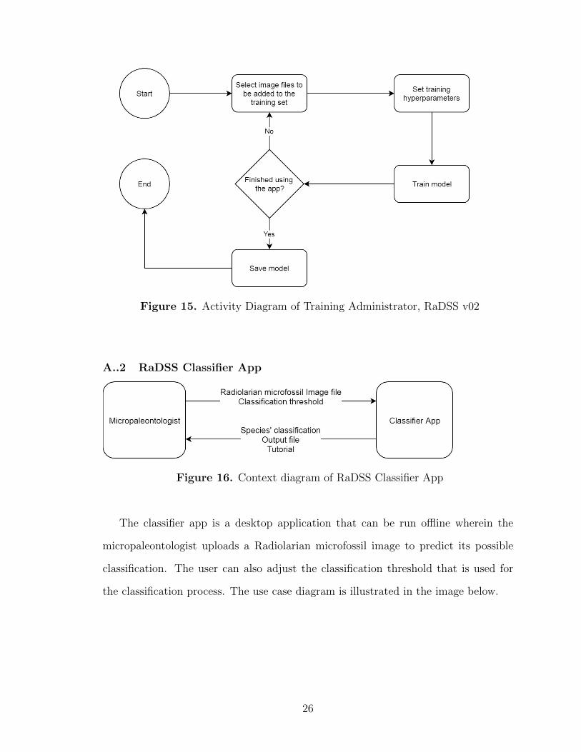
Figure 15. Activity Diagram of Training Administrator, RaDSS v02

A..2 RaDSS Classifier App

Figure 16. Context diagram of RaDSS Classifier App

The classifier app is a desktop application that can be run offline wherein the

micropaleontologist uploads a Radiolarian microfossil image to predict its possible

classification. The user can also adjust the classification threshold that is used for

the classification process. The use case diagram is illustrated in the image below.

26

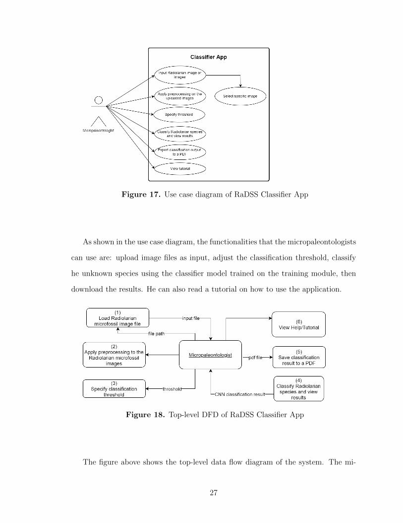
Figure 17. Use case diagram of RaDSS Classifier App

As shown in the use case diagram, the functionalities that the micropaleontologists

can use are: upload image files as input, adjust the classification threshold, classify

he unknown species using the classifier model trained on the training module, then

download the results. He can also read a tutorial on how to use the application.

Figure 18. Top-level DFD of RaDSS Classifier App

The figure above shows the top-level data flow diagram of the system. The mi-

27

cropaleontologist inputs an unknown Radiolarian microfossil image to be classified to

one of the classes provided by the system. The image is then pre-processed then fed

into the Radiolarian classifier model for classification. Further details can be seen in

the following diagram.

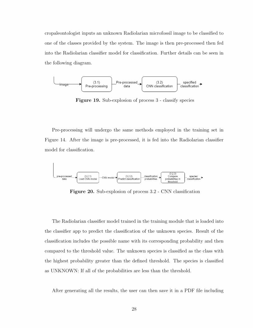
Figure 19. Sub-explosion of process 3 - classify species

Pre-processing will undergo the same methods employed in the training set in

Figure 14. After the image is pre-processed, it is fed into the Radiolarian classifier

model for classification.

Figure 20. Sub-explosion of process 3.2 - CNN classification

The Radiolarian classifier model trained in the training module that is loaded into

the classifier app to predict the classification of the unknown species. Result of the

classification includes the possible name with its corresponding probability and then

compared to the threshold value. The unknown species is classified as the class with

the highest probability greater than the defined threshold. The species is classified

as UNKNOWN: If all of the probabilities are less than the threshold.

After generating all the results, the user can then save it in a PDF file including

28

the image, the classification, the probability, and the details of the classifier model use.

An option to adjust the classification threshold is also available for the micropa-

leontologist and is used to determine the predicted class of the unknown species.

Finally, the user can view tutorials and read the documentation on how to use the

system. Screenshots and help instructions is provided together with the summary of

commands, panes and operations offered by the application.

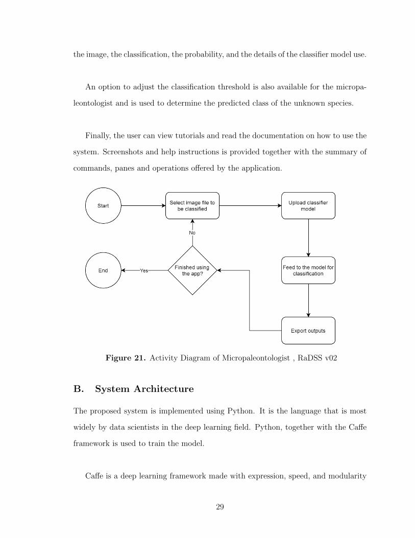
Figure 21. Activity Diagram of Micropaleontologist , RaDSS v02

B. System Architecture

The proposed system is implemented using Python. It is the language that is most

widely by data scientists in the deep learning field. Python, together with the Caffe

framework is used to train the model.

Caffe is a deep learning framework made with expression, speed, and modularity

29

in mind. It is developed by Berkeley AI Research (BAIR) and by community con-

tributors. It supports CNN and other deep learning network designs. The models are

defined by configuration without hard-coding and training can switch between CPU

and GPU by setting a single flag. [28]

C. Technical Architecture

1. Windows 7 or Higher;

2. 2 Ghz CPU

3. RAM: 8 GB or higher

4. Graphical Processing Unit (GPU), preferably NVIDIA

5. 2 Gigabytes disk space

30

V. Results

The Radiolarian Decision Support System v02 is a standalone desktop application

created using python. It is divided into two parts, the Training Module and the

Classifier Application that can be used by the AI expert and the microplaeontologist

respectively.

Figure 20. RaDSS v02 Main Window

31

A. RaDSS Training Module

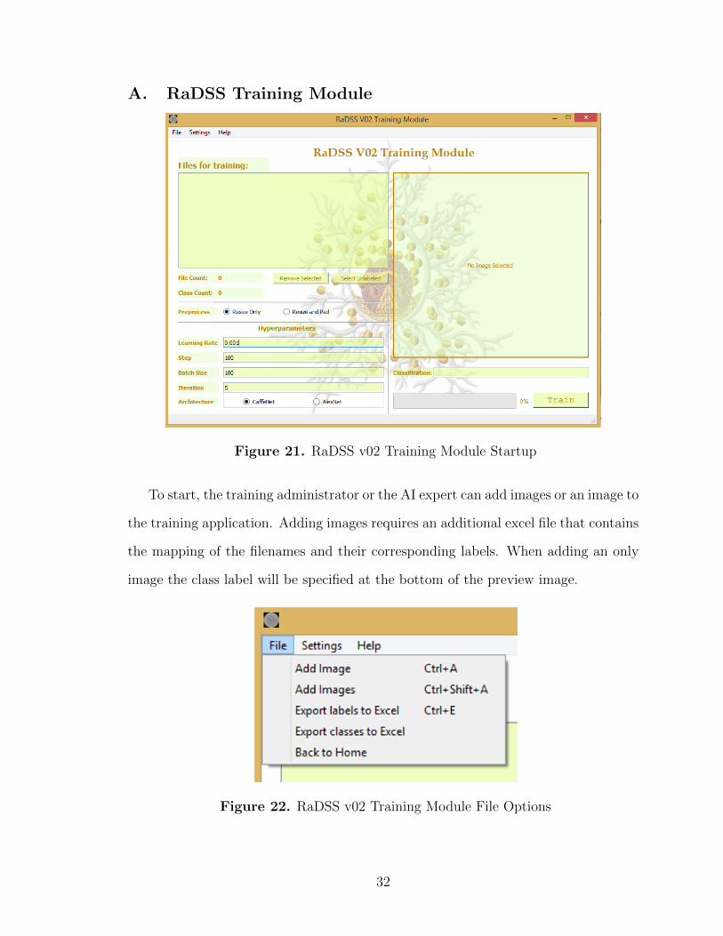
Figure 21. RaDSS v02 Training Module Startup

To start, the training administrator or the AI expert can add images or an image to

the training application. Adding images requires an additional excel file that contains

the mapping of the filenames and their corresponding labels. When adding an only

image the class label will be specified at the bottom of the preview image.

Figure 22. RaDSS v02 Training Module File Options

32

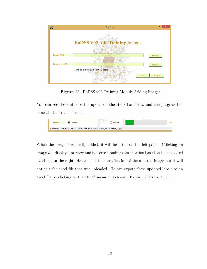
Figure 23. RaDSS v02 Training Module Adding Images

You can see the status of the upoad on the staus bar below and the progress bar

beneath the Train button.

When the images are finally added, it will be listed on the left panel. Cliicking an

image will display a preview and its corresponding classification based on the uploaded

excel file on the right. He can edit the classification of the selected image but it will

not edit the excel file that was uploaded. He can export these updated labels to an

excel file by clicking on the ”File” menu and choose ”Export labels to Excel.”

33

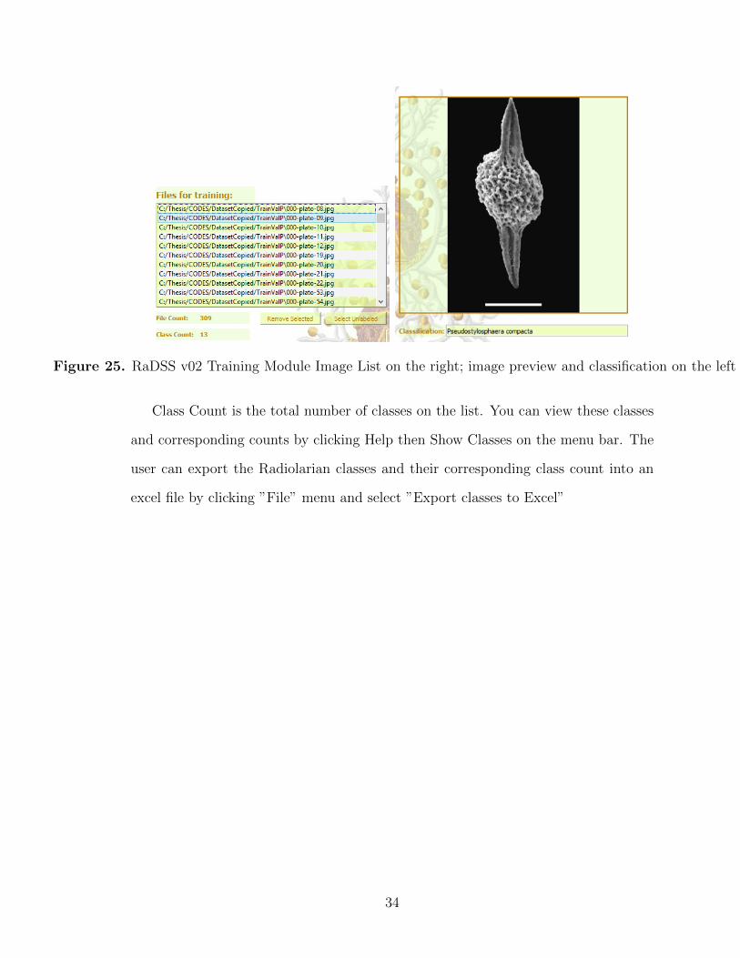
Figure 25. RaDSS v02 Training Module Image List on the right; image preview and classification on the left

Class Count is the total number of classes on the list. You can view these classes

and corresponding counts by clicking Help then Show Classes on the menu bar. The

user can export the Radiolarian classes and their corresponding class count into an

excel file by clicking ”File” menu and select ”Export classes to Excel”

34

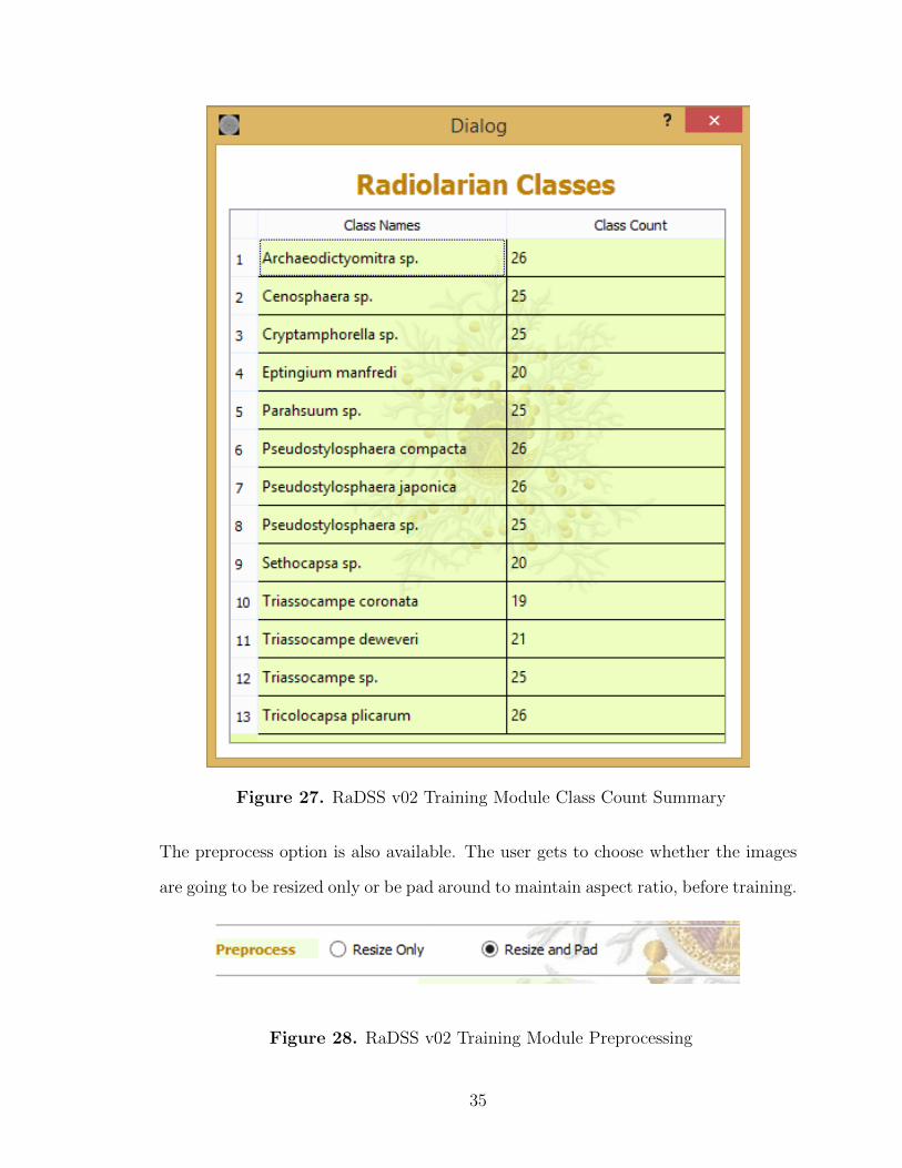
Figure 27. RaDSS v02 Training Module Class Count Summary

The preprocess option is also available. The user gets to choose whether the images

are going to be resized only or be pad around to maintain aspect ratio, before training.

Figure 28. RaDSS v02 Training Module Preprocessing

35

To train a Radiolarian classifier model, the training administrator will input the

hyperparameters.

Figure 29. RaDSS v02 Training Module Hyperparameters

The hyperparameters are the most important part of the module. These are the

specifications to be used during training. Learning Rate: The default is set to 0.001

and it should be small as possible. This will set how fast or slow the network will

learn. Too high learning rate may result to overfitting while too low value may result

to an underfit.

Step: Step or stepsize drops the learning rate every step iterations. Meaning, the

learning rate will drop on the specified step iteration.

Batch Size: Batch size is the number of images that will be used to train the network

per iteration. It is usually a divisible of the total number of training images.

Iteration: Iteration is the total number of passes the images to the network.

Models: Models are the currently available architectures or neural nets that will be

trained using the training images. These architectures have once been the state-of-

the-art on the image classification fields.

The training is displayed on an external command prompt that can be viewed

an monitor by the AI expert. The trained model will be saved on the models path

that can be edited in the configuration. It is saved in a .caffemodel format and

36

automatically be made available on the classifier application.

After training, the resulting plot and the training accuracy is displayed. This

accuracy is computed based on the model’s performance on the validation set. The

AI expert has the option to export this caffemodel to the classifier application if it

has better performance than that on the classifier application.

Figure 30. RaDSS v02 Training Module Plot of Training

More information about the different modules and how to use the application can

be found in the User’s Manual and can be viewed by clicking ”Help/Tutorials” under

”Help” menu.

37

Figure 31. RaDSS v02 Training Module Tutorials

The Radiolarian classifier models created in this module plays a significant role in

the classifier application. It will be used to predict the possible classification of the

unknown Radiolarian species.

38

B. Classifier Application

Figure 32. RaDSS v02 Classifier Application Startup

To start using the application, the micropaleontologist can either input a directory

of images or an image for classification. Only jpeg images are accepted by the system.

Figure 33. RaDSS v02 Classifier Application File Options

After choosing a directory, the image files will be loaded to the list on the left,

showing the file count on the upper right of the list. The user can also view the image

preview on the right tabbed pane. The 1st tab contains image, while the 2nd tab

provides the summary of the classification, i.e. the class name and the probabilities

39

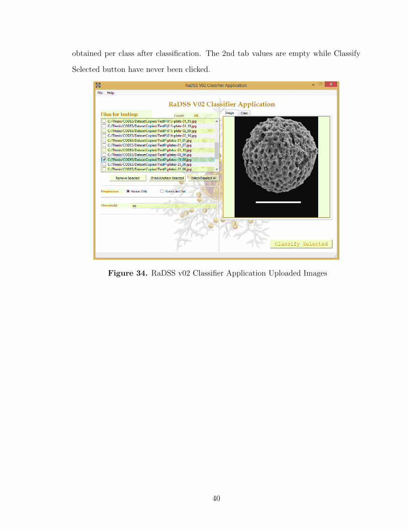
obtained per class after classification. The 2nd tab values are empty while Classify

Selected button have never been clicked.

Figure 34. RaDSS v02 Classifier Application Uploaded Images

40

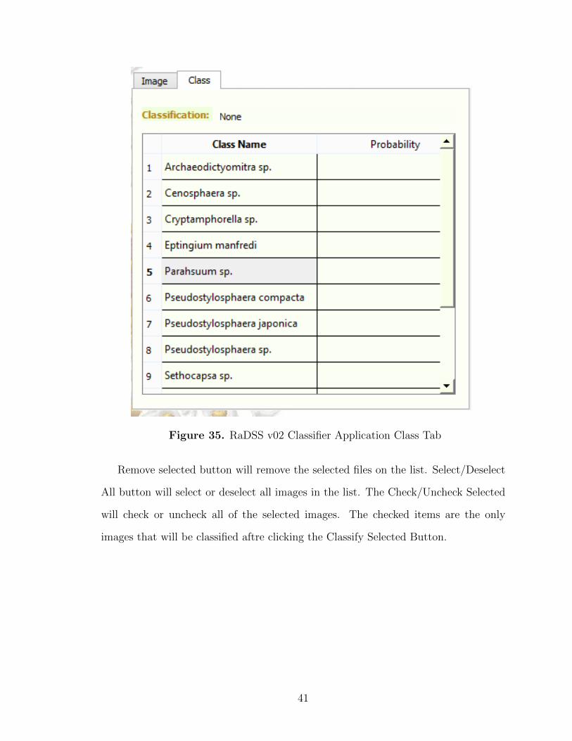
Figure 35. RaDSS v02 Classifier Application Class Tab

Remove selected button will remove the selected files on the list. Select/Deselect

All button will select or deselect all images in the list. The Check/Uncheck Selected

will check or uncheck all of the selected images. The checked items are the only

images that will be classified aftre clicking the Classify Selected Button.

41

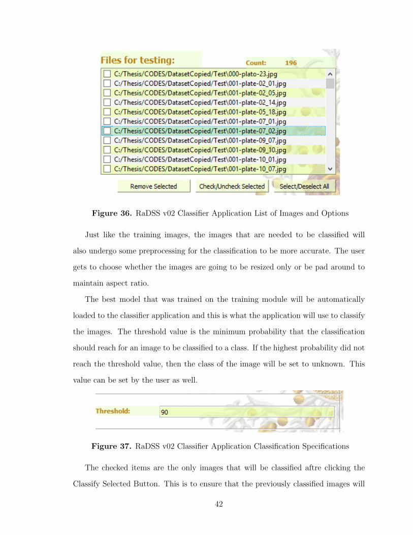
Figure 36. RaDSS v02 Classifier Application List of Images and Options

Just like the training images, the images that are needed to be classified will

also undergo some preprocessing for the classification to be more accurate. The user

gets to choose whether the images are going to be resized only or be pad around to

maintain aspect ratio.

The best model that was trained on the training module will be automatically

loaded to the classifier application and this is what the application will use to classify

the images. The threshold value is the minimum probability that the classification

should reach for an image to be classified to a class. If the highest probability did not

reach the threshold value, then the class of the image will be set to unknown. This

value can be set by the user as well.

Figure 37. RaDSS v02 Classifier Application Classification Specifications

The checked items are the only images that will be classified aftre clicking the

Classify Selected Button. This is to ensure that the previously classified images will

42

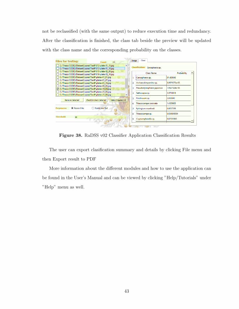
not be reclassified (with the same output) to reduce execution time and redundancy.

After the classification is finished, the class tab beside the preview will be updated

with the class name and the corresponding probability on the classes.

Figure 38. RaDSS v02 Classifier Application Classification Results

The user can export clasification summary and details by clicking File menu and

then Export result to PDF

More information about the different modules and how to use the application can

be found in the User’s Manual and can be viewed by clicking ”Help/Tutorials” under

”Help” menu as well.

43

VI. Discussion

A. Dataset

The dataset comprises a total of 3,820 microfossil images of various Radiolarian

species and were used to test the application. These images were provided by Pro-

fessor Edanjarlo Marquez which are in the form of digital and printed (which were

scanned).

Preprocessing The only preprocessing performed on the data is rescaling and can

be done using the python’s OpenCV library.

Classes Since the Radiolarian classes present on the dataset have unequal number

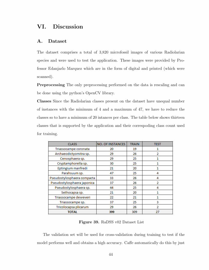
of instances with the minimum of 4 and a maximum of 47, we have to reduce the

classes so to have a minimum of 20 intances per class. The table below shows thirteen

classes that is supported by the application and their correspoding class count used

for training.

Figure 39. RaDSS v02 Dataset List

The validation set will be used for cross-validation during training to test if the

model performs well and obtains a high accuracy. Caffe automatically do this by just

44

specifying the validation set.

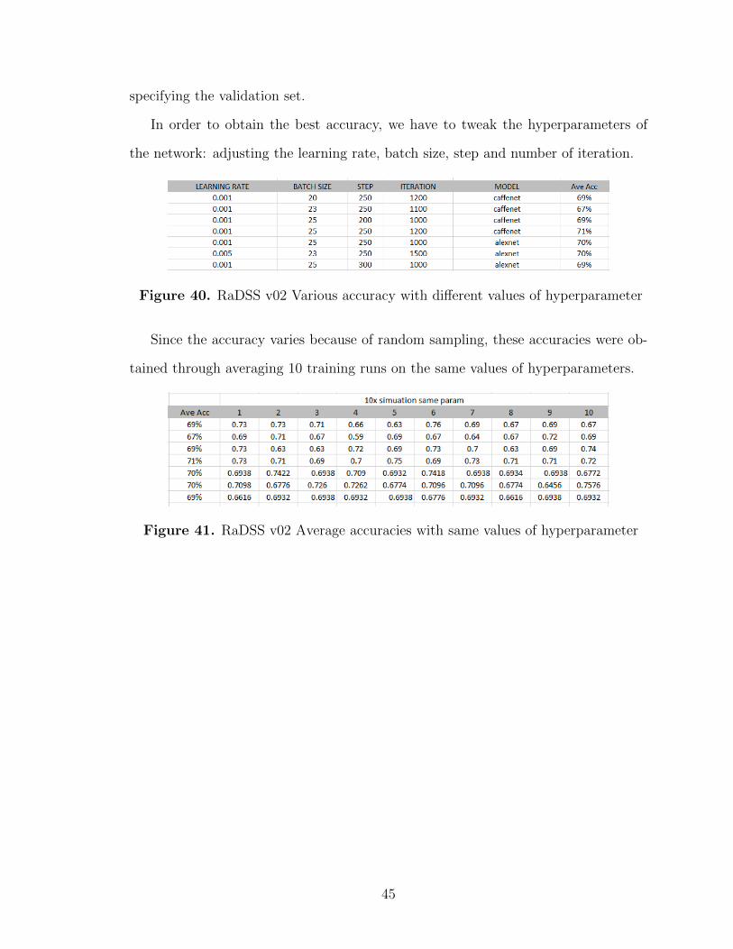
In order to obtain the best accuracy, we have to tweak the hyperparameters of

the network: adjusting the learning rate, batch size, step and number of iteration.

Figure 40. RaDSS v02 Various accuracy with different values of hyperparameter

Since the accuracy varies because of random sampling, these accuracies were ob-

tained through averaging 10 training runs on the same values of hyperparameters.

Figure 41. RaDSS v02 Average accuracies with same values of hyperparameter

45

VII. Conclusion

RaDSS v02 is an application that will help the micropaleontologist in classifying

Radiolarian species. It is made possible by Deep Learning algorithms, in this case,

the convolutional neural network. With miniman preprocessing, it is able to analize

raw Radiolarian microfossil image and tweaking the hyperparameters might improve

the accuracy. The result containing the information about the classification can be

exported through a PDF.

46

VIII. Recommendation

RaDSS v02’s accuracy will greatly increase if there are more data and instances per

class. The more data in a convolutional neural network, the more learning it will get.

Also, some heavy architectures like googleNet or ResNet might perform better

than the ones availbale in RaDSS v02. Augmentation will also help increase the

number of data and will ensure that the model performs well even with the different

orientation of an image.

47

IX. Bibliography

[1] “Radiolaria — new world encyclopedia,” New World Encyclopedia, 2015. n.p.

Web. 04 January 2018.

[2] M. Asaravala, H. Lam, S. Litty, J. Phillips, and T.-T. Wu, “Introduction to the

radiolaria,” 2000. n.p. Web. 04 January 2018.

[3] H. M. Bik, “Lets rise up to unite taxonomy and technology,” PLOS Biology,

vol. 15, pp. 1–4, 08 2017.

[4] A. van den Oord, I. Korshunova, J. Burms, J. Degrave, L. Pigou, P. Buteneers,

and S. Dieleman, “Classifying plankton with deep neural networks,” March 2015.

n.p. Web. 04 January 2018.

[5] J. Dai, R. Wang, H. Zheng, G. Ji, and X. Qiao, “Zooplanktonet: Deep convo-

lutional network for zooplankton classification,” in OCEANS 2016 - Shanghai,

pp. 1–6, April 2016.

[6] L. A. Apostol, E. Marquez, P. Gasmen, and G. Solano, “Radss: A radiolarian

classifier using support vector machines,” 2016 7th International Conference on

Information, Intelligence, Systems & Applications (IISA), pp. 1–6, 2016.

[7] C. Fimbres-Castro, J. Alvarez-Borrego, I. Vazquez-Martinez, T. L. Espinoza-

Carreon, A. E. Ulloa-Perez, and M. A. Bueno-Ibarra, “Nonlinear correlation by

using invariant identity vectors signatures to identify plankton,” Gayana (Con-

cepcion), vol. 77, pp. 105 – 124, 00 2013.

[8] A. S. Keceli, A. Kaya, and S. U. Keceli, “Classification of radiolarian images

with hand-crafted and deep features,” Computers and Geosciences, vol. 109,

pp. 67–74, Dec. 2017.

[9] J. H. Lipps, “Microfossils,” n.p. n.d. Web. 04 January 2018.

48

[10] P. A. Swaby, “Vides: an expert system for visually identifying microfossils,”

IEEE Expert, vol. 7, pp. 36–42, April 1992.

[11] M. A. O’Neill and M. Denos, “Automating biostratigraphy in oil and gas explo-

ration: Introducing geodaisy,” Journal of Petroleum Science and Engineering,

vol. 149, no. Supplement C, pp. 851 – 859, 2017.

[12] D. J. Cindy M. Wong, “Dynamic hierarchical algorithm for accelerated micro-

fossil identification,” Proceedings SPIE Image Processing: Machine Vision Ap-

plications VIII, vol. 9405, pp. 1 – 15, 2015.

[13] L. Tindall, C. Luong, and A. Saad, “Plankton classification using vgg16 net-

work,” 2015.

[14] P. Jindal and R. Mundra, “Plankton classification using hybrid convolutional

network-random forests architectures,”

[15] Y. Kuang, “Deep neural network for deep sea plankton classification,” 2015.

[16] S. Liu, M. Thonnat, and M. Berthod, “Automatic classification of planktonic

foraminifera by a knowledge-based system,” in Proceedings of the Tenth Confer-

ence on Artificial Intelligence for Applications, pp. 358–364, Mar 1994.

[17] A. Pedraza, G. Bueno, O. Deniz, G. Cristbal, S. Blanco, and M. Borrego-Ramos,

“Automated diatom classification (part b): A deep learning approach,” Applied

Sciences, vol. 7, no. 5, 2017.

[18] A. Krizhevsky, I. Sutskever, and G. E. Hinton, “Imagenet classification with

deep convolutional neural networks,” in Proceedings of the 25th International

Conference on Neural Information Processing Systems - Volume 1, NIPS’12,

(USA), pp. 1097–1105, Curran Associates Inc., 2012.

49

[19] M. D. Zeiler and R. Fergus, Visualizing and Understanding Convolutional Net-

works, pp. 818–833. Cham: Springer International Publishing, 2014.

[20] K. Simonyan and A. Zisserman, “Very deep convolutional networks for large-scale

image recognition,” CoRR, vol. abs/1409.1556, 2014.

[21] C. Szegedy, V. Vanhoucke, S. Ioffe, J. Shlens, and Z. Wojna, “Rethinking the

inception architecture for computer vision,” 2016 IEEE Conference on Computer

Vision and Pattern Recognition (CVPR), pp. 2818–2826, 2016.

[22] K. He, X. Zhang, S. Ren, and J. Sun, “Deep residual learning for image recog-

nition,” 2016 IEEE Conference on Computer Vision and Pattern Recognition

(CVPR), pp. 770–778, 2016.

[23] “Radiolaria,” Miracle, 2002. n.p. Web. 04 January 2018.

[24] “What are radiolarians,” n.p. n.d. Web. 04 January 2018.

[25] I. Goodfellow, Y. Bengio, and A. Courville, Deep Learning. MIT Press, 2016.

http://www.deeplearningbook.org.

[26] A. Deshpande, “A beginner’s guide to understanding convolutional neural net-

work,” n.p. n.d. Web. 04 January 2018.

[27] U. Karn, “An intuitive explanation of convolutional neural networks,” August

2016. n.p. Web. 04 January 2018.

[28] “Caffe,” n.p. n.d. Web. 04 January 2018.

50

X. Appendix

A. Forms

B. Source Code

import s e t t i n g simport sysimport osimport cv2import numpy as npimport globimport randomimport c a f f eimport timeimport subprocessimport datet imeimport p l o t l e a r n i n g c u r v e as p l cfrom PyQt5 . u i c import loadUifrom PyQt5 import QtGui , QtCorefrom r eadF i l e s import Fi leReaderfrom PyQt5 . QtCore import pyqtSlotfrom PyQt5 . QtWidgets import ∗from PyQt5 . QtGui import ∗from c o l l e c t i o n s import Counterfrom augmentor import augmentfrom PIL import Imagefrom create lmdb import CreateLMDBfrom func t oo l s import p a r t i a lfrom preproce s s import PreprocessImage as prfrom create html import createHTML

c l a s s MainApp(QMainWindow ) :de f i n i t ( s e l f ) :

super (MainApp , s e l f ) . i n i t ( )s e l f . show home ( )

de f show home ( s e l f ) :loadUi ( s e t t i n g s . u i path + ’mainApp . ui ’ , s e l f )s e l f . setWindowTitle (”RaDSS V02”)s e l f . setWindowIcon (QtGui . QIcon ( s e t t i n g s . i con path ) )

# −− code below connects ac t i on to the buttons /menu/ etcs e l f . t ra inBtn . c l i c k ed . connect ( s e l f . show tra in ing app )s e l f . c l a s sBtn . c l i c k ed . connect ( s e l f . show test app )

s e l f . actionLoad Manual . t r i g g e r ed . connect ( s e l f . loadManual )

de f c learLayout ( layout ) :whi le layout . count ( ) :

c h i l d = layout . takeAt (0)i f c h i l d . widget ( ) i s not None :

ch i l d . widget ( ) . d e l e t eLa t e r ( )e l i f c h i l d . layout ( ) i s not None :

c learLayout ( ch i l d . layout ( ) )de f show tra in ing app ( s e l f ) :

loadUi ( s e t t i n g s . u i path + ’ trainApp . ui ’ , s e l f )s e l f . setWindowTitle (”RaDSS V02 Training Module ”)s e l f . setWindowIcon (QtGui . QIcon ( s e t t i n g s . i con path ) )

# INSTANCE VARIABLESs e l f . label map = [ ]s e l f . c l a s s e s = [ ]s e l f . c lassCount = [ ]s e l f . a r c h i t e c t u r e = ” c a f f e n e t ”s e l f . currentItem = None

# −− code below connects ac t i on to the buttons /menu/ etcs e l f . t ra inButton . c l i c k ed . connect ( s e l f . t ra in data method )#s e l f . t ra inButton . c l i c k ed . connect ( s e l f . t ra in data temp )s e l f . removeButton . c l i c k ed . connect ( s e l f . r emove se l e c t ed )s e l f . s e lUn labe l ed . c l i c k ed . connect ( s e l f . s e l e c t a l l u n l a b e l e d )

#don ’ t remove menu ac t i on s ! f o r examples e l f . actionAdd Images . t r i g g e r ed . connect ( s e l f . add images )s e l f . actionAdd Image . t r i g g e r ed . connect ( s e l f . add image )s e l f . a c t i onEd i t Con f i gu ra t i on . t r i g g e r ed . connect ( s e l f . e d i t c o n f i g u r a t i o n )s e l f . a c t i onExpo r t l ab e l s . t r i g g e r ed . connect ( s e l f . e x p o r t l a b e l s )s e l f . actionBack to Home . t r i g g e r e d . connect ( s e l f . show home )

51

s e l f . a c t i onShow c la s s e s . t r i g g e r ed . connect ( s e l f . showClasses )s e l f . actionLoad Manual . t r i g g e r ed . connect ( s e l f . loadManual )

s e l f . l i s t t r a i n i n g im a g e s . i temCl icked . connect ( s e l f . image c l i cked prev i ew )s e l f . im a g e c l a s s i f i c a t i o n . re turnPres sed . connect ( s e l f . c l a s s i f i c a t i o n c h a n g e d )

# va l i d a t o r ss e l f . b a t ch s i z e . s e tVa l i da to r ( QIntVal idator ( ) )s e l f . i t e r n o . s e tVa l i da to r ( QIntVal idator ( ) )s e l f . t r a i n s t e p . s e tVa l i da to r ( QIntVal idator ( ) )

# se t i n i t i a l f i e l d ss e l f . f i l e c n t . setText (”0”)s e l f . c l s c n t . setText (”0”)

de f show test app ( s e l f ) :loadUi ( s e t t i n g s . u i path + ’ testApp . ui ’ , s e l f )s e l f . setWindowTitle (”RaDSS V02 C l a s s i f i e r Appl i cat ion ”)s e l f . setWindowIcon (QtGui . QIcon ( s e t t i n g s . i con path ) )

# Instance Var iab l e ss e l f . c l a s s e s = np . load ( s e t t i n g s . data path + ” c l a s sD i c t . npy”)s e l f . currentItem = Nones e l f . p r e d i c t i o n s = [ ]

# one dimens ional array that corresponds to the i n d i c e s o f l i s t t e s t i n g im a g e ss e l f . probab = [ ]s e l f . thresh = 90 .

# −− code below connects ac t i on to the buttons /menu/ etc

s e l f . c l a s s i f yBu t t on . c l i c k ed . connect ( s e l f . tes t data method )s e l f . s e l e c tA l lB tn . c l i c k ed . connect ( s e l f . s e l e c t a l l )s e l f . chkSelectedBtn . c l i c k ed . connect ( s e l f . c h e ck s e l e c t ed )s e l f . btnRemove . c l i c k ed . connect ( s e l f . t e s t r emove s e l e c t ed )

#don ’ t remove menu ac t i on s ! f o r examples e l f . act ionAdd Images Test . t r i g g e r ed . connect ( s e l f . t e s t add images )s e l f . actionAdd Image Test . t r i g g e r ed . connect ( s e l f . t e s t add image )s e l f . actionExport to PDF . t r i g g e r ed . connect ( s e l f . exportToPDF)s e l f . actionBack to Home . t r i g g e r e d . connect ( s e l f . show home )s e l f . actionLoad Manual . t r i g g e r ed . connect ( s e l f . loadManual )

s e l f . l i s t t e s t i n g im a g e s . i temCl icked . connect ( s e l f . t e s t imag e c l i c k ed p r e v i ew )s e l f . th r e sho ld . r e turnPres sed . connect ( s e l f . thresho ld changed )

# populate tab l e with the c l a s s e sf o r row , c l s in enumerate ( s e l f . c l a s s e s ) :

s e l f . tableWidget . insertRow ( row )s e l f . tableWidget . set I tem ( row , 0 , QTableWidgetItem ( c l s ) )

p r in t (”Model to use : ” , s e t t i n g s . c l a s s i f i e r m o d e l )

###################################################################################################################################################################################### TRAIN MODULE METHODS ####################################

# cr ea t e s an abso lu t e f i l ename−l a b e l array s e l f . t r a i n and s e l f . va l@pyqtSlot ( )de f t ra in data method ( s e l f ) :

p r i n t (” Train ”)

i f s e l f . v a l i d a t e i npu t s ( ) == False :re turn

s e l f . completed = 0

# de f au l t i s c a f f e n e t ; check i f a lexNet i s chosenni f s e l f . a lexNet . isChecked ( ) :

s e l f . a r c h i t e c t u r e = ” a l exnet ”

# save c l a s s d i c t i ona rys e l f . c o un t c l a s s e s ( )np . save ( s e t t i n g s . data path + ” c l a s sD i c t . npy” , s e l f . c l a s s e s )

# ed i t prototxt f i l e s based on hyperparameters s e t by users e l f . update prog re s s bar (” Creat ing s o l v e r pototxt s . . . ” , 1)s e l f . e d i t p r o t o t x t s ( )

# s h u f f l e the l i s t ( t h i s i s 2 d imens ional so use np)# checked and working#pr in t (∗ s e l f . label map , sep=’\n ’ )np . random . s h u f f l e ( s e l f . label map )

# working# d iv ide t r a i n and va l randomlys e l f . update prog re s s bar (” Div id ing t r a i n and va l s e t . . . ” , 2)s e l f . t r a i n = [ ]s e l f . va l = [ ]f o r i in range ( l en ( s e l f . label map ) ) :

temp = s e l f . label map [ i ] [ : ] # [ : ] i s nece s sa ry to pass by value ! !

52

temp [ 1 ] = s e l f . get image num labe l ( temp [ 1 ] )# put a l l that i s d i v i s i b l e by f i v e to the va l set , t h i s w i l l comprise 20% of the datai f ( i % 5 == 0 ) :

s e l f . va l . append ( temp)e l s e :

s e l f . t r a i n . append ( temp)# mappings# array : image [ 0 ] with l a b e l : l a b e l [ 0 ]s e l f . t r a i n da ta = [ ]s e l f . t r a i n l a b e l = [ ]s e l f . va l data = [ ]s e l f . v a l l a b e l = [ ]

s e l f . update prog re s s bar (” Converting Images to Array . . . ” , 2)

# Working ! : Convert and Augment# convert each TRAIN f i l enames to nparray and augmentf o r imahe in s e l f . t r a i n :

# −− opt i ona l methods but w i l l r e s o r t to j u s t r e s i z e f o r now# −− these can be app l i ed to va l as we l l#img = pr . transform img ( imahe )#img = pr . resizeAndPad ( img )#cv2 . imshow(” imahe ” , img )

# automatic type i s u int8 <−− imgaug requirementimg = cv2 . imread ( imahe [ 0 ] , cv2 .IMREAD COLOR)

i f s e l f . r e s i z eRad io . isChecked ( ) :img = cv2 . r e s i z e ( img , ( s e t t i n g s . IMAGE HEIGHT, s e t t i n g s .IMAGE WIDTH))#cv2 . imshow(” imahe ” , img )

e l s e :img = pr . resizeAndPad ( img )#cv2 . imshow(” imahe ” , img )

s e l f . t r a i n da ta . append ( img )# augment image and append augmented images on t r a i n da ta#s e l f . t r a i n da ta . extend ( augment ( img , 10))# append the o r i g i n a l ’ s image l a b e l and 10 augmented o f the same l a b e l#s e l f . t r a i n l a b e l . extend ( [ imahe [ 1 ] ] ∗ 11)s e l f . t r a i n l a b e l . append ( imahe [ 1 ] ) # remove when augment i s on

# convert each VAL f i l enames to nparray and augmentf o r imahe in s e l f . va l :

img = cv2 . imread ( imahe [ 0 ] , cv2 .IMREAD COLOR)

i f s e l f . r e s i z eRad io . isChecked ( ) :img = cv2 . r e s i z e ( img , ( s e t t i n g s . IMAGE HEIGHT, s e t t i n g s .IMAGE WIDTH))

e l s e :img = pr . resizeAndPad ( img )

s e l f . va l data . append ( img )# augment image and append augmented images on va l data#s e l f . va l data . extend ( augment ( img , 10))# append the o r i g i n a l ’ s image l a b e l and 10 augmented o f the same l a b e l#s e l f . v a l l a b e l . extend ( [ imahe [ 1 ] ] ∗ 11)s e l f . v a l l a b e l . append ( imahe [ 1 ] ) # remove when augment i s on

# create lmdbs e l f . update prog re s s bar (” Create LMDB F i l e s . . . ” , 5)lmdb = CreateLMDB( s e l f . t ra in data , s e l f . t r a i n l a b e l , s e l f . va l data , s e l f . v a l l a b e l )

# image mean# remove l a s t s l a s h e s on paths# make imagenet mean . sh lmdb path image mean path c a f f e t o o l s p a t h# syntax : . / compute image mean path/ to / tra in lmdb path/ to / images mean . b inaryprotos e l f . update prog re s s bar (” Create Image Mean F i l e . . . ” , 1)os . system ( s e t t i n g s . t o o l s pa th + ”compute image mean ” + s e t t i n g s . database path +” tra in lmdb ” + s e t t i n g s . data path + ” images mean . b inaryproto ”)

s e l f . update prog re s s bar (” Training Network . . . ” , 10)

# t r a i n# syntax : . / c a f f e t r a i n −s o l v e r path/ to / s o l v e r . prototxt 2>&1 | t ee /path/ to / l o g s /now = datetime . datet ime . now ( ) . s t r f t ime (”%Y%m%d %H%M”)s e l f . l o g f i l e = s e t t i n g s . data path + ” l og s /”+ s e l f . a r c h i t e c t u r e + ” ” + s t r (now) + ” l o g . l og ”s e l f . p l o tF i l e = s e t t i n g s . data path + ” p l o t s /”+ s e l f . a r c h i t e c t u r e + ” ” + s t r (now) + ” p l o t ”os . system ( s e t t i n g s . t o o l s pa th + ” c a f f e t r a i n −s o l v e r ” + s e t t i n g s . models path +s e l f . a r c h i t e c t u r e + ”/ s o l v e r . prototxt 2>&1 | t ee ” + s e l f . l o g f i l e )

s e l f . update prog re s s bar (” Training Fin i shed ! Caf fe Models saved at ” +s e t t i n g s . models path + s e l f . caffemodel name , 79)

s e l f . d i s p l a y t r a i n i n g r e s u l t s ( )

# ed i t the chosen a r ch i t e c tu r e ’ s prototxt based on user hyperparameter and some s e t t i n g sde f e d i t p r o t o t x t s ( s e l f ) :

# hyperparametersbs = ( in t ) ( s e l f . b a t ch s i z e . t ext ( ) )l r = ( f l o a t ) ( s e l f . l e a r n i n g r a t e . t ext ( ) )s t e p s i z e = ( in t ) ( s e l f . t r a i n s t e p . t ext ( ) )max iter = ( i n t ) ( s e l f . i t e r n o . t ext ( ) )

53

#solver mode : CPU = 0 , GPU != 0mode = 0

reader = Fi leReader (” dummyfile ”)p r in t (” Edit Train Prototxt o f ” , s e l f . a r c h i t e c t u r e )reader . e d i t t r a i n p r o t o t x t ( s e l f . a r ch i t e c tu r e , bs , l en ( s e l f . c l a s s e s ) )p r in t (” Create So lve r Prototxt o f ” , s e l f . a r c h i t e c t u r e )# r e t r i e v e the f i l ename o f the saved models e l f . caf femodel name = reader . s o l v e r ( s e l f . a r ch i t e c tu r e , l r , s t ep s i z e , max iter , mode)s e l f . caf femodel name = s e l f . caf femodel name + ” i t e r ” + s t r ( max iter ) + ” . ca f f emode l ”p r in t (” Edit Deploy Prototxt o f ” , s e l f . a r c h i t e c t u r e )reader . deploy ( s e l f . a r ch i t e c tu r e , l en ( s e l f . c l a s s e s ) )

de f v a l i d a t e i npu t s ( s e l f ) :# don ’ t cont inue i f there i s no datai f l en ( s e l f . label map ) == 0 :

s e l f . s tatusBar ( ) . showMessage (”No Data Found . Please Add Images ! ” )re turn False

t ry :i f ( ( f l o a t ) ( s e l f . l e a r n i n g r a t e . t ext ( ) ) >= 1 ) :

s e l f . s tatusBar ( ) . showMessage (” Please input va l i d l e a rn i ng ra t e . ” )re turn False

except : # s t r i n gs e l f . s tatusBar ( ) . showMessage (” Please input va l i d l e a rn i ng ra t e . ” )re turn False

# check i f a l l are l ab e l edl s t = −1f o r i in range ( l en ( s e l f . label map ) ) :

i f ( s e l f . label map [ i ] [ 1 ] == None ) :s e l f . s tatusBar ( ) . showMessage (” Please put l a b e l s on a l l images ! ” )re turn False

re turn True

de f d i s p l a y t r a i n i n g r e s u l t s ( s e l f ) :p r i n t (” Display Resu l t s ”)# p lo t curves argument : log path , output path , p lo t paths e l f . accuracy = plc . p l o t cu rv e s ( s e l f . l o g f i l e , s e t t i n g s . data path + ” l og s /” , s e l f . p l o tF i l e )

s e l f . t ra inResu l t sD iag = QDialog ( )s e l f . t ra inResu l t sD iag . setWindowIcon (QtGui . QIcon ( s e t t i n g s . i con path ) )loadUi ( s e t t i n g s . u i path + ’ plotGui . ui ’ , s e l f . t r a inResu l t sD iag )s e l f . t ra inResu l t sD iag . setWindowModality (QtCore .Qt . ApplicationModal )s e l f . t ra inResu l t sD iag . show ( )s e l f . t ra inResu l t sD iag . expo r tC l a s s i f i e rMode l . c l i c k e d . connect (s e l f . e x p o r t c a f f emod e l t o c l a s s i f i e r a p p )

# d i sp l ay p lo tpixmap = QtGui .QPixmap( s e l f . p l o tF i l e )pixmap = pixmap . s ca l ed ( s e l f . t r a inResu l t sD iag . p lotPreview . width ( ) ,s e l f . t ra inResu l t sD iag . p lotPreview . he ight ( ) , QtCore .Qt . KeepAspectRatio )s e l f . t ra inResu l t sD iag . p lotPreview . setPixmap (pixmap )

# d i sp l ay accuracys e l f . t ra inResu l t sD iag . accuracy . setText ( s t r ( s e l f . accuracy ) )

# d i sp l ay ca f f emode l t r a ined and saveds e l f . t ra inResu l t sD iag . ca f f emode l . setText ( s t r ( s e l f . caf femodel name ) )

de f e x p o r t c a f f emod e l t o c l a s s i f i e r a p p ( s e l f ) :p r i n t (” Export model to C l a s s i f i e r Appl i cat ion . ” )s e t t i n g s . c l a s s i f i e r m o d e l = s e l f . caf femodel names e l f . t ra inResu l t sD iag . c l o s e ( )s e l f . s tatusBar ( ) . showMessage ( s e t t i n g s . models path + s e l f . caf femodel name +” was exported to the C l a s s i f i e r Appl i cat ion ”)

######################################################################### GUI Methods l i k e c l a s s i f i c a t i o n changed , and image c l i c k ed

de f c l a s s i f i c a t i o n c h a n g e d ( s e l f ) :p r i n t (” Class changed ”)idx = s e l f . l i s t t r a i n i n g im a g e s . currentRow ( )s e l f . s tatusBar ( ) . showMessage (” C l a s s i f i c a t i o n Changed f o r ” +s e l f . l i s t t r a i n i n g im a g e s . item ( idx ) . t ext ( ) )s e l f . label map [ idx ] [ 1 ] = s e l f . im a g e c l a s s i f i c a t i o n . t ext ( )s e l f . im a g e c l a s s i f i c a t i o n . c l earFocus ( )

de f image c l i cked prev i ew ( s e l f , item ) :s e l f . im a g e c l a s s i f i c a t i o n . setEnabled (True )

i f ( s e l f . currentItem == item ) :item . s e t S e l e c t e d ( False )s e l f . currentItem = Nones e l f . imagePreview . setText (”No Image Se l e c t ed ”)s e l f . im a g e c l a s s i f i c a t i o n . setEnabled ( Fal se )re turn

# previewpixmap = QtGui .QPixmap( s t r ( item . text ( ) ) )pixmap = pixmap . s ca l ed ( s e l f . imagePreview . width ( ) ,

54

s e l f . imagePreview . he ight ( ) , QtCore .Qt . KeepAspectRatio )s e l f . imagePreview . setPixmap (pixmap )

# se t l a b e l on c l i c kidx = s e l f . l i s t t r a i n i n g im a g e s . currentRow ( )item = s e l f . label map [ idx ] [ 1 ]i f ( item == None ) :

s e l f . im a g e c l a s s i f i c a t i o n . se tP laceho lderText (”None”)s e l f . im a g e c l a s s i f i c a t i o n . setText (””)

e l s e :s e l f . im a g e c l a s s i f i c a t i o n . setText ( item )

s e l f . currentItem = item

def update prog re s s bar ( s e l f , msg , num) :s e l f . s tatusBar ( ) . showMessage (msg)s e l f . completed += nums e l f . progressBar . setValue ( s e l f . completed )

de f r emove se l e c t ed ( s e l f ) :f o r i t in s e l f . l i s t t r a i n i n g im a g e s . s e l e c t ed I t ems ( ) :

de l s e l f . label map [ s e l f . l i s t t r a i n i n g im a g e s . row ( i t ) ]# remove c l a s s pa i f that item i s the only one with that c l a s s !s e l f . l i s t t r a i n i n g im a g e s . takeItem ( s e l f . l i s t t r a i n i n g im a g e s . row ( i t ) )

s e l f . u p d a t e g u i f i e l d s ( )

# workingde f s e l e c t a l l u n l a b e l e d ( s e l f ) :

s e l f . l i s t t r a i n i n g im a g e s . c l e a r S e l e c t i o n ( )l s t = −1f o r i in range ( l en ( s e l f . label map ) ) :

i f ( s e l f . label map [ i ] [ 1 ] == None ) :s e l f . l i s t t r a i n i n g im a g e s . item ( i ) . s e t S e l e c t e d (True )l s t = i

i f ( l s t == −1):s e l f . s tatusBar ( ) . showMessage (”No more unlabe led images ! ” )

e l s e :s e l f . l i s t t r a i n i n g im a g e s . setCurrentRow ( l s t )

# used by add images , add image and remove se l e c t edde f u pd a t e g u i f i e l d s ( s e l f ) :

s e l f . f i l e c n t . setText ( s t r ( s e l f . l i s t t r a i n i n g im a g e s . count ( ) ) )s e l f . c l s c n t . setText ( s t r ( s e l f . c o un t c l a s s e s ( ) ) )

de f e x p o r t l a b e l s ( s e l f ) :i f s e l f . l i s t t r a i n i n g im a g e s . count ( ) == 0 :

s e l f . s tatusBar ( ) . showMessage (”No l a b e l s to export ! ” )re turn

reader = Fi leReader (” dummyfile ”)f i leName = reader . e xpo r t t o e x c e l ( s e l f , s e l f . label map )i f f i leName :

s e l f . s tatusBar ( ) . showMessage (” Saved f i l e to ” + fi leName )

de f e x p o r t c l a s s e s ( s e l f ) :r eader = Fi leReader (” dummyfile ”)f i leName = reader . e xpo r t t o e x c e l ( s e l f , s e l f . c lassCount )i f f i leName :

s e l f . s tatusBar ( ) . showMessage (” Saved f i l e to ” + fi leName )

de f showClasses ( s e l f ) :p r i n t (”Show Clas s e s ”)s e l f . showClassesDiag = QDialog ( )s e l f . showClassesDiag . setWindowIcon (QtGui . QIcon ( s e t t i n g s . i con path ) )loadUi ( s e t t i n g s . u i path + ’ c l a s sD i c t . ui ’ , s e l f . showClassesDiag )s e l f . showClassesDiag . setWindowModality (QtCore .Qt . ApplicationModal )s e l f . showClassesDiag . show ( )

row = 0f o r c l s in s e l f . c lassCount :

s e l f . showClassesDiag . c l a s sTab l e . insertRow ( row )s e l f . showClassesDiag . c l a s sTab l e . set I tem ( row , 0 , QTableWidgetItem ( c l s [ 0 ] ) )s e l f . showClassesDiag . c l a s sTab l e . set I tem ( row , 1 , QTableWidgetItem ( s t r ( c l s [ 1 ] ) ) )row+=1

######### se t t i n g s methodde f e d i t c o n f i g u r a t i o n ( s e l f ) :

s e l f . s e t t i n g = QDialog ( )s e l f . s e t t i n g . setWindowIcon (QtGui . QIcon ( s e t t i n g s . i con path ) )loadUi ( s e t t i n g s . u i path + ’ t r a i n S e t t i n g s . ui ’ , s e l f . s e t t i n g )s e l f . s e t t i n g . setWindowModality (QtCore .Qt . ApplicationModal )s e l f . s e t t i n g . show ( )

# put based on s e t t i n g s f i l es e l f . s e t t i n g . databaseFolder . setText ( s e t t i n g s . database path )s e l f . s e t t i n g . dataFolder . setText ( s e t t i n g s . data path )s e l f . s e t t i n g . modelsFolder . setText ( s e t t i n g s . models path )

s e l f . s e t t i n g . browsedbFolder . c l i c k e d . connect ( p a r t i a l ( s e l f . s e l e c t d i r e c t o r y ,s e l f . s e t t i n g . databaseFolder ) )s e l f . s e t t i n g . browsedataFolder . c l i c k ed . connect ( p a r t i a l ( s e l f . s e l e c t d i r e c t o r y ,s e l f . s e t t i n g . dataFolder ) )

55

s e l f . s e t t i n g . browsemodelsFolder . c l i c k e d . connect ( p a r t i a l ( s e l f . s e l e c t d i r e c t o r y ,s e l f . s e t t i n g . modelsFolder ) )

s e l f . s e t t i n g . btnOk . c l i c k ed . connect ( s e l f . s e t t i n g s o k a y c l i c k e d )

@pyqtSlot ( )de f s e t t i n g s o k a y c l i c k e d ( s e l f ) :

s e t t i n g s . database path = s e l f . s e t t i n g s . databaseFolder . t ext ( )s e t t i n g s . data path = s e l f . s e t t i n g s . dataFolder . t ext ( )s e t t i n g s . models path = s e l f . s e t t i n g s . modelsFolder . t ext ( )s e l f . s e t t i n g . c l o s e ( )

############ −−end s e t t i n g s method

de f s e l e c t d i r e c t o r y ( s e l f , l i n eEd i t ) :f i l e = s t r ( QFi leDialog . g e tEx i s t i ngD i r e c t o ry ( s e l f , ” S e l e c t Di rec tory ”) )i f f i l e :

l i n eEd i t . setText ( f i l e )# check ings

@pyqtSlot ( )de f s e l e c t f i l e ( s e l f ) :

opt ions = QFileDialog . Options ( )opt ions |= QFileDialog . DontUseNativeDialogf i l e , = QFileDialog . getOpenFileName ( s e l f , ”Open F i l e ” , ”” ,”Excel F i l e s (∗ . x l s ∗ . x l sx ) ; ; CSV F i l e s (∗ . csv )” , opt ions=opt ions )i f f i l e :

p r i n t (”Add Images F i l e ”)s e l f . addImagesDialog . t r a i nF i l e . setText ( f i l e )# check ings

###################################################################### −−− DATA PROCESSING methods# count c l a s s e s , count models to use# prep roc e s s i ng to use

# working !de f c oun t c l a s s e s ( s e l f ) :

i f s e l f . l i s t t r a i n i n g im a g e s . count ( ) == 0 :return 0

# r e s e t !s e l f . c l a s s e s = [ ]s e l f . c lassCount = [ ]a r r = np . array ( s e l f . label map )count = Counter ( a r r [ : , 1 ] )# Access ing each element :f o r k , v in count . items ( ) :

i f ( k != None ) :s e l f . c l a s s e s . append (k )s e l f . c lassCount . append ( [ k , v ] )

#or count [ ’ itemname ’ ]s e l f . c l a s s e s = sor t ed ( s e l f . c l a s s e s )s e l f . c lassCount = sor ted ( s e l f . c lassCount )

return l en ( s e l f . c l a s s e s )

######################################################################### −−− gene ra l methods

# get image l a b e l from the text f i l e g iven by the user# used by add image s t o t r a i n ingde f g e t image l ab e l ( s e l f , imgpath , f i l e ) :

f o r i in range ( l en ( f i l e ) ) :i f ( f i l e [ 0 ] [ i ] in imgpath ) :

re turn f i l e [ 1 ] [ i ]r e turn None

# re turns the number r ep r e s en t a t i on o f a l a b e l in s t r i n gde f get image num labe l ( s e l f , s t r l a b e l ) :

r e turn s e l f . c l a s s e s . index ( s t r l a b e l )

de f c h e c k f i l e d u p l i c a t e s ( s e l f ) :pass

##################################################################### −−− add images methods

# QDialog th ings# the r e a l method i s when OK i s c l i c k ed −−> add image s t o t r a i n ing ( )de f add images ( s e l f ) :

s e l f . addImagesDialog = QDialog ( )s e l f . addImagesDialog . setWindowIcon (QtGui . QIcon ( s e t t i n g s . i con path ) )loadUi ( s e t t i n g s . u i path + ’ trainAddImages . ui ’ , s e l f . addImagesDialog )s e l f . addImagesDialog . setWindowModality (QtCore .Qt . ApplicationModal )s e l f . addImagesDialog . show ( )

s e l f . addImagesDialog . t r a inFo lde r . setText# pa r t i a l (method , argv )

56

s e l f . addImagesDialog . browseTrainDir . c l i c k e d . connect ( p a r t i a l ( s e l f . s e l e c t d i r e c t o r y ,s e l f . addImagesDialog . t r a inFo lde r ) )

s e l f . addImagesDialog . browseFi le . c l i c k e d . connect ( s e l f . s e l e c t f i l e )s e l f . addImagesDialog . btnOk . c l i c k ed . connect ( s e l f . add image s t o t r a i n ing )s e l f . addImagesDialog . btnCancel . c l i c k e d . connect ( s e l f . c a n c e l c l i c k e d )

@pyqtSlot ( )de f c a n c e l c l i c k e d ( s e l f ) :

# ju s t c l o s e and do nothings e l f . addImagesDialog . c l o s e ( )

# −−−−−−−−−−−−−−−−−−−−−−−−−−−−−−−−# s e l f . label map changed@pyqtSlot ( )de f add image s t o t r a i n ing ( s e l f ) :

# add check ings i f a l l are d i r e c t o r i e s be f o r e c l o s i n gs e l f . addImagesDialog . c l o s e ( )p r in t (”Add Images Closed ! ” )

reader = Fi leReader ( s e l f . addImagesDialog . t r a i nF i l e . t ext ( ) )

#based on l a b e l s f i l e but t h i s i s tup l e with l a b e l sadd f i l eLab e l s = reader . g e t da t a and l ab e l s ( )addfi leNames = glob . g lob ( s e l f . addImagesDialog . t r a inFo lde r . t ext ( ) + ”/∗∗/∗ . jpg ” , r e c u r s i v e=True )

s e l f . completed = 0f a c t o r = 100/ l en ( addfi leNames )s e l f . s tatusBar ( ) . showMessage (” Proces s ing images . . . ” )# append on gui those that are in d i r and subdi rf o r f i l e in addfi leNames :

s e l f . update prog re s s bar (” Proces s ing image ” + f i l e , f a c t o r )item = QListWidgetItem ( f i l e )s e l f . l i s t t r a i n i n g im a g e s . addItem ( item )l a b e l = s e l f . g e t image l ab e l ( f i l e , a dd f i l eLab e l s )

# append on my DATAs e l f . label map . append ( [ f i l e , l a b e l ] )

s e l f . progressBar . setValue (100)s e l f . s tatusBar ( ) . showMessage (” Proces s ing images f i n i s h e d ! ! ! ” )s e l f . u p d a t e g u i f i e l d s ( )s e l f . progressBar . setValue (0)

####################################################################### −−− add image method

# −−−−−−−−−−−−−−−−−−−−−−−−−−−−−−−−# s e l f . label map append with Nonede f add image ( s e l f ) :

opt ions = QFileDialog . Options ( )opt ions |= QFileDialog . DontUseNativeDialogf i l e , = QFileDialog . getOpenFileName ( s e l f , ”Open F i l e ” , ”” ,”Image F i l e s (∗ . jpg )” , opt ions=opt ions )i f f i l e :

p r i n t (”Add Images ”)# check ings pa

# append on guiitem = QListWidgetItem ( f i l e )s e l f . l i s t t r a i n i n g im a g e s . addItem ( item )s e l f . label map . append ( [ f i l e , None ] )

s e l f . u p d a t e g u i f i e l d s ( )

########################################################################################################################################################################################################################## CLASSIFIER APP ##################################################

######################################################################### GUI METHODdef t e s t imag e c l i c k ed p r e v i ew ( s e l f , item ) :

# r e s e t t ab l e va lues with c l a s s names : a l phabe t i c a l and no va lues yets e l f . tableWidget . se tSort ingEnabled (0)f o r i in range ( l en ( s e l f . c l a s s e s ) ) :

s e l f . tableWidget . set I tem ( i , 0 , QTableWidgetItem (”” ) )s e l f . tableWidget . set I tem ( i , 1 , QTableWidgetItem (”” ) )

f o r i in range ( l en ( s e l f . c l a s s e s ) ) :s e l f . tableWidget . set I tem ( i , 0 , QTableWidgetItem ( s e l f . c l a s s e s [ i ] ) )

i f ( s e l f . currentItem == item ) :item . s e t S e l e c t e d ( False )s e l f . currentItem = Nones e l f . imagePreview . setText (”No Image Se l e c t ed ”)s e l f . c l a s s i f i c a t i o n . setText (”None”)return

# previewpixmap = QtGui .QPixmap( s t r ( item . text ( ) ) )

57

pixmap = pixmap . s ca l ed ( s e l f . imagePreview . width ( ) , s e l f . imagePreview . he ight ( ) ,QtCore .Qt . KeepAspectRatio )

s e l f . imagePreview . setPixmap (pixmap )

# se t cur rent item f o r s e l e c t / d e s e l e c ts e l f . currentItem = item

# Set c l a s s i f i c a t i o nc l s = s e l f . probab [ s e l f . l i s t t e s t i n g im a g e s . currentRow ( ) ]i f ( ( c l s == 0 ) . sum( ) != len ( s e l f . c l a s s e s ) ) :

i f c l s [ c l s . argmax ( ) ] >= s e l f . thresh : # only c l a s s i f y i f >= thre sho lds e l f . c l a s s i f i c a t i o n . setText ( s t r ( s e l f . c l a s s e s [ c l s . argmax ( ) ] ) )

e l s e :s e l f . c l a s s i f i c a t i o n . setText (”UNKNOWN”)

f o r i , prob in enumerate ( c l s ) :s e l f . tableWidget . set I tem ( i , 1 , QTableWidgetItem ( s t r ( prob ) ) )

e l s e :s e l f . c l a s s i f i c a t i o n . setText (”None”)

s e l f . tableWidget . se tSort ingEnabled (1)

de f thresho ld changed ( s e l f ) :s e l f . thresh = ( f l o a t ) ( s e l f . th r e sho ld . t ext ( ) )s e l f . s tatusBar ( ) . showMessage (” Threshold Changed ! ” )s e l f . th r e sho ld . c l earFocus ( )

#s e l e c t / d e s e l e c t a l l@pyqtSlot ( )de f s e l e c t a l l ( s e l f ) :

#i f ( l i s t t e s t i n g im a g e s . s e l e c t ed I t ems ( ) > 0)check = QtCore .Qt . Checkedi f ( s e l f . l i s t t e s t i n g im a g e s . item ( 0 ) . checkState ( ) == QtCore .Qt . Checked ) :

check = QtCore .Qt . Uncheckedf o r i in range ( s e l f . l i s t t e s t i n g im a g e s . count ( ) ) :

s e l f . l i s t t e s t i n g im a g e s . item ( i ) . setCheckState ( check )

@pyqtSlot ( )de f c h e ck s e l e c t ed ( s e l f ) :

f o r item in s e l f . l i s t t e s t i n g im a g e s . s e l e c t ed I t ems ( ) :i f ( item . checkState ( ) == QtCore .Qt . Unchecked ) :

item . setCheckState (QtCore .Qt . Checked )e l s e :

item . setCheckState (QtCore .Qt . Unchecked )

de f t e s t r emove s e l e c t ed ( s e l f ) :f o r i t in s e l f . l i s t t e s t i n g im a g e s . s e l e c t ed I t ems ( ) :

de l s e l f . probab [ s e l f . l i s t t e s t i n g im a g e s . row ( i t ) ]s e l f . l i s t t e s t i n g im a g e s . takeItem ( s e l f . l i s t t e s t i n g im a g e s . row ( i t ) )

de f exportToPDF( s e l f ) :i f ( l en ( s e l f . wdclass ) == 0 ) :

s e l f . s tatusBar ( ) . showMessage (”No C l a s s i f i e d Images yet ! Export Fa i l ed . ” )re turn

html = createHTML( s e t t i n g s . data path + ”myPage . html ” , s e l f . c l a s s e s )html . createHeader ( s e t t i n g s . c l a s s i f i e r mod e l , s e l f . th r e sho ld . t ext ( ) )f o r idx , prb in enumerate ( s e l f . probab ) :

i f ( ( prb == 0 ) . sum( ) != len ( s e l f . c l a s s e s ) ) :html . createImg ( s e l f . l i s t t e s t i n g im a g e s . item ( idx ) . t ext ( ) , prb ,s e l f . c l a s s e s [ prb . argmax ( ) ] , ” luh ”)

html . createEnd ( )f i leName = html . save pdf ( s e l f )

s e l f . s tatusBar ( ) . showMessage (” Export Fin i shed ! Result saved in ” + fi leName )

######################################################################### TEST METHOD

@pyqtSlot ( )de f test data method ( s e l f ) :

p r i n t (” Test ”)

# r e s e t the l i s t to t e s t and the l i s t o f i n d i c e s to te s t , r e s p e c t i v e l ys e l f . t e s t = [ ]s e l f . wdclass = [ ]

s e l f . s tatusBar ( ) . showMessage (” Test ing . . . ” )# no need to c r ea t e lmdb because t e s t d i r e c t o r y i s enough

f o r i in range ( s e l f . l i s t t e s t i n g im a g e s . count ( ) ) :item = s e l f . l i s t t e s t i n g im a g e s . item ( i )i f ( item . checkState ( ) == QtCore .Qt . Checked ) :

img = cv2 . imread ( item . text ( ) , cv2 .IMREAD COLOR)

i f s e l f . r e s i z eRad io . isChecked ( ) : #re s i z eOn lyimg = cv2 . r e s i z e ( img , ( s e t t i n g s . IMAGE HEIGHT, s e t t i n g s .IMAGE WIDTH))#cv2 . imshow(” imahe ” , img )

e l s e : #r e s i z e and padimg = pr . resizeAndPad ( img )#cv2 . imshow(” imahe ” , img )

58

s e l f . t e s t . append ( img )s e l f . wdclass . append ( i ) # appends the index to the l i s t with c l a s s e s

i f ( l en ( s e l f . t e s t ) == 0 ) :p r in t (”No Test Images Found ! ” )s e l f . s tatusBar ( ) . showMessage (”No Test Images Se l e c t ed ! ” )re turn

# convert images to . npy f o r input in c l a s s i f y . pynp . save ( s e t t i n g s . data path + ” t e s t i n pu t . npy” , s e l f . t e s t )

# convert t r a i n b inaryproto to npy f o r c a f f e mean− f i l e o f c l a s s i f y , pyblob = c a f f e . proto . c a f f e pb2 . BlobProto ( )data = open ( s e t t i n g s . data path + ” images mean . b inaryproto ” , ’ rb ’ ) . read ( )blob . ParseFromString ( data )ar r = np . array ( c a f f e . i o . b l obp ro to to a r r ay ( blob ) )out = arr [ 0 ]np . save ( s e t t i n g s . data path + ” images mean . npy” , out )

# c l a s s i f ymod = s e t t i n g s . c l a s s i f i e r m o d e l . s p l i t (” ” ) [ 0 ]

s e l f . c l a s s i f y method ( s e t t i n g s . data path + ” t e s t i n pu t . npy” , s e t t i n g s . data path +” te s t ou tpu t . npy” , s e t t i n g s . models path + mod + ”/ deploy . prototxt ” , s e t t i n g s . models path +s e t t i n g s . c l a s s i f i e r mod e l , s e t t i n g s . data path + ” images mean . npy” , Fa l se )

s e l f . s toreProbabsAfterTest ( )

s e l f . s tatusBar ( ) . showMessage (” C l a s s i f i c a t i o n Fin i shed ! ” )

de f c l a s s i f y method ( s e l f , i n p u t f i l e , o u t pu t f i l e , model def , pretra ined model , mean f i l e ,gpu=True , c en t e r on l y=False , images dim = ’256 ,256 ’ , i n pu t s c a l e=None , r aw sca l e =255.0 ,channel swap = ’2 ,1 ,0 ’ , ext=’ jpg ’ ) :

image dims = [ i n t ( s ) f o r s in images dim . s p l i t ( ’ , ’ ) ]

mean , channel swap = None , Nonei f mean f i l e :

mean = np . load ( mean f i l e )i f channel swap :

channel swap = [ i n t ( s ) f o r s in args . channel swap . s p l i t ( ’ , ’ ) ]

i f gpu :c a f f e . set mode gpu ( )p r in t (”GPU mode”)

e l s e :c a f f e . set mode cpu ( )p r in t (”CPU mode”)

c l a s s i f i e r = c a f f e . C l a s s i f i e r ( model def , pretra ined model ,image dims=image dims , mean=mean ,i n pu t s c a l e=inpu t s ca l e , r aw sca l e=raw sca le , channel swap=channel swap )

# Load numpy array ( . npy ) , d i r e c t o r y glob (∗ . jpg ) , or image f i l e .i n p u t f i l e = os . path . expanduser ( i n p u t f i l e )i f i n p u t f i l e . endswith ( ’ npy ’ ) :

p r i n t (” Loading f i l e : %s ” % i n p u t f i l e )inputs = np . load ( i n p u t f i l e )

e l i f os . path . i s d i r ( i n p u t f i l e ) :p r i n t (” Loading f o l d e r : %s ” % i n p u t f i l e )inputs =[ c a f f e . i o . load image ( im f )

f o r im f in glob . g lob ( i n p u t f i l e + ’/∗ . ’ + ext ) ]e l s e :

p r i n t (” Loading f i l e : %s ” % i n p u t f i l e )inputs = [ c a f f e . i o . load image ( i n p u t f i l e ) ]

p r i n t (” C l a s s i f y i n g %d inputs . ” % len ( inputs ) )

# C l a s s i f y .s t a r t = time . time ( )s e l f . p r e d i c t i o n s = c l a s s i f i e r . p r ed i c t ( inputs , not c en t e r on l y )

p r in t (”Done in %.2 f s . ” % ( time . time ( ) − s t a r t ) )

# Savepr in t (” Saving r e s u l t s in to %s” % ou t p u t f i l e )np . save ( ou tpu t f i l e , s e l f . p r e d i c t i o n s )

de f s toreProbabsAfterTest ( s e l f ) :f o r indx , item in enumerate ( s e l f . wdclass ) :

s e l f . probab [ item ] = s e l f . p r e d i c t i o n s [ indx ]s e l f . probab [ item ] [ : ] = [ ( x ∗100 . ) f o r x in s e l f . probab [ item ] ]

########################################################################### −−− add images method

# −−−−−−−−−−−−−−−−−−−−−−−−−−−−−−−−# s e l f . probab changedde f t e s t add images ( s e l f ) :

f i l e = s t r ( QFi leDialog . g e tEx i s t i ngD i r e c t o ry ( s e l f , ” S e l e c t Di rec tory ”) )i f f i l e :

59

s e l f . s tatusBar ( ) . showMessage (” Proces s ing images . . . ” )# append on gui those that are in f i l e s and subdi rf o r f i l e in glob . i g l ob ( f i l e + ”/∗∗/∗ jpg ” , r e c u r s i v e=True ) :

item = QListWidgetItem ( f i l e )item . s e tF l ag s ( item . f l a g s ( ) | QtCore .Qt . ItemIsUserCheckable )item . setCheckState (QtCore .Qt . Unchecked )s e l f . l i s t t e s t i n g im a g e s . addItem ( item )s e l f . probab . append (np . array ( [ 0 ] ∗ l en ( s e l f . c l a s s e s ) ) )

s e l f . f i l e c n t . setText ( s t r ( s e l f . l i s t t e s t i n g im a g e s . count ( ) ) )s e l f . s tatusBar ( ) . showMessage (” Proces s ing images f i n i s h e d ! ” )

############################################# −−− add image method

# −−−−−−−−−−−−−−−−−−−−−−−−−−−−−−−−# s e l f . probab changedde f te s t add image ( s e l f ) :

opt ions = QFileDialog . Options ( )opt ions |= QFileDialog . DontUseNativeDialogf i l e , = QFileDialog . getOpenFileName ( s e l f , ”Open F i l e ” , ”” ,”Image F i l e s (∗ . jpg ∗ . png )” , opt ions=opt ions )i f f i l e :

p r i n t (”Add Image ”)

# append on guiitem = QListWidgetItem ( f i l e )item . s e tF l ag s ( item . f l a g s ( ) | QtCore .Qt . ItemIsUserCheckable )item . setCheckState (QtCore .Qt . Unchecked )s e l f . l i s t t e s t i n g im a g e s . addItem ( item )s e l f . probab . append (np . array ( [ 0 ] ∗ l en ( s e l f . c l a s s e s ) ) )

s e l f . f i l e c n t . setText ( s t r ( s e l f . l i s t t e s t i n g im a g e s . count ( ) ) )

###################################################################### −− USED BY BOTH TRAIN AND TEST APP −− ###############################################################def loadManual ( s e l f ) :

p r i n t (”Load Help ”)s e l f . s tatusBar ( ) . showMessage (” Loading Help . . . ” )s e l f . helpManual = QDialog ( )loadUi ( s e t t i n g s . u i path + ’ helpManual . ui ’ , s e l f . helpManual )s e l f . helpManual . setWindowTitle (”RaDSS V02 Help Tutor i a l ”)s e l f . helpManual . setWindowIcon (QtGui . QIcon ( s e t t i n g s . i con path ) )s e l f . helpManual . setWindowModality (QtCore .Qt . ApplicationModal )s e l f . helpManual . show ( )

s e l f . helpManual . treeWidget . i temCl icked . connect ( s e l f . loadManualItem )

s e l f . s tatusBar ( ) . showMessage (””)

de f loadManualItem ( s e l f , item ) :f i l e = open ( s e t t i n g s . he lp path + item . text (0) + ” . txt ” , ” r ” , encoding=”ut f8 ”)f i l e c o n t e n t s = f i l e . read ( )s e l f . helpManual . preview . setText ( s t r ( f i l e c o n t e n t s ) )f i l e . c l o s e ( )

#mainapp = QApplication ( sys . argv )main = MainApp ( )main . show ( )sys . e x i t ( app . exec ( ) )

import osimport globimport randomimport numpy as np

import cv2

import c a f f efrom c a f f e . proto import c a f f e pb2import lmdbimport s e t t i n g s

#S i ze o f imagesIMAGE WIDTH = s e t t i n g s .IMAGE WIDTHIMAGE HEIGHT = s e t t i n g s . IMAGE HEIGHT

c l a s s CreateLMDB( ob j e c t ) :de f i n i t ( s e l f , t ra in , trLabel , val , va lLabe l ) :

s e l f . t r a i n = t r a i ns e l f . t rLabe l = trLabe ls e l f . va l = vals e l f . va lLabe l = valLabe l

s e l f . c reate array datum ()s e l f . c r e a t e t r a i n lmdb ( )s e l f . c r ea t e va l lmdb ( )

60

def make datum( s e l f , img , l a b e l ) :r e turn ca f f e pb2 .Datum(

channe ls=3,width=IMAGE WIDTH,he ight=IMAGE HEIGHT,l a b e l=labe l ,data=np . r o l l a x i s ( img , 2 ) . t o s t r i n g ( ) )

de f c r e a t e t r a i n lmdb ( s e l f ) :p r i n t ( ’ Creat ing train lmdb ’ )

random . s h u f f l e ( s e l f . trDatum)tra in lmdb = s e t t i n g s . database path + ” tra in lmdb ”

# remove i f the re are e x i s t i n g d i r e c t o r i e si f os . path . i s d i r ( s e t t i n g s . database path + ” tra in lmdb ” ) :

os . system (” rmdir / s /q ” + s e t t i n g s . database path + ” tra in lmdb ”)p r in t (” Ex i s t ing TRAIN LMDB f i l e s were de l e t ed . ” )

in db = lmdb . open ( train lmdb , map size=in t (1 e12 ) )with in db . begin ( wr i t e=True ) as in txn :

f o r in idx , datum in enumerate ( s e l f . trDatum ) :in txn . put ( ’{ :0>5d } ’ . format ( i n i dx ) . encode ( ) , datum . S e r i a l i z eToS t r i n g ( ) )

in db . c l o s e ( )

p r in t ( ’\nDone c r e a t i ng train lmdb ’ )

# accepts an n x 2 array o f mapping : f i l ename−l a b e lde f c r ea t e va l lmdb ( s e l f ) :

p r i n t ( ’\ nCreating va l idat ion lmdb ’ )

random . s h u f f l e ( s e l f . valDatum)val lmdb = s e t t i n g s . database path + ”val lmdb”

# remove i f the re are e x i s t i n g d i r e c t o r i e si f os . path . i s d i r ( s e t t i n g s . database path + ”val lmdb ” ) :

os . system (” rmdir / s /q ” + s e t t i n g s . database path + ”val lmdb ”)p r in t (” Ex i s t ing VAL LMDB f i l e s were de l e t ed . ” )

in db = lmdb . open ( val lmdb , map size=in t (1 e12 ) )with in db . begin ( wr i t e=True ) as in txn :

f o r in idx , datum in enumerate ( s e l f . valDatum ) :in txn . put ( ’{ :0>5d } ’ . format ( i n i dx ) . encode ( ) , datum . S e r i a l i z eToS t r i n g ( ) )

in db . c l o s e ( )

p r in t ( ’\nDone c r e a t i ng val lmdb ’ )

# accepts a numpy array o f images and corresponding l a b e l sde f c reate array datum ( s e l f ) :

s e l f . trDatum = [ ]s e l f . valDatum = [ ]

f o r index , img in enumerate ( s e l f . t r a i n ) :datum = s e l f . make datum( img , s e l f . t rLabe l [ index ] )s e l f . trDatum . append (datum)

f o r index , img in enumerate ( s e l f . va l ) :datum = s e l f . make datum( img , s e l f . va lLabe l [ index ] )s e l f . valDatum . append (datum)

import timeimport sysfrom PyQt5 import ∗from PyQt5 . QtWidgets import ∗from PyQt5 . QtWebKit import ∗from PyQt5 . QtWebKitWidgets import ∗from PyQt5 . QtCore import QUrlfrom PyQt5 . QtPrintSupport import QPrintDialog , QPrinterfrom PyQt5 . QtGui import QTextDocument

c l a s s createHTML( ob j e c t ) :de f i n i t ( s e l f , f i l ename , c l a s s e s ) :

s e l f . f i l ename = f i l enames e l f . c l a s s e s = c l a s s e s

de f createHeader ( s e l f , model , tho ld ) :with open ( s e l f . f i l ename , ’w’ ) as myFile :

myFile . wr i t e ( ’<html> ’)myFile . wr i t e ( ’<body> ’)myFile . wr i t e ( ’<h2> ’)myFile . wr i t e ( ’RaDSSv02 C l a s s i f i e r Appl i cat ion Results ’ )myFile . wr i t e ( ’</h2> ’)myFile . wr i t e ( ’<h4>Model Used : ’ + model + ’</h4> ’)myFile . wr i t e ( ’<h4>Threshold : ’ + thold + ’</h4> ’)myFile . wr i t e ( ’<br/> ’)myFile . wr i t e ( ’< t ab l e s t y l e=”width:100%”><tr><th>Image</th><th>Deta i l s </th></tr > ’)

de f createImg ( s e l f , img , probab , c l s , d e t a i l s ) :

61

with open ( s e l f . f i l ename , ’ a ’ ) as myFile :myFile . wr i t e ( ’< tr > ’)myFile . wr i t e ( ’< td><img s r c =”’ + img +’” he ight=”256”width=”256” /> </td> ’)myFile . wr i t e ( ’< td><p><b>Name:</b> ’ + img + ’<br /> ’)myFile . wr i t e ( ’<b>Class :</b> ’ + c l s + ’ <br /> ’)myFile . wr i t e ( ’<b>Pr ob ab i l i t i e s :</b> ’)myFile . wr i t e ( ’<ul > ’)f o r idx , clsname in enumerate ( s e l f . c l a s s e s ) :

myFile . wr i t e ( ’< l i >’ + clsname + ’ : ’ + s t r ( probab [ idx ] ) + ’</ l i > ’)myFile . wr i t e ( ’</ul></p></tr > ’)

de f createEnd ( s e l f ) :with open ( s e l f . f i l ename , ’ a ’ ) as myFile :

myFile . wr i t e ( ’</ table > ’)myFile . wr i t e ( ’</body> ’)myFile . wr i t e ( ’</html> ’)

de f convertToPDF( s e l f , ou tF i l e ) :doc = QTextDocument ( )l o c a t i o n = s e l f . f i l enamehtml = open ( l o c a t i on ) . read ( )doc . setHtml ( html )

p r i n t e r = QPrinter ( )p r i n t e r . setOutputFileName ( outF i l e )p r i n t e r . setOutputFormat ( QPrinter . PdfFormat )p r i n t e r . s e tPageS ize ( QPrinter .A4 ) ;p r i n t e r . setPageMargins (3 , 3 , 3 , 3 , QPrinter . Mi l l imete r ) ;doc . p r i n t ( p r i n t e r )

de f save pdf ( s e l f , widg ) :opt ions = QFileDialog . Options ( )opt ions |= QFileDialog . DontUseNativeDialogfi leName , = QFileDialog . getSaveFileName (widg ,”Export to PDF” ,”” ,”PDF F i l e s (∗ . pdf )” , opt ions=opt ions )i f f i leName :

s e l f . convertToPDF( f i leName )return f i leName

# Written by https :// github . com/ a l e j u /imgaug

from PIL import Imageimport imgaug as i afrom imgaug import augmenters as iaaimport numpy as npimport cv2import s e t t i n g simport globimport random

# random example images# images = np . random . randint (0 , 255 , (16 , 128 , 128 , 3) , dtype=np . u int8 )

# Sometimes ( 0 . 5 , . . . ) a pp l i e s the given augmenter in 50% of a l l cases ,# e . g . Sometimes ( 0 . 5 , GaussianBlur ( 0 . 3 ) ) would b lur roughly every second image .sometimes = lambda aug : i aa . Sometimes ( 0 . 5 , aug )

# Def ine our sequence o f augmentation s t ep s that w i l l be app l i ed to every image# Al l augmenters with per channe l =0.5 w i l l sample one value per image# in 50% of a l l c a s e s . In a l l other ca s e s they w i l l sample new va lues# per channe l .seq = iaa . Sequent i a l (

[# apply the f o l l ow ing augmenters to most imagesiaa . F l i p l r ( 0 . 5 ) , # ho r i z o n t a l l y f l i p 50% of a l l imagesiaa . Fl ipud ( 0 . 2 ) , # v e r t i c a l l y f l i p 20% of a l l images# crop images by −5% to 10% of t h e i r he ight /widthsometimes ( iaa . CropAndPad(

percent =(−0.05 , 0 . 1 ) ,pad mode=ia .ALL,pad cva l =(0 , 255)

) ) ,sometimes ( iaa . A f f i n e (

s c a l e={”x ” : ( 0 . 8 , 1 . 2 ) , ”y ” : ( 0 . 8 , 1 . 2 )} ,# s c a l e images to 80−120% of t h e i r s i z e , i n d i v i d u a l l y per ax i s

t r a n s l a t e p e r c e n t={”x ” : (−0.2 , 0 . 2 ) , ”y ” : (−0.2 , 0 . 2 )} ,# t r a n s l a t e by −20 to +20 percent ( per ax i s )

r o t a t e=(−45, 45) , # ro ta t e by −45 to +45 degreesshear=(−16, 16) , # shear by −16 to +16 degreesorder =[0 , 1 ] , # use nea r e s t neighbour or b i l i n e a r i n t e r p o l a t i o n ( f a s t )cva l =(0 , 255) , # i f mode i s constant , use a cva l between 0 and 255mode=ia .ALL

# use any o f s c i k i t−image ’ s warping modes ( see 2nd image from the top f o r examples )) ) ,# execute 0 to 5 o f the f o l l ow ing ( l e s s important ) augmenters per image# don ’ t execute a l l o f them , as that would o f t en be way too st rongiaa . SomeOf ( (0 , 5) ,

[sometimes ( iaa . Supe rp ixe l s ( p r ep l a c e =(0 , 1 . 0 ) , n segments =(20 , 200 ) ) ) ,

# convert images in to t h e i r supe rp i x e l r ep r e s en t a t i oniaa . OneOf ( [

62

i aa . GaussianBlur ( ( 0 , 3 . 0 ) ) ,# blur images with a sigma between 0 and 3 .0

iaa . AverageBlur (k=(2 , 7 ) ) ,# blur image us ing l o c a l means with ke rne l s i z e s between 2 and 7

iaa . MedianBlur (k=(3 , 11 ) ) ,# blur image us ing l o c a l medians with ke rne l s i z e s between 2 and 7

] ) ,i aa . Sharpen ( alpha=(0 , 1 . 0 ) , l i g h t n e s s =(0.75 , 1 . 5 ) ) , # sharpen imagesiaa . Emboss ( alpha=(0 , 1 . 0 ) , s t r ength =(0 , 2 . 0 ) ) , # emboss images# search e i t h e r f o r a l l edges or f o r d i r e c t ed edges ,# blend the r e s u l t with the o r i g i n a l image us ing a blobby maskiaa . SimplexNoiseAlpha ( iaa . OneOf ( [

i aa . EdgeDetect ( alpha =(0.5 , 1 . 0 ) ) ,i aa . DirectedEdgeDetect ( alpha =(0.5 , 1 . 0 ) , d i r e c t i o n =(0.0 , 1 . 0 ) ) ,

] ) ) ,i aa . Addit iveGauss ianNoise ( l o c =0, s c a l e =(0.0 , 0 .05∗255) , per channe l =0.5) ,

# add gauss ian no i s e to imagesiaa . OneOf ( [

i aa . Dropout ( ( 0 . 0 1 , 0 . 1 ) , per channe l =0.5) , # randomly remove up to 10% of the p i x e l si aa . CoarseDropout ( ( 0 . 0 3 , 0 . 1 5 ) , s i z e p e r c e n t =(0.02 , 0 . 0 5 ) , per channe l =0.2) ,

] ) ,i aa . Inve r t ( 0 . 0 5 , per channe l=True ) , # inve r t c o l o r channe lsi aa .Add((−10 , 10) , per channe l =0.5) ,

# change b r i gh tne s s o f images (by −10 to 10 o f o r i g i n a l value )iaa . AddToHueAndSaturation ((−20 , 20 ) ) , # change hue and sa tu ra t i on# e i t h e r change the b r i gh tne s s o f the whole image ( sometimes# per channel ) or change the b r i gh tne s s o f subareasiaa . OneOf ( [

i aa . Mult ip ly ( ( 0 . 5 , 1 . 5 ) , per channe l =0.5) ,i aa . FrequencyNoiseAlpha (

exponent=(−4, 0) ,f i r s t=iaa . Mult ip ly ( ( 0 . 5 , 1 . 5 ) , per channe l=True ) ,second=iaa . ContrastNormal izat ion ( ( 0 . 5 , 2 . 0 ) )

)] ) ,i aa . ContrastNormal izat ion ( ( 0 . 5 , 2 . 0 ) , per channe l =0.5) , # improve or worsen the cont ra s ti aa . Grayscale ( alpha =(0.0 , 1 . 0 ) ) ,sometimes ( iaa . E las t i cTrans fo rmat ion ( alpha =(0.5 , 3 . 5 ) , sigma =0.25)) ,

# move p i x e l s l o c a l l y around ( with random st r eng th s )sometimes ( iaa . P i e c ew i s eA f f i n e ( s c a l e =(0.01 , 0 . 0 5 ) ) ) ,

# sometimes move part s o f the image aroundsometimes ( iaa . Perspect iveTransform ( s c a l e =(0.01 , 0 . 1 ) ) )

] ,random order=True

)] ,random order=True

)# accepts an image array and re tu rns a k number o f augmented imagesde f augment ( img , k ) :

images aug = [ ]# s i n c e seq i s random , we can perform same sequence d i f f e r e n t order k t imesf o r i in range (k ) :

images aug . append ( seq . augment image ( img ) )

return images aug

from shu t i l import copy2 , movefrom readF i l e s import Fi leReaderimport glob

dst = ”C:\ Thes is\CODES\DatasetCopied\TrainValP”s r c = ”C:\ Thes is\CODES\DatasetCombined”lab = ”C:/ Thes is /CODES/00 Datase tLabe l s s s /TrainValP . x l sx ”

#based on l a b e l s f i l e but t h i s i s tup l e with l a b e l sreader = Fi leReader ( lab )f i l e = reader . g e t da t a and l ab e l s ( )imageFi l e s = glob . g lob ( s r c + ”/∗ . jpg ”)

f o r i in range ( l en ( f i l e ) ) :halu = 0f o r imgpath in imageFi l e s :

i f ( f i l e [ 0 ] [ i ] in imgpath ) :copy2 ( imgpath , dst )halu = 1

i f ( halu == 0 ) :p r in t ( f i l e [ 0 ] [ i ] )

p r i n t (”COPIED! ” )

import c a f f eimport lmdbimport numpy as npimport matp lo t l ib . pyplot as p l tfrom c a f f e . proto import c a f f e pb2# Wei Yang 2015−08−19# Source# Read LevelDB/LMDB# ==================# http :// r e s ea r ch . beenf rog . com/code /2015/03/28/ read−l eve ldb−lmdb−for−ca f f e−with−python . html

63

# Plot image# ==================# http ://www. pyimagesearch . com/2014/11/03/ di sp lay−matplot l ib−rgb−image/# Creat ing LMDB in python# ==================# http :// deepdish . i o /2015/04/28/ creat ing−lmdb−in−python/

de f checkdb ( lmdb f i l e ) :lmdb env = lmdb . open ( lmdb f i l e )lmdb txn = lmdb env . begin ( )lmdb cursor = lmdb txn . cur so r ( )datum = ca f f e pb2 .Datum()

i = 0f o r key , value in lmdb cursor :

datum . ParseFromString ( value )

l a b e l = datum . l a b e ldata = c a f f e . i o . datum to array (datum)im = data . astype (np . u int8 )im = np . t ranspose ( im , (2 , 1 , 0 ) ) # o r i g i n a l (dim , col , row )pr in t ( i , ” l a b e l ” , l a b e l )i += 1p l t . imshow( im)p l t . show ( )

lmdb f i l e = ”C:/ Thes is /CODES/RaDSSv02/database / tra in lmdb ”checkdb ( lmdb f i l e )

lmdb f i l e = ”C:/ Thes is /CODES/RaDSSv02/database / val lmdb”checkdb ( lmdb f i l e )

#!/ usr /bin /env pythonimport datet imeimport osimport sys

de f e x t r a c t da t e t ime f r om l i n e ( l i n e , year ) :# Expected format : I0210 13 :39 : 22 . 381027 25210 s o l v e r . cpp : 2 0 4 ] I t e r a t i o n 100 , l r = 0.00992565l i n e = l i n e . s t r i p ( ) . s p l i t ( )month = in t ( l i n e [ 0 ] [ 1 : 3 ] )day = in t ( l i n e [ 0 ] [ 3 : ] )timestamp = l i n e [ 1 ]pos = timestamp . r f i n d ( ’ . ’ )t s = [ i n t (x ) f o r x in timestamp [ : pos ] . s p l i t ( ’ : ’ ) ]hour = ts [ 0 ]minute = ts [ 1 ]second = ts [ 2 ]microsecond = in t ( timestamp [ pos + 1 : ] )dt = datet ime . datet ime ( year , month , day , hour , minute , second , microsecond )return dt

de f g e t l o g c r e a t e d y e a r ( i n p u t f i l e ) :”””Get year from log f i l e system timestamp”””

l o g c r e a t ed t ime = os . path . getct ime ( i n p u t f i l e )l o g c r e a t e d y e a r = datetime . datet ime . fromtimestamp ( l o g c r e a t ed t ime ) . yearreturn l o g c r e a t e d y e a r

de f g e t s t a r t t ime ( l i n e i t e r a b l e , year ) :”””Find s t a r t time from group o f l i n e s”””

s t a r t da t e t ime = Nonef o r l i n e in l i n e i t e r a b l e :

l i n e = l i n e . s t r i p ( )i f l i n e . f i nd ( ’ Solving ’ ) != −1:

s t a r t da t e t ime = ex t r a c t da t e t ime f r om l i n e ( l i n e , year )break

return s t a r t da t e t ime

de f ex t r a c t s e cond s ( i n p u t f i l e , o u t p u t f i l e ) :with open ( i n p u t f i l e , ’ r ’ ) as f :

l i n e s = f . r e a d l i n e s ( )l o g c r e a t e d y e a r = g e t l o g c r e a t e d y e a r ( i n p u t f i l e )s t a r t da t e t ime = g e t s t a r t t ime ( l i n e s , l o g c r e a t e d y e a r )a s s e r t s ta r t date t ime , ’ S tar t time not found ’

l a s t d t = s ta r t da t e t imeout = open ( ou tpu t f i l e , ’w’ )f o r l i n e in l i n e s :

l i n e = l i n e . s t r i p ( )i f l i n e . f i nd ( ’ I t e r a t i on ’ ) != −1:

dt = ex t r a c t da t e t ime f r om l i n e ( l i n e , l o g c r e a t e d y e a r )

# i f i t ’ s another year

64

i f dt . month < l a s t d t . month :l o g c r e a t e d y e a r += 1dt = ex t r a c t da t e t ime f r om l i n e ( l i n e , l o g c r e a t e d y e a r )

l a s t d t = dt

e l aps ed s econds = ( dt − s t a r t da t e t ime ) . t o t a l s e c ond s ( )out . wr i t e ( ’% f \n ’ % e lapsed s econds )

out . c l o s e ( )

i f name == ’ main ’ :i f l en ( sys . argv ) < 3 :

p r in t ( ’ Usage : . / ex t r a c t s e cond s i n p u t f i l e o u t pu t f i l e ’ )e x i t (1 )

ex t r a c t s e cond s ( sys . argv [ 1 ] , sys . argv [ 2 ] )

#!/ usr /bin /env python

”””Parse t r a i n i n g log

Evolved from pa r s e l o g . sh”””

import osimport reimport ex t r a c t s e cond simport argparseimport csvfrom c o l l e c t i o n s import OrderedDict

de f pa r s e l o g ( pa th to l o g ) :””” Parse log f i l eReturns ( t r a i n d i c t l i s t , t e s t d i c t l i s t )

t r a i n d i c t l i s t and t e s t d i c t l i s t are l i s t s o f d i c t s that d e f i n e the tab l erows”””

r e g e x i t e r a t i o n = re . compile ( ’ I t e r a t i o n (\d+) ’)r e g ex t r a i n ou tpu t = re . compile ( ’ Train net output #(\d+): (\S+) = ( [ \ . \ deE+−]+)’)r e g ex t e s t ou tpu t = re . compile ( ’ Test net output #(\d+): (\S+) = ( [ \ . \ deE+−]+)’)r e g e x l e a r n i n g r a t e = re . compile ( ’ l r = ([−+]?[0−9]∗\ .? [0−9]+([ eE ]?[−+]?[0−9]+)?) ’)

# Pick out l i n e s o f i n t e r e s ti t e r a t i o n = −1l e a r n i n g r a t e = f l o a t ( ’NaN’ )t r a i n d i c t l i s t = [ ]t e s t d i c t l i s t = [ ]t ra in row = Nonete s t row = None

l o g f i l e y e a r = ex t r a c t s e cond s . g e t l o g c r e a t e d y e a r ( pa th to l o g )with open ( pa th to l o g ) as f :

s t a r t t ime = ex t r a c t s e cond s . g e t s t a r t t ime ( f , l o g f i l e y e a r )l a s t t ime = s t a r t t ime

f o r l i n e in f :i t e r a t i on match = r e g e x i t e r a t i o n . search ( l i n e )i f i t e r a t i on match :

i t e r a t i o n = f l o a t ( i t e r a t i on match . group (1 ) )i f i t e r a t i o n == −1:

# Only s t a r t par s ing f o r other s t u f f i f we ’ ve found the f i r s t# i t e r a t i o ncont inue

try :time = ex t r a c t s e cond s . e x t r a c t da t e t ime f r om l i n e ( l i n e ,

l o g f i l e y e a r )except ValueError :

# Skip l i n e s with bad formatt ing , f o r example when resuming s o l v e rcont inue

# i f i t ’ s another yeari f time . month < l a s t t ime . month :

l o g f i l e y e a r += 1time = ex t r a c t s e cond s . e x t r a c t da t e t ime f r om l i n e ( l i n e , l o g f i l e y e a r )

l a s t t ime = time

seconds = ( time − s t a r t t ime ) . t o t a l s e c ond s ( )

l e a rn ing ra t e match = r e g e x l e a r n i n g r a t e . search ( l i n e )i f l e a rn ing ra t e match :

l e a r n i n g r a t e = f l o a t ( l e a rn ing ra t e match . group (1 ) )

t r a i n d i c t l i s t , t ra in row = pa r s e l i n e f o r n e t o u t p u t (r egex t ra in output , t ra in row , t r a i n d i c t l i s t ,l i n e , i t e r a t i o n , seconds , l e a r n i n g r a t e

)t e s t d i c t l i s t , t e s t row = pa r s e l i n e f o r n e t o u t p u t (

r egex t e s t ou tput , test row , t e s t d i c t l i s t ,

65

l i n e , i t e r a t i o n , seconds , l e a r n i n g r a t e)

f i x i n i t i a l n a n l e a r n i n g r a t e ( t r a i n d i c t l i s t )f i x i n i t i a l n a n l e a r n i n g r a t e ( t e s t d i c t l i s t )

re turn t r a i n d i c t l i s t , t e s t d i c t l i s t

de f p a r s e l i n e f o r n e t o u t p u t ( regex obj , row , r ow d i c t l i s t ,l i n e , i t e r a t i o n , seconds , l e a r n i n g r a t e ) :

””” Parse a s i n g l e l i n e f o r t r a i n i n g or t e s t output

Returns a a tup le with ( r ow d i c t l i s t , row )row : may be e i t h e r a new row or an augmented ve r s i on o f the cur rent rowr ow d i c t l i s t : may be e i t h e r the cur rent r ow d i c t l i s t or an augmentedve r s i on o f the cur rent r ow d i c t l i s t”””

output match = regex ob j . search ( l i n e )i f output match :

i f not row or row [ ’ NumIters ’ ] != i t e r a t i o n :# Push the l a s t row and s t a r t a new onei f row :

# I f we ’ re on a new i t e r a t i o n , push the l a s t row# This w i l l probably only happen f o r the f i r s t row ; otherwi se# the f u l l row checking l o g i c below w i l l push and c l e a r f u l l# rowsr ow d i c t l i s t . append ( row )

row = OrderedDict ( [( ’ NumIters ’ , i t e r a t i o n ) ,( ’ Seconds ’ , seconds ) ,( ’ LearningRate ’ , l e a r n i n g r a t e )

] )

# output num i s not used ; may be used in the fu tu r e# output num = output match . group (1)output name = output match . group (2)output va l = output match . group (3)row [ output name ] = f l o a t ( output va l )

i f row and len ( r ow d i c t l i s t ) >= 1 and len ( row ) == len ( r ow d i c t l i s t [ 0 ] ) :# The row i s f u l l , based on the f a c t that i t has the same number o f# columns as the f i r s t row ; append i t to the l i s tr ow d i c t l i s t . append ( row )row = None

return r ow d i c t l i s t , row

def f i x i n i t i a l n a n l e a r n i n g r a t e ( d i c t l i s t ) :””” Correct i n i t i a l va lue o f l e a rn i ng ra t e

Learning ra t e i s normally not pr inted un t i l a f t e r the i n i t i a l t e s t andt r a i n i n g step , which means the i n i t i a l t e s t i n g and t r a i n i n g rows haveLearningRate = NaN. Fix t h i s by copying over the LearningRate from thesecond row , i f i t e x i s t s .”””

i f l en ( d i c t l i s t ) > 1 :d i c t l i s t [ 0 ] [ ’ LearningRate ’ ] = d i c t l i s t [ 1 ] [ ’ LearningRate ’ ]

de f s a v e c s v f i l e s ( l o g f i l e p a t h , output d i r , t r a i n d i c t l i s t , t e s t d i c t l i s t ,d e l im i t e r = ’ , ’ , verbose=False ) :

”””Save CSV f i l e s to output d i r

I f the input log f i l e i s , e . g . , c a f f e . INFO, the names w i l l bec a f f e . INFO. t r a i n and c a f f e . INFO. t e s t”””

log basename = os . path . basename ( l o g f i l e p a t h )t r a i n f i l e n ame = os . path . j o i n ( output d i r , log basename + ’ . t ra in ’ )w r i t e c s v ( t r a i n f i l e name , t r a i n d i c t l i s t , d e l im i t e r , verbose )

t e s t f i l e n ame = os . path . j o i n ( output d i r , log basename + ’ . t e s t ’ )w r i t e c s v ( t e s t f i l e name , t e s t d i c t l i s t , d e l im i t e r , verbose )

de f w r i t e c s v ( output f i l ename , d i c t l i s t , d e l im i t e r , verbose=False ) :”””Write a CSV f i l e”””

i f not d i c t l i s t :i f verbose :

p r i n t ( ’ Not wr i t i ng %s ; no l i n e s to write ’ % output f i l ename )return

d i a l e c t = csv . ex c e ld i a l e c t . d e l im i t e r = de l im i t e r

66

with open ( output f i l ename , ’w’ ) as f :d i c t w r i t e r = csv . DictWriter ( f , f i e ldnames=d i c t l i s t [ 0 ] . keys ( ) ,

d i a l e c t=d i a l e c t )d i c t w r i t e r . wr i teheader ( )d i c t w r i t e r . wr i terows ( d i c t l i s t )

i f verbose :p r i n t ( ’Wrote %s ’ % output f i l ename )

de f pa r s e a r g s ( ) :d e s c r i p t i o n = ( ’ Parse a Caf fe t r a i n i n g log in to two CSV f i l e s ’

’ conta in ing t r a i n i n g and t e s t i n g informat ion ’ )par s e r = argparse . ArgumentParser ( d e s c r i p t i o n=de s c r i p t i o n )

par s e r . add argument ( ’ l o g f i l e p a t h ’ ,he lp=’Path to log f i l e ’ )

par s e r . add argument ( ’ output d i r ’ ,he lp=’Di rec tory in which to p lace output CSV f i l e s ’ )

par s e r . add argument(’−−verbose ’ ,a c t i on=’ s t o r e t ru e ’ ,he lp=’Pr int some extra i n f o ( e . g . , output f i l enames ) ’ )

par s e r . add argument(’−−de l im i t e r ’ ,d e f au l t = ’ , ’ ,he lp=( ’Column de l im i t e r in output f i l e s ’

’ ( d e f au l t : \ ’%( de f au l t ) s \ ’ ) ’ ) )

args = par se r . pa r s e a r g s ( )re turn args

i f name == ’ main ’ :args = pa r s e a r g s ( )t r a i n d i c t l i s t , t e s t d i c t l i s t = pa r s e l o g ( args . l o g f i l e p a t h )s a v e c s v f i l e s ( args . l o g f i l e p a t h , args . output d i r , t r a i n d i c t l i s t ,

t e s t d i c t l i s t , d e l im i t e r=args . de l im i t e r , verbose=args . verbose )

’ ’ ’T i t l e : p l o t l e a r n i n g c u r v e . pyDesc r ip t i on : This s c r i p t gene ra t e s l e a rn i ng curves f o r c a f f e modelsAuthor : Adi l MoujahidDate Created :20160619Date Modif ied :20160619ve r s i on : 0 . 1usage : python p l o t l e a r n i n g c u r v e . py mode l 1 t ra in . l og

. / c a f f e mode l 1 l e a r n i n g cu r v e . pngpython vers ion : 2 . 7 . 1 1’ ’ ’

import osimport sysimport subprocessimport pandas as pdimport pa r s e l o gimport s e t t i n g simport matp lo t l ib#matp lo t l ib . use ( ’Agg ’ )import matp lo t l ib . pylab as p l tp l t . s t y l e . use ( ’ ggplot ’ )

de f p l o t cu rv e s ( log path , output path , p lo t path ) :

’ ’ ’Parse log f i l e us ing pa r s e l o g . py’ ’ ’os . system (” python pa r s e l o g . py ” + log path + ” ” + output path )

#Read t r a i n i n g and t e s t l o g st r a i n l o g pa t h = log path + ’ . t ra in ’t e s t l o g p a t h = log path + ’ . t e s t ’t r a i n l o g = pd . r ead csv ( t r a i n l o g pa th , header =[0 ] )t e s t l o g = pd . r ead csv ( t e s t l o g pa th , header =[0 ] )

’ ’ ’Making l e a rn i ng curve’ ’ ’f i g , ax1 = p l t . subp lo t s ( )

#Plo t t ing t r a i n i n g and t e s t l o s s e st r a i n l o s s , = ax1 . p l o t ( t r a i n l o g [ ’ NumIters ’ ] , t r a i n l o g [ ’ l o s s ’ ] , c o l o r =’red ’ , alpha =.5)t e s t l o s s , = ax1 . p l o t ( t e s t l o g [ ’ NumIters ’ ] , t e s t l o g [ ’ l o s s ’ ] , l i n ew idth=2, c o l o r =’green ’ )ax1 . s e t y l im (ymin=0, ymax=1)ax1 . s e t x l a b e l ( ’ I t e r a t i o n s ’ , f o n t s i z e =12)ax1 . s e t y l a b e l ( ’ Loss ’ , f o n t s i z e =12)ax1 . t ick params ( l a b e l s i z e =12)#Plo t t ing t e s t accuracyax2 = ax1 . twinx ( )t e s t accuracy , = ax2 . p l o t ( t e s t l o g [ ’ NumIters ’ ] , t e s t l o g [ ’ accuracy ’ ] ,l i n ew idth=2, c o l o r =’blue ’ )

67

ax2 . s e t y l im (ymin=0, ymax=1)ax2 . s e t y l a b e l ( ’ Accuracy ’ , f o n t s i z e =12)ax2 . t ick params ( l a b e l s i z e =12)#Adding legendp l t . l egend ( [ t r a i n l o s s , t e s t l o s s , t e s t a c cu ra cy ] , [ ’ Training Loss ’ ,’ Test Loss ’ , ’ Test Accuracy ’ ] , bbox to anchor =(1 , 0 . 2 ) )p l t . t i t l e ( ’ Training Curve ’ , f o n t s i z e =15)#Saving l e a rn i ng curvep l t . s a v e f i g ( p lo t path )

’ ’ ’De l e t ing t r a i n i n g and t e s t l o g s’ ’ ’command = ’ bash −c ”rm ’ + t r a i n l o g pa t h + ”\””proce s s = subprocess . Popen (command , s h e l l=True , stdout=subprocess . PIPE)proce s s . wait ( )

command = ’ bash −c ”rm ’ + t e s t l o g p a t h + ”\””proce s s = subprocess . Popen (command , s h e l l=True , stdout=subprocess . PIPE)proce s s . wait ( )

’ ’ ’Get the l a s t accuracy obtained by the model’ ’ ’p r i n t ( t e s t l o g [ ’ accuracy ’ ] . i l o c [−1])re turn t e s t l o g [ ’ accuracy ’ ] . i l o c [−1]

import i n spe c timport osimport randomimport sysimport matp lo t l ib . cm as cmximport matp lo t l ib . c o l o r s as c o l o r simport matp lo t l ib . pyplot as p l timport matp lo t l ib . l egend as lgdimport matp lo t l ib . markers as mks

de f g e t l o g p a r s i n g s c r i p t ( ) :dirname = os . path . dirname ( os . path . abspath ( i n spe c t . g e t f i l e (

i n spe c t . current f rame ( ) ) ) )re turn dirname + ’/ pa r s e l o g . sh ’

de f g e t l o g f i l e s u f f i x ( ) :r e turn ’ . log ’

de f g e t c h a r t t y p e d e s c r i p t i o n s e p a r a t o r ( ) :r e turn ’ vs . ’

de f i s x a x i s f i e l d ( f i e l d ) :x a x i s f i e l d s = [ ’ I t e r s ’ , ’ Seconds ’ ]r e turn f i e l d in x a x i s f i e l d s

de f c r e a t e f i e l d i n d e x ( ) :t r a i n k ey = ’ Train ’t e s t k ey = ’ Test ’f i e l d i n d e x = { t r a i n key :{ ’ I t e r s ’ : 0 , ’ Seconds ’ : 1 , t r a i n k ey + ’ l o s s ’ : 2 ,

t r a i n key + ’ l e a rn i ng rate ’ : 3 } ,t e s t k ey :{ ’ I t e r s ’ : 0 , ’ Seconds ’ : 1 , t e s t k ey + ’ accuracy ’ : 2 ,

t e s t k ey + ’ l o s s ’ : 3}}f i e l d s = se t ( )f o r d a t a f i l e t y p e in f i e l d i n d e x . keys ( ) :

f i e l d s = f i e l d s . union ( s e t ( f i e l d i n d e x [ d a t a f i l e t y p e ] . keys ( ) ) )f i e l d s = l i s t ( f i e l d s )f i e l d s . s o r t ( )re turn f i e l d i n d e x , f i e l d s

de f g e t suppo r t ed cha r t type s ( ) :f i e l d i n d e x , f i e l d s = c r e a t e f i e l d i n d e x ( )num f i e ld s = len ( f i e l d s )suppor t ed char t type s = [ ]f o r i in range ( num f i e ld s ) :

i f not i s x a x i s f i e l d ( f i e l d s [ i ] ) :f o r j in range ( num f i e ld s ) :

i f i != j and i s x a x i s f i e l d ( f i e l d s [ j ] ) :suppor t ed char t type s . append( ’% s%s%s ’ % (

f i e l d s [ i ] , g e t c h a r t t y p e d e s c r i p t i o n s e p a r a t o r ( ) ,f i e l d s [ j ] ) )

re turn suppor t ed char t type s

de f g e t c h a r t t y p e d e s c r i p t i o n ( char t type ) :suppor t ed char t type s = ge t suppo r t ed cha r t type s ( )c h a r t t yp e d e s c r i p t i o n = suppor t ed char t type s [ char t type ]re turn cha r t t yp e d e s c r i p t i o n

de f g e t d a t a f i l e t y p e ( char t type ) :d e s c r i p t i o n = g e t c h a r t t y p e d e s c r i p t i o n ( char t type )d a t a f i l e t y p e = de s c r i p t i o n . s p l i t ( ) [ 0 ]r e turn d a t a f i l e t y p e

de f g e t d a t a f i l e ( chart type , pa th to l o g ) :re turn ( os . path . basename ( pa th to l o g ) + ’ . ’ +

68

g e t d a t a f i l e t y p e ( char t type ) . lower ( ) )

de f g e t f i e l d d e s c r i p t i o n s ( char t type ) :d e s c r i p t i o n = g e t c h a r t t y p e d e s c r i p t i o n ( char t type ) . s p l i t (

g e t c h a r t t y p e d e s c r i p t i o n s e p a r a t o r ( ) )y a x i s f i e l d = de s c r i p t i o n [ 0 ]x a x i s f i e l d = de s c r i p t i o n [ 1 ]re turn x a x i s f i e l d , y a x i s f i e l d

de f g e t f i e l d i n d i c e s ( x a x i s f i e l d , y a x i s f i e l d ) :d a t a f i l e t y p e = g e t d a t a f i l e t y p e ( char t type )f i e l d s = c r e a t e f i e l d i n d e x ( ) [ 0 ] [ d a t a f i l e t y p e ]re turn f i e l d s [ x a x i s f i e l d ] , f i e l d s [ y a x i s f i e l d ]

de f l oad data ( d a t a f i l e , f i e l d i d x 0 , f i e l d i d x 1 ) :data = [ [ ] , [ ] ]with open ( d a t a f i l e , ’ r ’ ) as f :

f o r l i n e in f :l i n e = l i n e . s t r i p ( )i f l i n e [ 0 ] != ’# ’:

p r i n t ( f i e l d i d x 0 )p r in t ( f i e l d i d x 1 )f i e l d s = l i n e . s p l i t ( )data [ 0 ] . append ( f l o a t ( f i e l d s [ f i e l d i d x 0 ] . s t r i p ( ) ) )data [ 1 ] . append ( f l o a t ( f i e l d s [ f i e l d i d x 1 ] . s t r i p ( ) ) )

re turn data

de f random marker ( ) :markers = mks . MarkerStyle . markersnum = len ( markers . keys ( ) )idx = random . randint (0 , num − 1)return l i s t ( markers . keys ( ) ) [ idx ]

de f g e t d a t a l a b e l ( pa th to l o g ) :l a b e l = pa th to l o g [ pa th to l o g . r f i n d ( ’/ ’)+1 : pa th to l o g . r f i n d (

g e t l o g f i l e s u f f i x ( ) ) ]r e turn l a b e l

de f g e t l e g e nd l o c ( char t type ) :x ax i s , y ax i s = g e t f i e l d d e s c r i p t i o n s ( char t type )l o c = ’ lower r ight ’i f y ax i s . f i nd ( ’ accuracy ’ ) != −1:

passi f y ax i s . f i nd ( ’ l o s s ’ ) != −1 or y ax i s . f i nd ( ’ l e a rn i ng rate ’ ) != −1:

l o c = ’ upper r ight ’re turn l o c

de f p l o t cha r t ( chart type , path to png , p a t h t o l o g l i s t ) :f o r pa th to l o g in p a t h t o l o g l i s t :

os . system(’% s %s ’ % ( g e t l o g p a r s i n g s c r i p t ( ) , pa th to l o g ) )d a t a f i l e = g e t d a t a f i l e ( chart type , pa th to l o g )x a x i s f i e l d , y a x i s f i e l d = g e t f i e l d d e s c r i p t i o n s ( char t type )x , y = g e t f i e l d i n d i c e s ( x a x i s f i e l d , y a x i s f i e l d )data = load data ( d a t a f i l e , x , y )## TODO: more sys temat i c c o l o r cy c l e f o r l i n e sc o l o r = [ random . random ( ) , random . random ( ) , random . random ( ) ]l a b e l = g e t d a t a l a b e l ( pa th to l o g )l i new idth = 0.75## I f there too many datapoints , do not use marker .

## use marker = Falseuse marker = Truei f not use marker :

p l t . p l o t ( data [ 0 ] , data [ 1 ] , l a b e l = labe l , c o l o r = co lor ,l i n ew idth = l inew idth )

e l s e :marker = random marker ( )p l t . p l o t ( data [ 0 ] , data [ 1 ] , l a b e l = labe l , c o l o r = co lor ,

marker = marker , l i n ew idth = l inew idth )l e g end l o c = g e t l e g e nd l o c ( char t type )p l t . l egend ( l o c = l egend loc , nco l = 1) # a ju s t nco l to f i t the spacep l t . t i t l e ( g e t c h a r t t y p e d e s c r i p t i o n ( char t type ) )p l t . x l ab e l ( x a x i s f i e l d )p l t . y l ab e l ( y a x i s f i e l d )p l t . s a v e f i g ( path to png )p l t . show ( )

de f p r i n t h e l p ( ) :p r i n t (””” This s c r i p t mainly s e rv e s as the ba s i s o f your cus tomizat ions .Customization i s a must .You can copy , paste , ed i t them in whatever way you want .Be warned that the f i e l d s in the t r a i n i n g log may change in the fu tu r e .You had be t t e r check the data f i l e s and change the mapping from f i e l d name tof i e l d index in c r e a t e f i e l d i n d e x be fo r e de s i gn ing your own p l o t s .Usage :. / p l o t t r a i n i n g l o g . py char t type [0−%s ] /where/ to / save . png /path/ to / f i r s t . l og . . .Notes :1 . Supporting mul t ip l e l o g s .2 . Log f i l e name must end with the lower−cased ”%s ” .Supported chart types :””” % ( l en ( g e t suppo r t ed cha r t type s ( ) ) − 1 , g e t l o g f i l e s u f f i x ( ) ) )suppor t ed char t type s = ge t suppo r t ed cha r t type s ( )num = len ( suppor t ed char t type s )f o r i in range (num) :

69

pr in t ( ’ %d : %s ’ % ( i , suppor t ed char t type s [ i ] ) )sys . e x i t ( )

de f i s v a l i d c h a r t t y p e ( char t type ) :re turn char t type >= 0 and char t type < l en ( g e t suppo r t ed cha r t type s ( ) )

i f name == ’ main ’ :i f l en ( sys . argv ) < 4 :

p r i n t h e l p ( )e l s e :

char t type = in t ( sys . argv [ 1 ] )i f not i s v a l i d c h a r t t y p e ( char t type ) :

p r i n t ( ’% s i s not a va l i d chart type . ’ % char t type )p r i n t h e l p ( )

path to png = sys . argv [ 2 ]i f not path to png . endswith ( ’ . png ’ ) :

p r i n t ( ’ Path must ends with png ’ % path to png )sys . e x i t ( )

pa th t o l o g s = sys . argv [ 3 : ]f o r pa th to l o g in pa th t o l o g s :

i f not os . path . e x i s t s ( pa th to l o g ) :p r i n t ( ’ Path does not e x i s t : %s ’ % pa th to l o g )sys . e x i t ( )

i f not pa th to l o g . endswith ( g e t l o g f i l e s u f f i x ( ) ) :p r i n t ( ’ Log f i l e must end in %s . ’ % g e t l o g f i l e s u f f i x ( ) )p r i n t h e l p ( )

## p l o t cha r t accpet s mul t ip l e pa th t o l o g sp l o t cha r t ( chart type , path to png , pa th t o l o g s )

import cv2import s e t t i n g simport numpy as np

c l a s s PreprocessImage ( ob j e c t ) :de f i n i t ( s e l f ) :

pass

de f transform img ( img , img width=s e t t i n g s .IMAGE WIDTH, img he ight=s e t t i n g s . IMAGE HEIGHT) :

#Histogram Equa l i za t i onimg [ : , : , 0 ] = cv2 . e qua l i z eH i s t ( img [ : , : , 0 ] )img [ : , : , 1 ] = cv2 . e qua l i z eH i s t ( img [ : , : , 1 ] )img [ : , : , 2 ] = cv2 . e qua l i z eH i s t ( img [ : , : , 2 ] )

# need not to do t h i s because c a f f e accepts BGR#img = cv2 . cvtColor ( image , cv2 .COLOR BGR2RGB)

#Image Res i z ingimg = cv2 . r e s i z e ( img , ( img width , img he ight ) , i n t e r p o l a t i o n = cv2 . INTER CUBIC)

return img

# r e s i z e and pad an image and keep aspect r a t i ode f resizeAndPad ( img , s i z e = ( s e t t i n g s .IMAGE WIDTH, s e t t i n g s . IMAGE HEIGHT) , padColor =0):

h , w = img . shape [ : 2 ]sh , sw = s i z e

# i n t e r p o l a t i o n methodi f h > sh or w > sw : # shr ink ing image

in t e rp = cv2 . INTER AREAe l s e : # s t r e t c h i n g image

in t e rp = cv2 . INTER CUBIC

# aspect r a t i o o f imageaspect = w/h # i f on Python 2 , you might need to cas t as a f l o a t : f l o a t (w)/h

# compute s c a l i n g and pad s i z i n gi f a spect > 1 : # ho r i z on t a l image

new w = swnew h = np . round (new w/ aspect ) . astype ( i n t )pad vert = ( sh−new h )/2pad top , pad bot = np . f l o o r ( pad vert ) . astype ( i n t ) , np . c e i l ( pad vert ) . astype ( i n t )pad l e f t , pad r ight = 0 , 0

e l i f a spect < 1 : # v e r t i c a l imagenew h = shnew w = np . round ( new h∗ aspect ) . astype ( i n t )pad horz = (sw−new w)/2pad l e f t , pad r ight = np . f l o o r ( pad horz ) . astype ( i n t ) , np . c e i l ( pad horz ) . astype ( i n t )pad top , pad bot = 0 , 0

e l s e : # square imagenew h , new w = sh , swpad l e f t , pad r ight , pad top , pad bot = 0 , 0 , 0 , 0

# se t pad co l o ri f l en ( img . shape ) i s 3 and not i s i n s t a n c e ( padColor , ( l i s t , tuple , np . ndarray ) ) :# co l o r image but only one c o l o r provided

padColor = [ padColor ]∗3

# s c a l e and padsca l ed img = cv2 . r e s i z e ( img , (new w , new h ) , i n t e r p o l a t i o n=in t e rp )sca l ed img = cv2 . copyMakeBorder ( sca led img , pad top , pad bot , pad l e f t , pad r ight ,

70

borderType=cv2 .BORDERCONSTANT, value=padColor )

re turn sca l ed img

import pandasimport reimport s e t t i n g simport datet imeimport goog le . protobuf . t ext fo rmat as t x t fimport numpy as npfrom c a f f e . proto import c a f f e pb2from pandas import ExcelWriterfrom pandas import Exce lF i l efrom PyQt5 . QtWidgets import ∗

c l a s s Fi leReader ( ob j e c t ) :de f i n i t ( s e l f , f i l ename ) :

s e l f . f i l ename = f i l enames e l f . data = [ ]

# only ex c e l f i l e s ( . x l s ) are accpetedi f bool ( re . search ( ’ . x l s ’ , s e l f . f i l ename ) ) :

s e l f . o p e n e x c e l f i l e ( )

de f o p e n e x c e l f i l e ( s e l f ) :p r i n t (”Open Excel F i l e ”)s e l f . data = pandas . r e ad ex c e l ( s e l f . f i l ename , header=None )

de f g e t da t a and l ab e l s ( s e l f ) :# w i l l have to ed i t t h i s to be a l i s t# synatx w i l l be s e l f . data . va lues . t o l i s t ( )# s e l f . data . va lues i s a numpy arrayreturn s e l f . data

de f g e t image l ab e l ( s e l f , image f i l ename ) :f o r data in s e l f . data :

i f ( data [ 0 ] == image f i l ename ) : # i f matchedreturn data [ 1 ]

re turn None

de f e xpo r t t o e x c e l ( s e l f , widg , data ) :a r r = np . array ( data )df = pandas . DataFrame ({ ’ Absolute Paths ’ : a r r [ : , 0 ] ,

’ Labels ’ : a r r [ : , 1 ] } )opt ions = QFileDialog . Options ( )opt ions |= QFileDialog . DontUseNativeDialogfi leName , = QFileDialog . getSaveFileName (widg , ”Save Excel F i l e ” ,”” ,”Excel F i l e s (∗ . x l s ∗ . x l sx )” , opt ions=opt ions )i f f i leName :

wr i t e r = ExcelWriter ( f i leName )df . t o e x c e l ( wr i ter , ’ Sheet1 ’ , index=False , header=False )wr i t e r . save ( )re turn f i leName

def e d i t t r a i n p r o t o t x t ( s e l f , modelname , bs , output ) :net = ca f f e pb2 . NetParameter ( )f i l ename = s e t t i n g s . models path + modelname + ”/ t r a i n v a l . p rototxt ”

fn = f i l enamewith open ( fn ) as f :

s = f . read ( )t x t f . Merge ( s , net )

layerNames = [ l . name f o r l in net . l ay e r ]idx = layerNames . index ( ’ data ’ )

# f i r s t data l ay e rl = net . l ay e r [ idx ]l . transform param . mean f i l e = s e t t i n g s . data path + ” images mean . b inaryproto ”l . transform param . c r o p s i z e = s e t t i n g s .IMAGE WIDTHl . data param . source = s e t t i n g s . database path + ” tra in lmdb ”l . data param . ba t ch s i z e = bs

# second data l ay e rl = net . l ay e r [ idx+1]l . transform param . mean f i l e = s e t t i n g s . data path + ” images mean . b inaryproto ”l . transform param . c r o p s i z e = s e t t i n g s .IMAGE WIDTHl . data param . source = s e t t i n g s . database path + ”val lmdb”# ed i t pa ba to o f d ea f u l t to the model na?#l . data param . ba t ch s i z e = s e t t i n g s . va l b s

# ed i t number o f c l a s s e s based on the dataidx = layerNames . index ( ’ fc8 ’ )l = net . l ay e r [ idx ]l . inner product param . num output = output

# wr i t e i t on the same f i l eoutFn = f i l enamepr in t ( ’ wr i t ing ’ , outFn )with open ( outFn , ’w’ ) as f :

f . wr i t e ( s t r ( net ) )

71

def s o l v e r ( s e l f , modelname , ba s e l r , s t ep s i z e , max iter , mode ) :s = ca f f e pb2 . SolverParameter ( )

# Spec i f y l o c a t i o n s o f the t r a i n and (maybe) t e s t networks .s . net = s e t t i n g s . models path + modelname + ”/ t r a i n v a l . p rototxt ”

s . t e s t i n t e r v a l = 1000 # Test a f t e r every 1000 t r a i n i n g i t e r a t i o n s .s . t e s t i t e r . append (100) # Test on 100 batches each time we t e s t .

# The number o f i t e r a t i o n s over which to average the grad i ent .# E f f e c t i v e l y boosts the t r a i n i n g batch s i z e by the given fac to r , without# a f f e c t i n g memory u t i l i z a t i o n .#s . i t e r s i z e = 1

s . max iter = max iter # of t imes to update the net ( t r a i n i n g i t e r a t i o n s )

# Solve us ing the s t o c h a s t i c g rad i ent descent (SGD) algor i thm .# Other cho i c e s inc lude ’Adam’ and ’RMSProp ’ .#s . type = ’SGD’

# Set the i n i t i a l l e a rn i ng ra t e f o r SGD.s . b a s e l r = ba s e l r

# Set ‘ l r p o l i c y ‘ to d e f i n e how the l e a rn i ng ra t e changes during t r a i n i n g .# Here , we ’ step ’ the l e a rn i ng ra t e by mul t ip ly ing i t by a f a c t o r ‘gamma‘# every ‘ s t ep s i z e ‘ i t e r a t i o n s .s . l r p o l i c y = ’ step ’s . gamma = 0.1s . s t e p s i z e = s t e p s i z e

# Set other SGD hyperparameters . Se t t ing a non−zero ‘momentum‘ takes a# weighted average o f the cur rent g rad i ent and prev ious g rad i en t s to make# l ea rn ing more s t ab l e . L2 weight decay r e g u l a r i z e s l ea rn ing , to help prevent# the model from o v e r f i t t i n g .s .momentum = 0.9s . weight decay = 5e−4

# Display the cur rent t r a i n i n g l o s s and accuracy every 1000 i t e r a t i o n s .s . d i sp l ay = 1000

# Snapshots are f i l e s used to s t o r e networks we ’ ve t ra ined . Here , we ’ l l# snapshot every 10K i t e r a t i o n s −− ten times during t r a i n i n g .s . snapshot = 10000now = datetime . datet ime . now ( ) . s t r f t ime (”%Y%m%d %H%M”)s . s nap sho t p r e f i x = s e t t i n g s . models path + modelname + ” ” + s t r (now) + ” ”

# Train on the GPU. Using the CPU to t r a i n l a r g e networks i s very slow .s . so lver mode = ca f f e pb2 . SolverParameter .GPUi f mode == 0 :

s . so lver mode = ca f f e pb2 . SolverParameter .CPU

outFn = s e t t i n g s . models path + modelname + ”/ s o l v e r . p rototxt ”p r in t ( ’ Writing ’ , outFn )with open ( outFn , ’w’ ) as f :

f . wr i t e ( s t r ( s ) )

# return ca f f emode l name thru snapshot namereturn modelname + ” ” + s t r (now) + ” ”

# ed i t s :# input param . shape , num outputde f deploy ( s e l f , modelname , output ) :

net = ca f f e pb2 . NetParameter ( )f i l ename = s e t t i n g s . models path + modelname + ”/ deploy . prototxt ”

fn = f i l enamewith open ( fn ) as f :

s = f . read ( )t x t f . Merge ( s , net )

layerNames = [ l . name f o r l in net . l ay e r ]idx = layerNames . index ( ’ fc8 ’ )

# ed i t number o f c l a s s e s based on the datal = net . l ay e r [ idx ]l . inner product param . num output = output

# ed i t dimensionsxidx = layerNames . index ( ’ data ’ )l = net . l ay e r [ idx ]# remove e x i s t i n g shapex = l . input param . shape . pop ( )# add the s p e c i f i c s based on s e t t i n g sx = l . input param . shape . add ( )

# a s s i gn s the va lues in s e t t i n g s# t e s t batch s i z e , channels , width , he ightx . dim [ : ] = [ s e t t i n g s . t e s t b s , 3 , s e t t i n g s .IMAGE WIDTH, s e t t i n g s . IMAGE HEIGHT]

# wr i t e i t on the same f i l e

72

outFn = f i l enamepr in t ( ’ wr i t ing ’ , outFn )with open ( outFn , ’w’ ) as f :

f . wr i t e ( s t r ( net ) )

de f w r i t e t o t e x t ( s e l f , l s t , ou tF i l e ) :with open ( outFi l e , ’w’ ) as f :

f o r data in l s t :f . wr i t e ( data [ 0 ] + ” ” + data [ 1 ] )

# s e t t i n g s . py# Set t ing Global Var iab l e s

#de c l a r a t i o n s c a f f e pathsg l oba l c a f f e t o o l sg l oba l c a f f e s c r i p t s

# de c l a r a t i o n s myappg l oba l u i pathg l oba l t r a in pa thg l oba l t r a i n p a t h f i l eg l oba l t e s t pa thg l oba l models pathg l oba l database pathg l oba l data pathg l oba l t o o l s pa thg l oba l he lp path

# th i s i s where to save the output f i l e s# . ca f f emode l s# te s t ou tpu t . npy f o r p r ed i c t i o n s# exported PDF

g loba l s a v e f i l e s p a t h

#g loba l IMAGE WIDTHg loba l IMAGE HEIGHTg loba l i con pathg l oba l va l b sg l oba l t e s t b s

# model g l oba l sg l oba l c a f f e n e tg l oba l a l exnetg l oba l vggnet

# C l a s s i f i e r Modelg l oba l c l a s s i f i e r m o d e l

# i n i t i a l i z e paths# make sure that / i s usedc a f f e t o o l s = ”C:/ Thes is / c a f f e / bu i ld / t o o l s /Release ”c a f f e s c r i p t s = ”C:/ Thes is /CODES/RaDSSv02/ s c r i p t s /”

u i path = ”C:/ Thes is /CODES/RaDSSv02/ ui /”models path = ”C:/ Thes is /CODES/RaDSSv02/models /”

data path = ”C:/ Thes is /CODES/RaDSSv02/data /”too l s pa th = ”C:/ Thes is / c a f f e / bu i ld / t o o l s /Release /”

he lp path = ”C:/ Thes is /CODES/RaDSSv02/ help /”

# inva l i d switch e r r o r w i l l have to use \database path = ”C:\ Thes is\CODES\RaDSSv02\database \\”

# i n i t i a l i z e image va r i a b l e sIMAGE WIDTH = 256IMAGE HEIGHT = 256icon path = ”C:/ Thes is /CODES/RaDSSv02/ images / icon3 . jpg ”

# i n i t i a l i z e batch s i z e s f o r va l and t e s tva l b s = 100t e s t b s = 10

#to be s e t by usert r a in pa th = ””t r a i n p a t h f i l e = ””t e s t pa th = ””s a v e f i l e s p a t h = ””

# w i l l COMMENT i f c on f i g showt ra in pa th = ”C:/ Thes is /CODES/RaDSSv02/ input / t r a i n /”t r a i n p a t h f i l e = ”C:/ Thes is /CODES/RaDSSv02/ input / tra in−l a b e l . x l s ”t e s t pa th = ”C:/ Thes is /CODES/RaDSSv02/ input / t e s t /”s a v e f i l e s p a t h = data path

# model ’ s va lues# [ l r , gamma, mom]

# ca f f e n e t va lues

73

c a f f e n e t = [ 0 . 0 1 , 0 . 1 , 0 . 9 ]

# a l exnet va luesa l exnet = [ 0 . 0 1 , 0 . 1 , 0 . 9 ]

# vggnet va luesvggnet = [ 0 . 0 005 , 0 .001 , 0 . 9 ]

# se t c l a s s i f i e r m o d e l by the t r a i n i n g admin i s t ra to r# can be found in the models pathc l a s s i f i e r m o d e l = ” ca f f e n e t 20180523 071601 i t e r 1 000 . ca f f emode l ”#c l a s s i f i e r m o d e l = ””

74

XI. Acknowledgement

All glory and honor is to the Lord. I could never have survived this University if it

weren’t for His everlasting and unconditional love, and provisions of blessings. He was

also the one who sent me great people to help me in this journey. I would like to thank

my family, especially my mother for her support, and my sisters for their motivations.

To Professor Marquez, who allowed me to use his collection of Radiolarians to increase

my database, thank you sir. And to my adviser, Professor Solano, you are a blessing

to me, po. Thank you for understanding and for your eternal support.

75