existence, stability and scalability of orthogonal convolutional
TRANSCRIPT
HAL Id: hal-03315801https://hal.archives-ouvertes.fr/hal-03315801v1Preprint submitted on 9 Aug 2021 (v1), last revised 8 Feb 2022 (v2)
HAL is a multi-disciplinary open accessarchive for the deposit and dissemination of sci-entific research documents, whether they are pub-lished or not. The documents may come fromteaching and research institutions in France orabroad, or from public or private research centers.
L’archive ouverte pluridisciplinaire HAL, estdestinée au dépôt et à la diffusion de documentsscientifiques de niveau recherche, publiés ou non,émanant des établissements d’enseignement et derecherche français ou étrangers, des laboratoirespublics ou privés.
Existence, Stability And Scalability Of OrthogonalConvolutional Neural Networks
El Mehdi Achour, François Malgouyres, Franck Mamalet
To cite this version:El Mehdi Achour, François Malgouyres, Franck Mamalet. Existence, Stability And Scalability OfOrthogonal Convolutional Neural Networks. 2021. �hal-03315801v1�
Existence, Stability And Scalability Of OrthogonalConvolutional Neural Networks
El Mehdi Achoura∗, François Malgouyresa, Franck MamaletbaInstitut de Mathématiques de Toulouse ; UMR 5219
Université de Toulouse ; CNRSUPS IMT F-31062 Toulouse Cedex 9, France
bInstitut de Recherche Technologique Saint Exupéry, Toulouse, France
∗Corresponding author: El Mehdi Achour; [email protected]
Abstract
Imposing orthogonal transformations between layers of a neural network has beenconsidered for several years now. This facilitates their learning, by limiting theexplosion/vanishing of the gradient; decorrelates the features; improves the robust-ness. In this framework, this paper studies theoretical properties of orthogonalconvolutional layers.More precisely, we establish necessary and sufficient conditions on the layerarchitecture guaranteeing the existence of an orthogonal convolutional transform.These conditions show that orthogonal convolutional transforms exist for almostall architectures used in practice.Recently, a regularization term imposing the orthogonality of convolutional layershas been proposed. We make the link between this regularization term and orthogo-nality measures. In doing so, we show that this regularization strategy is stable withrespect to numerical and optimization errors and remains accurate when the size ofthe signals/images is large. This holds for both row and column orthogonality.Finally, we confirm these theoretical results with experiments, and also empiricallystudy the landscape of the regularization term.
1 Introduction
1.1 On Orthogonal Convolutional Neural Networks
Orthogonality constraint have first been considered for fully connected neural networks [3]. ForConvolutional Neural Networks (CNN) [22, 21, 46], the introduction of the orthogonality constraintis a way to improve the neural network in several regards. First, despite well established solutions[13, 17], the training of very deep convolutional networks remains difficult. This is in particulardue to vanishing/exploding gradients problems [14, 5]. As a result, the expressive capacity ofconvolutional layers is not fully exploited [17]. This can lead to lower performances on machinelearning tasks. Also, the absence of constraint on the convolutional layer often leads to irregularpredictions that are prone to adversarial attacks [38, 28]. For these reasons, some authors haveintroduced Lipschitz [38, 30, 10, 40, 33] and orthogonality constraints to convolutional layers[43, 7, 16, 45, 25, 12, 29, 41, 39, 19, 24, 15, 19, 4]. Beside the above motivations for consideringLipschitz and orthogonality constraints, these constraints are commonly used : - in GenerativeAdversarial Networks (GAN) [27] and Wasserstein-GAN [2, 11]; - in Recurrent Neural Networks[3, 15].
Preprint. Under review.

This article focuses on theoretical properties of orthogonal convolutional networks. We will considerthe architecture of a convolutional layer as characterized by (M,C, k, S), where M is the number ofoutput channels, C of input channels, convolution kernels are of size k × k and the stride parameteris S. Unless we specify otherwise, we consider convolutions with circular boundary conditions:For input channels of size SN × SN , the M output channels are of size N × N . We denoteby K ∈ RM×C×k×k the kernel tensor and by K ∈ RMN2×CS2N2
the matrix that applies theconvolutional layer of architecture (M,C, k, S) to C vectorized channels of size SN × SN .
We will first answer this important question: What is a necessary and sufficient condition on(M,C, k, S) and N such that there exists an orthogonal convolutional layer for this architecture?
Besides, we will rely on recently published papers [41, 29] which characterizes orthogonal con-volutional layers as the zero level set of a particular function1 that (in [41]) is called Lorth (seeSect. 1.3.2 for details). Formally, K is orthogonal if and only if Lorth(K) = 0. They use Lorth as aregularization term and obtain impressive performances on several machine learning tasks.
In the present paper, we investigate the following theoretical questions:
• In what sense K still has good ‘approximate orthogonality properties’ when Lorth(K) issmall but non zero?
• Remarking that, for a given kernel tensor K, the layer transform matrix K depends on theparameter N defining the size of the channels: Does K remains approximately orthogonalwhen N grows?
• Does the landscape of Lorth lend itself to global optimization?
We describe the related works in Section 1.2 and give the main elements of context in Section 1.3. Thetheorems constituting the main contribution of the article are in Section 2. Experiments illustratingthe theorems as well as experiments on the landscape of Lorth are in Section 3. The code will bemade available in ANONYMIZED library.
For clarity, we only consider convolutional layers applied to images (2D) in the introduction and theexperiments. But we emphasize that the theorems in Section 2 and their proofs in the supplementarymaterials are provided both for signals (1D) or images (2D).
1.2 Related works
Orthogonal matrices form the Stiefel Manifold and were studied in [8]. In particular, the StiefelManifold is compact, smooth and of known dimension. It is made of several connected components.This can be a numerical issue, since most algorithms have difficulty changing connected componentduring optimization. The Stiefel Manifold has many other nice properties that make it suitable to(local) Riemannian optimization [23, 24]. Orthogonal convolutional layers are a subpart of this StiefelManifold. To the best of our knowledge, the understanding of orthogonal convolutional layers isweak. There is no paper focusing on the theoretical properties of orthogonal convolutional layers.
Many articles [44, 7, 37, 19, 32, 10, 9] focus on Lipschitz and orthogonality constraints of the neuralnetworks layers, from a statistical point of view, in particular in the context of adversarial attacks.
Many recent papers have investigated the numerical problem of optimizing a kernel tensor K underthe constraint that K is orthogonal or approximately orthogonal. They also provide modelingarguments and experiments in favor of this constraint. We can distinguish two main strategies: kernelorthogonality [43, 7, 16, 45, 12, 39, 19, 24, 15, 19, 4] and convolutional layer orthogonality[25, 29, 41, 39]. The latter has been introduced more recently.
Denoting the input of the layer X ∈ RC×SN×SN , its output Y = conv(K, X) ∈ RM×N×N ,x = Vect(X) ∈ RCS2N2
and y = Vect(Y ) ∈ RMN2
, the convolutional layer orthogonality relieson the fact that y = Kx and enforces the orthogonality of K.
The kernel orthogonality strategy relies on the formulation Y = Reshape(KU(X)), where thecolumns of U(X) ∈ RCk2×N2
contain the patches of X required to compute the corresponding
1The situation is more complex in [41, 29]. One of the contributions of the present paper is to clarify thesituation. We describe here the clarified statement.
2

entries of Y . The kernel matrix K ∈ RM×Ck2
is obtained by reshaping K (see, for instance, [7, 41]for more details). The kernel orthogonality strategies constrain K to be orthogonal (sometimes witha normalization factor). They, however, do not truly impose K to be orthogonal. In a nutshell, theproblem is that the composition of an orthogonal embedding2 and an orthogonal projection has noreason to be orthogonal. This phenomenon has been observed empirically in [25] and [19]. Theauthors of [41] and [29] also argue that, when K has more columns than rows (row orthogonality),the orthogonality of K is necessary but not sufficient to guarantee K orthogonal.
To the best of our knowledge, the first attempt that truly imposes convolutional layer orthogonality is[25]. It does so by constructing a parameterization of a subpart of all the orthogonal convolutionallayers. Then, the authors of [25] optimize the parameters for the machine learning task. In the sameway, the authors of [39] construct a parameterization of a subpart of the orthogonal convolutionallayers based on the Cayley transform. They use the Fourier transform to efficiently compute theinversion required by the Cayley transform. The authors of [29, 41] introduce the idea of minimizingLorth (see Sect. 1.3.2 for details) as a surrogate to ‖KKT − IdMN2 ‖2F and ‖KTK − IdCS2N2 ‖2F .In [41], the authors provide very impressive classification experiments on CIFAR100 and ImageNet,including in a semi-supervised setting, on image inpainting, image generation and robustness.
Orthogonal convolutional layers involving a stride have been considered for the first time in [41].This is an alternative to the isometric activation functions and pooling layers [6, 34, 1].
Finally, [33] describes an algorithm to compute the singular values of K, when S = 1. We remindthat K is orthogonal when all its singular values equal 1.
1.3 Context
1.3.1 Orthogonality
In order to define orthogonal matrices, we need to distinguish two cases:
• Row Orthogonality (RO). When the size of the input space ofK ∈ RMN2×CS2N2
is largerthan the size of its output space, i.e. M ≤ CS2, K is orthogonal if and only if its rows arenormalized and mutually orthogonal. Denoting the identity matrix IdMN2 ∈ RMN2×MN2
,this is written
KKT = IdMN2 . (1)In this case, the mapping K performs a dimensionality reduction.
• Column orthogonality (CO). When M ≥ CS2, K is orthogonal if and only if its columnsare normalized and mutually orthogonal:
KTK = IdCS2N2 . (2)
In this case, the mapping K is an embedding.
Both the RO and CO cases are encountered in practice. When M = CS2, the matrix K is square andboth (1) and (2) hold. The matrix K is orthogonal in the usual sense and is isometric.
1.3.2 The function Lorth(K)
In this section, we define a variant of the function Lorth : RM×C×k×k −→ R defined in [41, 29].The purpose of the variant is to unify the definition for the RO and CO cases.
Reminding that k × k is the size of the convolution kernel, for any h, g ∈ Rk×k and any P ∈ N, wedefine conv(h, g, padding zero = P, stride = 1) ∈ R(2P+1)×(2P+1) as the convolution3 between hand the zero padding of g (see Figure 4, in the supplementary material, Appendix A.2.1). Formally,for all i, j ∈ J0, 2P K,
[conv(h, g, padding zero = P, stride = 1)]i,j =
k−1∑i′,j′=0
hi′,j′ gi+i′,j+j′
2Up to a re-scaling, when considering circular boundary conditions, the mapping U is orthogonal.3As is common in machine learning, we do not flip h.
3
where g ∈ R(k+2P )×(k+2P ) is defined, for all (i, j) ∈ J0, k + 2P − 1K2, by
gi,j =
{gi−P,j−P if (i, j) ∈ JP, P + k − 1K2,0 otherwise.
We define conv(h, g, padding zero = P, stride = S) ∈ R(b2P/Sc+1)×(b2P/Sc+1), for all integerS ≥ 1 and all i, j ∈ J0, b2P/ScK, by
[conv(h, g, padding zero = P, stride = S)]i,j = [conv(h, g, padding zero = P, stride = 1)]Si,Sj .
We denote by conv(K,K, padding zero = P, stride = S) ∈ RM×M×(b2P/Sc+1)×(b2P/Sc+1) thefourth-order tensor such that, for all m, l ∈ J1,MK,
conv(K,K, padding zero = P, stride = S)m,l,:,:
=
C∑c=1
conv(Km,c,Kl,c, padding zero = P, stride = S).
where, for all m ∈ J1,MK and c ∈ J1, CK, Km,c ∈ Rk×k. Finally, we denote by ‖.‖F the Euclideannorm in high-order tensor spaces.
Definition 1 (Lorth). We denote by P =⌊k−1S
⌋S and Ir0 ∈ RM×M×(2P/S+1)×(2P/S+1) the
tensor whose entries are all zero except its central M ×M entry which is equal to an identity matrix:[Ir0]:,:,P/S,P/S = IdM . We define Lorth : RM×C×k×k −→ R+ as follows
• In the RO case, M ≤ CS2:
Lorth(K) = ‖ conv(K,K, padding zero = P, stride = S)− Ir0‖2F . (3)
• In the CO case, M ≥ CS2:
Lorth(K) = ‖ conv(K,K, padding zero = P, stride = S)− Ir0‖2F − (M − CS2) .
When M = CS2, the two definitions trivially coincide. In the definition, the padding parameterP is the largest multiple of S strictly lower than k. The difference with the definitions of Lorth
in [41, 29] is in the CO case. In this case with S = 1, [29, 41] use (3) with KT instead of K andIc0 ∈ RC×C×(2P/S+1)×(2P/S+1) instead of Ir0 . In [41], the authors also indicate that, whatever S,we can use that ‖KTK − IdCS2N2 ‖2F and ‖KKT − IdMN2 ‖2F differ by a constant. We explicit thisconstant in Definition 1 to obtain:
Lorth(K) = 0 ⇐⇒ K orthogonal,
both in the RO case and the CO case. Once adapted to our notations, the authors in [41, 29] proposeto regularize convolutional layers parameterized by (Kl)l by optimizing
Ltask + λ∑l
Lorth(Kl) (4)
where Ltask is the original objective function of a machine learning task. The function Lorth(K) doesnot depend on N and can be implemented in a few lines of code with Neural Network frameworks.Its gradient is then computed using automatic differentiation.
Of course, when doing so, even if the optimization is efficient, we expect Lorth(Kl) to be differentfrom 0 but less than ε, for a small ε.Definition 2. Let ε > 0, we say that a kernel tensor K ∈ RM×C×k×k is Lorth-ε if and only if
Lorth(K) ≤ ε .
We investigate, in the sequel, whether an Lorth-ε kernel tensor K, for ε � 1, still satisfies usefulorthogonality properties. To do so, we investigate relations between Lorth-ε property and theapproximate orthogonality criteria and approximate isometry property defined in the next twosections.
4
1.3.3 Approximate orthogonality
Perfect orthogonality is an idealization that, due to floating point arithmetic, numerical and optimiza-tion errors never happens. In order to measure how K deviates from being orthogonal, we define theorthogonality residual by KKT − IdMN2 , in the RO case, and KTK − IdCS2N2 , in the CO case.We consider both the Frobenius norm ‖.‖F of the orthogonality residual or its spectral norm ‖.‖2.We have two criteria:
errFN (K) =
{‖KKT − IdMN2 ‖F , in the RO case,‖KTK − IdCS2N2 ‖F , in the CO case,
and
errsN (K) =
{‖KKT − IdMN2 ‖2 , in the RO case,‖KTK − IdCS2N2 ‖2 , in the CO case.
When M = CS2, the definitions using the RO condition and the CO condition coincide. The twocriteria are of course related since for any matrix A ∈ Ra×b, the Froebenius and spectral norms aresuch that
‖A‖F ≤√
min(a, b)‖A‖2 and ‖A‖2 ≤ ‖A‖F . (5)
Finally, in the RO case, if errFN (K) ≤ ε, then for any i, j with i 6= j, we have |Ki,:KTj,:| ≤ ε, where
Ki,: is the ith line of K. In other words, when ε is small, the features computed by K are mostlyuncorrelated.
1.3.4 Approximate Isometry Property
We denote the Euclidean norm of a vector by ‖.‖. In the applications, one key property of orthogonaloperators is their connection to isometries. It is the property that prevents the gradient from explodingand vanishing [7, 42, 24, 15]. This property also enables to keep the examples well separated [29],like the batch normalization does, and to have a Lipschitz forward pass and therefore improverobustness[41, 7, 25, 39, 19].
In this section, we define the ‘ε-Approximate Isometry Property’ (ε-AIP), interpret its benefits fromthe machine learning perspective and give the connection between the ε-AIP and the error errsN .
Definition 3. A layer transform matrix K ∈ RMN2×CS2N2
satisfies the ε-Approximate IsometryProperty if and only if
• RO case, M ≤ CS2:{∀x ∈ RCS2N2 ‖Kx‖2 ≤ (1 + ε)‖x‖2∀y ∈ RMN2
(1− ε)‖y‖2 ≤ ‖KT y‖2 ≤ (1 + ε)‖y‖2
• CO case, M ≥ CS2:{∀x ∈ RCS2N2
(1− ε)‖x‖2 ≤ ‖Kx‖2 ≤ (1 + ε)‖x‖2∀y ∈ RMN2 ‖KT y‖2 ≤ (1 + ε)‖y‖2
We remind that a kernel tensor K can define a convolutional layer or a deconvolution layer. De-convolution layers are, for instance, used to define layers of the decoder of an auto-encoder orvariational auto-encoder [20]. In the convolutional case, K is applied during the forward pass andKT is applied during the backward pass. In a deconvolution layer, KT is applied during the forwardpass and K during the backward pass. Depending on whether we have M < CS2, M > CS2 orM = CS2, either KT , K or both preserve distances. We summarize in Table 1 the properties of thelayer, depending on the situation.
The following proposition makes the link between errsN (K) and AIP. It shows that minimizingerrsN (K) enhances the AIP property.Proposition 1. Let N be such that SN ≥ k. We have, both in the RO and CO case,
K is errsN (K)-AIP.
This statement actually holds for any matrix (not only layer transform matrix) and is already stated in[4, 12]. For completeness, we provide a proof, in the supplementary material, in Appendix F.
In Proposition 1 and in the Theorem 1 of the next section, the condition SN ≥ k only states that theinput width and height are larger than the size of the kernels. This is always the case in practice.
5

Table 1: Properties of a ε-AIP layer (when ε� 1), depending on whether K defines a convolutionalor deconvolutional layer. The red crosses indicate when the forward or backward pass performs adimensionality reduction.
Forward pass Backward passLipschitz Keep examples Prevent Prevent
Forward pass separated grad. expl. grad. vanish.Convolutional M < CS2 ! % ! !
layer M > CS2 ! ! ! %
Deconvolution M < CS2 ! ! ! %
layer M > CS2 ! % ! !
Conv. & Deconv. M = CS2 ! ! ! !
2 Theoretical analysis of orthogonal convolutional layers
In all the theorems in this section, the considered convolutional layers are either applied to a signal,when d = 1, or an image, when d = 2.
We remind that the architecture of the layer is characterized by (M,C, k, S) where: M is the numberof output channels; C is the number of input channels; k ≥ 1 is odd and the convolution kernels areof size k, when d = 1, and k × k, when d = 2; the stride parameter is S.
All input channels are of size SN , when d = 1, SN × SN , when d = 2. The output channels are ofsize N and N ×N , respectively when d = 1 and 2. The definitions of Lorth and the errors err in thed = 1 case are, in the supplementary material, in Appendix A.2.
We want to highlight that the following theorems are for convolution operators defined with circularboundary conditions. Preliminary results highlighting restrictions for the ‘valid’ and ‘same’ boundaryconditions are reported, in the supplementary material, in Appendix G.
2.1 Existence of orthogonal convolutional layers
The next proposition gives a necessary and sufficient condition on the architecture of a convolutionallayer (M,C, k, S) and N for an orthogonal convolutional layers to exist. To simplify notations, wedenote, for d = 1 or 2, the space of all the kernel tensors by
Kd =
{RM×C×k when d = 1,RM×C×k×k when d = 2.
We also denote, for d = 1 or 2,K⊥d = {K ∈ Kd| K is orthogonal}.
Theorem 1. Let N be such that SN ≥ k and d = 1 or 2.
• RO case, i.e. M ≤ CSd: K⊥d 6= ∅ if and only if M ≤ Ckd .
• CO case, i.e. M ≥ CSd: K⊥d 6= ∅ if and only if S ≤ k .
Theorem 1 is proved, in the supplementary material, in Appendix C. Again, the conditions coincidewhen M = CSd.
When S ≤ k, which is by far the most common situation, there exist orthogonal convolutional layersin both the CO and the RO cases. Indeed, in the RO case, when S ≤ k, we have M ≤ CSd ≤ Ckd.
However, skip-connection (also called shortcut connection) with stride, in Resnet [13] architecturefor instance, usually have an architecture (M,C, k, S) = (2C,C, 1, 2), where C is the number ofinput channels, and a 1 × 1 kernel. In that case, M ≤ CSd and M > Ckd. Theorem 1 says thatthere is no orthogonal convolutional layer for this type of layers.
To conclude, the main consequence of Theorem 1 is that, with circular boundary conditions and formost of the architecture used in practice (with an exception for the skip-connections with stride),there exist orthogonal convolutional layers.
6
2.2 Frobenius norm scalability
The following proposition mostly formalizes the reasoning leading to the regularization with Lorth,in [41]. It connects Lorth-ε and the Frobenius criteria errFN , of Section 1.3.3.Theorem 2. Let N be such that SN ≥ 2k − 1 and d = 1 or 2. We have, both in the RO and COcase,
(errFN (K))2 = NdLorth(K) .
Theorem 2 is proved, in the supplementary material, in Appendix D. We remind that Lorth(K) isindependent of N .
Using Theorem 2, we find that (4) becomes
Ltask +∑l
λ
Ndl
(errFNl(Kl))
2.
Once the parameter λ is made dependent of the input size of layer l, the regularization term λLorth
is equal to the Frobenius norm of the orthogonality residual. This justifies the use of Lorth as aregularizer.
Theorem 2 also guarantees that, as already said in [41, 29], when Lorth(K) = 0, K is orthogonal,independently of N . We have this property in both the RO and CO cases.
The downside of Theorem 2 appears when we consider K fixed and not exactly orthogonal. Thiswill practically always occur because of numerical inaccuracy or imperfect optimization, leading toLorth(K) 6= 0. In this case, considering another signal size N ′ and applying Theorem 2 with thesize N and N ′, we find
(errFN ′(K))2 =(N ′)d
Nd(errFN (K))2.
To the best of our knowledge, this equality is new. This could be of importance in situations when Nvaries. For instance when the neural network is learned on a dataset containing signals/images of agiven size, but the inference is done for signals/images of varying size [31, 26, 18].
Finally, using (5) and Proposition 1, K is ε-AIP with ε scaling like the square root of the signal/imagesize. This might not be satisfactory. We prove in the next section that it is actually not the case.
2.3 Spectral norm scalability
In this section, we formalize that the regularization with Lorth provides an upper-bound on errsN ,independently of the signal/image size.Theorem 3. Let N be such that SN ≥ 2k − 1 and d = 1 or 2. We have,
(errsN (K))2 ≤ α Lorth(K)
with:
α =
{ (2⌊k−1S
⌋+ 1)dM in the RO case (M ≤ CSd),
(2k − 1)dC in the CO case (M ≥ CSd).
Theorem 3 is proved, in the supplementary material, in Appendix E. When M = CSd, the twoinequalities hold and it is possible to take the minimum of the two α values.
As we can see from Theorem 3, unlike with the Frobenius norm, the spectral norm of the orthog-onality residual is bounded by a quantity which does not depend on N . Moreover,
√α is usually
moderately large. For instance, with (M,C, k, S) = (128, 128, 3, 2), for images,√α ≤ 34. For
usual architectures,√α is smaller than 200. As will be confirmed in the next Section, this ensures
that, independently of N , we have a tight control of the AIP, when Lorth(K)� 1, both in the ROand CO cases.
3 Experiments
We conduct several experiments to complement the theorems of Section 2. In order to avoidinteraction with other objectives, we train a single 2D convolutional layer with circular padding. We
7

Figure 1: Optimization of Lorth. Each experiment corresponds to two dots: a blue dot for σmax
and an orange dot for σmin. The x-axis is M/CS2 in log scale. (left) All experiments for whichK⊥2 6= ∅; (right) All experiments for which K⊥2 6= ∅ and M 6= CS2.
explore all the architectures such that K⊥2 6= ∅, for C ∈ J1, 64K , M ∈ J1, 64K, S ∈ {1, 2, 4}, andk ∈ {1, 3, 5, 7}, leading to 44924 (among 49152) configurations. The model is trained using a Glorotuniform initializer and a Adam optimizer with learning rate 0.01 on a null loss (Ltask = 0) and theLorth regularization (see Definition 1) during 3000 steps.
After training, we evaluate the singular values (σ) of K for different input sizes SN × SN . WhenS = 1, we can compute all the singular values with the algorithm in [33]. For convolutions with stride,S > 1, there is no practical algorithm to compute the singular values and we simply apply the wellknown power iteration algorithm, to retrieve the smallest and largest singular values (σmin, σmax) ofK (see Appendix H). We remind that, when K is orthogonal, we have σmin = σmax = 1.
3.1 Optimization landscape
We plot (σmin, σmax), for K such that SN × SN = 64 × 64, on Figure 1. Each experiment isrepresented by two points: σmax, in blue, and σmin, in orange. For each point, the x-axis correspondsto M
CS2 , the y-axis to the singular value. On the left of x = 100 are the architectures of the RO type,on its right those for the CO type.
Fig. 1-b shows that all configurations where M 6= CS2 are trained very accurately to near perfectorthogonal convolutions. These configurations represent the vast majority of cases found in practice.However, Fig. 1-a points out that some architectures, with M = CS2, might not fully benefit ofregularization with Lorth. These architectures, corresponding to a square K, can mostly be foundwhen M = C and S = 1, for instance in VGG [36] and Resnet [13].
3.2 Analysis of the M = CS2 cases
Since we know that K⊥2 6= ∅, the explanation for the failure cases (when σmax or σmin significantlydiffer from 1) is that the optimization was not successful. We tried many learning rate schemes,number of iterations and obtained similar results. This suggests that, in the failure cases, the landscapeof Lorth does not lend itself to global optimization. We also ran 100 training experiments, withindependent initialization, for each configuration whenM = CS2 (M ∈ J1, 64K and k ∈ {1, 3, 5, 7}).In average, at convergence, we found σmin ∼ 1 ∼ σmax in 14% of runs, proving that the minimizercan be reached.
We display on Figure 2 the singular values of K defined for N ×N = 64× 64 for two experimentswhere M = C. In the experiment on the left, the optimization is successful and the singular valuesare very accurately concentrated around 1. On the right, we see that only a few of the singular values
8

Figure 2: Singular values of K, when C = M and S = 1 and optimization is (Left) successful,Lorth small (Right) Unsuccessful, Lorth large.
significantly differ from 1. These experiments are representative of the many similar experiments wehave conducted. This suggests that the landscape problem might have little practical impact.
3.3 Stability of (σmin, σmax) when N varies
Figure 3: Evolution of σmin and σmax according to input image size (x-axis: N in log-scale)(Left) successful training, Lorth small, (Right) unsuccessful training, Lorth large
In this experiment, we evaluate how the singular values (σmin, σmax) of K vary when the parameterN defining the size SN × SN of the input channels varies, for K fixed. This is important forapplications [35, 18, 31] using fully convolutional networks, or for transfer learning using pre-learntconvolutional feature extractor.
To do so, we randomly select 50 experiments for which the optimization was successful and display,on Fig. 3, (σmin, σmax) as orange and blue dots, when N ∈ {5, 12, 15, 32, 64, 128, 256, 512, 1024}.The dots corresponding to the same K are linked by a line. We see that for successful experiments(Lorth small), the singular values are very stable, when N varies. This corresponds to the behaviordescribed in Theorem 3 and Proposition 1, when Lorth is small. We also display on Fig. 3 the sameexperiment when the optimization is unsuccessful (Lorth large). In this case, σmin (resp. σmax)values decrease (resp. increase) rapidly when N increases.
4 Conclusion
This paper provides a necessary and sufficient condition on the architecture for the existence of anorthogonal convolutional layer with circular padding. We would like also to highlight that preliminaryresults, reported in the Appendix G, suggest that the situation is less favorable with ‘valid’ and ‘same’paddings. We also prove that the minimization of the surrogate Lorth enables to construct orthogonalconvolutional layers in a stable manner, that also scales well with the input size N . The experimentsconfirm that this is practically the case for most of the configurations, except when M = CS2 forwhich interrogations remain.
9

References[1] Cem Anil, James Lucas, and Roger Grosse. Sorting out lipschitz function approximation. In
International Conference on Machine Learning, pages 291–301, 2019.
[2] Martin Arjovsky and Léon Bottou. Towards principled methods for training generative ad-versarial networks. In International Conference on Learning Representations (ICLR 2017),2017.
[3] Martin Arjovsky, Amar Shah, and Yoshua Bengio. Unitary evolution recurrent neural networks.In International Conference on Machine Learning, pages 1120–1128, 2016.
[4] Nitin Bansal, Xiaohan Chen, and Zhangyang Wang. Can we gain more from orthogonalityregularizations in training deep networks? Advances in Neural Information Processing Systems,31:4261–4271, 2018.
[5] Yoshua Bengio, Patrice Simard, and Paolo Frasconi. Learning long-term dependencies withgradient descent is difficult. IEEE transactions on neural networks, 5(2):157–166, 1994.
[6] Y Lan Boureau, Jean Ponce, and Yann Lecun. A theoretical analysis of feature pooling invisual recognition. In 27th International Conference on Machine Learning, ICML 2010, pages111–118, 2010.
[7] Moustapha Cisse, Piotr Bojanowski, Edouard Grave, Yann Dauphin, and Nicolas Usunier.Parseval networks: improving robustness to adversarial examples. In Proceedings of the 34thInternational Conference on Machine Learning-Volume 70, pages 854–863, 2017.
[8] Alan Edelman, Tomás A Arias, and Steven T Smith. The geometry of algorithms with or-thogonality constraints. SIAM journal on Matrix Analysis and Applications, 20(2):303–353,1998.
[9] Farzan Farnia, Jesse Zhang, and David Tse. Generalizable adversarial training via spectralnormalization. In International Conference on Learning Representations, 2018.
[10] Henry Gouk, Eibe Frank, Bernhard Pfahringer, and Michael J Cree. Regularisation of neuralnetworks by enforcing lipschitz continuity. Machine Learning, 110(2):393–416, 2021.
[11] Ishaan Gulrajani, Faruk Ahmed, Martin Arjovsky, Vincent Dumoulin, and Aaron Courville.Improved training of wasserstein gans. In Proceedings of the 31st International Conference onNeural Information Processing Systems, pages 5769–5779, 2017.
[12] Pei-Chang Guo and Qiang Ye. On the regularization of convolutional kernel tensors in neuralnetworks. Linear and Multilinear Algebra, 0(0):1–13, 2020.
[13] Kaiming He, Xiangyu Zhang, Shaoqing Ren, and Jian Sun. Deep residual learning for imagerecognition. In Proceedings of the IEEE conference on computer vision and pattern recognition,pages 770–778, 2016.
[14] Sepp Hochreiter. Untersuchungen zu dynamischen neuronalen netzen. Diploma, TechnischeUniversität München, 91(1), 1991.
[15] Lei Huang, Li Liu, Fan Zhu, Diwen Wan, Zehuan Yuan, Bo Li, and Ling Shao. Controllableorthogonalization in training dnns. In Proceedings of the IEEE/CVF Conference on ComputerVision and Pattern Recognition, pages 6429–6438, 2020.
[16] Lei Huang, Xianglong Liu, Bo Lang, Adams Yu, Yongliang Wang, and Bo Li. Orthogonalweight normalization: Solution to optimization over multiple dependent stiefel manifoldsin deep neural networks. In Proceedings of the AAAI Conference on Artificial Intelligence,volume 32, 2018.
[17] Sergey Ioffe and Christian Szegedy. Batch normalization: Accelerating deep network trainingby reducing internal covariate shift. In International Conference on Machine Learning, pages448–456. PMLR, 2015.
10
[18] Xu Ji, João F Henriques, and Andrea Vedaldi. Invariant information clustering for unsuper-vised image classification and segmentation. In Proceedings of the IEEE/CVF InternationalConference on Computer Vision, pages 9865–9874, 2019.
[19] Kui Jia, Shuai Li, Yuxin Wen, Tongliang Liu, and Dacheng Tao. Orthogonal deep neuralnetworks. IEEE transactions on pattern analysis and machine intelligence, 2019.
[20] D. P. Kingma and M. Welling. Auto-encoding variational bayes. In International Conferenceon Learning Representations, 2014.
[21] Alex Krizhevsky, Ilya Sutskever, and Geoffrey E Hinton. Imagenet classification with deepconvolutional neural networks. Advances in neural information processing systems, 25:1097–1105, 2012.
[22] Yann LeCun and Yoshua Bengio. Convolutional networks for images, speech, and time series.The handbook of brain theory and neural networks, 3361(10):1995, 1995.
[23] Mario Lezcano-Casado and David Martınez-Rubio. Cheap orthogonal constraints in neuralnetworks: A simple parametrization of the orthogonal and unitary group. In InternationalConference on Machine Learning, pages 3794–3803. PMLR, 2019.
[24] Jun Li, Fuxin Li, and Sinisa Todorovic. Efficient riemannian optimization on the stiefel manifoldvia the cayley transform. In International Conference on Learning Representations, 2019.
[25] Qiyang Li, Saminul Haque, Cem Anil, James Lucas, Roger B Grosse, and Jörn-Henrik Jacobsen.Preventing gradient attenuation in lipschitz constrained convolutional networks. In Advances inneural information processing systems, pages 15390–15402, 2019.
[26] Jonathan Long, Evan Shelhamer, and Trevor Darrell. Fully convolutional networks for se-mantic segmentation. In Proceedings of the IEEE conference on computer vision and patternrecognition, pages 3431–3440, 2015.
[27] Takeru Miyato, Toshiki Kataoka, Masanori Koyama, and Yuichi Yoshida. Spectral normalizationfor generative adversarial networks. In International Conference on Learning Representations,2018.
[28] Anh Nguyen, Jason Yosinski, and Jeff Clune. Deep neural networks are easily fooled: Highconfidence predictions for unrecognizable images. In Proceedings of the IEEE conference oncomputer vision and pattern recognition, pages 427–436, 2015.
[29] Haozhi Qi, Chong You, Xiaolong Wang, Yi Ma, and Jitendra Malik. Deep isometric learning forvisual recognition. In International Conference on Machine Learning, pages 7824–7835, 2020.
[30] Haifeng Qian and Mark N Wegman. L2-nonexpansive neural networks. In InternationalConference on Learning Representations, 2018.
[31] Shaoqing Ren, Kaiming He, Ross Girshick, and Jian Sun. Faster r-cnn: towards real-time objectdetection with region proposal networks. In Proceedings of the 28th International Conferenceon Neural Information Processing Systems-Volume 1, pages 91–99, 2015.
[32] Kevin Scaman and Aladin Virmaux. Lipschitz regularity of deep neural networks: analy-sis and efficient estimation. In Proceedings of the 32nd International Conference on NeuralInformation Processing Systems, pages 3839–3848, 2018.
[33] Hanie Sedghi, Vineet Gupta, and Philip M Long. The singular values of convolutional layers.In International Conference on Learning Representations, 2018.
[34] Wenling Shang, Kihyuk Sohn, Diogo Almeida, and Honglak Lee. Understanding and im-proving convolutional neural networks via concatenated rectified linear units. In InternationalConference on Machine Learning, pages 2217–2225. PMLR, 2016.
[35] Evan Shelhamer, Jonathan Long, and Trevor Darrell. Fully convolutional networks for semanticsegmentation. IEEE Transactions on Pattern Analysis and Machine Intelligence, 39(4):640–651, 2017.
11

[36] Karen Simonyan and Andrew Zisserman. Very deep convolutional networks for large-scaleimage recognition. In International Conference on Learning Representations, 2015.
[37] Jure Sokolic, Raja Giryes, Guillermo Sapiro, and Miguel RD Rodrigues. Robust large margindeep neural networks. IEEE Transactions on Signal Processing, 65(16):4265–4280, 2017.
[38] Christian Szegedy, Wojciech Zaremba, Ilya Sutskever, Joan Bruna, Dumitru Erhan, Ian Good-fellow, and Rob Fergus. Intriguing properties of neural networks. In International Conferenceon Learning Representations, 2014.
[39] Asher Trockman and J Zico Kolter. Orthogonalizing convolutional layers with the cayleytransform. In International Conference on Learning Representations, 2021.
[40] Yusuke Tsuzuku, Issei Sato, and Masashi Sugiyama. Lipschitz-margin training: scalablecertification of perturbation invariance for deep neural networks. In Proceedings of the 32ndInternational Conference on Neural Information Processing Systems, pages 6542–6551, 2018.
[41] Jiayun Wang, Yubei Chen, Rudrasis Chakraborty, and Stella X Yu. Orthogonal convolutionalneural networks. In Proceedings of the IEEE/CVF Conference on Computer Vision and PatternRecognition, pages 11505–11515, 2020.
[42] Lechao Xiao, Yasaman Bahri, Jascha Sohl-Dickstein, Samuel Schoenholz, and Jeffrey Penning-ton. Dynamical isometry and a mean field theory of cnns: How to train 10,000-layer vanillaconvolutional neural networks. In International Conference on Machine Learning, pages 5393–5402. PMLR, 2018.
[43] Di Xie, Jiang Xiong, and Shiliang Pu. All you need is beyond a good init: Exploring bet-ter solution for training extremely deep convolutional neural networks with orthonormalityand modulation. In Proceedings of the IEEE Conference on Computer Vision and PatternRecognition, pages 6176–6185, 2017.
[44] Huan Xu and Shie Mannor. Robustness and generalization. Machine learning, 86(3):391–423,2012.
[45] Guoqiang Zhang, Kenta Niwa, and W Bastiaan Kleijn. Approximated orthonormal normalisationin training neural networks. arXiv preprint arXiv:1911.09445, 2019.
[46] Xiang Zhang, Junbo Zhao, and Yann Lecun. Character-level convolutional networks for textclassification. Advances in Neural Information Processing Systems, 2015:649–657, 2015.
12
A Notation
First, we start with setting notation.
A.1 Standard math definition
Recall that ‖.‖F denotes the norm which, to any tensor of any order, associates the square root ofthe sum of the squares of all its elements (e.g., for a matrix it corresponds to the Frobenius norm).For a vector x = (x0, . . . , xn−1)T ∈ Rn, we recall the classic norm definitions, ‖x‖1 =
∑n−1i=0 |xi|,
and ‖x‖2 =√∑n−1
i=0 x2i . For x, y ∈ Rn, 〈x, y〉 = xT y denotes the scalar product between x and
y. We denote by 0s the null vector of Rs. For a matrix A ∈ Rm×n, ‖.‖2 denotes the spectral normdefined by ‖A‖2 = σmax(A), where σmax(A) denotes the largest singular value of A. We alsohave ‖A‖1 = max0≤j≤n−1
∑m−1i=0 |Ai,j | and ‖A‖∞ = max0≤i≤m−1
∑n−1j=0 |Ai,j |. We denote by
Idn ∈ Rn×n the identity matrix of size n.The floor of a real number will be denoted by b.c. For two integers a and b, Ja, bK denotes the set ofintegers n such that a ≤ n ≤ b. We also denote by a%b the rest of the euclidean division of a by b,and Ja, bK%n = {x%n|x ∈ Ja, bK}. We denote by δi=j , the Kronecker symbol, which is equal to 1 ifi = j, and 0 if i 6= j.
Recall that S is the stride paramater, k = 2r + 1 is the size of the 1D kernels.For a vector space E , we denote by B(E) its canonical basis. We set
(ei)i=0..k−1 = B(Rk)
(fi)i=0..SN−1 = B(RSN )
(Ea,b)a=0..N−1,b=0..SN−1 = B(RN×SN )
(Ea,b)a=0..SN−1,b=0..N−1 = B(RSN×N )
(Fa,b)a=0..SN−1,b=0..SN−1 = B(RSN×SN )
(Ga,b)a=0..N−1,b=0..N−1 = B(RN×N ) .
(6)
Note that the indices start with 0, thus we have for example e0 =
[1
0k−1
], ek−1 =
[0k−1
1
], and for
all i ∈ J1, k − 2K, ei =
[0i1
0k−i−1
].
To simplify the calculations, the definitions are extended for a, b outside the usual intervals, it is doneby periodization. Hence, for all a, b ∈ Z, denoting by a = a%SN and a = a%N , we set
ea = ea%k
fa = faEa,b = Ea,b
Ea,b = Ea,b
Fa,b = Fa,b
Ga,b = Ga,b.
(7)
Therefore, for all a, b, c, d ∈ Z, we haveEa,bFc,d = δb=cEa,d
Ea,bEc,d = δb=cGa,d
Ea,bEc,d = δb=cFa,d
Fa,bEc,d = δb=cEa,d.
(8)
Note also thatET
a,b = Eb,a . (9)
A.2 Corresponding 1D definitions
In this section, we give the 1D definitions of corresponding objects defined in the introduction, forthe 2D case.
13

Figure 4: Illustration of conv(h, g, padding zero = P, stride = 1), in the 2D case.
A.2.1 Orthogonality
As before (see Section 1.3.1), we denote by K ∈ RM×C×k the kernel tensor and K ∈ RMN×CSN
the matrix that applies the convolutional layer of architecture (M,C, k, S) to C vectorized channelsof size SN .RO: When M ≤ CS, K is orthogonal if and only if
KKT = IdMN .
CO: When M ≥ CS, K is orthogonal if and only if
KTK = IdCSN .
Note that, in the 1D case, we need to compare M with CS instead of CS2.
A.2.2 The function Lorth
We define Lorth similarly to the 2D case (see Section 1.3.2 and Figure 4). Formally, for P ∈ N, andh, g ∈ Rk, we define
conv(h, g, padding zero = P, stride = 1) ∈ R2P+1 (10)
such that for all i ∈ J0, 2P K,
[conv(h, g, padding zero = P, stride = 1)]i =
k−1∑i′=0
hi′ gi′+i , (11)
where g is defined for i ∈ J0, 2P + k − 1K as follows
gi =
{gi−P if i ∈ JP, P + k − 1K,0 otherwise. (12)
Beware not to confuse the notation g, for g ∈ Rk, with a, for a ∈ Z.Note that, for P ′ ≤ P , we have, for all i ∈ J0, 2P ′K,
[conv(h, g, padding zero = P ′, stride = 1)]i= [conv(h, g, padding zero = P, stride = 1)]i+P−P ′ . (13)
The strided version will be denoted by conv(h, g, padding zero = P, stride = S) ∈ Rb2P/Sc+1 andis defined as follows: For all i ∈ J0, b2P/ScK[conv(h, g, padding zero = P, stride = S)]i = [conv(h, g, padding zero = P, stride = 1)]Si. (14)
14

Finally, reminding that for all m ∈ J1,MK and c ∈ J1, CK, Km,c ∈ Rk, we denote by
conv(K,K, padding zero = P, stride = S) ∈ RM×M×(b2P/Sc+1)
the third-order tensor such that, for all m, l ∈ J1,MK,
conv(K,K, padding zero = P, stride = S)m,l,:
=
C∑c=1
conv(Km,c,Kl,c, padding zero = P, stride = S). (15)
We denote by P =⌊k−1S
⌋S and Ir0 ∈ RM×M×(2P/S+1) the tensor whose entries are all zero except
its central M ×M entry which is equal to an identity matrix: [Ir0]:,:,P/S = IdM . Put differently, wehave for all m, l ∈ J1,MK,
[Ir0]m,l,: = δm=l
0P/S
10P/S
. (16)
And Lorth for 1D convolutions is defined as follows:
• In the RO case:
Lorth(K) = ‖ conv(K,K, padding zero = P, stride = S)− Ir0‖2F .
• In the CO case:
Lorth(K) = ‖ conv(K,K, padding zero = P, stride = S)− Ir0‖2F − (M − CS) .
Finally, the orthogonality errors are defined by
errFN (K) =
{‖KKT − IdMN ‖F , in the RO case,‖KTK − IdCSN ‖F , in the CO case,
and
errsN (K) =
{‖KKT − IdMN ‖2 , in the RO case,‖KTK − IdCSN ‖2 , in the CO case.
B The convolutional layer as a matrix-vector product
In this section, we write the convolutional layer as a matrix-vector product. In other words, weexplicit K and the ingredients composing it. Note that this is already known and can be found forexample in [33].
B.1 1D case
B.1.1 Preliminaries
We denote by SN ∈ RN×SN the sampling matrix (i.e., for x = (x0, . . . , xSN−1)T ∈ RSN , we havefor all m ∈ J0, N − 1K, (SNx)m = xSm).More precisely, we have
SN =
N−1∑i=0
Ei,Si . (17)
Also, note that, using (8) and (9), we have
SNSTN = IdN (18)
and
STNSN =
N−1∑i=0
FSi,Si . (19)
15

For a vector x = (x0, . . . , xn−1)T ∈ Rn, we denote by C(x) ∈ Rn×n the circulant matrix definedby
C(x) =
x0 xn−1 · · · x2 x1
x1 x0 xn−1 x2
... x1 x0. . .
...
xn−2. . . . . . xn−1
xn−1 xn−2 · · · x1 x0
. (20)
In other words, for x ∈ Rn and X ∈ Rn×n, we have
X = C(x) ⇐⇒ ∀m, l ∈ J0, n− 1K, Xm,l = x(m−l)%n . (21)
We also denote by x ∈ Rn the vector such that for all i ∈ J0, n − 1K , xi = x(−i)%n (Again, thenotation x, for x ∈ Rn, should not be confused with a, for a ∈ Z). We have
C(x)T = C(x) . (22)
Also, for x, y ∈ Rn, we have
C(x)C(y) = C(x ∗ y), (23)
where x ∗ y ∈ Rn, is such that for all j ∈ J0, n− 1K,
[x ∗ y]j =
n−1∑i=0
xiy(j−i)%n. (24)
Remark that x ∗ y is n-periodic. Note also that x ∗ y = y ∗ x and therefore
C(x)C(y) = C(y)C(x) . (25)
Throughout the article, the size of a filter is smaller than the size of the signal (k = 2r + 1 ≤ SN ).Therefore, for n ≥ k, we introduce an operator Pn which associates to each h = (h0, . . . , h2r)T ∈Rk the corresponding vector
Pn(h) = (hr, . . . , h1, h0, 0, . . . , 0, h2r, . . . , hr+1)T ∈ Rn .
Setting [Pn(h)]i = [Pn(h)]i%n for all i ∈ Z, we have the following formula for Pn: for i ∈J−r,−r + n− 1K,
[Pn(h)]i =
{hr−i if i ∈ J−r, rK0 otherwise. (26)
B.1.2 The convolutional layer as a matrix-vector product
Single-channel case: Let x = (x0, . . . , xSN−1)T ∈ RSN be a 1D signal. We denote byCircular_Conv(h, x, stride = 1) the result of the circular convolution of x with the kernelh = (h0, . . . , h2r)T ∈ Rk. We have
Circular_Conv(h, x, stride = 1) =
(k−1∑i′=0
hi′x(i′+i−r)%SN
)i=0..SN−1
.
16

Written as a matrix-vector product, this becomes
h0 · · · h2r 0 · · · 0
0. . . . . . . . . . . .
......
. . . . . . . . . . . . 00 · · · 0 h0 · · · h2r
xSN−r...
xSN−1
x0
...xSN−1
x0
...xr−1
∈ RSN
=
hr hr+1 · · · h2r 0 · · · 0 h0 · · · hr−1
hr−1. . . . . . . . . . . . . . . . . . . . . . . .
......
. . . . . . . . . . . . . . . . . . . . . . . . h0
h0. . . . . . . . . . . . . . . . . . . . . . . . 0
0. . . . . . . . . . . . . . . . . . . . . . . .
......
. . . . . . . . . . . . . . . . . . . . . . . . 0
0. . . . . . . . . . . . . . . . . . . . . . . . h2r
h2r. . . . . . . . . . . . . . . . . . . . . . . .
......
. . . . . . . . . . . . . . . . . . . . . . . . hr+1
hr+1 · · · h2r 0 · · · 0 h0 · · · hr−1 hr
x
= C(PSN (h))x .
The strided convolution is
Circular_Conv(h, x, stride = S) = SNC(PSN (h))x ∈ RN . (27)
Notice that SNC(PSN (h)) ∈ RN×SN .
Multi-channel convolution: Let X ∈ RC×SN be a multi-channel 1D signal. We denote byCircular_Conv(K, X, stride = S) the result of the strided circular convolutional layer of kernelK ∈ RM×C×k applied to X . Using (27) for all the input-output channel correspondances, we haveY = Circular_Conv(K, X, stride = S) ∈ RM×N if and only if
Vect(Y ) =
SNC(PSN (K1,1)) . . . SNC(PSN (K1,C))...
......
SNC(PSN (KM,1)) . . . SNC(PSN (KM,C))
Vect(X) ,
where Ki,j = Ki,j,: ∈ Rk. Therefore,
K =
SNC(PSN (K1,1)) . . . SNC(PSN (K1,C))...
......
SNC(PSN (KM,1)) . . . SNC(PSN (KM,C))
∈ RMN×CSN (28)
is the layer transform matrix associated to kernel K.
B.2 2D case
Notice that, since they are very similar, the proofs and notation are detailed in the 1D case, but weonly provide a sketch of the proof and the main equations in 2D.
17
B.2.1 Preliminaries
We denote by SN ∈ RN2×S2N2
the sampling matrix in the 2D case (i.e., for a matrix x ∈ RSN×SN ,if we denote by z ∈ RN×N , such that for all i, j ∈ J0, N − 1K, zi,j = xSi,Sj , then Vect(z) =SN Vect(x)).For a matrix x ∈ Rn×n, we denote by C(x) ∈ Rn2×n2
the doubly-block circulant matrix defined by
C(x) =
C(x0,:) C(xn−1,:) · · · C(x2,:) C(x1,:)C(x1,:) C(x0,:) C(xn−1,:) C(x2,:)
... C(x1,:) C(x0,:). . .
...
C(xn−2,:). . . . . . C(xn−1,:)
C(xn−1,:) C(xn−2,:) · · · C(x1,:) C(x0,:)
. (29)
For n ≥ k = 2r + 1, we introduce the operator Pn which associates to a matrix h ∈ Rk×k thecorresponding matrix
Pn(h) =
hr,r · · · hr,0 0 · · · 0 hr,2r · · · hr,r+1
......
......
......
......
...h0,r · · · h0,0 0 · · · 0 h0,2r · · · h0,r+1
0 . . . 0 0 . . . 0 0 . . . 0...
......
......
......
......
0 . . . 0 0 . . . 0 0 . . . 0h2r,r · · · h2r,0 0 · · · 0 h2r,2r · · · h2r,r+1
......
......
......
......
...hr+1,r · · · hr+1,0 0 · · · 0 hr+1,2r · · · hr+1,r+1
∈ Rn×n .
Setting [Pn(h)]i,j = [Pn(h)]i%n,j%n for all i, j ∈ Z, we have the following formula for Pn: for(i, j) ∈ J−r,−r + n− 1K2,
[Pn(h)]i,j =
{hr−i,r−j if (i, j) ∈ J−r, rK2
0 otherwise. (30)
B.2.2 The convolutional layer as a matrix-vector product
Single-channel case: Let x ∈ RSN×SN be a 2D image. We denote by Circular_Conv(h, x, stride =1) the result of the circular convolution of x with the kernel h ∈ Rk×k. As in the 1D case, we have
y = Circular_Conv(h, x, stride = 1) ⇐⇒ Vect(y) = C(PSN (h)) Vect(x)
and the strided circular convolution
y = Circular_Conv(h, x, stride = S) ⇐⇒ Vect(y) = SNC(PSN (h)) Vect(x) .
Notice that SNC(PSN (h)) ∈ RN2×S2N2
.
Multi-channel convolution : Let X ∈ RC×SN×SN be a multi-channel 2D image. We denote byCircular_Conv(K, X, stride = S) the result of the strided circular convolutional layer of kernelK ∈ RM×C×k×k applied to X . We have Y = Circular_Conv(K, X, stride = S) ∈ RM×N×N ifand only if
Vect(Y ) =
SNC(PSN (K1,1)) . . . SNC(PSN (K1,C))...
......
SNC(PSN (KM,1)) . . . SNC(PSN (KM,C))
Vect(X) ,
where Ki,j = Ki,j,:,: ∈ Rk×k. Therefore,
K =
SNC(PSN (K1,1)) . . . SNC(PSN (K1,C))...
......
SNC(PSN (KM,1)) . . . SNC(PSN (KM,C))
∈ RMN2×CS2N2
(31)
is the layer transform matrix associated to kernel K.
18

C Proof of Theorem 1
As the proof is very similar in 1D and 2D case, we give the full proof in the 1D case and we onlygive a sketch of the proof in the 2D case.
C.1 Proof of Theorem 1, for 1D convolutional layers
We start by stating and proving three intermediate lemmas. Recall that k = 2r + 1 and from (6), that(ei)i=0..k−1 = B(Rk) and (Ea,b)a=0..N−1,b=0..SN−1 = B(RN×SN ).
Lemma 1. Let j ∈ J0, k − 1K. We have
SNC (PSN (ej)) =
N−1∑i=0
Ei,Si+j−r .
Proof. Let j ∈ J0, k − 1K. Using (26), (20), (6) and (7), we have
C(PSN (ej)) = C(fr−j)
=
SN−1∑i=0
Fi,i−(r−j)
=
SN−1∑i=0
Fi,i+j−r .
Using (17) and (8), we have
SNC (PSN (ej)) =
(N−1∑i=0
Ei,Si
)(SN−1∑i′=0
Fi′,i′+j−r
)
=
N−1∑i=0
Ei,Si+j−r .
Lemma 2. Let kS = min(k, S) and j, l ∈ J0, kS − 1K. We have
SNC(PSN (ej))C(PSN (el))TST
N = δj=lIdN .
Proof. Let j, l ∈ J0, kS − 1K. Since kS ≤ k, using Lemma 1 and (9),
SNC (PSN (ej))C (PSN (el))TSTN =
(N−1∑i=0
Ei,Si+j−r
)(N−1∑i′=0
Ei′,Si′+l−r
)T
=
(N−1∑i=0
Ei,Si+j−r
)(N−1∑i′=0
ESi′+l−r,i′
). (32)
We know from (8) that Ei,Si+j−rESi′+l−r,i′ = δSi+j−r=Si′+l−rGi,i′ . But for i, i′ ∈ J0, N − 1Kand j, l ∈ J0, kS − 1K, since kS ≤ S, we have
−r ≤ Si+ j − r ≤ S(N − 1) + kS − 1− r ≤ SN − 1− r.
Similarly, Si′ + l − r ∈ J−r, SN − 1− rK. Therefore, Si+ j − r and Si′ + l − r lie in the sameinterval of size SN , hence
Si+ j − r = Si′ + l − r ⇐⇒ Si+ j − r = Si′ + l − r⇐⇒ Si+ j = Si′ + l .
If Si+ j = Si′ + l, thenS ≥ kS > |j − l| = |S(i− i′)|.
19

Therefore, since |i− i′| ∈ N, this implies i = i′ and, as a consequence, j = l. Finally,Si+ j − r = Si′ + l − r ⇐⇒ i = i′ and j = l .
Hence, using (8), the equality (32) becomes
SNC(PSN (ej))C(PSN (el))TST
N = δj=l
N−1∑i=0
Gi,i
= δj=lIdN .
Lemma 3. Let S ≤ k. We haveS−1∑z=0
C(PSN (ez))TSTNSNC(PSN (ez)) = IdSN .
Proof. Using Lemma 1, (9) and (8), we have for all z ∈ J0, S − 1K,
C (PSN (ez))TSTNSNC (PSN (ez)) =
(N−1∑i=0
Ei,Si+z−r
)T (N−1∑i′=0
Ei′,Si′+z−r
)
=
(N−1∑i=0
ESi+z−r,i
)(N−1∑i′=0
Ei′,Si′+z−r
)
=
N−1∑i=0
FSi+z−r,Si+z−r .
HenceS−1∑z=0
C(PSN (ez))TSTNSNC(PSN (ez)) =
S−1∑z=0
N−1∑i=0
FSi+z−r,Si+z−r .
But, for z ∈ J0, S−1K and i ∈ J0, N−1K, we have Si+z−r traverses J−r, SN−1−rK. Therefore,using (7)
S−1∑z=0
C(PSN (ez))TSTNSNC(PSN (ez)) =
SN−1−r∑i=−r
Fi,i =
SN−1∑i=0
Fi,i = IdSN .
Proof of Theorem 1 . Let N be a positive integer such that SN ≥ k.We start by proving the theorem in the RO case.Suppose CS ≥M and M ≤ Ck:Let us exhibit K ∈ RM×C×k such that KKT = IdMN .Let kS = min(k, S). Since M ≤ CS and M ≤ Ck, we have M ≤ CkS . Therefore, there exist aunique couple (imax, jmax) ∈ J0, kS − 1K× J1, CK such that M = imaxC + jmax. We define thekernel tensor K ∈ RM×C×k as follows: For all (i, j) ∈ J0, kS − 1K× J1, CK such that iC + j ≤M ,we set KiC+j,j = ei, and Ku,v = 0 for all the other indices. Put differently, if we write K as a3rd order tensor (where the rows represent the first dimension, the columns the second one, and theKi,j ∈ Rk are in the third dimension) we have :
K =
K1,1 · · · K1,C
......
...KM,1 · · · KM,C
=
e0
0. . . 0
e0
e1
0. . . 0
e1
...eimax
0. . . 0
∈ RM×C×k ,
20
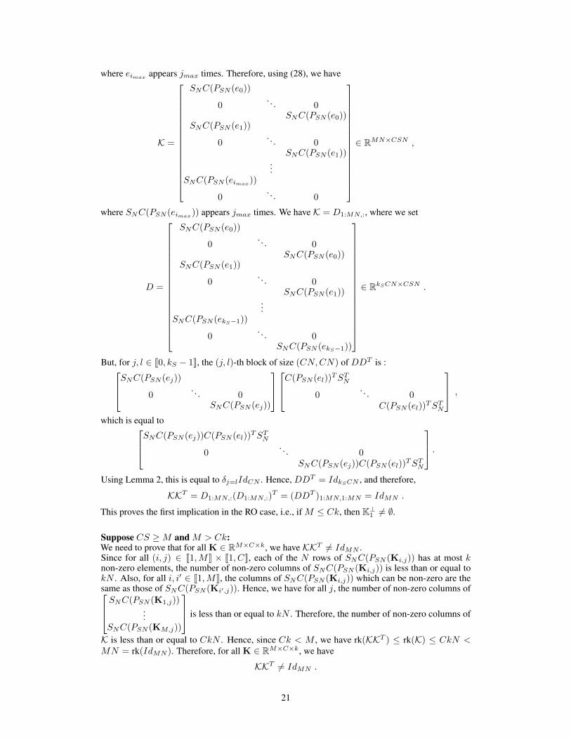
where eimax appears jmax times. Therefore, using (28), we have
K =
SNC(PSN (e0))
0. . . 0
SNC(PSN (e0))SNC(PSN (e1))
0. . . 0
SNC(PSN (e1))...
SNC(PSN (eimax))
0. . . 0
∈ RMN×CSN ,
where SNC(PSN (eimax)) appears jmax times. We have K = D1:MN,:, where we set
D =
SNC(PSN (e0))
0. . . 0
SNC(PSN (e0))SNC(PSN (e1))
0. . . 0
SNC(PSN (e1))...
SNC(PSN (ekS−1))
0. . . 0
SNC(PSN (ekS−1))
∈ RkSCN×CSN .
But, for j, l ∈ J0, kS − 1K, the (j, l)-th block of size (CN,CN) of DDT is :SNC(PSN (ej))
0. . . 0
SNC(PSN (ej))
C(PSN (el))
TSTN
0. . . 0
C(PSN (el))TST
N
,
which is equal toSNC(PSN (ej))C(PSN (el))TST
N
0. . . 0
SNC(PSN (ej))C(PSN (el))TST
N
.Using Lemma 2, this is equal to δj=lIdCN . Hence, DDT = IdkSCN , and therefore,
KKT = D1:MN,:(D1:MN,:)T = (DDT )1:MN,1:MN = IdMN .
This proves the first implication in the RO case, i.e., if M ≤ Ck, then K⊥1 6= ∅.
Suppose CS ≥M and M > Ck:We need to prove that for all K ∈ RM×C×k, we have KKT 6= IdMN .Since for all (i, j) ∈ J1,MK × J1, CK, each of the N rows of SNC(PSN (Ki,j)) has at most knon-zero elements, the number of non-zero columns of SNC(PSN (Ki,j)) is less than or equal tokN . Also, for all i, i′ ∈ J1,MK, the columns of SNC(PSN (Ki,j)) which can be non-zero are thesame as those of SNC(PSN (Ki′,j)). Hence, we have for all j, the number of non-zero columns of SNC(PSN (K1,j))
...SNC(PSN (KM,j))
is less than or equal to kN . Therefore, the number of non-zero columns of
K is less than or equal to CkN . Hence, since Ck < M , we have rk(KKT ) ≤ rk(K) ≤ CkN <MN = rk(IdMN ). Therefore, for all K ∈ RM×C×k, we have
KKT 6= IdMN .
21
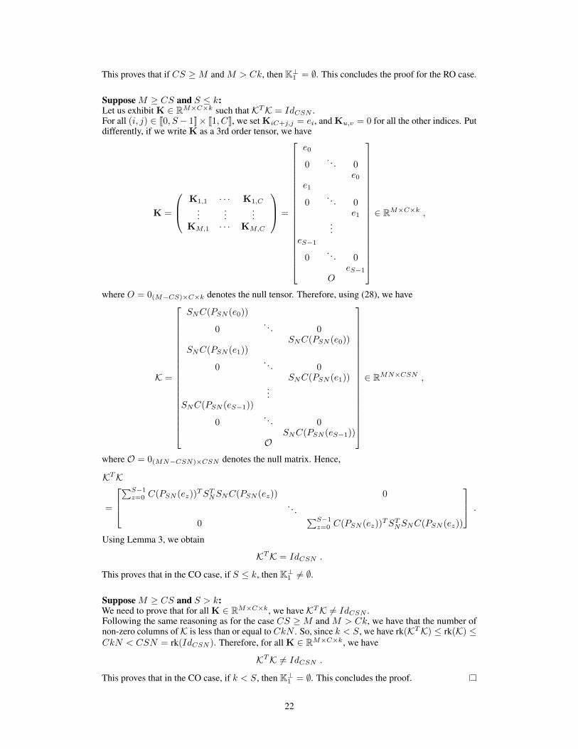
This proves that if CS ≥M and M > Ck, then K⊥1 = ∅. This concludes the proof for the RO case.
Suppose M ≥ CS and S ≤ k:Let us exhibit K ∈ RM×C×k such that KTK = IdCSN .For all (i, j) ∈ J0, S − 1K× J1, CK, we set KiC+j,j = ei, and Ku,v = 0 for all the other indices. Putdifferently, if we write K as a 3rd order tensor, we have
K =
K1,1 · · · K1,C
......
...KM,1 · · · KM,C
=
e0
0. . . 0
e0
e1
0. . . 0
e1
...eS−1
0. . . 0
eS−1
O
∈ RM×C×k ,
where O = 0(M−CS)×C×k denotes the null tensor. Therefore, using (28), we have
K =
SNC(PSN (e0))
0. . . 0
SNC(PSN (e0))SNC(PSN (e1))
0. . . 0
SNC(PSN (e1))...
SNC(PSN (eS−1))
0. . . 0
SNC(PSN (eS−1))O
∈ RMN×CSN ,
where O = 0(MN−CSN)×CSN denotes the null matrix. Hence,
KTK
=
∑S−1
z=0 C(PSN (ez))TSTNSNC(PSN (ez)) 0
. . .0
∑S−1z=0 C(PSN (ez))TST
NSNC(PSN (ez))
.
Using Lemma 3, we obtain
KTK = IdCSN .
This proves that in the CO case, if S ≤ k, then K⊥1 6= ∅.
Suppose M ≥ CS and S > k:We need to prove that for all K ∈ RM×C×k, we have KTK 6= IdCSN .Following the same reasoning as for the case CS ≥M and M > Ck, we have that the number ofnon-zero columns ofK is less than or equal to CkN . So, since k < S, we have rk(KTK) ≤ rk(K) ≤CkN < CSN = rk(IdCSN ). Therefore, for all K ∈ RM×C×k, we have
KTK 6= IdCSN .
This proves that in the CO case, if k < S, then K⊥1 = ∅. This concludes the proof.
22
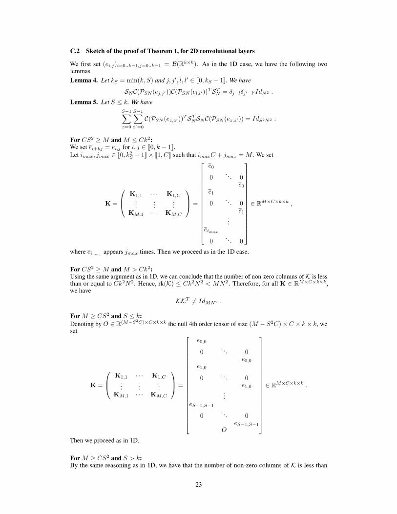
C.2 Sketch of the proof of Theorem 1, for 2D convolutional layers
We first set (ei,j)i=0..k−1,j=0..k−1 = B(Rk×k). As in the 1D case, we have the following twolemmasLemma 4. Let kS = min(k, S) and j, j′, l, l′ ∈ J0, kS − 1K. We have
SNC(PSN (ej,j′))C(PSN (el,l′))TSTN = δj=lδj′=l′IdN2 .
Lemma 5. Let S ≤ k. We haveS−1∑z=0
S−1∑z′=0
C(PSN (ez,z′))TSTNSNC(PSN (ez,z′)) = IdS2N2 .
For CS2 ≥M and M ≤ Ck2:We set ei+kj = ei,j for i, j ∈ J0, k − 1K.Let imax, jmax ∈ J0, k2
S − 1K× J1, CK such that imaxC + jmax = M . We set
K =
K1,1 · · · K1,C
......
...KM,1 · · · KM,C
=
e0
0. . . 0
e0
e1
0. . . 0
e1
...eimax
0. . . 0
∈ RM×C×k×k ,
where eimaxappears jmax times. Then we proceed as in the 1D case.
For CS2 ≥M and M > Ck2:Using the same argument as in 1D, we can conclude that the number of non-zero columns of K is lessthan or equal to Ck2N2. Hence, rk(K) ≤ Ck2N2 < MN2. Therefore, for all K ∈ RM×C×k×k,we have
KKT 6= IdMN2 .
For M ≥ CS2 and S ≤ k:Denoting by O ∈ R(M−S2C)×C×k×k the null 4th order tensor of size (M − S2C)×C × k × k, weset
K =
K1,1 · · · K1,C
......
...KM,1 · · · KM,C
=
e0,0
0. . . 0
e0,0
e1,0
0. . . 0
e1,0
...eS−1,S−1
0. . . 0
eS−1,S−1
O
∈ RM×C×k×k .
Then we proceed as in 1D.
For M ≥ CS2 and S > k:By the same reasoning as in 1D, we have that the number of non-zero columns of K is less than
23
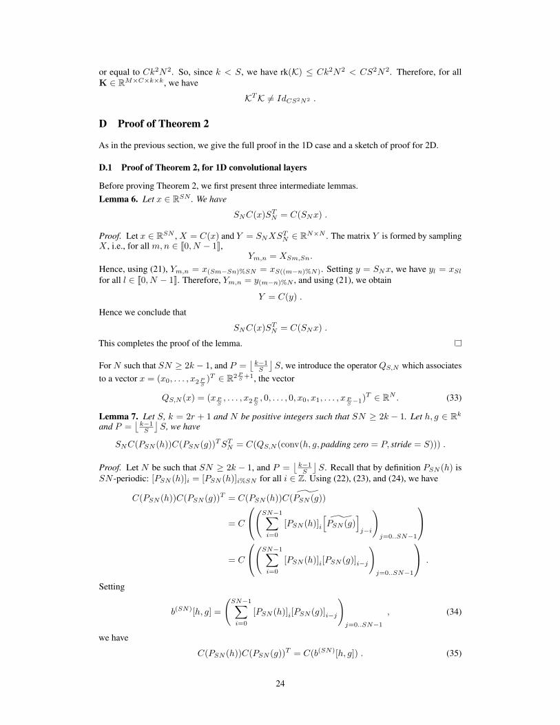
or equal to Ck2N2. So, since k < S, we have rk(K) ≤ Ck2N2 < CS2N2. Therefore, for allK ∈ RM×C×k×k, we have
KTK 6= IdCS2N2 .
D Proof of Theorem 2
As in the previous section, we give the full proof in the 1D case and a sketch of proof for 2D.
D.1 Proof of Theorem 2, for 1D convolutional layers
Before proving Theorem 2, we first present three intermediate lemmas.Lemma 6. Let x ∈ RSN . We have
SNC(x)STN = C(SNx) .
Proof. Let x ∈ RSN , X = C(x) and Y = SNXSTN ∈ RN×N . The matrix Y is formed by sampling
X , i.e., for all m,n ∈ J0, N − 1K,Ym,n = XSm,Sn.
Hence, using (21), Ym,n = x(Sm−Sn)%SN = xS((m−n)%N). Setting y = SNx, we have yl = xSl
for all l ∈ J0, N − 1K. Therefore, Ym,n = y(m−n)%N , and using (21), we obtain
Y = C(y) .
Hence we conclude that
SNC(x)STN = C(SNx) .
This completes the proof of the lemma.
For N such that SN ≥ 2k − 1, and P =⌊k−1S
⌋S, we introduce the operator QS,N which associates
to a vector x = (x0, . . . , x2 PS
)T ∈ R2 PS +1, the vector
QS,N (x) = (xPS, . . . , x2 P
S, 0, . . . , 0, x0, x1, . . . , xP
S−1)T ∈ RN . (33)
Lemma 7. Let S, k = 2r + 1 and N be positive integers such that SN ≥ 2k − 1. Let h, g ∈ Rk
and P =⌊k−1S
⌋S, we have
SNC(PSN (h))C(PSN (g))TSTN = C(QS,N (conv(h, g, padding zero = P, stride = S))) .
Proof. Let N be such that SN ≥ 2k − 1, and P =⌊k−1S
⌋S. Recall that by definition PSN (h) is
SN -periodic: [PSN (h)]i = [PSN (h)]i%SN for all i ∈ Z. Using (22), (23), and (24), we have
C(PSN (h))C(PSN (g))T = C(PSN (h))C(PSN (g))
= C
(SN−1∑i=0
[PSN (h)]i
[PSN (g)
]j−i
)j=0..SN−1
= C
(SN−1∑i=0
[PSN (h)]i[PSN (g)]i−j
)j=0..SN−1
.
Setting
b(SN)[h, g] =
(SN−1∑i=0
[PSN (h)]i[PSN (g)]i−j
)j=0..SN−1
, (34)
we have
C(PSN (h))C(PSN (g))T = C(b(SN)[h, g]) . (35)
24

To simplify the forthcoming calculations, we temporarily denote by b := b(SN)[h, g]. Notice that bydefinition, b is SN -periodic. From the definition of PSN in (26), we have, for i ∈ J−r,−r+SN−1K,
[PSN (h)]i =
{hr−i if i ∈ J−r, rK0 if i ∈ Jr + 1,−r + SN − 1K . (36)
Hence, since PSN (h) and PSN (g) are periodic, we have
bj =
SN−1∑i=0
[PSN (h)]i[PSN (g)]i−j
=
SN−1−r∑i=−r
[PSN (h)]i[PSN (g)]i−j
=
r∑i=−r
[PSN (h)]i[PSN (g)]i−j . (37)
The signal b is SN -periodic. Therefore, we can restrict the study to an interval of size SN .We consider j ∈ J−2r, SN − 2r − 1K. For any j, the set of indices i ∈ J−r, rK such that[PSN (h)]i[PSN (g)]i−j 6= 0 is included in J−r, rK ∩ {i|(i− j)%SN ∈ J−r, rK%SN}.Let j ∈ J−2r, SN − 2r − 1K: We have −r ≤ i ≤ r and −2r ≤ j ≤ SN − 2r − 1, then−SN + r + 1 ≤ i− j ≤ 3r, but by hypothesis, SN ≥ 2k − 1 = 4r + 1, hence 3r < SN − r andso −SN + r < i− j < SN − r. Therefore, for i ∈ J−r, rK and j ∈ J−2r, SN − 2r − 1K
(i− j)%SN ∈ (J−r, rK%SN) ⇐⇒ i− j ∈ J−r, rK ⇐⇒ i ∈ J−r + j, r + jK.Hence, for j ∈ J−2r, SN−2r−1K, the set of indices i ∈ J−r, rK such that [PSN (h)]i[PSN (g)]i−j 6=0 is included in J−r, rK ∩ J−r + j, r + jK.Using (10), we denote by
a = conv(h, g, padding zero = k − 1, stride = 1) ∈ R2k−1.
We have from (11), for j ∈ J0, 2k − 2K,
aj =
k−1∑i=0
higi+j .
Using (12) and keeping the indices i ∈ J0, k − 1K for which gi+j 6= 0, i.e. such that i + j ∈Jk − 1, 2k − 2K, , we obtain
{aj =
∑k−1i=k−1−j higi+j−(k−1) if j ∈ J0, k − 2K ,
aj =∑2k−2−j
i=0 higi+j−(k−1) if j ∈ Jk − 1, 2k − 2K .(38)
In the sequel, we will connect b with a by distinguishing several cases depending on the value of j.We distinguish j ∈ J0, 2rK, j ∈ J−2r,−1K and j ∈ J2r+ 1,−2r+SN − 1K. Recall that k = 2r+ 1.
If j ∈ J0, 2rK: then J−r, rK∩ J−r+ j, r+ jK = J−r+ j, rK. Using (36), the equality (37) becomes
bj =
r∑i=−r+j
[PSN (h)]i[PSN (g)]i−j
=
r∑i=−r+j
hr−igr−i+j .
By changing the variable l = r − i, and using k = 2r + 1, we find
bj =
2r−j∑l=0
hlgl+j
=
k−1−j∑l=0
hlgl+j
=
2k−2−(k−1+j)∑l=0
hlgl+(k−1+j)−(k−1) .
25
When j ∈ J0, 2rK = J0, k− 1K, we have k− 1 + j ∈ Jk− 1, 2k− 2K, therefore using (38), we obtain
bj = ak−1+j . (39)
If j ∈ J−2r,−1K: then J−r, rK ∩ J−r + j, r + jK = J−r, r + jK. Using (36), the equality (37)becomes
bj =
r+j∑i=−r
[PSN (h)]i[PSN (g)]i−j
=
r+j∑i=−r
hr−igr−i+j .
By changing the variable l = r − i, and using k = 2r + 1, we find
bj =
2r∑l=−j
hlgl+j
=
k−1∑l=−j
hlgl+j
=
k−1∑l=k−1−(k−1+j)
hlgl+(k−1+j)−(k−1) .
When j ∈ J−2r,−1K = J−(k − 1),−1K, we have k − 1 + j ∈ J0, k − 2K, and using (38), we obtain
bj = ak−1+j . (40)
If j ∈ J2r + 1, SN − 2r − 1K: then J−r, rK ∩ J−r + j, r + jK = ∅. The equality (37) becomes
bj = 0. (41)
Therefore, we summarize (39), (40) and (41): For all j ∈ J−(k − 1),−(k − 1) + SN − 1K,
bj =
{ak−1+j if j ∈ J−(k − 1), k − 1K,0 if j ∈ Jk, SN − kK. (42)
Recall that P =⌊k−1S
⌋S ≤ k − 1, and let i ∈ J0, 2P K. Therefore i − P ∈ J−P, P K ⊂ J−(k −
1), k − 1K, hence using (13) and (42), we have
[conv(h, g, padding zero = P, stride = 1)]i = ak−1+i−P = bi−P .
Therefore, using (14),
conv(h, g, padding zero = P, stride = S) =
b−b k−1S cS...
b−2S
b−Sb0bSb2S
...bb k−1
S cS
∈ R2P/S+1 . (43)
26

Using the definition of QS,N in (33), we obtain
QS,N (conv(h, g, padding zero = P, stride = S)) =
b0bSb2S
...bb k−1
S cS0...0
b−b k−1S cS...
b−2S
b−S
∈ RN .
But, using (41), and since⌊k−1S
⌋S is the largest multiple of S less than or equal to k − 1, we have
SNb =
b0bSb2S
...bb k−1
S cS0...0
bSN−b k−1S cS
...bSN−2S
bSN−S
=
b0bSb2S
...bb k−1
S cS0...0
b−b k−1S cS...
b−2S
b−S
∈ RN .
Finally, we have
SNb = QS,N (conv(h, g, padding zero = P, stride = S)) .
Using (35) and Lemma 6, we conclude that
SNC(PSN (h))C(PSN (g))TSTN = SNC(b(SN)[h, g])ST
N
= C(SNb(SN)[h, g])
= C(QS,N (conv(h, g, padding zero = P, stride = S))) .
Lemma 8. Let M , C, S, k = 2r + 1 be positive integers, and let K ∈ RM×C×k. Let N be such
that SN ≥ 2k − 1, and P =⌊k−1S
⌋S. We denote by zP/S =
0P/S
10P/S
∈ R2P/S+1. We have
KKT − IdMN =
C(QS,N (x1,1)) . . . C(QS,N (x1,M ))...
. . ....
C(QS,N (xM,1)) . . . C (QS,N (xM,M ))
,
where for all m, l ∈ J1,MK,
xm,l =
C∑c=1
conv(Km,c,Kl,c, padding zero = P, stride = S)− δm=lzP/S ∈ R2P/S+1 . (44)
27

Proof. We have from (28),
K =
SNC(PSN (K1,1)) . . . SNC(PSN (K1,C))...
......
SNC(PSN (KM,1)) . . . SNC(PSN (KM,C))
∈ RMN×CSN .
Hence, we have that the block (m, l) ∈ J1,MK2 of size (N,N) of KKT is equal to :
( SNC(PSN (Km,1)) . . . SNC(PSN (Km,C)) )
C(PSN (Kl,1))TSTN
...C(PSN (Kl,C))TST
N
=
C∑c=1
SNC(PSN (Km,c))C(PSN (Kl,c))TST
N .
We denote by Am,l the block (m, l) ∈ J1,MK2 of size (N,N) of KKT − IdMN . We want to provethat Am,l = C(QS,N (xm,l)) where xm,l is defined in (44). Using (6), (20), and (33), we have
IdN = C
([1
0N−1
])= C(QS,N (zP/S)), and therefore,
Am,l =
C∑c=1
SNC(PSN (Km,c))C(PSN (Kl,c))TST
N − δm=lC(QS,N (zP/S)) .
Using Lemma 7, this becomes
Am,l =
C∑c=1
C(QS,N (conv(Km,c,Kl,c, padding zero = P, stride = S)))− δm=lC(QS,N (zP/S)) .
By linearity of C and QS,N , we obtain
Am,l = C
(QS,N
(C∑
c=1
conv(Km,c,Kl,c, padding zero = P, stride = S)− δm=lzP/S
)).
Proof of Theorem 2. Let M , C, S, k = 2r + 1 be positive integers, and let K ∈ RM×C×k. Let Nbe such that SN ≥ 2k − 1, and P =
⌊k−1S
⌋S. For all m, l ∈ J1,MK, we denote by Am,l ∈ RN×N
the block (m, l) of KKT − IdMN . Using Lemma 8, we have
Am,l = C
(QS,N
(C∑
c=1
conv(Km,c,Kl,c, padding zero = P, stride = S)− δm=lzP/S
)).
Hence, from (20) and (33), using the fact that for all x ∈ RN , ‖C(x)‖2F = N‖x‖22, and for allx ∈ R2P/S+1, ‖QS,N (x)‖22 = ‖x‖22, we have
‖KKT − IdMN‖2F
=
M∑m=1
M∑l=1
‖Am,l‖2F
=
M∑m=1
M∑l=1
∥∥∥∥∥C(QS,N
(C∑
c=1
conv(Km,c,Kl,c, padding zero = P, stride = S)− δm=lzP/S
))∥∥∥∥∥2
F
=
M∑m=1
M∑l=1
N
∥∥∥∥∥QS,N
(C∑
c=1
conv(Km,c,Kl,c, padding zero = P, stride = S)− δm=lzP/S
)∥∥∥∥∥2
2
= N
M∑m=1
M∑l=1
∥∥∥∥∥C∑
c=1
conv(Km,c,Kl,c, padding zero = P, stride = S)− δm=lzP/S
∥∥∥∥∥2
2
.
28
Therefore, using (16) and (15), we obtain for any M , C, S, k = 2r + 1 and K ∈ RM×C×k,
‖KKT − IdMN‖2F = N‖ conv(K,K, padding zero = P, stride = S)− Ir0‖2F . (45)
This concludes the proof in the RO case.In order to prove the theorem in the CO case we use Lemma 1 in [41],
‖KTK − IdCSN‖2F = ‖KKT − IdMN‖2F + CSN −MN.
Therefore, using that (45) holds for all M , C and S, we have
‖KTK − IdCSN‖2F = N(‖ conv(K,K, padding zero = P, stride = S)− Ir0‖2F − (M − CS)
)(46)
Hence, using the definitions of errFN and Lorth in Section A.2.1, (45) and (46) lead to(errFN (K)
)2= NLorth(K).
This concludes the proof.
D.2 Sketch of the proof of Theorem 2, for 2D convolutional layers
We start by stating intermediate lemmas. First we introduce a slight abuse of notation, for a vectorx ∈ RN2
, we denote by C(x) = C(X), where X ∈ RN×N such that Vect(X) = x.Lemma 9. Let X ∈ RSN×SN . We have
SNC(X)STN = C(SN Vect(X)).
Let QS,N be the operator which associates to a matrix x ∈ R(2P/S+1)×(2P/S+1) the matrix
xP/S,P/S · · · xP/S,2P/S 0 · · · 0 xP/S,0 · · · xP/S,P/S−1
......
......
......
......
...x2P/S,P/S · · · x2P/S,2P/S 0 · · · 0 x2P/S,0 · · · x2P/S,P/S−1
0 . . . 0 0 . . . 0 0 . . . 0...
......
......
......
......
0 . . . 0 0 . . . 0 0 . . . 0x0,P/S · · · x0,2P/S 0 · · · 0 x0,0 · · · x0,P/S−1
......
......
......
......
...xP/S−1,P/S · · · xP/S−1,2P/S 0 · · · 0 xP/S−1,0 · · · xP/S−1,P/S−1
∈ RN×N .
Lemma 10. Let N be such that SN ≥ 2k − 1, h, g ∈ Rk×k and P =⌊k−1S
⌋S, we have
SNC(PSN (h))C(PSN (g))TSTN = C(QS,N (conv(h, g, padding zero = P, stride = S))) .
Lemma 11. Let M , C, S, k = 2r + 1 be positive integers, and let K ∈ RM×C×k×k. Let N besuch that SN ≥ 2k − 1, and P =
⌊k−1S
⌋S. We set zP/S,P/S ∈ R2P/S+1×2P/S+1 such that for all
i, j ∈ J0, 2P/SK, [zP/S,P/S ]i,j
= δi=P/Sδj=P/S . We have
KKT − IdMN2 =
C(QS,N (x1,1)) . . . C(QS,N (x1,M ))...
. . ....
C(QS,N (xM,1)) . . . C(QS,N (xM,M ))
,
where for all m, l ∈ J1,MK,
xm,l =
C∑c=1
conv(Km,c,Kl,c, padding zero = P, stride = S)− δm=lzP/S,P/S .
Then we proceed as in the 1D case.
29

E Proof of Theorem 3
E.1 Proof of Theorem 3, for 1D convolutional layers
Let N be a positive integer such that SN ≥ k.RO case (M ≤ CS): We denote by P =
⌊k−1S
⌋S. From Lemma 8, we have
KKT − IdMN =
C(QS,N (x1,1)) . . . C(QS,N (x1,M ))...
. . ....
C(QS,N (xM,1)) . . . C(QS,N (xM,M ))
, (47)
where for all m, l ∈ J1,MK,
xm,l =
C∑c=1
conv(Km,c,Kl,c, padding zero = P, stride = S)− δm=lzP/S ∈ R2P/S+1 . (48)
We set
B = KKT − IdMN .
SinceB is symmetric and due to the well-known properties of matrix norms, we have ‖B‖1 = ‖B‖∞and ‖B‖22 ≤ ‖B‖1‖B‖∞. Hence, using the definition of ‖B‖1, we have
‖B‖22 ≤ ‖B‖1‖B‖∞= ‖B‖21
=
(max
1≤l≤MN
MN∑m=1
|Bm,l|
)2
.
Using (47), and (20), we obtain
‖B‖22 ≤ max1≤l≤M
(M∑
m=1
‖QS,N (xm,l)‖1
)2
.
Given the definition of QS,N in (33), we have for all x ∈ R2P/S+1, ‖QS,N (x)‖1 = ‖x‖1, therefore,
‖B‖22 ≤ max1≤l≤M
(M∑
m=1
‖xm,l‖1
)2
.
We set l0 = arg max1≤l≤M
(∑Mm=1 ‖xm,l‖1
)2
. Using that for all x ∈ Rn, ‖x‖1 ≤√n‖x‖2, we
have
‖B‖22 ≤
(M∑
m=1
‖xm,l0‖1
)2
≤ (2P/S + 1)
(M∑
m=1
‖xm,l0‖2
)2
.
Using Cauchy-Schwarz inequality, we obtain
‖B‖22 ≤ (2P/S + 1)M
M∑m=1
‖xm,l0‖22
≤ (2P/S + 1)M
M∑m=1
M∑l=1
‖xm,l‖22 .
30

Using (48), then (16) and (15), we obtain
‖B‖22
≤ (2P/S + 1)M
M∑m=1
M∑l=1
∥∥∥∥∥C∑
c=1
conv(Km,c,Kl,c, padding zero = P, stride = S)− δm=lzP/S
∥∥∥∥∥2
2
= (2P/S + 1)M
M∑m=1
M∑l=1
∥∥∥[conv(K,K, padding zero = P, stride = S)− Ir0]m,l,:
∥∥∥2
2
= (2P/S + 1)M ‖conv(K,K, padding zero = P, stride = S)− Ir0‖2F= (2P/S + 1)MLorth(K) .
This proves the inequality in the RO case.
CO case (M ≥ CS): First, for n ≥ 2k − 1, let Rn be the operator that associates to x ∈ R2k−1,the vector
Rn(x) = (xk−1, . . . , x2k−2, 0, . . . , 0, x0, . . . , xk−2)T ∈ Rn . (49)
Note that, when S′ = 1, N ′ = SN , we have in (33), P ′ = k − 1 and
Q1,SN = RSN . (50)
Recall from (6) that (fi)i=0..SN−1 is the canonical basis of RSN . Let
Λj = C(fj) ∈ RSN×SN
be the permutation matrix which shifts down (cyclically) any vector by j ∈ J0, SN − 1K: for allx ∈ RSN , for i ∈ J0, SN − 1K, (Λjx)i = x(i−j)%SN . Note that, using (20), we have for allx ∈ RSN ,
[C(x)]:,j = Λjx. (51)
Recall that k = 2r + 1, and for all h ∈ Rk,
PSN (x) = (hr, . . . , h0, 0, . . . , 0, h2r, . . . , hr+1)T ∈ RSN .
For j ∈ J0, SN − 1K, for x ∈ Rk, we denote by
P(j)SN (x) = ΛjPSN (x) (52)
and for x ∈ R2k−1, we denote by
R(j)SN (x) = ΛjRSN (x). (53)
By assumption SN ≥ 2k − 1, hence RSN (x) is well-defined and we have for all j ∈ J0, SN − 1K,for all x ∈ R2k−1, {
‖R(j)SN (x)‖1 = ‖x‖1,
‖R(j)SN (x)‖2 = ‖x‖2.
(54)
We first start by introducing the following Lemma.Lemma 12. Let h, g ∈ Rk. There exist S vectors x0, . . . , xS−1 ∈ R2k−1 such that for all Nsatisfying SN ≥ 2k − 1, we have for all j ∈ J0, SN − 1K,[
C(PSN (h))TSTNSNC(PSN (g))
]:,j
= R(j)SN (xj%S) .
Proof. Recall that from (17) and (19), we have SN =∑N−1
i=0 Ei,Si and AN := STNSN =∑N−1
i=0 FSi,Si. When applied to a vector x ∈ RSN , AN keeps the elements of x with index multipleof S unchanged, while the other elements of Ax equal to zero. We know from (51) and (52) that,for j ∈ J0, SN − 1K, the j-th column of C(PSN (g)) is equal to P (j)
SN (g). Therefore, when applying
31
AN , this becomes ANP(j)SN (g) = P
(j)SN
(gj), where gj ∈ Rk is formed from g by putting zeroes in
the place of the elements that have been replaced by 0 when applying AN . But since AN keepsthe elements of index multiple of S, we have that the j-th column of ANC(PSN (g)) has the sameelements as its j%S-th column, shifted down (j − j%S) indices. This implies that gj = gj%S . Notethat we can also derive the exact formula of gj , in fact for all i ∈ J0, 2rK,[
gj]i
=
{gi if (i− r − j)%S = 00 otherwise.
We again can see that gj = gj%S . Therefore, [ANC(PSN (g))]:,j = P(j)SN
(gj%S
). Using (51)
and (52), this becomes [ANC(PSN (g))]:,j =[C(PSN
(gj%S
))]:,j
. Therefore, we have, for allj ∈ J0, SN − 1K,
[C(PSN (h))TANC(PSN (g))]:,j = C(PSN (h))TP(j)SN (gj%S)
=[C(PSN (h))TC(PSN (gj%S))
]:,j
.
Using the fact that the transpose of a circulant matrix is a circulant matrix and that two circulantmatrices commute with each other (see (22) and (25)), we conclude that the transpose of any circulantmatrix commutes with any circulant matrix, therefore
[C(PSN (h))TANC(PSN (g))]:,j =[C(PSN (gj%S))C(PSN (h))T
]:,j
.
Using Lemma 7 with S′ = 1 and N ′ = SN , and noting that,when S′ = 1, the sampling matrix SN ′
is equal to the identity, we have
C(PSN (gj%S))C(PSN (h))T
= IdN ′C(PN ′(gj%S))C(PN ′(h))T IdTN ′
= C(QS′,N ′(conv(gj%S , h, padding zero =
⌊k − 1
S′
⌋S′, stride = S′)))
= C(Q1,SN (conv(gj%S , h, padding zero = k − 1, stride = 1)))
To simplify, we denote by xj%S = conv(gj%S , h, padding zero = k − 1, stride = 1) ∈ R2k−1.Using (50), we obtain
C(PSN (gj%S))C(PSN (h))T = C(Q1,SN (xj%S))
= C(RSN (xj%S)) .
Using (51) and (53), we obtain
[C(PSN (h))TANC(PSN (g))]:,j = [C(RSN (xj%S))]:,j= ΛjRSN (xj%S)
= R(j)SN (xj%S).
Therefore, we have for all j ∈ J0, SN − 1K,[C(PSN (h))TST
NSNC(PSN (g))]:,j
= R(j)SN (xj%S) .
This concludes the proof of the lemma.
Let us go back to the main proof.
Using (28), we have that the block (c, c′) ∈ J1, CK2 of size (SN, SN) of KTK is equal to :
(C(PSN (K1,c))
TSTN . . . C(PSN (KM,c))
TSTN
) SNC(PSN (K1,c′))...
SNC(PSN (KM,c′))
=
M∑m=1
C(PSN (Km,c))TST
NSNC(PSN (Km,c′)) . (55)
32
For any (m, c, c′) ∈ J1,MK × J1, CK2, we denote by (xm,c,c′,s)s=0..S−1 ∈ R2k−1 the vectorsobtained when applying Lemma 12 with h = Km,c, and g = Km,c′ . Hence, we have, for allj ∈ J0, SN − 1K,
[C(PSN (Km,c))TST
NSNC(PSN (Km,c′))]:,j = R(j)SN (xm,c,c′,j%S) . (56)
Let fk−1 =
[0k−1
10k−1
]∈ R2k−1. For all s ∈ J0, S − 1K, we denote by
xc,c′,s =
M∑m=1
xm,c,c′,s − δc=c′fk−1 ∈ R2k−1. (57)
Note that, from (6), (49), and (53), we have for all j ∈ J0, SN − 1K, fj = R(j)SN (fk−1).
Therefore, IdSN = (f0, . . . , fSN−1) =(R
(0)SN (fk−1), . . . , R
(SN−1)SN (fk−1)
). We denote by
ANc,c′ ∈ RSN×SN the block (c, c′) ∈ J1, CK2 of KTK − IdCSN . Using (55), (56), and (57),
we have, for all j ∈ J0, SN − 1K,[AN
c,c′]:,j
=
[M∑
m=1
C(PSN (Km,c))TST
NSNC(PSN (Km,c′))− δc=c′IdSN
]:,j
=
M∑m=1
R(j)SN (xm,c,c′,j%S)− δc=c′R
(j)SN (fk−1)
= R(j)SN (xc,c′,j%S) . (58)
We set
BN = KTK − IdCSN .
We then proceed in the same way as in the RO case. Since BN is clearly symmetric, we have
‖BN‖22 ≤ ‖BN‖1‖BN‖∞= ‖BN‖21
=
(max
1≤j≤CSN
CSN∑i=1
|(BN )i,j |
)2
= max1≤c′≤C , 0≤j≤SN−1
(C∑
c=1
‖[AN
c,c′]:,j‖
1
)2
.
Using (58) and (54), this becomes
‖BN‖22 ≤ max1≤c′≤C , 0≤j≤SN−1
(C∑
c=1
‖R(j)SN
(xc,c′,j%S
)‖
1
)2
= max1≤c′≤C , 0≤s≤S−1
(C∑
c=1
‖xc,c′,s‖1
)2
.
We set (c′0, s0) = arg max1≤c′≤C , 0≤s≤S−1
(∑Cc=1 ‖xc,c′,s‖1
)2
. Using that for all x ∈ Rn,
‖x‖1 ≤√n‖x‖2, we have
‖BN‖22 ≤
(C∑
c=1
‖xc,c′0,s0‖1
)2
≤ (2k − 1)
(C∑
c=1
‖xc,c′0,s0‖2
)2
.
33
Using Cauchy-Schwarz inequality, we obtain
‖BN‖22 ≤ (2k − 1)C
C∑c=1
‖xc,c′0,s0‖2
2
≤ (2k − 1)C
C∑c=1
C∑c′=1
S−1∑s=0
‖xc,c′,s‖22 .
Using (54) in the particular case of N = 2k − 1, we obtain
‖BN‖22 ≤ (2k − 1)C
C∑c=1
C∑c′=1
S−1∑s=0
‖RS(2k−1) (xc,c′,s) ‖22
= C
C∑c=1
C∑c′=1
S−1∑s=0
(2k − 1)‖RS(2k−1) (xc,c′,s) ‖22
= C
C∑c=1
C∑c′=1
S(2k−1)−1∑j=0
∥∥∥R(j)S(2k−1)
(xc,c′,j%S
)∥∥∥2
2.
Using (58) for N = 2k − 1, we obtain
‖BN‖22 ≤ CC∑
c=1
C∑c′=1
S(2k−1)−1∑j=0
∥∥∥∥[A2k−1c,c′
]:,j
∥∥∥∥2
2
= C‖B2k−1‖2F .
Using Theorem 2 for N = 2k − 1, we have ‖B2k−1‖2F = (2k − 1)Lorth(K) and we obtain
‖BN‖22 ≤ (2k − 1)CLorth(K) .
Therefore, we conclude that, in the CO case
(errsN (K))2 ≤ (2k − 1)CLorth(K) .
This concludes the proof.
E.2 Sketch of the proof of Theorem 3, for 2D convolutional layers
In the RO case, we proceed as in the 1D case.In the CO case, we first prove a lemma similar to Lemma 12, then we proceed as in the 1D case.
F Proof of Proposition 1
Below, we prove Proposition 1 for a general matrix M ∈ Ra×b. In order to obtain the statement for aconvolutional layer K ∈ RMN×CSN :In the RO case (M ≤ CS): we take M = KT , a = CSN , b = MN .In the CO case (M ≥ CS): we take M = K, a = MN , b = CSN .
Let M ∈ Ra×b such that a ≥ b. We denote by ε = ‖MTM − Idb‖2. Let x ∈ Rb, we have∣∣‖Mx‖2 − ‖x‖2∣∣ =
∣∣xTMTMx− xTx∣∣ =
∣∣xT (MTM − Idb)x∣∣ ≤ ‖xT ‖‖MTM − Idb‖2‖x‖≤ ε‖x‖2 .
Hence, for all x ∈ Rb,
(1− ε)‖x‖2 ≤ ‖Mx‖2 ≤ (1 + ε)‖x‖2 .
This also implies σmax(M)2 ≤ 1 + ε. But we know that σmax(MT ) = σmax(M), henceσmax(MT )2 ≤ 1 + ε and therefore, for all x ∈ Ra,
‖MTx‖2 ≤ (1 + ε)‖x‖2 .This proves Proposition 1.
34

G Boundary conditions comparison
We consider in this section an unstrided convolution, and we state results about other paddings andtheir limitations.Proposition 2. Let N ≥ 2k − 1. With the padding ’valid’, there exist no orthogonal convolutionallayer in the CO case.
Note that this result still holds in the 2D case, we give a proof only in the 1D.
Proof. For a single-channel convolution of kernel h ∈ Rk with ’valid’ padding, the matrix applyingthe transformation on a signal x ∈ RN has the following form:
AN (h) :=
h0 · · · h2r 0
. . . . . . . . .. . . . . . . . .
0 h0 · · · h2r
∈ R(N−k+1)×N .
Hence, for K ∈ RM×C×k, the layer transform matrix is:
K =
AN (K1,1) . . . AN (K1,C)...
......
AN (KM,1) . . . AN (KM,C)
∈ RM(N−k+1)×CN .
Suppose that KTK = IdCN , therefore the columns of K are of norm 1. Let us focus on the columnscorresponding to the first channel. To simplify, for m ∈ J1,MK we denote by a(m) := Km,1 ∈ Rk,hence
AN (K1,1)...
AN (KM,1)
=
a(1)0 · · · a
(1)2r 0
. . . . . . . . .. . . . . . . . .
0 a(1)0 · · · a
(1)2r
a(2)0 · · · a
(2)2r 0
. . . . . . . . .. . . . . . . . .
0 a(2)0 · · · a
(2)2r
......
......
......
a(M)0 · · · a
(M)2r 0
. . . . . . . . .. . . . . . . . .
0 a(M)0 · · · a
(M)2r
.
Since KTK = IdCN , we have in particular∑M
m=1
(a
(m)0
)2
= 1∑Mm=1
(a
(m)2r
)2
= 1∑2ri=0
∑Mm=1
(a
(m)i
)2
= 1 .
This is impossible. Therefore, for all K ∈ RM×C×k, we have KTK 6= IdCN .
Recall that k = 2r + 1, and that (ei)i=0..k−1 is the canonical basis of Rk (see (6)). For the zeropadding ’same’, we have the following lemma.
35

Proposition 3. Let N ≥ k. For K ∈ RM×C×k, with the zero padding ’same’ and S = 1, bothin the RO and CO case, if K is orthogonal then there exist (αm,c)m=1..M,c=1..C such that for all(m, c) ∈ J1,MK× J1, CK, Km,c = αm,cer. This is equivalent to
K =
α1,1IdN . . . α1,CIdN...
......
αM,1IdN . . . αM,CIdN
∈ RMN×CN .
Note that this result still holds in the 2D case.
Proof. For a single-channel convolution of kernel h ∈ Rk with zero padding ’same’, the matrixapplying the transformation on a signal x ∈ RN has the following form:
AN (h) :=
hr · · · h2r 0 · · · 0...
. . . . . . . . . . . ....
h0. . . . . . . . . . . . 0
0. . . . . . . . . . . . h2r
.... . . . . . . . . . . .
...0 · · · 0 h0 · · · hr
∈ RN×N .
Hence, for K ∈ RM×C×k, the matrix that applies the convolutional layer is :
K =
AN (K1,1) . . . AN (K1,C)...
......
AN (KM,1) . . . AN (KM,C)
∈ RMN×CN .
Suppose M ≤ C (RO case): If K is orthogonal, then KKT = IdMN . Let us fix m ∈ J1,MK. SinceKKT = IdMN , we have, the first row, the last row and the row of index r of the m-th block matrixof size N × CN are of norm equal to 1, i.e.
‖K(m−1)N,:‖22 = 1
‖KmN−1,:‖22 = 1
‖K(m−1)N+r,:‖22 = 1 .
To simplify the notation, for c ∈ J1, CK, we denote by a(c) := Km,c ∈ Rk, hence the previoussystem is equivalent to
∑2ri=r
∑Cc=1
(a
(c)i
)2
= 1∑ri=0
∑Cc=1
(a
(c)i
)2
= 1∑2ri=0
∑Cc=1
(a
(c)i
)2
= 1 .
Substracting the first equality from the third one, and the second equality from the third one, weobtain
∑r−1i=0
∑Cc=1
(a
(c)i
)2
= 0∑2ri=r+1
∑Cc=1
(a
(c)i
)2
= 0∑2ri=0
∑Cc=1
(a
(c)i
)2
= 1 .
This implies that for all c ∈ J1, CK, for all i ∈ J0, 2rK \ {r}, a(c)i = 0.
As a conclusion, for any m ∈ J1,MK, any c ∈ J1, CK, and any i ∈ J0, 2rK \ {r}, we haveKm,c,i = 0.
This proves the result in the RO case.The proof of the CO case is similar, and we have the same conclusion.
To recapitulate, we have proven that with padding ’valid’, no orthogonal convolution can be built in theCO case, and that for zero padding ’same’, the orthogonal convolutions lead to trivial transformation.
36
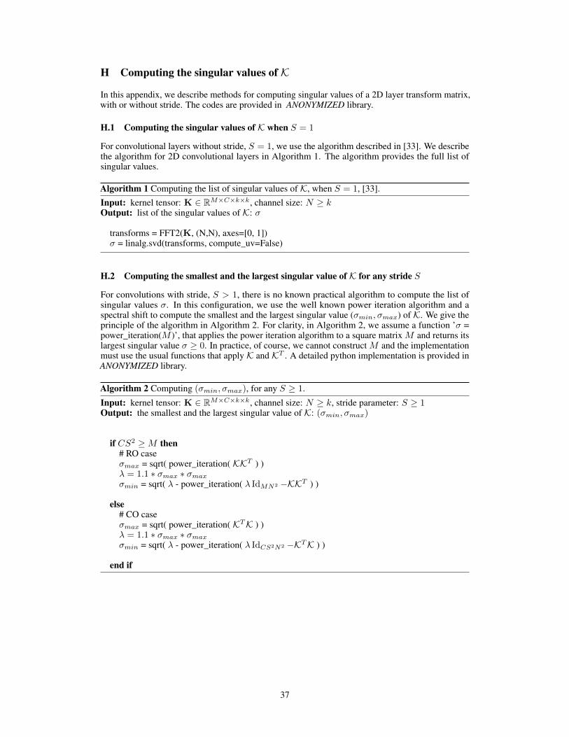
H Computing the singular values of K
In this appendix, we describe methods for computing singular values of a 2D layer transform matrix,with or without stride. The codes are provided in ANONYMIZED library.
H.1 Computing the singular values of K when S = 1
For convolutional layers without stride, S = 1, we use the algorithm described in [33]. We describethe algorithm for 2D convolutional layers in Algorithm 1. The algorithm provides the full list ofsingular values.
Algorithm 1 Computing the list of singular values of K, when S = 1, [33].Input: kernel tensor: K ∈ RM×C×k×k, channel size: N ≥ kOutput: list of the singular values of K: σ
transforms = FFT2(K, (N,N), axes=[0, 1])σ = linalg.svd(transforms, compute_uv=False)
H.2 Computing the smallest and the largest singular value of K for any stride S
For convolutions with stride, S > 1, there is no known practical algorithm to compute the list ofsingular values σ. In this configuration, we use the well known power iteration algorithm and aspectral shift to compute the smallest and the largest singular value (σmin, σmax) of K. We give theprinciple of the algorithm in Algorithm 2. For clarity, in Algorithm 2, we assume a function ’σ =power_iteration(M )’, that applies the power iteration algorithm to a square matrix M and returns itslargest singular value σ ≥ 0. In practice, of course, we cannot construct M and the implementationmust use the usual functions that apply K and KT . A detailed python implementation is provided inANONYMIZED library.
Algorithm 2 Computing (σmin, σmax), for any S ≥ 1.
Input: kernel tensor: K ∈ RM×C×k×k, channel size: N ≥ k, stride parameter: S ≥ 1Output: the smallest and the largest singular value of K: (σmin, σmax)
if CS2 ≥M then# RO caseσmax = sqrt( power_iteration( KKT ) )λ = 1.1 ∗ σmax ∗ σmax
σmin = sqrt( λ - power_iteration( λ IdMN2 −KKT ) )
else# CO caseσmax = sqrt( power_iteration( KTK ) )λ = 1.1 ∗ σmax ∗ σmax
σmin = sqrt( λ - power_iteration( λ IdCS2N2 −KTK ) )
end if
37