shapeconv: shape-aware convolutional layer for indoor

ShapeConv: Shape-aware Convolutional Layerfor Indoor RGB-D Semantic Segmentation

Jinming Cao1 Hanchao Leng1 Dani Lischinski2 Danny Cohen-Or3 Changhe Tu1* Yangyan Li4∗1Shandong University, China 2The Hebrew University of Jerusalem, Israel

3Tel Aviv University, Israel 4Alibaba Group, China{jinming.ccao, hanchao.leng, danix3d, cohenor, changhe.tu, yangyan.lee}@gmail.com

AbstractRGB-D semantic segmentation has attracted increasing

attention over the past few years. Existing methods mostlyemploy homogeneous convolution operators to consume theRGB and depth features, ignoring their intrinsic differences.In fact, the RGB values capture the photometric appearanceproperties in the projected image space, while the depth fea-ture encodes both the shape of a local geometry as well asthe base (whereabout) of it in a larger context. Comparedwith the base, the shape probably is more inherent and hasa stronger connection to the semantics, and thus is morecritical for segmentation accuracy. Inspired by this obser-vation, we introduce a Shape-aware Convolutional layer(ShapeConv) for processing the depth feature, where thedepth feature is firstly decomposed into a shape-componentand a base-component, next two learnable weights are in-troduced to cooperate with them independently, and finallya convolution is applied on the re-weighted combinationof these two components. ShapeConv is model-agnosticand can be easily integrated into most CNNs to replacevanilla convolutional layers for semantic segmentation. Ex-tensive experiments on three challenging indoor RGB-D se-mantic segmentation benchmarks, i.e., NYU-Dv2(-13,-40),SUN RGB-D, and SID, demonstrate the effectiveness of ourShapeConv when employing it over five popular architec-tures. Moreover, the performance of CNNs with ShapeConvis boosted without introducing any computation and mem-ory increase in the inference phase. The reason is thatthe learnt weights for balancing the importance betweenthe shape and base components in ShapeConv become con-stants in the inference phase, and thus can be fused into thefollowing convolution, resulting in a network that is identi-cal to one with vanilla convolutional layers.

1. IntroductionWith the widespread use of depth sensors (such as Mi-

crosoft Kinect [31]), the availability of RGB-D data has

*Corresponding Author

!"# $%&'ℎ

ℙ! ℙ" ℙ! ℙ"

ℙ# ℙ$ℙ# ℙ$

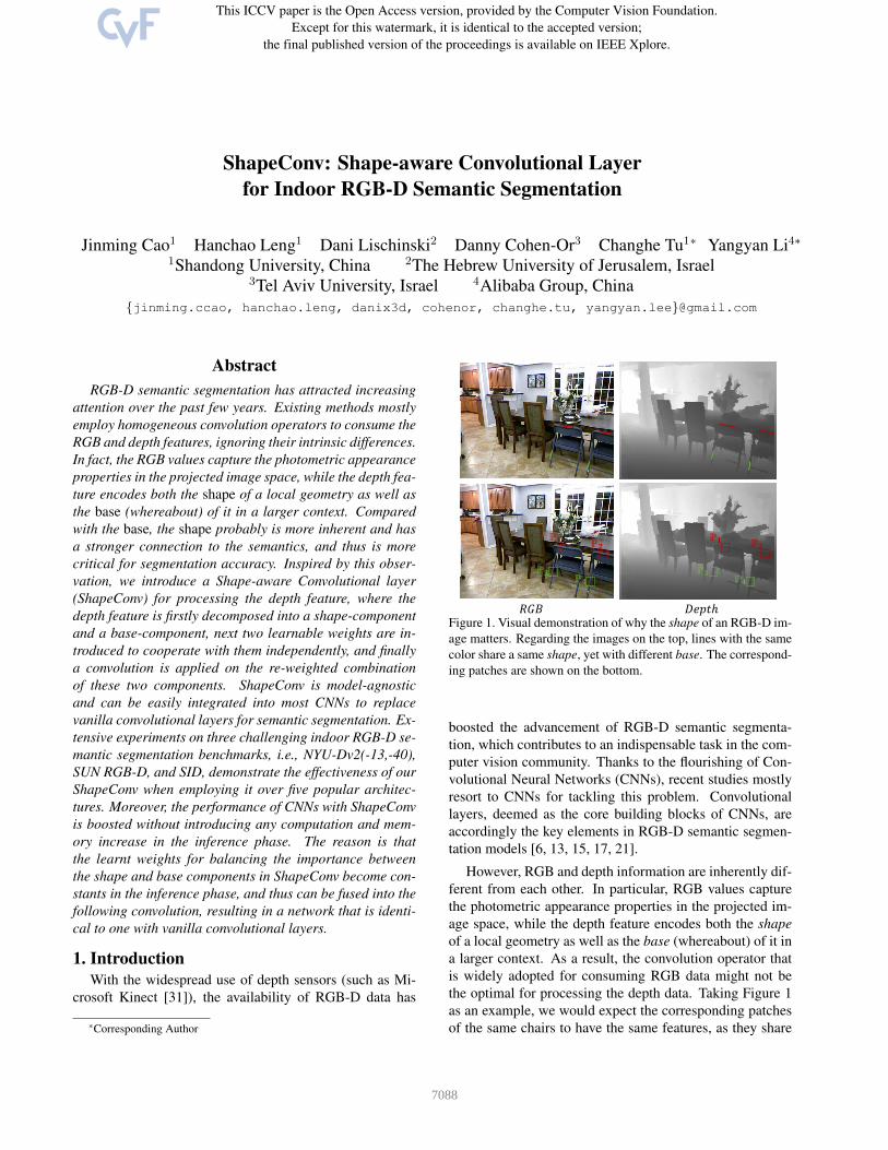
Figure 1. Visual demonstration of why the shape of an RGB-D im-age matters. Regarding the images on the top, lines with the samecolor share a same shape, yet with different base. The correspond-ing patches are shown on the bottom.

boosted the advancement of RGB-D semantic segmenta-tion, which contributes to an indispensable task in the com-puter vision community. Thanks to the flourishing of Con-volutional Neural Networks (CNNs), recent studies mostlyresort to CNNs for tackling this problem. Convolutionallayers, deemed as the core building blocks of CNNs, areaccordingly the key elements in RGB-D semantic segmen-tation models [6, 13, 15, 17, 21].

However, RGB and depth information are inherently dif-ferent from each other. In particular, RGB values capturethe photometric appearance properties in the projected im-age space, while the depth feature encodes both the shapeof a local geometry as well as the base (whereabout) of it ina larger context. As a result, the convolution operator thatis widely adopted for consuming RGB data might not bethe optimal for processing the depth data. Taking Figure 1as an example, we would expect the corresponding patchesof the same chairs to have the same features, as they share

7088

the same shape. The shape is a more inherent property ofthe underlying object and has stronger connection to the se-mantics. We would expect to achieve shape invariance inthe learning process. When a vanilla convolution operatoris applied on these corresponding patches, the resulting fea-tures are different due to the differences in their base com-ponent, hindering the learning from achieving shape invari-ance. On the other hand, the base components cannot besimply discarded for pursuing the shape invariance in thecurrent layer, as they form the shape in a followup layerwith a larger context.

To address these problems, we propose a Shape-awareConvlutional layer (ShapeConv), to learn the adaptive bal-ance between the importance of shape and base informa-tion, giving the network the chance to focus more on theshape information whenever necessary for benefiting theRGB-D semantic segmentation task. We firstly decom-pose a patch1 into two separate components, i.e., a base-component and a shape-component. The mean of patch val-ues depicts the whereabout of the patch in a larger context,thus constitutes the base component, while the residual isthe relative changes in the patch, which depicts the shapeof the underlying geometry, thus constitutes to the shapecomponent. Specifically, for an input patch (such as P1 inFigure 1), the base describes where the patch is, i.e., the dis-tance from the observation point; while the shape expresseswhat the patch is, e.g., a chair corner. We then employ twooperations, namely, base-product and shape-product, to re-spectively process these two components with two learn-able weights, i.e., base-kernel and shape-kernel. The outputfrom these two is then combined in an addition manner toform a shape-aware patch, which is further convolved witha normal convolutional kernel. In contrast to the originalpatch, the shape-aware one is capable of adaptively learn-ing the shape characteristic with the shape-kernel, and thebase-kernel serves to balance the contributions of the shapeand the base for the final prediction.

In addition, since the base-kernel and shape-kernel be-come constants in the inference phase, we can fuse theminto the following convolution kernel, resulting in a networkthat is identical to the one with vanilla convolutional layers.The proposed ShapeConv can be easily plugged into mostCNNs as a replacement of the vanilla convolution in seman-tic segmentation without introducing any computation andmemory increase in the inference phase. This simple re-placement transforms CNNs designed for RGB data intoones better suited for consuming RGB-D data.

To validate the effectiveness of the proposed method,we conduct extensive experiments on three challengingRGB-D indoor semantic segmentation benchmarks: NYU-Dv2 [25](-13,-40), SUN RGBD [26], and SID [1]. We ap-

1The operation unit of input features for the convolutional layer, whosespatial size is the same as the convolution kernel.

ply our ShapeConv to five popular semantic segmentationarchitectures and can observe promising performance im-provements compared with baseline models. We found thatShapeConv can significantly improve the segmentation ac-curacy around the object boundaries (see Figure 5), whichdemonstrates the effective leveraging of the depth informa-tion2.

2. Related WorkCNNs have been widely used for semantic segmentation

on RGB images [3, 4, 19, 18, 23, 33]. In general, exist-ing segmentation architectures usually involve two stages:the backbone and the segmentation stage. The former stageis leveraged to extract features from RGB images, whereinpopular models are ResNet [12], ResNeXt [29] which arepre-trained on the ImageNet dataset [24]. The latter stageaims to generate predictions based on the extracted features.Methods in this stage include Upsample [19], PPM [33] andASPP [3, 4], etc. It is worth noting that both stages adoptthe convolutional layers as the core building blocks.

As RGB semantic segmentation has been extensivelystudied in literature, a straightforward solution for RGB-Dsemantic segmentation is to adapt the well-developed archi-tectures from the ones designed for RGB data. However,implementing such a idea is non-trivial due to the asym-metric modality problem between the RGB and the depthinformation. To tackle this, researchers have devoted ef-forts into two directions: designing dedicated architecturesfor RGB-D data [6, 8, 13, 15, 17, 21, 28], and presentingnovel layers to enhance or replace the convolutional layersin RGB semantic segmentation [5, 27, 30]. Our method fallsinto the second category.

Methods in the first category propose to feed RGB anddepth channels to two parallel CNNs streams, where theoutput features are fused with specific strategies. For ex-ample, [6] presents a gate-fusion method, [8, 13, 21] fusethe features in multi-levels of the backbone stages. Never-theless, these methods mostly leverage separate networks toconsume RGB and depth features, they are yet faced withtwo limitations: 1) it is hard to decide when is the best stagefor the fusion to happen; and 2) the two-stream or multi-level way often results in large increase of computation.

In contrast, methods along the second direction target atdesigning novel layers based on the geometric character-istics of RGB-D data, which are more flexible and time-efficient. For instance, Wang et al. [27] proposed the depth-aware convolution to weight pixels based on a hand-craftedGaussian function by leveraging the depth similarity be-tween pixels. [30] presents a novel operator called mal-leable 2.5D convolution, to learn the receptive field alongthe depth-axis. [5] devises a S-Conv to infer the samplingoffset of the convolution kernel guided by the 3D spatial

2Our code is released through https://github.com/hanchaoleng/ShapeConv.

7089

information, enabling the convolutional layer to adjust thereceptive field and geometric transformations. ShapeConvproposed a novel view of the content in each patch and amechanism to leverage them adaptively with learnt weights.Moreover, ShapeConv can be converted into vanilla convo-lution in the inference phase, resulting in ZERO increase ofmemory and computation compared with the models withvanilla convolution.

3. MethodIn this section, we first provide the basic formulation

of the Shape-aware convolutional layer (ShapeConv) forRGB-D data, followed by its application in the training andinference phase. We end this section with the method archi-tectures.

3.1. ShapeConv for RGB-D DataMethod Intuition. Given an input patch P ∈RKh×Kw×Cin , Kh and Kw are the spatial dimen-sions of the kernel; Cin represents the channel numbers inthe input feature map, the output features from the vanillaconvolution layer are obtained by,

F = Conv(K,P), (1)

where K ∈ RKh×Kw×Cin×Cout denotes the learnableweights of kernels in a convolutional layer (The bias termsare not included for simplicity.); Cout represents the chan-nel numbers in the output feature map. Each element ofF ∈ RCout is calculated as,

Fcout=

Kh×Kw×Cin∑i

(Ki,cout × Pi).

It can be easily recognized that F usually changes withrespect to different values of P. Take the two patches in theFigure 1, P1 and P2, as an example. The corresponding out-put features, F1 and F2 from the vanilla convolution layerare learned by: F1 = Conv(K,P1), F2 = Conv(K,P2).Since P1 and P2 are not identical (different distances fromthe observation points), accordingly, their features are usu-ally different, and this may lead to distinct prediction re-sults.

Nevertheless, P1 and P2, corresponding to the red re-gions in Figure 1, actually belong to the same class - chair.And vanilla convolutional layers cannot well handle suchsituations. In fact, there exists some invariants of thesetwo patches, namely, the shape. It refers to the relativedepth correlation under local features, which is however,unexpectedly ignored by the existing methods. In view ofthis, we propose to fill this gap via effectively modeling theshape for RGB-D semantic segmentation.

ShapeConv Formulation. Based on the aforementionedanalysis, in this paper, we offer to decompose an input

patch into two components: a base-component PB describ-ing where the patch is, and a shape-component PS express-ing what the patch is. Therefore, we refer the mean3 ofpatch values to be PB , and its relative values to be as PS :

PB = m(P),PS = P−m(P),

where m(P) is the mean function on P (over the Kh ×Kw dimensions), and PB ∈ R1×1×Cin , and PS ∈RKh×Kw×Cin .

Note that directly convolved PS with K in Equation 1is sub-optimal, as the values from PB contributes the classdiscrimination across patches. Thus, our ShapeConv in-stead leverages two learnable weights, WB ∈ R1 andWS ∈ RKh×Kw×Kh×Kw×Cin , to separately consume theabove two components. The outputted features are thencombined in an element-wise addition manner, which formsa new shape-aware patch with the same size as the originalone P. The formulation of ShapeConv is given as,

F = ShapeConv(K,WB ,WS ,P)= Conv(K,WB � PB +WS ∗ PS)

= Conv(K,PB + PS)

= Conv((K,PBS),

(2)

where � and ∗ denote the base-product and shape-productoperator, respectively, which are defined as,{

PB = WB � PB

PB1,1,cin= WB × PB1,1,cin

,(3)

{PS = WS ∗ PS

PSkh,kw,cin=

∑Kh×Kw

i (WSi,kh,kw,cin× PSi,cin

),

(4)where cin, kh, kw are the indices of the elements in Cin,Kh, Kw dimensions, respectively.

We reconstruct the shape-aware patch PBS from the addi-tion of PB and PS, and PBS ∈ RKh×Kw×Cin , which enablesit to be smoothly convolved by the kernel K of vanilla con-volutional layer. Nevertheless, the PBS is equipped with theimportant shape information which is learned by the twoadditional weights, making the convolutional layer to focuson the situations when merely using depth values fails.

3.2. ShapeConv in Training and InferenceTraining phase. The proposed ShapeConv in Sec-tion 3.1 can effective leverage the shape information ofpatches. However, replacing vanilla convolutional layerwith ShapeConv in CNNs introduces more computational

3As the depth values are obtained from a fixed observation point, wenotice that the rotational transformations cannot be addressed due to theangle of view limitation. As a result, we focus more on the translationaltransformations in this paper.

7090

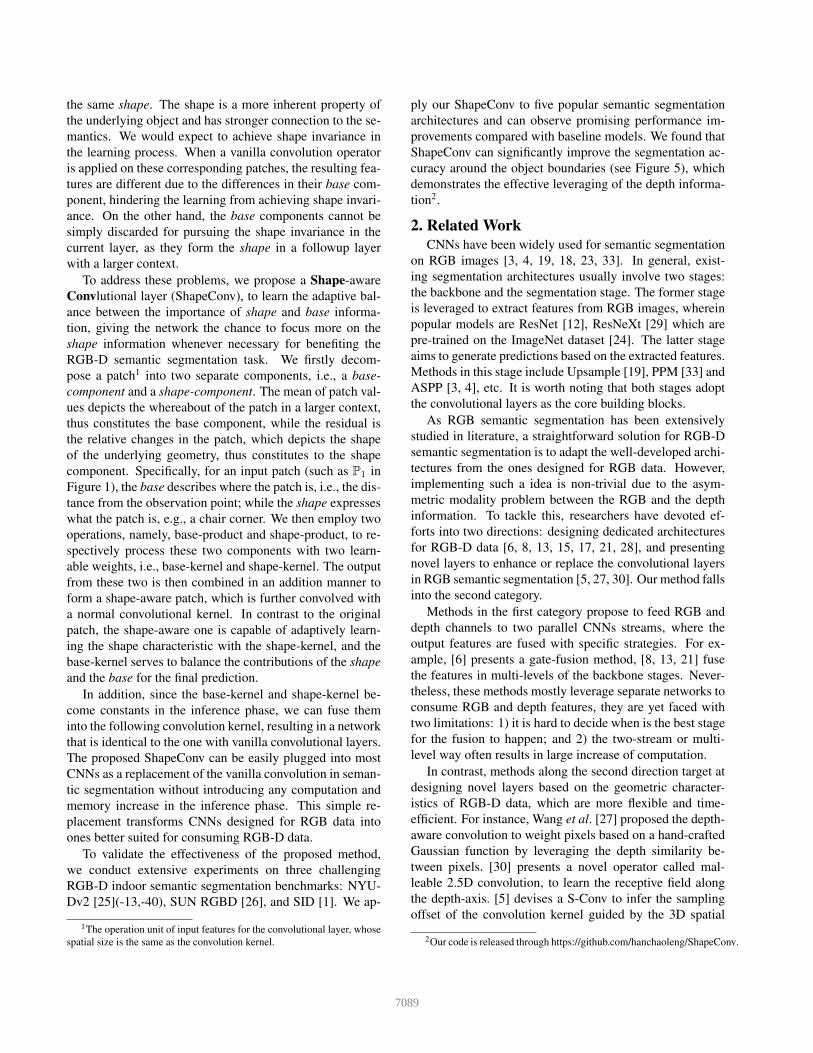
!" = 2, !# = 2, %$%= 3, %&'( = 2

! = #ℎ%&'()*+(,,.! ,.", ℙ)=()*+(0#$, ℙ)

7+,

ℙ (

% ! = ()*+(,, ℙ)

(ℙ

-

-

+

1 , +." ∗ , −1 ,5 0#$= .!

7+,

6)

6*

6* ∗ - −8 -

6) 8 -8 -

-−8 -

6

Figure 2. Comparison of vanilla convolution and ShapeConvwithin a patch P. In this figure, Kh = Kw = 2, Cin = 3, andCout = 2, “+” denotes element-wise addition. (a) Vanilla convo-lution with kernel K; (b) ShapeConv with folding the WB and WS

into KBS; (c) The computation of KBS from K, WB and WS .

cost due to the two product operation in Equation 3 and 4.To tackle this problem, we propose to shift these two oper-ations from patches to kernels,{

KB = WB �KB

KB1,1,cin,cout= WB ×KB1,1,cin,cout

,{KS = WS ∗KS

KSkh,kw,cin,cout=

∑Kh×Kw

i (WSi,kh,kw,cin×KSi,cin,cout

),

where KB ∈ R1×1×Cin×Cout and KS ∈RKh×Kw×Cin×Cout denote the base-component of kernelsand shape-component, respectively, and K = KB +KS .

We therefore re-formalize ShapeConv the Equation 2 tofollowing:

F = ShapeConv(K,WB ,WS ,P)= Conv(WB �m(K) +WS ∗ (K−m(K)),P)= Conv(WB �KB +WS ∗KS ,P)= Conv(KB + KS,P)= Conv(KBS,P),

(5)

where m(K) is the mean function on K (over the Kh×Kw

dimensions). And we require KBS = KB + KS, KBS ∈RKh×Kw×Cin×Cout .

In fact, the two formulations of ShpeConv, i.e., Equa-tion 2 and Equation 5 are mathematically equivalent, i.e.,

F = ShapeConv(K,WB ,WS ,P)= Conv(K,PBS)

= Conv(KBS,P),(6)

Fcout=

Kh×Kw×Cin∑i

(Ki,cout× PBSi

)

=

Kh×Kw×Cin∑i

(KBSi,cout× Pi),

(7)

please refer to the Supp. for detailed proof. In this way, weutilize the ShapeConv in Equation 5 in our implementationas illustrated in Figure 2(b) and (c).Inference phase. During inference, since the two addi-tional weights i.e. WB and WS , become constants, we canfuse them into KBS as shown in Figure 2(c) with KBS =WB � KB + WS ∗ KS . And KBS shares the same tensorsize with K in Equation 1, thus, our ShapeConv is actuallythe same as the vanilla convolutional layer in Figure 2(a).In other words, when replacing vanilla convolution withShapeConv, there would introduce zero additional inferencetime.

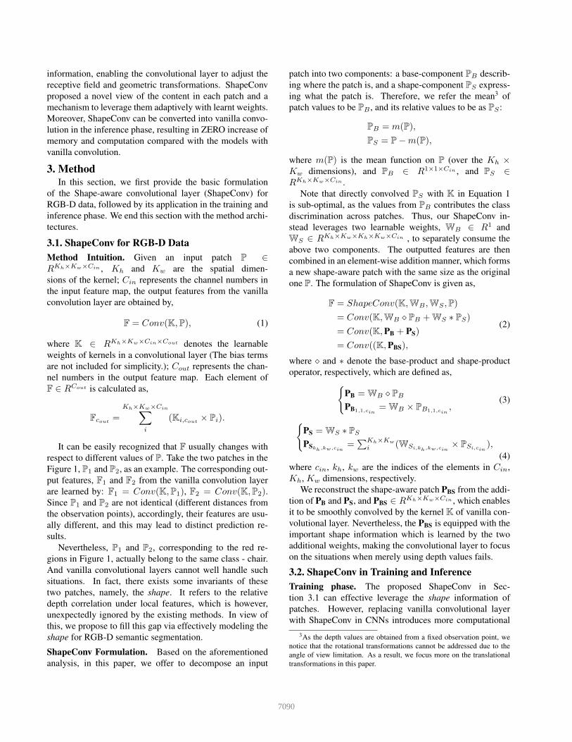
3.3. ShapeConv-enhanced Network ArchitectureDifferent from devising specially dedicated architec-

tures for RGB-D segmentation [21, 22, 17], the proposedShapeConv is a more generalized approach that can be eas-ily plugged into most CNNs as a replacement for the vanillaconvolution in semantic segmentation, which is then trans-formed for adapting the RGB-D data.

Figure 3 depicts an example of the overall method archi-tecture. In order to leverage the advanced backbones in se-mantic segmentation, we firstly require to convert the inputfeatures from RGB images to RGB-D data via the concate-nation of the RGB and D information. In practice, D canbe depth values [11, 20] or HHA4 images [10, 19, 16, 6].We then replace the vanilla convolution layer with theShapeConv in both the backbone and segmentation stages.It is worth noting that, WB is initialized to one, WS canbe viewed as Cin square (Kh ×Kw)× (Kh ×Kw) matri-ces, which are initialized to the identity matrix. In this way,ShapeConv is equivalent to the vanilla convolution at thebeginning of training since KBS = K. This initialization ap-proach offers two advantages: 1) It makes the ShapeConv-enhanced networks do not interfere with the RGB data, i.e.,the RGB features are processed in the same way as before.2) It facilitates ShapeConv to reuse the parameters from pre-trained models.

Thus, with this approach, future advances in RGB se-mantic segmentation architectures can be easily transferred

4Horizontal disparity, Height above ground and normal Angle to thevertical axis.

7091

<=5>?%@?*+(AB@4B@)

C=*B+>@=B@ℎ

)*+, E'%!0*+5 2@'F5)*+,

25F85+@'@?*+2@'F5

2ℎ'45)*+, E'%!0*+5 2@'F52ℎ'45)*+,25F85+@'@?*+

2@'F5

BaselineC

GCE

H I+4B@

Ours

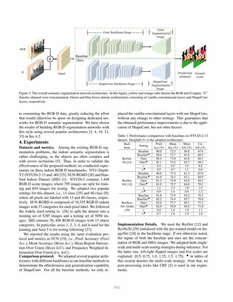
Figure 3. The overall semantic segmentation network architecture. In this figure, yellow and orange cube denote the RGB and D inputs; “C”denotes channel-wise concatenation; Green and blue boxes denote architectures consisting of vanilla convolutional layers and ShapeConvlayers, respectively.

to consuming the RGB-D data, greatly reducing the effortthat would otherwise be spent on designing dedicated net-works for RGB-D semantic segmentation. We have shownthe results of building RGB-D segmentation networks withthis style using several popular architectures [3, 4, 18, 23,33] in Sec 4.2.

4. ExperimentsDatasets and metrics. Among the existing RGB-D seg-mentation problems, the indoor semantic segmentation israther challenging, as the objects are often complex andwith severe occlusions [5]. Thus, in order to validate theeffectiveness of the proposed method, we conducted exper-iments on three indoor RGB-D benchmarks: NYU-Depth-V2 (NYUDv2-13 and -40) [25], SUN-RGBD [26] and Stan-ford Indoor Dataset (SID) [1]. NYUDv2 contains 1,449RGB-D scene images, where 795 images are split for train-ing and 654 images for testing. We adopted two popularsettings for this dataset, i.e., 13-class [25] and 40-class [9],where all pixels are labeled with 13 and 40 classes, respec-tively. SUN-RGBD is composed of 10,355 RGB-D indoorimages with 37 categories for each pixel label. We followedthe widely used setting in [26] to split the dataset into atraining set of 5285 images and a testing set of 5050 im-ages. SID contains 70, 496 RGB-D images with 13 objectcategories. In particular, areas 1, 2, 3, 4, and 6 used for thetraining and Area 5 is for testing following [27].

We reported the results using the same evaluation pro-tocol and metrics as FCN [19], i.e., Pixel Accuracy (PixelAcc.), Mean Accuracy (Mean Acc.), Mean Region Intersec-tion Over Union (Mean IoU), and Frequency Weighted In-tersection Over Union (f.w. IoU).Comparison protocol. We adopted several popular archi-tectures with different backbones as our baseline methods todemonstrate the effectiveness and generalization capabilityof ShapeConv. For all the baseline methods, we only re-

placed the vanilla convolutional layers with our ShapeConv,without any change to other settings. This guarantees thatthe obtained performance improvements is due to the appli-cation of ShapeConv, but not other factors.

Table 1. Performance comparison with baselines on NYUDv2-13dataset. Deeplabv3+ is the adopted architecture.

Back Setting Pixel Mean Mean f.w.bone Acc.(%) Acc.(%) IoU.(%) IoU.(%)

Baseline 80.0 72.5 60.8 67.6BaselineF 80.6 72.7 61.6 68.5

ResNet Ours 80.4 73.0 61.8 68.150 [12] OursF 81.1 73.4 62.7 69.1

+ 0.4 0.5 1.0 0.5+F 0.5 0.7 1.1 0.6



+ 1.2 1.5 1.6 1.5+F 0.9 1.4 0.9 1.2


ResNext Ours 82.6 75.7 65.1 71.2101 32x8d OursF 82.9 76.0 65.6 71.6

[29] + 0.8 1.8 1.9 1.1+F 0.7 1.6 1.9 1.0

Implementation Details. We used the ResNet [12] andResNeXt [29] initialized with the pre-trained model on Im-ageNet [24] in the backbone stage. If not otherwise noted,the inputs of both the baseline and ours are the concate-nation of RGB and HHA images. We adopted both single-scale and multi-scale testing strategies during inference. Forthe latter one, left-right flipped images and five scales areexploited: [0.5, 0.75, 1.0, 1.25, 1.5, 1.75]. F in tables ofthis section denotes the multi-scale strategy. Note that, nopost-processing tricks like CRF [2] is used in our experi-ments.

7092

! "

#$%&'( )* +!(,-.$, /&0( #$%&'( )* +!(,-.$, /&0(

Figure 4. Visualization results from NYUDv2 dataset. Input column denotes RGB, Depth, HHA images from top to bottom; the blackregions in the GT, Baseline and Ours indicate the ignored category. The upper and lower cases are from NYUDv2-40 and NYUDv2-13,respectively.

Table 2. Performance comparison with baselines on NYUDv2-40dataset. Deeplabv3+ is the adopted architecture.

Back Setting Pixel Mean Mean f.w.bone Acc.(%) Acc.(%) IoU.(%) IoU.(%)



+ 1.0 1.4 1.7 1.3+F 0.8 1.4 1.7 1.2



+ 1.1 0.6 1.59 1.1+F 1.1 0.5 1.4 1.0


ResNext Ours 75.8 62.8 50.2 62.6101 32x8d OursF 76.4 63.5 51.3 63.0

[29] + 1.1 1.3 1.3 1.1+F 1.0 0.9 1.0 0.8

4.1. Experiments on Different DatasetsNYUDv2 Dataset. We adopted two popular settings forthis dataset, i.e., 13-class [25] and 40-class [9], and showthe results of baseline and our method with different back-bones on NYUDv2-13 and NYUDv2-40 in Table 1 and Ta-ble 2, respectively. It can be seen that architectures withShapeConv outperform the baselines with a large marginunder all settings.

We also compare the performance of our ShapeConvwith several recently developed methods in Table 3 and Ta-ble 4. As illustrated in Table 3, ShapeConv achieves thebest over all the four metrics on NYUDv2-13. Comparedto the recently proposed method [32], our approach yieldsaround 6.3% improvements on Mean IOU which is the mostcommonly used metric for semantic segmentation. In addi-

tion, our method also achieves a competitive performanceon NYUDv2-40 in Table 4.Table 3. Performance comparison with other methods onNYUDv2-13 dataset.

Method Pixel Mean Mean f.w.Acc.(%) Acc.(%) IoU.(%) IoU.(%)

Eigen [7] 75.4 66.9 - -MVCNet [20] 77.8 69.5 57.3 -

Ours 82.6 75.7 65.1 71.2MVCNet [20]F 79.1 70.6 59.1 -PVNet [32]F 82.5 74.4 59.3 -

OursF 82.9 76.0 65.6 71.6

Table 4. Performance comparison with other methods onNYUDv2-40 dataset.


FCN [19] 65.4 46.1 34.0 49.5LSD-GF [6] 71.9 60.7 45.9 59.3D-CNN [27] - 61.1 48.4 -

MMAF-Net [8] 72.2 59.2 44.8 -ACNet [13] - - 48.3 -

Ours 75.8 62.8 50.2 62.6CFN [17]F - - 47.7 -

3DGNN [22]F - 55.7 43.1 -RDF [21]F 76.0 62.8 50.1 -

M2.5D [30]F 76.9 - 50.9 -SGNet [5]F 76.8 63.3 51.1 -

OursF 76.4 63.5 51.3 63.0

SUN-RGBD Dataset. The comparison results betweenbaseline and ours with SUN-RGBD dataset are reported inTable 5. It can be observed that our ShapeConv also pro-duces a positive effect under all settings. We also com-pared the performance of ours with several recently devel-oped methods in Table 6. It is worth noting that the perfor-mance of the ShapeConv-enhanced Network with backboneof ResNet-50 in Table 5 has already achieved better resultsthan several methods in Table 6, such as 3DGNN-101 [22]

7093

Table 5. Performance comparison with baselines on SUN-RGBDdataset. The architectures adopted in this table is deeplabv3+ withdifferent backbones.

Backbone Setting Pixel Mean Mean f.w.Acc.(%) Acc.(%) IoU.(%) IoU.(%)



+ 0.5 0.3 0.8 0.6+F 0.5 0.4 1.1 0.6



+ 0.4 0.7 0.7 0.8+F 0.6 0.8 1.0 0.8

and RDF-152 [21] which take the ResNet-101 and -152 asbackbone, respectively.

Table 6. Performance comparison on SUN-RGBD dataset.


3DGNN-101 [22] - 55.7 44.1 -D-CNN-50 [27] - 53.5 42.0 -

MMAF-Net-152 [8] 81.0 58.2 47.0 -SGNet-101 [5] 81.0 59.8 47.5 -

Ours-101 82.0 58.5 47.6 71.2CFN-101 [17]F - - 48.1 -

3DGNN-101 [22]F - 57.0 45.9 -RDF-152 [21]F 81.5 60.1 47.7 -SGNet-101 [5]F 82.0 60.7 48.6 -

Ours-101F 82.2 59.2 48.6 71.3

SID Dataset. Note that SID dataset is much larger thanthe other two datasets, contributing to a better testbed forevaluating RGB-D semantic segmentation model capabili-ties. The results on SID dataset between the baseline withours and the state-of-the-art methods are reported in Table 7.We can observe that our ShapeConv surpasses these meth-ods with a large margin. Note that even though we utilizeda strong baseline (ResNet-101 backbone) which surpassesMMAF-Net-152 (ResNet-152 backbone) with 1.7% MeanIoU, our ShapeConv can still achieves a 6% Mean IoU im-provement. This highlights the effectiveness of our method.

Table 7. Performance comparison on SID dataset. The architec-tures of baseline and ours adopted in this table is deeplabv3+ withResNet-101 backbone and the “+” denote the deltas relative to thebaseline method.


D-CNN [27] 65.4 55.5 39.5 49.9MMAF-Net-152 [8] 76.5 62.3 52.9 -

Baseline-101 78.7 63.2 54.6 65.6Ours-101 82.7 70.0 60.6 71.2

+ 4.0 6.8 6.0 5.6

4.2. Experiments on Different ArchitecturesOur proposed ShapeConv is a general layer for RGB-

D semantic segmentation which can be easily plugged intomost CNNs as a replacement for the vanilla convolution insemantic segmentation. To verify its generalization proper-ties, we also evaluated the effectiveness of our method inseveral representative semantic segmentation architectures:Deeplabv3+ [4], Deeplabv3 [3], UNet [23], PSPNet [33]and FPN [18] with different backbones (ResNet-50 [12],ResNet-101 [12]) on NYUDv2-40 dataset, and reported theperformance in Table 8. We can see that ShapeConv bringssignificant performance improvements under all settings,demonstrating the generalization capability of our method.

Table 8. Performance comparison with different baseline methodson NYUDv2-40 dataset.

Architecture Back Setting Pixel Mean Mean f.w.bone Acc.(%) Acc.(%) IoU.(%) IoU.(%)Res Baseline 73.4 58.9 45.9 59.7Net Ours 74.5 59.5 47.4 60.8

Deeplabv3+ 101 + 1.1 0.6 1.5 1.1[4] Res Baseline 73.1 57.7 45.6 59.2

Net Ours 74.1 59.1 47.3 60.550 + 1.0 1.4 1.7 1.3

Res Baseline 73.3 57.3 45.1 59.2Net Ours 73.6 58.5 46.4 59.7

Deeplabv3 101 + 0.3 1.2 1.3 0.5[3] Res Baseline 71.6 55.5 43.2 57.2

Net Ours 72.8 56.6 44.9 58.550 + 1.2 1.1 1.7 1.3


UNet 101 + 1.4 1.8 1.8 1.1[23] Res Baseline 70.0 51.7 39.7 55.5

Net Ours 70.8 54.1 42.0 56.950 + 0.8 2.4 2.3 1.4


PSPNet 101 + 0.5 2.4 2.1 0.7[33] Res Baseline 71.1 53.6 42.0 56.7

Net Ours 72.0 56.2 44.0 57.750 + 0.9 2.6 2.0 1.0


FPN 101 + 0.8 1.1 1.2 0.9[18] Res Baseline 70.3 52.8 40.9 56.0

Net Ours 71.5 54.9 42.8 57.550 + 1.2 2.1 1.9 1.5

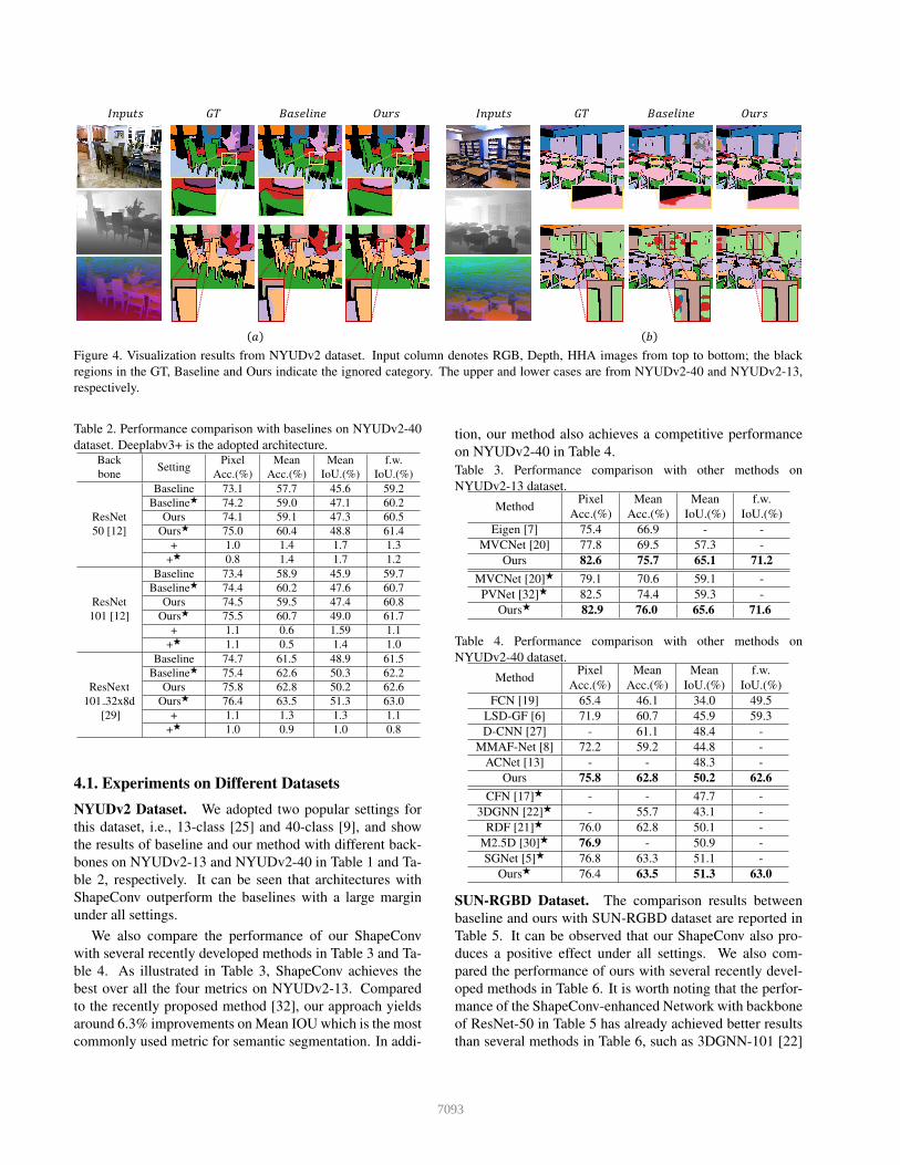
4.3. VisualizationFigure 4 illustrates the qualitative results on NYUDv2-

13 and -40, more results can be found in the Supp. Asshown in this figure, the depth information, especially thedetailed one, can be well utilized by ShapeConv to extractthe object features. For instance, the chair and table re-gions in the top example of Figure 4(a) are with graduallychanged colors, making it hard to predict accurate segmen-tation boundaries of the baseline method. The shape fea-tures learned by ShapeConv makes the accurate cut follow-ing the geometric hints compare with the conventional con-volutional layer. For other two cases, i.e., the chair in thebottom example of Figure 4(a) and the desk in the top exam-ple of Figure 4(b), the ShapeConv can also significantly im-prove the segmentation results in edge areas compared with

7094

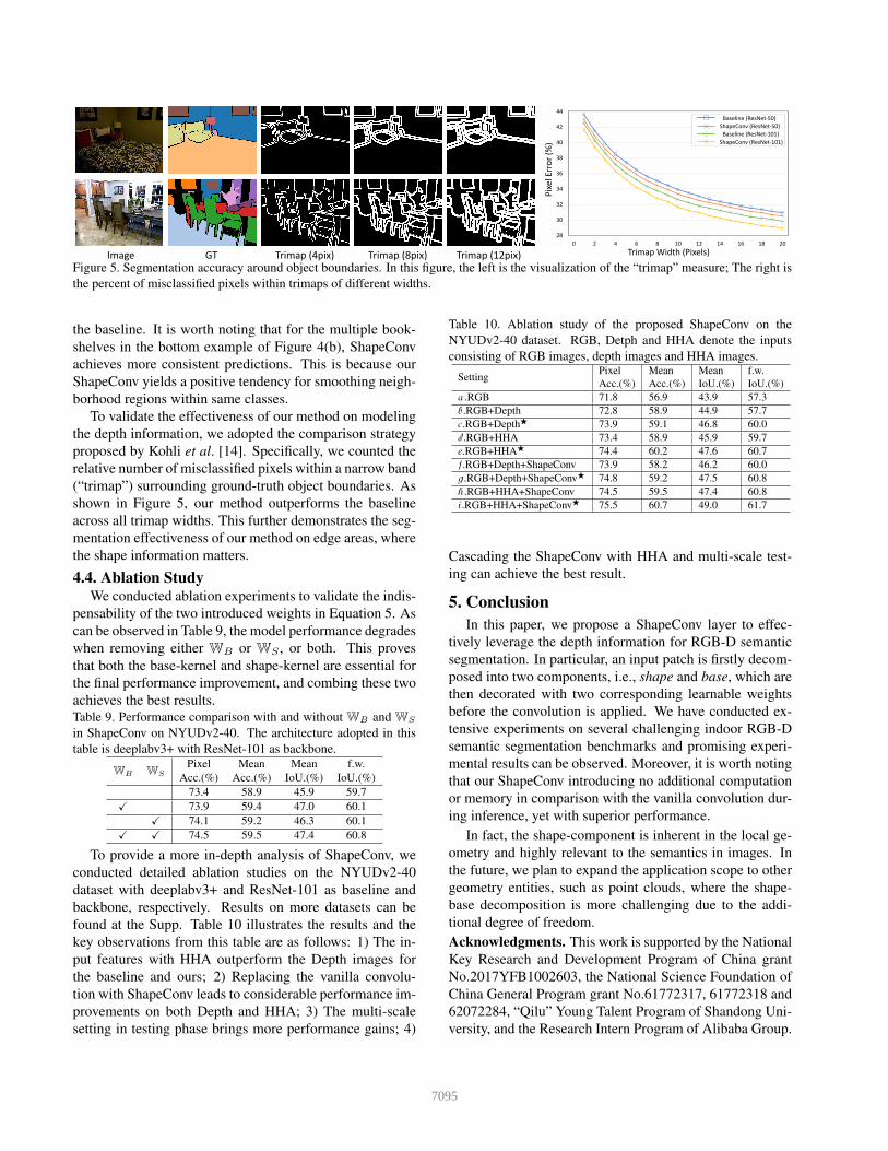
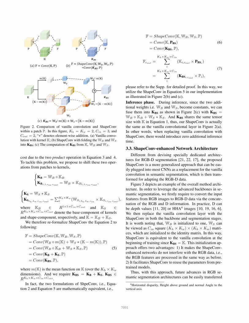
Image GT Trimap (4pix) Trimap (8pix) Trimap (12pix)

Pixe

l Err

or (%

)

Trimap Width (Pixels)

28

30

32

34

36

38

40

42

44

0 2 4 6 8 10 12 14 16 18 20

Baseline (ResNet-50)ShapeConv (ResNet-50)

Baseline (ResNet-101)ShapeConv (ResNet-101)

Figure 5. Segmentation accuracy around object boundaries. In this figure, the left is the visualization of the “trimap” measure; The right isthe percent of misclassified pixels within trimaps of different widths.

the baseline. It is worth noting that for the multiple book-shelves in the bottom example of Figure 4(b), ShapeConvachieves more consistent predictions. This is because ourShapeConv yields a positive tendency for smoothing neigh-borhood regions within same classes.

To validate the effectiveness of our method on modelingthe depth information, we adopted the comparison strategyproposed by Kohli et al. [14]. Specifically, we counted therelative number of misclassified pixels within a narrow band(“trimap”) surrounding ground-truth object boundaries. Asshown in Figure 5, our method outperforms the baselineacross all trimap widths. This further demonstrates the seg-mentation effectiveness of our method on edge areas, wherethe shape information matters.

4.4. Ablation StudyWe conducted ablation experiments to validate the indis-

pensability of the two introduced weights in Equation 5. Ascan be observed in Table 9, the model performance degradeswhen removing either WB or WS , or both. This provesthat both the base-kernel and shape-kernel are essential forthe final performance improvement, and combing these twoachieves the best results.Table 9. Performance comparison with and without WB and WS

in ShapeConv on NYUDv2-40. The architecture adopted in thistable is deeplabv3+ with ResNet-101 as backbone.

WB WSPixel Mean Mean f.w.

Acc.(%) Acc.(%) IoU.(%) IoU.(%)73.4 58.9 45.9 59.7

X 73.9 59.4 47.0 60.1X 74.1 59.2 46.3 60.1

X X 74.5 59.5 47.4 60.8

To provide a more in-depth analysis of ShapeConv, weconducted detailed ablation studies on the NYUDv2-40dataset with deeplabv3+ and ResNet-101 as baseline andbackbone, respectively. Results on more datasets can befound at the Supp. Table 10 illustrates the results and thekey observations from this table are as follows: 1) The in-put features with HHA outperform the Depth images forthe baseline and ours; 2) Replacing the vanilla convolu-tion with ShapeConv leads to considerable performance im-provements on both Depth and HHA; 3) The multi-scalesetting in testing phase brings more performance gains; 4)

Table 10. Ablation study of the proposed ShapeConv on theNYUDv2-40 dataset. RGB, Detph and HHA denote the inputsconsisting of RGB images, depth images and HHA images.

Setting Pixel Mean Mean f.w.Acc.(%) Acc.(%) IoU.(%) IoU.(%)

a.RGB 71.8 56.9 43.9 57.3b.RGB+Depth 72.8 58.9 44.9 57.7c.RGB+DepthF 73.9 59.1 46.8 60.0d.RGB+HHA 73.4 58.9 45.9 59.7e.RGB+HHAF 74.4 60.2 47.6 60.7f.RGB+Depth+ShapeConv 73.9 58.2 46.2 60.0g.RGB+Depth+ShapeConvF 74.8 59.2 47.5 60.8h.RGB+HHA+ShapeConv 74.5 59.5 47.4 60.8i.RGB+HHA+ShapeConvF 75.5 60.7 49.0 61.7

Cascading the ShapeConv with HHA and multi-scale test-ing can achieve the best result.

5. ConclusionIn this paper, we propose a ShapeConv layer to effec-

tively leverage the depth information for RGB-D semanticsegmentation. In particular, an input patch is firstly decom-posed into two components, i.e., shape and base, which arethen decorated with two corresponding learnable weightsbefore the convolution is applied. We have conducted ex-tensive experiments on several challenging indoor RGB-Dsemantic segmentation benchmarks and promising experi-mental results can be observed. Moreover, it is worth notingthat our ShapeConv introducing no additional computationor memory in comparison with the vanilla convolution dur-ing inference, yet with superior performance.

In fact, the shape-component is inherent in the local ge-ometry and highly relevant to the semantics in images. Inthe future, we plan to expand the application scope to othergeometry entities, such as point clouds, where the shape-base decomposition is more challenging due to the addi-tional degree of freedom.Acknowledgments. This work is supported by the NationalKey Research and Development Program of China grantNo.2017YFB1002603, the National Science Foundation ofChina General Program grant No.61772317, 61772318 and62072284, “Qilu” Young Talent Program of Shandong Uni-versity, and the Research Intern Program of Alibaba Group.

7095

References[1] Iro Armeni, Sasha Sax, Amir R Zamir, and Silvio Savarese.

Joint 2d-3d-semantic data for indoor scene understanding.arXiv preprint arXiv:1702.01105, 2017.

[2] Liang-Chieh Chen, George Papandreou, Iasonas Kokkinos,Kevin Murphy, and Alan L Yuille. Deeplab: Semantic imagesegmentation with deep convolutional nets, atrous convolu-tion, and fully connected crfs. IEEE transactions on patternanalysis and machine intelligence, 40(4):834–848, 2017.

[3] Liang-Chieh Chen, George Papandreou, Florian Schroff, andHartwig Adam. Rethinking atrous convolution for seman-tic image segmentation. arXiv preprint arXiv:1706.05587,2017.

[4] Liang-Chieh Chen, Yukun Zhu, George Papandreou, FlorianSchroff, and Hartwig Adam. Encoder-decoder with atrousseparable convolution for semantic image segmentation. InProceedings of the European Conference on Computer Vi-sion, pages 801–818, 2018.

[5] Lin-Zhuo Chen, Zheng Lin, Ziqin Wang, Yong-Liang Yang,and Ming-Ming Cheng. Spatial information guided convolu-tion for real-time rgbd semantic segmentation. IEEE Trans-actions on Image Processing, 30:2313–2324, 2021.

[6] Yanhua Cheng, Rui Cai, Zhiwei Li, Xin Zhao, and KaiqiHuang. Locality-sensitive deconvolution networks withgated fusion for rgb-d indoor semantic segmentation. In Pro-ceedings of the IEEE Conference on Computer Vision andPattern Recognition, pages 3029–3037, 2017.

[7] David Eigen and Rob Fergus. Predicting depth, surface nor-mals and semantic labels with a common multi-scale con-volutional architecture. In Proceedings of the IEEE Inter-national Conference on Computer Vision, pages 2650–2658,2015.

[8] Fahimeh Fooladgar and Shohreh Kasaei. Multi-modalattention-based fusion model for semantic segmentation ofrgb-depth images. arXiv preprint arXiv:1912.11691, 2019.

[9] Saurabh Gupta, Pablo Arbelaez, and Jitendra Malik. Per-ceptual organization and recognition of indoor scenes fromrgb-d images. In Proceedings of the IEEE Conference onComputer Vision and Pattern Recognition, pages 564–571,2013.

[10] Saurabh Gupta, Ross Girshick, Pablo Arbelaez, and JitendraMalik. Learning rich features from rgb-d images for objectdetection and segmentation. In Proceedings of the EuropeanConference on Computer Vision, pages 345–360. Springer,2014.

[11] Caner Hazirbas, Lingni Ma, Csaba Domokos, and DanielCremers. Fusenet: Incorporating depth into semantic seg-mentation via fusion-based cnn architecture. In Asian Con-ference on Computer Vision, pages 213–228. Springer, 2016.

[12] Kaiming He, Xiangyu Zhang, Shaoqing Ren, and Jian Sun.Deep residual learning for image recognition. In Proceed-ings of the IEEE Conference on Computer Vision and PatternRecognition, pages 770–778, 2016.

[13] Xinxin Hu, Kailun Yang, Lei Fei, and Kaiwei Wang. Acnet:Attention based network to exploit complementary featuresfor rgbd semantic segmentation. In 2019 IEEE International

Conference on Image Processing (ICIP), pages 1440–1444.IEEE, 2019.

[14] Pushmeet Kohli, Philip HS Torr, et al. Robust higher or-der potentials for enforcing label consistency. InternationalJournal of Computer Vision, 82(3):302–324, 2009.

[15] Siqi Li, Changqing Zou, Yipeng Li, Xibin Zhao, and YueGao. Attention-based multi-modal fusion network for se-mantic scene completion. In Proceedings of the AAAI Con-ference on Artificial Intelligence, volume 34, pages 11402–11409, 2020.

[16] Zhen Li, Yukang Gan, Xiaodan Liang, Yizhou Yu, HuiCheng, and Liang Lin. Lstm-cf: Unifying context modelingand fusion with lstms for rgb-d scene labeling. In Proceed-ings of the European Conference on Computer Vision, pages541–557. Springer, 2016.

[17] Di Lin, Guangyong Chen, Daniel Cohen-Or, Pheng-AnnHeng, and Hui Huang. Cascaded feature network for se-mantic segmentation of rgb-d images. In Proceedings of theIEEE International Conference on Computer Vision, pages1311–1319, 2017.

[18] Tsung-Yi Lin, Piotr Dollar, Ross Girshick, Kaiming He,Bharath Hariharan, and Serge Belongie. Feature pyramidnetworks for object detection. In Proceedings of the IEEEConference on Computer Vision and Pattern Recognition,pages 2117–2125, 2017.

[19] Jonathan Long, Evan Shelhamer, and Trevor Darrell. Fullyconvolutional networks for semantic segmentation. In Pro-ceedings of the IEEE Conference on Computer Vision andPattern Recognition, pages 3431–3440, 2015.

[20] Lingni Ma, Jorg Stuckler, Christian Kerl, and Daniel Cre-mers. Multi-view deep learning for consistent semantic map-ping with rgb-d cameras. In 2017 IEEE/RSJ InternationalConference on Intelligent Robots and Systems (IROS), pages598–605. IEEE, 2017.

[21] Seong-Jin Park, Ki-Sang Hong, and Seungyong Lee. Rdfnet:Rgb-d multi-level residual feature fusion for indoor seman-tic segmentation. In Proceedings of the IEEE InternationalConference on Computer Vision, pages 4980–4989, 2017.

[22] Xiaojuan Qi, Renjie Liao, Jiaya Jia, Sanja Fidler, and RaquelUrtasun. 3d graph neural networks for rgbd semantic seg-mentation. In Proceedings of the IEEE International Con-ference on Computer Vision, pages 5199–5208, 2017.

[23] Olaf Ronneberger, Philipp Fischer, and Thomas Brox. U-net: Convolutional networks for biomedical image segmen-tation. In International Conference on Medical Image Com-puting and Computer-assisted Intervention, pages 234–241.Springer, 2015.

[24] Olga Russakovsky, Jia Deng, Hao Su, Jonathan Krause, San-jeev Satheesh, Sean Ma, Zhiheng Huang, Andrej Karpathy,Aditya Khosla, Michael Bernstein, et al. ImageNet largescale visual recognition challenge. International Journal ofComputer Vision, 115(3):211–252, 2015.

[25] Nathan Silberman, Derek Hoiem, Pushmeet Kohli, and RobFergus. Indoor segmentation and support inference fromrgbd images. In Proceedings of the European Conferenceon Computer Vision, pages 746–760. Springer, 2012.

[26] Shuran Song, Samuel P Lichtenberg, and Jianxiong Xiao.Sun rgb-d: A rgb-d scene understanding benchmark suite.

7096

In Proceedings of the IEEE Conference on Computer Visionand Pattern Recognition, pages 567–576, 2015.

[27] Weiyue Wang and Ulrich Neumann. Depth-aware cnn forrgb-d segmentation. In Proceedings of the European Confer-ence on Computer Vision, pages 135–150, 2018.

[28] Yikai Wang, Wenbing Huang, Fuchun Sun, Tingyang Xu, YuRong, and Junzhou Huang. Deep multimodal fusion by chan-nel exchanging. Advances in Neural Information ProcessingSystems, 33, 2020.

[29] Saining Xie, Ross Girshick, Piotr Dollar, Zhuowen Tu, andKaiming He. Aggregated residual transformations for deepneural networks. In Proceedings of the IEEE Conferenceon Computer Vision and Pattern Recognition, pages 1492–1500, 2017.

[30] Yajie Xing, Jingbo Wang, and Gang Zeng. Malleable 2.5 dconvolution: Learning receptive fields along the depth-axisfor rgb-d scene parsing. arXiv preprint arXiv:2007.09365,2020.

[31] Zhengyou Zhang. Microsoft kinect sensor and its effect.IEEE multimedia, 19(2):4–10, 2012.

[32] Cheng Zhao, Li Sun, Pulak Purkait, Tom Duckett, and Rus-tam Stolkin. Dense rgb-d semantic mapping with pixel-voxelneural network. Sensors, 18(9):3099, 2018.

[33] Hengshuang Zhao, Jianping Shi, Xiaojuan Qi, XiaogangWang, and Jiaya Jia. Pyramid scene parsing network. In Pro-ceedings of the IEEE Conference on Computer Vision andPattern Recognition, pages 2881–2890, 2017.

7097

shapeconv: shape-aware convolutional layer for indoor

Documents