hedge backpropagation in convolutional neural networks

University of Groningen,

the Netherlands

Master’s ThesisArtificial Intelligence

Hedge Backpropagation inConvolutional Neural Networks

Floris van Beerss2197367

Internal Supervisor:Dr. M. A. Wiering (Artificial Intelligence, University of Groningen)

[Dr. H. Jaeger (Artificial Intelligence, University of Groningen)]External Supervisors:

Dr. L. Hogeweg (Machine Learning Researcher, Intel Corporation)

November 24, 2021

Abstract

In the field of object recognition much is gained by the use of convolutional neuralnetworks (CNNs). Research into deeper networks has revealed untold successes,as well as unforeseen issues. Ensembles of deep CNNs are being used to furtherimprove performance, while the issues with vanishing gradients have been tackledby the use of deep supervision. In this work a novel architecture is proposedwhich combines these techniques. Using ResNet34 and DenseNet121 as basevariants, a Multiple Heads (MH) adaptation attempts to improve performanceand solve issues. Further work on the weights (α) in the MH variant leads to useof the Hedge Back Propagation (HBP) algorithm in the HBP and Thaw modelvariants. Experiments on CIFAR10 and the Naturalis Papilionidae datasets showthe use of MH variants improves over base networks in one of the experimentalsettings. The application of HBP does not further improve the performance ofthe MH variant, but leads to interesting observations resulting in a multitude ofdirections for future work.

I

Acknowledgement

For being my biggest supporter during my studies, my internship and mythesis, I want to thank my wife, Nury, from the bottom of my heart.

It is with great sadness that I say goodbye to Marco Wiering, who’s guidancehelped start, shape and grow this project. He has been a mentor to me throughoutthis and other projects, and my studies as a whole. His sudden passing cameas a shock and has prohibited us from seeing the project through together. Hiscontributions to our shared projects, and to the science community as a whole,will not be forgotten.

I am indebted to Herbert Jaeger, who stepped up on very short notice tofinish the project with me. I am thankful for his wise words on the project, aswell as Marco’s passing.

To be able to work on my research during an internship at Intel Corporation,to meet many experienced, driven and wonderful people, I am grateful. I wantto explicitly state my appreciation for all the time, energy and ideas LaurensHogeweg invested in me as my project supervisor.

For all the support during my years of study, personal, financial and educa-tional, I thank my loving parents.

II

Contents

1 Introduction 11.1 Research Questions . . . . . . . . . . . . . . . . . . . . . . . . . . 21.2 Thesis Structure . . . . . . . . . . . . . . . . . . . . . . . . . . . 3

2 Theoretical background 42.1 Deep Learning . . . . . . . . . . . . . . . . . . . . . . . . . . . . 4

2.1.1 Neural Networks . . . . . . . . . . . . . . . . . . . . . . . 42.1.2 Convolutional Layers . . . . . . . . . . . . . . . . . . . . . 52.1.3 Vanishing Gradient Problem and Solutions . . . . . . . . 5

2.2 Deep Supervision . . . . . . . . . . . . . . . . . . . . . . . . . . . 62.3 Ensemble Learning . . . . . . . . . . . . . . . . . . . . . . . . . . 7

3 Methodology 83.1 Hedge Algorithm . . . . . . . . . . . . . . . . . . . . . . . . . . . 8

3.1.1 Hedge Backpropagation . . . . . . . . . . . . . . . . . . . 93.2 Models . . . . . . . . . . . . . . . . . . . . . . . . . . . . . . . . . 11

3.2.1 ResNet34 . . . . . . . . . . . . . . . . . . . . . . . . . . . 113.2.2 DenseNet121 . . . . . . . . . . . . . . . . . . . . . . . . . 123.2.3 Multiple Heads Variants . . . . . . . . . . . . . . . . . . . 133.2.4 HBP Variants . . . . . . . . . . . . . . . . . . . . . . . . . 143.2.5 Thawing HBP Variants . . . . . . . . . . . . . . . . . . . 14

3.3 Data . . . . . . . . . . . . . . . . . . . . . . . . . . . . . . . . . . 173.3.1 CIFAR10 . . . . . . . . . . . . . . . . . . . . . . . . . . . 173.3.2 Naturalis Papilionidae . . . . . . . . . . . . . . . . . . . . 17

4 Experimental Setup 194.1 Preprocessing . . . . . . . . . . . . . . . . . . . . . . . . . . . . . 19

4.1.1 Data Augmentation . . . . . . . . . . . . . . . . . . . . . 194.2 Hyper Parameter Optimization . . . . . . . . . . . . . . . . . . . 204.3 Experimental settings . . . . . . . . . . . . . . . . . . . . . . . . 22

4.3.1 Early Stopping . . . . . . . . . . . . . . . . . . . . . . . . 224.4 Specifications . . . . . . . . . . . . . . . . . . . . . . . . . . . . . 23

4.4.1 Hardware . . . . . . . . . . . . . . . . . . . . . . . . . . . 234.4.2 Software . . . . . . . . . . . . . . . . . . . . . . . . . . . . 23

III

5 Results 245.1 Does a model with multiple heads perform better than the base

model? . . . . . . . . . . . . . . . . . . . . . . . . . . . . . . . . . 265.1.1 Why does the difference in performance on CIFAR10 not

translate to Papilionidae, both with and without transferlearning? . . . . . . . . . . . . . . . . . . . . . . . . . . . 26

5.2 Do the additional heads increase performance when active duringinference? . . . . . . . . . . . . . . . . . . . . . . . . . . . . . . . 30

5.3 Does the hedge backpropagation (HBP) algorithm successfullyoptimize weights between output layers of a model with multipleheads? . . . . . . . . . . . . . . . . . . . . . . . . . . . . . . . . . 34

5.4 Does freezing the weights assigned to classifiers in the model atthe start of training influence the performance of the model? . . 39

5.5 Do the behaviours of these models change when using differingamounts of data? . . . . . . . . . . . . . . . . . . . . . . . . . . . 43

6 Discussion 456.1 Research Questions . . . . . . . . . . . . . . . . . . . . . . . . . . 456.2 Conclusions . . . . . . . . . . . . . . . . . . . . . . . . . . . . . . 476.3 Recommendations for Future Research . . . . . . . . . . . . . . . 48

7 Appendix A - Full Results 54

IV

List of Figures

3.1 Abstract model structure for all models with multiple classifiers(MH-variants, HBP-variants, Thaw-variants). Data flow repre-sents loss by individual classifiers, which is used to update separateparts of the network. . . . . . . . . . . . . . . . . . . . . . . . . . 15

3.2 Abstract model structure for all models with multiple classifiers(MH-variants, HBP-variants, Thaw-variants). Data flow repre-sents shows combined final output, used to determine accuracy ofthe model. . . . . . . . . . . . . . . . . . . . . . . . . . . . . . . . 16

3.3 Two examples from the Papilionidae dataset . . . . . . . . . . . . 18

5.1 Accuracy and loss of ResNet34 and MHResNet34 on CIFAR10 . 275.2 Accuracy and loss of DenseNet121 and MHDensenet121 on CIFAR10 285.3 Accuracy and loss of ResNet34 and MHResNet34 on Papilionidae,

untrained . . . . . . . . . . . . . . . . . . . . . . . . . . . . . . . 285.4 Accuracy and loss of DenseNet121 and MHDenseNet121 on Pa-

pilionidae, untrained . . . . . . . . . . . . . . . . . . . . . . . . . 295.5 Accuracy and loss of ResNet34 and MHResNet34 on Papilionidae,

pretrained . . . . . . . . . . . . . . . . . . . . . . . . . . . . . . . 295.6 Accuracy and loss of DenseNet121 and MHDenseNet121 on Pa-

pilionidae, pretrained . . . . . . . . . . . . . . . . . . . . . . . . . 305.7 Results for MHResNet34 for individual classifiers on CIFAR10 . 315.8 Results MHDenseNet121 for individual classifiers on CIFAR10 . 325.9 Results for MHResNet34 for individual classifiers on Papilionidae,

untrained . . . . . . . . . . . . . . . . . . . . . . . . . . . . . . . 325.10 Results MHDenseNet121 for individual classifiers on Papilionidae,

untrained, . . . . . . . . . . . . . . . . . . . . . . . . . . . . . . . 335.11 Results for MHResNet34 for individual classifiers on Papilionidae,

pretrained . . . . . . . . . . . . . . . . . . . . . . . . . . . . . . . 335.12 Results MHDenseNet121 for individual classifiers on Papilionidae,

pretrained . . . . . . . . . . . . . . . . . . . . . . . . . . . . . . . 345.13 Results for HBPResNet34 for individual classifiers on CIFAR10 . 365.14 Results HBPDenseNet121 for individual classifiers on CIFAR10 . 365.15 Results for HBPResNet34 for individual classifiers on Papilionidae,

untrained . . . . . . . . . . . . . . . . . . . . . . . . . . . . . . . 37

V

5.16 Results HBPDenseNet121 for individual classifiers on Papilionidae,untrained . . . . . . . . . . . . . . . . . . . . . . . . . . . . . . . 37

5.17 Results for HBPResNet34 for individual classifiers on Papilionidae,pretrained . . . . . . . . . . . . . . . . . . . . . . . . . . . . . . . 38

5.18 Results HBPDenseNet121 for individual classifiers on Papilionidae,pretrained . . . . . . . . . . . . . . . . . . . . . . . . . . . . . . . 38

5.19 Results for ThawResNet34 for individual classifiers on CIFAR10 405.20 Results ThawDenseNet121 for individual classifiers on CIFAR10 405.21 Results for ThawResNet34 for individual classifiers on Papilion-

idae, untrained . . . . . . . . . . . . . . . . . . . . . . . . . . . . 415.22 Results ThawDenseNet121 for individual classifiers on Papilion-

idae, untrained . . . . . . . . . . . . . . . . . . . . . . . . . . . . 415.23 Results for ThawResNet34 for individual classifiers on Papilion-

idae, pretrained . . . . . . . . . . . . . . . . . . . . . . . . . . . . 425.24 Results ThawDenseNet121 for individual classifiers on Papilion-

idae, pretrained . . . . . . . . . . . . . . . . . . . . . . . . . . . . 425.25 Mean results for all models on all folds for CIFAR10, plotted over

the amount of data used. . . . . . . . . . . . . . . . . . . . . . . 435.26 Mean results for all models on all folds for Papilionidae, untrained,

plotted over the amount of data used. . . . . . . . . . . . . . . . 445.27 Mean results for all models on all folds for Papilionidae, pretrained,

plotted over the amount of data used. . . . . . . . . . . . . . . . 44

VI

List of Tables

3.1 Number of model parameters . . . . . . . . . . . . . . . . . . . . 14

4.1 Hyper parameter optimization on s for HBPResNet34 . . . . . . 204.2 Hyper parameter optimization on s for HBPDenseNet121 . . . . 214.3 Thawing behaviour in epochs depending on θ and γ values . . . . 214.4 Hyper parameter optimization on θ/γ for ThawResNet34 . . . . 214.5 Hyper parameter optimization on θ/γ for ThawDenseNet34 . . . 22

5.1 Results on CIFAR10 for all models, with different numbers oftraining samples . . . . . . . . . . . . . . . . . . . . . . . . . . . 25

5.2 Results on Papilionidae for all models without transfer learning,with different numbers of training samples . . . . . . . . . . . . . 25

5.3 Results on Papilionidae for all models with transfer learning, withdifferent numbers of training samples . . . . . . . . . . . . . . . . 25

5.4 Comparison of ResNet34 and MHResNet34 by pairwise t-test . . 265.5 Comparison of DenseNet121 and MHDenseNet121 by pairwise t-test 275.6 Comparison of MHResNet34 and HBPResNet34 by pairwise t-test 355.7 Comparison of MHDebseNet121 and HBPDenseNet121 by pair-

wise t-test . . . . . . . . . . . . . . . . . . . . . . . . . . . . . . . 355.8 Comparison of MHResNet34 and HBPResNet34 with ThawRes-

Net34 by pairwise t-test . . . . . . . . . . . . . . . . . . . . . . . 395.9 Comparison of MHDenseNet121 and HBPDenseNet121 with Thaw-

DenseNet121 by pairwise t-test . . . . . . . . . . . . . . . . . . . 43

7.1 CIFAR10 with 5% of training data . . . . . . . . . . . . . . . . . 547.2 CIFAR10 with 10% of training data . . . . . . . . . . . . . . . . 557.3 CIFAR10 with 20% of training data . . . . . . . . . . . . . . . . 557.4 CIFAR10 with 50% of training data . . . . . . . . . . . . . . . . 557.5 CIFAR10 with 100% of training data . . . . . . . . . . . . . . . . 567.6 Papilionidae, untrained, with 5% of training data . . . . . . . . . 567.7 Papilionidae, untrained, with 10% of training data . . . . . . . . 567.8 Papilionidae, untrained, with 20% of training data . . . . . . . . 577.9 Papilionidae, untrained, with 50% of training data . . . . . . . . 577.10 Papilionidae, untrained, with 100% of training data . . . . . . . . 577.11 Papilionidae, pretrained, with 5% of training data . . . . . . . . 58

VII

7.12 Papilionidae, pretrained, with 10% of training data . . . . . . . . 587.13 Papilionidae, pretrained, with 20% of training data . . . . . . . . 587.14 Papilionidae, pretrained, with 50% of training data . . . . . . . . 597.15 Papilionidae, pretrained, with 100% of training data . . . . . . . 59

VIII

Chapter 1

Introduction

Image classification is a task that has seen numerous solutions, with differing,but increasing, amounts of success. The number of applications is equally large,and growing. Due to all this interest in image classification, improvements havebeen made at a rapid pace. The task can be defined as using a system of rulesto automatically label an image with the correct class label in a specific setof images. From this definition it can be seen that attempts to solve imageclassification can be performed simply by hand, by flow-chart, by more complexmathematical analysis, and ultimately by automated pattern recognition.

The biggest breakthrough in image classification in the last decades has beenwith the introduction of the convolutional neural network (CNN) [Lecun et al., 1998]and its first show of force [Krizhevsky et al., 2012]. CNNs have been the go-tosystem of rules applied to image classification. While this narrows the range ofsolutions to the task, these models have shown to be very effective. Additionally,this choice of solution in no way narrows the immensely broad applications forthis task. These applications include object classification by cameras on anautonomous robot for scene understanding [Ye et al., 2017], medical imagingto determine the health of a tissue [Gertych et al., 2019], fine-grained animalclassification to aid in determining biodiversity [Marre et al., 2020], and so on.

With the success of AlexNet [Krizhevsky et al., 2012] came the increasedattention by the scientific community that led to numerous improvements tothe first functional CNN. While many of these improvements were developedto incrementally increase the effectiveness of a model, some improvements weremore drastic, both in structural impact as well as necessity. Most notablehas been the effort to train ever deeper CNNs which introduced the vanishinggradient problem.

The vanishing gradient problem occurs when CNNs are made consistentlydeeper, meaning they consist of more layers. In general terms, the problem occurswhen models are so deep that any information used to train the network is lostduring backpropagation. Due to this, the earlier layers of a network do not receiveany information from which they can learn. The solution to this problem hasseen many forms, from mathematical adjustments such as a different activation

1

function [Xu et al., 2015], to structural solutions such as adjusting the con-nections between shallow and deep layers [He et al., 2016, Huang et al., 2017b].The most impactful structural change to accommodate for this problem hasbeen the use of auxiliary heads [Szegedy et al., 2015], a technique more generallyknown as deep supervision [Wang et al., 2015, Lee et al., 2015]. The additionof auxiliary heads allows shallow layers to be trained more directly, allowingmore information to be learned by these layers. It has shown to be effective intraining deep neural networks that would otherwise be untrainable.

A second, large, structural change used to improve results beyond incrementaladvances has been ensemble learning. This technique uses a group, or ensemble,of effective models and combines their output to produce its final prediction[Dietterich, 2000]. Using multiple models trained on similar data can produce anensemble where each individual model’s bias towards local minima or specific over-represented classes is negated by the combined output of the group. However, anensemble in the naive sense requires training multiple models which, obviously,requires more time and computing power. To reduce these negative effectsof using an ensemble, several methods try to reuse parts of the model in theensemble [Minetto et al., 2019, Huang et al., 2017a].

In this work, several novel model structures and a corresponding training algo-rithm are introduced, adapted from work in online deep learning [Sahoo et al., 2018].These novel structures use the auxiliary heads as seen in deep supervision[Szegedy et al., 2015, Wang et al., 2015, Lee et al., 2015]. In contrast to thesetechniques, the multiple heads (MH) are kept active during inference, resultingin a model that is an ensemble of itself and shallower versions of itself. Inaddition to this new model structure, the technique of hedge backpropagation(HBP) [Sahoo et al., 2018] is adapted to convolutional neural networks. Thistechnique then allows the model to learn the weight of each head during training,resulting in two additional model structures. The models using MH withoutHBP are named MHResNet34 and MHDenseNet121, based on ResNet34 andDenseNet121 respectively. The models using HBP are named HBPResNet34 andHBPDenseNet121. Finally, a hybrid implementation of MH and HBP results inThawResNet34 and ThawDenseNet121.

1.1 Research Questions

The development of the model structures described in Chapter 1 and their effec-tiveness compared to the base models is the core of this work. This comparisoncan be made in several steps, each represented by a separate research question:

1. Does a model with auxiliary heads perform better than the base model?

2. Do the auxiliary heads increase performance when active during inference,in contrast to only using auxiliary heads during training?

3. Does the hedge backpropagation (HBP) algorithm successfully optimizeweights between output layers of a model with multiple heads?

2

4. Does freezing the weights assigned to classifiers in the model at the startof training influence the performance of the model? Does this significantlydiffer from the MH or HBP models?

5. Do the behaviours of these models change when using differing amounts ofdata?

1.2 Thesis Structure

This section has given a very brief summary of the goals of this work. InChapter 2, each topic mentioned in this summary will be more fully put intoits scientific context. Chapter 3 will then introduce the new additions of thiswork formally, together with the data used. To measure the effectiveness ofthese methods, a multitude of experiments was set up, described in Chapter 4.The experimental results are shown in Chapter 5, together with the statisticalanalysis. Finally, Chapter 6 will answer the research questions, along with otherrelevant conclusions, before listing suggestions for future research.

3

Chapter 2

Theoretical background

2.1 Deep Learning

The origins of Deep Learning (DL) can be traced back all the way to the Rosen-blatt perceptron [Rosenblatt, 1958]. This mathematical operation is nothingmore than a weighted sum of inputs, producing an output of 1 if this sumcrosses a threshold and 0 otherwise. This operation, in addition to a function toupdate the weights, is the basis of the artificial neuron. Several adaptations andextensions made to the perceptron have produced the earliest neural networkmodels called Multi-Layer Perceptrons (MLPs). These adaptations are stackingthe perceptrons in layers, using a more complex update algorithm, and usingnon-linear activation of the individual neurons.

2.1.1 Neural Networks

The effectiveness of neural networks lies in its power to update weights ofmultiple layers of neurons with non-linear activations by determining eachneurons contribution to the output. The usefulness of these models is in the useof non-linear activations. By stacking non-linear activations, a neural networkas simple as an MLP can be used as an universal function approximator.

To train a neural network for a specific task an iterative procedure is appliedof alternating between forward and backward passes. The forward passes feedthe network, or model, a set of inputs to which the network then connects anoutput, e.g. a class label. The backward passes calculate the error between theoutput and the desired label and update the weights of each layer according tothis error in a process called backpropagation [Rumelhart et al., 1986]. Finally,the iterative process of updating the weights in the direction that minimizeserror is done by a gradient descent algorithm. The necessity for labeled samplesmakes training a neural network a supervised learning task.

4

Backpropagation

The technique of backpropagation [Rumelhart et al., 1986], which allows net-works with more than a single layer to train the weights connected to non-outputlayers, is a cornerstone of neural networks. The use of chained partial derivativesallows information about the gradient used by gradient descent to flow backwardthrough the model, starting at the output layer. This allows a single errorcalculation in the final layer to affect all weights in the model.

2.1.2 Convolutional Layers

A big leap forward in using neural networks for image processing has been madethrough the development of Convolutional Neural Networks [Krizhevsky et al., 2012,Simonyan and Zisserman, 2015]. These networks, as the name suggests, use con-volutions, built into seperate layers called convolutional layers. These layers usefeature maps to detect features in localized areas of their input, giving themthe possibility of detecting spatial relations between input values (pixels). Thisallows much more relevant information to be extracted from images. Additionally,applying filters, or kernels, to these localized areas allows for weight sharing,since a single kernel has identical weights regardless of which patch of the inputit is currently applying the filter to. These two factors allow for more informationretention with less parameters, greatly increasing performance on image-baseddata, where spatial relations are relevant.

Multiple stacked convolutional layers can turn lower level features, such aslines and shapes, into higher level features such as facial features, windows in abuilding, or legs of an animal. Together with intermittent pooling layers, thesefeatures are effectively combined to correctly identify an entire object by addingnumerous features together into a single output. The final output of features isthen used by a conventional (set of) layer(s) to correctly label the input.

2.1.3 Vanishing Gradient Problem and Solutions

Initial attempts to improve CNNs frequently led to increases in the number of con-volutional layers, with 2 layer in LeNet [Lecun et al., 1998], 5 layers in AlexNet[Krizhevsky et al., 2012], and 16 in VGG19 [Simonyan and Zisserman, 2015].Attempts to go larger ran into issues with backpropagation. This issue was coinedthe vanishing gradient problem [Hochreiter, 1991, Kolen and Kremer, 2001].

The vanishing gradient problem describes the inability for significantly deepneural networks to learn any significant patterns in their early layers. This iscaused by the process of chaining partial derivatives. If we assume the activationfunction of each layer has gradient < 0, 1 >, such as with the sigmoid activation(Equation 2.1) or hyperbolic tangent activation (Equation 2.2), the gradient giof layer i will be gi =< 0, 1 >i due to the chained nature of backpropagation.The more these gradients approach 0, the quicker the value for gi approaches0. A layer with gradient 0 will not update its weights and therefore not learnanything. If this happens later in the learning process, the route to an optimal

5

solution is stifled. However, if this happens much earlier, the early layers will beuntrained and will be, at best, useless, and might even be detrimental by actingas a filter applying noise to the input.

σ(x) =1

1 + ex(2.1)

tanh(x) =ex − e−x

ex + e−x(2.2)

An initial, and intuitive, response to this problem is to replace the activationfunction with one that does not exhibit this behaviour. The current standardfor this is the rectified linear unit (ReLU) activation. This activation, describedby Equation 2.3, provides a gradient that is either 1 or 0, removing the situationof arbitrarily small gradients being multiplied and vanishing.

ReLU(x) = max(0, x) (2.3)

Another solution is to increase the connection between the output layerand early convolutional layers in the network. These connections are generallycalled skip connections, as they skip one or more layers of the model. Theseskip connections ensure information from earlier layers reaches the final outputand thus impacts the gradient for these early layers, negating the devastatingeffect of the vanishing gradient problem. Skip connections come in two variants:additive connections, leading to ResNet variants [He et al., 2016], where theinput of a block of layers is added to the output of that block, and concatenatedconnections, resulting in DenseNet variants [Huang et al., 2017b], where thefeatures of previous blocks are added to the output of the current block as acombined input to the next block. Both these variants and their workings arefurther explained in Section 3.2.

Regardless of technique, the goal of solving the vanishing gradient problem isto allow the training of deeper neural networks. Another technique developed forthis goal structurally changes the architecture of the model by adding additionaloutput layers. This area of research is known as deep supervision.

2.2 Deep Supervision

Deep supervision is the technique of adding auxiliary output branches, or aux-iliary heads, to the model at halfway points to give earlier layers more directfeedback [Wang et al., 2015, Lee et al., 2015]. Extending the concept of super-vised learning, this allows the supervisor (i.e. the user with labeled data), toprovide this feedback at multiple depths.

Deep supervision has been used to train state-of-the-art models, such asInception [Szegedy et al., 2015] and Inception v3 [Szegedy et al., 2016]. Thesemodels use auxiliary classifiers at predetermined points during training. Atinference time, when the model is sufficiently trained at every layer, the auxiliaryheads are disconnected, producing a feed forward network. During training,

6

the auxiliary heads provide additional gradient information according to presetweights, which are hyper-parameters to be optimized by the user.

Deep supervision has seen many developments, such as using intermediateconcepts [Li et al., 2019] and knowledge synergy [Sun et al., 2019].

With the wide use of certain popular models such as ResNet50 [He et al., 2016]and Inception V3 [Szegedy et al., 2016], deep supervision has fallen off in usedue to the prevalence of pretrained weights. However, it is also shown that whenmodels are developed specifically for new tasks, and as such no pre-training isavailable, use of deep supervision can greatly improve the training time andperformance of these models [Shen et al., 2020], or might even be the factor thatallows training altogether [Szegedy et al., 2016].

2.3 Ensemble Learning

While new models are continually developed and improve on the state-of-the-art, there is no guarantee that the best performing model overall, in termsof accuracy, performs the best in every possible case of that task. In otherwords, two models of comparable architectures might be specialized in detectingtwo different classes, which performing worse in the class the other model isspecialized in. To use this information as a benefit, ensemble learning has beendeveloped [Dietterich, 2000, Zhou et al., 2002].

While there are many ways to combine the used models into an ensemble,the baseline remains that multiple models need to be trained for the ensem-ble to be effective. Naturally, this puts a heavier burden on computationalresources compared to training a single model. To this end, architectures havebeen developed that reuse some of the weights of the model, to reduce thenecessary resources. This has been done by weight sharing up to a certain depthand fine-tuning only the final layers of the same model in different directions[Minetto et al., 2019]. Alternatively, models have been trained to convergence,while intermediate weights are saved as snapshots. These snapshots are then usedto initialize separate instances of the same model, which can then be combinedinto an ensemble [Huang et al., 2017a]. These architectures show the necesityfor ensemble learning to be more efficient than the naive approach of trainingmany different models individually.

7

Chapter 3

Methodology

While deep supervision and ensemble learning are in itself established develop-ments, this chapter will introduce a novel method, intended to combine strengthsfrom both these concepts.

3.1 Hedge Algorithm

The hedge algorithm [Freund and Schapire, 1997] is an algorithm developed todetermine the proper weights to assign to each output in a system of experts inorder to obtain the best aggregated performance. The algorithm, as shown inpseudo-code in Algorithm 1, can be used for many purposes.

Algorithm 1: Hedge Algorithm Weight (α) Updates

Data: Pair of (data, label) = (x,y)Result: Adapted weights ααi(0) = 1

N where N is number of experts;t = 0;T = number of epochs;for t in range(T) do

for i in range(N) doyi = experti(x);li(t) = f(yi, y);

αi(t+ 1) = αi(t) × βli(t);

end

end

In this algorithm, α is the array of values αi, where i indicates a singleExpert. f(yi, y) denotes the loss function applied to prediction yi and true labely. Finally, β is the discount factor, between 0 and 1, used to determine thereduction in weight αi as a result of the loss produced by expert i. The valuefor β is set in the range 0 < β < 1. A β value of <= 0 would put the weight forthat expert at or below 0, making it irrelevant. In contrast, a β value of >= 1

8

would mean the weight is increasing with a higher loss value, giving the oppositeof the desired effect. In practice, however, the β value is a value close to 1, suchas 0.99, to ensure a gradual change in α.

In any environment with multiple experts with uncertainty to which expertsperforms best, the hedge algorithm can be used to determine expert comparativeeffectiveness. The algorithm has been used, for example, in stock trading[Yutong and Zhao, 2015], and disease classification [Sigcha et al., 2021]. Thealgorithm is specifically designed for such a system of experts to converge on aresult approximating the result of the best expert. It can be proven that thedifference in loss between the total model and the best expert decreases at therate of O

√(lnN)/T , as done so in the work where the Hedge algorithm was

introduced [Freund and Schapire, 1997]. As such, given enough time, the hedgealgorithm will perform equal to a best expert, without needing the knowledge ofwhich expert is best beforehand.

3.1.1 Hedge Backpropagation

An ensemble of neural networks is effectively a system of experts with uncertaintyabout the best performing expert. Multiple methods exist of combining modeloutputs into a single system output, such as averaging or voting, a weightedcombination is the most adaptive method. To determine these weights, thehedge algorithm can be used. Hedging produces an extra weight, or αi for eachmodel i to be used at inference to determine the output of the system. However,this αi can also be used in updating the model, resulting in an additional factorin determining learning speed, shown in Equation 3.2.

θ(t+ 1) = θ(t) − µδl(t)

δθ(3.1)

θi(t+ 1) = θi(t) − αiµδli(t)

δθi(3.2)

In Equation 3.2, compared to Equation 3.1, the addition of αi and thespecification of other network specific variables shows that this algorithm canbe used to update a specific network in the ensemble. In order to ensure thefunctionality of the ensemble, certain concessions have been made deviating fromthe pure implementation of the hedge algorithm shown in Algorithm 1. The

9

additional steps can be seen in Algorithm 2.

Algorithm 2: Hedge Back Propagation Algorithm Weight (α) Updates

Data: Pair of (data, label) = (x,y)Result: Adapted weights ααi(0) = 1

N where N is number of experts;t = 0;T = number of epochs;for t in range(T) do

for i in range(N) doyi = experti(x);li(t) = f(yi, y);

αi(t+ 1) = αi(t) × βli(t);αi(t+ 1) = max(αi(t+ 1), sN )

endα = α

sum(α)

end

The additional steps in the hedge backpropagation (HBP) algorithm providethe α updates with two important properties. First, the αi of a specific experti is lower-bound to a predetermined value s, divided by number of experts N .Second, the array of weights α is normalized at each iteration, providing anyindividual αi with the upper bound shown in Equation 3.3

1 − (s

N× (N − 1)) (3.3)

The application of HBP is intuitive, but its usefulness is not. Simply put,the HBP algorithm allows the best performing network in the ensemble totrain quicker and perform better, while worse performing networks will learnslower. This causes the discrepancy between best and worst network to becomelarger. When using completely individual networks in an ensemble, it wouldbe more cost-efficient to give up on the worse performing and slower trainingnetworks and focus computational resources on the best network. This algorithm,however, is specifically developed for ensemble models using shared weights. Theimplementation and variations of these models are shown in Section 3.2.

Contrary to the proof of convergence by the original Hedge algorithm, HBPcan not make such claims. In this adapted algorithm, the experts, consistingof classification and hidden layers, change throughout the hedging process.Additionally, the hedging influences the rate of learning for each expert. Dueto these factors, the expert that may have been best at the start of training,and would have therefore come out on top with the hedge algorithm, may beoutperformed by experts that are better optimized through the backpropagationportion of HBP, and the corresponding α values should adjust accordingly.

10

3.2 Models

3.2.1 ResNet34

ResNets [He et al., 2016], in its many variants, have been established convo-lutional neural networks (CNNs) since their initial appearance. This type ofnetwork uses skip connections to provide later layers with additional informationfrom previous layers, thereby circumventing the vanishing gradient problem. Theskip connections employed by ResNets are, as the name suggests, residual connec-tions. These connections, mathematically speaking, are additions. This meansthat the input to a block of convolutional layers is put through the block, afterwhich the original input is added to it in order to maintain information from theinput that may otherwise be lost. In order for the input to be structurally similarto the output of the block, the skip connection incorporates an identity filter,which applies only the structural changes of the block, such as downsampling,without extracting further features. This sequence of convolutional blocks withresidual connections can be used to an arbitrary depth, since the use of residualconnections guarantees the deeper network will not have worse performance thana more shallow version.

In this work, ResNet has been implemented using 34 layers. While deeperResNet models have slightly higher performance, the relative shallowness of eachof ResNet34s blocks allows for better comparison between intermediate outputs.This concept will be further explained in Section 3.2.3. The model has an initialconvolutional layer using a kernel size of 7, a stride of 2, and a padding of 3.This layer turns the RGB-channel input image into 64 feature maps, after whichbatch normalization and a max pooling layer, with kernel size 3 and stride 2,are applied. When this initial step is done, the block structure starts. Each ofthe 4 blocks consists of a number of convolutional layers, each followed by batchnormalization. These convolutional layers use kernel size 3, a stride of 1, and apadding of 1. The exception to this is the first layer of blocks 2, 3 and 4, whichuse a stride of 2 to provide downsampling at the same moment the amount offeature maps double. There are 6, 8, 12 and 6 convolutional layers in each block,in that order, using 64, 128, 256 and 512 feature maps, respectively. After eachof these convolutional layers, batch normalization is applied. To the final layerof block 4 average pooling is applied, after which a fully connected layer is usedto provide a classification output. It is important to note that the rectified linearunit (ReLU) activation is used throughout the model and that the convolutionallayers do not use a bias.

The residual connections occur every 2 convolutional layers during the blockstructure. These residual connections take the input of the first of the two layersand add this to the output of the second of the two layers. In the case of the firstset of layers of blocks 2, 3, and 4, which downsample the input, the input is firstput through a convolutional layer with kernel size 1 and stride 2 before beingadded to the output of the second layer, to accommodate equal dimensions.

The initial convolutional layer, the number of convolutional layers in the blockstructure and the final classification layer add up to 34 total layers, excluding

11

pooling and normalization layers, giving ResNet34 its name.

3.2.2 DenseNet121

Similar to ResNet variants, DenseNet [Huang et al., 2017b] is also implementedusing skip connections to solve the vanishing gradient problem. However, inDenseNet, the skip connections perform a concatenation. At each point betweendense blocks, the output feature maps from that block are concatenated withfeature maps produced by previous blocks. These very large amounts of featuremaps are then used as input for the next dense block. By using this process,the information about the input data is not explicitly preserved. Rather, themodel uses lower level features throughout the stages of feature detection, addingincreasingly higher level features. As such, the final classification is made usingextracted features from multiple layers of complexity.

In this work, the smallest version of DenseNet is used, namely DenseNet121.Similar to the argumentation for ResNet34, this allows for more shallow denseblocks, making the distance between intermediate outputs smaller. The functionof this will be explained further in Section 3.2.3. The model has an initialconvolutional layer using a kernel size of 7, a stride of 2, and a padding of 3.This layer turns the RGB-channel input image into 64 feature maps, after whichbatch normalization and a max pooling layer, with kernel size 3 and stride 2, areapplied. There is a 4-block structure, similar to ResNet, however these blocks,named dense blocks, function significantly differently. A dense block consistsof a specific number of dense layers, with DenseNet121 using 6, 12, 24, and 16dense layers. Each dense layer consists of a batch normalization layer, a 1 × 1convolution, a second batch normalization layer, and a 3 × 3 convolution withpadding 1.

The number of feature maps are determined by the concatenating procedureof DenseNet. This means that the first dense layer of dense block 1 will receivethe base 64 feature maps. Then, each dense layer will add to this an amount offeatures equal to the expansion rate, which is 32. These additional features areconcatenated with the input features and used as input for the next dense layer.After the final dense layer of the first dense block, there will be 64 + 6× 32 = 256feature maps. After a dense block, a transition layer is used to prepare theseconcatenated features for the next denseblock. The transition layer consists ofbatch normalization, followed by a 1 × 1 convolutional layer with an outputamount of feature maps equal to half the input features. Finally, an adaptiveaverage pool layer with a kernel size of 2 and stride of 2 provides the downsamplingneeded for the next dense block. The structure of these dense blocks, in additionto the transition layers provide 128 feature maps as input to block 2, 256 featuremaps as input to block 3, and 512 feature maps as input to block 4.

Dense block 4 will output 1024 feature maps. After these are produced, afinal batch normalization is applied before a fully connected layer provides theclassification output. As with ResNet, all layers use ReLU activation and nobias.

DenseNet121 derives its name from the total number of convolutional layers

12

from the initial convolution (1), dense blocks (116), and transitional layers (3),combined with the fully connected layer (1), for a total of 121 layers.

3.2.3 Multiple Heads Variants

Using ResNet34 and DenseNet121 as a base, the first novel design is a deepCNN using multiple heads. These models are named MHResNet34 and MH-DenseNet121. The structure of these models is shown in Figures 3.1 and 3.2 forflow of data in training and inference, respectively.

These figures show the existence of 3 classifiers. In the literature these wouldbe defined as a classifier head, together with 2 auxiliary heads. However, sincethe models in this work use all classifier heads equally, the term auxiliary is notused, as it implies lesser importance. In contrast to models such as Inception[Szegedy et al., 2015, Szegedy et al., 2016], where the auxiliary heads are usedfor training and subsequently disregarded at inference, these models keep allclassifiers active at training, validation, and inference.

Having three active classifiers at inference time effectively makes the modelan ensemble with no added convolutional layers. The classifiers are implementedas a single fully connected layer, using the features of blocks 2, 3 or 4 as inputand using the number of classes as output size. As shown in Table 3.1, theaddition of these layers adds negligible amounts of additional model parameters.More specifically, the multiple heads variants have 0.3% and 0.02% additionalparameters compared to ResNet34 and DenseNet121, respectively.

To produce the MH variant from existing models such as ResNet34 andDenseNet 121, two fully connected layers are attached at the end of blocks 2and 3 in addition to the fully connected layer attached to block 4. In orderfor each classifier to function similarly to the final classifier, adaptive averagepooling is applied before attaching the fully connected layers at the same step ineach block, which means after the final batch normalization for that block inResNet34 and before the transition layer for that block in DenseNet121.

As a prelude to the HBP algorithm, the MH variant uses the value of α inboth the forward and backward pass. However, α is not yet adapted using thehedge update step. Instead, α is set at an equal value for each classifier. Thismeans each classifier contributes equally to the final classification.

During the backward pass, α is used to update the weights of the model.This is done for each classifier individually, where each classifier’s loss onlyimpacts the layers leading up to that classifier. As such, the loss of classifier 1is backpropagated through the initial convolutional layer, blocks 1 and 2, andclassifier 1, updating their weights. The loss of classifier 2 affects the initialconvolutional layer, blocks 1 through 3, and classifier 2. Finally, the loss ofclassifier 3 is used to update the weights of the initial convolutional layer, blocks1 through 4, and classifier 3, which is the same path of backpropagation as inthe original network.

The additional classifiers are nothing more than fully connected layers connect-ing output features to class predictions. As such, no large amount of additional

13

Table 3.1: Number of trainable model parameters of all model variants on theCIFAR10 dataset (10 output classes)

Model ParametersResNet34 21289802MHResNet34 21294962HBPResNet34 21294965ThawResNet34 21294965DenseNet121 6964106MHDenseNet121 6986290HBPDenseNet121 6986293ThawDenseNet121 6986293

parameters is needed, as shown in table 3.1.

3.2.4 HBP Variants

Using the MH model variants with full HBP, with both backpropagation and αupdates, produces the HBP model variants. These model variants are identicalto the MH variants at initialization. During training, however, the α values aremade adaptable, resulting in a model that can learn to use the best parts ofthe ensemble most effectively. In other words, using the description providedin Section 3.1.1, this allows the best performing classifier to have the biggestimpact on shared model weights. Contrary to using HBP in an ensemble withoutweight sharing, the discrepancy between classifiers will not become an issue inthe same manner, as each classifier benefits from the others’ learning.

The effect of HBP to train all model weights simultaneously only works in onedirection. If classifier 3 performs best, all blocks will learn from this, regardlessof the performance of classifiers 1 and 2. However, if classifier 1 or 2 performbest, and α for classifier 3 drops very low, convolutional block 4 will be excludedfrom learning. To negate this effect a hyper-parameter s was introduced. Asexplained in section 3.1.1, this values determines both lower and upper boundof the network. Due to a lower bound for α, no classifier will ever be fullydisconnected from learning, along with the attached convolutional blocks.

3.2.5 Thawing HBP Variants

During development, a possible downside of adapting α throughout the entiretraining process was exposed. If at any point during training a single classifierwould outperform the others, for that classifier α would go up dramatically, whileα would diminish to the lower bound for all other classifiers. If this happened tooearly in training, the resulting behaviour would be a complete focus of the modelon a single classifier. This problem was somewhat solved with the introductionof the s parameter. However, a different solution was also implemented. In theThawing model variants, the lower bound s is not defined by a single value, but

14

Figure 3.1: Abstract model structure for all models with multiple classifiers (MH-variants, HBP-variants, Thaw-variants). Data flow represents loss by individualclassifiers, which is used to update separate parts of the network.

15

Figure 3.2: Abstract model structure for all models with multiple classifiers (MH-variants, HBP-variants, Thaw-variants). Data flow represents shows combinedfinal output, used to determine accuracy of the model.

16

rather scaled over time according to Equation 3.4

s = θ × γt (3.4)

Equation 3.4 introduces 2 additional hyper-parameters, namely base valueθ and discount factor γ. Additionally, t represents the epoch. Assuming θ > 1and 0 < γ < 1 produces a thawing effect. At t = 0, s will be larger than 1,which negates any attempts to update the models α, as described in Section3.1.1. The discount factor will lower s over time, allowing α to be updated aftera set amount of time. In effect, the model gradually shifts from a MH variant toa HBP variant. To make sure the same issues do not arise as described for HBPvariants, and to ensure the behaviour resembles HBP variants after thawing, thes is itself lower bound to a predetermined value identical to HBP variants.

3.3 Data

To test the effectiveness of each of these model variants, two classification datasetswere used, each with their own purpose. CIFAR10 [Krizhevsky, 2009] provides anopportunity to train from scratch with a reasonable timeframe, since the datasetis simplistic, with a limited number of output classes and large inter-class differ-ences. In contrast the Papilionidae dataset [Naturalis Biodiversity Center, 2021]provided by Naturalis is significantly more complex, with a larger amount ofclasses and very subtle inter-class differences. This allows for the use of transferlearning for fine-grained classification, effectively testing the models on twocomparable, but distinct, tasks.

3.3.1 CIFAR10

The CIFAR10 dataset contains 60000 images, spread over 10 classes. The classspread is even, with 6000 images per class. The dataset is initially split up into50000 train images and 10000 test images. The 10 classes are made up for 4distinct vehicle types (airplane, car, ship, truck) and 6 distinct animal types(bird, cat, deer, dog, frog, horse). The dataset creators claim no overlap betweenclasses, specifically for classes that could be ambiguous such as car and truck.The images are 32 by 32 pixels and in color.

3.3.2 Naturalis Papilionidae

The Papilionidae dataset provided by Naturalis contains 8243 images of butterflies.These images are labeled with many different attributes such as origin, date ofcollection, and who identified them. The most important labels, however, aregenus, species and subspecies. Using these labels as class labels, the dataset canbe used for increasingly difficult fine-grained classification, with 11, 79 and 112classes, respectively. For this work, the subspecies label, with 112 classes, isused. The color images are of differing size and range from 400 to 800 pixels ineither dimension. The dataset contains a csv file for all relevant labeling data.

17

Figure 3.3: Two examples from the Papilionidae dataset. The left image is ofthe class Papilionidae-Papilio-demodocus-demodocus. The image on the right isof the class Papilionidae-Papilio-lormieri

However, there are more entries than images provided. As such, the csv fileneeds to be filtered to exclude all entries without a corresponding image.

18

Chapter 4

Experimental Setup

Using the models and data described in Chapter 3, the research questions fromSection 1.1 will be answered using several experiments. To allow for reproductionof results, all steps of preprocessing, data augmentation, and hyper parameteroptimization will be described in this chapter.

4.1 Preprocessing

In order to prepare the data for optimal use in a convolutional neural networkseveral simple steps are taken. First, the data is resized to 224 by 224 pixels,which is considered optimal input size [He et al., 2016, Huang et al., 2017b]f forResNets and DenseNets. Second, the image RGB channels are rescaled to a rangeof 0 to 1, instead of 0 to 255. Third, the images are normalized, meaning that,for each color channel, the mean is subtracted before dividing by the standarddeviation. Third, the labels are produced. For CIFAR10, a dataset readilyavailable in the PyTorch framework [Paszke et al., 2019], the labels are readymade integer values from 0 to 9. For the Papilionidae dataset, the labels aretaken from the class infra species entry of the csv file. These are then encodedfrom string values to integers ranging from 0 to 111.

4.1.1 Data Augmentation

The application of data augmentation to produce a more generalizable modelis standard practice. The augmentation is readily available in the PyTorchframework [Paszke et al., 2019], allowing for quick implementation. The aug-mentations used are: horizontal flip with a random chance of 0.5, rotation with arange of -20 to 20 degrees, a color jitter transformation with ranges for brightness,contrast, saturation, and hue all set to [0.8, 1.2] of current values, and an affinetransformation with shear in the x-axis with a range of -10 to 10 degrees in theRGB channels.

These augmentations are applied continuously. Whenever a batch is selected

19

for training, all augmentations are applied with their corresponding ranges. Thismeans that it is statistically highly unlikely that the same variation of the sameimage is seen twice.

4.2 Hyper Parameter Optimization

The models require hyperparameter optimization on multiple aspects. Somevalues have been copied from the original implementation of the networks, suchas loss function, activation function, and optimizer. Others required manualoptimization due to the distinct changes in model structure. Early in development,there was a strong indication that the variant networks worked better with alearning rate that was significantly higher than that of networks with a singleclassifier. Due to this, the learning rates are set to 0.01 for DenseNet121 andResNet34, and 0.1 for all variant networks. It makes intuitive sense to use thesehigher learning rates, as the use of α in HBP means all losses used to calculateweight updates are multiplied by a factor smaller than 1.

Of further interest are the hyperparameters introduces specifically by theHBP algorithm, both in its pure form and the thawing variant. First, the values is introduced as a lower bound for α. Tables 4.1 and 4.2 show the results fordifferent s-values for HBPResNet34 and DenseNet121, respectively. Here, wesee 2 different patterns. For HBPResNet34 there is a small upward trend inmean accuracy with an increasing value s, with the best performance found ats = 1.0. In contrast, for DenseNet34, a value of s = 0.50 performs best. Whatthis shows is an indication that for ResNet34 variants, the MH model simplyperforms better than the HBP model, since s = 1.0 for HBPResNet34 makes themodel identical in behaviour to MHResNet34, due to the outcome of Equation3.3 for the upper bound and s

N , both being 0.33. With the value of 0.5 fors being a suitable choice for HBPDenseNet121 and the desire to experimentwith HBPResNet34 as a distinct model from MHResNet34 throughout otherexperiments, the s value for all HBP and Thaw models has been set to 0.5.

Table 4.1: Hyper parameter optimization on s: Results for HBPResNet34 onthe CIFAR10 dataset, using 10% (4500) training images.

s-value Fold 1 Fold 2 Fold 3 Fold 4 Mean0.00 72.3 72.0 73.9 73.5 72.90.25 74.2 73.6 73.6 74.0 73.90.50 75.9 75.5 75.0 72.5 74.70.75 76.4 75.0 76.0 76.4 76.01.00 76.0 75.7 76.5 76.7 76.2

Second, the combination of θ and γ used in thawing variants is explored.Table 4.3 shows what values used for θ and γ lead to which thawing behavior.The results for each of these combinations are shown in Table 4.4 and 4.5, forThawResnet34 and ThawDenseNet121, respectively. For ThawResNet34, the

20

Table 4.2: Hyper parameter optimization on s: Results for HBPDenseNet121 onthe CIFAR10 dataset, using 10% (4500) training images.

s-value Fold 1 Fold 2 Fold 3 Fold 4 Mean0.00 73.9 72.0 73.4 73.9 73.30.25 75.5 74.4 75.2 75.4 75.10.50 76.5 74.4 74.9 76.4 75.50.75 75.7 74.7 75.8 75.7 75.51.0 75.0 74.3 74.8 75.3 74.9

parameters leading to the shortest frozen periods ((θ = 1.5, γ = 0.95), (θ = 3.0,γ = 0.95)) have sub-optimal results. The other behaviours, with longer periods offrozen α, have marginally better performance. This leads to a similar conclusionas for the s parameter, where a longer frozen time has better performance,because it more closely resembles MHResNet34. For ThawDenseNet121, theshorter freezing times marginally outperform longer freezing times, with topperformance for (θ = 3.0, γ = 0.95). Similar to the argumentation used fors, these values are used for both ThawResNet34 and ThawDenseNet121, toallow a clear distinction between ThawResNet34 and MHResNet34 in furtherexperiments.

Table 4.3: Thawing behaviour in epochs depending on θ and γ values. Column< 1.0 notes when α becomes changeable as it drops below the 1.0 threshold.Column < 0.5 notes when the thawing process is complete, as s is still lowerbound to 0.5 as with regular HBP models.

θ γ < 1.0 < 0.51.5 0.98 21 551.5 0.95 8 223.0 0.95 22 3510.0 0.95 45 59150 0.90 45 55

Table 4.4: Hyper parameter optimization on θ/γ: Results for ThawResNet34on the CIFAR10 dataset, using 10% (4500) training images. Acc shows finalvalidation accuracy, t shows epoch of convergence.

Parameters Fold 1 Fold 2 Fold 3 Fold 4 Meanθ γ Acc t Acc t Acc t Acc t Acc t

1.5 0.98 75.1 88 75.1 86 75.6 123 74.0 80 75.0 94.251.5 0.95 76.2 127 74.0 75 74.0 83 74.6 83 74.7 923.0 0.95 73.5 69 73.8 135 76.4 97 74.8 102 74.6 100.7510.0 0.95 76.0 94 75.0 73 76.0 113 74.7 72 75.4 88150.0 0.90 76.9 108 75.2 75 74.9 88 76.6 116 75.9 96.75

21

Table 4.5: Hyper parameter optimization on θ/γ: Results for ThawDenseNet121on the CIFAR10 dataset, using 10% (4500) training images. Acc shows finalvalidation accuracy, t shows epoch of convergence.

Parameters Fold 1 Fold 2 Fold 3 Fold 4 Meanθ γ Acc t Acc t Acc t Acc t Acc t

1.5 0.98 75.9 119 73.8 83 75.6 80 73.9 69 74.8 87.751.5 0.95 75.6 100 75.2 102 76.0 92 75.3 91 75.5 96.253.0 0.95 75.2 95 75.5 121 75.8 87 77.7 105 76.1 10210.0 0.95 75.5 71 77.1 150 73.3 127 75.8 106 75.4 113.5150.0 0.90 75.9 77 73.5 106 75.3 82 75.9 83 75.2 87

For all these hyper parameter sweeps, a shortened version of k-folds cross-validation is applied. For each fold, a different validation set is selected, consistingof 10% of the training data. After selecting a validation set, 10% is taken fromthe remaining data and used for training. This is then repeated for 4 folds. Thisreduced cross-validation is used to give a broader sense of optimal parameterswithout significantly high computing costs in the hyper parameter optimizationstage.

4.3 Experimental settings

The effectiveness of the models will be evaluated using three distinct experimentalsettings. These are:

• Trained from scratch on the CIFAR10 dataset.

• Trained from scratch on the Papilionidae dataset.

• Fine-tuned on the Papilionidae dataset, using pretrained weights fromImageNet.

For all these settings, the same procedure is used. K-folds cross-validation isused with k = 5. First, the data is shuffled after which 10% of the data is takenas validation. Of the remaining 90% of data, a percentage of training images isused. For each setting and each fold, the amount of data used to train is 5%,10%, 20%, 50% and 100%, to allow for comparison of methods with differingamounts of data.

In total, each of the three experimental setting requires 5 different segmentsof data, with 5 folds per data split, for a total of 75 training/validation ex-periments per model. Applying these to all 8 models produces a total of 600training/validation experiments.

4.3.1 Early Stopping

In order to counteract stagnation in training the model, two measures areimplemented. First is a learning rate schedule. This schedule divides the

22

learning rate with a factor 10 if validation accuracy has not improved for 5epochs. This allows the model to search broadly at first, with a high learningrate, and eventually search more gradually to reach an optimum. In addition, toavoid overtraining, early stopping is used to cut off training when the validationaccuracy has not improved for 20 epochs.

4.4 Specifications

4.4.1 Hardware

The hardware used to run the experiments and produce results is provided bythe HPC center of the university of Groningen. The cluster, named Peregrine,provides high performance CPU and GPU nodes, which are very effective forlarge parallelizable operations, such as neural network optimization. The GPUnodes consist of a virtualized Intel Xeon Gold 6150 CPU and a NVIDIA V100GPU. Using this hardware, the experiments ran for approximately 5 days permodel per experimental setting, for all folds and data splits.

4.4.2 Software

The models and all data processing is implemented using Python 3.6 and PyTorch1.6 [Paszke et al., 2019]. Code is stored on github and available on request.

23

Chapter 5

Results

In this chapter the results of the proposed experiments are presented. Theseresults are analyzed in a variety of ways, in order to provide the insights neededto answer the research questions. To reiterate, the research questions of thiswork are:

1. Does a model with multiple heads perform better than the base model?

2. Do the additional heads increase performance when active during inference,in contrast to only using additional heads during training?

3. Does the hedge backpropagation (HBP) algorithm successfully optimizeweights between output layers of a model with multiple heads?

4. Does freezing the weights between output layers of the model at the startof training influence the performance of the model? Does this significantlydiffer from the MH or HBP models?

5. Do the behaviours of these models change when using differing amounts ofdata?

The raw data of all experimental settings is shown in Tables 7.1 to 7.15.These tables show the validation accuracy at time of convergence with earlystopping. Since the folds for each experiment are non-randomly split for allmodels and settings, the individual fold results, as well as the mean of the 5folds, can be compared for further analysis.

24

Table 5.1: Results on CIFAR10 for all models, with different numbers of trainingsamples. Shown is the mean and standard deviation for each test scenario. Thebest performing model variant per number of samples is shown in bold.

Model 5% 10% 20% 50% 100%ResNet34 62.1 1.013 72.2 0.888 79.1 0.542 87.2 0.242 91.3 0.233

MHResNet34 66.5 1.323 75.9 0.492 82.1 0.816 89.2 0.531 92.3 0.264HBPResNet34 64.8 1.825 75.3 1.070 82.6 0.508 88.8 0.603 92.7 0.331ThawResNet34 66.3 2.307 75.9 1.126 82.1 0.294 89.0 0.777 92.7 0.219

Densenet121 63.7 1.132 72.3 1.689 79.8 0.723 87.6 0.534 91.5 0.185MHDenseNet121 66.1 1.338 75.2 1.216 83.0 0.306 89.1 0.456 92.8 0.141HBPDenseNet121 64.6 1.588 74.8 1.538 82.8 0.540 88.8 0.791 93.0 0.141ThawDenseNet121 64.1 1.579 75.6 0.801 82.8 0.496 89.2 0.500 92.8 0.417

Table 5.2: Results on Papilionidae for all models without transfer learning, withdifferent numbers of training samples. Shown is the mean and standard deviationfor each test scenario. The best performing model variant per number of samplesis shown in bold.

Model 5% 10% 20% 50% 100%ResNet34 81.2 2.039 85.1 1.487 88.6 1.529 90.9 1.346 92.5 0.508



Table 5.3: Results on Papilionidae for all models with transfer learning, withdifferent numbers of training samples. Shown is the mean and standard deviationfor each test scenario. The best performing model variant per number of samplesis shown in bold.

Model 5% 10% 20% 50% 100%ResNet34 86.3 1.108 88.7 1.192 90.4 0.910 92.5 0.849 94.3 0.584



25

5.1 Does a model with multiple heads performbetter than the base model?

The comparison of base models, i.e. ResNet34 and DenseNet121, and theMH variants, i.e. MHResNet34 and MHDenseNet121, is done by performinga pairwise t-test using the full experimental results as shown in Tables 7.1 to7.15. The results of these t-tests are shown in Tables 5.4 and 5.5. These testsare performed on the full range of experiments and on each experimental settingindividually.

The t-tests show that both MHResNet34 and MHDenseNet121 outperformtheir respective base variants with an increase of roughly 2.3% in accuracy.Tables 5.4 and 5.5 also show that these increase are not universal. For theexperiments performed on the Papilionidae dataset, both with and withouttransfer learning, the difference in performance is either insignificant, or in favorof the base variant. These statistical findings can be verified from Tables 5.1,5.2, and 5.3, where MH variants score higher than base variants in 10 out of 10scenarios with CIFAR10, whereas the MH variants perform worse or equal inother settings.

This shows that the addition of multiple heads to the network base variantscan increase performance, but only in specific circumstances.

Table 5.4: Comparison of mean performance across all data splits and foldsbetween ResNet34 and MHResNet34. A pairwise t-test is used to determine asignificant difference in means, where difference is defined as mean of MHResnet34- mean of ResNet34. A positive difference means MHResNet34 outperformsResnet34, and vice versa. The resulting p-value relates to the null hypothesisthat ResNet34 and MHResNet34 are not significantly different.

Experiment p-value Diff. in meansAll 0.278 -0.448

CIFAR10 <0.0001 2.316Papilionidae, untrained 0.074 -1.436Papilionidae, pretrained <0.0001 -2.744

5.1.1 Why does the difference in performance on CIFAR10not translate to Papilionidae, both with and withouttransfer learning?

From Tables 5.4 and 5.5, it is clear that there is a noticeable increase in perfor-mance between MH variants and base networks specifically for experiments onCIFAR10. However, this does not translate to experiments on the Papilionidaedataset, both with and without transfer learning. To identify possible causesfor this discrepency, Figures 5.1 through 5.6 show a comparison of MH variantsand base networks. Accuracy, training loss, and validation loss are plotted over

26

Table 5.5: Comparison of mean performance across all data splits and foldsbetween DenseNet121 and MHDenseNet121. A pairwise t-test is used to de-termine a significant difference in means, where difference is defined as meanof MHDenseNet121 - mean of DenseNet121. A positive difference means MH-DenseNet121 outperforms DenseNet121, and vice versa. The resulting p-valuerelates to the null hypothesis that DenseNet121 and MHDenseNet121 are notsignificantly different.

Experiment p-value Diff. in meansAll 0.0155 0.00524

CIFAR10 <0.0001 2.32Papilionidae, untrained 0.301 -0.332Papilionidae, pretrained 0.0048 -0.412

the entire training sequence. These figures show that on CIFAR10, Figures 5.1and 5.2, the training loss for both models approaches 0 as the number of epochsincreases. However, it does so more gradually for the MH variants. This allowsthe MH variants to update weights more gradually, whereas the base modelsare cut off from training sooner due to early stopping to prevent overfitting.In other words, a claim could be made that the additional classifiers provide aregularizing effect that allows the model to generalize better, resulting in betterperformance.

Figure 5.1: Validation accuracy, training loss, and validation loss of ResNet34and MHResNet34 on CIFAR10.

27

Figure 5.2: Validation accuracy, training loss, and validation loss of DenseNet121and MHDenseNet121 on CIFAR10.

Figure 5.3: Validation accuracy, training loss, and validation loss of ResNet34and MHResNet34 on Papilionidae, untrained.

28

Figure 5.4: Validation accuracy, training loss, and validation loss of DenseNet121and MHDenseNet121 on Papilionidae, untrained.

Figure 5.5: Validation accuracy, training loss, and validation loss of ResNet34and MHResNet34 on Papilionidae, pretrained.

29

Figure 5.6: Validation accuracy, training loss, and validation loss of DenseNet121and MHDenseNet121 on Papilionidae, pretrained.

5.2 Do the additional heads increase performancewhen active during inference?

Assuming the increase in performance as fact, which shows from the experimentson CIFAR10 in research question 1, the follow-up question arises of whetherthis increase in performance is due to support from the additional classifiersduring training or whether the additional classifiers increase performance whenused during inference. To explore this, a comparison can be made between theoutput of classifier 3, and the combined weighted output of the model as a whole.Figures 5.7 through 5.12 show the curve of the validation accuracy throughouttraining for a single experimental run for each of the three experimental settings.

For Figures 5.7 and 5.8, the combined output of the model is higher than theoutput of classifier 3 for large portions of the training process, albeit by a smallamount. This effect is more distinct for MHResNet34 than for MHDenseNet121.This does not hold for Papilionidae, both with and without transfer learning, asshown in Figures 5.9 through 5.12.

This minor, yet noticeable, increase in performance of the combination modelover classifier 3 means that keeping classifiers 1 and 2 intact during inferenceand combining the outputs of all classifiers does contribute to a higher accuracyfor the total model. In deep supervision, the auxiliary heads (e.g. classifiers 1and 2), are disabled on inference and so these results show that this decision isnot universally optimal.

The pattern does not persist in experiments on Papilionidae. This is explain-

30

Figure 5.7: Results for MHResNet34 for individual classifiers on 20% of trainingdata for CIFAR10. Shown is the validation accuracy over all training epochs foreach individual classifier and the combined weighted output.

able, due to the fact that for these experiments, the base models performedbetter than any MH variant. As such, it is understandable that a MH variant isoptimal when approaching the base model as closely as possible, which meansthat the final classifier will be trained fully, neglecting classifiers 1 and 2.

31

Figure 5.8: Results for MHDenseNet121 for individual classifiers on 20% oftraining data for CIFAR10. Shown is the validation accuracy over all trainingepochs for each individual classifier and the combined weighted output.

Figure 5.9: Results for MHResNet34 for individual classifiers on 20% of trainingdata for Papilionidae, untrained. Shown is the validation accuracy over alltraining epochs for each individual classifier and the combined weighted output.

32

Figure 5.10: Results for MHDenseNet121 for individual classifiers on 20% oftraining data for Papilionidae, untrained. Shown is the validation accuracyover all training epochs for each individual classifier and the combined weightedoutput.

Figure 5.11: Results for MHResNet34 for individual classifiers on 20% of trainingdata for Papilionidae, pretrained. Shown is the validation accuracy over alltraining epochs for each individual classifier and the combined weighted output.

33

Figure 5.12: Results for MHDenseNet121 for individual classifiers on 20% oftraining data for Papilionidae, pretrained. Shown is the validation accuracyover all training epochs for each individual classifier and the combined weightedoutput.

5.3 Does the hedge backpropagation (HBP) al-gorithm successfully optimize weights betweenoutput layers of a model with multiple heads?

To determine the effectiveness of the HBP algorithm in optimizing the use ofmultiple classifiers, the performance of the HBP variants in relation to the MHvariants is analyzed. This is done by comparing performance in each individualexperiment as well as the total of all experiments. Comparison is done using apairwise t-test, with the same argumentation as in Section 5.1.

An example of HBP behavior is shown in Figures 5.13 through 5.18. In thesefigures, the α and validation accuracies of each individual classifier, as well asthe combined model, are plotted over time.

Neither numerical nor graphical results show a significant improvement fromthe use of HBP, compared to the MH variants. From these results it followsthat HBP does not contribute positively to the ensemble structure introducedwith the MH variants. Additionally, the Figures show the α values reach theboundary values without fail. In each case, α3, which corresponds with classifier3, reaches the maximum, while the others reach the minimum. This can meanone of two things. First, the third classifier is favored in each case, becausethe encoder structure of the network lends itself most optimally for the thirdclassifier. In other words, the third classifier has the best performance in each

34

case and thus the highest α value. This effect can be further emphasized by theiterative training scheme. In contrast, the hedge algorithm is initially used foronline learning, using each case once. Due to the iterative nature of the trainingscheme, a favored classifier will be pushed to the maximum boundary value bycontinually performing best. A second explanation for the extremes in α valuesis the interaction between model weight updates and α updates. A classifierfavored at the start of training will train quicker, reaching a better performanceearlier. As a consequence of this, the α values will be pushed more in favor ofthis better performing classifier, allowing it to train more effectively, repeatingthe process.

Table 5.6: Comparison of mean performance across all data splits and foldsbetween MHResNet34 and HBPResNet34. A pairwise t-test is used to deter-mine a significant difference in means, where difference is defined as mean ofHBPResnet34 - mean of MHResNet34. A positive difference means HBPRes-Net34 outperforms MHResnet34, and vice versa. The resulting p-value relatesto the null hypothesis that MHResNet34 and HBPResNet34 are not significantlydifferent.


CIFAR10 0.174 -0.392Papilionidae, untrained 0.188 0.952Papilionidae, pretrained 0.049 -0.816

Table 5.7: Comparison of mean performance across all data splits and foldsbetween MHDenseNet121 and HBPDenseNet121. A pairwise t-test is used todetermine a significant difference in means, where difference is defined as meanof HBPDenseNet121 - mean of MHDenseNet121. A positive difference meansHBPDenseNet121 outperforms MHDenseNet121, and vice versa. The resulting p-value relates to the null hypothesis that MHDenseNet121 and HBPDenseNet121are not significantly different.


CIFAR10 0.115 -0.488Papilionidae, untrained 0.071 0.560

Papiolionidae, pretrianed 0.011 -0.316

35

Figure 5.13: Results for HBPResNet34 for individual classifiers on 20% of trainingdata for CIFAR10. Shown is the validation accuracy over all training epochs foreach individual classifier and the combined weighted output.

Figure 5.14: Results for HBPDenseNet121 for individual classifiers on 20% oftraining data for CIFAR10. Shown is the validation accuracy over all trainingepochs for each individual classifier and the combined weighted output.

36

Figure 5.15: Results for HBPResNet34 for individual classifiers on 20% oftraining data for Papilionidae, untrained. Shown is the validation accuracyover all training epochs for each individual classifier and the combined weightedoutput.

Figure 5.16: Results for HBPDenseNet121 for individual classifiers on 20% oftraining data for Papilionidae, untrained. Shown is the validation accuracyover all training epochs for each individual classifier and the combined weightedoutput.

37

Figure 5.17: Results for HBPResNet34 for individual classifiers on 20% of trainingdata for Papilionidae, pretrained. Shown is the validation accuracy over alltraining epochs for each individual classifier and the combined weighted output.

Figure 5.18: Results for HBPDenseNet121 for individual classifiers on 20% oftraining data for Papilionidae, pretrained. Shown is the validation accuracyover all training epochs for each individual classifier and the combined weightedoutput.

38

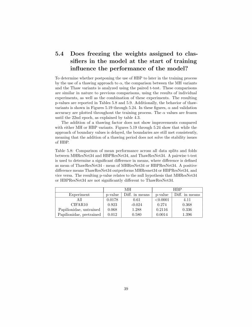
5.4 Does freezing the weights assigned to clas-sifiers in the model at the start of traininginfluence the performance of the model?

To determine whether postponing the use of HBP to later in the training processby the use of a thawing approach to α, the comparison between the MH variantsand the Thaw variants is analyzed using the paired t-test. These comparisonsare similar in nature to previous comparisons, using the results of individualexperiments, as well as the combination of these experiments. The resultingp-values are reported in Tables 5.8 and 5.9. Additionally, the behavior of thaw-variants is shown in Figures 5.19 through 5.24. In these figures, α and validationaccuracy are plotted throughout the training process. The α values are frozenuntil the 22nd epoch, as explained by table 4.3.

The addition of a thawing factor does not show improvements comparedwith either MH or HBP variants. Figures 5.19 through 5.24 show that while theapproach of boundary values is delayed, the boundaries are still met consistently,meaning that the addition of a thawing period does not solve the stability issuesof HBP.

Table 5.8: Comparison of mean performance across all data splits and foldsbetween MHResNet34 and HBPResNet34, and ThawResNet34. A pairwise t-testis used to determine a significant difference in means, where difference is definedas mean of ThawResNet34 - mean of MHResNet34 or HBPResNet34. A positivedifference means ThawResNet34 outperforms MHResnet34 or HBPResNet34, andvice versa. The resulting p-value relates to the null hypothesis that MHResNet34or HBPResNet34 are not significantly different to ThawResNet34.

MH HBPExperiment p-value Diff. in means p-value Diff. in means

All 0.0178 0.61 <0.0001 4.11CIFAR10 0.923 -0.024 0.274 0.368

Papilionidae, untrained 0.068 1.288 0.2116 0.336Papilionidae, pretrained 0.012 0.580 0.0014 1.396

39

Figure 5.19: Results for ThawResNet34 for individual classifiers on 20% oftraining data for CIFAR10. Shown is the validation accuracy over all trainingepochs for each individual classifier and the combined weighted output.

Figure 5.20: Results for ThawDenseNet121 for individual classifiers on 20% oftraining data for CIFAR10. Shown is the validation accuracy over all trainingepochs for each individual classifier and the combined weighted output.

40

Figure 5.21: Results for ThawResNet34 for individual classifiers on 20% oftraining data for Papilionidae, untrained. Shown is the validation accuracyover all training epochs for each individual classifier and the combined weightedoutput.

Figure 5.22: Results for ThawDenseNet121 for individual classifiers on 20%of training data for Papilionidae, untrained. Shown is the validation accuracyover all training epochs for each individual classifier and the combined weightedoutput.

41

Figure 5.23: Results for ThawResNet34 for individual classifiers on 20% oftraining data for Papilionidae, pretrained. Shown is the validation accuracyover all training epochs for each individual classifier and the combined weightedoutput.

Figure 5.24: Results for ThawDenseNet121 for individual classifiers on 20% oftraining data for Papilionidae, pretrained. Shown is the validation accuracyover all training epochs for each individual classifier and the combined weightedoutput.

42

Table 5.9: Comparison of mean performance across all data splits and foldsbetween MHDenseNet121 and HBPDenseNet121, and ThawDenseNet121. Apairwise t-test is used to determine a significant difference in means, wheredifference is defined as mean of ThawDenseNet121 - mean of MHDenseNet121 orHBPDenseNet121. A positive difference means ThawDenseNet121 outperformsMHDenseNet121 or HBPDenseNet121, and vice versa. The resulting p-valuerelates to the null hypothesis that MHDenseNet121 or HBPDenseNet121 are notsignificantly different to ThawDenseNet121.

MH ThawExperiment p-value Diff. in means p-value Diff. in means

All 0.515 -0.104 0.877 -0.023CIFAR10 0.282 -0.384 0.756 0.104

Papilionidae, untrained 0.763 0.092 0.0617 0.468Papilionidae, pretrained 0.874 -0.020 0.0392 0.296

5.5 Do the behaviours of these models changewhen using differing amounts of data?

Figures 5.25 through 5.27 show the performance of each model with increasingdata for each of the experimental settings. From these figures, it is clear that therelative performance of each model does not change significantly when increasingthe amount of training data.

Figure 5.25: Mean results for all models on all folds for CIFAR10, plotted overthe amount of data used.

43

Figure 5.26: Mean results for all models on all folds for Papilionidae, untrained,plotted over the amount of data used.

Figure 5.27: Mean results for all models on all folds for Papilionidae, pretrained,plotted over the amount of data used.

44

Chapter 6

Discussion

The results, as shown in Chapter 5, show several patterns. However, thesepatterns seem to be experiment specific, with the analysis on CIFAR10 differingsignificantly from experiments on Papilionidae, both with and without transferlearning. Therefore, when applicable, the research questions will be answeredwith emphasis on individual experiments, rather than with more generalizablestatements. The results from Chapter 5 are summarized below, before beingfurther discussed.

6.1 Research Questions

Does a model with multiple heads perform better than the basemodel?

From Tables 5.4 and 5.5, it shows that MH variants outperform base variantsonly on CIFAR10. The follow-up question of why this difference between ex-periments occurs leads to Figures 5.1 to 5.6, which shows the effects of the MHvariant on regularizing the training process, providing a more generalizable model.The MH variants are able to optimize better due to a more gradual decreasein the loss and validation accuracy, preventing the early stopping mechanismfrom intervening too aggresively. These effects of more gradual learning andsubsequent performance increase for MH variants do not occur in experimentson the Papilionidae data, both with and without transfer learning. In conclu-sion, the use of MH variants may increase performance on classification tasksusing CNNs compared to a base version. However, this gain varies between tasks.

Do the additional heads increase performance when active during in-ference, in contrast to only using additional heads during training?

From Figures 5.7 and 5.8, it shows that the combined weighted output of theMH model variants slightly outperforms the third, final classifier. In established

45

deep supervision techniques, the early classifiers are removed at inference time,which is similar to looking at the performance of classifier 3 in the MH variant.Because the combined output outperforms the third classifier in the CIFAR10experimental setting, it shows that leaving the additional classifiers active duringinference provides a benefit. This effect was not observed for other experimentalsettings, as for these the MH variant did not outperform the base variant. Therewas no difference in performance between the third classifier and the combinedoutput in the experiments with the Papilionidae dataset, both with and withouttransfer learning.

Does the hedge backpropagation (HBP) algorithm successfully opti-mize weights between output layers of a model with multiple heads?

Tables 5.6 and 5.7 show the difference in performance between MH andHBP variants. From these tables it is clear that the addition of HBP does notimprove the training of the architecture. The differences in performance areeither statistically insignificant, negligibly small, or in favor of the MH variant.Additionally, Figures 5.13 through 5.18 show the development of α in each ofthe experiments. While the development of α throughout training is differentbased on the model and the data used, the end result is that the final classifierreaches the upper bound for α, while all other classifiers reach the lower bound.This indicates that α is unstable and the HBP algorithm is sub-optimal.

Does freezing the weights assigned to classifiers in the model at thestart of training influence the performance of the model? Does thissignificantly differ from the MH or HBP models?

In Tables 5.8 and 5.9, the performance of the Thaw variants is compared toboth MH and HBP variants. Similar to the comparison between MH and HBPvariants, these tables show that any discernible difference in the performance ofthese variants is either statistically insignificant or negligibly small. Figures 5.19through 5.24 show the development of α in Thaw variants for all settings. Fromthese results it shows that the final performance of the model does not increasecompared to either MH or HBP variants for any of the experimental settings.The effect of freezing alpha development for 22 epochs seems to have mainly adelaying effect. The α values for the classifiers do not reach their maximum andminimum value as quickly and in some scenarios the upper and lower bounds arenot reached at all. However, the curve does not seem to flatten yet, indicatingthat the only reason for the bounds not being reached is early stopping, ratherthan a stable distribution for α being reached.

Do the behaviours of these models change when using differing amountsof data?

Shown in Figures 5.25 through 5.27 are the increases in performance permodel when training data is increased. From these figures it shows that the

46

relative performance of different model variants does not change considerablywith different amounts of data. In other words, when looking at Figure 5.25,the base variant consistently performs worse than variants with multiple heads,regardless of amount of training data used. Similarly, there is no difference inrelative performance between variants in Figures 5.26 and 5.27. This shows noindication that using additional classifiers in shallow parts of the model allowsthe model to adapt to the unavailability of data by focusing on the optimizationof a shallower model.

6.2 Conclusions

This work shows the benefits of the Multiple Heads architecture in some, butnot all, scenarios. The established technique of deep supervision has alreadybeen shown to improve training of certain models, and that is verified in thiswork. However, an additional hypothesis arose that in some of the circumstanceswhere deep supervision is beneficial, keeping the additional classifiers intactat inference time may increase model performance to some extent. With thedata provided by experiments in this work, no conclusive statements can bemade about general applicability, but specifically for the CIFAR10 setting asignificant benefit has been observed. The fact that this observation is seen inboth ResNet34 and DenseNet121 puts more weight behind it.

Unfortunately, this is where the benefits of this work stagnate. The explo-ration of a new algorithm to determine weights between heads in the MH modelvariant has been unsuccessful. Both HBP and Thaw variants show no benefits ontop off the benefits from the MH variant. Interesting to note is that the variantsusing an adaptable α also do not appear to hinder the performance. This is likelydue to setting rigorous upper and lower bounds for α, as all figures show thatthe bounds are consistently reached, albeit with a delay in the case of the Thawvariants. This indicates a highly unstable system. Initially the HBP algorithmwas developed not for convolutional neural networks (CNNs), but for Multi-LayerPerceptrons (MLPs) of significant depth [Sahoo et al., 2018]. Additionally, thiswas done in the interest of online deep learning, assuming each sample wouldonly be viewed once. While it is unclear whether these circumstances prevent αfrom reaching its upper and lower bounds, it is intuitive to see that continuousiteration over the same data will push α to extremes as soon as a clear bestclassifier establishes itself. The adaptation to CNNs was based on the idea thatearlier classifiers would be more dominant early on in training, and only diminishin value after a period of time when the final classifier learns all the details ofthe data. However, the empirical results have shown that the final classifier isable to outperform other classifiers from the start, resulting in the α for thisclassifier increasing, its training picking up more speed, which further feeds intoits superiority over the other classifiers. This becomes a feedback loop wherethe final classifier will be dominant throughout all stages of the training process.

If the final classifier outperforms earlier classifiers, why is the MH variant thenable to outperform a base variant? What do the earlier classifiers add to improve

47

the architecture? The additional classifiers appear to help in regularizing thenetwork. This is seen in the convergence behaviour for experiments on CIFAR10,where the more gradual loss curve for MH variants allows the model to surpassthe base variant without interference from the early stopping mechanism. Inother words, the behaviour indicates that the MH adaptation allows the modelto avoid a local minimum that the base variant is more prone to get stuck in.

Addtionally, while both ResNets and DenseNets have their own structures toreduce the effects of the vanishing gradient problem, the fact remains that detailsfrom earlier layers will get lost in the final classification. The addition of earlierclassifiers, as in deep supervision, helps by giving the earlier convolutional blocksmore direct feedback on the features being extracted. As the experimental datashows, for the models tested in this work, and with specific datasets, this helpsto keep the model more generalized at inference time.

Finally, the original work, being developed for online learning, assumed thata system would gradually see more data and adapt to that by using the deeperclassifiers. As such, this work posited the question of whether the behaviouralcomparison between different model variants would change given the amount ofdata used. While this is not the same as online learning, the question is relevantin modern deep learning research due to improvements often being contingenton very large datasets. Having an architecture that would also function withlower amounts of data, or outperform the base net by a larger margin comparedto using a bigger dataset, can be very beneficial. However, the empirical resultsshow that the relative performance of the models does not differ very much evenwith an increase in data by a factor of 20 (5% data compared to 100% data).The performance gap closes somewhat, but that is also attributable to bothbase and MH variants achieving accuracies closer to 100. The reduction in errorremains similar for increasing amounts of data.

6.3 Recommendations for Future Research

The steps towards future research encompass two directions. The first is todetermine the validity of the statements in this work by expanding the field ofview. This means the models developed herein would be applied to numerousdatasets in an attempt to detect a pattern in the type of data these models canhelp with or not. To broaden the field of view, a direct comparison can also bemade between the models developed in this work and other works using auxiliaryheads for deep supervision. These comparisons can focus on the added value ofthe auxiliary heads both at training and inference time. Examples of this includeGoogLeNet [Szegedy et al., 2015] and Inception v3 [Szegedy et al., 2016].

Future work may also focus on expanding the techniques developed in thiswork in order to address the issues inherent to HBP. This can be done by, forexample, developing a model that fully trains the weights until convergencebefore adapting α. This allows each classifier to find its individual optimalcontribution before determining the amount each classifier contributes to theweighted output. One step further would be to take this two-step training

48

process and develop en n-step training process where weight adaptation andalpha adaptation are alternated until some convergence criteria is met.

Alternatively, an architecture can be developed that functions as the reverseof the Thaw variant. In this architecture, the alpha would be adaptable until acertain epoch, basically prohibiting the alpha from always reaching its boundaryvalue by bounding it in the time domain. And a combination of thawing andfreezing α could result in a model that has a static α at the start of training,adapts it after a preset n number of epochs before freezing α again at epoch m,where m > n. These adaptations, however, attempt to shape α in a certain way,and the choices and additional hyper parameters that this entails would veryclosely start to resemble a MH variant with predetermined, possibly non-equal,weights. These variants do not solve the inherent issues with HBP in that itdoes not converge any other way than by reaching the preset upper and lowerbounds.

Theoretically, the HBP variants should outperform MH variants on the simplebasis that if the optimal weighted combination of classifiers is found, these shouldeither be better than a statically weighted ensemble or converge on the sameweights as the statically weighted ensemble. This leads to the idea that this canbe achieved if a stable method of updating α can be found. A start may be touse the log loss instead of the real loss, such that the discrepancy between largelosses at the start and small losses at the end of training are smoothed. Thisdifference in size of the loss directly affects α calculation and smoothing it maybalance impact of α updates from early and late in the training process. Ofcourse, further algorithms can be developed which adapt α in an online fashion,and these heavily influence the comparison between HBP and MH variants ifapplied, but developing these is beyond the scope of this work.

Finally, an interesting point for future research is to revisit two of the decisionsmade early in development. The first of these is the choice to use small versionsof both ResNet and DenseNet. It is argued that this would limit the spacebetween classifiers, i.e. by limiting the convolutional layers per block. However,during development and testing it became clear that the opposite could beequally interesting. By using a network with large blocks, in a similar blockstructure to the architectures in this work, the classifiers are each responsiblefor updating a larger portion of the network. This would increase the severityof the vanishing gradient problem and the disconnect between early layers andthe final classification. As such, in these deeper, harder to train networks, theimpact of additional classifiers might be more noticeable than in the relativelyshallow networks used in this work.

Second, there is the decision to limit the architecture to 3 classifiers. Thisdecision was partly based on computational limitations and partly on early ob-servations during development. These early observations pointed in the directionthat classifiers attached to convolutional layers before the point where the firstclassifier is currently attached would only hinder performance by confusing thepurpose of these early layers. However, in combination with the previous point,when using larger convolutional blocks, resulting in larger amounts of encoderlayers, classifiers placed between the currently used classifiers may add additional

49

value without confusing early layers. To do this, the block structure as describedin Section 3.2 has to let go to some extent, but it could be interesting to explorethis nonetheless.

In closing: The pessimist might say that the architectures developed hereare of little value, adding minor performance in a limited set of circumstances.The optimist might say that gain has been found and the search for a new andbetter architecture was a success. The realist, however, will say that neither thegood nor the bad is conclusive and there is much room for further work.

50

Bibliography

[Dietterich, 2000] Dietterich, T. G. (2000). Ensemble methods in machine learn-ing. In Multiple Classifier Systems, pages 1–15, Berlin, Heidelberg. SpringerBerlin Heidelberg.

[Freund and Schapire, 1997] Freund, Y. and Schapire, R. E. (1997). A decision-theoretic generalization of on-line learning and an application to boosting.Journal of Computer and System Sciences, 55(1):119 – 139.

[Gertych et al., 2019] Gertych, A., Swiderska-Chadaj, Z., Ma, Z., Ing, N.,Markiewicz, T., Cierniak, S., Salemi, H., Guzman, S., Walts, A., and Knudsen,B. (2019). Convolutional neural networks can accurately distinguish fourhistologic growth patterns of lung adenocarcinoma in digital slides. ScientificReports, 9.

[He et al., 2016] He, K., Zhang, X., Ren, S., and Sun, J. (2016). Deep residuallearning for image recognition. 2016 IEEE Conference on Computer Visionand Pattern Recognition (CVPR), pages 770–778.

[Hochreiter, 1991] Hochreiter, S. (1991). Untersuchungen zu dynamischen neu-ronalen netzen.

[Huang et al., 2017a] Huang, G., Li, Y., Pleiss, G., Liu, Z., Hopcroft, J. E., andWeinberger, K. Q. (2017a). Snapshot ensembles: Train 1, get m for free.ArXiv, abs/1704.00109.

[Huang et al., 2017b] Huang, G., Liu, Z., and Weinberger, K. Q. (2017b).Densely connected convolutional networks. 2017 IEEE Conference on Com-puter Vision and Pattern Recognition (CVPR), pages 2261–2269.

[Kolen and Kremer, 2001] Kolen, J. F. and Kremer, S. C. (2001). Gradient flowin recurrent nets: The difficulty of learning longterm dependencies. In A FieldGuide to Dynamical Recurrent Networks, pages 237–243.

[Krizhevsky, 2009] Krizhevsky, A. (2009). Learning multiple layers of featuresfrom tiny images. University of Toronto, pages 32–33.

[Krizhevsky et al., 2012] Krizhevsky, A., Sutskever, I., and Hinton, G. E. (2012).Imagenet classification with deep convolutional neural networks. In Pereira,

51

F., Burges, C. J. C., Bottou, L., and Weinberger, K. Q., editors, Advances inNeural Information Processing Systems, volume 25. Curran Associates, Inc.

[Lecun et al., 1998] Lecun, Y., Bottou, L., Bengio, Y., and Haffner, P. (1998).Gradient-based learning applied to document recognition. Proceedings of theIEEE, 86(11):2278–2324.

[Lee et al., 2015] Lee, C.-Y., Xie, S., Gallagher, P., Zhang, Z., and Tu, Z. (2015).Deeply-Supervised Nets. In Proceedings of the Eighteenth International Con-ference on Artificial Intelligence and Statistics, volume 38 of Proceedings ofMachine Learning Research, pages 562–570.

[Li et al., 2019] Li, C., Zia, M. Z., Tran, Q.-H., Yu, X., Hager, G., and Chan-draker, M. (2019). Deep supervision with intermediate concepts. IEEETransactions on Pattern Analysis and Machine Intelligence, 41:1828–1843.

[Marre et al., 2020] Marre, G., De Almeida Braga, C., Ienco, D., Luque, S.,Holon, F., and Deter, J. (2020). Deep convolutional neural networks to monitorcoralligenous reefs: Operationalizing biodiversity and ecological assessment.Ecological Informatics, 59:101110.

[Minetto et al., 2019] Minetto, R., Segundo, M. P., and Sarkar, S. (2019). Hydra:An ensemble of convolutional neural networks for geospatial land classification.IEEE Transactions on Geoscience and Remote Sensing, 57:6530–6541.

[Naturalis Biodiversity Center, 2021] Naturalis Biodiversity Center (2021). Pa-pilionidae specimens.

[Paszke et al., 2019] Paszke, A., Gross, S., Massa, F., Lerer, A., Bradbury, J.,Chanan, G., Killeen, T., Lin, Z., Gimelshein, N., Antiga, L., Desmaison,A., Kopf, A., Yang, E., DeVito, Z., Raison, M., Tejani, A., Chilamkurthy,S., Steiner, B., Fang, L., Bai, J., and Chintala, S. (2019). Pytorch: Animperative style, high-performance deep learning library. In Advances in NeuralInformation Processing Systems 32, pages 8024–8035. Curran Associates, Inc.

[Rosenblatt, 1958] Rosenblatt, F. (1958). The perceptron: a probabilistic modelfor information storage and organization in the brain. Psychological review,65 6:386–408.

[Rumelhart et al., 1986] Rumelhart, D. E., Hinton, G. E., and Williams, R. J.(1986). Learning Representations by Back-propagating Errors. Nature,323(6088):533–536.

[Sahoo et al., 2018] Sahoo, D., Pham, Q., Lu, J., and Hoi, S. C. H. (2018). Onlinedeep learning: Learning deep neural networks on the fly. In Proceedings ofthe Twenty-Seventh International Joint Conference on Artificial Intelligence,IJCAI-18, pages 2660–2666. International Joint Conferences on ArtificialIntelligence Organization.

52

[Shen et al., 2020] Shen, Z., Liu, Z., Li, J., Jiang, Y. G., Chen, Y., and Xue,X. (2020). Object detection from scratch with deep supervision. IEEETransactions on Pattern Analysis and Machine Intelligence, 42(2):398–412.

[Sigcha et al., 2021] Sigcha, L. F., Pavon, I., Costa, N., Costa, S., Gago, M.,Arezes, P., Lopez Navarro, J. M., and Arcas, G. (2021). Automatic restingtremor assessment in parkinson’s disease using smartwatches and multitaskconvolutional neural networks. Sensors, 21:291.

[Simonyan and Zisserman, 2015] Simonyan, K. and Zisserman, A. (2015). Verydeep convolutional networks for large-scale image recognition. In Bengio, Y.and LeCun, Y., editors, 3rd International Conference on Learning Represen-tations, ICLR 2015, San Diego, CA, USA, May 7-9, 2015, Conference TrackProceedings.

[Sun et al., 2019] Sun, D., Yao, A., Zhou, A., and Zhao, H. (2019). Deeply-supervised knowledge synergy. In 2019 IEEE/CVF Conference on ComputerVision and Pattern Recognition (CVPR), pages 6990–6999.

[Szegedy et al., 2015] Szegedy, C., Liu, W., Jia, Y., Sermanet, P., Reed, S.,Anguelov, D., Erhan, D., Vanhoucke, V., and Rabinovich, A. (2015). Goingdeeper with convolutions. In The IEEE Conference on Computer Vision andPattern Recognition (CVPR), pages 1–9.

[Szegedy et al., 2016] Szegedy, C., Vanhoucke, V., Ioffe, S., Shlens, J., andWojna, Z. (2016). Rethinking the inception architecture for computer vision.In 2016 IEEE Conference on Computer Vision and Pattern Recognition,CVPR 2016, Las Vegas, NV, USA, June 27-30, 2016, pages 2818–2826. IEEEComputer Society.

[Wang et al., 2015] Wang, L., Lee, C.-Y., Tu, Z., and Lazebnik, S. (2015).Training deeper convolutional networks with deep supervision. ArXiv,abs/1505.02496.

[Xu et al., 2015] Xu, B., Wang, N., Chen, T., and Li, M. (2015). Empirical evalu-ation of rectified activations in convolutional network. CoRR, abs/1505.00853.

[Ye et al., 2017] Ye, C., Yang, Y., Mao, R., Fermuller, C., and Aloimonos, Y.(2017). What can i do around here? deep functional scene understanding forcognitive robots. In 2017 IEEE International Conference on Robotics andAutomation (ICRA), pages 4604–4611.

[Yutong and Zhao, 2015] Yutong, S. and Zhao, H. (2015). Stock selection modelbased on advanced adaboost algorithm. In 2015 7th International Conferenceon Modelling, Identification and Control (ICMIC), pages 1–7.

[Zhou et al., 2002] Zhou, Z.-H., Wu, J., and Tang, W. (2002). Ensembling neuralnetworks: Many could be better than all. Artificial Intelligence, 137(1):239–263.

53

Chapter 7

Appendix A - Full Results

Table 7.1: CIFAR10: Validation accuracy for all models on the CIFAR10 datasetusing 5% of training data. Best performing variant per base model is shown inbold.

Model Fold 1 Fold 2 Fold 3 Fold 4 Fold 5 MeanResNet34 61.3 60.6 62.5 62.9 63.3 62.1

MHResNet34 68.4 64.6 67.3 65.6 66.8 66.5HBPResNet34 64.4 61.8 66.8 66.6 64.3 64.8ThawResNet34 67.7 63.8 65.9 64.0 69.9 66.3

Densenet121 63.0 62.9 63.4 63.1 65.9 63.7MHDenseNet121 66.7 67.0 67.6 63.8 65.6 66.1HBPDenseNet121 67.2 65.4 63.5 64.5 62.6 64.6ThawDenseNet121 62.4 64.2 62.8 66.9 64.3 64.1

54













55

Table 7.5: CIFAR10: Validation accuracy for all models on the CIFAR10 datasetusing 100% of training data. Best performing variant per base model is shownin bold.




Table 7.6: Validation accuracy for all models on the Papilionidae dataset using5% of training data. Best performing variant per base model is shown in bold.








56













57

Table 7.11: Validation accuracy for all models, pretrained on ImageNet, on thePapilionidae dataset using 5% of training data. Best performing variant per basemodel is shown in bold.




Table 7.12: Validation accuracy for all models, pretrained on ImageNet, on thePapilionidae dataset using 10% of training data. Best performing variant perbase model is shown in bold.








58









59

hedge backpropagation in convolutional neural networks

Documents