Tackling Class Imbalance with Deep Convolutional Neural Networks— Final —

Alexandre Dalyac, Prof Murray Shanahan, Jack Kelly; Imperial College London

September 24, 2014

Abstract

Automatic image classification experienced a breakthrough in 2012 with the advent of GPU im-plementations of deep convolutional neural networks (CNNs). These models distinguish themselvesby learning features, convolving them to achieve feature equivariance, making use of max poolingoperations to achieve robustness to cluttered backgrounds, and a hierarchical structure to enablethe learning of complex features with high generalisation performance.

This report provides an overview of supervised deep learning, followed by an in-depth explana-tion of the workings of a deep convolutional neural network, which despite its performance, gatherscriticism for its tendency to be used as a black box. The rest of the report goes over the researchthat was carried out. The first is a simple mathematical analysis which proposes an explanation forthe recent success of the Rectified Linear Unit as the chief activation function of CNNs. The nextsections are applied: understanding why learning fails with class imbalance and noisy labels, andexploring ways of tackling it – including a novel cost function with a probabilistic interpretationwhich delivered up to 25 additional percentage points in classification performance.

2nd September 2014

Contents

1 Acknowledgements 4

2 Introduction 52.0.1 Data Overview . . . . . . . . . . . . . . . . . . . . . . . . . . . . . . . . . . . . 52.0.2 Semantic Complexity . . . . . . . . . . . . . . . . . . . . . . . . . . . . . . . . 52.0.3 Domain Change . . . . . . . . . . . . . . . . . . . . . . . . . . . . . . . . . . . 62.0.4 Small Dataset Size . . . . . . . . . . . . . . . . . . . . . . . . . . . . . . . . . . 62.0.5 Class Imbalance . . . . . . . . . . . . . . . . . . . . . . . . . . . . . . . . . . . 7

3 Literature Review 83.1 Supervised Learning . . . . . . . . . . . . . . . . . . . . . . . . . . . . . . . . . . . . . 83.2 Approximation vs Generalisation . . . . . . . . . . . . . . . . . . . . . . . . . . . . . . 83.3 Models of Neurons . . . . . . . . . . . . . . . . . . . . . . . . . . . . . . . . . . . . . . 83.4 Feed-forward Architecture . . . . . . . . . . . . . . . . . . . . . . . . . . . . . . . . . . 113.5 Justifying Depth . . . . . . . . . . . . . . . . . . . . . . . . . . . . . . . . . . . . . . . 123.6 Backpropagation . . . . . . . . . . . . . . . . . . . . . . . . . . . . . . . . . . . . . . . 14

3.6.1 Compute Error-Weight Partial Derivatives . . . . . . . . . . . . . . . . . . . . . 143.6.2 Update Weight Values with Gradient Descent . . . . . . . . . . . . . . . . . . . 143.6.3 Stochastic Gradient Descent . . . . . . . . . . . . . . . . . . . . . . . . . . . . . 14

3.7 Overfit . . . . . . . . . . . . . . . . . . . . . . . . . . . . . . . . . . . . . . . . . . . . . 143.7.1 Cross Validation . . . . . . . . . . . . . . . . . . . . . . . . . . . . . . . . . . . 153.7.2 Data Augmentation . . . . . . . . . . . . . . . . . . . . . . . . . . . . . . . . . 163.7.3 Dropout . . . . . . . . . . . . . . . . . . . . . . . . . . . . . . . . . . . . . . . . 16

3.8 Deep Convolutional Neural Networks . . . . . . . . . . . . . . . . . . . . . . . . . . . . 183.8.1 Pixel Feature . . . . . . . . . . . . . . . . . . . . . . . . . . . . . . . . . . . . . 193.8.2 Non-linear Activation . . . . . . . . . . . . . . . . . . . . . . . . . . . . . . . . 213.8.3 Pooling aka Spatial Feature . . . . . . . . . . . . . . . . . . . . . . . . . . . . . 213.8.4 Contrast Normalisation . . . . . . . . . . . . . . . . . . . . . . . . . . . . . . . 21

3.9 Local vs Global Optimisation . . . . . . . . . . . . . . . . . . . . . . . . . . . . . . . . 223.10 Transfer Learning . . . . . . . . . . . . . . . . . . . . . . . . . . . . . . . . . . . . . . . 23

3.10.1 Linear Support Vector Machines . . . . . . . . . . . . . . . . . . . . . . . . . . 233.11 Class Imbalance . . . . . . . . . . . . . . . . . . . . . . . . . . . . . . . . . . . . . . . . 23

4 Analysis 1: ReLU Activation 254.1 Motivations . . . . . . . . . . . . . . . . . . . . . . . . . . . . . . . . . . . . . . . . . . 254.2 Mathematical Analysis . . . . . . . . . . . . . . . . . . . . . . . . . . . . . . . . . . . . 26

4.2.1 How the Gradient Propagates . . . . . . . . . . . . . . . . . . . . . . . . . . . . 264.2.2 An Example . . . . . . . . . . . . . . . . . . . . . . . . . . . . . . . . . . . . . 264.2.3 Vanishing Gradient . . . . . . . . . . . . . . . . . . . . . . . . . . . . . . . . . . 274.2.4 Impact of the ReLU . . . . . . . . . . . . . . . . . . . . . . . . . . . . . . . . . 28

5 Experiments 1: Identifying Class Imbalance 305.1 Implementation: Cuda-Convnet . . . . . . . . . . . . . . . . . . . . . . . . . . . . . . . 305.2 Experimentation . . . . . . . . . . . . . . . . . . . . . . . . . . . . . . . . . . . . . . . 30

5.2.1 Non-Converging Error Rates . . . . . . . . . . . . . . . . . . . . . . . . . . . . 305.2.2 Increase Validation Error Precision . . . . . . . . . . . . . . . . . . . . . . . . . 315.2.3 Periodicity of the training error . . . . . . . . . . . . . . . . . . . . . . . . . . . 325.2.4 Poor, Sampling-Induced Corner Minima . . . . . . . . . . . . . . . . . . . . . . 325.2.5 Mislabelling . . . . . . . . . . . . . . . . . . . . . . . . . . . . . . . . . . . . . . 34

2

2nd September 2014

6 Experiments 2: Tackling Class Imbalance 366.1 Definition . . . . . . . . . . . . . . . . . . . . . . . . . . . . . . . . . . . . . . . . . . . 366.2 Motivations . . . . . . . . . . . . . . . . . . . . . . . . . . . . . . . . . . . . . . . . . . 366.3 Implementation . . . . . . . . . . . . . . . . . . . . . . . . . . . . . . . . . . . . . . . . 376.4 Experimentation . . . . . . . . . . . . . . . . . . . . . . . . . . . . . . . . . . . . . . . 37

6.4.1 Test Run . . . . . . . . . . . . . . . . . . . . . . . . . . . . . . . . . . . . . . . 376.4.2 Transfer Learning . . . . . . . . . . . . . . . . . . . . . . . . . . . . . . . . . . 396.4.3 Hyperparameter Optimisation . . . . . . . . . . . . . . . . . . . . . . . . . . . . 396.4.4 Over-Sampling . . . . . . . . . . . . . . . . . . . . . . . . . . . . . . . . . . . . 416.4.5 Under-Sampling . . . . . . . . . . . . . . . . . . . . . . . . . . . . . . . . . . . 416.4.6 Threshold-Moving . . . . . . . . . . . . . . . . . . . . . . . . . . . . . . . . . . 446.4.7 Bayesian Cross Entropy Cost Function . . . . . . . . . . . . . . . . . . . . . . . 456.4.8 Error-accuracy mismatch revisited . . . . . . . . . . . . . . . . . . . . . . . . . 49

7 Conclusions and Future Work 50

3

2nd September 2014

1 Acknowledgements

Many thanks to Prof Murray Shanahan for having been the chief supervisor of this researchproject; it would not have been possible to pursue it otherwise.

Thanks to Jack Kelly, the second supervisor of this project, for having created it. Were it not forhim I would not have been able to carry out exciting, meaningful research for a real world problem.

Thanks to Razvan Ranca for precious strategic advice on which experiments to choose for theexploration of hypotheses, help with C++, feedback on the report, as well as musical and caffeinetricks for staying up all night. I look excitingly forward to the times ahead cofounding a machinelearning startup together.

Thanks to Alexandre de Brebisson for his great insights into convnet architecture that helped memake sense of experimental results, and the great conversations we had sharing our passion for deeplearning.

The Google+ Deep Learning community was perhaps the 2nd most precious resource for thisproject, after arXiv and before stackoverflow. It provided a large and steady stream of useful resources,comments and guidance. It also seemed like a revolutionary way to be in touch with the world’s leadingresearchers such as Prof Yann LeCun and Prof Yoshua Bengio. I owe particular thanks to Dr SoumithChintala for his comments on transfer learning and Prof Francisco Zamora-Martinez for his on classimbalance.

4

2nd September 2014

2 Introduction

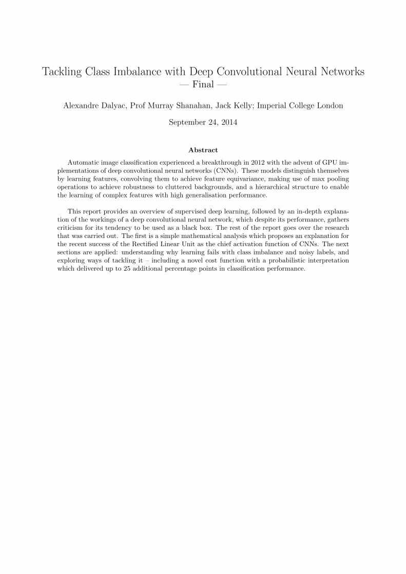
A number of significant challenges arise from this task: multi-tagging, semantic complexity, do-main change, small dataset size and class imbalance. Before going into them, an overview of the datais given on figure 1.

2.0.1 Data Overview

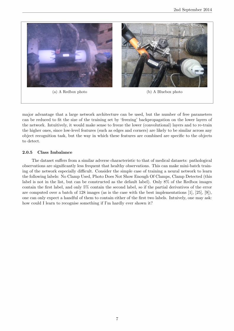
ControlPoint recently upgraded the photographical equipment with which photos are taken (from’Redbox’ equipment to ’Bluebox’ equipment), which means that the resolution and finishing of thephotos has been altered. There are 113,865 640x480 ’RedBox’ images. There are 13,790 1280x960’BlueBox’ images. Label frequencies for the Redbox images are shown on figure 1.

Characteristic Redbox Count Bluebox Count

Fitting Proximity 1,233 32Inadequate Or Incorrect Clamping 1,401 83Joint Misaligned 391 35No Clamp Used 8,041 1,571No Ground Sheet 30,015 5,541No Insertion Depth Markings 17,667 897No Visible Evidence Of Scraping Or Peeling 25,499 1,410No Visible Hatch Markings 28,155 3,793Other 251 103Photo Does Not Show Enough Of Clamps 5,059 363Photo Does Not Show Enough Of Scrape Zones 21,272 2,545Soil Contamination High Risk 6,541 3Soil Contamination Low Risk 10 N/ASoil Contamination Risk ? 529Unsuitable Photo 2 N/AUnsuitable Scraping Or Peeling 2,125 292Water Contamination High Risk 1,927 9Water Contamination Low Risk 3 7Water Contamination Risk ? 296

Perfect (no labels) 49,039 4,182

Table 1: Count of Redbox images with given label

2.0.2 Semantic Complexity

Certain visual characteristics are semantically more complex than normal object classes, becauseControlPoint has rules for what counts to raise a flag depending on the nature of the joint. For ex-ample, in the case of clamp detection, for tapping-T joints, for the Redbox images, the glint of a slimportion of a clamp is sufficient to judge it present. An example is shown on figure 1.

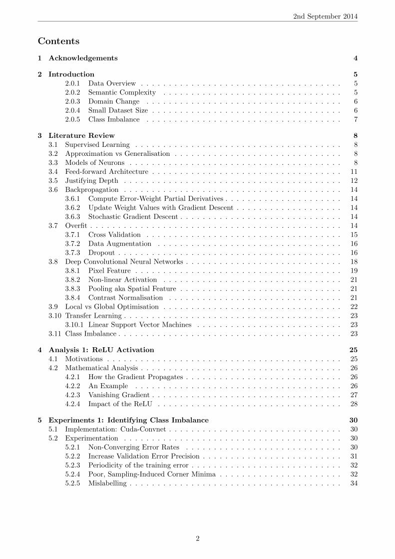
Worse still, sometimes the presence of clamps ‘does not count’: these are cases for which thepurpose of the clamp is other than to secure the welding. Therefore, if such a clamp is present, butthe clamp that serves to secure the weld is absent, then the image is assigned the ‘No Clamps’ label.For example, bottom left, a clamp can clearly be seen, but it’s not a weld clamp. So this imageshould have a ‘No Clamps’ flag raised (sadly, it doesn’t). Bottom right: the thin metallic clamp thatis fastened on the vertical pipe is not the clamp we’re interested in. The glint from the thin metallicrod going along the thick, horizontal pipe tells us that a tapping-T clamp is present, even though thatclamp is hidden underneath the pipe. An example is shown on figure ??.

5

2nd September 2014

Figure 1: The clamp wraps around under the pipe - the glint of a metal rod gives it away

(a) The clamp is not a weld clamp (b) The clamp on the vertical rod is not a weld clamp

2.0.3 Domain Change

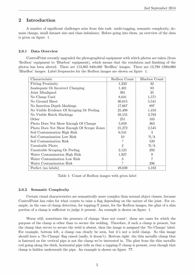
Domain change can be lethal to computer vision algorithms: for example, a feature learned (atthe pixel level) from the 640x480 Redbox images could end up being out of scale for the 1280x960Bluebox images. However, this simple example is not relevant to a CNN implementation, since thelargest networks can only manage 256x256 images, so Bluebox and Redbox images will both bedownsized to identical resolutions. However, of greater concern is the difference in image sharpnessbetween Redbox and Bluebox images, as can be seen on figure ??. It remains to be seen how a CNNcould be made to deal with this type of domain change.

Nevertheless, evidence has been found to suggest that deep neural networks are robust to it: anexperiment run by Donahue et al on the Office dataset [22], consisting of images of the same productstaken with three different types of photographical equipment (professional studio equipment, digitalSLR, webcam) found that their implementation of a deep convolutional neural network produced simi-lar feature representations of two images of the same object even when the two images were taken withdifferent equipment, but that this was not the case when using SURF, the currently best performingset of hand-coded features on the Office dataset [24].

2.0.4 Small Dataset Size

Alex Krizhevsky’s record-breaking CNN was trained on 1 million images [1]. Such a large datasetenabled the training of a 60-million parameter neural network, without leading to overfit. In this case,there are ’only’ 5,000, and 43% of them are images of ‘perfect’ welds, meaning that these are label-less.Training a similarly sized network leads to overfit, but training a smaller network could prevent thenetwork from learning sufficiently abstract and complex features for the task at hand. A solution toconsider is that of transfer learning [25], which consists in importing a net which has been pretrainedin a similar task with vast amounts of data, and to use it as a feature extractor. This would bring the

6

2nd September 2014

(a) A Redbox photo (b) A Bluebox photo

major advantage that a large network architecture can be used, but the number of free parameterscan be reduced to fit the size of the training set by ‘freezing’ backpropagation on the lower layers ofthe network. Intuitively, it would make sense to freeze the lower (convolutional) layers and to re-trainthe higher ones, since low-level features (such as edges and corners) are likely to be similar across anyobject recognition task, but the way in which these features are combined are specific to the objectsto detect.

2.0.5 Class Imbalance

The dataset suffers from a similar adverse characteristic to that of medical datasets: pathologicalobservations are significantly less frequent that healthy observations. This can make mini-batch train-ing of the network especially difficult. Consider the simple case of training a neural network to learnthe following labels: No Clamp Used, Photo Does Not Show Enough Of Clamps, Clamp Detected (thislabel is not in the list, but can be constructed as the default label). Only 8% of the Redbox imagescontain the first label, and only 5% contain the second label, so if the partial derivatives of the errorare computed over a batch of 128 images (as is the case with the best implementations [1], [25], [9]),one can only expect a handful of them to contain either of the first two labels. Intuively, one may ask:how could I learn to recognise something if I’m hardly ever shown it?

7

2nd September 2014

3 Literature Review

3.1 Supervised Learning

Learning in the case of classification consists in using the dataset D to find the hypothesis functionfh that best approximates the unknown function f∗ : 2X → 2Y which would perfectly classify anysubset of the instance space X . Supervised learning arises when f∗(x) is known for every instance in thedataset, i.e. when the dataset is labelled and of the form (x1, f

∗(x1)), (x2, f∗(x2)), ..., (xn, f

∗(xn)).This means that |D| points of f∗ are known, and can be used to fit fh to them, using an appropriatecost function C. D is therefore referred to as the training set.

Formally, supervised learning therefore consists in finding

fh = argminF

C(D) (1)

where F is the chosen target function space in which to search for fh .

3.2 Approximation vs Generalisation

It is important to note that supervised learning does not consist in merely finding the functionwhich best fits the training set - the availability of numerous universal approximating function classes(such as the set of all finite order polynomials) would make this a relatively simple task [16]. Thecrux of supervised learning is to find a hypothesis function which fits the training set well and wouldfit well to any subset of the instance space, including unseen data. Approximation and generalisationtogether make up the two optimisation criteria for supervised learning.

3.3 Models of Neurons

Learning a hypothesis function fh comes down to searching a target function space for thefunction which minimises the cost function. A function space is defined by a parametrised functionequation, and a parameter space. Choosing a deep convolutional neural network with rectified linearneurons sets the parametrised function equation. By explaining the architecture of such a neuralnetwork, this subsection justifies the chosen function equation. As for the parameter space, it is RP

(where P is the number of parameters in the network); its continuity must be noted as this enablesthe use of gradient descent as the optimisation algorithm (as is discussed later).

Before we consider the neural network architecture as a whole, let us start with the building blockof a neural network: the neuron (mathematically referred to as the activation function). Two typesof neuron models are used in current state-of-the-art implementations of deep convolutional neuralnetworks: the rectified linear unit and the softmax unit (note that the terms ‘neuron’ and ‘unit’ areused interchangeably). In order to bring out their specific characteristics, we shall first consider twoother compatible neuron models: the binary threshold neuron, which is the most intuitive, and thehyperbolic tangent neuron, which is the most analytically appealing. It may also help to know whatis being modelled, so a very brief look at a biological neuron shall first be given.

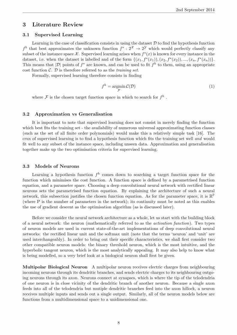
Multipolar Biological Neuron A multipolar neuron receives electric charges from neighbouringincoming neurons through its dendritic branches, and sends electric charges to its neighbouring outgo-ing neurons through its axon. Neurons connect at synapses, which is where the tip of the telodendriaof one neuron is in close vicinity of the dendritic branch of another neuron. Because a single axonfeeds into all of the telodendria but mutiple dendritic branches feed into the axon hillock, a neuronreceives multiple inputs and sends out a single output. Similarly, all of the neuron models below arefunctions from a multidimensional space to a unidimensional one.

8

2nd September 2014

Figure 4: a multipolar biological neuron

Binary Threshold Neuron

y =

1 if M <= b+k∑

i=1xi · wi , where M is a threshold parameter

0 otherwise

(2)

Intuitively, y takes a hard decision, just like biological neurons: either a charge is sent, or it isn’t.y can be seen as producing spikes, xi as the indicator value of some feature, and w[i] as a parameterof the function that indicates how important xi is in determining y. Although this model is closerthan most most to reality, the function is not differentiable, which makes it impossible to use greedylocal optimisation learning algorithms - such as gradient descent - which need to compute derivativesinvolving the activation functions.

Logistic Sigmoid Neuron

y =1

1 + exp(−z), where z =

k∑i=1

xi · wi (3)

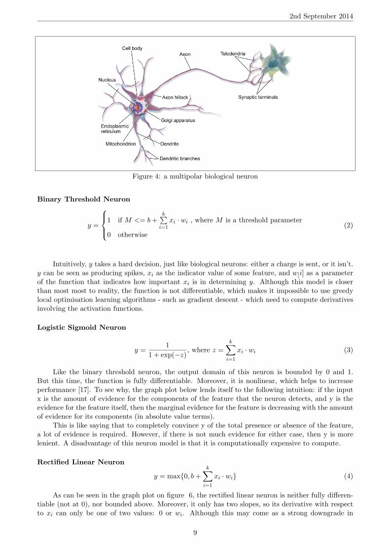
Like the binary threshold neuron, the output domain of this neuron is bounded by 0 and 1.But this time, the function is fully differentiable. Moreover, it is nonlinear, which helps to increaseperformance [17]. To see why, the graph plot below lends itself to the following intuition: if the inputx is the amount of evidence for the components of the feature that the neuron detects, and y is theevidence for the feature itself, then the marginal evidence for the feature is decreasing with the amountof evidence for its components (in absolute value terms).

This is like saying that to completely convince y of the total presence or absence of the feature,a lot of evidence is required. However, if there is not much evidence for either case, then y is morelenient. A disadvantage of this neuron model is that it is computationally expensive to compute.

Rectified Linear Neuron

y = max0, b+k∑

i=1

xi · wi (4)

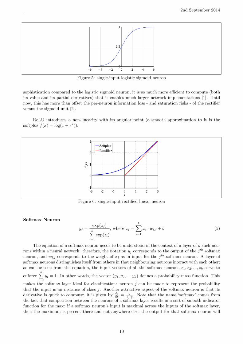
As can be seen in the graph plot on figure 6, the rectified linear neuron is neither fully differen-tiable (not at 0), nor bounded above. Moreover, it only has two slopes, so its derivative with respectto xi can only be one of two values: 0 or wi. Although this may come as a strong downgrade in

9

2nd September 2014

Figure 5: single-input logistic sigmoid neuron

sophistication compared to the logistic sigmoid neuron, it is so much more efficient to compute (bothits value and its partial derivatives) that it enables much larger network implementations [1]. Untilnow, this has more than offset the per-neuron information loss - and saturation risks - of the rectifierversus the sigmoid unit [2].

ReLU introduces a non-linearity with its angular point (a smooth approximation to it is thesoftplus f(x) = log(1 + ex)).

Figure 6: single-input rectified linear neuron

Softmax Neuron

yj =exp(zj)k∑

i=1exp(zi)

, where zj =k∑

i=1

xi · wi,j + b (5)

The equation of a softmax neuron needs to be understood in the context of a layer of k such neu-rons within a neural network: therefore, the notation yj corresponds to the output of the jth softmaxneuron, and wi,j corresponds to the weight of xi as in input for the jth softmax neuron. A layer ofsoftmax neurons distinguishes itself from others in that neighbouring neurons interact with each other:as can be seen from the equation, the input vectors of all the softmax neurons z1, z2, ..., zk serve to

enforcek∑

i=1yi = 1. In other words, the vector (y1, y2, ..., yk) defines a probability mass function. This

makes the softmax layer ideal for classification: neuron j can be made to represent the probabilitythat the input is an instance of class j. Another attractive aspect of the softmax neuron is that itsderivative is quick to compute: it is given by dy

dz = y1−y . Note that the name ‘softmax’ comes from

the fact that competition between the neurons of a softmax layer results in a sort of smooth indicatorfunction for the max: if a softmax neuron’s input is maximal across the inputs of the softmax layer,then the maximum is present there and not anywhere else; the output for that softmax neuron will

10

2nd September 2014

be close to 1 and the output for the other neurons will be close to zero.

3.4 Feed-forward Architecture

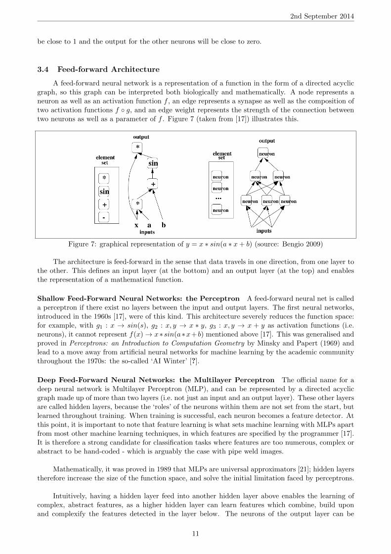
A feed-forward neural network is a representation of a function in the form of a directed acyclicgraph, so this graph can be interpreted both biologically and mathematically. A node represents aneuron as well as an activation function f , an edge represents a synapse as well as the composition oftwo activation functions f g, and an edge weight represents the strength of the connection betweentwo neurons as well as a parameter of f . Figure 7 (taken from [17]) illustrates this.

Figure 7: graphical representation of y = x ∗ sin(a ∗ x+ b) (source: Bengio 2009)

The architecture is feed-forward in the sense that data travels in one direction, from one layer tothe other. This defines an input layer (at the bottom) and an output layer (at the top) and enablesthe representation of a mathematical function.

Shallow Feed-Forward Neural Networks: the Perceptron A feed-forward neural net is calleda perceptron if there exist no layers between the input and output layers. The first neural networks,introduced in the 1960s [17], were of this kind. This architecture severely reduces the function space:for example, with g1 : x → sin(s), g2 : x, y → x ∗ y, g3 : x, y → x + y as activation functions (i.e.neurons), it cannot represent f(x)→ x∗sin(a∗x+ b) mentioned above [17]. This was generalised andproved in Perceptrons: an Introduction to Computation Geometry by Minsky and Papert (1969) andlead to a move away from artificial neural networks for machine learning by the academic communitythroughout the 1970s: the so-called ‘AI Winter’ [?].

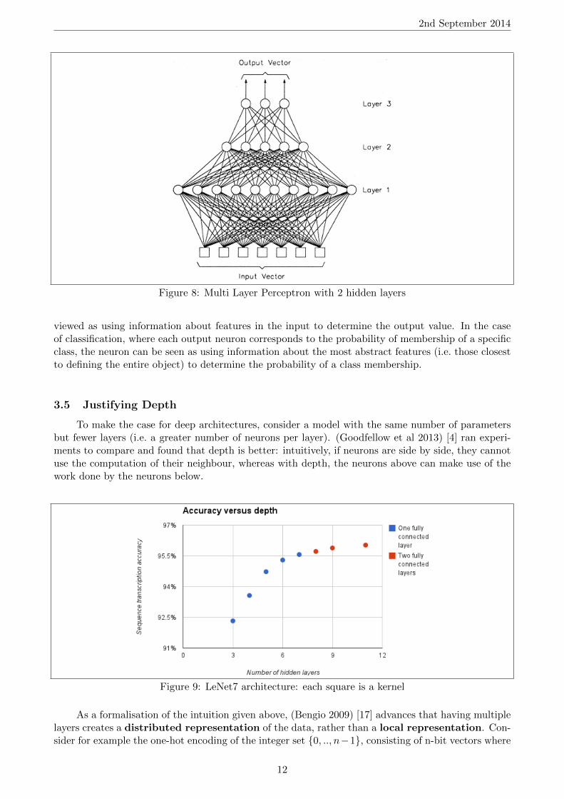
Deep Feed-Forward Neural Networks: the Multilayer Perceptron The official name for adeep neural network is Multilayer Perceptron (MLP), and can be represented by a directed acyclicgraph made up of more than two layers (i.e. not just an input and an output layer). These other layersare called hidden layers, because the ‘roles’ of the neurons within them are not set from the start, butlearned throughout training. When training is successful, each neuron becomes a feature detector. Atthis point, it is important to note that feature learning is what sets machine learning with MLPs apartfrom most other machine learning techniques, in which features are specified by the programmer [17].It is therefore a strong candidate for classification tasks where features are too numerous, complex orabstract to be hand-coded - which is arguably the case with pipe weld images.

Mathematically, it was proved in 1989 that MLPs are universal approximators [21]; hidden layerstherefore increase the size of the function space, and solve the initial limitation faced by perceptrons.

Intuitively, having a hidden layer feed into another hidden layer above enables the learning ofcomplex, abstract features, as a higher hidden layer can learn features which combine, build uponand complexify the features detected in the layer below. The neurons of the output layer can be

11

2nd September 2014

Figure 8: Multi Layer Perceptron with 2 hidden layers

viewed as using information about features in the input to determine the output value. In the caseof classification, where each output neuron corresponds to the probability of membership of a specificclass, the neuron can be seen as using information about the most abstract features (i.e. those closestto defining the entire object) to determine the probability of a class membership.

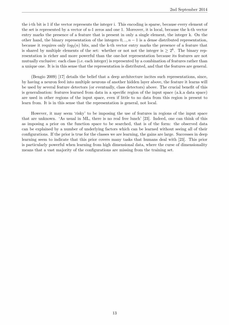
3.5 Justifying Depth

To make the case for deep architectures, consider a model with the same number of parametersbut fewer layers (i.e. a greater number of neurons per layer). (Goodfellow et al 2013) [4] ran experi-ments to compare and found that depth is better: intuitively, if neurons are side by side, they cannotuse the computation of their neighbour, whereas with depth, the neurons above can make use of thework done by the neurons below.

Figure 9: LeNet7 architecture: each square is a kernel

As a formalisation of the intuition given above, (Bengio 2009) [17] advances that having multiplelayers creates a distributed representation of the data, rather than a local representation. Con-sider for example the one-hot encoding of the integer set 0, .., n−1, consisting of n-bit vectors where

12

2nd September 2014

the i-th bit is 1 if the vector represents the integer i. This encoding is sparse, because every element ofthe set is represented by a vector of n-1 zeros and one 1. Moreover, it is local, because the k-th vectorentry marks the presence of a feature that is present in only a single element, the integer k. On theother hand, the binary representation of the integers 0, .., n− 1 is a dense distributed representation,because it requires only log2(n) bits, and the k-th vector entry marks the presence of a feature thatis shared by multiple elements of the set: whether or not not the integer is ≥ 2k. The binary rep-resentation is richer and more powerful than the one-hot representation because its features are notmutually exclusive: each class (i.e. each integer) is represented by a combination of features rather thana unique one. It is in this sense that the representation is distributed, and that the features are general.

(Bengio 2009) [17] details the belief that a deep architecture incites such representations, since,by having a neuron feed into multiple neurons of another hidden layer above, the feature it learns willbe used by several feature detectors (or eventually, class detectors) above. The crucial benefit of thisis generalisation: features learned from data in a specific region of the input space (a.k.a data space)are used in other regions of the input space, even if little to no data from this region is present tolearn from. It is in this sense that the representation is general, not local.

However, it may seem ‘risky’ to be imposing the use of features in regions of the input spacethat are unknown. ‘As usual in ML, there is no real free lunch’ [23]. Indeed, one can think of thisas imposing a prior on the function space to be searched, that is of the form: the observed datacan be explained by a number of underlying factors which can be learned without seeing all of theirconfigurations. If the prior is true for the classes we are learning, the gains are large. Successes in deeplearning seem to indicate that this prior covers many tasks that humans deal with [23]. This prioris particularly powerful when learning from high dimensional data, where the curse of dimensionalitymeans that a vast majority of the configurations are missing from the training set.

13

2nd September 2014

3.6 Backpropagation

Now that the architecture of a deep neural network has been motivated, the question remains ofhow to train it. Mathematically: now that the function space has been explained, the question remainsof how this space is searched. In the case of feed-forward neural networks and supervised learning,this is done with gradient descent, a local (therefore greedy) optimisation algorithm. Gradient descentrelies on the partial derivatives of the error (a.k.a cost) function with respect to each parameter ofthe network; the backpropagation algorithm is an implementation of gradient descent which efficientlycomputes these values.

3.6.1 Compute Error-Weight Partial Derivatives

Let t be the target output (with classification, this is the label) and let y = (y1, y2, ..., yP ) beactual value of the output layer on a training case. (Note that classification is assumed here: thereare multiple output neurons, one for each class).

The error is given byE = C(t− y) (6)

where C is the chosen cost function. The error-weight partial derivatives are given by

∂E

∂wij=∂E

∂yi· ∂yi∂net

· ∂net∂wij

(7)

Since in general, a derivative ∂f∂x is numerically obtained by perturbing x and taking the change

in f(x), the advantage with this formula is that instead of individually perturbing each weight wij ,only the unit outputs yi are perturbed. In a neural network with k fully connected layers and n unitsper layer, this amounts to Θ(k · n) unit perturbations instead of Θ(k · n2) weight perturbations 1.Therefore, backpropagation scales linearly with the number of neurons.

3.6.2 Update Weight Values with Gradient Descent

The learning rule is given by:

wi,t+1 = wi,t+1 + τ · ∂E∂wi,t

(8)

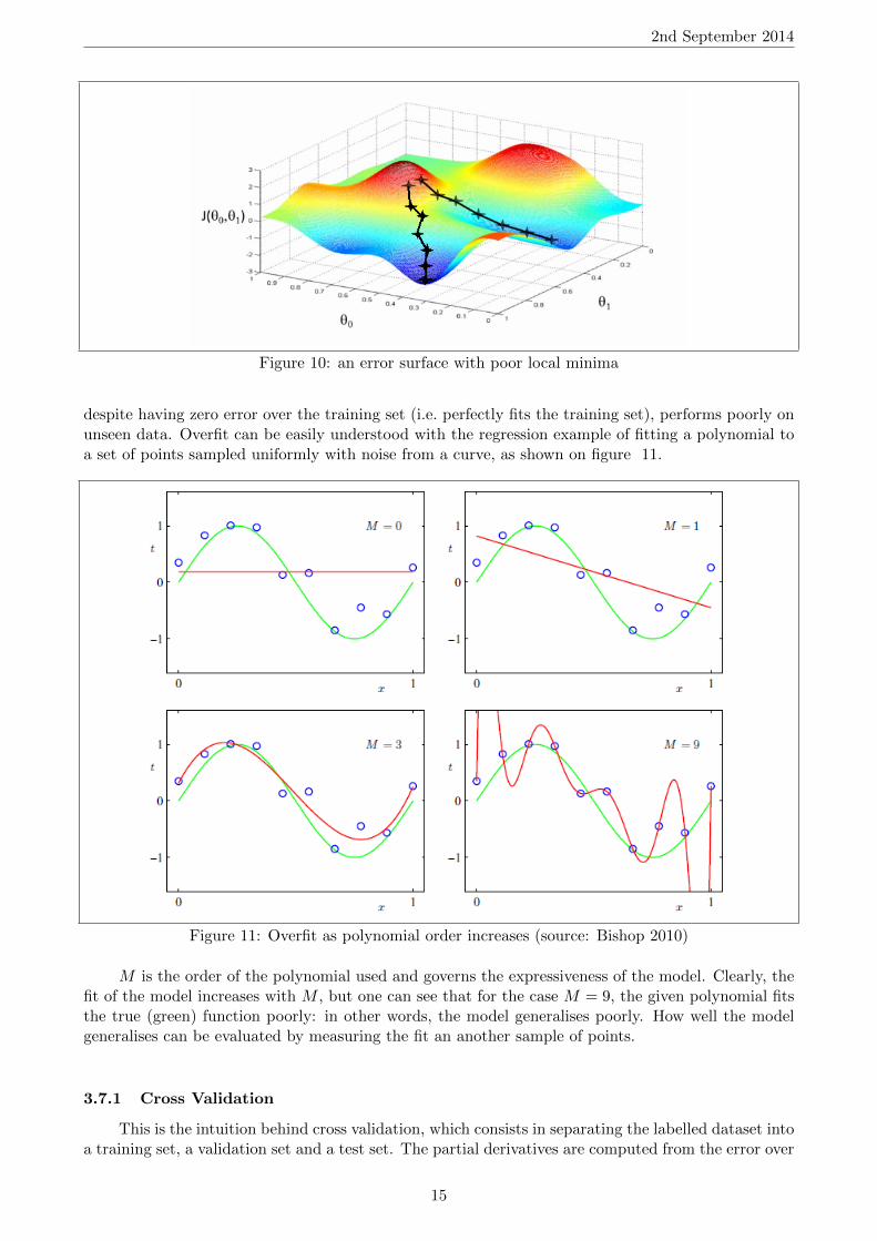
Visually, this means that weight values move in the direction that will (locally) reduce the errorquickest, i.e. the direction of steepest (local) descent on the error surface is taken. Notice that giventhe learning rule, gradient descent converges (i.e. wi,t+1 equals wi,t+1) when the partial derivativereaches zero. This corresponds to a local minimum on the error surface. In figure 10, two trainingsessions are illustrated: the only difference is the initialisation of the (two) weights, and the minimaattained in each case are not the same. This illustrates a strong shortcoming with backpropagation:parameter values can get stuck in poor local minima.

3.6.3 Stochastic Gradient Descent

In practice, in order to ensure use precise weight updates, the partial derivatives are obtained byaveraging over a number of training cases (which are often said to be grouped in ‘mini batches’). Thisis called Stochastic Gradient Descent [17], and is also referred to as ‘mini batch training’.

3.7 Overfit

As mentioned previously, learning is not a mere approximation problem because the hypothesisfunction must generalise well to any subset of the instance space. A downside to using highly expressivemodels such as deep neural networks is the danger of overfit: training may converge to a function that,

1the bound on weight perturbations is no longer tight if we drop the assumption of fully connected layers

14

2nd September 2014

Figure 10: an error surface with poor local minima

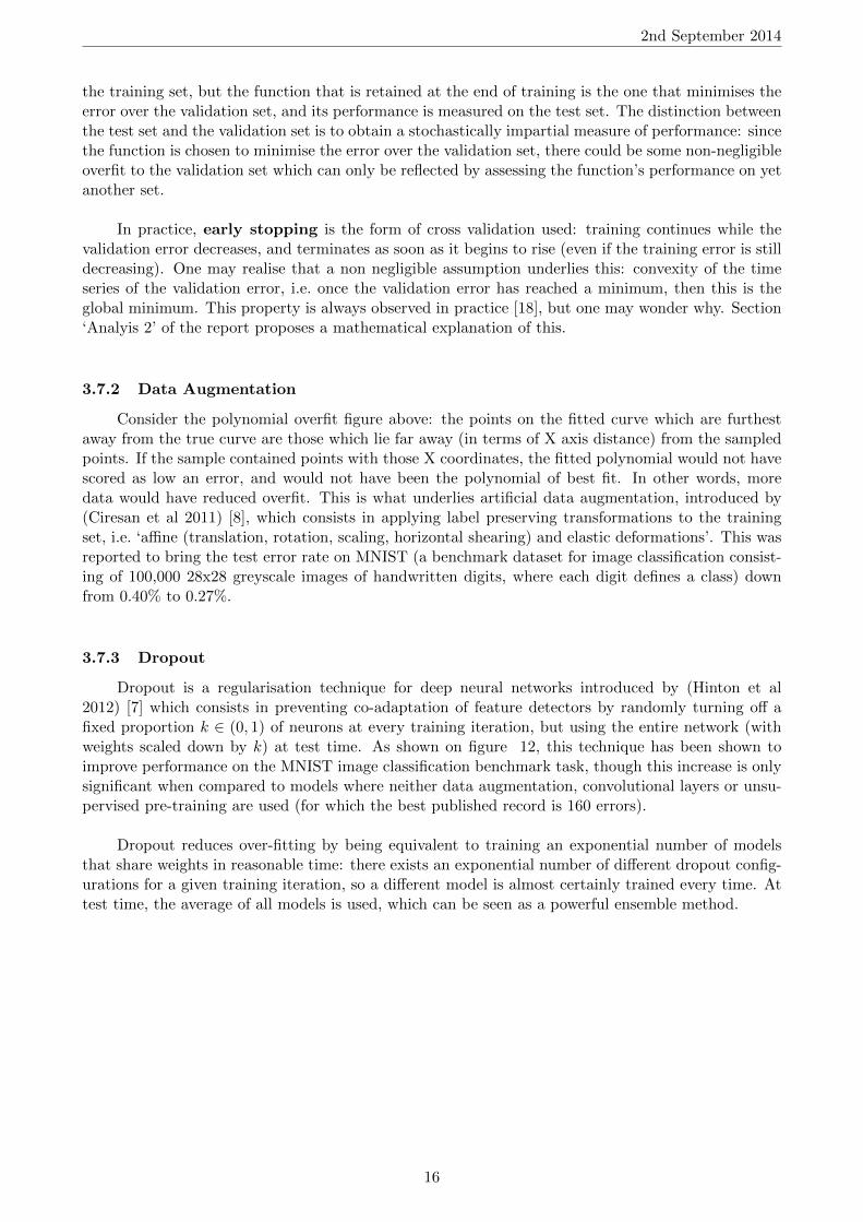
despite having zero error over the training set (i.e. perfectly fits the training set), performs poorly onunseen data. Overfit can be easily understood with the regression example of fitting a polynomial toa set of points sampled uniformly with noise from a curve, as shown on figure 11.

Figure 11: Overfit as polynomial order increases (source: Bishop 2010)

M is the order of the polynomial used and governs the expressiveness of the model. Clearly, thefit of the model increases with M , but one can see that for the case M = 9, the given polynomial fitsthe true (green) function poorly: in other words, the model generalises poorly. How well the modelgeneralises can be evaluated by measuring the fit an another sample of points.

3.7.1 Cross Validation

This is the intuition behind cross validation, which consists in separating the labelled dataset intoa training set, a validation set and a test set. The partial derivatives are computed from the error over

15

2nd September 2014

the training set, but the function that is retained at the end of training is the one that minimises theerror over the validation set, and its performance is measured on the test set. The distinction betweenthe test set and the validation set is to obtain a stochastically impartial measure of performance: sincethe function is chosen to minimise the error over the validation set, there could be some non-negligibleoverfit to the validation set which can only be reflected by assessing the function’s performance on yetanother set.

In practice, early stopping is the form of cross validation used: training continues while thevalidation error decreases, and terminates as soon as it begins to rise (even if the training error is stilldecreasing). One may realise that a non negligible assumption underlies this: convexity of the timeseries of the validation error, i.e. once the validation error has reached a minimum, then this is theglobal minimum. This property is always observed in practice [18], but one may wonder why. Section‘Analyis 2’ of the report proposes a mathematical explanation of this.

3.7.2 Data Augmentation

Consider the polynomial overfit figure above: the points on the fitted curve which are furthestaway from the true curve are those which lie far away (in terms of X axis distance) from the sampledpoints. If the sample contained points with those X coordinates, the fitted polynomial would not havescored as low an error, and would not have been the polynomial of best fit. In other words, moredata would have reduced overfit. This is what underlies artificial data augmentation, introduced by(Ciresan et al 2011) [8], which consists in applying label preserving transformations to the trainingset, i.e. ‘affine (translation, rotation, scaling, horizontal shearing) and elastic deformations’. This wasreported to bring the test error rate on MNIST (a benchmark dataset for image classification consist-ing of 100,000 28x28 greyscale images of handwritten digits, where each digit defines a class) downfrom 0.40% to 0.27%.

3.7.3 Dropout

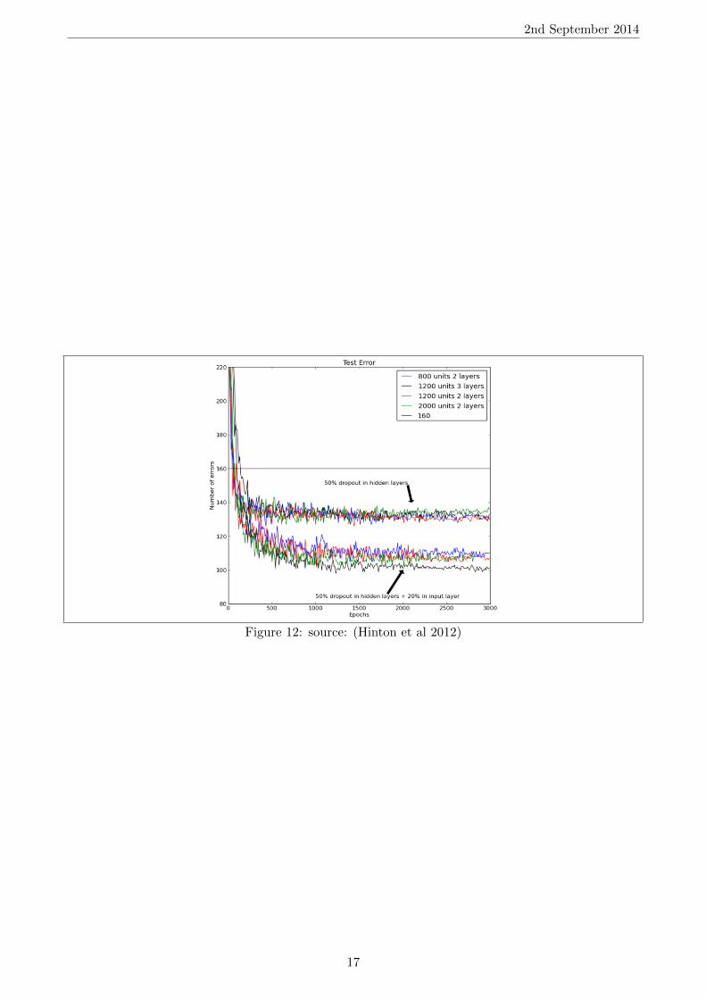
Dropout is a regularisation technique for deep neural networks introduced by (Hinton et al2012) [7] which consists in preventing co-adaptation of feature detectors by randomly turning off afixed proportion k ∈ (0, 1) of neurons at every training iteration, but using the entire network (withweights scaled down by k) at test time. As shown on figure 12, this technique has been shown toimprove performance on the MNIST image classification benchmark task, though this increase is onlysignificant when compared to models where neither data augmentation, convolutional layers or unsu-pervised pre-training are used (for which the best published record is 160 errors).

Dropout reduces over-fitting by being equivalent to training an exponential number of modelsthat share weights in reasonable time: there exists an exponential number of different dropout config-urations for a given training iteration, so a different model is almost certainly trained every time. Attest time, the average of all models is used, which can be seen as a powerful ensemble method.

16

2nd September 2014

Figure 12: source: (Hinton et al 2012)

17

2nd September 2014

3.8 Deep Convolutional Neural Networks

A convolutional neural network is a deep feed-forward neural network with at least one convolu-tional layer. A convolutional layer differs from a traditional fully connected layer in that it imposesspecific operations on the data before and after the data is fed through the activation functions. Thesespecific operations are taken from the pre deep learning era of computer vision, and are detailed inthis subsection.

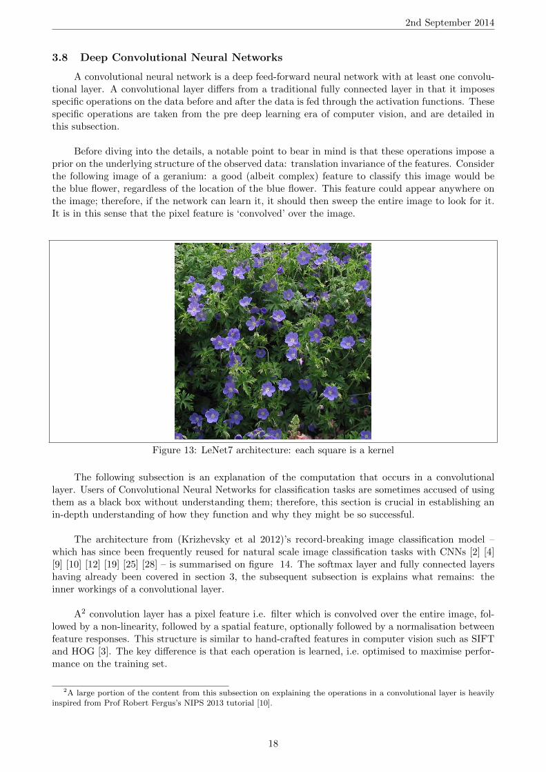
Before diving into the details, a notable point to bear in mind is that these operations impose aprior on the underlying structure of the observed data: translation invariance of the features. Considerthe following image of a geranium: a good (albeit complex) feature to classify this image would bethe blue flower, regardless of the location of the blue flower. This feature could appear anywhere onthe image; therefore, if the network can learn it, it should then sweep the entire image to look for it.It is in this sense that the pixel feature is ‘convolved’ over the image.

Figure 13: LeNet7 architecture: each square is a kernel

The following subsection is an explanation of the computation that occurs in a convolutionallayer. Users of Convolutional Neural Networks for classification tasks are sometimes accused of usingthem as a black box without understanding them; therefore, this section is crucial in establishing anin-depth understanding of how they function and why they might be so successful.

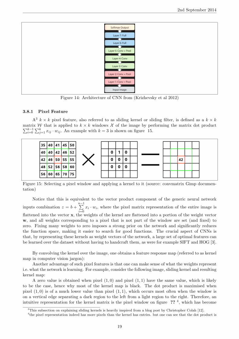
The architecture from (Krizhevsky et al 2012)’s record-breaking image classification model –which has since been frequently reused for natural scale image classification tasks with CNNs [2] [4][9] [10] [12] [19] [25] [28] – is summarised on figure 14. The softmax layer and fully connected layershaving already been covered in section 3, the subsequent subsection is explains what remains: theinner workings of a convolutional layer.

A2 convolution layer has a pixel feature i.e. filter which is convolved over the entire image, fol-lowed by a non-linearity, followed by a spatial feature, optionally followed by a normalisation betweenfeature responses. This structure is similar to hand-crafted features in computer vision such as SIFTand HOG [3]. The key difference is that each operation is learned, i.e. optimised to maximise perfor-mance on the training set.

2A large portion of the content from this subsection on explaining the operations in a convolutional layer is heavilyinspired from Prof Robert Fergus’s NIPS 2013 tutorial [10].

18

2nd September 2014

Figure 14: Architecture of CNN from (Krizhevsky et al 2012)

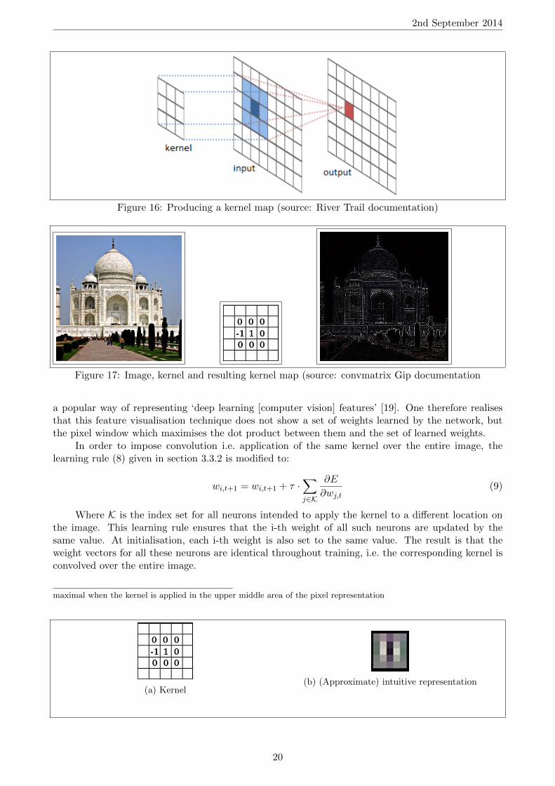
3.8.1 Pixel Feature

A3 k × k pixel feature, also referred to as sliding kernel or sliding filter, is defined as a k × kmatrix W that is applied to k × k windows X of the image by performing the matrix dot product∑k−1

i=0

∑kj=1 xij · wij . An example with k = 3 is shown on figure 15.

Figure 15: Selecting a pixel window and applying a kernel to it (source: convmatrix Gimp documen-tation)

Notice that this is equivalent to the vector product component of the generic neural network

inputs combination z = b +n−1∑i=0

xi · wi, where the pixel matrix representation of the entire image is

flattened into the vector x, the weights of the kernel are flattened into a portion of the weight vectorw, and all weights corresponding to a pixel that is not part of the window are set (and fixed) tozero. Fixing many weights to zero imposes a strong prior on the network and significantly reducesthe function space, making it easier to search for good functions. The crucial aspect of CNNs isthat, by representing these kernels as weight vectors of the network, a large set of optimal features canbe learned over the dataset without having to handcraft them, as were for example SIFT and HOG [3].

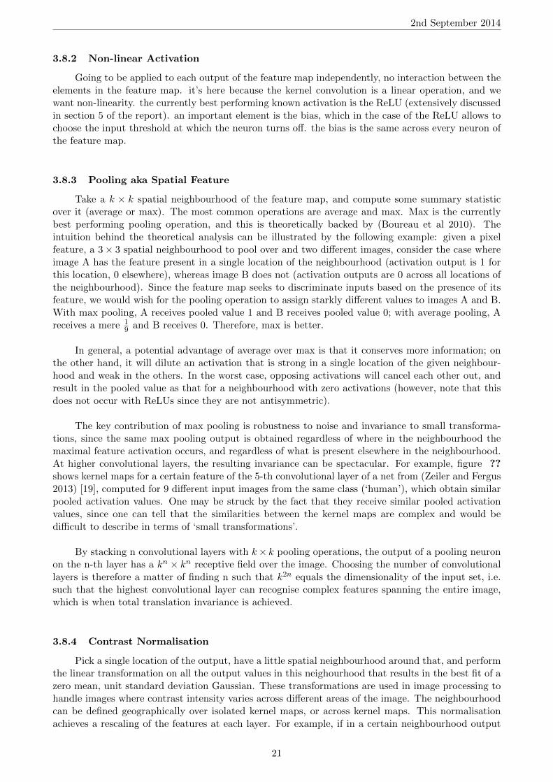
By convolving the kernel over the image, one obtains a feature response map (referred to as kernelmap in computer vision jargon):

Another advantage of such pixel features is that one can make sense of what the weights representi.e. what the network is learning. For example, consider the following image, sliding kernel and resultingkernel map:

A zero value is obtained when pixel (1, 0) and pixel (1, 1) have the same value, which is likelyto be the case, hence why most of the kernel map is black. The dot product is maximised whenpixel (1, 0) is of a much lower value than pixel (1, 1), which occurs most often when the window ison a vertical edge separating a dark region to the left from a light region to the right. Therefore, anintuitive representation for the kernel matrix is the pixel window on figure ?? 4, which has become

3This subsection on explaining sliding kernels is heavily inspired from a blog post by Christopher Colah [12].4the pixel representation indeed has more pixels than the kernel has entries. but one can see that the dot product is

19

2nd September 2014

Figure 16: Producing a kernel map (source: River Trail documentation)

Figure 17: Image, kernel and resulting kernel map (source: convmatrix Gip documentation

a popular way of representing ‘deep learning [computer vision] features’ [19]. One therefore realisesthat this feature visualisation technique does not show a set of weights learned by the network, butthe pixel window which maximises the dot product between them and the set of learned weights.

In order to impose convolution i.e. application of the same kernel over the entire image, thelearning rule (8) given in section 3.3.2 is modified to:

wi,t+1 = wi,t+1 + τ ·∑j∈K

∂E

∂wj,t(9)

Where K is the index set for all neurons intended to apply the kernel to a different location onthe image. This learning rule ensures that the i-th weight of all such neurons are updated by thesame value. At initialisation, each i-th weight is also set to the same value. The result is that theweight vectors for all these neurons are identical throughout training, i.e. the corresponding kernel isconvolved over the entire image.

maximal when the kernel is applied in the upper middle area of the pixel representation

(a) Kernel(b) (Approximate) intuitive representation

20

2nd September 2014

3.8.2 Non-linear Activation

Going to be applied to each output of the feature map independently, no interaction between theelements in the feature map. it’s here because the kernel convolution is a linear operation, and wewant non-linearity. the currently best performing known activation is the ReLU (extensively discussedin section 5 of the report). an important element is the bias, which in the case of the ReLU allows tochoose the input threshold at which the neuron turns off. the bias is the same across every neuron ofthe feature map.

3.8.3 Pooling aka Spatial Feature

Take a k × k spatial neighbourhood of the feature map, and compute some summary statisticover it (average or max). The most common operations are average and max. Max is the currentlybest performing pooling operation, and this is theoretically backed by (Boureau et al 2010). Theintuition behind the theoretical analysis can be illustrated by the following example: given a pixelfeature, a 3× 3 spatial neighbourhood to pool over and two different images, consider the case whereimage A has the feature present in a single location of the neighbourhood (activation output is 1 forthis location, 0 elsewhere), whereas image B does not (activation outputs are 0 across all locations ofthe neighbourhood). Since the feature map seeks to discriminate inputs based on the presence of itsfeature, we would wish for the pooling operation to assign starkly different values to images A and B.With max pooling, A receives pooled value 1 and B receives pooled value 0; with average pooling, Areceives a mere 1

9 and B receives 0. Therefore, max is better.

In general, a potential advantage of average over max is that it conserves more information; onthe other hand, it will dilute an activation that is strong in a single location of the given neighbour-hood and weak in the others. In the worst case, opposing activations will cancel each other out, andresult in the pooled value as that for a neighbourhood with zero activations (however, note that thisdoes not occur with ReLUs since they are not antisymmetric).

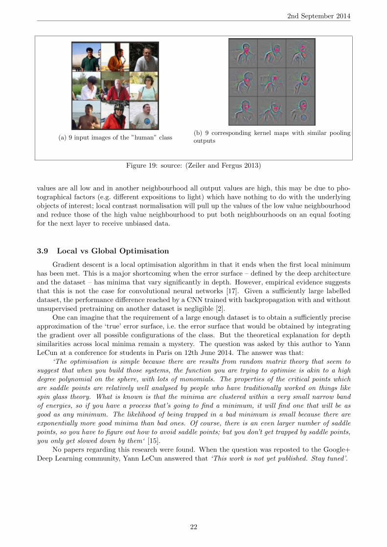
The key contribution of max pooling is robustness to noise and invariance to small transforma-tions, since the same max pooling output is obtained regardless of where in the neighbourhood themaximal feature activation occurs, and regardless of what is present elsewhere in the neighbourhood.At higher convolutional layers, the resulting invariance can be spectacular. For example, figure ??shows kernel maps for a certain feature of the 5-th convolutional layer of a net from (Zeiler and Fergus2013) [19], computed for 9 different input images from the same class (‘human’), which obtain similarpooled activation values. One may be struck by the fact that they receive similar pooled activationvalues, since one can tell that the similarities between the kernel maps are complex and would bedifficult to describe in terms of ‘small transformations’.

By stacking n convolutional layers with k× k pooling operations, the output of a pooling neuronon the n-th layer has a kn × kn receptive field over the image. Choosing the number of convolutionallayers is therefore a matter of finding n such that k2n equals the dimensionality of the input set, i.e.such that the highest convolutional layer can recognise complex features spanning the entire image,which is when total translation invariance is achieved.

3.8.4 Contrast Normalisation

Pick a single location of the output, have a little spatial neighbourhood around that, and performthe linear transformation on all the output values in this neighourhood that results in the best fit of azero mean, unit standard deviation Gaussian. These transformations are used in image processing tohandle images where contrast intensity varies across different areas of the image. The neighbourhoodcan be defined geographically over isolated kernel maps, or across kernel maps. This normalisationachieves a rescaling of the features at each layer. For example, if in a certain neighbourhood output

21

2nd September 2014

(a) 9 input images of the ”human” class(b) 9 corresponding kernel maps with similar poolingoutputs

Figure 19: source: (Zeiler and Fergus 2013)

values are all low and in another neighbourhood all output values are high, this may be due to pho-tographical factors (e.g. different expositions to light) which have nothing to do with the underlyingobjects of interest; local contrast normalisation will pull up the values of the low value neighbourhoodand reduce those of the high value neighbourhood to put both neighbourhoods on an equal footingfor the next layer to receive unbiased data.

3.9 Local vs Global Optimisation

Gradient descent is a local optimisation algorithm in that it ends when the first local minimumhas been met. This is a major shortcoming when the error surface – defined by the deep architectureand the dataset – has minima that vary significantly in depth. However, empirical evidence suggeststhat this is not the case for convolutional neural networks [17]. Given a sufficiently large labelleddataset, the performance difference reached by a CNN trained with backpropagation with and withoutunsupervised pretraining on another dataset is negligible [2].

One can imagine that the requirement of a large enough dataset is to obtain a sufficiently preciseapproximation of the ‘true’ error surface, i.e. the error surface that would be obtained by integratingthe gradient over all possible configurations of the class. But the theoretical explanation for depthsimilarities across local minima remain a mystery. The question was asked by this author to YannLeCun at a conference for students in Paris on 12th June 2014. The answer was that:

‘The optimisation is simple because there are results from random matrix theory that seem tosuggest that when you build those systems, the function you are trying to optimise is akin to a highdegree polynomial on the sphere, with lots of monomials. The properties of the critical points whichare saddle points are relatively well analysed by people who have traditionally worked on things likespin glass theory. What is known is that the minima are clustered within a very small narrow bandof energies, so if you have a process that’s going to find a minimum, it will find one that will be asgood as any minimum. The likelihood of being trapped in a bad minimum is small because there areexponentially more good minima than bad ones. Of course, there is an even larger number of saddlepoints, so you have to figure out how to avoid saddle points; but you don’t get trapped by saddle points,you only get slowed down by them‘ [15].

No papers regarding this research were found. When the question was reposted to the Google+Deep Learning community, Yann LeCun answered that ‘This work is not yet published. Stay tuned’.

22

2nd September 2014

The objective of the literature review until now has been to serve as a preamble, in order tounderstand the models which were used throughout the project. The two subsections that follow aremore specific and relate to challenges encountered when training classifiers for ControlPoint. Thepapers discussed were read in an ad hoc manner, so their relevance will become clearer later on in theExperiments sections that bear the same name. Therefore, especially in the case of the class imbalanceliterature, deeper examination of the papers is left for then.

3.10 Transfer Learning

Transfer learning consists in initialising the weights of layers of a network to those of dimen-sionally identical layers of a network trained in a supervised fashion on a similar task. Until 2013,the established approach consisted in transferring the weights of a Deep Belief Net trained (in anunsupervised fashion) on a ‘source’ unlabelled dataset [27]. However, the 2014 paper ”CNN Featuresoff-the-shelf: an Astounding Baseline for Recognition” by Razavian et al shows that transferring theweights of OverFeat – a model that is identical to AlexNet in architecture and winner of the ILSVRC2013 challenge [25] – to initialise the training of classifiers on 11 well known computer vision recognitiontasks, establishes state-of-the-art results on 10 of them [11].

The transfer models are obtained by training linear Support Vector Machines on the feature spacedefined by the bottom seven layers of OverFeat. The subsection below is therefore a rapid overviewof the mathematics that underlie the training of a linear SVM.

3.10.1 Linear Support Vector Machines

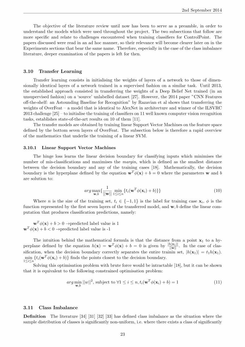
The hinge loss learns the linear decision boundary for classifying inputs which minimises thenumber of mis-classifications and maximises the margin, which is defined as the smallest distancebetween the decision boundary and any of the training cases [18]. Mathematically, the decisionboundary is the hyperplane defined by the equation wTφ(x) + b = 0 where the parameters w and bare solution to:

argmaxw,b 1

||w||min

1≤i≤nti(wTφ(xi) + b) (10)

Where n is the size of the training set, ti ∈ −1, 1 is the label for training case xi, φ is thefunction represented by the first seven layers of the transferred model, and w, b define the linear com-putation that produces classification predictions, namely:

wTφ(x) + b > 0→predicted label value is 1wTφ(x) + b < 0→predicted label value is -1

The intuition behind the mathematical formula is that the distance from a point x1 to a hy-perplane defined by the equation h(x) = wTφ(x) + b = 0 is given by |h(x1)|

||w|| . In the case of clas-

sification, when the decision boundary correctly separates the entire trainin set, |h(x1)| = t1h(x1).min

1≤i≤nti(wTφ(xi) + b) finds the points closest to the decision boundary.

Solving this optimisation problem with brute force would be intractable [18], but it can be shownthat it is equivalent to the following constrained optimisation problem:

argminw,b||w||2, subject to ∀1 ≤ i ≤ n, ti(wTφ(xi) + b) = 1 (11)

3.11 Class Imbalance

Definition The literature [34] [31] [32] [33] has defined class imbalance as the situation where thesample distribution of classes is significantly non-uniform, i.e. where there exists a class of significantly

23

2nd September 2014

smaller size than another. However, as will be seen later, this definition does not necessarily makeclass imbalance detrimental to learning. A definition for ‘dangerous class imbalance’ will be given withthe aim of being the largest set of conditions that are necessary for class imbalance to be detrimentalto training classifiers with stochastic gradient descent and standard cost functions.

The literature on deep learning with class imbalance was found to be scarce. Zhou and Liuin ‘Training cost sensitive neural networks with methods addressing the class imbalance problem’(2005) [32] experiment with under-sampling, textbfover-sampling and threshold-moving to dealwith class imbalance, and find threshold-moving to perform best.

‘F-measure as the error function to train neural networks’ by Pastor-Pellicer et al, 2013 [33],does not make use of these techniques and instead introduces a cost function for binary classifierswhich is the harmonic mean of precision and recall. Deep neural networks are trained on it as wellas on the Mean Squared Error for 3 image-cleaning tasks with levels of class imbalance below thoseexperimented with in this report. The image-cleaning task is framed as a classification task where theprobability of ink in each pixel of the clean image is to be predicted given the noisy image. MSE as acost function for training deep neural network classifiers is known to train slower and converge to thesame performance as when the cross entropy error is used [35].

The authors find that ‘both training techniques perform quite well’ on the basis that ‘a wellcleaned image gives good results on both metrics’. This seems to merely state that the error com-puted on a correctly classified input is low in absolute terms, for both cost functions. An analyticalcomparison of the cost functions by rescaling input domain and output range, such as the one betweensoftmax cross entropy and hinge loss in (Bishop 2010) [18] and in the previous section, is not included.An empirical comparison of the cost functions by evaluating a model trained on each against a com-mon performance metric such as percentage classification accuracy is not provided either. It appearsthat this cost function does not deliver significant performance gains.

24

2nd September 2014

(a) Activation functions

(b) source: Krizhevsky et al 2012

4 Analysis 1: ReLU Activation

4.1 Motivations

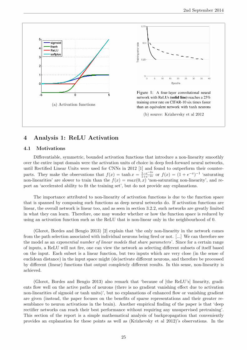
Differentiable, symmetric, bounded activation functions that introduce a non-linearity smoothlyover the entire input domain were the activation units of choice in deep feed-forward neural networks,until Rectified Linear Units were used for CNNs in 2012 [1] and found to outperform their counter-

parts. They make the observations that f(x) = tanhx = 1−e−2x

1+e−2x or f(x) = (1 + e−x)−1 ‘saturatingnon-linearities’ are slower to train than the f(x) = max(0, x) ‘non-saturating non-linearity’, and re-port an ‘accelerated ability to fit the training set’, but do not provide any explanations.

The importance attributed to non-linearity of activation functions is due to the function spacethat is spanned by composing such functions as deep neural networks do. If activation functions arelinear, the overall network is linear too, and as seen in section 3.2.2, such networks are greatly limitedin what they can learn. Therefore, one may wonder whether or how the function space is reduced byusing an activation function such as the ReLU that is non-linear only in the neighbourhood of 0.

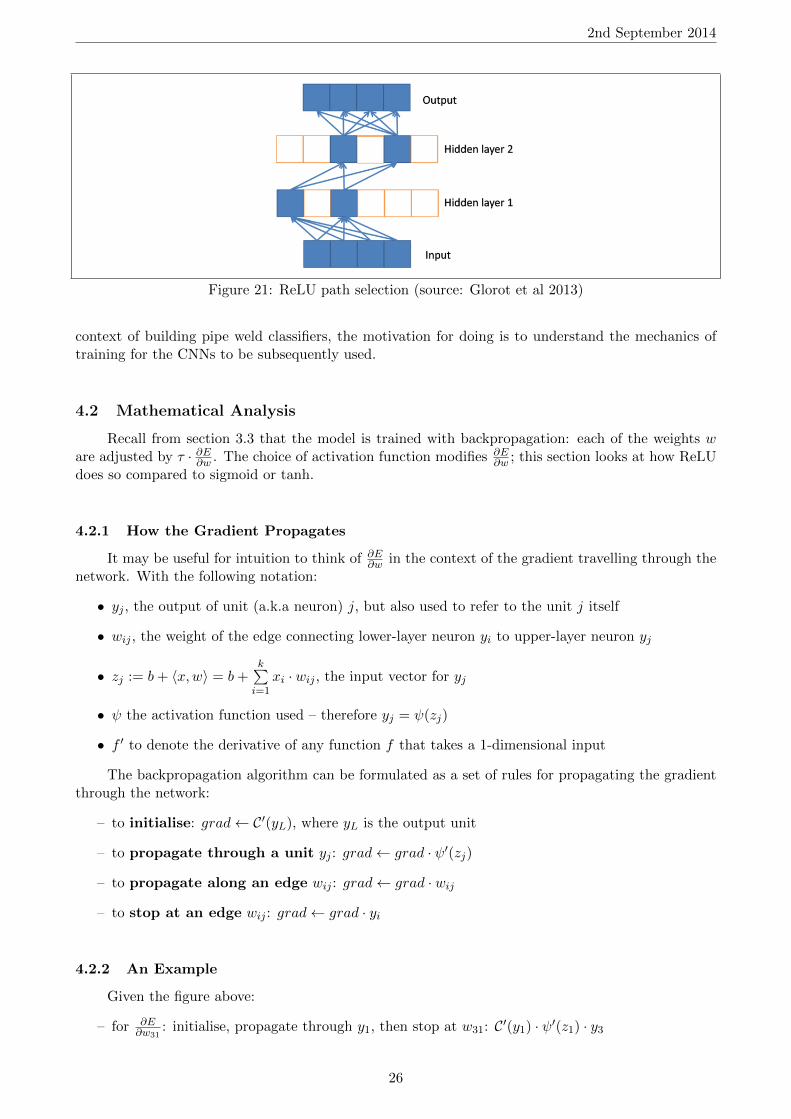
(Glorot, Bordes and Bengio 2013) [2] explain that ‘the only non-linearity in the network comesfrom the path selection associated with individual neurons being fired or not. [...] We can therefore seethe model as an exponential number of linear models that share parameters’. Since for a certain rangeof inputs, a ReLU will not fire, one can view the network as selecting different subsets of itself basedon the input. Each subset is a linear function, but two inputs which are very close (in the sense ofeuclidean distance) in the input space might (de)activate different neurons, and therefore be processedby different (linear) functions that output completely different results. In this sense, non-linearity isachieved.

(Glorot, Bordes and Bengio 2013) also remark that ‘because of [the ReLU’s] linearity, gradi-ents flow well on the active paths of neurons (there is no gradient vanishing effect due to activationnon-linearities of sigmoid or tanh units)’, but no explanations of enhanced flow or vanishing gradientare given (instead, the paper focuses on the benefits of sparse representations and their greater re-semblance to neuron activations in the brain). Another empirical finding of the paper is that ‘deeprectifier networks can reach their best performance without requiring any unsupervised pretraining’.This section of the report is a simple mathematical analysis of backpropagation that convenientlyprovides an explanation for these points as well as (Krizhevsky et al 2012)’s observations. In the

25

2nd September 2014

Figure 21: ReLU path selection (source: Glorot et al 2013)

context of building pipe weld classifiers, the motivation for doing is to understand the mechanics oftraining for the CNNs to be subsequently used.

4.2 Mathematical Analysis

Recall from section 3.3 that the model is trained with backpropagation: each of the weights ware adjusted by τ · ∂E∂w . The choice of activation function modifies ∂E

∂w ; this section looks at how ReLUdoes so compared to sigmoid or tanh.

4.2.1 How the Gradient Propagates

It may be useful for intuition to think of ∂E∂w in the context of the gradient travelling through the

network. With the following notation:

• yj , the output of unit (a.k.a neuron) j, but also used to refer to the unit j itself

• wij , the weight of the edge connecting lower-layer neuron yi to upper-layer neuron yj

• zj := b+ 〈x,w〉 = b+k∑

i=1xi · wij , the input vector for yj

• ψ the activation function used – therefore yj = ψ(zj)

• f ′ to denote the derivative of any function f that takes a 1-dimensional input

The backpropagation algorithm can be formulated as a set of rules for propagating the gradientthrough the network:

– to initialise: grad← C′(yL), where yL is the output unit

– to propagate through a unit yj : grad← grad · ψ′(zj)

– to propagate along an edge wij : grad← grad · wij

– to stop at an edge wij : grad← grad · yi

4.2.2 An Example

Given the figure above:

– for ∂E∂w31

: initialise, propagate through y1, then stop at w31: C′(y1) · ψ′(z1) · y3

26

2nd September 2014

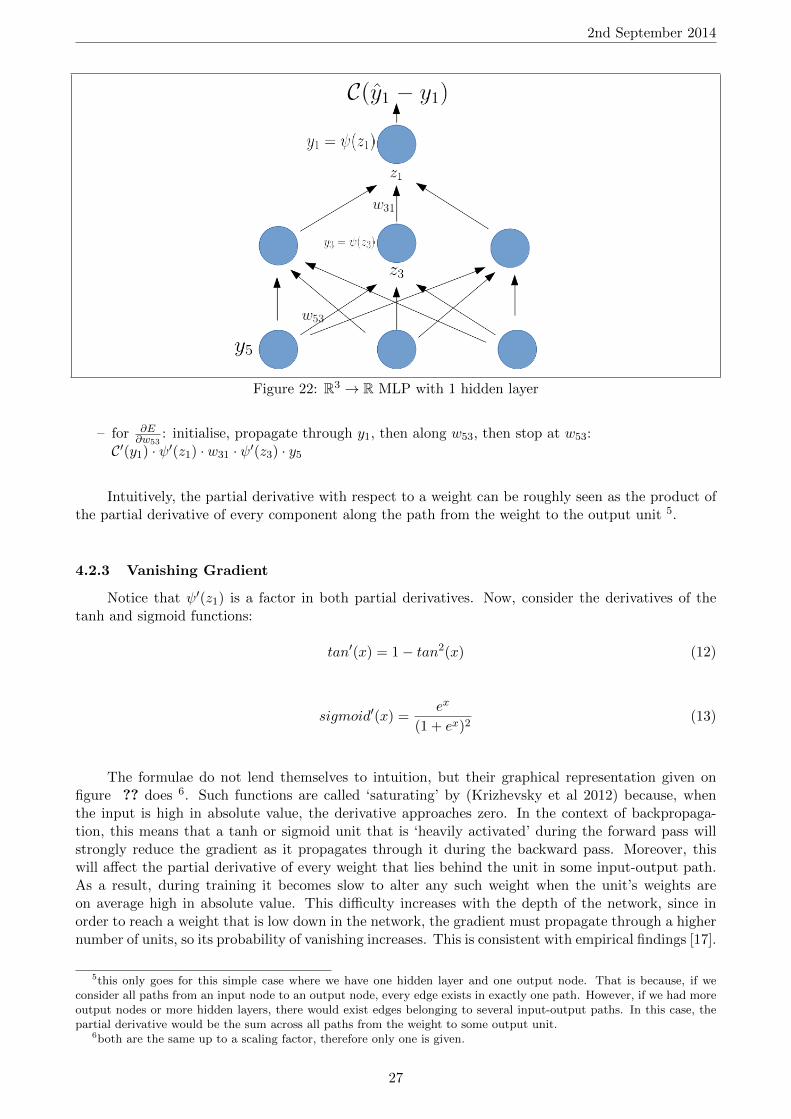
Figure 22: R3 → R MLP with 1 hidden layer

– for ∂E∂w53

: initialise, propagate through y1, then along w53, then stop at w53:C′(y1) · ψ′(z1) · w31 · ψ′(z3) · y5

Intuitively, the partial derivative with respect to a weight can be roughly seen as the product ofthe partial derivative of every component along the path from the weight to the output unit 5.

4.2.3 Vanishing Gradient

Notice that ψ′(z1) is a factor in both partial derivatives. Now, consider the derivatives of thetanh and sigmoid functions:

tan′(x) = 1− tan2(x) (12)

sigmoid′(x) =ex

(1 + ex)2(13)

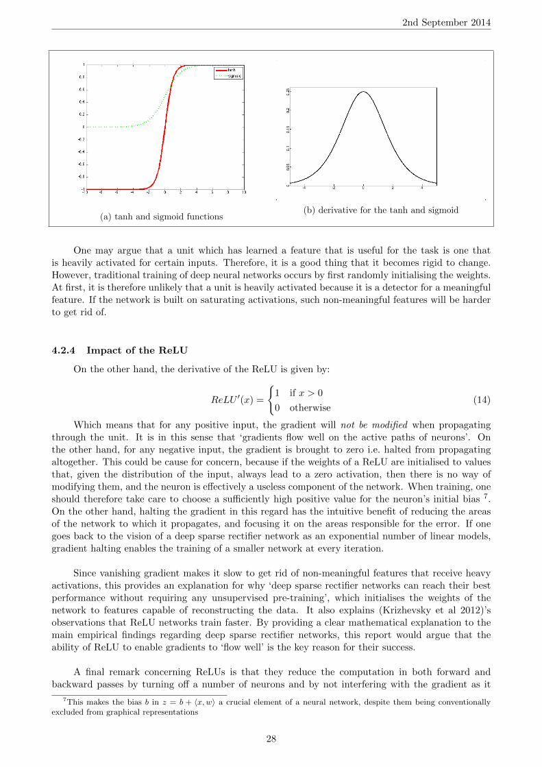
The formulae do not lend themselves to intuition, but their graphical representation given onfigure ?? does 6. Such functions are called ‘saturating’ by (Krizhevsky et al 2012) because, whenthe input is high in absolute value, the derivative approaches zero. In the context of backpropaga-tion, this means that a tanh or sigmoid unit that is ‘heavily activated’ during the forward pass willstrongly reduce the gradient as it propagates through it during the backward pass. Moreover, thiswill affect the partial derivative of every weight that lies behind the unit in some input-output path.As a result, during training it becomes slow to alter any such weight when the unit’s weights areon average high in absolute value. This difficulty increases with the depth of the network, since inorder to reach a weight that is low down in the network, the gradient must propagate through a highernumber of units, so its probability of vanishing increases. This is consistent with empirical findings [17].

5this only goes for this simple case where we have one hidden layer and one output node. That is because, if weconsider all paths from an input node to an output node, every edge exists in exactly one path. However, if we had moreoutput nodes or more hidden layers, there would exist edges belonging to several input-output paths. In this case, thepartial derivative would be the sum across all paths from the weight to some output unit.

6both are the same up to a scaling factor, therefore only one is given.

27

2nd September 2014

(a) tanh and sigmoid functions(b) derivative for the tanh and sigmoid

One may argue that a unit which has learned a feature that is useful for the task is one thatis heavily activated for certain inputs. Therefore, it is a good thing that it becomes rigid to change.However, traditional training of deep neural networks occurs by first randomly initialising the weights.At first, it is therefore unlikely that a unit is heavily activated because it is a detector for a meaningfulfeature. If the network is built on saturating activations, such non-meaningful features will be harderto get rid of.

4.2.4 Impact of the ReLU

On the other hand, the derivative of the ReLU is given by:

ReLU ′(x) =

1 if x > 0

0 otherwise(14)

Which means that for any positive input, the gradient will not be modified when propagatingthrough the unit. It is in this sense that ‘gradients flow well on the active paths of neurons’. Onthe other hand, for any negative input, the gradient is brought to zero i.e. halted from propagatingaltogether. This could be cause for concern, because if the weights of a ReLU are initialised to valuesthat, given the distribution of the input, always lead to a zero activation, then there is no way ofmodifying them, and the neuron is effectively a useless component of the network. When training, oneshould therefore take care to choose a sufficiently high positive value for the neuron’s initial bias 7.On the other hand, halting the gradient in this regard has the intuitive benefit of reducing the areasof the network to which it propagates, and focusing it on the areas responsible for the error. If onegoes back to the vision of a deep sparse rectifier network as an exponential number of linear models,gradient halting enables the training of a smaller network at every iteration.

Since vanishing gradient makes it slow to get rid of non-meaningful features that receive heavyactivations, this provides an explanation for why ‘deep sparse rectifier networks can reach their bestperformance without requiring any unsupervised pre-training’, which initialises the weights of thenetwork to features capable of reconstructing the data. It also explains (Krizhevsky et al 2012)’sobservations that ReLU networks train faster. By providing a clear mathematical explanation to themain empirical findings regarding deep sparse rectifier networks, this report would argue that theability of ReLU to enable gradients to ‘flow well’ is the key reason for their success.

A final remark concerning ReLUs is that they reduce the computation in both forward andbackward passes by turning off a number of neurons and by not interfering with the gradient as it

7This makes the bias b in z = b + 〈x,w〉 a crucial element of a neural network, despite them being conventionallyexcluded from graphical representations

28

2nd September 2014

propagates through a unit.

29

2nd September 2014

5 Experiments 1: Identifying Class Imbalance

5.1 Implementation: Cuda-Convnet

Due to its success and frequent re-use [2] [4] [9] [10] [12] [19] [25] [28], the network architecturefrom (Krizhevsky et al 2012), often referred to as AlexNet, was chosen for this task (and throughoutmost of the project).

Cuda-Convnet is an open-source GPU implementation for training deep convolutional neuralnetworks with stochastic gradient descent, written in CUDA C++ and python by Alex Krizhevsky.GPU implementations enable twenty-fold speedups [30] in training time. Knowledge of its use existedprior to this project since it had already been used for a group project. A shortcoming with the API isthat it expects data in the form of batches consisting of numpy arrays of stacked jpg values in matrixformat with RGB values split across, and a dictionary of labels and metadata. Python programs werewritten to achieve this and extract training data from the log files and plotting it. By re-using codewritten during the group project, the additional code needing to be written was limited to approx.400 lines. The hardware used for training the network was an nVidia GeForce GTX 780 with 4GBRAM, which enables a twenty-fold increase in training speed compared to the CPU.

5.2 Experimentation

Training occurred over the 113,865 image Redbox dataset only, to exclude domain change as apotential reason for weak performance if it were to occur. The task consists in learning three classes:‘No Clamps Used’, ‘Photo Does Not Show Enough Of Clamps’, and ‘Clamp Detected’ – which infact is the default class: an image belongs to it if none of the two mentioned flags have been raised.Time series for training and validation errors were extracted, but not the test error, since it serves nopurpose in training the model.

The error being computed and minimised by Cuda-Convnet is the negative of the log probabilityof the likelihood function:

− 1

n

n∑i=1

log(f(xi, li,W )) (15)

where f(xi, li,W ) is the model’s predicted probability for input xi’s label to be li, W are its param-eters, n is the mini-batch size. This is also known as Maximum Likelihood Estimation; thereforebackpropagation converges to the parameter values that maximise the joint likelihood of the trainingdata. It can be shown that this is equal to the cross entropy of the softmax layer’s output [17]. Thisis discussed in greater length in the experimentation section of Task 3 on class imbalance.

5.2.1 Non-Converging Error Rates

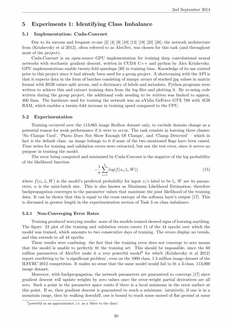
Training produced worrying results: none of the models trained showed signs of learning anything.The figure 24 plot of the training and validation errors covers 11 of the 44 epochs over which themodel was trained, which amounts to two consecutive days of training. The errors display no trends,and this extends to all 44 epochs.

These results were confusing: the fact that the training error does not converge to zero meansthat the model is unable to perfectly fit the training set. This should be impossible, since the 60million parameters of AlexNet make it a very powerful model8 for which (Krizhevsky et al 2012)report overfitting to be ‘a significant problem’, even on the 1000 class, 1.3 million image dataset of theILSVRC 2012 competition. It makes no sense that the same model would fail to fit a 3-class, 113,000image dataset.

Moreover, with backpropagation, the network parameters are guaranteed to converge [17] sincegradient descent will update weights by zero values once the error-weight partial derivatives are allzero. Such a point in the parameter space exists if there is a local minimum in the error surface atthis point. If so, then gradient descent is guaranteed to reach a minimum: intuitively, if one is in amountain range, then by walking downhill, one is bound to reach some morsel of flat ground at some

8powerful as an approximator, i.e. as a ‘fitter to the data’.

30

2nd September 2014

Figure 24: Test Run Training Results

point. Once the parameters have converged, the model is fixed, so its error is expected to be similaracross random samples of the training and validation sets. In this case, the persistent high amplitudeof the training and validation errors means that the error is heavily changing all the time.

A number of potential explanations for the high amplitude of the error rates were considered:

• The learning rates are too high: the minimum keeps getting ’overshot’, the weights move end-lessly around the rims of a bowl on the error surface9.

• The dropout rate is too high: since neurons are randomly dropped at every iteration, a differentmodel is tested every time. The errors correspond to partial derivatives of different models everytime, so the amplitude is high.

• The number of parameters is too high: AlexNet contains 60 million parameters, far more thanthan the number of training cases, so collinearities between the parameters cannot even bebroken, and most of them are rendered useless.

• The error rates are not computed correctly.

• Class imbalance: with 90% of the data belonging to the same class, there is not enough infor-mation about the ‘No Clamps Used’ and ‘Photo Does Not Show Enough of Clamps’ classes tobe able to learn features for them.

• Mislabelled data: the images were not tagged correctly, too many members of one class appearin the other and vice versa, so nothing can be learned.

The learning and dropout rates were modified to no avail. (Jarrett et al 2009) report successfultraining of networks for which ‘the number of parameters greatly outstrips the number of samples’.

5.2.2 Increase Validation Error Precision

If the set of images that the validation error is computed against varies from one iteration tothe next, then the variations in validation error are not solely explained by the changes in the modelparameters; they may also be due to changes in the validation set. Secondly, precision increases withthe size of the set. Therefore, by computing the validation error on a larger and unchanging sampleof images, one obtains stable, more precise measures that truly reflect what the model is learning.

9This interpretation was supported by the Google+ community when the plots were posted.

31

2nd September 2014

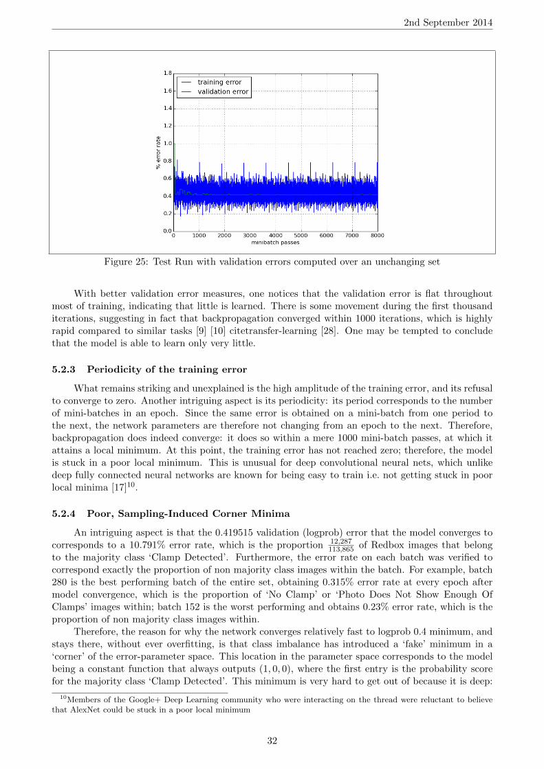
Figure 25: Test Run with validation errors computed over an unchanging set

With better validation error measures, one notices that the validation error is flat throughoutmost of training, indicating that little is learned. There is some movement during the first thousanditerations, suggesting in fact that backpropagation converged within 1000 iterations, which is highlyrapid compared to similar tasks [9] [10] citetransfer-learning [28]. One may be tempted to concludethat the model is able to learn only very little.

5.2.3 Periodicity of the training error

What remains striking and unexplained is the high amplitude of the training error, and its refusalto converge to zero. Another intriguing aspect is its periodicity: its period corresponds to the numberof mini-batches in an epoch. Since the same error is obtained on a mini-batch from one period tothe next, the network parameters are therefore not changing from an epoch to the next. Therefore,backpropagation does indeed converge: it does so within a mere 1000 mini-batch passes, at which itattains a local minimum. At this point, the training error has not reached zero; therefore, the modelis stuck in a poor local minimum. This is unusual for deep convolutional neural nets, which unlikedeep fully connected neural networks are known for being easy to train i.e. not getting stuck in poorlocal minima [17]10.

5.2.4 Poor, Sampling-Induced Corner Minima

An intriguing aspect is that the 0.419515 validation (logprob) error that the model converges tocorresponds to a 10.791% error rate, which is the proportion 12,287

113,865 of Redbox images that belongto the majority class ‘Clamp Detected’. Furthermore, the error rate on each batch was verified tocorrespond exactly the proportion of non majority class images within the batch. For example, batch280 is the best performing batch of the entire set, obtaining 0.315% error rate at every epoch aftermodel convergence, which is the proportion of ‘No Clamp’ or ‘Photo Does Not Show Enough OfClamps’ images within; batch 152 is the worst performing and obtains 0.23% error rate, which is theproportion of non majority class images within.

Therefore, the reason for why the network converges relatively fast to logprob 0.4 minimum, andstays there, without ever overfitting, is that class imbalance has introduced a ‘fake’ minimum in a‘corner’ of the error-parameter space. This location in the parameter space corresponds to the modelbeing a constant function that always outputs (1, 0, 0), where the first entry is the probability scorefor the majority class ‘Clamp Detected’. This minimum is very hard to get out of because it is deep:

10Members of the Google+ Deep Learning community who were interacting on the thread were reluctant to believethat AlexNet could be stuck in a poor local minimum

32

2nd September 2014

it enables the model to score a 10% error rate, which might be better than a number of other localminima. It is in ‘corner’ in the sense that it is far away from where the ‘real’ minima are because the‘real’ minima are in a region of the parameter space that corresponds to the network having learnedvisually meaningful features rather than being a constant function.

The high amplitude of the training error despite parameter convergence is therefore explained bythe variation in proportion of ‘Clamp Detected’ images across batches.

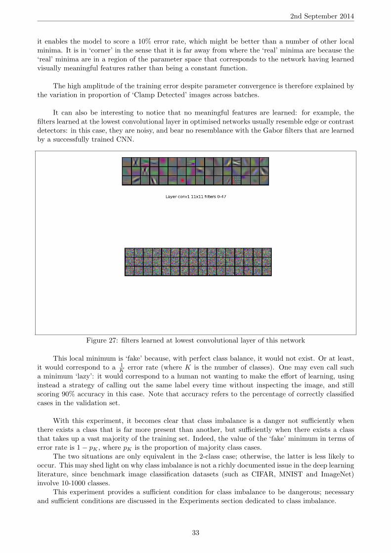
It can also be interesting to notice that no meaningful features are learned: for example, thefilters learned at the lowest convolutional layer in optimised networks usually resemble edge or contrastdetectors: in this case, they are noisy, and bear no resemblance with the Gabor filters that are learnedby a successfully trained CNN.

Figure 27: filters learned at lowest convolutional layer of this network

This local minimum is ‘fake’ because, with perfect class balance, it would not exist. Or at least,it would correspond to a 1

K error rate (where K is the number of classes). One may even call sucha minimum ‘lazy’: it would correspond to a human not wanting to make the effort of learning, usinginstead a strategy of calling out the same label every time without inspecting the image, and stillscoring 90% accuracy in this case. Note that accuracy refers to the percentage of correctly classifiedcases in the validation set.

With this experiment, it becomes clear that class imbalance is a danger not sufficiently whenthere exists a class that is far more present than another, but sufficiently when there exists a classthat takes up a vast majority of the training set. Indeed, the value of the ‘fake’ minimum in terms oferror rate is 1− pK , where pK is the proportion of majority class cases.

The two situations are only equivalent in the 2-class case; otherwise, the latter is less likely tooccur. This may shed light on why class imbalance is not a richly documented issue in the deep learningliterature, since benchmark image classification datasets (such as CIFAR, MNIST and ImageNet)involve 10-1000 classes.

This experiment provides a sufficient condition for class imbalance to be dangerous; necessaryand sufficient conditions are discussed in the Experiments section dedicated to class imbalance.

33

2nd September 2014

5.2.5 Mislabelling

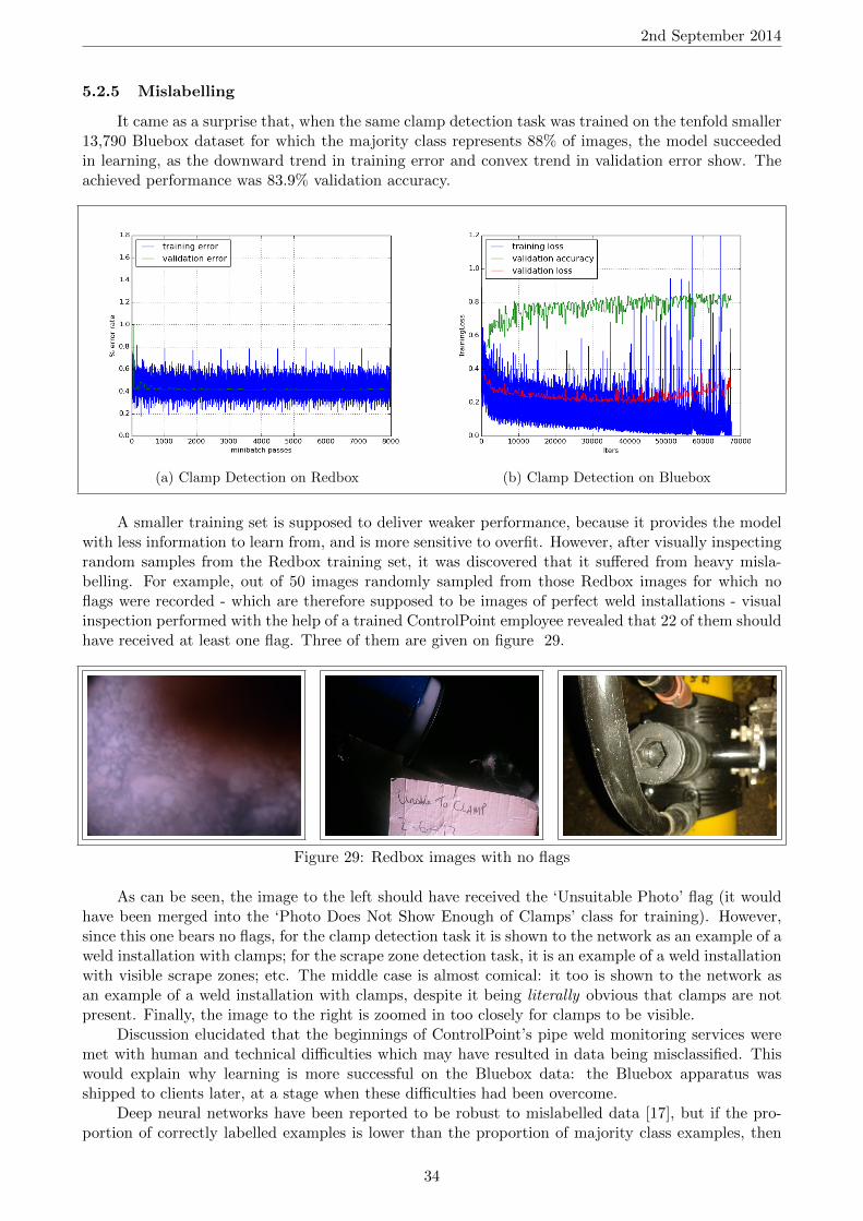
It came as a surprise that, when the same clamp detection task was trained on the tenfold smaller13,790 Bluebox dataset for which the majority class represents 88% of images, the model succeededin learning, as the downward trend in training error and convex trend in validation error show. Theachieved performance was 83.9% validation accuracy.

(a) Clamp Detection on Redbox (b) Clamp Detection on Bluebox

A smaller training set is supposed to deliver weaker performance, because it provides the modelwith less information to learn from, and is more sensitive to overfit. However, after visually inspectingrandom samples from the Redbox training set, it was discovered that it suffered from heavy misla-belling. For example, out of 50 images randomly sampled from those Redbox images for which noflags were recorded - which are therefore supposed to be images of perfect weld installations - visualinspection performed with the help of a trained ControlPoint employee revealed that 22 of them shouldhave received at least one flag. Three of them are given on figure 29.

Figure 29: Redbox images with no flags

As can be seen, the image to the left should have received the ‘Unsuitable Photo’ flag (it wouldhave been merged into the ‘Photo Does Not Show Enough of Clamps’ class for training). However,since this one bears no flags, for the clamp detection task it is shown to the network as an example of aweld installation with clamps; for the scrape zone detection task, it is an example of a weld installationwith visible scrape zones; etc. The middle case is almost comical: it too is shown to the network asan example of a weld installation with clamps, despite it being literally obvious that clamps are notpresent. Finally, the image to the right is zoomed in too closely for clamps to be visible.

Discussion elucidated that the beginnings of ControlPoint’s pipe weld monitoring services weremet with human and technical difficulties which may have resulted in data being misclassified. Thiswould explain why learning is more successful on the Bluebox data: the Bluebox apparatus wasshipped to clients later, at a stage when these difficulties had been overcome.

Deep neural networks have been reported to be robust to mislabelled data [17], but if the pro-portion of correctly labelled examples is lower than the proportion of majority class examples, then

34

2nd September 2014

bad minima are not just likely to occur, they are inevitable. Consider a hypothetical classifier withperfect understanding of the classes (e.g. a human expert from ControlPoint) which always assignsthe true label to any image, and a ‘lazy’ classifier which always assigns the majority class label to anyimage. Consider also a dataset with majority class proportion k and random assignment of incorrectclass labels to a proportion r of that dataset. The perfect classifier will obtain a 1 − r error rate,whereas the lazy classifier will obtain a k error rate. If r > 1− k then the lazy classifier will beat theperfect classifier. For clamp detection on the Redbox dataset, this is the case if more than 10.8% ofimages are missing a ‘No Clamps Used’ or a ‘Photo Does Not Show Enough Of Clamps’ flag. 8/50 ofthe randomly sampled flagless images were failed images akin to the unsuitable image shown above,and 4/50 were of the type shown in the middle or on the right. Since flagless images make up 43%of the training set, this estimate11 suggests that approximately 0.43 · 8+4

50 = 10.3% of Redbox imagesare mislabelled with regards to clamp detection. This would also imply that none of six other, lessfrequent flags can be learned using the Redbox dataset.

In order to limit the impact of mislabelling, the rest of the project was conducted solely with theuse of Bluebox data. This heavily reduced the amount of training data, motivating the use of transferlearning. It is worth noting that there is probably scope for making use of some of the Redbox databy exploring ways of filtering out some of mislabelled data; this is discussed in the conclusions of thereport. This path was not chosen because making use of transfer learning seemed to offer more focuson deep learning techniques than on characteristics specific to the datasets.

11One must concede that the estimate is imprecise due to the small size of the sample.

35

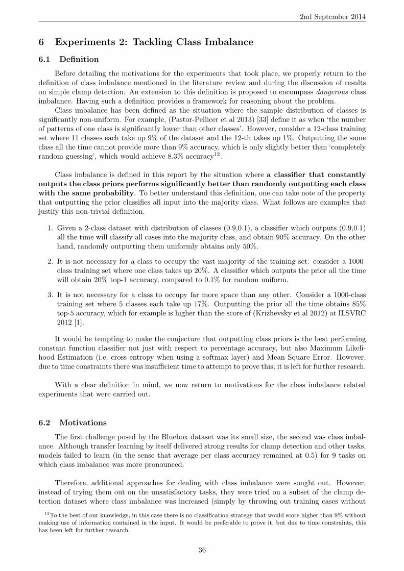
2nd September 2014

6 Experiments 2: Tackling Class Imbalance

6.1 Definition

Before detailing the motivations for the experiments that took place, we properly return to thedefinition of class imbalance mentioned in the literature review and during the discussion of resultson simple clamp detection. An extension to this definition is proposed to encompass dangerous classimbalance. Having such a definition provides a framework for reasoning about the problem.

Class imbalance has been defined as the situation where the sample distribution of classes issignificantly non-uniform. For example, (Pastor-Pellicer et al 2013) [33] define it as when ‘the numberof patterns of one class is significantly lower than other classes’. However, consider a 12-class trainingset where 11 classes each take up 9% of the dataset and the 12-th takes up 1%. Outputting the sameclass all the time cannot provide more than 9% accuracy, which is only slightly better than ‘completelyrandom guessing’, which would achieve 8.3% accuracy12.

Class imbalance is defined in this report by the situation where a classifier that constantlyoutputs the class priors performs significantly better than randomly outputting each classwith the same probability. To better understand this definition, one can take note of the propertythat outputting the prior classifies all input into the majority class. What follows are examples thatjustify this non-trivial definition.

1. Given a 2-class dataset with distribution of classes (0.9,0.1), a classifier which outputs (0.9,0.1)all the time will classify all cases into the majority class, and obtain 90% accuracy. On the otherhand, randomly outputting them uniformly obtains only 50%.

2. It is not necessary for a class to occupy the vast majority of the training set: consider a 1000-class training set where one class takes up 20%. A classifier which outputs the prior all the timewill obtain 20% top-1 accuracy, compared to 0.1% for random uniform.

3. It is not necessary for a class to occupy far more space than any other. Consider a 1000-classtraining set where 5 classes each take up 17%. Outputting the prior all the time obtains 85%top-5 accuracy, which for example is higher than the score of (Krizhevsky et al 2012) at ILSVRC2012 [1].

It would be tempting to make the conjecture that outputting class priors is the best performingconstant function classifier not just with respect to percentage accuracy, but also Maximum Likeli-hood Estimation (i.e. cross entropy when using a softmax layer) and Mean Square Error. However,due to time constraints there was insufficient time to attempt to prove this; it is left for further research.

With a clear definition in mind, we now return to motivations for the class imbalance relatedexperiments that were carried out.

6.2 Motivations

The first challenge posed by the Bluebox dataset was its small size, the second was class imbal-ance. Although transfer learning by itself delivered strong results for clamp detection and other tasks,models failed to learn (in the sense that average per class accuracy remained at 0.5) for 9 tasks onwhich class imbalance was more pronounced.

Therefore, additional approaches for dealing with class imbalance were sought out. However,instead of trying them out on the unsatisfactory tasks, they were tried on a subset of the clamp de-tection dataset where class imbalance was increased (simply by throwing out training cases without

12To the best of our knowledge, in this case there is no classification strategy that would score higher than 9% withoutmaking use of information contained in the input. It would be preferable to prove it, but due to time constraints, thishas been left for further research.

36

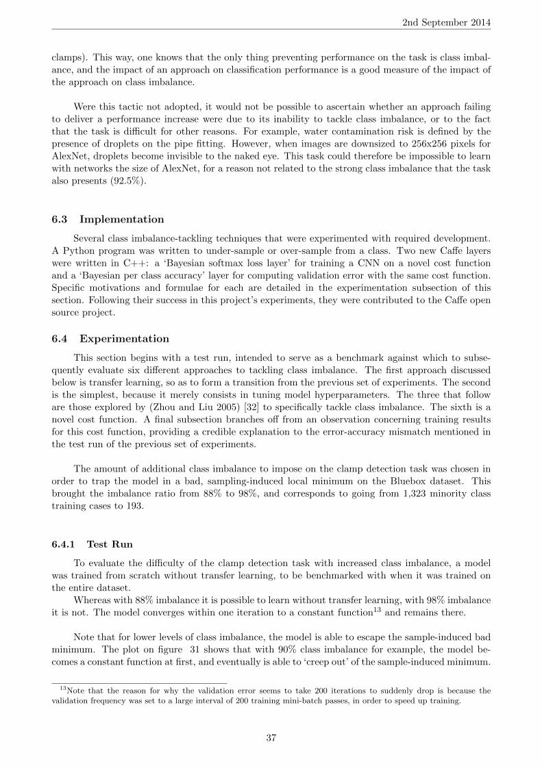
2nd September 2014

clamps). This way, one knows that the only thing preventing performance on the task is class imbal-ance, and the impact of an approach on classification performance is a good measure of the impact ofthe approach on class imbalance.

Were this tactic not adopted, it would not be possible to ascertain whether an approach failingto deliver a performance increase were due to its inability to tackle class imbalance, or to the factthat the task is difficult for other reasons. For example, water contamination risk is defined by thepresence of droplets on the pipe fitting. However, when images are downsized to 256x256 pixels forAlexNet, droplets become invisible to the naked eye. This task could therefore be impossible to learnwith networks the size of AlexNet, for a reason not related to the strong class imbalance that the taskalso presents (92.5%).

6.3 Implementation

Several class imbalance-tackling techniques that were experimented with required development.A Python program was written to under-sample or over-sample from a class. Two new Caffe layerswere written in C++: a ‘Bayesian softmax loss layer’ for training a CNN on a novel cost functionand a ‘Bayesian per class accuracy’ layer for computing validation error with the same cost function.Specific motivations and formulae for each are detailed in the experimentation subsection of thissection. Following their success in this project’s experiments, they were contributed to the Caffe opensource project.

6.4 Experimentation

This section begins with a test run, intended to serve as a benchmark against which to subse-quently evaluate six different approaches to tackling class imbalance. The first approach discussedbelow is transfer learning, so as to form a transition from the previous set of experiments. The secondis the simplest, because it merely consists in tuning model hyperparameters. The three that followare those explored by (Zhou and Liu 2005) [32] to specifically tackle class imbalance. The sixth is anovel cost function. A final subsection branches off from an observation concerning training resultsfor this cost function, providing a credible explanation to the error-accuracy mismatch mentioned inthe test run of the previous set of experiments.

The amount of additional class imbalance to impose on the clamp detection task was chosen inorder to trap the model in a bad, sampling-induced local minimum on the Bluebox dataset. Thisbrought the imbalance ratio from 88% to 98%, and corresponds to going from 1,323 minority classtraining cases to 193.

6.4.1 Test Run

To evaluate the difficulty of the clamp detection task with increased class imbalance, a modelwas trained from scratch without transfer learning, to be benchmarked with when it was trained onthe entire dataset.

Whereas with 88% imbalance it is possible to learn without transfer learning, with 98% imbalanceit is not. The model converges within one iteration to a constant function13 and remains there.

Note that for lower levels of class imbalance, the model is able to escape the sample-induced badminimum. The plot on figure 31 shows that with 90% class imbalance for example, the model be-comes a constant function at first, and eventually is able to ‘creep out’ of the sample-induced minimum.

13Note that the reason for why the validation error seems to take 200 iterations to suddenly drop is because thevalidation frequency was set to a large interval of 200 training mini-batch passes, in order to speed up training.

37

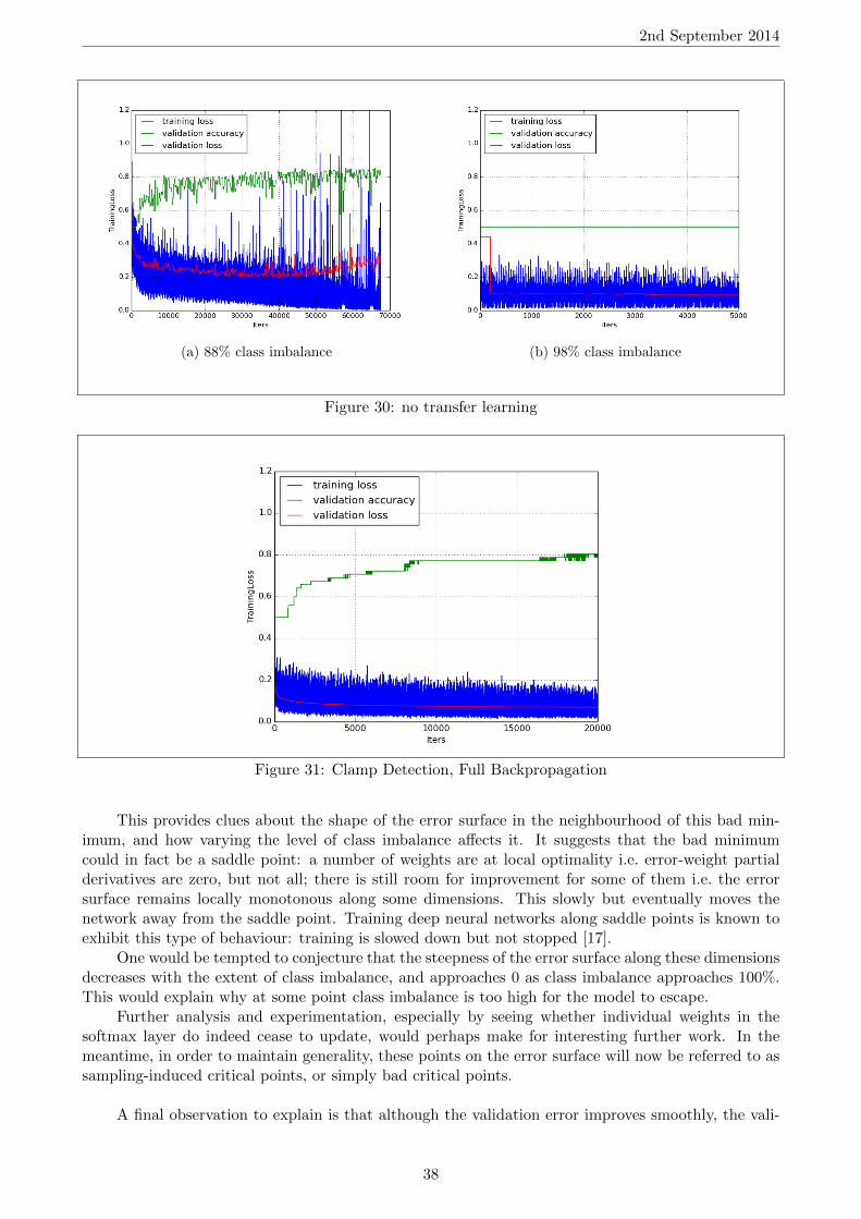
2nd September 2014

(a) 88% class imbalance (b) 98% class imbalance

Figure 30: no transfer learning

Figure 31: Clamp Detection, Full Backpropagation

This provides clues about the shape of the error surface in the neighbourhood of this bad min-imum, and how varying the level of class imbalance affects it. It suggests that the bad minimumcould in fact be a saddle point: a number of weights are at local optimality i.e. error-weight partialderivatives are zero, but not all; there is still room for improvement for some of them i.e. the errorsurface remains locally monotonous along some dimensions. This slowly but eventually moves thenetwork away from the saddle point. Training deep neural networks along saddle points is known toexhibit this type of behaviour: training is slowed down but not stopped [17].

One would be tempted to conjecture that the steepness of the error surface along these dimensionsdecreases with the extent of class imbalance, and approaches 0 as class imbalance approaches 100%.This would explain why at some point class imbalance is too high for the model to escape.

Further analysis and experimentation, especially by seeing whether individual weights in thesoftmax layer do indeed cease to update, would perhaps make for interesting further work. In themeantime, in order to maintain generality, these points on the error surface will now be referred to assampling-induced critical points, or simply bad critical points.

A final observation to explain is that although the validation error improves smoothly, the vali-

38

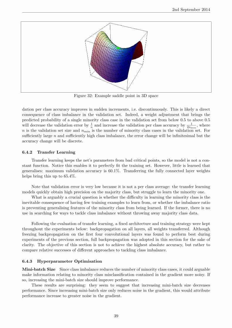
2nd September 2014

Figure 32: Example saddle point in 3D space

dation per class accuracy improves in sudden increments, i.e. discontinuously. This is likely a directconsequence of class imbalance in the validation set. Indeed, a weight adjustment that brings thepredicted probability of a single minority class case in the validation set from below 0.5 to above 0.5will decrease the validation error by 1

n and increase the validation per class accuracy by 12nmin

, wheren is the validation set size and nmin is the number of minority class cases in the validation set. Forsufficiently large n and sufficiently high class imbalance, the error change will be infinitesimal but theaccuracy change will be discrete.

6.4.2 Transfer Learning

Transfer learning keeps the net’s parameters from bad critical points, so the model is not a con-stant function. Notice this enables it to perfectly fit the training set. However, little is learned thatgeneralises: maximum validation accuracy is 60.1%. Transferring the fully connected layer weightshelps bring this up to 65.4%.

Note that validation error is very low because it is not a per class average: the transfer learningmodels quickly obtain high precision on the majority class, but struggle to learn the minority one.

What is arguably a crucial question is whether the difficulty in learning the minority class is theinevitable consequence of having few training examples to learn from, or whether the imbalance ratiois preventing generalising features of the minority class from being learned. If the former, there is nouse in searching for ways to tackle class imbalance without throwing away majority class data.

Following the evaluation of transfer learning, a fixed architecture and training strategy were keptthroughout the experiments below: backpropagation on all layers, all weights transferred. Althoughfreezing backpropagation on the first four convolutional layers was found to perform best duringexperiments of the previous section, full backpropagation was adopted in this section for the sake ofclarity. The objective of this section is not to achieve the highest absolute accuracy, but rather tocompare relative successes of different approaches to tackling class imbalance.

6.4.3 Hyperparameter Optimisation

Mini-batch Size Since class imbalance reduces the number of minority class cases, it could arguablemake information relating to minority class misclassification contained in the gradient more noisy. Ifso, increasing the mini-batch size should improve performance.

These results are surprising: they seem to suggest that increasing mini-batch size decreasesperformance. Since increasing mini-batch size only reduces noise in the gradient, this would attributeperformance increase to greater noise in the gradient.

39

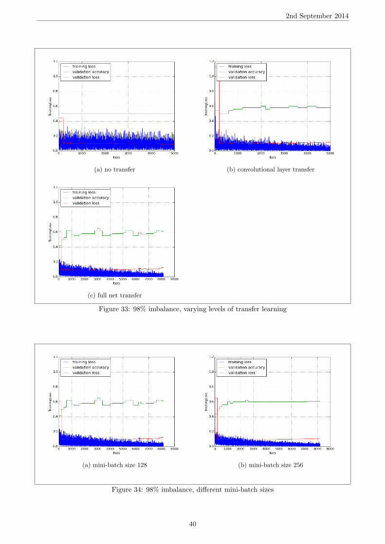
2nd September 2014

(a) no transfer (b) convolutional layer transfer

(c) full net transfer

Figure 33: 98% imbalance, varying levels of transfer learning

(a) mini-batch size 128 (b) mini-batch size 256

Figure 34: 98% imbalance, different mini-batch sizes

40

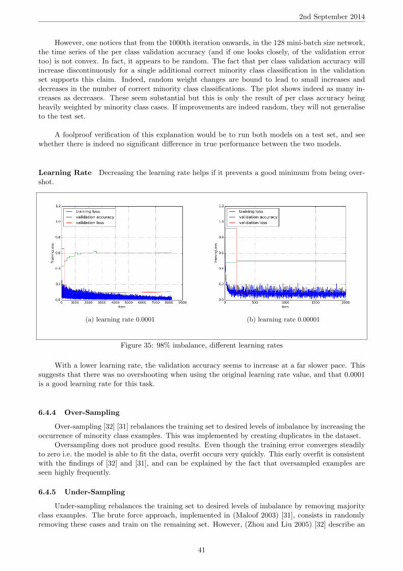
2nd September 2014

However, one notices that from the 1000th iteration onwards, in the 128 mini-batch size network,the time series of the per class validation accuracy (and if one looks closely, of the validation errortoo) is not convex. In fact, it appears to be random. The fact that per class validation accuracy willincrease discontinuously for a single additional correct minority class classification in the validationset supports this claim. Indeed, random weight changes are bound to lead to small increases anddecreases in the number of correct minority class classifications. The plot shows indeed as many in-creases as decreases. These seem substantial but this is only the result of per class accuracy beingheavily weighted by minority class cases. If improvements are indeed random, they will not generaliseto the test set.

A foolproof verification of this explanation would be to run both models on a test set, and seewhether there is indeed no significant difference in true performance between the two models.

Learning Rate Decreasing the learning rate helps if it prevents a good minimum from being over-shot.

(a) learning rate 0.0001 (b) learning rate 0.00001

Figure 35: 98% imbalance, different learning rates

With a lower learning rate, the validation accuracy seems to increase at a far slower pace. Thissuggests that there was no overshooting when using the original learning rate value, and that 0.0001is a good learning rate for this task.

6.4.4 Over-Sampling

Over-sampling [32] [31] rebalances the training set to desired levels of imbalance by increasing theoccurrence of minority class examples. This was implemented by creating duplicates in the dataset.

Oversampling does not produce good results. Even though the training error converges steadilyto zero i.e. the model is able to fit the data, overfit occurs very quickly. This early overfit is consistentwith the findings of [32] and [31], and can be explained by the fact that oversampled examples areseen highly frequently.

6.4.5 Under-Sampling

Under-sampling rebalances the training set to desired levels of imbalance by removing majorityclass examples. The brute force approach, implemented in (Maloof 2003) [31], consists in randomlyremoving these cases and train on the remaining set. However, (Zhou and Liu 2005) [32] describe an

41

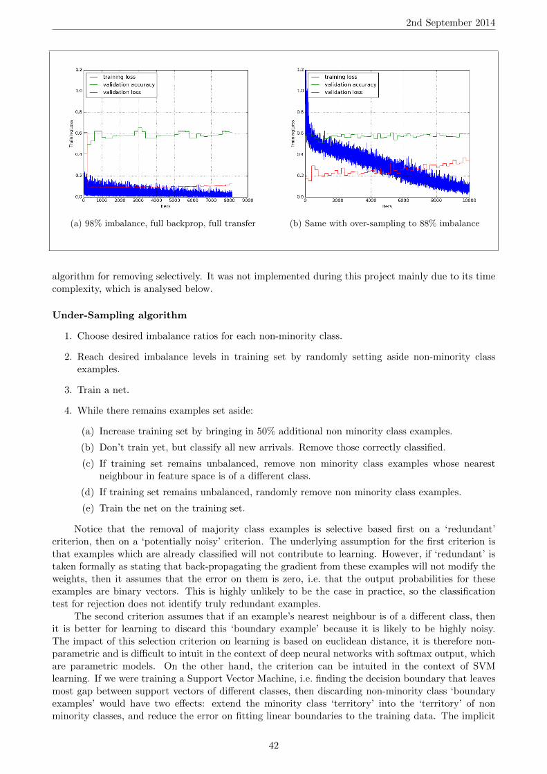
2nd September 2014

(a) 98% imbalance, full backprop, full transfer (b) Same with over-sampling to 88% imbalance

algorithm for removing selectively. It was not implemented during this project mainly due to its timecomplexity, which is analysed below.

Under-Sampling algorithm

1. Choose desired imbalance ratios for each non-minority class.

2. Reach desired imbalance levels in training set by randomly setting aside non-minority classexamples.

3. Train a net.

4. While there remains examples set aside:

(a) Increase training set by bringing in 50% additional non minority class examples.

(b) Don’t train yet, but classify all new arrivals. Remove those correctly classified.

(c) If training set remains unbalanced, remove non minority class examples whose nearestneighbour in feature space is of a different class.

(d) If training set remains unbalanced, randomly remove non minority class examples.

(e) Train the net on the training set.

Notice that the removal of majority class examples is selective based first on a ‘redundant’criterion, then on a ‘potentially noisy’ criterion. The underlying assumption for the first criterion isthat examples which are already classified will not contribute to learning. However, if ‘redundant’ istaken formally as stating that back-propagating the gradient from these examples will not modify theweights, then it assumes that the error on them is zero, i.e. that the output probabilities for theseexamples are binary vectors. This is highly unlikely to be the case in practice, so the classificationtest for rejection does not identify truly redundant examples.

The second criterion assumes that if an example’s nearest neighbour is of a different class, thenit is better for learning to discard this ‘boundary example’ because it is likely to be highly noisy.The impact of this selection criterion on learning is based on euclidean distance, it is therefore non-parametric and is difficult to intuit in the context of deep neural networks with softmax output, whichare parametric models. On the other hand, the criterion can be intuited in the context of SVMlearning. If we were training a Support Vector Machine, i.e. finding the decision boundary that leavesmost gap between support vectors of different classes, then discarding non-minority class ‘boundaryexamples’ would have two effects: extend the minority class ‘territory’ into the ‘territory’ of nonminority classes, and reduce the error on fitting linear boundaries to the training data. The implicit

42

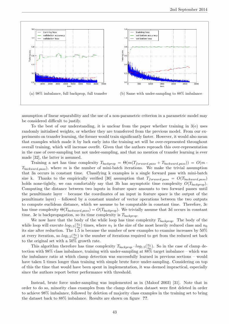
2nd September 2014

(a) 98% imbalance, full backprop, full transfer (b) Same with under-sampling to 88% imbalance

assumption of linear separability and the use of a non-parametric criterion in a parametric model maybe considered difficult to justify.

To the best of our understanding, it is unclear from the paper whether training in 3(e) usesrandomly initialised weights, or whether they are transferred from the previous model. From our ex-periments on transfer learning, the former would train significantly faster. However, it would also meanthat examples which made it by luck early into the training set will be over-represented throughoutoverall training, which will increase overfit. Given that the authors reproach this over-representationin the case of over-sampling but not under-sampling, and that no mention of transfer learning is evermade [32], the latter is assumed.

Training a net has time complexity Tbackprop = Θ(m(Tforward pass + Tbackward pass)) = O(m ·Tbackward pass), where m is the number of mini-batch iterations. We make the trivial assumptionthat 3a occurs in constant time. Classifying k examples is a single forward pass with mini-batchsize k. Thanks to the empirically verified [30] assumption that Tforward pass = O(Tbackward pass)holds none-tightly, we can comfortably say that 3b has asymptotic time complexity O(Tbackprop).Computing the distance between two inputs in feature space amounts to two forward passes untilthe penultimate layer – because the coordinates of an input in feature space is the output of thepenultimate layer) – followed by a constant number of vector operations between the two outputsto compute euclidean distance, which we assume to be computable in constant time. Therefore, 3chas time complexity Θ(Tbackward pass) = O(Tbackprop). We trivially assume that 3d occurs in constanttime. 3e is backpropagation, so its time complexity is Tbackprop.

We now have that the body of the while loop has time complexity Tbackprop. The body of thewhile loop will execute log1.5(n1

n0) times, where n1 is the size of the most heavily reduced class and n0

its size after reduction. The 1.5 is because the number of new examples to examine increases by 50%at every iteration, so log1.5(n1

n0) is the number of iterations required to get from the reduced set back

to the original set with a 50% growth rate.This algorithm therefore has time complexity Tbackprop · log1.5(n1

n0). So in the case of clamp de-

tection with 98% class imbalance, training with under-sampling at 88% target imbalance – which wasthe imbalance ratio at which clamp detection was successfully learned in previous sections – wouldhave taken 5 times longer than training with simple brute force under-sampling. Considering on topof this the time that would have been spent in implementation, it was deemed impractical, especiallysince the authors report better performance with threshold.

Instead, brute force under-sampling was implemented as in (Maloof 2003) [31]. Note that inorder to do so, minority class examples from the clamp detection dataset were first deleted in orderto achieve 98% imbalance, followed by deletion of majority class examples in the training set to bringthe dataset back to 88% imbalance. Results are shown on figure ??.

43

2nd September 2014

The results show that under-sampling is very effective: the model does not get stuck in anyseeming critical point, obtains an additional 15 percentage points in classification accuracy,to obtain80.8% validation accuracy. This is substantial and shows how strikingly detrimental class imbalanceis: we have eliminated 58.7% of the data to get rid of it, and yet this sacrifice is highly worthwhile.This sets a high benchmark for other techniques for tackling class imbalance. Since we are throwingdata, it also implies that if there exists a technique for solving class imbalance without losing data,performance could be even higher. The assumption that underlies this is that providing the modelwith additional information i.e. data is in theory purely beneficial, therefore there must exist a wayfor doing so.

6.4.6 Threshold-Moving

(Maloof 2003) and (Zhou and Liu 2005) both find threshold-moving to be the best technique fortackling class imbalance. It allows one to set different costs to mis-classifications on different classes; inthe 2-class case, this means that we can assign different costs to false positives than to false negatives.As with detecting the presence of a pathogen in a patient in the medical industry [34], one could arguethat a false negative is more expensive to ControlPoint: it is worse to classify a bad joint as goodthan to classify a good joint as bad, since in the latter case, no potential damage is done to the instal-lation. When the idea of assigning different costs was suggested to ControlPoint, the reply was positive.

Motivations Threshold-moving is a technique that operates on the model only at test time. It isimplemented by taking the predictions of the model at test time, dividing them by the prior probabil-ities of the classes i.e. their proportions in the training set, and renormalising. This may remind oneof Bayes’ theorem; indeed, threshold-moving has an elegant probabilistic interpretation. Consider amodel trained on a 2-class task with assignment of equal cost to both mis-classifications, and its outputon an example c from the test set. We would want the model to predict the label arg max

l∈l1,l2p(c|l).

However, the model will output the probabilities (p(l1|c), p(l2|c)) = (p(c|l1)p(l1), p(c|l2)p(l2). Themodel will output exactly what we want when classes are distributed uniformly in the training set,since the p(li) will all be the same. This fails if the priors are different, and can be corrected simply byexploiting Bayes’ theorem: dividing the output by the prior and renormalising. The reason for whythis is called threshold-moving can be explained as follows: assume the prior probability for class C1 isp(C1) = 0.1. The threshold for classifying in input as C1 given its predicted probability for belongingto C1 moves from 0.5 to 0.1.

Note that the mismatch between desired and outputted probabilities, exposed by this Bayesianconceptual framework, occurs as soon as classes are not uniformly distributed, which corresponds tothe literature’s definition of class imbalance rather than the definition of ‘dangerous’ class imbalanceproposed by this report. This has one of two implications: either – as the difference in definitionssuggest – probability mismatch and introduction of bad critical points in the error surface are twodifferent problems, or they are the same one, and the problems observed with class imbalance un-til now have been wrongly interpreted, wrongly explained. This can be verified by seeing whetherthreshold-moving solves this hypothetical bad critical point problem, i.e. if it stops the model fromoutputting the same classification for all inputs at test time.

Implementation Threshold-moving can be relatively easily implemented by writing a Python scriptthat runs a trained model on a test set, obtains the predicted probabilities, and classifies according tothe modified threshold, given by the prior probabilities of the classes. Also, if we choose to make thethreshold flexible rather than determined by the prior probabilities, then we have a way to increasethe relative cost of a false negative at will. This can be used to set a threshold that guarantees, say,95% accuracy on true positives, with a consequentially lower accuracy on true negatives dependingon the overall performance of the model. Note that practically, this would enable the automation of

44

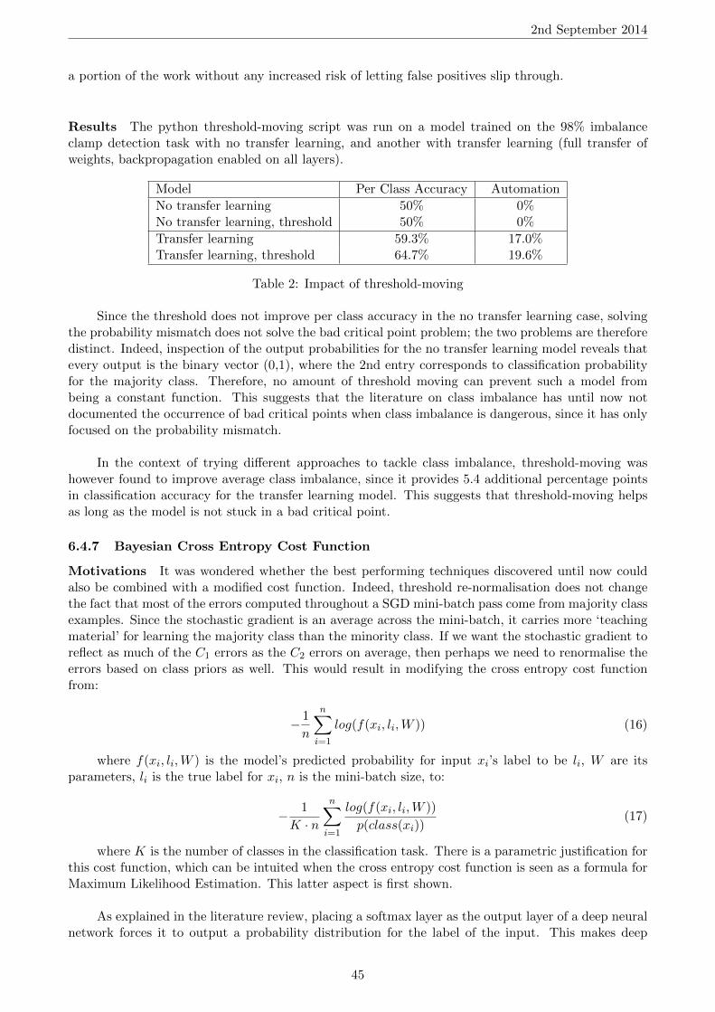
2nd September 2014

a portion of the work without any increased risk of letting false positives slip through.

Results The python threshold-moving script was run on a model trained on the 98% imbalanceclamp detection task with no transfer learning, and another with transfer learning (full transfer ofweights, backpropagation enabled on all layers).

Model Per Class Accuracy Automation

No transfer learning 50% 0%No transfer learning, threshold 50% 0%

Transfer learning 59.3% 17.0%Transfer learning, threshold 64.7% 19.6%

Table 2: Impact of threshold-moving

Since the threshold does not improve per class accuracy in the no transfer learning case, solvingthe probability mismatch does not solve the bad critical point problem; the two problems are thereforedistinct. Indeed, inspection of the output probabilities for the no transfer learning model reveals thatevery output is the binary vector (0,1), where the 2nd entry corresponds to classification probabilityfor the majority class. Therefore, no amount of threshold moving can prevent such a model frombeing a constant function. This suggests that the literature on class imbalance has until now notdocumented the occurrence of bad critical points when class imbalance is dangerous, since it has onlyfocused on the probability mismatch.

In the context of trying different approaches to tackle class imbalance, threshold-moving washowever found to improve average class imbalance, since it provides 5.4 additional percentage pointsin classification accuracy for the transfer learning model. This suggests that threshold-moving helpsas long as the model is not stuck in a bad critical point.

6.4.7 Bayesian Cross Entropy Cost Function

Motivations It was wondered whether the best performing techniques discovered until now couldalso be combined with a modified cost function. Indeed, threshold re-normalisation does not changethe fact that most of the errors computed throughout a SGD mini-batch pass come from majority classexamples. Since the stochastic gradient is an average across the mini-batch, it carries more ‘teachingmaterial’ for learning the majority class than the minority class. If we want the stochastic gradient toreflect as much of the C1 errors as the C2 errors on average, then perhaps we need to renormalise theerrors based on class priors as well. This would result in modifying the cross entropy cost functionfrom:

− 1

n

n∑i=1

log(f(xi, li,W )) (16)

where f(xi, li,W ) is the model’s predicted probability for input xi’s label to be li, W are itsparameters, li is the true label for xi, n is the mini-batch size, to:

− 1

K · n

n∑i=1

log(f(xi, li,W ))

p(class(xi))(17)

where K is the number of classes in the classification task. There is a parametric justification forthis cost function, which can be intuited when the cross entropy cost function is seen as a formula forMaximum Likelihood Estimation. This latter aspect is first shown.

As explained in the literature review, placing a softmax layer as the output layer of a deep neuralnetwork forces it to output a probability distribution for the label of the input. This makes deep

45

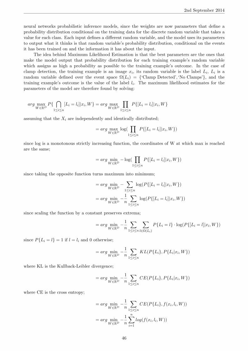
2nd September 2014

neural networks probabilistic inference models, since the weights are now parameters that define aprobability distribution conditional on the training data for the discrete random variable that takes avalue for each class. Each input defines a different random variable, and the model uses its parametersto output what it thinks is that random variable’s probability distribution, conditional on the eventsit has been trained on and the information it has about the input.

The idea behind Maximum Likelihood Estimation is that the best parameters are the ones thatmake the model output that probability distribution for each training example’s random variablewhich assigns as high a probability as possible to the training example’s outcome. In the case ofclamp detection, the training example is an image xi, its random variable is the label Li, Li is arandom variable defined over the event space Ω(Li) = ‘Clamp Detected’, ‘No Clamps’, and thetraining example’s outcome is the value of the label li. The maximum likelihood estimates for theparameters of the model are therefore found by solving:

arg maxW∈RD

P⋂

1≤i≤n[Li = li]|xi,W = arg max

W∈RD

∏1≤i≤n

P[Li = li]|xi,W

assuming that the Xi are independently and identically distributed;

= arg maxW∈RD

log(∏

1≤i≤nP[Li = li]|xi,W)

since log is a monotonous strictly increasing function, the coordinates of W at which max is reachedare the same;

= arg minW∈RD

− log(∏

1≤i≤nP[Li = li]|xi,W)

since taking the opposite function turns maximum into minimum;

= arg minW∈RD

−∑

1≤i≤nlog(P[Li = li]|xi,W)

= arg minW∈RD

− 1

n

∑1≤i≤n

log(P[Li = li]|xi,W)

since scaling the function by a constant preserves extrema;

= arg minW∈RD

− 1

n

∑1≤i≤n

∑l∈Ω(Li)

PLi = l · log(P[Li = l]|xi,W)

since PLi = l = 1 if l = li and 0 otherwise;

= arg minW∈RD

− 1

n

∑1≤i≤n

KL(PLi, PLi|xi,W)

where KL is the Kullback-Leibler divergence;

= arg minW∈RD

− 1

n

∑1≤i≤n

CE(PLi, PLi|xi,W)

where CE is the cross entropy;

= arg minW∈RD

− 1

n

∑1≤i≤n

CE(PLi, f(xi, li,W ))

= arg minW∈RD

− 1

n

n∑i=1

log(f(xi, li,W ))

46

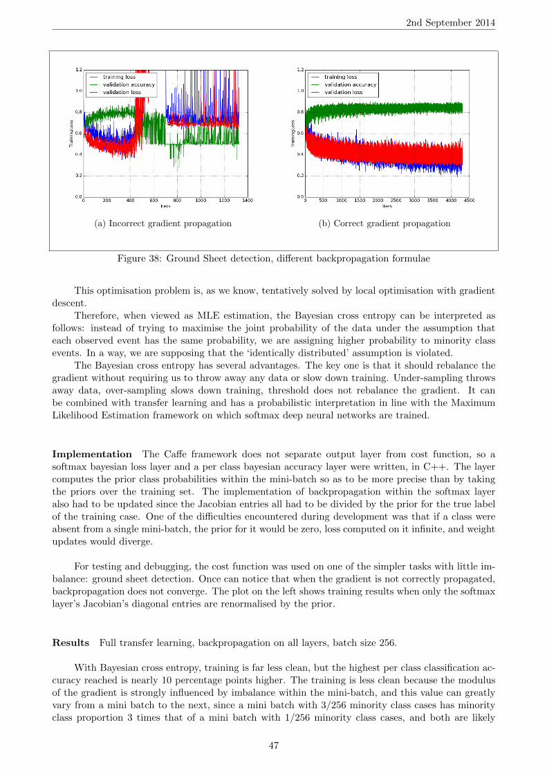
2nd September 2014

(a) Incorrect gradient propagation (b) Correct gradient propagation

Figure 38: Ground Sheet detection, different backpropagation formulae

This optimisation problem is, as we know, tentatively solved by local optimisation with gradientdescent.

Therefore, when viewed as MLE estimation, the Bayesian cross entropy can be interpreted asfollows: instead of trying to maximise the joint probability of the data under the assumption thateach observed event has the same probability, we are assigning higher probability to minority classevents. In a way, we are supposing that the ‘identically distributed’ assumption is violated.

The Bayesian cross entropy has several advantages. The key one is that it should rebalance thegradient without requiring us to throw away any data or slow down training. Under-sampling throwsaway data, over-sampling slows down training, threshold does not rebalance the gradient. It canbe combined with transfer learning and has a probabilistic interpretation in line with the MaximumLikelihood Estimation framework on which softmax deep neural networks are trained.

Implementation The Caffe framework does not separate output layer from cost function, so asoftmax bayesian loss layer and a per class bayesian accuracy layer were written, in C++. The layercomputes the prior class probabilities within the mini-batch so as to be more precise than by takingthe priors over the training set. The implementation of backpropagation within the softmax layeralso had to be updated since the Jacobian entries all had to be divided by the prior for the true labelof the training case. One of the difficulties encountered during development was that if a class wereabsent from a single mini-batch, the prior for it would be zero, loss computed on it infinite, and weightupdates would diverge.

For testing and debugging, the cost function was used on one of the simpler tasks with little im-balance: ground sheet detection. Once can notice that when the gradient is not correctly propagated,backpropagation does not converge. The plot on the left shows training results when only the softmaxlayer’s Jacobian’s diagonal entries are renormalised by the prior.

Results Full transfer learning, backpropagation on all layers, batch size 256.

With Bayesian cross entropy, training is far less clean, but the highest per class classification ac-curacy reached is nearly 10 percentage points higher. The training is less clean because the modulusof the gradient is strongly influenced by imbalance within the mini-batch, and this value can greatlyvary from a mini batch to the next, since a mini batch with 3/256 minority class cases has minorityclass proportion 3 times that of a mini batch with 1/256 minority class cases, and both are likely

47

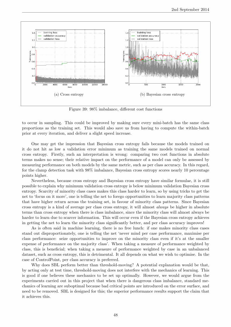
2nd September 2014

(a) Cross entropy (b) Bayesian cross entropy

Figure 39: 98% imbalance, different cost functions

to occur in sampling. This could be improved by making sure every mini-batch has the same classproportions as the training set. This would also save us from having to compute the within-batchprior at every iteration, and deliver a slight speed increase.

One may get the impression that Bayesian cross entropy fails because the models trained onit do not hit as low a validation error minimum as training the same models trained on normalcross entropy. Firstly, such an interpretation is wrong: comparing two cost functions in absoluteterms makes no sense; their relative impact on the performance of a model can only be assessed bymeasuring performance on both models by the same metric, such as per class accuracy. In this regard,for the clamp detection task with 98% imbalance, Bayesian cross entropy scores nearly 10 percentagepoints higher.

Nevertheless, because cross entropy and Bayesian cross entropy have similar formulae, it is stillpossible to explain why minimum validation cross entropy is below minimum validation Bayesian crossentropy. Scarcity of minority class cases makes this class harder to learn, so by using tricks to get thenet to ‘focus on it more’, one is telling the net to forego opportunities to learn majority class patternsthat have higher return across the training set, in favour of minority class patterns. Since Bayesiancross entropy is a kind of average per class cross entropy, it will almost always be higher in absoluteterms than cross entropy when there is class imbalance, since the minority class will almost always beharder to learn due to scarcer information. This will occur even if the Bayesian cross entropy achievesin getting the net to learn the minority class significantly better, and per class accuracy improves!

As is often said in machine learning, there is no free lunch: if one makes minority class casesstand out disproportionately, one is telling the net ‘never mind per case performance, maximise perclass performance: seize opportunities to improve on the minority class even if it’s at the smallerexpense of performance on the majority class’. When taking a measure of performance weighted byclass, this is beneficial; when taking a measure of performance weighted by case in an unbalanceddataset, such as cross entropy, this is detrimental. It all depends on what we wish to optimise. In thecase of ControlPoint, per class accuracy is preferred.

Why does SBL perform better than threshold-moving? A potential explanation would be that,by acting only at test time, threshold-moving does not interfere with the mechanics of learning. Thisis good if one believes these mechanics to be set up optimally. However, we would argue from theexperiments carried out in this project that when there is dangerous class imbalance, standard me-chanics of learning are suboptimal because bad critical points are introduced on the error surface, andneed to be removed. SBL is designed for this; the superior performance results support the claim thatit achieves this.

48

2nd September 2014

Further Research It would be interesting to mathematically derive how imbalance affects themodulus of the gradient, and how the standard deviation of the modulus with with Bayesian crossentropy is much greater than with cross entropy. As mentioned, the variance of the gradient couldalso be reduced by making sure every mini-batch has the same class proportions as the training set.This would also save us from having to compute the within-batch prior at every iteration, and delivera slight speed increase.

It would also be interesting to confirm that Bayesian cross entropy achieves something differentto threshold-moving. This could be achieved with the threshold-moving Python script, which containscode that, given a model and target ratio of false positives to total positives, returns the proportionof predicted negatives, when the threshold level that is required to attain this target ratio is used.The extent to which this proportion is greater for the model trained with Bayesian cross entropy thanfor the same model trained with cross entropy would be a measure of the additional semantic contentlearned.

Overall, these results are encouraging and further experiments with benchmark multi-class datasetssuch as MNIST, CIFAR and ImageNet would allow to situate the performance gains from using SBLin a wider academic context.

6.4.8 Error-accuracy mismatch revisited

A surprising observation made on all previous training results was that per class accuracy tendsto continue improving long after the validation error begins to deteriorate. A proposed explanationwas that, during this period, the model increases its precision on the minority class at the slightexpense of precision on the majority class. It was based on the mismatch between averaging the per-formance metric across the dataset and averaging across classes. In the training results for Bayesiancross entropy, the validation error is also averaged per class, and indeed, error and accuracy appearstrongly negatively correlated. This is substantial evidence in favour of this explanation.

However, what remains a curiosity are the implications that this explanation has for the dynamicsof learning: it would imply that when using cross entropy error, learning ‘focuses’ on the majorityclass first, and afterwards focuses on learning the minority class. This makes ‘strategic’ sense, sincethere are more gains from improving on the majority class when using an error that is averaged acrossthe min-batch.

SGD mechanics One may wonder how this could translate from the mechanics of Stochastic Gra-dient Descent. In the two class case, for each softmax neuron, the gradient propagating through itin a class A instance is always of opposite sign to that from a class B instance. Therefore, whenbackpropagating a gradient that has been averaged over a mini-batch with class imbalance, assumingthat the average per-case error on the majority class is sufficiently not smaller than on the minorityclass, then this averaged gradient will be of the same sign as a majority class gradient. Therefore,the weight corrections for the softmax layer will be in the direction that favours learning the majorityclass over the minority class. Assuming that class imbalance is present in all mini-batches, this willoccur until the per-case error on the majority class is sufficiently reduced as to change the sign of theaveraged ‘stochastic’ gradient, and invert the directions of learning in the softmax layer in favour ofthe minority class14.

All of the above holds only for the softmax output layer and not for lower layers, since as shownin the section on the ReLU, the sign of a gradient propagating from one neuron to another will changeif the edge it is propagating through has negative weight. Therefore, the above cannot explain how theentire model learns. Nevertheless, it provides some analytical grounding for what is being observed.Observing and analysing these mechanisms further and with greater rigour would perhaps make forinteresting further research.

14All these affirmations can be shown analytically, but due to time constraints were not written up in this report.

49

2nd September 2014

7 Conclusions and Future Work

The third stage of the empirical research focused on formalising class imbalance, understandinghow it impacts learning, and seeking ways to deal with it. Despite its dire effects, the topic is signif-icantly undocumented in the field of deep learning, so the research was an opportunity to make newinsights and discoveries. It seems that when the distribution of classes in the training set are such thata classifier which constantly outputs the class priors can obtain high performance, the error surfaceassociated with standard cost functions is punctured with bad sampling-induced critical points, whichslow down and often even prevent learning with stochastic gradient descent. After exploring simpletechniques as well as some of those advocated by the literature, a novel cost function was proposed. Itsability to tackle class imbalance was found to be substantial, delivering up to 28 additional percentagepoints in average per class validation accuracy in imbalanced tasks. The performance gains from thisBayesian cross entropy are also likely to be increased by ensuring the same distribution of classes inevery mini-batch of the training set, since this would reduce noisiness a.k.a variance in the modulusof the gradient. Further empirical research would also need to be conducted by trying out this costfunction on benchmark datasets with multiple classes and varying levels of class imbalance.

50

2nd September 2014

References

[1] Krizhevsky, Alex; Sutskever, Ilya; Hinton, Geoffrey E.; ImageNet Classification with Deep Convo-lutional Neural Networks2012

[2] Glorot, Xavier; Bordes, Antoine; Bengio, Yoshua; Deep Sparse Rectifier Neural Networks2013

[3] Lowe, David Object Recognition From Local Scale-Invariant FeaturesThe Proceedings of the Seventh IEEE International Conference on Computer Vision 1999

[4] Ian J. Goodfellow, Yaroslav Bulatov, Julian Ibarz, Sacha Arnoud, Vinay Shet Multi-digit NumberRecognition from Street View Imagery using Deep Convolutional Neural NetworksILSVRC 2013

[5] Tang, Yichuan; Deep Learning using linear Support Vector MachinesarXiv 2014

[6] Nair, Vinod; Hinton, Geoffrey; Rectified Linear Units Improve Restricted Boltzmann MachinesICML 2010

[7] G. E. Hinton, N. Srivastava, A. Krizhevsky, I. Sutskever and R. R. Salakhutdinov; ImprovingNeural Networks By Preventing Co-Adaptation of Feature DetectorsarXiv 2012

[8] Dan C. Ciresan, Ueli Meier, Jonathan Masci, Luca M. Gambardella, Juergen Schmidhuber; High-Performance Neural Networks for Visual Object ClassificationarXiv 2011

[9] Donahue, Jeff; Jia, Yangqing; Vinyals, Oriol; Hoffman, Judy; Zhang, Ning; Tzeng, Eric; Darrell,Trevor; DeCAF: A Deep Convolutional Activation Feature for Generic Visual RecognitionarXiv preprint arXiv:1310.1531, 2013

[10] Fergus, Robert; Tutorials Session A - Deep Learning for Computer VisionNIPS 2013

[11] Ali Sharif Razavian, Hossein Azizpour, Josephine Sullivan, Stefan Carlsson; CNN Features off-the-shelf: an Astounding Baseline for RecognitionarXiv 2014

[12] Olah, Christopher; Understanding ConvolutionsURL: http://colah.github.io/posts/2014-07-Understanding-Convolutions/, last accessed1st September 2014.

[13] Zhou, Zhi-Hua; Zhang, Min-Ling; Multi-Instance Multi-Label Learning with Application to SceneClassificationAdvances in Neural Information Processing Systems 19, Proceedings of the Twentieth AnnualConference on Neural Information Processing Systems, Vancouver, British Columbia, Canada,December 4-7, 2006

[14] Fusion Group - ControlPoint LLP, Company DescriptionURL: http://www.fusionprovida.com/companies/control-pointlast accessed 5th June 2014.

[15] LeCun, Yann; The Unreasonable Effectiveness of Deep LearningJournee du Labez Bexout 12 June 2014 URL: https://www.youtube.com/watch?v=zPVHH7ZJi9Q&list=PLYTk9IwHBb2ANKHc2feIso7tL1slpuVPY&index=1

last accessed 4th September 2014/

51

2nd September 2014

[16] Barron, Andrew R., Universal Approximation Bounds for Superpositions of a Sigmoidal FunctionIEEE Transactions on Information Theory, Vol. 39, No. 3 May 1993

[17] Bengio, Yoshua; Learning Deep Architectures for AIFoundations and Trends in Machine Learning Vol. 2, No. 1 (2009) 1-127 2009

[18] Bishop, Christopher; Pattern Recognition and Machine LearningSpringer 2010

[19] Zeiler, Matthew; Fergus, Robert; Visualizing and Understanding Convolutional NetworksarXiv 2013

[20] Russell, Stuart J; Norvig, Peter; Artificial Intelligence: A Modern Approach2003

[21] Hornik, Kur; Stinchcombe, Maxwell; White, Halber; Multilayer Feed-Forward Networks are Uni-versal Approximators1989

[22] Saenko, K., Kulis, B., Fritz, M., and Darrell, T.; Adapting visual category models to new domainsECCV, 2010

[23] Bengio, Yoshua; Google+ Deep Learning community postURL: https://plus.google.com/+YoshuaBengio/posts/GJY53aahqS8, last accessed 1stSeptember 2014.

[24] Bay, H., Tuytelaars, T., and Gool, L. Van; SURF: Speeded up robust featuresECCV, 2006

[25] Sermanet, Pierre; Eigen, David; Zhang, Xiang; Mathieu, Michael; Fergus, Rob; LeCun, Yann;OverFeat: Integrated Recognition, Localization and Detection using Convolutional NetworksarXiv:1312.6229

[26] Krizhevsky, Alex; Cuda-ConvNet: High-performance C++/CUDA implementation of convolu-tional neural networksURL: https://code.google.com/p/cuda-convnet/, last accessed 6th June 2014.

[27] Deng, Li; Yu, Dong; Deep Learning Methods and ApplicationsFoundations and Trends in Signal Processing 7:3-4 2014

[28] Jia, Yangqing; Caffe: a deep learning framework URL: http://caffe.berkeleyvision.org/getting_pretrained_models.html

last accessed 6th June 2014.

[29] Fergus, Robert; NIPS 2013 Tutorial - Deep Learning for Computer Vision, URL: http:

//research.microsoft.com/apps/video/default.aspx?id=206976&l=i

last accessed 6th August 2014.

[30] URL: https://github.com/soumith/convnet-benchmarkslast accessed 2nd September 2014.

[31] Maloof, Marcus A; Learning when data sets are imbalanced and when costs are unequal andunknownWorkshop on Learning from Imbalanced Data Sets II, ICML 2003

[32] Zhi-Hua, Zhou; Xu-Ying, Liu; Training Cost-Sensitive Neural Networks with Methods Addressingthe Class Imbalance ProblemIEEE Transactions on Knowledge and Data Engineering, 2005

52

2nd September 2014

[33] Joan Pastor-Pellicer, Francisco Zamora-Martnez, Salvador Espaa-Boquera, Mara Jos Castro-Bleda; F-Measure as the Error Function to Train Neural NetworksAdvances in Computational Intelligence Volume 7902, 2013, pp 376-384

[34] He, Haibo; Learning from imbalanced dataIEEE Transactions on Knowledge and Data Engineering Volume 21, no 9, 2009

[35] Hinton, Geoffrey; Neural Networks for Machine LearningCoursera, URL: http://coursera.org/course/neuralnets

[36] Theano, URL: http://deeplearning.net/software/theano/

[37] Torch7, URL: http://torch.ch/

53