developing random compaction strategy for apache
TRANSCRIPT

Master of Science in Telecommunication SystemsFebruary 2021
Developing Random CompactionStrategy for Apache Cassandra
database and Evaluating performanceof the Strategy
Roop Sai Surampudi
Faculty of Engineering, Blekinge Institute of Technology, 371 79 Karlskrona, Sweden

This thesis is submitted to the Faculty of Engineering at Blekinge Institute of Technology inpartial fulfilment of the requirements for the degree of Master of Science in TelecommunicationSystems. The thesis is equivalent to 20 weeks of full time studies.
The authors declare that they are the sole authors of this thesis and that they have not usedany sources other than those listed in the bibliography and identified as references. They furtherdeclare that they have not submitted this thesis at any other institution to obtain a degree.
Contact Information:Author(s):Roop Sai SurampudiE-mail: [email protected]
External advisor:Per ÖtterstromEricssonKarlskrona, Sweden
University advisor:Siamak KhatibiDepartment of Aesthetics and Technology
Faculty of Engineering Internet : www.bth.seBlekinge Institute of Technology Phone : +46 455 38 50 00SE–371 79 Karlskrona, Sweden Fax : +46 455 38 50 57

Introduction: Nowadays, the data generated by the global communication sys-tems is enormously increasing. There is a need by Telecommunication Industries tomonitor and manage this data generation efficiently. Apache Cassandra is a NoSQLdatabase which manages any formatted data and a massive amount of data flowefficiently.
Aim: This project is focused on developing a new random compaction strategy andevaluating this random compaction strategy’s performance. In this study, limita-tions of generic compaction strategies Size Tiered Compaction Strategy and LeveledCompaction Strategy will be investigated. A new random compaction strategy willbe developed to address the limitations of the generic Compaction Strategies. Im-portant performance metrics required for evaluation of the strategy will be studied.
Method: In this study, a grey literature review is done to understand the workingof Apache Cassandra, different compaction strategies’ APIs. A random compactionstrategy is developed in two phases of development. A testing environment is cre-ated consisting of a 4-node cluster and a simulator. Evaluated the performance bystress-testing the cluster using different workloads.
Results: A stable RCS artefact is developed. This artefact also includes supportof generating random threshold from any user-defined distribution. Currently, onlyUniform, Geometric, and Poisson distributions are supported. The RCS-Uniform’sperformance is found to be better than both STCS and LCS. The RCS-Poisson’s per-formance is found to be not better than both STCS and LCS. The RCS-Geometric’sperformance is found to be better than STCS.
Keywords: Apache Cassandra, Compaction, Random Probability Distributions,IBM Cloud, NoSQL databases

Acknowledgments
I would like to express my sincere gratitude to my supervisor, Siamak Khatibi, forhis continuous guidance and support to achieve this project’s aim.
I want to thank Annika Görling for providing me with this excellent thesis topic.
I express my sincere gratitude to Per Otterström for supervising me from the in-dustry side.
I would like to thank all my friends, parents and my beloved ones for their con-tinuous support.
ii

Contents
Acknowledgments ii
1 Introduction 11.1 Problem Statement and Motivation . . . . . . . . . . . . . . . . . . . 11.2 Aim . . . . . . . . . . . . . . . . . . . . . . . . . . . . . . . . . . . . 21.3 Objectives . . . . . . . . . . . . . . . . . . . . . . . . . . . . . . . . . 21.4 Research Questions . . . . . . . . . . . . . . . . . . . . . . . . . . . . 21.5 Document Outline . . . . . . . . . . . . . . . . . . . . . . . . . . . . 3
2 Background 52.1 Apache Cassandra . . . . . . . . . . . . . . . . . . . . . . . . . . . . 52.2 Architecture of Cassandra . . . . . . . . . . . . . . . . . . . . . . . . 6
2.2.1 Peer-to-Peer Architecture . . . . . . . . . . . . . . . . . . . . 62.3 Generic Compaction Strategies . . . . . . . . . . . . . . . . . . . . . 72.4 Key Components of Apache Cassandra Database . . . . . . . . . . . 92.5 Write Path . . . . . . . . . . . . . . . . . . . . . . . . . . . . . . . . 102.6 Read Path . . . . . . . . . . . . . . . . . . . . . . . . . . . . . . . . . 112.7 Different Tools Used in this project . . . . . . . . . . . . . . . . . . . 12
2.7.1 CQL & CQLSH . . . . . . . . . . . . . . . . . . . . . . . . . . 122.7.2 Default Cassandra-Stress Tool . . . . . . . . . . . . . . . . . . 132.7.3 Node Exporter . . . . . . . . . . . . . . . . . . . . . . . . . . 132.7.4 Cassandra Metrics Exporter . . . . . . . . . . . . . . . . . . . 132.7.5 Prometheus & Grafana . . . . . . . . . . . . . . . . . . . . . . 132.7.6 IBM Cloud . . . . . . . . . . . . . . . . . . . . . . . . . . . . 13
3 Related Work 14
4 Method 164.1 Literature Review . . . . . . . . . . . . . . . . . . . . . . . . . . . . . 16
4.1.1 Search Strategy . . . . . . . . . . . . . . . . . . . . . . . . . . 174.1.2 Digital Libraries . . . . . . . . . . . . . . . . . . . . . . . . . . 174.1.3 Inclusion-Exclusion Criteria . . . . . . . . . . . . . . . . . . . 17
4.2 Development of new Compaction Strategy . . . . . . . . . . . . . . . 184.2.1 Phase 1 of Development . . . . . . . . . . . . . . . . . . . . . 184.2.2 Phase 2 of Development . . . . . . . . . . . . . . . . . . . . . 18
4.3 Testing the Developed Strategy . . . . . . . . . . . . . . . . . . . . . 194.3.1 Test Environment Setup . . . . . . . . . . . . . . . . . . . . . 194.3.2 Operating the Cassandra Cluster . . . . . . . . . . . . . . . . 21
iii

4.4 Data Collection . . . . . . . . . . . . . . . . . . . . . . . . . . . . . . 234.5 Performance Metrics . . . . . . . . . . . . . . . . . . . . . . . . . . . 23
4.5.1 Cassandra Metrics . . . . . . . . . . . . . . . . . . . . . . . . 244.5.2 Operating System Metrics . . . . . . . . . . . . . . . . . . . . 24
4.6 Data Analysis . . . . . . . . . . . . . . . . . . . . . . . . . . . . . . . 244.6.1 Statistical Test . . . . . . . . . . . . . . . . . . . . . . . . . . 24
5 Results 265.1 RQ1-Development of Random Compaction Strategy . . . . . . . . . . 26
5.1.1 Phase 1 of development . . . . . . . . . . . . . . . . . . . . . 265.1.2 Phase 2 of development . . . . . . . . . . . . . . . . . . . . . 27
5.2 RQ2 - Evaluating the performance of Compaction Strategies underdifferent workloads . . . . . . . . . . . . . . . . . . . . . . . . . . . . 295.2.1 Cassandra Metrics - Live SSTables & SSTables Per Read . . . 295.2.2 Operating System Metrics - CPU Utilization & Disk Space
Utilization . . . . . . . . . . . . . . . . . . . . . . . . . . . . . 405.2.3 Cassandra Performance Metric - Operation Latency . . . . . . 48
6 Discussion 506.1 Answers to Research Questions . . . . . . . . . . . . . . . . . . . . . 50
6.1.1 RQ1: How a compaction strategy can be developed in such away the compaction strategy compacts a random number ofSSTables . . . . . . . . . . . . . . . . . . . . . . . . . . . . . . 50
6.1.2 RQ2: How the performance of developed random compactionstrategy can be evaluated . . . . . . . . . . . . . . . . . . . . 50
6.2 Threats to Validity . . . . . . . . . . . . . . . . . . . . . . . . . . . . 516.2.1 Internal Validity . . . . . . . . . . . . . . . . . . . . . . . . . 516.2.2 Conclusion Validity . . . . . . . . . . . . . . . . . . . . . . . . 51
6.3 Limitations . . . . . . . . . . . . . . . . . . . . . . . . . . . . . . . . 51
7 Conclusions and Future Work 537.1 Conclusions . . . . . . . . . . . . . . . . . . . . . . . . . . . . . . . . 537.2 Future Work . . . . . . . . . . . . . . . . . . . . . . . . . . . . . . . . 54
A Supplemental Information 58
iv

List of Figures
2.1 Architecture of Apache Cassandra . . . . . . . . . . . . . . . . . . . . 62.2 Compaction in Apache Cassandra . . . . . . . . . . . . . . . . . . . . 72.3 Compaction Process Using STCS . . . . . . . . . . . . . . . . . . . . 82.4 SSTables residing on the disk after several Inserts using STCS . . . . 82.5 Compaction process using LCS . . . . . . . . . . . . . . . . . . . . . 92.6 SSTables after several Write requests using LCS . . . . . . . . . . . . 92.7 Write Path of Apache Cassandra . . . . . . . . . . . . . . . . . . . . 112.8 Read Path of Apache Cassandra . . . . . . . . . . . . . . . . . . . . . 12
4.1 Research Methodology . . . . . . . . . . . . . . . . . . . . . . . . . . 164.2 Network Architecture . . . . . . . . . . . . . . . . . . . . . . . . . . . 204.3 Software Installed in virtual server instances . . . . . . . . . . . . . . 21
5.1 Random Compaction Strategy’s Working Algorithm . . . . . . . . . . 285.2 Live SSTables & SSTables Per Read under WRITE, READ and MIXED
Workloads (Size Tiered Compaction Strategy) . . . . . . . . . . . . . 305.3 Live SSTables & SSTables Per Read under WRITE, READ and MIXED
Workloads (Leveled Compaction Strategy) . . . . . . . . . . . . . . . 315.4 Live SSTables & SSTables Per Read under WRITE, READ and MIXED
Workloads (Random Compaction Strategy - Uniform Distribution) . . 325.5 Live SSTables & SSTables Per Read under WRITE, READ and MIXED
Workloads (Random Compaction Strategy - Poisson Distribution) . . 345.6 Live SSTables & SSTables Per Read under WRITE, READ and MIXED
Workloads (Random Compaction Strategy - Geometric Distribution) 355.7 Average number of Live SSTables . . . . . . . . . . . . . . . . . . . . 375.8 SSTables Per READ . . . . . . . . . . . . . . . . . . . . . . . . . . . 395.9 CPU Utilization and Disk Space Utilization under WRITE, READ
and MIXED Workloads (Size Tiered Compaction Strategy) . . . . . . 415.10 CPU usage and Disk Space Usage under WRITE, READ and MIXED
Workloads (Leveled Compaction Strategy) . . . . . . . . . . . . . . . 425.11 CPU usage and Disk Space Usage under WRITE, READ and MIXED
Workloads (Random Compaction Strategy - Uniform Distribution) . . 435.12 CPU usage and Disk Space Usage under WRITE, READ and MIXED
Workloads (Random Compaction Strategy - Poisson Distribution) . . 445.13 CPU usage and Disk Space Usage under WRITE, READ and MIXED
Workloads (Random Compaction Strategy - Geometric Distribution) 455.14 Comparison of Average CPU Utilisation under different heavy workloads 485.15 Operation Latency . . . . . . . . . . . . . . . . . . . . . . . . . . . . 49
v
List of Tables
4.1 Hardware Specifications of Virtual Server Instances . . . . . . . . . . 19
5.1 Live SSTables - WRITE HEAVY Workload . . . . . . . . . . . . . . . 365.2 Live SSTables - READ HEAVY Workload . . . . . . . . . . . . . . . 375.3 Live SSTables - MIXEd HEAVY Workload . . . . . . . . . . . . . . . 375.4 One Way ANOVA Test for Live SSTables . . . . . . . . . . . . . . . . 385.5 SSTables Per READ - READ HEAVY Workload . . . . . . . . . . . . 385.6 SSTables Per READ - MIXED HEAVY Workload . . . . . . . . . . . 395.7 One Way ANOVA Test for SSTables Per READ . . . . . . . . . . . . 405.8 Summary Statistics - CPU Usage under WRITE heavy workload on
application of different compaction strategies . . . . . . . . . . . . . . 465.9 Summary Statistics - CPU Usage under READ heavy workload on
application of different compaction strategies . . . . . . . . . . . . . . 475.10 Summary Statistics - CPU Usage under MIXED heavy workload on
application of different compaction strategies . . . . . . . . . . . . . . 475.11 One Way ANOVA Test for CPU Utilization . . . . . . . . . . . . . . 485.12 Summary Statistics - Operation Latency under WRITE heavy work-
load on application of different compaction strategies . . . . . . . . . 495.13 Summary Statistics - Operation Latency under READ heavy workload
on application of different compaction strategies . . . . . . . . . . . . 49
1

List of Abbreviations
STCS Size Tiered Compaction Strategy
LCS Leveled Compaction Strategy
RCS-Uniform Random Compaction Strategy, in which random threshold is gener-ated from discrete Uniform Distribution. This threshold decides thenumber of SSTables to be compacted.
RCS-Poisson Random Compaction Strategy, in which random threshold is gener-ated from Poisson Distribution.
RCS-Geometric
Random Compaction Strategy, in which random threshold is gener-ated from Geometric Distribution.
SSD Solid-state device
HDD Hard disk drive
IT Information Technology
SSTable SortedString Table
GB Gigabyte
MB Megabyte
2

Chapter 1Introduction
Nowadays the Internet usage by the users is increasing tremendously. Consequently,data generation is also growing tremendously. The data generated each day can beof any format which includes unstructured, semi-structured and structured. Thereis a need by Telecommunication Industries, IT industries to store, manage, monitor,retrieve data efficiently and effectively. To effectively store, manage, and monitor thedata, there is a need for database management systems by IT industries. DatabaseManagement Systems plays a crucial role in Telecommunication Industries [14].
In the recent past, different database management systems are emerging and evolvingfast to systematically and spontaneously tackle the growing varieties and vagaries ofdata structures, schema, sizes, speeds, and scopes [26]. The database managementsystems fall under two categories.
• Relational Database Management Systems (RDBMS)
• NoSQL Databases (non-relational DBMS)
NoSQL databases are being used by almost every large organization to manage BigData efficiently. Big data is the general term used to represent massive amounts ofdata that are not stored in the relational form in traditional enterprise-scale SQLdatabases [14, 26]. Apache Cassandra is one of the NoSQL databases developed atFacebook to power their inbox search feature [15]. Apache Cassandra is an open-source distributed database management system designed to handle vast amounts ofany formatted data, including unstructured, structured and semi-structured formats.Apache Cassandra stores the persistent data in the form of immutable files calledSSTables. As these SSTables are immutable, they can’t be altered directly. ApacheCassandra uses a method called Compaction to reclaim the disk space and to improvethe performance of the database [5].This thesis project is part of the thesis project Creation of Random CompactionStrategies for Apache Cassandra database at Ericsson. Another Random CompactionStrategy for Apache Cassandra database is described in the paper [13].
1.1 Problem Statement and MotivationIn earlier versions of Apache Cassandra, two generic compaction strategies weredeveloped. These strategies are Size Tiered Compaction Strategy and Leveled Com-paction Strategy. These strategies are developed to improve the performance of the
1

Chapter 1. Introduction 2
database. These compaction strategies have significant limitations which can degradethe performance of the database in the long run. To overcome these limitations, de-veloping a new compaction strategy is needed. This thesis addresses the limitationsof these strategies and alternate solutions to overcome these limitations. This thesisfocuses on the development of a new compaction strategy. Moreover, this compactionstrategy is named as Random Compaction Strategy.
1.2 AimThe main aim of this project is to address the limitations of generic compactionstrategies and to develop a new random compaction strategy to overcome thoselimitations.
1.3 ObjectivesThe main objectives/goals to achieve the aim of this project are discussed as follows:
• Investigate the working of Compaction and compaction strategies.
• Investigate the limitations of Size Tiered Compaction Strategy and LeveledCompaction Strategies.
• Investigate which parameters are involved in effecting the Compaction.
• Based on the knowledge of APIs of generic compaction strategies and differentparameters involved in Compaction develop a new random compaction strategythat will not break Apache Cassandra’s functionality.
• Investigate which metrics are useful for the evaluation of the performance ofthe new compaction strategy.
• Evaluate the developed compaction strategy’s performance by comparing thedeveloped compaction strategy’s performance metrics with generic compactionstrategies.
1.4 Research Questions1. How can a new compaction strategy be developed so a random number of
SSTables will be compacted whenever a compaction process is triggered?Method Used To answer this question, conducted a detailed literature review,to gain knowledge on Apache Cassandra database APIs and generic compactionstrategies APIs. Based on these APIs, a new compaction strategy API isdeveloped from scratch. Meetings with Ericsson’s CIL team and advisor atBTH are conducted to gain more knowledge regarding compaction strategiesand how the randomness properties can be applied in creating a compactionstrategy.

Chapter 1. Introduction 3
2. How the performance of developed random compaction strategy can be evalu-ated?Method Used To answer this question, conducted focus meetings with Eric-sson’s CIL team and supervisor. Based on the Ericsson CIL team’s supervisorand team members’ opinions, the most useful performance metrics are consid-ered. By simulating different workloads, collecting the performance metrics,and comparing strategies using the metrics collected, the Random CompactionStrategy’s performance is evaluated.
1.5 Document OutlineThis document is organized as described below:
Chapter 1 Introduction
In this chapter, an overview of Apache Cassandra is given. This chapter exposes theaim of the thesis project. The research questions framed for this project are alsoprovided in this chapter.
Chapter 2 Background
In this chapter, an overview of databases is provided. This chapter exposes the trendof NoSQL databases in the Telecommunication & IT industries. In this chapter, thedata model, the architecture of Apache Cassandra is provided. The compactionmechanism and different compaction strategies implemented for Apache Cassandratill date and the significant limitations are depicted in this chapter.
Chapter 3 Related Work
This chapter exposes the related work done in the creation of Apache CompactionStrategies. In this chapter, the related work of evaluating the performance metricsfor Compaction Strategies is also mentioned.
Chapter 4 Method
This chapter exposes the methodologies administered to achieve the aim of theproject.
Chapter 5 Results and Analysis
This chapter depicts the results and analysis obtained from this project. The resultsand analysis are described in Graphical and tabular representations. This chapterillustrates the results obtained under different workloads for different compactionstrategies.

Chapter 1. Introduction 4
Chapter 6 Conclusions and Future Work
This chapter depicts the conclusions for the thesis work done. This chapter exposesthe future work that can be implemented.

Chapter 2Background
With the advent of digitization, Internet usage has tremendously increased in recentyears, leading to vast volumes of data with high velocity. Not only in terms of volume,but the data being generated is also of different forms (varieties) [25]. In the recentpast, Telecommunication Industries and IT industries used relational databases tomanage the information. The relational databases use structured schema to store thedata, and the relational database cannot support the management of unstructureddata. NoSQL databases have been proposed as a solution to storing the unstructureddata [26]. A NoSQL or Not Only SQL, which is a non-relational database designedto provide a mechanism for storage, management and retrieval of unstructured data,and it is faster than traditional SQL, as principles used by the NoSQL databases aredifferent from those principles of relational SQL, and it also makes data operationssuch as READ, WRITE operations faster when compared to relational databases.And NoSQL has a simple design and follows CAP Theorem instead of ACID princi-ples [1] and almost there are more than 225 different NoSQL databases widely usedby enterprises like Google, Yahoo, Amazon Twitter, Facebook, Ericsson and muchmore large IT Enterprises[22].
The most popular NoSQL databases are Wide Column Store, Key-Value Store, Doc-ument Store, and Graph Databases. Apache Cassandra belongs to the family ofKey-Value Store. As the name suggests the data in this particular database is storedin the format of "Key – Value", where the key is a string assigned with a uniquevalue for its identification and a value is an object which can be a string or numericvalue or even a complex binary large object[7].
2.1 Apache CassandraCassandra is a horizontally scalable and highly available NoSQL database, which fol-lows peer-to-peer networking architecture and the CAP theorem. Cassandra can beused to manage and store large volumes of unstructured, semi-structured and as wellas correctly structured data across various data centres while providing scalability,fault tolerance and high performance with no single point of failure[12].
5

Chapter 2. Background 6
2.2 Architecture of CassandraCassandra’s architecture follows peer to peer architecture(P2P), where within a clus-ter, the data can be replicated over multiple nodes. Nodes use Gossip Communi-cation Protocol to exchange information regarding state and location among them-selves. Due to data replication, the risk of a single point of failure is dropped tozero while providing high availability and scalability. In this architecture, commit-logs are used to ensure the durability of the data and data gets immediately storedin in-memory data structures, called memtables; upon memtables reaching a size ofconfigurable threshold (by default 123MB), it will be flushed into persistent disk stor-age as SSTable immutable data files. Cassandra uses a method called compaction,to periodically erase obsolete data from the persistent disk storage and improve theperformance of the READ operation [1].
Figure 2.1: Architecture of Apache Cassandra
2.2.1 Peer-to-Peer Architecture
Peer-to-peer architecture (P2P architecture) is the most widely used computer net-working architecture in which every Node has similar capabilities and responsibili-ties. Peer-to-peer architectures’ functionalities are often contrasted with client/servermodel architecture, where some particular systems(nodes) are confined to servingothers [3].

Chapter 2. Background 7
2.3 Generic Compaction StrategiesCompaction
Compaction method merges SSTables into one SSTable removing tombstones andreplacing old time-stamped data with updated data. Compaction plays a majorrole in improving the overall performance of the database. Compaction is triggeredautomatically by Cassandra to free the disk space and consequently improves theperformance of READ queries [27]. The compaction process is depicted in figure 2.2.
Figure 2.2: Compaction in Apache Cassandra
Size Tiered Compaction Strategy
The Size Tiered Compaction Strategy is the most widely used strategy by Telecom-munication Industries. Size Tiered Compaction Strategy merges SSTables of approx-imately the similar size. Similar sized SSTables are placed in buckets. Based uponthe hotness of the bucket, the SSTables in a hot bucket gets compacted[28]. Thecompaction process using STCS is depicted in figure 2.3. After several writes, smallnumber of SSTables are generated using STCS, it is depicted in figure 2.4. Variablesized SSTables are created using STCS.

Chapter 2. Background 8
Figure 2.3: Compaction Process Using STCS
Figure 2.4: SSTables residing on the disk after several Inserts using STCS
Limitations of Size Tiered Compaction Strategy
Compaction requires a lot of temporary space as the new larger SSTable is writtenbefore the duplicates are purged. In the worst-case up to half the disk space needs tobe empty to allow this to happen [2, 28]. This problem is referred to as Space Am-plification. In the past, to overcome Space Amplification problem IT Administratorsat Telecommunication Industries used to increase the number of disks attached to anode. In the past, the disk used is HDD which is cheaper compared to SSD beingused nowadays. Nowadays, increasing the number of disks(horizontal scaling)[23] isnot a viable solution.
Leveled Compaction Strategy
Leveled Compaction creates small, fixed-size (by default 160 MB) SSTables dividedinto different levels. Each level represents a run of a number of SSTables.To over-come space amplification limitation, the Leveled Compaction Strategy uses levelsand "Runs" for Compaction. "Run" refers to a group of SSTables, in which eachSSTable has a default size of 160MB[2, 28]. The compaction process using LeveledCompaction Strategy is depicted in figure 2.5. The SSTables created after com-paction using LCS resides in different runs. Most of the data reside on the last level.This is the main reason why READ performance is higher in the case of LCS. Mostof the time, it is just enough to query SSTables residing in the last level which ulti-mately makes the READ performance better and it is also depicted in the figure 2.6.The SSTables residing on disk after several write requests using LCS is depicted infigure 2.6.

Chapter 2. Background 9
Figure 2.5: Compaction process using LCS
Figure 2.6: SSTables after several Write requests using LCS
Limitations of Leveled Compaction Strategy
It consists of various levels, and as the levels go up, the number of SSTables in eachlevel increases by ten times the previous level. So, this won’t consume much spaceduring the compaction process. But due to less size of SSTables and levels, morecompactions are performed on the same data. The writing of the same rows, againand again, is called write amplification. Data written in one level is compacted tomultiple levels. Hence, a greater number of writes are done by the end that resultsin higher write amplification. Since this is correlated with read performance, theefficiency, on the whole, is affected. To this write amplification, more CPU cycles areutilized.Unnecessary usage of more CPU cycles are not recommended, and ultimatelyit consumes more power[13].
2.4 Key Components of Apache Cassandra DatabaseThe key components of Cassandra are described as follows[8]:
1. Node: Node is the most fundamental component of Cassandra where the datagets stored.
2. Datacenter: A datacenter is a group of related nodes, and Datacenter caneither be a physical or a virtual datacenter, depending on the replication factorsthe data can be replicated to multiple data centres.
3. Cluster: A cluster is a group of one or more data centres, and a cluster canbe spanned across all the physical locations where a data centre can not bespanned across all the physical locations.
4. Commit Log: During a write query, the data are initially written to the com-mit log for durability. Later, when the data is flushed into SSTables (persistentdisk storage), the data saved at the commit log gets deleted.

Chapter 2. Background 10
5. SSTables: Cassandra periodically flushes stored memtables to immutable datafiles, which are called SSTables.
6. Keyspaces: At the top level, the data in Cassandra is stored in the form ofkey spaces, where the keyspaces act as containers for tables, where the data inthe tables get stored in the form key-value pairs.
7. Gossip Communication Protocol: The gossip communication protocol isused in Cassandra to share information regarding state and location with othernodes inside the Cluster. Information within the nodes can be retrieved whennodes are restarted, as state information is persisted locally within the clusternodes.
8. Partitioner: The partitioner is a hash function used by Cassandra to deter-mine which Node gets the first replica of data. It also administers the distri-bution of data replicas across other cluster nodes, Murmur3Partitioner is thedefault Partitioner strategy and the most used strategy in all the use cases.
9. Replication factor: Replication factor is the total number of replicas of rowdata across the Cluster, and the replication factor is set per-table. For example,if RF=1, it means only one copy of data and does not provide fault tolerance.If RF=3, three similar copies of data are getting replicated across three nodesproviding higher availability and fault tolerance. For a single data centre, it ishighly recommended to use a replication factor of 3.
10. Replica Placement Strategy Apache Cassandra uses replica placement strat-egy to determine the selection of nodes on which should replicate the data.
11. Configuration Files Cassandra.yaml is the main configuration file that de-scribes the Cassandra Cluster’s entire configuration.
2.5 Write PathCassandra implements writing of data at various vital stages, starting from imme-diate logging of request to ensure durability and ends with the writing of persistentdata in immutable files called SSTables into the SSD or HDD. The figure 2.7 de-picts the write path of Apache Cassandra. The actual steps that involve the writingprocess are as follows[8]:
1. Logging requests and Memtable Storage: When any of the coordinator nodesreceives a WRITE request, the request is immediately logged in commit-log.Simultaneously, data is written in the form of an in-memory data structurecalled MemTable. Every incoming request is logged into the commit-log to en-sure durability. If a node fails due to any disaster, the data stored in Memtablegets lost. Each incoming request is logged in the commit-log, and when thenode comes back to live, the commit-log is replayed.
2. Flushing data from memtable: When the size of Memtable reaches a config-urable threshold limit, the memtable is flushed as SSTable into disk storage.

Chapter 2. Background 11
Figure 2.7: Write Path of Apache Cassandra
3. Storing data on disk in the form of SSTables: SSTables and Memtables aremaintained per table. The commit-log is shared between tables.SSTables areimmutable which once flushed from Memtable these SSTables cannot be up-dated in place. When a key-value pair is updated or created a new SSTableis created. Old time-stamped SSTables and unused SSTables are purged usingCompaction method of Apache Cassandra.
2.6 Read PathApache Cassandra uses complex data structures in both memory and disk to opti-mize read requests and reduce disk I/O operations[31]. The read path of ApacheCassandra is depicted in figure 2.8 Different data structures used by Cassandra toprocess a read request are as follows: Different data structures used by Cassandra toprocess a read request are as follows:
1. Memtable: Cassandra first searches the requested data in memtable. If itexists within memtable, the data within memtable combined with data withinSSTable is returned.
2. Row Cache: It is a data structure which stores a subset of data within SSTa-bles. As seeking the data from memory is faster than seeking from the disk,row cache boosts the READ performance.
3. Bloom Filter: If the partition key is not present in both Memtable and RowCache, Cassandra queries Bloom Filter to filter all SSTables where the keymight exist. Bloom Filter is a probabilistic data structure; it may sometimesreturn false positives.
4. Key Cache: It is an in-memory data structure which stores partition indices.If the requested partition key exists in Key Cache, the READ process directlyjumps to Compression Offset Map. It reduces disk seeks for a READ request.
5. Partition Summary: It is an in-memory data structure which stores a sampleof partition indices. If the key is not found in Key Cache, the process hits the

Chapter 2. Background 12
Figure 2.8: Read Path of Apache Cassandra
Partition Summary, and Cassandra searches for the range of possible partitionindices.
6. Partition Index: It is a data structure which resides on disk. Partition IndexStores the location of partition key on disk.
7. Compression Offset Map: Compression Offset Map Stores the pointers tothe location of requested data on disk. The data is returned from correctSSTables once the compression offset map identifies the location of data ondisk.
2.7 Different Tools Used in this project
2.7.1 CQL & CQLSH
Cassandra uses Cassandra Query language (CQL) as it is the primary interface tointeract with the database. Furthermore, CQLSH is used as the base to interactwith Cassandra. CQLSH being a primary interaction tool and also a powerful tool,where we can query any operation ranging from the creation of keyspace to dataoperations[8].

Chapter 2. Background 13
2.7.2 Default Cassandra-Stress Tool
Cassandra Stress Tool is a default stress testing utility provided by Apache Cassan-dra for load testing of a Cassandra cluster ranging from light workloads to heavyworkloads[8].
2.7.3 Node Exporter
Node exporter is an exporter provided by Prometheus to collect the operating systemand CPU metrics and also metrics related to hardware[24].
2.7.4 Cassandra Metrics Exporter
Cassandra metrics exporter is a java agent which exports the metrics of Cassan-dra to the Prometheus server, the performance of Cassandra exporter is better incomparison to JMX exporter[20].
2.7.5 Prometheus & Grafana
Prometheus is a monitoring and alerting software which is open source, and it alsoprovides multiple modes of graphing support. Moreover, time-series metrics canbe pulled easily using Prometheus; the setup of Prometheus is easy. The maincomponent of Prometheus is the Prometheus server, and its primary function is topull and store the time-series metrics in the specified data storage directory[24].
Grafana is a visualization tool and analytics software, which allows us to queryand visualize the metrics depending upon the data source provided[10].
2.7.6 IBM Cloud
The virtual private cloud(VPC) is an Infrastructure-as-a-Service provided by IBMcloud; we can establish our cloud environment using VPC[11]. The main cloudresources of VPC being used for this project are as follows [29]
• Compute: Virtual server instances are virtual machines with predefined vir-tual cores, computing power and memory provided by the IBM cloud.
• Storage: Different types of Storage such as File Storage, Object Storage,Block Storage are provided by IBM cloud, in which Block Storage is used forthis project.
• Networking: By default, virtual server instances of the VPC are private, afloating IP address must be attached to the instance to make it public, and bydefault, IBM provides a public internet gateway to connect the virtual publicinstance to the internet.

Chapter 3Related Work
Initially, the implementation of compaction for NoSQL databases was proposed inBigtable [6]. Compaction is a method used by Apache Cassandra merge SSTablesto remove obsolete data [6]. In earlier versions of Apache Cassandra, two genericcompaction strategies are proposed.
According to Size Tiered compaction strategy, the merging of the SSTables dependson the size of the SSTables and hotness of the bucket. According to this strategy,compaction merges similar-sized SSTables removing tombstones and replacing olddata with updated data. This strategy is developed based on Google’s BigTable[2].
According to this paper, [9] the compaction of SSTables is formulated to be anoptimization problem, and the problem is proved to be NP-hard problem. In thispaper, three heuristics are implemented and evaluated the performance of these threeheuristics under different workloads. All these heuristics are proved to be O(logn)approximations.
In this paper, [4] different Garbage Collection Algorithms targeted to different BigData platforms are studied. In this paper, [4], the scalability of the latest compactionalgorithms are characterized by throughput and latency. A taxonomy of describedworks and open problems related to garbage collection algorithms targeted to differ-ent Big Data platforms is presented in this paper [4].In this paper, [19] comparison of performances of Cassandra and ScyllaDB is dis-cussed. In the case of read-heavy workload, there is a performance improvementof 41% for Cassandra and 9% for ScyllaDB using default configurations, but thethroughput is 7.5% for Cassandra and 6.9% - 7.8% for ScyllaDB can be predictedfor unseen workloads configuration.
This paper [17] discusses the effects of time series data storage in Apache Cassandraand related strategy Date Tiered compaction strategy and other storage strategies:Size Tiered compaction strategy and Level compaction strategy and in this paper[27]the methods used to extract the performance metrics and the essential metrics re-quired for comparison of these strategies are discussed.
This paper [14] discusses the comparison of different compaction strategies of ApacheCassandra for different use cases and also concluded which strategy can be best usedfor different use cases. This paper [14] exposes the general setup of testing envi-
14

Chapter 3. Related Work 15
ronments required to evaluate the compaction strategies performance under READ,WRITE and MIXED heavy workloads. In this paper, [14] different workloads aresimulated on a single-node cluster. Moreover, the author clearly described the projectcould be extended further to simulate the workload on a multi-node cluster whichmimics a real-world scenario. This paper helped me to gain knowledge on crucialperformance metrics required for evaluation.
Most of the studies conducted on Apache Cassandra does not describe how cana compaction strategy be developed. Some of the studies also describe compactionas an NP-hard problem. Recently Scllyadb Enterprise [28] announced that a newcompaction strategy named Hybrid Compaction Strategy would be in this year, butyet not released the strategy. In the case of studies related to performance evalua-tion, the tools described by the authors to evaluate the performance are not reputedones. Using such tools can lead to false evaluations. Most of the studies considereda single-node cluster for simulating the workloads. These studies also motivate forfurther research on Apache Cassandra.
As in previous research works no new compaction strategy for Apache Cassandrais discussed; this motivated me to do further research on how a compaction strategycan be developed. In previous studies on Apache Cassandra, only single-node clustertesting environment is created and evaluated the performance of the strategy. Tofurther refine the results and to get a better understanding of how a compactionstrategy and how the performance alters, I created a multi-node cluster(mimics real-world scenario) and evaluated the performance of the strategy.

Chapter 4Method
This chapter discusses the method administered to develop the new random com-paction strategy and to analyze the developed strategy’s performance by comparingthe performance metrics of different strategies. The research is divided into threephases, as shown in figure 4.1.
Figure 4.1: Research Methodology
4.1 Literature ReviewDuring this research, a Grey literature review is conducted to gain an understandingof Apache Cassandra, Compaction, and related APIs of generic compaction strate-gies. Grey literature includes data not found in commercially published researchworks. It includes technical papers, academic papers, theses, technical reports [21].
16

Chapter 4. Method 17
4.1.1 Search Strategy
This step involves finding and accumulating the primary research papers. A searchstring is formulated to find the relevant research papers from the accessible datasources.("Apache Cassandra" AND "Performance Evaluation" AND "Compaction"AND "Compact") OR ("Apache Cassandra" AND "Performance Eval-uation" AND "Size Tiered Compaction Strategy" AND "CompactionStrategies" AND "Leveled Compaction Strategy") Keywords such as ApacheCassandra, Compaction Strategies, Performance Evaluation, Discrete ProbabilityDistributions are searched and gathered to get a good understanding of Apache Cas-sandra working and Compaction Strategies. The following electronic databases areused to perform the search strategy
4.1.2 Digital Libraries
1. Google Scholar
2. ACM Digital Library
3. IEEE
4. Scopus
4.1.3 Inclusion-Exclusion Criteria
This step is carried out to refine the search further to gather the papers that addressthe research questions.
Inclusion Criteria
1. Papers which are written in English.
2. Papers describing research works on Performance Evaluation of CompactionStrategies.
3. Papers describing research works on compaction strategies.
4. Papers describing research works on algorithms of compactions.
5. Papers describing research works on different garbage collection algorithms.
Exclusion Criteria
1. Papers which are not written in English.
2. Papers that don’t focus on any of the keywords or search string.
3. Papers which include works on NoSQL databases other than Apache Cassandra.
4. Papers focusing on the comparison of SQL and NoSQL databases.

Chapter 4. Method 18
4.2 Development of new Compaction Strategy
4.2.1 Phase 1 of Development
Initially, after studying generic compaction strategies Size Tiered Compaction Strat-egy (size) and Leveled Compaction Strategy (hierarchy), it is found that these strate-gies are very systematic. Though these strategies are very systematic, these strategiesgot some major limitations, so a compaction algorithm developed from scratch byimplementing Abstract Compaction Strategy and overriding methods of it. Thisstrategy compacts a random number of SSTables instead of a fixed number of SSTa-bles every time compaction is triggered automatically or manually.
4.2.2 Phase 2 of Development
For Size Tiered Compaction Strategy, the number of SSTables that should be com-pacted can be provided via table-level properties max_threshold and min_threshold.By default, min_threshold is four and max_threshold are 32. Using this setting,STCS always compacts the number of SSTables where this number lies betweenmin_threshold and max_threshold. During the previous phase of development, arandom number that specifies the number of SSTables to be compacted is generatedusing a uniform distribution. The maximum and minimum bounds for uniform dis-tribution are assigned from max_threshold and min_threshold, respectively. Duringthis phase of development, other table-level sub-properties are added to the randomcompaction strategy:
1. compaction_chance: It is a sub-property which specifies the chance for com-paction to occur. If the randomly generated value by the system is greater thancompaction_chance, then the compaction occurs. By default, compaction_chanceis equal to 0.5. This chance is chosen after considering values from 0.2 to 0.8.When values less than 0.5 are selected, fewer compactions occur, leading to thecreation of large SSTables and ultimately increases space amplification (SizeTiered Compaction Strategy limitation). If the value is more than 0.5, thenmore CPU cycles are utilized.
2. distribution: It is a sub-property which specifies the distribution that shouldbe used to generate the random value. The generated random value determinesthe number of SSTables that should move into the compaction phase. The ran-dom value is generated using a uniform distribution during the previous phase,but this value can also be generated using Poisson distribution, Geometric dis-tribution, and any other probability distribution. But default the distributionis set to uniform.
• lambda: It is sub-property which is mandatory when using Poisson dis-tribution to generate the random threshold. By default, it is set to 4.
• probability: It is sub-property which is mandatory when using Geomet-ric distribution to generate the random threshold. By default, it is set to0.2.

Chapter 4. Method 19
3. file_splitting_ratio: After compaction the large output SSTable is splitinto multiple SSTables based on the file_splitting_ratio. For example, if 20SSTables participated in compaction, and let us assume file_splitting_ratio is0.75. The new large SSTable is split into 0.75*20=15 SSTables. This propertyreduces space amplification.
4.3 Testing the Developed Strategy
4.3.1 Test Environment Setup
To measure the performance metrics of strategies Size Tiered Compaction Strategy,Leveled Compaction Strategy, and Random Compaction Strategy, a testing envi-ronment is created. This test environment consists of a four-node cluster and asimulator.
4-Node Cluster
PlatformA 4-node cluster is created using virtual server instances provided by IBM Cloud. Itis an Infrastructure-as-a-Service provided by IBM Cloud [29]. The cluster is privateby default. No floating IP addresses are assigned to Virtual Machines of the cluster.These Virtual Machines are labelled as server-a, server-b, server-c, server-d. Anothervirtual machine labelled as simulator is created to stress the cluster. The hardwarespecifications of a virtual server in the 4-node cluster and simulator is shown in thetable 4.1.
Node No. of vCPU cores RAM Machine TypeVirtual Server(4-Node Cluster) 8 64GB mx2-8X64(Memory Intensive)
Simulator 8 32GB bx2-8X32(Balanced)
Table 4.1: Hardware Specifications of Virtual Server Instances
Network
The figure 4.2 depicts the network deployed for the Testing Environment. A privatecluster is built on top of Virtual Private Cloud infrastructure provided by IBM Cloud.The private cluster consists of 4 Virtual Instances. A public instance is deployed,which acts as both simulator and bastion for the private cluster. The private clusterinstances act as nodes of Cassandra Cluster and simulator acts as the Client toCassandra Cluster. A public or floating IP Address from the pool of floating IPaddresses provided by IBM Cloud is assigned to the client.
Software
1. Apache Cassandra A tarball of Apache Cassandra v3.11.5 is installed onall the 4 virtual machines. Later this tarball is unarchived into the directory/apache-cassandra-3.11.5/.

Chapter 4. Method 20
Figure 4.2: Network Architecture
2. Random Compaction Strategy Jar file Random Compaction Strategy Jarfile is integrated into Apache Cassandra 3.11.5’s library. This library is locatedat directory apache-cassandra-3.11.5/lib/.
3. cassandra.yaml file The cassandra.yaml file is located at directory apache-cassandra-3.11.5/conf/cassandra.yaml. The following are required to run andtest the cluster:
• Cluster Name: The name of the cluster. This setting prevents the nodesfrom joining from one logical cluster into another one. All the nodes inthe cluster must have the same value. In this project, Cluster Name is setto ’Testing Cluster’.
• Listen Address: This setting binds the Cassandra to IP address orhostname of the node in the cluster.
• Seed Nodes: A list of nodes which a new node contacts when joining thecluster. Note that these nodes are not bootstrapping nodes. This settingis set to value [’server-a’,’server-c’].
• rpc address: The listen address for client connections (Thrift RPC ser-vice and native transport). This setting is set to respective node’s host-name.
The file should be the same on all the VMs of the cluster.
4. Prometheus Prometheus tarball(Prometheus-2.0.0.linux-amd64.tar.gz) is in-stalled on simulator Virtual Machine later tarball is unarchived and copied the

Chapter 4. Method 21
binaries to /usr/local/bin and later configuration for Prometheus is definedin prometheus.yml file. Prometheus scrape the metrics from node exporterthrough port 9100 and scrape the Cassandra exporter metrics through port9500. The targets defined in the prometheus.yml are virtual server instancesof the private cluster.
5. Node-exporter Node exporter exposes metrics related to the operating sys-tem. Node Exporter tarball is installed on all Virtual server instances of theprivate cluster. Later, the tarball is unarchived and copied the binaries to/usr/local/bin. For running the node exporter as a system process, systemdservice file is created later; it should be rebooted to scrape the CPU metrics.Node exporter exposes the metrics through port 9100.
6. cassandra-exporter Cassandra exporter is a java agent that exports metricsrelated to Apache Cassandra, and installed on all Virtual Machines integratedto Apache Cassandra’s library. It exposes the metrics via port 9500.
7. Grafana Server Grafana server is installed on simulator Virtual Machines(v7.3.4). Prometheus is added as a data source for Grafana. Grafana Serverexposes Prometheus metrics in graphical format via port 9090 using RESTAPI.
Figure 4.3: Software Installed in virtual server instances
4.3.2 Operating the Cassandra Cluster
Starting the Cassandra Cluster
To start the cluster, the VMs are accessed using SSH protocol via Command LineInterface and the following command is used to start the Apache Cassandra on asingle Virtual server
~/apache-cassandra-3.11.5/bin/cassandra.sh
This command may change depending upon different factors such as the package’slocation, Operating System, type of installation used. After starting the ApacheCassandra on all Virtual Machines, the cluster is formed. And to check the statusof the cluster, this command is used:
~/apache-cassandra-3.11.5/bin/nodetool status

Chapter 4. Method 22
Running System Load Tests on the Cassandra Cluster
The client/simulator is accessed using SSH protocol. The general stress commandused to run the system load test on the Cassandra Cluster is as follows
~/apache-cassandra-3.11.5/tools/bin/cassandra-stress <operation><no.of operations>-mode <mode> cql3 -rate <no.threads>-schema <schema-options> <target-keyspace>-pop <sequence> -graph <file-to-write-the-graph>
Description of Command Line Arguments of Cassandra Stress Command
1. <operation>: It specifies the type of workload to be performed. The opera-tions include write, read, mixed. If the operation is write insertion operationsare performed. If the operation is mixed both write and read operations areperformed. A ratio can also be given as input argument describing the ratio ofwrite to read operations to be performed.
2. <mode>: It specifies in which way the stress command should be performed.For this project mode is set to native cql3.
3. rate: It specifies the number of parallel threads that should be used duringthe execution of stress test.
4. schema-options: Schema Options include the target keyspace, replicationfactor.
• keyspace: It specifies the target keyspace name
• replication(factor): It specifies the replication factor for the cluster
5. pop: It is used to specify the key ranges instead of distributing them randomly.
6. graph: It specifies the target file location to save the performance metrics ofstress test in the form of graphs.
Cassandra Stress Commands for different workloads
1. Write heavy workload
~/apache-cassandra-3.11.5/tools/bin/cassandra-stress writen=150m cl=one -mode native cql3 -rate threads=96-schema "replication(factor=3)"keyspace="TestingKeyspace150M"-pop seq=1..30000000 -node server-a
2. Read heavy workload

Chapter 4. Method 23
apache-cassandra-3.11.5/tools/bin/cassandra-stress readn=150m cl=one -mode native cql3 -rate threads=96-schema"replication(factor=3)"keyspace="TestingKeyspace150M"-pop seq=1..30000000 -node server-a
3. Mixed Heavy Workload
apache-cassandra-3.11.5/tools/bin/cassandra-stress mixed\(write=1,read=1\)n=150m cl=one -mode native cql3 -rate threads=96-schema"replication(factor=3)"keyspace="TestingKeyspace150M"-pop seq=1..30000000 -node server-a
Size Tiered Compaction Strategy is set as the default compaction strategy. Com-paction option is given to schema flag to specify the compaction strategy.
4.4 Data CollectionThe developed compaction strategy is stressed by heavy mock data provided bythe stress tools using default Apache Cassandra stress tool and CCM-Stress tool.Some custom scripts are created to run the stress tests, open-source tools such asPrometheus and Grafana are used to monitor, visualize the appropriate metrics.System-Level metrics and Cassandra metrics are collected for analysis. All the met-rics collected are of a quantitative type. CPU Utilization, Disk Space Utilizationare System Level metrics, Operation Latency, Number of Live SSTables, SSTablesPer READ, and Rate of Compaction are Cassandra metrics. More than 100 systemlevel and Cassandra Application metrics are exposed by node exporter and Cassan-dra exporter. The collected metrics are fed as an input in the form of raw data toMicrosoft Excel for data analysis purpose.
4.5 Performance MetricsThere are more than 100 performance metrics scraped by Node Exporter and Cas-sandra Exporter. These metrics are exported to Prometheus server. As per thesuggestions by the supervisor at Ericsson and advisor at BTH, only a few essentialmetrics are considered for evaluating the Random Compaction Strategy’s perfor-mance. These metrics include Operating System Metrics and Cassandra ApplicationMetrics. Prometheus scrapes these metrics at an interval of 15s.
Chapter 4. Method 24
4.5.1 Cassandra Metrics
1. cassandra_table_sstables_per_read: This metric describes the numberof SSTables queried per READ request.
2. cassandra_table_operation_latency_seconds: This metric describes thelatency occurred in completing any operation. This metric is measured in mi-croseconds.
(a) Write Latency: The response time for completing a write request.
(b) Read Latency: The response time for completing a read request.
3. cassandra_table_live_sstables: This metric describes the number of SSTa-bles at given point of time.
4.5.2 Operating System Metrics
1. CPU Utilization: This metric describes the number of CPU cycles utilizedby system. From this metric only CPU utilization by user application is con-sidered.
2. Disk Space Utilization: This metric describes the disk space occupied bygenerated SSTables. This metric helps to determine the size of SSTables beinggenerated.
4.6 Data AnalysisAfter gaining knowledge from the meetings conducted and taking opinions from advi-sors at BTH and Ericsson, relevant performance metrics are considered for evaluationpurpose. The metrics collected are of quantitative type; the metrics are visualizedusing graphs provided by open-source graphical visualization tool Grafana.
4.6.1 Statistical Test
One-Way ANOVA Statistical Test is used in this project to determine statisticalsignificance among different strategies. The one-way ANOVA test is performed todetermine if any statistically significant difference exists between two or more inde-pendent groups. One-way ANOVA compares the means of the independent groupsand determines whether the means have any statistically significant difference be-tween them[16]. In this research, the null hypothesis is specified as follows:H0 : μSTCS = μLCS = μRCS−Uniform = μRCS−Poisson = μRCS−Geometric
The null hypothesis is that there is no significant difference between the means ofthe strategies.The alternate hypothesis is specified as follows:H1 : μSTCS �== μLCS �== μRCS−Uniform �= μRCS−Poisson �= μRCS−Geometric
The alternate hypothesis is there is at least one group whose mean can be differentfrom means of other strategies.In this thesis, Compaction Strategy is considered an Independent variable for

Chapter 4. Method 25
One-Way ANOVA Statistical Test. And performance metrics are considered to becontinuous dependent variables.

Chapter 5Results
5.1 RQ1-Development of Random Compaction Strat-egy
5.1.1 Phase 1 of development
1. During this phase of development as per the advisor suggestions, related APIsof Cassandra and Cassandra Compaction Strategies are studied and developeda dummy compaction strategy. Compaction can be triggered either manuallyor automatically. Compaction is triggered automatically whenever the com-paction manager is called or whenever an SSTable is flushed from MEMTABLE.Compaction can be triggered manually through an API or CLI. Whenever com-paction is triggered, using dummy compaction strategy, only 4 SSTables willbe compacted. After compaction is completed the merged SSTable will alwaysbe one. The size of output SSTable depends upon different factors such astombstones, size of input SSTables(eligible for compaction).
2. Later instead of compacting a constant number of SSTables I added a featureof generating a random threshold prior to the process of compaction whenevercompaction is triggered. This random threshold serves as the number of SSTa-bles that should be compacted. Initially, this number is generated from therange [4, 32] uniformly. This range of numbers is inspired by Size Tiered Com-paction Strategy’s range of thresholds. So the dummy compaction strategy isnow using randomness to compact the random number of SSTables. Now thisdummy compaction strategy can be named as Random Compaction Strategy.After developing the strategy’s API, the API is converted into a jar file usingPackage Manager Maven and integrated into Apache Cassandra’s library. Thedeveloped strategy is tested on the local system by creating a small cluster. Thestrategy is tested on the local system using the ccm-stress tool. system.log fileis traced to check whether the strategy is properly working and whether com-paction is happening or not using this strategy. The data directories are tracedto check whether the compaction is producing new SSTables after compactions.Nodetool is used to check the status of the cluster.
26

Chapter 5. Results 27
5.1.2 Phase 2 of development
1. During this phase of development after conducting focus meetings with a su-pervisor at Ericsson and advisor at BTH, different conclusions are drawn fromthe previous phase of development.
2. During the previous phase of development, as the compaction manager, is calledautomatically without any constraints, the huge number of compactions aretaking place which leads to the production of the high number of new SSTables.Ultimately, this high new SSTables leads to a lack of temporary space problemcalled Space Amplification. And another major defect of the strategy developedin the phase is that as high number of compactions occur, the CPU utilizationrequired by Apache Cassandra is also increased.
3. The supervisor at Ericsson suggested to reduce the occurrence of compactionswhich will ultimately eliminate the Space Amplification problem and wastageof CPU Cycles problem. One major complication should be noted here isthe triggering of compaction by compaction manager cannot be altered; itis inbuilt of Apache Cassandra. To reduce the occurrence of compactions,a decision of whether compaction should take place or not should be inte-grated into the strategy. Based on this decision, the compaction takes placeor not. A new used-defined parameter is added to the strategy called ran-dom_compaction_chance which decides whether the compaction should takeplace or not. A random threshold is generated from Uniform distribution, andwhenever this threshold is less than user-defined random_compaction_chance,the compaction occurs.
4. Later the strategy is redeveloped to accept user-defined and inbuilt parametersmin_threshold and max_threshold.
5. In the previous implementation, the random number required for compaction isgenerated from Uniform distribution. To investigate if the random number gen-erated from other discrete distributions could change the developed strategy’sperformance, the random number generator module is developed. This randomnumber generator module can generate a pseudo-random number based on theinput probability distribution. Uniform, Poisson, Geometric, and General dis-crete distribution can be given as input to this module. And this module isintegrated into the strategy’s API. The random number generating functionsare developed based on algorithms designed by Donald Knuth [18]. An extrauser-defined parameter distribution is added to the strategy. An extra param-eter lambda is added to the strategy to generate the random threshold fromPoisson distribution. An extra parameter probability is added to the strategyto generate the random threshold from Geometric discrete distribution. Afteradding all the required user-defined parameters to the strategy, the strategy istested on the local system by building the cluster, and the cluster is stressedwith mock data using the ccm-stress tool.
6. Another major problem which can lead to Space Amplification is after com-paction the new SSTable is a single file. In many runs of compaction, this file is

Chapter 5. Results 28
found to be large. For the next compaction, compacting large SSTables can betime-consuming. During this compaction, the next upcoming compaction willbe waiting in buffer queue or in some worst cases the next compaction is killed,which can sometimes lead to degradation of READ performance. To eliminatethis problem, the SSTable is split into small SSTables. The splitting of SSTa-bles is determined by used-defined parameter file_splitting_ratio. For exampleif file_splitting_ratio = 0.75 and 20 SSTables participated in the compactionthen resultant SSTable will be split into 0.75 ∗ 20 = 15 SSTables.
7. The algorithm of completely developed random compaction strategy is shownin figure 5.1.
Figure 5.1: Random Compaction Strategy’s Working Algorithm

Chapter 5. Results 29
5.2 RQ2 - Evaluating the performance of CompactionStrategies under different workloads
After building Cassandra Cluster on Virtual Instances provided by IBM Cloud,node_exporter and cassandra_exporter are deployed on each Virtual Machine ofthe private cluster to collect Operating System performance metrics and CassandraApplication performance metrics respectively. Prometheus metric collector applica-tion is deployed on virtual simulator machine. The collected metrics are exportedto Prometheus through communication ports 9500, 9100, respectively. Prometheusexposes these metrics through REST API via 9090 port. Grafana server is deployedon the simulator machine which collects the metrics from Prometheus and displaysthe metrics in the form of graphs. Grafana server exposes the visualizations usingREST API via port 3000. Node Exporter exports approximately more than 100Operating System-related metrics. Cassandra Exporter exports approximately morethan 100 Cassandra Application related metrics. After considering suggestions fromthe supervisor at Ericsson and advisor at BTH, only a few interesting and importantmetrics are considered. These metrics are discussed in chapter 4.The graphs described below are direct results extracted from Grafana. Each graphdepicts time-series data of performance metric. And each graph includes performancemetric for WRITE HEAVY Workload, READ HEAVY Workload, MIXED HEAVYWorkload over a chronological time period. The number of requests for each stresstest is 150 million. To sustain such a high number of requests high computing vir-tual machines each with 64GB RAM and 8 vCores are used. Each stress test runsat least 1 hour. Each colour in the graphs corresponds to the performance metric onthe respective node.
5.2.1 Cassandra Metrics - Live SSTables & SSTables Per Read
Live SSTables describe the number of SSTables residing on the disk at a given pointof time. As the number of live SSTables is the direct consequence of the compaction,this metric is one of the most important metrics. There are no units for this metric.Nearly 240 data points per node are collected for each stress test.SSTables Per READ describes the number of SSTables queried per READ request.As the occurrence of compactions directly affects the number of SSTables Per READrequest, this metric is of more interest for comparison among different strategies.There are no units for this metric.Note that if the size of SSTable is large, the READ performance will be degraded.The disk space utilization is considered to determine the average size of SSTables.Based on the SSTables Per READ query, the performance of the strategy can bedetermined. Note that if SSTables Per READ query is lower, then the strategy’sperformance is high.
Average SSTable Size = Total Disk Used / Live SSTables

Chapter 5. Results 30
Figure 5.2: Live SSTables & SSTables Per Read under WRITE, READ and MIXEDWorkloads (Size Tiered Compaction Strategy)
Size Tiered Compaction Strategy
1. Live SSTables: As shown in figure 5.2 the first graph depicts the num-ber of Live SSTables during WRITE HEAVY, READ HEAVY and MIXEDHEAVY workloads on the application of STCS. On a node-by-node basis, dur-ing WRITE stress test initially, the number of Live SSTables gradually in-creases in a period of 35 minutes. Later, the Live SSTables start rising fasterin a shorter period of 25 minutes. On a node-by-node basis, during READstress test, initially, the number of Live SSTables sharply falls within a shortperiod of 10 min. The decrease in Live SSTables is due to compactions. Andlater in the remaining period, the number of Live SSTables is not altered, in-dicating no compactions are undergoing. During the MIXED stress test, apattern of dips and peaks are observed. The peaks are due to INSERTs anddips are due to compactions. We can clearly observe from the figure 5.2 thenumber of SSTables is around 17 during READ workload, and average size ofSSTable is nearly 0.5GB (large in size).
2. SSTables Per READ: As shown in figure 5.2 the second graph depictsthe number of SSTables Per READ request during WRITE HEAVY, READHEAVY and MIXED HEAVY workloads. On a node-by-node basis, duringthe WRITE stress test, the number of SSTables Per READ request is alwaysequal to zero as no READ request is made during the WRITE stress test. Ona node-by-node basis, during READ stress test the number of SSTables perREAD request jumps to 3, and for server-a, server-b, server-d the number ofSSTables per READ fluctuates between 4 and 3, but for server-c, the SSTables

Chapter 5. Results 31
per READ request jumps to 1 and later fluctuates between 1 and 2. On a node-by-node basis, during MIXED stress test for nodes server-a, server-b, server-dthe number of SSTables per READ stays mostly at 4, SSTables for READ ofserver-d starts raising to 3 and fluctuates between 2 and 3. The SSTables perREAD is high; this is due to the size of SSTables created, which are large asdiscussed previously.
Leveled Tiered Compaction Strategy
Figure 5.3: Live SSTables & SSTables Per Read under WRITE, READ and MIXEDWorkloads (Leveled Compaction Strategy)
1. Live SSTables: As shown in figure 5.3 the first graph depicts a Live SSTa-bles during WRITE HEAVY, READ HEAVY and MIXED HEAVY workloads.On a node-by-node basis, during WRITE stress test initially, the number ofLive SSTables gradually increases. During READ stress test, the number ofSSTables gradually falls in a shorter period of 20 minutes and gets stabilizedaround 50. We can clearly observe from the figure 5.3 the Live SSTables duringREAD heavy workload are higher. The average size of the SSTable is nearly200MB(small). During MIXED stress test, Live SSTables peaks and dips wherepeaks are due to WRITE requests and dips are due to compactions.
2. SSTables Per READ: As shown in figure 5.3 the second graph depicts SSTa-bles per READ during WRITE HEAVY, READ HEAVY and MIXED HEAVY

Chapter 5. Results 32
workloads. On a node-by-node basis, during the WRITE stress test, the num-ber of SSTables per READ request is always equal to zero as no READ re-quests are made during the WRITE stress test. On a node-by-node basis,during READ stress test initially, SSTables per READ jumps to 3 and withina short period of 10 minutes falls to 2 and within 15 minutes falls to 1 and getsstabilized at 1. The point of time at which Live SSTables gets stabilized to50 is same at which number of SSTables per READ falls to 1 and gets stabi-lized; it can be concluded that Live SSTables are directly related to SSTablesper READ. On a node-by-node basis, during MIXED stress test the SSTablesper READ jumps to 1 and within in a short period of 20 minutes SSTablesper READ jumps to 2 and starts fluctuating between 1 and 2 and after 30minutes, the SSTables per READ stays around the neighbourhood of 2. TheSSTables Per READ is stabilized to 1 during READ heavy workload becausea large number of SSTables(data) resides in the last level, and the average sizeof SSTable is also small(reduces key search time). The SSTables are organizedin levels(hierarchy).
Random Compaction Strategy - Uniform Distribution
Figure 5.4: Live SSTables & SSTables Per Read under WRITE, READ and MIXEDWorkloads (Random Compaction Strategy - Uniform Distribution)
1. Live SSTables: As shown in figure 5.4 the first graph depicts the Live SSTa-bles during WRITE HEAVY, READ HEAVY and MIXED HEAVY workloadson the application of RCS-Uniform. On a node-by-node basis, during WRITEstress test initially, the Live SSTables gradually increases. On a node-by-node

Chapter 5. Results 33
basis, during READ stress test within 30 minutes, Live SSTables falls sharplybelow 25. Furthermore, during the next period of 30 minutes, the number ofLive SSTables ballparks below 25. Compared to STCS, the Live SSTables inboth the cases falls below 25. But in the case of RCS-Uniform, the number ofLive SSTables is not constant; it keeps altering due to compactions. But in caseof STCS, the Live SSTables gets stabilized at a certain value below 25 indicatingno compactions are undergoing. Compared to LCS, the Live SSTables in caseof RCS-Uniform falls below 25, but in LCS, the Live of SSTables gets stabilizedat 50. On a node-by-node basis, during the MIXED stress test, the number ofLive SSTables gradually rises and falls ultimately reaching around the neigh-bourhood between 25 and 50. The average size of SSTable during READ heavyworkload is nearly 300MB(very near to LCS). In the case of RCS-Uniform, theSSTables are not organized into levels and not compacted based on size. Af-ter every compaction, the SSTable is split into smaller SSTables, consequentlywhich decreases the size of SSTables gradually and increases the number ofSSTables. This is the main reason why the Live SSTables is lower than LCS’sLive SSTables and higher than Live SSTables in case of STCS. Moreover, thesize of the random bucket also varies for each compaction. The size of therandom bucket is chosen uniformly.
2. SSTables Per READ: As shown in figure 5.4 the second graph depictsSSTables per READ during WRITE HEAVY, READ HEAVY and MIXEDHEAVY workloads on the application of RCS-Uniform. On a node-by-nodebasis, during the WRITE stress test, the number of SSTables per READ requestis always equal to zero as no READ requests are made during the WRITE stresstest. On a node-by-node basis, during READ stress test initially, SSTables perREAD jumps to 3 and starts immediately fluctuating between 2 and 3 withina short period of 10 minutes falls to 2 and within 15 minutes falls to 1 and getsstabilized at 1. STCS lags behind RCS-Uniform. In case of RCS-Uniform theSSTables per READ stabilizes to 1 wherein the case of STCS, the SSTablesPer READ on stabilization fluctuates between 3 and 4. SSTables Per READ inboth the LCS and RCS-Uniform falls to 1 within the same period of 30 minutes.Comparably, the performance of LCS and RCS-uniform is similar. On a node-by-node basis, during the MIXED stress test, the SSTables per READ jumps to1 and within a short period of 20 minutes SSTables per READ jumps to 2 andstarts fluctuating between 1 and 2. We can observe though the SSTables arescattered without any order in case of RCS-Uniform, SSTables Per READ isalmost equal to 1 during READ heavy workload. Notice that as the SSTablesare not organized into levels, write amplification is also reduced in case ofRCS-Uniform.
Random Compaction Strategy - Poisson Distribution
1. Live SSTables: As shown in figure 5.5 the first graph depicts the Live SSTa-bles during WRITE HEAVY, READ HEAVY and MIXED HEAVY workloadson the application of RCS-Poisson. On a node-by-node basis, during WRITEstress test initially, the Live SSTables gradually increases, reaching a maximum

Chapter 5. Results 34
centring
Figure 5.5: Live SSTables & SSTables Per Read under WRITE, READ and MIXEDWorkloads (Random Compaction Strategy - Poisson Distribution)
of 100. During READ stress test Live SSTables falls gradually at a slower rateto 75. In the case of RCS-Poisson, the number of Live SSTables is not constant;it keeps altering due to compactions. Compared to LCS, the Live SSTables incase of RCS-Poisson falls above 75, but in the case of LCS, the Live SSTa-bles gets stabilized at 50. During the MIXED stress test, the number of LiveSSTables gradually rises and falls ultimately reaching around the neighbour-hood between 75 and 100. The average size of SSTable during READ heavyworkload is nearly 400MB(very near STCS). In the case of RCS-Poisson, thelower random threshold has a higher frequency. Due to this high frequency,after every compaction, the SSTable created is split into a small number oflarge-sized SSTables, consequently resulting in accumulation of a large numberof large-sized SSTables. This is the main reason why Live SSTables are higherthan LCS’s Live SSTables. The size of the random bucket is chosen accord-ing to the pseudo-random threshold generated from Poisson distribution. Themean of Poisson Distribution is set to 4. The frequency of generating randomthreshold equal to 4 is high.
2. SSTables Per READ: As shown in figure 5.5 the second graph depicts SSTa-bles per READ during WRITE HEAVY, READ HEAVY and MIXED HEAVYworkloads on the application of RCS-Poisson. On a node-by-node basis, duringthe WRITE stress test, the number of SSTables per READ request is alwaysequal to zero as no READ requests are made during the WRITE stress test.During READ stress test initially, SSTables per READ jumps to 4 and starts

Chapter 5. Results 35
immediately fluctuating between 4 and 5 within 50 minutes. SSTables PerREAD in both the LCS and RCS-Uniform falls to 1 within the same period of30 minutes. Comparably, the performance of LCS and RCS-uniform is similar.During the MIXED stress test, the SSTables per READ jumps to 4. We canobserve from figure 5.5, due to large size of SSTables and high number of SSTa-bles scattered on the disk, the SSTables Per READ is also higher than SSTablesPer READ in case of STCS. So, compared to RCS-Uniform, RCS-Poisson isnot performing better.
Random Compaction Strategy - Geometric Distribution
Figure 5.6: Live SSTables & SSTables Per Read under WRITE, READ and MIXEDWorkloads (Random Compaction Strategy - Geometric Distribution)
1. Live SSTables: As shown in figure 5.6 the first graph depicts the Live SSTa-bles during WRITE HEAVY, READ HEAVY and MIXED HEAVY workloadson the application of RCS-Geometric Strategy. On a node-by-node basis, dur-ing WRITE stress test initially, the Live SSTables gradually increases, reachinga maximum of 100. During READ stress test gradually falls below 50. Com-pared to LCS, the Live SSTables in the RCS-Geometric case also falls near 50,but in LCS, the Live SSTables gets stabilized at 50. During the MIXED stresstest, the number of Live SSTables gradually rises and falls ultimately reach-ing around the neighbourhood of 50. Average size of SSTable during READheavy workload is nearly 350MB(very near to LCS and STCS). In the case ofRCS-Geometric, the SSTables are not organized into levels and not compacted

Chapter 5. Results 36
based on size. After every compaction, the SSTable is split into smaller SSTa-bles, consequently which decreases the size of SSTables gradually and increasesthe number of SSTables. The frequency of generating lower pseudo-randomnumber is higher than the higher pseudo-random number. This is the mainreason why the Live SSTables is near to Live SSTables in LCS and higher thanLive SSTables in STCS. Moreover, the size of the random bucket also varies foreach compaction. The size of the random bucket is chosen as per the randomthreshold generated from Geometric distribution.
2. SSTables Per READ: As shown in figure 5.6 the second graph depictsSSTables per READ during WRITE HEAVY, READ HEAVY and MIXEDHEAVY workloads on the application of RCS-Geometric strategy. On a node-by-node basis, during the WRITE stress test, the number of SSTables perREAD request is always equal to zero as no READ requests are made duringthe WRITE stress test. During READ stress test initially, SSTables per READjumps to 4 and starts immediately fluctuating between 3 and 4 within a shortperiod of 20 minutes falls to 3 and within 15 minutes fluctuates between 1and 2 and gets stabilized at 2. In case of RCS-Geometric the SSTables perREAD stabilizes to 2 wherein the case of STCS, the SSTables Per READ onstabilization fluctuates between 3 and 4. During the MIXED stress test, theSSTables per READ fluctuates between 1 and 2. We can observe though theSSTables are scattered without any order in case of RCS-Geometric, averageSSTables Per READ is almost equal to 3 during READ heavy workload and2 during MIXED heavy workload. Compared to STCS, RCS-Geometric isperforming better in terms of READ. Notice that as the SSTables are notorganized into levels, write amplification is also reduced in the RCS-Geometriccase.
Descriptive Statistics - Live SSTables
The values tabulated below are summary statistics computed for the range of valuesrecorded during stress test. These values represent the number of Live SSTables andnote that less number of Live SSTables indicates generated SSTables are of large sizeand more number number of Live SSTables indicates generated SSTables are of smallsize.
Strategy Total Data Points Average Std.dev.STCS 245 17.34694 10.13263LCS 245 69.661221 31.34282
RCS-Uniform 245 51.61224 18.62003RCS-Poisson 245 59.98776 29.51555
RCS-Geometric 245 60.17959 26.35773
Table 5.1: Live SSTables - WRITE HEAVY Workload
As per figure 5.7 during WRITE heavy workload STCS has a least average num-ber of Live SSTables among all strategies which indicate STCS generates large-sizedSSTables compared to other strategies and LCS has a highest average number of

Chapter 5. Results 37
Figure 5.7: Average number of Live SSTables
Strategy Total Data Points Average Std.dev.STCS 177 10.13559 0.372011LCS 177 61.76705 0.547048
RCS-Uniform 177 29.9209 0.367941RCS-Poisson 177 92.08475 0.453463
RCS-Geometric 177 69.14689 0.442254
Table 5.2: Live SSTables - READ HEAVY Workload
Strategy Total Data Points Average Std.dev.STCS 249 13.85141 3.487016LCS 249 68.13253 9.136648
RCS-Uniform 249 26.37751 7.572902RCS-Poisson 249 71.34137 6.710002
RCS-Geometric 249 44.89558 5.48432
Table 5.3: Live SSTables - MIXEd HEAVY Workload
Live SSTables among all strategies which indicate LCS generates small-sized SSTa-bles compared to other strategies. RCS-Poisson and RCS-Geometric have a similaraverage number of Live SSTables but slightly less than LCS. RCS-Uniform is in be-tween STCS and LCS. During READ heavy workload STCS has the least averagenumber of Live SSTables among all strategies. Next to STCS RCS-Uniform has theleast average number of Live SSTables. And during MIXED heavy workload STCShas a least average number of Live SSTables, and RCS-Uniform has the second least

Chapter 5. Results 38
average number of Live SSTables. But during MIXED workload, RCS-Geometrichas the average number of Live SSTables even less than LCS.
One Way ANOVA Statistical Test
Dependent Variable: Continuous Performance Metric (in this case Live SSTables)Independent Variable: Compaction StrategiesNull hypothesis: The average number of Live SSTables using strategies STCS,LCS, RCS-Uniform, RCS-Poisson, RCS-Geometric is same.H0 : μSTCS = μLCS = μRCS−Uniform = μRCS−Poisson = μRCS−Geometric
Alternate hypothesis: The average number of Live SSTables using strategiesSTCS, LCS, RCS-Uniform, RCS-Poisson, RCS-Geometric is not same.H1 : μSTCS �== μLCS �== μRCS−Uniform �= μRCS−Poisson �= μRCS−Geometric As per
Workload p-valueREAD HEAVY 0(<0.05)MIXED HEAVY 0(<0.05)
Table 5.4: One Way ANOVA Test for Live SSTables
the values recorded in table 5.7 as p-values for the both workloads is less than 0.05the null hypothesis is rejected which mean there is a significant difference amongstrategies.
Descriptive Statistics - SSTables Per READ
The values tabulated below are summary statistics computed for the range of valuesrecorded during stress test. These values represent the number of SSTables perREAD and less number of SSTables per READ corresponds to better performanceas it indicates less number of SSTables are queried per READ request, in consequencereducing the READ latency and improving the performance of the READ operation.
As per figure 5.8 during READ heavy workload RCS-Uniform has least average
Strategy Total Data Points Average Std.dev.STCS 176 3.573864 0.618938LCS 176 1.909091 0.816072
RCS-Uniform 176 1.659091 0.49883RCS-Poisson 176 4.5 0.501427
RCS-Geometric 176 3.477273 0.500908
Table 5.5: SSTables Per READ - READ HEAVY Workload
SSTables Per READ. And during MIXED heavy workload RCS-Uniform has leastaverage SSTables Per READ.
One Way ANOVA Statistical Test
Dependent Variable: Continuous Performance Metric (in this case SSTables PerREAD)

Chapter 5. Results 39
Figure 5.8: SSTables Per READ
Strategy Total Data Points Average Std.dev.STCS 249 3.947791 0.372011LCS 249 1.590361 0.547048
RCS-Uniform 249 1.1606431 0.367941RCS-Poisson 249 4.004016 0.453463
RCS-Geometric 249 2.26506 0.442254
Table 5.6: SSTables Per READ - MIXED HEAVY Workload
Independent Variable: Compaction StrategiesNull hypothesis: The average SSTables Per READ using strategies STCS, LCS,RCS-Uniform, RCS-Poisson, RCS-Geometric is same.

Chapter 5. Results 40
H0 : μSTCS = μLCS = μRCS−Uniform = μRCS−Poisson = μRCS−Geometric
Alternate hypothesis: The average SSTables Per READ using strategies STCS,LCS, RCS-Uniform, RCS-Poisson, RCS-Geometric is not same.H1 : μSTCS �== μLCS �== μRCS−Uniform �= μRCS−Poisson �= μRCS−Geometric
As per the values recorded in table 5.7 as p-values for the both workloads is less
Workload p-valueREAD 0(<0.05)MIXED 0(<0.05)
Table 5.7: One Way ANOVA Test for SSTables Per READ
than 0.05 the null hypothesis is rejected which mean there is a significant differenceamong strategies.
5.2.2 Operating System Metrics - CPU Utilization & DiskSpace Utilization
CPU Utilization: This metric describes the CPU cycles utilized by the entireoperating system. This metric includes sub-metrics User CPU utilization, Total CPUUtilization, and I/O CPU Utilization. Only CPU Utilization by user applicationApache Cassandra is of more interest compared to other sub-metrics. Note that if astrategy uses less number of CPU cycles, it indicates that that particular strategy’sperformance is good.Disk Space Utilization: This metric describes the total disk space occupied bygenerated SSTables in a node. The units of this metric are Gigabytes(GB).
Size Tiered Compaction Strategy
1. CPU Utilization As shown in figure 5.9,the first graph depicts CPU Util-isation by Apache Cassandra application on each node. On a node-to-nodebasis, during WRITE stress test, the CPU Utilization jumps immediately to40% and rapidly peaks and dips around the neighbourhood of 30%. And duringREAD heavy workload the CPU Utilization quickly jumps above 40% and staysaround the neighbourhood of 40% and below 60%. And during MIXED heavyworkload, the CPU Utilization jumps quickly above 40% and stays around theneighbourhood 30%. Notice that more rapid spikes occur during WRITE stresstest and MIXED stress test compared to the READ stress test. These spikesare mainly due to WRITE I/O operations between CPU and disk.
2. Disk Space Utilization As shown in figure 5.9, the second graph depicts diskspace utilisation on each node. On a node-by-node basis, during WRITE stresstest, the total Disk Space Utilization gradually increases, reaching below 50GB.During READ stress test, the Disk Space Utilization gradually decreases andplateaus out. Server-c node’s disk space utilization is much decreased comparedto other nodes and server-c node’s disk space usage plateaus between 20GB and10GB whereas in case of other nodes the disk space usage plateaus between

Chapter 5. Results 41
centring
Figure 5.9: CPU Utilization and Disk Space Utilization under WRITE, READ andMIXED Workloads (Size Tiered Compaction Strategy)
20GB and 30GB. During the MIXED stress test, on a node-by-node basis, thedisk space utilization gradually increased, reaching a range between 20GB and40GB.
Leveled Compaction Strategy
1. CPU Utilization: As shown in figure 5.10,the first graph depicts CPU Util-isation by Apache Cassandra application on each node. On a node-to-nodebasis, during WRITE stress test, the CPU Utilization jumps immediately to40% and rapidly peaks and dips around the neighbourhood of 30%. And duringREAD heavy workload the CPU Utilization quickly jumps above 50% and staysaround the neighbourhood of 40% and below 50%. And during MIXED heavyworkload, the CPU Utilization jumps quickly above 40% and stays around theneighbourhood of 40%. Notice that more rapid spikes occur during WRITEstress test and MIXED stress test compared to the READ stress test. Thesespikes are mainly due to WRITE I/O operations between CPU and disk.
2. Disk Space Utilization: As shown in figure 5.10, the second graph depictsdisk space utilisation on each node. On a node-by-node basis, during WRITE

Chapter 5. Results 42
Figure 5.10: CPU usage and Disk Space Usage under WRITE, READ and MIXEDWorkloads (Leveled Compaction Strategy)
stress test, the total Disk Space Utilization gradually increases, reaching below40GB. During READ stress test, the Disk Space Utilization gradually decreasesto below 10GB. During the MIXED stress test, on a node-by-node basis, thedisk space utilization gradually increased, reaching a range between 20GB and30GB. Compared to STCS, the disk space usage in each workload is less, whichindicates the size of SSTables generated by Leveled Compaction Strategy issmall compared to STCS.
Random Compaction Strategy - Uniform Distribution
1. CPU Utilization As shown in figure 5.11,the first graph depicts CPU Util-isation by Apache Cassandra application on each node. On a node-to-nodebasis, during WRITE stress test, the CPU Utilization jumps immediately to40% and rapidly peaks and dips around the neighbourhood of 30%. And duringREAD heavy workload the CPU Utilization quickly jumps above 50% and staysaround the neighbourhood of 40% and below 50%. And during MIXED heavyworkload, the CPU Utilization jumps quickly above 40% and stays around theneighbourhood of 30%. Notice that more rapid spikes occur during WRITEstress test and MIXED stress test compared to the READ stress test. Thesespikes are mainly due to WRITE I/O operations between CPU and disk. Ascompared to STCS and LCS, in case of RCS-Uniform the CPU-Utilization dur-ing READ stress test, more spikes are observed. This indicates more numberof compactions are occurring using a similar amount of CPU cycles of LCS.This indicates RCS-Uniform performance in terms of CPU Usage is better than

Chapter 5. Results 43
Figure 5.11: CPU usage and Disk Space Usage under WRITE, READ and MIXEDWorkloads (Random Compaction Strategy - Uniform Distribution)
LCS and STCS.
2. Disk Space Utilization As shown in figure 5.11, the second graph depictsdisk space utilisation on each node. On a node-by-node basis, during WRITEstress test, the total Disk Space Utilization gradually increases, reaching below40GB. During READ stress test, the Disk Space Utilization gradually decreasesto below 10GB. During the MIXED stress test, on a node-by-node basis, thedisk space utilization gradually increased, reaching a range between 20GB and30GB. Compared to STCS, the disk space usage in each workload is less, whichindicates the size of SSTables generated by RCS-Uniform is small compared toSTCS. Notice that during READ stress test, the disk space utilization is rapidlyaltering, which indicates the disk space is being altered due to compactions tak-ing place during READ operation. Compared to STCS and LCS, more spikesoccur during each stress test, which indicates more number of compactions areoccurring using a similar amount of CPU Utilization that LCS is using.
Random Compaction Strategy - Poisson Distribution
1. CPU Utilization As shown in figure 5.12,the first graph depicts CPU Utilisa-tion by Apache Cassandra application on each node. On a node-to-node basis,during WRITE stress test, the CPU Utilization jumps immediately to 40%
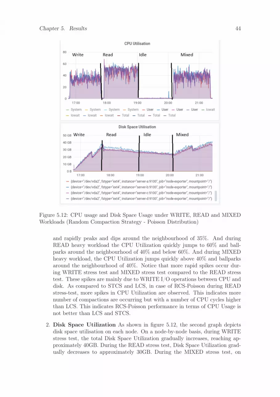
Chapter 5. Results 44
Figure 5.12: CPU usage and Disk Space Usage under WRITE, READ and MIXEDWorkloads (Random Compaction Strategy - Poisson Distribution)
and rapidly peaks and dips around the neighbourhood of 35%. And duringREAD heavy workload the CPU Utilization quickly jumps to 60% and ball-parks around the neighbourhood of 40% and below 60%. And during MIXEDheavy workload, the CPU Utilization jumps quickly above 40% and ballparksaround the neighbourhood of 40%. Notice that more rapid spikes occur dur-ing WRITE stress test and MIXED stress test compared to the READ stresstest. These spikes are mainly due to WRITE I/O operations between CPU anddisk. As compared to STCS and LCS, in case of RCS-Poisson during READstress-test, more spikes in CPU Utilization are observed. This indicates morenumber of compactions are occurring but with a number of CPU cycles higherthan LCS. This indicates RCS-Poisson performance in terms of CPU Usage isnot better than LCS and STCS.
2. Disk Space Utilization As shown in figure 5.12, the second graph depictsdisk space utilisation on each node. On a node-by-node basis, during WRITEstress test, the total Disk Space Utilization gradually increases, reaching ap-proximately 40GB. During the READ stress test, Disk Space Utilization grad-ually decreases to approximately 30GB. During the MIXED stress test, on

Chapter 5. Results 45
a node-by-node basis, the disk space utilization gradually increased, reachingabove 40GB. Compared to STCS, the disk space usage during WRITE stress-test is less, which indicates the size of SSTables generated by RCS-Poisson issmall compared to STCS. Notice that during READ stress test, the disk spaceutilization is rapidly altering, which indicates the disk space is being altereddue to compactions taking place during a READ operation. Notice that al-tering the disk space during each workload is very small, which indicates alarge number of SSTables have been generated. Compared to STCS and LCS,more number of spikes are occurring during each stress test which indicatesmore number of compactions are occurring, but the CPU Utilization by thisstrategy is higher compared to LCS, STCS and RCS-Uniform.
Random Compaction Strategy - Geometric Distribution
centring
Figure 5.13: CPU usage and Disk Space Usage under WRITE, READ and MIXEDWorkloads (Random Compaction Strategy - Geometric Distribution)
1. CPU UtilizationAs shown in figure 5.13,the first graph depicts CPU Utilisa-tion by Apache Cassandra application on each node. On a node-to-node basis,during WRITE stress test, the CPU Utilization jumps immediately to 37%and rapidly peaks and dips around the neighbourhood of 35%. And duringREAD heavy workload the CPU Utilization quickly jumps to 40% and ball-parks around the neighbourhood of 40% and below 60%. And during MIXED

Chapter 5. Results 46
heavy workload, the CPU Utilization jumps quickly above 40% and ballparksaround the neighbourhood of 40%. Notice that more rapid spikes occur dur-ing WRITE stress test and MIXED stress test compared to the READ stresstest. These spikes are mainly due to WRITE I/O operations between CPUand disk. As compared to STCS and LCS, in case of RCS-Geometric duringREAD stress-test more spikes in CPU Utilization are observed. This indicatesmore number of compactions occur with the number of CPU cycles lower thanLCS strategy’s number of CPU Cycles. This indicates RCS-Geometric perfor-mance in terms of CPU Usage is better than LCS, STCS, RCS-Uniform, andRCS-Poisson.
2. Disk Space UtilizationAs shown in figure 5.13, the second graph depicts diskspace utilisation on each node. On a node-by-node basis, during WRITE stresstest, the total Disk Space Utilization gradually increases, reaching approxi-mately 38GB. During READ stress test, the Disk Space Utilization graduallydecreases to approximately 10GB. During MIXED stress test, on a node-by-node basis, the disk space utilization peaks and dips around the neighbourhoodof 20GB. Compared to STCS, the disk space usage during WRITE stress-testis less, which indicates the size of SSTables generated by RCS-Geometric issmall compared to STCS. Notice that during READ stress test the disk spaceutilization is rapidly altering which indicates the disk space is being altered dueto occurrence of compactions. . Compared to STCS and LCS, more numberof spikes are occurring during each stress test which indicates more number ofcompactions are occurring, but the CPU Utilization by this strategy is lowercompared to LCS, STCS and RCS-Uniform and RCS-Poisson.
Descriptive Statistics - CPU Utilization
The values tabulated below are summary statistics computed using Microsoft Ex-cel by feeding the raw data recorded during stress testing by different exporters.The node exporter records the System Level metrics and exposes the metrics toPrometheus, and similarly, Cassandra Exporter exposes the metrics to Prometheus.There is not support of downloading raw data stored in Prometheus data storage.Grafana supports this downloading of raw data of metrics. These values representCPU Utilization in terms of percentages. This value is recorded every 15s. Thelesser the utilization of CPU during a heavy workload on application of compactionstrategy the higher will be the performance of the strategy in long run.
Strategy Total number of data points Average CPU Usage Std.Dev.STCS 249 31.51 8.12LCS 249 31.95 8.14
RCS-Uniform 249 31.98 8.08RCS-Poisson 249 32.38 6.91
RCS-Geometric 249 31.56 7.2
Table 5.8: Summary Statistics - CPU Usage under WRITE heavy workload on ap-plication of different compaction strategies

Chapter 5. Results 47
Strategy Total number of data points Average CPU Usage Std.Dev.STCS 219 43.5 7.81LCS 219 39.03 8.52
RCS-Uniform 219 34.70 7.26RCS-Poisson 219 43.79 13.68
RCS-Geometric 219 33.48 6.73
Table 5.9: Summary Statistics - CPU Usage under READ heavy workload on appli-cation of different compaction strategies
Strategy Total number of data points Average CPU Usage Std.Dev.STCS 256 37.60 10.23LCS 256 35.55 11.71
RCS-Uniform 256 35.16 6.39RCS-Poisson 256 35.43 8.91
RCS-Geometric 256 28.44 6.24
Table 5.10: Summary Statistics - CPU Usage under MIXED heavy workload onapplication of different compaction strategies
A graph using values noted in tables 5.8 - 5.10 is generated to depict the averageCPU usage under different workloads. From figure 5.14 the following observationsare drawn:
1. During WRITE heavy workload CPU Utilisation by each compaction strategyis similar.
2. During READ heavy workload RCS-Geometric has least CPU Utilization com-pared to other strategies. And RCS-Poisson has the highest CPU Utilizationamong all strategies.
3. During MIXED heavy workload RCS-Geometric has least CPU Utilizationcompared to other strategies.
Statistical Test (One-way ANOVA):
Null Hypothesis: CPU Utilization using STCS, LCS, RCS-Uniform, RCS-Poisson,RCS-Geometric strategies respectively are same under the workload performed.H0 : μSTCS = μLCS = μRCS−Uniform = μRCS−Poisson = μRCS−Geometric
Confidence Interval: 95%Dependent Variables: CPU UtilizationIndependent Variable: Compaction StrategyAlternate Hypothesis: CPU Utilization using STCS, LCS, RCS-Uniform, RCS-Poisson, RCS-Geometric strategies respectively are not same under the workloadperformed.H0 : μSTCS �= μLCS �= μRCS−Uniform �= μRCS−Poisson �= μRCS−Geometric
As per the values noted in table 5.11, the p-value for both READ and MIXEDworkloads is 0, the null hypothesis for these workloads is rejected which mean there

Chapter 5. Results 48
Figure 5.14: Comparison of Average CPU Utilisation under different heavy workloads
Workload p-valueWrite 0.71(>0.05)Read 0(<0.05)Mixed 0(<0.05)
Table 5.11: One Way ANOVA Test for CPU Utilization
is a significant difference in terms of CPU Usage among compaction strategies dur-ing READ and WRITE workloads. The p-value for WRITE workload is 0.71, sothe alternate hypothesis is rejected, which mean there is no significant difference interms of CPU Usage among different compaction strategies.
5.2.3 Cassandra Performance Metric - Operation Latency
Operation Latency: This metric describes the response time for completing anyoperation. This metric is measured in microseconds(μs).
1. Write Latency: The response time for completing a write request.
2. Read Latency: The response time for completing a read request.
Descriptive Statistics - Operation Latency
The values tabulated below are summary statistics of operation latency under READand WRITE workloads on Applying different compaction strategies.
A graph using values noted in tables 5.12 - 5.13 is generated to depict the writeoperation latency and read operation latency under WRITE and READ workloadsrespectively. From figure 5.15 following conclusions are drawn:
1. During WRITE stress-test RCS-Geometric has least mean operation latencyamong all strategies.
2. During READ stress-test STCS has least mean operation latency among allstrategies.

Chapter 5. Results 49
Strategy Total number of data points Mean Operation LatencySTCS 245 132LCS 245 127
RCS-Uniform 245 114RCS-Poisson 245 114
RCS-Geometric 245 91
Table 5.12: Summary Statistics - Operation Latency under WRITE heavy workloadon application of different compaction strategies
Strategy Total number of data points Mean Operation LatencySTCS 176 353LCS 176 411
RCS-Uniform 176 395RCS-Poisson 176 411
RCS-Geometric 176 462
Table 5.13: Summary Statistics - Operation Latency under READ heavy workloadon application of different compaction strategies
Figure 5.15: Operation Latency
Note that as the virtual machines used in building the cluster are memory-intensiveand highly powerful, the operation latency does not play a major role for comparingthe performances of the compaction strategies.

Chapter 6Discussion
6.1 Answers to Research Questions
6.1.1 RQ1: How a compaction strategy can be developed insuch a way the compaction strategy compacts a randomnumber of SSTables
A: The method administered to design and develop a random compaction strategyis discussed in chapter 4. The resultant implementation of stable random com-paction strategy is depicted in chapter 5. This random compaction strategy is im-plemented from scratch in two stages of development. To reduce space amplificationfile_splitting_chance is added to the strategy which breaks the created SSTable issplit into small SSTables. A random threshold generator module is integrated intothe code base of strategy. The compaction strategy uses this module to generate arandom threshold in which this random threshold serves as the number of SSTablesto be compacted. The random threshold generator module consists of different ran-dom number generating functions. Each function can generate a random thresholdbased upon the input probability distribution. To check if the performance can beimproved if the random threshold is generated from probability distribution otherUniform distribution, random threshold generator module is added to the strategy.
6.1.2 RQ2: How the performance of developed random com-paction strategy can be evaluated
A: The method administered to evaluate the performance of developed random com-paction strategy is discussed in chapter 4. As per the suggestions by a supervisor atEricsson and advisor at BTH, most important performance metrics are consideredfor evaluation. The random compaction strategy’s performance can be evaluated bycomparing the strategy’s performance with other strategies’ performance based onperformance metrics collected. These performance metrics include Operating Systemperformance metrics, such as CPU Utilization and Disk Space Utilization. These per-formance metrics include Cassandra Application performance metrics such as LiveSSTables, SSTables Per READ, Operation Latency. As discussed in chapter 5, interms of CPU Utilization, a number of Live SSTables and number of SSTables PerREAD, RCS-Uniform is performing better than LCS and STCS. In the case of STCS,a small number of large-sized SSTables are created after compactions. As the size ofSSTables is large, this can lead to space amplification problem. Due to the large size
50

Chapter 6. Discussion 51
of SSTables and the small number of SSTables existing on the disk, SSTables PerREAD is higher in the case of STCS. In the case of LCS, the SSTables are groupedinto levels. And the size of each SSTable is fixed. The last level contains most of thedata. As most of the data is in a single level, SSTables Per READ is reduced to 1indicating high performance. As the size of SSTables is small, compaction requiresa low space amplification. In the case of RCS, in the long run, the size of SSTablesgradually decreases; in parallel, the number of SSTables also gradually increases.This is due to file splitting after every compaction. The number of SSTables createdafter every compaction depends on the random threshold. The generation of randomthreshold pattern depends on Probability Distribution. From the results, we can ob-serve RCS-Uniform’s performance is almost similar to LCS and higher than STCS.And the performance of RCS-Geometric strategy is almost similar to STCS and lessthan RCS-Uniform strategy. From the results, we can observe RCS-Poisson’s per-formance is not better than RCS-Uniform, LCS and STCS. As per the pattern ofPoisson distribution, the random threshold generated always lies around the range of[0,10]. So, always a low number of SSTables are compacted each time a compactionis triggered. After compaction, the created SSTable is split into a small number ofSSTables, gradually accumulating a medium-sized, large number of SSTables.
6.2 Threats to ValidityThis section discusses the Validity of threats. The threats are classified as internalValidity and conclusion validity, as mentioned by Wohlin and Rohenson[30].
6.2.1 Internal Validity
Internal Validity refers to the influence of factors on research, which may affect thevalidation of results[30]. The threat can be a collection of performance metrics usingcustom scripts. If the performance metrics using simple tools such as JMX exporterthe data obtained can consist of false data. To overcome this threat, reputed opensource tools such as Prometheus and Grafana are used to collect the performancemetrics over certain time intervals.
6.2.2 Conclusion Validity
Conclusion Validity refers to whether the conclusions obtained from the experimentare true and justified [30]. The potential threat to this project is analyzing the resultsbased upon just the visualizations provided by Grafana. To overcome this threat, OneWay ANOVA Statistical test is done among the strategies with performance metricas the continuous dependent variable. Through this testing, it can be concludedwhether there is a statistically significant difference among the strategies.
6.3 Limitations1. Lack of Resources due to COVID-19: Due to unexpected pandemic situ-
ation the resources provided at Ericsson are not completely utilised.

Chapter 6. Discussion 52
2. No Better APIs provided by Grafana: Recently a new feature is releasedin Grafana. Using this new feature, the raw data can be downloaded in theform of CSV. Even though this feature is an excellent addition to Grafana, butthe data collected for the experiment is huge. Nearly 105 CSV data files havebeen downloaded to analyze the data. If the APIs provided by Grafana is muchbetter, then I would have drawn much better visualizations from Grafana.

Chapter 7Conclusions and Future Work
7.1 ConclusionsIn this thesis, an in-depth literature review is initially conducted to understandApache Cassandra API, Compaction Strategies APIs and limitations of the genericcompaction strategies Size Tiered Compaction strategy and Leveled CompactionStrategy studied. After studying Size Tiered Compaction Strategy’s limitations, theSize Tiered Compaction Strategy has a major limitation called High Space Amplifi-cation. In the past, to avoid this problem IT administrators at TelecommunicationIndustries and other IT industries used to horizontally scale the hard disks attachedto Cassandra Cluster’s nodes. After studying Leveled Compaction Strategy’s lim-itations, it is found the Leveled Compaction Strategy is having a major limitationcalled Write Amplification problem. As per this limitation, the data is written morethan once. And as the write operations are directly related to reading operations,the database’s READ performance is also affected. There is no particular solutionto this problem to write amplification. Even though Leveled Compaction Strategyis having a major problem of Write Amplification, the READ performance of Lev-eled Compaction Strategy is very high. Most of the Telecommunication Industriesuses Leveled Compaction Strategy for READ heavy workloads. To avoid both theproblems of high space amplification and high write amplification, a new compactionstrategy should be developed. This thesis focuses on the design and development ofa new compaction strategy which is an attempt to avoid these problems. This com-paction strategy uses the properties of randomness and compacts a random numberof SSTables. To reduce space amplification, file splitting feature is added to thestrategy. Using this feature, after compaction, the created SSTable is split into smallSSTables. To reduce CPU cycles wastage, a compaction chance parameter is addedto the strategy. This parameter decides whether the compaction should occur or not.This feature is added to the strategy to limit unnecessary compactions.
To check if the random compaction strategy’s performance can be altered by therandom threshold generation pattern, a random threshold generator module is addedto the strategy. This module consists of different random threshold generating func-tions. The threshold can be generated from different probability distributions.
Focus meetings with Ericsson’s CIL team and supervisor at BTH are conductedto gain insight knowledge of compaction strategies of Apache Cassandra and differ-ent APIs. After considering suggestions from a supervisor at BTH and supervisor
53

Chapter 7. Conclusions and Future Work 54
at Ericsson, only the most interesting and important performance metrics are con-sidered for evaluating Random Compaction Strategy’s performance. These metricsinclude Operating System performance metrics and Cassandra Application perfor-mance metrics. CPU Utilization and Disk Space Utilization are included in Operat-ing System performance metrics. A number of Live SSTables, Number of SSTablesPer READ and Operation Latency are included in Cassandra performance metrics.All these metrics are directly related to each other. To simulate the different stress-tests, a 4-node private Cassandra Cluster is built. This entire network of virtualmachines, including virtual simulator machine, is deployed on top of IBM Virtual Pri-vate Cloud Gen2. Compaction strategies STCS, LCS, RCS-Uniform, RCS-Poisson,RCS-Geometric, are stressed underwrite, read, mixed heavy workloads. From the re-sults, it is clearly observed that RCS-Uniform is performing better than LCS underboth READ heavy and MIXED heavy workloads. The SSTables Per READ in thecase of RCS-Uniform is also equal to 1 similar to LCS, which indicates a high READperformance. RCS-Poisson is not performing better than any other strategy duringall workloads. RCS-Geometric is performing better than STCS, but haven’t reachedthe performance of LCS during READ heavy and MIXED heavy workloads. TheRCS artefact is highly standardized. The write amplification problem encounteredin the case of LCS is not encountered in the case of RCS-Uniform. The problemsencountered in STCS and LCS are not encountered in the case of RCS.
Compared to all strategies, it can be concluded that RCS-Uniform strategy’s perfor-mance is high and almost similar to the performance of LCS. Furthermore, no spaceamplification problem and write amplification problem are encountered on the ap-plication of RCS. Moreover, the developed RCS uses by default Uniform distributionto generate the random threshold.
7.2 Future WorkIn the past, HDD has been used to store the SSTable data files. But recently, dueto advancements in technologies, SSD is being used to store the SSTable data files.Though SSD devices are faster in performance than HDD, the performance of SizeTiered Compaction and Leveled, Compaction Strategy is not efficiently improvedwhile using SSD. In this thesis, SSD disks are used to store the SSTable data files.The effects of the performance of compaction strategies on HDD and SSD can be ofgreat interest.In this thesis, the random number is generated from discrete probability distributionwhere this number indicates the number of SSTables to be compacted. A randomnumber can be generated from a discrete uniform probability distribution, discretePoisson probability distribution, discrete Geometric probability distribution. Butto tune the compaction strategy’s performance, other random number generatingfunctions can be integrated into the random number generator module.

Bibliography
[1] S. R. Alapati, Expert Apache Cassandra Administration, 1st ed. Berkeley, CA:Apress L. P, 2017;2018;.
[2] S. Bang, “Size tiered compaction strategy in apache cassandra |shrikant bang’s notes,” https://shrikantbang.wordpress.com/2014/04/22/size-tiered-compaction-strategy-in-apache-cassandra/, (Accessed on01/10/2021).
[3] A. Bonifati, P. K. Chrysanthis, A. M. Ouksel, and K.-U. Sattler,“Distributed databases and peer-to-peer databases: Past and present,”SIGMOD Rec., vol. 37, no. 1, p. 5–11, Mar. 2008. [Online]. Available:https://doi-org.miman.bib.bth.se/10.1145/1374780.1374781
[4] R. Bruno and P. Ferreira, “A study on garbage collection algorithms for bigdata environments,” ACM Comput. Surv., vol. 51, no. 1, Jan. 2018. [Online].Available: https://doi-org.miman.bib.bth.se/10.1145/3156818
[5] E. Capriolo, Cassandra High Performance Cookbook, 1st ed. Birmingham:Packt Publishing, Limited, 2011.
[6] F. Chang, J. Dean, S. Ghemawat, W. C. Hsieh, D. A. Wallach, M. Burrows,T. Chandra, A. Fikes, and R. E. Gruber, “Bigtable: A distributed storage systemfor structured data,” ACM transactions on computer systems, vol. 26, no. 2, pp.1–26, 2008.
[7] J.-K. Chen and W.-Z. Lee, “An introduction of nosql databases based on theircategories and application industries,” Algorithms, vol. 12, no. 5, p. 106, 2019.
[8] Datastax, “Architecture in brief | apache cassandra 3.x,” https://docs.datastax.com/en/cassandra-oss/3.x/cassandra/architecture/archIntro.html, (Accessedon 01/10/2021).
[9] M. Ghosh, I. Gupta, S. Gupta, and N. Kumar, “Fast compaction algorithms fornosql databases.” IEEE, 2015, pp. 452–461.
[10] Grafana, “Getting started | grafana labs,” https://grafana.com/docs/grafana/latest/getting-started/#what-is-grafana, (Accessed on 01/10/2021).
[11] IBM, “Ibm cloud docs,” https://cloud.ibm.com/docs/vpc?topic=vpc-getting-started, (Accessed on 01/10/2021).
[12] C. Y. Kan, Cassandra data modeling and analysis: design, build, and analyzeyour data intricately using Cassandra, 1st ed. PACKT Publishing, 2014.
[13] R. R. KATIKI REDDY, “Improving efficiency of data compaction by creating& evaluating a random compaction strategy in apache cassandra,” Master’sthesis, , Department of Software Engineering, 2020.
55

BIBLIOGRAPHY 56
[14] S. Kona, “Compactions in apache cassandra : Performance analysis of com-paction strategies in apache cassandra,” 2016.
[15] A. LAKSHMAN and P. MALIK, “Cassandra - a decentralized structured storagesystem,” Operating systems review, vol. 44, no. 2, pp. 35–40, 2010.
[16] L. M. Lix, J. C. Keselman, and H. J. Keselman, “Consequences of assumptionviolations revisited: A quantitative review of alternatives to the one-way analysisof variance "f" test,” Review of educational research, vol. 66, no. 4, pp. 579–619,1996.
[17] B. Lu and Y. Xiaohui, “Research on cassandra data compaction strategies fortime-series data,” Journal of computers, vol. 11, no. 6, pp. 504–512, 2016.
[18] M. D. MacLaren, “The art of computer programming. volume 2: Seminumericalalgorithms,” pp. 306–308, 1970.
[19] A. Mahgoub, S. Ganesh, F. Meyer, A. Grama, and S. Chaterji, “Suitability ofnosql systems — cassandra and scylladb — for iot workloads.” Piscataway:The Institute of Electrical and Electronics Engineers, Inc. (IEEE), 2017, p. 476.
[20] P. Otterström, “Github - eperott/cassandra-exporter: Java agent forexporting cassandra metrics to prometheus,” https://github.com/eperott/cassandra-exporter, (Accessed on 01/10/2021).
[21] A. Paez, “Gray literature: An important resource in systematic reviews,” Jour-nal of evidence-based medicine, vol. 10, no. 3, pp. 233–240, 2017.
[22] S. Pi, “Establish the cornerstone of big data: Nosql database technique,” inTopTeam Information Co., Ltd., 2016.
[23] J. Pokorny, “Nosql databases: a step to database scalability in web environ-ment.” ACM, 2011, pp. 278–283.
[24] Prometheus, “Monitoring linux host metrics with the node exporter |prometheus,” https://prometheus.io/docs/guides/node-exporter/, (Accessed on01/10/2021).
[25] W. Puangsaijai and S. Puntheeranurak, “A comparative study of relationaldatabase and key-value database for big data applications,” in 2017 Interna-tional Electrical Engineering Congress (iEECON), 2017, pp. 1–4.
[26] P. Raj and G. Deka, A Deep Dive into NoSQL Databases: The Use Cases andApplications, 1st ed. Academic Press, 2018, vol. 109, ch. 1.
[27] V. S. S. J. S. Ravu, “Compaction strategies in apache cassandra : Analysis ofdefault cassandra stress model,” 2016.
[28] Scylladb, “Choose a compaction strategy | scylla docs,” https://docs.scylladb.com/architecture/compaction/compaction-strategies/, (Accessed on01/10/2021).
[29] N. Serrano, G. Gallardo, and J. Hernantes, “Infrastructure as a service and cloudtechnologies,” IEEE Software, vol. 32, no. 2, pp. 30–36, 2015.
[30] C. Wohlin, P. Runeson, M. Höst, M. C. Ohlsson, B. Regnell, and A. Wesslén,Experimentation in software engineering, 2012th ed. Berlin: Springer, 2012,vol. 9783642290442.

BIBLIOGRAPHY 57
[31] S. Yarabarla, Learning Apache Cassandra - Second Edition, 2nd ed. PacktPublishing, 2017.

Appendix ASupplemental Information
58


Faculty of Engineering, Blekinge Institute of Technology, 371 79 Karlskrona, Sweden