controls structure interaction on the jupiter icy moons orbiter

Acta Astronautica 65 (2009) 766–786www.elsevier.com/locate/actaastro

Controls structure interaction on the Jupiter IcyMoonsOrbiter

Marco B. Quadrellia,∗, Edward Mettlera, Don Solowayb, Atul Kelkarc

aMail Stop 198-326, Guidance and Control Analysis Group, Jet Propulsion Laboratory, California Institute of Technology, 4800 Oak GroveDrive, Pasadena, CA 91109-8099, USA

bNASA Ames Research Center, M/S 269-3, Moffett Field, CA 94035, USAcMechanical & Aerospace Engineering Department, 2018 Black, Iowa State University, Ames, IA 50011, USA

Received 28 March 2007; accepted 5 March 2009Available online 26 May 2009

Abstract

The baseline Jupiter Icy Moons Orbiter (JIMO) spacecraft presented challenging controls–structure interactions caused byhaving to accurately and simultaneously point the existing multiple articulated payloads (high-gain antenna, scan platform) whichare mounted on a large flexible base. Sensitivity analyses and simulation studies were carried out using complex finite elementmodels describing the vehicle’s dynamics. The results of these studies indicate that: (1) the attitude controller bandwidth (BW)should be less than 0.01Hz for stable pointing control at the end of a slew with fine thrusters; (2) to achieve a 90◦ slew maneuverin 2h the attitude controller BW should be greater than 0.0001Hz with coarse thrusters; and (3) the first natural frequencyof the flexible vehicle should be in the range of 1Hz, to avoid potential interactions with other flexible modes. A dissipativecontroller ensures the stability robustness during large-angle maneuvers of the articulated payloads at high speeds when linearityassumptions are likely to be incorrect and nonlinearity in dynamics may be significant. An advantage of the proposed controlleris that the closed-loop stability is not only robust to unmodeled dynamics but also to actuator nonlinearities as expected in theproposed gimbals for JIMO.© 2008 Elsevier Ltd. All rights reserved.

Keywords: Spacecraft dynamics; Flexible spacecraft; Attitude control; Pointing

1. Introduction

NASA developed early plans for an ambitious mis-sion to orbit three planet sized moons of Jupiter—Callisto, Ganymede and Europa—which may harborvast liquid oceans beneath their icy surfaces. The objec-tive of the JIMO (Jupiter Icy Moons Orbiter) missionstudy was to design a spacecraft to explore the threeicy moons and investigate their makeup, their historyand their potential for sustaining life. To do so, NASA

∗Corresponding author.E-mail address: [email protected]

(M.B. Quadrelli).

0094-5765/$ - see front matter © 2008 Elsevier Ltd. All rights reserved.doi:10.1016/j.actaastro.2009.03.013

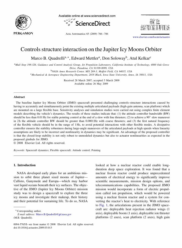
looked at how a nuclear reactor could enable long-duration deep space exploration. It was found that anuclear fission reactor could produce unprecedentedamounts of electrical energy to significantly improvescientific measurements, mission design options, andtelecommunications capabilities. The proposed JIMOmission would incorporate a form of electric propul-sion called ion propulsion, which would be poweredusing a nuclear fission reactor and a system for con-verting the reactor’s heat to electricity. With referenceto Fig. 1, the articulations present in the JIMO space-craft are: deployable heat rejection radiator wings (1axis), deployable boom (1 axis), deployable ion thrusterplatforms (2 axes), scan platform (2 axes), high gain

http://www.elsevier.com/locate/actaastro

mailto:[email protected]

M.B. Quadrelli et al. / Acta Astronautica 65 (2009) 766–786 767

DeployableReactor Boom

DeployableReactor Heat Rejection

Radiator Wings

DeployableRadiators

DeployableMagnetometer Boom

Deployable Scan Platform

Deployable Ion ThrusterPlatforms

Deployable Telecom Platform

DeployableFields & Particles

Platform

Deployable Solar Arrays

Fig. 1. The proposed Jupiter Icy Moons Orbiter.

and medium gain antennas (2 axes), turntable (1 axis),deployable magnetometer boom (1 axis), deployable so-lar arrays (2 axes), and optical navigation camera (2axes). The large number of articulated platforms makesthe JIMO spacecraft a truly complex flexible multibodysystem. It is the intent of this paper to model some ofthe interactions of these articulations with the rest ofthe vehicle, and point out their interactions with the at-titude control system during pointing.For the JIMO spacecraft, it is a near certainty that

structure modes would lie within the various controlsystem bandwidths (BWs) or near cross-over regions.High-Q model resonances would not be rolled-offenough to prevent amplitude response above 0dB andwill threaten gain stabilized closed loop stability in thethrust vector controller and scan platform pointing sta-bility. Since large center of mass migration would existwith xenon usage over the mission, global structuremodes would change and any control filters would berendered useless or destabilizing unless re-tuned basedon in-flight system identification (ID) periodically totrack changes. The means for system ID depends onadequate excitation actuators, special input designs,and sensitive low frequency dynamic accelerometers.Transient inputs do not suffice, and a capability for lowfrequency sine sweep and dwell requires proof-massactuators (PMA) that would reveal both the local andglobal structure modes. Modal analysis of the articula-

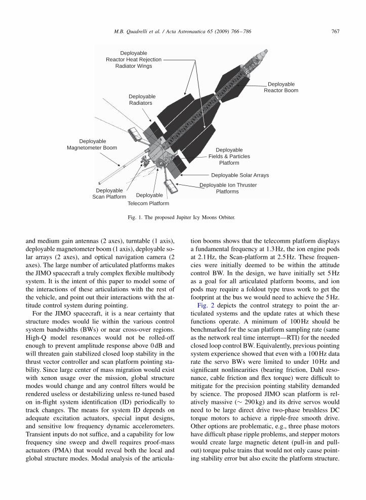
tion booms shows that the telecomm platform displaysa fundamental frequency at 1.3Hz, the ion engine podsat 2.1Hz, the Scan-platform at 2.5Hz. These frequen-cies were initially deemed to be within the attitudecontrol BW. In the design, we have initially set 5Hzas a goal for all articulated platform booms, and ionpods may require a foldout type truss work to get thefootprint at the bus we would need to achieve the 5Hz.Fig. 2 depicts the control strategy to point the ar-

ticulated systems and the update rates at which thesefunctions operate. A minimum of 100Hz should bebenchmarked for the scan platform sampling rate (sameas the network real time interrupt—RTI) for the neededclosed loop control BW. Equivalently, previous pointingsystem experience showed that even with a 100Hz datarate the servo BWs were limited to under 10Hz andsignificant nonlinearities (bearing friction, Dahl reso-nance, cable friction and flex torque) were difficult tomitigate for the precision pointing stability demandedby science. The proposed JIMO scan platform is rel-atively massive (∼ 290kg) and its drive servos wouldneed to be large direct drive two-phase brushless DCtorque motors to achieve a ripple-free smooth drive.Other options are problematic, e.g., three phase motorshave difficult phase ripple problems, and stepper motorswould create large magnetic detent (pull-in and pull-out) torque pulse trains that would not only cause point-ing stability error but also excite the platform structure.

768 M.B. Quadrelli et al. / Acta Astronautica 65 (2009) 766–786

After describing the equations of motion of the rigidspacecraft in orbit, the model of the flexible spacecraftalone and of the flexible spacecraft with multiple rigidpayloads is described. Next, we identify some featuresof the interaction between the flexible spacecraft dy-namics and the pointing control loops, and quantify thisinteraction in nondimensional form as a function of con-troller type. The controls–structure interaction (CSI) isthen analyzed in simulation by varying the structuralfrequency and the controller frequency during a slewmaneuver, and the results of the simulations with andwithout flexibility are discussed.

2. Spacecraft equations of motion

The equations of motion of the entire system will bederived in this section. We introduce [1] the Europa-centric inertial reference frame �I , X pointing towardthe vernal equinox, Z toward the North Pole, and Ycompletes the right handed reference frame, and the or-biting reference frame �ORF, which we use to describethe near field dynamics of the spacecraft relative to its

Scan PlatformAttitude Controller

HGA Attitude Commander

HGA Attitude Determination

Scan Platform Attitude

Commander

Basebody Attitude Commander

HGA Attitude Controller

Thrusters

HGA ActuatorsGimbal

Actuators

Gyros

Star Tracker

Gyros

Star Tracker

SunSens

Scan Platform SID/ Attitude Estimator

Encoders

Encoders

BasebodyAttitude Controller

EP GimbalDrives

10 hz 100 hz

10 hz

BasebodyH/W

Scan Plat H/W

S/W Functions

Rate groups

Solar Array

Encoder

Solar Array Gimbal

Controller

Solar Array Drive

Basebody Star Identification (SID)/ Attitude Estimator

RCS Thrust Vector Controller

Accels

EPEncoders

EP Thrust Vector Controller

Inertial Vector Propagator

Fig. 2. Articulated systems control strategy.

orbit. This reference frame is attached to a point thatfollows a Keplerian orbit around the primary body.The body-fixed reference frame is defined as: the y-body directed from the bus towards the reactor, thex-body axis directed from the bus toward the right-most ion engine pod, the z-body axis completes theright-handed triad. The motion of the system is de-scribed with respect to a local vertical–local horizontal(LV–LH) orbiting reference frame (x, y, z) = �ORF oforigin OORF which rotates with mean motion � andorbital semi-major axis R0, z along the local vertical,x toward the flight direction, and y in the orbit normaldirection. When the spacecraft’s attitude is displacedfrom the attitude of the �ORF frame, the pitch angle isdefined as the angle between the body-fixed y- and thez-axis in the plane of the orbit, the yaw angle is de-fined as the out-of-plane angle between the body-fixedy-axis and orbit plane, and the roll axis is defined asthe angle around the body-fixed y-axis. The orbit ofthe origin of �ORF, point OORF, is propagated forwardin time under the influence of the gravitational field ofEuropa. The position vector of a generic structural point


with respect to OORF is denoted by qi , and we haveri =R0 +qi . We define the state vector as X= (R0, V0,q1, q1, v1,x1, . . . , qN , qN , vN ,xN ,�w1, �w2, �w3, �w1,�w2, �w3)T . The translation kinematics and dynamicsequations of a point mass of mass m in a general orbitare

q= −R0 − X× q−X×X× q− 2X× q+ r

(near field) (1)

r = −�Er

|r|3 + fa + fs + f3m

(far field) (2)

R0 = − �E

|R30 |R0 + fpert + fJ2 + fJ3

m

(ORF orbital dynamics) (3)

where q is the relative position vector of mass withrespect to ORF, R0 the orbital radius vector to ori-gin of ORF, X the orbital rate, �E the Jupiter moongravitational parameter, fa the thruster actuation forcevector, fs the solar pressure force vector, f3 the

third-body forces vector, m the spacecraft mass withrotors added, and fpert , fJ2 , fJ3 the resultants of higherorder gravitational terms from the primary acting on theentire system as an extended body. Eqs. (1–3) describesthe Keplerian orbital dynamics. The rotational dynamicsequations of a spacecraft with a gyroscopic distributionabout its center of mass are

Jx+∑i

Hwi + x× (Jx+

∑i

Hwi ) = ge + ga (4)

Hwi = −gwi (i = 1, . . . , number of rotors) (5)

where x is the spacecraft’s body angular rate, ge the ex-ternal perturbation torques (solar pressure, gravity gra-dient, J2, etc.), ga the thruster actuator torques, gw therotor control torque, J the spacecraft moment of inertia,Hw

i the angular momentum of the i th rotor.The equations of motion for the flexible spacecraft

in global coordinates can be written in terms of theconfiguration vector q (of length ng+1), which containsthe nodal displacements and rotations of each node inglobal coordinates plus the rotor rotation angles plus

the rigid body degrees of freedom. The global equationsneed to be reduced from the global set ng of dependentconfiguration variables to a set of independent degreesof freedom ne, and this is done by a transformationq = Tqe, where T is of dimension ng × ne. Splittingthe equations in elastic (e) and rigid (r) coordinates, wehave

Meeqe + Mer X+ (Gee + Dee)qe + Keeqe = fe

Mreqe + Mrr X= fr (6)

where now Mee = TTMgT, and similarly for the othermatrices. Assuming small base body angular rates (sothat the nonlinear coupling terms are negligible, and themodes are still the mass-normalized undamped modes),and introducing K as the diagonal matrix of natural fre-quencies, and � as the modal damping coefficient, wecan impose the modal transformation qe = Dg, whereD is the modal matrix. Introducing the state vectoras x = (g, b, g,X)T , where � represents the rotor an-gles (reaction wheel, Brayton’s turbine), the state spacemodel takes the following form:

x =

⎛⎜⎝

��

⎞⎟⎠=

[ 0 I

−[

I DTMew

MewD Mww

]−1 [DT (Gee + Dee)D 00 0

]−[

I DTMew

MewD Mww

]−1 [K2 00 0

]]⎛⎜⎝

��

⎞⎟⎠

+⎡⎣ 0

−[

I DTMew

MewD Mww

]−1 [DT 00 I

]⎤⎦(feefw

)= Ax + Bu (7)

where D is the modal matrix, K the matrix of naturalfrequencies (diagonal),Mew the modal inertia matrix ofcoupling of deformation degrees of freedom with rotordegrees of freedom, Mww the rotor inertia matrix, Gee

the gyroscopic coupling matrix, Dee the modal dampingmatrix, fee the external forces on boom nodes (includesthruster and reactor control forces), fw the torques onrotors.

3. Equations of motion of rigid appendage on rigidbase

To derive the equations of motion of the multiplepayload system, we used a projection method, whichcombines Kane’s derivation of generalized speeds [2]with Hughes’ vectrix approach [3]. We now assume thatthe generic platform and the base body are rigid bodiesmoving in space. We denote by I the inertial referenceframe, by B the base body (spacecraft), and by P the ar-ticulated body. Each body is represented by a rigidly at-tached basis (vectrix, in matrix representation) denotedby Fk , where k = I, B, P , respectively, for each body.


B+

P+H

H

O

FI

FB

FP

λ1

λ2c

h

d

τ2

f1

f2

τ1

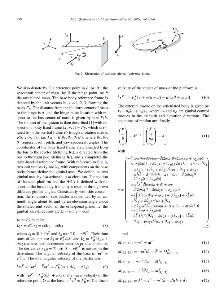
Fig. 3. Kinematics of two-axis gimbal (universal joint).

We also denote by O a reference point in B, by B+ thespacecraft center of mass, by H the hinge point, by Pthe articulated mass. The base body reference frame isdenoted by the unit vectors bi , i = 1, 2, 3, forming thebasis FB . The distance from the platform center of massto the hinge is d, and the hinge point location with re-spect to the bus center of mass is given by h = Fbh.The motion of the system is then described [1] with re-spect to a body fixed frame (x, y, z)= FB , which is ro-tated from the inertial frame FI trough a rotation matrixR(�1, �2, �3), i.e. FB = R(�1, �2, �3)FI , where �1, �2,�3 represent roll, pitch, and yaw spacecraft angles. Thecoordinates of the body fixed frame are z directed fromthe bus to the reactor (defining b3), x directed from thebus to the right pod (defining b1), and y completes theright-handed reference frame. With reference to Fig. 3,two unit vectors k1 and k2, with components on the basebody frame, define the gimbal axes. We define the twogimbal axes by � = azimuth, = elevation. The motionof the scan platform and the HGA is defined with re-spect to the base body frame by a rotation through twodifferent gimbal angles. Consistently with this conven-tion, the rotation of one platform is defined by an az-imuth angle about b2 and by an elevation angle aboutthe rotated unit vector in the orthogonal plane, i.e. thegimbal axis directions are (s= sin, c= cos)

k1 = FTB �1 = b2

k2s = FTB �2 = c�b1 − s�b3 (8)

where �1= (0 1 0)T and �2= (c� 0 −s�)T . Their timerates of change are k1 = FT

B ��1 and k2 = FTB (�2,� +

��2), where the tilde denotes the cross-product operator.The derivative �2,� = �(−s� 0 − c�)T is needed in thederivation. The angular velocity of the base is IxB =FTB �. The total angular velocity of the platform is

IxP = IxB + BxP = FTB (� + ��1 + �2) (9)

with BxP = FTB (��1 + �2). The linear velocity of the

reference point O at the base is IvO = FTB v. The linear

velocity of the center of mass of the platform is

IvP+ = FT

B [v + �(h + d) − d(�1� + �2)] (10)

The external torque on the articulated body is given bys2 = n�k1 + nk2, where n� and n� are gimbal controltorques in the azimuth and elevation directions. Theequations of motion are, finally,⎛⎜⎝

v

��

⎞⎟⎠= M−1

⎡⎢⎣⎛⎜⎝

f1 1n�n

⎞⎟⎠− �

⎤⎥⎦ (11)

with

� =

⎛⎜⎜⎜⎜⎜⎜⎜⎜⎜⎜⎜⎜⎜⎜⎜⎜⎜⎜⎜⎜⎜⎜⎜⎜⎝

m2[��(h+d)+�v−d(2��1�+2��2 + �2,�)]

×J2[�(��1+�2)+�2,�]+�(J1�+J2(�+��1+�2)) + (��1 + �2)J2(� + ��1 + �2)+m2(h + d)[��(h + d) + �v − d(2��1�+2��2 + �2,�)]

×m2�T1 d[��(h + d) + �v

−d(2��1� + 2��2 + �2,�)]

+�T1 J2[�(��1 + �2) + �2,�] + �T1 (�

+��1 + �2)J2(� + ��1+�2)m2�T2 d[��(h + d) + �v − d(2��1�+2��2 + �2,�)]

+�T2 J2[�(��1 + �2) + �2,�] + �T2 (�

+��1 + �2)J2(� + ��1 + �2)

⎞⎟⎟⎟⎟⎟⎟⎟⎟⎟⎟⎟⎟⎟⎟⎟⎟⎟⎟⎟⎟⎟⎟⎟⎟⎠

(12)

and

M(1:3,1:3) = m1 + m2 (13)

M(1:3,4:6) = −m2(h + d) = MT(4:6,1:3) (14)

M(1:3,7) = −m2d�1 = MT(7,1:3) (15)

M(1:3,8) = −m2d�2 = MT(8,1:3) (16)

M(4:6,4:6) = J 1 + J 2 − m2(h + d)(h + d) (17)


M(4:6,7) = [J 2 − m2(h + d)d]�1 = MT(7,4:6) (18)

M(4:6,8) = [J 2 − m2(h + d)d]�2 = MT(8,4:6) (19)

M(7,7) = −�T1 [J2 + m2dd]�1 (20)

M(8,8) = −�T2 [J2 + m2dd]�2 (21)

These equations must be augmented with the Euler pa-rameter kinematics equations, describing the base bodyattitude parameterization, as follows:

˙� = 12 (� × � + �4�)

�4 = − 12�

T � (22)

where (aT , a4)T is the vector of Euler parameters forthe base body. � is the vector of the first three ele-ments of unit quaternion � defined as � = (�1, �2, �3)T ,�4 = cos(�/2) is the unit vector along the eigen-axisof rotation, and � is the magnitude of the rotation. Thequaternion is subject to the norm constraint �T �+�24=1.The measured outputs are the Euler parameters and an-gular velocity for the base body and relative angulardisplacement and rate for the appendage body.

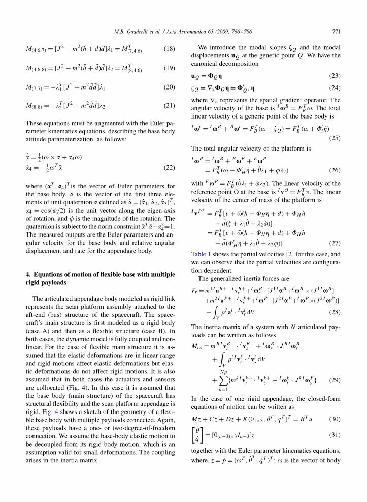
4. Equations of motion of flexible base with multiplerigid payloads

The articulated appendage body modeled as rigid linkrepresents the scan platform assembly attached to theaft-end (bus) structure of the spacecraft. The space-craft’s main structure is first modeled as a rigid body(case A) and then as a flexible structure (case B). Inboth cases, the dynamic model is fully coupled and non-linear. For the case of flexible main structure it is as-sumed that the elastic deformations are in linear rangeand rigid motions affect elastic deformations but elas-tic deformations do not affect rigid motions. It is alsoassumed that in both cases the actuators and sensorsare collocated (Fig. 4). In this case it is assumed thatthe base body (main structure) of the spacecraft hasstructural flexibility and the scan platform appendage isrigid. Fig. 4 shows a sketch of the geometry of a flexi-ble base body with multiple payloads connected. Again,these payloads have a one- or two-degree-of-freedomconnection. We assume the base-body elastic motion tobe decoupled from its rigid body motion, which is anassumption valid for small deformations. The couplingarises in the inertia matrix.

We introduce the modal slopes fQ and the modaldisplacements uQ at the generic point Q. We have thecanonical decomposition

uQ =UQg (23)

�Q = ∇xUQg=U′Q, g (24)

where ∇x represents the spatial gradient operator. Theangular velocity of the base is IxB = FT

B �. The totallinear velocity of a generic point of the base body is

Ixi = IxB + Bxi = FTB (� + �Q) = FT

B (� + �′i )

(25)

The total angular velocity of the platform is

IxP = IxB + BxE + ExP

= FTB (� + �′

H + ��1 + �2) (26)

with ExP = FTB (��1 + �2). The linear velocity of the

reference point O at the base is IvO = FTB v. The linear

velocity of the center of mass of the platform is

IvP+ = FT

B [v + �(h + �H + d) + �H

− d(� + �1� + �2)]

= FTB [v + �(h + �H + d) + �H

− d(�′H + �1� + �2)] (27)

Table 1 shows the partial velocities [2] for this case, andwe can observe that the partial velocities are configura-tion dependent.The generalized inertia forces are

Fr = m1 I aB+ · I vB+r +IxB

r · [J1 IaB+IxB × (J1 IxB ]

+m2 I aP+ · I vP+r +IxP · [J2 IaP+IxP×(J2 IxP )]

+∫V

�I ai · I vir dV (28)

The inertia matrix of a system with N articulated pay-loads can be written as follows

Mrs = mB IvB+r · IvB+

s + IxBr · J B IxB

s

+∫V

�i Ivir · Ivis dV

+Np∑k=1

{mk Ivk+r · Ivk+s + Ixkr · J k IxPs } (29)

In the case of one rigid appendage, the closed-formequations of motion can be written as

Mz + Cz + Dz + K (01×3, �T , qT )T = BT u (30)[

�q

]= [0(n−3)×3 In−3]z (31)

together with the Euler parameter kinematics equations,

where, z= p = (�T , �T, qT )T ; � is the vector of body


B+

P+

H

H

FI

FB

FP

h

d

τ2

τ1

f1

f2

u

λ1

λ2

O

c

Fig. 4. Flexible base with attached payload.

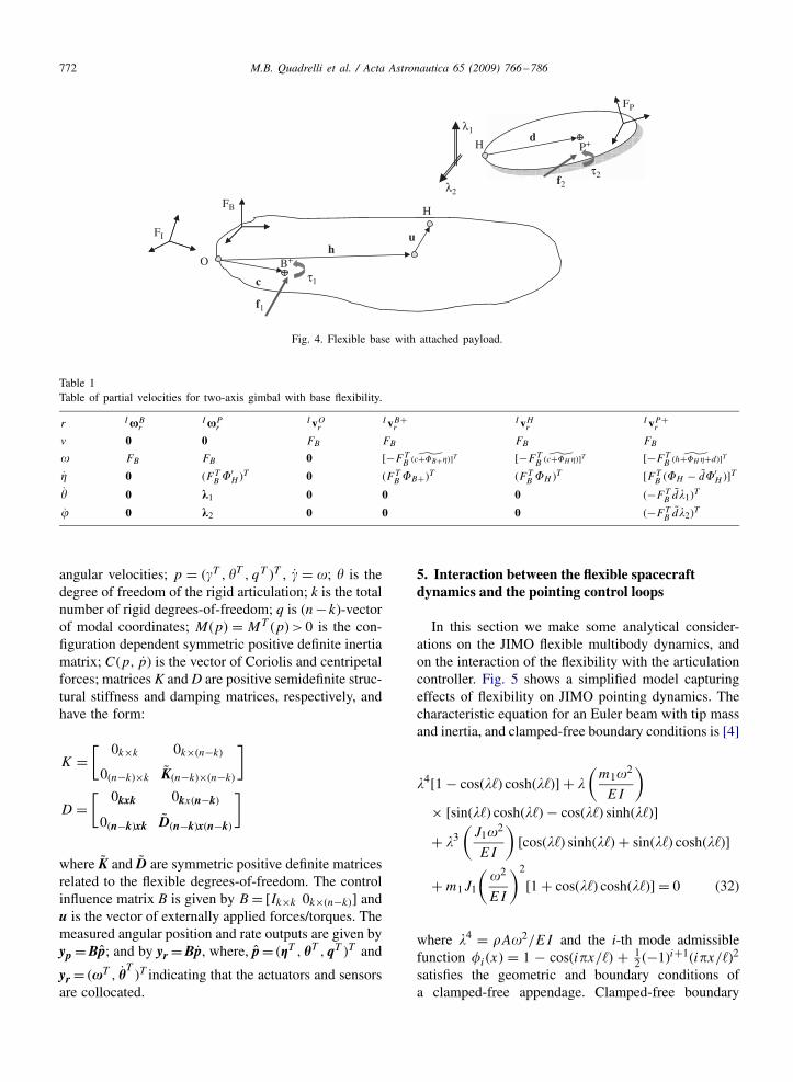
Table 1Table of partial velocities for two-axis gimbal with base flexibility.

r IxBr

IxPr

I vOrI vB+

rI vHr

I vP+r

v 0 0 FB FB FB FB

� FB FB 0 [−FTB

˜(c+�B+)]T [−FTB

˜(c+�H )]T [−FTB

˜(h+�H +d)]T

0 (FTB �′

H )T 0 (FT

B �B+)T (FTB �H )T [FT

B (�H − d�′H )]

T

� 0 k1 0 0 0 (−FTB d�1)T

0 k2 0 0 0 (−FTB d�2)T

angular velocities; p = (�T , �T , qT )T , � = �; � is thedegree of freedom of the rigid articulation; k is the totalnumber of rigid degrees-of-freedom; q is (n− k)-vectorof modal coordinates; M(p) = MT (p)> 0 is the con-figuration dependent symmetric positive definite inertiamatrix; C(p, p) is the vector of Coriolis and centripetalforces; matrices K and D are positive semidefinite struc-tural stiffness and damping matrices, respectively, andhave the form:

K =[ 0k×k 0k×(n−k)

0(n−k)×k K(n−k)×(n−k)

]

D =[ 0kxk 0kx(n−k)

0(n−k)xk D(n−k)x(n−k)

]

where K and D are symmetric positive definite matricesrelated to the flexible degrees-of-freedom. The controlinfluence matrix B is given by B = [Ik×k 0k×(n−k)] andu is the vector of externally applied forces/torques. Themeasured angular position and rate outputs are given byyp =Bp; and by yr =Bp, where, p= (gT , hT , qT )T and

yr = (xT , hT)T indicating that the actuators and sensors

are collocated.

5. Interaction between the flexible spacecraftdynamics and the pointing control loops

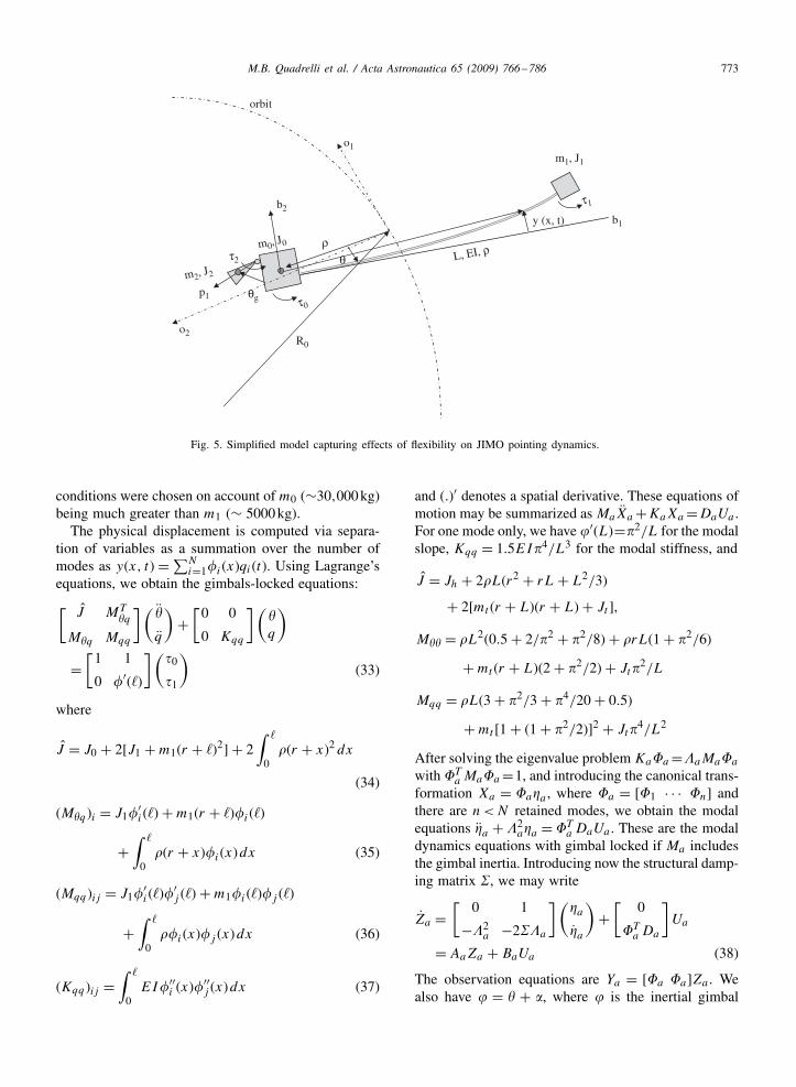
In this section we make some analytical consider-ations on the JIMO flexible multibody dynamics, andon the interaction of the flexibility with the articulationcontroller. Fig. 5 shows a simplified model capturingeffects of flexibility on JIMO pointing dynamics. Thecharacteristic equation for an Euler beam with tip massand inertia, and clamped-free boundary conditions is [4]

�4[1 − cos(��) cosh(��)] + �

(m1�2

E I

)× [sin(��) cosh(��) − cos(��) sinh(��)]

+ �3(J1�2

E I

)[cos(��) sinh(��) + sin(��) cosh(��)]

+ m1 J1

(�2

E I

)2

[1 + cos(��) cosh(��)] = 0 (32)

where �4 = �A�2/E I and the i-th mode admissiblefunction �i (x) = 1 − cos(i�x/�) + 1

2 (−1)i+1(i�x/�)2

satisfies the geometric and boundary conditions ofa clamped-free appendage. Clamped-free boundary


m1, J1

m0, J0

L, EI, ρ

τ0

y (x, t)

θ

o2

o1

b1

orbit

τ2

θgp1

b2

ρ

R0

τ1

m2, J2

Fig. 5. Simplified model capturing effects of flexibility on JIMO pointing dynamics.

conditions were chosen on account of m0 (∼30,000kg)being much greater than m1 (∼ 5000kg).

The physical displacement is computed via separa-tion of variables as a summation over the number ofmodes as y(x, t) =∑N

i=1�i (x)qi (t). Using Lagrange’sequations, we obtain the gimbals-locked equations:[ J MT

�q

M�q Mqq

](�

q

)+[0 0

0 Kqq

](�q

)

=[1 1

0 �′(�)

]( 0

1

)(33)

where

J = J0 + 2[J1 + m1(r + �)2] + 2∫

�

0�(r + x)2 dx

(34)

(M�q )i = J1�′i (�) + m1(r + �)�i (�)

+∫

�

0�(r + x)�i (x)dx (35)

(Mqq )i j = J1�′i (�)�

′j (�) + m1�i (�)� j (�)

+∫

�

0��i (x)� j (x)dx (36)

(Kqq )i j =∫

�

0E I�′′

i (x)�′′j (x)dx (37)

and (.)′ denotes a spatial derivative. These equations ofmotion may be summarized as Ma Xa +KaXa =DaUa .For one mode only, we have ′(L)=�2/L for the modalslope, Kqq = 1.5E I�4/L3 for the modal stiffness, and

J = Jh + 2�L(r2 + r L + L2/3)

+ 2[mt (r + L)(r + L) + Jt ],

M�� = �L2(0.5 + 2/�2 + �2/8) + �r L(1 + �2/6)

+ mt (r + L)(2 + �2/2) + Jt�2/L

Mqq = �L(3 + �2/3 + �4/20 + 0.5)

+ mt [1 + (1 + �2/2)]2 + Jt�4/L2

After solving the eigenvalue problem Ka�a =�aMa�a

with �Ta Ma�a =1, and introducing the canonical trans-

formation Xa = �aa , where �a = [�1 · · · �n] andthere are n < N retained modes, we obtain the modalequations a + �2

aa = �Ta DaUa . These are the modal

dynamics equations with gimbal locked if Ma includesthe gimbal inertia. Introducing now the structural damp-ing matrix �, we may write

Za =[

0 1

−�2a −2��a

](aa

)+[

0

�Ta Da

]Ua

= Aa Za + BaUa (38)

The observation equations are Ya = [�a �a]Za . Wealso have = � + �, where is the inertial gimbal


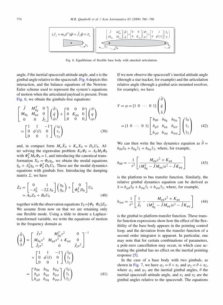
Fig. 6. Equilibrium of flexible base body with attached articulation.

angle, � the inertial spacecraft attitude angle, and � is thegimbal angle relative to the spacecraft. Fig. 6 depicts thisinteraction, and the balance equations of the Newton-Euler scheme used to represent the system’s equationsof motion when the articulated payload is present. FromFig. 6, we obtain the gimbals-free equations:

⎡⎣ J MT

�q 0M�q Mqq 0

0 0 J2

⎤⎦( �

q

)+[0 0 00 Kqq 00 0 0

]( �q

)

=[1 1 −10 �′(�) 00 0 1

]( 0 1 2

)(39)

and, in compact form Ma Xb + KaXb = DaUb. Af-ter solving the eigenvalue problem Kb�b = �bMb�b

with �Tb Mb�b=1, and introducing the canonical trans-

formation Xb = �bb, we obtain the modal equationsb + �2

bb = �Tb DbUb. These are the modal dynamics

equations with gimbals free. Introducing the dampingmatrix �, we have

Zb =[

0 1−�2

b −2��b

](bb

)+[

0�Tb Db

]Ub

= AbZb + BbUb (40)

together with the observation equations Yb=[�b �b]Zb.We assume from now on that we are retaining onlyone flexible mode. Using a tilde to denote a Laplace-transformed variable, we write the equations of motionin the frequency domain as

( �q�

)=⎡⎣ J s2 MT

�qs2 0

M�qs2 Mqqs2 + Kqq 0

J2s2 0 J2s2

⎤⎦

−1

×[1 1 −10 �′(�) 00 0 1

]( 0 1 2

)

=[ b�� b�q b�bq� bqq bqb� bq b

]( 0 1 2

)(41)

If we now observe the spacecraft’s inertial attitude angle(through a star tracker, for example) and the articulationrelative angle (through a gimbal-axis mounted resolver,for example), we have

Y = = [1 0 · · · 0 1]

⎛⎜⎝

�

q

�

⎞⎟⎠

= [1 0 · · · 0 1]

⎡⎢⎣b�� b�q b�

bq� bqq bq

b� bq b

⎤⎥⎦⎛⎜⎝

0

1

2

⎞⎟⎠ (42)

We can then write the bus dynamics equation as � =b�� 0 + b�q 1 + b� 2, where, for example,

b�� = − 1

s2

[Mqqs2 + Kqq

(M2�q − J Mqq )s2 − J Kqq

](43)

is the platform to bus transfer function. Similarly, therelative gimbal dynamics equation can be derived as� = b� 0 + bq 1 + b 2, where, for example,

b = 1

s2

[1

J2− Mqqs2 + Kqq

(M2�q − J Mqq )s2 − J Kqq

](44)

is the gimbal to platform transfer function. These trans-fer function expressions show how the effect of the flex-ibility of the base body appears in the pointing controlloop, and the deviation from the transfer function of asecond order integrator is apparent. In particular, onemay note that for certain combinations of parameters,a pole-zero cancellation may occur, in which case ac-tuating the gimbal has no effect on the inertial pointingresponse [5].In the case of a base body with two gimbals, as

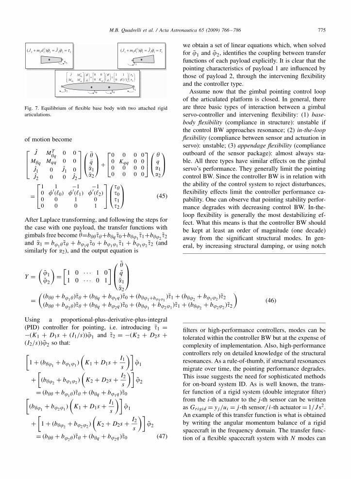
shown in Fig. 7, we have 1 = � + �1 and 2 = � + �2,where 1 and 2 are the inertial gimbal angles, � theinertial spacecraft attitude angle, and �1 and �2 are thegimbal angles relative to the spacecraft. The equations


Fig. 7. Equilibrium of flexible base body with two attached rigidarticulations.

of motion become

⎡⎢⎢⎣

J MT�q 0 0

M�q Mqq 0 0

J1 0 J1 0J2 0 0 J2

⎤⎥⎥⎦⎛⎜⎝

�q�1�2

⎞⎟⎠+

⎡⎢⎣0 0 0 00 Kqq 0 00 0 0 00 0 0 0

⎤⎥⎦⎛⎜⎝

�q�1�2

⎞⎟⎠

=

⎡⎢⎣1 1 −1 −10 �′(�0) �′(�1) �′(�2)0 0 1 00 0 0 1

⎤⎥⎦⎛⎜⎝

� 0 1 2

⎞⎟⎠ (45)

After Laplace transforming, and following the steps forthe case with one payload, the transfer functions withgimbals free become �=b�� +b�q 0+b�1

1+b�2 2

and �1 = b1� � + b1q 0 + b11 1 + b12

2 (andsimilarly for �2), and the output equation is

Y =(

12

)=[1 0 · · · 1 01 0 · · · 0 1

]⎛⎜⎝�q�1�2

⎞⎟⎠

=((b�� + b1�) � + (b�q + b1q ) 0 + (b�1+b11

) 1 + (b�2+ b12

) 2(b�� + b2�) � + (b�q + b2q ) 0 + (b�1

+ b21) 1 + (b�2

+ b22) 2

)(46)

Using a proportional-plus-derivative-plus-integral(PID) controller for pointing, i.e. introducing 1 =−(K1 + D1s + (I1/s))1 and 2 = −(K2 + D2s +(I2/s))2 so that:

[1 + (b�1

+ b11)

(K1 + D1s + I1

s

)]1

+[(b�2

+ b12)

(K2 + D2s + I2

s

)]2

= (b�� + b1�) � + (b�q + b1q ) 0[(b�1

+ b21)

(K1 + D1s + I1

s

)]1

+[1 + (b�2

+ b22)

(K2 + D2s + I2

s

)]2

= (b�� + b2�) � + (b�q + b2q ) 0 (47)

we obtain a set of linear equations which, when solvedfor 1 and 2, identifies the coupling between transferfunctions of each payload explicitly. It is clear that thepointing characteristics of payload 1 are influenced bythose of payload 2, through the intervening flexibilityand the controller type.Assume now that the gimbal pointing control loop

of the articulated platform is closed. In general, thereare three basic types of interaction between a gimbalservo-controller and intervening flexibility: (1) base-body flexibility (compliance in structure): unstable ifthe control BW approaches resonance; (2) in-the-loopflexibility (compliance between sensor and actuation inservo): unstable; (3) appendage flexibility (complianceoutboard of the sensor package): almost always sta-ble. All three types have similar effects on the gimbalservo’s performance. They generally limit the pointingcontrol BW. Since the controller BW is in relation withthe ability of the control system to reject disturbances,flexibility effects limit the controller performance ca-pability. One can observe that pointing stability perfor-mance degrades with decreasing control BW. In-the-loop flexibility is generally the most destabilizing ef-fect. What this means is that the controller BW shouldbe kept at least an order of magnitude (one decade)away from the significant structural modes. In gen-eral, by increasing structural damping, or using notch

filters or high-performance controllers, modes can betolerated within the controller BW but at the expense ofcomplexity of implementation. Also, high-performancecontrollers rely on detailed knowledge of the structuralresonances. As a rule-of-thumb, if structural resonancesmigrate over time, the pointing performance degrades.This issue suggests the need for sophisticated methodsfor on-board system ID. As is well known, the trans-fer function of a rigid system (double integrator filter)from the i-th actuator to the j-th sensor can be writtenas Grigid = y j/ui = j-th sensor/ i-th actuator= 1/J s2.An example of this transfer function is what is obtainedby writing the angular momentum balance of a rigidspacecraft in the frequency domain. The transfer func-tion of a flexible spacecraft system with N modes can


instead be written as

Grigid+ f lex = Grigid +N∑

k=1

(�i j )k

where �i j = (�ki �

kj/mk)/(s2 +2�k�ks+�2

k) is the con-tribution of one flexible mode. An example of this trans-fer function is representative of the attitude dynamicsof one spacecraft around one axis when a boom ap-pendage is present, and this is the case for JIMO asEqs. (43)–(44) clearly show.We conclude this section with some qualitative con-

siderations. Gain margin can be defined as the amountof gain of a closed-loop controlled system that can beincreased (decreased) before the system goes unstable.Phase margin can be defined as the amount of phasethat can be decreased (increased) before it goes unsta-ble. Phase margin affects the response of the closedloop system. In simple terms, the controller BW is ap-proximately the crossover frequency of the closed-looptransfer function. For a second order controlled struc-tural system with roll-off well above the flexible mode,the resonance is phase-stabilized, and gain and phasemargin are modest. For JIMO, if the controller BW iswell above flexible mode (i.e., closing the loop on thescan-platform while the base body in JIMO behaves asa noodle), there is still enough control authority for theplatform to not be disturbed by the base body and stilldo its pointing well. In the limit, the scan platform isa stand-alone body in free space, and the system canstill be pointed. For a second order structural systemwith roll-off well below the flexible mode, the reso-nance is gain-stabilized, and gain and phase margin arealso modest. For JIMO, if the controller BW is well be-low flexible mode (i.e., closing the loop on the JIMObase-body attitude while the Ion engine pod booms areflexing), the high frequency boom dynamics would nothave enough inertia to react to the control action, hencetheir effect on the attitude is minor, and the system canstill be pointed. For a second order structural systemwith roll-off in the vicinity of the flexible mode, neg-ative margins result since the gain margin is high nearthe phase crossover, and the phase margin is high nearthe gain crossover. This is the main reason why modalresonances have to be kept away from the controllerBW. For JIMO: if the controller BW is in the vicinityof a flexible mode (i.e., closing the loop on the scan-platform at a rate commensurate with one of the base-body frequencies), the stability margins are adverse, andthe system cannot be pointed. Additional complicationswould arise when the structural modes are clustered (in-stead of in alternate pole-zero pairs), or when additional

system modes of a different nature need to be included,such as sloshing modes.

6. Interaction between controller type and vehicleflexibility

In this section, a simplified qualitative analysis iscarried out following Ref. [6] to gain insight into thespacecraft-controller frequency separation. Although inreality discrete effects such as sampling rate and actu-ator and sensor saturation would limit the performanceof the closed-loop control system with flexibility, weidealize the plant by a system of two masses connectedvia a rotary spring and dashpot, and assume collocatedand ideal sensors and actuators. Consider then a simplesystem of two inertias I1 (spacecraft) and I2 (reactor)connected by some compliance. We also assume that thecompliance is known, and that gain stabilization is suffi-cient to stabilize the spacecraft. For JIMO, in the direc-tion of the largest moment of inertia (when the Xenonis totally depleted): I1=17e5kgm2, I2=3e5kgm2 andI1/I2 = 5.6667. The natural frequency is �2

n = k/I2,and the controller frequency is �2

c = kc/(I1 + I2). Theequations of motion are

I1�1 + 2��n I2(�1 − �2) + k(�1 − �2) = 1 + cI2�2 + 2��n I2(�2 − �1) + k(�2 − �1) = 2 (48)

Assume that the control law in the L-transform domainis of the form c = −kcH (s)�1, where H (s) is the con-troller transfer function yet to be specified, so that

�1 =[1 −

(I2s2

(I1 + I2)�2n

)(�2n

s2 + 2��ns + �2n

)

+�2c

s2H (s)

]−1 [ 1 + 2

(I1 + I2)s2−(

2(I1 + I2)�2

n

)

×(

�2n

s2 + 2��ns + �2n

)](49)

The characteristic equation is

1 −(

I2s2

(I1 + I2)�2n

)(�2n

s2 + 2��ns + �2n

)

+ �2c

s2H (s) = 0 (50)

In the vicinity of the resonant mode, for Nyquist-stability we need the fulfillment of the condition∣∣∣∣�2

c

�2nH ( j�n) − I2

2 j�(I1 + I2)

∣∣∣∣< 1


10−3 10−2 10−10

2

4

6

8

10

12

damping ratio

natu

ral f

requ

ency

/con

trol f

requ

ency

inertia ratio I1/I2 = 5.6667

r = flat gainb = 6 db/octave c = 12 db/octave

Fig. 8. Natural frequency/control frequency ratio vs. damping for fixed inertia ratio of 5.667.

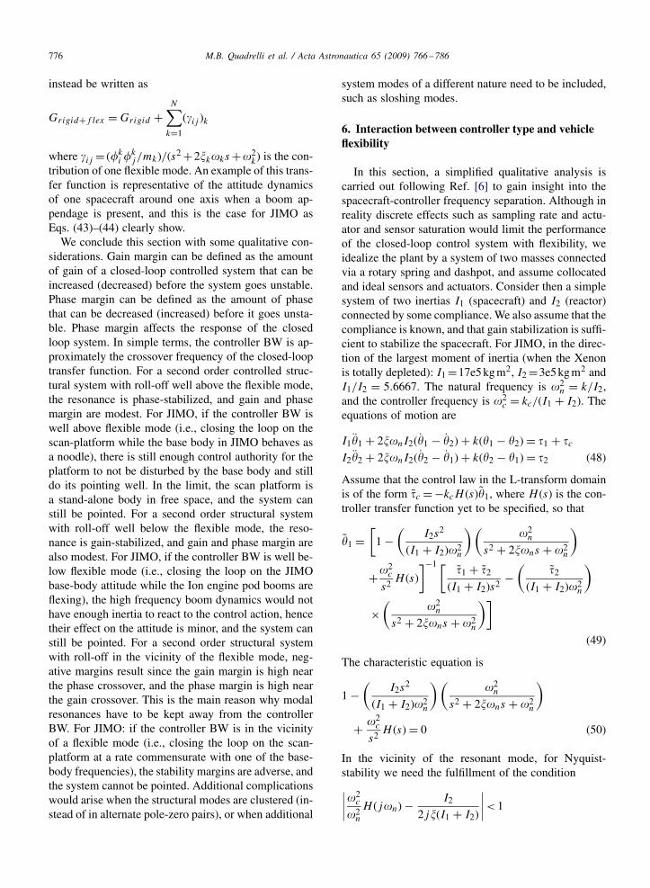
where |H ( j�n)|=(�c/�n)r for�> �c and |H ( j�n)|=1 for �< �c. Substituting, we obtain the equation forthe natural frequency/control frequency ratio as a func-tion of controller order

�n

�c>

⎧⎨⎩ I22�I1

(I1 + I2

I1

)−(3+r )/2

×[1 + 4�2

(I 21 + I 22I1 I2

)]1/2⎫⎬⎭

1/(2+r )

(51)

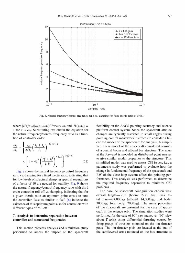
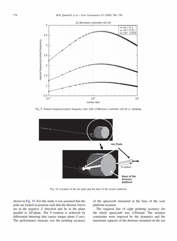
Fig. 8 shows the natural frequency/control frequencyratio vs. damping for a fixed inertia ratio, indicating thatfor low levels of structural damping spectral separationsof a factor of 10 are needed for stability. Fig. 9 showsthe natural frequency/control frequency ratio with thirdorder controller roll-off vs. damping, indicating that fora given inertia ratio an optimum point exists to tunethe controller. Results similar to Ref. [6] indicate theexistence of this optimum point also for controllers withdifferent types of roll-off.

7. Analysis to determine separation betweencontroller and structural frequencies

This section presents analysis and simulation studyperformed to assess the impact of the spacecraft

flexibility on the AACS pointing accuracy and scienceplatform control system. Since the spacecraft attitudechanges are typically restricted to small angles duringpointing control maneuvers it suffices to consider a lin-earized model of the spacecraft for analysis. A simpli-fied linear model of the spacecraft considered consistsof a central boom and aft-end bus structure. The massat the fore-end is modeled as distributed point massesto give similar modal properties to the structure. Thissimplified model was used to assess CSI issues, i.e., aparametric study was performed to evaluate how thechange in fundamental frequency of the spacecraft andBW of the close-loop system affect the pointing per-formance. This analysis was performed to determinethe required frequency separation to minimize CSIproblems.The baseline spacecraft configuration chosen was:

overall length—30m (boom: 27m; bus: 3m), to-tal mass—24,000kg (aft-end: 14,000kg; mid body:3000kg; fore body: 7000kg). The mass propertiesof the spacecraft are assumed for the case of space-craft in the science orbit. The simulation studies wereperformed for the case of 90◦ yaw maneuver (90◦ slewabout Y -axis) using differential thrusting caused byfiring group of thrusters mounted on the ion thrusterpods. The ion thruster pods are located at the end ofthe cantilevered arms mounted on the bus structure as


10−1 100 1010.5

1

1.5

2

2.5

3

3.5

4

inertia ratio

natu

ral f

requ

ency

/con

trol f

requ

ency

12 db/octave controller roll−off

csi = 0.1csi = 0.01csi= 0.001

Fig. 9. Natural frequency/control frequency ratio with 12dB/octave controller roll-off vs. damping.

Base of the Science platform

Ion Pods

6 meters

Fig. 10. Location of the ion pods and the base of the science platform.

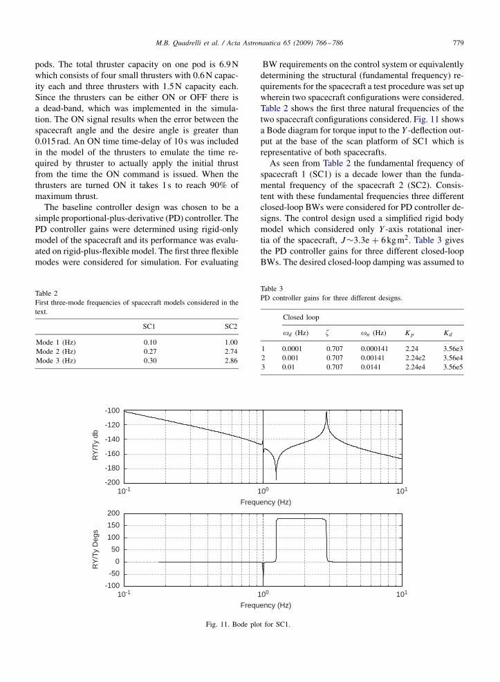
shown in Fig. 10. For this study it was assumed that thepods are locked in position such that the thruster forcesare in the negative Z direction and lie in the planeparallel to XZ-plane. The Y -rotation is achieved bydifferential thrusting that causes torque about Y -axis.The performance measure was the pointing accuracy

of the spacecraft measured at the base of the scanplatform location.The required line of sight pointing accuracy for

the whole spacecraft was ±20mrad. The actuatorconstraints were imposed by the dynamics and themaximum capacity of the thrusters mounted on the ion


pods. The total thruster capacity on one pod is 6.9Nwhich consists of four small thrusters with 0.6N capac-ity each and three thrusters with 1.5N capacity each.Since the thrusters can be either ON or OFF there isa dead-band, which was implemented in the simula-tion. The ON signal results when the error between thespacecraft angle and the desire angle is greater than0.015 rad. An ON time time-delay of 10s was includedin the model of the thrusters to emulate the time re-quired by thruster to actually apply the initial thrustfrom the time the ON command is issued. When thethrusters are turned ON it takes 1s to reach 90% ofmaximum thrust.The baseline controller design was chosen to be a

simple proportional-plus-derivative (PD) controller. ThePD controller gains were determined using rigid-onlymodel of the spacecraft and its performance was evalu-ated on rigid-plus-flexible model. The first three flexiblemodes were considered for simulation. For evaluating

Table 2First three-mode frequencies of spacecraft models considered in thetext.

SC1 SC2

Mode 1 (Hz) 0.10 1.00Mode 2 (Hz) 0.27 2.74Mode 3 (Hz) 0.30 2.86

10-1 100 101-200

-180

-160

-140

-120

-100

RY

/Ty

db

Frequency (Hz)

10-1 100 101

Frequency (Hz)

-100-50

050

100150200

RY

/Ty

Deg

s

Fig. 11. Bode plot for SC1.

BW requirements on the control system or equivalentlydetermining the structural (fundamental frequency) re-quirements for the spacecraft a test procedure was set upwherein two spacecraft configurations were considered.Table 2 shows the first three natural frequencies of thetwo spacecraft configurations considered. Fig. 11 showsa Bode diagram for torque input to the Y -deflection out-put at the base of the scan platform of SC1 which isrepresentative of both spacecrafts.As seen from Table 2 the fundamental frequency of

spacecraft 1 (SC1) is a decade lower than the funda-mental frequency of the spacecraft 2 (SC2). Consis-tent with these fundamental frequencies three differentclosed-loop BWs were considered for PD controller de-signs. The control design used a simplified rigid bodymodel which considered only Y -axis rotational iner-tia of the spacecraft, J∼3.3e + 6kgm2. Table 3 givesthe PD controller gains for three different closed-loopBWs. The desired closed-loop damping was assumed to

Table 3PD controller gains for three different designs.

Closed loop

�d (Hz) � �n (Hz) Kp Kd

1 0.0001 0.707 0.000141 2.24 3.56e32 0.001 0.707 0.00141 2.24e2 3.56e43 0.01 0.707 0.0141 2.24e4 3.56e5


0 20 40 60 80-10

-5

0

5

10

Fz (N

)

Time (min)

Tuned: 0.0001Hz

-20

-10

0

10

20

Y-E

rror

(mra

ds)

-1

-0.5

0

0.5

1 x 10-3

Y-Fl

ex (m

rads

)

0 20 40 60 80-10

-5

0

5

10

Fz (N

)

Time (min)

Tuned: 0.001Hz

-20

-10

0

10

20

Y-E

rror

(mra

ds)

-1

-0.5

0

0.5

1 x 10-3

Y-Fl

ex (m

rads

)

0 20 40 60 80-10

-5

0

5

10

Fz (N

)

Time (min)

0 20 40 60 80Time (min)

0 20 40 60 80Time (min)

0 20 40 60 80Time (min)

0 20 40 60 80Time (min)

0 20 40 60 80Time (min)

0 20 40 60 80Time (min)

Tuned: 0.01Hz

-200

-100

0

100

200

Y-E

rror

(mra

ds)

-1

-0.5

0

0.5

1 x 10-3

Y-Fl

ex (m

rads

)

Fig. 12. Step responses for SC2.

be 0.707 for optimal rise time. The thruster dynamicswas modeled fairly accurately to reflect its delay andrise time characteristics typical of ion engines.Two maneuvers were used to tests the control of the

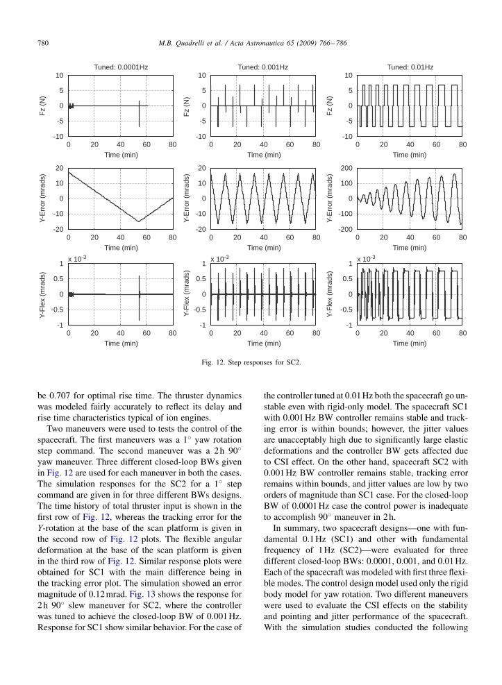
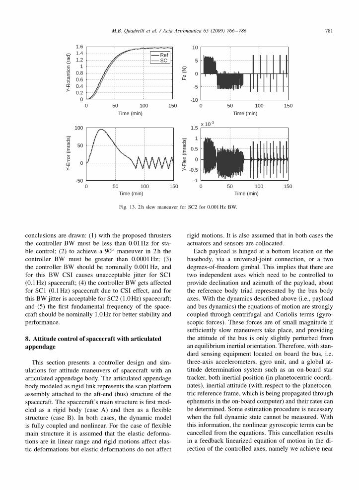
spacecraft. The first maneuvers was a 1◦ yaw rotationstep command. The second maneuver was a 2h 90◦yaw maneuver. Three different closed-loop BWs givenin Fig. 12 are used for each maneuver in both the cases.The simulation responses for the SC2 for a 1◦ stepcommand are given in for three different BWs designs.The time history of total thruster input is shown in thefirst row of Fig. 12, whereas the tracking error for theY-rotation at the base of the scan platform is given inthe second row of Fig. 12 plots. The flexible angulardeformation at the base of the scan platform is givenin the third row of Fig. 12. Similar response plots wereobtained for SC1 with the main difference being inthe tracking error plot. The simulation showed an errormagnitude of 0.12mrad. Fig. 13 shows the response for2h 90◦ slew maneuver for SC2, where the controllerwas tuned to achieve the closed-loop BW of 0.001Hz.Response for SC1 show similar behavior. For the case of

the controller tuned at 0.01Hz both the spacecraft go un-stable even with rigid-only model. The spacecraft SC1with 0.001Hz BW controller remains stable and track-ing error is within bounds; however, the jitter valuesare unacceptably high due to significantly large elasticdeformations and the controller BW gets affected dueto CSI effect. On the other hand, spacecraft SC2 with0.001Hz BW controller remains stable, tracking errorremains within bounds, and jitter values are low by twoorders of magnitude than SC1 case. For the closed-loopBW of 0.0001Hz case the control power is inadequateto accomplish 90◦ maneuver in 2h.In summary, two spacecraft designs—one with fun-

damental 0.1Hz (SC1) and other with fundamentalfrequency of 1Hz (SC2)—were evaluated for threedifferent closed-loop BWs: 0.0001, 0.001, and 0.01Hz.Each of the spacecraft was modeled with first three flexi-ble modes. The control design model used only the rigidbody model for yaw rotation. Two different maneuverswere used to evaluate the CSI effects on the stabilityand pointing and jitter performance of the spacecraft.With the simulation studies conducted the following


0 50 100 1500

0.20.40.60.8

11.21.41.6

Y-R

otan

tion

(rad

)

Time (min)0 50 100 150

-10

-5

0

5

10

Fz (N

)

Time (min)

0 50 100 150-50

0

50

100

Y-E

rror

(mra

ds)

Time (min)0 50 100 150

-1

-0.5

0

0.5

1

1.5x 10-3

Y-Fl

ex (m

rads

)

Time (min)

RefSC

Fig. 13. 2h slew maneuver for SC2 for 0.001Hz BW.

conclusions are drawn: (1) with the proposed thrustersthe controller BW must be less than 0.01Hz for sta-ble control; (2) to achieve a 90◦ maneuver in 2h thecontroller BW must be greater than 0.0001Hz; (3)the controller BW should be nominally 0.001Hz, andfor this BW CSI causes unacceptable jitter for SC1(0.1Hz) spacecraft; (4) the controller BW gets affectedfor SC1 (0.1Hz) spacecraft due to CSI effect, and forthis BW jitter is acceptable for SC2 (1.0Hz) spacecraft;and (5) the first fundamental frequency of the space-craft should be nominally 1.0Hz for better stability andperformance.

8. Attitude control of spacecraft with articulatedappendage

This section presents a controller design and sim-ulations for attitude maneuvers of spacecraft with anarticulated appendage body. The articulated appendagebody modeled as rigid link represents the scan platformassembly attached to the aft-end (bus) structure of thespacecraft. The spacecraft’s main structure is first mod-eled as a rigid body (case A) and then as a flexiblestructure (case B). In both cases, the dynamic modelis fully coupled and nonlinear. For the case of flexiblemain structure it is assumed that the elastic deforma-tions are in linear range and rigid motions affect elas-tic deformations but elastic deformations do not affect

rigid motions. It is also assumed that in both cases theactuators and sensors are collocated.Each payload is hinged at a bottom location on the

basebody, via a universal-joint connection, or a twodegrees-of-freedom gimbal. This implies that there aretwo independent axes which need to be controlled toprovide declination and azimuth of the payload, aboutthe reference body triad represented by the bus bodyaxes. With the dynamics described above (i.e., payloadand bus dynamics) the equations of motion are stronglycoupled through centrifugal and Coriolis terms (gyro-scopic forces). These forces are of small magnitude ifsufficiently slow maneuvers take place, and providingthe attitude of the bus is only slightly perturbed froman equilibrium inertial orientation. Therefore, with stan-dard sensing equipment located on board the bus, i.e.three-axis accelerometers, gyro unit, and a global at-titude determination system such as an on-board startracker, both inertial position (in planetocentric coordi-nates), inertial attitude (with respect to the planetocen-tric reference frame, which is being propagated throughephemeris in the on-board computer) and their rates canbe determined. Some estimation procedure is necessarywhen the full dynamic state cannot be measured. Withthis information, the nonlinear gyroscopic terms can becancelled from the equations. This cancellation resultsin a feedback linearized equation of motion in the di-rection of the controlled axes, namely we achieve near


perfect state decoupling, and we can design the localcontrollers assuming independent control loops. Thepointing control algorithms developed for this study relyon a feedback linearization of the dynamics to derivea globally, exponentially stable controller for the point-ing dynamics. An attitude estimator on board the busprovides real-time estimates of the attitude quaternionand angular velocity. A command profiler specifies thecommand to be tracked, in the form of a constant ora step vs. time. These commands are provided to thecontroller in the form of desired attitude, angular ve-locity, and angular acceleration. It is desired to cancelall possible dynamic nonlinearities arising from gyro-scopic and centrifugal terms, as derived from the equa-tions of motion. The rotational control torque vector sis then of the following form:

s= Cpi [k(�err)] + Cvi (NxP

Cmd − NxPEst)

+ JPNaPCmd + hcancel (52)

where Cpi and Cvi are rotational control gain matri-ces, JP is the payload moment of inertia matrix, k isthe unit eigenaxis of rotation, �err is the magnitude ofrotation corresponding to the difference between thecommanded ((·)Cmd) and the estimated ((·)Est) quater-nion, hcancel is the vector of the centrifugal and Coriolisnonlinear terms to be cancelled, which can be obtainedfrom the appropriate terms in the equation of motion,and NxP and NaP are the inertial angular velocity andacceleration vectors of the payload, respectively.As an extension of the control law shown in Eq. (52),

passivity-based controllers have been shown to be veryeffective [7] in control of large flexible space struc-tures. It was proved in [7] that passivity-based con-troller can robustly stabilize nonlinear multibody flexi-ble space system if the actuator sensors are collocated.The stability was also shown to be robust to certain ac-tuator sensor nonlinearities. In this JIMO design study,one of such controllers was used to simulate the closed-loop maneuvers of spacecraft using nonlinear dynamicsof the spacecraft. The assumptions made in this simu-lation study include the following: (1) actuator sensorsare collocated and (2) flexible dynamics of the structureis considered to be in linear range and dynamic cou-pling is only from rigid to flexible, i.e., rigid motionsexcite flexibility but flexible deflections do not affectrigid motion. This statement originates in the following:Stability Theorem5: The closed-loop system consist-

ing of Eqs. (30) and (31) and the nonlinear dissipativecontrol law given by

u = −Gpp − Gryr (53)

is asymptotically stable. A proof of the theorem is givenin Ref. [8]. In Eq. (53), p=(aT, h)T, yr is the rate output,and matrices Gp and Gr are symmetric positive definiteand Gp is given by

Gp = diag[ 12 {( ˜a+ I3�4)Gp1 + �(1 − �4)I3},Gp2]

where � is a positive scalar, ˜a represents a cross productoperator matrix (�x ), I3 is the 3× 3 identity matrix andGp1, Gp2 are 3×3 and 1×1 symmetric positive definitematrix, respectively.The simulation study presented here is for closed-

loop 90◦ yaw maneuver of the spacecraft for both casesA and B discussed above. The maneuver is performedover the period of 2h, which is representative of themaneuver in the science orbit where spacecraft needsre-orientation for pointing at the required target. Thenonlinear control law given in Eq. (53) was used toachieve this maneuver. The controller gains chosen bytrial and error to obtain a satisfactory performance areGp1 = diag[15000, 15000, 9000], Gp2 = 9000, Gr =diag[90000, 100000, 90000, 9000], � = 500000. Thesystematic synthesis procedure for selection of thesegains is not available and will be focus of future re-search. The simulation results for cases A and B are verysimilar as the elastic deformations are fairly small com-pared to the displacement magnitudes during the grossmaneuver. The flexibility does not cause any destabi-lizing effect under this control law. Since the articu-lated joint is assumed to be purely rigid (i.e., no jointflexibility) observation spillover due to rate sensor isavoided. Future work will address the issue of jointflexibility.In order to assess the CSI effect the 90◦ slew for yaw

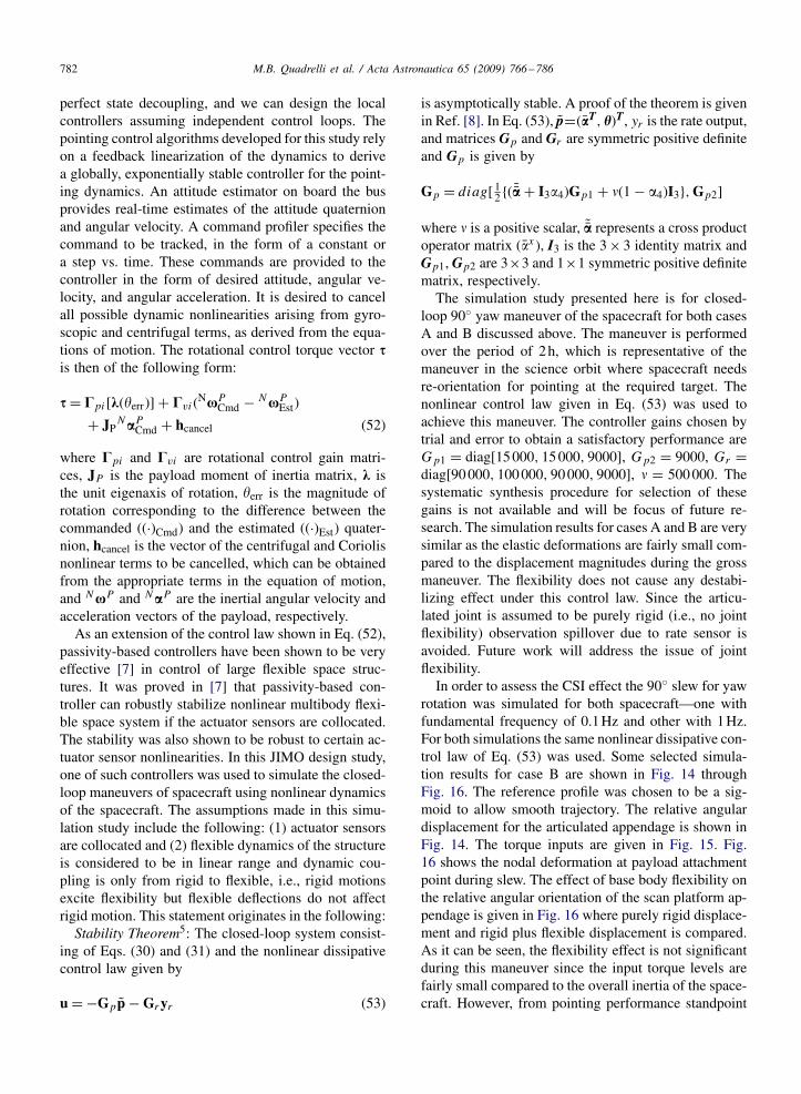
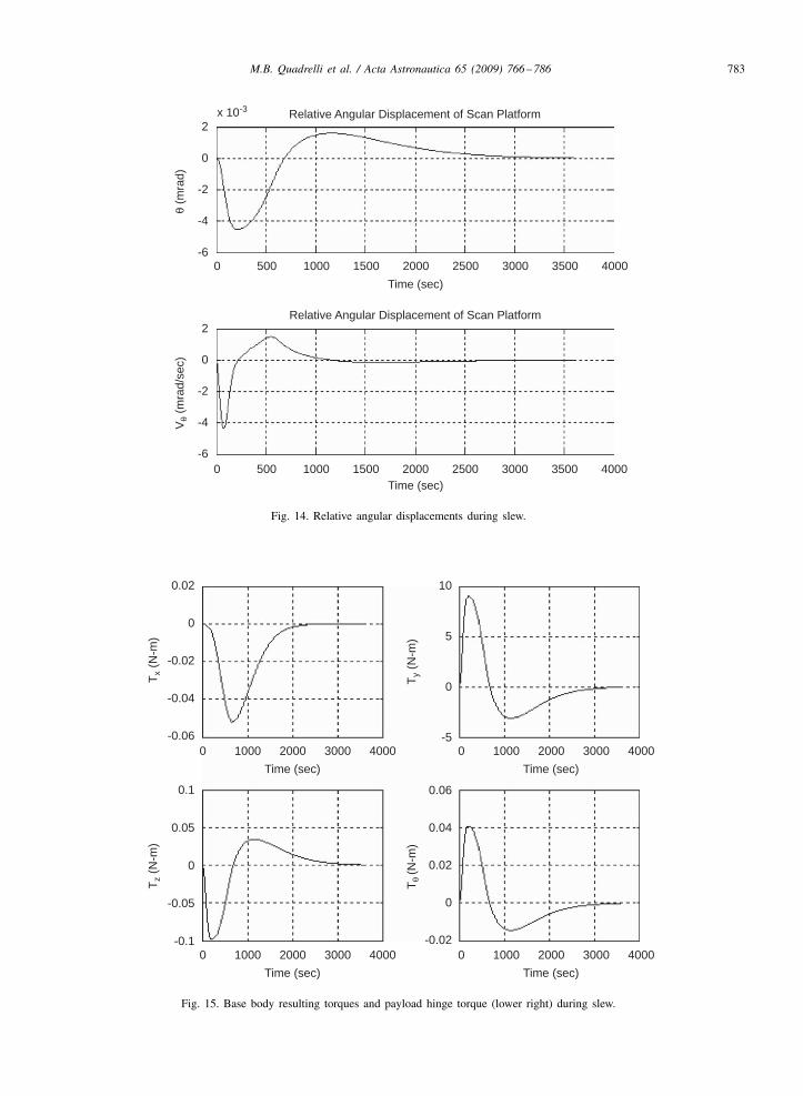
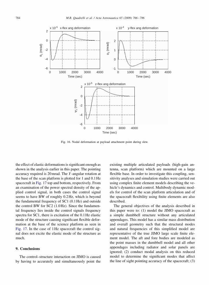
rotation was simulated for both spacecraft—one withfundamental frequency of 0.1Hz and other with 1Hz.For both simulations the same nonlinear dissipative con-trol law of Eq. (53) was used. Some selected simula-tion results for case B are shown in Fig. 14 throughFig. 16. The reference profile was chosen to be a sig-moid to allow smooth trajectory. The relative angulardisplacement for the articulated appendage is shown inFig. 14. The torque inputs are given in Fig. 15. Fig.16 shows the nodal deformation at payload attachmentpoint during slew. The effect of base body flexibility onthe relative angular orientation of the scan platform ap-pendage is given in Fig. 16 where purely rigid displace-ment and rigid plus flexible displacement is compared.As it can be seen, the flexibility effect is not significantduring this maneuver since the input torque levels arefairly small compared to the overall inertia of the space-craft. However, from pointing performance standpoint


2

0

-2

-4

-60 500 1000 1500 2000 2500 3000 3500 4000

Time (sec)

2

0

-2

-4

-60 500 1000 1500 2000 2500 3000 3500 4000

Time (sec)

Vθ

(mra

d/se

c)θ

(mra

d)

x 10-3 Relative Angular Displacement of Scan Platform

Relative Angular Displacement of Scan Platform

Fig. 14. Relative angular displacements during slew.

0.02

0

-0.02

-0.04

-0.060 1000 2000 3000 4000

Time (sec)0 1000 2000 3000 4000

Time (sec)

0 1000 2000 3000 4000Time (sec)

0 1000 2000 3000 4000Time (sec)

T x (N

-m)

T z (N

-m)

T y (N

-m)

T θ (N

-m)

0.1

0.05

0

-0.05

-0.1

0.06

0.04

0.02

0

-0.02

10

5

0

-5

Fig. 15. Base body resulting torques and payload hinge torque (lower right) during slew.


2

0

-2

-4

-60 1000 2000 3000 4000

Time (sec)

0 1000 2000 3000 4000Time (sec)

0 1000 2000 3000 4000Time (sec)

x 10-5

x 10-5

x 10-4x-flex ang deformation y-flex ang deformation

z-flex ang deformation

θ 1 (m

rad)

φ 1 (m

rad)

ψ1

(mra

d)

2

1

0

-1

2

0

-2

-4

-6

Fig. 16. Nodal deformation at payload attachment point during slew.

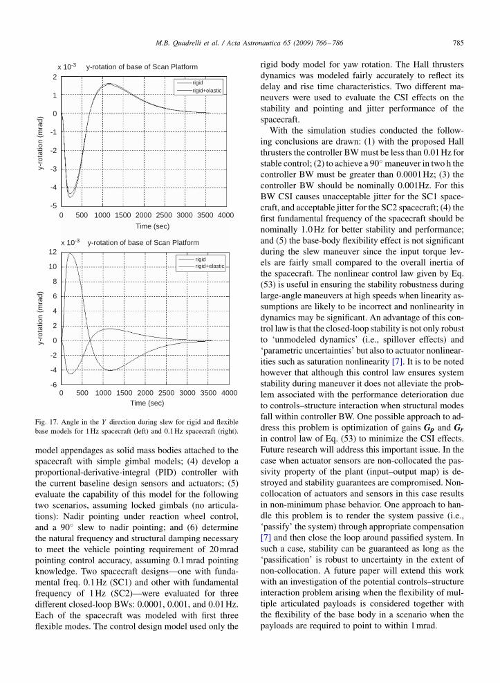
the effect of elastic deformations is significant enough asshown in the analysis earlier in this paper. The pointingaccuracy required is 20mrad. The Y -angular rotation atthe base of the scan platform is plotted for 1 and 0.1Hzspacecraft in Fig. 17 top and bottom, respectively. Froman examination of the power spectral density of the ap-plied control signal, in both cases the control signalseems to have BW of roughly 0.2Hz, which is beyondthe fundamental frequency of SC1 (0.1Hz) and outsidethe control BW for SC2 (1.0Hz). Since the fundamen-tal frequency lies inside the control signals frequencyspectra for SC1, there is excitation of the 0.1Hz elasticmode of the structure causing significant flexible defor-mation at the base of the science platform as seen inFig. 17. In the case of 1Hz spacecraft the control sig-nal does not excite the elastic mode of the structure asmuch.

9. Conclusions

The control–structure interaction on JIMO is causedby having to accurately and simultaneously point the

existing multiple articulated payloads (high-gain an-tenna, scan platform) which are mounted on a largeflexible base. In order to investigate this coupling, sen-sitivity analyses and simulation studies were carried outusing complex finite element models describing the ve-hicle’s dynamics and control. Multibody dynamic mod-els for control of the scan platform articulation and ofthe spacecraft flexibility using finite elements are alsodescribed.The general objectives of the analysis described in

this paper were to: (1) model the JIMO spacecraft asa simple dumbbell structure without any articulatedappendages. This model has a similar mass distributionand overall geometry such that the structural modesand natural frequencies of this simplified model arerepresentative of the true JIMO large scale finite ele-ment model. The aft and fore bodies are modeled asthe point masses in the dumbbell model and all otherappendages including radiator and solar panels areignored; (2) conduct modal analysis on this reducedmodel to determine the significant modes that affectthe line of sight pointing accuracy of the spacecraft; (3)


2

1

0

-1

-2

-3

-4

-50 500 1000 1500 2000 2500 3000 3500 4000

Time (sec)

0 500 1000 1500 2000 2500 3000 3500 4000Time (sec)

y-rotation of base of Scan Platformx 10-3

y-rotation of base of Scan Platformx 10-3

y-ro

tatio

n (m

rad)

y-ro

tatio

n (m

rad)

12

10

8

6

4

2

0

-2

-4

-6

rigidrigid+elastic

rigidrigid+elastic

Fig. 17. Angle in the Y direction during slew for rigid and flexiblebase models for 1Hz spacecraft (left) and 0.1Hz spacecraft (right).

model appendages as solid mass bodies attached to thespacecraft with simple gimbal models; (4) develop aproportional-derivative-integral (PID) controller withthe current baseline design sensors and actuators; (5)evaluate the capability of this model for the followingtwo scenarios, assuming locked gimbals (no articula-tions): Nadir pointing under reaction wheel control,and a 90◦ slew to nadir pointing; and (6) determinethe natural frequency and structural damping necessaryto meet the vehicle pointing requirement of 20mradpointing control accuracy, assuming 0.1mrad pointingknowledge. Two spacecraft designs—one with funda-mental freq. 0.1Hz (SC1) and other with fundamentalfrequency of 1Hz (SC2)—were evaluated for threedifferent closed-loop BWs: 0.0001, 0.001, and 0.01Hz.Each of the spacecraft was modeled with first threeflexible modes. The control design model used only the

rigid body model for yaw rotation. The Hall thrustersdynamics was modeled fairly accurately to reflect itsdelay and rise time characteristics. Two different ma-neuvers were used to evaluate the CSI effects on thestability and pointing and jitter performance of thespacecraft.With the simulation studies conducted the follow-

ing conclusions are drawn: (1) with the proposed Hallthrusters the controller BWmust be less than 0.01Hz forstable control; (2) to achieve a 90◦ maneuver in two h thecontroller BW must be greater than 0.0001Hz; (3) thecontroller BW should be nominally 0.001Hz. For thisBW CSI causes unacceptable jitter for the SC1 space-craft, and acceptable jitter for the SC2 spacecraft; (4) thefirst fundamental frequency of the spacecraft should benominally 1.0Hz for better stability and performance;and (5) the base-body flexibility effect is not significantduring the slew maneuver since the input torque lev-els are fairly small compared to the overall inertia ofthe spacecraft. The nonlinear control law given by Eq.(53) is useful in ensuring the stability robustness duringlarge-angle maneuvers at high speeds when linearity as-sumptions are likely to be incorrect and nonlinearity indynamics may be significant. An advantage of this con-trol law is that the closed-loop stability is not only robustto ‘unmodeled dynamics’ (i.e., spillover effects) and‘parametric uncertainties’ but also to actuator nonlinear-ities such as saturation nonlinearity [7]. It is to be notedhowever that although this control law ensures systemstability during maneuver it does not alleviate the prob-lem associated with the performance deterioration dueto controls–structure interaction when structural modesfall within controller BW. One possible approach to ad-dress this problem is optimization of gains Gp and Grin control law of Eq. (53) to minimize the CSI effects.Future research will address this important issue. In thecase when actuator sensors are non-collocated the pas-sivity property of the plant (input–output map) is de-stroyed and stability guarantees are compromised. Non-collocation of actuators and sensors in this case resultsin non-minimum phase behavior. One approach to han-dle this problem is to render the system passive (i.e.,‘passify’ the system) through appropriate compensation[7] and then close the loop around passified system. Insuch a case, stability can be guaranteed as long as the‘passification’ is robust to uncertainty in the extent ofnon-collocation. A future paper will extend this workwith an investigation of the potential controls–structureinteraction problem arising when the flexibility of mul-tiple articulated payloads is considered together withthe flexibility of the base body in a scenario when thepayloads are required to point to within 1mrad.


Acknowledgments

This research was carried out at the Jet PropulsionLaboratory, California Institute of Technology, under acontract with the National Aeronautics and Space Ad-ministration. The authors are grateful to Tooraj Kia,Fred Hadaegh, and Duncan MacPherson for useful dis-cussions.

References

[1] B.M. Quadrelli, E. Mettler, J.K. Langmaier, Dynamics andcontrol of a conceptual Jovian moon tour spacecraft, in: Presentedat the AAS Astrodynamics Specialist Conference, Providence,RI, August 2004.

[2] T.R. Kane, P.W. Likins, D.A. Levinson, Spacecraft Dynamics,McGraw-Hill, New York, 1984.

[3] P.C. Hughes, Spacecraft Attitude Dynamics, Prentice-Hall,Englewood Cliffs, NJ, 1986 (Chapter 9).

[4] J.L. Junkins, Y. Kim, Introduction to Dynamics and Control ofFlexible Structures, AIAA Education Series, 1993 (Chapter 4).

[5] B.M. Quadrelli, A.H. Von Flotow, Pointing dynamics of gimbaledpayloads on flexible spacecraft, Journal of Guidance, Control,and Dynamics 17 (6) (1994) 1387–1389.

[6] J.V. Coyner, J.M. Hedgepeth, H.D. Riead, Long-Boom Concepts,NASA CR-146169, September 1976.

[7] A.G. Kelkar, S.M. Joshi, Control of nonlinear multibody flexiblespace structures, Lecture Notes in Control and InformationSciences, vol. 221, Springer, Berlin, August 1996.

[8] A.G. Kelkar, S.M. Joshi, Robust control of non-passive systemsvia passification. in: Proceedings of the American ControlConference, vol. 5, Albuquerque, NM, June 4–6, 1997, pp.2657–2661.

controls structure interaction on the jupiter icy moons orbiter

Documents