the plasma environments of saturn's moons enceladus and
TRANSCRIPT
The Plasma Environments of Saturn’sMoons Enceladus and Rhea: Modeling
of Cassini Magnetic Field Data
Von der Fakultät für Elektrotechnik, Informationstechnik, Physikder Technischen Universität Carolo-Wilhelmina
zu Braunschweigzur Erlangung des Grades eines
Doktors der Naturwissenschaften(Dr.rer.nat.)genehmigteDissertation
von Hendrik Alexander Kriegelaus Braunschweig
Bibliografische Information der Deutschen Nationalbibliothek
Die Deutsche Nationalbibliothek verzeichnet diese Publikation in derDeutschen Nationalbibliografie; detaillierte bibliografische Datensind im Internet über http://dnb.d-nb.de abrufbar.
1. Referentin oder Referent: Prof. Dr. U. Motschmann2. Referentin oder Referent: Prof. Dr. J. Saureingereicht am: 17. Dezember 2013mündliche Prüfung (Disputation) am: 6. März 2014
ISBN 978-3-944072-02-9
uni-edition GmbH 2014http://www.uni-edition.dec© Hendrik Alexander Kriegel
This work is distributed under aCreative Commons Attribution 3.0 License
Printed in Germany
Vorveröffentlichungen der DissertationTeilergebnisse aus dieser Arbeit wurden mit Genehmigung der Fakultät für Elektrotech-nik, Informationstechnik, Physik, vertreten durch den Mentor der Arbeit, in folgendenBeiträgen vorab veröffentlicht:
Publikationen
• Simon, S., J. Saur, H. Kriegel, F. M. Neubauer, U. Motschmann, and M. K. Dougherty(2011a), Influence of negatively charged plume grains and hemisphere couplingcurrents on the structure of Enceladus’ Alfvén wings: Analytical modeling of Cassinimagnetometer observations, Journal of Geophysical Research (Space Physics), 116,A04221, doi: 10.1029/2010JA016338The author’s contribution: H.K. proposed the idea that the dust is responsible forthe puzzling magnetic field structures and contributed to the interpretation of theresults. The proof of the dust hypothesis and the analytical interaction model pre-sented in this paper were developed by S.S. and J.S.
• Kriegel, H., S. Simon, U. Motschmann, J. Saur, F. M. Neubauer, A. M. Persoon,M. K. Dougherty, and D. A. Gurnett (2011), Influence of negatively charged plumegrains on the structure of Enceladus’ Alfvén wings: Hybrid simulations versusCassini Magnetometer data, Journal of Geophysical Research (Space Physics), 116,A10223, doi: 10.1029/2011JA016842The author’s contribution: H.K. performed and analyzed the simulations, createdthe figures and wrote the manuscript of the article with the help of the co-authors.
• Simon, S. and Kriegel, H., Saur, J., Wennmacher, A., Neubauer, F. M., Roussos,E., Motschmann, U. and Dougherty, M. K. (2012), Analysis of Cassini magneticfield observations over the poles of Rhea, Journal of Geophysical Research (SpacePhysics), 117, A07211, doi: 10.1029/2012JA017747The author’s contribution: S.S. and H.K. contributed equally to this work: H.K.proposed the idea that a current in the wake generates the field perturbations andperformed the simulations. Further, H.K. created the figures of the simulation re-sults and helped in article writing.
• Kriegel, H., S. Simon, P. Meier, U. Motschmann, J. Saur, A. Wennmacher, D. F.Strobel, and M. K. Dougherty (2014), Ion densities and magnetic signatures of dustpick-up at Enceladus, Journal of Geophysical Research: Space Physics, pp. n/a–n/a, doi: 10.1002/2013JA019440The author’s contribution: H.K. performed and analyzed the simulations, createdthe figures and wrote the manuscript of the article with the help of the co-authors.
i
Tagungsbeiträge
• Kriegel, H., S. Simon, J. Müller, U. Motschmann, J. Saur,K. Glassmeier, and M. K.Dougherty, Hybrid Simulations of the Enceladus Plasma Interaction and Compari-son with Cassini MAG Data, Magnetospheres of the Outer Planets 2009, Köln, 27.- 31. Juli 2009, (Vortrag)
• Kriegel, H., S. Simon, U. M. Motschmann, J. S. Saur, J. Mueller, C. Koenders,K. Glassmeier, and M. K. Dougherty, Impact of ion-neutral chemistry in the Ence-ladus plume on the global plasma interaction: a hybrid simulation approach, AGUFall Meeting 2009, San Francisco, 14.–18. Dezember 2009, p. C1141, (Poster)
• Kriegel, H., S. Simon, U. Motschmann, J. Saur, J. Mueller, F. M. Neubauer, D. F.Strobel, K.-H. Glassmeier, and M. K. Dougherty , Enceladus’ variable magneto-spheric interaction: a hybrid simulation study, EGU General Assembly 2010, Wien,2. – 7. Mai 2010, p. 2860, (Poster)
• Kriegel, H., Hybrid simulations of moon-magnetosphere interactions at Saturn,AGU Fall Meeting 2010, San Francisco, 13. –17. Dezember 2010, p. D5, (einge-ladener Vortrag, ausgezeichnet mit dem ”Outstanding Student Paper Award”)
• Kriegel, H., Simon, S., Müller, J., Motschmann, U., Saur, J., Neubauer, F. M.Hybrid-Simulationen von Mond-Magnetosphären-Wechselwirkungen bei Saturn,Jahrestagung der DGG gemeinsam mit der Arbeitsgemeinschaft ExtraterrestrischeForschung und dem Fachverband Extraterrestrische Physik der DPG, Köln, 21. –24. Februar 2011, (Vortrag)
• Kriegel, H., S. Simon, U. Motschmann, J. Saur, F. M. Neubauer, A. M. Persoon,M. K. Dougherty, and D. A. Gurnett, Influence of negatively charged plume grainson the structure of Enceladus’ Alfven wings: hybrid simulations versus CassiniMAG data, Magnetospheres of the Outer Planets 2011, Boston, 11. – 15. Juli2011, (Vortrag)
• Kriegel, H. and Simon, S. and Motschmann, U. M. and Saur, J. and Neubauer,F. M. and Schmidt, J. and Teolis, B. D. and Dougherty, M. K., Hybrid simulationsof Enceladus’ plasma interaction: a multi-instrument survey, AGU Fall Meeting2011, San Francisco, 5. – 9. Dezember 2011, B2018, (Vortrag)
• Kriegel, H. and Simon, S. and Motschmann, U. and Saur, J. and Neubauer, F. M.,Hybrid simulations of dust-plasma interactions at Enceladus and comparison withCassini data, European Planetary Science Congress 2012, Madrid, 23. –28. Septem-ber 2012 , 111, Link, (Vortrag)
• Kriegel, H., The impact of Enceladus’ dust plume on the magnetic field and plasma,AGU Fall Meeting 2012, San Francisco, 3.–7. Dezember, (eingeladener Vortrag)
• Kriegel, H., Simulations of plasma-dust-neutral interactions at Enceladus, Mag-netospheres of the Outer Planets 2013, Athen, 8.–12. Juli 2013, (eingeladenerVortrag)
ii
Contents
Abstract vii
Zusammenfassung ix
1 Introduction 1
2 The Magnetospheric Environment of Enceladus and Rhea 52.1 Saturn’s Icy Moons Enceladus and Rhea . . . . . . . . . . . . . . . . . . 52.2 Plasma in Saturn’s Inner and Middle Magnetosphere . . . . . . . . . . . 102.3 Coordinate System and Flybys . . . . . . . . . . . . . . . . . . . . . . . 15
2.3.1 Enceladus Flybys . . . . . . . . . . . . . . . . . . . . . . . . . . 162.3.2 Rhea Flybys . . . . . . . . . . . . . . . . . . . . . . . . . . . . 23
2.4 Upstream Plasma Conditions at Enceladus and Rhea . . . . . . . . . . . 24
3 Basics of Enceladus’ and Rhea’s Plasma Interaction 293.1 Interaction of an Inert Moon . . . . . . . . . . . . . . . . . . . . . . . . 293.2 The Alfvén Wing . . . . . . . . . . . . . . . . . . . . . . . . . . . . . . 32
3.2.1 General Properties of the Alfvén Wing . . . . . . . . . . . . . . . 333.2.2 Mathematical Derivation . . . . . . . . . . . . . . . . . . . . . . 363.2.3 Pedersen and Hall Currents . . . . . . . . . . . . . . . . . . . . . 403.2.4 Potential Equation . . . . . . . . . . . . . . . . . . . . . . . . . 423.2.5 Solution of the Potential Equation . . . . . . . . . . . . . . . . . 44
3.3 The Alfvén Wing of Enceladus (Hemisphere Coupling) . . . . . . . . . . 493.4 Enceladus’ Plasma Interaction: Measurements and Further Studies . . . . 513.5 Summary of Enceladus’ Plasma Interaction and Open Questions . . . . . 56
4 Hybrid Simulation Code A.I.K.E.F. 594.1 Hybrid Approach: Basic Assumptions and Equations . . . . . . . . . . . 594.2 Numerical Implementation . . . . . . . . . . . . . . . . . . . . . . . . . 624.3 Collisions, Reactions and Ionization . . . . . . . . . . . . . . . . . . . . 64
4.3.1 Reaction Probability and Implementation . . . . . . . . . . . . . 664.3.2 Comparison of Statistical Collisions and Fluid Drag Force . . . . 674.3.3 Photoionization and Electron Impact Ionization . . . . . . . . . . 69
4.4 Numerical Damping (Smoothing) . . . . . . . . . . . . . . . . . . . . . 714.5 Boundary Conditions . . . . . . . . . . . . . . . . . . . . . . . . . . . . 76
4.5.1 Inner boundary . . . . . . . . . . . . . . . . . . . . . . . . . . . 764.5.2 Outer boundaries . . . . . . . . . . . . . . . . . . . . . . . . . . 79
iii
Contents
4.6 Further Simulation Codes for Enceladus and Rhea . . . . . . . . . . . . . 81
5 Influence of Dust on Enceladus’ Alfvén Wings 835.1 Magnetic Field Observations at Enceladus . . . . . . . . . . . . . . . . . 835.2 Anti-Hall Effect: Analytical Derivation . . . . . . . . . . . . . . . . . . . 865.3 Anti-Hall Effect: Simulations . . . . . . . . . . . . . . . . . . . . . . . . 905.4 Modeling Enceladus . . . . . . . . . . . . . . . . . . . . . . . . . . . . 94
5.4.1 Simulation Parameters and Geometry . . . . . . . . . . . . . . . 945.4.2 Modeling the Plume . . . . . . . . . . . . . . . . . . . . . . . . 965.4.3 Dusty Plasma Parameters . . . . . . . . . . . . . . . . . . . . . . 98
5.5 Results for Selected Enceladus Flybys . . . . . . . . . . . . . . . . . . . 985.5.1 Density and Velocity . . . . . . . . . . . . . . . . . . . . . . . . 995.5.2 Magnetic Field: E5 and E6 . . . . . . . . . . . . . . . . . . . . . 1015.5.3 Magnetic Field: E7 and E9 . . . . . . . . . . . . . . . . . . . . . 1045.5.4 Magnetic Field: E8 and E11 . . . . . . . . . . . . . . . . . . . . 107
5.6 Variability of the Plume . . . . . . . . . . . . . . . . . . . . . . . . . . . 1095.7 Anti-Hall Condition at Enceladus . . . . . . . . . . . . . . . . . . . . . . 110
6 Ion Densities and Magnetic Signatures of Dust Pick-up at Enceladus 1136.1 Simulation Model . . . . . . . . . . . . . . . . . . . . . . . . . . . . . . 114
6.1.1 Simulation Parameters . . . . . . . . . . . . . . . . . . . . . . . 1156.1.2 Ion-Neutral Chemistry . . . . . . . . . . . . . . . . . . . . . . . 1176.1.3 Photo- and Electron Impact Ionization . . . . . . . . . . . . . . . 118
6.2 Modeling of Neutral Plume . . . . . . . . . . . . . . . . . . . . . . . . 1206.3 Modeling of the Dust Plume . . . . . . . . . . . . . . . . . . . . . . . . 1286.4 Results I: Plasma Densities . . . . . . . . . . . . . . . . . . . . . . . . . 131
6.4.1 Ion Composition . . . . . . . . . . . . . . . . . . . . . . . . . . 1316.4.2 Ion Densities . . . . . . . . . . . . . . . . . . . . . . . . . . . . 1336.4.3 Dust Charge Density . . . . . . . . . . . . . . . . . . . . . . . . 137
6.5 Results II: Magnetic Field Signatures . . . . . . . . . . . . . . . . . . . . 1406.5.1 Magnetic Field Signatures for Different Neutral Plumes (E7) . . . 1416.5.2 Influence of Dust Current (E17) . . . . . . . . . . . . . . . . . . 1426.5.3 Pick-up and Length of Dust Plume (E14 and E19) . . . . . . . . . 1456.5.4 Distant Nanograin Pick-Up (E15) . . . . . . . . . . . . . . . . . 1506.5.5 The ”Missing” Magnetic Field Decrease (E14 and E19) . . . . . . 1516.5.6 Plume Variability . . . . . . . . . . . . . . . . . . . . . . . . . . 153
7 Analysis of Cassini magnetic field observations over the poles of Rhea 1557.1 Magnetic visibility of Rhea’s exosphere . . . . . . . . . . . . . . . . . . 1567.2 Rhea flybys R2 and R3 . . . . . . . . . . . . . . . . . . . . . . . . . . . 158
7.2.1 Flyby R3: MAG data . . . . . . . . . . . . . . . . . . . . . . . . 1587.2.2 Flyby R3: Hybrid simulations . . . . . . . . . . . . . . . . . . . 164
7.2.2.1 Model description and input parameters . . . . . . . . 1657.2.2.2 Discussion of simulation results . . . . . . . . . . . . . 165
7.2.3 Flyby R2: MAG observations and hybrid simulations . . . . . . . 174
iv
Contents
8 Summary and Outlook 1798.1 Enceladus . . . . . . . . . . . . . . . . . . . . . . . . . . . . . . . . . . 1798.2 Rhea . . . . . . . . . . . . . . . . . . . . . . . . . . . . . . . . . . . . . 1838.3 Outlook . . . . . . . . . . . . . . . . . . . . . . . . . . . . . . . . . . . 185
A Reaction and Ionization Rates 189
B Magnetic Field Signatures from Further Enceladus Flybys 193B.1 The Encounters E1, E10 and E16 . . . . . . . . . . . . . . . . . . . . . . 193B.2 Magnetic Field Structures Resulting from the Improved Model Along E5
and E6 . . . . . . . . . . . . . . . . . . . . . . . . . . . . . . . . . . . . 194B.3 The E2 Flyby in the Context of Charged Dust . . . . . . . . . . . . . . . 197B.4 The North Polar Flybys E12 and E13 . . . . . . . . . . . . . . . . . . . . 198
C Simulations of the Dione D3 Flyby 201
Bibliography 205
Acknowledgements 221
v

Abstract
One of the most fascinating discoveries of the Cassini mission was the extended plume ofwater vapor and ice grains below Saturn’s small moon Enceladus. The plume originatesfrom geyser-like jets that are probably fed by a subsurface ocean of liquid water. Thesejets are located within surface fractures at the moon’s south polar regions, the so-called”tiger stripes”. After leaving their sources, the neutrals are ionized by means of photoion-ization and charge exchange with Saturn’s magnetospheric plasma, thereby generatingcurrents which perturb the plasma flow as well as Saturn’s dipolar magnetic field. Moreprecisely, these currents are closed by a system of field-aligned currents, the Alfvén wing.In this thesis, analytical models as well as numerical simulations by means of the hybridcode A.I.K.E.F. (Adaptive Ion-Kinetic Electron-Fluid) are applied to study the interactionof the magnetospheric plasma with the Enceladean plume. In particular, the magneticfield perturbations generated by the interaction are analyzed and the simulation resultsare compared with Cassini Magnetometer (MAG) data obtained during the 20 Enceladusflybys (labeled E0 – E19), which took place between 2005 and 2013.In a first study, it is shown that electron absorption by dust leads to a negative sign ofthe Hall conductivity and an associated reversal of the Hall current, which is referred toas the ”Anti-Hall effect”. The resulting twist of the magnetic field has been observedduring all targeted Enceladus flybys so far. When including the dust, the simulations arein quantitative agreement with Cassini MAG data.In a second study, the plasma simulations are combined with Monte-Carlo simulationsof the 3D profiles of the water and dust plumes. Thereby, the improved model for thefirst time includes the effect of the distorted electromagnetic fields on the motion of thecharged dust grains. Furthermore, the obtained neutral plume profiles are in excellentagreement with Cassini data, allowing to quantitatively analyze the ion densities withinthe plume. It is also demonstrated that the magnetic field signatures indicate the pick-upof negatively charged nanograins.In addition, Cassini magnetic field observations from the only two polar flybys of Saturn’slargest icy satellite Rhea are analyzed (R2 on 02 March 2010 and R3 on 11 January2011). In-situ observations of exospheric neutral gas suggest Rhea to be embedded ina tenuous gas envelope. However, the interaction of this gas with the magnetosphericplasma does not cause any measurable contributions to the magnetic field draping patterndetected above the poles of the moon. Instead, it is shown that the finite length of Rhea’swake leads to a diamagnetic current that is responsible for generating a weak Alfvénwing pattern which has been detected by the Cassini spacecraft during the R2 and R3encounters.
vii

Kurzzusammenfassung
Eine der spektakulärsten Entdeckungen der Cassini-Mission war die Beobachtung einergroßen Wolke aus Wasserdampf und nm- bis µm-großen Eispartikeln unterhalb von Sat-urns kleinem Eismond Enceladus, des sogenannten ”Plumes”. Dieser wird von geysir-artigen Jets gebildet, die sich in Schluchten in der Südpolarregion, den sogenannten”Tigerstreifen”, befinden und die vermutlich durch einen unterirdischen Ozean aus flüs-sigem Wasser gespeist werden. Nach dem Ausströmen werden die Neutralgasmoleküledurch Photoionisation und Ladungsaustausch mit Saturns magnetosphärischem Plasmaionisiert, wodurch sie Ströme erzeugen, die sowohl das Plasma als auch Saturns mag-netisches Dipolfeld beeinflussen. Genauer gesagt werden diese Ströme durch ein Systemvon feldparallelen Strömen, dem Alfvén-Flügel, geschlossen.Das Ziel dieser Arbeit ist die Untersuchung der Wechselwirkung von Saturns magne-tosphärischem Plasma mit Enceladus und seinem Plume. Hierzu werden sowohl analy-tische Modelle als auch numerische Simulationen mittels des Hybrid-Codes (AdaptiveIon-Kinetic Electron-Fluid) verwendet. Insbesondere werden die durch die Wechsel-wirkung erzeugten Magnetfeldstrukturen untersucht und die Ergebnisse mit Cassini Mag-netometer (MAG) Messungen von den 20 Enceladus-Vorbeiflügen (E0 – E19), die zwis-chen 2005 und 2013 stattfanden, verglichen.In einer ersten Studie wird gezeigt, dass die Absorption von Elektronen durch den Staubzu einem negativen Vorzeichen der Hall-Leitfähigkeit und einer damit verbundenen Um-kehr des Hall-Stroms führt. Dieser Effekt wurde von uns ”Anti-Hall Effekt” getauft.Die daraus resultierende Verdrehung der Magnetfeldlinien innerhalb des Alfvén-Flügelswurde während aller Enceladus-Vorbeiflüge gemessen. Durch die Einbeziehung des Stau-bes stimmen die Simulationsergebnisse quantitativ mit Cassini MAG-Daten überein.In einer zweiten Studie werden die Plasmasimulationen mit Monte-Carlo Simulationender 3D-Struktur des Neutralgas- und Staubplumes kombiniert. Dadurch berücksichtigtdas Modell erstmalig den Einfluss der gestörten elektromagnetischen Felder auf die Be-wegung der geladenen Staubteilchen. Darüber hinaus ist die Übereinstimmung der ausden Simulationen resultierenden Struktur des Neutralgasplumes mit Cassini-Messungensehr gut, was eine quantitative Analyse der Ionendichten im Plume ermöglicht. Es wirdzudem gezeigt, dass die gemessenen Magnetfeldsignaturen auf den Pick-up von negativgeladenen Nanoteilchen hinweisen.Des Weiteren werden Magnetfeldmessungen von Cassini von den zwei einzigen polarenVorbeiflügen an Saturns zweitgrößtem Mond Rhea (R2 am 2. März 2010 und R3 am 11.Januar 2011) analysiert. In-situ-Beobachtungen von exosphärischem Neutralgas zeigen,dass Rhea von einer dünnen Neutralgashülle umgeben ist. Die Wechselwirkung des Plas-
ix

Kurzzusammenfassung
mas mit dem Neutralgas verursacht jedoch keine nennenswerten Magnetfeldstörungenüber Rheas Polen. Stattdessen wird gezeigt, dass die endliche Länge von Rheas Plasma-Wake zu einem diamagnetischen Strom führt. Dieser Strom erzeugt wiederum einenschwachen Alfvén-Flügel, dessen Magnetfeldsignatur von Cassini während der R2- undR3-Vorbeiflüge detektiert wurde.
x
1 Introduction
Out of the 62 known Saturnian moons1, the seven major ones have already been discov-ered in the 17th and 18th century. While Titan has first been observed by ChristiaanHuygens in 1655, Saturn’s second largest moon, Rhea, was discovered on 23 Decem-ber 1672 by Giovanni Cassini along with Dione, Tethys and Iapetus. The inner satellitesEnceladus and Mimas were discovered about 100 years later on 28 August 1789 and 17September 1789, respectively, by Sir William Herschel [Herschel 1790]. However, it wasnot before 1847 that the current names of the moons were proposed by Herschel’s sonJohn [Herschel 1847]:
“As Saturn devoured his children, his family could not be resembled roundhim, so that the choice lay among his brothers and sisters, the Titans andTitanesses. The name (...) Titan seemed to be indicated by the superior size ofthe Huygenian, while the three female appellatives (Rhea, Dione and Tethys)class together the three intermediate Cassinian satellites. The minute interiorsatellites (Enceladus and Mimas) seemed appropriately characterized by areturn to male appellatives, chosen from a younger and inferior (though stillsuperhuman) brood.“
The first close-up images of these Titanesses and Titans as well as Saturn itself werecaptured during the flybys of the two Voyager spacecrafts in the 1980s. To further in-crease the knowledge of the giant planet and its moons and rings, the US National Aero-nautics and Space Administration (NASA), the European Space Agency (ESA) and Ital-ian space agency Agenzia Spaziale Italiana (ASI) designed the joint mission Cassini-Huygens. Launched in 1997, the spacecraft arrived at Saturn on 1 July 2004. On 14January 2005, the Huygens probe was successfully delivered to Titan. The Cassini or-biter – equipped with twelve scientific instruments – completed its initial four-year primemission of exploration in the Saturnian system in June 2008. The subsequent first ex-tended mission, called the Cassini Equinox Mission, lasted until September 2010, whilethe second extended mission ”Solstice” (named after the Saturnian summer solstice inMay 2017) will hopefully be continued until September 2017 with ongoing success.This thesis focuses on two particular members of Saturn’s family of moons, namely theicy satellites Enceladus and Rhea. In addition, a tiny part of this work is dedicated toEnceladus’ neighbor Dione. Although Enceladus was called a ’minute and inferior satel-lite’ by John Herschel, this view has changed considerably with the spectacular discoveryof the Enceladus plume – a large cloud of water vapor and ice grains emanating from the
1State: 2013
1
1 Introduction
moon’s south polar regions – by the Cassini Magnetometer [Dougherty et al. 2006]. Theplume originates from geyser-like jets which are almost certainly being fed by a subsur-face ocean of liquid water. The finding of present-day cryovolcanism promoted Enceladusto one of Cassini’s main targets with 23 closed flybys scheduled for the whole mission. Itturned out that Enceladus’ plume constitutes the major source of neutral gas and plasmawithin the Saturnian magnetosphere. By chance, the name Enceladus is already linked tothe moon’s cryovolcanic activity. In Greek mythology, the giant Enceladus was defeatedby the goddess Athena, who smashed the island of Silicy onto him. It is said that everynow and then, Enceladus shifts his side in his grave, resulting in earthquakes and erup-tions of Mount Etna2. Unlike Enceladus, Rhea is an inactive icy moon which possessesonly a very thin atmosphere produced by sputtering [Saur and Strobel 2005]. The discov-ery that Rhea possesses a tenuous ring system on its own [Jones et al. 2008] could not beconfirmed by optical observations [Tiscareno et al. 2010].Enceladus and Rhea encircle the giant planet at distances of 3.95 and 8.74 Saturn radii(RS ), respectively. Both moons are therefore located well within Saturn’s magnetospherewhich has a sunward extent of about 20 RS . Similar to Jupiter, the Saturnian magneto-sphere is (at least partially) dominated by the fast rotation of the giant planet. Therefore,the magnetospheric plasma – which is mainly produced by ionization of the extendedneutral torus generated by the Enceladean plume – corotates or at least sub-corotates withthe planet. As the plasma flow velocity is larger than the Keplarian velocity of the moons,the ions and electrons continuously impinge on the surfaces and atmospheres of the satel-lites, whereas the plume acts like a strong, but displaced, dense atmosphere. Ionization ofthe neutral molecules of the plume by charge exchange with the magnetospheric plasma,photoionization and electron impacts and the subsequent pick-up of the new-born ionslead to the generation of electric currents. These currents and the associated perturbationsof Saturn’s dipolar magnetic field, as well as the modifications of the plasma flow and itsdensity, are in the following referred to as ’plasma interaction’.The primary aim of this thesis is to improve our understanding of the physical processesinvolved in the plasma interactions of Enceladus and Rhea on the basis of data collected byCassini. Especially Cassini Magnetometer observations obtained along the trajectories ofthe various close flybys shall be analyzed and placed within a three-dimensional context.Eventually, these magnetic field signatures allow to draw conclusions on the properties ofthe obstacle that generated them, i. e. in particular the Enceladus plume and its underlyingsources. To analyze the plasma structures, both, analytical and numerical modeling isapplied. While an analytical description is most suitable to address the basic effects, aquantitative comparison with Cassini data requires a realistic model of the obstacle in athree-dimensional geometry which can only be achieved by numerical models.Depending on the features which should be addressed, different approaches for the de-scription of the plasma can be employed. The most simple one is Magnetohydrodynam-ics (MHD), treating the plasma as a single conducting fluid. The advantage of this rathercrude approximation is the simplicity of the governing equations. These allow even withanalytical models a profound discussion of the basic features of the respective interaction.When solved numerically, MHD codes are fast to run and achieve a high resolution. Forexample, the BATS’R’US code has been applied to study Enceladus’ plasma interaction
2http://www.theoi.com/Gigante/GiganteEnkelados.html
2
1 Introduction
by Jia et al. [2010b,c]. The major drawback of the MHD is, however, that neither thedensities of different plasma species nor their different velocities can be resolved. Thenext, more sophisticated step in the hierarchy of the plasma descriptions is the multi-fluid approach, meaning that each plasma species is considered as its own fluid. Formany space physics applications, a multi-fluid code is sufficient to cover most physicaleffects which are relevant on a global scale. Due to the closure of the equations, however,only a small number of moments of the distribution function is considered by the fluidapproaches. Therefore, these models cannot account for non-Maxwellian velocity distri-butions like the ring distribution of the pick-up ions near Enceladus. In contrast to thefluid models, a fully kinetic description of both, electrons and ions, would theoreticallyinclude all possible effects. But, even with massive computational resources, it is not yetpossible to simultaneously consider the vastly different masses of electrons and ions andthe corresponding time scales.Between the fluid and the full particle descriptions lies the hybrid approach, which treatsthe ions as particles and the electrons as a massless, charge-neutralizing fluid. One of thefirst three-dimensional hybrid codes with application to space physics has been developedby Bagdonat and Motschmann [2002a] (the ”Braunschweig-Code”). In this thesis, its suc-cessor A.I.K.E.F. (Adaptive Ion-Kinetic Electron-Fluid) is applied, which is parallelizedand allows to use an adaptive mesh [Müller et al. 2011]. A.I.K.E.F. and its precursor havealready been used for the successful modeling of a large variety of plasma interactions inour solar system, e. g. the solar wind interaction of the terrestrial planets Mercury, Venus,Mars as well as the magnetospheric interaction of Saturn’s largest moons Titan and Rhea(e.g, Müller et al. [2012], Martinecz et al. [2009], Bößwetter et al. [2004], Simon et al.[2007], Roussos et al. [2008a]). The code has also been used for a pilot study of Ence-ladus’ plasma interaction [Kriegel et al. 2009]. Apart from A.I.K.E.F., a variety of otherhybrid codes is currently applied by the space plasma physics community to the plasmainteractions of the Saturnian moons, see e. g. Ledvina et al. [2004], Omidi et al. [2010,2012] and Lipatov et al. [2012]. The advantage of the hybrid model is that the kineticbehavior of the ions is included, which is particularly important for Rhea, where the iongyroradius is of about the same size as the radius of Rhea. At Enceladus, however, theion gyroradii are significantly smaller than the moon’s radius. Therefore, a fluid approachseems to be suitable for the description of Enceladus plasma interaction. However, themajor result of this thesis is that the inclusion of charged dust grains is of vital importancefor the correct description of the interaction. This plasma component could be integratedin the hybrid model without noteworthy modifications, while the available fluid simula-tion codes that are applied to Enceladus’ plasma interaction by Jia et al. [2012] and Patyet al. [2011] seem to fail to include the heavy dust. Thus, the hybrid simulation codeA.I.K.E.F. can be regarded as the appropriate choice for modeling the plasma interactionsof the Titaness Rhea and the ”little Titan” Enceladus.Enceladus and its plume are embedded in a similar magnetospheric environment as the Jo-vian moon Io with its volcano-originating sulfur atmosphere. Io’s interaction has alreadybeen studied extensively in the framework of the Voyager flybys and the Galileo missionto Jupiter in the 1980s and 1990s. The main aspect of Io’s plasma interaction is the gener-ation of a system of non-linear, standing Alfvén waves, the Alfvén wing [Neubauer 1980,1998]. However, its plume makes Enceladus unique in several aspects: the south-polar
3
1 Introduction
plume introduces an asymmetry compared to all other solar system objects which possessa rather symmetrical atmosphere/ionosphere. Therefore, particle absorption and currentblockage at the surface mix up with the alfvénic interaction of the plume, resulting inafore unknown physical processes [Saur et al. 2007, Kriegel et al. 2009]. With regard tothe so far poorly understood generation of the plume jets it is also important to determinethe degree of plume variability. The magnetic field observations of the first three flybyshave already proven to be a useful tool for the analysis of the variability [Saur et al. 2008].The magnetic field perturbations will therefore be used to constrain the shape of the plumeas well as the strength of its variability on a flyby-to-flyby base. In addition, the plumeconsists to a considerable amount of charged dust. The main result of this thesis is thatthis dust population makes ”Enceladus Plume a New Kind of Plasma Laboratory”3.Like for Earth’s moon, Rhea’s plasma interaction is dominated by the absorption of parti-cles at the surface and the resulting density cavity downstream of the moon. Prior to thiswork, only two Cassini flybys of Rhea were available, which confirmed the overall pictureof the lunar-type plasma interaction [Khurana et al. 2008, Roussos et al. 2008a]. How-ever, the trajectories of these flybys were located in Rhea’s equatorial plane and therefore,a draping of the magnetic field lines around the thin atmosphere could not have been de-tected. Hence, one aim of this thesis is to investigate whether magnetic field observationsof the two more recent, polar Rhea flybys match the expected structures of a lunar-typeinteraction.This thesis is organized as follows: in chapter 2, an overview of the magnetosphericenvironment of Enceladus and Rhea will be provided. Furthermore, the trajectories ofthe 23 Enceladus and five Rhea flybys will be described. Chapter 3 presents the stateof knowledge about Enceladus’ and Rhea’s plasma interactions prior to this thesis. Thestructures arising from plasma absorption at the moons’ surfaces as well as the generalproperties of the Alfvén wing will be discussed. The hybrid code A.I.K.E.F. will bedescribed in chapter 4. In particular, it will be elaborated on how ion-neutral reactions areincluded in the model. Moreover, the impact of the boundary conditions applied in thecode will be analyzed. Our results are presented in chapters 5 – 7:
• Chapter 5 deals with the influence of charged dust on the structure of Enceladus’Alfvén wings in the context of Cassini magnetometer observations.
• In chapter 6, Monte-Carlo simulations of the Enceladus plume are combined withthe hybrid code. Therefore, the full dust-plasma coupling in both directions is in-cluded, i. e. the dust is affected by the electromagnetic fields and plasma momentsand vice versa. The improved model allows to constrain the ion densities within theplume and to analyze the magnetic signatures of dust pick-up at Enceladus.
• An analysis of Cassini magnetic field observations over the poles of Rhea is pre-sented in chapter 7.
Finally, chapter 8 summarizes the results and gives an outlook to future work. In addition,a very brief overview about Dione’s plasma environment will be provided in appendix C.
3http://www.nasa.gov/mission_pages/cassini/whycassini/cassini20120531.html
4
2 The Magnetospheric Environment ofEnceladus and Rhea
2.1 Saturn’s Icy Moons Enceladus and Rhea
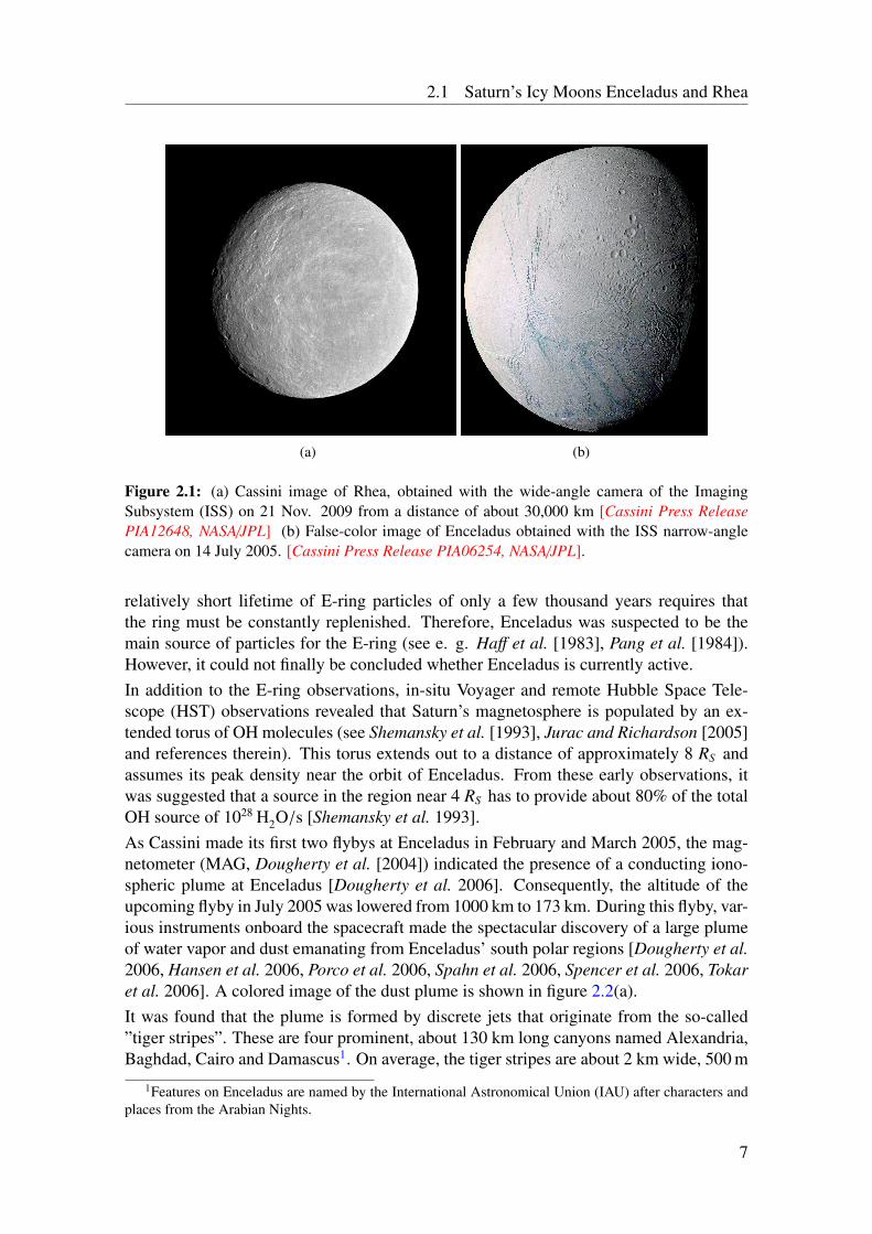
The small moon Enceladus (radius RE = 252.1 km) and Saturn’s second-largest moonRhea (RRH = 763.5 km) encircle the giant planet on orbits with eccentricities of lessthan ε = 0.005 (see table 2.1 for a list of the moons’ main physical and dynamicalproperties). With a semi-major axis of 238,040 km or 3.95 Saturn radii (equatorial ra-dius RS = 60, 268 km), Enceladus is the fourteenth satellite when ordered by distancefrom Saturn. One bound rotation is carried out in about 1.37 days. Going further awayfrom Saturn, Enceladus’ nearest neighbors are Dione – which is connected to Enceladusthrough a 2:1 orbital resonance –, Tethys and Rhea. As the outermost of these four satel-lites, Rhea’s orbit is located at 527,070 km or 8.74 RS , leading to a rotation period ofabout 108h 25min. Since their surfaces are mostly covered with water ice, the four moons(Enceladus, Dione, Tethys, Rhea) and Enceladus’ inner neighbor Mimas are also namedSaturn’s major icy moons. Their icy surfaces are also the reason why the moons haverelatively high albedos and low temperatures – Enceladus has a visual geometric albedoof 1.38 [Verbiscer et al. 2007], which makes the moon even the most reflecting celestialbody in the solar system. The corresponding surface temperature is only 76 K at the sub-solar point [Howett et al. 2010]. When compared with Enceladus, Rhea’s surface is ratherdark with an albedo of 0.95. The surface temperature ranges between 53 K in the shadowand 99 K in the sunlight [Howett et al. 2010].From the time of their discovery until the Voyager 1 spacecraft passed through the Sat-urnian system in November 1980, little more was known about the two satellites thantheir physical and dynamical characteristics (although the latest values from Cassini mea-surements are provided in table 2.1, most of these numbers have undergone only slightchanges since the pre-Voyager era). This changed when Voyager 1 and 2 sent the firsthigh-resolution images to Earth.The images of Voyager 1 showed that Rhea’s surface is more heavily cratered than thoseof the other outer moons indicating less resurfacing than at the other icy moons (cf. theimage of Rhea obtained by Cassini in figure 2.1(a)). In agreement with this finding, Rheaseemed to be a relatively unspectacular and inactive satellite. Therefore it was a big sur-prise, when Cassini observations of absorption signatures of energetic electrons seemedto imply that Rhea possesses a ring system on its own [Jones et al. 2008]. However, thepresence of this ring system has been ruled out by optical observations [Tiscareno et al.
5
2 The Magnetospheric Environment of Enceladus and Rhea
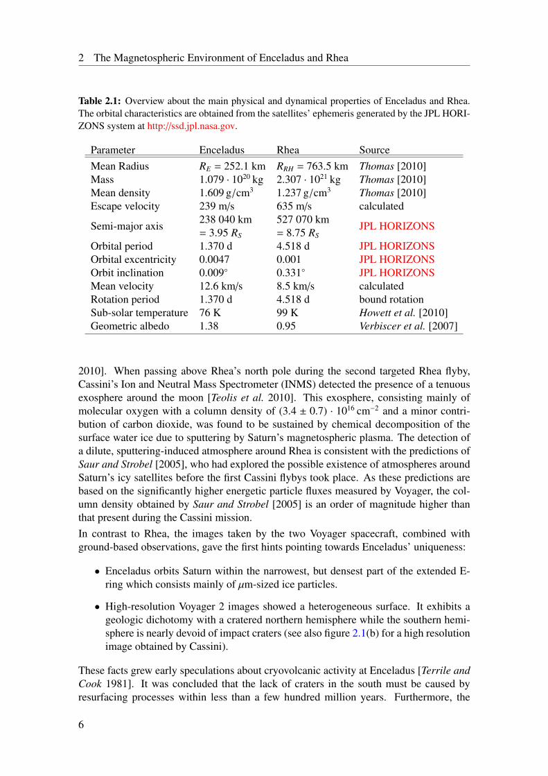
Table 2.1: Overview about the main physical and dynamical properties of Enceladus and Rhea.The orbital characteristics are obtained from the satellites’ ephemeris generated by the JPL HORI-ZONS system at http://ssd.jpl.nasa.gov.
Parameter Enceladus Rhea SourceMean Radius RE = 252.1 km RRH = 763.5 km Thomas [2010]Mass 1.079 · 1020 kg 2.307 · 1021 kg Thomas [2010]Mean density 1.609 g/cm3 1.237 g/cm3 Thomas [2010]Escape velocity 239 m/s 635 m/s calculated
Semi-major axis238 040 km 527 070 km
JPL HORIZONS= 3.95 RS = 8.75 RS
Orbital period 1.370 d 4.518 d JPL HORIZONSOrbital excentricity 0.0047 0.001 JPL HORIZONSOrbit inclination 0.009 0.331 JPL HORIZONSMean velocity 12.6 km/s 8.5 km/s calculatedRotation period 1.370 d 4.518 d bound rotationSub-solar temperature 76 K 99 K Howett et al. [2010]Geometric albedo 1.38 0.95 Verbiscer et al. [2007]
2010]. When passing above Rhea’s north pole during the second targeted Rhea flyby,Cassini’s Ion and Neutral Mass Spectrometer (INMS) detected the presence of a tenuousexosphere around the moon [Teolis et al. 2010]. This exosphere, consisting mainly ofmolecular oxygen with a column density of (3.4 ± 0.7) · 1016 cm−2 and a minor contri-bution of carbon dioxide, was found to be sustained by chemical decomposition of thesurface water ice due to sputtering by Saturn’s magnetospheric plasma. The detection ofa dilute, sputtering-induced atmosphere around Rhea is consistent with the predictions ofSaur and Strobel [2005], who had explored the possible existence of atmospheres aroundSaturn’s icy satellites before the first Cassini flybys took place. As these predictions arebased on the significantly higher energetic particle fluxes measured by Voyager, the col-umn density obtained by Saur and Strobel [2005] is an order of magnitude higher thanthat present during the Cassini mission.In contrast to Rhea, the images taken by the two Voyager spacecraft, combined withground-based observations, gave the first hints pointing towards Enceladus’ uniqueness:
• Enceladus orbits Saturn within the narrowest, but densest part of the extended E-ring which consists mainly of µm-sized ice particles.
• High-resolution Voyager 2 images showed a heterogeneous surface. It exhibits ageologic dichotomy with a cratered northern hemisphere while the southern hemi-sphere is nearly devoid of impact craters (see also figure 2.1(b) for a high resolutionimage obtained by Cassini).
These facts grew early speculations about cryovolcanic activity at Enceladus [Terrile andCook 1981]. It was concluded that the lack of craters in the south must be caused byresurfacing processes within less than a few hundred million years. Furthermore, the
6
2.1 Saturn’s Icy Moons Enceladus and Rhea
(a) (b)
Figure 2.1: (a) Cassini image of Rhea, obtained with the wide-angle camera of the ImagingSubsystem (ISS) on 21 Nov. 2009 from a distance of about 30,000 km [Cassini Press ReleasePIA12648, NASA/JPL] (b) False-color image of Enceladus obtained with the ISS narrow-anglecamera on 14 July 2005. [Cassini Press Release PIA06254, NASA/JPL].
relatively short lifetime of E-ring particles of only a few thousand years requires thatthe ring must be constantly replenished. Therefore, Enceladus was suspected to be themain source of particles for the E-ring (see e. g. Haff et al. [1983], Pang et al. [1984]).However, it could not finally be concluded whether Enceladus is currently active.In addition to the E-ring observations, in-situ Voyager and remote Hubble Space Tele-scope (HST) observations revealed that Saturn’s magnetosphere is populated by an ex-tended torus of OH molecules (see Shemansky et al. [1993], Jurac and Richardson [2005]and references therein). This torus extends out to a distance of approximately 8 RS andassumes its peak density near the orbit of Enceladus. From these early observations, itwas suggested that a source in the region near 4 RS has to provide about 80% of the totalOH source of 1028 H2O/s [Shemansky et al. 1993].As Cassini made its first two flybys at Enceladus in February and March 2005, the mag-netometer (MAG, Dougherty et al. [2004]) indicated the presence of a conducting iono-spheric plume at Enceladus [Dougherty et al. 2006]. Consequently, the altitude of theupcoming flyby in July 2005 was lowered from 1000 km to 173 km. During this flyby, var-ious instruments onboard the spacecraft made the spectacular discovery of a large plumeof water vapor and dust emanating from Enceladus’ south polar regions [Dougherty et al.2006, Hansen et al. 2006, Porco et al. 2006, Spahn et al. 2006, Spencer et al. 2006, Tokaret al. 2006]. A colored image of the dust plume is shown in figure 2.2(a).It was found that the plume is formed by discrete jets that originate from the so-called”tiger stripes”. These are four prominent, about 130 km long canyons named Alexandria,Baghdad, Cairo and Damascus1. On average, the tiger stripes are about 2 km wide, 500 m
1Features on Enceladus are named by the International Astronomical Union (IAU) after characters andplaces from the Arabian Nights.
7
2 The Magnetospheric Environment of Enceladus and Rhea
(a) (b)
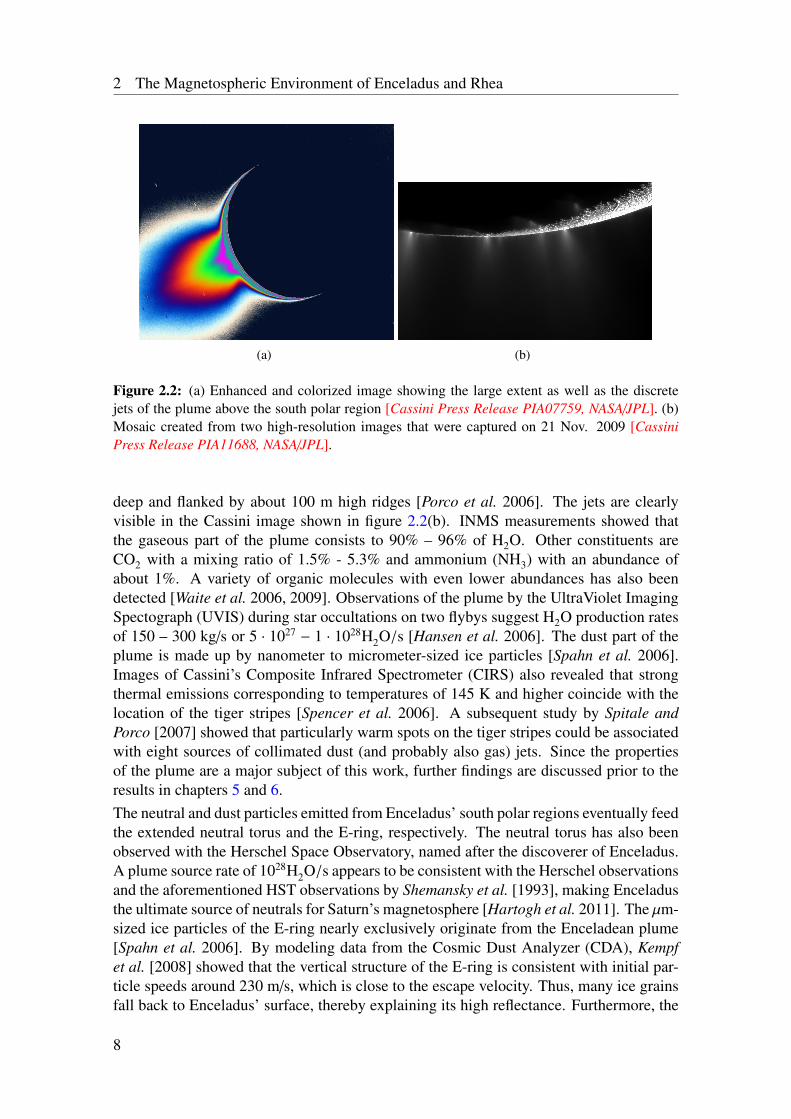
Figure 2.2: (a) Enhanced and colorized image showing the large extent as well as the discretejets of the plume above the south polar region [Cassini Press Release PIA07759, NASA/JPL]. (b)Mosaic created from two high-resolution images that were captured on 21 Nov. 2009 [CassiniPress Release PIA11688, NASA/JPL].
deep and flanked by about 100 m high ridges [Porco et al. 2006]. The jets are clearlyvisible in the Cassini image shown in figure 2.2(b). INMS measurements showed thatthe gaseous part of the plume consists to 90% – 96% of H2O. Other constituents areCO2 with a mixing ratio of 1.5% - 5.3% and ammonium (NH3) with an abundance ofabout 1%. A variety of organic molecules with even lower abundances has also beendetected [Waite et al. 2006, 2009]. Observations of the plume by the UltraViolet ImagingSpectograph (UVIS) during star occultations on two flybys suggest H2O production ratesof 150 – 300 kg/s or 5 · 1027 − 1 · 1028H2O/s [Hansen et al. 2006]. The dust part of theplume is made up by nanometer to micrometer-sized ice particles [Spahn et al. 2006].Images of Cassini’s Composite Infrared Spectrometer (CIRS) also revealed that strongthermal emissions corresponding to temperatures of 145 K and higher coincide with thelocation of the tiger stripes [Spencer et al. 2006]. A subsequent study by Spitale andPorco [2007] showed that particularly warm spots on the tiger stripes could be associatedwith eight sources of collimated dust (and probably also gas) jets. Since the propertiesof the plume are a major subject of this work, further findings are discussed prior to theresults in chapters 5 and 6.The neutral and dust particles emitted from Enceladus’ south polar regions eventually feedthe extended neutral torus and the E-ring, respectively. The neutral torus has also beenobserved with the Herschel Space Observatory, named after the discoverer of Enceladus.A plume source rate of 1028H2O/s appears to be consistent with the Herschel observationsand the aforementioned HST observations by Shemansky et al. [1993], making Enceladusthe ultimate source of neutrals for Saturn’s magnetosphere [Hartogh et al. 2011]. The µm-sized ice particles of the E-ring nearly exclusively originate from the Enceladean plume[Spahn et al. 2006]. By modeling data from the Cosmic Dust Analyzer (CDA), Kempfet al. [2008] showed that the vertical structure of the E-ring is consistent with initial par-ticle speeds around 230 m/s, which is close to the escape velocity. Thus, many ice grainsfall back to Enceladus’ surface, thereby explaining its high reflectance. Furthermore, the
8
2.1 Saturn’s Icy Moons Enceladus and Rhea
displacement of the densest part of the E-ring by about 0.05 RS outward from Enceladus’orbit can probably be explained with plasma drag on the dust particles.Together with the discovery of Enceladus’ cryovolcanic activity the question arises howsuch a tiny satellite could be geologically active. According to its mean density of1.608 g/cm3 and shape with semi-major axes of a = 256.6 ± 0.3 km, b = 251.4 ± 0.2 kmand c = 248.3 ± 0.2 km [Thomas 2010], Enceladus could either be homogeneous and inhydrostatic equilibrium or differentiated into a rocky core and a H2O layer, implying anon-hydrostatic state [Porco et al. 2006]. These authors also concluded that Enceladusis currently or has been in the past in a 1:4 spin-orbit libration resonance. However, nolibration could be observed for a maximum detectable amplitude of 1.5. Schubert et al.[2007] modeled the moon’s thermal evolution and suggested that radiogenic heating fromthe decay of 26Al shortly after Enceladus’ formation could have lead to a rocky core of165 km radius, an ocean of liquid water possessing a depth of about 70 km and an iceshell with a thickness of 15 km above it. These values yield a normalized moment of in-ertia of 0.31 and Enceladus’ semi-major axes then imply that the moon is currently not inhydrostatic equilibrium. Furthermore, the heat imbalance of Enceladus due to the powerof about 16 GW emitted at the south polar regions [Howett et al. 2011] rises difficulties inthe understanding of the mechanisms which generate the plume. This heat flux cannot beexplained by radiogenic heating [Meyer and Wisdom 2007]. However, tidal forces due toEnceladus’ slightly eccentric orbit cause a lateral motion of the tiger stripe faults, makingtidal shear heating the primary source of heat [Nimmo et al. 2007]. This further supportsthe presence of a subsurface liquid water ocean since tidal heating is most efficient if theice shell is decoupled from the solid core by a liquid ocean [Roberts and Nimmo 2008].Moreover, Hurford et al. [2009] showed that a physical libration at Cassini’s detectionlimit of 1.5 increases the tidal heating by nearly a factor of five.However, the issue for any of these models is that tidal heating under present-day orbitalconditions does probably not balance the energy emitted from the south polar regionsand thus, any subsurface water ocean would freeze out within the next hundred millionyears [Meyer and Wisdom 2007, Roberts and Nimmo 2008, Behounková et al. 2012].The energy required for subsequently melting the ice and generating an ocean of liquidwater again is even considerably higher. In addition, energy drawn from the eccentricitywould further circularize the orbit, although the 2:1 resonance with Dione might help tosustain a slightly elliptic orbit. It is therefore likely that Enceladus’ orbit had a highereccentricity in the past (ε > 0.015) and that the current heat flux of Enceladus is not insteady state [Roberts and Nimmo 2008]. Therefore, Behounková et al. [2012] suggestedthat the eccentricity may change periodically by about a factor of five on a time scale ofhundred million years. Due to the numerous uncertainties, Enceladus’ geological historymay, however, remain a challenging research topic for many years.Tidal dissipation as the primary source of heat implies that the tiger stripes are in differentstates of stress and tension during each orbit, allowing the vents to periodically open andclose [Hurford et al. 2007]. In addition, Hurford et al. [2009] suggested that a physicallibration of Enceladus significantly affects the stresses on the tiger stripes and thereforealso the timing of the periodic eruptions. The diurnal variations of the plume activity havefirst been detected by Hedman et al. [2013]. These authors analyzed data from Cassini’sVisual and Infrared Mapping Spectrometer (VIMS) and found that the horizontally in-
9
2 The Magnetospheric Environment of Enceladus and Rhea
tegrated brightness of the plume is several times greater when Enceladus is close to itsapocentre than at its pericentre.The vapor and ice particles of the plume likely originate from boiling of a liquid H2Oreservoir at the triple point [Porco et al. 2006]. This reservoir is suggested to be locatedonly a few meters below the surface. If cracks in this thin ice cap are formed, the waterchamber is connected to space and the vapor pressure is released through the cracks,eventually forming the plume jets at sonic or even supersonic speeds. In agreement withthis picture, Schmidt et al. [2008] showed that the size distribution and velocities of thedust grains are consistent with grain condensation and growth in small channels abovea liquid water reservoir. In their model, the grains achieve their velocities by collisionswith the channel walls and re-acceleration by the gas. Postberg et al. [2009] concludedthat the small amount of sodium-rich E-ring grains detected by CDA strongly favors thepresence of a liquid water ocean in contact with a rocky core. Therefore, the model ofthese authors suggests that the ocean contains low concentrations of NaCl and carbonates.Postberg et al. [2011] analyzed the composition of freshly ejected dust grains which hadbeen detected by CDA. They found that salt-rich ice particles dominate the mass flux ofthe ejected grains, which is consistent with a size-dependent initial velocity distribution ofthe dust, producing heavier particles at speeds below the escape velocity. In consequence,most of the heavy, salt-rich grains do not escape into the E-ring. More recently, Matsonet al. [2012] presented a hypothesis for a water circulation system, which could explainhow the liquid water rises from the ocean below the ice shell – possessing a thicknessof about 10 km – towards the chambers a few meters below the surface. They suggestedthat the tidal forces open cracks in the ice shell which are partially filled with water. Thereduced pressure at the top of the water column leads to an exsolution of the low amountof CO2, thereby lowering the density and further pushing the water towards the surface.The question of why Enceladus’ activity is concentrated at the pole is probably more easyto answer. Nimmo and Pappalardo [2006] showed that diapirism, i.e. an upwelling of lowdensity material, yields a reorientation of the moon in the way that the diapir is situatedcloser to the satellite’s spin axis. The diapir could be located either in the ice shell orthe silicate core. McKinnon [2013] discussed how an irregularly shaped core could beformed and showed that this core would be consistent with the non-hydrostatic shape ofEnceladus.
2.2 Plasma in Saturn’s Inner and Middle Magnetosphere
Like the other gas giants, Saturn has a strong internal magnetic field. With a value ofabout 4.6 · 1018 Tm3, its dipole moment is more than five hundred times stronger thanthat of the Earth. However, due to Saturn’s enormous size, the magnetic field reachesonly about 20000 nT at the equator and is therefore weaker than the field at the surface ofour home planet. Analysis of magnetometer observations from the Cassini prime missionhave shown that the internal field is nearly exclusively dipolar with only negligible contri-butions of the higher moments [Burton et al. 2010]. Moreover, the dipole has a northwardoffset with respect to the rotational equator of about 0.036 RS . The most peculiar fea-ture of the internal field is the extremely small tilt of the dipole axis against the rotation
10
2.2 Plasma in Saturn’s Inner and Middle Magnetosphere
axis of less than 0.06 [Cao et al. 2011]. This finding is particularly interesting, becauseCowling’s theorem states that an axisymmetric magnetic field cannot be maintained bydynamo action. Hence, it is proposed that conducting layers above the dynamo regionmay symmetrize the magnetic field [Stevenson 1982, Cao et al. 2011].
The interaction of the solar wind with Saturn’s magnetic field gives rise to a magne-tosphere with an average magnetopause distance in the range of 21 – 27 RS [Kananiet al. 2010]. Analysis of magnetometer data by Arridge et al. [2007] as well as a multi-instrument study of data collected during Cassini’s Saturn Orbit Insertion (SOI) by Andréet al. [2008] showed that several regions inside the magnetosphere could be distinguished:the inner magnetosphere with a strongly dipolar magnetic field which extends until about5RS , this region also coincides with the cold plasma torus; the quasi-dipolar middle mag-netosphere with a dynamic plasma sheet from 5RS to 12 − 15RS , and the outer magne-tosphere where the magnetic field lines are stretched and form the magnetodisc. CassiniPlasma Spectrometer (CAPS) data from SOI also revealed that inside 10RS , the plasmadensity is significantly higher than in the outer magnetosphere. Therefore, this regionis also referred to as the inner plasmasphere [Sittler et al. 2006]. The magnetosphericelectrons and ions mainly originate from ionization of the extended neutral cloud sup-plied by Enceladus’ plume as well as from sputtering of ring particles and the surfaces ofthe icy moons. These processes lead to the production of (1027 − 1028.5) ions/s or about(30 − 300) kg/s of plasma [Sittler et al. 2008, Gombosi et al. 2009]. The ions are mainlycomposed of H+ and water group ions (W+=O+, OH+, H2O+, H3O+). Inside 9 RS , thewater group ions dominate, while outside and at higher latitudes the proton abundanceis higher [Young et al. 2005]. In contrast to previous expectations, hardly any nitrogen(<3%) from Titan’s dense atmosphere is found within the magnetosphere [Smith et al.2007].The magnetic field is frozen into magnetospheric plasma that corotates with the planet.However, ions and electrons created by ionization or charge exchange from the neutralcloud or the satellites are ”born” at the (slower) Keplarian speed. The convective electricfield then accelerates those particles until their guiding centers acquire the corotation ve-locity of the plasma. This process is referred to as ’pick-up’. The local pick-up as wellas collisions between the magnetospheric ions and the molecules of the neutral torus re-duce the plasma bulk velocity and lead to a sub-corotation of the plasma flow [Saur et al.2004a], since the ionospheric Pedersen conductance and the viscous torque between theneutral atmosphere and the ionosphere limits the momentum transfer from the planet tothe magnetosphere (magnetosphere-ionosphere coupling, Hill [1979]). This is consistentwith ion flow speeds derived from CAPS data by Wilson et al. [2009] that range between50% and 80% of ideal corotation . Due to Saturn’s fast rotation, the strong centrifugalforces cause the plasma to accumulate most distant to the rotational axis, i.e. near theequatorial plane. The newly produced plasma also leads to a density gradient that yields– in combination with the centrifugal forces – an outward transport of the plasma andeventually a stretching of the fields lines [Arridge et al. 2007]. Outside the radial locationof the plasma source, the mass loaded magnetic flux tubes become unstable to the inter-change instability (cf. e.g., Southwood and Kivelson [1987]). This instability involvesthe radial interchange of magnetic flux tubes, leading to a net flow of plasma outward
11
2 The Magnetospheric Environment of Enceladus and Rhea
from the planet and the associated injections of energetic particles into the inner magne-tosphere. More than 50 of these so-called ”injection events” have been detected by theMagnetospheric Imaging Instrument (MIMI) (see e. g. Mauk et al. [2005] and Mülleret al. [2010]). The interchange instability is also the reason for the highly dynamic mid-dle magnetosphere around Rhea’s orbit. In steady state, the magnetic flux should beconserved during the interchange processes. Since the dipole field decreases with L−3,with L denoting the L-shell parameter, flux conservation requires the cross section A of amagnetic flux tube to increase with L3. Assuming that the flux tube contains N particleswithin a volume of A · 2H, where H is the plasma scale height (defined as the distanceto the equatorial plane at which the plasma density has decreased to e−1), the L-shell de-pendency of the plasma density can be approximated as n ∼ L−3H−1. When it is furtherassumed that H is proportional to L (which is consistent with Cassini observations byMoncuquet et al. [2005]), one obtains
n ∼ L−4 . (2.1)
Note that this estimate assumes outward transport of plasma initially caused by negativeradial density gradients and is therefore not valid inside Enceladus’ orbit.From data collected during SOI by CAPS and the Radio and Plasma Wave Science(RPWS) instrument, Sittler et al. [2006] derived a first ion distribution for the inner plas-masphere which was roughly in agreement with the L−4-dependency. The observed (per-pendicular) temperature distributions as a function of L-shell parameter are given by (fig.15 of Sittler et al. [2006])
kBTH+ = 2.2(L
4
)2.5
eV (2.2)
for the protons (H+) and
kBTW+ = 35(L
4
)2
eV (2.3)
for water group ions (W+). Since the azimuthal velocity vφ increases linearly with L, thedependency of the temperature on L2 is consistent with the conversion of kinetic energyto thermal energy by the thermalization of pick-up ions. Therefore, the different absolutevalues of TH+ and TW+ result from the different masses of the ion species. As the plasmascale height is proportional to T 1/2 (see e. g. Persoon et al. [2009]), equation (2.3) alsojustifies the assumption of H ∼ L that has been made in the derivation of equation (2.1).Furthermore, the ratio of the ion temperature perpendicular and parallel to the ambientmagnetic field measured by CAPS [Sittler et al. 2006] is consistent with the findings ofRichardson and Sittler [1990] from Voyager data, who found
TW+⊥/TW+‖ = 5 (2.4)
andTH+⊥/TH+‖ = 2 . (2.5)
This anisotropy may arise from the removal of the pick-up ions by charge exchangeand recombination before isotropization can occur. This may also explain the smalleranisotropy of the protons which isotropize faster due to their lower mass [Richardson andSittler 1990].
12
2.2 Plasma in Saturn’s Inner and Middle Magnetosphere
The SOI data also revealed the presence of two separate electron populations, a coldMaxwellian population (E < 100 eV) and a hot component (E > 100 eV) [Young et al.2005]. The density of the cold population decreases with radial distance while its temper-ature increases. The main source of the cold electrons was found to be ionization of theneutral cloud [Rymer et al. 2007]. This is also consistent with the presence of two elec-tron energy peaks at 20 eV and 42 eV in CAPS data which correspond to photoionization[Schippers et al. 2009]. The temperature of the cold electrons is correlated to the protontemperature according to (fig. 12 of Sittler et al. [2006])
kBTH+ =(2.5 (kBTec[eV])0.8 − 0.6
)eV , (2.6)
which indicates cooling/heating by Coulomb collisions between electrons and protons.In contrast to the cold population, the hot component increases in density and decreasesin temperature with radial distance. Thus, the origin of the hot electrons is supposedto be not in the inner, but in the middle or outer magnetosphere [Rymer et al. 2007].However, the exact transport mechanisms of these electrons from the middle to the innermagnetosphere are not yet fully understood.Since the electron density ne is related to the upper hybrid frequency fUH and the magni-tude of the magnetic field (B0) by (cf. eq. (1) of Persoon et al. [2005])
ne =fUH[ Hz]2 − (28B0[nT])2
(8980)2 cm−3 , (2.7)
Persoon et al. [2005] used the upper hybrid resonance emissions detected by RPWS dur-ing the first five orbits to develop a model of the cold electron density profile in the innermagnetosphere from about L = 4 to L = 9. For the equatorial electron density, theseauthors found
ne = k(
1L
)α, (2.8)
with k = 2.2 · 104 cm−3 and α = 3.63 ± 0.05. Inside 5 RS , however, the densities showa strong time variability. By excluding data from R < 5RS and with 14 equatorial orbitsavailable, Gurnett et al. [2007] obtained the slightly different values of k = 5.5 · 104 cm−3
and α = 4.14. By combining the results from the upper hybrid emissions with CAPS data,Persoon et al. [2009] improved the model and showed that for L > 5RS , the equatorial iondensities exhibit a L-shell dependency of nW+ ∼ L−4.3 and nH+ ∼ L−3.2, respectively. Allthese descriptions of the density profiles are in very good agreement with the estimateddependency on L−4, cf. equation (2.1). The electron temperature derived by Persoon et al.[2009] is
kBTec = 0.11 L1.98 eV . (2.9)
By using data from the Langmuir Probe of the RPWS instrument, Gustafsson and Wahlund[2010] also derived the dependence of the electron temperature on L-shell from 3.5−7 RS .These authors obtained
kBTec = (0.04 ± 0.02) L2.8±0.4 eV , (2.10)
which is roughly consistent with the temperature model derived by Persoon et al. [2009](equation (2.9)).
13
2 The Magnetospheric Environment of Enceladus and Rhea
Another interesting aspect about Saturn and its magnetosphere is the exact value of Sat-urn’s planetary rotation rate which is still under debate. Usually, variations in the auroralkilometric radio emissions are used to determine the rotation period of a gas planet (seeZarka and Kurth [2005] and references therein). In contrast to Jupiter, however, the Sat-urn Kilometric Radiation (SKR) does not allow to conclusively determine Saturn’s inter-nal rotation rate. Whereas the results from Voyager suggest a rotation period of 10 h 39 m[Desch and Kaiser 1981], Galileo and initial Cassini observations lead to a value of 10 h45 min. Since Saturn’s internal rotation rate could not have changed so significantly oversuch a short time span, the SKR period is likely not an exact measure of the internal rota-tion rate. However, plasma and magnetic field in the whole magnetosphere show a clearmodulation with the SKR period (see e.g., Andrews et al. [2011]). Therefore, Kurth et al.[2008] introduced a longitude system with respect to the sub-solar longitude of the peakSKR emissions, called the SLS3 system which is valid until day 222 of 2007. Gurnettet al. [2007] showed that the electron densities derived from the upper hybrid frequencyexhibit a sinusoidal variation with SLS3 longitude, e.g. at Enceladus’ orbit the densityvaries from n0 = 45 cm−3 to n0 = 90 cm−3 for that time interval. Unfortunately, thereis no longitude system covering the equinox or solstice mission, since it became evidentthat the period linked to Saturn’s north pole is different from the southern period (cf. e.g,Andrews et al. [2010]). Yet it will be shown within this thesis that the appropriate valueof the magnetospheric electron density has to be considered when modeling Enceladus’and Rhea’s plasma interactions. Thus, the respective density has to be determined indi-vidually for each flyby from measurements like the RPWS upper hybrid frequency.
Apart from the rather low-energetic plasma, the inner magnetosphere is also populated bythe highly energetic particles of the radiation belts. The energies of these particles rangefrom hundreds of keV to tens of MeV. Their density and pressure are, however, ordersof magnitude below those of the magnetospheric plasma described above. Hence, thehigh-energy particles do not contribute to the generation of the magnetic field structuresin the vicinity of the moons and are not considered for the work presented in this thesis.However, measurements of the absorption signatures of the energetic particles by theLow Energy Magnetospheric Measurement System (LEMMS) of MIMI help to analyzethe electromagnetic fields in the magnetosphere as well as in the environments of themoons (see e. g. Roussos et al. [2012] and Krupp et al. [2012, 2013]). These absorptionfeatures can be grouped into macro- and microsignatures. The former are permanentand azimuthally averaged structures in the radial distribution of the energetic particlefluxes while the latter are caused by absorption at the moons or rings. Because of theparticles’ sensitivity to gradient and curvature drift, the study of microsignatures requiresa sophisticated model for the fields in the vicinity of the moon. Therefore, the resultsof our simulations presented in chapter 7 and appendix C are also used as input for ananalysis of electron microsignatures at Rhea [Roussos et al. 2012] and Dione [Kruppet al. 2013], respectively.
14
2.3 Coordinate System and Flybys
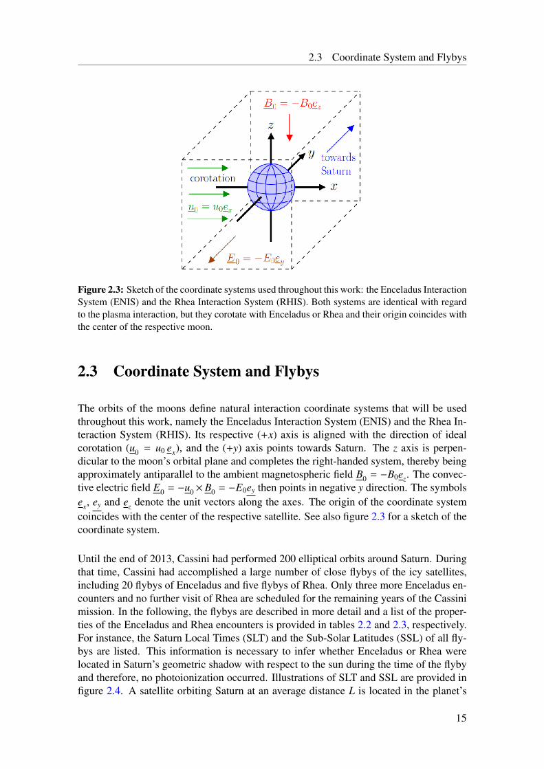
Figure 2.3: Sketch of the coordinate systems used throughout this work: the Enceladus InteractionSystem (ENIS) and the Rhea Interaction System (RHIS). Both systems are identical with regardto the plasma interaction, but they corotate with Enceladus or Rhea and their origin coincides withthe center of the respective moon.
2.3 Coordinate System and Flybys
The orbits of the moons define natural interaction coordinate systems that will be usedthroughout this work, namely the Enceladus Interaction System (ENIS) and the Rhea In-teraction System (RHIS). Its respective (+x) axis is aligned with the direction of idealcorotation (u0 = u0 ex), and the (+y) axis points towards Saturn. The z axis is perpen-dicular to the moon’s orbital plane and completes the right-handed system, thereby beingapproximately antiparallel to the ambient magnetospheric field B0 = −B0ez. The convec-tive electric field E0 = −u0 × B0 = −E0ey then points in negative y direction. The symbolsex, ey and ez denote the unit vectors along the axes. The origin of the coordinate systemcoincides with the center of the respective satellite. See also figure 2.3 for a sketch of thecoordinate system.
Until the end of 2013, Cassini had performed 200 elliptical orbits around Saturn. Duringthat time, Cassini had accomplished a large number of close flybys of the icy satellites,including 20 flybys of Enceladus and five flybys of Rhea. Only three more Enceladus en-counters and no further visit of Rhea are scheduled for the remaining years of the Cassinimission. In the following, the flybys are described in more detail and a list of the proper-ties of the Enceladus and Rhea encounters is provided in tables 2.2 and 2.3, respectively.For instance, the Saturn Local Times (SLT) and the Sub-Solar Latitudes (SSL) of all fly-bys are listed. This information is necessary to infer whether Enceladus or Rhea werelocated in Saturn’s geometric shadow with respect to the sun during the time of the flybyand therefore, no photoionization occurred. Illustrations of SLT and SSL are provided infigure 2.4. A satellite orbiting Saturn at an average distance L is located in the planet’s
15
2 The Magnetospheric Environment of Enceladus and Rhea
Suntowards
Saturn
SLT
23:00
01:00
(a)
Saturn
23:00 < SLT < 01:00
SSL
towards Sun
(b)
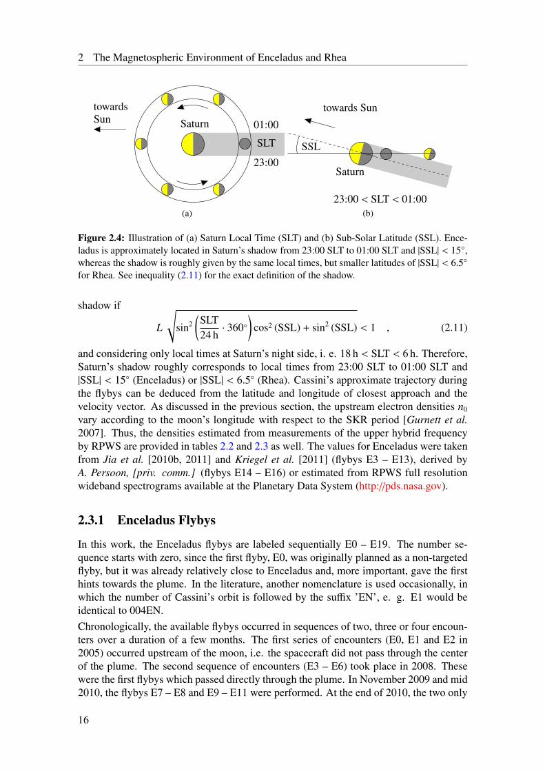
Figure 2.4: Illustration of (a) Saturn Local Time (SLT) and (b) Sub-Solar Latitude (SSL). Ence-ladus is approximately located in Saturn’s shadow from 23:00 SLT to 01:00 SLT and |SSL| < 15,whereas the shadow is roughly given by the same local times, but smaller latitudes of |SSL| < 6.5
for Rhea. See inequality (2.11) for the exact definition of the shadow.
shadow if
L
√sin2
(SLT24 h
· 360)
cos2 (SSL) + sin2 (SSL) < 1 , (2.11)
and considering only local times at Saturn’s night side, i. e. 18 h < SLT < 6 h. Therefore,Saturn’s shadow roughly corresponds to local times from 23:00 SLT to 01:00 SLT and|SSL| < 15 (Enceladus) or |SSL| < 6.5 (Rhea). Cassini’s approximate trajectory duringthe flybys can be deduced from the latitude and longitude of closest approach and thevelocity vector. As discussed in the previous section, the upstream electron densities n0
vary according to the moon’s longitude with respect to the SKR period [Gurnett et al.2007]. Thus, the densities estimated from measurements of the upper hybrid frequencyby RPWS are provided in tables 2.2 and 2.3 as well. The values for Enceladus were takenfrom Jia et al. [2010b, 2011] and Kriegel et al. [2011] (flybys E3 – E13), derived byA. Persoon, [priv. comm.] (flybys E14 – E16) or estimated from RPWS full resolutionwideband spectrograms available at the Planetary Data System (http://pds.nasa.gov).
2.3.1 Enceladus Flybys
In this work, the Enceladus flybys are labeled sequentially E0 – E19. The number se-quence starts with zero, since the first flyby, E0, was originally planned as a non-targetedflyby, but it was already relatively close to Enceladus and, more important, gave the firsthints towards the plume. In the literature, another nomenclature is used occasionally, inwhich the number of Cassini’s orbit is followed by the suffix ’EN’, e. g. E1 would beidentical to 004EN.Chronologically, the available flybys occurred in sequences of two, three or four encoun-ters over a duration of a few months. The first series of encounters (E0, E1 and E2 in2005) occurred upstream of the moon, i.e. the spacecraft did not pass through the centerof the plume. The second sequence of encounters (E3 – E6) took place in 2008. Thesewere the first flybys which passed directly through the plume. In November 2009 and mid2010, the flybys E7 – E8 and E9 – E11 were performed. At the end of 2010, the two only
16
2.3 Coordinate System and Flybys
north polar flybys E12 and E13 took place. Two additional series with three flybys each inautumn 2011 (E14 – E16) and spring 2012 (E17 – E19) complete the set of accomplishedflybys so far. Three further flybys (E20 – E22) will take place at the end of 2015.To better visualize the flyby trajectories, the flybys are grouped into five categories ac-cording to their trajectories and one additional category for the three future flybys:
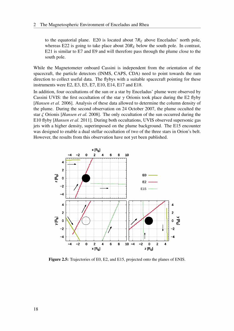
• There are three flybys which do not possess a counterpart with a similar trajectory,namely E0, E2, and E15. Their trajectories are displayed in fig. 2.5. The distantencounters E0 and E15 were directed towards Saturn and occurred far upstream ordownstream of Enceladus, respectively. Both trajectories were nearly parallel tothe equatorial plane. The closest approach of E0 took place north and upstream ofthe moon, while that of E15 was slightly south and more than 5RE downstream ofEnceladus. The E2 flyby was located upstream of the plume, possessing a south-to-north trajectory that is also oriented towards Saturn.
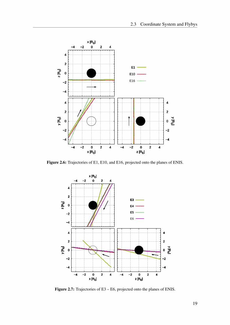
• The flybys E1, E10 and E16 possess similar trajectories which are parallel to theequatorial plane at z = −1.5RE, upstream of the plume and directed towards Sat-urn (see fig. 2.6). When crossing the (x, z)-plane, Cassini was located about 2RE
upstream of Enceladus.
• E3 – E6 constitute are series of highly inclined flybys during which Cassini passedsteep through the plume from downstream and north of Enceladus to upstream andsouth. The trajectories are shown in fig. 2.7. E3 features the highest inclination ofthese flybys and also included an inbound motion. The other three flybys possessednearly the same inclination, but E6 was located about 0.5RE further downstreamthan E4 and E5. The velocity during these encounters was a factor of two higherthan for the other flybys.
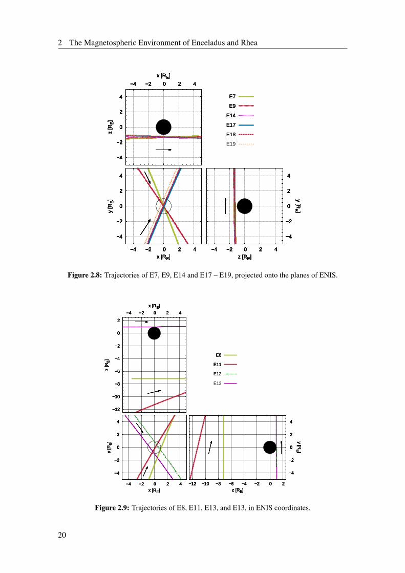
• Encounters E7, E9, E14 and E17 – E19 were all equatorial flybys parallel to themoon’s orbital plane at z = −1.5RE and crossed through the center of the plumewith a closest approach near Enceladus’ south pole. For E7 and E9, the trajectorieswere oriented from upstream to downstream and away from Saturn (outbound),while E14, E17, E18 and E19 were directed towards Saturn (see fig. 2.8). E14, E17and E18 possessed nearly identical trajectories. The E19 trajectory was parallel tothat of these three flybys, but located about 0.35RE further upstream.
• The remaining four encounters constitute of two pairs, E8/E11 and E12/E13 (seefig. 2.9). All four flybys were roughly parallel to the equatorial plane, althoughE11 features a small northward tilt of about 15. E8 and E11 were located far southof Enceladus at z = −7.3RE and z ≈ −11RE, respectively. E12 and E13 were bothnorth polar flybys and directed outbound. These two encounters possessed a nearlyidentical direction, but the closest approach of E12 was located about 1RE furtherdownstream than that of E13.
• No predicted trajectories are available for the future flybys E20 – E22. Their ap-proximate trajectories can, however, be constructed from the planned location ofclosest approach and the estimated velocity vector of Cassini at that point (see fig-ure 2.10). During all three planned encounters, Cassini is going to move parallel
17
2 The Magnetospheric Environment of Enceladus and Rhea
to the equatorial plane. E20 is located about 7RE above Enceladus’ north pole,whereas E22 is going to take place about 20RE below the south pole. In contrast,E21 is similar to E7 and E9 and will therefore pass through the plume close to thesouth pole.
While the Magnetometer onboard Cassini is independent from the orientation of thespacecraft, the particle detectors (INMS, CAPS, CDA) need to point towards the ramdirection to collect useful data. The flybys with a suitable spacecraft pointing for theseinstruments were E2, E3, E5, E7, E10, E14, E17 and E18.In addition, four occultations of the sun or a star by Enceladus’ plume were observed byCassini UVIS: the first occultation of the star γ Orionis took place during the E2 flyby[Hansen et al. 2006]. Analysis of these data allowed to determine the column density ofthe plume. During the second observation on 24 October 2007, the plume occulted thestar ζ Orionis [Hansen et al. 2008]. The only occultation of the sun occurred during theE10 flyby [Hansen et al. 2011]. During both occultations, UVIS observed supersonic gasjets with a higher density, superimposed on the plume background. The E15 encounterwas designed to enable a dual stellar occultation of two of the three stars in Orion’s belt.However, the results from this observation have not yet been published.
−4
−2
0
2
4
−4 −2 0 2 4 6 8 10
y [R
E]
x [RE]
−4
−2
0
2
4
−4 −2 0 2 4 6 8 10
y [R
E]
x [RE]
−4
−2
0
2
4
−4 −2 0 2 4 6 8 10
y [R
E]
x [RE]
−4
−2
0
2
4
−4 −2 0 2 4 6 8 10
y [R
E]
x [RE]−4 −2 0 2 4
−4
−2
0
2
4
y [RE ]
z [RE]−4 −2 0 2 4
−4
−2
0
2
4
y [RE ]
z [RE]−4 −2 0 2 4
−4
−2
0
2
4
y [RE ]
z [RE]−4 −2 0 2 4
−4
−2
0
2
4
y [RE ]
z [RE]
−4
−2
0
2
4
−4 −2 0 2 4 6 8 10
z [R
E]
x [RE]
−4
−2
0
2
4
−4 −2 0 2 4 6 8 10
z [R
E]
x [RE]
−4
−2
0
2
4
−4 −2 0 2 4 6 8 10
z [R
E]
x [RE]
−4
−2
0
2
4
−4 −2 0 2 4 6 8 10
z [R
E]
x [RE]
E0E0
E2
E0
E2
E15
Figure 2.5: Trajectories of E0, E2, and E15, projected onto the planes of ENIS.
18
2.3 Coordinate System and Flybys
−4
−2
0
2
4
−4 −2 0 2 4
y [R
E]
x [RE]
−4
−2
0
2
4
−4 −2 0 2 4
y [R
E]
x [RE]
−4
−2
0
2
4
−4 −2 0 2 4
y [R
E]
x [RE]
−4
−2
0
2
4
−4 −2 0 2 4
y [R
E]
x [RE]−4 −2 0 2 4
−4
−2
0
2
4
y [RE ]
z [RE]−4 −2 0 2 4
−4
−2
0
2
4
y [RE ]
z [RE]−4 −2 0 2 4
−4
−2
0
2
4
y [RE ]
z [RE]−4 −2 0 2 4
−4
−2
0
2
4
y [RE ]
z [RE]
−4
−2
0
2
4
−4 −2 0 2 4
z [R
E]
x [RE]
−4
−2
0
2
4
−4 −2 0 2 4
z [R
E]
x [RE]
−4
−2
0
2
4
−4 −2 0 2 4
z [R
E]
x [RE]
−4
−2
0
2
4
−4 −2 0 2 4
z [R
E]
x [RE]
E1E1
E10
E1
E10
E16
Figure 2.6: Trajectories of E1, E10, and E16, projected onto the planes of ENIS.
−4
−2
0
2
4
−4 −2 0 2 4
y [R
E]
x [RE]
−4
−2
0
2
4
−4 −2 0 2 4
y [R
E]
x [RE]
−4
−2
0
2
4
−4 −2 0 2 4
y [R
E]
x [RE]
−4
−2
0
2
4
−4 −2 0 2 4
y [R
E]
x [RE]
−4
−2
0
2
4
−4 −2 0 2 4
y [R
E]
x [RE]−4 −2 0 2 4
−4
−2
0
2
4
y [RE ]
z [RE]−4 −2 0 2 4
−4
−2
0
2
4
y [RE ]
z [RE]−4 −2 0 2 4
−4
−2
0
2
4
y [RE ]
z [RE]−4 −2 0 2 4
−4
−2
0
2
4
y [RE ]
z [RE]−4 −2 0 2 4
−4
−2
0
2
4
y [RE ]
z [RE]
−4
−2
0
2
4
−4 −2 0 2 4
z [R
E]
x [RE]
−4
−2
0
2
4
−4 −2 0 2 4
z [R
E]
x [RE]
−4
−2
0
2
4
−4 −2 0 2 4
z [R
E]
x [RE]
−4
−2
0
2
4
−4 −2 0 2 4
z [R
E]
x [RE]
−4
−2
0
2
4
−4 −2 0 2 4
z [R
E]
x [RE]
E3E3
E4
E3
E4
E5
E3
E4
E5
E6
Figure 2.7: Trajectories of E3 – E6, projected onto the planes of ENIS.
19
2 The Magnetospheric Environment of Enceladus and Rhea
−4
−2
0
2
4
−4 −2 0 2 4
y [R
E]
x [RE]
−4
−2
0
2
4
−4 −2 0 2 4
y [R
E]
x [RE]
−4
−2
0
2
4
−4 −2 0 2 4
y [R
E]
x [RE]
−4
−2
0
2
4
−4 −2 0 2 4
y [R
E]
x [RE]
−4
−2
0
2
4
−4 −2 0 2 4
y [R
E]
x [RE]
−4
−2
0
2
4
−4 −2 0 2 4
y [R
E]
x [RE]
−4
−2
0
2
4
−4 −2 0 2 4
y [R
E]
x [RE]−4 −2 0 2 4
−4
−2
0
2
4
y [RE ]
z [RE]−4 −2 0 2 4
−4
−2
0
2
4
y [RE ]
z [RE]−4 −2 0 2 4
−4
−2
0
2
4
y [RE ]
z [RE]−4 −2 0 2 4
−4
−2
0
2
4
y [RE ]
z [RE]−4 −2 0 2 4
−4
−2
0
2
4
y [RE ]
z [RE]−4 −2 0 2 4
−4
−2
0
2
4
y [RE ]
z [RE]−4 −2 0 2 4
−4
−2
0
2
4
y [RE ]
z [RE]
−4
−2
0
2
4
−4 −2 0 2 4
z [R
E]
x [RE]
−4
−2
0
2
4
−4 −2 0 2 4
z [R
E]
x [RE]
−4
−2
0
2
4
−4 −2 0 2 4
z [R
E]
x [RE]
−4
−2
0
2
4
−4 −2 0 2 4
z [R
E]
x [RE]
−4
−2
0
2
4
−4 −2 0 2 4
z [R
E]
x [RE]
−4
−2
0
2
4
−4 −2 0 2 4
z [R
E]
x [RE]
−4
−2
0
2
4
−4 −2 0 2 4
z [R
E]
x [RE]
E7E7
E9
E7
E9
E14
E7
E9
E14
E17
E7
E9
E14
E17
E18
E7
E9
E14
E17
E18
E19
Figure 2.8: Trajectories of E7, E9, E14 and E17 – E19, projected onto the planes of ENIS.
−4
−2
0
2
4
−4 −2 0 2 4
y [R
E]
x [RE]
−4
−2
0
2
4
−4 −2 0 2 4
y [R
E]
x [RE]
−4
−2
0
2
4
−4 −2 0 2 4
y [R
E]
x [RE]
−4
−2
0
2
4
−4 −2 0 2 4
y [R
E]
x [RE]
−4
−2
0
2
4
−4 −2 0 2 4
y [R
E]
x [RE]
−12 −10 −8 −6 −4 −2 0 2
−4
−2
0
2
4
y [RE ]
z [RE]−12 −10 −8 −6 −4 −2 0 2
−4
−2
0
2
4
y [RE ]
z [RE]−12 −10 −8 −6 −4 −2 0 2
−4
−2
0
2
4
y [RE ]
z [RE]−12 −10 −8 −6 −4 −2 0 2
−4
−2
0
2
4
y [RE ]
z [RE]−12 −10 −8 −6 −4 −2 0 2
−4
−2
0
2
4
y [RE ]
z [RE]
−12
−10
−8
−6
−4
−2
0
2
−4 −2 0 2 4
z [R
E]
x [RE]
−12
−10
−8
−6
−4
−2
0
2
−4 −2 0 2 4
z [R
E]
x [RE]
−12
−10
−8
−6
−4
−2
0
2
−4 −2 0 2 4
z [R
E]
x [RE]
−12
−10
−8
−6
−4
−2
0
2
−4 −2 0 2 4
z [R
E]
x [RE]
−12
−10
−8
−6
−4
−2
0
2
−4 −2 0 2 4
z [R
E]
x [RE]
E8E8
E11
E8
E11
E12
E8
E11
E12
E13
Figure 2.9: Trajectories of E8, E11, E13, and E13, in ENIS coordinates.
20
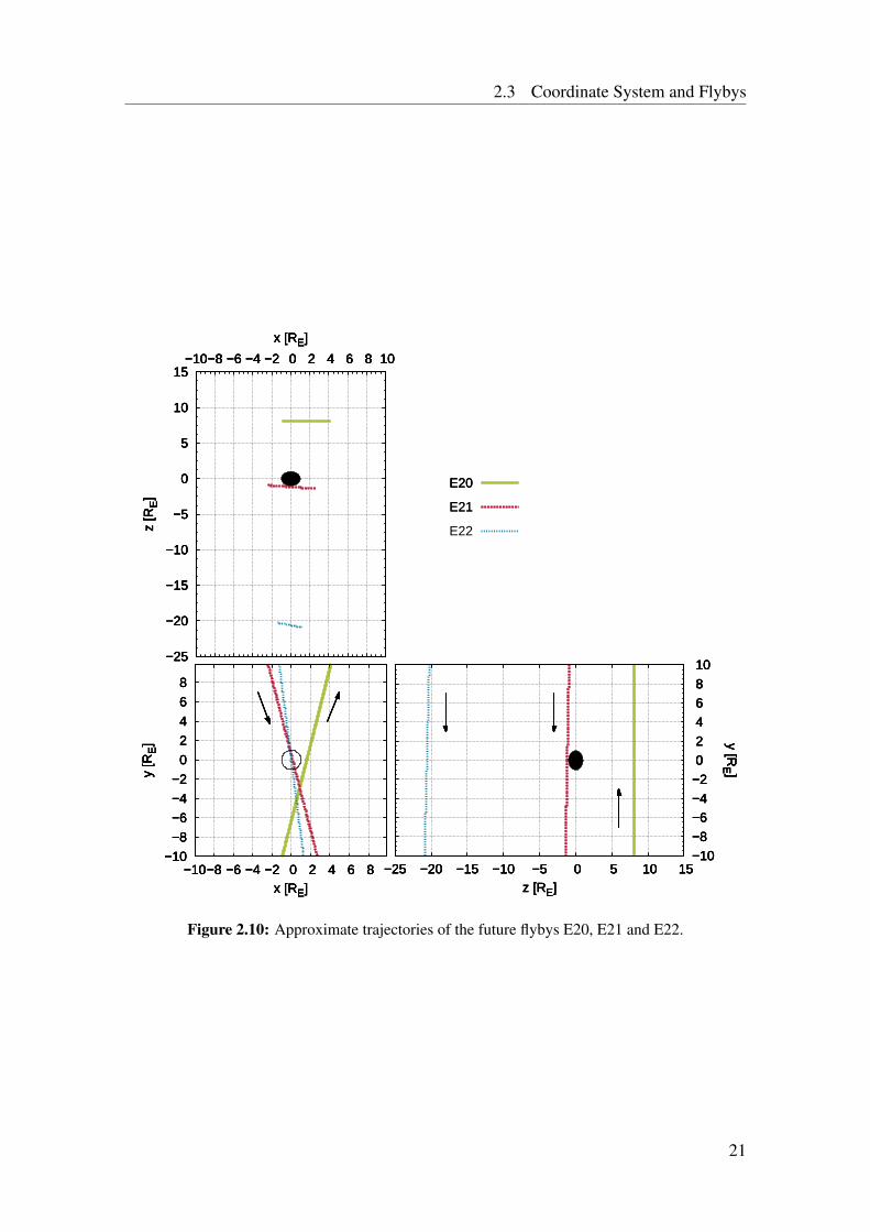
2.3 Coordinate System and Flybys
−10
−8
−6
−4
−2
0
2
4
6
8
−10−8 −6 −4 −2 0 2 4 6 8
y [R
E]
x [RE]
−10
−8
−6
−4
−2
0
2
4
6
8
−10−8 −6 −4 −2 0 2 4 6 8
y [R
E]
x [RE]
−10
−8
−6
−4
−2
0
2
4
6
8
−10−8 −6 −4 −2 0 2 4 6 8
y [R
E]
x [RE]
−10
−8
−6
−4
−2
0
2
4
6
8
−10−8 −6 −4 −2 0 2 4 6 8
y [R
E]
x [RE]
−25 −20 −15 −10 −5 0 5 10 15−10−8
−6−4−2
0 2 4 6
8 10
y [RE ]
z [RE]−25 −20 −15 −10 −5 0 5 10 15
−10−8
−6−4−2
0 2 4 6
8 10
y [RE ]
z [RE]−25 −20 −15 −10 −5 0 5 10 15
−10−8
−6−4−2
0 2 4 6
8 10
y [RE ]
z [RE]−25 −20 −15 −10 −5 0 5 10 15
−10−8
−6−4−2
0 2 4 6
8 10
y [RE ]
z [RE]
−25
−20
−15
−10
−5
0
5
10
15−10−8 −6 −4 −2 0 2 4 6 8 10
z [R
E]
x [RE]
−25
−20
−15
−10
−5
0
5
10
15−10−8 −6 −4 −2 0 2 4 6 8 10
z [R
E]
x [RE]
−25
−20
−15
−10
−5
0
5
10
15−10−8 −6 −4 −2 0 2 4 6 8 10
z [R
E]
x [RE]
−25
−20
−15
−10
−5
0
5
10
15−10−8 −6 −4 −2 0 2 4 6 8 10
z [R
E]
x [RE]
E20E20
E21
E20
E21
E22
Figure 2.10: Approximate trajectories of the future flybys E20, E21 and E22.
21
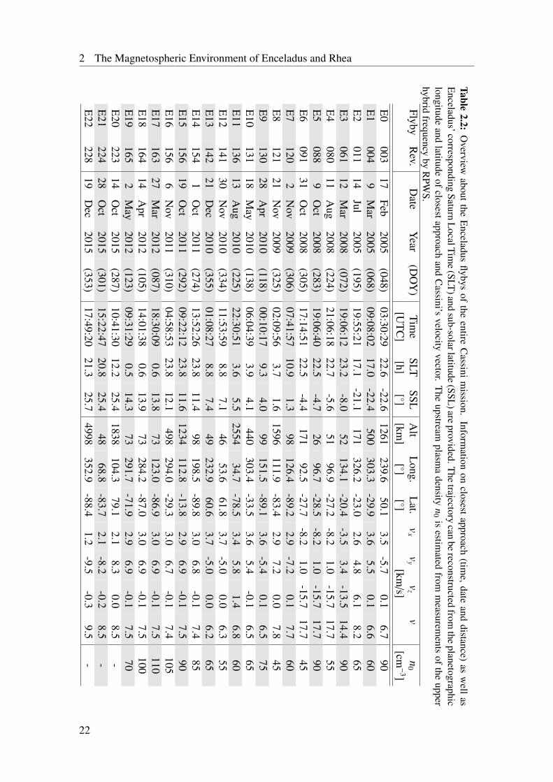
2 The Magnetospheric Environment of Enceladus and Rhea
Table2.2:
Overview
aboutthe
Enceladus
flybysof
theentire
Cassini
mission.
Information
onclosest
approach(tim
e,date
anddistance)
asw
ellas
Enceladus’corresponding
SaturnL
ocalTime
(SLT)and
sub-solarlatitude(SSL
)areprovided.T
hetrajectory
canbe
reconstructedfrom
theplanetographic
longitudeand
latitudeof
closestapproachand
Cassini’s
velocityvector.
The
upstreamplasm
adensity
n0
isestim
atedfrom
measurem
entsof
theupper
hybridfrequency
byR
PWS.
FlybyR
ev.D
ateY
ear(D
OY
)Tim
eSLT
SSLA
ltL
ong.L
at.v
xv
yv
zv
n0
[UT
C]
[h][]
[km]
[]
[]
[km/s]
[cm−
3]E
0003
17Feb
2005(048)
03:30:2922.6
-22.61261
239.650.1
3.5-5.7
0.16.7
90E
1004
9M
ar2005
(068)09:08:02
17.0-22.4
500303.3
-29.93.6
5.50.1
6.660
E2
01114
Jul2005
(195)19:55:21
17.1-21.1
171326.2
-23.02.6
4.86.1
8.265
E3
06112
Mar
2008(072)
19:06:1223.2
-8.052
134.1-20.4
-3.53.4
-13.514.4
90E
4080
11A
ug2008
(224)21:06:18
22.7-5.6
5196.9
-27.2-8.2
1.0-15.7
17.755
E5
0889
Oct
2008(283)
19:06:4022.5
-4.726
96.7-28.5
-8.21.0
-15.717.7
90E
6091
31O
ct2008
(305)17:14:51
22.5-4.4
17192.5
-27.7-8.2
1.0-15.7
17.745
E7
1202
Nov
2009(306)
07:41:5710.9
1.398
126.4-89.2
2.9-7.2
0.17.7
60E
8121
21N
ov2009
(325)02:09:56
3.71.6
1596111.9
-83.42.9
7.20.0
7.845
E9
13028
Apr
2010(118)
00:10:179.3
4.099
151.5-89.1
3.6-5.4
0.16.5
75E
10131
18M
ay2010
(138)06:04:39
3.94.1
440303.4
-33.53.6
5.4-0.1
6.565
E11
13613
Aug
2010(225)
22:30:513.6
5.52554
34.7-78.5
3.45.8
1.46.8
60E
12141
30N
ov2010
(334)11:53:59
8.87.1
4653.6
61.83.7
-5.00.0
6.355
E13
14221
Dec
2010(355)
01:08:278.8
7.449
232.960.6
3.7-5.0
0.06.2
65E
14154
1O
ct2011
(274)13:52:26
23.811.4
98198.5
-89.83.0
6.8-0.1
7.485
E15
15619
Oct
2011(292)
09:22:1223.8
11.61234
112.8-13.8
2.96.9
-0.17.5
90E
16156
6N
ov2011
(310)04:58:53
23.812.1
498294.0
-29.33.0
6.7-0.1
7.4105
E17
16327
Mar
2012(087)
18:30:090.6
13.873
123.0-86.9
3.06.9
-0.17.5
110E
18164
14A
pr2012
(105)14:01:38
0.613.9
73284.2
-87.03.0
6.9-0.1
7.5100
E19
1652
May
2012(123)
09:31:290.5
14.373
291.7-71.9
2.96.9
-0.17.5
70E
20223
14O
ct2015
(287)10:41:30
12.225.4
1838104.3
79.12.1
8.30.0
8.5-
E21
22428
Oct
2015(301)
15:22:4720.8
25.448
68.8-83.7
2.1-8.2
-0.28.5
-E
22228
19D
ec2015
(353)17:49:20
21.325.7
4998352.9
-88.41.2
-9.5-0.3
9.5-
22
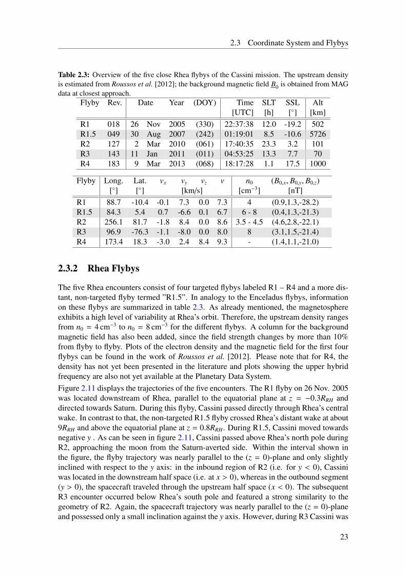
2.3 Coordinate System and Flybys
Table 2.3: Overview of the five close Rhea flybys of the Cassini mission. The upstream densityis estimated from Roussos et al. [2012]; the background magnetic field B0 is obtained from MAGdata at closest approach.
Flyby Rev. Date Year (DOY) Time SLT SSL Alt[UTC] [h] [] [km]
R1 018 26 Nov 2005 (330) 22:37:38 12.0 -19.2 502R1.5 049 30 Aug 2007 (242) 01:19:01 8.5 -10.6 5726R2 127 2 Mar 2010 (061) 17:40:35 23.3 3.2 101R3 143 11 Jan 2011 (011) 04:53:25 13.3 7.7 70R4 183 9 Mar 2013 (068) 18:17:28 1.1 17.5 1000
Flyby Long. Lat. vx vy vz v n0 (B0,x, B0,y, B0,z)[] [] [km/s] [cm−3] [nT]
R1 88.7 -10.4 -0.1 7.3 0.0 7.3 4 (0.9,1.3,-28.2)R1.5 84.3 5.4 0.7 -6.6 0.1 6.7 6 - 8 (0.4,1.3,-21.3)R2 256.1 81.7 -1.8 8.4 0.0 8.6 3.5 - 4.5 (4.6,2.8,-22.1)R3 96.9 -76.3 -1.1 -8.0 0.0 8.0 8 (3.1,1.5,-21.4)R4 173.4 18.3 -3.0 2.4 8.4 9.3 - (1.4,1.1,-21.0)
2.3.2 Rhea Flybys
The five Rhea encounters consist of four targeted flybys labeled R1 – R4 and a more dis-tant, non-targeted flyby termed ”R1.5”. In analogy to the Enceladus flybys, informationon these flybys are summarized in table 2.3. As already mentioned, the magnetosphereexhibits a high level of variability at Rhea’s orbit. Therefore, the upstream density rangesfrom n0 = 4 cm−3 to n0 = 8 cm−3 for the different flybys. A column for the backgroundmagnetic field has also been added, since the field strength changes by more than 10%from flyby to flyby. Plots of the electron density and the magnetic field for the first fourflybys can be found in the work of Roussos et al. [2012]. Please note that for R4, thedensity has not yet been presented in the literature and plots showing the upper hybridfrequency are also not yet available at the Planetary Data System.Figure 2.11 displays the trajectories of the five encounters. The R1 flyby on 26 Nov. 2005was located downstream of Rhea, parallel to the equatorial plane at z = −0.3RRH anddirected towards Saturn. During this flyby, Cassini passed directly through Rhea’s centralwake. In contrast to that, the non-targeted R1.5 flyby crossed Rhea’s distant wake at about9RRH and above the equatorial plane at z = 0.8RRH. During R1.5, Cassini moved towardsnegative y . As can be seen in figure 2.11, Cassini passed above Rhea’s north pole duringR2, approaching the moon from the Saturn-averted side. Within the interval shown inthe figure, the flyby trajectory was nearly parallel to the (z = 0)-plane and only slightlyinclined with respect to the y axis: in the inbound region of R2 (i.e. for y < 0), Cassiniwas located in the downstream half space (i.e. at x > 0), whereas in the outbound segment(y > 0), the spacecraft traveled through the upstream half space (x < 0). The subsequentR3 encounter occurred below Rhea’s south pole and featured a strong similarity to thegeometry of R2. Again, the spacecraft trajectory was nearly parallel to the (z = 0)-planeand possessed only a small inclination against the y axis. However, during R3 Cassini was
23
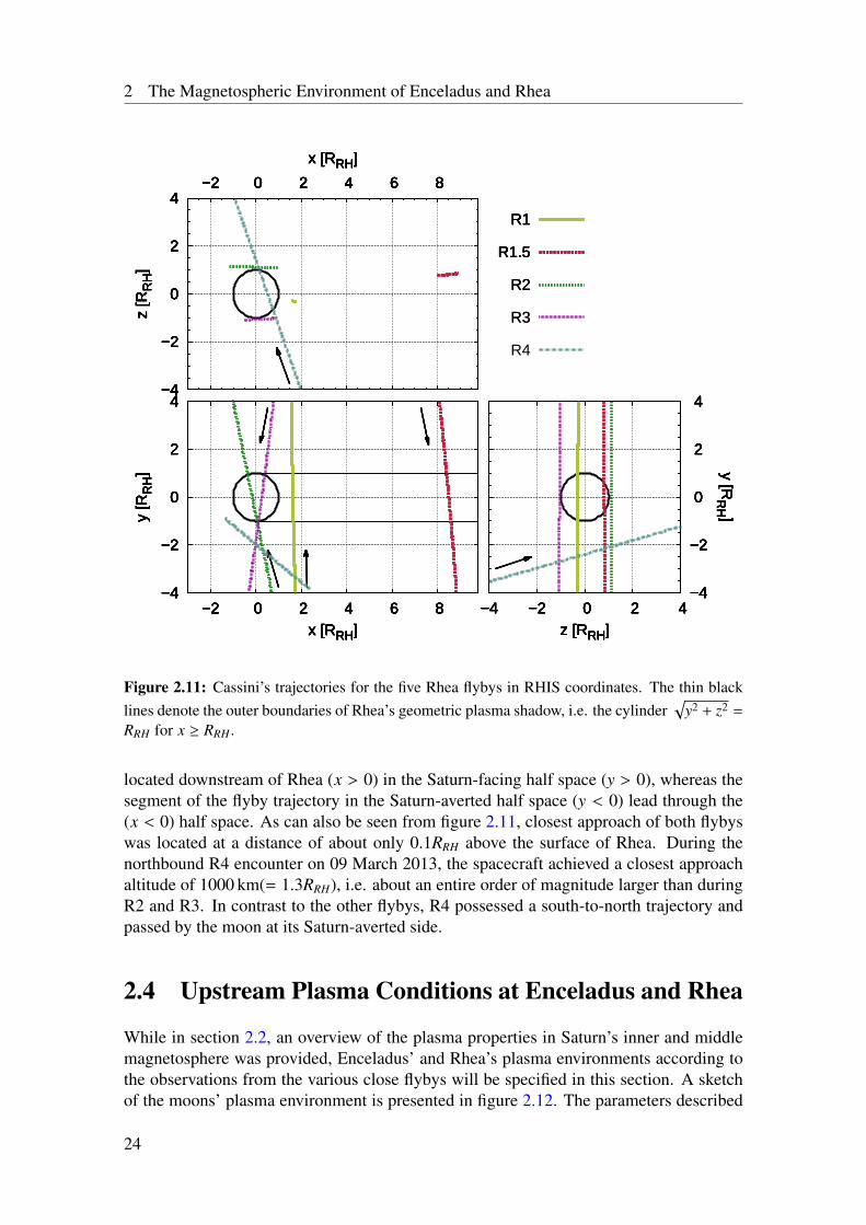
2 The Magnetospheric Environment of Enceladus and Rhea
−4
−2
0
2
4
−2 0 2 4 6 8
y [R
RH
]
x [RRH]
−4
−2
0
2
4
−2 0 2 4 6 8
y [R
RH
]
x [RRH]
−4
−2
0
2
4
−2 0 2 4 6 8
y [R
RH
]
x [RRH]
−4
−2
0
2
4
−2 0 2 4 6 8
y [R
RH
]
x [RRH]
−4
−2
0
2
4
−2 0 2 4 6 8
y [R
RH
]
x [RRH]
−4
−2
0
2
4
−2 0 2 4 6 8
y [R
RH
]
x [RRH]−4 −2 0 2 4
−4
−2
0
2
4
y [RR
H ]
z [RRH]−4 −2 0 2 4
−4
−2
0
2
4
y [RR
H ]
z [RRH]−4 −2 0 2 4
−4
−2
0
2
4
y [RR
H ]
z [RRH]−4 −2 0 2 4
−4
−2
0
2
4
y [RR
H ]
z [RRH]−4 −2 0 2 4
−4
−2
0
2
4
y [RR
H ]
z [RRH]−4 −2 0 2 4
−4
−2
0
2
4
y [RR
H ]
z [RRH]
−4
−2
0
2
4−2 0 2 4 6 8
z [R
RH
]x [RRH]
−4
−2
0
2
4−2 0 2 4 6 8
z [R
RH
]x [RRH]
−4
−2
0
2
4−2 0 2 4 6 8
z [R
RH
]x [RRH]
−4
−2
0
2
4−2 0 2 4 6 8
z [R
RH
]x [RRH]
−4
−2
0
2
4−2 0 2 4 6 8
z [R
RH
]x [RRH]
−4
−2
0
2
4−2 0 2 4 6 8
z [R
RH
]x [RRH]
R1R1
R1.5
R1
R1.5
R2
R1
R1.5
R2
R3
R1
R1.5
R2
R3
R4
Figure 2.11: Cassini’s trajectories for the five Rhea flybys in RHIS coordinates. The thin blacklines denote the outer boundaries of Rhea’s geometric plasma shadow, i.e. the cylinder
√y2 + z2 =
RRH for x ≥ RRH .
located downstream of Rhea (x > 0) in the Saturn-facing half space (y > 0), whereas thesegment of the flyby trajectory in the Saturn-averted half space (y < 0) lead through the(x < 0) half space. As can also be seen from figure 2.11, closest approach of both flybyswas located at a distance of about only 0.1RRH above the surface of Rhea. During thenorthbound R4 encounter on 09 March 2013, the spacecraft achieved a closest approachaltitude of 1000 km(= 1.3RRH), i.e. about an entire order of magnitude larger than duringR2 and R3. In contrast to the other flybys, R4 possessed a south-to-north trajectory andpassed by the moon at its Saturn-averted side.
2.4 Upstream Plasma Conditions at Enceladus and Rhea
While in section 2.2, an overview of the plasma properties in Saturn’s inner and middlemagnetosphere was provided, Enceladus’ and Rhea’s plasma environments according tothe observations from the various close flybys will be specified in this section. A sketchof the moons’ plasma environment is presented in figure 2.12. The parameters described
24
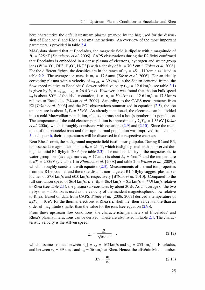
2.4 Upstream Plasma Conditions at Enceladus and Rhea
here characterize the default upstream plasma (marked by the hat) used for the discus-sion of Enceladus’ and Rhea’s plasma interactions. An overview of the most importantparameters is provided in table 2.4.MAG data showed that at Enceladus, the magnetic field is dipolar with a magnitude ofB0 = 325 nT [Dougherty et al. 2006]. CAPS observations during the E2 flyby confirmedthat Enceladus is embedded in a dense plasma of electrons, hydrogen and water groupions (W+=O+, OH+, H2O+, H3O+) with a density of n0 = 70.5 cm−3 [Tokar et al. 2006].For the different flybys, the densities are in the range of n0 = 45 − 110 cm−3 as listed intable 2.2. The average ion mass is mi = 17.6 amu [Tokar et al. 2006]. For an ideallycorotating plasma with a velocity of u0,Sat. = 39 km/s in the Saturn-centered frame, theflow speed relative to Enceladus’ slower orbital velocity (vE = 12.6 km/s, see table 2.1)is given by u0 = u0,Sat. − vE = 26.4 km/s. However, it was found that the ion bulk speedu0 is about 80% of the ideal coratation, i. e. u0 = 30.4 km/s − 12.6 km/s = 17.8 km/srelative to Enceladus [Wilson et al. 2009]. According to the CAPS measurements fromE2 [Tokar et al. 2006] and the SOI observations summarized in equation (2.3), the iontemperature is about kBTi = 35 eV. As already mentioned, the electrons can be dividedinto a cold Maxwellian population, photoelectrons and a hot (suprathermal) population.The temperature of the cold electron population is approximately kBTec = 1.35 eV [Tokaret al. 2006], which is roughly consistent with equations (2.9) and (2.10). Since the treat-ment of the photoelectrons and the suprathermal population was improved from chapter5 to chapter 6, their temperatures will be discussed in the respective chapters.Near Rhea’s orbit, the background magnetic field is still nearly dipolar. During R2 and R3,it possessed a magnitude of about B0 = 21 nT, which is slightly smaller than observed dur-ing the initial R1 flyby in 2005 (see table 2.3). The number density of the magnetosphericwater group ions (average mass mi = 17 amu) is about n0 = 6 cm−3 and the temperatureis kTi = 200 eV (cf. table 1 in Khurana et al. [2008] and table 2 in Wilson et al. [2009]),which is roughly consistent with equation (2.3). Measurements of thermal ion propertiesfrom the R1 encounter and the more distant, non-targeted R1.5 flyby suggest plasma ve-locities of 57.6 km/s and 60.0 km/s, respectively [Wilson et al. 2010]. Compared to thefull corotation speed of 86.4 km/s, i. e. u0 = 86.4 km/s − 8.5 km/s = 77.9 km/s relativeto Rhea (see table 2.1), the plasma sub-corotates by about 30%. As an average of the twoflybys, u0 = 50 km/s is used as the velocity of the incident magnetospheric flow relativeto Rhea. Based on data from CAPS, Sittler et al. [2006, 2007] derived a temperature ofkBTec = 10 eV for the thermal electrons at Rhea’s L-shell, i.e. their value is more than anorder of magnitude smaller than the value for the ions (see equation (2.9)).From these upstream flow conditions, the characteristic parameters of Enceladus’ andRhea’s plasma interactions can be derived. These are also listed in table 2.4. The charac-teristic velocity is the Alfvén speed,
vA =B0
õ0nimi
, (2.12)
which assumes values between |vA| = vA = 162 km/s and vA = 253 km/s at Enceladus,and between vA = 39 km/s and vA = 56 km/s at Rhea. Hence, the alfvénic Mach number
MA =u0
vA(2.13)
25
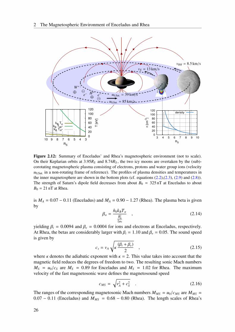
2 The Magnetospheric Environment of Enceladus and Rhea
0
20
40
60
80
100
120
3 4 5 6 7 8 9 10
n [
cm
-3]
RS
density
3 4 5 6 7 8 9 10 0
20
40
60
80
100
120
T [eV
]
RS
kB TekB TW
+
kB TH+
W+
H+e− e−
u0,Sat. = 85 km/s
u0,Sat. = 39 km/s
vE = 13 km/svRH = 8.5 km/s
Figure 2.12: Summary of Enceladus’ and Rhea’s magnetospheric environment (not to scale).On their Keplarian orbits at 3.95RS and 8.74RS , the two icy moons are overtaken by the (sub)-corotating magnetospheric plasma consisting of electrons, protons and water group ions (velocityu0,Sat. in a non-rotating frame of reference). The profiles of plasma densities and temperatures inthe inner magnetosphere are shown in the bottom plots (cf. equations (2.2),(2.3), (2.9) and (2.8)).The strength of Saturn’s dipole field decreases from about B0 = 325 nT at Enceladus to aboutB0 = 21 nT at Rhea.
is MA = 0.07 − 0.11 (Enceladus) and MA = 0.90 − 1.27 (Rhea). The plasma beta is givenby
βα =n0kBTα
B20
2µ0
, (2.14)
yielding βi = 0.0094 and βe = 0.0004 for ions and electrons at Enceladus, respectively.At Rhea, the betas are considerably larger with βi = 1.10 and βe = 0.05. The sound speedis given by
cs = vA
√κ
(βi + βe)2
, (2.15)
where κ denotes the adiabatic exponent with κ = 2. This value takes into account that themagnetic field reduces the degrees of freedom to two. The resulting sonic Mach numbersMS = u0/cS are MS = 0.89 for Enceladus and MS = 1.02 for Rhea. The maximumvelocity of the fast magnetosonic wave defines the magnetosound speed
cMS =
√v2
A + c2S . (2.16)
The ranges of the corresponding magnetosonic Mach numbers MMS = u0/cMS are MMS =
0.07 − 0.11 (Enceladus) and MMS = 0.68 − 0.80 (Rhea). The length scales of Rhea’s
26
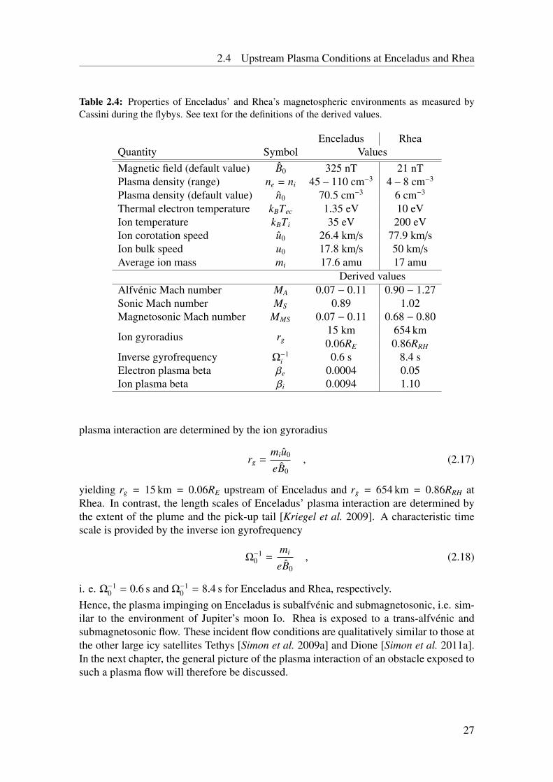
2.4 Upstream Plasma Conditions at Enceladus and Rhea
Table 2.4: Properties of Enceladus’ and Rhea’s magnetospheric environments as measured byCassini during the flybys. See text for the definitions of the derived values.
Enceladus RheaQuantity Symbol ValuesMagnetic field (default value) B0 325 nT 21 nTPlasma density (range) ne = ni 45 – 110 cm−3 4 – 8 cm−3
Plasma density (default value) n0 70.5 cm−3 6 cm−3
Thermal electron temperature kBTec 1.35 eV 10 eVIon temperature kBTi 35 eV 200 eVIon corotation speed u0 26.4 km/s 77.9 km/sIon bulk speed u0 17.8 km/s 50 km/sAverage ion mass mi 17.6 amu 17 amu
Derived valuesAlfvénic Mach number MA 0.07 − 0.11 0.90 − 1.27Sonic Mach number MS 0.89 1.02Magnetosonic Mach number MMS 0.07 − 0.11 0.68 − 0.80
Ion gyroradius rg15 km 654 km0.06RE 0.86RRH
Inverse gyrofrequency Ω−1i 0.6 s 8.4 s
Electron plasma beta βe 0.0004 0.05Ion plasma beta βi 0.0094 1.10
plasma interaction are determined by the ion gyroradius
rg =miu0
eB0, (2.17)
yielding rg = 15 km = 0.06RE upstream of Enceladus and rg = 654 km = 0.86RRH atRhea. In contrast, the length scales of Enceladus’ plasma interaction are determined bythe extent of the plume and the pick-up tail [Kriegel et al. 2009]. A characteristic timescale is provided by the inverse ion gyrofrequency
Ω−10 =
mi
eB0, (2.18)
i. e. Ω−10 = 0.6 s and Ω−1
0 = 8.4 s for Enceladus and Rhea, respectively.Hence, the plasma impinging on Enceladus is subalfvénic and submagnetosonic, i.e. sim-ilar to the environment of Jupiter’s moon Io. Rhea is exposed to a trans-alfvénic andsubmagnetosonic flow. These incident flow conditions are qualitatively similar to those atthe other large icy satellites Tethys [Simon et al. 2009a] and Dione [Simon et al. 2011a].In the next chapter, the general picture of the plasma interaction of an obstacle exposed tosuch a plasma flow will therefore be discussed.
27

3 Basics of Enceladus’ and Rhea’sPlasma Interaction
In this chapter, the foundations of the understanding of the plasma structures arisingfrom the interaction of Saturn’s magnetospheric plasma with Enceladus and Rhea willbe laid. Since Rhea does not possess a significant ionosphere1, the structures resultingfrom plasma absorption at the surface of an icy moon will be briefly described in section3.1. Moreover, previous studies of Rhea’s interaction are summarized. The main part ofthis chapter deals, however, with the theoretical background of the Alfvén wing, i.e. themagnetic field structures caused by the subalfvénic plasma interaction of a conductingobstacle (section 3.2). Since it will be demonstrated within this thesis that the plasmastructures of both, Enceladus and Rhea, reveal new aspects of the properties and the gen-eration of an Alfvén wing, its analytical description will be presented in some detail. Insection 3.4, an overview of the state of knowledge on Enceladus’ plasma interaction apartfrom the results presented in this thesis is provided. In particular, the open questionswhich are addressed in this work will be pointed out in section 3.5.
3.1 Interaction of an Inert Moon
For any planetary body that possesses neither an intrinsic magnetic field nor a substantialionosphere, the impinging plasma is simply absorbed at the surface of the body. This ab-sorption results in the formation of an extended density cavity in the downstream region.The shape of this density cavity, its refilling and the associated currents and magneticfield structures have already been analyzed by a number of authors. The plasma environ-ments of the icy moons Rhea and Tethys have been studied by e.g., Khurana et al. [2008],Roussos et al. [2008a] and Simon et al. [2009b], whereas the interaction of Enceladus’absorbing body has been analyzed in a preceding study [Kriegel et al. 2009].Perpendicular to the magnetic field, the density cavity is approximately restricted to thewidth of the moons’ geometric shadow with respect to the plasma flow. Parallel to themagnetic field, the depletion region expands along the magnetic field lines and forms atwo-dimensional, symmetric cone (cf. fig. 1 of Roussos et al. [2008a]). The structure ofthe wake region can be explained from different points of view:The most illustrative description is provided by the motion of single particles, cf. figure3.1. Due to the high thermal velocity of the upstream plasma (vth & u0), many particles
1The magnetic significance of Rhea’s ionosphere is discussed in chapter 7.
29
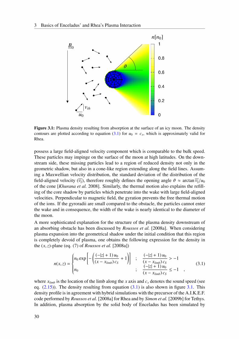
3 Basics of Enceladus’ and Rhea’s Plasma Interaction
ϑ
B0
n[n0]
u0
vth
Figure 3.1: Plasma density resulting from absorption at the surface of an icy moon. The densitycontours are plotted according to equation (3.1) for u0 = cs, which is approximately valid forRhea.
possess a large field-aligned velocity component which is comparable to the bulk speed.These particles may impinge on the surface of the moon at high latitudes. On the down-stream side, these missing particles lead to a region of reduced density not only in thegeometric shadow, but also in a cone-like region extending along the field lines. Assum-ing a Maxwellian velocity distribution, the standard deviation of the distribution of thefield-aligned velocity (v‖), therefore roughly defines the opening angle ϑ ≈ arctan v‖/u0
of the cone [Khurana et al. 2008]. Similarly, the thermal motion also explains the refill-ing of the core shadow by particles which penetrate into the wake with large field-alignedvelocities. Perpendicular to magnetic field, the gyration prevents the free thermal motionof the ions. If the gyroradii are small compared to the obstacle, the particles cannot enterthe wake and in consequence, the width of the wake is nearly identical to the diameter ofthe moon.A more sophisticated explanation for the structure of the plasma density downstream ofan absorbing obstacle has been discussed by Roussos et al. [2008a]. When consideringplasma expansion into the geometrical shadow under the initial condition that this regionis completely devoid of plasma, one obtains the following expression for the density inthe (x, z)-plane (eq. (7) of Roussos et al. [2008a])
n(x, z) =
n0 exp
[−
((−|z| + 1) u0
(x − xlimb) cS+ 1
)];
(−|z| + 1) u0
(x − xlimb) cS> −1
n0 ;(−|z| + 1) u0
(x − xlimb) cS≤ −1 ,
(3.1)
where xlimb is the location of the limb along the x axis and cs denotes the sound speed (seeeq. (2.15)). The density resulting from equation (3.1) is also shown in figure 3.1. Thisdensity profile is in agreement with hybrid simulations with the precursor of the A.I.K.E.F.code performed by Roussos et al. [2008a] for Rhea and by Simon et al. [2009b] for Tethys.In addition, plasma absorption by the solid body of Enceladus has been simulated by
30
3.1 Interaction of an Inert Moon
means of the A.I.K.E.F. in a preceding study [Kriegel et al. 2009].A third point of view to analyze the structure of the wake is given by the superposition ofthe magnetohydrodamic modes launched at the surface of the obstacle [Neubauer 1998].Such an analysis has been carried out by Wiehle et al. [2011] for the Earth moon and byVernisse et al. [2013] in a more general study of the interaction of an absorbing obstacle.A peculiar feature of Rhea’s plasma interaction stems from the large gyroradii of the mag-netospheric upstream ions which are almost comparable to the radius of Rhea (cf. table2.4). Therefore, the absorption of magnetospheric particles at the moon’s surface is ex-pected to possess a pronounced asymmetry with respect to the direction of the convectiveelectric field. In chapter 7, it shall be discussed how the large gyroradii of the ions imping-ing on Rhea modify the shape of the plasma wake. At Tethys (rg = 30.9 km = 0.06RT )and Dione (rg = 92.3 km = 0.16RD), asymmetries due to finite gyroradius effects are ex-pected to play a far less important role (where R j, j = T,D, denotes the respective satelliteradius, values of rg derived from table 1 in Khurana et al. [2008]).The discussion above focused only on the ions. Due to the higher mobility, the electronsrefill the wake more quickly. To maintain quasi-neutrality, the ions are dragged into thewake by ambipolar fields. On scales larger than the Debye length, these processes canbe approximated by the gradient of the electron pressure in the momentum equation.Higher electron temperatures therefore yield a faster refilling of the wake (see Simonet al. [2009b]).The density gradients at the boundaries of the wake are associated with diamagnetic cur-rents which drag the magnetic field lines into the wake (see also figure 1 of Simon et al.[2009b]). In other words, the deficit of plasma pressure is compensated by an enhancedmagnetic field pressure. A quantitative verification of the pressure balance will be pre-sented together with the discussion of magnetic field signatures measured during the polarRhea flybys R2 and R3 in section 7.2.1.Apart from the magnetic field structures resulting from the plasma wake, the solid bodyitself interacts with the magnetic field. This has already been discussed in Kriegel [2009]and Kriegel et al. [2009] and shall only be briefly summarized. In stationary state, any cur-rents generated within a possible conducting interior of the moons – such as Enceladus’liquid water ocean – have to flow through the crust and close outside the obstacle. Thus,the conductivity of the crust is crucial for the formation of stationary current systems inthe interior and the associated reaction of the magnetic field to the obstacle, regardless ofthe conductivity of deeper regions below the crust. The crusts of Saturn’s icy moons canbe regarded as an insulating layer of ice, which is why no significant current is able toflow through the surface [Neubauer 1998]. If the background field exhibited a significanttime variation like the Jovian magnetic field at the orbits of the Galilean moons, induc-tion within a subsurface ocean would generate a measurable contribution to the magneticfield outside the moon, see e.g. Seufert et al. [2011]. On the one hand, the backgroundmagnetic field at Enceladus can be regarded as stationary on the time scale of the flybys(∼ min). Further long-time variations like the field modulation with the SKR period (cf.section 2.2) as well as the plume variability along the orbit (see section 2.1) induce onlynegligible secondary magnetic fields. On the other hand, Rhea is embedded in a ratherdynamical magnetospheric environment, but the moon’s interior is very likely an undiffer-entiated and insulating mixture of ice and rock [Anderson and Schubert 2007]. Therefore,
31
3 Basics of Enceladus’ and Rhea’s Plasma Interaction
both moons should not generate a noticeable perturbation of the magnetic field directly bythe presence of their solid bodies, but the perturbations are caused in the plasma wake andby the plume. Consequently, the magnetic field should freely diffuse through the moons.This is the reason why these objects are also called ”inert” (= non-reacting) moons.The hybrid simulations of Tethys’ plasma environment by Simon et al. [2009b] showedthat this picture of the plasma interaction of such an inert moon is consistent with MAGdata from the only targeted Tethys flyby. In addition, the simulations of Roussos et al.[2008a] successfully explained MAG data from the R1 flyby of Rhea, further confirmingthe picture of the plasma interaction described above. In contrast, analysis of MAG datafrom the Dione D1 flyby by Simon et al. [2011a] showed a weak draping of the magneticfield lines around the moon, thereby indicating the presence of a tenuous atmospherearound Dione. These magnetic field perturbations were not present in MAG data from thesubsequent D2 encounter, since this flyby passed through the wake in the equatorial plane[Simon et al. 2011a]. Thus, the R1 flyby of Rhea was probably not suitable to decidewhether Rhea’s thin atmosphere has a noticeable effect on the magnetic field structures orif Rhea’s plasma environment can be fully explained in terms of the plasma interaction ofan inert moon.Thus, two major questions regarding Rhea’s magnetospheric interaction will be addressedin chapter 7 of this thesis:
• Cassini’s more recent Rhea flybys R2 and R3 are the first flybys that did not passthrough the wake in the equatorial plane, but close to Rhea’s poles. Do MAGdata from these flybys comply with the understanding of Rhea’s plasma interactiondescribed above?
• What additional effects arise from the large gyroradii of the upstream plasma?
3.2 The Alfvén Wing
In the following, the interaction of a magnetized, subalfvénic plasma with a conductingobstacle, i. e. a volume with a conductivity perpendicular to the magnetic field that islarger than the perpendicular conductivity of its surrounding, is discussed. For simplicity,it is assumed that the plasma flows perpendicular to the magnetic field. Later, this generalscenario will be specified to the interaction of Saturn’s magnetospheric plasma with theEnceladean plume. As this scenario is similar to the interaction of the ionosphere of theJovian moon Io with Jupiter’s magnetospheric plasma, many aspects of this theory havebeen developed in the context of Voyager and Galileo observations at Io by e.g., Neubauer[1980], Goertz [1980], Neubauer [1998] and Saur et al. [1999]. It should be noted thatthis type of interaction scenario is not restricted to the moon-magnetosphere interactionsat Saturn or Jupiter, but similar interactions also occur between some extrasolar planetsand their respective stellar winds [Saur et al. 2013].In the MHD approximation, the interaction of the plasma with any obstacle generates afast mode, a slow mode and an Alfvén mode. Since the group velocity of the fast modeis isotropic, it may be considered as a type of spherical wave. Conservation of energy
32
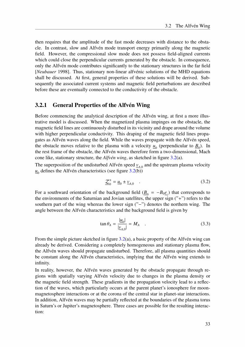
3.2 The Alfvén Wing
then requires that the amplitude of the fast mode decreases with distance to the obsta-cle. In contrast, slow and Alfvén mode transport energy primarily along the magneticfield. However, the compressional slow mode does not possess field-aligned currentswhich could close the perpendicular currents generated by the obstacle. In consequence,only the Alfvén mode contributes significantly to the stationary structures in the far field[Neubauer 1998]. Thus, stationary non-linear alfvénic solutions of the MHD equationsshall be discussed. At first, general properties of these solutions will be derived. Sub-sequently the associated current systems and magnetic field perturbations are describedbefore these are eventually connected to the conductivity of the obstacle.
3.2.1 General Properties of the Alfvén Wing
Before commencing the analytical description of the Alfvén wing, at first a more illus-trative model is discussed. When the magnetized plasma impinges on the obstacle, themagnetic field lines are continuously disturbed in its vicinity and drape around the volumewith higher perpendicular conductivity. This draping of the magnetic field lines propa-gates as Alfvén waves along the field. While the waves propagate with the Alfvén speed,the obstacle moves relative to the plasma with a velocity u0 (perpendicular to B0). Inthe rest frame of the obstacle, the Alfvén waves therefore form a two-dimensional, Machcone like, stationary structure, the Alfvén wing, as sketched in figure 3.2(a).The superposition of the undisturbed Alfvén speed vA,0 and the upstream plasma velocityu0 defines the Alfvén characteristics (see figure 3.2(b))
Z±
0= u0 ± vA,0 . (3.2)
For a southward orientation of the background field (B0 = −B0ez) that corresponds tothe environments of the Saturnian and Jovian satellites, the upper sign (”+”) refers to thesouthern part of the wing whereas the lower sign (”−”) denotes the northern wing. Theangle between the Alfvén characteristics and the background field is given by
tan θA =|u0|
|vA,0|= MA . (3.3)
From the simple picture sketched in figure 3.2(a), a basic property of the Alfvén wing canalready be derived. Considering a completely homogeneous and stationary plasma flow,the Alfvén waves should propagate undisturbed. Therefore, all plasma quantities shouldbe constant along the Alfvén characteristics, implying that the Alfvén wing extends toinfinity.In reality, however, the Alfvén waves generated by the obstacle propagate through re-gions with spatially varying Alfvén velocity due to changes in the plasma density orthe magnetic field strength. These gradients in the propagation velocity lead to a reflec-tion of the waves, which particularly occurs at the parent planet’s ionosphere for moon-magnetosphere interactions or at the corona of the central star in planet-star interactions.In addition, Alfvén waves may be partially reflected at the boundaries of the plasma torusin Saturn’s or Jupiter’s magnetosphere. Three cases are possible for the resulting interac-tion:
33
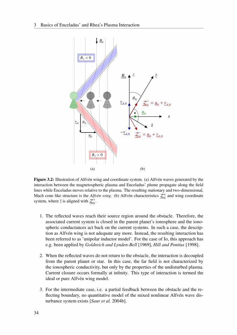
3 Basics of Enceladus’ and Rhea’s Plasma Interaction
Bx > 0
Bx < 0
B0
u0
θAvA
(a)
x
zzB0
Z+
0= u0 + vA,0
θA
u0
x
Z−
0= u0 + vA,0
−vA,0
vA,0
(b)
Figure 3.2: Illustration of Alfvén wing and coordinate system. (a) Alfvén waves generated by theinteraction between the magnetospheric plasma and Enceladus’ plume propagate along the fieldlines while Enceladus moves relative to the plasma. The resulting stationary and two-dimensional,Mach cone like structure is the Alfvén wing. (b) Alfvén characteristics Z±0 and wing coordinatesystem, where z is aligned withZ+
0 .
1. The reflected waves reach their source region around the obstacle. Therefore, theassociated current system is closed in the parent planet’s ionosphere and the iono-spheric conductances act back on the current systems. In such a case, the descrip-tion as Alfvén wing is not adequate any more. Instead, the resulting interaction hasbeen referred to as ’unipolar inductor model’. For the case of Io, this approach hase.g. been applied by Goldreich and Lynden-Bell [1969], Hill and Pontius [1998].
2. When the reflected waves do not return to the obstacle, the interaction is decoupledfrom the parent planet or star. In this case, the far field is not characterized bythe ionospheric conductivity, but only by the properties of the undisturbed plasma.Current closure occurs formally at infinity. This type of interaction is termed theideal or pure Alfvén wing model.
3. For the intermediate case, i.e. a partial feedback between the obstacle and the re-flecting boundary, no quantitative model of the mixed nonlinear Alfvén wave dis-turbance system exists [Saur et al. 2004b].
34
3.2 The Alfvén Wing
To check which of the models is the appropriate choice for the description of Enceladus’plasma interaction, the local plasma convection time τc has to be compared with theAlfvén travel time τA. The latter is defined as the time that is required for an Alfvénwave to travel from the moon to the parent planet’s ionosphere and back to the moonwhile τc is the time which is needed for a plasma element to cross the interaction region.If τA is large compared to τc, the interaction is not influenced by the planet’s ionosphereand the interaction is best described by the Alfvén wing model. For the average condi-tions at Enceladus, Saur et al. [2007] calculated τA ∼ 300 − 400 s and τc ∼ 10 s. Thus,τA τc is well fulfilled at Enceladus and the Alfvén wing model is suitable to describethe plasma interaction of Enceladus. A detailed study of the reflections of Enceladus’Alfvén wings at Saturn’s ionosphere (which do nevertheless occur) can be found in thework of Jacobsen [2011].Although, the work presented in this thesis focuses on Enceladus’ local interaction, i.e.the region within a few RE around the moon, effects of the far field interaction, whichinclude Saturn and the magnetosphere, shall be briefly discussed. The most prominentfar field effect is the generation of an auroral footprint of the Alfvén wing in Saturn’sionosphere by acceleration and precipitation of electrons into the ionosphere. The UV,IR and radio emissions of the footprint therefore indicate where the Alfvén wing reachesthe ionosphere (see, e.g. Clarke et al. [2004] for a discussion of Io’s footprint in Jupiter’sionosphere). Io’s primary footprint (leading spot) as well as multiple footprints of thereflected Alfvén wings have even been observed remotely by the HST [Bonfond et al.2008, 2009]. Enceladus’ footprint is unlikely more difficult to observe than that of Iodue the significantly lower energy flux towards the ionosphere: Enceladus’ interactiongenerates about 108 W, compared to a power of ∼ 1012 W in the Io scenario (values aretheoretical Poynting fluxes calculated by Saur et al. [2013]; the observable power is eventwo orders of magnitude lower). In agreement with that, Pryor et al. [2011] reported onthe detection of the Enceladus’ footprint by UVIS in 3 out of 313 images which were inprinciple favorable for the detection of the footprint. More recent data increased thesenumbers to 6 detections out of 316 images [Gurnett and Pryor 2012]. Interestingly, thesize of the footprint is considerably larger than the moon’s diameter, indicating that thesource region extends as far as 20RE. The brightness of the footprint varies even when it isvisible by a factor of about three, suggesting a strong variability in the plume source rate.Since the images of the footprint were obtained on 26 August 2008 (about two weeks afterthe E4 flyby), the plume was probably particularly active at that time. Pryor et al. [2011]also report on the detection of field-aligned ion and electron beams by CAPS, whichare likely associated with the reflection of the Alfvén wing. As discussed by Jacobsen[2011], the magnetometer observations obtained inbound of the E4 flyby show wave-likefield perturbations that seem to be related to these particle beams of the reflected wing.However, it remains puzzling why the E4 flyby was the only encounter that exhibited sucha signature.
35
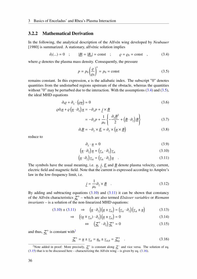
3 Basics of Enceladus’ and Rhea’s Plasma Interaction
3.2.2 Mathematical Derivation
In the following, the analytical description of the Alfvén wing developed by Neubauer[1980] is summarized. A stationary, alfvénic solution implies
∂t(...) = 0 ; |B| = |B0| = const ; % = %0 = const , (3.4)
where % denotes the plasma mass density. Consequently, the pressure
p = p0
(%
%0
)κ= p0 = const (3.5)
remains constant. In this expression, κ is the adiabatic index. The subscript ”0” denotesquantities from the undisturbed regions upstream of the obstacle, whereas the quantitieswithout ”0” may be perturbed due to the interaction. With the assumptions (3.4) and (3.5),the ideal MHD equations
∂t% + ∂x ·(%u
)= 0 (3.6)
%∂tu + %(u · ∂x
)u = −∂x p + j × B
= −∂x p +1µ0
−∂xB2
2+
(B · ∂x
)B
(3.7)
∂tB = −∂x × E = ∂x ×(u × B
)(3.8)
reduce to
∂x · u = 0 (3.9)(u · ∂x
)u =
(vA · ∂x
)vA (3.10)(
u · ∂x
)vA =
(vA · ∂x
)u . (3.11)
The symbols have the usual meaning, i.e. u, j, E and B denote plasma velocity, current,electric field and magnetic field. Note that the current is expressed according to Ampère’slaw in the low-frequency limit, i.e.
j =1µ0∂x × B . (3.12)
By adding and subtracting equations (3.10) and (3.11) it can be shown that constancyof the Alfvén characteristics Z± – which are also termed Elsässer variables or Riemanninvariants – is a solution of the non-linearized MHD equations:
(3.10) ± (3.11) ⇒(u · ∂x
) (u ± vA
)=
(vA · ∂x
) (vA ± u
)(3.13)
⇒((u ∓ vA) · ∂x
) (u ± vA
)= 0 (3.14)
⇔(Z∓· ∂x
)Z± = 0 (3.15)
and thus,Z± is constant with2
Z± = u ± vA = u0 ± vA,0 = Z±
0. (3.16)
2Note added in proof: More precisely, Z+ is constant along Z− and vice versa. The solution of eq.(3.15) that is to be discussed here – characterizing the Alfvén wing – is given by eq. (3.16).
36
3.2 The Alfvén Wing
With respect to the following calculations, it may also be useful to provide the magnitudeofZ±,
|Z±| = |u0 ± vA,0| =
√u2
0 + v2A,0 ± 2u0vA,0 cos
(]u0, vA,0
)(3.17)
= vA,0
√1 + M2
A . (3.18)
It is now helpful to apply a coordinate system x = (x, y, z), where the positive z-axis isaligned with the characteristics. Without loss of generality, z shall be aligned with Z+.The x-axis is perpendicular to z and located in the plane defined by the background mag-netic field B0 and the plasma flow u0. y is perpendicular to both, x and z. The orientationof y is chosen such that the coordinate system is right-handed. See also figure 3.2(b) foran illustration of this Alfvén wing coordinate system. Since the coordinate system whichis mainly used in this work is the interaction system of the respective satellite (ENISor RHIS), the physical quantities then need to be transformed from the wing coordinatesystem (x, y, z) to the interaction coordinate system (x, y, z). This transformation is givenby
x =1√
1 + M2A
(±x − MAz) (3.19)
y = y (3.20)
z =1√
1 + M2A
(MAx ± z) , (3.21)
with the upper sign denoting the northern wing and the lower sign referring to the southernwing.In the Alfvén wing coordinate system, writing equation (3.16) separately for the threecomponents and considering only the upper sign yields
ux + vA,x = 0 (3.22)uy + vA,y = 0 (3.23)uz + vA,z = const . (3.24)
It follows then that∂
∂zua = −
∂
∂zvA,a , (3.25)
where the subscript ’a’ denotes the components in the Alfvén wing coordinate system,a ∈ x, y, z. Inserting equations (3.22) – (3.24) and (3.25) in (3.14) (lower sign) yields[(
uz + vA,z)∂z
] (ua − vA,a
)= 0 (3.26)(
uz + vA,z) (∂zua − ∂zvA,a
)= 0 (3.27)
2(uz + vA,z
)(∂zua) = 0 , (3.28)
and therefore,∂
∂zu = 0 . (3.29)
37
3 Basics of Enceladus’ and Rhea’s Plasma Interaction
In a similar manner it can be shown that∂
∂zB = 0 . (3.30)
The same conclusion can be achieved, if z is aligned with the southern characteristicZ−. Therefore, velocity, magnetic field, electric field and current are constant along the
characteristics of the Alfvén wing.For a discussion of the current loops, the current is divided into a part j
⊥perpendicular to
Z+ and a part j
‖= j‖ ez = jz ez along the wing. Taking the divergence yields
∂x · j = ∂x · j⊥
+ ∂x · j‖
= ∂x · j⊥
+ ∂z jz = ∂x · j⊥
= 0 . (3.31)
The interpretation of equation (3.31) is that the perpendicular currents form closed currentloops, independent of the parallel currents. From Ampere’s law, the currents perpendicu-lar to the wing can be expressed as (equation (13) of Neubauer [1980])
j⊥
(x, y) = ( jx, jy, 0) =1µ0
(∂yBz,−∂xBz, 0) =1µ0
(∂xBz × ez
). (3.32)
To derive the parallel current, the divergence of the electric field is taken. Constancy ofZ
+ implies ∂x ×Z+ = 0 and thus,
∂x · E = ∂x ·(−u × B
)= ∂x ·
[−
(Z
+−
B√µ0ρ
)× B
]= Z+
· µ0 j = µ0vA
√1 + M2
A jz . (3.33)
Therefore, the current along the Alfvén characteristics can be expressed as
jz = ΣA∂x · E = −ΣA∂2xψ , (3.34)
with the electric potential ψ and the Alfvén conductance
ΣA =1
µ0vA
√1 + M2
A
. (3.35)
This conductance can be interpreted as a conductor situated perpendicular to the Alfvéncharacteristics with a uniform height-integrated conductivity ΣA [Neubauer 1980, 1998,Goertz 1980].The magnetic field perturbations perpendicular to the wing (B
⊥) can be derived from the
electric field according to
ez × E = ez × (−u × B)
= ez ×
(−(Z+
∓B√µ0ρ
) × B)
= +(ez · Z+)B − (ez · B)Z+
= vA
√1 + M2
AB − Bz vA
√1 + M2
Aez
= vA
√1 + M2
A B⊥
. (3.36)
38
3.2 The Alfvén Wing
Finally, we find for the magnetic field of the Alfvén wing (see Neubauer [1980])
B⊥
= (Bx, By, 0) =(ez × E
)µ0ΣA . (3.37)
The parallel field component is obtained by considering the constancy of B,
B‖
= (0, 0, Bz) = ±
√B2
0 − B2⊥ . (3.38)
Instead of the electric field, it is sometimes more convenient to consider the electric po-tential ψ. Faraday’s law and ∂z (...) = 0 imply Ez(x, y, z) to be constant. At large distancesto the wing, i.e.
√x2 + y2 → ∞, the electric field should be identical to the unperturbed
field E0 = −u0 × B0 = −E0 ey = −E0 ey. Therefore, it is Ez = 0 and the electric field canbe written as
E = −∂xψ = (−∂xψ,−∂yψ, 0) = (E x, Ey, 0) . (3.39)
In ENIS (or RHIS) coordinates, the magnetic field components(Bx, By, Bz
)associated
with the Alfvén wing can eventually be expressed as (see also Simon et al. [2011b] with∂zψ = 0)
Bx =1√
M2A + 1
∓MAΓ ± µ0ΣA
∂ψ
∂y
; (3.40)
By =1√
M2A + 1
µ0ΣA
∓∂ψ
∂x+ MA
∂ψ
∂z
; (3.41)
Bz =1√
M2A + 1
−Γ − MAµ0ΣA
∂ψ
∂y
, (3.42)
with
Γ =
√√B2
0 − µ20Σ
2A
1M2
A + 1
(±∂ψ
∂x− MA
∂ψ
∂z
)2
+
(∂ψ
∂y
)2 . (3.43)
At large distances to the wing – i.e.,√
x2 + y2 → ∞ – the Bx and the By perturbationsdecrease to zero, whereas Bz → −B0. Note that although the z component of the electricfield vanishes in the wing coordinate system (∂zψ = 0), this does not necessarily imply∂zψ = 0 in the interaction coordinate system.In the case of Enceladus, these expressions could be further simplified, since the mag-netic field perturbations in the far field do not depend on z for two reasons: The electroncollision frequency is clearly below the electron cyclotron frequency (νe Ωe), andtherefore the conductivity parallel to the magnetic field is large compared to the perpen-dicular conductivity. In consequence, the parallel electric field can be considered negligi-ble [Neubauer 1998]. For the low Alfvénic Mach number at Enceladus (MA ≈ 0.1) andcorresponding small angle θA < 10, it is also clear that z approximately coincides with z.Thus, at Enceladus electric field and electric potential do not depend on z, i.e. ∂zψ = 0.It should be pointed out that this analytical description of the Alfvén wing is based on theideal MHD equations without source or collision terms arising from the obstacle. Thus,
39
3 Basics of Enceladus’ and Rhea’s Plasma Interaction
the solution discussed above is valid only in the far field, i.e. sufficiently far away fromthe obstacle. Furthermore, this general solution does not explicitly include the propertiesof the obstacle, although its size and conductivity determine the electric potential ψ aswill be shown in the following sections.
3.2.3 Pedersen and Hall Currents
The coupling between the far field Alfvén wing solution and the conducting obstacle isprovided by the closure of the perpendicular currents arising from the interaction of theplasma flow with the obstacle.Therefore, a derivation of the perpendicular current after Neubauer [1998] and Simonet al. [2011b] will be presented in the following. While previously the MHD approachwas used, it is now necessary to consider a multi-fluid approach. In addition, the generalconducting obstacle is now specified by a cloud of neutral gas which can be ionized and/orwhich leads to collisions between the neutrals and the charged plasma. For a plasma fluidα, the momentum equation then reads
nαmα
duαdt
= − ∂x pα + qαnα(E + uα × B)
−∑
n
nαmανα,n(uα − un) −∑
n
S α,nmα(uα − un) (3.44)
= − ∂x pα + qαnα(E + uα × B) −∑
n
nαmανα,n(uα − un) . (3.45)
The parameters mα and να,n are the mass and the ion-neutral collision frequency of eachspecies, respectively. The subscript ’n’ denotes possible different neutral species. In thelast step, the collision frequency να,n and the source term S α,n have been merged into theeffective collision frequency να,n according to (see e.g. Neubauer [1998])
να,n =S α,n
nα+ να,n . (3.46)
Now, four simplifying assumptions are made: first, the velocity of the neutrals shall besmall compared to the velocity of the plasma species (|un| |uα|). Thereby, the momen-tum equation simplifies to
nαmα
duαdt
= −∂x pα + qαnα(E + uα × B) − nαmαναuα , (3.47)
whereνα =
∑n
να,n . (3.48)
Second, the electric field and magnetic field shall be given by E = E0 = −E0ey = −u0B0eyand B = B0 = −B0ez, respectively. Third, the thermal pressure is assumed to be negligiblecompared to dynamic and magnetic pressure, in agreement with the very low plasma betaat Enceladus (cf. table 2.4). Fourth, the plasma flow shall be stationary, i.e. mαduα/dt = 0.Solving equation (3.47) for the bulk speed uα of each component then yields
40
3.2 The Alfvén Wing
uα =1B0
ναΩα
ν2α + Ω2
α
−Ω2α
ν2α + Ω2
α
0
Ω2α
ν2α + Ω2
α
ναΩα
ν2α + Ω2
α
0
0 0Ωα
να
· E0 , (3.49)
where Ωα denotes the gyrofrequency of species α that is negative for electrons and positivefor ions, in agreement with the notation used by Simon et al. [2011b].For an ion species j, the (effective) collisions therefore yield a drift motion according to
u j,x = u0
Ω2j
ν2j + Ω2
j
, (3.50)
u j,y = −u0ν jΩ j
ν2j + Ω2
j
. (3.51)
The direction of the drift is given by u j = u0Ω j√Ω2
j +ν2j
(cos φ,− sin φ, 0), where the angle φ
reads
tan φ =
∣∣∣∣∣∣u j,y
u j,x
∣∣∣∣∣∣ =ν j
Ω j. (3.52)
The associated current density
j =∑α
nαqαuα (3.53)
can be computed according to
j = σ · E = σPE + σHB × E
B+ σ‖
(E · B
) BB2 , (3.54)
where the conductivity tensor with Pedersen conductivity σP, Hall conductivity σH andparallel conductivity σ‖ is given by
σ =
σP σH 0−σH σP 0
0 0 σ‖
. (3.55)
The elements of the conductivity tensor can be expressed as
σP =∑α
nαq2α
mα
ναν2α + Ω2
α
=∑α
nαqαB0
ναΩα
ν2α + Ω2
α
; (3.56)
σH = −∑α
nαq2α
mα
Ωα
ν2α + Ω2
α
= −∑α
nαqαB0
Ω2α
ν2α + Ω2
α
; (3.57)
σ‖ =∑α
nαq2α
mανα. (3.58)
41
3 Basics of Enceladus’ and Rhea’s Plasma Interaction
Instead of including ionization and the resulting pick-up in the Pedersen conductivityby means of the effective collision frequency, it is also possible to introduce a separatepick-up conductivity (cf. Goertz [1980]). For the sake of completeness, the derivationof the pick-up conductivity is summarized below. Due to ionization, a certain numberof electrons (S e) and ions (S i) is produced per unit volume and time. In agreement with|un| |uα|, it is assumed that ions and electrons are generated at rest. After accelerationby the electromagnetic fields, their guiding centers are displaced by
yguid = rg,αqα|qα|
, (3.59)
where rg,α is the gyroradius of ions (α = i) and electrons (α = e), respectively. The currentresulting from pick-up can therefore be expressed as
j =∑α=i,e
S α rg,α eE|E|
= σpickE , (3.60)
with the pick-up conductivity
σpick =∑α=i,e
S α mα
B20
. (3.61)
If the effective collision frequency does not include collisions, i.e.
να =S α
nα, (3.62)
the Pedersen conductivity converges to the pick-up conductivity in the limit να Ωα:
σP =∑α=i,e
nα qαB0
ναΩα
ν2α + Ω2
α
→∑α=i,e
nα qαB0
ναΩα
=∑α=i,e
nα qαB0
S α/nαΩα
=∑α=i,e
S α mα
B20
= σpick
(3.63)
and the Hall conductivity becomes zero.
Please note that additional contributions to the currents may not be caused by collisionsor pick-up but for example pressure gradients which were neglected above. However, itis not possible to assign a conductivity to e.g. the diamagnetic current caused by pressuregradients, because this current is not proportional to the electric field.
3.2.4 Potential Equation
In the following, the perpendicular current arising from the interaction of the neutral at-mosphere with the flow of magnetized plasma (equation (3.54)) will be connected to theAlfvén wing. For this calculation, the interaction coordinate system (x, y, z) will stillbe used and it is assumed that ∂zψ = 0 (see last paragraph of section 3.2.2). Initially,these calculations were carried out by Wolf-Gladrow et al. [1987] and Neubauer [1998],
42
3.2 The Alfvén Wing
whereas the computation shown here follows the summary of Simon et al. [2011b].
Exactly like in equation (3.31), the divergence of the current is split up into a parallel anda perpendicular contribution,
∂x · j⊥
= −∂z · j‖ . (3.64)
Integrating this equation yields
j‖(zmax) − j‖(zmin) =
zmax∫z=zmin
∂x · j⊥
dz , (3.65)
where zmin and zmax denote the lower and upper boundary of the integration, respectively.Inserting the electric potential ψ into the perpendicular current arising from Pedersen andHall conductivity (equation (3.54)) gives
j⊥
= −
σP
∂ψ
∂x+ σH
∂ψ
∂y
ex −
σP
∂ψ
∂y− σH
∂ψ
∂x
ey (3.66)
and thus,
∂x · j⊥
= −
σP∂
2xψ +
(∂σP
∂x−∂σH
∂y
)∂ψ
∂x+
(∂σP
∂y+∂σH
∂x
)∂ψ
∂y
. (3.67)
Inserting this equation in eq. (3.65) and introducing the height-integrated conductivities
ΣP,H =
∫ zmax
zmin
σP,H(x, y, z) dz (3.68)
results in
j‖(zmax) − j‖(zmin) = ΣP∂2xψ +
(∂ΣP
∂x−∂ΣH
∂y
)∂ψ
∂x+
(∂ΣP
∂y+∂ΣH
∂x
)∂ψ
∂y. (3.69)
To specify the upper and lower boundaries of the integration as well as the parallel currentat these boundaries, two cases are considered:
(1) The neutral gas cloud envelops a solid obstacle like an icy satellite and the magneticfield lines intersect the satellite. Without loss of generality, the analysis is restrictedto the northern hemisphere. The lower boundary of the integration (zmin) can thenbe identified with the surface of the satellite (see figure 3.3). According to thediscussion in section 3.1, no current flows through the surface of the icy moon andtherefore, it is
j‖(zmin) = 0 . (3.70)
The upper boundary can formally be set to infinity, where the Alfvén wing modelallows to express the parallel current as (cf. equation (3.34))
j‖(zmax) = −ΣA∂2xψ . (3.71)
43
3 Basics of Enceladus’ and Rhea’s Plasma Interaction
In this case, the integral (3.68) sums up all conductivity north of the solid obstacle.Inserting equations (3.70) and (3.71) into (3.69) yields the final form of the potentialequation:
(ΣP + ΣA) ∂2xψ +
(∂ΣP
∂x−∂ΣH
∂y
)∂ψ
∂x+
(∂ΣP
∂y+∂ΣH
∂x
)∂ψ
∂y= 0 . (3.72)
The same result can be obtained for the southern hemisphere.
(2) As illustrated in figure 3.3, further upstream or downstream of the obstacle theintegration along z may not intersect the solid body. In that case, the lower boundaryhas to be set to zmin = −∞ and the parallel current at zmin is also given by thecorresponding Alfvén wing far field current,
j‖(zmin) = +ΣA∂2xψ . (3.73)
The potential equation is accordingly modified to
(ΣP + 2ΣA) ∂2xψ +
(∂ΣP
∂x−∂ΣH
∂y
)∂ψ
∂x+
(∂ΣP
∂y+∂ΣH
∂x
)∂ψ
∂y= 0 . (3.74)
However, the integral (3.68) now contains all conductivity above and below theequatorial plane. Note that equation (3.74) assumes the form of equation (3.72), ifthe conductivitiesσP andσH are symmetric with respect to z = 0 and the integrationis performed from z = 0 to z = zmax.
A more general form of the potential equation which also includes the unipolar inductormodel has been derived by Saur [2004] and Saur et al. [2007].
3.2.5 Solution of the Potential Equation
To analytically solve the potential equation (3.72), which is an elliptic partial differentialequation of second order with variable coefficients, the obstacle is assumed to possess acylindrical symmetry. In two-dimensional polar coordinates x = (r cosϕ, r sinϕ, 0), thepotential equation reads
1r∂
∂ϕ
[(ΣP + ΣA)
∂ψ
∂ϕ
]+∂
∂r
[r (ΣP + ΣA)
∂ψ
∂r
]+∂ΣH
∂r∂ψ
∂ϕ−∂ΣH
∂ϕ
∂ψ
∂r= 0 . (3.75)
The overall idea is now to approximate the obstacle by subdomains with constant con-ductances. Within each of these volumes, the potential equation reduces to the two-dimensional Laplace equation
∂2xψ(x, y) = 0 , (3.76)
the general solution of which is given by
ψ(r, ϕ) =
∞∑k=1
rk(ak cos kϕ + bk sin kϕ) + r−k(gk cos kϕ + hk cos kϕ)
. (3.77)
44
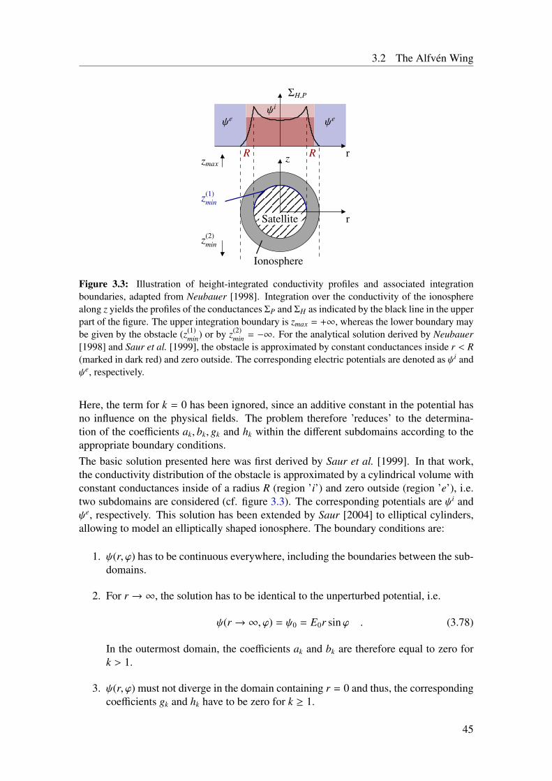
3.2 The Alfvén Wing
rz
r
zmax
z(1)min
z(2)min
R R
Ionosphere
ΣH,P
ψeψeψi
Satellite
Figure 3.3: Illustration of height-integrated conductivity profiles and associated integrationboundaries, adapted from Neubauer [1998]. Integration over the conductivity of the ionospherealong z yields the profiles of the conductances ΣP and ΣH as indicated by the black line in the upperpart of the figure. The upper integration boundary is zmax = +∞, whereas the lower boundary maybe given by the obstacle (z(1)
min) or by z(2)min = −∞. For the analytical solution derived by Neubauer
[1998] and Saur et al. [1999], the obstacle is approximated by constant conductances inside r < R(marked in dark red) and zero outside. The corresponding electric potentials are denoted as ψi andψe, respectively.
Here, the term for k = 0 has been ignored, since an additive constant in the potential hasno influence on the physical fields. The problem therefore ’reduces’ to the determina-tion of the coefficients ak, bk, gk and hk within the different subdomains according to theappropriate boundary conditions.The basic solution presented here was first derived by Saur et al. [1999]. In that work,the conductivity distribution of the obstacle is approximated by a cylindrical volume withconstant conductances inside of a radius R (region ’i’) and zero outside (region ’e’), i.e.two subdomains are considered (cf. figure 3.3). The corresponding potentials are ψi andψe, respectively. This solution has been extended by Saur [2004] to elliptical cylinders,allowing to model an elliptically shaped ionosphere. The boundary conditions are:
1. ψ(r, ϕ) has to be continuous everywhere, including the boundaries between the sub-domains.
2. For r → ∞, the solution has to be identical to the unperturbed potential, i.e.
ψ(r → ∞, ϕ) = ψ0 = E0r sinϕ . (3.78)
In the outermost domain, the coefficients ak and bk are therefore equal to zero fork > 1.
3. ψ(r, ϕ) must not diverge in the domain containing r = 0 and thus, the correspondingcoefficients gk and hk have to be zero for k ≥ 1.
45
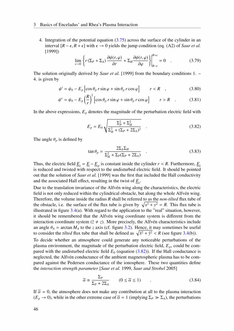
3 Basics of Enceladus’ and Rhea’s Plasma Interaction
4. Integration of the potential equation (3.75) across the surface of the cylinder in aninterval [R − ε,R + ε] with ε → 0 yields the jump condition (eq. (A2) of Saur et al.[1999])
limε→0
r (ΣP + ΣA)
∂ψ(r, ϕ)∂r
+ ΣH∂ψ(r, ϕ)∂ϕ
∣∣∣∣∣∣R+ε
R−ε
= 0 . (3.79)
The solution originally derived by Saur et al. [1999] from the boundary conditions 1. –4. is given by
ψi = ψ0 − Ep
[cos θp r sinϕ + sin θp r cosϕ
]r < R , (3.80)
ψe = ψ0 − Ep
(Rr
)2 [cos θp r sinϕ + sin θp r cosϕ
]r > R . (3.81)
In the above expressions, Ep denotes the magnitude of the perturbation electric field with
Ep = E0
√Σ2
P + Σ2H
Σ2H + (ΣP + 2ΣA)2
. (3.82)
The angle θp is defined by
tan θp =2ΣAΣH
Σ2H + ΣP(ΣP + 2ΣA)
. (3.83)
Thus, the electric field Ei = E − Ep is constant inside the cylinder r < R. Furthermore, Eiis reduced and twisted with respect to the undisturbed electric field. It should be pointedout that the solution of Saur et al. [1999] was the first that included the Hall conductivityand the associated Hall effect, resulting in the twist of Ei.Due to the translation invariance of the Alfvén wing along the characteristics, the electricfield is not only reduced within the cylindrical obstacle, but along the whole Alfvén wing.Therefore, the volume inside the radius R shall be referred to as the non-tilted flux tube ofthe obstacle, i.e. the surface of the flux tube is given by
√x2 + y2 = R. This flux tube is
illustrated in figure 3.4(a). With regard to the application to the ”real” situation, however,it should be remembered that the Alfvén wing coordinate system is different from theinteraction coordinate system (z , z). More precisely, the Alfvén characteristics includean angle θA = arctan MA to the z axis (cf. figure 3.2). Hence, it may sometimes be usefulto consider the tilted flux tube that shall be defined as
√x2 + y2 < R (see figure 3.4(b)).
To decide whether an atmosphere could generate any noticeable perturbations of theplasma environment, the magnitude of the perturbation electric field, Ep, could be com-pared with the undisturbed electric field E0 (equation (3.82)). If the Hall conductance isneglected, the Alfvén conductance of the ambient magnetospheric plasma has to be com-pared against the Pedersen conductance of the ionosphere. These two quantities definethe interaction strength parameter [Saur et al. 1999, Saur and Strobel 2005]
α ≡ΣP
ΣP + 2ΣA(0 ≤ α ≤ 1) . (3.84)
If α = 0, the atmosphere does not make any contribution at all to the plasma interaction(Ep → 0), while in the other extreme case of α = 1 (implying ΣP ΣA), the perturbations
46
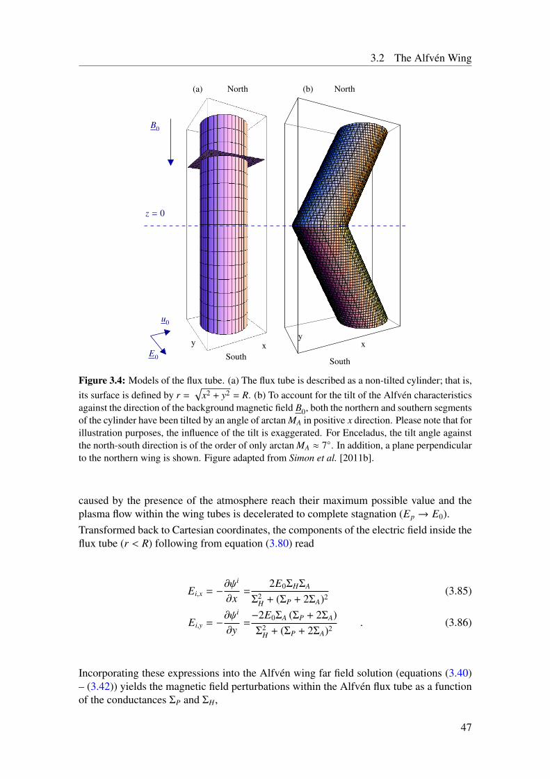
3.2 The Alfvén Wing
South
xy
North(a)
x
(b) North
y
South
u0
E0
z = 0
B0
Figure 3.4: Models of the flux tube. (a) The flux tube is described as a non-tilted cylinder; that is,its surface is defined by r =
√x2 + y2 = R. (b) To account for the tilt of the Alfvén characteristics
against the direction of the background magnetic field B0, both the northern and southern segmentsof the cylinder have been tilted by an angle of arctan MA in positive x direction. Please note that forillustration purposes, the influence of the tilt is exaggerated. For Enceladus, the tilt angle againstthe north-south direction is of the order of only arctan MA ≈ 7. In addition, a plane perpendicularto the northern wing is shown. Figure adapted from Simon et al. [2011b].
caused by the presence of the atmosphere reach their maximum possible value and theplasma flow within the wing tubes is decelerated to complete stagnation (Ep → E0).Transformed back to Cartesian coordinates, the components of the electric field inside theflux tube (r < R) following from equation (3.80) read
Ei,x = −∂ψi
∂x=
2E0ΣHΣA
Σ2H + (ΣP + 2ΣA)2
(3.85)
Ei,y = −∂ψi
∂y=−2E0ΣA (ΣP + 2ΣA)Σ2
H + (ΣP + 2ΣA)2. (3.86)
Incorporating these expressions into the Alfvén wing far field solution (equations (3.40)– (3.42)) yields the magnetic field perturbations within the Alfvén flux tube as a functionof the conductances ΣP and ΣH,
47
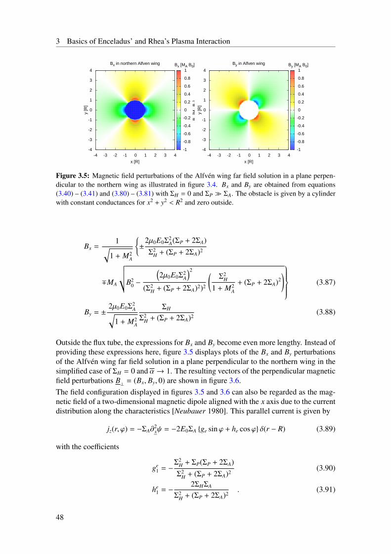
3 Basics of Enceladus’ and Rhea’s Plasma Interaction
Bx in northern Alfven wing Bx [MA B0]
-4 -3 -2 -1 0 1 2 3 4
x [R]
-4
-3
-2
-1
0
1
2
3
4
y [R
]
-1
-0.8
-0.6
-0.4
-0.2
0
0.2
0.4
0.6
0.8
1
Bx
[MA B
0]
By in Alfven wing By [MA B0]
-4 -3 -2 -1 0 1 2 3 4
x [R]
-4
-3
-2
-1
0
1
2
3
4
y [R
]
-1
-0.8
-0.6
-0.4
-0.2
0
0.2
0.4
0.6
0.8
1
Figure 3.5: Magnetic field perturbations of the Alfvén wing far field solution in a plane perpen-dicular to the northern wing as illustrated in figure 3.4. Bx and By are obtained from equations(3.40) – (3.41) and (3.80) – (3.81) with ΣH = 0 and ΣP ΣA. The obstacle is given by a cylinderwith constant conductances for x2 + y2 < R2 and zero outside.
Bx =1√
1 + M2A
±
2µ0E0Σ2A(ΣP + 2ΣA)
Σ2H + (ΣP + 2ΣA)2
∓MA
√√√B2
0 −
(2µ0E0Σ
2A
)2
(Σ2H + (ΣP + 2ΣA)2)2
(Σ2
H
1 + M2A
+ (ΣP + 2ΣA)2) (3.87)
By = ±2µ0E0Σ
2A√
1 + M2A
ΣH
Σ2H + (ΣP + 2ΣA)2
(3.88)
Outside the flux tube, the expressions for Bx and By become even more lengthy. Instead ofproviding these expressions here, figure 3.5 displays plots of the Bx and By perturbationsof the Alfvén wing far field solution in a plane perpendicular to the northern wing in thesimplified case of ΣH = 0 and α→ 1. The resulting vectors of the perpendicular magneticfield perturbations B
⊥= (Bx, By, 0) are shown in figure 3.6.
The field configuration displayed in figures 3.5 and 3.6 can also be regarded as the mag-netic field of a two-dimensional magnetic dipole aligned with the x axis due to the currentdistribution along the characteristics [Neubauer 1980]. This parallel current is given by
jz(r, ϕ) = −ΣA∂2xψ = −2E0ΣA ge sinϕ + he cosϕ δ(r − R) (3.89)
with the coefficients
ge1 = −
Σ2H + ΣP(ΣP + 2ΣA)Σ2
H + (ΣP + 2ΣA)2(3.90)
he1 = −
2ΣHΣA
Σ2H + (ΣP + 2ΣA)2
. (3.91)
48
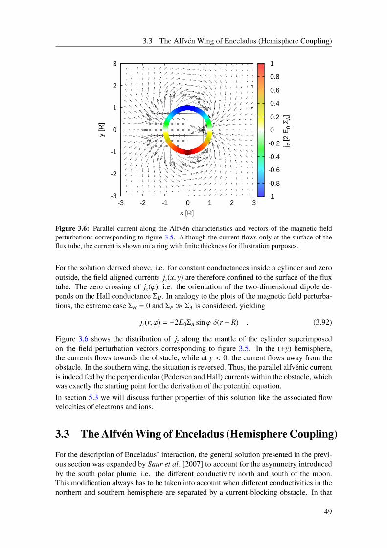
3.3 The Alfvén Wing of Enceladus (Hemisphere Coupling)
-3
-2
-1
0
1
2
3
-3 -2 -1 0 1 2 3
y [R
]
x [R]
-1
-0.8
-0.6
-0.4
-0.2
0
0.2
0.4
0.6
0.8
1
j z [2
E0
Σ A]
Figure 3.6: Parallel current along the Alfvén characteristics and vectors of the magnetic fieldperturbations corresponding to figure 3.5. Although the current flows only at the surface of theflux tube, the current is shown on a ring with finite thickness for illustration purposes.
For the solution derived above, i.e. for constant conductances inside a cylinder and zerooutside, the field-aligned currents jz(x, y) are therefore confined to the surface of the fluxtube. The zero crossing of jz(ϕ), i.e. the orientation of the two-dimensional dipole de-pends on the Hall conductance ΣH. In analogy to the plots of the magnetic field perturba-tions, the extreme case ΣH = 0 and ΣP ΣA is considered, yielding
jz(r, ϕ) = −2E0ΣA sinϕ δ(r − R) . (3.92)
Figure 3.6 shows the distribution of jz along the mantle of the cylinder superimposedon the field perturbation vectors corresponding to figure 3.5. In the (+y) hemisphere,the currents flows towards the obstacle, while at y < 0, the current flows away from theobstacle. In the southern wing, the situation is reversed. Thus, the parallel alfvénic currentis indeed fed by the perpendicular (Pedersen and Hall) currents within the obstacle, whichwas exactly the starting point for the derivation of the potential equation.In section 5.3 we will discuss further properties of this solution like the associated flowvelocities of electrons and ions.
3.3 The Alfvén Wing of Enceladus (Hemisphere Coupling)
For the description of Enceladus’ interaction, the general solution presented in the previ-ous section was expanded by Saur et al. [2007] to account for the asymmetry introducedby the south polar plume, i.e. the different conductivity north and south of the moon.This modification always has to be taken into account when different conductivities in thenorthern and southern hemisphere are separated by a current-blocking obstacle. In that
49
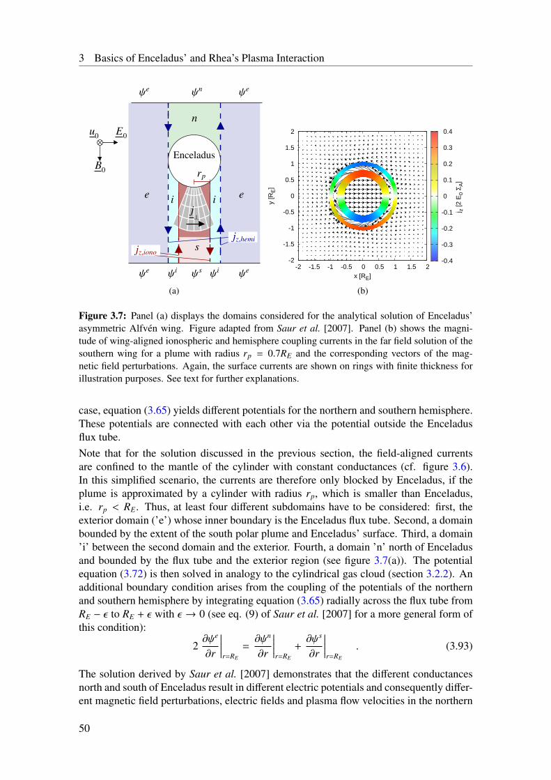
3 Basics of Enceladus’ and Rhea’s Plasma Interaction
u0
B0
E0
ψe
ψiψe ψiψs ψe
ψn ψe
e ei
s
n
i
Enceladus
rp
j⊥
jz,iono
jz,hemi
(a)
-2
-1.5
-1
-0.5
0
0.5
1
1.5
2
-2 -1.5 -1 -0.5 0 0.5 1 1.5 2y
[RE]
x [RE]
-0.4
-0.3
-0.2
-0.1
0
0.1
0.2
0.3
0.4
j z [2
E0
Σ A]
(b)
Figure 3.7: Panel (a) displays the domains considered for the analytical solution of Enceladus’asymmetric Alfvén wing. Figure adapted from Saur et al. [2007]. Panel (b) shows the magni-tude of wing-aligned ionospheric and hemisphere coupling currents in the far field solution of thesouthern wing for a plume with radius rp = 0.7RE and the corresponding vectors of the mag-netic field perturbations. Again, the surface currents are shown on rings with finite thickness forillustration purposes. See text for further explanations.
case, equation (3.65) yields different potentials for the northern and southern hemisphere.These potentials are connected with each other via the potential outside the Enceladusflux tube.Note that for the solution discussed in the previous section, the field-aligned currentsare confined to the mantle of the cylinder with constant conductances (cf. figure 3.6).In this simplified scenario, the currents are therefore only blocked by Enceladus, if theplume is approximated by a cylinder with radius rp, which is smaller than Enceladus,i.e. rp < RE. Thus, at least four different subdomains have to be considered: first, theexterior domain (’e’) whose inner boundary is the Enceladus flux tube. Second, a domainbounded by the extent of the south polar plume and Enceladus’ surface. Third, a domain’i’ between the second domain and the exterior. Fourth, a domain ’n’ north of Enceladusand bounded by the flux tube and the exterior region (see figure 3.7(a)). The potentialequation (3.72) is then solved in analogy to the cylindrical gas cloud (section 3.2.2). Anadditional boundary condition arises from the coupling of the potentials of the northernand southern hemisphere by integrating equation (3.65) radially across the flux tube fromRE − ε to RE + ε with ε → 0 (see eq. (9) of Saur et al. [2007] for a more general form ofthis condition):
2∂ψe
∂r
∣∣∣∣∣r=RE
=∂ψn
∂r
∣∣∣∣∣r=RE
+∂ψs
∂r
∣∣∣∣∣r=RE
. (3.93)
The solution derived by Saur et al. [2007] demonstrates that the different conductancesnorth and south of Enceladus result in different electric potentials and consequently differ-ent magnetic field perturbations, electric fields and plasma flow velocities in the northern
50
3.4 Enceladus’ Plasma Interaction: Measurements and Further Studies
and southern hemisphere. This implies that although northern and southern potential arenot directly linked, the northern potential is nevertheless affected by the southern plume.The coupling between the two hemispheres creates an additional surface current systemwhich is tangential to the Enceladus flux tube,
jz,hemisphere(r, ϕ) = 2E0ΣA ge sinϕ + he cosϕ δ(r − RE) . (3.94)
The wing-aligned current flowing at the surface of the ’plume-cylinder’, i.e. x2 + y2 = r2p
can be expressed as
jz,iono(r, ϕ) =4E0ΣAR2
E
r2p
gi sinϕ + hi cosϕ δ(r − rp) , (3.95)
where the coefficients are given by eqs. (17) – (23) of Saur et al. [2007]. Similar tofigure 3.7, both currents are displayed in figure 3.7(b) for ΣH = 0, ΣP ΣA and rp =
0.7RE. According to this analytical solution, the hemisphere coupling current systemshould always be present, if the Alfvénic, wing-aligned currents are (partially) blockedat the moon’s surface. As sketched in figure 1 of Saur et al. [2007], this even includesthe case in which the plume’s diameter is larger than the flux tube but the conductivity islargest below the south pole.To account for the finite conductivity in the outer regions of the plume, Simon et al.[2011b] further extended the solution of Saur et al. [2007] by considering even moresubdomains. These authors showed that their results are in good agreement with CassiniMAG data from several Enceladus flybys.It should be pointed out that the field-aligned currents on the mantle of the conduct-ing cylinder are surface currents due to the model assumption of constant conductanceswithin this cylinder. These currents generate a magnetic field discontinuity at the surfaceof the plume flux tube (see figure 3.5). However, if the conductances were not constant,these currents would be distributed over the whole cross-section of the cylinder and nodiscontinuity would occur. In contrast, the hemisphere coupling currents are always truesurface currents, regardless of the model assumptions. These currents therefore producereal and observable magnetic field discontinuities across the northern and southern Ence-ladus flux tube. At the time of the study of Saur et al. [2007], the Cassini spacecraft hadnot crossed this boundary, but as was shown by Simon et al. [2011b], these discontinuitiesindeed seem to be present at Enceladus (see also chapters 5 and 6).
3.4 Enceladus’ Plasma Interaction: Measurements andFurther Studies
After these theoretical descriptions of the plasma structures in Enceladus’ environment,the basic insights resulting from Cassini observations – apart from the findings of thisthesis – will be summarized. Note that this section focuses on the plasma structures,while the different models will be discussed in section 4.6.The first in-situ observations of plasma structures generated by the plume were alreadymade during the E0 and E1 flybys in February and March 2005 by the Cassini Mag-netometer [Dougherty et al. 2006]. The observed magnetic field signatures indicated a
51
3 Basics of Enceladus’ and Rhea’s Plasma Interaction
draping of the field lines around an ionospheric obstacle south of Enceladus, consistentwith the formation of an Alfvén wing. The magnetic field structures also suggested a slowdown of the plasma within the plume. The picture of an Alfvénic interaction could be fur-ther confirmed during the subsequent E2 encounter. Moreover, the observed signaturesexhibited the expected magnetic field pile-up upstream of the plume.During the E2 flyby, CAPS observed strong deflections in the plasma flow at least 27RE
away from Enceladus. Close to Enceladus, the plasma was found to be strongly sloweddown [Tokar et al. 2006]. It was concluded that the data are consistent with charge ex-change between the magnetospheric ions and the neutrals in Enceladus’ plume and thesubsequent pick-up of these newly generated ions. Although photo- and impact ionizationof neutrals could in principle lead to the same structures, RPWS did not detect a signif-icant increase of the plasma density during E2 (& 20%) and therefore, charge exchangewas suggested to be the dominant process for the plasma slow down and the deflections[Tokar et al. 2006]. By applying a steady-state model of the electrodynamic couplingbetween Enceladus and Saturn based on the unipolar inductor, Tokar et al. [2006] andPontius and Hill [2006] found that the amount charge exchange required to generate theobserved flow deflections corresponds to a total mass loading rate of more than 100 kg/s.As more flybys became available, CAPS detected freshly-produced water group ions (O+,OH+, H2O+, H3O+) close to Enceladus [Tokar et al. 2009]. Within the plume, the CAPSram anodes measured ions at energies corresponding to Cassini’s flyby velocity, whichimplies a (nearly) stagnating plasma flow within the plume. It is noteworthy that the slowdown of the plasma was measured four to six RE north of Enceladus. The observations offlow perturbations north of Enceladus are consistent with Cassini approaching the north-ern Alfvén wing.INMS measurements during the E3 flyby showed that out of the water group ion species,H3O+ is predominant within the plume [Cravens et al. 2009]. Another study of the ion-neutral chemistry in the plume has been presented by Fleshman et al. [2010a], furtherconfirming the importance of H3O+. A more detailed discussion of this findings will bepresented in section 6.4.1.Burger et al. [2007] developed a 3D Monte-Carlo model of the neutral plume to simulta-neously explain INMS and UVIS data. By including a detailed model of charge exchangeand ionization, these authors calculated a mass loading rate of 2 − 3 kg/s, i.e. two ordersof magnitude smaller than the value obtained by Tokar et al. [2006]. Furthermore, Burgeret al. [2007] suggested a plasma slow down to about 10 km/s which is less than 50% ofthe corotation speed but still significantly more than a stagnant plasma flow.Khurana et al. [2007] modeled the magnetic field data collected during the E0 – E2 flybysin 2005 in order to quantify the strength of Enceladus’ plasma interaction. These authorsconcluded that the effective diameter of the plume as an obstacle to the plasma flow is atleast 6RE, and the draping center3 of the magnetic field lines is displaced by more than2RE south of Enceladus and downstream by at least 1RE. In contrast to Pontius and Hill[2006], Khurana et al. [2007] estimate the total mass loading within 5RE of Enceladus to
3Note that in the work of Khurana et al. [2007] and Jia et al. [2010b,c], the term ”momentum loadingcenter” is used. Because the center is derived from the draping of the magnetic field lines, this location ismore appropriately described as the ”draping center”, especially since the draping center does not necessar-ily coincide with the region of highest momentum loading.
52
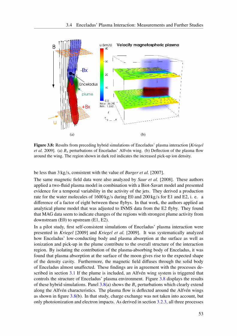
3.4 Enceladus’ Plasma Interaction: Measurements and Further Studies
(a) (b)
Figure 3.8: Results from preceding hybrid simulations of Enceladus’ plasma interaction [Kriegelet al. 2009]. (a) Bx perturbations of Enceladus’ Alfvén wing. (b) Deflection of the plasma flowaround the wing. The region shown in dark red indicates the increased pick-up ion density.
be less than 3 kg/s, consistent with the value of Burger et al. [2007].The same magnetic field data were also analyzed by Saur et al. [2008]. These authorsapplied a two-fluid plasma model in combination with a Biot-Savart model and presentedevidence for a temporal variability in the activity of the jets. They derived a productionrate for the water molecules of 1600 kg/s during E0 and 200 kg/s for E1 and E2, i. e. adifference of a factor of eight between these flybys. In that work, the authors applied ananalytical plume model that was adjusted to INMS data from the E2 flyby. They foundthat MAG data seem to indicate changes of the regions with strongest plume activity fromdownstream (E0) to upstream (E1, E2).In a pilot study, first self-consistent simulations of Enceladus’ plasma interaction werepresented in Kriegel [2009] and Kriegel et al. [2009]. It was systematically analyzedhow Enceladus’ low-conducting body and plasma absorption at the surface as well asionization and pick-up in the plume contribute to the overall structure of the interactionregion. By isolating the contribution of the plasma-absorbing body of Enceladus, it wasfound that plasma absorption at the surface of the moon gives rise to the expected shapeof the density cavity. Furthermore, the magnetic field diffuses through the solid bodyof Enceladus almost unaffected. These findings are in agreement with the processes de-scribed in section 3.1 If the plume is included, an Alfvén wing system is triggered thatcontrols the structure of Enceladus’ plasma environment. Figure 3.8 displays the resultsof these hybrid simulations. Panel 3.8(a) shows the Bx perturbations which clearly extendalong the Alfvén characteristics. The plasma flow is deflected around the Alfvén wingsas shown in figure 3.8(b). In that study, charge exchange was not taken into account, butonly photoionization and electron impacts. As derived in section 3.2.3, all three processes
53
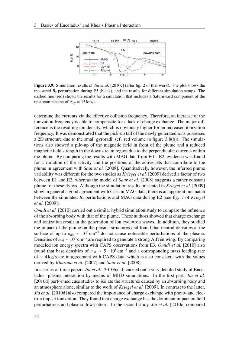
3 Basics of Enceladus’ and Rhea’s Plasma Interaction
Figure 3.9: Simulation results of Jia et al. [2010c] (after fig. 2 of that work). The plot shows themeasured By perturbation during E5 (black), and the results for different simulation setups. Thedashed line (red) shows the results for a simulation that includes a Saturnward component of theupstream plasma of u0,y = 15 km/s.
determine the currents via the effective collision frequency. Therefore, an increase of theionization frequency is able to compensate for a lack of charge exchange. The major dif-ference is the resulting ion density, which is obviously higher for an increased ionizationfrequency. It was demonstrated that the pick-up tail of the newly generated ions possessesa 2D structure due to the small gyroradii (cf. red volume in figure 3.8(b)). The simula-tions also showed a pile-up of the magnetic field in front of the plume and a reducedmagnetic field strength in the downstream region due to the perpendicular currents withinthe plume. By comparing the results with MAG data from E0 – E2, evidence was foundfor a variation of the activity and the positions of the active jets that contribute to theplume in agreement with Saur et al. [2008]. Quantitatively, however, the inferred plumevariability was different for the two studies as Kriegel et al. [2009] derived a factor of twobetween E1 and E2, whereas the model of Saur et al. [2008] suggests a rather constantplume for these flybys. Although the simulation results presented in Kriegel et al. [2009]show in general a good agreement with Cassini MAG data, there is an apparent mismatchbetween the simulated By perturbations and MAG data during E2 (see fig. 7 of Kriegelet al. [2009]).Omidi et al. [2010] carried out a similar hybrid simulation study to compare the influenceof the absorbing body with that of the plume. These authors showed that charge exchangeand ionization result in the generation of ion cyclotron waves. In addition, they studiedthe impact of the plume on the plasma structures and found that neutral densities at thesurface of up to nn0 ∼ 106 cm−3 do not cause noticeable perturbations of the plasma.Densities of nn0 ∼ 108 cm−3 are required to generate a strong Alfvén wing. By comparingmodeled ion energy spectra with CAPS observations from E3, Omidi et al. [2010] alsofound that base densities of nn0 ∼ 5 · 108 cm−3 and a corresponding mass loading rateof ∼ 4 kg/s are in agreement with CAPS data, which is also consistent with the valuesderived by Khurana et al. [2007] and Saur et al. [2008].In a series of three papers Jia et al. [2010b,c,d] carried out a very detailed study of Ence-ladus’ plasma interaction by means of MHD simulations. In the first part, Jia et al.[2010d] performed case studies to isolate the structures caused by an absorbing body andan atmosphere alone, similar to the work of Kriegel et al. [2009]. In contrast to the latter,Jia et al. [2010d] also compared the importance of charge exchange with photo- and elec-tron impact ionization. They found that charge exchange has the dominant impact on fieldperturbations and plasma flow pattern. In the second study, Jia et al. [2010c] compared
54
3.4 Enceladus’ Plasma Interaction: Measurements and Further Studies
their results with MAG data from the E2 and E5 flybys to analyze the shape of the plume.They found that the magnetic field signatures agree best with a plume opening angle of10 − 20 and a tilt angle of 10 towards downstream which is also in agreement withKriegel et al. [2009]. Furthermore, their model suggests that mass loading in the plume isless efficient close to the surface of the moon, although the neutral density is highest nearthe surface. Their modeled ion densities show an increase of about 50% due to photo-and electron impact ionization. Currents arising from charge exchange, however, gen-erate over 90% of the strength of the field perturbations. Although their results were ingood agreement with the observed Bx and Bz components for both flybys, By was not re-produced by the simulations as shown in figure 3.9. This is similar to the results of Kriegelet al. [2009], who found a disagreement between simulated and measured By componentfor the E2 flyby (cf. fig. 7 in that work). Therefore, Jia et al. [2010c] suggested thatan upstream velocity component towards Saturn is required to explain the observed By
perturbations. Furthermore, Jia et al. [2010c] found that variations in the gas productionrate cause significant variations in the Bz perturbations, while variations in the upstreamdensity mainly modify the Bx and By perturbations. This finding is in agreement withthe theoretical point of view developed in the previous sections: On the one hand, the Bz
perturbation is not part of the Alfvén wing far field solution, but it is directly generated bythe perpendicular Pedersen and Hall currents in the plume. The strength of these currentstherefore increases with higher neutral densities. On the other hand, the Bx perturbationin the center of the Alfvén wing in the far field (equation (3.87)) can be approximatedas Bx ≈ αMAB0. For α → 1, the Bx perturbations depend only on the upstream density,Bx ∼
√n0. In their third study, Jia et al. [2010b] analyzed the variability of the plume by
considering the strength of the Bz perturbations. It was found that the maximum variationof the gas production rate is about 30% which is a clearly lower variability than the factorof eight between E0 and E1/E2 derived by Saur et al. [2008]. The plasma momentumloading rate ranges from 0.8 to 1.9 kg/s, which is consistent with previous studies. Themodel of Jia et al. [2010b] also required that the momentum loading rate per neutral den-sity is reduced close to the surface by orders of magnitude compared to larger distances.It it suggested that a depletion of hot electrons and a decrease in the charge exchange ratemay explain the reduction of the momentum loading rates close to the south pole.Another important finding has been made by analyzing data that has been collected by theRPWS Langmuir probe during the E2 encounter: the presence of a significant imbalancebetween the number densities of free electrons and ions, coinciding with an increase inthe density of submicron dust grains [Wahlund et al. 2009, Yaroshenko et al. 2009]. Thus,this void in the electron density is suggested to arise from electron absorption by dust. Inagreement with that, analysis of the upper hybrid frequency emissions recorded by RPWSduring E3 indicated an electron dropout to below ne = 20 cm−3 within the plume [Farrellet al. 2009]. The density of charged dust corresponding to the difference of electron andion densities observed by the Langmuir Probe during E3 has been used by Shafiq et al.[2011] to infer characteristics of the charged dust population. These authors concludedthat the Debye length of these charged dust grains is large compared to the average dis-tance between the grains and hence, the charged dust has to be taken into account as anadditional plasma constituent. Interpretation of Langmuir Probe data from the steep fly-bys E3 – E6 has also been performed by Morooka et al. [2011]. These authors suggestedenormous ion densities of 30, 000 − 100, 000 cm−3 due to ionization within the plume,
55
3 Basics of Enceladus’ and Rhea’s Plasma Interaction
whereas the suggested electron densities are in the range of 2, 000 − 4, 000 cm−3, therebyimplying that more than 90% of the electrons are absorbed by the dust. However, Mo-rooka et al. [2011] did not present any quantitative estimates with regard to the processesgenerating these extremely high densities.Apart from the indirect hints towards the presence of charged dust by the discrepancyof electron and ion densities, there is also direct evidence for charged nanograins inthe plume reported by the CAPS. Although originally designed for detecting electronsand ions in a wide energy range, the instrument detected high counting rates at energies> 1 keV when Cassini was traveling through the plume. These were interpreted as thesignatures of charged nanograins [Jones et al. 2009]. The nanograins were observed ascollimated jets and seem to be separated according to their charges and masses. Interest-ingly, both, positive and negative grains were observed. Further analysis of these data byCoates et al. [2010] indicated the presence of negative ions, i.e. negatively charged watergroup clusters with masses up to 72 amu. Hill et al. [2012] used CAPS data from E3and E5 to derive the densities of the nanograins. These authors suggested that the densityof the negative nanograins reached values of up to 2600 e/cm−3 during E3, whereas thedensity of the positive grains is about three orders of magnitude lower.In addition, RPWS recorded strong broadband whistler mode emissions, called auroralhiss [Gurnett et al. 2011]. It is suggested that the electrons generating the auroral hissare accelerated by parallel electric fields in a region very close to the moon. A surveyof the auroral hiss observations of all 20 flybys has been carried out by Leisner et al.[2013]. These authors found that all emissions are generated by field-aligned electronbeams either in the region upstream and Saturnward of Enceladus or downstream and atthe Saturn-averted side.More recently, Ozak et al. [2012] analyzed CAPS electron data from E5 by applyinga two-stream electron transport model. Their modeled electron fluxes agree well withCAPS data, thereby suggesting that photoelectrons with energies between 10 eV and70 eV are consistent with the data. Furthermore, Ozak et al. [2012] concluded that ionproduction due to electron impacts is only about 20% that of photoionization. However,the photoelectrons considered by Ozak et al. [2012] are mainly of magnetospheric origin.In constrat, Coates et al. [2013] showed that photoelectron locally produced within theplume had been detected by CAPS during nearly all Enceladus encounters. These authorssuggested that the plume photoelectrons increase the electron flux at energies of about 20eV by about a factor of two and thus, photoelectrons have to be taken into account as anadditional ionization source.
3.5 Summary of Enceladus’ Plasma Interaction and OpenQuestions
The plasma interaction of Enceladus features the unique situation in which an absorbingbody is placed above the plume as an ionosphere-type obstacle. Therefore, the resultinginteraction with the subalfvénic flow of magnetospheric plasma contains aspects of bothscenarios. Previous studies, however, indicate that the plasma structures generated by theplume dominate the overall interaction and the structures caused by plasma absorption
56
3.5 Summary of Enceladus’ Plasma Interaction and Open Questions
at the moon (see section 3.1) are less important at Enceladus [Kriegel et al. 2009, Jiaet al. 2010d]. Within the plume, the neutral molecules are mainly ionized due to chargeexchange and to a lesser extent by photoionization and electron impacts. The momentumand mass loading of a few kg/s of ions leads to a nearly stagnant plasma flow in the centerof the plume as observed by CAPS [Tokar et al. 2006]. Furthermore, ionization andion-neutral collisions result in the generation of Pedersen and Hall currents in the plume.These transverse currents cause a magnetic pile-up region at the ramside of the plumeand reduce the magnetic field strength in the downstream region. In the rest frame of theincident plasma, these currents are closed by the field-aligned currents of a stationary,non-linear system of Alfvén waves, the Alfvén wing. Transformed to the rest frame ofthe moon, the currents flow along the Alfvén characteristicsZ±, which are tilted towardsthe corotation direction by an angle of θA ≈ 5 − 10 with respect to the background field.In the far field (i.e. where the magnetic field generated by Pedersen and Hall currentscan be neglected), the wing current system exhibit translation symmetry along the wingcharacteristics (see e.g. Neubauer [1980, 1998], Saur et al. [1999] and references therein).The associated magnetic field perturbations have been detected by Cassini MAG duringall Enceladus encounters. Furthermore, Saur et al. [2007] proposed an additional currentsystem that arises from the partial blockage of the Alfvénic field-aligned currents by thesolid body of the moon. This current system connects Enceladus’ northern and southernhemispheres and therefore, it is referred to as ’hemisphere coupling currents’. Since thesecurrents are surface currents flowing on field lines tangential to Enceladus, they causediscontinuities in the magnetic field which have been observed by Cassini MAG.Overall, a broad and detailed understanding of Enceladus’ plasma interaction was alreadyavailable prior to this thesis. However, a comparison between Cassini MAG data andpreceding hybrid simulations [Kriegel et al. 2009] as well as MHD simulations by Jiaet al. [2010b,c] also revealed some apparent mismatches which seem to contradict thetheory depicted in this chapter. In addition, the presence of charged dust has not beentaken account by these studies. Thus, the following issues shall be addressed within thisthesis:
• Various measurements indicate that the negatively charged dust within the plumeexhibits densities comparable to the ion densities [Yaroshenko et al. 2009, Shafiqet al. 2011, Morooka et al. 2011, Hill et al. 2012]. Thus, the main topic of this thesisis to investigate what effects on the plasma structures are caused by the presence ofthe charged dust.
• What is the reason for the striking difference between modeled and measured By
perturbations? If the explanation was a radial flow component of the magneto-spheric plasma as suggested by Jia et al. [2010c], how does such a flow pattern fitin the understanding of Saturn’s magnetosphere (see section 2.2)? What other ex-planations are possible and how could they be integrated into the existing theoreticalframework? These questions will be addressed and answered in chapter 5.
• The models of Khurana et al. [2007] and Jia et al. [2010b,c] indicate that the drap-ing center is displaced from the surface to the south and downstream. Jia et al.[2010b] proposed that a reduction of the reaction and ionization rates may yieldthis shift of the draping center. It will therefore be analyzed in chapters 5 and 6,
57
3 Basics of Enceladus’ and Rhea’s Plasma Interaction
whether and under what assumptions, the hybrid simulations in combination withdata from the steep Enceladus flybys E3 – E6 can reproduce this location of thedraping center. In this sense, MAG data shall also be used as a sensitive probe tofurther constrain the structure and properties of the neutral plume.
• Between 2009 and 2014, 13 additional Enceladus flybys took place that had notbeen analyzed in the simulation studies of Jia et al. [2010b,c] and Kriegel et al.[2009]. Do the (magnetic field) data collected along these trajectories confirm ourunderstanding of Enceladus plasma interaction or do new questions arise? Withmore flybys available, the variability of the plume is also to be constrained in moredetail in chapter 5.
• Although charge exchange has the dominant impact on the plasma flow, photoion-ization and electron impacts are responsible for the increased ion density in theplume. In chapter 6, the combination of a detailed model of the reaction and ion-ization rates with a sophisticated model of the neutral plume shall allow to quanti-tatively determine the increase of the ion density.
58
4 Hybrid Simulation Code A.I.K.E.F.
In this chapter, the main features of the simulation model are described. After a briefoverview about the hybrid approach and the simulation code A.I.K.E.F., the unique as-pects of the modeling of Enceladus’ plasma interaction are discussed. In particular, theimplementation of collisions and reactions is discussed in some detail. Furthermore, theboundary conditions applied within the simulation model will be described and their in-fluence on the physical structures will be analyzed. Finally, an overview of the existingmodels of Enceladus’ plasma interaction is provided.
4.1 Hybrid Approach: Basic Assumptions and Equations
Since the hybrid model used in this work has already been described in detail in theliterature (e. g. Bagdonat and Motschmann [2002b], Simon [2007]), the assumptions andequations of the hybrid model will only be briefly reviewed. For a more general overviewabout hybrid models and their implementations, the reader is referred to Winske et al.[2003].The hybrid approach treats the electrons as a massless, charge-neutralizing fluid. Sincethe ions are represented by individual particles, the model can handle multiple ion speciesand does not require any assumptions on the velocity distribution of the ions. The ap-proximation of electrons as a fluid is well fulfilled if the time and spatial scales of theinvestigated processes are clearly larger than the electron gyration period and the electrongyration radius, respectively.
The hybrid model used in this thesis is based on three basic assumptions:
• The electron mass me is neglected,
me ≈ 0 . (4.1)
• The plasma is assumed to be quasi-neutral, i. e. for a plasma consisting of α =
1, ...,N species with densities nα and charges qα, it isN∑α=1
qαnα = 0 . (4.2)
Therefore, the length scales are assumed to be much larger than the Debye lengthλD, which assumes values of a few meters in the vicinity of Enceladus and sometens of meters near Rhea.
59
4 Hybrid Simulation Code A.I.K.E.F.
• The Darwin-Approximation [Bagdonat 2004] is used which means that the dis-placement current is neglected. Ampère’s law then reads
∂x × B = µ0 j . (4.3)
Thus, all velocities have to be well below the speed of light.
From these few assumptions, the basic equations of the model can be derived.To show how even a negatively charged ion or dust species can be included in the frame-work of the hybrid model, the general derivation of the equation for the electric field isreviewed. The electron momentum equation for zero electron mass and isotropic pressurereads
E = −ue × B −∂x pe
ene+ η j , (4.4)
where ue denotes the electron bulk speed and pe is the electron pressure. The last termdescribes the diffusion of the electromagnetic fields through a medium of finite resistivityη or corresponding conductivity σ = 1/η, which may arise from the moon’s solid body,see section 4.5.1. In addition, this resistivity mimics the effects of electron-ion collisionsor wave-particle scattering. Using the definition of the current j,
j =∑α
qαnαuα =∑
j
q jn ju j − eneue , (4.5)
and rearranging for the electron velocity ue yields
ue =
∑j
q jn ju j − j
ene=
∑j
q jn ju j − j∑j
q jn j, (4.6)
where uα/ j denotes the bulk velocity of species α/ j. In the last step, the quasi-neutralitycondition (4.2) has been used. It may be defined that here and in the following, thesubscript ’α’ runs over all plasma species (ions and electrons) while the subscript ’ j’ isonly used for the ion species.Inserting equations (4.2), (4.6) and (4.3) into (4.4) finally yields the equation for the elec-tric field in the hybrid model:
E = −
∑j
q jn ju j∑j
q jn j× B +
(∂x × B) × Bµ0
∑j
q jn j−
∂x pe∑j
q jn j+ η
∂x × Bµ0
. (A)
The substitution ∑j
q jn ju j∑j
q jn j= ui (4.7)
leads to the more common form of equation (A) that is usually given in the literature. Notethat in this general case, ui is the charge-averaged ion velocity, which is identical to the
60
4.1 Hybrid Approach: Basic Assumptions and Equations
number-density averaged velocity only in the simple case with singly-charged, positiveion species. Therefore, |ui| may become larger than each species’ bulk velocity |u j|, ifnegatively charged ion or dust species are involved.It should be noted that the denominators in equation (A) must not be zero. Thus, a mini-mum positive charge density ρmin is introduced. If the density at some point in the simu-lation box drops below that threshold, the denominators are set equal to ρmin to avoid thatthe field diverges. The value of the minimum charge density ρmin is set to ρmin = 0.1en∗0and ρmin = 0.15en∗0 for the simulations presented in chapter 5 and 6, respectively, whatcorresponds to 10 % (15 %) of the upstream ion density n∗0.When considering ρmin, the model is capable of handling a negatively charged ion or dustspecies without any modifications. In section 6.3, it will be shown that dust (subscript’D’) can be described as a heavy, negatively charged ion species. Assuming that the dustmay be charged with ξ electrons, i. e.
%D = −eξnD , (4.8)
it is ∑j
q jn j =∑
jq j>0
q jn j − eξnD > ρmin . (4.9)
In this hybrid model, the equation of state for the electrons is provided by an adiabaticlaw for the pressure:
pe =∑
j
pe, j =∑
j
pe, j0
(ne j
ne, j0
)κ. (B)
The quantities pe, j0 and ne, j0 denote pressure and density of the undisturbed upstreamplasma. The adiabatic exponent κ is set to κ = 2. This choice considers that the magneticfield reduces the degrees of freedom of the electrons to two (see e.g, Bagdonat [2004] andSimon [2007]). The subscript ′ j′ indicates that different electron populations are assignedto the respective ion species. This description takes into account that the temperature ofthe upstream electrons may be considerably different from that of the ionospheric elec-trons. The approach of different electron populations is a good approximation only inregions where these populations do not mix. Otherwise, this concept may lead to contra-dictory results, see Ranocha [2013]. However, it should be pointed out that due to the lowelectron plasma beta of only βe = 0.0004 at Enceladus (cf. table 2.4), the electron pres-sure has a negligible impact on the plasma structures. Apart from the adiabatic law, otherways to close the set of equations are also possible, for instance a study that included thetime evolution of the electron pressure in the hybrid model has recently been presentedby Ranocha [2013].Finally, the time evolution of the magnetic field can be obtained by applying Faraday’slaw to eq. (A),
61
4 Hybrid Simulation Code A.I.K.E.F.
∂tB = ∂x ×(ui × B
)− ∂x ×
∂x × (∂x × B)µ0
∑j
q jn j
− ∂x ×
(η
µ0∂x × B
). (C)
Note that due to the adiabatic law, the curl of the pressure term vanishes and this termdoes not appear in equation (C).Since the ions are treated as particles, they may be generated or lost by ionization, recom-bination, reactions or absorption at the satellite’s surface. The motion of an individualparticle ’p’ is governed by the Lorentz force according to
dxp, j
dt= vp, j ;
dvp, j
dt=
q j
m j
(E′ + vp, j × B
), (D)
where the modified electric field E′ = E − η j is required to conserve the total momentumof the system [Bagdonat 2004].
4.2 Numerical Implementation
The implementation of the hybrid model used in this work is the simulation code A.I.K.E.F.(Adaptive Ion-Kinetic Electron-Fluid) [Müller et al. 2011]. It is the successor of the”Braunschweig Code” which has been applied to the plasma interaction of various objectsin the solar system within the last decade. In particular, A.I.K.E.F. had already been usedfor the preceding study of Enceladus’ plasma interaction [Kriegel et al. 2009] whereasthe Braunschweig-Code had been applied for simulations of Rhea’s plasma interaction byRoussos et al. [2008a]. A detailed description of the numerical aspects of A.I.K.E.F. isgiven by Müller et al. [2011]. Therefore, just a short summary and some details whichare complementary to the aforementioned studies will be provided here.A.I.K.E.F. operates on Cartesian meshes, where the resolution can locally be increasedaccording to the structures of interest. The refinement is implemented as ”Hybrid BlockAdaptive Mesh Refinement” (AMR). The mesh is decomposed into equally sized blocks(L0-blocks). Each block is again divided into eight octants. If a certain criterion is ful-filled (either predefined or dynamically computed during simulation runtime), the octantbecomes a new block of the next higher level of refinement. The cell size of this newblock is therefore a factor of two smaller. This method allows a good adjustment of theregions of higher mesh resolution to the features of interest together with an efficient com-putation. Theoretically, an arbitrary number of refinement levels may be used. However,it turned out that calculations with more than four levels (L0, L1, L2, L3) take too long forour purposes. The code is parallelized via the Message Passing Interface (MPI) such thateach process is assigned a certain number of blocks. The number of blocks handled bya process is adjusted in the way that the workload of all processes is similar. For thesimulations performed for this thesis, the computation time speedup of A.I.K.E.F. scalesalmost linearly with the number of processors until at least 128 CPUs. Therefore, and dueto the available computational resources, nearly all simulations were carried out on 128
62
4.2 Numerical Implementation
CPUs.A.I.K.E.F. is a Particle-in-Cell code, which means that the macroscopic physical quan-tities are computed only at the mesh nodes of the simulation grid while the ions (whichare represented by macroparticles with the same charge-to-mass ratio as the real particles)can move freely within the cells. The contribution of a macroparticle to the macroscopicmoments at the mesh nodes of the respective cell as well as the electromagnetic fieldsat the particle’s position are inter-/extrapolated with the trilinear Cloud-in-Cell method.However, the different cells sizes of the mesh require some additional procedures for theparticles: when moving from a lower to s higher level of refinement, one cell is dividedinto eight smaller cells. In consequence, a certain number of macroparticles in the largercells (typically ∼ 100) would yield on average a factor of eight less macroparticles inthe smaller cells. When crossing even more levels, e.g. from L0 to L3, some cells ofL3 may be completely devoid of particles. The opposite effect occurs when starting withabout 100 macroparticles in the highest level and moving into larger cells. In this case, thenumber of macroparticles in the cells of L0 would be drastically enhanced, yielding a veryinefficient and slow computation. Therefore, the number of macroparticles in each cell isadjusted next to the refinement boundaries. On the one hand, this is done by splitting oneparticle into two if there are too few macroparticles in the respective cell. On the otherhand, three particles are merged into two if there are too many particles. Details on thesplitting and merging in A.I.K.E.F. can be found in Müller [2012].The electric field is advanced in time via the Current Advance Method [Matthews 1994].The convective term and the Hall term of the magnetic field equation,
∂tB = ∂x ×(ui × B
)− ∂x ×
∂x × (∂x × B)µ0
∑j
q jn j
= f (B) (4.10)
are advanced in time by means of a second-order cyclic leap-frog algorithm, which isexplicit in time (see section 4.3.1 of Bagdonat [2004] and references therein). The majordisadvantage of this algorithm is that the numerical solution may be artificially amplifiedcompared to the analytical solution which makes the simulation unstable. Therefore, anadditional smoothing procedure has to be performed (see section 4.4). The diffusion termof the magnetic field equation,
∂tB = −∂x ×
(η
µ0∂x × B
)= g(B) , (4.11)
is more difficult to numerically solve due to the sharp gradient of the resistivity η at thesurface of the moon (see section 4.5.1 for a discussion of the obstacles’ resistivity). If theleap-frog algorithm was applied to equation (4.11), a stable simulation would require asignificantly smaller time step and an associated longer simulation time. Thus, an implicitCrank-Nicolson algorithm
Bn+1 − Bn
∆t=
12
(g(Bn+1) + g(Bn)
)(4.12)
is applied to advance the diffusion term from time step n to time step n+1. This algorithmhas the advantage that the numerical amplification is always equal to one. To solve this
63
4 Hybrid Simulation Code A.I.K.E.F.
implicit equation, the iterative Successive-Over-Relaxation (SOR) scheme is used,
Bnew = (1 − ωS OR)Bold + ωS ORB∗ . (4.13)
Here, B∗ is a function of the coefficients and differential operators of equation (4.11). Theoverrelaxation parameterωS OR guarantees convergence for 1 < ωS OR < 2. The exact valueof ωS OR which enables the fastest convergence can be determined only empirically foreach simulation scenario. For further details on the implementation of the SOR scheme,the reader is referred to the appendix of Wang [2012].The code is implemented on an un-staggered mesh, that is E and B are computed on thesame mesh nodes. This requires an additional ”divergence cleaning” method to ensurethat ∂x · B = 0 is fulfilled: first, the (numerical) divergence of B is used to determine apotential ΦdB by
∂2xΦdB = −∂x · B . (4.14)
Poisson’s equation for the potential ΦdB is solved again with the SOR method. Second, thecalculated ΦdB is used to obtain the corrected (divergence-free) magnetic field accordingto
Bcorrected = B + ∂xΦdB . (4.15)
Apart from the amplification error of the leap-frog algorithm, the numerical stability ofthe simulations is affected by the finite number of macroparticles in the cells. The macro-scopic plasma moments calculated at the grid nodes, like ion density and velocity, alwaysexhibit some level of fluctuations. Therefore, using a higher number of macroparticlesstabilizes the simulations at the expense of computational time. Furthermore, the Courant-Friedrichs-Lewy criterion states that no information (which include the particles) shouldpropagate faster than one mesh spacing per time step ∆t. Otherwise, any explicit nu-merical scheme gets instable. For the simulations of Enceladus, however, the Courantcriterion would in principle allow for very large ∆t, e.g. for the fastest particles – mov-ing with about 60 km/s (bulk speed plus twice the thermal speed) – and a cell size of10 km a time step of ∆t < 0.1 s seems to be sufficient. However, the combination of smalldenominators in the field equations due to negatively charged dust in the plume and thestrong resistivity gradient at the surface of the obstacle require a smaller time step for thestability of the simulations of ∆t < 10−2 s.It should also be noted that all calculations in A.I.K.E.F. were carried out with normalizedquantities (indicated by a ’ ∗ ’), i. e.
A∗ =ASI
A0,SI, (4.16)
where ASI denotes the physical quantity in SI units and A0,SI is the background value in SIunits.
4.3 Collisions, Reactions and Ionization
In many cases, the interaction of the plasma flow with a neutral gas cloud (like Enceladus’plume) is most important for the overall plasma interaction of the respective object. It will
64
4.3 Collisions, Reactions and Ionization
therefore be described how the ion-neutral interactions are incorporated into the simula-tion model. It should be pointed out that the plasma simulation model A.I.K.E.F. consid-ers the neutral gas as a stationary, fluid-like background. This is, however, a reasonableassumption, since in any case where the neutrals become important for the dynamics ofthe ions, the neutral density has to be considerably larger than the ion density. In Saturn’sneutral-dominated magnetosphere, this is fulfilled nearly everywhere. For instance, thedensity of the neutral torus at Enceladus’ orbit is about nn ∼ 104 cm−3 [Smith et al. 2010]compared to an ion density of ni ∼ 102 cm−3 (cf. table 2.4). Within the plume, the neutraldensity even increases up to nn ∼ 109 cm−3, compared to ion densities of the order ofni ∼ 103 cm−3 (see chapter 6). Thus it is assumed that for each position x = (x, y, z) theneutral density nn(x) and the neutral velocity un(x) are given and do not change during thesimulation. The shape of the used three-dimensional neutral density and velocity profilesnn(x) and un(x) is described in chapters 5 and 6.In the current simulation model, three physical processes how this neutral cloud interactswith the plasma are considered:
• Binary elastic collisions between an ion and a neutral. Since the ions are usuallysignificantly faster than the neutrals, the ion transfers momentum to the neutral.After the collision, the ion moves with the former kinetic energy of the neutral, butthe physical properties of the ion do not change.
• Bimolecular, resonant (i.e. elastic) ion-molecule reactions between an ion of speciesj1 and a neutral molecule N1, producing an ion of species j2 and a neutral N2 ac-cording to
j+1 + N1 −→ j+2 + N2 . (4.17)
Most relevant for planetary ionospheres are charge exchange processes, i. e. aproton transfers from j+1 to N1 or an electron from N1 to j+1 . In that case, it isj+2 = (HN1)+ or j+2 = N1
+ and N2 has to be such that the stoichiometry of the reactionis fulfilled. In resonant charge exchange processes, the reactants maintain theirkinetic energy after the reaction. In this way, elastic collisions could technically beregarded as a special case of resonant reactions with j+1 = j+2 and N1 = N2, althoughthe physical processes are different.
• Ionization of a neutral in the sense that an additional ion-electron pair is created,which is possible by photoionization due to a photon with energy hν,
hν + N1 −→ N2 + j+1 + e− , (4.18)
or electron impact ionization,
e− + N1 −→ N2 + j+1 + 2e− . (4.19)
Whether the interaction between an ion and a neutral results in an elastic collision orcharge exchange depends on the involved ion and neutral species as well as on theirrelative kinetic energy. For common energies within ionospheres (∼ eV), elastic colli-sions occur mostly between unlike ion and neutrals. The corresponding interaction canbe approximated by Maxwell molecule collisions (see appendix A and Schunk and Nagy
65
4 Hybrid Simulation Code A.I.K.E.F.
[2009]). The reaction between an ion and its parent neutral can usually be described byresonant charge exchange. There are also reactions (which mostly involve a proton trans-fer) that are accidently resonant [Schunk and Nagy 2009]. Which collisions and reactionsare considered has to be specified individually for a given scenario (see sections 5.4.1 and6.1.2). In this chapter, only the general implementation of these processes is described.Since the ions are represented by individual particles within the hybrid model, a naturalway of describing the collisions and reactions is to include a collision/reaction probabilityfor each particle. Therefore, an expression for this probability will be derived in section4.3.1. Afterwards, it is shown how these statistical collisions are related to the knownionospheric currents of the fluid description (cf. section 3.2.3). The implementation ofthe photo- and electron impact ionization is described in section 4.3.3.
4.3.1 Reaction Probability and Implementation
The collisions between an ion and a neutral shall occur with an average collision timeτ between two collisions or the corresponding length λ. It is clear that the occurrenceof a collision in an interval ∆w (in space or time) is independent of whether a colli-sion took place in the previous interval or not. Furthermore, the probability that the ionundergoes a collision within the interval ∆w is proportional to the length of ∆w. This in-terval is also considered to be small, i.e. not more than one collision happens within ∆w.These assumptions (memorylessness or independent increments, stationary incrementsand rareness) correspond to a Poisson process and therefore, the associated probabilitydistribution is a Poisson distribution.Thus, the probability that an ion survives a time t without a reaction is given by
P(t) = P(t = 0) exp(−
tτ
), (4.20)
where τ is the average time between reactions, depending on the cross section σ(vrel) forthe respective reaction, the neutral density nn(x) at the particle’s position x and its velocityvrel relative to the neutral. Instead of the cross section, often the reaction rate coefficientk j1 j2(vrel) = σ(vrel) vrel is used.The probability that an ion undergoes a reaction in the next time interval dt is then givenby p dt with
p =ddt
(1 − P(t))∣∣∣∣∣t=0
=1τ
= σ(vrel)nn(x)vrel = k j1 j2(vrel) nn(x) , (4.21)
where P(t = 0) = 1, since the particle ’lives’ at the beginning of the time interval.These statistical reactions are implemented in A.I.K.E.F. by calculating the reaction prob-ability p ∆t for each particle within the next numerical time step ∆t and comparing itagainst a random number r ∈ [0; 1]. If p ∆t > r, the ion of species j1 undergoes a reactionand is deleted, while a new one of species j2 is created. The initial velocity of the newparticle is set to the velocity un of the neutrals.If more than one reaction is possible for a particle of species j1 (e. g. H2O+ may reactto H3O+ or resonant charge exchange occurs and the product is again H2O+), the reac-
66
4.3 Collisions, Reactions and Ionization
tion probability p is the probability that any reaction occurs for this particle. Therefore,k j1(vrel) is calculated as the sum of all possible reactions of species j1, i.e.
k j1(vrel) =∑
j
k j1 j(vrel) . (4.22)
Which of the reactions j1 → j2 takes place is then determined statistically according tothe ratio k j1 j2(vrel)/k j1(vrel).In previous hybrid simulation studies with A.I.K.E.F. and its predecessor, the equation ofmotion of a particle ’p’ of species j was given by [Bagdonat 2004]
dvp, j
dt=
q j
m j
(E + vp, j × B
)− k jnn(vp, j − un) , (4.23)
where the last term on the right-hand side has also been referred to as a ’drag force’. Inthis way, the kinetic motion of individual particles is combined with the fluid descriptionof collisions (cf. equation (3.45)). Obviously, this semi-kinetic approach only applies forcollisions and does not include reactions.
4.3.2 Comparison of Statistical Collisions and Fluid Drag Force
In the following, it will be demonstrated how statistical collisions and drag force arerelated with each other. Therefore, the motion of a test particle subject to collisions isanalyzed.It is assumed that the particle moves in constant electric and magnetic fields with B0 =
−B0ez and E0 = −E0ey. Without collisions, a test particle with initial velocity zero thenperforms a cycloidal motion which can be expressed as
x(t) = rg(Ωt − sin Ωt)y(t) = rg(cos Ωt − 1)z(t) = const , (4.24)
where rg and Ω are the gyroradius and the gyrofrequency, respectively.After a time t = tc, the cycloidal motion may be interrupted by a collision . In agreementwith vion uneutral, the particle’s velocity is set to zero at the time of the collision. After-wards, the particle is accelerated by the electric field and begins to perform a new cycloidas sketched in figure 4.1.The average velocity of the particle in an interval tc between two collisions is given by
< vx >tc =x(tc) − x(0)
tc=
rg(Ωtc − sin Ωtc)tc
(4.25)
< vy >tc =y(tc) − y(0)
tc=
rg(cos Ωtc − 1)tc
. (4.26)
The guiding center moves along the direction vG = (v0 cos φ,−v0 sin φ, 0), with φ given by
tan φ =< vy >tc
< vx >tc=
cos Ωtc − 1Ωtc − sin Ωtc
. (4.27)
67
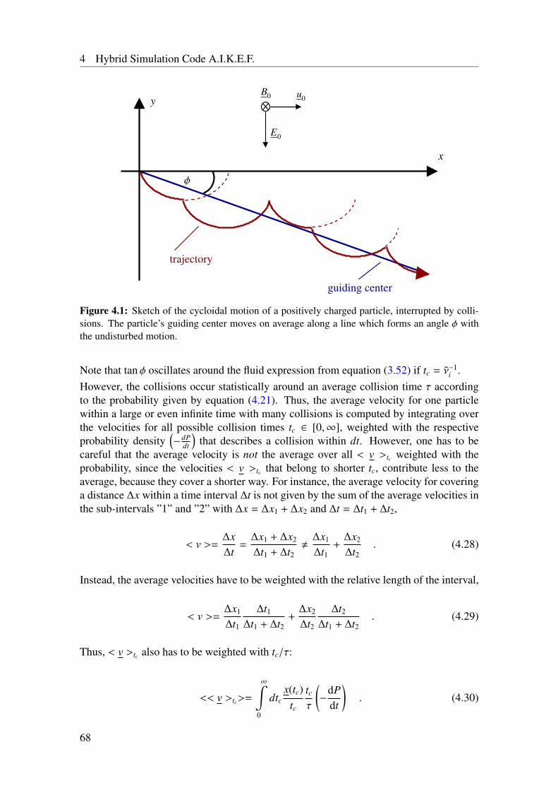
4 Hybrid Simulation Code A.I.K.E.F.
E0
B0 u0y
x
φ
trajectory
guiding center
Figure 4.1: Sketch of the cycloidal motion of a positively charged particle, interrupted by colli-sions. The particle’s guiding center moves on average along a line which forms an angle φ withthe undisturbed motion.
Note that tan φ oscillates around the fluid expression from equation (3.52) if tc = ν−1i .
However, the collisions occur statistically around an average collision time τ accordingto the probability given by equation (4.21). Thus, the average velocity for one particlewithin a large or even infinite time with many collisions is computed by integrating overthe velocities for all possible collision times tc ∈ [0,∞], weighted with the respectiveprobability density
(−dP
dt
)that describes a collision within dt. However, one has to be
careful that the average velocity is not the average over all < v >tc weighted with theprobability, since the velocities < v >tc that belong to shorter tc, contribute less to theaverage, because they cover a shorter way. For instance, the average velocity for coveringa distance ∆x within a time interval ∆t is not given by the sum of the average velocities inthe sub-intervals ”1” and ”2” with ∆x = ∆x1 + ∆x2 and ∆t = ∆t1 + ∆t2,
< v >=∆x∆t
=∆x1 + ∆x2
∆t1 + ∆t2,
∆x1
∆t1+
∆x2
∆t2. (4.28)
Instead, the average velocities have to be weighted with the relative length of the interval,
< v >=∆x1
∆t1
∆t1
∆t1 + ∆t2+
∆x2
∆t2
∆t2
∆t1 + ∆t2. (4.29)
Thus, < v >tc also has to be weighted with tc/τ:
<< v >tc>=
∞∫0
dtcx(tc)
tc
tc
τ
(−
dPdt
). (4.30)
68
4.3 Collisions, Reactions and Ionization
Inserting equations (4.24) and (4.20) into (4.30) finally yields
<< vx >tc> =
∞∫0
dtcrg(Ωtc − sin Ωtc)1τ2 exp
(−
tc
τ
)= u0
Ω2
1/τ2 + Ω2 (4.31)
and
<< vy >tc> =
∞∫0
dtcrg(cos Ωtc − 1)1τ2 exp
(−
tc
τ
)= −u0
Ω/τ
1/τ2 + Ω2 . (4.32)
These velocities are exactly the same as the drift velocities obtained from the fluid ap-proach trough Pedersen and Hall currents in section 3.2.4 (equations (3.50) and (3.51)),if τ is replaced by the inverse collision frequency, τ = ν−1
i . Therefore, the statistical de-scription of the collisions is a microscopic model of Pedersen and Hall conductivities andthe drag force.
4.3.3 Photoionization and Electron Impact Ionization
The model includes photoionization and electron impact ionization as described by equa-tions (4.18) and (4.19), respectively. For both processes, new ions are inserted into thesimulation during each time step according to
∂tni(x) = νio(x)nn(x) , (4.33)
where νio(x) denotes the ionization frequency with contributions from photoionization(νph), electron impact ionization (νe) and a possible additional effective ionization fre-quency ν∗ (see section 6.1.3),
νio(x) = νph + νe + ν∗ . (4.34)
The values used for the ionization frequencies are discussed in sections 5.4.1 and 6.1.3.The initial velocity of the newly generated ions is given by the neutral velocity un(x) andsuperimposed random velocities components according to thermal fluctuations.Two different implementations of these ion production processes are included in A.I.K.E.F.:
1. The ”rejection-method”: a certain number N of macroparticles is inserted into thesimulation (typically N ∼ 103) during each ∆t. For each particle, coordinates xwithin the simulation box are generated as random numbers. The coordinates of aparticle are rejected and new coordinates generated as long as
J(x)Jmax
νio(x)nn(x)νio,maxnn,max
< r (4.35)
69
4 Hybrid Simulation Code A.I.K.E.F.
with r ∈ [0; 1] being another random number. In this way, the coordinates thatare most likely generated correspond to the location of the highest ion production.The subscript ’max’ denotes the maximum ion production. J is the determinant ofthe Jacobian matrix, which has to be considered if not Cartesian coordinates, bute.g. spherical coordinates (r, ϑ, ϕ) are generated, since a uniform distribution of theangles ϑ and ϕ does not yield a uniform distribution of the resulting positions. Eachparticle is assigned the same ”weight” w, i.e. each particle contributes equally to thedensity. This contribution is determined according to the number of new particles(N) and according to the ion production rate integrated over the whole simulationbox,
w =
∫νio(x)nn(x)dV
N∆t . (4.36)
This equation represents the integrated version of equation (4.33) for N particleswith equal weight w. Therefore, the rejection method is most suitable in caseswhere νio(x) and nn(x) are defined by analytical expressions and the integral canbe evaluated. The advantage of this method is that it generates a high number ofmacroparticles in the few cells with high ion production rate – which are typicallythe regions of particular interest – and less particles elsewhere.
2. The second possibility is to inject exact one macroparticle in each cell, but dropthe claim that all particles are generate with an equal weight. Instead, each parti-cle’s contribution to the density shall be defined by νio(x) · nn(x). The coordinatesof the particle within the cell are chosen randomly. This method has the advan-tage that only the local values νio(x) and nn(x) are required instead of an integratedquantity. However, in regions of high neutral density the ions are represented bya significantly lower number of macroparticles compared to the rejection method.In contrast, particles are also inserted in regions with low neutral density what maynot be the case for the rejection method. Furthermore, the number of cells is usuallymuch larger than 103 and the resulting high total number of macroparticles woulddrastically slow down the simulation. Therefore, the method is adjusted such thatthe probability to insert a macroparticle is set to k−1, with k > 1. If the particle isinserted, its contribution to the density is consequently increased by the factor k.By adjusting the value of k a similar number of new macroparticles is produced asby the rejection method.
Within this thesis, both methods have been used for the ionization processes in Enceladus’plume: the rejection method has been applied for the simulations presented in chapter 5,where an analytical model of the plume has been used while the second implementationwas more suitable for the simulated neutral plumes in chapter 6. With regard to possiblefuture improvements – like an electron impact ionization rate which changes during thesimulation runtime according to the local electron density – the second implementationshould be preferred.
70
4.4 Numerical Damping (Smoothing)
4.4 Numerical Damping (Smoothing)
As mentioned in section 4.2, it is necessary to apply a smoothing procedure in order toimprove the numerical stability. On the one hand, the smoothing avoids too strong localgradients in the electromagnetic fields. On the other hand, structures with characteristiclength scales comparable to or smaller than the grid size cannot be described correctlywithin the model and therefore, these structures have to be damped.The smoothing of a scalar quantity A[i, j,k] at a grid node [i, j, k] (i, j, k ∈ Z) can be carriedout in two ways (see also Bagdonat [2004]):
1. A ’simple’ smoothing procedure where an average of the fields at the neighbor gridpoints (A[i, j,k]) is added to A[i, j,k] at each grid node according to
Anew[i, j,k] = (1 − ηsm)A[i, j,k] + ηsm A[i, j,k] (4.37)
with
A[i, j,k] =
1∑a,b,c=−1
A[i+a, j+b,k+c] W[a,b,c] (4.38)
and the weighting factors
W[a,b,c] =18
2−(a2+b2+c2) . (4.39)
These factors take into account, how far a node [i + a, j + b, k + c] with a, b, c ∈−1, 0, 1 is away from the node [i, j, k] (see fig. 3.10 of Simon [2007]). The strengthof the smoothing is determined by the parameter ηsm.
2. The second possibility is the use of a small, global value of η in the diffusion termof equation (A), in addition to the resistivity of the obstacle. Physically, a value ofη different from zero would be the result of wave-particle scattering or electron-ioncollisions. For numerical stability, η has to be chosen somewhat larger than the realvalue.
Before the impact of the smoothing on the results presented in this thesis is analyzed, itmay be instructive to compare the two smoothing procedures. As has been pointed outby Müller et al. [2011], the simple smoothing procedure is similar to a Laplace operatorin finite differences and therefore acts in a similar manner as diffusion. Since A.I.K.E.F.is currently used by a large number of people, it may be of some interest to learn aboutthe smoothing strength of the two methods relative to each other, i.e. to find a relationbetween the smoothing parameters ηsm and η.On the one hand, rewriting equation (4.37) yields
Anew[i, j,k] = A[i, j,k] − ηsm · f (A[i, j,k]) , (4.40)
where the abbreviation f (A[i, j,k]) = A[i, j,k] − A[i, j,k] has been introduced. On the other hand,the diffusion term in the magnetic field equation reads
∂tB = −∂x ×
(η
µ0∂x × B
). (4.41)
71
4 Hybrid Simulation Code A.I.K.E.F.
Rewritten for discrete time steps one obtains
Bt+∆t − Bt
∆t= −∂x ×
(η
µ0∂x × Bt
)(4.42)
andBt+∆t = Bt −
η∆tµ0
(∂x × (∂x × Bt)
). (4.43)
In the last step, η is assumed to be constant, i. e. η , η(x). With ∂x · B = 0, it is∂x × (∂x × B) = −∂2
xB. The spatial derivatives in finite differences for the components ofB at grid node [i, j, k] for an equidistant Cartesian grid yield for, e.g. the Bx component,
Bt+∆tx,[i, j,k] = Bt
x,[i, j,k] +η∆tµ0
Btx,[i+1, j,k] − 2Bt
x,[i, j,k] + Btx,[i−1, j,k]
∆x2
Btx,[i, j+1,k] − 2Bt
x,[i, j,k] + Btx,[i, j−1,k]
∆x2
Btx,[i, j,k+1] − 2Bt
x,[i, j,k] + Btx,[i, j,k−1]
∆x2
. (4.44)
For formal analogy to equation (4.40), this expression is rewritten as
Bt+∆tx,[i, j,k] = Bt
x,[i, j,k] −η∆tµ0∆x2
Btx,[i, j,k] −
1∑a,b,c=−1
B[i+a, j+b,k+c] W[a,b,c]
= Bt
x,[i, j,k] −η∆tµ0∆x2
(Bt
x,[i, j,k] − Btx,[i, j,k])
)= Bt
x,[i, j,k] −η∆tµ0∆x2 g(Bt
x,[i, j,k]) , (4.45)
where the new weighting factors
W[a,b,c] = δa0δb0 + δb0δc0 + δa0δc0 − 8 δa0δb0δc0 (4.46)
have been introduced. δab denotes the Kronecker-delta. The average Btx,[i, j,k] and the ab-
breviation g(Btx,[i, j,k]) = Bt
x,[i, j,k] − Btx,[i, j,k] are introduced in analogy to equation (4.40).
By comparing equations (4.40) and (4.45), one may identify
ηsm =η∆tµ0∆x2 =
η∗∆t∗
(∆x∗)2 (4.47)
where the quantities (...)∗ correspond to normalized units with η∗ = ηen0/B0. Therefore,the smoothing parameter ηsm depends on grid resolution and time step if a similar amountof numerical diffusion should be achieved. Note that in the diffusion term, only the sixnearest neighbors of a node are considered, while the ’simple’ smoothing includes 26neighbors. One should also keep in mind that A.I.K.E.F. advances the diffusion term intime using an implicit Crank-Nicolson algorithm, whereas the explicit Euler method hasbeen used in the derivation of equation (4.45) for simplicity (see section 4.2).
72
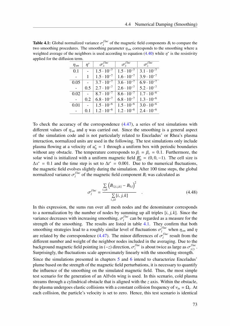
4.4 Numerical Damping (Smoothing)
Table 4.1: Global normalized variance σ f lucl of the magnetic field components Bl to compare the
two smoothing procedures. The smoothing parameter ηsm corresponds to the smoothing where aweighted average of the neighbors is used according to equation (4.40) while η∗ is the resistivityapplied for the diffusion term.
ηsm η∗ σf lucx σ
f lucy σ
f lucz
0.1 - 1.5 · 10−7 1.5 · 10−7 3.1 · 10−7
- 1 1.5 · 10−7 1.6 · 10−7 3.9 · 10−7
0.05 - 3.7 · 10−7 3.6 · 10−7 6.9 · 10−7
- 0.5 2.7 · 10−7 2.6 · 10−7 5.2 · 10−7
0.02 - 8.7 · 10−7 8.6 · 10−7 1.7 · 10−6
- 0.2 6.8 · 10−7 6.8 · 10−7 1.3 · 10−6
0.01 - 1.5 · 10−6 1.5 · 10−6 3.0 · 10−6
- 0.1 1.2 · 10−6 1.2 · 10−6 2.4 · 10−6
To check the accuracy of the correspondence (4.47), a series of test simulations withdifferent values of ηsm and η was carried out. Since the smoothing is a general aspectof the simulation code and is not particularly related to Enceladus’ or Rhea’s plasmainteraction, normalized units are used in the following. The test simulations only includeplasma flowing at a velocity of u∗0 = 1 through a uniform box with periodic boundarieswithout any obstacle. The temperature corresponds to βi = βe = 0.1. Furthermore, thesolar wind is initialized with a uniform magnetic field B∗0 = (0, 0,−1). The cell size is∆x∗ = 0.1 and the time step is set to ∆t∗ = 0.001. Due to the numerical fluctuations,the magnetic field evolves slightly during the simulation. After 100 time steps, the globalnormalized variance σ f luc
l of the magnetic field component Bl was calculated as
σf lucl =
∑i, j,k
(Bl,[i, j,k] − B0,l
)2
∑i, j,k
[i, j, k]. (4.48)
In this expression, the sums run over all mesh nodes and the denominator correspondsto a normalization by the number of nodes by summing up all triples [i, j, k]. Since thevariance decreases with increasing smoothing, σ f luc
l can be regarded as a measure for thestrength of the smoothing. The results are listed in table 4.1. They confirm that bothsmoothing strategies lead to a roughly similar level of fluctuations σ f luc
l when ηsm and ηare related by the correspondence (4.47). The minor differences of σ f luc
l result from thedifferent number and weight of the neighbor nodes included in the averaging. Due to thebackground magnetic field pointing in (−z) direction, σ f luc
z is about twice as large as σ f lucx/y .
Surprisingly, the fluctuations scale approximately linearly with the smoothing strength.Since the simulations presented in chapters 5 and 6 intend to characterize Enceladus’plume based on the strength of the magnetic field perturbations, it is necessary to quantifythe influence of the smoothing on the simulated magnetic field. Thus, the most simpletest scenario for the generation of an Alfvén wing is used. In this scenario, cold plasmastreams through a cylindrical obstacle that is aligned with the z axis. Within the obstacle,the plasma undergoes elastic collisions with a constant collision frequency of νin = Ωi. Ateach collision, the particle’s velocity is set to zero. Hence, this test scenario is identical
73
4 Hybrid Simulation Code A.I.K.E.F.
to the approach of constant conductances within a cylindrical obstacle, which has beenused for the derivation of the analytical solution of the Alfvén wing (cf. section 3.2.5).This test scenario therefore allows a quantitative comparison between simulations andanalytical solution and will also be applied in sections 4.5.2 and 5.3.In agreement with our default Enceladus parameters listed in table 2.4, the density of theplasma is n0 = 70.5 cm−3, the background magnetic field is given by B0 = (0, 0,−325 nT),the velocity is u0 = 26.4 km/s and the ion mass is 17.6 amu. The size of the simulationbox is Lx × Ly × Lz = 30RE × 25RE × 100RE, since it is adjusted to the nearly field-aligned Alfvén wing. A uniform grid with a cell size of ∆x = 0.26RE is applied. To avoidany boundary effects (see section 4.5.2), the simulation is not run until stationarity, butstopped before the Alfvén wing can reach the top and bottom boundaries of the box, i.e.the simulation time is τ = τA = 40RE/vA ≈ 90 s. The radius and the height of the cylinderare set to 2RE, yielding height-integrated conductivities of
ΣP = ΣH =
2RE∫0
dzneB0
12
= 8.8 S .
From equations (3.87) and (3.88) the Bx and By perturbations inside the flux tube of thenorthern Alfvén wing can then be calculated to
Bx = −0.6MAB0 , By = 0.2MAB0 .
These theoretical perturbations for an ideal Alfvén wing will now be compared with simu-lation results for different values of the smoothing resistivity (η∗ ∈ 0.01, 0.02, 0.05, 0.1).For convenience, the resistivity is provided in normalized units, the corresponding SIunits can be obtained from η = η∗B0/(en0). Figure 4.2(a) shows the Bx perturbation inthe northern Alfvén wing for a smoothing of η∗ = 0.05. To enable a more quantitativeanalysis, the Bx perturbations for the different strengths of the smoothing are compared infigure 4.2(b) along the northern Alfvén characteristic (black line in panel (a)). In all foursimulations, the perturbation is strongest at z = 5RE which results from contributions ofthe Pedersen and Hall currents. The weaker perturbations at z > 30RE result from Alfvénwaves that are generated at the begin of the simulation when the plasma flow within theobstacle has not yet been slowed down to the stationary values. Therefore, the region atz > 30RE could be regarded as the front of the Alfvén wing, which is, however, not partof the stationary solution. Only in between, i.e. from about z = 10RE to z = 25RE, theresults should be compared with the Alfvén wing far field solution. For the two lowestsmoothing values of η∗ = 0.01 (red line) and η∗ = 0.02 (blue line), the simulated fieldperturbations are very close to the analytical value. For a resistivity of η∗ = 0.05, themagnitude of Bx is reduced by about 10% and Bx is not constant along the characteristic,but exhibits a stronger gradient towards larger z. The strongest smoothing even leads to adecrease of the Bx perturbation to Bx = −0.45MAB0 at z = 25RE, i.e. a reduction by about25% compared to the analytical value.These results suggest to choose the resistivity smaller or equal than η∗ = 0.02 to avoid anynoticeable influence of the smoothing on the results. However, the Enceladus simulationsincluding the solid body and the plume have proven to require a smoothing of at leastη∗ = 0.05 for numerical stability. Thus, when interpreting the simulation results, it has to
74
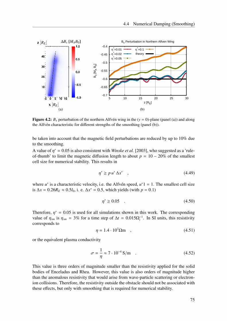
4.4 Numerical Damping (Smoothing)
x [RE ]
z [RE ] ∆Bx [MAB0]
1
(a)
-0.7
-0.65
-0.6
-0.55
-0.5
-0.45
-0.4
5 10 15 20 25 30B
x [M
A B
0]
z [RE]
Bx Perturbation in Northern Alfven Wing
η*=0.01
η*=0.02
η*=0.05
η*=0.1theory
(b)
Figure 4.2: Bx perturbation of the northern Alfvén wing in the (y = 0)-plane (panel (a)) and alongthe Alfvén characteristic for different strengths of the smoothing (panel (b)).
be taken into account that the magnetic field perturbations are reduced by up to 10% dueto the smoothing.A value of η∗ = 0.05 is also consistent with Winske et al. [2003], who suggested as a ’rule-of-thumb’ to limit the magnetic diffusion length to about p = 10 − 20% of the smallestcell size for numerical stability. This results in
η∗ ≥ p u∗ ∆x∗ , (4.49)
where u∗ is a characteristic velocity, i.e. the Alfvén speed, u∗1 = 1. The smallest cell sizeis ∆x = 0.26RE ≈ 0.5l0, i. e. ∆x∗ = 0.5, which yields (with p = 0.1)
η∗ ≥ 0.05 . (4.50)
Therefore, η∗ = 0.05 is used for all simulations shown in this work. The correspondingvalue of ηsm is ηsm = 3% for a time step of ∆t = 0.015Ω−1
i . In SI units, this resistivitycorresponds to
η = 1.4 · 103Ωm , (4.51)
or the equivalent plasma conductivity
σ =1η≈ 7 · 10−4 S/m . (4.52)
This value is three orders of magnitude smaller than the resistivity applied for the solidbodies of Enceladus and Rhea. However, this value is also orders of magnitude higherthan the anomalous resistivity that would arise from wave-particle scattering or electron-ion collisions. Therefore, the resistivity outside the obstacle should not be associated withthese effects, but only with smoothing that is required for numerical stability.
75
4 Hybrid Simulation Code A.I.K.E.F.
4.5 Boundary Conditions
The boundary conditions applied within a simulation may have an even stronger influenceon the results than the smoothing. In general, there are two types of boundaries that haveto be handled by the code: the inner boundary at the surface of the solid obstacle and theouter boundaries which confine the simulation box.
4.5.1 Inner boundary
The inner boundary has already been described in detail by Kriegel et al. [2009]. Onthe one hand, every particle, which impinges on the surface of the moon’s solid body,is removed from the simulation. On the other hand, no boundary condition is appliedto the electromagnetic fields. E and B are calculated self-consistently from the hybridequations within the entire computational domain including the interior of the satellite.The distinction between the exterior and the interior is exclusively controlled by ui , ρi
and η. The velocity ui and the reciprocal density 1/ρi are set to zero within the obstacle.For numerical reasons, however, a discontinuity in the density cannot be handled by thecode. Thus, only for the calculation of the fields, we set the density in the interior to thevery low value of 1 ·10−6 ·n0∗. In order to avoid a strong resistivity gradient at the surface,we apply a resistivity profile with a continuous transition from η = 0 (or η = const in caseit is also used as smoothing) in the plasma to a finite resistivity η0 in the moon’s interior.This continuous resistivity profile is either realized by smearing out the constant resis-tivity of the interior by means of repeated smoothing of the resistivity at the begin of thesimulation (equation (4.40)) or by setting η(x) according to a spherically symmetric Fermiprofile,
η(r) = η01
exp[(r − Rη) aη
]+ 1
. (4.53)
On the one hand, the parameters Rη and aη have to be adjusted such that the artificialresistivity outside the obstacle is as small as possible. On the other hand, too sharp gradi-ents destabilize the field solvers and may require very small time steps. Therefore, theseparameters have to be chosen carefully for a good trade-off between simulation time andartificial plasma resistivity.The modeling of the moons’ interior as described above assumes that these objects couldbe described by a homogeneous resistivity. As has already been discussed in section 3.1,the icy moons’ nearly insulating crusts are the reason why they can be described – understationary conditions – as homogeneous low-conducting obstacles. The value of η0 or thecorresponding conductivity could be specified from two points of view. First, measure-ments of the electrical properties of the surfaces in principle constrain the conductivityof the crusts. However, the available measurements yield a wide range of possible con-ductivities, e.g. pure water ice has a conductivity of the order of σice ∼ 10−9 S/m buteven minor impurities may increase the conductivity by orders of magnitude. Second, themagnetic field should diffuse freely through the satellites and therefore, the conductivityof the obstacles has to be chosen such that the magnetic diffusion time inside the obstacles
76

4.5 Boundary Conditions
E3 E5
x [RE ]
z [RE ] ni [cm−3]
1
(a)
E3 E5
x [RE ]
z [RE ] ni [cm−3]
1
(b)
0
10
20
30
40
50
60
70
-2 -1.5 -1 -0.5 0 0.5 1 1.5 2
η [η
0]
r [RE]
Profile of Resisitivity η
WITH solid bodyWITHOUT solid body: η=0.05η0
(c)
−30
−20
−10
0
10
13:48 13:50 13:52 13:54 13:56 13:58
Magnetic Field − E14 (01 Oct 2011 DOY274) C/A: 95 km at UTC 13:52:26
∆Bx [nT]
−25
−20
−15
−10
−5
0
5
13:48 13:50 13:52 13:54 13:56 13:58
∆By [nT]
−20
−15
−10
−5
0
5
13:48 13:50 13:52 13:54 13:56 13:58UTCx [RE]y [RE]z [RE]
−3.0−7.2−1.3
−1.7−4.0−1.3
−0.3−0.7−1.4
+1.1+2.5−1.4
+2.6+5.7−1.4
+4.1+8.9−1.4
∆Bz [nT]
Cassini MAG
WITH solid body
WITHOUT solid body
(d)
Figure 4.3: Test of the inner boundary for the Enceladus simulations. Two simulations are shown:(1) including Enceladus as solid obstacle, the resulting ion density is displayed in panel (a), (2)without solid obstacle, the corresponding density is shown in panel (b). Plot (c) displays theresistivity profiles. Plot (d) shows simulated magnetic field components for the E14 flyby.
is significantly smaller than the plasma convection time around it,
τdi f f ≈ µ0σ(2R j
)2 τconv ≈
2R j
u0, (4.54)
where R j denotes the radius of the respective satellite ( j = E,RH). For both satellites, thiscondition is fulfilled for a conductivity of the order of σ ∼ 10−7 S/m, what is also closeto estimates for the Terrestrial moon. In consequence, a conductivity of σ = 7 · 10−7 S/mis used for all Enceladus simulations presented in this thesis, whereas a value of σ =
9 · 10−7 S/m is applied for Rhea.It should be pointed out that for any simulation scenario, it has to be carefully checkedwhether and how much the resistivity profile affects the results. To compare the plasmastructures generated by the resistive obstacle with the effect of an ionosphere, either ofthem could be disabled for test simulation purposes. For Enceladus, such a comparisonis shown in figure 4.3. Two simulations are compared with each other: (1) an Enceladussimulation with parameters as described in chapter 6. The resulting ion density is zeroinside the moon and increased in the plume (panel 4.3(a), see also figure 6.7(c)). Theresistivity profile is described by the solid red line in plot 4.3(c). (2) the same simulationexcept that no solid obstacle is included. Therefore, no effect of the moon on the iondensity is visible (cf. panel 4.3(b)). Moreover, the resistivity is now constant, η = 0.05η0.As an example, panel 4.3(d) displays the resulting magnetic field perturbations along theE14 trajectory for both simulations. The physics of these magnetic field signatures will bediscussed in section 6.5.3; here it is only important to notice that the simulated magnetic
77
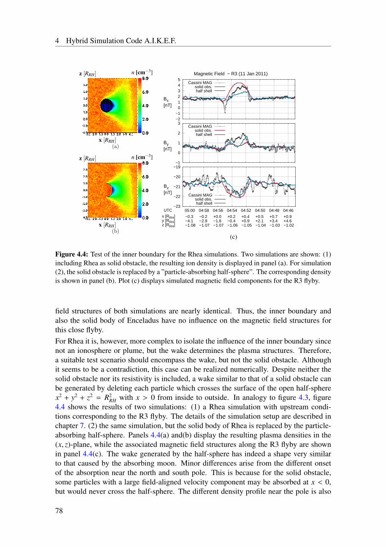
4 Hybrid Simulation Code A.I.K.E.F.
x [RRH]
z [RRH] n [cm−3]
1
(a)
x [RRH]
z [RRH] n [cm−3]
1
(b)
−2−1 0 1 2 3 4 5
04:4604:4804:5004:5204:5404:5604:5805:00
Magnetic Field − R3 (11 Jan 2011)
Bx [nT]
Cassini MAGsolid obs.half shell
−1
0
1
2
3
04:4604:4804:5004:5204:5404:5604:5805:00
By [nT]
Cassini MAGsolid obs.half shell
−23
−22
−21
−20
−19
04:4604:4804:5004:5204:5404:5604:5805:00UTCx [RRH]y [RRH]z [RRH]
+0.9+4.6−1.02
+0.7+3.4−1.03
+0.5+2.1−1.04
+0.4+0.9−1.05
+0.2−0.4−1.06
+0.0−1.6−1.07
−0.2−2.9−1.07
−0.3−4.1−1.08
Bz [nT] Cassini MAG
solid obs.half shell
(c)
Figure 4.4: Test of the inner boundary for the Rhea simulations. Two simulations are shown: (1)including Rhea as solid obstacle, the resulting ion density is displayed in panel (a). For simulation(2), the solid obstacle is replaced by a ”particle-absorbing half-sphere”. The corresponding densityis shown in panel (b). Plot (c) displays simulated magnetic field components for the R3 flyby.
field structures of both simulations are nearly identical. Thus, the inner boundary andalso the solid body of Enceladus have no influence on the magnetic field structures forthis close flyby.For Rhea it is, however, more complex to isolate the influence of the inner boundary sincenot an ionosphere or plume, but the wake determines the plasma structures. Therefore,a suitable test scenario should encompass the wake, but not the solid obstacle. Althoughit seems to be a contradiction, this case can be realized numerically. Despite neither thesolid obstacle nor its resistivity is included, a wake similar to that of a solid obstacle canbe generated by deleting each particle which crosses the surface of the open half-spherex2 + y2 + z2 = R2
RH with x > 0 from inside to outside. In analogy to figure 4.3, figure4.4 shows the results of two simulations: (1) a Rhea simulation with upstream condi-tions corresponding to the R3 flyby. The details of the simulation setup are described inchapter 7. (2) the same simulation, but the solid body of Rhea is replaced by the particle-absorbing half-sphere. Panels 4.4(a) and(b) display the resulting plasma densities in the(x, z)-plane, while the associated magnetic field structures along the R3 flyby are shownin panel 4.4(c). The wake generated by the half-sphere has indeed a shape very similarto that caused by the absorbing moon. Minor differences arise from the different onsetof the absorption near the north and south pole. This is because for the solid obstacle,some particles with a large field-aligned velocity component may be absorbed at x < 0,but would never cross the half-sphere. The different density profile near the pole is also
78
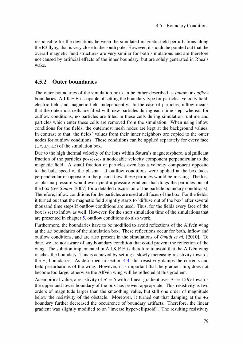
4.5 Boundary Conditions
responsible for the deviations between the simulated magnetic field perturbations alongthe R3 flyby, that is very close to the south pole. However, it should be pointed out that theoverall magnetic field structures are very similar for both simulations and are thereforenot caused by artificial effects of the inner boundary, but are solely generated in Rhea’swake.
4.5.2 Outer boundaries
The outer boundaries of the simulation box can be either described as inflow or outflowboundaries. A.I.K.E.F. is capable of setting the boundary type for particles, velocity field,electric field and magnetic field independently. In the case of particles, inflow meansthat the outermost cells are filled with new particles during each time step, whereas foroutflow conditions, no particles are filled in these cells during simulation runtime andparticles which enter these cells are removed from the simulation. When using inflowconditions for the fields, the outermost mesh nodes are kept at the background values.In contrast to that, the fields’ values from their inner neighbors are copied to the outernodes for outflow conditions. These conditions can be applied separately for every face(±x,±y,±z) of the simulation box.Due to the high thermal velocity of the ions within Saturn’s magnetosphere, a significantfraction of the particles possesses a noticeable velocity component perpendicular to themagnetic field. A small fraction of particles even has a velocity component oppositeto the bulk speed of the plasma. If outflow conditions were applied at the box facesperpendicular or opposite to the plasma flow, these particles would be missing. The lossof plasma pressure would even yield a pressure gradient that drags the particles out ofthe box (see Simon [2007] for a detailed discussion of the particle boundary conditions).Therefore, inflow conditions for the particles are used at all faces of the box. For the fields,it turned out that the magnetic field slightly starts to ’diffuse out of the box’ after severalthousand time steps if outflow conditions are used. Thus, for the fields every face of thebox is set to inflow as well. However, for the short simulation time of the simulations thatare presented in chapter 5, outflow conditions do also work.Furthermore, the boundaries have to be modified to avoid reflections of the Alfvén wingat the ±z boundaries of the simulation box. These reflections occur for both, inflow andoutflow conditions, and are also present in the simulations of Omidi et al. [2010]. Todate, we are not aware of any boundary condition that could prevent the reflection of thewing. The solution implemented in A.I.K.E.F. is therefore to avoid that the Alfvén wingreaches the boundary. This is achieved by setting a slowly increasing resistivity towardsthe ±z boundaries. As described in section 4.4, this resistivity damps the currents andfield perturbations of the wing. However, it is important that the gradient in η does notbecome too large, otherwise the Alfvén wing will be reflected at this gradient.As empirical value, a resistivity of η∗ = 5 with a linear gradient over ∆z = 15RE towardsthe upper and lower boundary of the box has proven appropriate. This resistivity is twoorders of magnitude larger than the smoothing value, but still one order of magnitudebelow the resistivity of the obstacle. Moreover, it turned out that damping at the +xboundary further decreased the occurrence of boundary artifacts. Therefore, the lineargradient was slightly modified to an ”inverse hyper-ellipsoid”. The resulting resistivity
79
4 Hybrid Simulation Code A.I.K.E.F.
x [RE ]
z [RE ] η [η0]
1
(a)
x [RE ]
z [RE ] ∆Bx [MAB0]
1
(b)
x [RE ]
z [RE ] ∆Bx [MAB0]
1
(c)
-0.7
-0.65
-0.6
-0.55
-0.5
-0.45
-0.4
-0.35
-0.3
-0.25
5 10 15 20 25 30
Bx
[MA B
0]
z [RE]
Bx Perturbation in Northern Alfven Wing
t=τA
t=τA, η-Boundary
t=3τA
t=3τA, η-Boundary
(d)
Figure 4.5: Modified boundary with increased resistivity near the ±z boundaries (panel (a)) toavoid reflections of the Alfvén wing. Plot (b) shows the Bx perturbation of a simulation withoutthe modified boundary where the Alfvén wing is reflected, while panel (c) displays a run where theAlfvén wing is damped by the increased η. Panel (d) shows a comparison of the two simulationsalong the Alfvén characteristic (black lines in (b) and (c)) before (t = τA) and after (t = 3τA) theAlfvén wing is reflected.
distribution is shown in figure 4.5(a).To investigate how strong this modified boundary impacts the plasma structures, againthe field perturbations within the Alfvén wing are considered. The same basic scenarioto generate an Alfvén wing is applied as in the analysis of the smoothing in section 4.4,but now including the resistive boundary. This simulation, however, is not stopped beforethe Alfvén wing reaches the boundary, but run three times longer (τ = 3τA ≈ 270 s).The resulting Bx perturbation in the northern Alfvén wing is shown in figure 4.5(b) for asimulation without the modified boundary and in panel 4.5(c) for a simulation includingthis resistive boundary. The reflected Alfvén wing is clearly visible in figure 4.5(b) as
80
4.6 Further Simulation Codes for Enceladus and Rhea
the region of positive Bx at about x = 10RE. In contrast, no reflected wing can be seenin plot 4.5(c). For a quantitative analysis, the Bx perturbations are also shown along theAlfvén characteristic in figure 4.5(d). The two simulations are shown before the Alfvénwing reaches the boundary, i.e. after t = τA, and also after the reflection has occurred atthe time t = 3τA. Northward of z = 12RE, the increased resistivity leads to the desireddamping of the Bx perturbation. For the simulation without increased resistivity, the su-perposition of the original and the reflected wing also leads to a reduced Bx perturbation atz > 20RE. Interestingly, both simulation produce at t = 3τA a slightly larger perturbation.Most important is, however, the fact that the simulation including the resistive boundarygenerates a similar perturbation close to the obstacle and does prevent the reflection ofthe wing. Thus, this resistive boundary is an appropriate choice for modeling stationaryAlfvén wing structures within a finite-sized simulation box.
4.6 Further Simulation Codes for Enceladus and Rhea
Finally, A.I.K.E.F. shall be compared with other existing simulation codes that have beenapplied to the plasma interactions of Enceladus and Rhea.In the case of Rhea, only the ”Braunschweig-Code” has been used for simulations ofRhea’s plasma environment [Roussos et al. 2008a]. It turned out that the A.I.K.E.F.’s innerboundary condition – which was already implemented in that version of the Braunschweig-Code – is particularly suitable to model the inert moons. In contrast, Enceladus has beenmodeled by a number of authors apart from our preceding study [Kriegel et al. 2009].Saur et al. [2008] used an updated version of the two-fluid plasma model of Saur andStrobel [2005] for Enceladus’ plasma interaction. The model calculates the modifica-tions of electron and ion density, velocity, and temperature by aeronomic reactions witha given neutral gas distribution (such as electron impact ionization and charge exchange).The model also computes the 3D electric current system driven by the interaction, fromwhich the associated magnetic field perturbations are calculated by means of Biot-Savart-Integrals [Saur et al. 2002]. Due to the analytical description of the inner boundary, themodel naturally includes the hemisphere coupling currents. Overall, the model of Sauret al. [2008] is similar to first-order perturbation theory and – although producing ex-cellent results – does not self-consistently include the modifications of the plasma flowpatterns by the perturbed magnetic field.A series of hybrid simulation studies of Enceladus’ plasma interaction was carried out byOmidi et al. [2010, 2012]. In contrast to A.I.K.E.F., the hybrid code of these authors isnot capable of using an adaptive or hierarchical mesh. Instead, the calculations are run ona uniform Cartesian grid with massive computational resources to achieve a resolution ofup to 17 km, similar to our model. Furthermore, the initial magnetic field is kept constantwithin the obstacle. In contrast to the assumption of adiabatic electrons in A.I.K.E.F., theelectron pressure is determined assuming isothermal electrons. In addition, Omidi et al.[2010] did not implement a damping of the Alfvén wings near the boundaries. Therefore,their simulations are run only until the Alfvén wing reaches the ±z boundaries of thesimulation box. Similar to our studies, Omidi et al. [2012] included dust as a heavy,negatively charged ion species. While the work presented in this thesis mainly focuses
81
4 Hybrid Simulation Code A.I.K.E.F.
on the magnetic field structures, Omidi et al. [2010, 2012] analyzed wave generation andenergy spectra. Furthermore, these authors did not include a detailed model of the ion-neutral chemistry which will prove necessary for a quantitative comparison with Cassinimagnetometer data.The hybrid code developed by the group of P. Trávnícek from the Space Plasma Groupat the Astronomical Institute of the Academy of Sciences of the Czech Republic has alsobeen applied to Enceladus by Stverak et al. [2009]. These authors, however, did neverpresent their results in a peer-reviewed journal .The MHD simulation code BATS-R-US (Block Adaptive Tree Solar-wind Roe UpwindScheme) developed at the University of Michigan has been applied to Enceladus’ plasmainteraction by Jia et al. [2010b,c,d]. This MHD code uses similar parameters as appliedfor the simulations with A.I.K.E.F., e. g. the simulation domain is 80RE × 80RE × 80RE
which is similar to our model in the z direction, but larger in x and y direction becauseBATS-R-US is only capable of square meshes. By using a multiscale grid system, Jia etal. achieved a resolution of 10 km, which is slightly better than our resolution. In theirmodel, the surface of Enceladus is the inner boundary of the calculation domain. Theplasma is absorbed at Enceladus’ surface, while the gradient of the magnetic field is setto zero across the boundary. From these parameters, BATS-R-US seems to be equallysuitable to study Enceladus’ plasma interaction as A.I.K.E.F. However, the major resultof this thesis is the vital importance of charged dust for the plasma structures. Conse-quently, Jia et al. [2012] applied the multi-fluid version of BATS-R-US to study the effectof charged dust. Although it is in principle possible to include the charged dust evenwithin the MHD framework (see the recent study by Blöcker [2013]), Jia et al. have notyet succeeded to qualitatively explain Cassini MAG observations at Enceladus that areassociated with charged dust.A multi-fluid simulation model has also been applied to Enceladus by Paty et al. [2011].Similar to Jia et al., these authors have not yet successfully included the charged dust andno peer-reviewed publication was available at the time of this writing.In summary, A.I.K.E.F. is due to both, numerical implementation and capabilities inherentto any hybrid model, the only simulation code that has already been successfully appliedto the plasma interactions of Enceladus and Rhea and which is also suitable to address theopen questions arising from measurements in the vicinity of the two moons.
82
5 Influence of Negatively ChargedPlume Grains on the Structure ofEnceladus’ Alfvén Wings
The following chapter has been published in wide parts before submission of the thesis.The copyright holder of the pre-publications is the American Geophysical Union, and thecited parts are reprinted with permission. The publications can be found under the fol-lowing references:Simon, S., J. Saur, H. Kriegel, F. M. Neubauer, U. Motschmann, and M. K. Dougherty(2011a), Influence of negatively charged plume grains and hemisphere coupling currentson the structure of Enceladus’ Alfvén wings: Analytical modeling of Cassini magne-tometer observations, Journal of Geophysical Research (Space Physics), 116, A04221,doi: 10.1029/2010JA016338Kriegel, H., S. Simon, U. Motschmann, J. Saur, F. M. Neubauer, A. M. Persoon, M. K.Dougherty, and D. A. Gurnett (2011), Influence of negatively charged plume grains on thestructure of Enceladus’ Alfvén wings: Hybrid simulations versus Cassini Magnetometerdata, Journal of Geophysical Research (Space Physics), 116, A10223,doi: 10.1029/2011JA016842
5.1 Magnetic Field Observations at Enceladus
At the end of chapter 3, it has been discussed that our previous hybrid simulations aswell as MHD simulations by Jia et al. [2010c] failed to explain some key features ofEnceladus’ plasma interaction like the orientation of the measured By perturbation (atleast within a local interaction model) and the location of draping center. To investigatethese puzzling issues, we will at first discuss the magnetic field signatures obtained dur-ing Cassini’s E5 – E9 and E11 flybys at Enceladus, which are displayed in figure 5.1.For better visualization only the magnetic field perturbations (∆Bx,∆By,∆Bz) caused byEnceladus are shown. To subtract the background field from the data, we have fitted adipole field to the intervals between 10 and 20 minutes before and after closest approach.For all flybys except for E8 and E11, Cassini observed a negative Bx perturbation, indi-cating that the spacecraft passed through the center of the northern Alfvén wing althoughCassini was located below the south pole. This means that Cassini crossed the interac-tion region between the south pole of Enceladus and the draping center. Surprisingly,
83
5 Influence of Dust on Enceladus’ Alfvén Wings
the By perturbations from all these flybys exhibited a negative sign. During E8 and E11,the spacecraft flew through the southern Alfvén wing and the measured magnetic fieldperturbations were positive for both, Bx and By.For the component in the direction of the background field (Bz), only a negative per-turbation was measured during all flybys so far. Since the background field is directedtowards negative z, Cassini passed only through regions of enhanced |B|. In other words,the spacecraft intersected the magnetic pile-up region, but did not penetrate the corre-sponding magnetic field decrease in the downstream region. The step-like shape of the Bz
perturbations of E7 (panel 5.1(c)) results from artifacts caused by the reduced resolutionof the MAG instrument1.The analytical solution for the magnetic field perturbations of the Alfvén wing derived insection 3.2.5 showed that the bending of the field lines yields a negative Bx component inthe northern and a positive Bx within the southern wing flux tube. In addition, the Hallcurrent within the plume gives rise to a component along the Saturn-Enceladus-line (By).In the far field (i.e. where the magnetic field arising from Pedersen and Hall currents canbe neglected), the wing current system and the associated magnetic field perturbationsexhibit translation symmetry along the wing characteristics. This also implies that theorientation of the By component, even at large distances to Enceladus, is determined bythe value of the Hall conductance of the local interaction region. In equations (3.87)– (3.88), the magnetic field perturbations inside the Alfvénic flux tube were given as afunction of the constant height-integrated Pedersen and Hall conductivities ΣP and ΣH
inside a cylindrical plume. According to equation (3.88), the sign of By in the northern orsouthern wing is determined by the sign of the Hall conductance, or more precisely,
ΣH > 0 →
By > 0 and Bx < 0 (northern Alfvén wing)By < 0 and Bx > 0 (southern Alfvén wing)
. (5.1)
Obviously, the measured positive correlation between the signs of the Bx and By pertur-bations seems to contradict the previous understanding of the Alfvén wing.Since E5 – E7 and E9 passed through the center of the plume, the Alfvén wing far fieldsolution is, however, not strictly applicable for these flybys. In contrast, closest approachof E8 and E11 took place far away from the center of the plume, i.e. at distances of 6.3RE
and 10.1RE, respectively. Therefore, the magnetic perturbations measured during theseflybys should correspond to the Alfvén wing far field solution. In turn, it is a reasonableassumption (which was unambiguously confirmed by our simulations), that the signs ofthe Bx and By perturbations observed during E5 – E7 and E9 in the near-field of thenorthern Alfvén wing are identical to the signs of ∆Bx and ∆By in the northern Alfvénwing far field.There are in principle only three possibilities which could explain the observed magneticfield signatures. First, Cassini did not pass through the Alfvénic flux tube, but instead
1As we mentioned in Simon et al. [2011b], the instrument has been in low-resolution mode (with arange of ±10, 000 nT sampled with 14 bits yielding a digital resolution of 1.22 nT) for periapsis and waitedtoo long before the autoranging unit switched it to high-resolution mode (with a range of ±400 nT and acorresponding digital resolution of 49 pT). The observed magnetic field varies in coarse steps in sensorcoordinates. Because of the performed coordinate transformations, the x, y, and z signals mix and producethe artifacts visible in this plot. However, these signatures do not modify the overall features of the observedfield signature, and for our purposes, they are only of minor quantitative relevance.
84
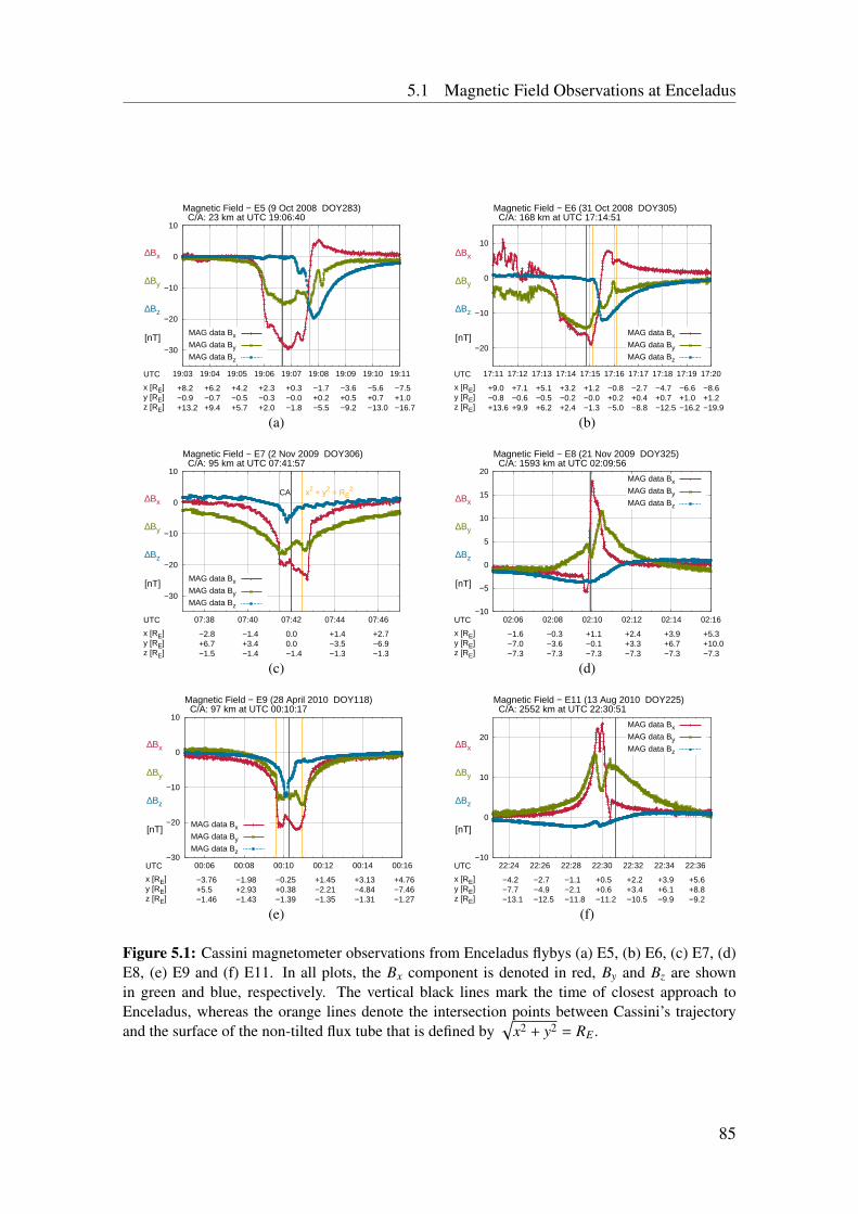
5.1 Magnetic Field Observations at Enceladus
−30
−20
−10
0
10
19:03 19:04 19:05 19:06 19:07 19:08 19:09 19:10 19:11
Magnetic Field − E5 (9 Oct 2008 DOY283) C/A: 23 km at UTC 19:06:40
UTC
x [RE]y [RE]z [RE]
+8.2−0.9+13.2
+6.2−0.7+9.4
+4.2−0.5+5.7
+2.3−0.3+2.0
+0.3−0.0−1.8
−1.7+0.2−5.5
−3.6+0.5−9.2
−5.6+0.7−13.0
−7.5+1.0−16.7
∆Bx
∆By
∆Bz
[nT]MAG data Bx
MAG data By
MAG data Bz
(a)
−20
−10
0
10
17:11 17:12 17:13 17:14 17:15 17:16 17:17 17:18 17:19 17:20
Magnetic Field − E6 (31 Oct 2008 DOY305) C/A: 168 km at UTC 17:14:51
UTC
x [RE]y [RE]z [RE]
+9.0−0.8+13.6
+7.1−0.6+9.9
+5.1−0.5+6.2
+3.2−0.2+2.4
+1.2−0.0−1.3
−0.8+0.2−5.0
−2.7+0.4−8.8
−4.7+0.7−12.5
−6.6+1.0−16.2
−8.6+1.2−19.9
∆Bx
∆By
∆Bz
[nT]MAG data Bx
MAG data By
MAG data Bz
(b)
−30
−20
−10
0
10
07:38 07:40 07:42 07:44 07:46
Magnetic Field − E7 (2 Nov 2009 DOY306) C/A: 95 km at UTC 07:41:57
x2 + y2 = RE2CA
UTC
x [RE]y [RE]z [RE]
−2.8+6.7−1.5
−1.4+3.4−1.4
0.00.0−1.4
+1.4−3.5−1.3
+2.7−6.9−1.3
∆Bx
∆By
∆Bz
[nT]MAG data Bx
MAG data By
MAG data Bz
(c)
−10
−5
0
5
10
15
20
02:06 02:08 02:10 02:12 02:14 02:16
Magnetic Field − E8 (21 Nov 2009 DOY325) C/A: 1593 km at UTC 02:09:56
UTC
x [RE]y [RE]z [RE]
−1.6−7.0−7.3
−0.3−3.6−7.3
+1.1−0.1−7.3
+2.4+3.3−7.3
+3.9+6.7−7.3
+5.3+10.0−7.3
∆Bx
∆By
∆Bz
[nT]
MAG data Bx
MAG data By
MAG data Bz
(d)
−30
−20
−10
0
10
00:06 00:08 00:10 00:12 00:14 00:16
Magnetic Field − E9 (28 April 2010 DOY118) C/A: 97 km at UTC 00:10:17
UTC
x [RE]y [RE]z [RE]
−3.76+5.5−1.46
−1.98+2.93−1.43
−0.25+0.38−1.39
+1.45−2.21−1.35
+3.13−4.84−1.31
+4.76−7.46−1.27
∆Bx
∆By
∆Bz
[nT]MAG data Bx
MAG data By
MAG data Bz
(e)
−10
0
10
20
22:24 22:26 22:28 22:30 22:32 22:34 22:36
Magnetic Field − E11 (13 Aug 2010 DOY225) C/A: 2552 km at UTC 22:30:51
UTC
x [RE]y [RE]z [RE]
−4.2−7.7−13.1
−2.7−4.9−12.5
−1.1−2.1−11.8
+0.5+0.6−11.2
+2.2+3.4−10.5
+3.9+6.1−9.9
+5.6+8.8−9.2
∆Bx
∆By
∆Bz
[nT]
MAG data Bx
MAG data By
MAG data Bz
(f)
Figure 5.1: Cassini magnetometer observations from Enceladus flybys (a) E5, (b) E6, (c) E7, (d)E8, (e) E9 and (f) E11. In all plots, the Bx component is denoted in red, By and Bz are shownin green and blue, respectively. The vertical black lines mark the time of closest approach toEnceladus, whereas the orange lines denote the intersection points between Cassini’s trajectoryand the surface of the non-tilted flux tube that is defined by
√x2 + y2 = RE .
85
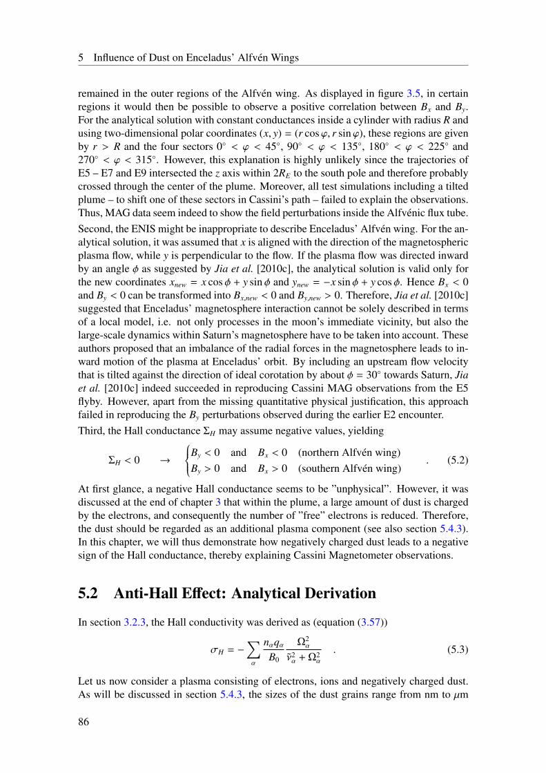
5 Influence of Dust on Enceladus’ Alfvén Wings
remained in the outer regions of the Alfvén wing. As displayed in figure 3.5, in certainregions it would then be possible to observe a positive correlation between Bx and By.For the analytical solution with constant conductances inside a cylinder with radius R andusing two-dimensional polar coordinates (x, y) = (r cosϕ, r sinϕ), these regions are givenby r > R and the four sectors 0 < ϕ < 45, 90 < ϕ < 135, 180 < ϕ < 225 and270 < ϕ < 315. However, this explanation is highly unlikely since the trajectories ofE5 – E7 and E9 intersected the z axis within 2RE to the south pole and therefore probablycrossed through the center of the plume. Moreover, all test simulations including a tiltedplume – to shift one of these sectors in Cassini’s path – failed to explain the observations.Thus, MAG data seem indeed to show the field perturbations inside the Alfvénic flux tube.Second, the ENIS might be inappropriate to describe Enceladus’ Alfvén wing. For the an-alytical solution, it was assumed that x is aligned with the direction of the magnetosphericplasma flow, while y is perpendicular to the flow. If the plasma flow was directed inwardby an angle φ as suggested by Jia et al. [2010c], the analytical solution is valid only forthe new coordinates xnew = x cos φ + y sin φ and ynew = −x sin φ + y cos φ. Hence Bx < 0and By < 0 can be transformed into Bx,new < 0 and By,new > 0. Therefore, Jia et al. [2010c]suggested that Enceladus’ magnetosphere interaction cannot be solely described in termsof a local model, i.e. not only processes in the moon’s immediate vicinity, but also thelarge-scale dynamics within Saturn’s magnetosphere have to be taken into account. Theseauthors proposed that an imbalance of the radial forces in the magnetosphere leads to in-ward motion of the plasma at Enceladus’ orbit. By including an upstream flow velocitythat is tilted against the direction of ideal corotation by about φ = 30 towards Saturn, Jiaet al. [2010c] indeed succeeded in reproducing Cassini MAG observations from the E5flyby. However, apart from the missing quantitative physical justification, this approachfailed in reproducing the By perturbations observed during the earlier E2 encounter.Third, the Hall conductance ΣH may assume negative values, yielding
ΣH < 0 →
By < 0 and Bx < 0 (northern Alfvén wing)By > 0 and Bx > 0 (southern Alfvén wing)
. (5.2)
At first glance, a negative Hall conductance seems to be ”unphysical”. However, it wasdiscussed at the end of chapter 3 that within the plume, a large amount of dust is chargedby the electrons, and consequently the number of ”free” electrons is reduced. Therefore,the dust should be regarded as an additional plasma component (see also section 5.4.3).In this chapter, we will thus demonstrate how negatively charged dust leads to a negativesign of the Hall conductance, thereby explaining Cassini Magnetometer observations.
5.2 Anti-Hall Effect: Analytical Derivation
In section 3.2.3, the Hall conductivity was derived as (equation (3.57))
σH = −∑α
nαqαB0
Ω2α
ν2α + Ω2
α
. (5.3)
Let us now consider a plasma consisting of electrons, ions and negatively charged dust.As will be discussed in section 5.4.3, the sizes of the dust grains range from nm to µm
86
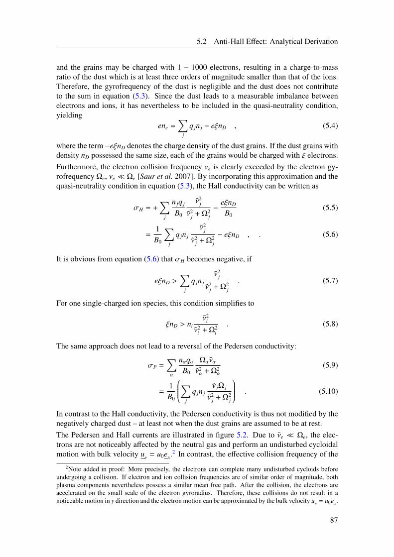
5.2 Anti-Hall Effect: Analytical Derivation
and the grains may be charged with 1 − 1000 electrons, resulting in a charge-to-massratio of the dust which is at least three orders of magnitude smaller than that of the ions.Therefore, the gyrofrequency of the dust is negligible and the dust does not contributeto the sum in equation (5.3). Since the dust leads to a measurable imbalance betweenelectrons and ions, it has nevertheless to be included in the quasi-neutrality condition,yielding
ene =∑
j
q jn j − eξnD , (5.4)
where the term −eξnD denotes the charge density of the dust grains. If the dust grains withdensity nD possessed the same size, each of the grains would be charged with ξ electrons.Furthermore, the electron collision frequency νe is clearly exceeded by the electron gy-rofrequency Ωe, νe Ωe [Saur et al. 2007]. By incorporating this approximation and thequasi-neutrality condition in equation (5.3), the Hall conductivity can be written as
σH = +∑
j
n jq j
B0
ν2j
ν2j + Ω2
j
−eξnD
B0(5.5)
=1B0
∑j
q jn j
ν2j
ν2j + Ω2
j
− eξnD , . (5.6)
It is obvious from equation (5.6) that σH becomes negative, if
eξnD >∑
j
q jn j
ν2j
ν2j + Ω2
j
. (5.7)
For one single-charged ion species, this condition simplifies to
ξnD > niν2
i
ν2i + Ω2
i
. (5.8)
The same approach does not lead to a reversal of the Pedersen conductivity:
σP =∑α
nαqαB0
Ωαναν2α + Ω2
α
(5.9)
=1B0
∑j
q jn jν jΩ j
ν2j + Ω2
j
. (5.10)
In contrast to the Hall conductivity, the Pedersen conductivity is thus not modified by thenegatively charged dust – at least not when the dust grains are assumed to be at rest.The Pedersen and Hall currents are illustrated in figure 5.2. Due to νe Ωe, the elec-trons are not noticeably affected by the neutral gas and perform an undisturbed cycloidalmotion with bulk velocity ue = u0ex.
2 In contrast, the effective collision frequency of the
2Note added in proof: More precisely, the electrons can complete many undisturbed cycloids beforeundergoing a collision. If electron and ion collision frequencies are of similar order of magnitude, bothplasma components nevertheless possess a similar mean free path. After the collision, the electrons areaccelerated on the small scale of the electron gyroradius. Therefore, these collisions do not result in anoticeable motion in y direction and the electron motion can be approximated by the bulk velocity ue = u0ex.
87
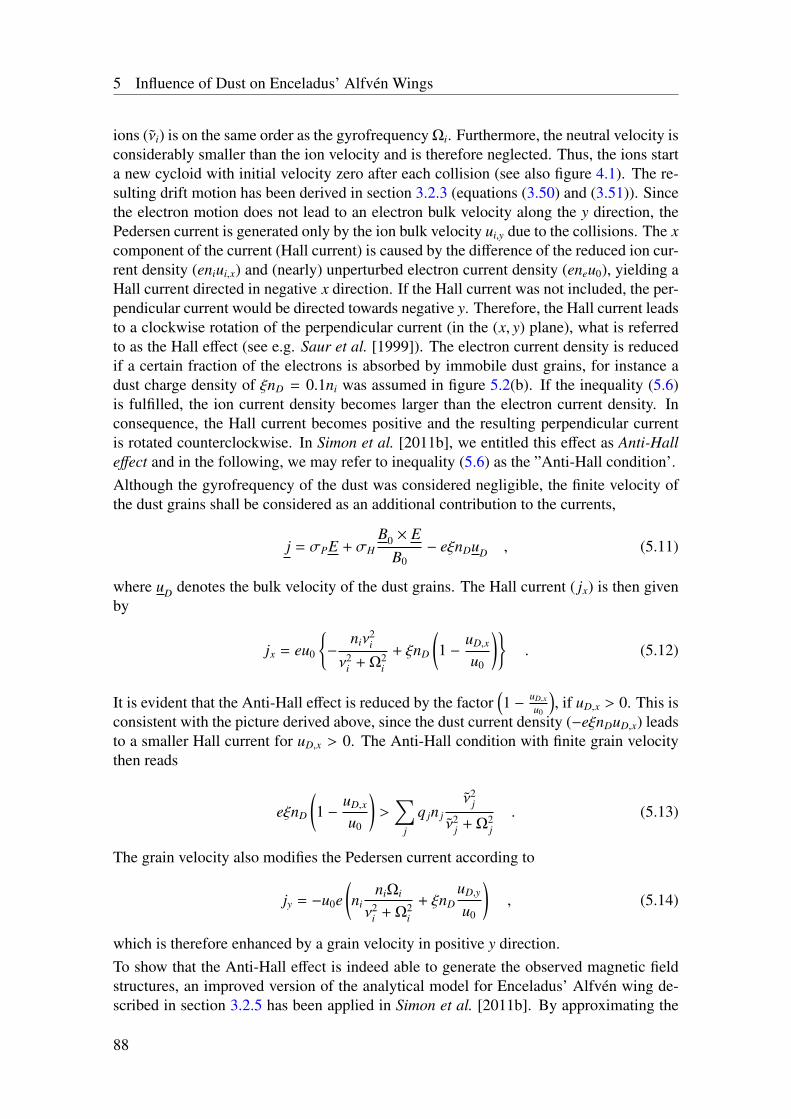
5 Influence of Dust on Enceladus’ Alfvén Wings
ions (νi) is on the same order as the gyrofrequency Ωi. Furthermore, the neutral velocity isconsiderably smaller than the ion velocity and is therefore neglected. Thus, the ions starta new cycloid with initial velocity zero after each collision (see also figure 4.1). The re-sulting drift motion has been derived in section 3.2.3 (equations (3.50) and (3.51)). Sincethe electron motion does not lead to an electron bulk velocity along the y direction, thePedersen current is generated only by the ion bulk velocity ui,y due to the collisions. The xcomponent of the current (Hall current) is caused by the difference of the reduced ion cur-rent density (eniui,x) and (nearly) unperturbed electron current density (eneu0), yielding aHall current directed in negative x direction. If the Hall current was not included, the per-pendicular current would be directed towards negative y. Therefore, the Hall current leadsto a clockwise rotation of the perpendicular current (in the (x, y) plane), what is referredto as the Hall effect (see e.g. Saur et al. [1999]). The electron current density is reducedif a certain fraction of the electrons is absorbed by immobile dust grains, for instance adust charge density of ξnD = 0.1ni was assumed in figure 5.2(b). If the inequality (5.6)is fulfilled, the ion current density becomes larger than the electron current density. Inconsequence, the Hall current becomes positive and the resulting perpendicular currentis rotated counterclockwise. In Simon et al. [2011b], we entitled this effect as Anti-Halleffect and in the following, we may refer to inequality (5.6) as the ”Anti-Hall condition’.Although the gyrofrequency of the dust was considered negligible, the finite velocity ofthe dust grains shall be considered as an additional contribution to the currents,
j = σPE + σHB0 × E
B0− eξnDuD , (5.11)
where uD denotes the bulk velocity of the dust grains. The Hall current ( jx) is then givenby
jx = eu0
−
niν2i
ν2i + Ω2
i
+ ξnD
(1 −
uD,x
u0
). (5.12)
It is evident that the Anti-Hall effect is reduced by the factor(1 − uD,x
u0
), if uD,x > 0. This is
consistent with the picture derived above, since the dust current density (−eξnDuD,x) leadsto a smaller Hall current for uD,x > 0. The Anti-Hall condition with finite grain velocitythen reads
eξnD
(1 −
uD,x
u0
)>
∑j
q jn j
ν2j
ν2j + Ω2
j
. (5.13)
The grain velocity also modifies the Pedersen current according to
jy = −u0e(ni
niΩi
ν2i + Ω2
i
+ ξnDuD,y
u0
), (5.14)
which is therefore enhanced by a grain velocity in positive y direction.To show that the Anti-Hall effect is indeed able to generate the observed magnetic fieldstructures, an improved version of the analytical model for Enceladus’ Alfvén wing de-scribed in section 3.2.5 has been applied in Simon et al. [2011b]. By approximating the
88
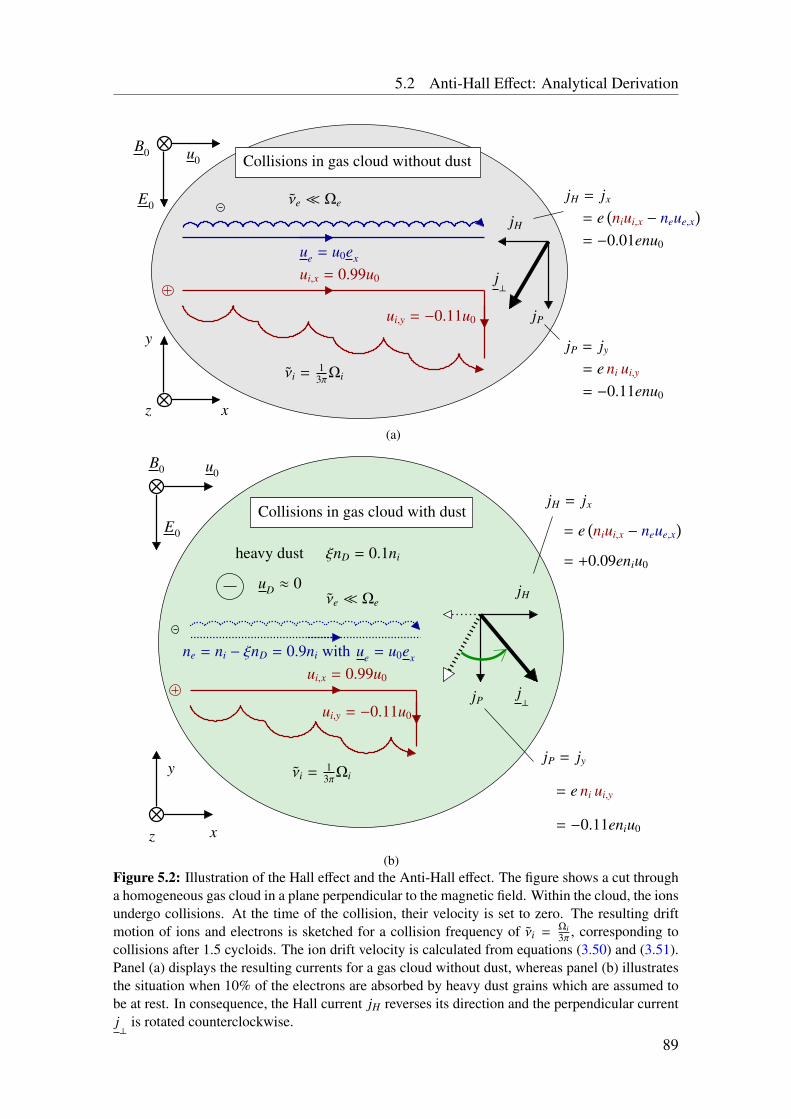
5.2 Anti-Hall Effect: Analytical Derivation
= −0.01enu0
jH = jx
jP = jy
= −0.11enu0
ue = u0ex
νe Ωe
ui,x = 0.99u0
= e(niui,x − neue,x
)
νi = 13πΩi
ui,y = −0.11u0
j⊥
jH
jP
= e ni ui,y
x
B0
E0
u0
y
z
Collisions in gas cloud without dust
(a)
E0
B0
jP = jy
= −0.11eniu0
= e ni ui,y
ui,x = 0.99u0
uD ≈ 0
heavy dust ξnD = 0.1ni
νi = 13πΩi
ne = ni − ξnD = 0.9ni with ue = u0ex
j⊥
νe Ωe
x
= e(niui,x − neue,x
)= +0.09eniu0
jH = jx
y
z
jH
ui,y = −0.11u0
u0
jP
Collisions in gas cloud with dust
(b)Figure 5.2: Illustration of the Hall effect and the Anti-Hall effect. The figure shows a cut througha homogeneous gas cloud in a plane perpendicular to the magnetic field. Within the cloud, the ionsundergo collisions. At the time of the collision, their velocity is set to zero. The resulting driftmotion of ions and electrons is sketched for a collision frequency of νi =
Ωi3π , corresponding to
collisions after 1.5 cycloids. The ion drift velocity is calculated from equations (3.50) and (3.51).Panel (a) displays the resulting currents for a gas cloud without dust, whereas panel (b) illustratesthe situation when 10% of the electrons are absorbed by heavy dust grains which are assumed tobe at rest. In consequence, the Hall current jH reverses its direction and the perpendicular currentj⊥
is rotated counterclockwise.
89
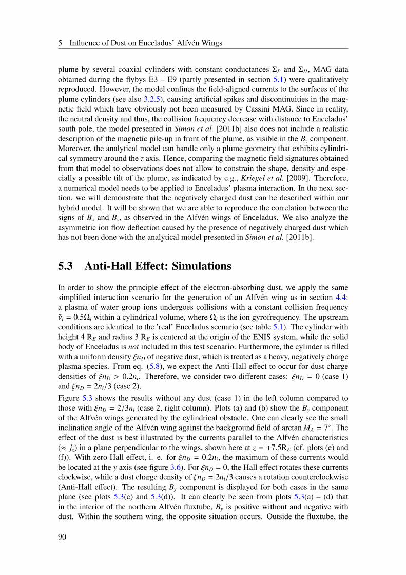
5 Influence of Dust on Enceladus’ Alfvén Wings
plume by several coaxial cylinders with constant conductances ΣP and ΣH, MAG dataobtained during the flybys E3 – E9 (partly presented in section 5.1) were qualitativelyreproduced. However, the model confines the field-aligned currents to the surfaces of theplume cylinders (see also 3.2.5), causing artificial spikes and discontinuities in the mag-netic field which have obviously not been measured by Cassini MAG. Since in reality,the neutral density and thus, the collision frequency decrease with distance to Enceladus’south pole, the model presented in Simon et al. [2011b] also does not include a realisticdescription of the magnetic pile-up in front of the plume, as visible in the Bz component.Moreover, the analytical model can handle only a plume geometry that exhibits cylindri-cal symmetry around the z axis. Hence, comparing the magnetic field signatures obtainedfrom that model to observations does not allow to constrain the shape, density and espe-cially a possible tilt of the plume, as indicated by e.g., Kriegel et al. [2009]. Therefore,a numerical model needs to be applied to Enceladus’ plasma interaction. In the next sec-tion, we will demonstrate that the negatively charged dust can be described within ourhybrid model. It will be shown that we are able to reproduce the correlation between thesigns of Bx and By, as observed in the Alfvén wings of Enceladus. We also analyze theasymmetric ion flow deflection caused by the presence of negatively charged dust whichhas not been done with the analytical model presented in Simon et al. [2011b].
5.3 Anti-Hall Effect: Simulations
In order to show the principle effect of the electron-absorbing dust, we apply the samesimplified interaction scenario for the generation of an Alfvén wing as in section 4.4:a plasma of water group ions undergoes collisions with a constant collision frequencyνi = 0.5Ωi within a cylindrical volume, where Ωi is the ion gyrofrequency. The upstreamconditions are identical to the ’real’ Enceladus scenario (see table 5.1). The cylinder withheight 4 RE and radius 3 RE is centered at the origin of the ENIS system, while the solidbody of Enceladus is not included in this test scenario. Furthermore, the cylinder is filledwith a uniform density ξnD of negative dust, which is treated as a heavy, negatively chargeplasma species. From eq. (5.8), we expect the Anti-Hall effect to occur for dust chargedensities of ξnD > 0.2ni. Therefore, we consider two different cases: ξnD = 0 (case 1)and ξnD = 2ni/3 (case 2).Figure 5.3 shows the results without any dust (case 1) in the left column compared tothose with ξnD = 2/3ni (case 2, right column). Plots (a) and (b) show the By componentof the Alfvén wings generated by the cylindrical obstacle. One can clearly see the smallinclination angle of the Alfvén wing against the background field of arctan MA = 7. Theeffect of the dust is best illustrated by the currents parallel to the Alfvén characteristics(≈ jz) in a plane perpendicular to the wings, shown here at z = +7.5RE (cf. plots (e) and(f)). With zero Hall effect, i. e. for ξnD = 0.2ni, the maximum of these currents wouldbe located at the y axis (see figure 3.6). For ξnD = 0, the Hall effect rotates these currentsclockwise, while a dust charge density of ξnD = 2ni/3 causes a rotation counterclockwise(Anti-Hall effect). The resulting By component is displayed for both cases in the sameplane (see plots 5.3(c) and 5.3(d)). It can clearly be seen from plots 5.3(a) – (d) thatin the interior of the northern Alfvén fluxtube, By is positive without and negative withdust. Within the southern wing, the opposite situation occurs. Outside the fluxtube, the
90
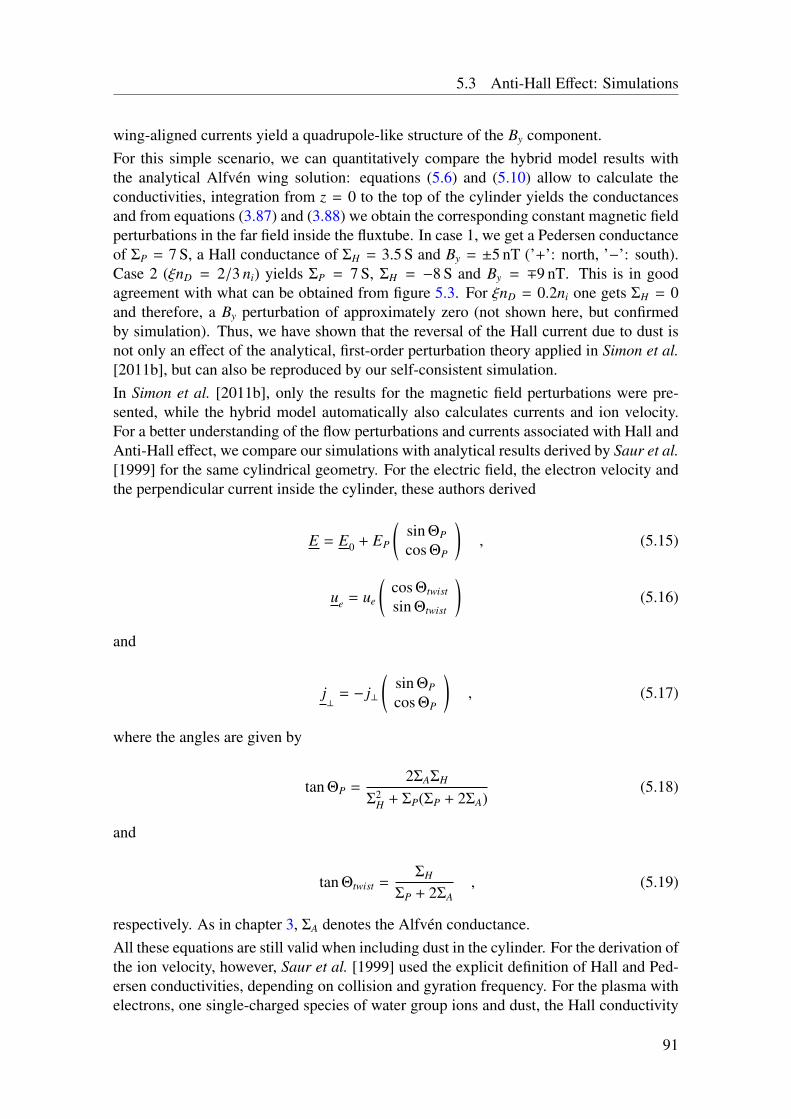
5.3 Anti-Hall Effect: Simulations
wing-aligned currents yield a quadrupole-like structure of the By component.For this simple scenario, we can quantitatively compare the hybrid model results withthe analytical Alfvén wing solution: equations (5.6) and (5.10) allow to calculate theconductivities, integration from z = 0 to the top of the cylinder yields the conductancesand from equations (3.87) and (3.88) we obtain the corresponding constant magnetic fieldperturbations in the far field inside the fluxtube. In case 1, we get a Pedersen conductanceof ΣP = 7 S, a Hall conductance of ΣH = 3.5 S and By = ±5 nT (’+’: north, ’−’: south).Case 2 (ξnD = 2/3 ni) yields ΣP = 7 S, ΣH = −8 S and By = ∓9 nT. This is in goodagreement with what can be obtained from figure 5.3. For ξnD = 0.2ni one gets ΣH = 0and therefore, a By perturbation of approximately zero (not shown here, but confirmedby simulation). Thus, we have shown that the reversal of the Hall current due to dust isnot only an effect of the analytical, first-order perturbation theory applied in Simon et al.[2011b], but can also be reproduced by our self-consistent simulation.In Simon et al. [2011b], only the results for the magnetic field perturbations were pre-sented, while the hybrid model automatically also calculates currents and ion velocity.For a better understanding of the flow perturbations and currents associated with Hall andAnti-Hall effect, we compare our simulations with analytical results derived by Saur et al.[1999] for the same cylindrical geometry. For the electric field, the electron velocity andthe perpendicular current inside the cylinder, these authors derived
E = E0 + EP
(sin ΘP
cos ΘP
), (5.15)
ue = ue
(cos Θtwist
sin Θtwist
)(5.16)
and
j⊥
= − j⊥
(sin ΘP
cos ΘP
), (5.17)
where the angles are given by
tan ΘP =2ΣAΣH
Σ2H + ΣP(ΣP + 2ΣA)
(5.18)
and
tan Θtwist =ΣH
ΣP + 2ΣA, (5.19)
respectively. As in chapter 3, ΣA denotes the Alfvén conductance.All these equations are still valid when including dust in the cylinder. For the derivation ofthe ion velocity, however, Saur et al. [1999] used the explicit definition of Hall and Ped-ersen conductivities, depending on collision and gyration frequency. For the plasma withelectrons, one single-charged species of water group ions and dust, the Hall conductivity
91
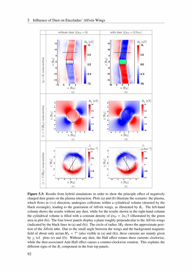
5 Influence of Dust on Enceladus’ Alfvén Wings
without dust (ξnD = 0) with dust (ξnD = 2/3ni)
(y=
0)cr
oss-
sect
ion
By [nT]
z[R
E]
x [RE ](a)
By [nT]
z[R
E]
x [RE ](b)
(z=
7.5R
E)
cros
s-se
ctio
n
x [RE ]
y[R
E]
By [nT]
(c)
x [RE ]
y[R
E]
By [nT]
(d)
(z=
7.5R
E)
cros
s-se
ctio
n
jz[µAm−2]
x [RE ]
y[R
E]
(e)
jz[µAm−2]
x [RE ]
y[R
E]
(f)
1Figure 5.3: Results from hybrid simulations in order to show the principle effect of negativelycharged dust grains on the plasma interaction. Plots (a) and (b) illustrate the scenario: the plasma,which flows in (+x) direction, undergoes collisions within a cylindrical volume (denoted by theblack rectangle), leading to the generation of Alfvén wings, as illustrated by By. The left-handcolumn shows the results without any dust, while for the results shown in the right-hand columnthe cylindrical volume is filled with a constant density of ξnD = 2ni/3 (illustrated by the greenarea in plot (b)). The four lower panels display a plane roughly perpendicular to the Alfvén wings(indicated by the black lines in (a) and (b)). The circle of radius 3RE shows the approximate posi-tion of the Alfvén tube. Due to the small angle between the wings and the background magneticfield of about only arctan MA = 7 (also visible in (a) and (b)), these currents are mainly givenby jz (cf. plots (e) and (f)). Without any dust, the Hall effect rotates these currents clockwise,while the dust-associated Anti-Hall effect causes a counter-clockwise rotation. This explains thedifferent signs of the By component in the four top panels.
92
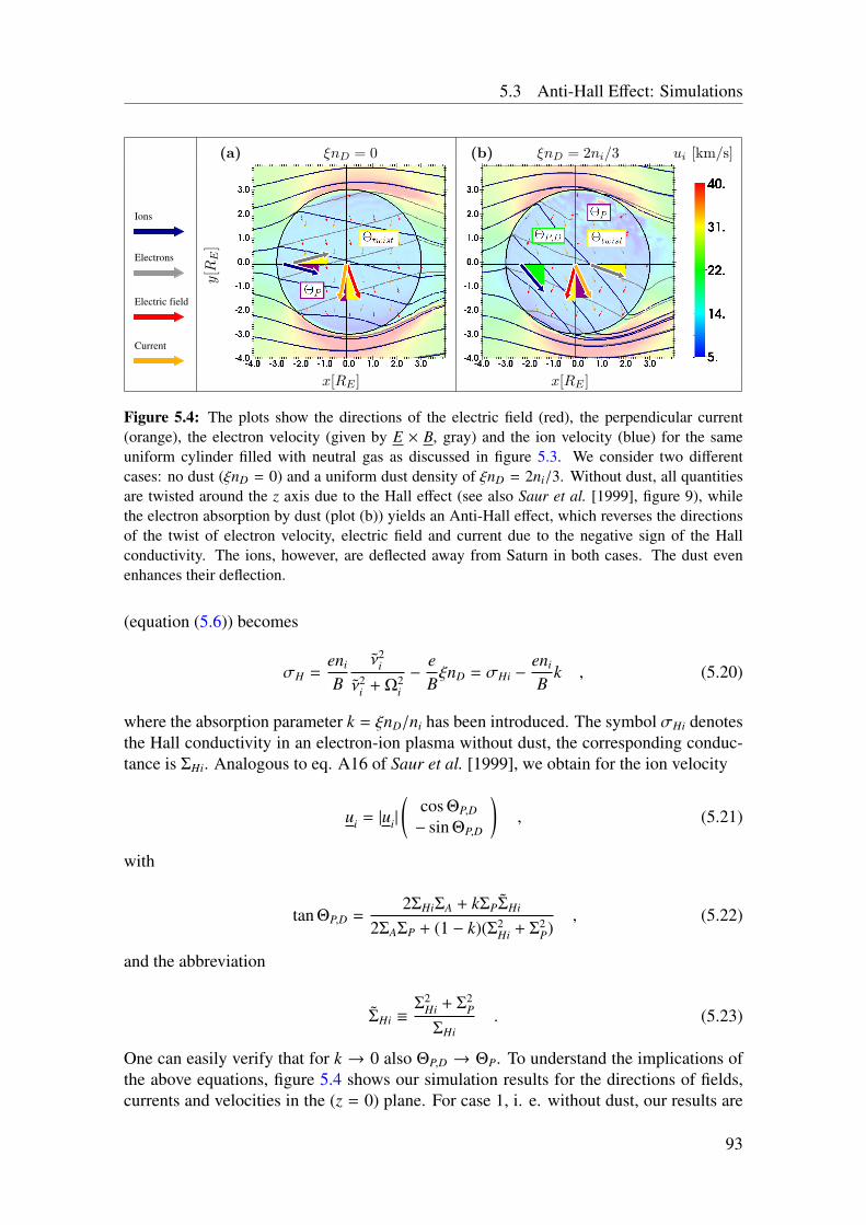
5.3 Anti-Hall Effect: Simulations
(a) ξnD = 0 (b) ξnD = 2ni/3 ui [km/s]
Current
Electric field
Electrons
Ionsy[R
E]
x[RE ] x[RE ]
Figure 5.4: The plots show the directions of the electric field (red), the perpendicular current(orange), the electron velocity (given by E × B, gray) and the ion velocity (blue) for the sameuniform cylinder filled with neutral gas as discussed in figure 5.3. We consider two differentcases: no dust (ξnD = 0) and a uniform dust density of ξnD = 2ni/3. Without dust, all quantitiesare twisted around the z axis due to the Hall effect (see also Saur et al. [1999], figure 9), whilethe electron absorption by dust (plot (b)) yields an Anti-Hall effect, which reverses the directionsof the twist of electron velocity, electric field and current due to the negative sign of the Hallconductivity. The ions, however, are deflected away from Saturn in both cases. The dust evenenhances their deflection.
(equation (5.6)) becomes
σH =eni
Bν2
i
ν2i + Ω2
i
−eBξnD = σHi −
eni
Bk , (5.20)
where the absorption parameter k = ξnD/ni has been introduced. The symbol σHi denotesthe Hall conductivity in an electron-ion plasma without dust, the corresponding conduc-tance is ΣHi. Analogous to eq. A16 of Saur et al. [1999], we obtain for the ion velocity
ui = |ui|
(cos ΘP,D
− sin ΘP,D
), (5.21)
with
tan ΘP,D =2ΣHiΣA + kΣPΣHi
2ΣAΣP + (1 − k)(Σ2Hi + Σ2
P), (5.22)
and the abbreviation
ΣHi ≡Σ2
Hi + Σ2P
ΣHi. (5.23)
One can easily verify that for k → 0 also ΘP,D → ΘP. To understand the implications ofthe above equations, figure 5.4 shows our simulation results for the directions of fields,currents and velocities in the (z = 0) plane. For case 1, i. e. without dust, our results are
93
5 Influence of Dust on Enceladus’ Alfvén Wings
shown in plot 5.4(a). One can clearly see the deflection of electric field, electron velocity,current and ion velocity with the angles ΘP and Θtwist. From equations (5.18), (5.19) weget Θtwist ≈ ΘP ≈ 13, which is in good agreement with our simulation results.The situation gets different with dust. In an electron-ion plasma without dust, a vanishingHall conductance ΣH ≈ 0 implies νi ≈ 0 and therefore no deflection of electric field, elec-tron velocity, current and ion velocity. With dust, however, the modified quasi-neutralitycondition (ni = ne + ξnD) yields ΣH ≈ 0, but ΣHi , 0 and therefore ΘPD , 0. Thus, whatwe can learn from eqs. (5.18), (5.19) and (5.22) is that only the ions should undergo adeflection. Physically this deflection is a result of the Pedersen current, where in the caseof electrons attached to dust only the ions but not the charged dust particles move withrespect to Enceladus.In case 2, the direction of rotation of electric field, current, and electron velocity reverses,since the Hall current reverses its sign. The ion flow, however, does not change its flowdirection from −y to +y, but the deflection away from Saturn gets even stronger, sinceit can be seen from eq. (5.22) that ΘP,D > ΘP for k > 0. This has the remarkableconsequence that for the ions, the dust enhances the asymmetries, while for electrons,electric field and current the direction of rotation is reversed. The angles for case 2 areΘtwist = −28, ΘP = −20 and ΘP,D = 54, which match well with figure 5.4(b).It is therefore shown that A.I.K.E.F. is able to reproduce the sign of the observed By
perturbation according to the presence of negatively charged dust, i. e. the Anti-Halleffect is successfully included in the model. The results are in quantitative agreementwith the analytical theory of the Alfvén wing. For a quantitative comparison with Cassinidata, however, a realistic model of the plume needs to be included. Hence, we extend ourprevious hybrid model of Enceladus’ plasma interaction [Kriegel et al. 2009] such that wenow include momentum loading via charge exchange as well as the electron absorptionby dust. The following problems are addressed:
• We compare Cassini magnetometer data with our simulations that include a realisticneutral plume model and negative dust.
• Based on this comparison, we estimate variations in plume activity and a possibletilt of the plume for the flybys E5 – E9 and E11.
5.4 Modeling Enceladus
The hybrid model and the A.I.K.E.F. code have already been described in chapter 4. Here,we will therefore summarize only the numerical and physical parameters which are usedfor the simulations presented in this chapter. Furthermore, the models of the neutral anddust plume are described.
5.4.1 Simulation Parameters and Geometry
As discussed in section 2.2, the magnetospheric plasma impinging on Enceladus consistsmainly of O+, OH+, H2O+ and H3O+ [Tokar et al. 2006, 2008]. To study the basic effect
94
5.4 Modeling Enceladus
of the dust on Enceladus’ Alfvén wings, however, we consider only a single species ofwater group ions (W+) with an average mass of mi = 17.5 amu. We assume that the ionsflow at the ideal corotation velocity of u0 = (26.4,0,0) km/s relative to Enceladus. Asdiscussed in section 2.2, Cassini observations show evidence for a sub-corotation of theupstream flow [Wahlund et al. 2005, 2009, Wilson et al. 2009], whereas our assumptionof ideal corotation was mainly made to improve numerical stability. However, this doesnot affect our conclusions, since we are interested in the general plasma structures andrelative variations of the plume. Assuming that all upstream ion species have roughlyequal abundances [Tokar et al. 2006], the major reactions with the neutral water moleculesof the plume yield an average rate of kαβ = kW+ = 2.2 · 10−9cm3/s (see e.g. appendix ofFleshman et al. [2010b]). A more detailed analysis of the ion neutral chemistry will bepresented in the next chapter. The electron pressure (equation (B)) includes contributionsfrom two electron populations: a warm population with kBTew=100 eV, which makes upa fraction of 0.5% of the total electron density and a cold population with kBTec = 1.35eV. The background magnetic field is approximated by a dipole field which is fitted to theunperturbed upstream field of the respective flyby. At the center of Enceladus, the field isapproximately given by B0 = (0, 0,−325 nT). The density of the upstream plasma is setindividually for each flyby according to the values listed in table 2.2. An overview aboutthe physical parameters is provided in table 5.1. Those values which are not mentionedhere in the text have been adopted from table 2.4.Photoionization and electron impact ionization are considered as ionization processes.The photoionization rate for water is νphoto = 4.4 · 10−9/s at 9.5 AU for quiet solar con-ditions [Burger et al. 2007]. This rate is kept spatially constant, since none of the flybysdiscussed here occurred in Saturn’s geometric shadow and the plume is assumed to beoptically thin. The electron impact ionization is mainly carried by the warm electronpopulation which possesses a rate coefficient of Ie = 4.5 · 10−8cm3/s [Fleshman et al.2010b]. We neglect any variations in the local ionization rate due to the energy loss of theelectrons when moving through the plume.The size of our simulation box is 20RE × 20RE × 70RE for the simulations presented inthis chapter. Because of the south-polar plume and the associated structures, Enceladusis not placed at the center of the box, but at 4/7 of the box height. We use a hierarchicalmesh that is adaptive in space but static in time, with up to three levels of refinement:L0, L1, L2. At the coarsest level (L0), the resolution is ∆L0 = 53km = 0.21RE, while it is∆L2 = 1
4∆L0 = 13km = 0.05RE in the highest level. The spatial extension of the refinementlevels is illustrated by the plots of our mesh in figures 5.5(a) and 5.5(d). Due to limitedcomputational resources, we were not able to perform every simulation with the highestresolution, but only the final (best fit) runs. All other runs are carried out using a meshwith only two levels of refinement (L0, L1), since we did not notice a remarkable depen-dency of our results on the grid resolution. The ions and the dust are represented by 100macroparticles per species, yielding a total of more than one billion macroparticles in thesimulation. The physical and numerical parameters are summarized in table 5.1. Furthernumerical aspects like boundary conditions and smoothing are described in sections 4.5and 4.4.
95
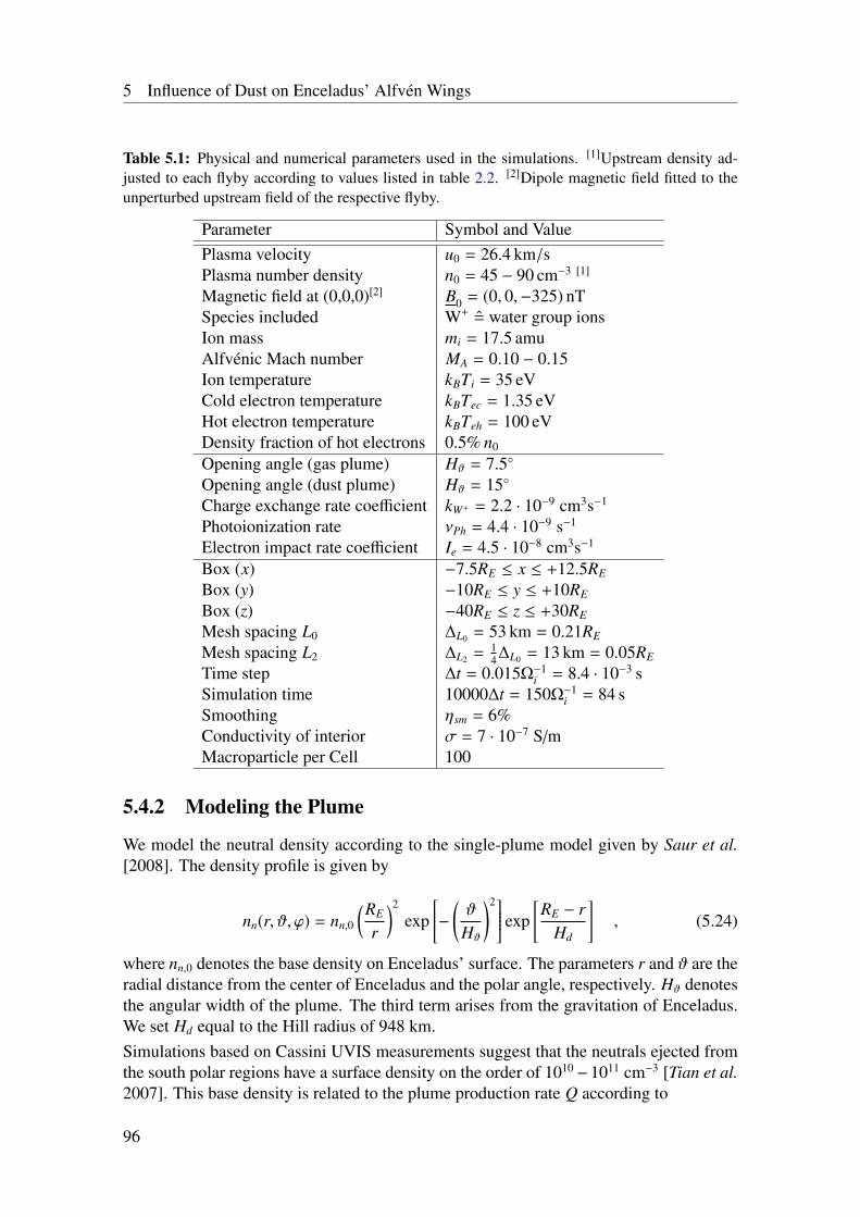
5 Influence of Dust on Enceladus’ Alfvén Wings
Table 5.1: Physical and numerical parameters used in the simulations. [1]Upstream density ad-justed to each flyby according to values listed in table 2.2. [2]Dipole magnetic field fitted to theunperturbed upstream field of the respective flyby.
Parameter Symbol and ValuePlasma velocity u0 = 26.4 km/sPlasma number density n0 = 45 − 90 cm−3 [1]
Magnetic field at (0,0,0)[2] B0 = (0, 0,−325) nTSpecies included W+ = water group ionsIon mass mi = 17.5 amuAlfvénic Mach number MA = 0.10 − 0.15Ion temperature kBTi = 35 eVCold electron temperature kBTec = 1.35 eVHot electron temperature kBTeh = 100 eVDensity fraction of hot electrons 0.5% n0
Opening angle (gas plume) Hϑ = 7.5
Opening angle (dust plume) Hϑ = 15
Charge exchange rate coefficient kW+ = 2.2 · 10−9 cm3s−1
Photoionization rate νPh = 4.4 · 10−9 s−1
Electron impact rate coefficient Ie = 4.5 · 10−8 cm3s−1
Box (x) −7.5RE ≤ x ≤ +12.5RE
Box (y) −10RE ≤ y ≤ +10RE
Box (z) −40RE ≤ z ≤ +30RE
Mesh spacing L0 ∆L0 = 53 km = 0.21RE
Mesh spacing L2 ∆L2 = 14∆L0 = 13 km = 0.05RE
Time step ∆t = 0.015Ω−1i = 8.4 · 10−3 s
Simulation time 10000∆t = 150Ω−1i = 84 s
Smoothing ηsm = 6%Conductivity of interior σ = 7 · 10−7 S/mMacroparticle per Cell 100
5.4.2 Modeling the Plume
We model the neutral density according to the single-plume model given by Saur et al.[2008]. The density profile is given by
nn(r, ϑ, ϕ) = nn,0
(RE
r
)2
exp− (
ϑ
Hϑ
)2 exp[RE − r
Hd
], (5.24)
where nn,0 denotes the base density on Enceladus’ surface. The parameters r and ϑ are theradial distance from the center of Enceladus and the polar angle, respectively. Hϑ denotesthe angular width of the plume. The third term arises from the gravitation of Enceladus.We set Hd equal to the Hill radius of 948 km.Simulations based on Cassini UVIS measurements suggest that the neutrals ejected fromthe south polar regions have a surface density on the order of 1010 − 1011 cm−3 [Tian et al.2007]. This base density is related to the plume production rate Q according to
96
5.4 Modeling Enceladus
nn,0 =Q
AunR2E
, (5.25)
where A = 0.054 is an integration constant due to the opening angle of the plume (see Jiaet al. [2010c]). Assuming a neutral speed of un = 1 km/s, a surface density of 1010 cm−3
corresponds to a plume production rate of 3 · 1028 H2O/s.Measurements and simulations indicate a variation in the activities of the jets [Saur et al.2008, Kriegel et al. 2009, Teolis et al. 2010, Tenishev et al. 2010, Smith et al. 2010].Therefore, nn,0 is treated as a free parameter to model the source strength for the individualflybys. We vary nn,0 between different simulation runs in steps of 1 · 1010 cm−3.Spitale and Porco [2007] showed that the plume consists of at least eight jets. However,Saur et al. [2008] showed that a multi-plume model might not be necessary to reproduceMAG data. The effect of the single jets on the global shape of the plume is mainlygiven by variations in the location of active regions, which may yield a global tilt ofthe plume. For each flyby, we therefore tested different tilts of the plume in order toachieve best possible agreement with MAG data. In the ENIS system, the symmetry axisof the plume has the direction (cosϕ0 sinϑ0, sinϕ0 sinϑ0, cosϑ0), with ϕ0 ∈ [0; 360] andϑ0 ∈ [90; 180]. These angles correspond to planetographic latitude (Lat.) and longitude(Lon.) on Enceladus’ surface as follows: 90 − ϑ0 = Lat.() and the correlation betweenϕ0 and Lon. is given by (0 = 90W, 90 = 0W, 180 = 270W, 270 = 180W).Please note that the angle ϕ0 is measured in counter-clockwise direction (with respect tothe ENIS system), whereas the value of Lon. increases when moving clockwise aroundEnceladus. Since these additional parameters strongly increase the number of necessarysimulations, we at first checked, if a tilt of the symmetry axis towards planetary latitudesof −80 along the ±x and ±y axis yielded any notable improvement when comparing ourresults with Cassini MAG data. If that was the case, we further varied the latitude in stepsof ϑ0 = 5 and the longitude in steps of ϕ0 = 22.5 to find the optimal set of parameters.From UVIS observations during a star occultation on 24 October 2007, Hansen et al.[2008] obtained a Mach number of the gas of about M = 1.5, which is in agreementwith simulations [Tian et al. 2007, Smith et al. 2010, Tenishev et al. 2010]. Assuminga gas temperature of 150 K (that is a thermal speed of vth = 455 m/s), this yields anoutgassing velocity of un = 680 m/s. More recent data suggest a even higher velocityof M = 4 [Hansen et al. 2010]. A Mach number in the range of 1.5 – 4 corresponds toopening angles of the individual jets of arctan(vth/un) = 30 − 15. However, as we usea single-plume model, the opening angle Hϑ includes both, ejection speed and locationof the vents. We found that our simulations yield a considerably better agreement with amore confined plume and therefore set Hϑ = 7.5 (see also section 5.5.2). With regard tothe dynamics of the ions, however, we found that a neutral velocity on the order of 1 km/sdoes not have a noteworthy influence on the outcome of the simulation. For simplicity,we therefore neglect the neutrals’ velocity in the ionization processes, i.e. the newlygenerated ions start with initial velocity zero.
97
5 Influence of Dust on Enceladus’ Alfvén Wings
5.4.3 Dusty Plasma Parameters
According to Farrell et al. [2010] and Shafiq et al. [2011], the charged submicron-sizeddust grains in the Enceladus plume may be considered an additional plasma constituent,since the inter-grain distance for dust densities of nD ≥ 10−1 cm−3 is smaller than theeffective dusty plasma Debye length of λE f f ∼ 1 m. Assuming spherical grains with amass density of ρ = 103 kg/m3 (water ice) and an average number of ξ = 50 electronsfor a grain size of 0.03 µm and ξ = 8000 for a grain size of 1 µm, the charge-to-massratio ranges from qD/mD = 3 · 10−1 C/kg to qD/mD = 7 · 101 C/kg [Shafiq et al. 2011].Therefore, we consider the charged dust as an additional plasma species with a charge-to-mass ratio of qD/mD = 5.5 C/kg = 10−6 qW+/mW+ . Due to this small charge-to-mass ratio,this averaged dust species does practically not move during the simulation runtime, whichis on the order of a few minutes. We would like to note that this would still be true fornanometer-sized grains with a significantly larger charge-to-mass ratio of qD,nm/mD,nm ∼
10−4 qW+/mW+ , since the accelerating electric field is strongly reduced within the centerof the plume (see section 5.5). Moreover, the resulting dust charge density can also beinterpreted to include a fraction of positively charged grains as reported by Jones et al.[2009], because only the total dust charge density is taken into account by our simulations.The presence of positively charged grains would then just mean that the density of thenegative grains is even larger.The source strength of the dusty part of the plume is characterized analogously to the gasplume by the density ξnD,0 of charged dust at the south pole, which is varied in steps of50 cm−3. We would like to note that we only describe a stationary density profile of thecharged dust in our model, while a self-consistent model of the electron absorption isout of the scope of this paper and will be addressed in chapter 6. Some implications ofthis approximation are also discussed in section 4.3 in Simon et al. [2011b]. The spatialdensity profile of the dust is similar to the neutral density profile (eq. (5.24)). However,due to the ejection speeds of the dust grains being comparable to the escape velocity ofEnceladus, the influence of gravitation and inertia forces is larger for the dust grains thanfor the gas, leading to complicated trajectories around Enceladus [Kempf et al. 2010]. Weaccount for that by setting Hϑ = 15 for the dust. Moreover, the charging time dependson grain size and the ambient plasma conditions. Therefore, the spatial profile of the dustcharge density in the plume may be different from the profile of the dust number density.We find that our results are in better agreement with Cassini MAG data, if we replace thegeometric r−2 decrease (see eq. (5.24)) by r−1. The resulting profile does not claim to bea quantitatively realistic image of the charged dust population at Enceladus. This wouldrequire a much more sophisticated model of the grain-size-distribution of the dust, thedust motion in the three-body-problem and the dust charging process, which is presentedin chapter 6.
5.5 Results for Selected Enceladus Flybys
In order to understand the magnetic field measurements and model calculations alongCassini’s 1D-trajectories, we present the results of our 3D simulations together with 1Dcomparisons between model and observations. We show that considering the electron
98
5.5 Results for Selected Enceladus Flybys
absorption is necessary to quantitatively explain the observations. However, before we canunderstand the magnetic field structures, we have to consider the corresponding structuresof plasma density and velocity.Since upstream and plume parameters are different for each flyby discussed here, wearbitrarily choose the E9 best fit case with an upstream density of n0 = 75 cm−3 and abase density of nn,0 = 6 ·1010cm−3 for all color plots shown in this section. The simulationincluding dust has an additional dust base density of ξnD,0 = 5.5 · 102 cm−3.
5.5.1 Density and Velocity
Figure 5.5 displays the densities of ions and charged dust in the (y = 0) and (z = −4RE)planes. Plots 5.5(b) and 5.5(e) visualize the gas plume as the region where the ion densityis enhanced due to the creation of new ions by electron impacts and photoionization (massloading). Near the south pole, the ion density is about an order of magnitude larger thanupstream. The slightly enhanced density downstream of the plume results from pick-upof the newly created ions [Kriegel et al. 2009]. The dust charge density ξnD (plots 5.5(c)and 5.5(e)) has a maximum of ξnD > 100 cm−3 near the south pole and assumes a valueof about ξnD = 50 cm−3 at z = −4RE. Thus, the dropout in the electron density due toelectron absorption by dust, which is required by our model to achieve agreement withMAG data (see next sections), is on the order of 10%− 20% in the center of the plume. Itis therefore possible to have a noteable difference in electron and ion densities while bothare larger than the background density. This finding is in agreement with results fromRPWS presented by Shafiq et al. [2011]. Since we can only provide dust charge densities,it is not easily possible to compare our results with dust measurements (for example byCDA). In order to relate our model densities of the charged dust to number densities,one would need to consider the number of electrons on grains of different sizes and thegrain-size distribution of the dust which will be done in chapter 6.Ion velocity and electric field are presented in the lower row of figure 5.5. In plot 5.5(g),one can see the deflection of the ion flow in (−y) direction (away from Saturn), as dis-cussed in section 5.3. The twist of the electric field in (−x) direction in plot 5.5(h) resultsfrom the Anti-Hall effect. As can be seen from plots 5.5(g) and 5.5(h), the pickup tailand the associated decrease in the electric field strength are essentially confined to the(|y| < 1RE)-region, i.e. the tail exhibits a two-dimensional shape. This finding is in agree-ment with our previous hybrid simulation results where it has been shown that the smallgyroradii of the pick-up ions (on the order of 10 km) prevent the tail from a significantexpansion in y direction [Kriegel et al. 2009]. Within the plume, ion velocity and electricfield decrease to approximately zero, in agreement with observations of flow stagnationby CAPS [Tokar et al. 2009]. To further illustrate the effect of flow stagnation, figure5.5(i) displays the ion velocity in the (z = −4RE) plane along the corotation axis (y = 0line): the ion velocity decreases sharply below 1 km/s from x = −1RE to x = 0.5RE,before it assumes a value of ui = 17 km/s = 60% u0 in the pick-up tail.
99
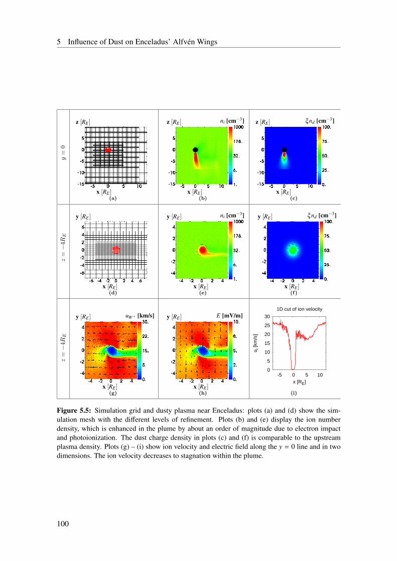
5 Influence of Dust on Enceladus’ Alfvén Wings
y=
0
x [RE ]
z [RE ]
1
(a)x [RE ]
z [RE ] ni [cm−3]
1
(b)x [RE ]
z [RE ] ξ nd [cm−3]
1
(c)
z=−
4RE
x [RE ]
y [RE ]
1
(d)x [RE ]
y [RE ] ni [cm−3]
1
(e)x [RE ]
y [RE ] ξ nd [cm−3]
1
(f)
z=−
4RE
x [RE ]
y [RE ] uW+ [km/s]
1
(g)x [RE ]
y [RE ] E [mV/m]
1
(h)
0
5
10
15
20
25
30
-5 0 5 10
u i [k
m/s
]
x [RE]
1D cut of ion velocity
(i)
Figure 5.5: Simulation grid and dusty plasma near Enceladus: plots (a) and (d) show the sim-ulation mesh with the different levels of refinement. Plots (b) and (e) display the ion numberdensity, which is enhanced in the plume by about an order of magnitude due to electron impactand photoionization. The dust charge density in plots (c) and (f) is comparable to the upstreamplasma density. Plots (g) – (i) show ion velocity and electric field along the y = 0 line and in twodimensions. The ion velocity decreases to stagnation within the plume.
100
5.5 Results for Selected Enceladus Flybys
5.5.2 Magnetic Field: E5 and E6
All Enceladus flybys in 2008 had trajectories basically in the (x, z) plane. For a betterunderstanding of the perturbations visible in the MAG data, figure 5.6 shows the resultsfor the components of the magnetic field in that plane. For clarity, the color plots onlyshow the magnetic field perturbations (∆Bx,∆By,∆Bz), the background field has beensubtracted by fitting a dipole field. The black lines represent the projections of Cassini’strajectories during E5 and E6 on the (x, z) plane. The first row shows the results for a puregas plume without dust. In plot 5.6(a), the Alfvén wing can clearly be seen in the ∆Bx
component. ∆By (plot 5.6(b)) assumes positive and negative signs in both, the northernand the southern wing, which results from the clockwise rotation of the quadrupole-likestructure of ∆By due to the Hall effect. The positive sign of ∆By in the center of thenorthern wing as well as the negative sign in the center of the southern wing are consistentwith the results for the test scenario (see figure 5.3). We would like to note that an idealMHD model (i.e. without Hall effect) would yield ∆By ≈ 0 at y = 0. The ∆Bz componentin plot (c) assumes a negative value in the magnetic pile-up region in front of the plumeand a positive value at the downstream side (since it is Bz < 0 for the background field).These structures have already been described in detail in our previous study [Kriegel et al.2009] as well as by Jia et al. [2010c].The middle row of figure 5.6 (plots (d) – (f)) shows the results of a simulation with dustincluded. As expected, the ∆By component inside the Alfvén fluxtube has reversed itssign. On the other hand, no modification of ∆Bx is visible. In section 5.7, we will discussin which regions the condition for the occurrence of the Anti-Hall effect (inequality (5.8))is fulfilled . The most important result, especially with respect to the work presented inSimon et al. [2011b], is that the reversal of ∆By due to electron absorption by dust alsooccurs for a more realistic, inhomogeneous plume model.In contrast to what is claimed in recent literature [Jia et al. 2010a,b,c], it is therefore notnecessary to account for the large-scale, centrifugally driven dynamics of the flux tubesin Saturn’s magnetosphere in order to understand magnetic field observations within theEnceladus plume. However, for a realistic description of Enceladus’ magnetospheric in-teraction, (at least) three plasma species need to be taken into account: electrons, wa-ter group ions, and the dust grains, where the dust grains include a wide distribution ofcharge-to-mass ratios.We would also like to point out that our results show that the northern wing (negative∆Bx) does not begin at Enceladus’ south pole, but about 2 RE below. Thus, our simulationconfirms that the draping center is shifted about 2 RE downward from the south pole, inagreement with the findings of Khurana et al. [2007] for E0 – E2. It is remarkable thatour simulation succeeds in reproducing this aspect of the interaction without reducingthe neutral density near the south pole to account for a reduced ionization efficiency inthat region, as proposed by Jia et al. [2010c]. By comparing the ∆Bz components inplots 5.6(c) and 5.6(f), one can see that the region of magnetic field decrease is shifteddownward, if dust is considered.A quantitative comparison between MAG data from E5 and E6 and simulation results isprovided in the bottom row of figure 5.6. MAG data are colored in black, the other colorsindicate different simulation setups: no dust (green), with dust (blue) and the best fit with
101
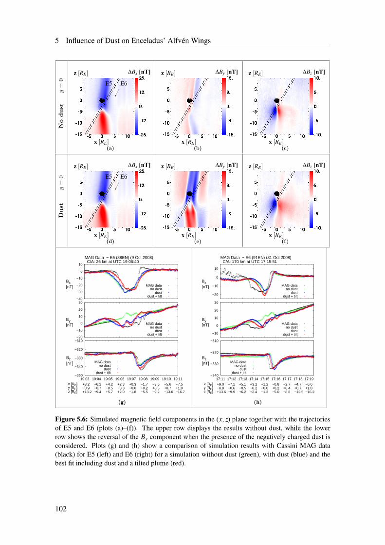
5 Influence of Dust on Enceladus’ Alfvén Wings
No
dust
y=
0
E6E5
x [RE ]
z [RE ] ∆Bx [nT]
1
(a)x [RE ]
z [RE ] ∆By [nT]
1
(b)x [RE ]
z [RE ] ∆Bz [nT]
1
(c)
Dust
y=
0
E6E5
x [RE ]
z [RE ] ∆Bx [nT]
1
(d)x [RE ]
z [RE ] ∆By [nT]
1
(e)x [RE ]
z [RE ] ∆Bz [nT]
1
(f)
−40
−30
−20
−10
0
10
19:03 19:04 19:05 19:06 19:07 19:08 19:09 19:10 19:11
MAG Data − E5 (88EN) (9 Oct 2008) C/A: 26 km at UTC 19:06:40
Bx [nT] MAG data
no dustdust
dust + tilt
−20
−10
0
10
20
30
19:03 19:04 19:05 19:06 19:07 19:08 19:09 19:10 19:11
By [nT] MAG data
no dustdust
dust + tilt
−350
−340
−330
−320
−310
19:03 19:04 19:05 19:06 19:07 19:08 19:09 19:10 19:11x [RE]y [RE]z [RE]
+8.2−0.9+13.2
+6.2−0.7+9.4
+4.2−0.5+5.7
+2.3−0.3+2.0
+0.3−0.0−1.8
−1.7+0.2−5.5
−3.6+0.5−9.2
−5.6+0.7−13.0
−7.5+1.0−16.7
Bz [nT] MAG data
no dustdust
dust + tilt
(g)
−20
−10
0
10
17:11 17:12 17:13 17:14 17:15 17:16 17:17 17:18 17:19
MAG Data − E6 (91EN) (31 Oct 2008) C/A: 170 km at UTC 17:15:51
Bx [nT] MAG data
no dustdust
dust + tilt
−10
0
10
20
30
17:11 17:12 17:13 17:14 17:15 17:16 17:17 17:18 17:19
By [nT] MAG data
no dustdust
dust + tilt
−340
−330
−320
−310
17:11 17:12 17:13 17:14 17:15 17:16 17:17 17:18 17:19x [RE]y [RE]z [RE]
+9.0−0.8+13.6
+7.1−0.6+9.9
+5.1−0.5+6.2
+3.2−0.2+2.4
+1.2−0.0−1.3
−0.8+0.2−5.0
−2.7+0.4−8.8
−4.7+0.7−12.5
−6.6+1.0−16.2
Bz [nT] MAG data
no dustdust
dust + tilt
(h)
Figure 5.6: Simulated magnetic field components in the (x, z) plane together with the trajectoriesof E5 and E6 (plots (a)–(f)). The upper row displays the results without dust, while the lowerrow shows the reversal of the By component when the presence of the negatively charged dust isconsidered. Plots (g) and (h) show a comparison of simulation results with Cassini MAG data(black) for E5 (left) and E6 (right) for a simulation without dust (green), with dust (blue) and thebest fit including dust and a tilted plume (red).
102
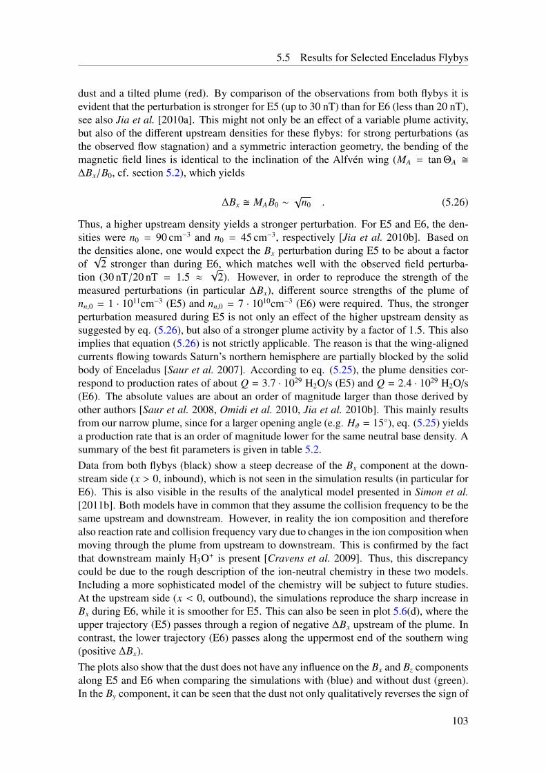
5.5 Results for Selected Enceladus Flybys
dust and a tilted plume (red). By comparison of the observations from both flybys it isevident that the perturbation is stronger for E5 (up to 30 nT) than for E6 (less than 20 nT),see also Jia et al. [2010a]. This might not only be an effect of a variable plume activity,but also of the different upstream densities for these flybys: for strong perturbations (asthe observed flow stagnation) and a symmetric interaction geometry, the bending of themagnetic field lines is identical to the inclination of the Alfvén wing (MA = tan ΘA ∆Bx/B0, cf. section 5.2), which yields
∆Bx MAB0 ∼√
n0 . (5.26)
Thus, a higher upstream density yields a stronger perturbation. For E5 and E6, the den-sities were n0 = 90 cm−3 and n0 = 45 cm−3, respectively [Jia et al. 2010b]. Based onthe densities alone, one would expect the Bx perturbation during E5 to be about a factorof√
2 stronger than during E6, which matches well with the observed field perturba-tion (30 nT/20 nT = 1.5 ≈
√2). However, in order to reproduce the strength of the
measured perturbations (in particular ∆Bx), different source strengths of the plume ofnn,0 = 1 · 1011cm−3 (E5) and nn,0 = 7 · 1010cm−3 (E6) were required. Thus, the strongerperturbation measured during E5 is not only an effect of the higher upstream density assuggested by eq. (5.26), but also of a stronger plume activity by a factor of 1.5. This alsoimplies that equation (5.26) is not strictly applicable. The reason is that the wing-alignedcurrents flowing towards Saturn’s northern hemisphere are partially blocked by the solidbody of Enceladus [Saur et al. 2007]. According to eq. (5.25), the plume densities cor-respond to production rates of about Q = 3.7 · 1029 H2O/s (E5) and Q = 2.4 · 1029 H2O/s(E6). The absolute values are about an order of magnitude larger than those derived byother authors [Saur et al. 2008, Omidi et al. 2010, Jia et al. 2010b]. This mainly resultsfrom our narrow plume, since for a larger opening angle (e.g. Hϑ = 15), eq. (5.25) yieldsa production rate that is an order of magnitude lower for the same neutral base density. Asummary of the best fit parameters is given in table 5.2.Data from both flybys (black) show a steep decrease of the Bx component at the down-stream side (x > 0, inbound), which is not seen in the simulation results (in particular forE6). This is also visible in the results of the analytical model presented in Simon et al.[2011b]. Both models have in common that they assume the collision frequency to be thesame upstream and downstream. However, in reality the ion composition and thereforealso reaction rate and collision frequency vary due to changes in the ion composition whenmoving through the plume from upstream to downstream. This is confirmed by the factthat downstream mainly H3O+ is present [Cravens et al. 2009]. Thus, this discrepancycould be due to the rough description of the ion-neutral chemistry in these two models.Including a more sophisticated model of the chemistry will be subject to future studies.At the upstream side (x < 0, outbound), the simulations reproduce the sharp increase inBx during E6, while it is smoother for E5. This can also be seen in plot 5.6(d), where theupper trajectory (E5) passes through a region of negative ∆Bx upstream of the plume. Incontrast, the lower trajectory (E6) passes along the uppermost end of the southern wing(positive ∆Bx).The plots also show that the dust does not have any influence on the Bx and Bz componentsalong E5 and E6 when comparing the simulations with (blue) and without dust (green).In the By component, it can be seen that the dust not only qualitatively reverses the sign of
103
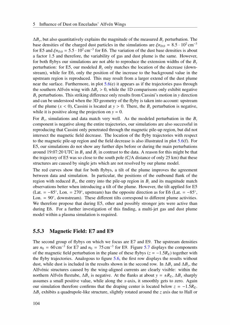
5 Influence of Dust on Enceladus’ Alfvén Wings
∆By, but also quantitatively explains the magnitude of the measured By perturbation. Thebase densities of the charged dust particles in the simulations are ξnD,0 = 8.5 · 102 cm−3
for E5 and ξnD,0 = 5.5 · 102 cm−3 for E6. The variation of the dust base densities is abouta factor 1.5 and therefore, the variability of gas and dust plume is the same. However,for both flybys our simulations are not able to reproduce the extension widths of the By
perturbation: for E5, our modeled By only matches the location of the decrease (down-stream), while for E6, only the position of the increase to the background value in theupstream region is reproduced. This may result from a larger extend of the dust plumenear the surface. Furthermore, in plot 5.6(e) it appears as if the trajectories pass throughthe southern Alfvén wing with ∆By > 0, while the 1D comparisons only exhibit negativeBy perturbations. This striking difference only results from Cassini’s motion in y directionand can be understood when the 3D geometry of the flyby is taken into account: upstreamof the plume (x < 0), Cassini is located at y > 0. There, the By perturbation is negative,while it is positive along the projection on y = 0.For Bz, simulations and data match very well. As the modeled perturbation in the Bz
component is negative along the entire trajectories, our simulations are also successful inreproducing that Cassini only penetrated through the magnetic pile-up region, but did notintersect the magnetic field decrease. The location of the flyby trajectories with respectto the magnetic pile-up region and the field decrease is also illustrated in plot 5.6(f). ForE5, our simulations do not show any further dips before or during the main perturbationsaround 19:07:20 UTC in Bx and Bz in contrast to the data. A reason for this might be thatthe trajectory of E5 was so close to the south pole (C/A distance of only 25 km) that thesestructures are caused by single jets which are not resolved by our plume model.The red curves show that for both flybys, a tilt of the plume improves the agreementbetween data and simulation. In particular, the positions of the outbound flank of theregion with reduced Bx, the entry into the pile-up region in Bz and its magnitude matchobservations better when introducing a tilt of the plume. However, the tilt applied for E5(Lat. = −85, Lon. = 270, upstream) has the opposite direction as for E6 (Lat. = −85,Lon. = 90, downstream). These different tilts correspond to different plume activities.We therefore propose that during E5, other and possibly stronger jets were active thanduring E6. For a further investigation of this finding, a multi-jet gas and dust plumemodel within a plasma simulation is required.
5.5.3 Magnetic Field: E7 and E9
The second group of flybys on which we focus are E7 and E9. The upstream densitiesare n0 = 60 cm−3 for E7 and n0 = 75 cm−3 for E9. Figure 5.7 displays the componentsof the magnetic field perturbation in the plane of these flybys (z = −1.5RE) together withthe flyby trajectories. Analogous to figure 5.6, the first row displays the results withoutdust, while dust is included in the results shown in the second row. In ∆Bx and ∆By, theAlfvénic structures caused by the wing-aligned currents are clearly visible: within thenorthern Alfvén fluxtube, ∆Bx is negative. At the flanks at about y = ±RE, ∆Bx sharplyassumes a small positive value, while along the x-axis, it smoothly gets to zero. Againour simulation therefore confirms that the draping center is located below z = −1.5RE.∆By exhibits a quadrupole-like structure, slightly rotated around the z axis due to Hall or
104
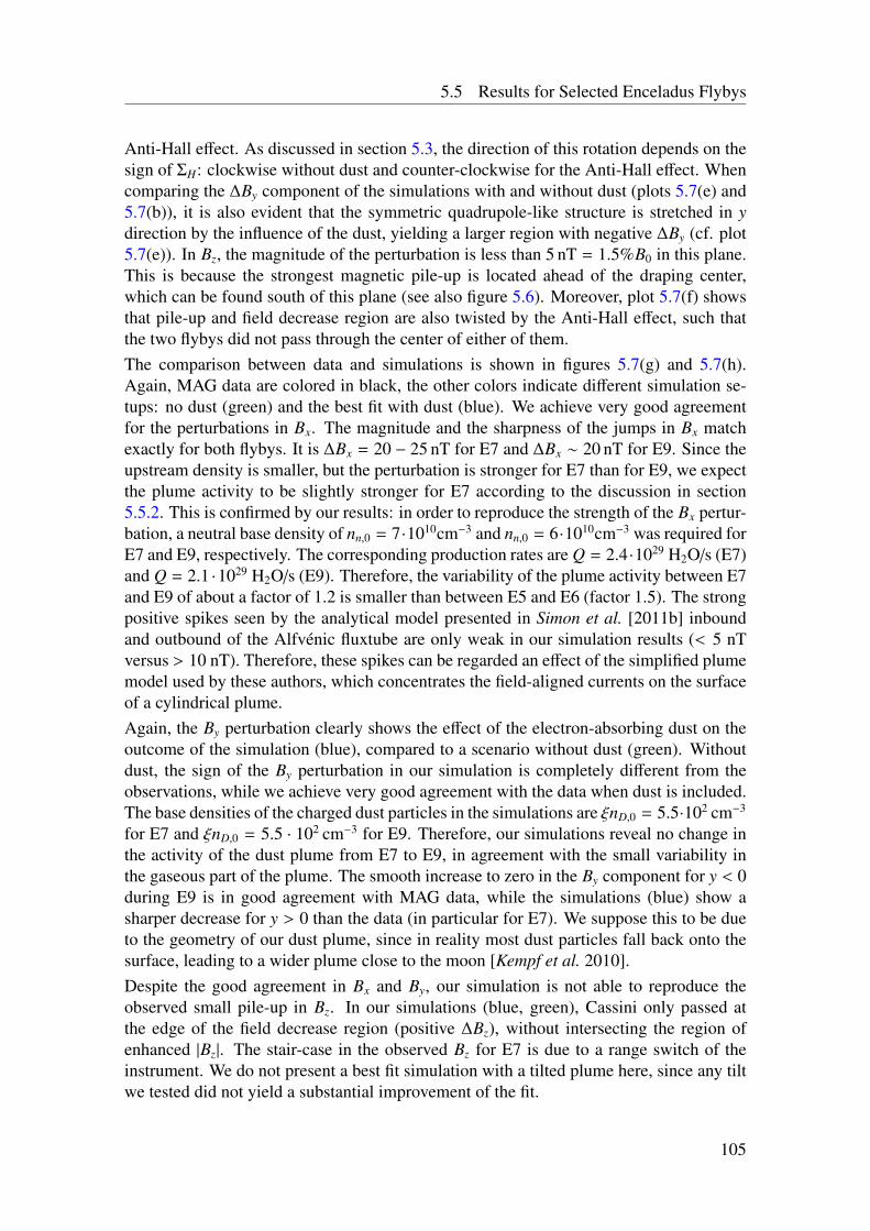
5.5 Results for Selected Enceladus Flybys
Anti-Hall effect. As discussed in section 5.3, the direction of this rotation depends on thesign of ΣH: clockwise without dust and counter-clockwise for the Anti-Hall effect. Whencomparing the ∆By component of the simulations with and without dust (plots 5.7(e) and5.7(b)), it is also evident that the symmetric quadrupole-like structure is stretched in ydirection by the influence of the dust, yielding a larger region with negative ∆By (cf. plot5.7(e)). In Bz, the magnitude of the perturbation is less than 5 nT = 1.5%B0 in this plane.This is because the strongest magnetic pile-up is located ahead of the draping center,which can be found south of this plane (see also figure 5.6). Moreover, plot 5.7(f) showsthat pile-up and field decrease region are also twisted by the Anti-Hall effect, such thatthe two flybys did not pass through the center of either of them.The comparison between data and simulations is shown in figures 5.7(g) and 5.7(h).Again, MAG data are colored in black, the other colors indicate different simulation se-tups: no dust (green) and the best fit with dust (blue). We achieve very good agreementfor the perturbations in Bx. The magnitude and the sharpness of the jumps in Bx matchexactly for both flybys. It is ∆Bx = 20 − 25 nT for E7 and ∆Bx ∼ 20 nT for E9. Since theupstream density is smaller, but the perturbation is stronger for E7 than for E9, we expectthe plume activity to be slightly stronger for E7 according to the discussion in section5.5.2. This is confirmed by our results: in order to reproduce the strength of the Bx pertur-bation, a neutral base density of nn,0 = 7·1010cm−3 and nn,0 = 6·1010cm−3 was required forE7 and E9, respectively. The corresponding production rates are Q = 2.4·1029 H2O/s (E7)and Q = 2.1 ·1029 H2O/s (E9). Therefore, the variability of the plume activity between E7and E9 of about a factor of 1.2 is smaller than between E5 and E6 (factor 1.5). The strongpositive spikes seen by the analytical model presented in Simon et al. [2011b] inboundand outbound of the Alfvénic fluxtube are only weak in our simulation results (< 5 nTversus > 10 nT). Therefore, these spikes can be regarded an effect of the simplified plumemodel used by these authors, which concentrates the field-aligned currents on the surfaceof a cylindrical plume.Again, the By perturbation clearly shows the effect of the electron-absorbing dust on theoutcome of the simulation (blue), compared to a scenario without dust (green). Withoutdust, the sign of the By perturbation in our simulation is completely different from theobservations, while we achieve very good agreement with the data when dust is included.The base densities of the charged dust particles in the simulations are ξnD,0 = 5.5·102 cm−3
for E7 and ξnD,0 = 5.5 · 102 cm−3 for E9. Therefore, our simulations reveal no change inthe activity of the dust plume from E7 to E9, in agreement with the small variability inthe gaseous part of the plume. The smooth increase to zero in the By component for y < 0during E9 is in good agreement with MAG data, while the simulations (blue) show asharper decrease for y > 0 than the data (in particular for E7). We suppose this to be dueto the geometry of our dust plume, since in reality most dust particles fall back onto thesurface, leading to a wider plume close to the moon [Kempf et al. 2010].Despite the good agreement in Bx and By, our simulation is not able to reproduce theobserved small pile-up in Bz. In our simulations (blue, green), Cassini only passed atthe edge of the field decrease region (positive ∆Bz), without intersecting the region ofenhanced |Bz|. The stair-case in the observed Bz for E7 is due to a range switch of theinstrument. We do not present a best fit simulation with a tilted plume here, since any tiltwe tested did not yield a substantial improvement of the fit.
105
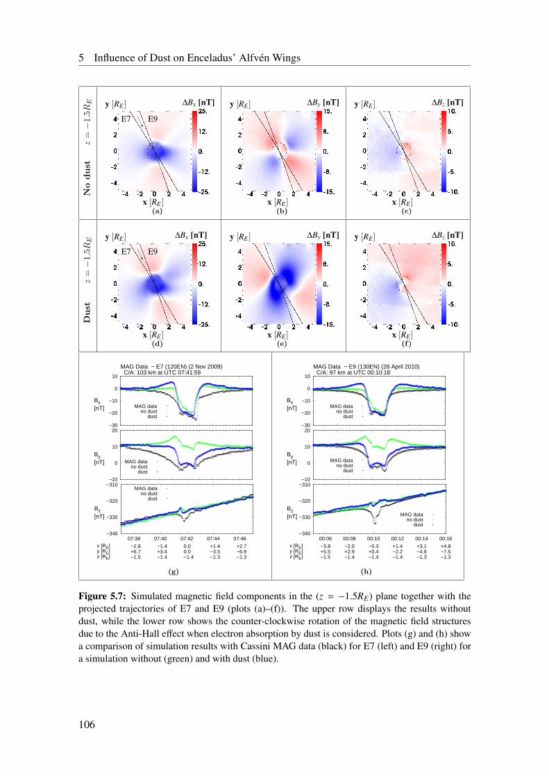
5 Influence of Dust on Enceladus’ Alfvén Wings
No
dust
z=−
1.5R
E
AAU
E7 E9
x [RE ]
y [RE ] ∆Bx [nT]
1
(a)x [RE ]
y [RE ] ∆By [nT]
1
(b)x [RE ]
y [RE ] ∆Bz [nT]
1
(c)
Dust
z=−
1.5R
E
AAU
E7 E9
x [RE ]
y [RE ] ∆Bx [nT]
1
(d)x [RE ]
y [RE ] ∆By [nT]
1
(e)x [RE ]
y [RE ] ∆Bz [nT]
1
(f)
−30
−20
−10
0
10
07:37 07:38 07:39 07:40 07:41 07:42 07:43 07:44 07:45 07:46 07:47
MAG Data − E7 (120EN) (2 Nov 2009) C/A: 103 km at UTC 07:41:59
Bx [nT] MAG data
no dustdust
−10
0
10
20
07:37 07:38 07:39 07:40 07:41 07:42 07:43 07:44 07:45 07:46 07:47
By [nT] MAG data
no dustdust
−340
−330
−320
−310
07:38 07:40 07:42 07:44 07:46x [RE]y [RE]z [RE]
−2.8+6.7−1.5
−1.4+3.4−1.4
0.00.0−1.4
+1.4−3.5−1.3
+2.7−6.9−1.3
Bz [nT]
MAG datano dust
dust
(g)
−30
−20
−10
0
10
00:05 00:06 00:07 00:08 00:09 00:10 00:11 00:12 00:13 00:14 00:15 00:16
MAG Data − E9 (130EN) (28 April 2010) C/A: 97 km at UTC 00:10:18
Bx [nT] MAG data
no dustdust
−10
0
10
20
00:05 00:06 00:07 00:08 00:09 00:10 00:11 00:12 00:13 00:14 00:15 00:16
By [nT] MAG data
no dustdust
−340
−330
−320
−310
00:06 00:08 00:10 00:12 00:14 00:16x [RE]y [RE]z [RE]
−3.8+5.5−1.5
−2.0+2.9−1.4
−0.3+0.4−1.4
+1.4−2.2−1.4
+3.1−4.8−1.3
+4.8−7.5−1.3
Bz [nT] MAG data
no dustdust
(h)
Figure 5.7: Simulated magnetic field components in the (z = −1.5RE) plane together with theprojected trajectories of E7 and E9 (plots (a)–(f)). The upper row displays the results withoutdust, while the lower row shows the counter-clockwise rotation of the magnetic field structuresdue to the Anti-Hall effect when electron absorption by dust is considered. Plots (g) and (h) showa comparison of simulation results with Cassini MAG data (black) for E7 (left) and E9 (right) fora simulation without (green) and with dust (blue).
106
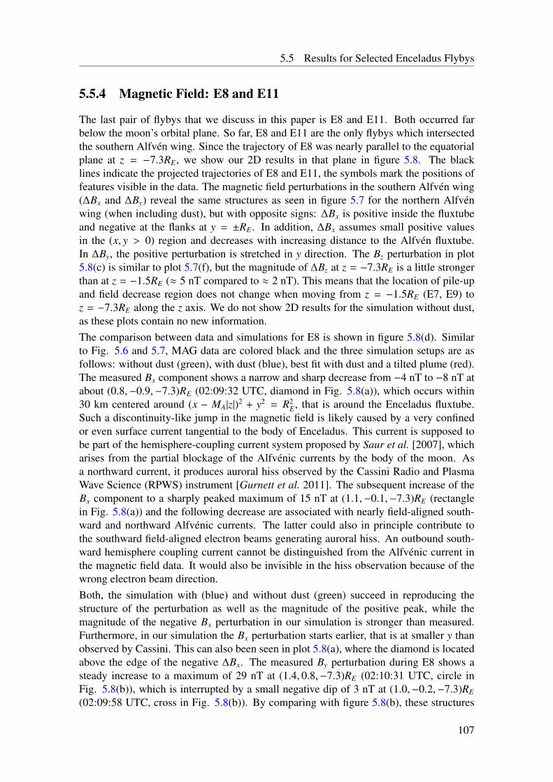
5.5 Results for Selected Enceladus Flybys
5.5.4 Magnetic Field: E8 and E11
The last pair of flybys that we discuss in this paper is E8 and E11. Both occurred farbelow the moon’s orbital plane. So far, E8 and E11 are the only flybys which intersectedthe southern Alfvén wing. Since the trajectory of E8 was nearly parallel to the equatorialplane at z = −7.3RE, we show our 2D results in that plane in figure 5.8. The blacklines indicate the projected trajectories of E8 and E11, the symbols mark the positions offeatures visible in the data. The magnetic field perturbations in the southern Alfvén wing(∆Bx and ∆By) reveal the same structures as seen in figure 5.7 for the northern Alfvénwing (when including dust), but with opposite signs: ∆Bx is positive inside the fluxtubeand negative at the flanks at y = ±RE. In addition, ∆Bx assumes small positive valuesin the (x, y > 0) region and decreases with increasing distance to the Alfvén fluxtube.In ∆By, the positive perturbation is stretched in y direction. The Bz perturbation in plot5.8(c) is similar to plot 5.7(f), but the magnitude of ∆Bz at z = −7.3RE is a little strongerthan at z = −1.5RE (≈ 5 nT compared to ≈ 2 nT). This means that the location of pile-upand field decrease region does not change when moving from z = −1.5RE (E7, E9) toz = −7.3RE along the z axis. We do not show 2D results for the simulation without dust,as these plots contain no new information.The comparison between data and simulations for E8 is shown in figure 5.8(d). Similarto Fig. 5.6 and 5.7, MAG data are colored black and the three simulation setups are asfollows: without dust (green), with dust (blue), best fit with dust and a tilted plume (red).The measured Bx component shows a narrow and sharp decrease from −4 nT to −8 nT atabout (0.8,−0.9,−7.3)RE (02:09:32 UTC, diamond in Fig. 5.8(a)), which occurs within30 km centered around (x − MA|z|)2 + y2 = R2
E, that is around the Enceladus fluxtube.Such a discontinuity-like jump in the magnetic field is likely caused by a very confinedor even surface current tangential to the body of Enceladus. This current is supposed tobe part of the hemisphere-coupling current system proposed by Saur et al. [2007], whicharises from the partial blockage of the Alfvénic currents by the body of the moon. Asa northward current, it produces auroral hiss observed by the Cassini Radio and PlasmaWave Science (RPWS) instrument [Gurnett et al. 2011]. The subsequent increase of theBx component to a sharply peaked maximum of 15 nT at (1.1,−0.1,−7.3)RE (rectanglein Fig. 5.8(a)) and the following decrease are associated with nearly field-aligned south-ward and northward Alfvénic currents. The latter could also in principle contribute tothe southward field-aligned electron beams generating auroral hiss. An outbound south-ward hemisphere coupling current cannot be distinguished from the Alfvénic current inthe magnetic field data. It would also be invisible in the hiss observation because of thewrong electron beam direction.Both, the simulation with (blue) and without dust (green) succeed in reproducing thestructure of the perturbation as well as the magnitude of the positive peak, while themagnitude of the negative Bx perturbation in our simulation is stronger than measured.Furthermore, in our simulation the Bx perturbation starts earlier, that is at smaller y thanobserved by Cassini. This can also been seen in plot 5.8(a), where the diamond is locatedabove the edge of the negative ∆Bx. The measured By perturbation during E8 shows asteady increase to a maximum of 29 nT at (1.4, 0.8,−7.3)RE (02:10:31 UTC, circle inFig. 5.8(b)), which is interrupted by a small negative dip of 3 nT at (1.0,−0.2,−7.3)RE
(02:09:58 UTC, cross in Fig. 5.8(b)). By comparing with figure 5.8(b), these structures
107
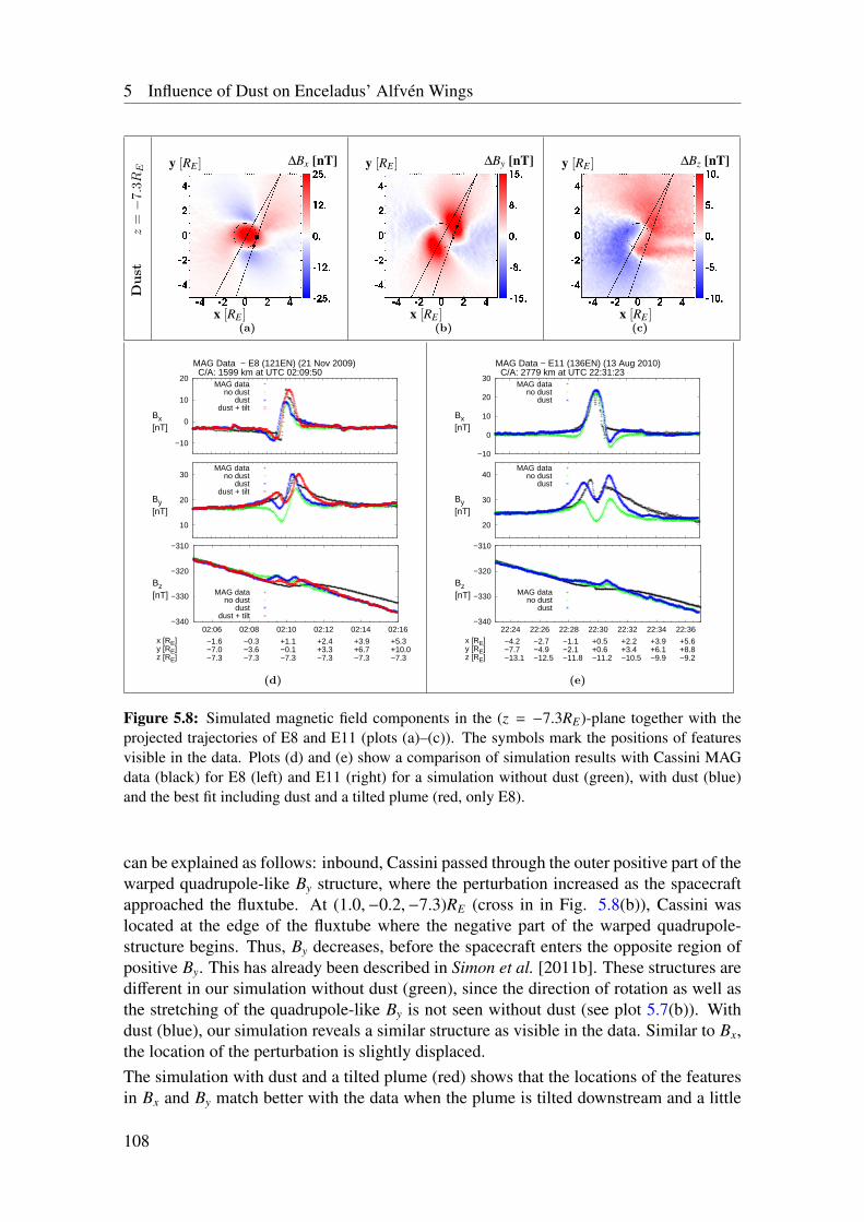
5 Influence of Dust on Enceladus’ Alfvén Wings
Dust
z=−
7.3R
E
x [RE ]
y [RE ] ∆Bx [nT]
1
(a)x [RE ]
y [RE ] ∆By [nT]
1
(b)x [RE ]
y [RE ] ∆Bz [nT]
1
(c)
−10
0
10
20
02:05 02:06 02:07 02:08 02:09 02:10 02:11 02:12 02:13 02:14 02:15 02:16
MAG Data − E8 (121EN) (21 Nov 2009) C/A: 1599 km at UTC 02:09:50
Bx [nT]
MAG datano dust
dustdust + tilt
10
20
30
02:05 02:06 02:07 02:08 02:09 02:10 02:11 02:12 02:13 02:14 02:15 02:16
By [nT]
MAG datano dust
dustdust + tilt
−340
−330
−320
−310
02:06 02:08 02:10 02:12 02:14 02:16x [RE]y [RE]z [RE]
−1.6−7.0−7.3
−0.3−3.6−7.3
+1.1−0.1−7.3
+2.4+3.3−7.3
+3.9+6.7−7.3
+5.3+10.0−7.3
Bz [nT] MAG data
no dustdust
dust + tilt
(d)
−10
0
10
20
30
22:24 22:26 22:28 22:30 22:32 22:34 22:36
MAG Data − E11 (136EN) (13 Aug 2010) C/A: 2779 km at UTC 22:31:23
Bx [nT]
MAG datano dust
dust
20
30
40
22:24 22:26 22:28 22:30 22:32 22:34 22:36
By [nT]
MAG datano dust
dust
−340
−330
−320
−310
22:24 22:26 22:28 22:30 22:32 22:34 22:36x [RE]y [RE]z [RE]
−4.2−7.7−13.1
−2.7−4.9−12.5
−1.1−2.1−11.8
+0.5+0.6−11.2
+2.2+3.4−10.5
+3.9+6.1−9.9
+5.6+8.8−9.2
Bz [nT] MAG data
no dustdust
(e)
Figure 5.8: Simulated magnetic field components in the (z = −7.3RE)-plane together with theprojected trajectories of E8 and E11 (plots (a)–(c)). The symbols mark the positions of featuresvisible in the data. Plots (d) and (e) show a comparison of simulation results with Cassini MAGdata (black) for E8 (left) and E11 (right) for a simulation without dust (green), with dust (blue)and the best fit including dust and a tilted plume (red, only E8).
can be explained as follows: inbound, Cassini passed through the outer positive part of thewarped quadrupole-like By structure, where the perturbation increased as the spacecraftapproached the fluxtube. At (1.0,−0.2,−7.3)RE (cross in in Fig. 5.8(b)), Cassini waslocated at the edge of the fluxtube where the negative part of the warped quadrupole-structure begins. Thus, By decreases, before the spacecraft enters the opposite region ofpositive By. This has already been described in Simon et al. [2011b]. These structures aredifferent in our simulation without dust (green), since the direction of rotation as well asthe stretching of the quadrupole-like By is not seen without dust (see plot 5.7(b)). Withdust (blue), our simulation reveals a similar structure as visible in the data. Similar to Bx,the location of the perturbation is slightly displaced.The simulation with dust and a tilted plume (red) shows that the locations of the featuresin Bx and By match better with the data when the plume is tilted downstream and a little
108
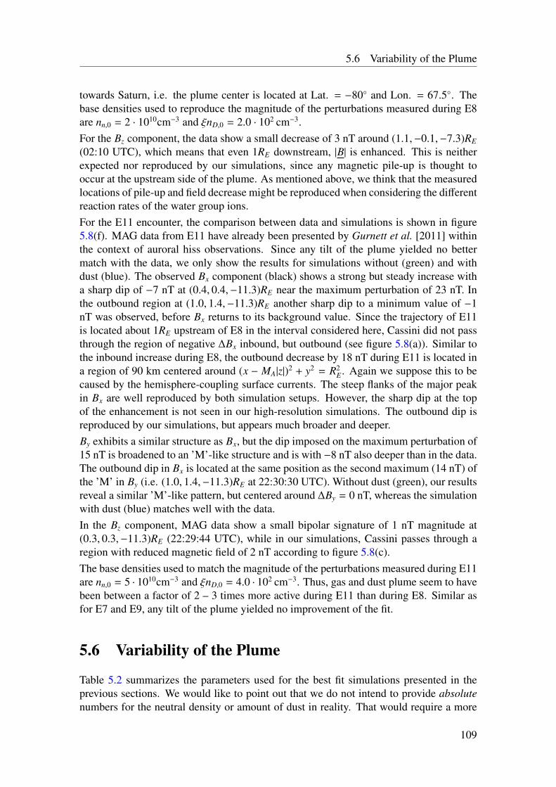
5.6 Variability of the Plume
towards Saturn, i.e. the plume center is located at Lat. = −80 and Lon. = 67.5. Thebase densities used to reproduce the magnitude of the perturbations measured during E8are nn,0 = 2 · 1010cm−3 and ξnD,0 = 2.0 · 102 cm−3.For the Bz component, the data show a small decrease of 3 nT around (1.1,−0.1,−7.3)RE
(02:10 UTC), which means that even 1RE downstream, |B| is enhanced. This is neitherexpected nor reproduced by our simulations, since any magnetic pile-up is thought tooccur at the upstream side of the plume. As mentioned above, we think that the measuredlocations of pile-up and field decrease might be reproduced when considering the differentreaction rates of the water group ions.For the E11 encounter, the comparison between data and simulations is shown in figure5.8(f). MAG data from E11 have already been presented by Gurnett et al. [2011] withinthe context of auroral hiss observations. Since any tilt of the plume yielded no bettermatch with the data, we only show the results for simulations without (green) and withdust (blue). The observed Bx component (black) shows a strong but steady increase witha sharp dip of −7 nT at (0.4, 0.4,−11.3)RE near the maximum perturbation of 23 nT. Inthe outbound region at (1.0, 1.4,−11.3)RE another sharp dip to a minimum value of −1nT was observed, before Bx returns to its background value. Since the trajectory of E11is located about 1RE upstream of E8 in the interval considered here, Cassini did not passthrough the region of negative ∆Bx inbound, but outbound (see figure 5.8(a)). Similar tothe inbound increase during E8, the outbound decrease by 18 nT during E11 is located ina region of 90 km centered around (x − MA|z|)2 + y2 = R2
E. Again we suppose this to becaused by the hemisphere-coupling surface currents. The steep flanks of the major peakin Bx are well reproduced by both simulation setups. However, the sharp dip at the topof the enhancement is not seen in our high-resolution simulations. The outbound dip isreproduced by our simulations, but appears much broader and deeper.By exhibits a similar structure as Bx, but the dip imposed on the maximum perturbation of15 nT is broadened to an ’M’-like structure and is with −8 nT also deeper than in the data.The outbound dip in Bx is located at the same position as the second maximum (14 nT) ofthe ’M’ in By (i.e. (1.0, 1.4,−11.3)RE at 22:30:30 UTC). Without dust (green), our resultsreveal a similar ’M’-like pattern, but centered around ∆By = 0 nT, whereas the simulationwith dust (blue) matches well with the data.In the Bz component, MAG data show a small bipolar signature of 1 nT magnitude at(0.3, 0.3,−11.3)RE (22:29:44 UTC), while in our simulations, Cassini passes through aregion with reduced magnetic field of 2 nT according to figure 5.8(c).The base densities used to match the magnitude of the perturbations measured during E11are nn,0 = 5 · 1010cm−3 and ξnD,0 = 4.0 · 102 cm−3. Thus, gas and dust plume seem to havebeen between a factor of 2 – 3 times more active during E11 than during E8. Similar asfor E7 and E9, any tilt of the plume yielded no improvement of the fit.
5.6 Variability of the Plume
Table 5.2 summarizes the parameters used for the best fit simulations presented in theprevious sections. We would like to point out that we do not intend to provide absolutenumbers for the neutral density or amount of dust in reality. That would require a more
109
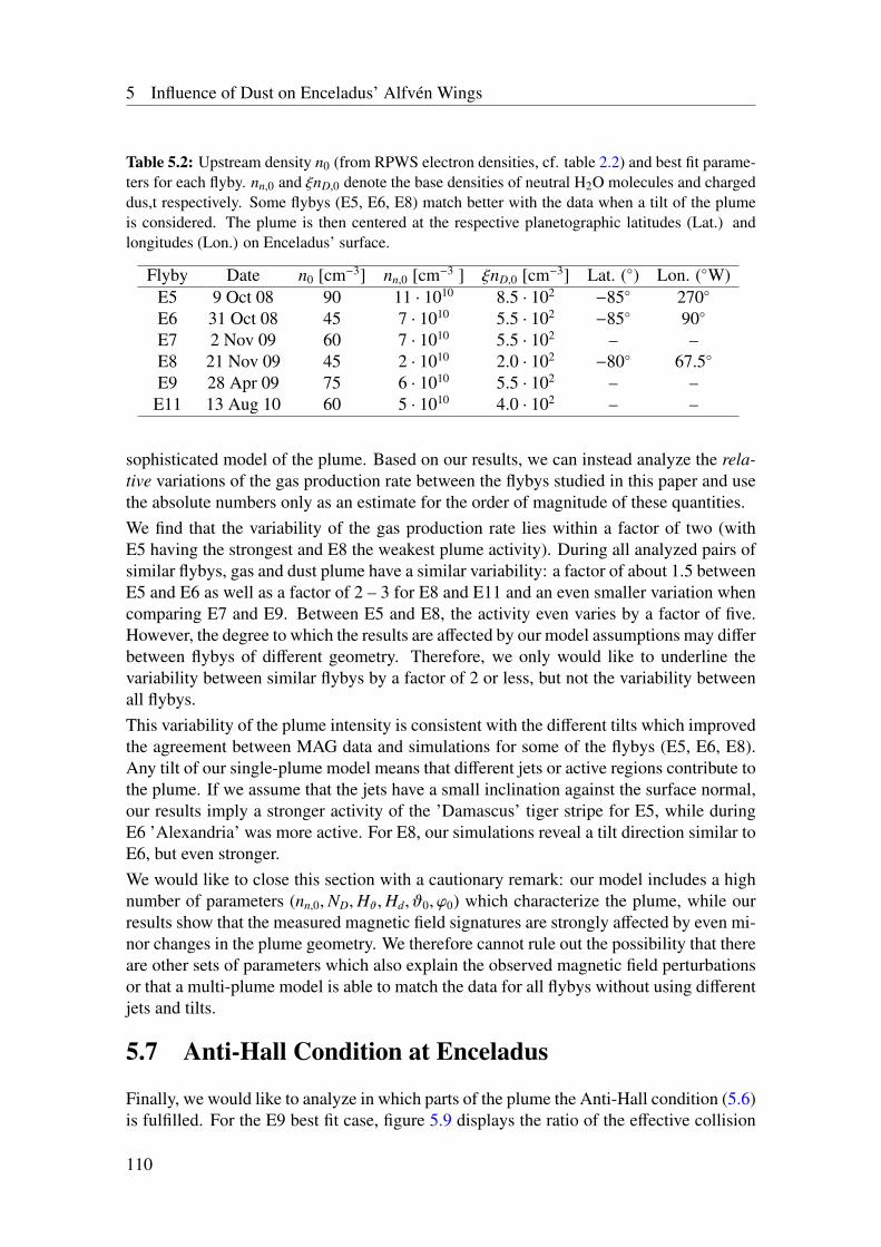
5 Influence of Dust on Enceladus’ Alfvén Wings
Table 5.2: Upstream density n0 (from RPWS electron densities, cf. table 2.2) and best fit parame-ters for each flyby. nn,0 and ξnD,0 denote the base densities of neutral H2O molecules and chargeddus,t respectively. Some flybys (E5, E6, E8) match better with the data when a tilt of the plumeis considered. The plume is then centered at the respective planetographic latitudes (Lat.) andlongitudes (Lon.) on Enceladus’ surface.
Flyby Date n0 [cm−3] nn,0 [cm−3 ] ξnD,0 [cm−3] Lat. () Lon. (W)E5 9 Oct 08 90 11 · 1010 8.5 · 102 −85 270
E6 31 Oct 08 45 7 · 1010 5.5 · 102 −85 90
E7 2 Nov 09 60 7 · 1010 5.5 · 102 – –E8 21 Nov 09 45 2 · 1010 2.0 · 102 −80 67.5
E9 28 Apr 09 75 6 · 1010 5.5 · 102 – –E11 13 Aug 10 60 5 · 1010 4.0 · 102 – –
sophisticated model of the plume. Based on our results, we can instead analyze the rela-tive variations of the gas production rate between the flybys studied in this paper and usethe absolute numbers only as an estimate for the order of magnitude of these quantities.We find that the variability of the gas production rate lies within a factor of two (withE5 having the strongest and E8 the weakest plume activity). During all analyzed pairs ofsimilar flybys, gas and dust plume have a similar variability: a factor of about 1.5 betweenE5 and E6 as well as a factor of 2 – 3 for E8 and E11 and an even smaller variation whencomparing E7 and E9. Between E5 and E8, the activity even varies by a factor of five.However, the degree to which the results are affected by our model assumptions may differbetween flybys of different geometry. Therefore, we only would like to underline thevariability between similar flybys by a factor of 2 or less, but not the variability betweenall flybys.This variability of the plume intensity is consistent with the different tilts which improvedthe agreement between MAG data and simulations for some of the flybys (E5, E6, E8).Any tilt of our single-plume model means that different jets or active regions contribute tothe plume. If we assume that the jets have a small inclination against the surface normal,our results imply a stronger activity of the ’Damascus’ tiger stripe for E5, while duringE6 ’Alexandria’ was more active. For E8, our simulations reveal a tilt direction similar toE6, but even stronger.We would like to close this section with a cautionary remark: our model includes a highnumber of parameters (nn,0,ND,Hϑ,Hd, ϑ0, ϕ0) which characterize the plume, while ourresults show that the measured magnetic field signatures are strongly affected by even mi-nor changes in the plume geometry. We therefore cannot rule out the possibility that thereare other sets of parameters which also explain the observed magnetic field perturbationsor that a multi-plume model is able to match the data for all flybys without using differentjets and tilts.
5.7 Anti-Hall Condition at Enceladus
Finally, we would like to analyze in which parts of the plume the Anti-Hall condition (5.6)is fulfilled. For the E9 best fit case, figure 5.9 displays the ratio of the effective collision
110
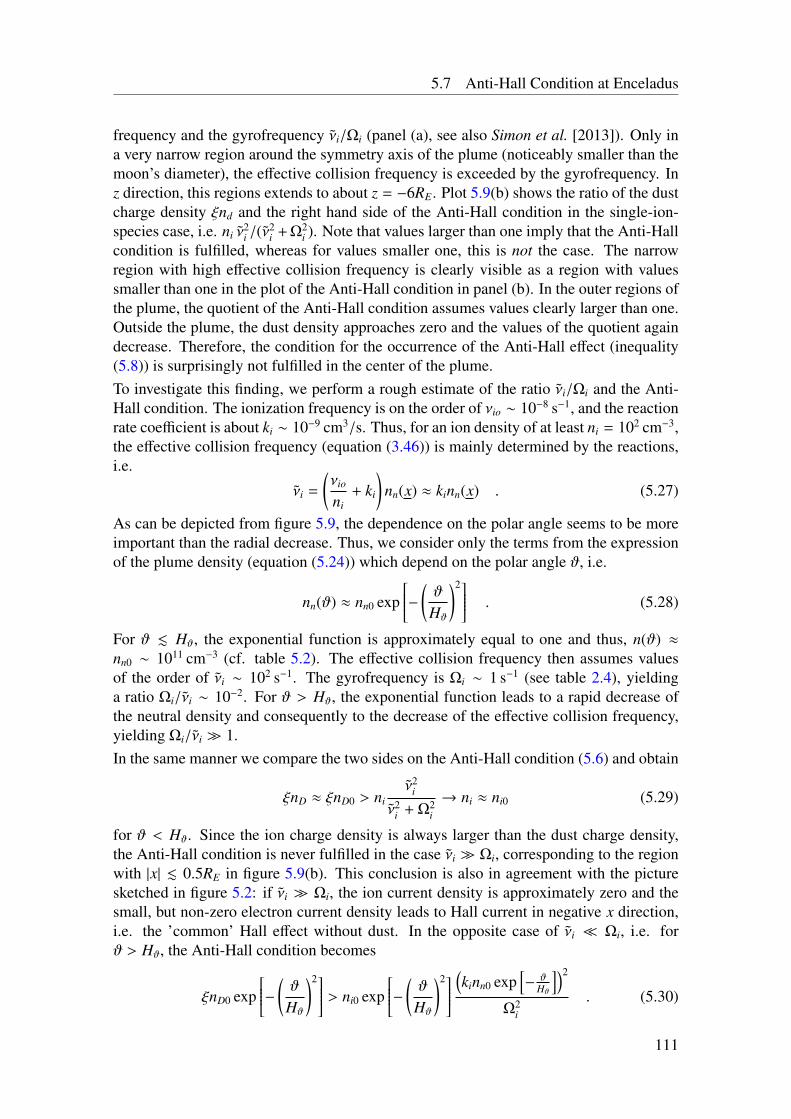
5.7 Anti-Hall Condition at Enceladus
frequency and the gyrofrequency νi/Ωi (panel (a), see also Simon et al. [2013]). Only ina very narrow region around the symmetry axis of the plume (noticeably smaller than themoon’s diameter), the effective collision frequency is exceeded by the gyrofrequency. Inz direction, this regions extends to about z = −6RE. Plot 5.9(b) shows the ratio of the dustcharge density ξnd and the right hand side of the Anti-Hall condition in the single-ion-species case, i.e. ni ν
2i /(ν
2i + Ω2
i ). Note that values larger than one imply that the Anti-Hallcondition is fulfilled, whereas for values smaller one, this is not the case. The narrowregion with high effective collision frequency is clearly visible as a region with valuessmaller than one in the plot of the Anti-Hall condition in panel (b). In the outer regions ofthe plume, the quotient of the Anti-Hall condition assumes values clearly larger than one.Outside the plume, the dust density approaches zero and the values of the quotient againdecrease. Therefore, the condition for the occurrence of the Anti-Hall effect (inequality(5.8)) is surprisingly not fulfilled in the center of the plume.To investigate this finding, we perform a rough estimate of the ratio νi/Ωi and the Anti-Hall condition. The ionization frequency is on the order of νio ∼ 10−8 s−1, and the reactionrate coefficient is about ki ∼ 10−9 cm3/s. Thus, for an ion density of at least ni = 102 cm−3,the effective collision frequency (equation (3.46)) is mainly determined by the reactions,i.e.
νi =
(νio
ni+ ki
)nn(x) ≈ kinn(x) . (5.27)
As can be depicted from figure 5.9, the dependence on the polar angle seems to be moreimportant than the radial decrease. Thus, we consider only the terms from the expressionof the plume density (equation (5.24)) which depend on the polar angle ϑ, i.e.
nn(ϑ) ≈ nn0 exp− (
ϑ
Hϑ
)2 . (5.28)
For ϑ . Hϑ, the exponential function is approximately equal to one and thus, n(ϑ) ≈nn0 ∼ 1011 cm−3 (cf. table 5.2). The effective collision frequency then assumes valuesof the order of νi ∼ 102 s−1. The gyrofrequency is Ωi ∼ 1 s−1 (see table 2.4), yieldinga ratio Ωi/νi ∼ 10−2. For ϑ > Hϑ, the exponential function leads to a rapid decrease ofthe neutral density and consequently to the decrease of the effective collision frequency,yielding Ωi/νi 1.In the same manner we compare the two sides on the Anti-Hall condition (5.6) and obtain
ξnD ≈ ξnD0 > niν2
i
ν2i + Ω2
i
→ ni ≈ ni0 (5.29)
for ϑ < Hϑ. Since the ion charge density is always larger than the dust charge density,the Anti-Hall condition is never fulfilled in the case νi Ωi, corresponding to the regionwith |x| . 0.5RE in figure 5.9(b). This conclusion is also in agreement with the picturesketched in figure 5.2: if νi Ωi, the ion current density is approximately zero and thesmall, but non-zero electron current density leads to Hall current in negative x direction,i.e. the ’common’ Hall effect without dust. In the opposite case of νi Ωi, i.e. forϑ > Hϑ, the Anti-Hall condition becomes
ξnD0 exp− (
ϑ
Hϑ
)2 > ni0 exp− (
ϑ
Hϑ
)2(kinn0 exp
[− ϑ
Hϑ
])2
Ω2i
. (5.30)
111
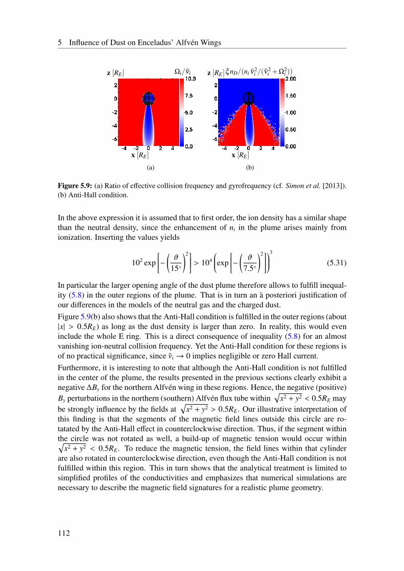
5 Influence of Dust on Enceladus’ Alfvén Wings
x [RE ]
z [RE ] Ωi/νi
1
(a)
x [RE ]
z [RE ]ξ nD/(ni ν2i /(ν2
i +Ω2i ))
1
(b)
Figure 5.9: (a) Ratio of effective collision frequency and gyrofrequency (cf. Simon et al. [2013]).(b) Anti-Hall condition.
In the above expression it is assumed that to first order, the ion density has a similar shapethan the neutral density, since the enhancement of ni in the plume arises mainly fromionization. Inserting the values yields
102 exp− (
ϑ
15
)2 > 104
exp− (
ϑ
7.5
)23
(5.31)
In particular the larger opening angle of the dust plume therefore allows to fulfill inequal-ity (5.8) in the outer regions of the plume. That is in turn an à posteriori justification ofour differences in the models of the neutral gas and the charged dust.Figure 5.9(b) also shows that the Anti-Hall condition is fulfilled in the outer regions (about|x| > 0.5RE) as long as the dust density is larger than zero. In reality, this would eveninclude the whole E ring. This is a direct consequence of inequality (5.8) for an almostvanishing ion-neutral collision frequency. Yet the Anti-Hall condition for these regions isof no practical significance, since νi → 0 implies negligible or zero Hall current.Furthermore, it is interesting to note that although the Anti-Hall condition is not fulfilledin the center of the plume, the results presented in the previous sections clearly exhibit anegative ∆By for the northern Alfvén wing in these regions. Hence, the negative (positive)By perturbations in the northern (southern) Alfvén flux tube within
√x2 + y2 < 0.5RE may
be strongly influence by the fields at√
x2 + y2 > 0.5RE. Our illustrative interpretation ofthis finding is that the segments of the magnetic field lines outside this circle are ro-tatated by the Anti-Hall effect in counterclockwise direction. Thus, if the segment withinthe circle was not rotated as well, a build-up of magnetic tension would occur within√
x2 + y2 < 0.5RE. To reduce the magnetic tension, the field lines within that cylinderare also rotated in counterclockwise direction, even though the Anti-Hall condition is notfulfilled within this region. This in turn shows that the analytical treatment is limited tosimplified profiles of the conductivities and emphasizes that numerical simulations arenecessary to describe the magnetic field signatures for a realistic plume geometry.
112
6 Ion Densities and MagneticSignatures of Dust Pick-up atEnceladus
Wide parts of the following chapter have been submitted for publication before submis-sion of the thesis. The publication is referred to as:Kriegel, H., S. Simon, P. Meier, U. Motschmann, J. Saur, A. Wennmacher, D. F. Strobel,and M. K. Dougherty, Ion Densities and Magnetic Signatures of Dust Pick-Up at Ence-ladus, submitted to Journal of Geophysical Research (Space Physics)
The main result presented in the previous chapter was the successful reproduction ofthe field perturbations associated with the Anti-Hall effect, although simplified analyticalexpressions adopted from the work of Saur et al. [2008] for the neutral and dust plumeswere applied. The free parameters in these expressions were adjusted to MAG data fromselected Enceladus flybys. A major drawback of this method is that the modification of theplume due to the pick-up motion of charged dust grains is not included. Furthermore, onlyone instrument of Cassini – MAG – has been used to analyze the plasma interaction. Herewe present an improved version of the model which includes Monte-Carlo simulations ofthe neutral gas and dust plumes. The resulting neutral plume is consistent with INMSdata and the parameters of the dust plume are chosen in agreement with CDA and CAPSobservations. In particular, the model now contains the full dust-plasma coupling in bothdirections, i. e. the dust is affected by the electromagnetic fields and plasma moments andvice versa. Thus we are now able to address several open questions on Enceladus’ plasmainteraction:
• Ion and dust charge densities in the plume: We combine our plume model withrealistic ionization frequencies to impose constraints on the ion and dust chargedensities in the plume and compare these expectations against the values directlyor indirectly derived from data collected by Cassini’s CAPS, RPWS and INMSinstruments.
• Magnetic signatures of dust pick-up: In the previous chapter, we have shown thatthe presence of negatively charged dust is responsible for the Anti-Hall effect, i. e.the reversal of the (anti-)Saturnward magnetic field component. Here we are goingto discuss how the shape of the dust plume is responsible for the observed magneticfield signatures and deduce properties of the dust plume.
113
6 Ion Densities and Magnetic Signatures of Dust Pick-up at Enceladus
• The missing magnetic field decrease: During E0 – E19, the Cassini magnetometerhas observed only the magnetic pile-up region at the ramside of the plume. Despitea good flyby coverage at the moon’s wakeside, the corresponding magnetic fielddecrease has not yet been detected. We demonstrate that the modification of thecurrent systems by the charged dust grains shifted the magnetic field decrease outof Cassini’s path during all available Enceladus encounters.
Within this chapter we are going to focus on a few selected flybys which are particularlysuitable to deal with the aforementioned issues. These flybys are E3, E5, E7, and themore recent encounters E14, E15, E17, E18 and E19. All flybys not addressed in this orthe previous chapter are discussed in appendix B. The reason for our selection of theseparticular flybys is that for E3 and E5, INMS, CAPS and RPWS data are available, whatallows us to constrain the ion densities in the plume [Morooka et al. 2011, Teolis et al.2010, Hill et al. 2012]. Magnetic field data and simulations for E7 and E9 have alreadybeen presented in section 5.5.3. Therefore, E7 provides a reference to illustrate the ef-fect of the improvements included in the model. The magnetic field signatures observedduring the encounters E14, E17 and E18 show only minor quantitative differences. Forthis reason, we decided to discuss E14 and E17 in detail, while magnetic field data fromE18 is used only for a brief analysis of plume variability. The comparison of these flybyswith E19 is especially important for an understanding of the magnetic field decrease. Thedistant E15 encounter provides the unique opportunity to analyze the pick-up tail of theplume at large distances to Enceladus. In contrast, the north polar E12 and E13 flybys didnot pass through the plume and are therefore discussed only in appendix B. Furthermore,since the trajectory of E16 is very similar to E1 and E10, the magnetic field signaturesobtained during this flyby do not contain any new substantial information. Therefore, dataand simulations for E16 are shown in appendix B only for completeness.
6.1 Simulation Model
In this chapter a new simulation principle is introduced: we combine the plasma simula-tion with Monte-Carlo simulations of both, the H2O and the dust plume. In contrast toour previous study, we do not only consider the influence of electron absorption by dustgrains on the electromagnetic fields and plasma flow patterns, but the feedback of thelocal plasma environment on the motion and charging of the dust. The major challengeof such a model arises from the differences of the involved time scales: on the one hand,the time scale for stationarity of the plasma simulation is roughly defined by the time τp
that is required by the decelerated plasma flow to travel through the plume in corotationdirection, i. e. τp = 2RE/1 km s−1 ≈ 500 s. On the other hand, the Monte-Carlo simu-lations achieve stationarity on a time scale τMC corresponding to the time that the slowneutral molecules or dust grains need to cross the plume in north-south direction, i. e.τMC = 20RE/0.5 km s−1 ∼ 10000 s. With the available computational resources it is notpossible to combine both time scales in a single simulation. Instead, we have developedan iterative scheme of three different types of simulations which provide the input for eachother:
(1) A ”downgraded” version of our plasma simulation code is used for a Monte-Carlo
114
6.1 Simulation Model
Particle-in-Cell simulation which produces a 3D density and velocity profile of theneutral plume (see section 6.2).
(2) A plasma simulation with A.I.K.E.F. is carried out. Here, the 3D profile of the gasplume obtained by simulation (1) is used as stationary input. In this first step, thedust plume is provided by the model used for the previous simulations (see section5.4.3).
(3) Subsequently, a Monte-Carlo simulation is carried out for the dust plume (seesection 6.3). These simulations, however, require the electromagnetic fields andplasma densities from the hybrid simulations (2) as input to compute the grain dy-namics by the Lorentz force and the grain charging according to the plasma densi-ties.
(4) Next, we perform an improved plasma simulation with the gas and dust plumesfrom steps (1) and (3).
(5) Then an improved simulation of the dust plume with the electromagnetic fields andplasma densities from (4) is made.
(6) A final hybrid simulation with the gas and dust plumes from steps (1) and (5) iscarried out.
We find that after steps (5) and (6), the iteration scheme has reached a consistent state, i.e. a third simulation of the dust plume using the results from the hybrid simulation (6)does not lead to noticeable changes of the dust plume.Apart from the iterative simulation principle, the description of the ion-neutral chemistrywithin the plasma simulations has been improved and will be discussed in sections 6.1.2and 6.1.3. The physical and numerical input parameters of the simulations are summa-rized in the following section.
6.1.1 Simulation Parameters
Although we have used a dipolar background magnetic field in the previous chapter, wedecided to use the more simple case of a constant background field B0 = −B0ez for thesimulations presented in this chapter since both approaches do not make any difference forthe results. The magnitude of the background field as well as other physical parameters ofthe upstream plasma are listed in table 6.1. Again, we adjust the upstream density for thesimulation of each flyby according to the upstream electron densities derived from RPWSmeasurements of the upper hybrid frequency, which are listed in table 2.2. In contrastto our previous simulations, we now consider the finding that the speed of the upstreamplasma relative to Enceladus is about 80% of the rigid corotation velocity of 26.4 km/s,i. e. u0 = 21.1 km/s [Wilson et al. 2009]. From these numbers and for water group ionswith an average mass of mW+ = 17.5 amu, we derive an Alfvén Mach number betweenMA = 0.08 and MA = 0.13. Furthermore, we now take into account the temperatureanisotropy, i.e. the ratio of the water group ion temperatures perpendicular and parallel tothe ambient magnetic field is about Ti⊥/Ti‖ = 5, see equation (2.4) and Sittler et al. [2006].
115
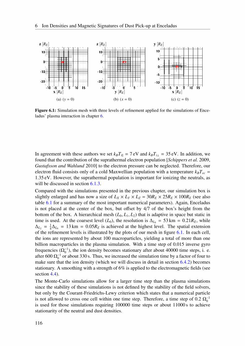
6 Ion Densities and Magnetic Signatures of Dust Pick-up at Enceladus
x [RE ]
z [RE ]
1
(a) (y = 0)
y [RE ]
z [RE ]
1
(b) (x = 0)
x [RE ]
y [RE ]
1
(c) (z = 0)
Figure 6.1: Simulation mesh with three levels of refinement applied for the simulations of Ence-ladus’ plasma interaction in chapter 6.
In agreement with these authors we set kBTi‖ = 7 eV and kBTi⊥ = 35 eV. In addition, wefound that the contribution of the suprathermal electron population [Schippers et al. 2009,Gustafsson and Wahlund 2010] to the electron pressure can be neglected. Therefore, ourelectron fluid consists only of a cold Maxwellian population with a temperature kBTec =
1.35 eV. However, the suprathermal population is important for ionizing the neutrals, aswill be discussed in section 6.1.3.Compared with the simulations presented in the previous chapter, our simulation box isslightly enlarged and has now a size of LX × LY × LZ = 30RE × 25RE × 100RE (see alsotable 6.1 for a summary of the most important numerical parameters). Again, Enceladusis not placed at the center of the box, but offset by 4/7 of the box’s height from thebottom of the box. A hierarchical mesh (L0, L1, L2) that is adaptive in space but static intime is used. At the coarsest level (L0), the resolution is ∆L0 = 53 km = 0.21RE, while∆L2 = 1
4∆L0 = 13 km = 0.05RE is achieved at the highest level. The spatial extensionof the refinement levels is illustrated by the plots of our mesh in figure 6.1. In each cell,the ions are represented by about 100 macroparticles, yielding a total of more than onebillion macroparticles in the plasma simulation. With a time step of 0.015 inverse gyrofrequencies (Ω−1
0 ), the ion density becomes stationary after about 40000 time steps, i. e.after 600 Ω−1
0 or about 330 s. Thus, we increased the simulation time by a factor of four tomake sure that the ion density (which we will discuss in detail in section 6.4.2) becomesstationary. A smoothing with a strength of 6% is applied to the electromagnetic fields (seesection 4.4).The Monte-Carlo simulations allow for a larger time step than the plasma simulationssince the stability of these simulations is not defined by the stability of the field solvers,but only by the Courant-Friedrichs-Lewy criterion which states that a numerical particleis not allowed to cross one cell within one time step. Therefore, a time step of 0.2 Ω−1
0is used for those simulations requiring 100000 time steps or about 11000 s to achievestationarity of the neutral and dust densities.
116
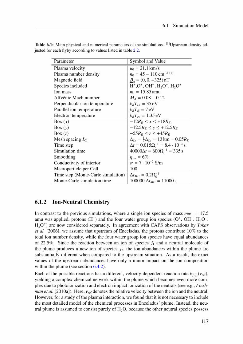
6.1 Simulation Model
Table 6.1: Main physical and numerical parameters of the simulations. [1]Upstream density ad-justed for each flyby according to values listed in table 2.2.
Parameter Symbol and ValuePlasma velocity u0 = 21.1 km/sPlasma number density n0 = 45 − 110 cm−3 [1]
Magnetic field B0 = (0, 0,−325) nTSpecies included H+,O+, OH+, H2O+, H3O+
Ion mass mi = 15.85 amuAlfvénic Mach number MA = 0.08 − 0.12Perpendicular ion temperature kBTi⊥ = 35 eVParallel ion temperature kBTi‖ = 7 eVElectron temperature kBTec = 1.35 eVBox (x) −12RE ≤ x ≤ +18RE
Box (y) −12.5RE ≤ y ≤ +12.5RE
Box (z) −55RE ≤ z ≤ +45RE
Mesh spacing L2 ∆L2 = 14∆L0 = 13 km = 0.05RE
Time step ∆t = 0.015Ω−1i = 8.4 · 10−3 s
Simulation time 40000∆t = 600Ω−1i = 335 s
Smoothing ηsm = 6%Conductivity of interior σ = 7 · 10−7 S/mMacroparticle per Cell 100Time step (Monte-Carlo simulation) ∆tMC = 0.2Ω−1
0Monte-Carlo simulation time 100000 ∆tMC = 11000 s
6.1.2 Ion-Neutral Chemistry
In contrast to the previous simulations, where a single ion species of mass mW+ = 17.5amu was applied, protons (H+) and the four water group ion species (O+, OH+, H2O+,H3O+) are now considered separately. In agreement with CAPS observations by Tokaret al. [2006], we assume that upstream of Enceladus, the protons contribute 10% to thetotal ion number density, while the four water group ion species have equal abundancesof 22.5%. Since the reaction between an ion of species j1 and a neutral molecule ofthe plume produces a new ion of species j2, the ion abundances within the plume aresubstantially different when compared to the upstream situation. As a result, the exactvalues of the upstream abundances have only a minor impact on the ion compositionwithin the plume (see section 6.4.2).Each of the possible reactions has a different, velocity-dependent reaction rate k j1 j2(vrel),yielding a complex chemical network within the plume which becomes even more com-plex due to photoionization and electron impact ionization of the neutrals (see e.g., Flesh-man et al. [2010a]). Here, vrel denotes the relative velocity between the ion and the neutral.However, for a study of the plasma interaction, we found that it is not necessary to includethe most detailed model of the chemical processes in Enceladus’ plume. Instead, the neu-tral plume is assumed to consist purely of H2O, because the other neutral species possess
117
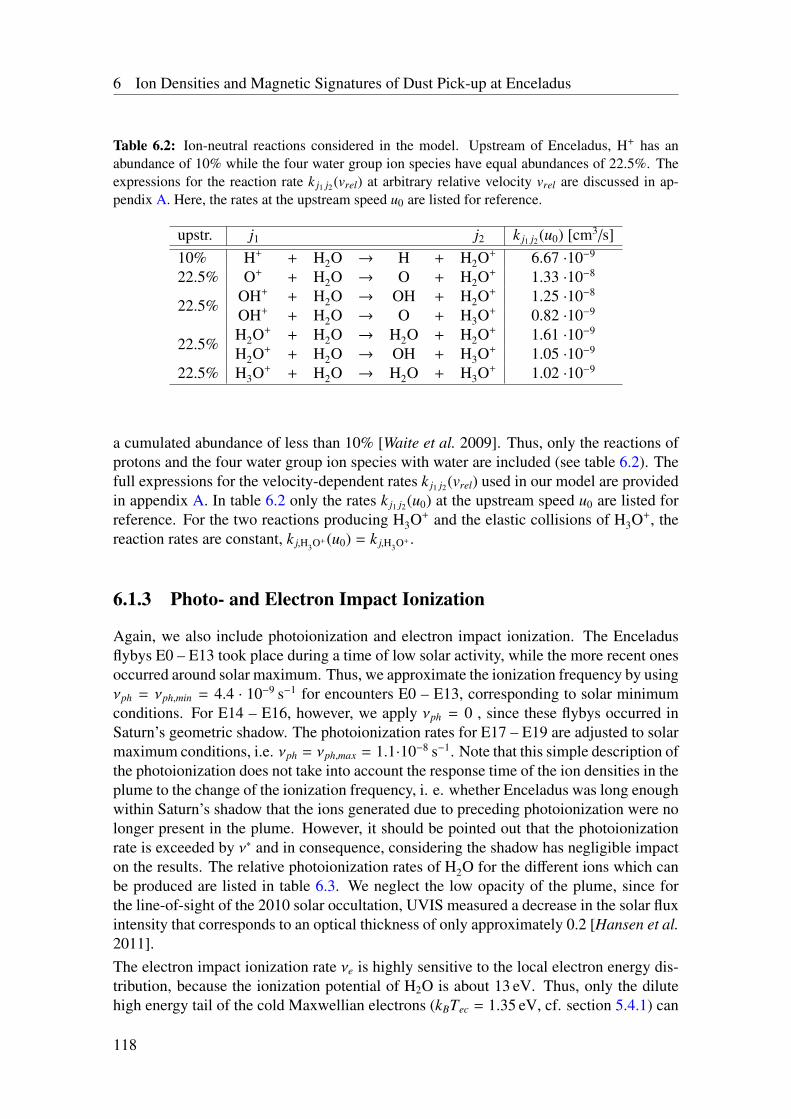
6 Ion Densities and Magnetic Signatures of Dust Pick-up at Enceladus
Table 6.2: Ion-neutral reactions considered in the model. Upstream of Enceladus, H+ has anabundance of 10% while the four water group ion species have equal abundances of 22.5%. Theexpressions for the reaction rate k j1 j2(vrel) at arbitrary relative velocity vrel are discussed in ap-pendix A. Here, the rates at the upstream speed u0 are listed for reference.
upstr. j1 j2 k j1 j2(u0) [cm3/s]10% H+ + H2O → H + H2O+ 6.67 ·10−9
22.5% O+ + H2O → O + H2O+ 1.33 ·10−8
22.5%OH+ + H2O → OH + H2O+ 1.25 ·10−8
OH+ + H2O → O + H3O+ 0.82 ·10−9
22.5%H2O+ + H2O → H2O + H2O+ 1.61 ·10−9
H2O+ + H2O → OH + H3O+ 1.05 ·10−9
22.5% H3O+ + H2O → H2O + H3O+ 1.02 ·10−9
a cumulated abundance of less than 10% [Waite et al. 2009]. Thus, only the reactions ofprotons and the four water group ion species with water are included (see table 6.2). Thefull expressions for the velocity-dependent rates k j1 j2(vrel) used in our model are providedin appendix A. In table 6.2 only the rates k j1 j2(u0) at the upstream speed u0 are listed forreference. For the two reactions producing H3O+ and the elastic collisions of H3O+, thereaction rates are constant, k j,H3O+(u0) = k j,H3O+ .
6.1.3 Photo- and Electron Impact Ionization
Again, we also include photoionization and electron impact ionization. The Enceladusflybys E0 – E13 took place during a time of low solar activity, while the more recent onesoccurred around solar maximum. Thus, we approximate the ionization frequency by usingνph = νph,min = 4.4 · 10−9 s−1 for encounters E0 – E13, corresponding to solar minimumconditions. For E14 – E16, however, we apply νph = 0 , since these flybys occurred inSaturn’s geometric shadow. The photoionization rates for E17 – E19 are adjusted to solarmaximum conditions, i.e. νph = νph,max = 1.1·10−8 s−1. Note that this simple description ofthe photoionization does not take into account the response time of the ion densities in theplume to the change of the ionization frequency, i. e. whether Enceladus was long enoughwithin Saturn’s shadow that the ions generated due to preceding photoionization were nolonger present in the plume. However, it should be pointed out that the photoionizationrate is exceeded by ν∗ and in consequence, considering the shadow has negligible impacton the results. The relative photoionization rates of H2O for the different ions which canbe produced are listed in table 6.3. We neglect the low opacity of the plume, since forthe line-of-sight of the 2010 solar occultation, UVIS measured a decrease in the solar fluxintensity that corresponds to an optical thickness of only approximately 0.2 [Hansen et al.2011].The electron impact ionization rate νe is highly sensitive to the local electron energy dis-tribution, because the ionization potential of H2O is about 13 eV. Thus, only the dilutehigh energy tail of the cold Maxwellian electrons (kBTec = 1.35 eV, cf. section 5.4.1) can
118
6.1 Simulation Model
contribute to the ionization while the major ionizing component is the suprathermal pop-ulation with electron energies of 10 − 70 eV. Recently, Ozak et al. [2012] applied a two-stream electron transport model to the suprathermal electrons within the plume in agree-ment with data obtained by the Electron Spectrometer (ELS) of CAPS. These authors con-cluded that the total ionization rate by electrons is in the range of νe,min = (1.2−2)·10−9 s−1
for solar minimum conditions. The interval of the νe,min values results from the opacity ofthe plume with respect to the ionizing electrons. As the opacity is again rather low, wesimply use an average value of νe,min = 1.5 · 10−9 s−1. Since the suprathermal electronsare mainly generated by photoionization of neutrals [Schippers et al. 2009], we increasethe rate by the same factor of 2.5 as the photoionization rate for solar maximum yieldingνe,max = 3.75 · 10−9 s−1. As these electrons are not necessarily produced at Enceladus, butsomewhere around its orbit, Saturn’s shadow is not considered for the electron ionization.The electron impact rates for the different ion species are obtained by using the same frac-tion of the total rate as for the photoionization (see table 6.3). This is also in agreementwith electron impact ionization cross sections from Itikawa and Mason [2005]. Note thatwe do not include a modification of the electron impact rate due to electron absorptionby dust. This would require a model of the electron energy distribution that considerscooling or heating of the electrons by the dust as well as the energy dependence of theelectron absorption.Since the model of Ozak et al. [2012] underestimates the electron fluxes at energies be-tween 100 eV and 1000 eV compared to CAPS measurements (see figures 11 and 12 inthat work), it shall be analyzed if this regime contributes significantly to the electron im-pact ionization. The ionization frequency can be calculated as (cf. eq. (4) of Burger et al.[2007])
νe = ne
∫σ(v) f (v)vdv , (6.1)
where σ(v) is the velocity-dependent ionization cross section and f (v) the velocity distri-bution of the electrons with < v >=
∫f (v)vdv. We are interested in a rough estimate of
the upper limit of νe, considering contributions by electrons with energies only between100 eV and 1000 eV. Furthermore, we assume that the electron flux Fe is isotropic and ofthe order of Fe = 102 cm−2s−1eV−1sr−1 within this energy interval in agreement with theCAPS observations presented by Ozak et al. [2012]. The flux can then be converted intoan electron density according to
ne
∫f (v)vdv = Fe4π∆E . (6.2)
For this energy interval, the electron impact cross section is nearly constant, σ(v) ∼10−16 cm−2 [Itikawa and Mason 2005]. Inserting equation (6.2) in (6.1) yields the ion-ization rate in the interval between 100 eV and 1000 eV,
νe = 4πFe∆Eσ(v) ∼ 1 · 10−10 s−1 . (6.3)
Thus, the electron impact ionization by electrons with energies larger than 100 eV yieldsan ionization frequency that is about one order of magnitude lower than the ionizationfrequency of the suprathermal electron population.In addition to the ion species included in the model, data obtained by INMS and CAPSsuggest the presence of heavier water cluster ions (H2O+-H2O or H3O+-H2O), with count
119
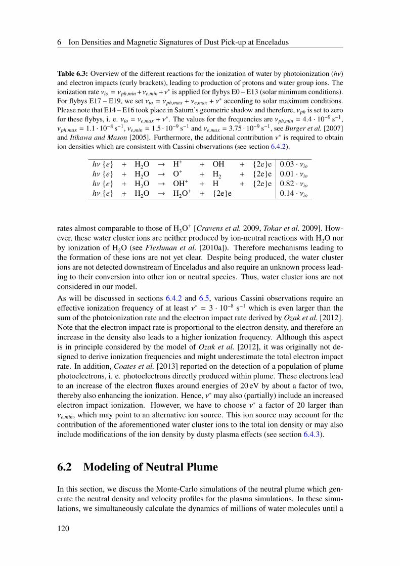
6 Ion Densities and Magnetic Signatures of Dust Pick-up at Enceladus
Table 6.3: Overview of the different reactions for the ionization of water by photoionization (hν)and electron impacts (curly brackets), leading to production of protons and water group ions. Theionization rate νio = νph,min +νe,min +ν∗ is applied for flybys E0 – E13 (solar minimum conditions).For flybys E17 – E19, we set νio = νph,max + νe,max + ν∗ according to solar maximum conditions.Please note that E14 – E16 took place in Saturn’s geometric shadow and therefore, νph is set to zerofor these flybys, i. e. νio = νe,max + ν∗. The values for the frequencies are νph,min = 4.4 · 10−9 s−1,νph,max = 1.1 · 10−8 s−1, νe,min = 1.5 · 10−9 s−1 and νe,max = 3.75 · 10−9 s−1, see Burger et al. [2007]and Itikawa and Mason [2005]. Furthermore, the additional contribution ν∗ is required to obtainion densities which are consistent with Cassini observations (see section 6.4.2).
hν e + H2O → H+ + OH + 2ee 0.03 · νio
hν e + H2O → O+ + H2 + 2ee 0.01 · νio
hν e + H2O → OH+ + H + 2ee 0.82 · νio
hν e + H2O → H2O+ + 2ee 0.14 · νio
rates almost comparable to those of H3O+ [Cravens et al. 2009, Tokar et al. 2009]. How-ever, these water cluster ions are neither produced by ion-neutral reactions with H2O norby ionization of H2O (see Fleshman et al. [2010a]). Therefore mechanisms leading tothe formation of these ions are not yet clear. Despite being produced, the water clusterions are not detected downstream of Enceladus and also require an unknown process lead-ing to their conversion into other ion or neutral species. Thus, water cluster ions are notconsidered in our model.As will be discussed in sections 6.4.2 and 6.5, various Cassini observations require aneffective ionization frequency of at least ν∗ = 3 · 10−8 s−1 which is even larger than thesum of the photoionization rate and the electron impact rate derived by Ozak et al. [2012].Note that the electron impact rate is proportional to the electron density, and therefore anincrease in the density also leads to a higher ionization frequency. Although this aspectis in principle considered by the model of Ozak et al. [2012], it was originally not de-signed to derive ionization frequencies and might underestimate the total electron impactrate. In addition, Coates et al. [2013] reported on the detection of a population of plumephotoelectrons, i. e. photoelectrons directly produced within plume. These electrons leadto an increase of the electron fluxes around energies of 20 eV by about a factor of two,thereby also enhancing the ionization. Hence, ν∗ may also (partially) include an increasedelectron impact ionization. However, we have to choose ν∗ a factor of 20 larger thanνe,min, which may point to an alternative ion source. This ion source may account for thecontribution of the aforementioned water cluster ions to the total ion density or may alsoinclude modifications of the ion density by dusty plasma effects (see section 6.4.3).
6.2 Modeling of Neutral Plume
In this section, we discuss the Monte-Carlo simulations of the neutral plume which gen-erate the neutral density and velocity profiles for the plasma simulations. In these simu-lations, we simultaneously calculate the dynamics of millions of water molecules until a
120
6.2 Modeling of Neutral Plume
stationary density and velocity profile is achieved.Similar – and in parts more detailed – Monte-Carlo simulation models of the neutralplume have already been presented by a number of authors: Tian et al. [2007] developeda first model to analyze UVIS observations from the E2 flyby. These authors suggest asurface velocity of the ejected gas molecules of 300 − 500 m/s and a total escape rate ofabout 5 · 1027 H2O/s. Burger et al. [2007] applied a simulation model to UVIS and INMSobservations from E2 which also considered dissociation and ionization by solar UV radi-ation. They obtained a plume source rate of ∼ 1028 H2O/s or 300 kg/s. Smith et al. [2010]used a 3D Monte-Carlo multi-species neutral particle model to determine the source rateand ejection velocity of the jets from INMS data of the E2, E3, and E5 encounters. Withthat model, they also derived the large-scale neutral density distribution in Saturn’s mag-netosphere by including accurate lifetimes for the different neutral species. They found avariability of the plume source rate by a factor of four, ranging between 6 ·1027 H2O/s forE3 and 2.5 · 1028 H2O/s for E5. With focus on the initial parameters of the different jets,Tenishev et al. [2010] modeled E3 and E5 INMS and E2 UVIS observations. In additionto these numerical studies, analytical approximations of the neutral density profile of theplume have been presented by Saur et al. [2008] and Dong et al. [2011]. The expressiongiven by Saur et al. [2008] combines the geometrical density decrease of a radially ex-panding atmosphere with an exponential factor for the angular width of the plume whichhas been adjusted to match MAG data from E0, E1 and E2. This model has also beenapplied in our previous simulations, cf. equation (5.24). Dong et al. [2011] presentedan analytical neutral density distribution based on a radially flowing Maxwellian velocitydistribution to explain INMS data from E2, E3, E5 and E7. Compared to the aforemen-tioned studies, these authors obtain a higher surface velocity of 550 − 750 m/s and a totalsource rate of about (1.5 − 3.5) · 1028 H2O/s.We would like to point out that our plume model does not aim to be more sophisticatedthan any of the studies discussed above. Our major purpose is to develop a 3D densityand velocity profile of the plume in good agreement with available INMS data, which canbe used as stationary input for the plasma simulations.Our approach works as follows: a certain number of particles, which represent a certainproduction rate Q0, is inserted into the simulation during each time interval. The particlesthen move under the influence of the gravitational forces of Saturn and Enceladus. Asour frame of reference (ENIS) rotates synchronously with Enceladus, we also considercentrifugal and Coriolis forces. The equation of motion for the neutral particles thenreads x
yz
= −γME
|r|3
xyz
− γ MS
|r − rS |3
xy − yS
z
+ ω2z
∣∣∣rS E
∣∣∣ 0−10
+ω2
z
xy0
− 2ωz
−vy
vx
0
. (6.4)
In this equation γ denotes the gravitational constant, ME and MS are the masses of Ence-ladus and Saturn, respectively, rS = (xS , yS , zS ) is the distance to Saturn’s center, rS E is thedistance between Enceladus and Saturn and ωz is Enceladus’ rotation rate. This equation
121
6 Ion Densities and Magnetic Signatures of Dust Pick-up at Enceladus
is solved by using a fourth-order Runge-Kutta scheme. The implementation and accuracytests have been carried out in the work of Harms [2010].After the simulation has reached a stationary state (after ≈ 3h), density and bulk velocityare stored on a 3D mesh with a cell size of ∆g = 13 km. The contribution of eachparticle to the density and velocity at a certain mesh node is calculated by the same Cloud-in-Cell scheme that is applied in the A.I.K.E.F. code [Müller et al. 2011]. Althoughour simulation grid may not resolve the distance between the sources of the particles atEnceladus’ surface, the positions of the particles are not affected since we use a Particle-in-Cell code. Only the stationary density and velocity profiles are ”washed out” by ourfinite mesh resolution. Since our modeled neutral density nH2O(x) at a certain positionx is proportional to the production rate Q, we carry out the simulations with an initialproduction rate Q0 and then determine Q by a least mean squares fit of our modeleddensities to the densities measured by INMS.In our model, the initial locations and velocities of the particles at the surface of Enceladusare defined by the locations and directions of the eight dust jets observed in ISS images[Spitale and Porco 2007]. As derived from the UVIS observation of a stellar occultation in2007, these dust jets are very likely associated with water vapor jets [Hansen et al. 2008].More recently, Hansen et al. [2011] modeled high resolution UVIS data obtained duringthe 2010 solar occultation. These authors conclude that gas is ejected along the wholelength of the tiger stripes, making up a broad diffuse plume. However, the jets observedby Spitale and Porco [2007] are still clearly visible in the data, having a 2−5 times higherdensity than the diffuse part. This finding is also in agreement with CDA data [Postberget al. 2011]. Therefore, we also consider 80 point sources distributed uniformly along thetiger stripes (see figure S2 by Postberg et al. [2011]). Each particle’s starting velocity isgiven by the superposition of the bulk velocity ugas and a random velocity component vth
according to a Maxwellian distribution with a temperature of TH2O = 180 K. This temper-ature is in agreement with Cassini infrared images of the south polar region [Spencer et al.2006] and corresponds to a thermal velocity of uth =
√(8kBTH2O)/(πmH2O) = 460 m/s.
The sonic speed cs is given by cs =√
(κkBTH2O)/(mH2O) = 330 m/s, where κ = 4/3 isassumed for the water molecules. The sonic Mach number Ms is then defined as the ratioof bulk velocity and sonic speed: Ms = ugas/cs. A high Mach number therefore corre-sponds to a narrow beam while lower Mach numbers yield a distribution with a largeropening angle. UVIS observations and modeling of INMS data suggest a Mach numberof about Ms = 2 for the diffuse plume [Hansen et al. 2008, Dong et al. 2011], while thejets may have a higher Mach number in the range of Ms = 5 − 8 [Hansen et al. 2011]. Inagreement with these findings, we set the sonic Mach number of the diffuse plume (alongthe tiger stripes) to Ms,d = 2 and the sonic Mach number of the eight jets to Ms, j = 6. Theremaining free parameters of the model are the total production rate Q and the strength ofthe jets relative to each other and relative to the diffuse tiger stripe sources.Since our eventual goal is a study of Enceladus’ plasma interaction, it is beyond the scopeof this paper to test a huge number of combinations of the jet strengths. Instead, we choosethree representative setups and determine the total production rate Q by fitting our resultsto the INMS data: plume #1 includes all eight jet locations suggested by Spitale andPorco [2007] as well as the diffuse sources (abbreviation for plume #1: I–VIII, d). The
122
6.2 Modeling of Neutral Plume
production rate of the jets is set ten times higher than for the diffuse sources. Followingthe work of Dong et al. [2011] and Tenishev et al. [2010], plume #2 includes only the jetsI, II, III and VI from Spitale and Porco [2007] with a Mach number of Ms, j = 2 (#2 = I,II, III, VI). As will be shown below, this setup yields the best fit to the E3 and E5 data.Plume #3 is designed to give the best fit to the E7 data. It considers jets I, II, III, IV, V andthe additional source IV’ described by Dong et al. [2011] with Ms, j = 6 and the diffusesources (#3 = I, II, III, IV, IV’, VI, d). Again the jets possess a ten times higher sourcerate than the diffuse sources.Our results for the density and velocity of plume #1 are displayed for the planes y = 0,x = 0 and z = −1.5RE in the first two rows of figure 6.2. The density contours inpanels (a) and (b) show the familiar shape of the plume for a production rate of Q =
1 · 1028 H2O/s. The density assumes values up to 109 cm−3 close to the south pole anddecreases to values below 106 cm−3 roughly at
√x2 + y2 < 5RE and z < −15RE. The
small density enhancement at the north pole is formed by a small fraction of particleswith velocities very close to the three-body escape speed (see Kempf et al. [2010]). Thisfeature was also present in the simulations by Tenishev et al. [2010]. The weak asymmetryof the density in y direction (cf. panels (b) and (c)) results from the influence of thecentrifugal and Coriolis forces and the slightly asymmetric source regions. The bulkvelocity components ux, uy and uz are shown in plots (d) – (f). In the central cone (aroundthe z axis), the bulk velocity assumes values of ux ≈ uy ≈ 0 and uz ≈ −1000 m/s. Outsidethe cone, the molecules spread in ±x and ±y direction with a velocity of about |ux| ≈ |uy| ≈
400 m/s.Plots (g), (h) and (i) of figure 6.2 display our results for the E3, E5 and E7 encountersin a logarithmic scale. For better visualization, model and INMS data around closestapproach of E7 are also plotted in a linear scale in panel (j). The projections of the E3 andE5 trajectories onto the y = 0 plane and the E7 trajectory onto the z = −1.5RE plane areshown in the density plots 6.2(a) and 6.2(c), respectively. For E3 and E5, all three setupsare in good agreement with the width of the observed peak. However, in agreement withthe analytical model of Dong et al. [2011] we find that considering only the jets I, II, IIIand VI with Ms, j = 2 (plume #2) yields a slightly better fit to the data in the outboundregion. In contrast to that, plumes #1 and #3 agree better with INMS densities for E7.In the linear plot, one can see that the location and steepness of the density increase inthe inbound region is in excellent agreement with the measured values when consideringthe high Mach number jet sources. The magnitude of the second peak is not reached byplume #1, but well reproduced by plume #3 where especially jet IV’ contributes to thesecond peak. The profile of plume #2 can neither explain the formation of two separatepeaks along the E7 trajectory, nor does it reproduce the observed narrow width of the firstpeak. The strong fluctuations of our modeled density profiles in the inbound regions ofE3 and E5 arise from the low number of particles reaching these regions.Our results for the production rate Q obtained by the least mean squares fit and theassociated minimum χ2 values are listed in table 6.4. The χ2 values are defined byχ2 = Min
∑i(nINMS
H2O [i] − Q/Q0 nQ0H2O[i])2/(
∑i nINMS
H2O [i]) where the sum is taken over alldata points nINMS
H2O [i], and Q0 = 1 · 1028 H2O/s denotes the original production rate ofthe simulation. For E7, however, we found that the fit underestimates the peak densitydue to the local minimum around closest approach. We therefore decided to adjust the
123
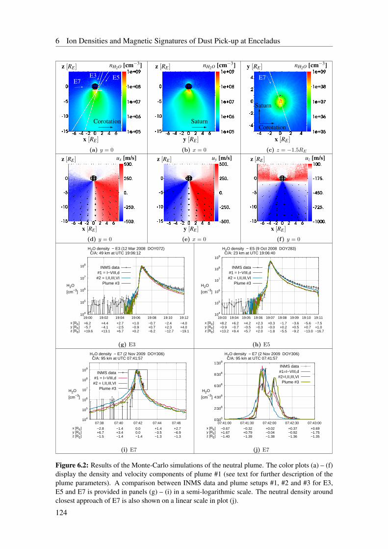
6 Ion Densities and Magnetic Signatures of Dust Pick-up at Enceladus
E3 E51E7
3Corotation
x [RE ]
z [RE ] nH2O [cm−3]
1
(a) y = 0
3Saturn
y [RE ]
z [RE ] nH2O [cm−3]
1
(b) x = 0
AAU
E7
3Corotation
3
Saturn
x [RE ]
y [RE ] nH2O [cm−3]
1
(c) z = −1.5RE
x [RE ]
z [RE ] ux [m/s]
1
(d) y = 0
y [RE ]
z [RE ] uy [m/s]
1
(e) x = 0
x [RE ]
z [RE ] uz [m/s]
1
(f) y = 0
104
105
106
107
108
19:00 19:02 19:04 19:06 19:08 19:10 19:12
H2O density − E3 (12 Mar 2008 DOY072) C/A: 49 km at UTC 19:06:12
x [RE]y [RE]z [RE]
+6.2−5.7+19.6
+4.4−4.1+13.1
+2.7−2.5+6.7
+1.0−0.9+0.2
−0.7+0.7−6.2
−2.4+2.3−12.7
−4.0+4.0−19.1
H2O
[cm−3]
INMS data#1 = I−VIII,d#2 = I,II,III,VI
Plume #3
(g) E3
104
105
106
107
108
109
19:03 19:04 19:05 19:06 19:07 19:08 19:09 19:10 19:11
H2O density − E5 (9 Oct 2008 DOY283) C/A: 23 km at UTC 19:06:40
x [RE]y [RE]z [RE]
+8.2−0.9+13.2
+6.2−0.7+9.4
+4.2−0.5+5.7
+2.3−0.3+2.0
+0.3−0.0−1.8
−1.7+0.2−5.5
−3.6+0.5−9.2
−5.6+0.7−13.0
−7.5+1.0−16.7
H2O
[cm−3]
INMS data#1 = I−VIII,d#2 = I,II,III,VI
Plume #3
(h) E5
104
105
106
107
108
109
07:38 07:40 07:42 07:44 07:46
H2O density − E7 (2 Nov 2009 DOY306) C/A: 95 km at UTC 07:41:57
x [RE]y [RE]z [RE]
−2.8+6.7−1.5
−1.4+3.4−1.4
0.00.0−1.4
+1.4−3.5−1.3
+2.7−6.9−1.3
H2O
[cm−3]
INMS data#1 = I−VIII,d#2 = I,II,III,VI
Plume #3
(i) E7
0⋅100
2⋅108
4⋅108
6⋅108
8⋅108
1⋅109
07:41:00 07:41:30 07:42:00 07:42:30 07:43:00
H2O density − E7 (2 Nov 2009 DOY306) C/A: 95 km at UTC 07:41:57
x [RE]y [RE]z [RE]
−0.67+1.67−1.40
−0.32+0.79−1.39
+0.02−0.04−1.38
+0.37−0.92−1.36
+0.69−1.75−1.35
H2O
[cm−3]
INMS data#1=I−VIII,d#2=I,II,III,VI
Plume #3
(j) E7
Figure 6.2: Results of the Monte-Carlo simulations of the neutral plume. The color plots (a) – (f)display the density and velocity components of plume #1 (see text for further description of theplume parameters). A comparison between INMS data and plume setups #1, #2 and #3 for E3,E5 and E7 is provided in panels (g) – (i) in a semi-logarithmic scale. The neutral density aroundclosest approach of E7 is also shown on a linear scale in plot (j).
124
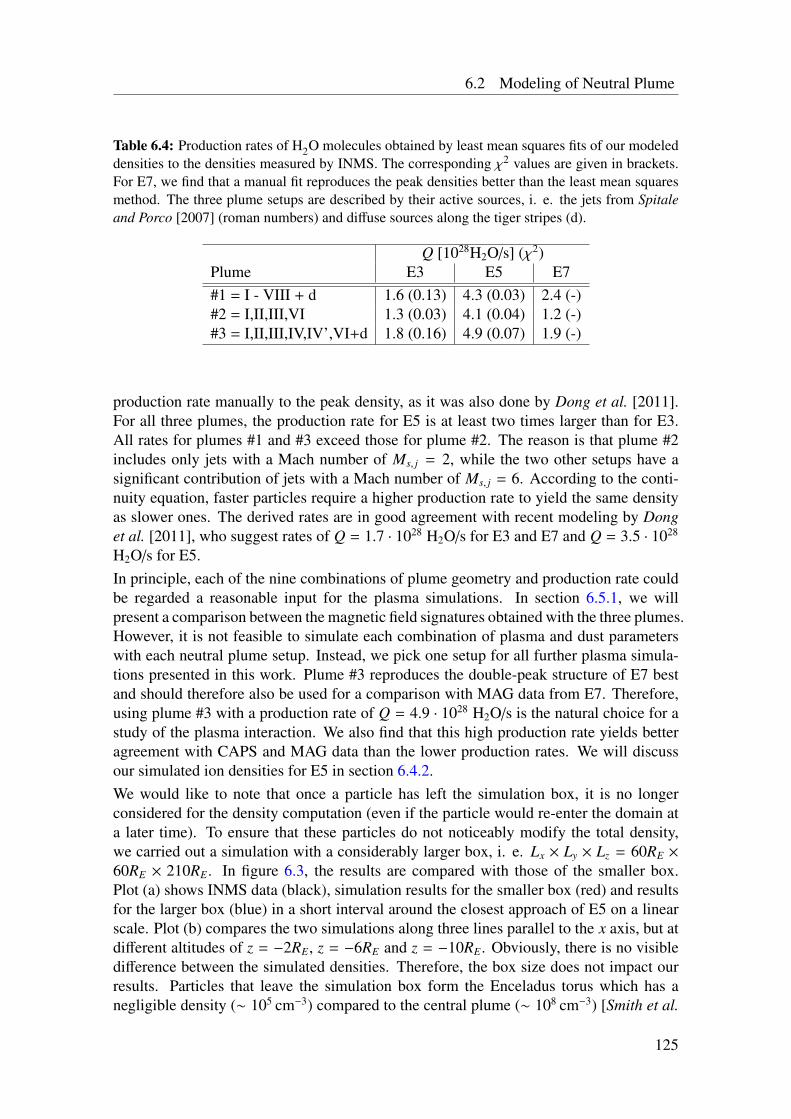
6.2 Modeling of Neutral Plume
Table 6.4: Production rates of H2O molecules obtained by least mean squares fits of our modeleddensities to the densities measured by INMS. The corresponding χ2 values are given in brackets.For E7, we find that a manual fit reproduces the peak densities better than the least mean squaresmethod. The three plume setups are described by their active sources, i. e. the jets from Spitaleand Porco [2007] (roman numbers) and diffuse sources along the tiger stripes (d).
Q [1028H2O/s] (χ2)Plume E3 E5 E7#1 = I - VIII + d 1.6 (0.13) 4.3 (0.03) 2.4 (-)#2 = I,II,III,VI 1.3 (0.03) 4.1 (0.04) 1.2 (-)#3 = I,II,III,IV,IV’,VI+d 1.8 (0.16) 4.9 (0.07) 1.9 (-)
production rate manually to the peak density, as it was also done by Dong et al. [2011].For all three plumes, the production rate for E5 is at least two times larger than for E3.All rates for plumes #1 and #3 exceed those for plume #2. The reason is that plume #2includes only jets with a Mach number of Ms, j = 2, while the two other setups have asignificant contribution of jets with a Mach number of Ms, j = 6. According to the conti-nuity equation, faster particles require a higher production rate to yield the same densityas slower ones. The derived rates are in good agreement with recent modeling by Donget al. [2011], who suggest rates of Q = 1.7 · 1028 H2O/s for E3 and E7 and Q = 3.5 · 1028
H2O/s for E5.In principle, each of the nine combinations of plume geometry and production rate couldbe regarded a reasonable input for the plasma simulations. In section 6.5.1, we willpresent a comparison between the magnetic field signatures obtained with the three plumes.However, it is not feasible to simulate each combination of plasma and dust parameterswith each neutral plume setup. Instead, we pick one setup for all further plasma simula-tions presented in this work. Plume #3 reproduces the double-peak structure of E7 bestand should therefore also be used for a comparison with MAG data from E7. Therefore,using plume #3 with a production rate of Q = 4.9 · 1028 H2O/s is the natural choice for astudy of the plasma interaction. We also find that this high production rate yields betteragreement with CAPS and MAG data than the lower production rates. We will discussour simulated ion densities for E5 in section 6.4.2.We would like to note that once a particle has left the simulation box, it is no longerconsidered for the density computation (even if the particle would re-enter the domain ata later time). To ensure that these particles do not noticeably modify the total density,we carried out a simulation with a considerably larger box, i. e. Lx × Ly × Lz = 60RE ×
60RE × 210RE. In figure 6.3, the results are compared with those of the smaller box.Plot (a) shows INMS data (black), simulation results for the smaller box (red) and resultsfor the larger box (blue) in a short interval around the closest approach of E5 on a linearscale. Plot (b) compares the two simulations along three lines parallel to the x axis, but atdifferent altitudes of z = −2RE, z = −6RE and z = −10RE. Obviously, there is no visibledifference between the simulated densities. Therefore, the box size does not impact ourresults. Particles that leave the simulation box form the Enceladus torus which has anegligible density (∼ 105 cm−3) compared to the central plume (∼ 108 cm−3) [Smith et al.
125
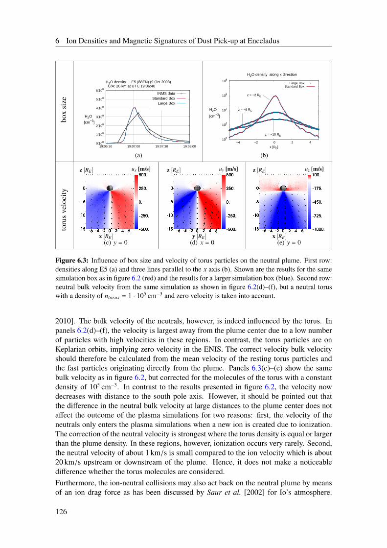
6 Ion Densities and Magnetic Signatures of Dust Pick-up at Enceladus
box
size
0⋅100
1⋅108
2⋅108
3⋅108
4⋅108
5⋅108
6⋅108
19:06:30 19:07:00 19:07:30 19:08:00
H2O density − E5 (88EN) (9 Oct 2008) C/A: 26 km at UTC 19:06:40
H2O
[cm−3]
INMS dataStandard Box
Large Box
(a)
105
106
107
108
109
−4 −2 0 2 4x [RE]
H2O
[cm−3]
H2O density along x direction
z = −2 RE
z = −6 RE
z = −10 RE
Large BoxStandard Box
(b)
toru
sve
loci
ty
x [RE ]
z [RE ] ux [m/s]
1
(c) y = 0y [RE ]
z [RE ] uy [m/s]
1
(d) x = 0x [RE ]
z [RE ] uz [m/s]
1
(e) y = 0
Figure 6.3: Influence of box size and velocity of torus particles on the neutral plume. First row:densities along E5 (a) and three lines parallel to the x axis (b). Shown are the results for the samesimulation box as in figure 6.2 (red) and the results for a larger simulation box (blue). Second row:neutral bulk velocity from the same simulation as shown in figure 6.2(d)–(f), but a neutral toruswith a density of ntorus = 1 · 105 cm−3 and zero velocity is taken into account.
2010]. The bulk velocity of the neutrals, however, is indeed influenced by the torus. Inpanels 6.2(d)–(f), the velocity is largest away from the plume center due to a low numberof particles with high velocities in these regions. In contrast, the torus particles are onKeplarian orbits, implying zero velocity in the ENIS. The correct velocity bulk velocityshould therefore be calculated from the mean velocity of the resting torus particles andthe fast particles originating directly from the plume. Panels 6.3(c)–(e) show the samebulk velocity as in figure 6.2, but corrected for the molecules of the torus with a constantdensity of 105 cm−3. In contrast to the results presented in figure 6.2, the velocity nowdecreases with distance to the south pole axis. However, it should be pointed out thatthe difference in the neutral bulk velocity at large distances to the plume center does notaffect the outcome of the plasma simulations for two reasons: first, the velocity of theneutrals only enters the plasma simulations when a new ion is created due to ionization.The correction of the neutral velocity is strongest where the torus density is equal or largerthan the plume density. In these regions, however, ionization occurs very rarely. Second,the neutral velocity of about 1 km/s is small compared to the ion velocity which is about20 km/s upstream or downstream of the plume. Hence, it does not make a noticeabledifference whether the torus molecules are considered.Furthermore, the ion-neutral collisions may also act back on the neutral plume by meansof an ion drag force as has been discussed by Saur et al. [2002] for Io’s atmosphere.
126
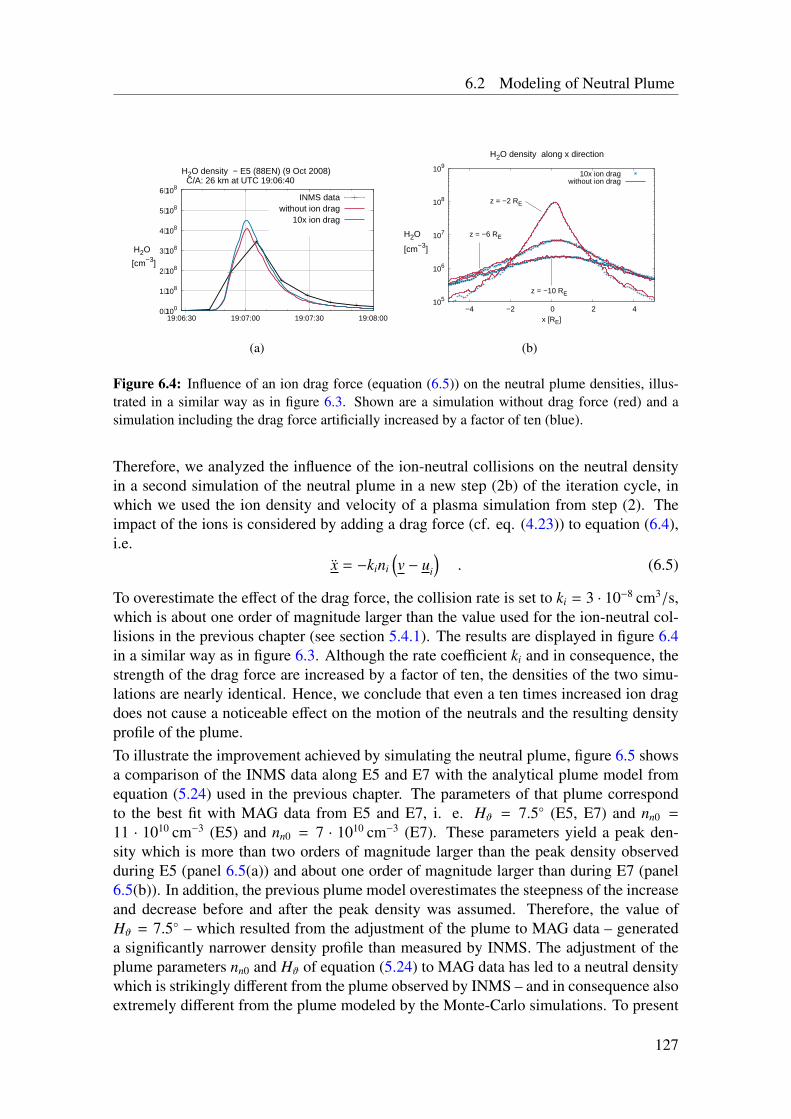
6.2 Modeling of Neutral Plume
0⋅100
1⋅108
2⋅108
3⋅108
4⋅108
5⋅108
6⋅108
19:06:30 19:07:00 19:07:30 19:08:00
H2O density − E5 (88EN) (9 Oct 2008) C/A: 26 km at UTC 19:06:40
H2O
[cm−3]
INMS datawithout ion drag
10x ion drag
(a)
105
106
107
108
109
−4 −2 0 2 4x [RE]
H2O
[cm−3]
H2O density along x direction
z = −2 RE
z = −6 RE
z = −10 RE
10x ion dragwithout ion drag
(b)
Figure 6.4: Influence of an ion drag force (equation (6.5)) on the neutral plume densities, illus-trated in a similar way as in figure 6.3. Shown are a simulation without drag force (red) and asimulation including the drag force artificially increased by a factor of ten (blue).
Therefore, we analyzed the influence of the ion-neutral collisions on the neutral densityin a second simulation of the neutral plume in a new step (2b) of the iteration cycle, inwhich we used the ion density and velocity of a plasma simulation from step (2). Theimpact of the ions is considered by adding a drag force (cf. eq. (4.23)) to equation (6.4),i.e.
x = −kini
(v − ui
). (6.5)
To overestimate the effect of the drag force, the collision rate is set to ki = 3 · 10−8 cm3/s,which is about one order of magnitude larger than the value used for the ion-neutral col-lisions in the previous chapter (see section 5.4.1). The results are displayed in figure 6.4in a similar way as in figure 6.3. Although the rate coefficient ki and in consequence, thestrength of the drag force are increased by a factor of ten, the densities of the two simu-lations are nearly identical. Hence, we conclude that even a ten times increased ion dragdoes not cause a noticeable effect on the motion of the neutrals and the resulting densityprofile of the plume.To illustrate the improvement achieved by simulating the neutral plume, figure 6.5 showsa comparison of the INMS data along E5 and E7 with the analytical plume model fromequation (5.24) used in the previous chapter. The parameters of that plume correspondto the best fit with MAG data from E5 and E7, i. e. Hϑ = 7.5 (E5, E7) and nn0 =
11 · 1010 cm−3 (E5) and nn0 = 7 · 1010 cm−3 (E7). These parameters yield a peak den-sity which is more than two orders of magnitude larger than the peak density observedduring E5 (panel 6.5(a)) and about one order of magnitude larger than during E7 (panel6.5(b)). In addition, the previous plume model overestimates the steepness of the increaseand decrease before and after the peak density was assumed. Therefore, the value ofHϑ = 7.5 – which resulted from the adjustment of the plume to MAG data – generateda significantly narrower density profile than measured by INMS. The adjustment of theplume parameters nn0 and Hϑ of equation (5.24) to MAG data has led to a neutral densitywhich is strikingly different from the plume observed by INMS – and in consequence alsoextremely different from the plume modeled by the Monte-Carlo simulations. To present
127
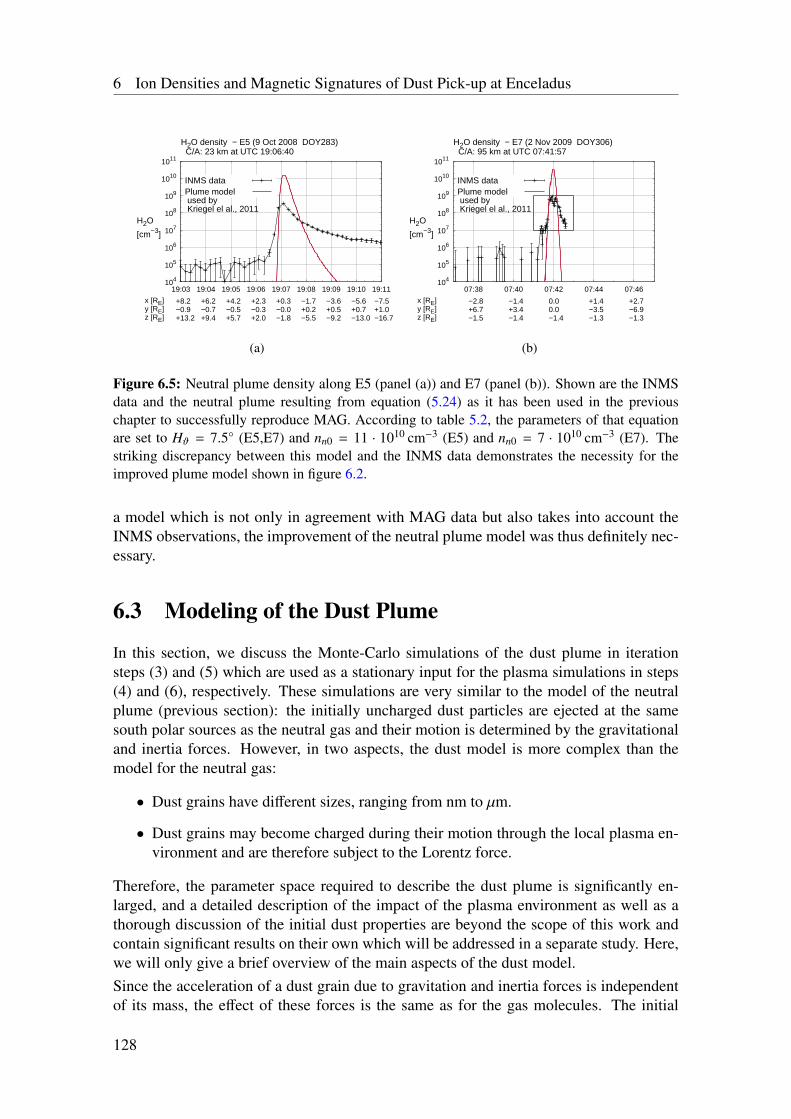
6 Ion Densities and Magnetic Signatures of Dust Pick-up at Enceladus
104
105
106
107
108
109
1010
1011
19:03 19:04 19:05 19:06 19:07 19:08 19:09 19:10 19:11
H2O density − E5 (9 Oct 2008 DOY283) C/A: 23 km at UTC 19:06:40
x [RE]y [RE]z [RE]
+8.2−0.9+13.2
+6.2−0.7+9.4
+4.2−0.5+5.7
+2.3−0.3+2.0
+0.3−0.0−1.8
−1.7+0.2−5.5
−3.6+0.5−9.2
−5.6+0.7−13.0
−7.5+1.0−16.7
H2O
[cm−3]
INMS dataPlume model used by Kriegel el al., 2011
(a)
104
105
106
107
108
109
1010
1011
07:38 07:40 07:42 07:44 07:46
H2O density − E7 (2 Nov 2009 DOY306) C/A: 95 km at UTC 07:41:57
x [RE]y [RE]z [RE]
−2.8+6.7−1.5
−1.4+3.4−1.4
0.00.0−1.4
+1.4−3.5−1.3
+2.7−6.9−1.3
H2O
[cm−3]
INMS dataPlume model used by Kriegel el al., 2011
(b)
Figure 6.5: Neutral plume density along E5 (panel (a)) and E7 (panel (b)). Shown are the INMSdata and the neutral plume resulting from equation (5.24) as it has been used in the previouschapter to successfully reproduce MAG. According to table 5.2, the parameters of that equationare set to Hϑ = 7.5 (E5,E7) and nn0 = 11 · 1010 cm−3 (E5) and nn0 = 7 · 1010 cm−3 (E7). Thestriking discrepancy between this model and the INMS data demonstrates the necessity for theimproved plume model shown in figure 6.2.
a model which is not only in agreement with MAG data but also takes into account theINMS observations, the improvement of the neutral plume model was thus definitely nec-essary.
6.3 Modeling of the Dust Plume
In this section, we discuss the Monte-Carlo simulations of the dust plume in iterationsteps (3) and (5) which are used as a stationary input for the plasma simulations in steps(4) and (6), respectively. These simulations are very similar to the model of the neutralplume (previous section): the initially uncharged dust particles are ejected at the samesouth polar sources as the neutral gas and their motion is determined by the gravitationaland inertia forces. However, in two aspects, the dust model is more complex than themodel for the neutral gas:
• Dust grains have different sizes, ranging from nm to µm.
• Dust grains may become charged during their motion through the local plasma en-vironment and are therefore subject to the Lorentz force.
Therefore, the parameter space required to describe the dust plume is significantly en-larged, and a detailed description of the impact of the plasma environment as well as athorough discussion of the initial dust properties are beyond the scope of this work andcontain significant results on their own which will be addressed in a separate study. Here,we will only give a brief overview of the main aspects of the dust model.Since the acceleration of a dust grain due to gravitation and inertia forces is independentof its mass, the effect of these forces is the same as for the gas molecules. The initial
128
6.3 Modeling of the Dust Plume
velocity uD0 of the dust grains, however, is probably generated by collisions with theambient gas flow and is therefore a function of the grain size. This is considered byapplying the velocity-size distribution from Postberg et al. [2011] (equation S11), whomodeled the composition of the grains to match the CDA data. In their model, nanograinshave an initial velocity very close to that of the gas molecules (uD0(R ∼ nm) ≈ ugas), butlarger grains may be significantly slower, e. g. a grain of radius R = 1 µm has an averagevelocity of about uD0(R = 1 µm) = 0.4ugas when leaving the surface of Enceladus.To analyze the magnetic field signatures of the dust plume, we apply three different param-eter sets for the initial conditions of the dust grains. The first setup comprises only the dif-fuse tiger stripe sources with uD0 = 660 m/s, while the second setup includes only the jetlocations and associated directions from Spitale and Porco [2007] with uD0 = 2000 m/s.These choices correspond to a temperature of 180 K and sonic Mach numbers of the gasof Ms = 2 and Ms = 6, respectively. In the following, the model dust plumes resultingfrom these initial parameters will be referred to as ’diffuse dust (plume)’ and ’jet dust(plume)’. The two setups have been chosen to be consistent with the finding of Postberget al. [2011] that the slow (salt-rich) particles originate from the diffuse sources while thefaster (salt-poor) grains originate from the discrete jets. In their model, the grains leavethe tiger stripe sources with a mean ejection angle of ψ = 35 with respect to the surfacenormal, while this angle is ψ = 15 for the jet sources. To account for these angles, weassume that the grains acquire an additional random velocity component correspondingto a Gaussian distribution with a standard deviation of σ = 500 m/s. In cases with onlyinterest in the general effect of the dust we apply a mixture of the two former setups andconsider both source types (default dust). Each jet source is assigned a four times highersource rate. In addition, we will employ an analytical model of the dust charge densitysimilar to the one used in the simulations of the previous chapter (see section 5.4.3),
ξnD(x) = ξnd0RE
r′exp
(−ϑ′2
H2ϑ
)exp
(RE − r′
Hd
). (6.6)
The prime indicates that r′ and ϑ′ are the radial distance and the polar angle with respectto the south pole, not the center of Enceladus. Although eq. (6.6) diverges at the southpole from the analytical point of view, it does not do so in our simulation due to the finitegrid resolution, where no mesh node is located exactly at r′ = 0. We set ξnd0 = 750 cm−3,Hϑ = 20 and Hd = 948 km. We would like to emphasize that we do not intend to regardthis profile as realistic or physically justified, yet, a comparison of this simple profile withthe results from the Monte-Carlo simulations allows interesting conclusions on the impactof the dust on the magnetic field in section 6.5.CDA measurements show that the size distribution of grains larger than 1 µm follows apower law according to dnd ∼ R−µdR [Kempf et al. 2010]. The dust charge density ξnD,that is the number of electrons absorbed per volume by the dust grains is then obtainedfrom integration over the size distribution multiplied by the charge qd(R) carried by agrain of a certain size R. Thus we get
ξnD ∼
Rmax∫Rmin
qd(R)Rµ
dR . (6.7)
129
6 Ion Densities and Magnetic Signatures of Dust Pick-up at Enceladus
The lower and upper cutoffs of our size distribution are set to Rmin = 1 nm and Rmax =
5 µm, respectively. Modeling of the dust formation by Schmidt et al. [2008] suggests thatthe slope of the logarithmic size distribution may not be constant within the whole rangeof sizes, but µ is a function of the grain radius, µ = µ(R). In our Monte-Carlo simulationsof the dust plume, we therefore use a piecewise constant µ(R):
µ(R) =
7 ; 1 nm ≤ R < 2 nm−5 ; 2 nm ≤ R < 200 nm−4 ; 200 nm ≤ R < 5 µm
. (6.8)
The magnitude of the dust density is mainly controlled by the mass production rate of thedust which is set to
Md =
0.5 kg/s ; 1 nm ≤ R < 2 nm7.7 kg/s ; 2 nm ≤ R < 200 nm8.0 kg/s ; 200 nm ≤ R < 5 µm
. (6.9)
On the one hand, the values for grains larger than R = 200 nm are adjusted to modeling ofCDA data, e.g. the mass production rate has been adjusted to CDA measurements alongthe E2 flyby [Kempf et al. 2010] and to the peak density seen along E7 [J. Schmidt; priv.comm.]. The slope of µ = −4 is in agreement with the model by Postberg et al. [2011].On the other hand, the parameters of the dust with 0.5 nm ≤ R < 2 nm are chosen tomatch the CAPS/ELS nanograin observations along E3 and E5 presented by Hill et al.[2012]. From figures 6 and 7 in that work, the slope can be estimated to be approximatelyµ ≈ 7. As will be discussed by Meier et al., in preparation, the value of Md = 0.5 kg/sfor R < 2 nm is a lower limit derived from the CAPS nanograin densities. The values for2 nm ≤ R < 200 nm are then obtained by assuming a continuous size distribution.Of course, the real parameters of the nanograin size distribution might be different fromour values. However, with the reasonable constraints that first, the slope of the size dis-tribution is positive for the nanograins and second, the total mass production rate of thedust must not get too large (we assume Md,total < 50 kg/s), the peak of any size distri-bution is located at radii smaller than 3 nm and thus, most of the dust particles are smallnanograins. For our size distribution, even more than 99% of the grains are smaller than10 nm.The grains are charged and discharged dynamically during their motion according to
dqd(R)dt
= Ie + Ii + Isec + Iph . (6.10)
The currents on the right-hand side of equation (6.10) are the local electron and ion collec-tion currents Ie and Ii, the secondary electron current Isec and the photoionization currentIph (see e. g. Shukla and Mamun [2002]). A major advantage of our iterative simulationtechnique is that these currents and the maximum number of available ”free” electronsare constrained by the realistic plasma environment from the hybrid simulations.We would like to note that many of the nanograins do not attain their equilibrium chargewhile being located within the central plume. Field emission limits the charge of grains
130
6.4 Results I: Plasma Densities
smaller than 2 nm to a single elementary charge [Hill et al. 2012]. In contrast, the equi-librium charge of larger grains is proportional to their radius [Shukla and Mamun 2002].Although the nanograins are not in equilibrium, the dust charge density resulting fromall nanograins within a certain volume reaches a steady state. A consequence of the sizedistribution defined by equations (6.8) and (6.9) is that 99% of the equilibrium chargedensity is carried by grains smaller than 10 nm.For singly-charged nanograins of R = 2 nm and a corresponding mass m = 110 mH2O, theacceleration by the Lorentz force FL in the upstream plasma dominates the gravitationalforce of Saturn (FG) at 3.95RS by about two orders of magnitude (FL/m ∼ 101 m/s2 vs.FG/m ∼ 10−1 m/s2 ). The electromagnetic fields are therefore crucial for the motionof the nanograins and the shape of the charged dust plume. We would like to note thatour model in principle also allows for positively charged nanograins. As they are clearlyoutnumbered by the negatively charged particles, the positive nanograins are not visiblein the total dust charge density.The resulting spatial distribution of the dust charge density will be shown in the discussionof the plasma densities (see section 6.4).
6.4 Results I: Plasma Densities
We commence the discussion of our results with the densities of the various ion speciesand the charged dust. For the macroscopic scales (∼ km) we discuss here, these densitiesare related by the quasi-neutrality condition∑
α
nα = ni = ne + ξnD , (6.11)
where nα denotes the density of the ion species α with α = H+,O+,OH+,H2O+,H3O+,ni is the total ion density, ne the electron density and ξnD the number of electrons absorbedby the dust grains per volume. First, we discuss the effect of the ion-neutral chemistry onthe relative abundances nα/ni of the various ion species. Second, we present our resultsfor the total ion density ni in the context of the Cassini observations. Finally, we describethe dust plume resulting from the Monte-Carlo simulations for different initial conditionsof the dust.We would like to note that all results presented in the following sections (6.4 and 6.5) areobtained from step (6) of our iteration scheme. If not stated otherwise, the simulations arebased on neutral plume #3 with a production rate of Q = 4.9 · 1028 H2O/s (cf. section 6.2)and the default dust plume which considers diffuse and jet dust sources (see section 6.3).
6.4.1 Ion Composition
As described in section 6.1.2, the upstream plasma composition is set to 10% protonsand 22.5% of each of the four water group ion species. Due to ion-neutral reactions andionization in the plume, these relative abundances change. Our simulation results for therelative abundances nα/ni of the different ion species are shown in panels (a)–(e) of figure6.6. As can be seen in plots (a), (b) and (c), the relative abundances of H+, O+ and OH+
131
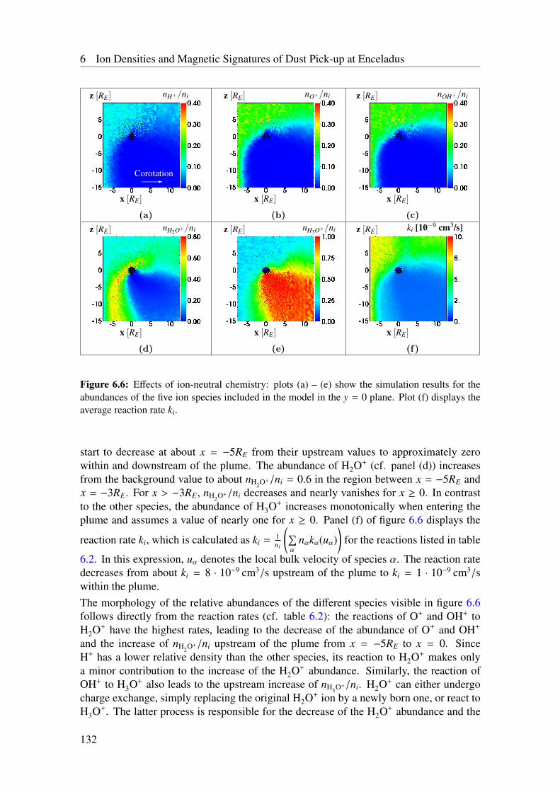
6 Ion Densities and Magnetic Signatures of Dust Pick-up at Enceladus
3Corotation
x [RE ]
z [RE ] nH+/ni
1
(a)
x [RE ]
z [RE ] nO+/ni
1
(b)
x [RE ]
z [RE ] nOH+/ni
1
(c)
x [RE ]
z [RE ] nH2O+/ni
1
(d)
x [RE ]
z [RE ] nH3O+/ni
1
(e)
x [RE ]
z [RE ] ki [10−9 cm3/s]
1
(f)
Figure 6.6: Effects of ion-neutral chemistry: plots (a) – (e) show the simulation results for theabundances of the five ion species included in the model in the y = 0 plane. Plot (f) displays theaverage reaction rate ki.
start to decrease at about x = −5RE from their upstream values to approximately zerowithin and downstream of the plume. The abundance of H2O+ (cf. panel (d)) increasesfrom the background value to about nH2O+/ni = 0.6 in the region between x = −5RE andx = −3RE. For x > −3RE, nH2O+/ni decreases and nearly vanishes for x ≥ 0. In contrastto the other species, the abundance of H3O+ increases monotonically when entering theplume and assumes a value of nearly one for x ≥ 0. Panel (f) of figure 6.6 displays the
reaction rate ki, which is calculated as ki = 1ni
(∑α
nαkα(uα))
for the reactions listed in table
6.2. In this expression, uα denotes the local bulk velocity of species α. The reaction ratedecreases from about ki = 8 · 10−9 cm3/s upstream of the plume to ki = 1 · 10−9 cm3/swithin the plume.The morphology of the relative abundances of the different species visible in figure 6.6follows directly from the reaction rates (cf. table 6.2): the reactions of O+ and OH+ toH2O+ have the highest rates, leading to the decrease of the abundance of O+ and OH+
and the increase of nH2O+/ni upstream of the plume from x = −5RE to x = 0. SinceH+ has a lower relative density than the other species, its reaction to H2O+ makes onlya minor contribution to the increase of the H2O+ abundance. Similarly, the reaction ofOH+ to H3O+ also leads to the upstream increase of nH3O+/ni. H2O+ can either undergocharge exchange, simply replacing the original H2O+ ion by a newly born one, or react toH3O+. The latter process is responsible for the decrease of the H2O+ abundance and the
132
6.4 Results I: Plasma Densities
increase of nH3O+/ni. When approaching x = 0 from upstream, these reactions occur sofrequently that nearly all H2O+ ions are converted to H3O+. Finally, H3O+ does not reactwith water at these energies and thus, it undergoes only elastic collisions with the neutralH2O molecules, yielding no change in its abundance. The high abundance of H3O+ withinthe center of the plume also explains the spatial profile of the reaction rate: ki is calculatedas an average over the different rates of the ion species. Within the plume, however, theaverage is dominated by the collisions of H3O+ which possess one of the smallest rates inthe reaction scheme: ki ≈ kH3O+ = 1.02 · 10−9 cm3/s.The ion-neutral chemistry relevant for Enceladus’ plasma interaction can therefore besummarized as follows: (1) all reactions of the upstream ions with H2O produce eitherH2O+ or H3O+, (2) H2O+ also reacts to H3O+, (3) H3O+ does not react any more. There-fore, the reaction chain ends up in the production of H3O+ which is the predominant ionspecies in the plume (abundance of nH3O+/ni ≈ 1). This finding is in agreement withINMS data [Cravens et al. 2009].We would like to point out that the velocity of the plasma has only a minor impact on thetotal reaction rate within the plume, since the rate of H3O+ is independent of the velocity(see appendix A). It is also interesting to note that the production of new ions within theplume by photo- and electron impact ionization has a negligible impact on the abundancesof the different species. Although these processes produce primarily H2O+, these newlyborn ions then quickly react to H3O+ and do not yield a noticeable abundance of H2O+.
6.4.2 Ion Densities
Before presenting our simulation results for the total ion density ni, we will derive ananalytical estimate of the maximum ion density in the plume based on ionization of aneutral plume model.In stationary state, the continuity equation for the ions reads
∂x · (niui) = νionH2O(x) , (6.12)
where we have neglected the contribution of the upstream plasma and loss terms arisingfrom recombination. To specify ui, we assume that in the center of the plume, ion-neutralcollisions occur so frequently that the ions are not accelerated to speeds above the velocityof the neutrals. This is in agreement with CAPS observations of flow stagnation [Tokaret al. 2009] and our previous simulation results. Furthermore, we have shown in section6.2 that the neutral bulk velocity un is mainly directed radially away from the south polarsources, i. e. un = un er with the radial unit vector er. The neutral density above thesources is approximated by the geometrical decrease of the density according to
nH2O(r) = nn0
(RE
r
)2
. (6.13)
According to the discussion in section 6.1.3, we assume νio to be constant. Setting ui =
uner and un = const, it is then possible to integrate eq. (6.12) in spherical coordinates,yielding
133
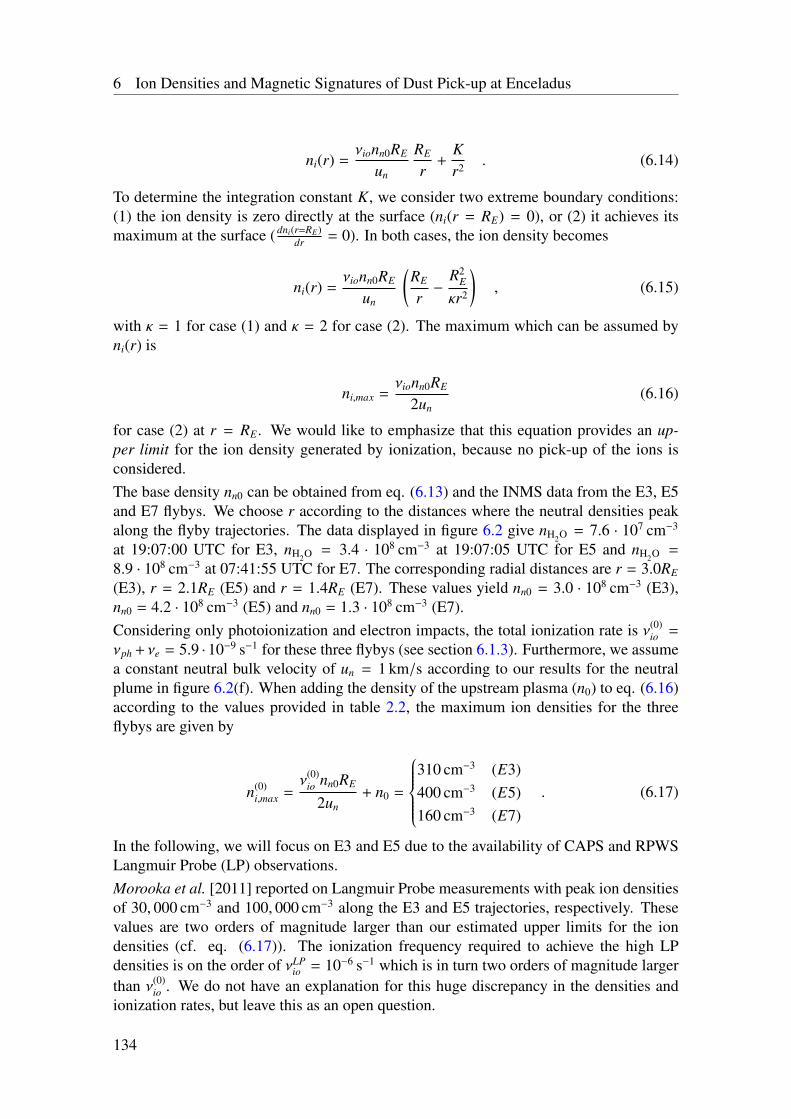
6 Ion Densities and Magnetic Signatures of Dust Pick-up at Enceladus
ni(r) =νionn0RE
un
RE
r+
Kr2 . (6.14)
To determine the integration constant K, we consider two extreme boundary conditions:(1) the ion density is zero directly at the surface (ni(r = RE) = 0), or (2) it achieves itsmaximum at the surface (dni(r=RE)
dr = 0). In both cases, the ion density becomes
ni(r) =νionn0RE
un
(RE
r−
R2E
κr2
), (6.15)
with κ = 1 for case (1) and κ = 2 for case (2). The maximum which can be assumed byni(r) is
ni,max =νionn0RE
2un(6.16)
for case (2) at r = RE. We would like to emphasize that this equation provides an up-per limit for the ion density generated by ionization, because no pick-up of the ions isconsidered.The base density nn0 can be obtained from eq. (6.13) and the INMS data from the E3, E5and E7 flybys. We choose r according to the distances where the neutral densities peakalong the flyby trajectories. The data displayed in figure 6.2 give nH2O = 7.6 · 107 cm−3
at 19:07:00 UTC for E3, nH2O = 3.4 · 108 cm−3 at 19:07:05 UTC for E5 and nH2O =
8.9 · 108 cm−3 at 07:41:55 UTC for E7. The corresponding radial distances are r = 3.0RE
(E3), r = 2.1RE (E5) and r = 1.4RE (E7). These values yield nn0 = 3.0 · 108 cm−3 (E3),nn0 = 4.2 · 108 cm−3 (E5) and nn0 = 1.3 · 108 cm−3 (E7).Considering only photoionization and electron impacts, the total ionization rate is ν(0)
io =
νph + νe = 5.9 · 10−9 s−1 for these three flybys (see section 6.1.3). Furthermore, we assumea constant neutral bulk velocity of un = 1 km/s according to our results for the neutralplume in figure 6.2(f). When adding the density of the upstream plasma (n0) to eq. (6.16)according to the values provided in table 2.2, the maximum ion densities for the threeflybys are given by
n(0)i,max =
ν(0)io nn0RE
2un+ n0 =
310 cm−3 (E3)400 cm−3 (E5)160 cm−3 (E7)
. (6.17)
In the following, we will focus on E3 and E5 due to the availability of CAPS and RPWSLangmuir Probe (LP) observations.Morooka et al. [2011] reported on Langmuir Probe measurements with peak ion densitiesof 30, 000 cm−3 and 100, 000 cm−3 along the E3 and E5 trajectories, respectively. Thesevalues are two orders of magnitude larger than our estimated upper limits for the iondensities (cf. eq. (6.17)). The ionization frequency required to achieve the high LPdensities is on the order of νLP
io = 10−6 s−1 which is in turn two orders of magnitude largerthan ν(0)
io . We do not have an explanation for this huge discrepancy in the densities andionization rates, but leave this as an open question.
134
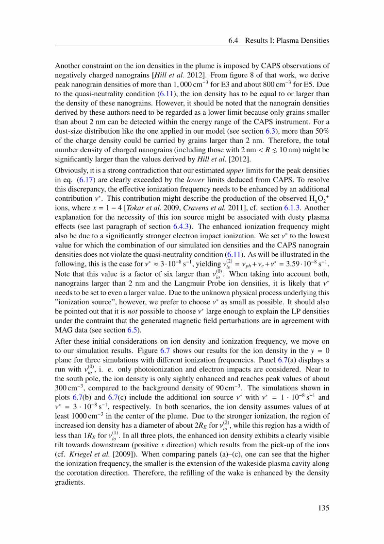
6.4 Results I: Plasma Densities
Another constraint on the ion densities in the plume is imposed by CAPS observations ofnegatively charged nanograins [Hill et al. 2012]. From figure 8 of that work, we derivepeak nanograin densities of more than 1, 000 cm−3 for E3 and about 800 cm−3 for E5. Dueto the quasi-neutrality condition (6.11), the ion density has to be equal to or larger thanthe density of these nanograins. However, it should be noted that the nanograin densitiesderived by these authors need to be regarded as a lower limit because only grains smallerthan about 2 nm can be detected within the energy range of the CAPS instrument. For adust-size distribution like the one applied in our model (see section 6.3), more than 50%of the charge density could be carried by grains larger than 2 nm. Therefore, the totalnumber density of charged nanograins (including those with 2 nm < R . 10 nm) might besignificantly larger than the values derived by Hill et al. [2012].Obviously, it is a strong contradiction that our estimated upper limits for the peak densitiesin eq. (6.17) are clearly exceeded by the lower limits deduced from CAPS. To resolvethis discrepancy, the effective ionization frequency needs to be enhanced by an additionalcontribution ν∗. This contribution might describe the production of the observed HxO2
+
ions, where x = 1 − 4 [Tokar et al. 2009, Cravens et al. 2011], cf. section 6.1.3. Anotherexplanation for the necessity of this ion source might be associated with dusty plasmaeffects (see last paragraph of section 6.4.3). The enhanced ionization frequency mightalso be due to a significantly stronger electron impact ionization. We set ν∗ to the lowestvalue for which the combination of our simulated ion densities and the CAPS nanograindensities does not violate the quasi-neutrality condition (6.11). As will be illustrated in thefollowing, this is the case for ν∗ ≈ 3 ·10−8 s−1, yielding ν(2)
io = νph +νe +ν∗ = 3.59 ·10−8 s−1.Note that this value is a factor of six larger than ν(0)
io . When taking into account both,nanograins larger than 2 nm and the Langmuir Probe ion densities, it is likely that ν∗
needs to be set to even a larger value. Due to the unknown physical process underlying this”ionization source”, however, we prefer to choose ν∗ as small as possible. It should alsobe pointed out that it is not possible to choose ν∗ large enough to explain the LP densitiesunder the contraint that the generated magnetic field perturbations are in agreement withMAG data (see section 6.5).After these initial considerations on ion density and ionization frequency, we move onto our simulation results. Figure 6.7 shows our results for the ion density in the y = 0plane for three simulations with different ionization frequencies. Panel 6.7(a) displays arun with ν(0)
io , i. e. only photoionization and electron impacts are considered. Near tothe south pole, the ion density is only sightly enhanced and reaches peak values of about300 cm−3, compared to the background density of 90 cm−3. The simulations shown inplots 6.7(b) and 6.7(c) include the additional ion source ν∗ with ν∗ = 1 · 10−8 s−1 andν∗ = 3 · 10−8 s−1, respectively. In both scenarios, the ion density assumes values of atleast 1000 cm−3 in the center of the plume. Due to the stronger ionization, the region ofincreased ion density has a diameter of about 2RE for ν(2)
io , while this region has a width ofless than 1RE for ν(1)
io . In all three plots, the enhanced ion density exhibits a clearly visibletilt towards downstream (positive x direction) which results from the pick-up of the ions(cf. Kriegel et al. [2009]). When comparing panels (a)–(c), one can see that the higherthe ionization frequency, the smaller is the extension of the wakeside plasma cavity alongthe corotation direction. Therefore, the refilling of the wake is enhanced by the densitygradients.
135
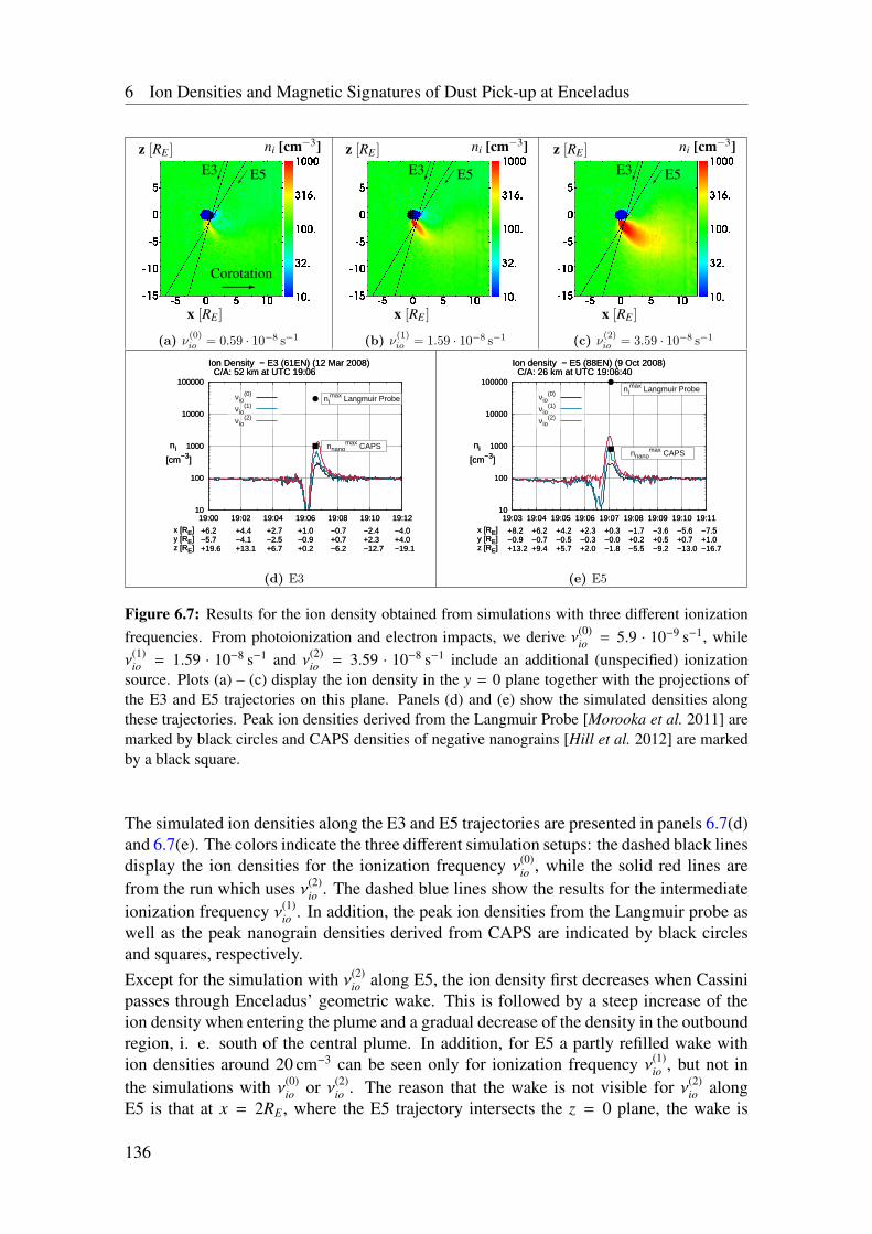
6 Ion Densities and Magnetic Signatures of Dust Pick-up at Enceladus
E3 E5
3Corotation
x [RE ]
z [RE ] ni [cm−3]
1
(a) ν(0)io = 0.59 · 10−8 s−1
E3 E5
x [RE ]
z [RE ] ni [cm−3]
1
(b) ν(1)io = 1.59 · 10−8 s−1
E3 E5
x [RE ]
z [RE ] ni [cm−3]
1
(c) ν(2)io = 3.59 · 10−8 s−1
10
100
1000
10000
100000
19:00 19:02 19:04 19:06 19:08 19:10 19:12
Ion Density − E3 (61EN) (12 Mar 2008) C/A: 52 km at UTC 19:06
x [RE]y [RE]z [RE]
+6.2−5.7+19.6
+4.4−4.1+13.1
+2.7−2.5+6.7
+1.0−0.9+0.2
−0.7+0.7−6.2
−2.4+2.3−12.7
−4.0+4.0−19.1
ni
[cm−3]
νio(0)
νio(1)
νio(2)
10
100
1000
10000
100000
19:00 19:02 19:04 19:06 19:08 19:10 19:12
Ion Density − E3 (61EN) (12 Mar 2008) C/A: 52 km at UTC 19:06
x [RE]y [RE]z [RE]
+6.2−5.7+19.6
+4.4−4.1+13.1
+2.7−2.5+6.7
+1.0−0.9+0.2
−0.7+0.7−6.2
−2.4+2.3−12.7
−4.0+4.0−19.1
ni
[cm−3]
nimax Langmuir Probe
nnanomax CAPS
(d) E3
10
100
1000
10000
100000
19:03 19:04 19:05 19:06 19:07 19:08 19:09 19:10 19:11
Ion density − E5 (88EN) (9 Oct 2008) C/A: 26 km at UTC 19:06:40
x [RE]y [RE]z [RE]
+8.2−0.9+13.2
+6.2−0.7+9.4
+4.2−0.5+5.7
+2.3−0.3+2.0
+0.3−0.0−1.8
−1.7+0.2−5.5
−3.6+0.5−9.2
−5.6+0.7−13.0
−7.5+1.0−16.7
ni
[cm−3]
νio(0)
νio(1)
νio(2)
10
100
1000
10000
100000
19:03 19:04 19:05 19:06 19:07 19:08 19:09 19:10 19:11
Ion density − E5 (88EN) (9 Oct 2008) C/A: 26 km at UTC 19:06:40
x [RE]y [RE]z [RE]
+8.2−0.9+13.2
+6.2−0.7+9.4
+4.2−0.5+5.7
+2.3−0.3+2.0
+0.3−0.0−1.8
−1.7+0.2−5.5
−3.6+0.5−9.2
−5.6+0.7−13.0
−7.5+1.0−16.7
ni
[cm−3]
nimax Langmuir Probe
nnanomax CAPS
(e) E5
Figure 6.7: Results for the ion density obtained from simulations with three different ionizationfrequencies. From photoionization and electron impacts, we derive ν(0)
io = 5.9 · 10−9 s−1, whileν(1)
io = 1.59 · 10−8 s−1 and ν(2)io = 3.59 · 10−8 s−1 include an additional (unspecified) ionization
source. Plots (a) – (c) display the ion density in the y = 0 plane together with the projections ofthe E3 and E5 trajectories on this plane. Panels (d) and (e) show the simulated densities alongthese trajectories. Peak ion densities derived from the Langmuir Probe [Morooka et al. 2011] aremarked by black circles and CAPS densities of negative nanograins [Hill et al. 2012] are markedby a black square.
The simulated ion densities along the E3 and E5 trajectories are presented in panels 6.7(d)and 6.7(e). The colors indicate the three different simulation setups: the dashed black linesdisplay the ion densities for the ionization frequency ν(0)
io , while the solid red lines arefrom the run which uses ν(2)
io . The dashed blue lines show the results for the intermediateionization frequency ν(1)
io . In addition, the peak ion densities from the Langmuir probe aswell as the peak nanograin densities derived from CAPS are indicated by black circlesand squares, respectively.Except for the simulation with ν(2)
io along E5, the ion density first decreases when Cassinipasses through Enceladus’ geometric wake. This is followed by a steep increase of theion density when entering the plume and a gradual decrease of the density in the outboundregion, i. e. south of the central plume. In addition, for E5 a partly refilled wake withion densities around 20 cm−3 can be seen only for ionization frequency ν(1)
io , but not inthe simulations with ν(0)
io or ν(2)io . The reason that the wake is not visible for ν(2)
io alongE5 is that at x = 2RE, where the E5 trajectory intersects the z = 0 plane, the wake is
136
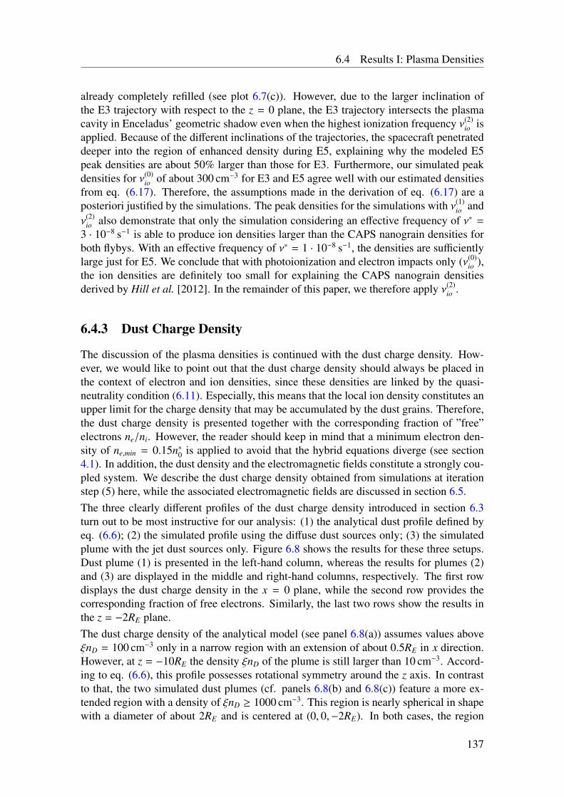
6.4 Results I: Plasma Densities
already completely refilled (see plot 6.7(c)). However, due to the larger inclination ofthe E3 trajectory with respect to the z = 0 plane, the E3 trajectory intersects the plasmacavity in Enceladus’ geometric shadow even when the highest ionization frequency ν(2)
io isapplied. Because of the different inclinations of the trajectories, the spacecraft penetrateddeeper into the region of enhanced density during E5, explaining why the modeled E5peak densities are about 50% larger than those for E3. Furthermore, our simulated peakdensities for ν(0)
io of about 300 cm−3 for E3 and E5 agree well with our estimated densitiesfrom eq. (6.17). Therefore, the assumptions made in the derivation of eq. (6.17) are aposteriori justified by the simulations. The peak densities for the simulations with ν(1)
io andν(2)
io also demonstrate that only the simulation considering an effective frequency of ν∗ =
3 · 10−8 s−1 is able to produce ion densities larger than the CAPS nanograin densities forboth flybys. With an effective frequency of ν∗ = 1 · 10−8 s−1, the densities are sufficientlylarge just for E5. We conclude that with photoionization and electron impacts only (ν(0)
io ),the ion densities are definitely too small for explaining the CAPS nanograin densitiesderived by Hill et al. [2012]. In the remainder of this paper, we therefore apply ν(2)
io .
6.4.3 Dust Charge Density
The discussion of the plasma densities is continued with the dust charge density. How-ever, we would like to point out that the dust charge density should always be placed inthe context of electron and ion densities, since these densities are linked by the quasi-neutrality condition (6.11). Especially, this means that the local ion density constitutes anupper limit for the charge density that may be accumulated by the dust grains. Therefore,the dust charge density is presented together with the corresponding fraction of ”free”electrons ne/ni. However, the reader should keep in mind that a minimum electron den-sity of ne,min = 0.15n∗0 is applied to avoid that the hybrid equations diverge (see section4.1). In addition, the dust density and the electromagnetic fields constitute a strongly cou-pled system. We describe the dust charge density obtained from simulations at iterationstep (5) here, while the associated electromagnetic fields are discussed in section 6.5.The three clearly different profiles of the dust charge density introduced in section 6.3turn out to be most instructive for our analysis: (1) the analytical dust profile defined byeq. (6.6); (2) the simulated profile using the diffuse dust sources only; (3) the simulatedplume with the jet dust sources only. Figure 6.8 shows the results for these three setups.Dust plume (1) is presented in the left-hand column, whereas the results for plumes (2)and (3) are displayed in the middle and right-hand columns, respectively. The first rowdisplays the dust charge density in the x = 0 plane, while the second row provides thecorresponding fraction of free electrons. Similarly, the last two rows show the results inthe z = −2RE plane.The dust charge density of the analytical model (see panel 6.8(a)) assumes values aboveξnD = 100 cm−3 only in a narrow region with an extension of about 0.5RE in x direction.However, at z = −10RE the density ξnD of the plume is still larger than 10 cm−3. Accord-ing to eq. (6.6), this profile possesses rotational symmetry around the z axis. In contrastto that, the two simulated dust plumes (cf. panels 6.8(b) and 6.8(c)) feature a more ex-tended region with a density of ξnD ≥ 1000 cm−3. This region is nearly spherical in shapewith a diameter of about 2RE and is centered at (0, 0,−2RE). In both cases, the region
137
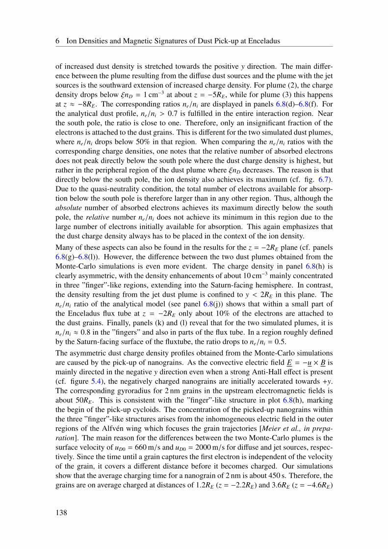
6 Ion Densities and Magnetic Signatures of Dust Pick-up at Enceladus
of increased dust density is stretched towards the positive y direction. The main differ-ence between the plume resulting from the diffuse dust sources and the plume with the jetsources is the southward extension of increased charge density. For plume (2), the chargedensity drops below ξnD = 1 cm−3 at about z = −5RE, while for plume (3) this happensat z ≈ −8RE. The corresponding ratios ne/ni are displayed in panels 6.8(d)–6.8(f). Forthe analytical dust profile, ne/ni > 0.7 is fulfilled in the entire interaction region. Nearthe south pole, the ratio is close to one. Therefore, only an insignificant fraction of theelectrons is attached to the dust grains. This is different for the two simulated dust plumes,where ne/ni drops below 50% in that region. When comparing the ne/ni ratios with thecorresponding charge densities, one notes that the relative number of absorbed electronsdoes not peak directly below the south pole where the dust charge density is highest, butrather in the peripheral region of the dust plume where ξnD decreases. The reason is thatdirectly below the south pole, the ion density also achieves its maximum (cf. fig. 6.7).Due to the quasi-neutrality condition, the total number of electrons available for absorp-tion below the south pole is therefore larger than in any other region. Thus, although theabsolute number of absorbed electrons achieves its maximum directly below the southpole, the relative number ne/ni does not achieve its minimum in this region due to thelarge number of electrons initially available for absorption. This again emphasizes thatthe dust charge density always has to be placed in the context of the ion density.Many of these aspects can also be found in the results for the z = −2RE plane (cf. panels6.8(g)–6.8(l)). However, the difference between the two dust plumes obtained from theMonte-Carlo simulations is even more evident. The charge density in panel 6.8(h) isclearly asymmetric, with the density enhancements of about 10 cm−3 mainly concentratedin three ”finger”-like regions, extending into the Saturn-facing hemisphere. In contrast,the density resulting from the jet dust plume is confined to y < 2RE in this plane. Thene/ni ratio of the analytical model (see panel 6.8(j)) shows that within a small part ofthe Enceladus flux tube at z = −2RE only about 10% of the electrons are attached tothe dust grains. Finally, panels (k) and (l) reveal that for the two simulated plumes, it isne/ni ≈ 0.8 in the ”fingers” and also in parts of the flux tube. In a region roughly definedby the Saturn-facing surface of the fluxtube, the ratio drops to ne/ni = 0.5.The asymmetric dust charge density profiles obtained from the Monte-Carlo simulationsare caused by the pick-up of nanograins. As the convective electric field E = −u × B ismainly directed in the negative y direction even when a strong Anti-Hall effect is present(cf. figure 5.4), the negatively charged nanograins are initially accelerated towards +y.The corresponding gyroradius for 2 nm grains in the upstream electromagnetic fields isabout 50RE. This is consistent with the ”finger”-like structure in plot 6.8(h), markingthe begin of the pick-up cycloids. The concentration of the picked-up nanograins withinthe three ”finger”-like structures arises from the inhomogeneous electric field in the outerregions of the Alfvén wing which focuses the grain trajectories [Meier et al., in prepa-ration]. The main reason for the differences between the two Monte-Carlo plumes is thesurface velocity of uD0 = 660 m/s and uD0 = 2000 m/s for diffuse and jet sources, respec-tively. Since the time until a grain captures the first electron is independent of the velocityof the grain, it covers a different distance before it becomes charged. Our simulationsshow that the average charging time for a nanograin of 2 nm is about 450 s. Therefore, thegrains are on average charged at distances of 1.2RE (z = −2.2RE) and 3.6RE (z = −4.6RE)
138
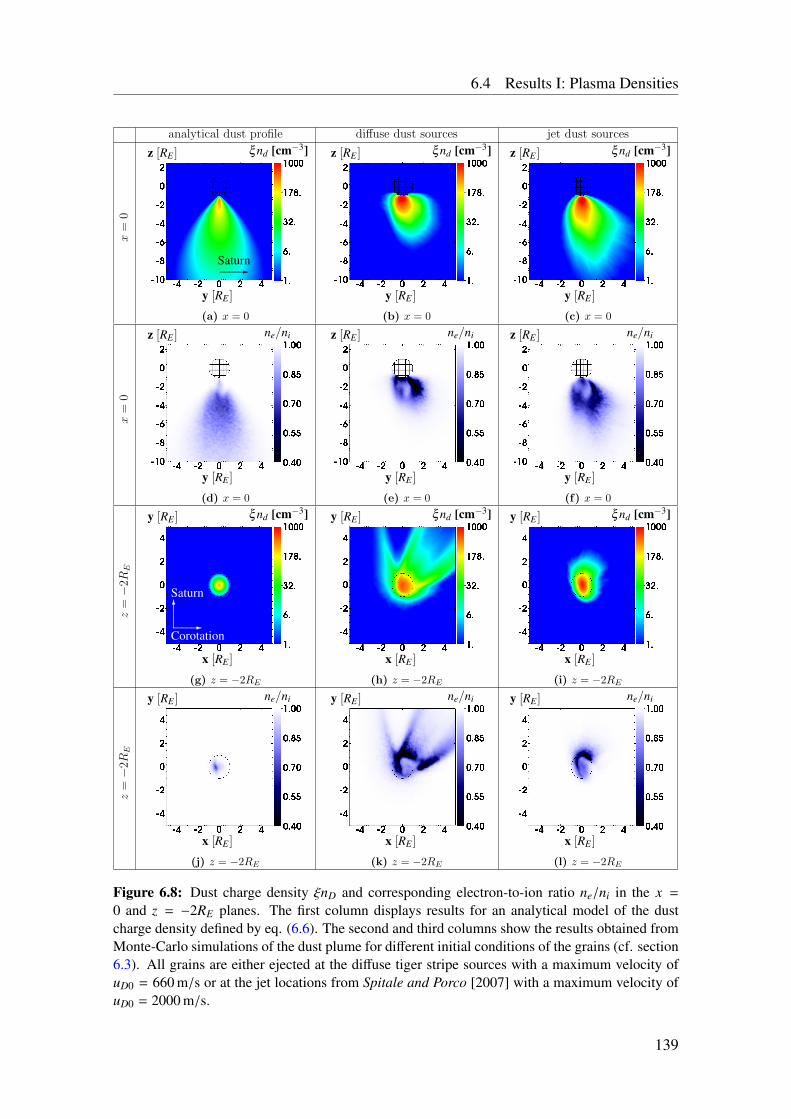
6.4 Results I: Plasma Densities
analytical dust profile diffuse dust sources jet dust sourcesx
=0
3Saturn
y [RE ]
z [RE ] ξ nd [cm−3]
1
(a) x = 0
y [RE ]
z [RE ] ξ nd [cm−3]
1
(b) x = 0
y [RE ]
z [RE ] ξ nd [cm−3]
1
(c) x = 0
x=
0
y [RE ]
z [RE ] ne/ni
1
(d) x = 0
y [RE ]
z [RE ] ne/ni
1
(e) x = 0
y [RE ]
z [RE ] ne/ni
1
(f) x = 0
z=−
2RE
3Corotation
3
Saturn
x [RE ]
y [RE ] ξ nd [cm−3]
1
(g) z = −2RE
x [RE ]
y [RE ] ξ nd [cm−3]
1
(h) z = −2RE
x [RE ]
y [RE ] ξ nd [cm−3]
1
(i) z = −2RE
z=−
2RE
x [RE ]
y [RE ] ne/ni
1
(j) z = −2RE
x [RE ]
y [RE ] ne/ni
1
(k) z = −2RE
x [RE ]
y [RE ] ne/ni
1
(l) z = −2RE
Figure 6.8: Dust charge density ξnD and corresponding electron-to-ion ratio ne/ni in the x =
0 and z = −2RE planes. The first column displays results for an analytical model of the dustcharge density defined by eq. (6.6). The second and third columns show the results obtained fromMonte-Carlo simulations of the dust plume for different initial conditions of the grains (cf. section6.3). All grains are either ejected at the diffuse tiger stripe sources with a maximum velocity ofuD0 = 660 m/s or at the jet locations from Spitale and Porco [2007] with a maximum velocity ofuD0 = 2000 m/s.
139
6 Ion Densities and Magnetic Signatures of Dust Pick-up at Enceladus
for the diffuse sources and for the jet sources, respectively. After the grains have becomecharged, they are immediately picked-up. This results in a clearly visible pick-up tail inthe z = −2RE plane for the lower grain surface velocity (see panel 6.8(h)). For the highersurface velocity, the pick-up tail is shifted to lower z values and is therefore not visible inpanel 6.8(i).Finally, we shall briefly address the question which additional effects may arise from thehigh dust charge densities in the plume. Since the dust significantly modifies the quasi-neutrality condition with respect to the situation without dust, it is qualitatively clear thatwe deal with a dusty plasma. A quantitative measure of the importance of dusty plasmaeffects is given by the ’Havnes parameter’ [Havnes et al. 1984]. This parameter cruciallydepends on the electron density and on the plasma temperatures. Since we impose alower limit on ne and assume an adiabatic law for the electrons, a reliable calculation ofthe Havnes parameter is not possible in the hybrid model. However, we are able to dis-cuss an important consequence of dusty plasma effects for the electron and ion densitiesin the plume: the overlap of the Debye spheres of the dust grains results in a potential Φc
of the dust cloud relative to the plasma potential far away from the dust cloud [Havneset al. 1984]. The effect of this potential can be illustrated with a simple example: manynanograins become negatively charged close to the south pole and subsequently thesegrains move to a region where their density is higher than the density of the surroundingions. To maintain quasi-neutrality, these grains ought to become discharged. For lowplasma densities and small grains, however, the (de)-charging time might be so large thatquasi-neutrality is violated on scales of km. Therefore, the dust cloud potential repelselectrons and attracts ions to ensure quasi-neutrality. For this reason, dusty plasma ef-fects may cause higher ion densities and may partially explain the additional ion sourcemodeled by the effective ionization frequency ν∗ (see section 6.4.2). Unfortunately, dustyplasma effects become most important for ne → 0 and thus a hybrid model is not suitableto directly model these effects.
6.5 Results II: Magnetic Field Signatures
The second part of the discussion of the simulation results focuses on the magnetic fieldin Enceladus’ vicinity. First, the impact of the three neutral plumes described in section6.2 on the magnetic field structures will be analyzed for the example of the E7 flyby. Thisflyby has already been discussed in section 5.5.3 in the previous chapter and thereforeallows to illustrate the improvements of the model.Second, we will elaborate on how the measured magnetic field can be used as a sensi-tive probe of the dust plume. A comparison between modeled and observed magneticfield signatures from the horizontal E14, E17 and E19 flybys will allow to constrain theinfluence of dust pick-up on the magnetic perturbations near Enceladus. The southwardextension of the dust plume as well as the location of the expected magnetic field decreasewith respect to the flyby trajectories will also be discussed for these flybys. Furthermore,it will be demonstrated that dust pick-up may be responsible for the magnetic field pertur-bations observed during the distant E15 flyby. By comparing MAG data from E14, E17and E18 we will also briefly address the variability of the plume.
140
6.5 Results II: Magnetic Field Signatures
Like in section 5.1, we will only show the magnetic field perturbations (∆Bx,∆By,∆Bz)throughout this section for better visualization.
6.5.1 Magnetic Field Signatures for Different Neutral Plumes (E7)
Figure 6.9 shows the simulated magnetic field perturbations together with Cassini MAGdata for the E7 flyby. MAG data are represented by black lines. The three colored linesdenote the field perturbations for the three neutral plumes #1 (red), #2 (blue), and #3(green), which have been described in section 6.2. The vertical orange lines mark thesurface of the Enceladus flux tube, i. e. the region where Cassini was located belowEnceladus. The vertical black line denotes the location of closest approach at 07:41:57UTC.When comparing the magnetic field signatures generated by the three neutral plume se-tups with the results of our previous model (cf. fig. 5.7(g)), we note some obvious differ-ences: our preceding simulations, applying an analytical neutral plume model, producedan overshoot of ∆Bx before entering and after leaving the central region of the north-ern wing where ∆Bx < 0. However, the new results based on the neutral plumes fromthe Monte-Carlo simulations generate a gradual decrease of Bx on both sides of the fluxtube in agreement with MAG data. The overshoots are no longer present. Especially thesimulation based on plume #1 shows very good agreement with the data in the inboundregion. This improvement can be attributed to the shape of the neutral plume obtainedfrom the Monte-Carlo simulations which is significantly broader compared to the verynarrow plume used by in the previous chapter (cf. figure 6.5).Surprisingly, the agreement between simulations and MAG data for the By componentwas better in the previous chapter, where observed and simulated field perturbations wereof the same strength. Our preceding simulation also reproduced the symmetric shapeof the By perturbation. Especially in the outbound segment of the E7 trajectory, the By
perturbations shown in figure 6.9 are weaker than the observed perturbations. As demon-strated in the previous chapter, however, ∆By is mainly determined by the dust plume andwill be discussed in more detail in section 6.5.3. In contrast to the previous work, the newsimulations also show both, an enhancement (∆Bz < 0) and a decrease (∆Bz > 0) in the Bz
component. However, only the region of enhanced Bz is present in MAG data. In section6.5.5, ∆Bz will be discussed in a 3D context.When comparing the results for the three neutral plumes (see figure 6.9), we find that themagnetic field perturbations generated by plumes #1 and #3 are nearly identical. Thisfinding is in agreement with the very similar large-scale density profiles of these plumesetups (cf. figure 6.2(i)). The minor differences in the fine structure of the density betweenplume #1 and plume #3 (cf. figure 6.2(j)) are not visible in the magnetic field signatures.The Bx and Bz perturbations generated by plume #2 reveal a more gradual decrease in theinbound segment of the E7 trajectory than the other plume setups. Moreover, the ”W”-likedecrease of the By component assumes its minimum value already about 0.5RE outside ofthe flux tube while the two minima of the ”W”-like By perturbations from plumes #1 and#3 are located at the surface of the flux tube. In the outbound region, the By perturbationsof all three plumes are nearly identical. These differences are probably caused by thelarger neutral density of plume #2 in the inbound region of E7 (cf. plots 6.2(i) and 6.2(j)).
141
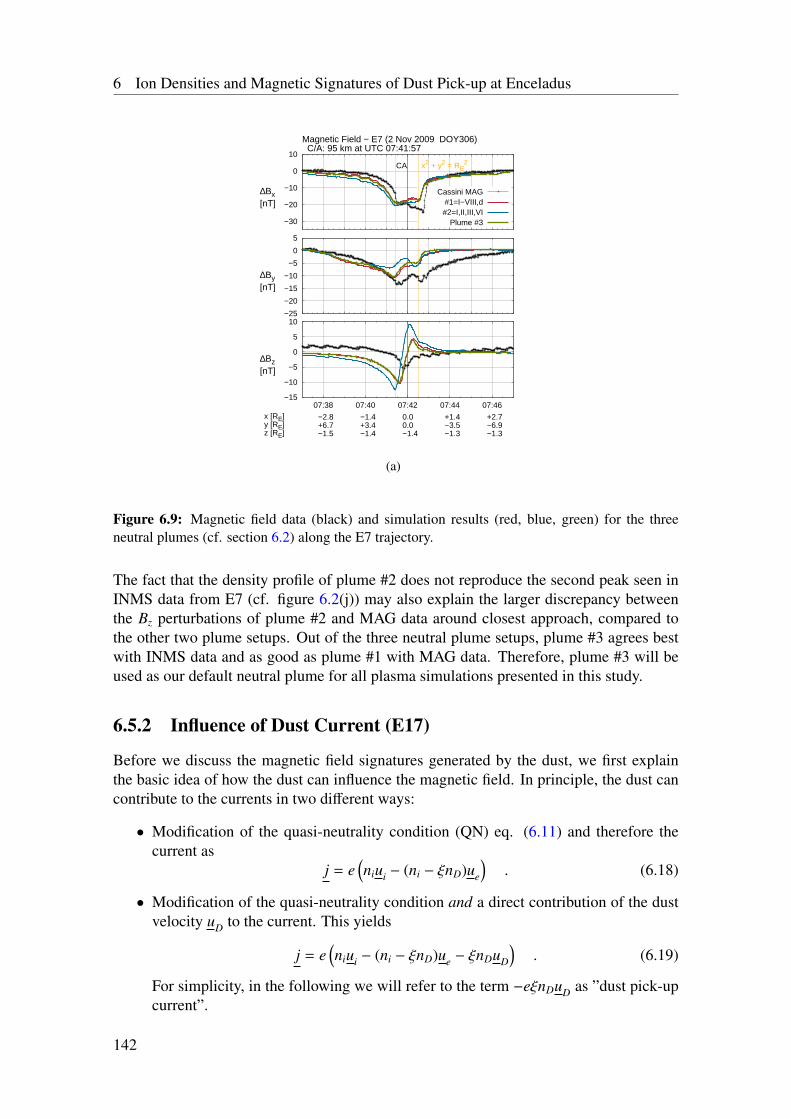
6 Ion Densities and Magnetic Signatures of Dust Pick-up at Enceladus
−30
−20
−10
0
10
07:37 07:38 07:39 07:40 07:41 07:42 07:43 07:44 07:45 07:46 07:47
Magnetic Field − E7 (2 Nov 2009 DOY306) C/A: 95 km at UTC 07:41:57
x2 + y2 = RE2CA
∆Bx [nT]
Cassini MAG#1=I−VIII,d#2=I,II,III,VI
Plume #3
−25
−20
−15
−10
−5
0
5
07:37 07:38 07:39 07:40 07:41 07:42 07:43 07:44 07:45 07:46 07:47
∆By [nT]
−15
−10
−5
0
5
10
07:38 07:40 07:42 07:44 07:46x [RE]y [RE]z [RE]
−2.8+6.7−1.5
−1.4+3.4−1.4
0.00.0−1.4
+1.4−3.5−1.3
+2.7−6.9−1.3
∆Bz [nT]
(a)
Figure 6.9: Magnetic field data (black) and simulation results (red, blue, green) for the threeneutral plumes (cf. section 6.2) along the E7 trajectory.
The fact that the density profile of plume #2 does not reproduce the second peak seen inINMS data from E7 (cf. figure 6.2(j)) may also explain the larger discrepancy betweenthe Bz perturbations of plume #2 and MAG data around closest approach, compared tothe other two plume setups. Out of the three neutral plume setups, plume #3 agrees bestwith INMS data and as good as plume #1 with MAG data. Therefore, plume #3 will beused as our default neutral plume for all plasma simulations presented in this study.
6.5.2 Influence of Dust Current (E17)
Before we discuss the magnetic field signatures generated by the dust, we first explainthe basic idea of how the dust can influence the magnetic field. In principle, the dust cancontribute to the currents in two different ways:
• Modification of the quasi-neutrality condition (QN) eq. (6.11) and therefore thecurrent as
j = e(niui − (ni − ξnD)ue
). (6.18)
• Modification of the quasi-neutrality condition and a direct contribution of the dustvelocity uD to the current. This yields
j = e(niui − (ni − ξnD)ue − ξnDuD
). (6.19)
For simplicity, in the following we will refer to the term −eξnDuD as ”dust pick-upcurrent”.
142
6.5 Results II: Magnetic Field Signatures
The first case has already been analyzed in the previous chapter. However, the resultsfor the dust plume (see section 6.4.3) have shown that a significant amount of the dustgrains is being charged and picked up. These grains possess a non-negligible velocityperpendicular to the magnetic field and we need to investigate if this velocity makes anoticeable contribution to the currents and magnetic field perturbations.For this reason, figure 6.10(a) shows a comparison between Cassini observations (black)and the results of two simulation runs for the E17 flyby. These simulations are character-ized by: (1, red) the hybrid simulation uses only the dust density profile ξnD(x) obtainedfrom the Monte-Carlo simulations. The corresponding dust velocity uD is set to zero in thehybrid simulation. (2, blue) the identical dust profile ξnD(x) is applied, but the dust pick-up current is also included. This is our default setup. Again, the vertical orange and blacklines indicate the surface of the Enceladus flux tube and closest approach, respectively.Since the magnetic field observations from the E17 flyby have not yet been presented inthe literature, we discuss them in some more detail here. The shape of the ∆Bx signatureis very similar to the ”U”-shape of ∆Bx from E7 and corresponds to Cassini’s passagethrough the center of the northern Alfvén wing. However, the Bx decrease observed duringE17 possesses a depth of about 30 nT, i. e. the perturbation is about a factor of 1.5 strongerthan during E7 (∆Bx = −20 nT). This finding is consistent with a positive correlationbetween upstream density n0 and the Bx perturbation (in the far field Alfvén wing solution,it is ∆Bx ∼
√n0), since the upstream density was n0 = 110 cm−3 for E17 and only n0 =
60 cm−3 during E7 (cf. table 2.2). Inbound, Bx decreases gradually from ∆Bx = 0 to∆Bx = −30 nT. Outbound, however, ∆Bx increases by more than 10 nT within 10 kmaround 18:30:44 UTC across the surface of the Enceladus flux tube. This discontinuity-like jump probably results from the hemisphere coupling current system predicted by Sauret al. [2007]. Furthermore, this behavior is consistent with MAG data from E7 and E9which also exhibit such a discontinuity-like jump across the (y > 0) surface of the fluxtube, but not across the (y < 0) surface [Simon et al. 2011b]. The By perturbation exhibitsan even more asymmetric shape. Inbound, ∆By decreases by about 10 nT from 18:29:00to 18:29:30 UTC. This decrease is followed by a very sharp dip reaching ∆By = −20 nTnear closest approach. After closest approach ∆By increases to ∆By = −10 nT. Acrossthe (y > 0) surface of the flux tube, one can again see a discontinuity-like decrease of theBy component by 5 nT. Outbound, ∆By gradually increases until the perturbation vanishesat y ≥ 10RE. The observed Bz perturbation possesses a ”W”-like shape with a peakmagnitude of about ∆Bz = −12 nT. The local maximum in the middle of the ”W” of∆Bz = −5 nT was observed at closest approach. This Bz perturbation is consistent withthe pile-up of the magnetic field at the ramside of the plume, as will be discussed insection 6.5.5.The two simulations shown in figure 6.10(a) reproduce the key features of the data. Theinbound decrease of Bx is perfectly matched by our model. Outbound, however, the sim-ulations do not show the sharp Bx increase seen in the data and increase more gradual tothe background value in the (x > 1RE, y > 1RE) sector. The peak strength of the simulatedBx perturbations is about 5 nT too weak in both cases. For the By component, the simu-lations show a similar inbound-outbound asymmetry as the observation. In the outboundsegment, the By perturbations are few nT stronger than in the observation. Within the fluxtube, however, our simulations do not reproduce the dip in ∆By. In panel 6.10(b), we dis-
143
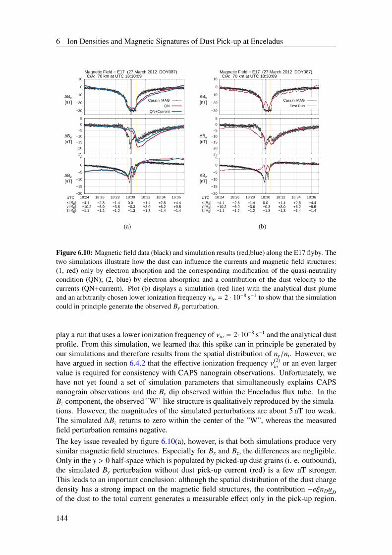
6 Ion Densities and Magnetic Signatures of Dust Pick-up at Enceladus
−30
−20
−10
0
10
18:24 18:26 18:28 18:30 18:32 18:34 18:36
Magnetic Field − E17 (27 March 2012 DOY087) C/A: 70 km at UTC 18:30:09
∆Bx [nT] Cassini MAG
QN
QN+Current
−25
−20
−15
−10
−5
0
5
18:24 18:26 18:28 18:30 18:32 18:34 18:36
∆By [nT]
−20
−15
−10
−5
0
5
18:24 18:26 18:28 18:30 18:32 18:34 18:36UTCx [RE]y [RE]z [RE]
−4.1−10.2−1.1
−2.8−6.9−1.2
−1.4−3.6−1.2
0.0−0.3−1.3
+1.4+3.0−1.3
+2.8+6.2−1.4
+4.4+9.5−1.4
∆Bz [nT]
(a)
−30
−20
−10
0
10
18:24 18:26 18:28 18:30 18:32 18:34 18:36
Magnetic Field − E17 (27 March 2012 DOY087) C/A: 70 km at UTC 18:30:09
∆Bx [nT] Cassini MAG
Test Run
−25
−20
−15
−10
−5
0
5
18:24 18:26 18:28 18:30 18:32 18:34 18:36
∆By [nT]
−20
−15
−10
−5
0
5
18:24 18:26 18:28 18:30 18:32 18:34 18:36UTCx [RE]y [RE]z [RE]
−4.1−10.2−1.1
−2.8−6.9−1.2
−1.4−3.6−1.2
0.0−0.3−1.3
+1.4+3.0−1.3
+2.8+6.2−1.4
+4.4+9.5−1.4
∆Bz [nT]
(b)
Figure 6.10: Magnetic field data (black) and simulation results (red,blue) along the E17 flyby. Thetwo simulations illustrate how the dust can influence the currents and magnetic field structures:(1, red) only by electron absorption and the corresponding modification of the quasi-neutralitycondition (QN); (2, blue) by electron absorption and a contribution of the dust velocity to thecurrents (QN+current). Plot (b) displays a simulation (red line) with the analytical dust plumeand an arbitrarily chosen lower ionization frequency νio = 2 · 10−8 s−1 to show that the simulationcould in principle generate the observed By perturbation.
play a run that uses a lower ionization frequency of νio = 2·10−8 s−1 and the analytical dustprofile. From this simulation, we learned that this spike can in principle be generated byour simulations and therefore results from the spatial distribution of ne/ni. However, wehave argued in section 6.4.2 that the effective ionization frequency ν(2)
io or an even largervalue is required for consistency with CAPS nanograin observations. Unfortunately, wehave not yet found a set of simulation parameters that simultaneously explains CAPSnanograin observations and the By dip observed within the Enceladus flux tube. In theBz component, the observed ”W”-like structure is qualitatively reproduced by the simula-tions. However, the magnitudes of the simulated perturbations are about 5 nT too weak.The simulated ∆Bz returns to zero within the center of the ”W”, whereas the measuredfield perturbation remains negative.The key issue revealed by figure 6.10(a), however, is that both simulations produce verysimilar magnetic field structures. Especially for Bx and Bz, the differences are negligible.Only in the y > 0 half-space which is populated by picked-up dust grains (i. e. outbound),the simulated By perturbation without dust pick-up current (red) is a few nT stronger.This leads to an important conclusion: although the spatial distribution of the dust chargedensity has a strong impact on the magnetic field structures, the contribution −eξnDuDof the dust to the total current generates a measurable effect only in the pick-up region.
144
6.5 Results II: Magnetic Field Signatures
There, the dust velocity is large enough to have a small influence on the strength of the By
perturbation. The overall shape of the By perturbations, however, remains completely un-affected by the inclusion of the non-vanishing dust velocity. This finding can be explainedwith the analytical description of the currents associated with dust according to equation(5.12). For convenience, the expression for the current jx is repeated here,
jx = −eniui
(ν2
i
ν2i + Ω2
i
−ξnD
ni
(1 −
uD,x
ui
)). (6.20)
The negative By perturbation measured along E17 implies a positive jx (cf. section 5.2).From equation (6.20), it is then clear that the second term in brackets has to be larger thanthe first one (Anti-Hall effect). If the x component of the dust velocity uD,x is significantlysmaller than the ion bulk velocity, the major effect of the dust on jx arises from the dustcharge density ξnD. South of Enceladus, |uD,x| ui is well fulfilled. In that region, onlythe spatial distribution of the dust charge density ξnD(x) has a non-negligible impact onthe magnetic field structures. Outside the flux tube at y > 1RE, the part of the ”finger”-likestructure in ξnD intersected by E17 is tilted towards positive x (cf. figure 6.8(h)). Thisimplies a non-vanishing uD,x > 0 due to dust pick-up. The second term in eq. (6.20) istherefore reduced (but is still larger than the first term, since the Anti-Hall effect is stillpresent) and leads to a weaker By perturbation in the simulation including the dust pick-upcurrent (cf. figure 6.10(a)).The Bx perturbation is mainly generated by the current in y direction which can be ex-pressed as (cf. eq. (5.14))
jy = −eniui
(νiΩi
ν2i + Ω2
i
+ξnD
ni
uD,y
ui
). (6.21)
A positive uD,y component of the nanograins therefore leads to a stronger current in agree-ment with the slightly stronger ∆Bx in the simulation including uD (see figure 6.10).To sum up, only in the (x > 0, y > 0) sector the dust velocity due to pick-up has a no-ticeable influence on the magnetic field structures. Anywhere else, only the modificationof the quasi-neutrality condition due to the absorption of electrons by the dust grains isimportant for the magnetic field perturbations.
6.5.3 Pick-up and Length of Dust Plume (E14 and E19)
To analyze how the spatial distribution of the dust charge density ξnD affects the magneticfield structures, we apply the three dust distributions described in section 6.4.3. Figure6.11 displays 2D plots of the Bx and By components from our simulations as well as MAGdata and results for E14 and E19. The first column (panels (a),(d),(g)) shows the resultsfor the analytical dust plume from eq. (6.6). The middle column displays the results forthe dust plume from the Monte-Carlo simulations with the diffuse sources only and thethird column shows the results for the dust plume using only the jet sources. Panels (a)–(f)display ∆Bx and ∆By at z = −1.5RE, i. e. approximately in the plane where the E7, E14,E17 and E19 flybys took place. The projections of the flyby trajectories on this planeare also plotted. ∆By is also provided in the y = 0 plane in panels (g)–(i) along with the
145
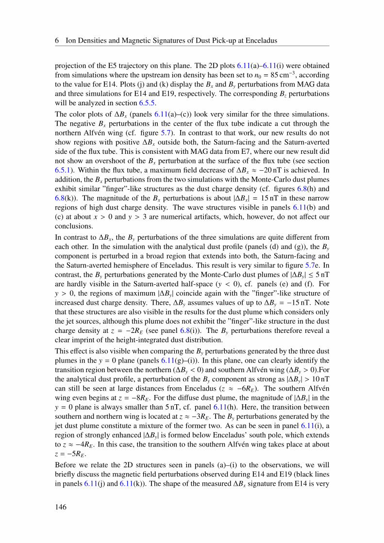
6 Ion Densities and Magnetic Signatures of Dust Pick-up at Enceladus
projection of the E5 trajectory on this plane. The 2D plots 6.11(a)–6.11(i) were obtainedfrom simulations where the upstream ion density has been set to n0 = 85 cm−3, accordingto the value for E14. Plots (j) and (k) display the Bx and By perturbations from MAG dataand three simulations for E14 and E19, respectively. The corresponding Bz perturbationswill be analyzed in section 6.5.5.The color plots of ∆Bx (panels 6.11(a)–(c)) look very similar for the three simulations.The negative Bx perturbations in the center of the flux tube indicate a cut through thenorthern Alfvén wing (cf. figure 5.7). In contrast to that work, our new results do notshow regions with positive ∆Bx outside both, the Saturn-facing and the Saturn-avertedside of the flux tube. This is consistent with MAG data from E7, where our new result didnot show an overshoot of the Bx perturbation at the surface of the flux tube (see section6.5.1). Within the flux tube, a maximum field decrease of ∆Bx ≈ −20 nT is achieved. Inaddition, the Bx perturbations from the two simulations with the Monte-Carlo dust plumesexhibit similar ”finger”-like structures as the dust charge density (cf. figures 6.8(h) and6.8(k)). The magnitude of the Bx perturbations is about |∆Bx| = 15 nT in these narrowregions of high dust charge density. The wave structures visible in panels 6.11(b) and(c) at about x > 0 and y > 3 are numerical artifacts, which, however, do not affect ourconclusions.In contrast to ∆Bx, the By perturbations of the three simulations are quite different fromeach other. In the simulation with the analytical dust profile (panels (d) and (g)), the By
component is perturbed in a broad region that extends into both, the Saturn-facing andthe Saturn-averted hemisphere of Enceladus. This result is very similar to figure 5.7e. Incontrast, the By perturbations generated by the Monte-Carlo dust plumes of |∆By| ≤ 5 nTare hardly visible in the Saturn-averted half-space (y < 0), cf. panels (e) and (f). Fory > 0, the regions of maximum |∆By| coincide again with the ”finger”-like structure ofincreased dust charge density. There, ∆By assumes values of up to ∆By = −15 nT. Notethat these structures are also visible in the results for the dust plume which considers onlythe jet sources, although this plume does not exhibit the ”finger”-like structure in the dustcharge density at z = −2RE (see panel 6.8(i)). The By perturbations therefore reveal aclear imprint of the height-integrated dust distribution.This effect is also visible when comparing the By perturbations generated by the three dustplumes in the y = 0 plane (panels 6.11(g)–(i)). In this plane, one can clearly identify thetransition region between the northern (∆By < 0) and southern Alfvén wing (∆By > 0).Forthe analytical dust profile, a perturbation of the By component as strong as |∆By| > 10 nTcan still be seen at large distances from Enceladus (z ≈ −6RE). The southern Alfvénwing even begins at z = −8RE. For the diffuse dust plume, the magnitude of |∆By| in they = 0 plane is always smaller than 5 nT, cf. panel 6.11(h). Here, the transition betweensouthern and northern wing is located at z ≈ −3RE. The By perturbations generated by thejet dust plume constitute a mixture of the former two. As can be seen in panel 6.11(i), aregion of strongly enhanced |∆By| is formed below Enceladus’ south pole, which extendsto z ≈ −4RE. In this case, the transition to the southern Alfvén wing takes place at aboutz = −5RE.Before we relate the 2D structures seen in panels (a)–(i) to the observations, we willbriefly discuss the magnetic field perturbations observed during E14 and E19 (black linesin panels 6.11(j) and 6.11(k)). The shape of the measured ∆Bx signature from E14 is very
146
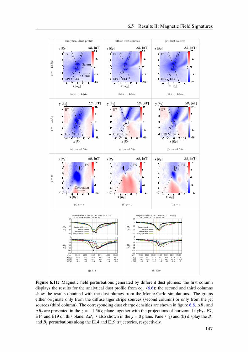
6.5 Results II: Magnetic Field Signatures
analytical dust profile diffuse dust sources jet dust sources
z=−
1.5R
E
E19 E14
AAU
E7
3Corot.
3
Saturn
x [RE ]
y [RE ] ∆Bx [nT]
1(a) z = −1.5RE
E19 E14
AAU
E7
x [RE ]
y [RE ] ∆Bx [nT]
1(b) z = −1.5RE
E19 E14
AAU
E7
x [RE ]
y [RE ] ∆Bx [nT]
1(c) z = −1.5RE
z=−
1.5R
E
E19 E14
AAU
E7
x [RE ]
y [RE ] ∆By [nT]
1(d) z = −1.5RE
E19 E14
AAU
E7
x [RE ]
y [RE ] ∆By [nT]
1(e) z = −1.5RE
E19 E14
AAU
E7
x [RE ]
y [RE ] ∆By [nT]
1(f) z = −1.5RE
y=
0
E5
3Corotation
x [RE ]
z [RE ] ∆By [nT]
1(g) y = 0
E5
x [RE ]
z [RE ] ∆By [nT]
1(h) y = 0
E5
x [RE ]
z [RE ] ∆By [nT]
1(i) y = 0
−30
−20
−10
0
10
13:48 13:50 13:52 13:54 13:56 13:58
Magnetic Field − E14 (01 Oct 2011 DOY274) C/A: 95 km at UTC 13:52:26
∆Bx [nT]
Cassini MAGjet dust
diffuse dustanalytical dust
−25
−20
−15
−10
−5
0
5
13:48 13:50 13:52 13:54 13:56 13:58UTCx [RE]y [RE]z [RE]
−3.0−7.2−1.3
−1.7−4.0−1.3
−0.3−0.7−1.4
+1.1+2.5−1.4
+2.6+5.7−1.4
+4.1+8.9−1.4
∆By [nT]
(j) E14
−30
−20
−10
0
10
09:26 09:28 09:30 09:32 09:34 09:36 09:38
Magnetic Field − E19 (2 May 2012 DOY123) C/A: 70 km at UTC 09:31:29
∆Bx [nT]
Cassini MAGjet dust
diffuse dustanalytical dust
−25
−20
−15
−10
−5
0
5
09:26 09:28 09:30 09:32 09:34 09:36 09:38UTCx [RE]y [RE]z [RE]
−4.1−9.0−1.1
−2.7−5.6−1.1
−1.4−2.3−1.2
0.0+1.0−1.2
+1.4+4.3−1.3
+2.9+7.6−1.3
+4.4+10.8−1.3
∆By [nT]
(k) E19
Figure 6.11: Magnetic field perturbations generated by different dust plumes: the first columndisplays the results for the analytical dust profile from eq. (6.6); the second and third columnsshow the results obtained with the dust plumes from the Monte-Carlo simulations. The grainseither originate only from the diffuse tiger stripe sources (second column) or only from the jetsources (third column). The corresponding dust charge densities are shown in figure 6.8. ∆Bx and∆By are presented in the z = −1.5RE plane together with the projections of horizontal flybys E7,E14 and E19 on this plane. ∆By is also shown in the y = 0 plane. Panels (j) and (k) display the Bx
and By perturbations along the E14 and E19 trajectories, respectively.147
6 Ion Densities and Magnetic Signatures of Dust Pick-up at Enceladus
similar to E7 and E17. However, the peak magnitude of the perturbation seen during E14(∆Bx = −25 nT) is about 5 nT smaller than for E17. This difference might partially arisefrom the different upstream densities of n0 = 85 cm−3 for E14, compared to n0 = 110 cm−3
for E17 (cf. table 2.2). In the center of the flux tube, the Alfvén wing far field solutionfulfills ∆Bx ∼
√n0. This estimation is roughly consistent with the observed perturbations:
∆Bx(E14)/∆Bx(E17) = 0.8 ≈√
n0(E14)/√
n0(E17) = 0.9. Inbound of E19, the observeddecrease to the maximum perturbation of about ∆Bx = −20 nT occurs rather gradualcompared to the ”U”-shape seen during the other flybys (fig. 6.11(k)). In addition, the Bx
perturbation observed during E19 does not show the small local maximum around closestapproach which was seen during E7, E14 and E17. The reason is the slight upstreamdisplacement of the E19 trajectory compared to E14 and E17. In the outbound regionsof E14 and E19, the magnetometer detected a discontinuity-like jump of more than 5nT when crossing the surface of the Enceladus flux tube. In both cases, this structurepossesses a thickness of less than 10 km. The By perturbation observed during E14 looksquite similar to the signature seen during E17 (see figure 6.10), but is about 5 nT stronger.However, the sharp dip of ∆By = −20 nT before closest approach has the same magnitudeas seen during E17. This is different for E19, where the measured By is |∆By| < 10 nT.The colored lines which are also plotted in panels 6.11(j) and 6.11(k) are the magneticfield signatures from the three simulations with the different dust plumes. For ∆Bx, allthree simulations produce a very similar signature. The strength of the simulated per-turbations of ∆Bx ≈ −20 nT is weaker than the perturbation of ∆Bx ≈ −25 nT observedduring E14. The magnitude of the dip seen during E19 is well reproduced. The simula-tions succeed in reproducing both, the location and the steepness of the inbound decreasein Bx. The simulated ∆Bx also shows the small local maximum around closest approachof E14. The location of the ∆Bx minimum seen during E14 and E19 at the outbound edgeof the flux tube is reproduced as well. Outside the flux tube at y > 0, the discrepanciesbetween data and simulations are larger for both flybys: the simulated fields gradually in-crease to the background value while the data reveal a discontinuity-like enhancement ofBx across the flux tube. Again, the observed structure is probably caused by hemispherecoupling currents [Saur et al. 2007].The By component exhibits stronger differences between the three simulations. For E14(panel 6.11(j)), the inbound perturbation caused by the analytical dust plume (green) al-ready commences at about 13:49 UTC, whereas the measured field is still unperturbeduntil 13:51 UTC. In the outbound region, the magnitude of the By perturbations is slightlyunderestimated by the analytical dust plume. Within the Enceladus flux tube, however,the analytical dust plume yields a better fit to the data than the simulated dust plumes.Unlike the analytical profile, both Monte-Carlo dust plumes succeed in reproducing theBy perturbation in the outbound region of E14. Below the south pole, however, the dif-fuse dust plume (blue) does not produce a noticeable ∆By, while the jet dust plume (red)generates a By perturbation with a strength of about 50% of the measured ∆By, i. e. thisis still weaker than the perturbations generated by the analytical dust profile.These results lead to number of important conclusions, especially when one considersthe underlying dust densities (fig. 6.8). The asymmetry of the By perturbations inboundand outbound of E14, E17 and E19 is reproduced only by the simulated dust plumes.Therefore, these asymmetries are associated with the deformation of the plume due to
148
6.5 Results II: Magnetic Field Signatures
dust pick-up. It is, however, surprising that even for the analytical dust plume – i. e.without pick-up – we find that By is also perturbed in the (y > 1RE) sector (see panel6.11(d)). Since for the analytical plume, this perturbation can also be seen at (y < −1RE),we conclude that dust pick-up is not only responsible for generating the By perturbationsin the Saturn-facing hemisphere (y > 1RE), but the pick-up process also leads to the ab-sence of By perturbations in the Saturn-averted hemisphere. Due to pick-up, this sector isessentially devoid of charged grains which results in a weaker or vanishing By perturba-tion. Thus, the asymmetry of the observed By perturbations is a direct consequence of thepick-up of negatively charged dust grains.The results for the southward extension and strength of the By perturbations seem to beeven more surprising. Compared to the Monte-Carlo plume models, the dust charge den-sity directly below the south pole is much smaller for the analytical model (cf. figure6.8). Nevertheless, the analytical plume model generates much stronger and more ex-tended negative By perturbations south of Enceladus than the other two plumes (cf. plots6.11(g)–(i)). In particular, the high dust charge density and strong electron absorption ofthe diffuse dust plume does not produce a noticeable negative By directly below the southpole. The dust charge densities of the three dust plumes (see figure 6.8) suggest that nei-ther the absolute value of the charge density ξnD nor the relative amount of free electronsdirectly below Enceladus determines the location of the draping center (i.e., the locationof the transition between northern and southern Alfvén wing, cf. panels 6.11(g)–(i)), butthe southward extension of the region where a considerable fraction of the electrons isattached to the dust (see panels 6.8(d)–(f)).Furthermore, MAG data from E14 and E17 reveal a strong ∆By directly below the southpole (see plots 6.10 and 6.11(j)). Therefore, even the observed magnetic field perturba-tions from these horizontal flybys require a sufficiently large southward extension of thedust plume. In addition, MAG data from the steep encounters E3 – E6 exhibit a nega-tive By perturbation even at z ≈ −4RE (see previous chapter). In combination with theresults presented in panels 6.11(h) and 6.11(i), these observations imply that the south-ward extension of the dust plume is larger than seen in the results with the Monte-Carlodust plume that uses only the diffuse sources. Hence, Enceladus’ dust plume is probablybetter described by the model that comprises only the jet sources. Most of the nanograinsmight therefore be ejected with velocities as high as uD0 = 2000 m/s, implying a Machnumber of M = 6 for the neutral gas. This finding is roughly consistent with the model ofPostberg et al. [2011], who concluded that small, non-salty grains are ejected in the fastjets with uD0 = 1200 m/s while the larger grains are ejected from the tiger stripe sourcesat lower velocities. However, it is possible that – apart from the high surface velocity– other effects like changes in the value of ionization rate in combination with a differ-ent dust production rate lead to lower numbers of ”free” electrons and in consequence,a sufficiently long charging time of the grains. This would result in a further southwardextension of the charged dust plume and could therefore also explain the magnetic fieldobservations. Furthermore, additional or stronger jets pointing towards upstream and inthe anti-Saturnward direction could in principle produce a stronger By perturbation belowthe south pole as well.
149
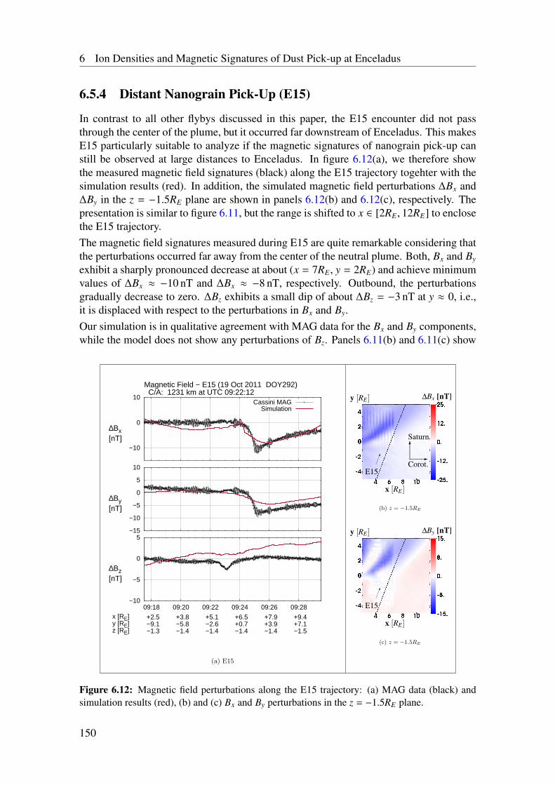
6 Ion Densities and Magnetic Signatures of Dust Pick-up at Enceladus
6.5.4 Distant Nanograin Pick-Up (E15)
In contrast to all other flybys discussed in this paper, the E15 encounter did not passthrough the center of the plume, but it occurred far downstream of Enceladus. This makesE15 particularly suitable to analyze if the magnetic signatures of nanograin pick-up canstill be observed at large distances to Enceladus. In figure 6.12(a), we therefore showthe measured magnetic field signatures (black) along the E15 trajectory togehter with thesimulation results (red). In addition, the simulated magnetic field perturbations ∆Bx and∆By in the z = −1.5RE plane are shown in panels 6.12(b) and 6.12(c), respectively. Thepresentation is similar to figure 6.11, but the range is shifted to x ∈ [2RE, 12RE] to enclosethe E15 trajectory.The magnetic field signatures measured during E15 are quite remarkable considering thatthe perturbations occurred far away from the center of the neutral plume. Both, Bx and By
exhibit a sharply pronounced decrease at about (x = 7RE, y = 2RE) and achieve minimumvalues of ∆Bx ≈ −10 nT and ∆Bx ≈ −8 nT, respectively. Outbound, the perturbationsgradually decrease to zero. ∆Bz exhibits a small dip of about ∆Bz = −3 nT at y ≈ 0, i.e.,it is displaced with respect to the perturbations in Bx and By.Our simulation is in qualitative agreement with MAG data for the Bx and By components,while the model does not show any perturbations of Bz. Panels 6.11(b) and 6.11(c) show
−10
0
10
09:18 09:20 09:22 09:24 09:26 09:28
Magnetic Field − E15 (19 Oct 2011 DOY292) C/A: 1231 km at UTC 09:22:12
∆Bx [nT]
Cassini MAGSimulation
−15
−10
−5
0
5
10
09:18 09:20 09:22 09:24 09:26 09:28
∆By [nT]
−10
−5
0
5
09:18 09:20 09:22 09:24 09:26 09:28x [RE]y [RE]z [RE]
+2.5−9.1−1.3
+3.8−5.8−1.4
+5.1−2.6−1.4
+6.5+0.7−1.4
+7.9+3.9−1.4
+9.4+7.1−1.5
∆Bz [nT]
(a) E15
E15
3Corot.
3
Saturn
x [RE ]
y [RE ] ∆Bx [nT]
1(b) z = −1.5RE
E15
x [RE ]
y [RE ] ∆By [nT]
1(c) z = −1.5RE
Figure 6.12: Magnetic field perturbations along the E15 trajectory: (a) MAG data (black) andsimulation results (red), (b) and (c) Bx and By perturbations in the z = −1.5RE plane.
150
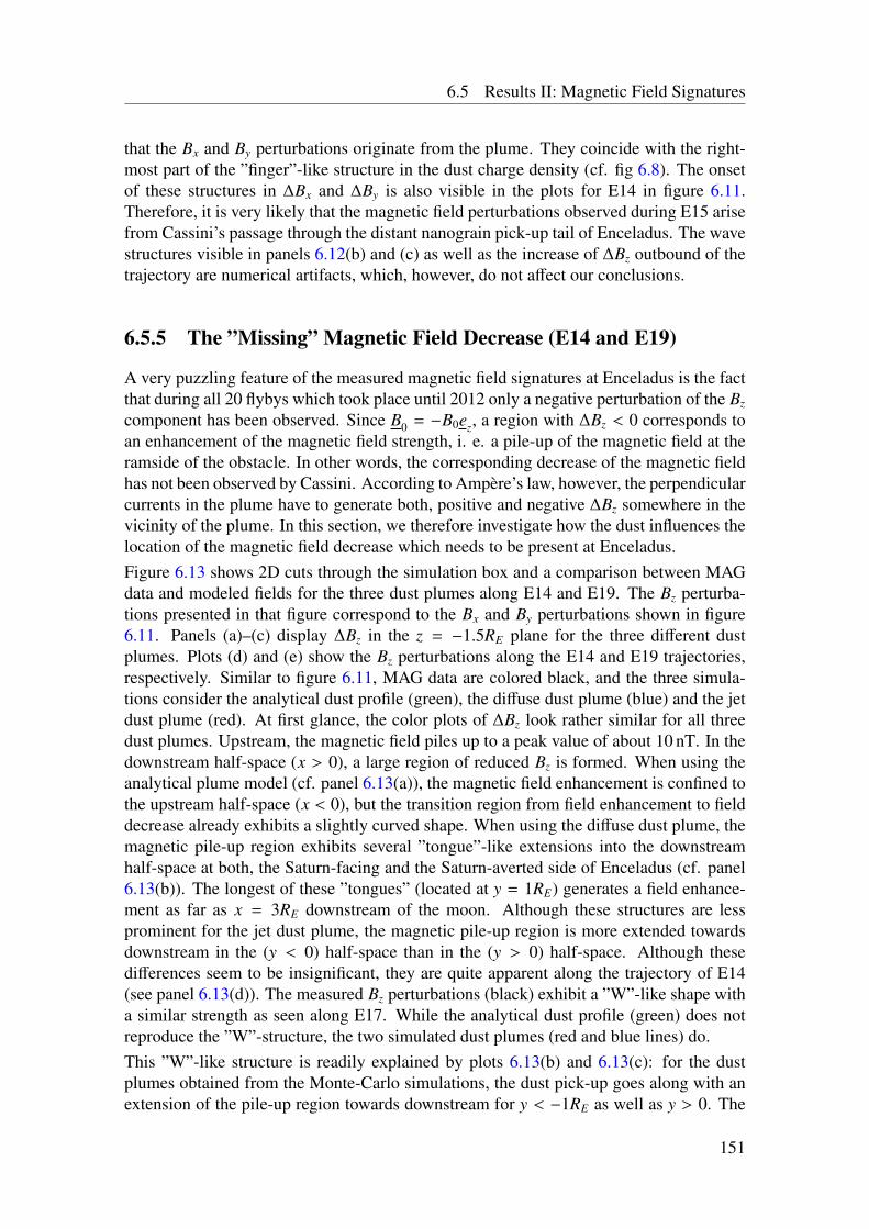
6.5 Results II: Magnetic Field Signatures
that the Bx and By perturbations originate from the plume. They coincide with the right-most part of the ”finger”-like structure in the dust charge density (cf. fig 6.8). The onsetof these structures in ∆Bx and ∆By is also visible in the plots for E14 in figure 6.11.Therefore, it is very likely that the magnetic field perturbations observed during E15 arisefrom Cassini’s passage through the distant nanograin pick-up tail of Enceladus. The wavestructures visible in panels 6.12(b) and (c) as well as the increase of ∆Bz outbound of thetrajectory are numerical artifacts, which, however, do not affect our conclusions.
6.5.5 The ”Missing” Magnetic Field Decrease (E14 and E19)
A very puzzling feature of the measured magnetic field signatures at Enceladus is the factthat during all 20 flybys which took place until 2012 only a negative perturbation of the Bz
component has been observed. Since B0 = −B0ez, a region with ∆Bz < 0 corresponds toan enhancement of the magnetic field strength, i. e. a pile-up of the magnetic field at theramside of the obstacle. In other words, the corresponding decrease of the magnetic fieldhas not been observed by Cassini. According to Ampère’s law, however, the perpendicularcurrents in the plume have to generate both, positive and negative ∆Bz somewhere in thevicinity of the plume. In this section, we therefore investigate how the dust influences thelocation of the magnetic field decrease which needs to be present at Enceladus.Figure 6.13 shows 2D cuts through the simulation box and a comparison between MAGdata and modeled fields for the three dust plumes along E14 and E19. The Bz perturba-tions presented in that figure correspond to the Bx and By perturbations shown in figure6.11. Panels (a)–(c) display ∆Bz in the z = −1.5RE plane for the three different dustplumes. Plots (d) and (e) show the Bz perturbations along the E14 and E19 trajectories,respectively. Similar to figure 6.11, MAG data are colored black, and the three simula-tions consider the analytical dust profile (green), the diffuse dust plume (blue) and the jetdust plume (red). At first glance, the color plots of ∆Bz look rather similar for all threedust plumes. Upstream, the magnetic field piles up to a peak value of about 10 nT. In thedownstream half-space (x > 0), a large region of reduced Bz is formed. When using theanalytical plume model (cf. panel 6.13(a)), the magnetic field enhancement is confined tothe upstream half-space (x < 0), but the transition region from field enhancement to fielddecrease already exhibits a slightly curved shape. When using the diffuse dust plume, themagnetic pile-up region exhibits several ”tongue”-like extensions into the downstreamhalf-space at both, the Saturn-facing and the Saturn-averted side of Enceladus (cf. panel6.13(b)). The longest of these ”tongues” (located at y = 1RE) generates a field enhance-ment as far as x = 3RE downstream of the moon. Although these structures are lessprominent for the jet dust plume, the magnetic pile-up region is more extended towardsdownstream in the (y < 0) half-space than in the (y > 0) half-space. Although thesedifferences seem to be insignificant, they are quite apparent along the trajectory of E14(see panel 6.13(d)). The measured Bz perturbations (black) exhibit a ”W”-like shape witha similar strength as seen along E17. While the analytical dust profile (green) does notreproduce the ”W”-structure, the two simulated dust plumes (red and blue lines) do.This ”W”-like structure is readily explained by plots 6.13(b) and 6.13(c): for the dustplumes obtained from the Monte-Carlo simulations, the dust pick-up goes along with anextension of the pile-up region towards downstream for y < −1RE as well as y > 0. The
151
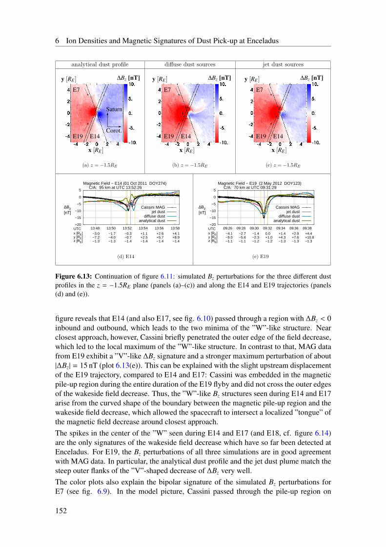
6 Ion Densities and Magnetic Signatures of Dust Pick-up at Enceladus
analytical dust profile diffuse dust sources jet dust sources
E19 E14
AAU
E7
3Corot.
3
Saturn
x [RE ]
y [RE ] ∆Bz [nT]
1(a) z = −1.5RE
E19 E14
AAU
E7
x [RE ]
y [RE ] ∆Bz [nT]
1(b) z = −1.5RE
E19 E14
AAU
E7
x [RE ]
y [RE ] ∆Bz [nT]
1(c) z = −1.5RE
−20
−15
−10
−5
0
5
13:48 13:50 13:52 13:54 13:56 13:58
Magnetic Field − E14 (01 Oct 2011 DOY274) C/A: 95 km at UTC 13:52:26
UTCx [RE]y [RE]z [RE]
−3.0−7.2−1.3
−1.7−4.0−1.3
−0.3−0.7−1.4
+1.1+2.5−1.4
+2.6+5.7−1.4
+4.1+8.9−1.4
∆Bz [nT]
Cassini MAGjet dust
diffuse dustanalytical dust
(d) E14
−20
−15
−10
−5
0
5
09:26 09:28 09:30 09:32 09:34 09:36 09:38
Magnetic Field − E19 (2 May 2012 DOY123) C/A: 70 km at UTC 09:31:29
UTCx [RE]y [RE]z [RE]
−4.1−9.0−1.1
−2.7−5.6−1.1
−1.4−2.3−1.2
0.0+1.0−1.2
+1.4+4.3−1.3
+2.9+7.6−1.3
+4.4+10.8−1.3
∆Bz [nT]
Cassini MAGjet dust
diffuse dustanalytical dust
(e) E19
Figure 6.13: Continuation of figure 6.11: simulated Bz perturbations for the three different dustprofiles in the z = −1.5RE plane (panels (a)–(c)) and along the E14 and E19 trajectories (panels(d) and (e)).
figure reveals that E14 (and also E17, see fig. 6.10) passed through a region with ∆Bz < 0inbound and outbound, which leads to the two minima of the ”W”-like structure. Nearclosest approach, however, Cassini briefly penetrated the outer edge of the field decrease,which led to the local maximum of the ”W”-like structure. In contrast to that, MAG datafrom E19 exhibit a ”V”-like ∆Bz signature and a stronger maximum perturbation of about|∆Bz| = 15 nT (plot 6.13(e)). This can be explained with the slight upstream displacementof the E19 trajectory, compared to E14 and E17: Cassini was embedded in the magneticpile-up region during the entire duration of the E19 flyby and did not cross the outer edgesof the wakeside field decrease. Thus, the ”W”-like Bz structures seen during E14 and E17arise from the curved shape of the boundary between the magnetic pile-up region and thewakeside field decrease, which allowed the spacecraft to intersect a localized ”tongue” ofthe magnetic field decrease around closest approach.The spikes in the center of the ”W” seen during E14 and E17 (and E18, cf. figure 6.14)are the only signatures of the wakeside field decrease which have so far been detected atEnceladus. For E19, the Bz perturbations of all three simulations are in good agreementwith MAG data. In particular, the analytical dust profile and the jet dust plume match thesteep outer flanks of the ”V”-shaped decrease of ∆Bz very well.The color plots also explain the bipolar signature of the simulated Bz perturbations forE7 (see fig. 6.9). In the model picture, Cassini passed through the pile-up region on
152
6.5 Results II: Magnetic Field Signatures
the inbound leg of E7, while it intersected the field decrease on the outbound leg. Sincethe field decrease is not present in MAG data from E7, this implies that the upstreamextension of the field decrease for y < 0 may be slightly overestimated by our model. Asdiscussed in section 6.5.3, in that region our dust model does not reproduce the observedmagnetic field structures in the Bx and By components either. It is therefore very likelythat the dust plume is also responsible for the discrepancies between data and simulationsof the Bz perturbations.Note that the Bz perturbations along the various flyby trajectories through the center ofplume are extremely sensitive to the exact location and shape of the field decrease regionwhich is in turn dependent on the combination of ionization rate and dust plume.
6.5.6 Plume Variability
Recently, Hedman et al. [2013] found a variation in the plume activity which is correlatedto varying tidal stresses caused by Enceladus’ slightly eccentric orbit (cf. section 2.1).Note that the orbital period of Enceladus of about 33 h is significantly larger than thesimulation time of 330 s and therefore, our model assumes quasi-stationarity of the plumewithin the simulation time. Thus, studying plume variability by means of our model ispossible only on a flyby-to-flyby base. Although in the previous chapter, we used CassiniMAG data to derive a plume variation of a factor of 2.5 between different flybys, werefrain from studying the plume variability by applying our improved model to MAG data.The major reason is that a reliable study of plume variability based on our new multi-jetplume model would require systematic parameter studies with different jet and diffusesources. Such a study, however, is not feasible due to the large number of necessarysimulations.Although we cannot analyze plume variability with our simulation model, it is possible tosearch MAG data from different flybys for indications of plume variability. Figure 6.14displays the magnetic field observations of three flybys with nearly identical trajectories:E14 and E17 as well as the E18 encounter. The data are displayed as a function of timerelative to closest approach. The Bx perturbations seen during E14 and E18 have nearlythe same strength, while for ∆By and ∆Bz, E18 is nearly identical to E17. Only the sharpspike in ∆By near closest approach of E17 was absent during E18.We have demonstrated that the Bz perturbations along E14, E17 and E18 are highly sen-sitive to the location and extension of the field decrease. It requires extensive modelingto determine how this region reacts to plume variability and changes in the upstream den-sity. Thus, Bz does not contain easily accessible information on plume variability. The By
perturbations are associated with the Anti-Hall effect, i. e. they depend in a non-linearway on the dust charge density ξnD and the neutral density (through the effective collisionfrequency, νi). Moreover, changes in the charge density ξnD are not necessarily propor-tional to changes of the total dust density (charged + uncharged). Therefore, it is not clearhow a simultaneous increase of the neutral and dust production rate would be related toan increase or decrease of |∆By|. For these reasons, we do not regard ∆By as suitable toanalyze plume variability.If no plume variability were present, we would expect the magnitudes of the Bx pertur-bations from the three flybys to be ordered by their respective upstream densities n0 of
153
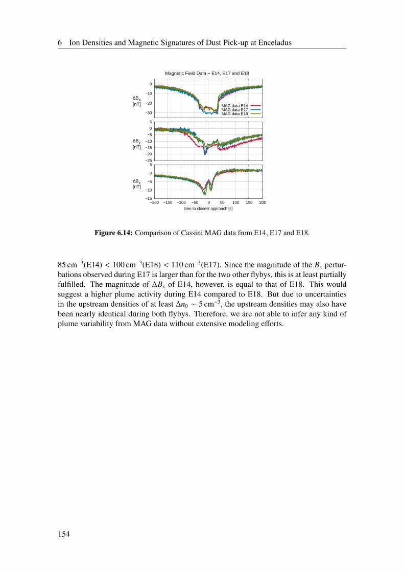
6 Ion Densities and Magnetic Signatures of Dust Pick-up at Enceladus
−30
−20
−10
0
−200 −150 −100 −50 0 50 100 150 200
∆Bx [nT]
Magnetic Field Data − E14, E17 and E18
MAG data E14MAG data E17MAG data E18
−25
−20
−15
−10
−5
0
5
−200 −150 −100 −50 0 50 100 150 200
∆By [nT]
−15
−10
−5
0
5
−200 −150 −100 −50 0 50 100 150 200
time to closest approach [s]
∆Bz [nT]
Figure 6.14: Comparison of Cassini MAG data from E14, E17 and E18.
85 cm−3(E14) < 100 cm−3(E18) < 110 cm−3(E17). Since the magnitude of the Bx pertur-bations observed during E17 is larger than for the two other flybys, this is at least partiallyfulfilled. The magnitude of ∆Bx of E14, however, is equal to that of E18. This wouldsuggest a higher plume activity during E14 compared to E18. But due to uncertaintiesin the upstream densities of at least ∆n0 ∼ 5 cm−3, the upstream densities may also havebeen nearly identical during both flybys. Therefore, we are not able to infer any kind ofplume variability from MAG data without extensive modeling efforts.
154
7 Analysis of Cassini magnetic fieldobservations over the poles of Rhea
The following chapter has been published in wide parts before submission of the thesis.The copyright holder of the pre-publication is the American Geophysical Union, and thecited parts are reprinted with permission. The publication can be found under the follow-ing reference:Simon, S., H. Kriegel, J. Saur, A. Wennmacher, F. M. Neubauer, E. Roussos, U. Motsch-mann, and M. K. Dougherty (2012), Analysis of Cassini magnetic field observations overthe poles of Rhea, Journal of Geophysical Research (Space Physics), 117, A07211, doi:10.1029/2012JA017747
During the first close Rhea flyby (R1 on 26 November 2005), Cassini passed through theplasma wake downstream of the moon at a distance of about 0.7RRH (see figure 2.11).Observations made by MAG during this encounter suggested Rhea to be an electromag-netically inert object that interacts with the impinging magnetospheric plasma mainly byabsorbing the particles incident upon its surface in agreement with section 3.1. Subse-quently, Cassini accomplished the two polar flybys R2 and R3 (see section 2.3.2). Duringboth polar flybys, the Cassini MAG instrument detected significant magnetic field per-turbations inside the Rhea fluxtube, the surface of which is defined by the bundle of fieldlines tangential to the solid body of the moon. While Santolík et al. [2011] applied Cassiniparticle and magnetic field observations to demonstrate the presence of intense plasmawave emissions at the time of the R2 encounter, the origin of the large-scale magneticfield perturbations seen during R2 and R3 has so far not been addressed in the literature.Especially, MAG data from both flybys contain strong perturbations of the flow-alignedmagnetic field component (“draping”). At first glance, this seems untypical for the plasmainteraction of an obstacle that affects the incident magnetospheric plasma mainly by ab-sorbing it (see, e.g. Khurana et al. [2008], Roussos et al. [2008a], Simon et al. [2009a]).Here, we present a detailed analysis of the Cassini magnetic field observations acquiredduring the two polar Rhea flybys R2 and R3. The origin of the observed field perturbationsis discussed, on the one hand, by applying simple analytical models of the interactionbetween an inert moon and the incident flow. On the other hand, we continue the workof Roussos et al. [2008a] and present new hybrid simulations of Rhea’s interaction withthe magnetospheric plasma, taking into account the upstream flow conditions observedduring R2 and R3.
155
7 Analysis of Cassini magnetic field observations over the poles of Rhea
This chapter is organized as follows: in section 2, we classify the interaction betweenRhea and the incident magnetospheric flow. After providing a brief overview of the ambi-ent magnetospheric plasma parameters at Rhea’s L shell (section 2.2), we derive an upperlimit for the contribution of Rhea’s exosphere to the observed magnetic field perturbations(section 7.1). In section 3, we focus on the interpretation of MAG data from R2 and R3. Abrief discussion of the two flyby trajectories (section 2.3.2) is followed by an analysis ofMAG data from the south polar R3 flyby in section 7.2.1 and results from complementaryhybrid simulation runs in section 7.2.2. Our analysis of MAG data from the north-polarR2 encounter is provided in section 7.2.3.
7.1 Magnetic visibility of Rhea’s exosphere
As discussed in section 2.1, INMS data indicate the presence of a tenuous, sputtering-induced atmosphere around Rhea, consisting mainly of molecular oxygen [Teolis et al.2010]. Simultaneously, the Cassini Plasma Spectrometer (CAPS) observed outflowingpositive and negative pick-up ions. However, Khurana et al. [2008] as well as Roussoset al. [2008a] succeeded in explaining MAG data from the first close Rhea encounter(R1) by considering Rhea an electromagnetically inert object that does not possess anatmosphere.One reason for this apparent discrepancy is that the trajectory of the R1 encounter was notsuitable for identifying signatures of a possible gas envelope around Rhea in the magneticfield data. During R1, Cassini passed through Rhea’s plasma wake, with the spacecrafttrajectory being confined to the (z = 0) plane. If a flyby above or below Rhea’s equa-torial plane had been available, the orientation of the measured By perturbations couldhave been employed to clearly discriminate between a mainly plasma-absorbing obsta-cle and an interaction scenario that is dominated by mass/momentum loading (see figure10 in Khurana et al. [2008] and figure 1 in Simon et al. [2009a]). However, for a flybylike R1 that occurred in Rhea’s orbital plane, the By perturbation is almost zero in bothcases (assuming that a possible atmosphere does not possess a pronounced north-southasymmetry).Thus, if Rhea’s atmosphere caused any measurable magnetic field perturbations, the polarflybys R2 and R3 would have been suitable to identify such signatures. However, based onthe parameters provided by Teolis et al. [2010], we expect the gas envelope around Rheato be magnetically invisible even during these close encounters. In order to estimate ifRhea’s exosphere/ionosphere could generate any noticeable magnetic field perturbations,we calculation the interaction strength parameter α (see section 3.2.2) for Rhea.Based on the upstream flow parameters provided in section 2.2, we obtain a value ofΣA = 13.2 S for the Alfvén conductance in the Rhea scenario. An order-of-magnitudeestimate for the Pedersen conductance ΣP can be obtained from the atmospheric parame-ters of Teolis et al. [2010] who derived a total atmospheric O2 content of Ntot = 2.5 · 1029
molecules. For our estimate, we assume the spatial distribution of the neutral gas aroundRhea to be spherically symmetric and to be prescribed by equation 1 in the work of Saurand Strobel [2005], i.e.
156
7.1 Magnetic visibility of Rhea’s exosphere
nn(r) = nn,0
(RRH
r
)2
exp(RRH − r
D
), (7.1)
where r denotes the distance to the center of Rhea. From the work of Saur and Strobel[2005], we adopt a value of D = 100 km for the depletion length scale, while the basedensity n0 can be derived from the total gas content of the atmosphere Ntot according to
nn,0 =Ntot
4πR2RHD
. (7.2)
From the work of Simon et al. [2011a], we adopt a value of κ = 1 · 10−8 cm3/s for thereaction rate between magnetospheric water group ions and oxygen molecules at a relativevelocity of u0 = 40 km/s, considering charge-exchange reactions and elastic collisions.This allows to compute the (effective) ion-neutral collision frequency according to νi(r) =
κnn(r). The ratio of the ion gyrofrequency and the collision frequency is then applied tocompute the local Pedersen conductivity according to
σP(r) =en0
B0·
Ωiνi(r)(
Ωiνi(r)
)2+ 1
, (7.3)
see equation (3.56). By numerically integrating eq. (7.3), we now compute the Pedersenconductance ΣP along a magnetic field line that intersects Rhea at the north pole, i.e.
ΣP,1 =
∫ ∞
r=RRH
σP(r) dr , (7.4)
and along a magnetic field line that is tangential to the solid body of the moon:
ΣP,2 =
∫ ∞
z=0σP
(√z2 + R2
RH
)dz . (7.5)
These two values constitute a lower (ΣP,1) and an upper (ΣP,2) limit for the Pedersen con-ductance in the Rhea scenario, see figure 6 in the work of Neubauer [1998] for illustration.The estimated values of the Pedersen conductance range between ΣP,1 = 0.11 S and ΣP,2 =
0.43 S, respectively, corresponding to an interaction strength of 4.2 ·10−3 ≤ α ≤ 1.6 ·10−2.Thus, the contribution of Rhea’s atmosphere to the magnetic field signatures arising fromthe moon’s interaction with the upstream flow can be considered negligible. The pick-upions generated at Rhea can be treated as test particles that are inserted in a pre-definedelectromagnetic field configuration. For comparison, the parameters provided by Sauret al. [2007] suggest an interaction strength of α = 0.6 for Enceladus’ magnetosphericinteraction. Besides, as will be shown in section 7.2, the key features of the magneticfield observations made during the R2 and R3 flybys can be explained by means of anumerical model that considers only the plasma-absorbing body of Rhea, but not its exo-sphere. Apart from the estimations provided above, the analysis of the magnetic field datatherefore provides independent evidence that Rhea’s exosphere was indeed “magneticallyinvisible” at the times of the R2 and R3 encounters.
157
7 Analysis of Cassini magnetic field observations over the poles of Rhea
We would briefly like to note that Rhea’s exosphere might exhibit some degree of timevariability, similar to what Simon et al. [2011a] found at Dione due to the time-dependencyof energetic particle fluxes in Saturn’s radiation belts. If at certain time periods Rhea’senergetic particle environment is similar to what Voyager 1 saw, then both the atmo-spheric particle content and the associated magnetic field perturbations will be signifi-cantly stronger [Saur and Strobel 2005]. For the conditions of the Voyager 1 flyby, theseauthors derived an interaction strength of α = 0.4. Voyager 1 estimates for the energeticparticle influx to Saturn’s icy satellites showed to be consistently much higher than whathas been measured by Cassini (e.g. Roussos et al. [2008b]), thereby possibly generatingan atmosphere around Rhea that was “magnetically visible” at that time.
7.2 Rhea flybys R2 and R3
In this section, we shall present the Cassini magnetic field observations from the twopolar Rhea encounters. We will commence our discussion with the R3 flyby, since thedata acquired during this passage allow for a much easier depiction of the key features ofthe interaction than the R2 dataset.
7.2.1 Flyby R3: MAG data
The magnetic field signatures observed during R3 are displayed in the right-hand panelsof figure 7.1. The vertical orange lines indicate Cassini’s passages through the surfaceof the Rhea fluxtube
√x2 + y2 = RRH. Although the R3 trajectory was located below
the south pole and did not intersect the moon’s geometric plasma shadow, the magneticfield observations reveal several features immediately indicative of a plasma-absorbingobstacle. The Bz component exhibits a compression signature inside the Rhea fluxtube,i.e. |Bz| is enhanced. Similar enhancements of |Bz| have also been observed in the plasmawakes of Tethys and Dione as well as during the R1 flyby of Rhea [Khurana et al. 2008,Roussos et al. 2008a, Simon et al. 2009a, 2011a]. Such signatures arise from a void in themagnetospheric plasma density due to the absorption of the incident flow at the moon’ssurface. The resulting deficit of plasma pressure is then compensated by an enhancedmagnetic pressure, i.e. the field lines are dragged into the density cavity (see also section3.1). While for the interaction between the Terrestrial moon and the supersonic solarwind, such field compression signatures occur only in the downstream region [Kallio2005], they expand to above and below the poles, if the flow incident upon the obstacle issubsonic. In this case, the bulk speed of the plasma is exceeded by its thermal speed, i.e. asignificant number of particles possess large field-aligned velocities. Therefore, particleswhich were initially located north or south of Rhea can be absorbed as well, yielding anexpansion of the density depletion region to the polar regions of the moon as illustratedin figure 3.1.The compression signature seen in Bz possesses a magnitude of about 2 nT. This valuecan be compared to the maximum field compression expected for the void region of thecentral wake which is (almost) completely evacuated, see figure 3 in the work of Khuranaet al. [2008]. Based on the pressure balance equation
158
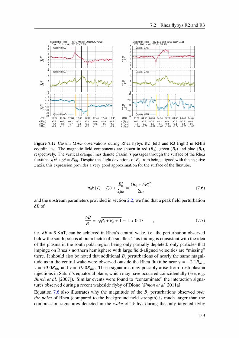
7.2 Rhea flybys R2 and R3
1 2 3 4 5 6 7 8 9
17:34 17:36 17:38 17:40 17:42 17:44 17:46 17:48
Magnetic Field − R2 (2 March 2010 DOY061) C/A: 101 km at UTC 17:40:35
Bx [nT]
Cassini MAG
0
1
2
3
4
17:34 17:36 17:38 17:40 17:42 17:44 17:46 17:48
By [nT]
Cassini MAG
−24−23−22−21−20−19−18−17
17:34 17:36 17:38 17:40 17:42 17:44 17:46 17:48UTCx [RRH]y [RRH]z [RRH]
+0.8−4.4+1.1
+0.5−3.1+1.1
+0.2−1.7+1.1
−0.1−0.4+1.1
−0.4+0.9+1.1
−0.6+2.2+1.1
−0.9+3.5+1.1
−1.2+4.8+1.1
Bz [nT]
Cassini MAG
−2−1 0 1 2 3 4 5
04:4604:4804:5004:5204:5404:5604:5805:00
Magnetic Field − R3 (11 Jan 2011 DOY011) C/A: 70 km at UTC 04:53:25
Bx [nT]
Cassini MAG
−1
0
1
2
3
04:4604:4804:5004:5204:5404:5604:5805:00
By [nT]
Cassini MAG
−23
−22
−21
−20
−19
04:4604:4804:5004:5204:5404:5604:5805:00UTCx [RRH]y [RRH]z [RRH]
+0.9+4.6−1.02
+0.7+3.4−1.03
+0.5+2.1−1.04
+0.4+0.9−1.05
+0.2−0.4−1.06
+0.0−1.6−1.07
−0.2−2.9−1.07
−0.3−4.1−1.08
Bz [nT]
Cassini MAG
Figure 7.1: Cassini MAG observations during Rhea flybys R2 (left) and R3 (right) in RHIScoordinates. The magnetic field components are shown in red (Bx), green (By) and blue (Bz),respectively. The vertical orange lines denote Cassini’s passages through the surface of the Rheafluxtube
√x2 + y2 = RRH . Despite the slight deviations of B0 from being aligned with the negative
z axis, this expression provides a very good approximation for the surface of the fluxtube.
n0k (Ti + Te) +B2
0
2µ0=
(B0 + δB)2
2µ0(7.6)
and the upstream parameters provided in section 2.2, we find that a peak field perturbationδB of
δBB0
=√βi + βe + 1 − 1 ≈ 0.47 , (7.7)
i.e. δB ≈ 9.8 nT, can be achieved in Rhea’s central wake, i.e. the perturbation observedbelow the south pole is about a factor of 5 smaller. This finding is consistent with the ideaof the plasma in the south polar region being only partially depleted: only particles thatimpinge on Rhea’s northern hemisphere with large field-aligned velocities are “missing”there. It should also be noted that additional Bz perturbations of nearly the same magni-tude as in the central wake were observed outside the Rhea fluxtube near y = −2.1RRH,y = +3.0RRH and y = +9.0RRH. These signatures may possibly arise from fresh plasmainjections in Saturn’s equatorial plane, which may have occurred coincidentally (see, e.g.Burch et al. [2007]). Similar events were found to “contaminate” the interaction signa-tures observed during a recent wakeside flyby of Dione [Simon et al. 2011a].Equation 7.6 also illustrates why the magnitude of the Bz perturbations observed overthe poles of Rhea (compared to the background field strength) is much larger than thecompression signatures detected in the wake of Tethys during the only targeted flyby
159
7 Analysis of Cassini magnetic field observations over the poles of Rhea
[Khurana et al. 2008, Simon et al. 2009a]. The above expression can be rewritten as
B0 + δBB0
=√
1 + βi + βe . (7.8)
Hence, the relative magnitude of the maximum field perturbation is determined by thetotal plasma beta of the ambient magnetospheric flow. The more important the impact offlow dynamics, the larger are the compression signatures in the magnetic field. While atRhea, the value of βi + βe is of the order of one, the by far stronger magnetospheric fieldnear Tethys’ orbit (B0 = 167 nT) yields a value of βi + βe = 0.02, thereby allowing for apeak field perturbation of only 1% of the background field (see also Simon et al. [2009a]).The slight enhancement of By observed within the Rhea fluxtube (see figure 7.1) arisesfrom the aforementioned field compression due to plasma absorption. In the (z < 0) halfspace, the field compression yields a region of By < 0 for y < 0 and a region of By > 0 fory > 0, see Simon et al. [2009a]. As can be seen from the (x, y) projection in figure 2.11,Cassini crossed regions of both (y < 0) and (y > 0) while being located inside the Rheafluxtube. Therefore, one would expect the spacecraft to pass through both the (By > 0)and the (By < 0) perturbation region. The fact that only the (By > 0) distortion wasdetected is consistent with CAPS observations from R1 and R1.5 [Wilson et al. 2010],suggesting a slight tilt of the ambient bulk speed away from Saturn. Such a tilt wouldrotate the interaction signatures around the z axis in clockwise direction, thereby shiftingthe region of positive By further into the Rhea fluxtube. The region of (By < 0) was thenprobably missed by Cassini due to the slight tilt of the trajectory. We will address thisfeature again when discussing our hybrid simulation results in section 7.2.2.It is very important to note that Cassini also observed a non-vanishing, positive Bx pertur-bation below Rhea’s south pole, possessing nearly the same magnitude as the perturbationseen in Bz. In general, one would expect such a Bx distortion to arise from field line drap-ing, i.e. from the formation of an Alfvén wing due to an interaction between the obstacle’sionosphere or intrinsic magnetic field and the incident plasma (cf. section 3.2). However,as inferred in section 7.1, Rhea’s gas envelope is far too dilute to cause such strong per-turbations of the magnetospheric field, and the moon was also found to be devoid of aninternal magnetic field by Khurana et al. [2008]. Nonetheless, the observations shownhere suggest that the interaction gives rise to a draping-like broad enhancement in Bx,being comparable to or even stronger than the distortions detected in the Bz and By com-ponents. As will be shown in the following, this Bx enhancement arises from the finiteextension of Rhea’s plasma wake along the corotational flow direction.In contrast to the Terrestrial moon –the wake of which is nearly devoid of plasma even atdistances of several satellite radii [Kallio 2005]–, the wake of a plasma-absorbing moonembedded in a submagnetosonic flow is refilled at rather short distances to the obstacle.As already discussed in section 3.1, the reason for the different refilling of the wake is thehigher sonic Mach number of about MS = 1 for the plasma around Rhea (cf. table 2.4).As demonstrated by preceding hybrid simulations of Rhea’s plasma interaction duringthe R1 flyby (for slightly different upstream parameters than provided in section 2.2, cf.Roussos et al. [2008a]), the number density of the plasma in Rhea’s wake has alreadyreturned to 75% of the background value at a distance (in x direction) of only 1RRH to thesurface of the obstacle. The resulting pressure gradient ∂x p =
∂p∂x ex along the corotation
160
7.2 Rhea flybys R2 and R3
direction gives rise to a diamagnetic current jdia
in (−y) direction,
jdia
=B × ∂x p
B2 ≈B0 × ∂x p
B20
= −1B0
∂p∂x
ey , (7.9)
where B in the first expression denotes the locally perturbed field in the interaction region.As a first approximation, we have assumed the magnetic field B in the expression for j
diato
be equal to the background magnetic field B0 outside the interaction region. As discussedabove, a peak field strength of about 1.5B0 may locally be achieved in Rhea’s centralwake. In the central wake, this would yield an additional factor of 1/1.5 in eq. (7.9).However, this deviation from the background field strength and the associated bending ofthe field lines towards the (y = 0) plane are neglected for the order-of-magnitude estimateof the diamagnetic current provided below. The diamagnetic current j
diais thus parallel
to the convective electric field E0 = −u0 × B0 = −u0B0ey of the undisturbed flow.The orientation of the density gradient as well as the current j
diain the wake and the as-
sociated magnetic field perturbations are illustrated in figure 7.2. This figure shows thatbelow the south pole, the Bx perturbation arising from the diamagnetic current in Rhea’scentral wake is parallel to the positive x axis, whereas above the north pole, the associ-ated Bx perturbation points in negative x direction. Thus, the diamagnetic current arisingfrom the finite length of Rhea’s wake produces field perturbations above the northernand southern poles that are qualitatively similar to what would be expected for field linedraping around a conducting obstacle (cf. red dashed circles in figure 7.2).To demonstrate that the proposed current j
dia∝ −ey can produce a sufficiently strong
magnetic field below the south pole to explain the Bx enhancement observed during R3,let us assume that the thermal pressure p(x) in the wake (note that the contributions ofram and magnetic pressure do not enter the pressure gradient term in the momentumequation of MHD and thus eq. (7.9)) increases linearly from p (x = 1RRH) = 0 at thesurface of Rhea to p (x = 4RRH) = p0 = n0k (Ti + Te) at a distance of 3RRH to the surface.This estimate for the length of the wake is in good agreement with new hybrid modelingresults for Rhea discussed in section 7.2.2. We also verified from the simulations that thepressure gradient term and the Lorentz term indeed make up the dominant contributionsin the momentum equation of the hybrid model within Rhea’s wake.To obtain a simple analytical estimate for the magnetic field associated with the currentjdia, let us further assume that jdia is constant within a cylinder of Radius 1RRH in y di-rection whose axis intersects the x axis at x = 2.5RRH. The circular intersection area ofthis wire with the (x, z) plane covers a large fraction of the density depletion region down-stream of Rhea, see section 3.1. The magnitude δBdia of the magnetic field perturbationoutside the current-carrying region is then given by
δBdia =µ0R2
RH
2√
(x − 2.5RRH)2 + z2·
p0
3B0RRH. (7.10)
This equation follows directly from Ampère’s law by integrating along the circular mag-netic field lines around the cylinder’s axis (along which
∣∣∣δBdia
∣∣∣ is constant), yielding
δBdia =µ0 jdiaπR2
RH
2π√
(x − 2.5RRH)2 + z2. (7.11)
161
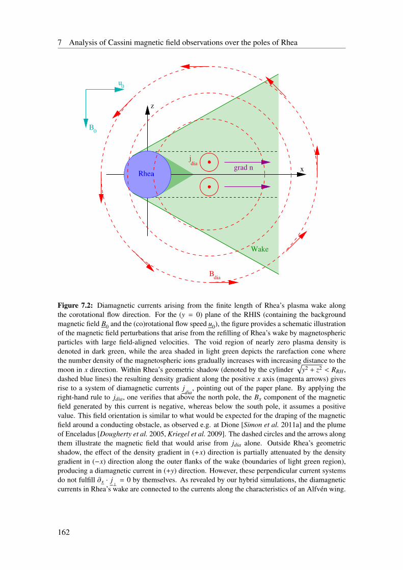
7 Analysis of Cassini magnetic field observations over the poles of Rhea
u0
B0
diaB
jdia
z
x
Wake
grad nRhea
Figure 7.2: Diamagnetic currents arising from the finite length of Rhea’s plasma wake alongthe corotational flow direction. For the (y = 0) plane of the RHIS (containing the backgroundmagnetic field B0 and the (co)rotational flow speed u0), the figure provides a schematic illustrationof the magnetic field perturbations that arise from the refilling of Rhea’s wake by magnetosphericparticles with large field-aligned velocities. The void region of nearly zero plasma density isdenoted in dark green, while the area shaded in light green depicts the rarefaction cone wherethe number density of the magnetospheric ions gradually increases with increasing distance to themoon in x direction. Within Rhea’s geometric shadow (denoted by the cylinder
√y2 + z2 < RRH ,
dashed blue lines) the resulting density gradient along the positive x axis (magenta arrows) givesrise to a system of diamagnetic currents j
dia, pointing out of the paper plane. By applying the
right-hand rule to jdia, one verifies that above the north pole, the Bx component of the magneticfield generated by this current is negative, whereas below the south pole, it assumes a positivevalue. This field orientation is similar to what would be expected for the draping of the magneticfield around a conducting obstacle, as observed e.g. at Dione [Simon et al. 2011a] and the plumeof Enceladus [Dougherty et al. 2005, Kriegel et al. 2009]. The dashed circles and the arrows alongthem illustrate the magnetic field that would arise from jdia alone. Outside Rhea’s geometricshadow, the effect of the density gradient in (+x) direction is partially attenuated by the densitygradient in (−x) direction along the outer flanks of the wake (boundaries of light green region),producing a diamagnetic current in (+y) direction. However, these perpendicular current systemsdo not fulfill ∂x · j
⊥= 0 by themselves. As revealed by our hybrid simulations, the diamagnetic
currents in Rhea’s wake are connected to the currents along the characteristics of an Alfvén wing.
162
7.2 Rhea flybys R2 and R3
In this expression,√
(x − 2.5RRH)2 + z2 denotes the distance from the observer at point(x, y, z) to the axis of the cylinder and
jdia =p0
3B0RRH(7.12)
is the diamagnetic current according to eq. (7.9).Below the south pole (x = 0, z = −1RRH), this yields a perturbation field of about δBdia ≈
0.75 nT, which is of the same order of magnitude as the enhancement of Bx observedwithin the Rhea fluxtube during R3. Hence, we suggest that the Bx perturbations observedbelow Rhea’s south pole mainly arise from currents in the moon’s intermediate wake. Thequestion of how these diamagnetic currents are closed by field-aligned currents will beaddressed in the discussion of our hybrid simulation results in section 7.2.2.However, we would like to point out that this estimation is only meant to demonstrate thata diamagnetic current arising from the finite length of Rhea’s wake is able to produce ameasurable Bx perturbation below the south pole that can in principle explain the observedincrease of Bx. In reality, the geometry of the diamagnetic currents is far more complexthan assumed here. Fully self-consistent hybrid simulations, as discussed in section 7.2.2,are required to determine the precise shape of the current systems in Rhea’s wake and thefield perturbations generated by them.The Rhea interaction scenario is particularly suitable for observing the magnetic fieldperturbations that arise from the finite length of the obstacle’s wake. Although hybridsimulations suggest the extension of Tethys’ plasma wake to be comparable to or evensmaller than the length of Rhea’s wake [Simon et al. 2009a], one would not expect toobserve any strong perturbations of the flow-aligned field component at Tethys. As canbe seen from eq. (7.9), the magnitude of the diamagnetic current is inversely proportionalto the magnetospheric field strength, which at Tethys is almost 8 times larger than at Rhea,yielding a plasma beta of only 0.02 [Khurana et al. 2008, Simon et al. 2009a]. Thus, thecurrent jdia is not expected to make any measurable contributions to the magnetic fielddistortions at Tethys. One should therefore keep in mind that the extension of the wake isnot the only controlling parameter for the magnitude of the diamagnetic current, but themagnetic field plays a key role as well.As demonstrated above, the finite extent of Rhea’s wake along the corotation directionallows for a considerable flow-aligned field perturbation. However, as can also be seenfrom figure 7.2, such a flow-aligned perturbation may occur only outside the (z = 0)plane. Within the (z = 0) plane, it leads to a field-aligned perturbation (i.e. δB ∝ ez) thatstrengthens the field upstream and decreases it downstream. The downstream decrease isprobably obscured by the enhancement due to reduced plasma pressure. Upstream, theperturbation is without “competition” and should show an enhancement signature, as itwould also be caused by mass/momentum loading (e.g. Kriegel et al. [2009], Simon et al.[2011a]).As can also be seen from figure 7.2, the density gradient along the outer flanks of theinteraction region (boundaries of the light green cone) possesses a component in negativex direction. Thus, it generates a diamagnetic current in positive y direction and a magneticfield that counteracts the effects of the finite wake extension along the corotation direction.In order for the Bx perturbation below the south pole to become positive (as observed
163
7 Analysis of Cassini magnetic field observations over the poles of Rhea
during R3), the effect caused by the currents at the outer flanks of the wake must beovercompensated by the field arising from the density gradient in (+x) direction in thecentral wake. This is especially important in the polar regions where the wake flanks“touch” the solid body of the moon, cf. figure 7.2. While outside Rhea’s geometricshadow, i. e. at
√y2 + z2 > RRH (and x > 1RRH), density gradients in (+x) and (−x)
direction occur, the density gradient inside the shadow region points exclusively in (+x)direction and may even cause strong field perturbations above Rhea’s poles. Numericalsimulations (see section 7.2.2) are required to understand the magnetic field distortionscaused by this complex system of wakeside currents.Finally, we would briefly like to note that the field perturbations seen in By and Bz are alsocaused by a diamagnetic current system, arising from the finite extension of the densitycavity in y direction [Colburn et al. 1967]. In the (y > 0) half space, the pressure gradientpoints in (+y) direction, i.e. the resulting diamagnetic current is parallel to ex. In the(y < 0) half space, the directions of both the density gradient and the resulting currentare reversed. By applying the right-hand rule to these two current systems, one can easilyverify that they are responsible for enhancing |Bz| in the central wake and depressingthe field at the flanks of the interaction region. They are also responsible for generatingthe quadrupolar pattern of different By orientations illustrated in figure 1 of Simon et al.[2009a]. The diamagnetic currents in x direction are closed within a current loop aroundthe ramside of the satellite (see figure 11.8 in Mauk et al. [2009]).
7.2.2 Flyby R3: Hybrid simulations
So far, our analysis of the R3 magnetic field observations is mainly based on analyticalestimates of the effects generating the perturbation signatures. In this way, we have beenable to explain numerous features seen in the dataset. However, to confirm that our in-terpretation is quantitatively realistic and to gain further insights into the current systemsarising from the finite length of the wake –especially how jdia is closed–, the interactionneeds to be treated within the framework of a fully self-consistent plasma simulation. Inaddition, there is one feature in the R3 dataset which has not yet been addressed: coinci-dent with Cassini’s outbound passage (y < 0) through the surface of the Rhea fluxtube, themagnetometer detected a sharply pronounced dip in the Bx component with a magnitudeof δBx ≈ −2.1 nT, i.e. comparable to the strength of the Bx enhancement seen within theRhea fluxtube.To clarify these remaining issues, we carry out new simulations of Rhea’s magnetosphericinteraction, amplifying the pilot study by Roussos et al. [2008a]. Since the hybrid codetreats the ions as individual particles, it is particularly suitable for reproducing effectsassociated with finite ion gyroradii, especially asymmetries in the flow deflection patternand non-Maxwellian particle distribution functions (e.g., the ring distributions associatedwith ion pick-up or the counter-stream distribution in the wake of an inert moon, cf. Simonet al. [2009a]).Since the key features and basic equations of this code have been elaborated on in detailin chapter 4, we shall provide only a brief discussion of how the code is adapted to theRhea scenario.
164
7.2 Rhea flybys R2 and R3
7.2.2.1 Model description and input parameters
The magnetospheric upstream conditions applied in the simulations are provided in sec-tion 2.2. For the simulation of R3, however, three slight adjustments have been included:first, the weak tilt of the background magnetic field with respect to the z axis (see upper-right panel of figure 7.1) has been taken into account and we set B0 = (1.8, 0.6,−20.8) nT,i.e. the magnitude is again B0 ≈ 21 nT. Second, the upstream plasma density observedduring R3 was also slightly larger than the value of n0 = 6 cm−3 derived by Wilson et al.[2010] for R1 and R1.5. Measurements of Cassini’s Radio and Plasma Wave Science In-strument suggest a value of n0 = 7 cm−3 [Roussos et al. 2012], which we adopt as inputparameter for our model. Third, while data from the R1 flyby [Wilson et al. 2010] suggestan ion temperature of about kTi = 200 eV, we achieved better agreement between simula-tion and MAG data for R3 by applying a value of kTi = 100 eV, as proposed by Roussoset al. [2008a]. At the time of this writing, no measurements of the ion temperature wereavailable for the R3 encounter. For this reason, we have used the ion temperature as a freeparameter (within the range of values provided by Wilson et al. [2010], Khurana et al.[2008] and Roussos et al. [2008a]) to achieve best possible agreement between simula-tion and magnetic field data. An overview about the used parameters is provided in table7.1. The applied value of kTi yields an ion gyroradius of rg = 0.45RRH. The modified up-stream conditions yield an only slightly increased Alfvénic Mach number of MA = 0.95and a magnetosonic Mach number of MMS = 0.73. While these changes have negligiblequalitative influence on the overall structures seen in the simulations, they may nonethe-less strongly affect the magnitudes of the signatures. The minor hydrogen componentidentified in CAPS ion data from R1 and R1.5 by Wilson et al. [2010] is not included inour simulations.As discussed in sections 3.1 and 4.5.1, Rhea is treated as an electromagnetically inertand plasma-absorbing body, i.e. the tenuous atmosphere described by Teolis et al. [2010]is not included. The simulation applies a hierarchical Cartesian grid with three differentrefinement levels. The extent and location of these levels is shown in figure 7.3. At thehighest level, a peak resolution of 0.05RRH is achieved near the surface of the moon. Thecell size in the other two levels is two/four times larger. The simulation domain is cubic,possessing an extension of −5RRH ≤ x ≤ +10RRH and −7.5RRH ≤ y, z ≤ +7.5RRH.
7.2.2.2 Discussion of simulation results
The results of our hybrid simulations can be seen in figures 7.4, 7.5 and 7.6, respec-tively. Panels (a) and (b) of figure 7.4 display the magnetospheric plasma density and thecorresponding Bx perturbation in the (z = 0) plane of the RHIS. For a downstream cutthrough the wake at x = 2RRH, panels (c) and (d) show the distortions of the Bx and By
components.To explore the influence of the large ion gyroradii on the signatures seen in panels (c)and (d), the final row of figure 7.4 displays results from a test simulation where the radiusof Rhea has been artificially increased by a factor of 3, while the incident flow param-eters were left unchanged. Thus, the ion gyroradius is now rg = 0.15R, where R is theradius of the artificially enlarged obstacle. The purpose of this test scenario is to isolate
165
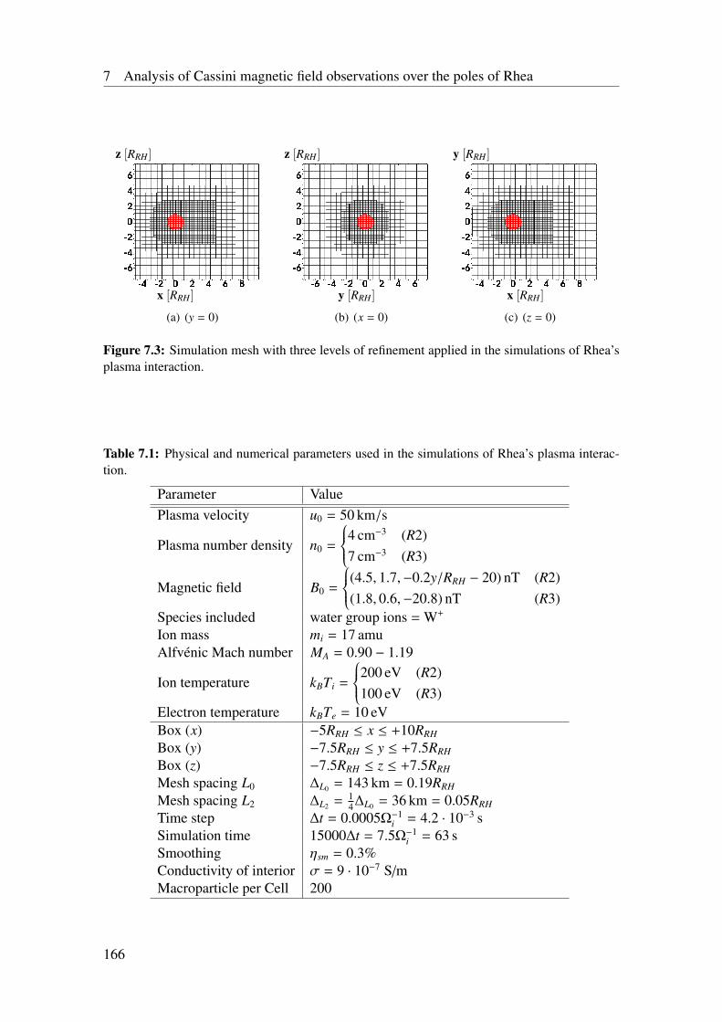
7 Analysis of Cassini magnetic field observations over the poles of Rhea
x [RRH]
z [RRH]
1
(a) (y = 0)
y [RRH]
z [RRH]
1
(b) (x = 0)
x [RRH]
y [RRH]
1
(c) (z = 0)
Figure 7.3: Simulation mesh with three levels of refinement applied in the simulations of Rhea’splasma interaction.
Table 7.1: Physical and numerical parameters used in the simulations of Rhea’s plasma interac-tion.
Parameter ValuePlasma velocity u0 = 50 km/s
Plasma number density n0 =
4 cm−3 (R2)7 cm−3 (R3)
Magnetic field B0 =
(4.5, 1.7,−0.2y/RRH − 20) nT (R2)(1.8, 0.6,−20.8) nT (R3)
Species included water group ions = W+
Ion mass mi = 17 amuAlfvénic Mach number MA = 0.90 − 1.19
Ion temperature kBTi =
200 eV (R2)100 eV (R3)
Electron temperature kBTe = 10 eVBox (x) −5RRH ≤ x ≤ +10RRH
Box (y) −7.5RRH ≤ y ≤ +7.5RRH
Box (z) −7.5RRH ≤ z ≤ +7.5RRH
Mesh spacing L0 ∆L0 = 143 km = 0.19RRH
Mesh spacing L2 ∆L2 = 14∆L0 = 36 km = 0.05RRH
Time step ∆t = 0.0005Ω−1i = 4.2 · 10−3 s
Simulation time 15000∆t = 7.5Ω−1i = 63 s
Smoothing ηsm = 0.3%Conductivity of interior σ = 9 · 10−7 S/mMacroparticle per Cell 200
166
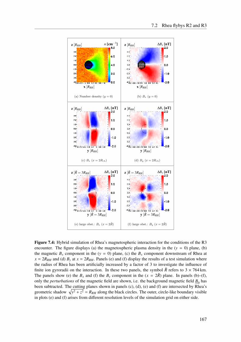
7.2 Rhea flybys R2 and R3
x [RRH]
z [RRH] n [cm−3]
1(a) Number density (y = 0)
x [RRH]
z [RRH] ∆Bx [nT]
1(b) Bx (y = 0)
y [RRH]
z [RRH] ∆Bx [nT]
1(c) Bx (x = 2Rrh)
y [RRH]
z [RRH] ∆By [nT]
1(d) By (x = 2Rrh)
y [R = 3RRH]
z [R = 3RRH] ∆Bx [nT]
1(e) large obst.: Bx (x = 2R)
y [R = 3RRH]
z [R = 3RRH] ∆By [nT]
1(f) large obst.: By (x = 2R)
Figure 7.4: Hybrid simulation of Rhea’s magnetospheric interaction for the conditions of the R3encounter. The figure displays (a) the magnetospheric plasma density in the (y = 0) plane, (b)the magnetic Bx component in the (y = 0) plane, (c) the Bx component downstream of Rhea atx = 2RRH and (d) By at x = 2RRH . Panels (e) and (f) display the results of a test simulation wherethe radius of Rhea has been artificially increased by a factor of 3 to investigate the influence offinite ion gyroradii on the interaction. In these two panels, the symbol R refers to 3 × 764 km.The panels show (e) the Bx and (f) the By component in the (x = 2R) plane. In panels (b)–(f),only the perturbations of the magnetic field are shown, i.e. the background magnetic field B0 hasbeen subtracted. The cutting planes shown in panels (c), (d), (e) and (f) are intersected by Rhea’sgeometric shadow
√y2 + z2 = RRH along the black circles. The outer, circle-like boundary visible
in plots (e) and (f) arises from different resolution levels of the simulation grid on either side.
167
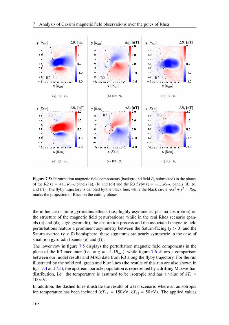
7 Analysis of Cassini magnetic field observations over the poles of Rhea
CCCO
R2
x [RRH]
y [RRH] ∆Bx [nT]
1(a) R2: Bx
CCCO
R2
x [RRH]
y [RRH] ∆By [nT]
1(b) R2: By
CCCO
R2
x [RRH]
y [RRH] ∆Bz [nT]
1(c) R2: Bz
R3
x [RRH]
y [RRH] ∆Bx [nT]
1(d) R3: Bx
R3
x [RRH]
y [RRH] ∆By [nT]
1(e) R3: By
R3
x [RRH]
y [RRH] ∆Bz [nT]
1(f) R3: Bz
Figure 7.5: Perturbation magnetic field components (background field B0 subtracted) in the planesof the R2 (z = +1.1RRH , panels (a), (b) and (c)) and the R3 flyby (z = −1.1RRH , panels (d), (e)and (f)). The flyby trajectory is denoted by the black line, while the black circle
√x2 + y2 = RRH
marks the projection of Rhea on the cutting planes.
the influence of finite gyroradius effects (i.e., highly asymmetric plasma absorption) onthe structure of the magnetic field perturbations: while in the real Rhea scenario (pan-els (c) and (d), large gyroradii), the absorption process and the associated magnetic fieldperturbations feature a prominent asymmetry between the Saturn-facing (y > 0) and theSaturn-averted (y < 0) hemisphere, these signatures are nearly symmetric in the case ofsmall ion gyroradii (panels (e) and (f)).The lower row in figure 7.5 displays the perturbation magnetic field components in theplane of the R3 encounter (i.e. at z = −1.1RRH), while figure 7.6 shows a comparisonbetween our model results and MAG data from R3 along the flyby trajectory. For the runillustrated by the solid red, green and blue lines (the results of this run are also shown infigs. 7.4 and 7.5), the upstream particle population is represented by a drifting Maxwelliandistribution, i.e. the temperature is assumed to be isotropic and has a value of kTi =
100 eV.In addition, the dashed lines illustrate the results of a test scenario where an anisotropicion temperature has been included (kTi,⊥ = 150 eV, kTi,‖ = 50 eV). The applied values
168
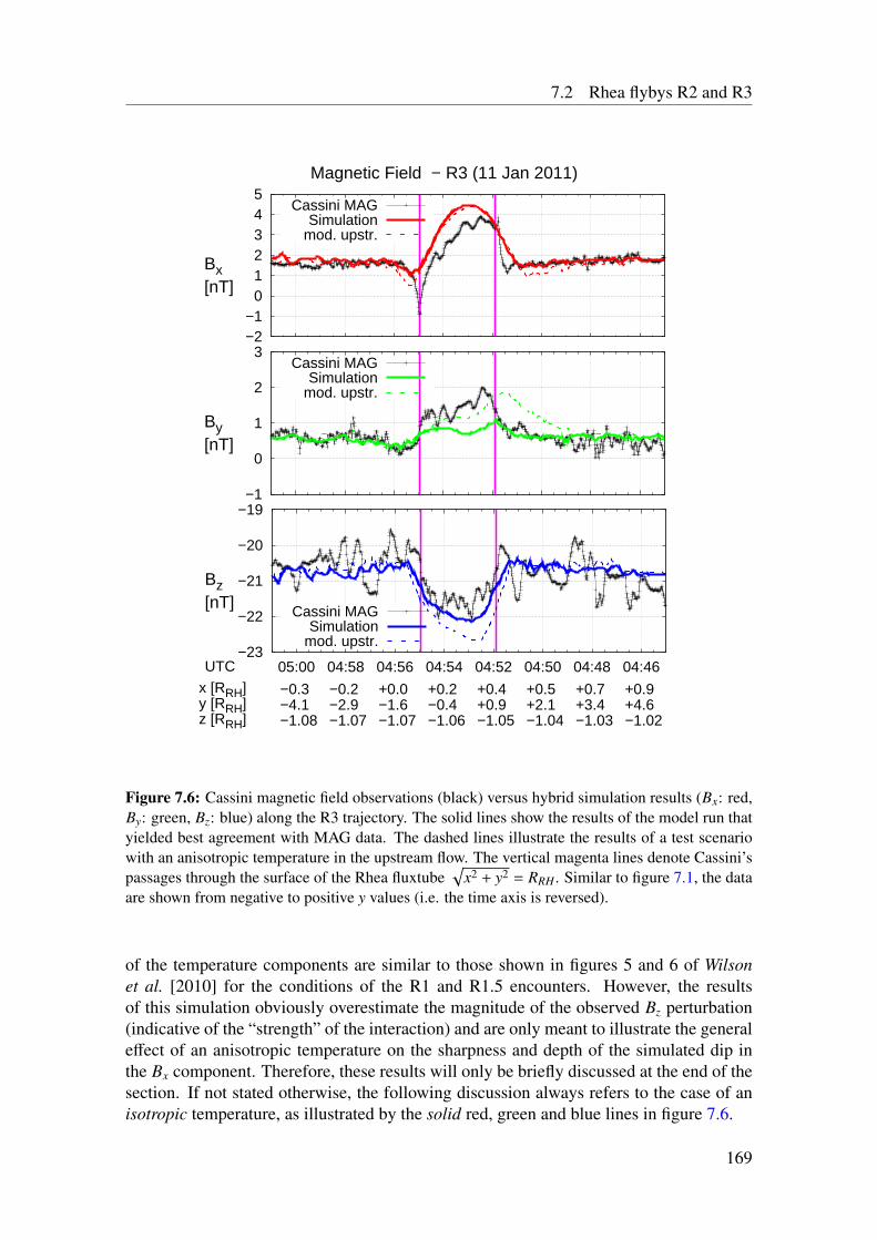
7.2 Rhea flybys R2 and R3
−2−1 0 1 2 3 4 5
04:4604:4804:5004:5204:5404:5604:5805:00
Magnetic Field − R3 (11 Jan 2011)
Bx [nT]
Cassini MAGSimulation
mod. upstr.
−1
0
1
2
3
04:4604:4804:5004:5204:5404:5604:5805:00
By [nT]
Cassini MAGSimulation
mod. upstr.
−23
−22
−21
−20
−19
04:4604:4804:5004:5204:5404:5604:5805:00UTCx [RRH]y [RRH]z [RRH]
+0.9+4.6−1.02
+0.7+3.4−1.03
+0.5+2.1−1.04
+0.4+0.9−1.05
+0.2−0.4−1.06
+0.0−1.6−1.07
−0.2−2.9−1.07
−0.3−4.1−1.08
Bz [nT] Cassini MAG
Simulationmod. upstr.
Figure 7.6: Cassini magnetic field observations (black) versus hybrid simulation results (Bx: red,By: green, Bz: blue) along the R3 trajectory. The solid lines show the results of the model run thatyielded best agreement with MAG data. The dashed lines illustrate the results of a test scenariowith an anisotropic temperature in the upstream flow. The vertical magenta lines denote Cassini’spassages through the surface of the Rhea fluxtube
√x2 + y2 = RRH . Similar to figure 7.1, the data
are shown from negative to positive y values (i.e. the time axis is reversed).
of the temperature components are similar to those shown in figures 5 and 6 of Wilsonet al. [2010] for the conditions of the R1 and R1.5 encounters. However, the resultsof this simulation obviously overestimate the magnitude of the observed Bz perturbation(indicative of the “strength” of the interaction) and are only meant to illustrate the generaleffect of an anisotropic temperature on the sharpness and depth of the simulated dip inthe Bx component. Therefore, these results will only be briefly discussed at the end of thesection. If not stated otherwise, the following discussion always refers to the case of anisotropic temperature, as illustrated by the solid red, green and blue lines in figure 7.6.
169
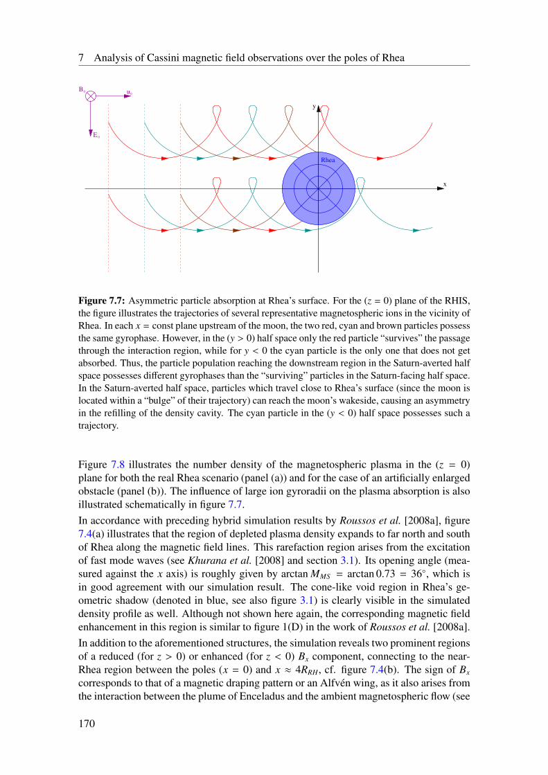
7 Analysis of Cassini magnetic field observations over the poles of Rhea
u00B
0E
y
x
Rhea
Figure 7.7: Asymmetric particle absorption at Rhea’s surface. For the (z = 0) plane of the RHIS,the figure illustrates the trajectories of several representative magnetospheric ions in the vicinity ofRhea. In each x = const plane upstream of the moon, the two red, cyan and brown particles possessthe same gyrophase. However, in the (y > 0) half space only the red particle “survives” the passagethrough the interaction region, while for y < 0 the cyan particle is the only one that does not getabsorbed. Thus, the particle population reaching the downstream region in the Saturn-averted halfspace possesses different gyrophases than the “surviving” particles in the Saturn-facing half space.In the Saturn-averted half space, particles which travel close to Rhea’s surface (since the moon islocated within a “bulge” of their trajectory) can reach the moon’s wakeside, causing an asymmetryin the refilling of the density cavity. The cyan particle in the (y < 0) half space possesses such atrajectory.
Figure 7.8 illustrates the number density of the magnetospheric plasma in the (z = 0)plane for both the real Rhea scenario (panel (a)) and for the case of an artificially enlargedobstacle (panel (b)). The influence of large ion gyroradii on the plasma absorption is alsoillustrated schematically in figure 7.7.In accordance with preceding hybrid simulation results by Roussos et al. [2008a], figure7.4(a) illustrates that the region of depleted plasma density expands to far north and southof Rhea along the magnetic field lines. This rarefaction region arises from the excitationof fast mode waves (see Khurana et al. [2008] and section 3.1). Its opening angle (mea-sured against the x axis) is roughly given by arctan MMS = arctan 0.73 = 36, which isin good agreement with our simulation result. The cone-like void region in Rhea’s ge-ometric shadow (denoted in blue, see also figure 3.1) is clearly visible in the simulateddensity profile as well. Although not shown here again, the corresponding magnetic fieldenhancement in this region is similar to figure 1(D) in the work of Roussos et al. [2008a].In addition to the aforementioned structures, the simulation reveals two prominent regionsof a reduced (for z > 0) or enhanced (for z < 0) Bx component, connecting to the near-Rhea region between the poles (x = 0) and x ≈ 4RRH, cf. figure 7.4(b). The sign of Bx
corresponds to that of a magnetic draping pattern or an Alfvén wing, as it also arises fromthe interaction between the plume of Enceladus and the ambient magnetospheric flow (see
170
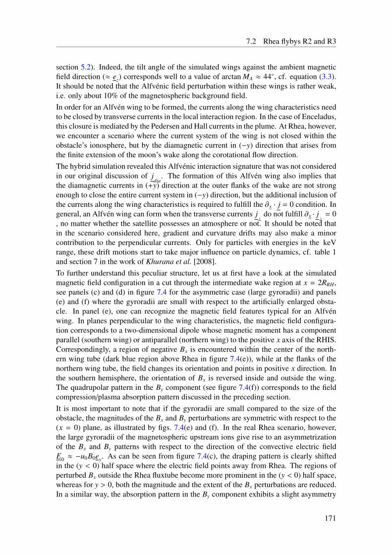
7.2 Rhea flybys R2 and R3
section 5.2). Indeed, the tilt angle of the simulated wings against the ambient magneticfield direction (≈ ez) corresponds well to a value of arctan MA ≈ 44, cf. equation (3.3).It should be noted that the Alfvénic field perturbation within these wings is rather weak,i.e. only about 10% of the magnetospheric background field.In order for an Alfvén wing to be formed, the currents along the wing characteristics needto be closed by transverse currents in the local interaction region. In the case of Enceladus,this closure is mediated by the Pedersen and Hall currents in the plume. At Rhea, however,we encounter a scenario where the current system of the wing is not closed within theobstacle’s ionosphere, but by the diamagnetic current in (−y) direction that arises fromthe finite extension of the moon’s wake along the corotational flow direction.The hybrid simulation revealed this Alfvénic interaction signature that was not consideredin our original discussion of j
dia. The formation of this Alfvén wing also implies that
the diamagnetic currents in (+y) direction at the outer flanks of the wake are not strongenough to close the entire current system in (−y) direction, but the additional inclusion ofthe currents along the wing characteristics is required to fulfill the ∂x · j = 0 condition. Ingeneral, an Alfvén wing can form when the transverse currents j
⊥do not fulfill ∂x · j
⊥= 0
, no matter whether the satellite possesses an atmosphere or not. It should be noted thatin the scenario considered here, gradient and curvature drifts may also make a minorcontribution to the perpendicular currents. Only for particles with energies in the keVrange, these drift motions start to take major influence on particle dynamics, cf. table 1and section 7 in the work of Khurana et al. [2008].To further understand this peculiar structure, let us at first have a look at the simulatedmagnetic field configuration in a cut through the intermediate wake region at x = 2RRH,see panels (c) and (d) in figure 7.4 for the asymmetric case (large gyroradii) and panels(e) and (f) where the gyroradii are small with respect to the artificially enlarged obsta-cle. In panel (e), one can recognize the magnetic field features typical for an Alfvénwing. In planes perpendicular to the wing characteristics, the magnetic field configura-tion corresponds to a two-dimensional dipole whose magnetic moment has a componentparallel (southern wing) or antiparallel (northern wing) to the positive x axis of the RHIS.Correspondingly, a region of negative Bx is encountered within the center of the north-ern wing tube (dark blue region above Rhea in figure 7.4(e)), while at the flanks of thenorthern wing tube, the field changes its orientation and points in positive x direction. Inthe southern hemisphere, the orientation of Bx is reversed inside and outside the wing.The quadrupolar pattern in the By component (see figure 7.4(f)) corresponds to the fieldcompression/plasma absorption pattern discussed in the preceding section.It is most important to note that if the gyroradii are small compared to the size of theobstacle, the magnitudes of the Bx and By perturbations are symmetric with respect to the(x = 0) plane, as illustrated by figs. 7.4(e) and (f). In the real Rhea scenario, however,the large gyroradii of the magnetospheric upstream ions give rise to an asymmetrizationof the Bx and By patterns with respect to the direction of the convective electric fieldE0 ≈ −u0B0ey. As can be seen from figure 7.4(c), the draping pattern is clearly shiftedin the (y < 0) half space where the electric field points away from Rhea. The regions ofperturbed Bx outside the Rhea fluxtube become more prominent in the (y < 0) half space,whereas for y > 0, both the magnitude and the extent of the Bx perturbations are reduced.In a similar way, the absorption pattern in the By component exhibits a slight asymmetry
171
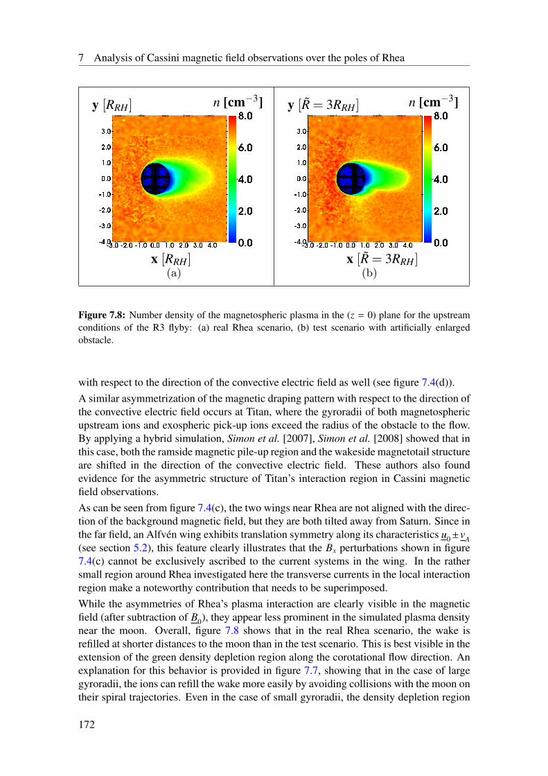
7 Analysis of Cassini magnetic field observations over the poles of Rhea
x [RRH]
y [RRH] n [cm−3]
1
(a)x [R = 3RRH]
y [R = 3RRH] n [cm−3]
1
(b)
Figure 7.8: Number density of the magnetospheric plasma in the (z = 0) plane for the upstreamconditions of the R3 flyby: (a) real Rhea scenario, (b) test scenario with artificially enlargedobstacle.
with respect to the direction of the convective electric field as well (see figure 7.4(d)).A similar asymmetrization of the magnetic draping pattern with respect to the direction ofthe convective electric field occurs at Titan, where the gyroradii of both magnetosphericupstream ions and exospheric pick-up ions exceed the radius of the obstacle to the flow.By applying a hybrid simulation, Simon et al. [2007], Simon et al. [2008] showed that inthis case, both the ramside magnetic pile-up region and the wakeside magnetotail structureare shifted in the direction of the convective electric field. These authors also foundevidence for the asymmetric structure of Titan’s interaction region in Cassini magneticfield observations.As can be seen from figure 7.4(c), the two wings near Rhea are not aligned with the direc-tion of the background magnetic field, but they are both tilted away from Saturn. Since inthe far field, an Alfvén wing exhibits translation symmetry along its characteristics u0±vA(see section 5.2), this feature clearly illustrates that the Bx perturbations shown in figure7.4(c) cannot be exclusively ascribed to the current systems in the wing. In the rathersmall region around Rhea investigated here the transverse currents in the local interactionregion make a noteworthy contribution that needs to be superimposed.While the asymmetries of Rhea’s plasma interaction are clearly visible in the magneticfield (after subtraction of B0), they appear less prominent in the simulated plasma densitynear the moon. Overall, figure 7.8 shows that in the real Rhea scenario, the wake isrefilled at shorter distances to the moon than in the test scenario. This is best visible in theextension of the green density depletion region along the corotational flow direction. Anexplanation for this behavior is provided in figure 7.7, showing that in the case of largegyroradii, the ions can refill the wake more easily by avoiding collisions with the moon ontheir spiral trajectories. Even in the case of small gyroradii, the density depletion region
172
7.2 Rhea flybys R2 and R3
features a slight asymmetry. The occurrence of this effect is consistent with our precedingsimulations of Tethys’ magnetospheric interaction and arises from the Hall term [Simonet al. 2009a]. In the real Rhea scenario, this effect is still present (visible in the outerboundary of the green region in figure 7.8(a)), although the outer flanks of the wake aremore blurred. However, comparing the locations of the central density void downstreamof the moon (dark blue region) between the real Rhea scenario (cf. figure 7.8(a)) andthe case of an artificially enlarged obstacle (cf. figure 7.8(b)) also shows that in the realscenario, the central density void is more prominent in the Saturn-averted half space wherethe convective electric field points away from Rhea. This effect may give rise to a slightlysteeper density profile (along the corotation direction) for y < 0 than in the test scenario,generating a stronger diamagnetic current in the Saturn-averted half space and therebycontributing to the asymmetry in the magnetic field pattern. Given the weakness of thesevisible modifications in the density profile (compared to the background density), it isalso important to notice that the change in the magnitude of the Bx perturbation in the(y < 0) half space between asymmetric and symmetric case (figure 7.4(c) versus 7.4(e))is on the order of only 1 nT, i.e. less than 5% of the background field.Based on these results, we can now investigate the origin of the spiky dip in Bx detectedby Cassini when leaving the Rhea fluxtube (y < 0). As can be seen from figure 7.5(d),Cassini only grazed the weakly pronounced region of reduced Bx in the inbound regionof R3 (y > 0). However, after leaving the Rhea fluxtube where Bx was enhanced, thespacecraft passed through the more prominent region of reduced Bx in the (y < 0) halfspace. A comparison between measured and simulated Bx component (see upper panelof figure 7.6) shows that our simulation result is in good agreement with the measuredBx signature. Especially, both the magnitude and the width of the Bx enhancement insidethe Rhea fluxtube are quantitatively reproduced by the simulation. The location of the Bx
dip at the (y < 0) surface of the Rhea fluxtube is reproduced by the simulation as well,but its magnitude and sharpness are underestimated. A possible reason for this may bethe finite level of numerical diffusion in the simulations or the occurrence of effects onelectron scales which are not covered by the hybrid model. However, it is important tonotice that our model qualitatively reproduces this dip by considering plasma-absorptionat the moon’s surface alone.To further illustrate that the effect producing the Bx spike seems to be reproduced bythe hybrid simulation, let us have a brief look at the results of the test scenario with ananisotropic temperature (dashed red, green and blue lines in figure 7.6). This run overesti-mates the width of the enhancement in By and especially the compression signature in Bz.Due to the increased perpendicular temperature (150 eV versus 100 eV), the pressure lossat Rhea’s surface is larger than in the first simulation run, therefore requiring a strongermagnetic field enhancement.However, this run also produces a more prominent spike at the (y < 0) flank of the Rheafluxtube. These results illustrate that although the global features of the interaction re-main qualitatively unaffected by the modified temperature, the magnitudes of the simu-lated magnetic field signatures are highly sensitive to the incident magnetospheric flowconditions. To a high degree, the discrepancy between simulation and measurement nearthe (y < 0) passage through the Rhea fluxtube may probably be ascribed to uncertaintiesin the ambient flow conditions. Of course, we cannot definitely exclude that additional
173
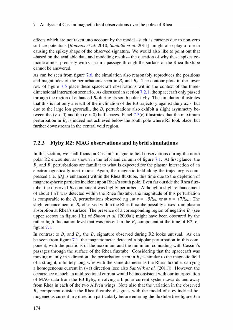
7 Analysis of Cassini magnetic field observations over the poles of Rhea
effects which are not taken into account by the model –such as currents due to non-zerosurface potentials [Roussos et al. 2010, Santolík et al. 2011]– might also play a role incausing the spikey shape of the observed signature. We would also like to point out that–based on the available data and modeling results– the question of why these spikes co-incide almost precisely with Cassini’s passage through the surface of the Rhea fluxtubecannot be answered.As can be seen from figure 7.6, the simulation also reasonably reproduces the positionsand magnitudes of the perturbations seen in By and Bz. The contour plots in the lowerrow of figure 7.5 place these spacecraft observations within the context of the three-dimensional interaction scenario. As discussed in section 7.2.1, the spacecraft only passedthrough the region of enhanced By during its south polar flyby. The simulation illustratesthat this is not only a result of the inclination of the R3 trajectory against the y axis, butdue to the large ion gyroradii, the By perturbations also exhibit a slight asymmetry be-tween the (y > 0) and the (y < 0) half spaces. Panel 7.5(c) illustrates that the maximumperturbation in Bz is indeed not achieved below the south pole where R3 took place, butfurther downstream in the central void region.
7.2.3 Flyby R2: MAG observations and hybrid simulations
In this section, we shall focus on Cassini’s magnetic field observations during the northpolar R2 encounter, as shown in the left-hand column of figure 7.1. At first glance, theBy and Bz perturbations are familiar to what is expected for the plasma interaction of anelectromagnetically inert moon. Again, the magnetic field along the trajectory is com-pressed (i.e. |Bz| is enhanced) within the Rhea fluxtube, this time due to the depletion ofmagnetospheric particles incident upon Rhea’s south pole. Even far outside the Rhea flux-tube, the observed By component was highly perturbed. Although a slight enhancementof about 1 nT was detected within the Rhea fluxtube, the magnitude of this perturbationis comparable to the By perturbations observed e.g., at y = −5RRH or at y = +7RRH. Theslight enhancement of By observed within the Rhea fluxtube possibly arises from plasmaabsorption at Rhea’s surface. The presence of a corresponding region of negative By (seeupper sectors in figure 1(ii) of Simon et al. [2009a]) might have been obscured by therather high fluctuation level that was present in the By component at the time of R2, cf.figure 7.1.In contrast to By and Bz, the Bx signature observed during R2 looks unusual. As canbe seen from figure 7.1, the magnetometer detected a bipolar perturbation in this com-ponent, with the positions of the maximum and the minimum coinciding with Cassini’spassages through the surface of the Rhea fluxtube. Considering that the spacecraft wasmoving mainly in y direction, the perturbation seen in Bx is similar to the magnetic fieldof a straight, infinitely long wire with the same diameter as the Rhea fluxtube, carryinga homogeneous current in (+z) direction (see also Santolík et al. [2011]). However, theoccurrence of such an unidirectional current would be inconsistent with our interpretationof MAG data from the R3 flyby, involving a bipolar current system towards and awayfrom Rhea in each of the two Alfvén wings. Note also that the variation in the observedBx component outside the Rhea fluxtube disagrees with the model of a cylindrical ho-mogeneous current in z direction particularly before entering the fluxtube (see figure 3 in
174
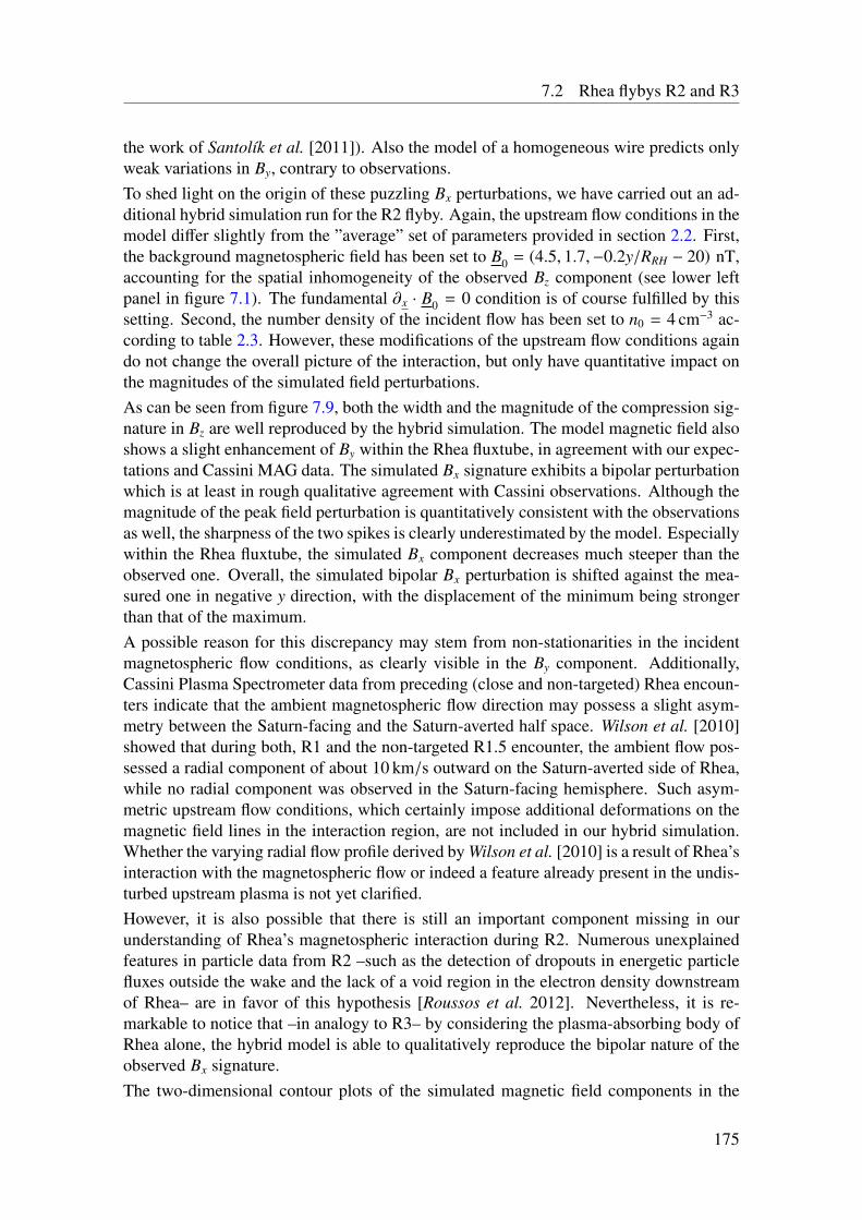
7.2 Rhea flybys R2 and R3
the work of Santolík et al. [2011]). Also the model of a homogeneous wire predicts onlyweak variations in By, contrary to observations.To shed light on the origin of these puzzling Bx perturbations, we have carried out an ad-ditional hybrid simulation run for the R2 flyby. Again, the upstream flow conditions in themodel differ slightly from the ”average” set of parameters provided in section 2.2. First,the background magnetospheric field has been set to B0 = (4.5, 1.7,−0.2y/RRH − 20) nT,accounting for the spatial inhomogeneity of the observed Bz component (see lower leftpanel in figure 7.1). The fundamental ∂x · B0 = 0 condition is of course fulfilled by thissetting. Second, the number density of the incident flow has been set to n0 = 4 cm−3 ac-cording to table 2.3. However, these modifications of the upstream flow conditions againdo not change the overall picture of the interaction, but only have quantitative impact onthe magnitudes of the simulated field perturbations.As can be seen from figure 7.9, both the width and the magnitude of the compression sig-nature in Bz are well reproduced by the hybrid simulation. The model magnetic field alsoshows a slight enhancement of By within the Rhea fluxtube, in agreement with our expec-tations and Cassini MAG data. The simulated Bx signature exhibits a bipolar perturbationwhich is at least in rough qualitative agreement with Cassini observations. Although themagnitude of the peak field perturbation is quantitatively consistent with the observationsas well, the sharpness of the two spikes is clearly underestimated by the model. Especiallywithin the Rhea fluxtube, the simulated Bx component decreases much steeper than theobserved one. Overall, the simulated bipolar Bx perturbation is shifted against the mea-sured one in negative y direction, with the displacement of the minimum being strongerthan that of the maximum.A possible reason for this discrepancy may stem from non-stationarities in the incidentmagnetospheric flow conditions, as clearly visible in the By component. Additionally,Cassini Plasma Spectrometer data from preceding (close and non-targeted) Rhea encoun-ters indicate that the ambient magnetospheric flow direction may possess a slight asym-metry between the Saturn-facing and the Saturn-averted half space. Wilson et al. [2010]showed that during both, R1 and the non-targeted R1.5 encounter, the ambient flow pos-sessed a radial component of about 10 km/s outward on the Saturn-averted side of Rhea,while no radial component was observed in the Saturn-facing hemisphere. Such asym-metric upstream flow conditions, which certainly impose additional deformations on themagnetic field lines in the interaction region, are not included in our hybrid simulation.Whether the varying radial flow profile derived by Wilson et al. [2010] is a result of Rhea’sinteraction with the magnetospheric flow or indeed a feature already present in the undis-turbed upstream plasma is not yet clarified.However, it is also possible that there is still an important component missing in ourunderstanding of Rhea’s magnetospheric interaction during R2. Numerous unexplainedfeatures in particle data from R2 –such as the detection of dropouts in energetic particlefluxes outside the wake and the lack of a void region in the electron density downstreamof Rhea– are in favor of this hypothesis [Roussos et al. 2012]. Nevertheless, it is re-markable to notice that –in analogy to R3– by considering the plasma-absorbing body ofRhea alone, the hybrid model is able to qualitatively reproduce the bipolar nature of theobserved Bx signature.The two-dimensional contour plots of the simulated magnetic field components in the
175
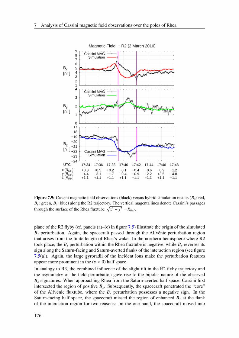
7 Analysis of Cassini magnetic field observations over the poles of Rhea
1 2 3 4 5 6 7 8 9
17:34 17:36 17:38 17:40 17:42 17:44 17:46 17:48
Magnetic Field − R2 (2 March 2010)
Bx [nT]
Cassini MAGSimulation
0
1
2
3
4
17:34 17:36 17:38 17:40 17:42 17:44 17:46 17:48
By [nT]
Cassini MAGSimulation
−24−23−22−21−20−19−18−17
17:34 17:36 17:38 17:40 17:42 17:44 17:46 17:48UTCx [RRH]y [RRH]z [RRH]
+0.8−4.4+1.1
+0.5−3.1+1.1
+0.2−1.7+1.1
−0.1−0.4+1.1
−0.4+0.9+1.1
−0.6+2.2+1.1
−0.9+3.5+1.1
−1.2+4.8+1.1
Bz [nT] Cassini MAG
Simulation
Figure 7.9: Cassini magnetic field observations (black) versus hybrid simulation results (Bx: red,By: green, Bz: blue) along the R2 trajectory. The vertical magenta lines denote Cassini’s passagesthrough the surface of the Rhea fluxtube
√x2 + y2 = RRH .
plane of the R2 flyby (cf. panels (a)–(c) in figure 7.5) illustrate the origin of the simulatedBx perturbation. Again, the spacecraft passed through the Alfvénic perturbation regionthat arises from the finite length of Rhea’s wake. In the northern hemisphere where R2took place, the Bx perturbation within the Rhea fluxtube is negative, while Bx reverses itssign along the Saturn-facing and Saturn-averted flanks of the interaction region (see figure7.5(a)). Again, the large gyroradii of the incident ions make the perturbation featuresappear more prominent in the (y < 0) half space.In analogy to R3, the combined influence of the slight tilt in the R2 flyby trajectory andthe asymmetry of the field perturbation gave rise to the bipolar nature of the observedBx signatures. When approaching Rhea from the Saturn-averted half space, Cassini firstintersected the region of positive Bx. Subsequently, the spacecraft penetrated the “core”of the Alfvénic fluxtube, where the Bx perturbation possesses a negative sign. In theSaturn-facing half space, the spacecraft missed the region of enhanced Bx at the flankof the interaction region for two reasons: on the one hand, the spacecraft moved into
176
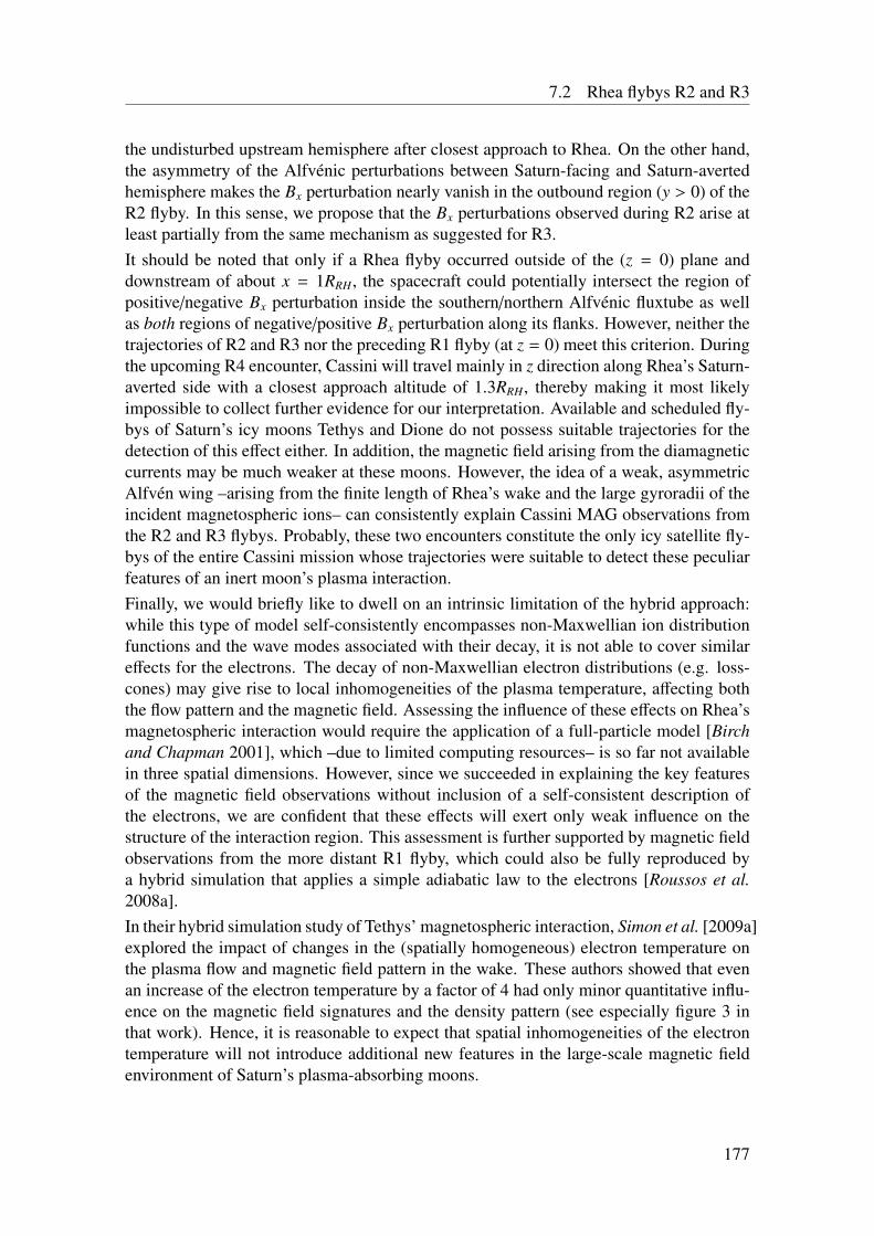
7.2 Rhea flybys R2 and R3
the undisturbed upstream hemisphere after closest approach to Rhea. On the other hand,the asymmetry of the Alfvénic perturbations between Saturn-facing and Saturn-avertedhemisphere makes the Bx perturbation nearly vanish in the outbound region (y > 0) of theR2 flyby. In this sense, we propose that the Bx perturbations observed during R2 arise atleast partially from the same mechanism as suggested for R3.It should be noted that only if a Rhea flyby occurred outside of the (z = 0) plane anddownstream of about x = 1RRH, the spacecraft could potentially intersect the region ofpositive/negative Bx perturbation inside the southern/northern Alfvénic fluxtube as wellas both regions of negative/positive Bx perturbation along its flanks. However, neither thetrajectories of R2 and R3 nor the preceding R1 flyby (at z = 0) meet this criterion. Duringthe upcoming R4 encounter, Cassini will travel mainly in z direction along Rhea’s Saturn-averted side with a closest approach altitude of 1.3RRH, thereby making it most likelyimpossible to collect further evidence for our interpretation. Available and scheduled fly-bys of Saturn’s icy moons Tethys and Dione do not possess suitable trajectories for thedetection of this effect either. In addition, the magnetic field arising from the diamagneticcurrents may be much weaker at these moons. However, the idea of a weak, asymmetricAlfvén wing –arising from the finite length of Rhea’s wake and the large gyroradii of theincident magnetospheric ions– can consistently explain Cassini MAG observations fromthe R2 and R3 flybys. Probably, these two encounters constitute the only icy satellite fly-bys of the entire Cassini mission whose trajectories were suitable to detect these peculiarfeatures of an inert moon’s plasma interaction.Finally, we would briefly like to dwell on an intrinsic limitation of the hybrid approach:while this type of model self-consistently encompasses non-Maxwellian ion distributionfunctions and the wave modes associated with their decay, it is not able to cover similareffects for the electrons. The decay of non-Maxwellian electron distributions (e.g. loss-cones) may give rise to local inhomogeneities of the plasma temperature, affecting boththe flow pattern and the magnetic field. Assessing the influence of these effects on Rhea’smagnetospheric interaction would require the application of a full-particle model [Birchand Chapman 2001], which –due to limited computing resources– is so far not availablein three spatial dimensions. However, since we succeeded in explaining the key featuresof the magnetic field observations without inclusion of a self-consistent description ofthe electrons, we are confident that these effects will exert only weak influence on thestructure of the interaction region. This assessment is further supported by magnetic fieldobservations from the more distant R1 flyby, which could also be fully reproduced bya hybrid simulation that applies a simple adiabatic law to the electrons [Roussos et al.2008a].In their hybrid simulation study of Tethys’ magnetospheric interaction, Simon et al. [2009a]explored the impact of changes in the (spatially homogeneous) electron temperature onthe plasma flow and magnetic field pattern in the wake. These authors showed that evenan increase of the electron temperature by a factor of 4 had only minor quantitative influ-ence on the magnetic field signatures and the density pattern (see especially figure 3 inthat work). Hence, it is reasonable to expect that spatial inhomogeneities of the electrontemperature will not introduce additional new features in the large-scale magnetic fieldenvironment of Saturn’s plasma-absorbing moons.
177

8 Summary and Outlook
In this thesis, the plasma environments of the Saturnian moons Enceladus and Rhea –which are located deeply within Saturn’s magnetosphere – have been studied. Both icymoons have in common that their surfaces are completely covered with water ice. Thesatellites’ interactions with Saturn’s magnetospheric plasma, however, represent two com-pletely different types of interaction scenarios. On the one hand, the extended plume ofwater vapor and dust originating from Enceladus’ south polar region gives rise to a sub-alfvénic ionosphere-type interaction: the neutral plume is ionized by means of chargeexchange, photoionization and electron impacts. The subsequent pick-up of the ions andelectrons and the associated currents generate a non-linear system of standing Alfvénwaves, the Alfvén wing. On the other hand, particle absorption at the surface of Saturn’ssecond-largest moon Rhea corresponds to an inert-moon type of interaction, similar tothat of the Earth’s moon.Analytical modeling and numerical simulations by means of the hybrid code A.I.K.E.F.(Adaptive Ion-Kinetic Electron-Fluid) have been used to analyze the plasma structures inthe vicinity of the icy moons. It turned out that A.I.K.E.F. is particularly suitable to studythese plasma interactions, since the charged dust in Enceladus’ plume could be easilyincluded in the hybrid model and the treatment of the inner boundary at the surfaces ofthe satellites allows a correct description of processes associated with plasma absorptionby the solid body of Rhea.The simulation results are compared with various measurements from the Cassini space-craft. In particular the magnetic field measurements obtained during the 20 Enceladusand five Rhea flybys that were available at the time of this thesis were set into a three-dimensional context. Surprisingly, it turned out that both moons have in common thatthey generate an Alfvén wing that is unique, either in terms of its properties or with re-spect to its generation. The study of the underlying processes helped to interpret Cassinidata and substantially enlarged our understanding of the respective plasma interaction.The particular results of this thesis are summarized in the following.
8.1 Enceladus
In part one of the study of Enceladus’ plasma interaction (chapter 5), the influence of elec-tron absorption by negatively charged dust on the structure of Enceladus’ Alfvén wingswas investigated. For a first basic analysis, charged dust was included in the analyticalmodeling of the Alfvén wing as well as in simulations of a corresponding test scenario.The major findings were:
179
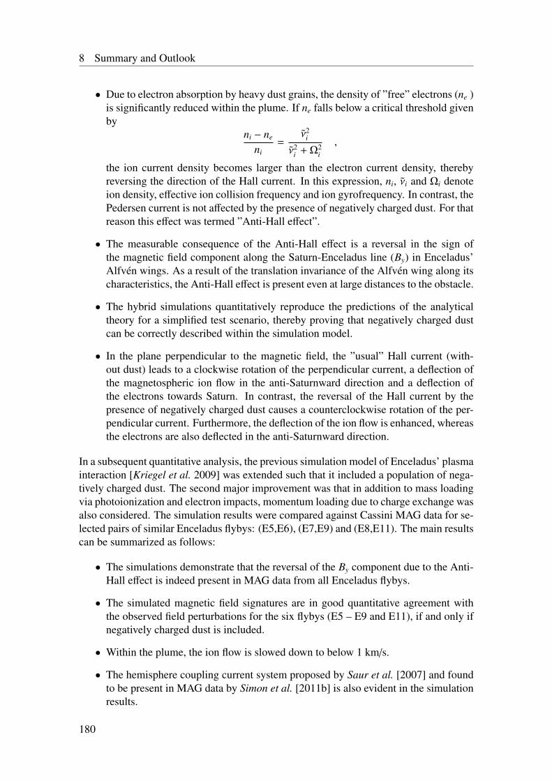
8 Summary and Outlook
• Due to electron absorption by heavy dust grains, the density of ”free” electrons (ne )is significantly reduced within the plume. If ne falls below a critical threshold givenby
ni − ne
ni=
ν2i
ν2i + Ω2
i
,
the ion current density becomes larger than the electron current density, therebyreversing the direction of the Hall current. In this expression, ni, νi and Ωi denoteion density, effective ion collision frequency and ion gyrofrequency. In contrast, thePedersen current is not affected by the presence of negatively charged dust. For thatreason this effect was termed ”Anti-Hall effect”.
• The measurable consequence of the Anti-Hall effect is a reversal in the sign ofthe magnetic field component along the Saturn-Enceladus line (By) in Enceladus’Alfvén wings. As a result of the translation invariance of the Alfvén wing along itscharacteristics, the Anti-Hall effect is present even at large distances to the obstacle.
• The hybrid simulations quantitatively reproduce the predictions of the analyticaltheory for a simplified test scenario, thereby proving that negatively charged dustcan be correctly described within the simulation model.
• In the plane perpendicular to the magnetic field, the ”usual” Hall current (with-out dust) leads to a clockwise rotation of the perpendicular current, a deflection ofthe magnetospheric ion flow in the anti-Saturnward direction and a deflection ofthe electrons towards Saturn. In contrast, the reversal of the Hall current by thepresence of negatively charged dust causes a counterclockwise rotation of the per-pendicular current. Furthermore, the deflection of the ion flow is enhanced, whereasthe electrons are also deflected in the anti-Saturnward direction.
In a subsequent quantitative analysis, the previous simulation model of Enceladus’ plasmainteraction [Kriegel et al. 2009] was extended such that it included a population of nega-tively charged dust. The second major improvement was that in addition to mass loadingvia photoionization and electron impacts, momentum loading due to charge exchange wasalso considered. The simulation results were compared against Cassini MAG data for se-lected pairs of similar Enceladus flybys: (E5,E6), (E7,E9) and (E8,E11). The main resultscan be summarized as follows:
• The simulations demonstrate that the reversal of the By component due to the Anti-Hall effect is indeed present in MAG data from all Enceladus flybys.
• The simulated magnetic field signatures are in good quantitative agreement withthe observed field perturbations for the six flybys (E5 – E9 and E11), if and only ifnegatively charged dust is included.
• Within the plume, the ion flow is slowed down to below 1 km/s.
• The hemisphere coupling current system proposed by Saur et al. [2007] and foundto be present in MAG data by Simon et al. [2011b] is also evident in the simulationresults.
180
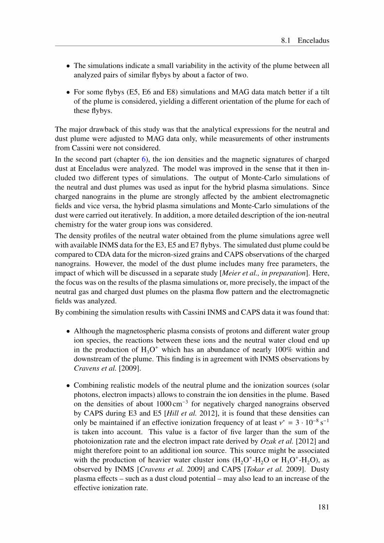
8.1 Enceladus
• The simulations indicate a small variability in the activity of the plume between allanalyzed pairs of similar flybys by about a factor of two.
• For some flybys (E5, E6 and E8) simulations and MAG data match better if a tiltof the plume is considered, yielding a different orientation of the plume for each ofthese flybys.
The major drawback of this study was that the analytical expressions for the neutral anddust plume were adjusted to MAG data only, while measurements of other instrumentsfrom Cassini were not considered.In the second part (chapter 6), the ion densities and the magnetic signatures of chargeddust at Enceladus were analyzed. The model was improved in the sense that it then in-cluded two different types of simulations. The output of Monte-Carlo simulations ofthe neutral and dust plumes was used as input for the hybrid plasma simulations. Sincecharged nanograins in the plume are strongly affected by the ambient electromagneticfields and vice versa, the hybrid plasma simulations and Monte-Carlo simulations of thedust were carried out iteratively. In addition, a more detailed description of the ion-neutralchemistry for the water group ions was considered.The density profiles of the neutral water obtained from the plume simulations agree wellwith available INMS data for the E3, E5 and E7 flybys. The simulated dust plume could becompared to CDA data for the micron-sized grains and CAPS observations of the chargednanograins. However, the model of the dust plume includes many free parameters, theimpact of which will be discussed in a separate study [Meier et al., in preparation]. Here,the focus was on the results of the plasma simulations or, more precisely, the impact of theneutral gas and charged dust plumes on the plasma flow pattern and the electromagneticfields was analyzed.By combining the simulation results with Cassini INMS and CAPS data it was found that:
• Although the magnetospheric plasma consists of protons and different water groupion species, the reactions between these ions and the neutral water cloud end upin the production of H3O+ which has an abundance of nearly 100% within anddownstream of the plume. This finding is in agreement with INMS observations byCravens et al. [2009].
• Combining realistic models of the neutral plume and the ionization sources (solarphotons, electron impacts) allows to constrain the ion densities in the plume. Basedon the densities of about 1000 cm−3 for negatively charged nanograins observedby CAPS during E3 and E5 [Hill et al. 2012], it is found that these densities canonly be maintained if an effective ionization frequency of at least ν∗ = 3 · 10−8 s−1
is taken into account. This value is a factor of five larger than the sum of thephotoionization rate and the electron impact rate derived by Ozak et al. [2012] andmight therefore point to an additional ion source. This source might be associatedwith the production of heavier water cluster ions (H2O+-H2O or H3O+-H2O), asobserved by INMS [Cravens et al. 2009] and CAPS [Tokar et al. 2009]. Dustyplasma effects – such as a dust cloud potential – may also lead to an increase of theeffective ionization rate.
181
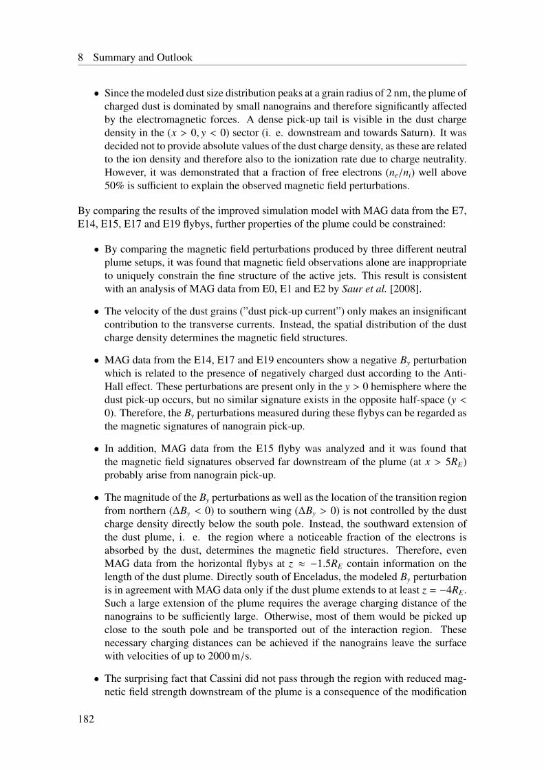
8 Summary and Outlook
• Since the modeled dust size distribution peaks at a grain radius of 2 nm, the plume ofcharged dust is dominated by small nanograins and therefore significantly affectedby the electromagnetic forces. A dense pick-up tail is visible in the dust chargedensity in the (x > 0, y < 0) sector (i. e. downstream and towards Saturn). It wasdecided not to provide absolute values of the dust charge density, as these are relatedto the ion density and therefore also to the ionization rate due to charge neutrality.However, it was demonstrated that a fraction of free electrons (ne/ni) well above50% is sufficient to explain the observed magnetic field perturbations.
By comparing the results of the improved simulation model with MAG data from the E7,E14, E15, E17 and E19 flybys, further properties of the plume could be constrained:
• By comparing the magnetic field perturbations produced by three different neutralplume setups, it was found that magnetic field observations alone are inappropriateto uniquely constrain the fine structure of the active jets. This result is consistentwith an analysis of MAG data from E0, E1 and E2 by Saur et al. [2008].
• The velocity of the dust grains (”dust pick-up current”) only makes an insignificantcontribution to the transverse currents. Instead, the spatial distribution of the dustcharge density determines the magnetic field structures.
• MAG data from the E14, E17 and E19 encounters show a negative By perturbationwhich is related to the presence of negatively charged dust according to the Anti-Hall effect. These perturbations are present only in the y > 0 hemisphere where thedust pick-up occurs, but no similar signature exists in the opposite half-space (y <0). Therefore, the By perturbations measured during these flybys can be regarded asthe magnetic signatures of nanograin pick-up.
• In addition, MAG data from the E15 flyby was analyzed and it was found thatthe magnetic field signatures observed far downstream of the plume (at x > 5RE)probably arise from nanograin pick-up.
• The magnitude of the By perturbations as well as the location of the transition regionfrom northern (∆By < 0) to southern wing (∆By > 0) is not controlled by the dustcharge density directly below the south pole. Instead, the southward extension ofthe dust plume, i. e. the region where a noticeable fraction of the electrons isabsorbed by the dust, determines the magnetic field structures. Therefore, evenMAG data from the horizontal flybys at z ≈ −1.5RE contain information on thelength of the dust plume. Directly south of Enceladus, the modeled By perturbationis in agreement with MAG data only if the dust plume extends to at least z = −4RE.Such a large extension of the plume requires the average charging distance of thenanograins to be sufficiently large. Otherwise, most of them would be picked upclose to the south pole and be transported out of the interaction region. Thesenecessary charging distances can be achieved if the nanograins leave the surfacewith velocities of up to 2000 m/s.
• The surprising fact that Cassini did not pass through the region with reduced mag-netic field strength downstream of the plume is a consequence of the modification
182
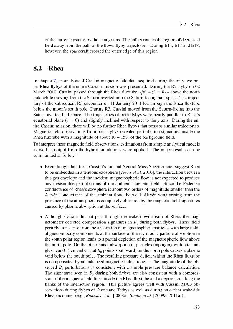
8.2 Rhea
of the current systems by the nanograins. This effect rotates the region of decreasedfield away from the path of the flown flyby trajectories. During E14, E17 and E18,however, the spacecraft crossed the outer edge of this region.
8.2 Rhea
In chapter 7, an analysis of Cassini magnetic field data acquired during the only two po-lar Rhea flybys of the entire Cassini mission was presented. During the R2 flyby on 02March 2010, Cassini passed through the Rhea fluxtube
√y2 + z2 = RRH above the north
pole while moving from the Saturn-averted into the Saturn-facing half space. The trajec-tory of the subsequent R3 encounter on 11 January 2011 led through the Rhea fluxtubebelow the moon’s south pole. During R3, Cassini moved from the Saturn-facing into theSaturn-averted half space. The trajectories of both flybys were nearly parallel to Rhea’sequatorial plane (z = 0) and slightly inclined with respect to the y axis. During the en-tire Cassini mission, there will be no further Rhea flybys that possess similar trajectories.Magnetic field observations from both flybys revealed perturbation signatures inside theRhea fluxtube with a magnitude of about 10 − 15% of the background field.To interpret these magnetic field observations, estimations from simple analytical modelsas well as output from the hybrid simulations were applied. The major results can besummarized as follows:
• Even though data from Cassini’s Ion and Neutral Mass Spectrometer suggest Rheato be embedded in a tenuous exosphere [Teolis et al. 2010], the interaction betweenthis gas envelope and the incident magnetospheric flow is not expected to produceany measurable perturbations of the ambient magnetic field. Since the Pedersenconductance of Rhea’s exosphere is about two orders of magnitude smaller than theAlfvén conductance of the ambient flow, the weak Alfvén wing arising from thepresence of the atmosphere is completely obscured by the magnetic field signaturescaused by plasma absorption at the surface.
• Although Cassini did not pass through the wake downstream of Rhea, the mag-netometer detected compression signatures in Bz during both flybys. These fieldperturbations arise from the absorption of magnetospheric particles with large field-aligned velocity components at the surface of the icy moon: particle absorption inthe south polar region leads to a partial depletion of the magnetospheric flow abovethe north pole. On the other hand, absorption of particles impinging with pitch an-gles near 0 (remember that B0 points southward) on the north pole causes a plasmavoid below the south pole. The resulting pressure deficit within the Rhea fluxtubeis compensated by an enhanced magnetic field strength. The magnitude of the ob-served Bz perturbations is consistent with a simple pressure balance calculation.The signatures seen in By during both flybys are also consistent with a compres-sion of the magnetic field lines inside the Rhea fluxtube and a depression along theflanks of the interaction region. This picture agrees well with Cassini MAG ob-servations during flybys of Dione and Tethys as well as during an earlier wakesideRhea encounter (e.g., Roussos et al. [2008a], Simon et al. [2009a, 2011a]).
183
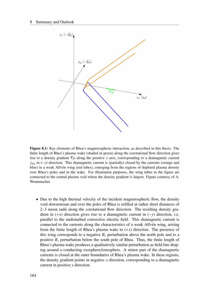
8 Summary and Outlook
Figure 8.1: Key elements of Rhea’s magnetospheric interaction, as described in this thesis. Thefinite length of Rhea’s plasma wake (shaded in green) along the corotational flow direction givesrise to a density gradient ∇p along the positive x axis, corresponding to a diamagnetic currentjdia in (−y) direction. This diamagnetic current is (partially) closed by the currents (orange andblue) in a weak Alfvén wing (red tubes), emerging from the regions of depleted plasma densityover Rhea’s poles and in the wake. For illustration purposes, the wing tubes in the figure areconnected to the central plasma void where the density gradient is largest. Figure courtesy of A.Wennmacher.
• Due to the high thermal velocity of the incident magnetospheric flow, the densityvoid downstream and over the poles of Rhea is refilled at rather short distances of2–3 moon radii along the corotational flow direction. The resulting density gra-dient in (+x) direction gives rise to a diamagnetic current in (−y) direction, i.e.parallel to the undisturbed convective electric field. This diamagnetic current isconnected to the currents along the characteristics of a weak Alfvén wing, arisingfrom the finite length of Rhea’s plasma wake in (+x) direction. The presence ofthis wing corresponds to a negative Bx perturbation above the north pole and to apositive Bx perturbation below the south pole of Rhea. Thus, the finite length ofRhea’s plasma wake produces a qualitatively similar perturbation as field line drap-ing around a conducting exosphere/ionosphere. A minor part of the diamagneticcurrents is closed at the outer boundaries of Rhea’s plasma wake. In these regions,the density gradient points in negative x direction, corresponding to a diamagneticcurrent in positive y direction.
184
8.3 Outlook
• The intensity of the flow-aligned magnetic field perturbations is not only propor-tional to the pressure gradient in the wake, but it also decreases with increasingstrength of the ambient magnetospheric field. The plasma environment of Rhea,featuring a rather large beta value of βi + βe ≈ 1, is therefore particularly suitablefor observing these signatures. Even if flybys of Tethys or Dione possessed suit-able trajectories to detect this effect, the stronger background magnetospheric fieldnear the orbits of these satellites (βi + βe 1) would most probably prevent theformation of any measurable flow-aligned field perturbations.
• The ion gyroradii in the incident magnetospheric flow are comparable to the size ofthe Rhea, thereby making plasma absorption at the surface of the moon asymmetricwith respect to the direction of the convective electric field. This effect also causesan asymmetry in the structure of the Alfvén wing: in the Saturn-averted hemispherewhere the convective electric field points away from Rhea, the magnetic field per-turbations are more intense than in the Saturn-facing hemisphere. Magnetic fieldobservations from both R2 and R3 are qualitatively consistent with the presenceof this asymmetric Alfvén wing structure, generated by the finite length of Rhea’swake. Additional close flybys of Rhea would be required to further strengthen thisprediction of the hybrid simulation.
Figure 8.1 summarizes our current understanding of Rhea’s magnetospheric interaction.
8.3 Outlook
Although excellent agreement between the modeled magnetic field signatures and CassiniMAG data was achieved for a number of flybys of Enceladus and Rhea, there are stillvarious features in the data that are not reproduced by the simulations. This points to astill oversimplified model and/or additional processes which are not yet considered.In appendix B, those Enceladus flybys are discussed, for which the results are (partially)only in rough agreement with MAG data. A few test runs were carried out to analyzethe origin of the most apparent discrepancies. From these simulations as well as from theresults presented in chapters 5 and 6, it was learned that the following issues should beaddressed in future work:
• Even though the simulations discussed in chapter 6 are based on a neutral plumein agreement with INMS data, MAG data from the steep flybys E3 – E6 could bereproduced only for a neutral plume which is almost as narrow as the one appliedin chapter 5. Up to now, no simulation setup could be found which simultaneouslyexplains MAG and INMS data for these flybys.
• The Bz perturbations measured above Enceladus’ north pole during E12 and E13as well as during the far downstream encounter E15 feature a puzzling increase ofa few nT around closest approach. The magnitude of these perturbations wouldbe roughly consistent with an enhanced magnetic field compensating for a lackof plasma pressure similar to Rhea’s wake. However, at Enceladus, the plasma isdeflected around the Alfvén wing before it impinges on the surface. In particular
185
8 Summary and Outlook
for E15, the simulations would be more likely consistent with an increase of plasmapressure due to the increased ion density in the pick-up tail. It is therefore not clearwhy a plasma density cavity should be present in these regions.
• The fact that – at least for some of the flybys like E7 – the simplified analyticalexpression for the dust charge density yields better agreement with MAG data thanthe dust plume resulting from the Monte-Carlo simulations shows that Enceladus’cloud of charged dust is still considerably different from that generated by the sim-ulations. In particular at the Saturn-averted side of the plume (outbound of E7 andE9, inbound of E14 and E17 – E19), the simulated By perturbations are clearlyweaker than the measured perturbations. This may indicate that the Anti-Hall effectneeds to be stronger in this region, and consequently the dust charge density needsto be higher in the direction opposite to the dust pick-up. The reasons for the dif-ferences to our modeling efforts could be manifold: the real dust size distributioncould favor larger grains which would imply less pick-up; the ionization frequency(and the resulting plasma densities) might be larger or smaller which would alterthe grain charging; the dust jets might be more collimated than assumed or some ofthem might be oriented away from Saturn.
• MAG data from the horizontal flybys discussed in chapter 6 exhibit magnetic fielddiscontinuities exactly at the Enceladus flux tube which are likely associated withthe hemisphere coupling current system proposed by Saur et al. [2007]. However,these discontinuities seem to be present only in the Saturn-facing hemisphere. Thismay be linked to the asymmetric distribution of auroral hiss (strong whistler modeemissions) which are generated by field-aligned currents [Leisner et al. 2013]. Thecause of these asymmetries should be investigated.
• The high densities of negatively charged dust may also lead to fundamental changesin the nature of the plasma, i.e. dusty plasma effects like the dust cloud potentialmay play a key role in understanding the details of the physics within the plume.Incorporating the dust cloud potential may also lead to a self-consistent model ofthe ion source ν∗.
• The future flybys E20 and E22 are going to be located 10RE above and 20RE belowEnceladus’ poles, respectively. Thus, these flybys are going to provide the uniqueopportunity to study the northern and southern Alfvén wing in the far field, therebyallowing to further constrain the extent of the plume in the plane perpendicular tothe magnetic field.
• Unfortunately, some results also reveal numerical artifacts. For instance, a wavestructure with a wave length corresponding to the mesh can be clearly seen in fig-ure 6.12. Furthermore, the offset between simulated Bz component and MAG datainbound of the encounters E14, E17 and E19 (cf. figures 6.10 and 6.13) is associ-ated with an artificial extent of the magnetic field pile-up region. However, it shouldbe pointed out that it has been very thoroughly checked that these artifacts do notaffect the aspects of the simulated magnetic field structures that are discussed inthis thesis, nor do they alter any of the conclusions. Nevertheless, these numericaleffects should be eliminated in future work.
186
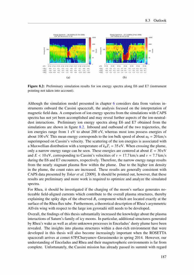
8.3 Outlook
Energy Spectrum − E6 (91EN) (31 Oct 2008) C/A: 197 km at UTC 17:15
x [RE]y [RE]z [RE]
+9.0−0.8+13.6
+7.1−0.6+9.9
+5.1−0.5+6.2
+3.2−0.2+2.4
+1.2−0.0−1.3
−0.8+0.2−5.0
−2.7+0.4−8.8
−4.7+0.7−12.5
−6.6+1.0−16.2
−8.6+1.2−19.9
UTC 17:11 17:12 17:13 17:14 17:15 17:16 17:17 17:18 17:19 17:20 1
100
Ene
rgy
[eV
]
1
10
100
1000
10000
Cou
nts
(a)
Energy Spectrum − E7 (120EN) (2 Nov 2009) C/A: 103 km at UTC 07:42
x [RE]y [RE]z [RE]
−3.5+8.5−1.5
−2.8+6.7−1.5
−2.1+5.1−1.5
−1.4+3.4−1.4
−0.7+1.6−1.4
0.00.0−1.4
+0.7−1.7−1.3
+1.4−3.5−1.3
+2.0−5.2−1.3
+2.7−6.9−1.3
+3.3−8.7−1.2
UTC 07:39 07:40 07:41 07:42 07:43 07:44 07:45 1
100
Ene
rgy
[eV
]
1
10
100
1000
10000
Cou
nts
(b)
Figure 8.2: Preliminary simulation results for ion energy spectra along E6 and E7 (instrumentpointing not taken into account).
Although the simulation model presented in chapter 6 considers data from various in-struments onboard the Cassini spacecraft, the analysis focused on the interpretation ofmagnetic field data. A comparison of ion energy spectra from the simulations with CAPSspectra has not yet been accomplished and may reveal further aspects of the ion-neutral-dust interactions. Preliminary ion energy spectra along E6 and E7 obtained from thesimulations are shown in figure 8.2. Inbound and outbound of the two trajectories, theion energies range from 1 eV to about 200 eV, whereas most ions possess energies ofabout 100 eV. This mean energy corresponds to the ion bulk speed of about u0 = 20 km/ssuperimposed on Cassini’s velocity. The scattering of the ion energies is associated witha Maxwellian distribution with a temperature of kBTi = 35 eV. When crossing the plume,only a narrow energy range can be seen. These energies are centered at about E = 30 eVand E < 10 eV, corresponding to Cassini’s velocities of v = 17.7 km/s and v = 7.7 km/sduring the E6 and E7 encounters, respectively. Therefore, the narrow energy range resultsfrom the nearly stagnant plasma flow within the plume. Due to the higher ion densityin the plume, the count rates are increased. These results are generally consistent withCAPS data presented by Tokar et al. [2009]. It should be pointed out, however, that theseresults are preliminary and more work is required to optimize and analyze the simulatedspectra.For Rhea, it should be investigated if the charging of the moon’s surface generates no-ticeable field-aligned currents which contribute to the overall plasma structures, therebyexplaining the spiky dips of the observed Bx component which are located exactly at thesurface of the Rhea flux tube. Furthermore, a theoretical description of Rhea’s asymmetricAlfvén wing with respect to the large ion gyroradii still needs to be developed.Overall, the findings of this thesis substantially increased the knowledge about the plasmainteractions of Saturn’s family of icy moons. In particular, additional structures generatedby Rhea’s wake as well as afore unknown processes in Enceladus’ dusty plume have beenrevealed. The insights into plasma structures within a dust-rich environment that weredeveloped in this thesis will also become increasingly important when the ROSETTAspacecraft arrives at comet 67P/Churyumov-Gerasimenko in spring 2014. However, ourunderstanding of Enceladus and Rhea and their magnetospheric environments is far fromcomplete. Unfortunately, the Cassini mission has already passed its summit with regard
187

8 Summary and Outlook
to flybys of the icy moons. The spacecraft is going to perform only three additional Ence-ladus flybys and no further flyby of Rhea that could provide new in situ data. The huge setof data already collected by Cassini will, however, still allow to make new and spectaculardiscoveries within the next years or even decades, before we visit these fascinating moonsagain.
188
A Reaction and Ionization Rates
The ion-neutral interactions considered in our model are provided in table 6.2 of the mainpaper. There, the reaction rates kα,β(u0) were listed at the upstream speed u0 for refer-ence. In this appendix, we provide the expressions for the velocity-dependent reactionrates kα,β(vrel) which are applied in our model. Two different interaction mechanisms areincluded: elastic ion-neutral collisions and charge exchange (see section 4.3).The elastic ion-neutral collisions are approximated by induced dipole interactions (ID),i.e. the approaching ion leads to a polarization of the neutral [Schunk and Nagy 2009]. Insuch a case, the interaction potential V is given by
V = −1
4πε0
γne2
r, (A.1)
where γn denotes the polarizability of the neutral and r the distance between the ion andthe neutral. Collisions associated with this interaction potential are also referred to as”Maxwell molecule collisions”. The corresponding the cross section σID
α (vrel) in units ofcm2 is (see e. g. Schunk and Nagy [2009], eq. (4.88))
σIDα (vrel) = 2.21π
√γnα f ite2
µαv2rel
, (A.2)
where vrel is the relative velocity between the reactants in cm/s, γn = 1.48·10−24 cm3 is thepolarizability of H2O and µα and e = 4.8 · 10−10 esu denote reduced mass and elementarycharge, respectively. CGS units are used in equation (A.2). α f it is a fudge parameterto match the laboratory measured rates (e. g. http://www.udfa.net UMIST database forAstrochemistry). Physically, it accounts for the permanent electric dipole of the watermolecules. The values for α f it are listed in table A.1. Since σID
α ∝ v−1rel, the corresponding
reaction rate kIDα,β = vrelσ
IDα is independent of the velocity.
The resonant charge exchange cross section σCXα (vrel) (in cm2) can be expressed as (see
e.g., Schunk and Nagy [2009], eq. (4.148))
σCXα (vrel) =
(Aα − Bα log10 (εα)
)2−Cα log10(vrel) , (A.3)
where εα = µαv2rel/2 (in eV) denotes the relative kinetic energy of the colliding particles.
The last term on the right hand side of equation (A.3) has been added to match the labora-tory measured rates. Here, the velocity vrel has to be inserted in units of cm/s. The valuesof the constants Aα, Bα and Cα are listed in table A.1. If different energy states of the ionsneed to be considered, the expression becomes more complex [Nakai et al. 1987]:
189
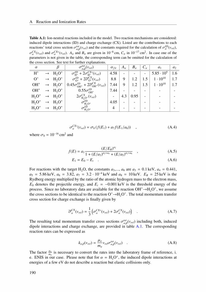
A Reaction and Ionization Rates
Table A.1: Ion-neutral reactions included in the model. Two reaction mechanisms are considered:induced dipole interactions (ID) and charge exchange (CX). Listed are the contributions to eachreactions’ total cross section σtot
α,β(vrel) and the constants required for the calculation of σIDα (vrel),
σCXα (vrel) and σCX∗
α (vrel). Aα and Bα are given in 10−8 cm, Cα in 10−17 cm2. In case one of theparameters is not given in the table, the corresponding term can be omitted for the calculation ofthe cross section. See text for further explanations.
α β σtotα,β(vrel) α f it Aα Bα Cα a1 a2
H+→ H2O+ σID
H+ + 2σCX∗H+ (vrel) 4.58 - - - 5.85 · 105 1.6
O+→ H2O+ σID
O+ + 2σCXO+ (vrel) 8.8 9 1.2 1.5 1 · 1010 1.7
OH+→ H2O+ 0.45σID
OH+ + 2σCXOH+(vrel) 7.44 9 1.2 1.5 1 · 1010 1.7
OH+→ H3O+ 0.55σID
OH+ 7.44 - - - - -H2O+
→ H2O+ 2σCXH2O+(vrel) - 4.3 0.95 - - -
H2O+→ H3O+ σID
H2O+ 4.05 - - - - -H3O+
→ H3O+ σIDH3O+ 4 - - - - -
σCX∗α (vrel) = σ0 ( f (E1) + a7 f (E1/a8)) , (A.4)
where σ0 = 10−16 cm2 and
f (E) = a1(E/ER)a2
1 + (E/a3)a2+a4 + (E/a5)a2+a6, (A.5)
E1 = E0 − Et . (A.6)
For reactions with the target H2O, the constants a3,..., a8 are a3 = 0.1 keV, a4 = 0.441,a5 = 5.86 keV, a6 = 3.82, a7 = 3.2 · 10−4 keV and a8 = 10 keV. ER = 25 keV is theRydberg energy multiplied by the ratio of the atomic hydrogen mass to the electron mass,E0 denotes the projectile energy, and Et = −0.001 keV is the threshold energy of theprocess. Since no laboratory data are available for the reaction OH+
→H2O+, we assumethe cross sections to be identical to the reaction O+
→H2O+. The total momentum transfercross section for charge exchange is finally given by
σCXα (vrel) =
13
(σCX∗α (vrel) + 2σCX
α (vrel))
. (A.7)
The resulting total momentum transfer cross sections σtotα,β(vrel) including both, induced
dipole interactions and charge exchange, are provided in table A.1. The correspondingreaction rates can be expressed as
kα,β(vrel) =µαmα
vrelσtotα,β(vrel) . (A.8)
The factor µαmα
is necessary to convert the rates into the laboratory frame of reference, i.e. ENIS in our case. Please note that for α = H3O+, the induced dipole interactions atenergies of a few eV do not describe a reaction but elastic collisions only.
190
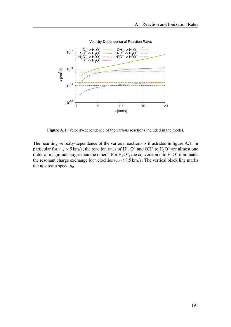
A Reaction and Ionization Rates
10-10
10-9
10-8
10-7
0 5 10 15 20
k [c
m3 /s
]
ui [km/s]
Velocity-Dependence of Reaction Rates
O+ -> H2O+
OH+ -> H2O+
H2O+ -> H2O+
H+ -> H2O+
OH+ -> H3O+
H2O+ -> H3O+
H3O+ -> H3O+
Figure A.1: Velocity-dependence of the various reactions included in the model.
The resulting velocity-dependence of the various reactions is illustrated in figure A.1. Inparticular for vrel > 5 km/s, the reaction rates of H+, O+ and OH+ to H2O+ are almost oneorder of magnitude larger than the others. For H2O+, the conversion into H3O+ dominatesthe resonant charge exchange for velocities vrel < 8.5 km/s. The vertical black line marksthe upstream speed u0.
191

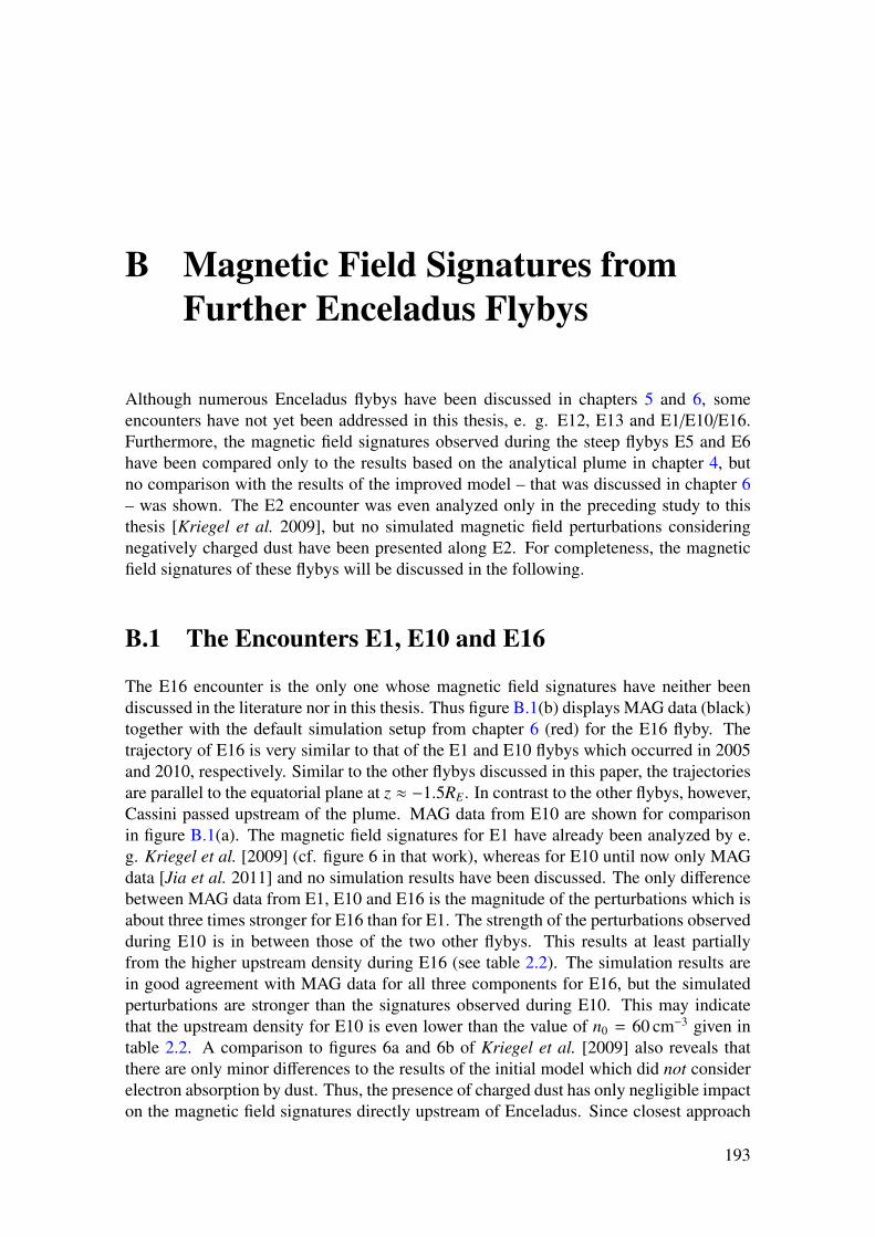
B Magnetic Field Signatures fromFurther Enceladus Flybys
Although numerous Enceladus flybys have been discussed in chapters 5 and 6, someencounters have not yet been addressed in this thesis, e. g. E12, E13 and E1/E10/E16.Furthermore, the magnetic field signatures observed during the steep flybys E5 and E6have been compared only to the results based on the analytical plume in chapter 4, butno comparison with the results of the improved model – that was discussed in chapter 6– was shown. The E2 encounter was even analyzed only in the preceding study to thisthesis [Kriegel et al. 2009], but no simulated magnetic field perturbations consideringnegatively charged dust have been presented along E2. For completeness, the magneticfield signatures of these flybys will be discussed in the following.
B.1 The Encounters E1, E10 and E16
The E16 encounter is the only one whose magnetic field signatures have neither beendiscussed in the literature nor in this thesis. Thus figure B.1(b) displays MAG data (black)together with the default simulation setup from chapter 6 (red) for the E16 flyby. Thetrajectory of E16 is very similar to that of the E1 and E10 flybys which occurred in 2005and 2010, respectively. Similar to the other flybys discussed in this paper, the trajectoriesare parallel to the equatorial plane at z ≈ −1.5RE. In contrast to the other flybys, however,Cassini passed upstream of the plume. MAG data from E10 are shown for comparisonin figure B.1(a). The magnetic field signatures for E1 have already been analyzed by e.g. Kriegel et al. [2009] (cf. figure 6 in that work), whereas for E10 until now only MAGdata [Jia et al. 2011] and no simulation results have been discussed. The only differencebetween MAG data from E1, E10 and E16 is the magnitude of the perturbations which isabout three times stronger for E16 than for E1. The strength of the perturbations observedduring E10 is in between those of the two other flybys. This results at least partiallyfrom the higher upstream density during E16 (see table 2.2). The simulation results arein good agreement with MAG data for all three components for E16, but the simulatedperturbations are stronger than the signatures observed during E10. This may indicatethat the upstream density for E10 is even lower than the value of n0 = 60 cm−3 given intable 2.2. A comparison to figures 6a and 6b of Kriegel et al. [2009] also reveals thatthere are only minor differences to the results of the initial model which did not considerelectron absorption by dust. Thus, the presence of charged dust has only negligible impacton the magnetic field signatures directly upstream of Enceladus. Since closest approach
193
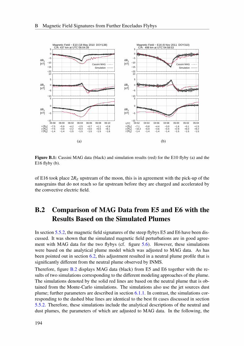
B Magnetic Field Signatures from Further Enceladus Flybys
−20
−15
−10
−5
0
5
05:58 06:00 06:02 06:04 06:06 06:08 06:10
Magnetic Field − E10 (18 May 2010 DOY138) C/A: 437 km at UTC 06:04:39
∆Bx [nT] Cassini MAG
Simulation
−10
−5
0
5
10
05:58 06:00 06:02 06:04 06:06 06:08 06:10
∆By [nT]
−10
−5
0
5
05:58 06:00 06:02 06:04 06:06 06:08 06:10x [RE]y [RE]z [RE]
−7.5−7.5−1.4
−5.9−4.9−1.4
−4.2−2.2−1.5
−2.5+0.4−1.5
−0.7+3.0−1.5
+1.1+5.5−1.5
+2.8+8.1−1.6
∆Bz [nT]
(a)
−20
−15
−10
−5
0
5
04:52 04:54 04:56 04:58 05:00 05:02 05:04
Magnetic Field − E16 (6 Nov 2011 DOY310) C/A: 498 km at UTC 04:58:53
∆Bx [nT] Cassini MAG
Simulation
−10
−5
0
5
10
04:52 04:54 04:56 04:58 05:00 05:02 05:04
∆By [nT]
−10
−5
0
5
04:52 04:54 04:56 04:58 05:00 05:02 05:04UTCx [RE]y [RE]z [RE]
−7.1−10.2−1.4
−5.8−6.9−1.4
−4.4−3.6−1.4
−3.0−0.4−1.4
−1.6+2.9−1.5
−0.1+6.0−1.5
+1.5+9.2−1.5
∆Bz [nT]
(b)
Figure B.1: Cassini MAG data (black) and simulation results (red) for the E10 flyby (a) and theE16 flyby (b).
of E16 took place 2RE upstream of the moon, this is in agreement with the pick-up of thenanograins that do not reach so far upstream before they are charged and accelerated bythe convective electric field.
B.2 Comparison of MAG Data from E5 and E6 with theResults Based on the Simulated Plumes
In section 5.5.2, the magnetic field signatures of the steep flybys E5 and E6 have been dis-cussed. It was shown that the simulated magnetic field perturbations are in good agree-ment with MAG data for the two flybys (cf. figure 5.6). However, these simulationswere based on the analytical plume model which was adjusted to MAG data. As hasbeen pointed out in section 6.2, this adjustment resulted in a neutral plume profile that issignificantly different from the neutral plume observed by INMS.Therefore, figure B.2 displays MAG data (black) from E5 and E6 together with the re-sults of two simulations corresponding to the different modeling approaches of the plume.The simulations denoted by the solid red lines are based on the neutral plume that is ob-tained from the Monte-Carlo simulations. The simulations also use the jet sources dustplume; further parameters are described in section 6.1.1. In contrast, the simulations cor-responding to the dashed blue lines are identical to the best fit cases discussed in section5.5.2. Therefore, these simulations include the analytical descriptions of the neutral anddust plumes, the parameters of which are adjusted to MAG data. In the following, the
194
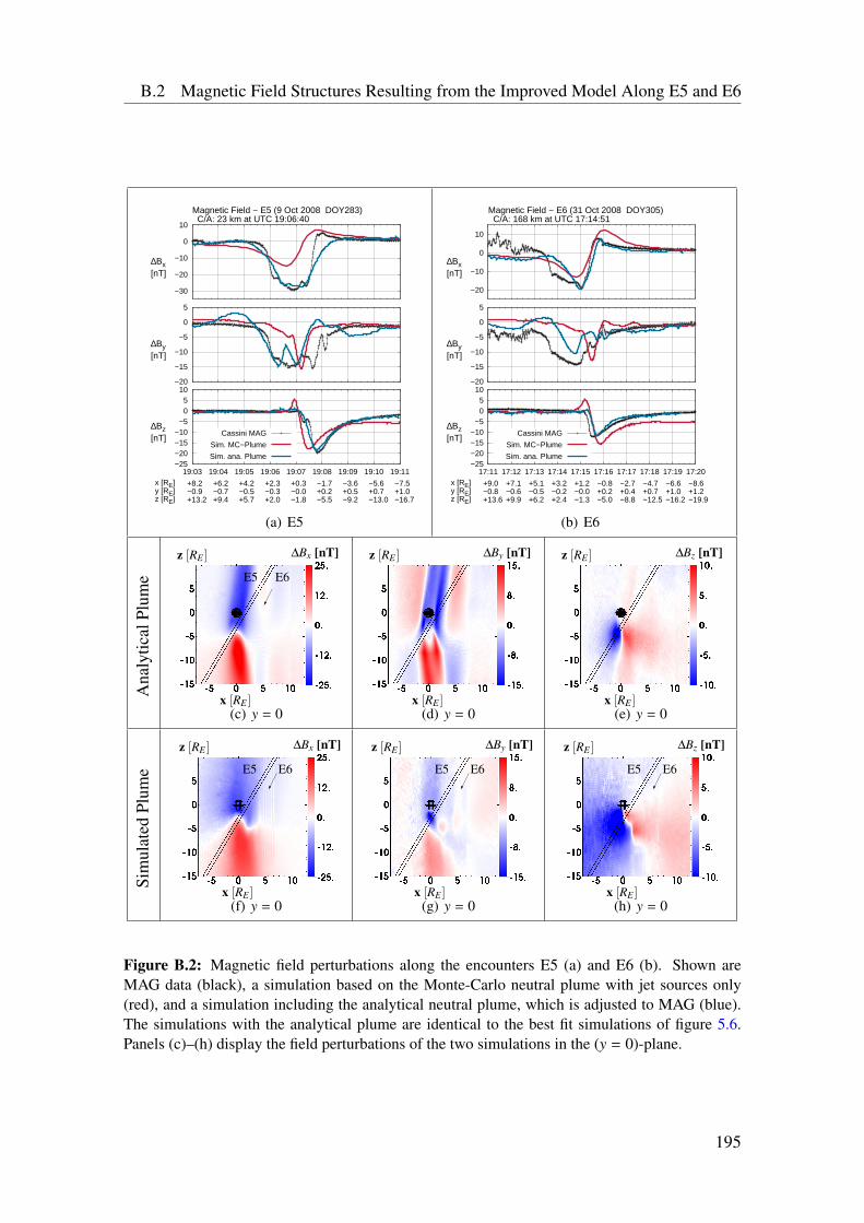
B.2 Magnetic Field Structures Resulting from the Improved Model Along E5 and E6
−30
−20
−10
0
10
19:03 19:04 19:05 19:06 19:07 19:08 19:09 19:10 19:11
Magnetic Field − E5 (9 Oct 2008 DOY283) C/A: 23 km at UTC 19:06:40
∆Bx [nT]
−20
−15
−10
−5
0
5
19:03 19:04 19:05 19:06 19:07 19:08 19:09 19:10 19:11
∆By [nT]
−25−20−15−10
−5 0 5
10
19:03 19:04 19:05 19:06 19:07 19:08 19:09 19:10 19:11x [RE]y [RE]z [RE]
+8.2−0.9+13.2
+6.2−0.7+9.4
+4.2−0.5+5.7
+2.3−0.3+2.0
+0.3−0.0−1.8
−1.7+0.2−5.5
−3.6+0.5−9.2
−5.6+0.7−13.0
−7.5+1.0−16.7
∆Bz [nT]
Cassini MAG
Sim. MC−Plume
Sim. ana. Plume
(a) E5
−20
−10
0
10
17:11 17:12 17:13 17:14 17:15 17:16 17:17 17:18 17:19 17:20
Magnetic Field − E6 (31 Oct 2008 DOY305) C/A: 168 km at UTC 17:14:51
∆Bx [nT]
−20
−15
−10
−5
0
5
17:11 17:12 17:13 17:14 17:15 17:16 17:17 17:18 17:19 17:20
∆By [nT]
−25−20−15−10
−5 0 5
10
17:11 17:12 17:13 17:14 17:15 17:16 17:17 17:18 17:19 17:20x [RE]y [RE]z [RE]
+9.0−0.8+13.6
+7.1−0.6+9.9
+5.1−0.5+6.2
+3.2−0.2+2.4
+1.2−0.0−1.3
−0.8+0.2−5.0
−2.7+0.4−8.8
−4.7+0.7−12.5
−6.6+1.0−16.2
−8.6+1.2−19.9
∆Bz [nT]
Cassini MAG
Sim. MC−Plume
Sim. ana. Plume
(b) E6
Ana
lytic
alPl
ume
E6E5
x [RE ]
z [RE ] ∆Bx [nT]
1
(c) y = 0x [RE ]
z [RE ] ∆By [nT]
1
(d) y = 0x [RE ]
z [RE ] ∆Bz [nT]
1
(e) y = 0
Sim
ulat
edPl
ume
E5 E6
x [RE ]
z [RE ] ∆Bx [nT]
1
(f) y = 0
E5 E6
x [RE ]
z [RE ] ∆By [nT]
1
(g) y = 0
E5 E6
x [RE ]
z [RE ] ∆Bz [nT]
1
(h) y = 0
Figure B.2: Magnetic field perturbations along the encounters E5 (a) and E6 (b). Shown areMAG data (black), a simulation based on the Monte-Carlo neutral plume with jet sources only(red), and a simulation including the analytical neutral plume, which is adjusted to MAG (blue).The simulations with the analytical plume are identical to the best fit simulations of figure 5.6.Panels (c)–(h) display the field perturbations of the two simulations in the (y = 0)-plane.
195
B Magnetic Field Signatures from Further Enceladus Flybys
two neutral plumes are referred to as ”analytical plume” and ”simulated or Monte-Carloplume”, respectively. Surprisingly, the agreement between MAG data and simulation forall three components is better for the simulation with the analytical plume than for thesimulation based on the Monte-Carlo plume.For a better understanding of the discrepancies between the simulated field perturbations,panels (c)–(h) of figure B.2 display the field perturbations in the (y = 0)-plane. The ana-lytical plume generates a sharply defined Alfvén flux tube with strong Bx and By perturba-tions, whereas the Monte-Carlo plume generates an Alfvén wing which exhibits a ratherdiffuse transition from the flux tube to the background. The By perturbation of the Alfvénwing triggered by the Monte-Carlo plume is even about 10 nT weaker than that of theAlfvén wing generated by the analytical plume. For both cases, the transition region from∆Bx < 0 to ∆Bx > 0 possesses the shape of a parabola that opens down. For the analyticalplume, this parabola is narrower and its vertex is located further south than for the simu-lated plume. In particular in the inbound region of the E5 trajectory, the observed Bx andBy perturbations agree better with the narrower Alfvén wing. Both, E5 and E6 intersectalso the southern Alfvén wing in the simulation with the Monte-Carlo plume, yielding adisagreement between simulation and data around 19:08 and 17:16, respectively. In the By
component, MAG data of both flybys show a perturbation of ∆By < −10 nT already aboveEnceladus, in agreement with the perturbation generated by the analytical plume. How-ever, the positive ∆By outside the Alfvén flux tube (cf. panel (d)) has not been observed.Furthermore, the results for the simulated plume show only a spiky decrease of By alongthe flybys, corresponding to the small region with ∆By ≈ −10 nT below Enceladus’ southpole (panel (g)). In contrast, MAG data exhibits an extended interval with ∆By < −10 nTfrom about z = +2RE to z = −5RE in rough agreement with the perturbations gener-ated by the analytical plume. The Bz perturbation generated by the Monte-Carlo plumeexhibits a significantly larger pile-up region (see panel (h)) than the simulation with theanalytical plume. In addition, the simulated neutral plume also leads to a short intervalwith a positive Bz perturbation of about ∆Bz = +5 nT along the flyby trajectories that wasnot observed by Cassini. This interval corresponds to the small region of positive ∆Bz
close to the south pole. As has been discussed in section 6.5.5, the field decrease regionis rotated out of Cassini’s path for the E14 and E19 flybys due to the modifications of thecurrent systems by the dust. Thus, minor changes in the shape of the dust plume may alsoresolve the discrepancy of the simulated Bz perturbations and MAG data along E5 and E6.However, the narrower analytical plume shifted both, pile-up and field decrease furthersouthward and in consequence, these simulations do not exhibit a positive ∆Bz along E5and E6.Overall, the magnetic field structures generated by the narrower and denser analyticalplume match well with MAG data, whereas a neutral plume in agreement with INMSdata fails to explain several features of the observed magnetic field perturbations. Thus itseems to be challenging to find a parameter setup which is in agreement with both, MAGand INMS data for E5 and E6. Although not shown here, modeling of the two other steepflybys E3 and E4 led to the same difficulties. To resolve this issue, several explanationscould be considered:
• A different orientation of the jets may lead to a narrower plume along the trajecto-ries. However, this is rather unlikely, since the neutral density of the Monte-Carlo
196
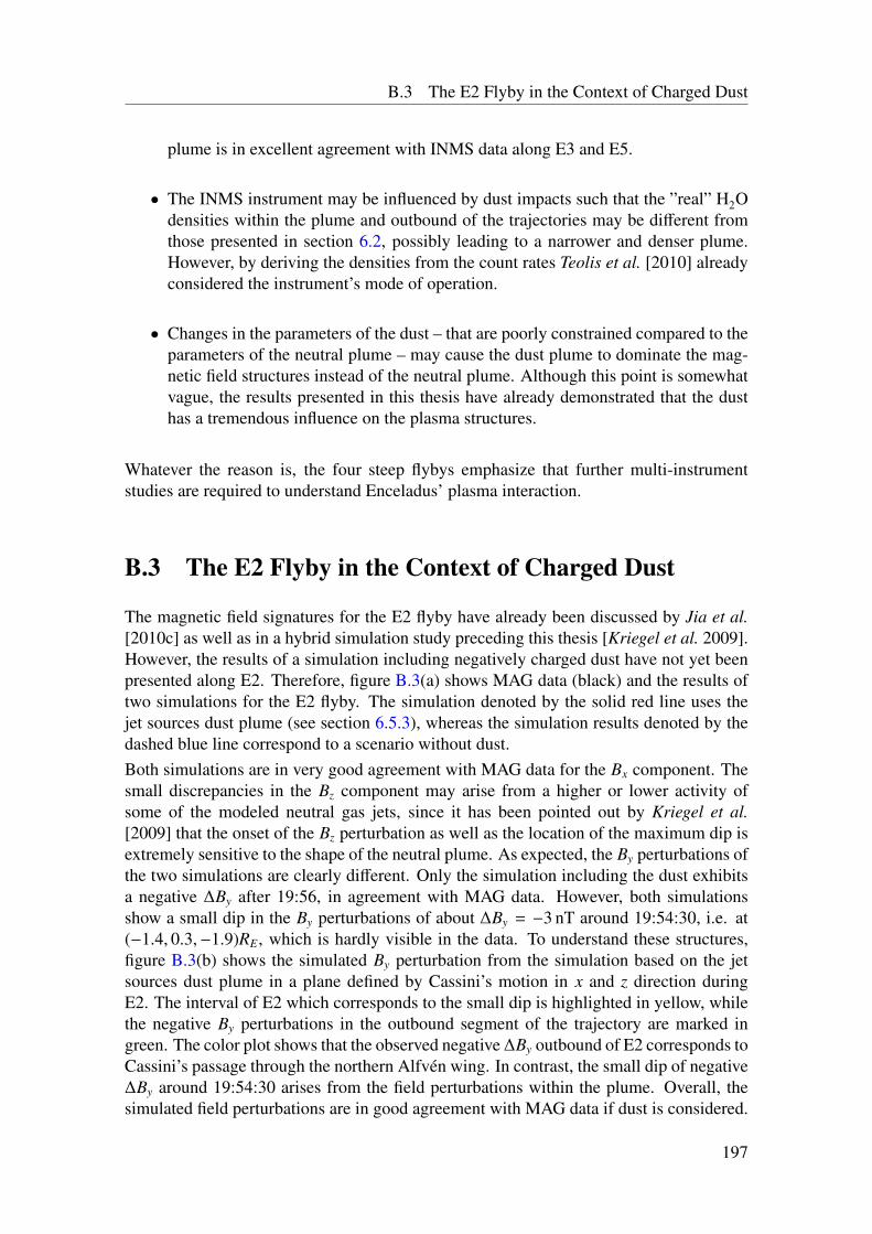
B.3 The E2 Flyby in the Context of Charged Dust
plume is in excellent agreement with INMS data along E3 and E5.
• The INMS instrument may be influenced by dust impacts such that the ”real” H2Odensities within the plume and outbound of the trajectories may be different fromthose presented in section 6.2, possibly leading to a narrower and denser plume.However, by deriving the densities from the count rates Teolis et al. [2010] alreadyconsidered the instrument’s mode of operation.
• Changes in the parameters of the dust – that are poorly constrained compared to theparameters of the neutral plume – may cause the dust plume to dominate the mag-netic field structures instead of the neutral plume. Although this point is somewhatvague, the results presented in this thesis have already demonstrated that the dusthas a tremendous influence on the plasma structures.
Whatever the reason is, the four steep flybys emphasize that further multi-instrumentstudies are required to understand Enceladus’ plasma interaction.
B.3 The E2 Flyby in the Context of Charged Dust
The magnetic field signatures for the E2 flyby have already been discussed by Jia et al.[2010c] as well as in a hybrid simulation study preceding this thesis [Kriegel et al. 2009].However, the results of a simulation including negatively charged dust have not yet beenpresented along E2. Therefore, figure B.3(a) shows MAG data (black) and the results oftwo simulations for the E2 flyby. The simulation denoted by the solid red line uses thejet sources dust plume (see section 6.5.3), whereas the simulation results denoted by thedashed blue line correspond to a scenario without dust.Both simulations are in very good agreement with MAG data for the Bx component. Thesmall discrepancies in the Bz component may arise from a higher or lower activity ofsome of the modeled neutral gas jets, since it has been pointed out by Kriegel et al.[2009] that the onset of the Bz perturbation as well as the location of the maximum dip isextremely sensitive to the shape of the neutral plume. As expected, the By perturbations ofthe two simulations are clearly different. Only the simulation including the dust exhibitsa negative ∆By after 19:56, in agreement with MAG data. However, both simulationsshow a small dip in the By perturbations of about ∆By = −3 nT around 19:54:30, i.e. at(−1.4, 0.3,−1.9)RE, which is hardly visible in the data. To understand these structures,figure B.3(b) shows the simulated By perturbation from the simulation based on the jetsources dust plume in a plane defined by Cassini’s motion in x and z direction duringE2. The interval of E2 which corresponds to the small dip is highlighted in yellow, whilethe negative By perturbations in the outbound segment of the trajectory are marked ingreen. The color plot shows that the observed negative ∆By outbound of E2 corresponds toCassini’s passage through the northern Alfvén wing. In contrast, the small dip of negative∆By around 19:54:30 arises from the field perturbations within the plume. Overall, thesimulated field perturbations are in good agreement with MAG data if dust is considered.
197
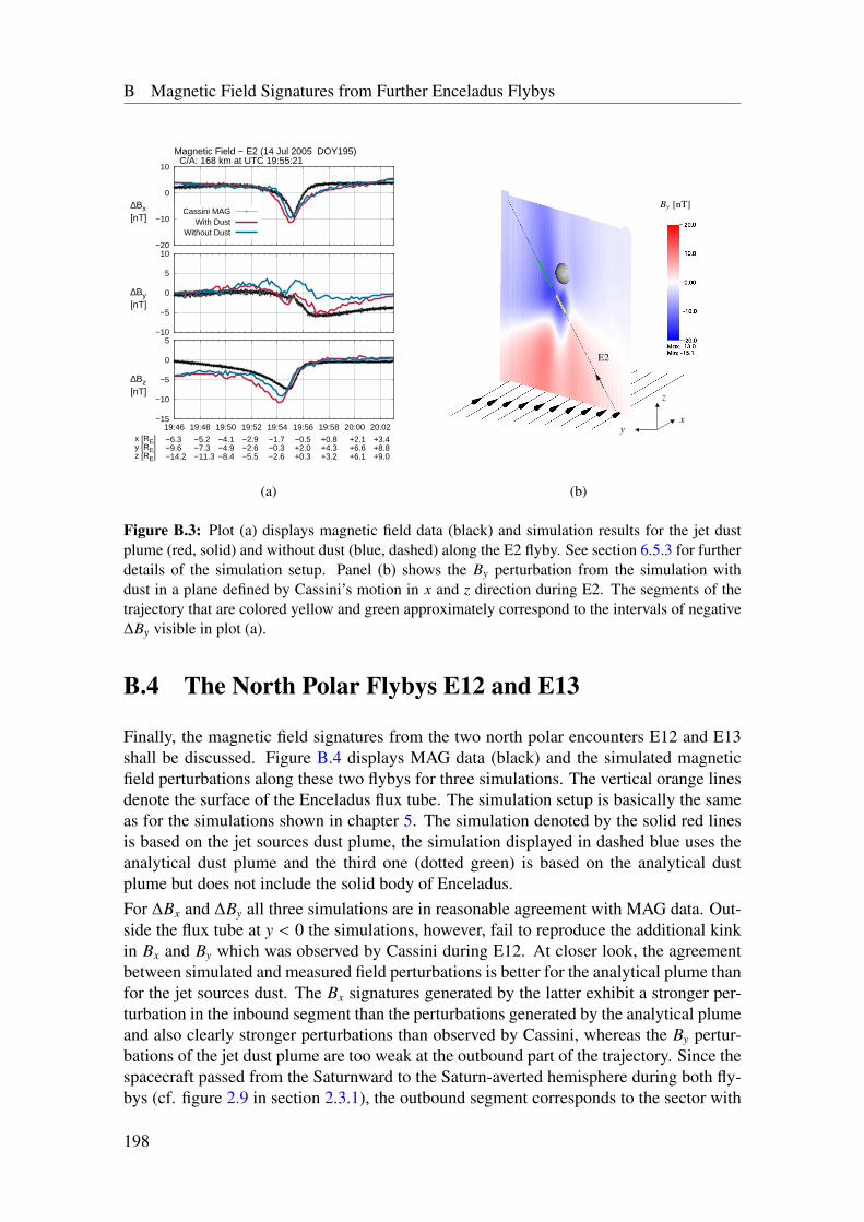
B Magnetic Field Signatures from Further Enceladus Flybys
−20
−10
0
10
19:46 19:48 19:50 19:52 19:54 19:56 19:58 20:00 20:02
Magnetic Field − E2 (14 Jul 2005 DOY195) C/A: 168 km at UTC 19:55:21
∆Bx [nT]
Cassini MAGWith Dust
Without Dust
−10
−5
0
5
10
19:46 19:48 19:50 19:52 19:54 19:56 19:58 20:00 20:02
∆By [nT]
−15
−10
−5
0
5
19:46 19:48 19:50 19:52 19:54 19:56 19:58 20:00 20:02x [RE]y [RE]z [RE]
−6.3−9.6−14.2
−5.2−7.3−11.3
−4.1−4.9−8.4
−2.9−2.6−5.5
−1.7−0.3−2.6
−0.5+2.0+0.3
+0.8+4.3+3.2
+2.1+6.6+6.1
+3.4+8.8+9.0
∆Bz [nT]
(a)
By [nT]
E2
y
z
x
(b)
Figure B.3: Plot (a) displays magnetic field data (black) and simulation results for the jet dustplume (red, solid) and without dust (blue, dashed) along the E2 flyby. See section 6.5.3 for furtherdetails of the simulation setup. Panel (b) shows the By perturbation from the simulation withdust in a plane defined by Cassini’s motion in x and z direction during E2. The segments of thetrajectory that are colored yellow and green approximately correspond to the intervals of negative∆By visible in plot (a).
B.4 The North Polar Flybys E12 and E13
Finally, the magnetic field signatures from the two north polar encounters E12 and E13shall be discussed. Figure B.4 displays MAG data (black) and the simulated magneticfield perturbations along these two flybys for three simulations. The vertical orange linesdenote the surface of the Enceladus flux tube. The simulation setup is basically the sameas for the simulations shown in chapter 5. The simulation denoted by the solid red linesis based on the jet sources dust plume, the simulation displayed in dashed blue uses theanalytical dust plume and the third one (dotted green) is based on the analytical dustplume but does not include the solid body of Enceladus.For ∆Bx and ∆By all three simulations are in reasonable agreement with MAG data. Out-side the flux tube at y < 0 the simulations, however, fail to reproduce the additional kinkin Bx and By which was observed by Cassini during E12. At closer look, the agreementbetween simulated and measured field perturbations is better for the analytical plume thanfor the jet sources dust. The Bx signatures generated by the latter exhibit a stronger per-turbation in the inbound segment than the perturbations generated by the analytical plumeand also clearly stronger perturbations than observed by Cassini, whereas the By pertur-bations of the jet dust plume are too weak at the outbound part of the trajectory. Since thespacecraft passed from the Saturnward to the Saturn-averted hemisphere during both fly-bys (cf. figure 2.9 in section 2.3.1), the outbound segment corresponds to the sector with
198
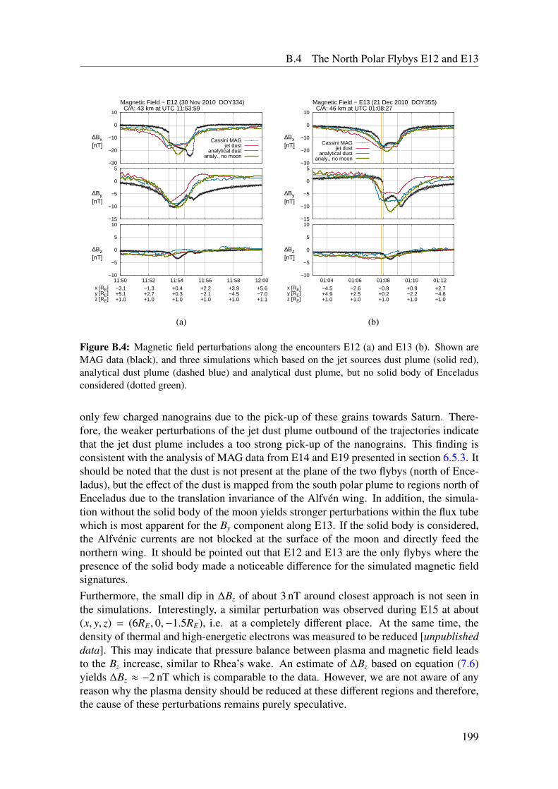
B.4 The North Polar Flybys E12 and E13
−30
−20
−10
0
10
11:50 11:52 11:54 11:56 11:58 12:00
Magnetic Field − E12 (30 Nov 2010 DOY334) C/A: 43 km at UTC 11:53:59
∆Bx [nT]
Cassini MAGjet dust
analytical dustanaly., no moon
−15
−10
−5
0
5
11:50 11:52 11:54 11:56 11:58 12:00
∆By [nT]
−10
−5
0
5
10
11:50 11:52 11:54 11:56 11:58 12:00x [RE]y [RE]z [RE]
−3.1+5.1+1.0
−1.3+2.7+1.0
+0.4+0.3+1.0
+2.2−2.1+1.0
+3.9−4.5+1.0
+5.6−7.0+1.1
∆Bz [nT]
(a)
−30
−20
−10
0
10
01:04 01:06 01:08 01:10 01:12
Magnetic Field − E13 (21 Dec 2010 DOY355) C/A: 46 km at UTC 01:08:27
∆Bx [nT] Cassini MAG
jet dustanalytical dust
analy., no moon
−15
−10
−5
0
5
01:04 01:06 01:08 01:10 01:12
∆By [nT]
−10
−5
0
5
10
01:04 01:06 01:08 01:10 01:12x [RE]y [RE]z [RE]
−4.5+4.9+1.0
−2.6+2.5+1.0
−0.9+0.2+1.0
+0.9−2.2+1.0
+2.7−4.6+1.0
∆Bz [nT]
(b)
Figure B.4: Magnetic field perturbations along the encounters E12 (a) and E13 (b). Shown areMAG data (black), and three simulations which based on the jet sources dust plume (solid red),analytical dust plume (dashed blue) and analytical dust plume, but no solid body of Enceladusconsidered (dotted green).
only few charged nanograins due to the pick-up of these grains towards Saturn. There-fore, the weaker perturbations of the jet dust plume outbound of the trajectories indicatethat the jet dust plume includes a too strong pick-up of the nanograins. This finding isconsistent with the analysis of MAG data from E14 and E19 presented in section 6.5.3. Itshould be noted that the dust is not present at the plane of the two flybys (north of Ence-ladus), but the effect of the dust is mapped from the south polar plume to regions north ofEnceladus due to the translation invariance of the Alfvén wing. In addition, the simula-tion without the solid body of the moon yields stronger perturbations within the flux tubewhich is most apparent for the By component along E13. If the solid body is considered,the Alfvénic currents are not blocked at the surface of the moon and directly feed thenorthern wing. It should be pointed out that E12 and E13 are the only flybys where thepresence of the solid body made a noticeable difference for the simulated magnetic fieldsignatures.Furthermore, the small dip in ∆Bz of about 3 nT around closest approach is not seen inthe simulations. Interestingly, a similar perturbation was observed during E15 at about(x, y, z) = (6RE, 0,−1.5RE), i.e. at a completely different place. At the same time, thedensity of thermal and high-energetic electrons was measured to be reduced [unpublisheddata]. This may indicate that pressure balance between plasma and magnetic field leadsto the Bz increase, similar to Rhea’s wake. An estimate of ∆Bz based on equation (7.6)yields ∆Bz ≈ −2 nT which is comparable to the data. However, we are not aware of anyreason why the plasma density should be reduced at these different regions and therefore,the cause of these perturbations remains purely speculative.
199

C Simulations of the Dione D3 Flyby
Apart from Enceladus and Rhea, we also briefly studied the third largest icy satellite Dione(RD = 561.5 km) which orbits Saturn at a distance of about 6.28RS , between the orbitsof Tethys and Rhea. So far, Cassini performed three targeted flybys of Dione, labeledD1, D2 and D3. The magnetic field data obtained during the first two flybys have beenanalyzed by Simon et al. [2011a] who found that the signatures from D1 are consistentwith the existence of a tenuous, sputtering-induced atmosphere around Dione.We applied A.I.K.E.F. to the plasma interaction of Dione in order to contribute to the ana-lysis of Energetic particle measurements in the vicinity of Dione by Krupp et al. [2013]1.These authors compared electron absorption signatures from measurements of the CassiniLEMMS instrument with electron wake profiles resulting from electron guiding centertrajectory tracings in our simulated environment of Dione.The simulation was adjusted to the D3 flyby which occurred on 12 December 2011. Thetrajectory is shown in figure C.1 in the Dione Interaction System, which can be intro-duced in analogy to the ENIS and the RHIS (see section 2.3). The encounter passedthrough Dione’s wake in the anti-Saturnward direction parallel to the equatorial plane atz = 0.1RD. The closest approach altitude was only about 100 km.The parameters applied in the simulation are summarized in Table C.1. In agreement withRPWS measurements of the upper hybrid frequency at Dione’s L-shell [Gurnett et al.2007, Persoon et al. 2009], an upstream plasma density of n0 = 25 cm−3 is used. Theplasma is assumed to consist of water group ions with an average mass of mi = 17 amuwhich impinge on the moon at the ideal corotation velocity of u0 = 40 cm−3. The electrontemperature is set to kBTec = 6 eV, and the ion temperature is kBTi = 90 eV [Khurana et al.2008]. The background magnetic field is modeled as a dipole field and is adjusted to MAGdata from the D3 flyby (cf. Figure C.2). Like Enceladus and Rhea, Dione itself is modeledas an absorbing and insulating body (see section 4.5.1). The conductivity of the interior isset toσ = 1·10−7 S/m. The simulation box has a size of Lx×Ly×Lz = 18RD×15RD×15 RD.Two levels of refinement are used, yielding a resolution of ∆L2 ≈ 0.05RDi = 28 km.Further numerical parameters are provided in table C.1.An overview of our simulation results is provided in figure C.3. Panels C.3(a)–(c) showthe magnetic field perturbations in the y = 0 cross section, panels C.3(j)–(l) display theplane z = 0 and in panels (m)–(o) the results are are shown at z = +0.1RD, i.e. approx-
1Full reference: Krupp, N., E. Roussos, H. Kriegel, P. Kollmann, M.G. Kivelson, A. Kotova ,C. Paranicas, D.G. Mitchell, S.M. Krimigis, K.K. Khurana (2013), Energetic particle measurementsin the vicinity of Dione during the three Cassini encounters 2005–2011, Icarus, 226, 617–628, doi:10.1016/j.icarus.2013.06.007
201
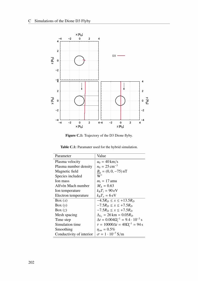
C Simulations of the Dione D3 Flyby
−4
−2
0
2
4
−4 −2 0 2 4
y [R
D]
x [RD]
−4
−2
0
2
4
−4 −2 0 2 4
y [R
D]
x [RD]−4 −2 0 2 4
−4
−2
0
2
4
y [RD ]
z [RD]−4 −2 0 2 4
−4
−2
0
2
4
y [RD ]
z [RD]
−4
−2
0
2
4−4 −2 0 2 4
z [R
D]
x [RD]
−4
−2
0
2
4−4 −2 0 2 4
z [R
D]
x [RD]
D3
Figure C.1: Trajectory of the D3 Dione flyby.
Table C.1: Paramater used for the hybrid simulation.
Parameter ValuePlasma velocity u0 = 40 km/sPlasma number density n0 = 25 cm−3
Magnetic field B0 = (0, 0,−75) nTSpecies included W+
Ion mass mi = 17 amuAlfvén Mach number MA = 0.63Ion temperature kBTi = 90 eVElectron temperature kBTe = 6 eVBox (x) −4.5RD ≤ x ≤ +13.5RD
Box (y) −7.5RD ≤ x ≤ +7.5RD
Box (z) −7.5RD ≤ x ≤ +7.5RD
Mesh spacing ∆L2 = 26 km = 0.05RD
Time step ∆t = 0.004Ω−1i = 9.4 · 10−3 s
Simulation time τ = 10000∆t = 40Ω−1i = 94 s
Smoothing ηsm = 0.5%Conductivity of interior σ = 1 · 10−7 S/m
202
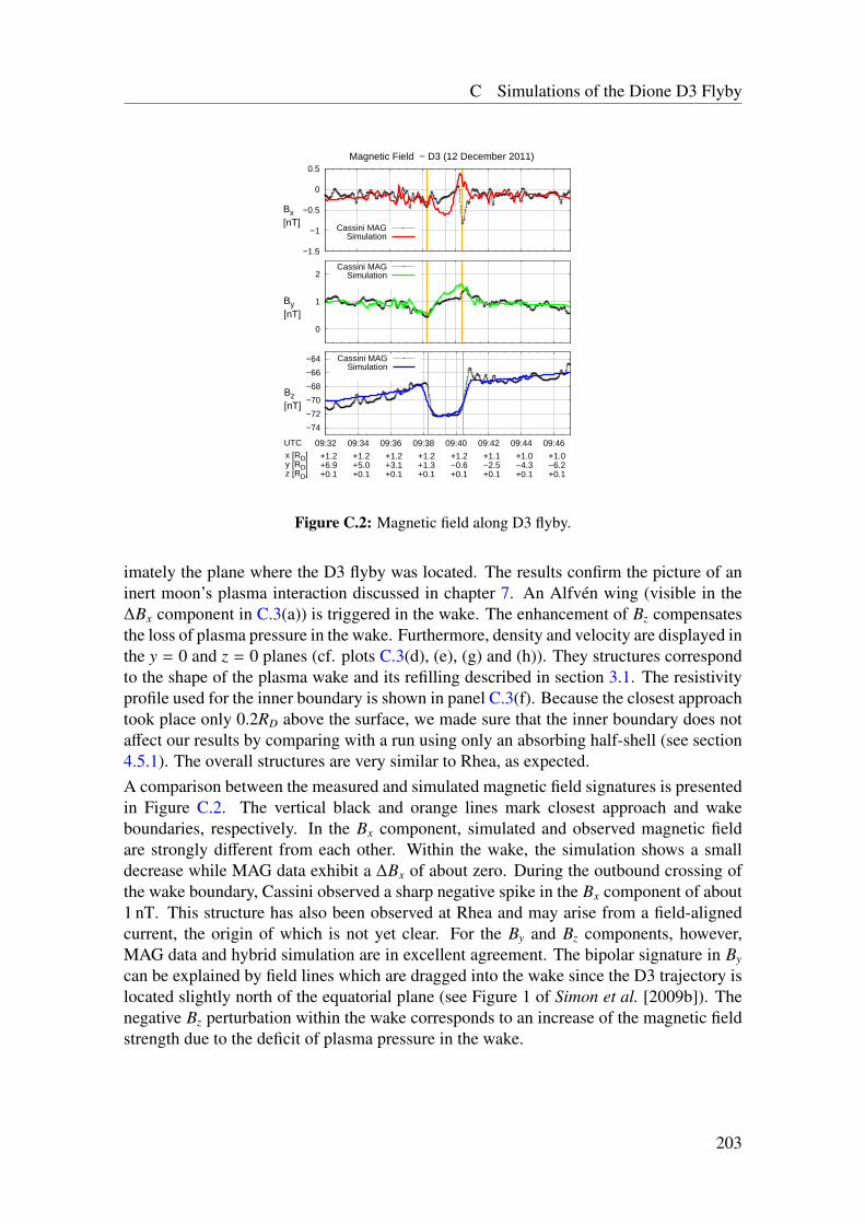
C Simulations of the Dione D3 Flyby
−1.5
−1
−0.5
0
0.5
09:32 09:34 09:36 09:38 09:40 09:42 09:44 09:46
Magnetic Field − D3 (12 December 2011)
Bx [nT] Cassini MAG
Simulation
0
1
2
09:32 09:34 09:36 09:38 09:40 09:42 09:44 09:46
By [nT]
Cassini MAGSimulation
−74
−72
−70
−68
−66
−64
09:32 09:34 09:36 09:38 09:40 09:42 09:44 09:46UTCx [RD]y [RD]z [RD]
+1.2+6.9+0.1
+1.2+5.0+0.1
+1.2+3.1+0.1
+1.2+1.3+0.1
+1.2−0.6+0.1
+1.1−2.5+0.1
+1.0−4.3+0.1
+1.0−6.2+0.1
Bz [nT]
Cassini MAGSimulation
Figure C.2: Magnetic field along D3 flyby.
imately the plane where the D3 flyby was located. The results confirm the picture of aninert moon’s plasma interaction discussed in chapter 7. An Alfvén wing (visible in the∆Bx component in C.3(a)) is triggered in the wake. The enhancement of Bz compensatesthe loss of plasma pressure in the wake. Furthermore, density and velocity are displayed inthe y = 0 and z = 0 planes (cf. plots C.3(d), (e), (g) and (h)). They structures correspondto the shape of the plasma wake and its refilling described in section 3.1. The resistivityprofile used for the inner boundary is shown in panel C.3(f). Because the closest approachtook place only 0.2RD above the surface, we made sure that the inner boundary does notaffect our results by comparing with a run using only an absorbing half-shell (see section4.5.1). The overall structures are very similar to Rhea, as expected.A comparison between the measured and simulated magnetic field signatures is presentedin Figure C.2. The vertical black and orange lines mark closest approach and wakeboundaries, respectively. In the Bx component, simulated and observed magnetic fieldare strongly different from each other. Within the wake, the simulation shows a smalldecrease while MAG data exhibit a ∆Bx of about zero. During the outbound crossing ofthe wake boundary, Cassini observed a sharp negative spike in the Bx component of about1 nT. This structure has also been observed at Rhea and may arise from a field-alignedcurrent, the origin of which is not yet clear. For the By and Bz components, however,MAG data and hybrid simulation are in excellent agreement. The bipolar signature in By
can be explained by field lines which are dragged into the wake since the D3 trajectory islocated slightly north of the equatorial plane (see Figure 1 of Simon et al. [2009b]). Thenegative Bz perturbation within the wake corresponds to an increase of the magnetic fieldstrength due to the deficit of plasma pressure in the wake.
203
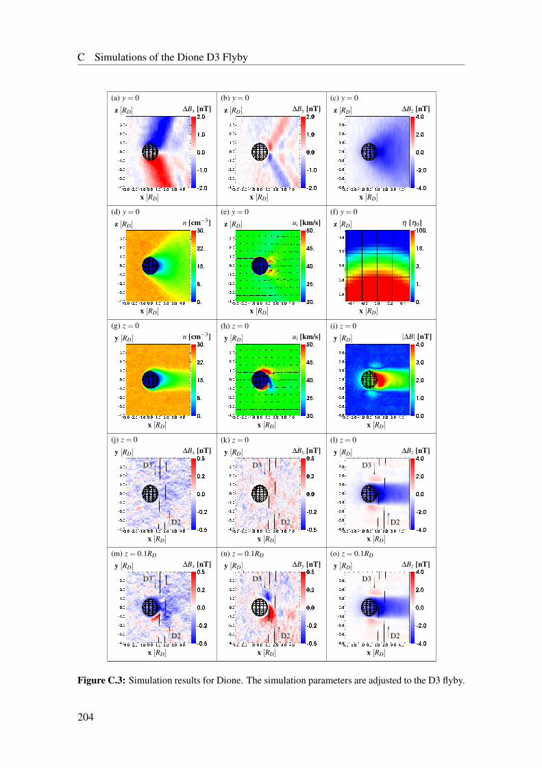
C Simulations of the Dione D3 Flyby
(a) y = 0
x [RD]
z [RD] ∆Bx [nT]
1
(b) y = 0
x [RD]
z [RD] ∆By [nT]
1
(c) y = 0
x [RD]
z [RD] ∆Bz [nT]
1
(d) y = 0
x [RD]
z [RD] n [cm−3]
1
(e) y = 0
x [RD]
z [RD] ui [km/s]
1
(f) y = 0
x [RD]
z [RD] η [η0]
1
(g) z = 0
x [RD]
y [RD] n [cm−3]
1
(h) z = 0
x [RD]
y [RD] ui [km/s]
1
(i) z = 0
x [RD]
y [RD] |∆B| [nT]
1
(j) z = 0
D2
CCCW
D3
x [RD]
y [RD] ∆Bx [nT]
1
(k) z = 0
D2
CCCW
D3
x [RD]
y [RD] ∆By [nT]
1
(l) z = 0
D2
CCCW
D3
x [RD]
y [RD] ∆Bz [nT]
1
(m) z = 0.1RD
D2
CCCW
D3
x [RD]
y [RD] ∆Bx [nT]
1
(n) z = 0.1RD
D2
CCCW
D3
x [RD]
y [RD] ∆By [nT]
1
(o) z = 0.1RD
D2
CCCW
D3
x [RD]
y [RD] ∆Bz [nT]
1Figure C.3: Simulation results for Dione. The simulation parameters are adjusted to the D3 flyby.
204
Bibliography
Anderson, J. D., and G. Schubert (2007), Saturn’s satellite Rhea is a homogeneous mix ofrock and ice, Geophysical Research Letters, 34, 2202, doi: 10.1029/2006GL028100.
André, N., et al. (2008), Identification of Saturn’s magnetospheric regions and associatedplasma processes: Synopsis of Cassini observations during orbit insertion, Reviews ofGeophysics, 46, RG4008, doi: 10.1029/2007RG000238.
Andrews, D. J., A. J. Coates, S. W. H. Cowley, M. K. Dougherty, L. Lamy, G. Provan, andP. Zarka (2010), Magnetospheric period oscillations at Saturn: Comparison of equa-torial and high-latitude magnetic field periods with north and south Saturn kilometricradiation periods, Journal of Geophysical Research (Space Physics), 115, A12252, doi:10.1029/2010JA015666.
Andrews, D. J., B. Cecconi, S. W. H. Cowley, M. K. Dougherty, L. Lamy, G. Provan,and P. Zarka (2011), Planetary period oscillations in Saturn’s magnetosphere: Evi-dence in magnetic field phase data for rotational modulation of Saturn kilometric radi-ation emissions, Journal of Geophysical Research (Space Physics), 116, A09206, doi:10.1029/2011JA016636.
Arridge, C. S., C. T. Russell, K. K. Khurana, N. Achilleos, N. André, A. M. Rymer, M. K.Dougherty, and A. J. Coates (2007), Mass of Saturn’s magnetodisc: Cassini observa-tions, Geophysical Research Letters, 34, L09108, doi: 10.1029/2006GL028921.
Bagdonat, T. (2004), Hybrid Simulation of Weak Comets, Ph.D. thesis, TU Braun-schweig.
Bagdonat, T., and U. Motschmann (2002a), From a Weak to a Strong Comet - 3dGlobal Hybrid Simulation Studies, Earth Moon and Planets, 90, 305–321, doi:10.1023/A:1021578232282.
Bagdonat, T., and U. Motschmann (2002b), 3D Hybrid Simulation Code UsingCurvilinear Coordinates, Journal of Computational Physics, 183, 470–485, doi:10.1006/jcph.2002.7203.
Birch, P. C., and S. C. Chapman (2001), Detailed structure and dynamics in particle-in-cell simulations of the lunar wake, Physics of Plasmas, 8, 4551–4559, doi:10.1063/1.1398570.
Blöcker, A. (2013), MHD-Modellierung der Plasmawechselwirkung bei Io und Ence-ladus, Master’s thesis, Universität zu Köln.
205
Bibliography
Bonfond, B., D. Grodent, J.-C. Gérard, A. Radioti, J. Saur, and S. Jacobsen (2008), UVIo footprint leading spot: A key feature for understanding the UV Io footprint multi-plicity?, Geophysical Research Letters, 35, L05107, doi: 10.1029/2007GL032418.
Bonfond, B., D. Grodent, J.-C. Gérard, A. Radioti, V. Dols, P. A. Delamere, and J. T.Clarke (2009), The Io UV footprint: Location, inter-spot distances and tail verti-cal extent, Journal of Geophysical Research (Space Physics), 114, A07224, doi:10.1029/2009JA014312.
Bößwetter, A., T. Bagdonat, U. Motschmann, and K. Sauer (2004), Plasma boundaries atMars: a 3-D simulation study, Annales Geophysicae, 22(12), 4363–4379.
Burch, J. L., J. Goldstein, W. S. Lewis, D. T. Young, A. J. Coates, M. K. Dougherty, andN. André (2007), Tethys and Dione as sources of outward-flowing plasma in Saturn’smagnetosphere, Nature, 447, 833–835, doi: 10.1038/nature05906.
Burger, M. H., E. C. Sittler, R. E. Johnson, H. T. Smith, O. J. Tucker, and V. I. Shema-tovich (2007), Understanding the escape of water from Enceladus, Journal of Geophys-ical Research (Space Physics), 112, A06,219, doi: 10.1029/2006JA012086.
Burton, M. E., M. K. Dougherty, and C. T. Russell (2010), Saturn’s inter-nal planetary magnetic field, Geophysical Research Letters, 37, L24105, doi:10.1029/2010GL045148.
Behounková, M., G. Tobie, G. Choblet, and O. Cadek (2012), Tidally-induced meltingevents as the origin of south-pole activity on Enceladus, Icarus, 219, 655–664, doi:10.1016/j.icarus.2012.03.024.
Cao, H., C. T. Russell, U. R. Christensen, M. K. Dougherty, and M. E. Burton (2011),Saturn’s very axisymmetric magnetic field: No detectable secular variation or tilt, Earthand Planetary Science Letters, 304(1 – 2), 22 – 28, doi: 10.1016/j.epsl.2011.02.035.
Clarke, J. T., D. Grodent, S. W. H. Cowley, E. J. Bunce, P. Zarka, J. E. P. Connerney,and T. Satoh (2004), Jupiter. The Planet, Satellites and Magnetosphere, chap. Jupiter’saurora, pp. 639–670, Cambridge Univ. Press.
Coates, A. J., G. H. Jones, G. R. Lewis, A. Wellbrock, D. T. Young, F. J. Crary, R. E.Johnson, T. A. Cassidy, and T. W. Hill (2010), Negative ions in the Enceladus plume,Icarus, 206, 618–622, doi: 10.1016/j.icarus.2009.07.013.
Coates, A. J., A. Wellbrock, G. H. Jones, J. H. Waite, P. Schippers, M. F. Thomsen, C. S.Arridge, and R. L. Tokar (2013), Photoelectrons in the Enceladus plume, Journal ofGeophysical Research (Space Physics), 118, 5099–5108, doi: 10.1002/jgra.50495.
Colburn, D. S., R. G. Currie, J. D. Mihalov, and C. P. Sonett (1967), Diamagnetic Solar-Wind Cavity Discovered behind Moon, Science, 158, 1040–1042, doi: 10.1126/sci-ence.158.3804.1040.
206
Bibliography
Cravens, T. E., R. L. McNutt, J. H. Waite, I. P. Robertson, J. G. Luhmann, W. Kasprzak,and W.-H. Ip (2009), Plume ionosphere of Enceladus as seen by the Cassini Ionand Neutral Mass Spectrometer, Geophysical Research Letters, 36, L08106, doi:10.1029/2009GL037811.
Cravens, T. E., N. Ozak, M. S. Richard, M. E. Campbell, I. P. Robertson, M. Perry, andA. M. Rymer (2011), Electron energetics in the Enceladus torus, Journal of Geophysi-cal Research (Space Physics), 116, A09205, doi: 10.1029/2011JA016498.
Desch, M. D., and M. L. Kaiser (1981), Voyager measurement of the rotation pe-riod of Saturn’s magnetic field, Geophysical Research Letters, 8, 253–256, doi:10.1029/GL008i003p00253.
Dong, Y., T. W. Hill, B. D. Teolis, B. A. Magee, and J. H. Waite (2011), The water vaporplumes of Enceladus, Journal of Geophysical Research (Space Physics), 116, A10204,doi: 10.1029/2011JA016693.
Dougherty, M. K., et al. (2004), The Cassini Magnetic Field Investigation, Space ScienceReviews, 114, 331–383, doi: 10.1007/s11214-004-1432-2.
Dougherty, M. K., et al. (2005), Cassini Magnetometer Observations During Saturn OrbitInsertion, Science, 307, 1266–1270, doi: 10.1126/science.1106098.
Dougherty, M. K., K. K. Khurana, F. M. Neubauer, C. T. Russell, J. Saur, J. S. Leisner,and M. E. Burton (2006), Identification of a Dynamic Atmosphere at Enceladus withthe Cassini Magnetometer, Science, 311, 1406–1409, doi: 10.1126/science.1120985.
Farrell, W. M., W. S. Kurth, D. A. Gurnett, R. E. Johnson, M. L. Kaiser, J. Wahlund,and J. H. Waite (2009), Electron density dropout near Enceladus in the contextof water-vapor and water-ice, Geophysical Research Letters, 36, L10,203, doi:10.1029/2008GL037108.
Farrell, W. M., et al. (2010), Modification of the plasma in the near-vicinity of Ence-ladus by the enveloping dust, Geophysical Research Letters, 37, L20,202, doi:10.1029/2010GL044768.
Fleshman, B. L., P. A. Delamere, and F. Bagenal (2010a), Modeling the Ence-ladus plume-plasma interaction, Geophysical Research Letters, 37, 3202–+, doi:10.1029/2009GL041613.
Fleshman, B. L., P. A. Delamere, and F. Bagenal (2010b), A sensitivity study ofthe Enceladus torus, Journal of Geophysical Research (Planets), 115, E04,007, doi:10.1029/2009JE003372.
Goertz, C. K. (1980), Io’s interaction with the plasma torus, Journal of Geophysical Re-search (Space Physics), 85, 2949–2956, doi: 10.1029/JA085iA06p02949.
Goldreich, P., and D. Lynden-Bell (1969), Io, a Jovian unipolar inductor, AstrophysicalJournal, 156, 59–78, doi: 10.1086/149947.
207
Bibliography
Gombosi, T. I., T. P. Armstrong, C. S. Arridge, K. K. Khurana, S. M. Krimigis, N. Krupp,A. M. Persoon, and M. F. Thomsen (2009), Saturn’s Magnetospheric Configuration, p.203, doi: 10.1007/978-1-4020-9217-6_9.
Gurnett, D. A., and W. R. Pryor (2012), Auroral Processes Associated With Saturn’sMoon Enceladus, Washington DC American Geophysical Union Geophysical Mono-graph Series, 197, 305–313, doi: 10.1029/2011GM001174.
Gurnett, D. A., A. M. Persoon, W. S. Kurth, J. B. Groene, T. F. Averkamp, M. K.Dougherty, and D. J. Southwood (2007), The Variable Rotation Period of the Inner Re-gion of Saturn’s Plasma Disk, Science, 316(5823), 442, doi: 10.1126/science.1138562.
Gurnett, D. A., et al. (2011), Auroral hiss, electron beams and standing Alfvén wavecurrents near Saturn’s moon Enceladus, Geophysical Research Letters, 38, L06,102,doi: 10.1029/2011GL046854.
Gustafsson, G., and J.-E. Wahlund (2010), Electron temperatures in Saturn’s plasma disc,Planet. Space Sci., 58, 1018–1025, doi: 10.1016/j.pss.2010.03.007.
Haff, P. K., G. L. Siscoe, and A. Eviatar (1983), Ring and plasma - The enigmae ofEnceladus, Icarus, 56, 426–438, doi: 10.1016/0019-1035(83)90164-1.
Hansen, C. J., L. Esposito, A. I. F. Stewart, J. Colwell, A. Hendrix, W. Pryor, D. Sheman-sky, and R. West (2006), Enceladus’ Water Vapor Plume, Science, 311, 1422–1425,doi: 10.1126/science.1121254.
Hansen, C. J., et al. (2008), Water vapour jets inside the plume of gas leaving Enceladus,Nature, 456, 477–479, doi: 10.1038/nature07542.
Hansen, C. J., D. E. Shemansky, L. W. Esposito, I. Stewart, and A. R. Hendrix (2010),The Composition and Structure of Enceladus’ Plume from a Cassini UVIS Observationof a Solar Occultation, AGU Fall Meeting Abstracts, pp. C9+.
Hansen, C. J., et al. (2011), The composition and structure of the Enceladus plume, Geo-physical Research Letters, 38, L11,202, doi: 10.1029/2011GL047415.
Harms, E. (2010), Modellierung des Plumes von Enceladus, Master’s thesis, TU Braun-schweig.
Hartogh, P., et al. (2011), Direct detection of the Enceladus water torus with Herschel,Astronomy & Astrophysics, 532, L2, doi: 10.1051/0004-6361/201117377.
Havnes, O., G. E. Morfill, and C. K. Goertz (1984), Plasma potential and grain chargesin a dust cloud embedded in a plasma, Journal of Geophysical Research, 89, 10,999–11,003, doi: 10.1029/JA089iA12p10999.
Hedman, M. M., C. M. Gosmeyer, P. D. Nicholson, C. Sotin, R. H. Brown, R. N. Clark,K. H. Baines, B. J. Buratti, and M. R. Showalter (2013), An observed correlation be-tween plume activity and tidal stresses on enceladus, Nature, advance online publica-tion, –.
208
Bibliography
Herschel, J. F. W., Sir (1847), Results of astronomical observations made during the years1834, 5, 6, 7, 8, at the Cape of Good Hope; being the completion of a telescopic surveyof the whole surface of the visible heavens, commenced in 1825, London, Smith, Elderand co.
Herschel, W. (1790), Account of the Discovery of a Sixth and Seventh Satellite of thePlanet Saturn; With Remarks on the Construction of Its Ring, Its Atmosphere, Its Ro-tation on an Axis, and Its Spheroidical Figure, Philosophical Transactions of the RoyalSociety of London, 80, 1–20.
Hill, T. W. (1979), Inertial limit on corotation, Journal of Geophysical Research (SpacePhysics), 84, 6554–6558, doi: 10.1029/JA084iA11p06554.
Hill, T. W., and D. H. Pontius (1998), Plasma injection near Io, Journal of GeophysicalResearch, 103, 19,879–19,886, doi: 10.1029/98JE00945.
Hill, T. W., et al. (2012), Charged nanograins in the Enceladus plume, Journal of Geo-physical Research (Space Physics), 117, A05209, doi: 10.1029/2011JA017218.
Howett, C. J. A., J. R. Spencer, J. Pearl, and M. Segura (2010), Thermal inertia andbolometric Bond albedo values for Mimas, Enceladus, Tethys, Dione, Rhea andIapetus as derived from Cassini/CIRS measurements, Icarus, 206, 573–593, doi:10.1016/j.icarus.2009.07.016.
Howett, C. J. A., J. R. Spencer, J. Pearl, and M. Segura (2011), High heat flow fromEnceladus’ south polar region measured using 10-600 cm−1 Cassini/CIRS data, Journalof Geophysical Research (Planets), 116, E03003, doi: 10.1029/2010JE003718.
Hurford, T. A., P. Helfenstein, G. V. Hoppa, R. Greenberg, and B. G. Bills (2007), Erup-tions arising from tidally controlled periodic openings of rifts on Enceladus, Nature,447, 292–294, doi: 10.1038/nature05821.
Hurford, T. A., B. G. Bills, P. Helfenstein, R. Greenberg, G. V. Hoppa, and D. P. Hamilton(2009), Geological implications of a physical libration on Enceladus, Icarus, 203, 541–552, doi: 10.1016/j.icarus.2009.04.025.
Itikawa, Y., and N. Mason (2005), Cross sections for electron collisions with wa-ter molecules, Journal of Physical and Chemical Reference Data, 34(1), 1–22, doi:10.1063/1.1799251.
Jacobsen, S. (2011), Three-dimensional Magnetohydrodynamic Simulations of Io’s Non-Linear Interaction with the Jovian Magnetosphere, Ph.D. thesis, University of Cologne.
Jia, Y., C. T. Russell, K. K. Khurana, J. S. Leisner, Y. J. Ma, and M. K. Dougherty (2010a),Time-varying magnetospheric environment near Enceladus as seen by the Cassini mag-netometer, Geophysical Research Letters, 37, L9203, doi: 10.1029/2010GL042948.
Jia, Y.-D., C. T. Russell, K. K. Khurana, Y. J. Ma, W. Kurth, and T. I. Gombosi (2010b),Interaction of Saturn’s magnetosphere and its moons: 3. Time variation of the Ence-ladus plume, Journal of Geophysical Research (Space Physics), 115(A14), A12,243,doi: 10.1029/2010JA015534.
209
Bibliography
Jia, Y.-D., C. T. Russell, K. K. Khurana, Y. J. Ma, D. Najib, and T. I. Gombosi (2010c),Interaction of Saturn’s magnetosphere and its moons: 2. Shape of the Enceladusplume, Journal of Geophysical Research (Space Physics), 115(A12), A04,215, doi:10.1029/2009JA014873.
Jia, Y.-D., C. T. Russell, K. K. Khurana, G. Toth, J. S. Leisner, and T. I. Gombosi (2010d),Interaction of Saturn’s magnetosphere and its moons: 1. Interaction between corotatingplasma and standard obstacles, Journal of Geophysical Research (Space Physics), 115,A04214, doi: 10.1029/2009JA014630.
Jia, Y.-D., C. T. Russell, K. K. Khurana, H. Y. Wei, Y. J. Ma, J. S. Leisner, A. M. Persoon,and M. K. Dougherty (2011), Cassini magnetometer observations over the Enceladuspoles, Geophysical Research Letters, 38, L19109, doi: 10.1029/2011GL049013.
Jia, Y.-D., Y. J. Ma, C. T. Russell, H. R. Lai, G. Toth, and T. I. Gombosi (2012), Perpendic-ular flow deviation in a magnetized counter-streaming plasma, Icarus, 218, 895–905,doi: 10.1016/j.icarus.2012.01.017.
Jones, G. H., et al. (2008), The Dust Halo of Saturn’s Largest Icy Moon, Rhea, Science,319, 1380–, doi: 10.1126/science.1151524.
Jones, G. H., et al. (2009), Fine jet structure of electrically charged grains in Enceladus’plume, Geophysical Research Letters, 36, L16,204, doi: 10.1029/2009GL038284.
Jurac, S., and J. D. Richardson (2005), A self-consistent model of plasma and neutrals atSaturn: Neutral cloud morphology, Journal of Geophysical Research (Space Physics),110, A09220, doi: 10.1029/2004JA010635.
Kallio, E. (2005), Formation of the lunar wake in quasi-neutral hybrid model, GeophysicalResearch Letters, 32, L06107, doi: 10.1029/2004GL021989.
Kanani, S. J., et al. (2010), A new form of Saturn’s magnetopause using a dynamic pres-sure balance model, based on in situ, multi-instrument Cassini measurements, Journalof Geophysical Research (Space Physics), 115, A06207, doi: 10.1029/2009JA014262.
Kempf, S., U. Beckmann, G. Moragas-Klostermeyer, F. Postberg, R. Srama,T. Economou, J. Schmidt, F. Spahn, and E. Grün (2008), The E ring in the vicinityof Enceladus. I. Spatial distribution and properties of the ring particles, Icarus, 193,420–437, doi: 10.1016/j.icarus.2007.06.027.
Kempf, S., U. Beckmann, and J. Schmidt (2010), How the Enceladus dust plume feedsSaturn’s E ring, Icarus, 206(2), 446–457, doi: 10.1016/j.icarus.2009.09.016.
Khurana, K. K., M. K. Dougherty, C. T. Russell, and J. S. Leisner (2007), Mass loadingof Saturn’s magnetosphere near Enceladus, Journal of Geophysical Research (SpacePhysics), 112, 8203–+, doi: 10.1029/2006JA012110.
Khurana, K. K., C. T. Russell, and M. K. Dougherty (2008), Magnetic portraits of Tethysand Rhea, Icarus, 193, 465–474, doi: 10.1016/j.icarus.2007.08.005.
210
Bibliography
Kriegel, H. (2009), 3D-Hybridsimulationen der Plasmawechselwirkung des Saturnmon-des Enceladus und Vergleich mit Cassini-Magnetometer-Daten, Master’s thesis, TUBraunschweig.
Kriegel, H., S. Simon, J. Mueller, U. Motschmann, J. Saur, K.-H. Glassmeier, andM. Dougherty (2009), The plasma interaction of Enceladus: 3D hybrid simulations andcomparison with Cassini MAG data, Planetary and Space Science, 57(14-15), 2113 –2122, doi: 10.1016/j.pss.2009.09.025.
Kriegel, H., S. Simon, U. Motschmann, J. Saur, F. M. Neubauer, A. M. Persoon, M. K.Dougherty, and D. A. Gurnett (2011), Influence of negatively charged plume grainson the structure of Enceladus’ Alfvén wings: Hybrid simulations versus Cassini Mag-netometer data, Journal of Geophysical Research (Space Physics), 116, A10223, doi:10.1029/2011JA016842.
Krupp, N., et al. (2012), The Cassini Enceladus encounters 2005–2010 in the view ofenergetic electron measurements, Icarus, 218(1), 433 – 447.
Krupp, N., et al. (2013), Energetic particle measurements in the vicinity of Dioneduring the three Cassini encounters 2005–2011, Icarus, 226, 617–628, doi:10.1016/j.icarus.2013.06.007.
Kurth, W. S., T. F. Averkamp, D. A. Gurnett, J. B. Groene, and A. Lecacheux (2008), Anupdate to a Saturnian longitude system based on kilometric radio emissions, Journal ofGeophysical Research (Space Physics), 113, 5222–+, doi: 10.1029/2007JA012861.
Ledvina, S. A., S. H. Brecht, and J. G. Luhmann (2004), Ion distributions of 14 amupickup ions associated with Titan’s plasma interaction, Geophysical Research Letters,31, L17S10, doi: 10.1029/2004GL019861.
Leisner, J. S., G. B. Hospodarsky, and D. A. Gurnett (2013), Enceladus auroral hiss ob-servations: Implications for electron beam locations, Journal of Geophysical Research(Space Physics), 118, 160–166, doi: 10.1029/2012JA018213.
Lipatov, A. S., E. C. Sittler, R. E. Hartle, J. F. Cooper, and D. G. Simpson (2012), Sat-urn’s magnetosphere interaction with Titan for T9 encounter: 3D hybrid modeling andcomparison with CAPS observations, Planetary and Space Science, 61, 66–78, doi:10.1016/j.pss.2011.08.017.
Martinecz, C., et al. (2009), Plasma environment of Venus: Comparison of Venus Ex-press ASPERA-4 measurements with 3-D hybrid simulations, Journal of GeophysicalResearch (Space Physics), 114, 0–+, doi: 10.1029/2008JE003174.
Matson, D. L., J. C. Castillo-Rogez, A. G. Davies, and T. V. Johnson (2012), Enceladus:A hypothesis for bringing both heat and chemicals to the surface, Icarus, 221, 53–62,doi: 10.1016/j.icarus.2012.05.031.
Matthews, A. P. (1994), Current advance method and cyclic leapfrog for 2d multispecieshybrid plasma simulations, Journal of Computational Physics, 112(1), 102 – 116, doi:http://dx.doi.org/10.1006/jcph.1994.1084.
211
Bibliography
Mauk, B. H., et al. (2005), Energetic particle injections in Saturn’s magnetosphere, Geo-physical Research Letters, 32, L14S05, doi: 10.1029/2005GL022485.
Mauk, B. H., et al. (2009), Saturn from Cassini-Huygens, chap. Fundamental PlasmaProcesses in Saturn’s Magnetosphere, pp. 281–331, Springer Netherlands, doi:10.1007/978-1-4020-9217-6_11.
McKinnon, W. B. (2013), The shape of Enceladus as explained by an irregular core:Implications for gravity, libration, and survival of its subsurface ocean, Journal of Geo-physical Research: Planets, 118(9), 1775–1788, doi: 10.1002/jgre.20122.
Meyer, J., and J. Wisdom (2007), Tidal heating in Enceladus, Icarus, 188, 535–539, doi:10.1016/j.icarus.2007.03.001.
Moncuquet, M., A. Lecacheux, N. Meyer-Vernet, B. Cecconi, and W. S. Kurth(2005), Quasi thermal noise spectroscopy in the inner magnetosphere of Saturn withCassini/RPWS: Electron temperatures and density, Geophysical Research Letters, 32,L20S02, doi: 10.1029/2005GL022508.
Morooka, M. W., et al. (2011), Dusty plasma in the vicinity of Enceladus, Journal ofGeophysical Research (Space Physics), 116, A12221, doi: 10.1029/2011JA017038.
Müller, A. L., J. Saur, N. Krupp, E. Roussos, B. H. Mauk, A. M. Rymer, D. G.Mitchell, and S. M. Krimigis (2010), Azimuthal plasma flow in the Kronian mag-netosphere, Journal of Geophysical Research (Space Physics), 115, A08203, doi:10.1029/2009JA015122.
Müller, J. (2012), A.I.K.E.F.: An Adaptive Hybrid Model with Application to FossilFields at Titan and Mercury’s Double Magnetopause, Ph.D. thesis, TU Braunschweig.
Müller, J., S. Simon, U. Motschmann, J. Schüle, K.-H. Glassmeier, and G. J. Pringle(2011), A.i.k.e.f.: Adaptive hybrid model for space plasma simulations, ComputerPhysics Communications, 182(4), 946 – 966, doi: 10.1016/j.cpc.2010.12.033.
Müller, J., S. Simon, Y.-C. Wang, U. Motschmann, D. Heyner, J. Schüle, W.-H.Ip, G. Kleindienst, and G. J. Pringle (2012), Origin of Mercury’s double magne-topause: 3D hybrid simulation study with A.I.K.E.F., Icarus, 218, 666–687, doi:10.1016/j.icarus.2011.12.028.
Nakai, Y., T. Shirai, T. Tabata, and R. Ito (1987), Cross sections for charge transfer ofhydrogen atoms and ions colliding with gaseous atoms and molecules, Atomic Dataand Nuclear Data Tables, 37(1), 69 – 101, doi: 10.1016/0092-640X(87)90005-2.
Neubauer, F. M. (1980), Nonlinear standing Alfven wave current system at Io - Theory,Journal of Geophysical Research, 85, 1171–1178, doi: 10.1029/JA085iA03p01171.
Neubauer, F. M. (1998), The sub-Alfvénic interaction of the Galilean satellites with theJovian magnetosphere, Journal of Geophysical Research, 103, 19,843–19,866, doi:10.1029/97JE03370.
212
Bibliography
Nimmo, F., and R. T. Pappalardo (2006), Diapir-induced reorientation of Saturn’s moonEnceladus, Nature, 441, 614–616, doi: 10.1038/nature04821.
Nimmo, F., J. R. Spencer, R. T. Pappalardo, and M. E. Mullen (2007), Shear heatingas the origin of the plumes and heat flux on Enceladus, Nature, 447, 289–291, doi:10.1038/nature05783.
Omidi, N., C. T. Russell, R. L. Tokar, and J. S. Leisner (2010), Hybrid simulations ofthe plasma environment around Enceladus, Journal of Geophysical Research (SpacePhysics), 115, A05,212, doi: 10.1029/2009JA014391.
Omidi, N., R. L. Tokar, T. Averkamp, D. A. Gurnett, W. S. Kurth, and Z. Wang (2012),Flow stagnation at Enceladus: The effects of neutral gas and charged dust, Journal ofGeophysical Research (Space Physics), 117, A06230, doi: 10.1029/2011JA017488.
Ozak, N., T. Cravens, A. Coates, I. Robertson, and G. Jones (2012), Modeling of ElectronFluxes in the Enceladus Plume, Journal of Geophysical Research, 117, A06,220, doi:0.1029/2011JA017497.
Pang, K. D., C. C. Voge, J. W. Rhoads, and J. M. Ajello (1984), The E ring of Saturn andsatellite Enceladus, Journal of Geophysical Research (Space Physics), 89, 9459–9470,doi: 10.1029/JB089iB11p09459.
Paty, C. S., J. Dufek, J. H. Waite, and R. L. Tokar (2011), Coupling Eruptive DynamicsModels to Multi-fluid Plasma Dynamic Simulations at Enceladus, AGU Fall MeetingAbstracts, p. B2017.
Persoon, A. M., D. A. Gurnett, W. S. Kurth, G. B. Hospodarsky, J. B. Groene,P. Canu, and M. K. Dougherty (2005), Equatorial electron density measurementsin Saturn’s inner magnetosphere, Geophysical Research Letters, 32, 23,105–+, doi:10.1029/2005GL024294.
Persoon, A. M., et al. (2009), A diffusive equilibrium model for the plasma density in Sat-urn’s magnetosphere, Journal of Geophysical Research (Space Physics), 114, A04211,doi: 10.1029/2008JA013912.
Pontius, D. H., and T. W. Hill (2006), Enceladus: A significant plasma source for Saturn’smagnetosphere, Journal of Geophysical Research (Space Physics), 111, 9214–+, doi:10.1029/2006JA011674.
Porco, C. C., et al. (2006), Cassini Observes the Active South Pole of Enceladus, Science,311, 1393–1401, doi: 10.1126/science.1123013.
Postberg, F., S. Kempf, J. Schmidt, N. Brilliantov, A. Beinsen, B. Abel, U. Buck, andR. Srama (2009), Sodium salts in E-ring ice grains from an ocean below the surface ofEnceladus, Nature, 459, 1098–1101, doi: 10.1038/nature08046.
Postberg, F., J. Schmidt, J. Hillier, S. Kempf, and R. Srama (2011), A salt-water reservoiras the source of a compositionally stratified plume on Enceladus, Nature, 474, 620–622, doi: 10.1038/nature10175.
213
Bibliography
Pryor, W. R., et al. (2011), The auroral footprint of Enceladus on Saturn, Nature, 472,331–333, doi: 10.1038/nature09928.
Ranocha, H. (2013), Erweiterung des Hybrid-Codes A.I.K.E.F. um eine Energiegleichungfür das Elektronenfluid, Master’s thesis, TU Braunschweig.
Richardson, J. D., and E. C. Sittler, Jr. (1990), A plasma density model for Saturn based onVoyager observations, Journal of Geophysical Research (Space Physics), 95, 12,019–12,031, doi: 10.1029/JA095iA08p12019.
Roberts, J. H., and F. Nimmo (2008), Tidal heating and the long-term stability of a sub-surface ocean on Enceladus, Icarus, 194, 675–689, doi: 10.1016/j.icarus.2007.11.010.
Roussos, E., et al. (2008a), Plasma and fields in the wake of Rhea: 3-D hybrid simulationand comparison with Cassini data, Annales Geophysicae, 26, 619–637.
Roussos, E., et al. (2008b), Discovery of a transient radiation belt at Saturn, GeophysicalResearch Letters, 35, L22106, doi: 10.1029/2008GL035767.
Roussos, E., N. Krupp, H. Krüger, and G. H. Jones (2010), Surface charging of Sat-urn’s plasma-absorbing moons, Journal of Geophysical Research (Space Physics), 115,A08225, doi: 10.1029/2010JA015525.
Roussos, E., et al. (2012), Energetic electron observations of Rhea’s magnetospheric in-teraction, Icarus, 221, 116–134, doi: 10.1016/j.icarus.2012.07.006.
Rymer, A. M., et al. (2007), Electron sources in Saturn’s magnetosphere, Journal of Geo-physical Research (Space Physics), 112, A02201, doi: 10.1029/2006JA012017.
Santolík, O., et al. (2011), Intense plasma wave emissions associated with Saturn’s moonRhea, Geophysical Research Letters, 38, L19204, doi: 10.1029/2011GL049219.
Saur, J. (2004), A model of Io’s local electric field for a combined Alfvénic and unipolarinductor far-field coupling, Journal of Geophysical Research (Space Physics), 109,A01210, doi: 10.1029/2002JA009354.
Saur, J., and D. F. Strobel (2005), Atmospheres and Plasma Interactions at Sat-urn’s Largest Inner Icy Satellites, The Astrophysical Journal, 620, L115–L118, doi:10.1086/428665.
Saur, J., F. M. Neubauer, D. F. Strobel, and M. E. Summers (1999), Three-dimensional plasma simulation of Io’s interaction with the Io plasma torus: Asym-metric plasma flow, Journal of Geophysical Research, 104, 25,105–25,126, doi:10.1029/1999JA900304.
Saur, J., F. M. Neubauer, D. F. Strobel, and M. E. Summers (2002), Interpretationof Galileo’s Io plasma and field observations: I0, I24, and I27 flybys and closepolar passes, Journal of Geophysical Research (Space Physics), 107, 1422, doi:10.1029/2001JA005067.
214
Bibliography
Saur, J., B. H. Mauk, A. KaßNer, and F. M. Neubauer (2004a), A model for the azimuthalplasma velocity in Saturn’s magnetosphere, Journal of Geophysical Research (SpacePhysics), 109, A05217, doi: 10.1029/2003JA010207.
Saur, J., F. M. Neubauer, J. E. P. Connerney, P. Zarka, and M. G. Kivelson (2004b),Jupiter. The Planet, Satellites and Magnetosphere, chap. Plasma interaction of Io withits plasma torus, pp. 537–560, Cambridge Univ. Press.
Saur, J., F. M. Neubauer, and N. Schilling (2007), Hemisphere coupling in Enceladus’asymmetric plasma interaction, Journal of Geophysical Research (Space Physics), 112,A11,209, doi: 10.1029/2007JA012479.
Saur, J., N. Schilling, F. M. Neubauer, D. F. Strobel, S. Simon, M. K. Dougherty, C. T.Russell, and R. T. Pappalardo (2008), Evidence for temporal variability of Enceladus’gas jets: Modeling of Cassini observations, Geophysical Research Letters, 35, L20,105,doi: 10.1029/2008GL035811.
Saur, J., T. Grambusch, S. Duling, F. M. Neubauer, and S. Simon (2013), Magnetic en-ergy fluxes in sub-Alfvénic planet star and moon planet interactions, Astronomy andAstrophysics, 552, A119, doi: 10.1051/0004-6361/201118179.
Schippers, P., N. André, R. E. Johnson, M. Blanc, I. Dandouras, A. J. Coates, S. M. Krim-igis, and D. T. Young (2009), Identification of photoelectron energy peaks in Saturn’sinner neutral torus, Journal of Geophysical Research (Space Physics), 114, A12,212,doi: 10.1029/2009JA014368.
Schmidt, J., N. Brilliantov, F. Spahn, and S. Kempf (2008), Slow dust in Enceladus’ plumefrom condensation and wall collisions in tiger stripe fractures, Nature, 451, 685–688,doi: 10.1038/nature06491.
Schubert, G., J. D. Anderson, B. J. Travis, and J. Palguta (2007), Enceladus: Presentinternal structure and differentiation by early and long-term radiogenic heating, Icarus,188, 345–355, doi: 10.1016/j.icarus.2006.12.012.
Schunk, R. W., and A. F. Nagy (2009), Ionospheres, second edition ed., Cambridge Uni-versity Press, doi: 10.1017/CBO9780511635342.
Seufert, M., J. Saur, and F. M. Neubauer (2011), Multi-frequency electromagnetic sound-ing of the Galilean moons, Icarus, 214, 477–494, doi: 10.1016/j.icarus.2011.03.017.
Shafiq, M., J.-E. Wahlund, M. Morooka, W. Kurth, and W. Farrell (2011), Characteris-tics of the dust-plasma interaction near Enceladus’ South Pole, Planetary and SpaceScience, 59(1), 17 – 25, doi: 10.1016/j.pss.2010.10.006.
Shemansky, D. E., P. Matheson, D. T. Hall, H.-Y. Hu, and T. M. Tripp (1993), Detec-tion of the hydroxyl radical in the Saturn magnetosphere, Nature, 363, 329–331, doi:10.1038/363329a0.
Shukla, P. K., and A. A. Mamun (2002), Introduction to dusty plasma physics, 1st editioned., Taylor & Francis, doi: 10.1088/0741-3335/44/3/701.
215
Bibliography
Simon, S. (2007), Titan’s highly variable plasma environment: a 3D hybrid simulationstudy, Ph.D. thesis, TU Braunschweig.
Simon, S., A. Bößwetter, T. Bagdonat, U. Motschmann, and J. Schuele (2007), Three-dimensional multispecies hybrid simulation of Titan’s highly variable plasma environ-ment, Annales Geophysicae, 25(1), 117–144.
Simon, S., U. Motschmann, G. Kleindienst, K. Glassmeier, C. Bertucci, and M. K.Dougherty (2008), Titan’s magnetic field signature during the Cassini T34 flyby: Com-parison between hybrid simulations and MAG data, Geophysical Research Letters, 35,4107–+, doi: 10.1029/2007GL033056.
Simon, S., U. Motschmann, G. Kleindienst, J. Saur, C. L. Bertucci, M. K. Dougherty,C. S. Arridge, and A. J. Coates (2009a), Titan’s plasma environment during a magne-tosheath excursion: Real-time scenarios for Cassini’s T32 flyby from a hybrid simula-tion, Annales Geophysicae, 27, 669–685, doi: 10.5194/angeo-27-669-2009.
Simon, S., J. Saur, F. M. Neubauer, U. Motschmann, and M. K. Dougherty (2009b),Plasma wake of Tethys: Hybrid simulations versus Cassini MAG data, GeophysicalResearch Letters, 36, L04,108, doi: 10.1029/2008GL036943.
Simon, S., J. Saur, F. M. Neubauer, A. Wennmacher, and M. K. Dougherty (2011a),Magnetic signatures of a tenuous atmosphere at Dione, Geo, 38, L15102, doi:10.1029/2011GL048454.
Simon, S., J. Saur, H. Kriegel, F. M. Neubauer, U. Motschmann, and M. K. Dougherty(2011b), Influence of negatively charged plume grains and hemisphere coupling cur-rents on the structure of Enceladus’ Alfvén wings: Analytical modeling of Cassinimagnetometer observations, Journal of Geophysical Research (Space Physics), 116,A04221, doi: 10.1029/2010JA016338.
Simon, S., H. Kriegel, J. Saur, and A. Wennmacher (2013), Energetic aspects of Ence-ladus’ magnetospheric interaction, Journal of Geophysical Research (Space Physics),118, 3430–3445, doi: 10.1002/jgra.50380.
Sittler, E. C., et al. (2006), Cassini observations of Saturn’s inner plasmas-phere: Saturn orbit insertion results, Planet. Space Sci., 54, 1197–1210, doi:10.1016/j.pss.2006.05.038.
Sittler, E. C., et al. (2007), Erratum to "Cassini observations of Saturn’s inner plasma-sphere: Saturn orbit insertion results". [Planetary and Space Science 54 (2006) 11971210], Planet. Space Sci., 55, 2218–2220, doi: 10.1016/j.pss.2006.11.022.
Sittler, E. C., et al. (2008), Ion and neutral sources and sinks within Saturn’s in-ner magnetosphere: Cassini results, Planetary and Space Science, 56, 3–18, doi:10.1016/j.pss.2007.06.006.
Smith, H. T., et al. (2007), Enceladus: The likely dominant nitrogen source in Saturn’smagnetosphere, Icarus, 188, 356–366, doi: 10.1016/j.icarus.2006.12.007.
216
Bibliography
Smith, H. T., R. E. Johnson, M. E. Perry, D. G. Mitchell, R. L. McNutt, and D. T.Young (2010), Enceladus plume variability and the neutral gas densities in Saturn’smagnetosphere, Journal of Geophysical Research (Space Physics), 115, A10,252, doi:10.1029/2009JA015184.
Southwood, D. J., and M. G. Kivelson (1987), Magnetospheric interchange in-stability, Journal of Geophysical Research (Space Physics), 92, 109–116, doi:10.1029/JA092iA01p00109.
Spahn, F., et al. (2006), Cassini Dust Measurements at Enceladus and Implications for theOrigin of the E Ring, Science, 311, 1416–1418, doi: 10.1126/science.1121375.
Spencer, J. R., et al. (2006), Cassini Encounters Enceladus: Background and the Dis-covery of a South Polar Hot Spot, Science, 311, 1401–1405, doi: 10.1126/sci-ence.1121661.
Spitale, J. N., and C. C. Porco (2007), Association of the jets of Enceladus with thewarmest regions on its south-polar fractures, Nature, 449, 695–697, doi: 10.1038/na-ture06217.
Stevenson, D. J. (1982), Reducing the non-axisymmetry of a planetary dynamo and anapplication to Saturn, Geophysical and Astrophysical Fluid Dynamics, 21, 113–127,doi: 10.1080/03091928208209008.
Stverak, S., P. M. Travnicek, K. K. Khurana, P. Hellinger, and M. K. Dougherty (2009),Interaction of Enceladus’s Water Plume with Kronian Magnetosphere via Hybrid Nu-merical Simulations, AGU Fall Meeting Abstracts, p. C1639.
Tenishev, V., M. R. Combi, B. D. Teolis, and J. H. Waite (2010), An approach to nu-merical simulation of the gas distribution in the atmosphere of Enceladus, Journal ofGeophysical Research, 115, A09,302, doi: 10.1029/2009JA015223.
Teolis, B. D., M. E. Perry, B. A. Magee, J. Westlake, and J. H. Waite (2010), Detection andmeasurement of ice grains and gas distribution in the Enceladus plume by Cassini’s IonNeutral Mass Spectrometer, Journal of Geophysical Research (Space Physics), 115,A09,222, doi: 10.1029/2009JA015192.
Terrile, R. J., and A. F. Cook (1981), Enceladus: Evolution and Possible Relationship toSaturn’s E-Ring, LPI Contributions, 428, 10.
Thomas, P. C. (2010), Sizes, shapes, and derived properties of the saturnian satellites afterthe Cassini nominal mission, Icarus, 208, 395–401, doi: 10.1016/j.icarus.2010.01.025.
Tian, F., A. I. F. Stewart, O. B. Toon, K. W. Larsen, and L. W. Esposito (2007), MonteCarlo simulations of the water vapor plumes on Enceladus, Icarus, 188, 154–161, doi:10.1016/j.icarus.2006.11.010.
Tiscareno, M. S., J. A. Burns, J. N. Cuzzi, and M. M. Hedman (2010), Cassini imagingsearch rules out rings around Rhea, Geophysical Research Letters, 37, L14205, doi:10.1029/2010GL043663.
217
Bibliography
Tokar, R. L., et al. (2006), The Interaction of the Atmosphere of Enceladus with Saturn’sPlasma, Science, 311, 1409–1412, doi: 10.1126/science.1121061.
Tokar, R. L., et al. (2008), Cassini detection of water-group pick-up ions in the Enceladustorus, Geophysical Research Letters, 35, L14,202, doi: 10.1029/2008GL034749.
Tokar, R. L., R. E. Johnson, M. F. Thomsen, R. J. Wilson, D. T. Young, F. J. Crary,A. J. Coates, G. H. Jones, and C. S. Paty (2009), Cassini detection of Enceladus’cold water-group plume ionosphere, Geophysical Research Letters, 36, L13,203, doi:10.1029/2009GL038923.
Verbiscer, A., R. French, M. Showalter, and P. Helfenstein (2007), Enceladus: CosmicGraffiti Artist Caught in the Act, Science, 315, 815–, doi: 10.1126/science.1134681.
Vernisse, Y., H. Kriegel, S. Wiehle, U. Motschmann, and K.-H. Glassmeier (2013),Stellar winds and planetary bodies simulations: Lunar type interaction in super-Alfvénic and sub-Alfvénic flows, Planetary and Space Science, 84, 37–47, doi:10.1016/j.pss.2013.04.004.
Wahlund, J., et al. (2009), Detection of dusty plasma near the E-ring of Saturn, Planet.Space Sci., 57, 1795–1806, doi: 10.1016/j.pss.2009.03.011.
Wahlund, J.-E., et al. (2005), The inner magnetosphere of Saturn: Cassini RPWS coldplasma results from the first encounter, Geophysical Research Letters, 32, L20S09,doi: 10.1029/2005GL022699.
Waite, J. H., et al. (2006), Cassini Ion and Neutral Mass Spectrometer: Enceladus PlumeComposition and Structure, Science, 311, 1419–1422, doi: 10.1126/science.1121290.
Waite, J. H., Jr., et al. (2009), Liquid water on Enceladus from observations of ammoniaand 40Ar in the plume, Nature, 460, 487–490, doi: 10.1038/nature08153.
Wang, Y.-C. (2012), Solar wind interaction with mercury’s magnetosphere and its surface-bounded exosphere, Ph.D. thesis, Institute of Astronomy, National Central University.
Wiehle, S., et al. (2011), First lunar wake passage of ARTEMIS: Discrimination of wakeeffects and solar wind fluctuations by 3D hybrid simulations, Planet. Space Sci., 59,661–671, doi: 10.1016/j.pss.2011.01.012.
Wilson, R. J., R. L. Tokar, and M. G. Henderson (2009), Thermal ion flow in Sat-urn’s inner magnetosphere measured by the Cassini plasma spectrometer: A signa-ture of the Enceladus torus?, Geophysical Research Letters, 36(23), L23,104, doi:10.1029/2009GL040225.
Wilson, R. J., R. L. Tokar, W. S. Kurth, and A. M. Persoon (2010), Properties of thethermal ion plasma near Rhea as measured by the Cassini plasma spectrometer, Journalof Geophysical Research (Space Physics), 115, A05201, doi: 10.1029/2009JA014679.
218
Bibliography
Winske, D., L. Yin, N. Omidi, H. Karimabadi, and K. Quest (2003), Hybrid simulationcodes: Past, present and future – a tutorial, in Space Plasma Simulation, Lecture Notesin Physics, vol. 615, edited by J. Büchner, M. Scholer, and C. Dum, pp. 136–165,Springer Berlin / Heidelberg, doi: 10.1007/3-540-36530-3_8.
Wolf-Gladrow, D. A., F. M. Neubauer, and M. Lussem (1987), Io’s interaction withthe plasma torus - A self-consistent model, Journal of Geophysical Research (SpacePhysics), 92, 9949–9961, doi: 10.1029/JA092iA09p09949.
Yaroshenko, V. V., S. Ratynskaia, J. Olson, N. Brenning, J. Wahlund, M. Morooka, W. S.Kurth, D. A. Gurnett, and G. E. Morfill (2009), Characteristics of charged dust inferredfrom the Cassini RPWS measurements in the vicinity of Enceladus, Planet. Space Sci.,57, 1807–1812, doi: 10.1016/j.pss.2009.03.002.
Young, D. T., et al. (2005), Composition and Dynamics of Plasma in Saturn’s Magneto-sphere, Science, 307, 1262–1266, doi: 10.1126/science.1106151.
Zarka, P., and W. Kurth (2005), Radio wave emission from the outer planets beforecassini, Space Science Reviews, 116, 371–397, 10.1007/s11214-005-1962-2.
219

Danksagung
Ich möchte mich vor allem bei Professor Dr. Uwe Motschmann bedanken, der dieseArbeit als Mentor betreut hat. Insbesondere möchte ich mich für die große inhaltlicheund vor allem zeitliche Freiheit, die er mir bei der Bearbeitung meines Themas gelassenhat, bedanken. Sein Vertrauen ermöglichte mir außerdem, bereits in meiner DiplomarbeitEinblicke in Enceladus’ Plasmawechselwirkung zu gewinnen. Die Selbstverständlichkeitmit der ich zu den diversen Tagungen fahren durfte sei hier ebenfalls dankend erwähnt.Zudem war es mir immer eine große Freude, seine exzellenten Vorlesungen zur theore-tischen Physik als Übungsassistent zu begleiten. Auch bei der gemeinsamen Betreuungvon insgesamt sieben Bachelorarbeiten habe ich viel gelernt.Ich möchte mich weiterhin bei Professor Dr. Joachim Saur dafür bedanken, dass er dieseArbeit als Zweitgutachter betreut hat. In vielen Diskussionen und Kommentaren profi-tierte ich von seinem umfangreichem Wissen und seinen scharfsinnigen Analysen. JederBesuch in Köln gestaltete sich somit extrem lehrreich, sodass ich immer mit neuen Ideenim Gepäck zurück nach Braunschweig fahren konnte. Nebenbei wurde ich auch in dieKölner Arbeitsgruppe adoptiert, so dass ich sogar beim Sieg im Schwinger-Cup dabeiwar.Nicht genug danken kann ich PD Dr. Sven Simon. Mit riesengroßer Begeisterung (”Find-est du das nicht auch so spannend?") beantwortete er meine zahlreichen Fragen meistbereits nach wenigen Minuten und mit unermüdlichem Eifer widmete er sich dem Korrek-turlesen unserer gemeinsamen Artikel sowie dieser Arbeit. Hierdurch habe ich unglaublichviel gelernt. Außerdem sei dankend erwähnt, dass es selbstverständlich wurde, bei meinenBesuchen in Köln Svens Gastfreundschaft in Anspruch zu nehmen. Unsere vielen gemein-samen Dienstreisen werden zudem immer unvergessliche Erlebnisse bleiben.Des Weiteren danke ich meinen Kollegen an unseren beiden Theorie-Instituten für dieschöne Zeit in der AG NPS. Besonderer Dank geht an Benedikt Probst, der mit seinemEinsatz für den Kaffee-Vollautomaten sorgte, und das ein oder andere Kicker-Spielchen.Cornelia Schmidt danke ich für die morgendlichen Pausen-Gespräche. Auch bei ”meinen”Bacheloranden möchte ich mich für die gute Zusammenarbeit bedanken, vor allem beidem Olfrat sowie Hendrik Ranocha und Willi Fröhlke. Außerdem bedanke ich mich beimeinen Freunden aus dem IGEP dafür, dass ich – obwohl ich aufgrund des Pendelns zwis-chen Salzgitter und Braunschweig viel zu selten dabei war – immer sofort in die Gruppeintegriert wurde. Vor allem Eike Beitz wurde nie müde mich zu den vielen Aktivitäteneinzuladen. Christoph Koenders danke ich weiterhin für unsere fast täglichen Gespräche– einschließlich des gemeinsamen Ärgerns über abstürzende Simulationen. Und natürlichdanke ich allen Ski-Boardern für die tollen Urlaube.Nicht zuletzt danke ich auch meiner Freundin Stephanie für die bedingungslose Unter-stützung während der letzten fünf Jahre und ihre liebevolle Geduld mit mir, wenn ich mitmeinen Gedanken mehr bei meinen Simulationen und meiner Doktorarbeit war.
221