complexity of graph drawing problems in relation to the
TRANSCRIPT
Complexity of Graph DrawingProblems in Relation to
the Existential Theory of the Reals
Bachelor Thesis of
Nicholas Bieker
At the Department of InformaticsInstitute of Theoretical Informatics
Reviewers: Prof. Dr. Torsten UeckerdtProf. Dr. Peter Sanders
Advisors: Paul Jungeblut
Time Period: 22nd April 2020 – 21st August 2020
KIT – The Research University in the Helmholtz Association www.kit.edu

Statement of Authorship
Ich versichere wahrheitsgemäß, die Arbeit selbstständig verfasst, alle benutzten Hilfsmittelvollständig und genau angegeben und alles kenntlich gemacht zu haben, was aus Arbeitenanderer unverändert oder mit Abänderungen entnommen wurde sowie die Satzung des KITzur Sicherung guter wissenschaftlicher Praxis in der jeweils gültigen Fassung beachtet zuhaben.
Karlsruhe, August 20, 2020
iii

Abstract
The Existential Theory of the Reals consists of true sentences of formulas of polyno-mial equations and inequalities over real variables that are existentially quantified.The corresponding decision problem ETR asks if a given formula of this structure istrue. Similar to the relation between SAT and NP, the complexity class ∃R is definedas the problems that are polynomially transformable into ETR.
We first classify ∃R as a class inbetween NP and PSPACE and present a machinemodell equivalent to ∃R. Then we take a look at multiple ∃R-complete variants ofETR that are commonly used as a basis for ∃R-completeness proofs. We investigatemany of these proofs for problems from a graph drawing background and find aframework that starts at an ∃R-complete restriction of ETR called ETR-INV, or itsplanar variants.
After that, we apply this framework to conduct our own ∃R completeness proof for theproblem DrawingOnSegments where we are given a graph G and an arrangementof segments and have to draw the graph on the segments in a planar way. Finally,we show ∃R-membership for three more graph drawing problems. RAC-Drawingand α-CrossingAngle restrict the angles of crossing edges to 90 degrees and tominimum α, respectively, and AngularResolution that only allows angles of atleast α between consecutive edges on their common vertex. We suspect that theseproblems are also ∃R-complete.
Deutsche Zusammenfassung
In dieser Arbeit beschäftigen wir uns mit der Komplexitätsklasse ∃R. Diese wird überdie Existentielle Theorie der Reellen Zahlen definiert, welche eine Menge von wahrenFormeln ist, diese bestehen aus logischen Verknüpfungen von Polynomgleichungenund Polynomungleichungen über reellen Variablen, wobei alle Variablen existentiellquantifiziert sind. Das zugehörige Entscheidungsproblem, das für eine Formel φdieser Struktur entscheidet, ob φ wahr ist, heißt ETR. ∃R besteht dann aus allenProblemen, die in einer ETR-Formel in polynomieller Länge darstellbar sind.
Zunächst zeigen wir, dass ∃R zwischen NP und PSPACE eingeordnet werden kann.Dann stellen wir ein Maschinenmodell für ∃R vor und führen mehrere ∃R-vollständigeVarianten von ETR ein, die als Basis für Vollständigkeitsbeweise genutzt werden.Anschließend stellen wir einige dieser Beweise vor und finden für eine Art vonReduktionen ein Gerüst, das von ETR-INV und planaren Varianten des Problemsausgeht.
Dieses Gerüst benutzen wir dann selbst, um ∃R-Vollständigkeit für das ProblemDrawingOnSegments zu zeigen, wo wir einen gegebenen Graphen planar aufeine Menge von Segmenten zeichnen müssen. Außerdem zeigen wir für drei weitereProbleme die Zugehörigkeit zur Komplexitätsklasse ∃R: Bei RAC-Drawing müssenwir für einen gegebenen Graphen entscheiden, ob er mit geraden Linien als Kan-ten gezeichnet werden kann, wobei Kreuzungen zwischen Kanten rechtwinklig seinmüssen. Das Problem α-CrossingAngle verallgemeinert das und erlaubt minimalenWinkel α für Kreuzungen. Bei AngularResolution müssen stattdessen die Winkelzwischen adjazenten Kanten am gemeinsamen Endknoten einen Mindestwinkel αhaben. Wir vermuten, dass diese Probleme auch ∃R-vollständig sind.
v

Contents
1 Introduction 1
2 Preliminaries 32.1 Complexity Theory . . . . . . . . . . . . . . . . . . . . . . . . . . . . . . . . 32.2 Graph Theory . . . . . . . . . . . . . . . . . . . . . . . . . . . . . . . . . . . 42.3 Algebra . . . . . . . . . . . . . . . . . . . . . . . . . . . . . . . . . . . . . . 5
3 Complexity Class ∃R 73.1 Definition . . . . . . . . . . . . . . . . . . . . . . . . . . . . . . . . . . . . . 73.2 Classification . . . . . . . . . . . . . . . . . . . . . . . . . . . . . . . . . . . 8
3.2.1 NP ⊆ ∃R . . . . . . . . . . . . . . . . . . . . . . . . . . . . . . . . . 83.2.2 ∃R ⊆ PSPACE . . . . . . . . . . . . . . . . . . . . . . . . . . . . . . 9
3.3 Machine Model . . . . . . . . . . . . . . . . . . . . . . . . . . . . . . . . . . 103.4 Variants . . . . . . . . . . . . . . . . . . . . . . . . . . . . . . . . . . . . . . 11
3.4.1 Feasibility and StrictIneq . . . . . . . . . . . . . . . . . . . . . 123.4.2 ETR-INV . . . . . . . . . . . . . . . . . . . . . . . . . . . . . . . . . 12
4 Existing Problems and Reductions 154.1 Simple Stretchability of Pseudolines . . . . . . . . . . . . . . . . . . . . . . 154.2 Reductions from SimpleStretchability . . . . . . . . . . . . . . . . . . . 16
4.2.1 Rectilinear Crossing Number . . . . . . . . . . . . . . . . . . . . . . 164.2.2 CurveToPolygon . . . . . . . . . . . . . . . . . . . . . . . . . . . 184.2.3 Other Problems . . . . . . . . . . . . . . . . . . . . . . . . . . . . . . 20
4.3 Reductions from ETR-INV and its Variants . . . . . . . . . . . . . . . . . . 254.3.1 Drawing a Graph in a Polygonal Region . . . . . . . . . . . . . . . . 254.3.2 Art Gallery Problem . . . . . . . . . . . . . . . . . . . . . . . . . . . 264.3.3 Prescribed Area PE . . . . . . . . . . . . . . . . . . . . . . . . . . . 27
5 Drawing a Graph on Segments 295.1 ∃R-Membership . . . . . . . . . . . . . . . . . . . . . . . . . . . . . . . . . . 295.2 ∃R- Hardness . . . . . . . . . . . . . . . . . . . . . . . . . . . . . . . . . . . 335.3 Variants . . . . . . . . . . . . . . . . . . . . . . . . . . . . . . . . . . . . . . 41
5.3.1 Open/Closed Segments . . . . . . . . . . . . . . . . . . . . . . . . . 425.3.2 Pervious/Impenetrable Segments . . . . . . . . . . . . . . . . . . . . 425.3.3 Using only few Slopes/Lengths . . . . . . . . . . . . . . . . . . . . . 45
6 Crossing Angle Problems 476.1 Angular Resolution . . . . . . . . . . . . . . . . . . . . . . . . . . . . . . . . 476.2 Right Angle Crosing Drawings . . . . . . . . . . . . . . . . . . . . . . . . . 496.3 α-CrossingAngle . . . . . . . . . . . . . . . . . . . . . . . . . . . . . . . . . 506.4 ∃R-Completeness . . . . . . . . . . . . . . . . . . . . . . . . . . . . . . . . . 51
7 Conclusion 53
vii
Contents
Bibliography 55
viii
1. Introduction
In Complexity Theory, the goal is to find problems of similar complexity and groupthose problems into complexity classes to find properties of the whole set of problems.Additionally, if two problems are polynomially equivalent, an algorithm that solves one ofthem in polynomial time directly leads to an algorithm for the other as the problems can betransformed into each other in polynomial time. The current order of the main complexityclasses is P ⊆ NP ⊆ PSPACE ⊆ EXP with no answer to the question if the inclusions areproper. In the case of NP 6= PSPACE, this classification is not really sufficient as the gapbetween NP-completeness and PSPACE-completeness is quite large and there are manyNP-hard problems with unclear relations of complexity. One approach to close that gapis the Polynomial Hierarchy, though the resulting complexity classes are very technicaland non-inutitive. In this thesis, we explore another approach for mainly geometrical andtopological problems: the complexity class ∃R.
The Existential Theory of the Reals consists of formulas ∃x1, . . . , xn : p(x1, . . . , xn), wherep is a quantifier-free formula of polynomial equations and inequalities over real variables,that are feasible. The corresponding decision problem ETR asks if, given a formula φ ofthis structure, there are real numbers which satisfy φ. This problem was shown to bedecidable by Tarski [Tar98], and later to be in PSPACE by Canny [Can88]. Schaefer usedETR to define a complexity class he called ∃R [Sch09], the relation between the two beingthe same as between NP and SAT as ∃R consists of all problems that are polynomiallyreducible to ETR. Our goal in this thesis is to explore ∃R and its complete problems andalso show ∃R-completeness for a new problem, DrawingOnSegments.
There has been a lot of research on this complexity class in the last years, mainly additionalproblems that are ∃R-complete have been found. Schaefer started by introducing theclass and completing ∃R-completeness proofs for problems where there has been earlierresearch to indicate a relation to the Esixtential Theory of the Reals [Sch09]. Matousekalso expanded his earlier research on intersection graphs to show ∃R-completeness forRECOG(SEG), the problem of deciding whether a given graph is an intersection graphof segments [Mat14]. After that, multiple other researchers expanded ∃R by conductingtheir own reductions from the same starting problem, SimpleStretchability, where theinput is a simple arrangement of pseudolines and the question is if there is an isomorphicarrangement of line segments. This problem has been proven to be equivalent to a variantof ETR by Mnëv [Mnë88] and Shor [Sho] way before ∃R as a complexity class had beenestablished. These reductions go into different kinds of topics: topology and realizability
1
1. Introduction
of topological expressions [DGC99], game theory [SŠ17, BM16] and more geometric andgraph drawing problems [Sch13, Eri19, Car15].
Abrahamsen et al. then developed a new way to carry out ∃R-completeness proofs byintroducing ETR-INV, a new variant of ETR, as a starting point [AM19]. They usedETR-INV and its planar variants to show ∃R-completeness for the art gallery problem offinding a set of points within a simple polygon that guards the whole polygon [AAM18].Additionally, they showed that GraphInPolygon, where we have to find a planar drawingof a graph inside a polygon with some vertices having fixed positions on the boundaryof the polygon [LMM18], and PrescribedAreaPE, where we are given a planar graphwith an area assignment a and have to find a planar drawing that respects a while somevertices have fixed positions [DKMR18], are also ∃R-complete in the same manner. In thelatter paper, they also generalize ∃R to a more general complexity class allowing also alayer of univeral quantifiers to the formula, ∀∃R, and compare that to the beginning of thepolynomial hierarchy in classic complexity theory.
Our own contribution in this paper is to show ∃R-completeness for DrawingOnSegments.In this problem, we are given a graph G = (V,E) with a combinatorial embedding andan arrangement of line segments of two different kinds: Each vertex belongs to a vertexsegment and has to be placed on that segment, additionally we have obstacle segmentsthat edges cannot pass. The problem is to find a straight-line planar drawing of G whereeach vertex of V is placed on the corresponding segment and no edge passes an obstaclesegment. We will show that DrawingOnSegments is ∃R-complete.
Additionally, we show ∃R-membership for three additional graph drawing problems withfocus on drawing edges in certain angles: AngularResolution where the angles betweenconsecutive edges on the same vertex have to be at least as big as the input α, andRAC-Drawing as well as α-CrossingAngle where the crossing angles are regulated. Wealso discuss first approaches for reductions to show ∃R-completeness for these problems.
The thesis is structured in the following way: In Chapter 2, we introduce basic definitionsfrom the areas complexity theory, graph theory and algebra that will be used throughoutthe thesis. In Chapter 3, we then formally define the Existential Theory of the Realsand the corresponding complexity class ∃R and show that ∃R lies between the knownclasses NP and PSPACE. We also find a machine modell for ∃R and introduce differentvariants of the problem ETR. We use these variants in Chapter 4 to present different proofsof ∃R-completeness for geometrical and graph drawing problems that have been madein the past years. We generalize the reductions into different categories and explain aframework for the reductions from ETR-INV and its variants. In Chapter 5, we implementthat framework to show ∃R-completeness for DrawingOnSegments and look at differentvariants of the problem. Finally, in Chapter 6, we deal with the angular graph drawingproblems and give formulas that prove their membership in ∃R.
2
2. Preliminaries
In this chapter, we introduce some of the basic terms and definitions that are usedthroughout the thesis. We group them by their original topic, not in the order they areused in the thesis.
2.1 Complexity TheoryFirst, we recall a few basic terms from complexity theory, and also add specific definitionswe need in Chapter 3. To understand some of the following definitions, we first introducethe turing machine as the basic way to define computations in our setting. A deterministicturing machine M consists of an infinite tape, a finite control section and a head that is ona specified position of the tape and can change the symbol on its position. Formally, M isa quintuple (Q,Γ, δ, q0, F ) with a finite set of states Q, a subset of final states F , a startingstate q0, the finite set of symbols that are allowed to be written on the tape Γ and thefunction that represents a computation step of the machine, δ : Q×Γ→ Q×Γ×L,N,R.At the start, the input is written on the tape and the head is on the first symbol. In everystep, M reads the symbol on its head position, computes the new state according to δ,writes a new symbol and moves the head one to the left, one to the right or not at all.The computation ends if either a final state is reached or if M is in a state where it doesnot change its state, position and tape anymore. M decides a problem Π if M finishesthe computation for every input and ends in a final state exactly when the input is ayes-instance of Π. A nondeterministic turing machine N has an additional computationphase where it can write an arbitrary word y left of the input onto the tape and thenswitches to the normal computation phase that works the same way as the deterministicone. N accepts an input x if a y exists so that the computation phase ends in a final state,y is called a witness for x.
A deterministic turing machine M has a polynomial time complexity if for each input Iwith length |I| it decides in time p(|I|) for a polynomial p if M accepts I. Similarly, Mhas polynomial space complexity if the amount of space that T needs in the computation isbounded by a polynomial p(|I|). For a nondeterministic turing machine N , the definitionchanges to asking if, for each input I, there exists a witness y such that N needs polynomialtime/space to decide if I is accepted when y is written on the tape in the first phase.
A complexity class is a set of problems that are equivalent in complexity in regards to someproperty, mostly time or space that is needed to solve the problem. Some complexity classes,
3
2. Preliminaries
like P and NP, are defined via a machine modell that can decide exactly the problemsin the class, others are defined by a basic problem that has to be at least as complex asall the problems in the class (as ETR for ∃R). To express that formally, we need a newterminology: A polynomial reduction is a function f that transforms instances I from oneproblem Π1 into instances f(I) of a problem Π2 that fulfills the following properties: f hasto be computable by a turing machine in polynomial time, and f has to map yes-instancesonto yes-instances and no-instances onto no-instances. Using this term, we can definecomplete problems for a complexity class C: A problem Π is C-hard if for every Π1 ∈ Cthere is a polynomial reduction f : Π1 → Π. If additionally Π ∈ C holds, Π is calledC-complete.
As we need the complexity classes NP and PSPACE later in the thesis, we want to shortlydefine them here. NP is the complexity class that contains exactly the problems that aredecidable in polynomial time by a nondeterministic turing machine. PSPACE consists ofthe problems that are solvable by a deterministic turing machine with polynomial spacecomplexity. One NP-complete problem that we will need in the thesis is 3SAT:
3SAT:Input: Pair (U,C) with variables U and clauses C that consist of exactly three literalsfrom the variables in U .Problem: Is there an assignement f : U → t, f that assignes boolean values to thevariables in U such that in every clause c ∈ C at least one of the literals is true?
We need a final definition for our machine modell for ∃R in Section 3.3: R∗ is a set thatconsists of sequences of real numbers with finite length. For x ∈ R∗, we will note the lengthof the sequence, in other terms the amount of real numbers in x, as |x|.
2.2 Graph TheoryIn this thesis , we consider many problems that are related to graphs and graph drawing,so we want to clarify the way we use a few terms and notations throughout the thesis:
We use [n] = 1, ..., n to describe the set of integers from 1 to n. A graph is a pair (V,E)consisting of an vertex set V = [n] and an edge set E ⊆
([n]2)which means that E consists
of subsets of [n] of size two. For the edge set, we also set m = |E|.
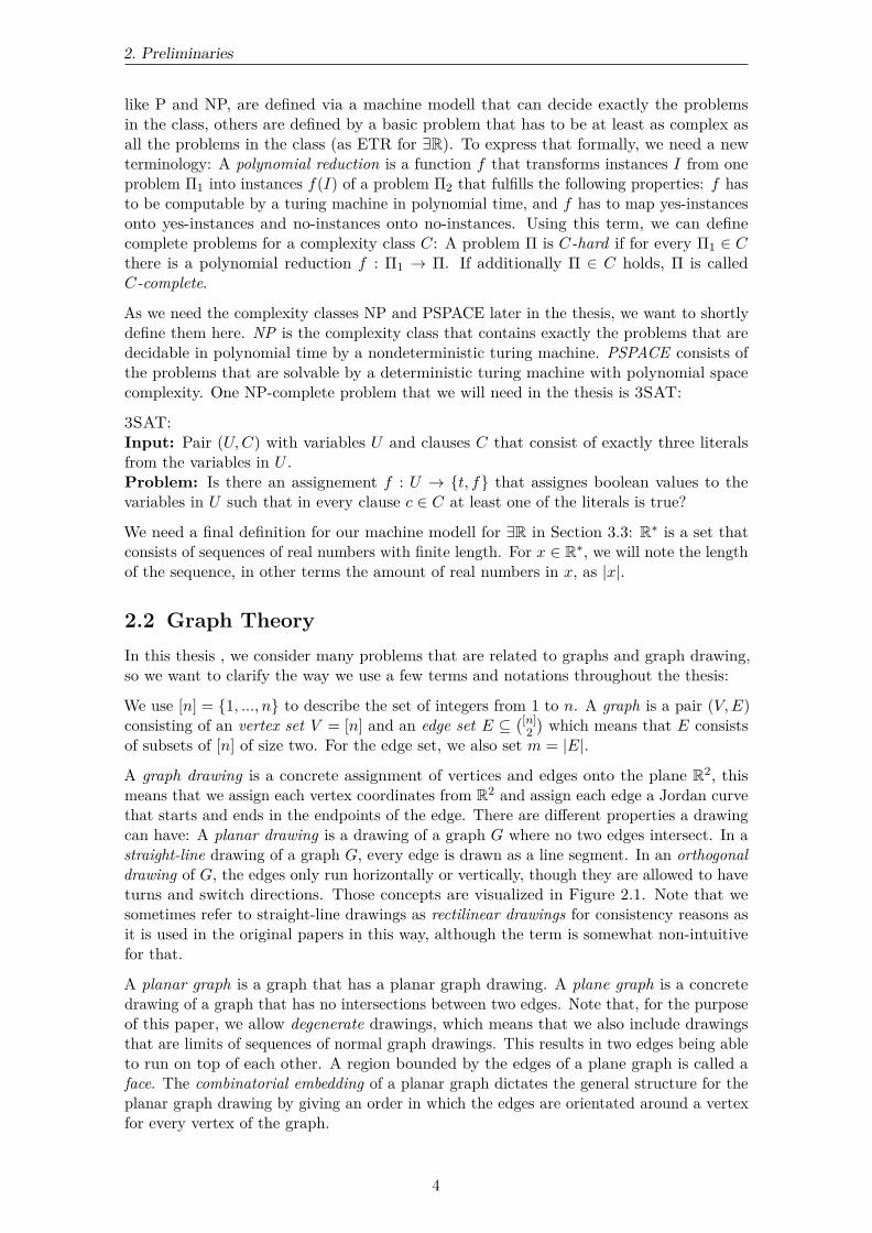
A graph drawing is a concrete assignment of vertices and edges onto the plane R2, thismeans that we assign each vertex coordinates from R2 and assign each edge a Jordan curvethat starts and ends in the endpoints of the edge. There are different properties a drawingcan have: A planar drawing is a drawing of a graph G where no two edges intersect. In astraight-line drawing of a graph G, every edge is drawn as a line segment. In an orthogonaldrawing of G, the edges only run horizontally or vertically, though they are allowed to haveturns and switch directions. Those concepts are visualized in Figure 2.1. Note that wesometimes refer to straight-line drawings as rectilinear drawings for consistency reasons asit is used in the original papers in this way, although the term is somewhat non-intuitivefor that.
A planar graph is a graph that has a planar graph drawing. A plane graph is a concretedrawing of a graph that has no intersections between two edges. Note that, for the purposeof this paper, we allow degenerate drawings, which means that we also include drawingsthat are limits of sequences of normal graph drawings. This results in two edges being ableto run on top of each other. A region bounded by the edges of a plane graph is called aface. The combinatorial embedding of a planar graph dictates the general structure for theplanar graph drawing by giving an order in which the edges are orientated around a vertexfor every vertex of the graph.
4
2.3. Algebra
Figure 2.1: A planar drawing, an orthogonal drawing, a straight-line drawing and a non-planar drawing of a graph G
As a final definition, we introduce the concept of an incidence graph G(φ) = (V (φ), E(φ))to an ETR formula φ. V (φ) includes a vertex vu for each variable u from φ, and a vertexvp for each equation or inequality p in φ. There are no edges between two variable verticesand no edges between two equation vertices in E(φ), and the edge vuvp is in E(φ) if andonly if the variable u is used in p.
2.3 AlgebraFinally, in Chapter 3, we mention the connection between the Existential Theory of theReals and its underlying algebraic relations. For that we need a few definitions:
A semialgebraic set S is a set of points in Rn that can be described via a quantifier-freeformula φ of polynomial equations and inequalities. Each member x ∈ S then has to bea solution of φ. If S can be defined by only conjunctions of polynomial equations andinequalities, S is called a basic semialgebraic set. If we additionally only allow equations, Sis called an algebraic set.
A real closed field is a field F with the same first order properties as the real numbers: Asentence φ of first order logic is feasible with variables from F if and only if it is feasiblewith variables from R.
To prepare for Mnëv’s Universality Theorem, which we deal with in Chapter 4, weadditionally need the concept of Rank-3 Orientated Matroids. As we do not work withthem in detail in the thesis, we do not give an exact definition here and just intuitivelyexplain the concept. A rank-3 oriented matroid is a combinatorial abstraction of a set Pof points in the plane that uses the order type (defines for three points in a plane if theyare collinear or form a left or a right turn) as a way to measure relations between threepoints. It can be expressed as a ternary predicate χ(p, q, r). This predicate has to fulfillthe chirotope axioms cyclic symmetry, antisymmetry and Grassmann-Plücker relations. Amore detailed explanation can be found here [CK13].
5

3. Complexity Class ∃R
First, we define our main problem ETR and the corresponding complexity class ∃R:
3.1 DefinitionThe Existential Theory of the Reals is the set of all true logic formulas from the existentialfirst order logic over real numbers. These formulas include real variables xi, which can beused in polynomial equations and inequalities with integer coefficients. The ExistentialTheory of the Reals then consists of all sentences of this structure that are feasible.This means that we can introduce all variables with existential quantifiers and compriseour definition of the Existential Theory of the Reals to all true formulas of the followingstructure: ∃x1, . . . , xn : p(x1, . . . , xn), with p being such a logical combination of polynomialequations and inequalities. Formally, we can define the corresponding decision problemETR in the following way:
ETR:Input: Formula ∃x1, . . . , xn : p(x1, . . . , xn) where p is a quantifier-free formula over thesignature 0, 1,+, ·, <,≤,= with connectives ∨,∧,¬.Problem: Are there real numbers x1, . . . , xn for which the formula p is true?
An example for such an instance of ETR can be a simple formula of the following structure:
φ ≡ ∃x, y, z ∈ R : (x2 + 3y = 1 ∨ x = z) ∧ z ≤ 0
This formula is feasible, e.g. with variables x = z = −1, y = 0, and therefore φ belongsto the Existential Theory of the Reals. Note that, while not technically allowed in thedefinition of ETR, we use multiple abbreviations such as writing x2 instead of x · x and3 instead of (1 + 1 + 1), which are obviously equivalent. We use these abbreviationsthroughout the thesis.
Note that solution sets of the Existential Theory of the Reals directly correspond to thealgebraic term semialgebraic set as their definitions are similar. This connection can behelpful when considering properties of semialgebraic sets that can be used in reductions inthis topic. Mnëv [Mnë88], Schaefer [Sch09] and McDiarmid and Müller [MM13] all usedthis approach for their reductions, as we mention again later in the thesis. We do not gointo detail for this direction though, as our thesis mainly looks at the reductions from ageometric viewpoint.
7
3. Complexity Class ∃R
With the help of the problem ETR, we can now define a complexity class that includesall problems that can be expressed (in a formula of polynomial length) in the ExistentialTheory of the Reals:
Definition 3.1 (∃R). The complexity class ∃R consists of the problems that can be reducedto the Existential Theory of the Reals (ETR) in polynomial time.
One can compare the relation of ∃R and ETR to the relation between NP and SAT. Thebiggest difference is that for SAT, NP-completeness was proven by Cook [Coo71] whilefor ETR, ∃R-completeness follows from the definition of ∃R. Still, both problems are thestarting point for every hardness proof in NP and ∃R respectively. Known problems thatare complete for ∃R generally are from topology, game theory, geometry or graph drawing.For this thesis, we focus on the graph drawing problems, for topology and game theory werefer to [SŠ17] and [BM16]. The complexity class was first proposed by Schaefer [Sch09],and then quickly adopted and expanded by other authors, notably Miltzow who, alongwith other colleagues, has designed reductions for multiple graph drawing problems whichwe explore later.
Note that, although the existential first order logic over real numbers is not expressable andcomputable by turing machines as the input is not finite, the input of the problem ETR(and thus of all problems in ∃R as they have to be transformable into ETR) is finite becauseonly integer coefficiants are allowed. This means that we can use the same definition forpolynomial transformations between problems in this context, although the solutions ofthe problems can contain real numbers.
We now classify our new complexity class into the hierarchy of known complexity classesand then discuss a theoretical equivalent machine modell to ∃R similar as turing machinesto P and NP. After that, we introduce multiple variants of ETR that are equivalent intheir complexity and will later be the foundation to show ∃R-completeness for multiplegeometrical and graph drawing problems.
3.2 ClassificationWhile there have been successful attempts to generalize ∃R and to build a more detailedhierarchy by adding more quantifiers by Dobbins et al. ([DKMR18]), similar to thepolynomial hierarchy, we focus on simply classifying ∃R itself. The result we get andexplain in the following sections is:
Theorem 3.2 ([Sch09], [Can88]). NP ⊆ ∃R ⊆ PSPACE
3.2.1 NP ⊆ ∃R
In this section, we prove that NP is a subset of ∃R. For that, it is sufficient to show that a3SAT instance can be polynomially reduced to an ETR-formula. 3SAT is NP-complete, soevery problem in NP can be polynomially reduced to 3SAT and then to ETR, thus everyproblem in NP is also in ∃R and NP ⊆ ∃R.
Note that is it unlikely that NP = ∃R holds as there are instances of many of the ∃R-complete problems that require irrational coordinates for displaying their solutions, thusthe solutions cannot be directly computed by turing machines. In Chapter 5, we explicitlygive such an instance for the problem DrawingOnSegments.
8
3.2. Classification
Lemma 3.3 ([Sch09]). NP ⊆ ∃R
Proof. We mainly follow the proof Schaefer gave in [Sch09], but modify it at a few pointsto make it easier to understand.
Let (U,C) be a 3SAT instance with variables U and C as the set of clauses. We constructan ETR-formula φ that is satisfiable if and only if (U,C) is satisfiable as well. First of all,for each 3SAT variable u ∈ U we introduce a real variable xu. For each of the real variablesxu also add the following formula: (xu = 1 ∨ xu = 0), all combined by conjunctions.Finally, let l be a literal in a clause c ∈ C. If l is not negated, use let bl = xl, if it is negated,then bl = (1− xl). For each c ∈ C with literals x, y, z add (bx + by + bz ≥ 1) to φ.
This reduction is polynomial because for each 3SAT variable and each clause there is aconstant part of φ, so the size of the formula is polynomial in the size of the 3SAT instance.If the 3SAT instance is satisfiable, an assignment of variables exists so that each clause issatisfied. For each 3SAT variable u that is true under the assignement choose xu = 1, foreach false variable xu = 0 for the real counterpart. Every clause is satisfied, so in each ofthe (bx + by + bz), one of the bi has to be 1 so each of these formulas are true. That meansthe whole formula is satisfied. On the other hand, if φ is satisfied, there is an assignementthat assigns each of the real variables xu either the value 0 or 1. One can construct anassignment of 3SAT variables by setting u true exactly when xu = 1, and false otherwise.Then, each of the clauses is satisfied because if there was a clause x ∨ y ∨ z that was notsatisfied, the formula bx + by + bz ≥ 1 would not be satisfied as well and thus φ would notbe true.
3.2.2 ∃R ⊆ PSPACE
For the other part of Theorem 3.2, we take a look at the development of algorithms thatsolve ETR throughout the later part of the 20th century. They develop from solving themore general first order logic over real numbers in exponential time and space to specificETR-algorithms that only need polynomial space. We then shortly mention more modernand efficient algorithms and implementations to solve ETR. The running time of thesealgorithms is dependant on four variables: the number of variables n, the number ofpolynomials m, the total degree of the polynomials d and the coefficient bit length L.
Lemma 3.4 ([Can88]). ∃R ⊆ PSPACE
Historically, there were multiple different algorithms that can be used to solve the decidabil-ity of ETR-formulas. The first algorithms solve a more general problem, the general firstorder logic of the reals (which corresponds to real closed fields in an algebraic sense). Theperson who first showed that this problem is decidable was Alfred Tarski in 1948 [Tar98]where he used a method called quantifier elimination to reduce a formula of the first orderlogic to a formula that does not contain quantifiers and its satisfiability does not change.However, this algorithm is not practical because its time complexity is non-elementary andcannot be bounded by any tower of exponentials.
In 1975, John Collins designed a new algorithm to solve the same problem, quantifierelimination in the real first order logic [Col75]. He used a new technique called CylindricalAlgebraic Decomposition (CAD) to vastly speed up the computation time. Althoughthe theoretical time complexity is double exponential, it is quite fast in practice and wasimplemented and improved multiple times since then, e.g. by Brown in the QEPCAD-Bsystem [Bro03].
9
3. Complexity Class ∃R
In 1987, Grigor’ev and Vorobjov designed an algorithm for solving ETR that reduced thecomplexity to L(md)n2 , although still needing an exponential amount of space [GVJ88].One year later, Canny developed an algorithm with polynomial space complexity forETR, thus proving that ∃R⊆ PSPACE [Can88]. From a complexity theory point of view,this result is important and has not been refined since. Renegar later improved Canny’salgorithm to run in L·log(L)·log(L)(md)O(n) while the space complexitiy stayed polynomial,thus preserving a polynomial runtime if the number of variables is fixed, a property Canny’salgorithm did not have [Ren88].
Although the algorithms of Grigorev and Renegar focus on a more specialized problemthan Collins and have a better theoretical runtime, they are dramatically slower on smallinputs as Hong discovered in 1991 [H+91]. While Collin’s algorithm can solve inputs withsmall parameters in seconds on modern computers, Renegar und Grigorev would needmore than a million years to calculate a solution even if every single parameter (number ofvariables, number of polynomials, total degree and coefficient bit length) is just 2. Becauseof that, these algorithms designed especially for ETR are mostly of theoretical value. Still,there have been attempts to at least use the new ideas for algorithms that perform in anacceptable manner for special cases of ETR [HRS93].
3.3 Machine ModelWe present a machine modell for ∃R similar to turing machines for P and NP. There havebeen attempts to conceptualize what machine modells for problems over real numberscould look like. The work we explore is from Blum, Shub and Smale and is called theBSS-machine [BSS+89]. While the BSS-machine itself corresponds to a wider field ofproblems, there are subclasses in the hierarchy of the BSS-machine that are achieved byremoving features from the machine, and one of these subclasses directly corresponds tothe Existential Theory of the Reals.
The BSS-machine is a register machine where it is assumed that real numbers can be saved,loaded and computed exactly in constant time and constant space (unlike reality where wewould need to approximate them and run into space and time problems as well as roundinginaccuracies. Formally, the BSS-machine was defined in the following way by Grädel:
Definition 3.5 (BSS-machine [Gra07]). A BSS-machine B over R is a register machinewithout an explicit working register. It consists of N instructions. The input x ∈ R∗ issaved in the first |x| registers. A configuration of B consists of 4 variables: the currentinstruction k ∈ [0, . . . , N ], the reading and writing registers r, w ∈ N and the current contentof the registers, z ∈ R∗. There are three types of instructions:
• Compute a rational function f(z) and save the result in the first register, andoptionally update the read and write registers to either the next one or the first one
• Branch if the first register has a non-negative content
• Copy the value of the read register to the write register
Similar to the definitions of P and NP with turing machines, we can define PR and NPR inour BSS-setting. For NPR we do that explicitly because we need the class later:
Definition 3.6 (NPR [Gra07]). A set L ⊆ R∗ is in NPR if there exists a nondeterministicBSS-machine B that decides L in polynomial time.
We do not go into detail how a nondeterministic BSS-machine B can be defined. Oneway to look at it is analogously to nondeterministic turing machines: B can guess real
10
3.4. Variants
numbers y ∈ R∗ before the computation starts, y then acts as a witness that helps provethe correctness of the input x (if x is correct).
The BSS-machine was designed for a much broader context than the Existential Theoryof the Reals, it can even be used for other rings than the ring of the real numbers. Wecan still find a subclass of this modell which corresponds to our problem, as Bürgisserand Cucker describe [BC06]. The subclass is denoted as BP (NP 0
R). The two restrictionscompared to the general class NPR are that there are no registers allowed (indicated bythe 0) and that the input has to be encoded as a string of 0 and 1 (indicated by the BP,short for boolean part). These restrictions narrow down the BSS-setting just enough thatwe land in our complexity class ∃R:
Theorem 3.7 ([BC06]). The class BP (NP 0R) of the BSS-machine modell directly corre-
sponds to the Existential Theory of the Reals.
For the proof, we need a variant of ETR called Feasibility,which we reuse later in thethesis. This variant restricts ETR-formulas to only consist of one polynomial that is testedon its equality to zero:
Feasibility:Input: ETR instance, of the form ∃x1, . . . , xn : g(x1, . . . , xn) = 0.Problem: Are there real numbers x1, . . . , xn for which the formula is true?
Proof outline (Theorem 3.7). The main idea of the proof is to show that the problemFeasibility is both complete for ∃R and for BP (NP 0
R). We show in the next section thatFeasibility is indeed complete for ∃R, although it restricts the structure of the formulasa lot. For now, we outline the proof by Bürgisser and Cucker [BC06] that Feasibility, orFeasibilityZ
R (meaning that we have a polynomial over R with integer coefficients, exactlyour setting) as it is denoted in their paper, is BP (NP 0
R)-complete. For that, they showthat the more general problem FeasibilityR where the coefficients can be real numbersas well is NPR-complete. This was in fact already shown by Blum et al. in their originalpaper [BSS+89] by reducing the FeasibilityR to polynomials with a maximal degree of 4and then proving NPR-completeness for that problem. Bürgisser and Cucker then outlinethat the reduction of an arbitrary problem in NPR to FeasibilityR directly leads to areduction in the BP (NP 0
R)-context to Feasibility, and consecutively, Feasibility isindeed complete in BP (NP 0
R).
With this equivalence, we get a new possibility to define ∃R, similar to how NP is canonicallydefined over nondeterministic turing machines. This topic has not yet been explored muchthough, and we are going to stop here as well as our main purpose of this thesis is toshow how geometrical ∃R-completeness proofs can be achieved. For that, we now lay thefoundation by giving multiple possible starting points for these reductions.
3.4 Variants
Now we take a look at different versions of ETR that will be our toolbox to prove ∃R-completeness for our different problems in the next chapters, for example Feasibility.All these variants restrict the way the formulas and variables are constructed to allow foreasier reductions.
11
3. Complexity Class ∃R
3.4.1 Feasibility and StrictIneq
The first variant we explore is StrictIneq which only allows strict inequalities. Althoughthese theories correspond to different algebraic constructs (as e.g. x2 = 2 cannot beexpressed without equations), the complexity classes one could define over them areidentical, as Marcus Schaefer proved in [SŠ17].
Theorem 3.8 ([SŠ17]). ETR, Feasibility and StrictIneq are polynomial-time equiva-lent.
Proof outline. One direction of the proof is easy, because every operation allowed inStrictIneq is also allowed in ETR, so every problem portrayable in StrictIneqistrivially portrayable in ETR. To prove the opposite direction, Schaefer uses Feasibilityof the previous section. He then proves that ETR reduces to Feasibility by using thatevery semi-algebraic set is a projection of an algebraic set, and proves that Feasibilityreduces to StrictIneq by using multiple distance observations for semi-algebraic sets totransform the equation g(x1, ..., xn) = 0 into a system of inequalities, thus showing thatETR can be reduced to Feasibility which then can be reduced to StrictIneq.
3.4.2 ETR-INV
While these variants already restrict ETR a lot, we go even further to ease our reductionseven more. We limit the logical operations to just conjunctions, as well as having onlyequations of specific types. The problem ETR-INV does exactly that:
ETR-INV
ETR-INV:Input: ETR instance where the equations and inequalities are all of one of the followingforms: x = 1, x + y = z or x · y = 1. Additionally, the only logical operations that areallowed are conjunctions.Problem: Are there real numbers x1, . . . , xn in [0.5, 2] for which the formula is true?
This problem was introduced by Abrahamsen et al. [AAM18] to show that the art galleryproblem1 is ∃R-complete and is the foundation of multiple similar reductions. Although itrestricts the rules of ETR a lot, it is still ∃R-complete:
Theorem 3.9 ([AAM18]). ETR-INV is ∃R-complete.
Proof outline. First, ETR-INV is obviously in ∃R as it is only a restriction of ETR andthus all allowed formulas in ETR-INV are allowed in ETR as well. For the ∃R-completeness,we do not go into detail how the proof is done but instead refer to two papers where theproof is done in detail: In [AAM18], Abrahamsen et al. prove the ∃R-completeness ofETR-INV to then use it as a basis to show ∃R-completeness for the art gallery problem.They start with Feasibility and then slowly transform the formula into fitting into theallowed operations. In [AM19], Abrahamsen and Miltzow refine the work already done bythem and others and give a more detailed and comprehensive proof by defining multipleother variants of ETR along the way.
1As a reminder: The art gallery problem asks if, for a simply polygon P , there is a set of points withinthe polygon G that guards the whole polygon, in other words, for every point p on the boundary of P ,there is a guard g ∈ G so that the line segment pg is completely in the interior of P .
12
3.4. Variants
X
X
Y
Y
X Y
Z
X ′ Y ′
X + Y = Z
X + Y ′ = Z X ′ + Y = Z
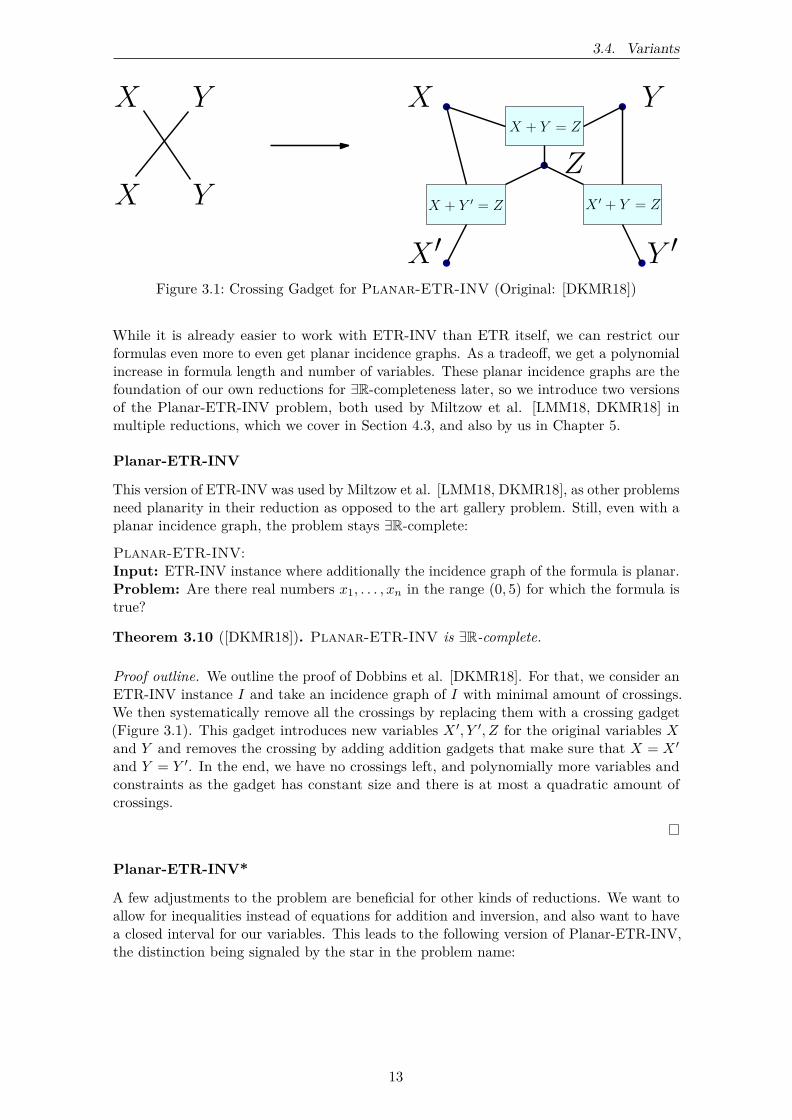
Figure 3.1: Crossing Gadget for Planar-ETR-INV (Original: [DKMR18])
While it is already easier to work with ETR-INV than ETR itself, we can restrict ourformulas even more to even get planar incidence graphs. As a tradeoff, we get a polynomialincrease in formula length and number of variables. These planar incidence graphs are thefoundation of our own reductions for ∃R-completeness later, so we introduce two versionsof the Planar-ETR-INV problem, both used by Miltzow et al. [LMM18, DKMR18] inmultiple reductions, which we cover in Section 4.3, and also by us in Chapter 5.
Planar-ETR-INV
This version of ETR-INV was used by Miltzow et al. [LMM18, DKMR18], as other problemsneed planarity in their reduction as opposed to the art gallery problem. Still, even with aplanar incidence graph, the problem stays ∃R-complete:
Planar-ETR-INV:Input: ETR-INV instance where additionally the incidence graph of the formula is planar.Problem: Are there real numbers x1, . . . , xn in the range (0, 5) for which the formula istrue?
Theorem 3.10 ([DKMR18]). Planar-ETR-INV is ∃R-complete.
Proof outline. We outline the proof of Dobbins et al. [DKMR18]. For that, we consider anETR-INV instance I and take an incidence graph of I with minimal amount of crossings.We then systematically remove all the crossings by replacing them with a crossing gadget(Figure 3.1). This gadget introduces new variables X ′, Y ′, Z for the original variables Xand Y and removes the crossing by adding addition gadgets that make sure that X = X ′
and Y = Y ′. In the end, we have no crossings left, and polynomially more variables andconstraints as the gadget has constant size and there is at most a quadratic amount ofcrossings.
Planar-ETR-INV*
A few adjustments to the problem are beneficial for other kinds of reductions. We want toallow for inequalities instead of equations for addition and inversion, and also want to havea closed interval for our variables. This leads to the following version of Planar-ETR-INV,the distinction being signaled by the star in the problem name:
13
3. Complexity Class ∃R
x
y
(a) Crossing betweenx and y
x
y
x′′
y′′
(b) High-level crossing gadget,orange dots are half-crossinggadget y
x
y
z x′
y′
x+ y ≤ z
z ≤ x′ + y
z ≤ x+ y′
(c) A half-crossing gadget
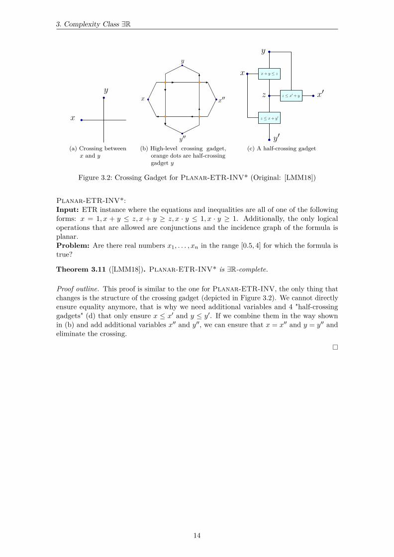
Figure 3.2: Crossing Gadget for Planar-ETR-INV* (Original: [LMM18])
Planar-ETR-INV*:Input: ETR instance where the equations and inequalities are all of one of the followingforms: x = 1, x + y ≤ z, x + y ≥ z, x · y ≤ 1, x · y ≥ 1. Additionally, the only logicaloperations that are allowed are conjunctions and the incidence graph of the formula isplanar.Problem: Are there real numbers x1, . . . , xn in the range [0.5, 4] for which the formula istrue?
Theorem 3.11 ([LMM18]). Planar-ETR-INV* is ∃R-complete.
Proof outline. This proof is similar to the one for Planar-ETR-INV, the only thing thatchanges is the structure of the crossing gadget (depicted in Figure 3.2). We cannot directlyensure equality anymore, that is why we need additional variables and 4 "half-crossinggadgets" (d) that only ensure x ≤ x′ and y ≤ y′. If we combine them in the way shownin (b) and add additional variables x′′ and y′′, we can ensure that x = x′′ and y = y′′ andeliminate the crossing.
14
4. Existing Problems and Reductions
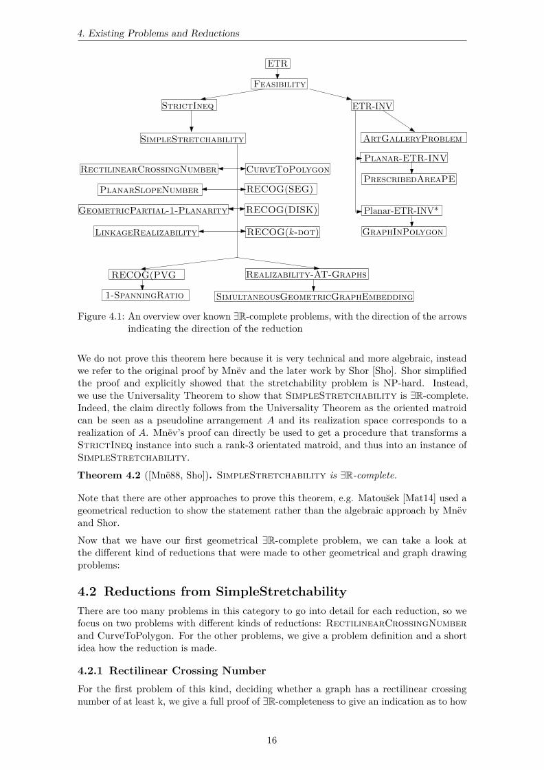
After learning about the complexity class and the different variants of ETR, we now givean overview over the problems that are already known to be ∃R-complete and categorizethe corresponding reductions. We focus on geometrical graph problems, but there are othercategories of problems that are known to be ∃R-complete, too, like topological problems orproblems belonging to game theory. All these reductions are from one of two problems:SimpleStretchability, which we cover in the next section, and ETR-INV (or its planarvariants), which we already introduced in the last chapter. Figure 4.1 gives an overviewover the reductions we look at in the following sections. We start with the proof by Mnëvthat SimpleStretchaility is ∃R-complete, and then generalize the reductions from thetwo basic problems.
4.1 Simple Stretchability of Pseudolines
The first problem to be proven ∃R-complete was SimpleStretchability. For that, wefirst need a few definitions: A pseudoline is a simple curve in the plane. A pseudolinearrangement A is a set of pseudolines that is situated in the plane such that pairs ofpseudolines cross each other exactly once. A is called simple if in each intersection nomore than two pseudolines cross. Two pseudoline arrangements A and B are isomorphicif there exists a homeomorphism (continous bijective function with a continous reversefunction) of the plane that maps A onto B. A realization of a pseudoline arrangement A isan arrangement of straight lines that is isomorphic to A. With these terms, we can definethe problem:
SimpleStretchability:Input: Simple arrangement A of pseudolines.Problem: Does an arrangement of line segments exist that is isomorphic to A?
The proof of the ∃R-completeness directly follows from Mnëv’s Universality Theorem, whichcovers the reduction from StrictIneq to SimpleStretchability, but in a differentcontext. We do not explain the concept of stable equivalence as it would need much morework and is not detrimental to our thesis, just note that it is a very strong statement thatexpresses much more than the reduction.
Theorem 4.1 (Universality Theorem [Mnë88]). Every semialgebraic set is stably equivalentto the realization space of a rank-3 oriented matroid.
15
4. Existing Problems and Reductions
ETR
Feasibility
StrictIneq ETR-INV
SimpleStretchability ArtGalleryProblem
RectilinearCrossingNumber
RECOG(SEG)
CurveToPolygonPlanar-ETR-INV
PrescribedAreaPE
Planar-ETR-INV*
GraphInPolygon
RECOG(PVG
PlanarSlopeNumber
GeometricPartial-1-Planarity
1-SpanningRatio SimultaneousGeometricGraphEmbedding
Realizability-AT-Graphs
RECOG(DISK)
RECOG(k-dot)LinkageRealizability
Figure 4.1: An overview over known ∃R-complete problems, with the direction of the arrowsindicating the direction of the reduction
We do not prove this theorem here because it is very technical and more algebraic, insteadwe refer to the original proof by Mnëv and the later work by Shor [Sho]. Shor simplifiedthe proof and explicitly showed that the stretchability problem is NP-hard. Instead,we use the Universality Theorem to show that SimpleStretchability is ∃R-complete.Indeed, the claim directly follows from the Universality Theorem as the oriented matroidcan be seen as a pseudoline arrangement A and its realization space corresponds to arealization of A. Mnëv’s proof can directly be used to get a procedure that transforms aStrictIneq instance into such a rank-3 orientated matroid, and thus into an instance ofSimpleStretchability.
Theorem 4.2 ([Mnë88, Sho]). SimpleStretchability is ∃R-complete.
Note that there are other approaches to prove this theorem, e.g. Matousek [Mat14] used ageometrical reduction to show the statement rather than the algebraic approach by Mnëvand Shor.
Now that we have our first geometrical ∃R-complete problem, we can take a look atthe different kind of reductions that were made to other geometrical and graph drawingproblems:
4.2 Reductions from SimpleStretchabilityThere are too many problems in this category to go into detail for each reduction, so wefocus on two problems with different kinds of reductions: RectilinearCrossingNumberand CurveToPolygon. For the other problems, we give a problem definition and a shortidea how the reduction is made.
4.2.1 Rectilinear Crossing NumberFor the first problem of this kind, deciding whether a graph has a rectilinear crossingnumber of at least k, we give a full proof of ∃R-completeness to give an indication as to how
16
4.2. Reductions from SimpleStretchability
such a proof looks like. The rectilinear crossing number of a graph G, denoted as lin-cr(G),is the minimal number of crossings a straight-line drawing of G can have. The decisionproblem takes an integer k and asks for an input graph G if lin-cr(G) ≤ k. This problem is∃R-complete even when G is restricted to be cubic, that means that every vertex in G hasa degree of three.
RectilinearCrossingNumber:Input: Cubic graph G, integer k.Problem: Is there a straight-line drawing of G with at most k crossings?
Theorem 4.3 ([Bie91, Sch09]). RectilinearCrossingNumber is ∃R-complete.
Proof. The proof of such a statement is done in two parts: First we show that the problemis in ∃R by giving an ETR-formula that is polynomial in size in the input size and isequivalent to the problem, and then we show that the problem is ∃R-hard by reducingETR to our problem. For RectilinearCrossingNumber, Schaefer proves that theproblem is in ∃R [Sch09] while Bienstock gives a reduction from SimpleStretchabilityto RectilinearCrossingNumber [Bie91].
RectilinearCrossingNumber is in ∃R
We need a few preliminaries to comprehend Schaefer’s proof: Let G = (V,E) be theinput graph. We assume that V = [n] and E ⊆
([n]2). We assume that the edges of G
are orientated in an arbitrary way such that we have a clearly defined head and tail foreach edge. With these orientations, we define functions h, t : E → V that return theendpoints of an edge e. The formula is build by having a pair of variables (xi, yi) for eachvertex encoding the position of the vertex in a planar drawing of G and then checking theproperties of the problem for that drawing.
Schaefer’s general idea for the formula is to allow at most k edges to cross by assigningadditional variables zei,ej to each pair of edges (ei, ej) and to ensure that at most k of thesezei,ej are greater than 0 which indicates that the pair of edges is allowed to cross. He alsoensures that if zei,ej is not greater than 0, then the corresponding edges do not intersect.Note that we only need to check each pair of edges once, and that the same edge does notcross itself, so we only need the additional zei,ej for i < j.
In detail, he needs three predicates for that. The first predicate atmostk(ze1,e2 , ..., zem−1,em)checks if at most k of the variables are greater than zero. The predicatecollinear(x1, y1, x2, y2, x3, y3) ensures that the three points (x1, y1), (x2, y2), (x3, y3) are notcollinear (do not lie on a line), and the final predicate cross(x1, y1, x2, y2, x
′1, y′1, x′2, y′2) en-
sures that the corresponding line segments with endpoints (xi, yi) and (x′i, y′i) respectivelydo not intersect.
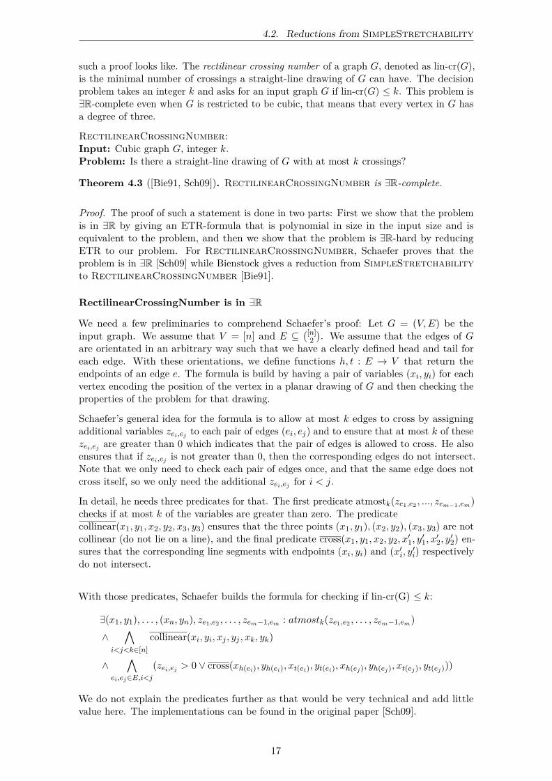
With those predicates, Schaefer builds the formula for checking if lin-cr(G) ≤ k:
∃(x1, y1), . . . , (xn, yn), ze1,e2 , . . . , zem−1,em : atmostk(ze1,e2 , . . . , zem−1,em)∧
∧i<j<k∈[n]
collinear(xi, yi, xj , yj , xk, yk)
∧∧
ei,ej∈E,i<j
(zei,ej > 0 ∨ cross(xh(ei), yh(ei), xt(ei), yt(ei), xh(ej), yh(ej), xt(ej), yt(ej)))
We do not explain the predicates further as that would be very technical and add littlevalue here. The implementations can be found in the original paper [Sch09].
17
4. Existing Problems and Reductions
Rectilinear Crossing Number is ∃R-hard
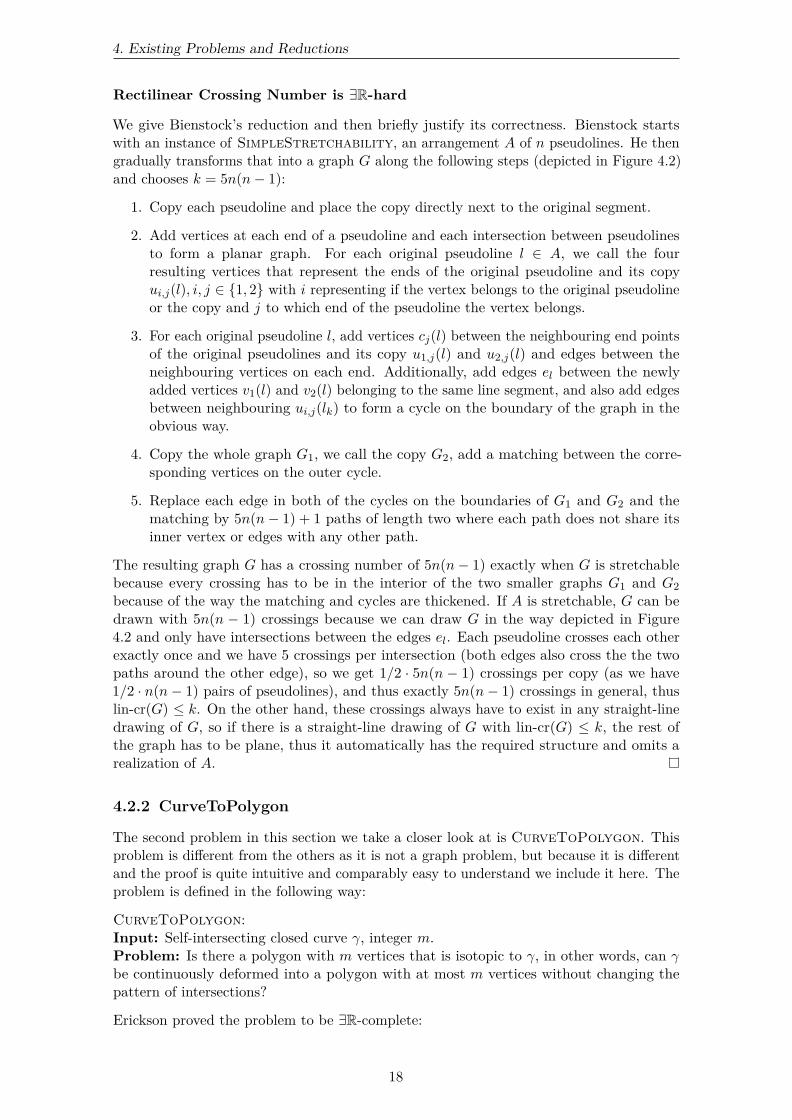
We give Bienstock’s reduction and then briefly justify its correctness. Bienstock startswith an instance of SimpleStretchability, an arrangement A of n pseudolines. He thengradually transforms that into a graph G along the following steps (depicted in Figure 4.2)and chooses k = 5n(n− 1):
1. Copy each pseudoline and place the copy directly next to the original segment.
2. Add vertices at each end of a pseudoline and each intersection between pseudolinesto form a planar graph. For each original pseudoline l ∈ A, we call the fourresulting vertices that represent the ends of the original pseudoline and its copyui,j(l), i, j ∈ 1, 2 with i representing if the vertex belongs to the original pseudolineor the copy and j to which end of the pseudoline the vertex belongs.
3. For each original pseudoline l, add vertices cj(l) between the neighbouring end pointsof the original pseudolines and its copy u1,j(l) and u2,j(l) and edges between theneighbouring vertices on each end. Additionally, add edges el between the newlyadded vertices v1(l) and v2(l) belonging to the same line segment, and also add edgesbetween neighbouring ui,j(lk) to form a cycle on the boundary of the graph in theobvious way.
4. Copy the whole graph G1, we call the copy G2, add a matching between the corre-sponding vertices on the outer cycle.
5. Replace each edge in both of the cycles on the boundaries of G1 and G2 and thematching by 5n(n− 1) + 1 paths of length two where each path does not share itsinner vertex or edges with any other path.
The resulting graph G has a crossing number of 5n(n− 1) exactly when G is stretchablebecause every crossing has to be in the interior of the two smaller graphs G1 and G2because of the way the matching and cycles are thickened. If A is stretchable, G can bedrawn with 5n(n − 1) crossings because we can draw G in the way depicted in Figure4.2 and only have intersections between the edges el. Each pseudoline crosses each otherexactly once and we have 5 crossings per intersection (both edges also cross the the twopaths around the other edge), so we get 1/2 · 5n(n − 1) crossings per copy (as we have1/2 · n(n− 1) pairs of pseudolines), and thus exactly 5n(n− 1) crossings in general, thuslin-cr(G) ≤ k. On the other hand, these crossings always have to exist in any straight-linedrawing of G, so if there is a straight-line drawing of G with lin-cr(G) ≤ k, the rest ofthe graph has to be plane, thus it automatically has the required structure and omits arealization of A.
4.2.2 CurveToPolygon
The second problem in this section we take a closer look at is CurveToPolygon. Thisproblem is different from the others as it is not a graph problem, but because it is differentand the proof is quite intuitive and comparably easy to understand we include it here. Theproblem is defined in the following way:
CurveToPolygon:Input: Self-intersecting closed curve γ, integer m.Problem: Is there a polygon with m vertices that is isotopic to γ, in other words, can γbe continuously deformed into a polygon with at most m vertices without changing thepattern of intersections?
Erickson proved the problem to be ∃R-complete:
18
4.2. Reductions from SimpleStretchability
Figure 4.2: The steps of the reduction for RectilinearCrossingNumber (Source:[Bie91])
19
4. Existing Problems and Reductions
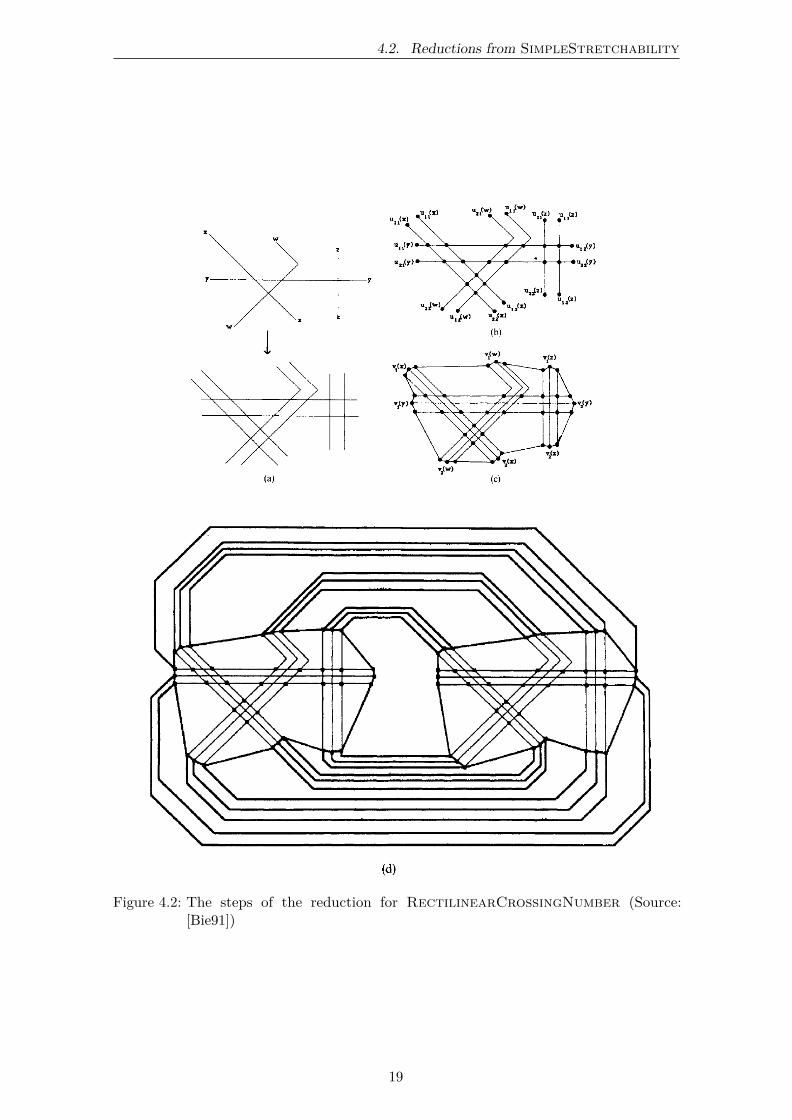
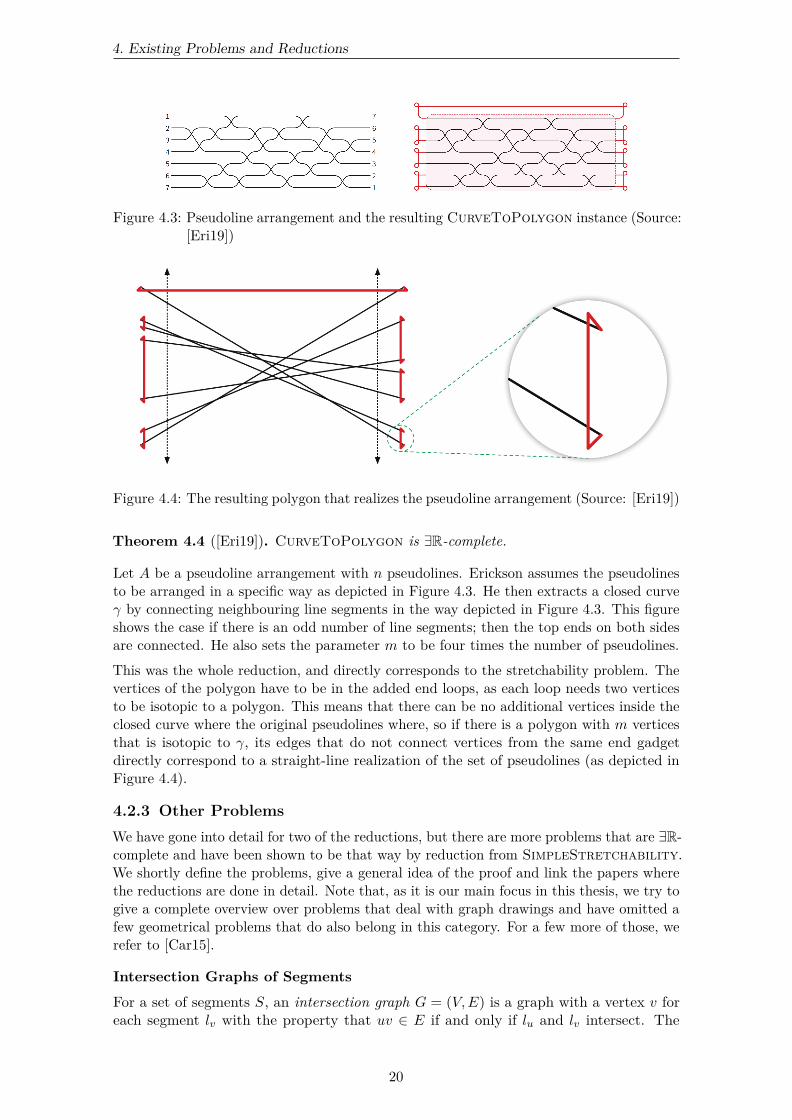
Figure 4.3: Pseudoline arrangement and the resulting CurveToPolygon instance (Source:[Eri19])
Figure 4.4: The resulting polygon that realizes the pseudoline arrangement (Source: [Eri19])
Theorem 4.4 ([Eri19]). CurveToPolygon is ∃R-complete.
Let A be a pseudoline arrangement with n pseudolines. Erickson assumes the pseudolinesto be arranged in a specific way as depicted in Figure 4.3. He then extracts a closed curveγ by connecting neighbouring line segments in the way depicted in Figure 4.3. This figureshows the case if there is an odd number of line segments; then the top ends on both sidesare connected. He also sets the parameter m to be four times the number of pseudolines.
This was the whole reduction, and directly corresponds to the stretchability problem. Thevertices of the polygon have to be in the added end loops, as each loop needs two verticesto be isotopic to a polygon. This means that there can be no additional vertices inside theclosed curve where the original pseudolines where, so if there is a polygon with m verticesthat is isotopic to γ, its edges that do not connect vertices from the same end gadgetdirectly correspond to a straight-line realization of the set of pseudolines (as depicted inFigure 4.4).
4.2.3 Other ProblemsWe have gone into detail for two of the reductions, but there are more problems that are ∃R-complete and have been shown to be that way by reduction from SimpleStretchability.We shortly define the problems, give a general idea of the proof and link the papers wherethe reductions are done in detail. Note that, as it is our main focus in this thesis, we try togive a complete overview over problems that deal with graph drawings and have omitted afew geometrical problems that do also belong in this category. For a few more of those, werefer to [Car15].
Intersection Graphs of Segments
For a set of segments S, an intersection graph G = (V,E) is a graph with a vertex v foreach segment lv with the property that uv ∈ E if and only if lu and lv intersect. The
20
4.2. Reductions from SimpleStretchability
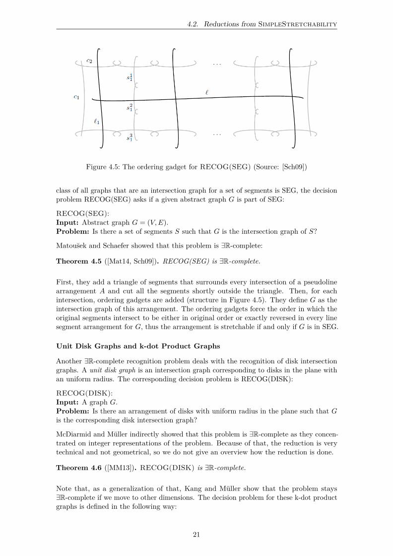
Figure 4.5: The ordering gadget for RECOG(SEG) (Source: [Sch09])
class of all graphs that are an intersection graph for a set of segments is SEG, the decisionproblem RECOG(SEG) asks if a given abstract graph G is part of SEG:
RECOG(SEG):Input: Abstract graph G = (V,E).Problem: Is there a set of segments S such that G is the intersection graph of S?
Matousek and Schaefer showed that this problem is ∃R-complete:
Theorem 4.5 ([Mat14, Sch09]). RECOG(SEG) is ∃R-complete.
First, they add a triangle of segments that surrounds every intersection of a pseudolinearrangement A and cut all the segments shortly outside the triangle. Then, for eachintersection, ordering gadgets are added (structure in Figure 4.5). They define G as theintersection graph of this arrangement. The ordering gadgets force the order in which theoriginal segments intersect to be either in original order or exactly reversed in every linesegment arrangement for G, thus the arrangement is stretchable if and only if G is in SEG.
Unit Disk Graphs and k-dot Product Graphs
Another ∃R-complete recognition problem deals with the recognition of disk intersectiongraphs. A unit disk graph is an intersection graph corresponding to disks in the plane withan uniform radius. The corresponding decision problem is RECOG(DISK):
RECOG(DISK):Input: A graph G.Problem: Is there an arrangement of disks with uniform radius in the plane such that Gis the corresponding disk intersection graph?
McDiarmid and Müller indirectly showed that this problem is ∃R-complete as they concen-trated on integer representations of the problem. Because of that, the reduction is verytechnical and not geometrical, so we do not give an overview how the reduction is done.
Theorem 4.6 ([MM13]). RECOG(DISK) is ∃R-complete.
Note that, as a generalization of that, Kang and Müller show that the problem stays∃R-complete if we move to other dimensions. The decision problem for these k-dot productgraphs is defined in the following way:
21
4. Existing Problems and Reductions
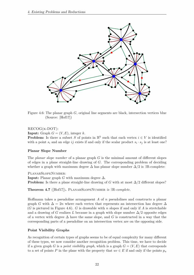
Figure 4.6: The planar graph G, original line segments are black, intersection vertices blue(Source: [Hof17])
RECOG(k-DOT):Input: Graph G = (V,E), integer k.Problem: Is there a subset S of points in Rk such that each vertex i ∈ V is identifiedwith a point si and an edge ij exists if and only if the scalar product si · sj is at least one?
Planar Slope Number
The planar slope number of a planar graph G is the minimal amount of different slopesof edges in a plane straight-line drawing of G. The corresponding problem of decidingwhether a graph with maximum degree ∆ has planar slope number ∆/2 is ∃R-complete:
PlanarSlopeNumber:Input: Planar graph G with maximum degree ∆.Problem: Is there a plane straight-line drawing of G with at most ∆/2 different slopes?
Theorem 4.7 ([Hof17]). PlanarSlopeNumber is ∃R-complete.
Hoffmann takes a pseudoline arrangement A of n pseudolines and constructs a planargraph G with ∆ = 2n where each vertex that represents an intersection has degree ∆(G is pictured in Figure 4.6). G is drawable with n slopes if and only if A is stretchableand a drawing of G realizes L because in a graph with slope number ∆/2 opposite edgesof a vertex with degree ∆ have the same slope, and G is constructed in a way that thecorresponding parts of a pseudoline on an intersection vertex are on the opposing side.
Point Visibility Graphs
As recognition of certain types of graphs seems to be of equal complexity for many differentof these types, we now consider another recognition problem. This time, we have to decideif a given graph G is a point visibility graph, which is a graph G = (V,E) that correspondsto a set of points P in the plane with the property that uv ∈ E if and only if the points pu
22
4.2. Reductions from SimpleStretchability
and pv see each other, which means that there is no other point p ∈ P on the line segmentbetween pu and pv. Cardinal and Hoffman show that this decision problem is ∃R-complete:RECOG(PVG):Input: Graph G = (V,E).Problem: Is G a point visibility graph, in other words, does a set P with |P | = n ofpoints in the plane and a bijective function between P and V exist so that uv ∈ E if andonly if pu and pv see each other?Theorem 4.8 ([CH17]). RECOG(PVG) is ∃R-complete.
We want to highlight that Cardinal and Hoffman use a different method to prove ∃R-completeness for this problem as they followed the idea of Mnëv and showed that a semial-gebraic set is stably equivalent to the realization space of an instance of RECOG(PVG).There is a direct relation between point visibility graphs and the spanning ratio of graphs.The spanning ratio of a graph G = (V,E) is the minimal k so that, for each pair u, v ∈ Vthe edge distance on the shortest path between u and v is at most k · ||uv||. As Aichholzeret al. showed [ABB+20], the answer to the question if a given graph has a spanning ratioof one is yes if and only if the graph is a point visibility graph. Thus, the following problemis also ∃R-complete:1-SpanningRatio:Input: Graph G = (V,E).Problem: Can G be drawn as a proper straight-line drawing with spanning ratio 1?
Realization of AT graphs and Simultaneous Geometric EmbeddingAn abstract topological graph is a pair AT = (G,R) with R being a set of pairs of edgesfrom G. R expresses which edges of G are allowed to cross in a drawing of G. A weakrealization of AT is a drawing of G where only the edge pairs in R cross, if all of themcross in the drawing, it is just called a realization. For a given AT-graph, deciding whetherit is (weak) realizable with a straight-line drawing is ∃R-complete, as shown by Kyncl. Weare going to focus on the weak version of the problem as it leads to another ∃R-completeproblem:WeakRectilinearRealizability:Input: Abstract topological graph T = (G,R).Problem: Does a straight-line drawing of G exist where only edge pairs from R cross?Theorem 4.9 ([Kyn11]). WeakRectilinearRealizability is ∃R-complete.
Kyncl constructs an AT-graph T from a pseudoline arrangement A with n pseudolinesby placing a circle around all the intersections in A. He then defines T as a cycle of6n vertices with n chords corresponding to the pseudolines and 2n additional paths thatconnect certain vertices of the cycle and have length n − 1. Two types of crossings areallowed: chords can cross each other and the edge pj of a path j can cross the chord cj . Tis realizable if and only if A is stretchable as the chords directly correspond to the stretchedpseudolines.Cardinal then used that problem to show ∃R-completeness for another graph drawingproblem, Simultaneous Geometric Embedding (or k-SGE) as it is equivalent [Car15]. Notethat the reduction only works when k is for some constant c at least in Ω(nc) for the size nof the original instance.k-SGE:Input: k Graphs G1 = (V,E1), . . . Gk = (V,Ek) with a shared vertex set V .Problem: Does a set of coordinates P ⊂ R2 and a bijection π : V → P exist such thatevery induced drawing of any Gi is planar?
23
4. Existing Problems and Reductions
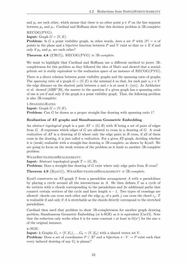
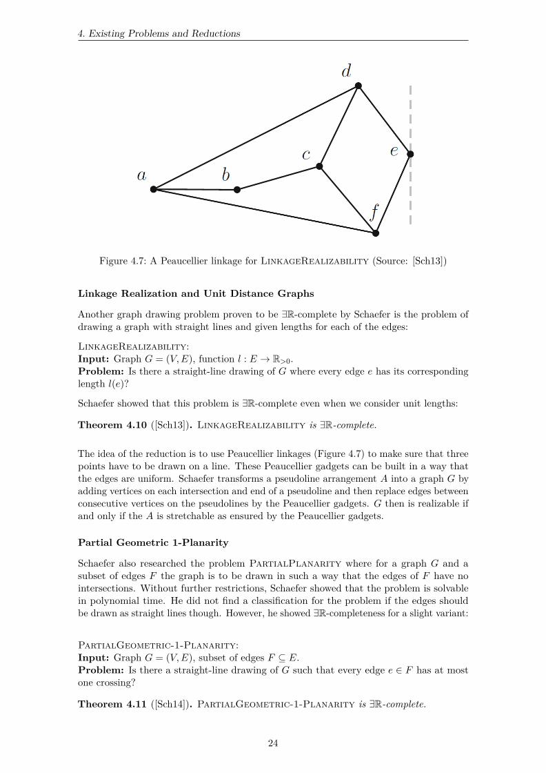
Figure 4.7: A Peaucellier linkage for LinkageRealizability (Source: [Sch13])
Linkage Realization and Unit Distance Graphs
Another graph drawing problem proven to be ∃R-complete by Schaefer is the problem ofdrawing a graph with straight lines and given lengths for each of the edges:
LinkageRealizability:Input: Graph G = (V,E), function l : E → R>0.Problem: Is there a straight-line drawing of G where every edge e has its correspondinglength l(e)?
Schaefer showed that this problem is ∃R-complete even when we consider unit lengths:
Theorem 4.10 ([Sch13]). LinkageRealizability is ∃R-complete.
The idea of the reduction is to use Peaucellier linkages (Figure 4.7) to make sure that threepoints have to be drawn on a line. These Peaucellier gadgets can be built in a way thatthe edges are uniform. Schaefer transforms a pseudoline arrangement A into a graph G byadding vertices on each intersection and end of a pseudoline and then replace edges betweenconsecutive vertices on the pseudolines by the Peaucellier gadgets. G then is realizable ifand only if the A is stretchable as ensured by the Peaucellier gadgets.
Partial Geometric 1-Planarity
Schaefer also researched the problem PartialPlanarity where for a graph G and asubset of edges F the graph is to be drawn in such a way that the edges of F have nointersections. Without further restrictions, Schaefer showed that the problem is solvablein polynomial time. He did not find a classification for the problem if the edges shouldbe drawn as straight lines though. However, he showed ∃R-completeness for a slight variant:
PartialGeometric-1-Planarity:Input: Graph G = (V,E), subset of edges F ⊆ E.Problem: Is there a straight-line drawing of G such that every edge e ∈ F has at mostone crossing?
Theorem 4.11 ([Sch14]). PartialGeometric-1-Planarity is ∃R-complete.
24
4.3. Reductions from ETR-INV and its Variants
For the reduction, Schaefer surrounds the intersections of the pseudoline arrangement Awith a parabola R. He then constructs a graph from that by playing vertices on eachintersection of a line segment with the boundary, on each inner face of the resultingarrangement and an additional one below the parabola. He adds edges corresponding tothe dual graph of the pseudoline arrangement and K6 gadgets to ensure that a drawing ofthe graph leads to a realization of A.
4.3 Reductions from ETR-INV and its VariantsOverall, as we mentioned before, the reductions from SimpleStretchability differ verymuch and depend on the right idea for the specific problem. Now, we consider the secondapproach for showing ∃R-completeness, reductions from ETR-INV, where we find a structurein the reductions that is much easier to replicate than the SimpleStretchability proofs.As a reminder, here is the general ETR-INV problem:
ETR-INV:Input: ETR instance where the variables are equations and inequalities are all of one ofthe following forms: x = 1, x+ y = z, x · y = 1. Additionally, the only logical operationsthat are allowed are conjunctions.Problem: Are there real numbers in [0.5, 2] for which the formula is true?
The reductions from ETR-INV, as opposed to the ones in the previous section, all followthe same blueprint: We build specific structures in the setting of our problem to encodevariables and to implement the different kinds of allowed formulas. We also need a way totransfer values of variables. We give three examples where this general idea is implementedin different ways. As a side note, Abrahamsen et al. [AMS20] modified this approach toalso work for geometrical packing problems instead of graph drawing problems.
4.3.1 Drawing a Graph in a Polygonal Region
The problem we mainly focus on is GraphInPolygon. We reuse and slightly modify mostof the gadgets later in Chapter 5 for our own proof. The problem is the following:
GraphInPolygon:Input: Planar graph G = (V,E), polygonal region R, subset of V with fixed positions onthe border of R.Problem: Is there a planar straight-line drawing of G where the fixed vertices are drawnon their assigned positions?
Lubiw et al. [LMM18] show that this problem is complete in ∃R, using the blueprint forreductions from ETR-INV problems:
Theorem 4.12 ([LMM18]). GraphInPolygon is ∃R-complete.
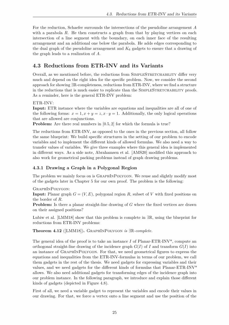
The general idea of the proof is to take an instance I of Planar-ETR-INV*, compute anorthogonal straight-line drawing of the incidence graph G(I) of I and transform G(I) intoan instance of GraphInPolygon. For that, we need geometrical figures to express theequations and inequalities from the ETR-INV-formulas in terms of our problem, we callthem gadgets in the rest of the thesis. We need gadgets for expressing variables and theirvalues, and we need gadgets for the different kinds of formulas that Planar-ETR-INV*allows. We also need additional gadgets for transforming edges of the incidence graph intoour problem instance. In the following paragraph, we introduce and explain those differentkinds of gadgets (depicted in Figure 4.8).
First of all, we need a variable gadget to represent the variables and encode their values inour drawing. For that, we force a vertex onto a line segment and use the position of the
25
4. Existing Problems and Reductions
(a) Variable gadget (b) Copy gadget (c) Split gadget
(d) Turn gadget (e) Addition gadget (f) Inversion gadget
Figure 4.8: The gadgets for GraphInPolygon (Source: [LMM18])
vertex on the line segment to represent the value of the variable. How that is done can beseen in Figure 4.8 a): The fixed vertex a and the two peaks of the polygon ensure that thevertex p has to be at the same height as a, and the vertex b forces v to be on the right sideof p. On the other side of the gadget, there is a mirrored construction that forces v to alsobe to the left of s, thus v has to be situated on the line segment ps.
We can divide the other gadgets into two categories: Formula gadgets that implement thedifferent operations allowed in Planar-ETR-INV* formulas and transport gadgets that weuse to replace the edges in the incidence graph to carry values of variables through thedrawing. We have three different transport gadgets. The copy gadget just copies the valueof a variable through space and replaces a straight-line part of an edge of the incidencegraph. The turn gadget implements rotations of an edge of 90 degrees. The splitter gadgetis there to transfer the value of a variable to different parts of the incidence graph if avariable vertex has a degree of more than one. Additionally, we have addition gadgets thatensure that a variable gadget z has value at most x+ y (or at least x+ y respectively) andinversion gadgets who ensure that, for two variable gadgets x and y, x · y ≤ 1 or x · y ≥ 1holds respectively. The gadgets are depicted in Figure 4.8. We explain how and why theywork in Chapter 5.
The final step now is to transform the planar incidence graph into an instance of GraphIn-Polygon. For that, we replace variable vertices with variable gadgets, formula verticeswith the corresponding gadgets and edges with copy and turn segments. We again go intodetail in Chapter 5 why this transformation is correct and always possible.
4.3.2 Art Gallery ProblemThe art gallery problem is the first problem that was shown to be ∃R-complete via reductionfrom ETR-INV. Abrahamsen et. al [AAM18] explicitly designed the ETR-INV problem torestrict the possible equations in the ETR formula to be better expressable with specificgadgets. The gadgets are built by using properties of the art gallery problem, which isdefined in the following way:
26
4.3. Reductions from ETR-INV and its Variants
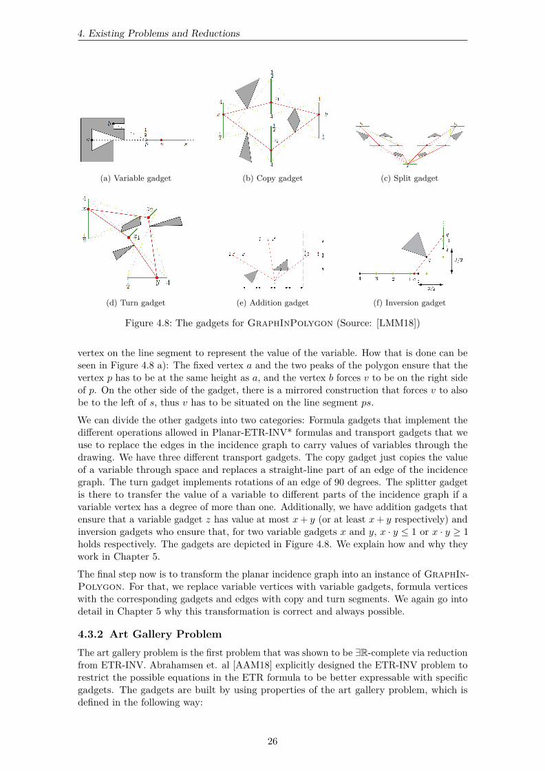
Figure 4.9: High-level polygon of the art gallery problem (Source: [AAM18])
ArtGalleryProblem:Input: Simple polygon P with corners at rational coordinates, integer k.Problem: Is there a set G of k guards (points in P ) that guards all of P , so that for eachp ∈ P there is a g ∈ G such that the line segment pg is completely in the interior of P?
Theorem 4.13 ([AAM18]). The art gallery problem is ∃R-complete.
Lubiw et al. base the reduction on the general ETR-INV problem. They again constructgadgets for each type of equation in ETR-INV, but do not need the planar incidence graphthat is the base of the previous reduction as the values of the variables are transmitted tothe gadgets without additional constructions.
The high level sketch of the polygon can be seen in Figure 4.9. On the bottom, thereare the guard segments which represent the variables of the formula. The gadgets are onthe left and right side, with corridors at the beginning copying the values of the guardsegments into the segments. The idea of the gadgets is that only specific points of theguard segments can see the entire gadget, and thus, to have an optimal set of guards, thesepoints have to be included and the values of the variables can be manipulated in this way.For more details we refer to the original paper. For better understanding how the polygoncan be used to manipulate values of variables, we discuss the guard segments a bit more.
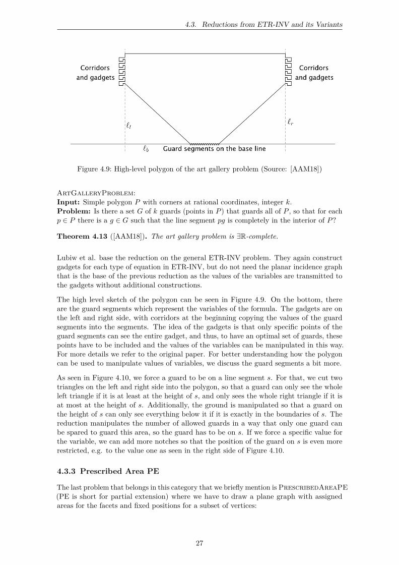
As seen in Figure 4.10, we force a guard to be on a line segment s. For that, we cut twotriangles on the left and right side into the polygon, so that a guard can only see the wholeleft triangle if it is at least at the height of s, and only sees the whole right triangle if it isat most at the height of s. Additionally, the ground is manipulated so that a guard onthe height of s can only see everything below it if it is exactly in the boundaries of s. Thereduction manipulates the number of allowed guards in a way that only one guard canbe spared to guard this area, so the guard has to be on s. If we force a specific value forthe variable, we can add more notches so that the position of the guard on s is even morerestricted, e.g. to the value one as seen in the right side of Figure 4.10.
4.3.3 Prescribed Area PE
The last problem that belongs in this category that we briefly mention is PrescribedAreaPE(PE is short for partial extension) where we have to draw a plane graph with assignedareas for the facets and fixed positions for a subset of vertices:
27
4. Existing Problems and Reductions
Figure 4.10: Guard segments for the art gallery problem (Source: [AAM18])
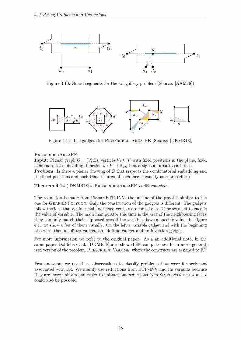
Figure 4.11: The gadgets for Prescribed Area PE (Source: [DKMR18])
PrescribedAreaPE:Input: Planar graph G = (V,E), vertices Vf ⊆ V with fixed positions in the plane, fixedcombinatorial embedding, function a : F → R>0 that assigns an area to each face.Problem: Is there a planar drawing of G that respects the combinatorial embedding andthe fixed positions and such that the area of each face is exactly as a prescribes?
Theorem 4.14 ([DKMR18]). PrescribedAreaPE is ∃R-complete.
The reduction is made from Planar-ETR-INV, the outline of the proof is similar to theone for GraphInPolygon. Only the construction of the gadgets is different. The gadgetsfollow the idea that again certain not fixed vertices are forced onto a line segment to encodethe value of variable. The main manipulator this time is the area of the neighbouring faces,they can only match their supposed area if the variables have a specific value. In Figure4.11 we show a few of them visually: On the left a variable gadget and with the beginningof a wire, then a splitter gadget, an addition gadget and an inversion gadget.
For more information we refer to the original paper. As a an additional note, in thesame paper Dobbins et al. [DKMR18] also showed ∃R-completeness for a more general-ized version of the problem, Prescribed Volume, where the constructs are assigned to R3.
From now on, we use these observations to classify problems that were formerly notassociated with ∃R. We mainly use reductions from ETR-INV and its variants becausethey are more uniform and easier to imitate, but reductions from SimpleStretchabilitycould also be possible.
28
5. Drawing a Graph on Segments
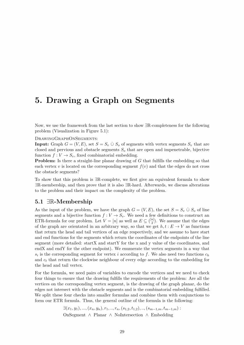
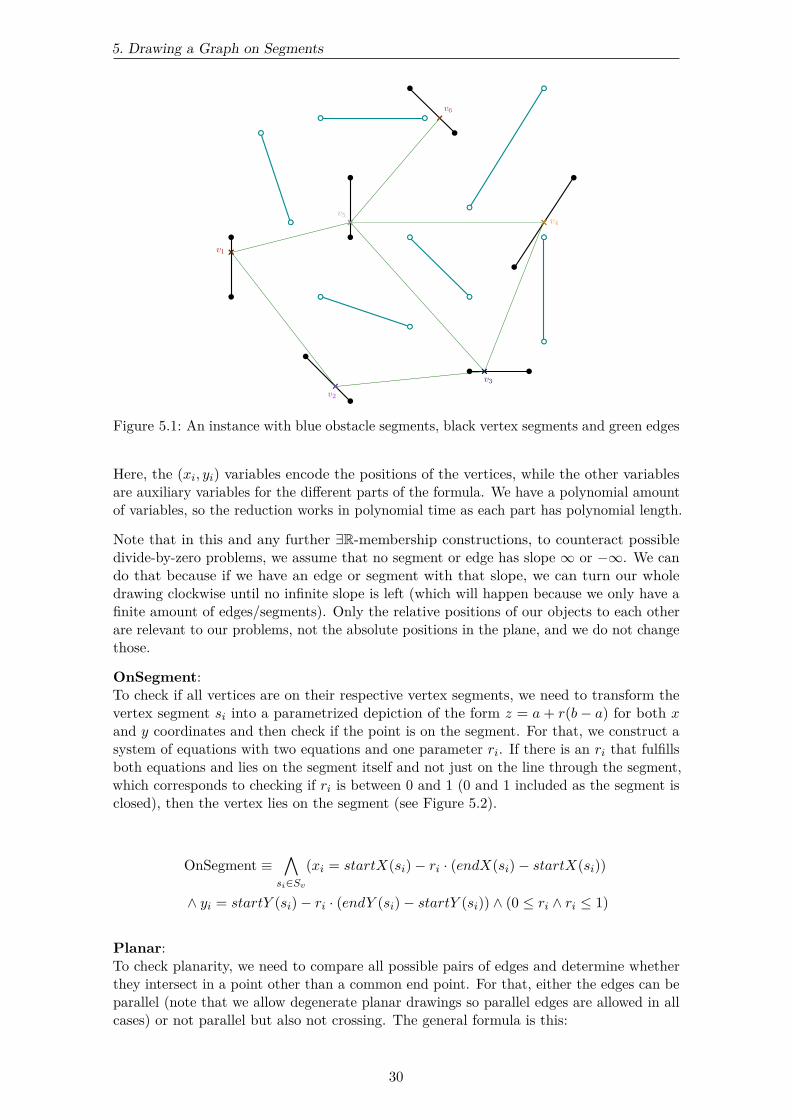
Now, we use the framework from the last section to show ∃R-completeness for the followingproblem (Visualization in Figure 5.1):DrawingGraphOnSegments:Input: Graph G = (V,E), set S = Sv ∪ So of segments with vertex segments Sv that areclosed and pervious and obstacle segments So that are open and impenetrable, bijectivefunction f : V → Sv, fixed combinatorial embedding.Problem: Is there a straight-line planar drawing of G that fulfills the embedding so thateach vertex v is located on the corresponding segment f(v) and that the edges do not crossthe obstacle segments?To show that this problem is ∃R-complete, we first give an equivalent formula to show∃R-membership, and then prove that it is also ∃R-hard. Afterwards, we discuss alterationsto the problem and their impact on the complexity of the problem.
5.1 ∃R-MembershipAs the input of the problem, we have the graph G = (V,E), the set S = Sv ∪ So of linesegments and a bijective function f : V → Sv. We need a few definitions to construct anETR-formula for our problem. Let V = [n] as well as E ⊆
([n]2). We assume that the edges
of the graph are orientated in an arbitrary way, so that we get h, t : E → V as functionsthat return the head and tail vertices of an edge respectively, and we assume to have startand end functions for the segments which return the coordinates of the endpoints of the linesegment (more detailed: startX and startY for the x and y value of the coordinates, andendX and endY for the other endpoint). We enumerate the vertex segments in a way thatsi is the corresponding segment for vertex i according to f . We also need two functions ch
and ct that return the clockwise neighbour of every edge according to the embedding forthe head and tail vertex.For the formula, we need pairs of variables to encode the vertices and we need to checkfour things to ensure that the drawing fulfills the requirements of the problem: Are all thevertices on the corresponding vertex segment, is the drawing of the graph planar, do theedges not intersect with the obstacle segments and is the combinatorial embedding fulfilled.We split these four checks into smaller formulas and combine them with conjunctions toform our ETR formula. Thus, the general outline of the formula is the following:
∃(x1, y1), ..., (xn, yn), r1, .., rn, (s1,2, t1,2), .., (sm−1,m, tm−1,m) :OnSegment ∧ Planar ∧ NoIntersection ∧ Embedding
29
5. Drawing a Graph on Segments
v1
v2
v3
v4
v6
v5
Figure 5.1: An instance with blue obstacle segments, black vertex segments and green edges
Here, the (xi, yi) variables encode the positions of the vertices, while the other variablesare auxiliary variables for the different parts of the formula. We have a polynomial amountof variables, so the reduction works in polynomial time as each part has polynomial length.
Note that in this and any further ∃R-membership constructions, to counteract possibledivide-by-zero problems, we assume that no segment or edge has slope ∞ or −∞. We cando that because if we have an edge or segment with that slope, we can turn our wholedrawing clockwise until no infinite slope is left (which will happen because we only have afinite amount of edges/segments). Only the relative positions of our objects to each otherare relevant to our problems, not the absolute positions in the plane, and we do not changethose.
OnSegment:To check if all vertices are on their respective vertex segments, we need to transform thevertex segment si into a parametrized depiction of the form z = a+ r(b− a) for both xand y coordinates and then check if the point is on the segment. For that, we construct asystem of equations with two equations and one parameter ri. If there is an ri that fulfillsboth equations and lies on the segment itself and not just on the line through the segment,which corresponds to checking if ri is between 0 and 1 (0 and 1 included as the segment isclosed), then the vertex lies on the segment (see Figure 5.2).
OnSegment ≡∧
si∈Sv
(xi = startX(si)− ri · (endX(si)− startX(si))
∧ yi = startY (si)− ri · (endY (si)− startY (si)) ∧ (0 ≤ ri ∧ ri ≤ 1)
Planar:To check planarity, we need to compare all possible pairs of edges and determine whetherthey intersect in a point other than a common end point. For that, either the edges can beparallel (note that we allow degenerate planar drawings so parallel edges are allowed in allcases) or not parallel but also not crossing. The general formula is this:
30
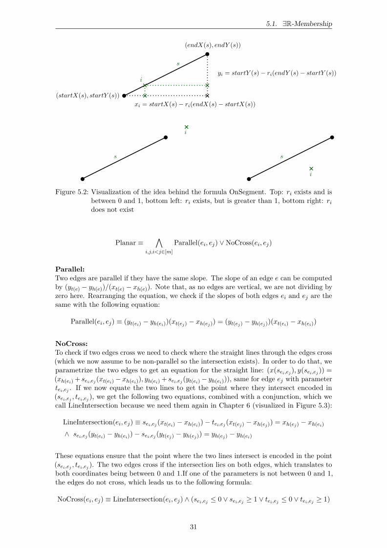
5.1. ∃R-Membership
s
i
(startX(s), startY (s))
(endX(s), endY (s))
xi = startX(s)− ri(endX(s)− startX(s))
yi = startY (s)− ri(endY (s)− startY (s))
s
i
s
i
Figure 5.2: Visualization of the idea behind the formula OnSegment. Top: ri exists and isbetween 0 and 1, bottom left: ri exists, but is greater than 1, bottom right: ri
does not exist
Planar ≡∧
i,j,i<j∈[m]Parallel(ei, ej) ∨NoCross(ei, ej)
Parallel:Two edges are parallel if they have the same slope. The slope of an edge e can be computedby (yt(e) − yh(e))/(xt(e) − xh(e)). Note that, as no edges are vertical, we are not dividing byzero here. Rearranging the equation, we check if the slopes of both edges ei and ej are thesame with the following equation:
Parallel(ei, ej) ≡ (yt(ei) − yh(ei))(xt(ej) − xh(ej)) = (yt(ej) − yh(ej))(xt(ei) − xh(ei))
NoCross:To check if two edges cross we need to check where the straight lines through the edges cross(which we now assume to be non-parallel so the intersection exists). In order to do that, weparametrize the two edges to get an equation for the straight line: (x(sei,ej ), y(sei,ej )) =(xh(ei) + sei,ej (xt(ei)−xh(ei)), yh(ei) + sei,ej (yt(ei)− yh(ei))), same for edge ej with parametertei,ej . If we now equate the two lines to get the point where they intersect encoded in(sei,ej , tei,ej ), we get the following two equations, combined with a conjunction, which wecall LineIntersection because we need them again in Chapter 6 (visualized in Figure 5.3):
LineIntersection(ei, ej) ≡ sei,ej (xt(ei) − xh(ei))− tei,ej (xt(ej) − xh(ej)) = xh(ej) − xh(ei)
∧ sei,ej (yt(ei) − yh(ei))− sei,ej (yt(ej) − yh(ej)) = yh(ej) − yh(ei)
These equations ensure that the point where the two lines intersect is encoded in the point(sei,ej , tei,ej ). The two edges cross if the intersection lies on both edges, which translates toboth coordinates being between 0 and 1.If one of the parameters is not between 0 and 1,the edges do not cross, which leads us to the following formula:
NoCross(ei, ej) ≡ LineIntersection(ei, ej) ∧ (sei,ej ≤ 0 ∨ sei,ej ≥ 1 ∨ tei,ej ≤ 0 ∨ tei,ej ≥ 1)
31
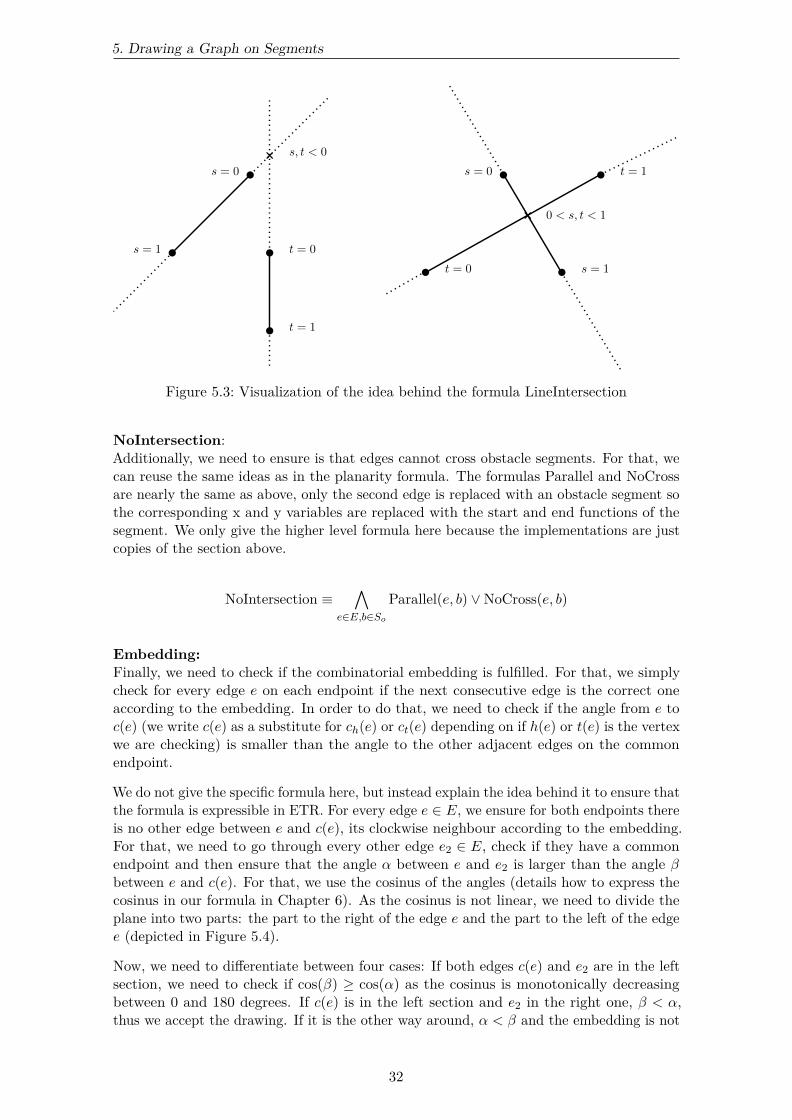
5. Drawing a Graph on Segments
s = 0
s = 1 t = 0
t = 1
s, t < 0
s = 0
s = 1
t = 1
t = 0
0 < s, t < 1
Figure 5.3: Visualization of the idea behind the formula LineIntersection
NoIntersection:Additionally, we need to ensure is that edges cannot cross obstacle segments. For that, wecan reuse the same ideas as in the planarity formula. The formulas Parallel and NoCrossare nearly the same as above, only the second edge is replaced with an obstacle segment sothe corresponding x and y variables are replaced with the start and end functions of thesegment. We only give the higher level formula here because the implementations are justcopies of the section above.
NoIntersection ≡∧
e∈E,b∈So
Parallel(e, b) ∨NoCross(e, b)
Embedding:Finally, we need to check if the combinatorial embedding is fulfilled. For that, we simplycheck for every edge e on each endpoint if the next consecutive edge is the correct oneaccording to the embedding. In order to do that, we need to check if the angle from e toc(e) (we write c(e) as a substitute for ch(e) or ct(e) depending on if h(e) or t(e) is the vertexwe are checking) is smaller than the angle to the other adjacent edges on the commonendpoint.
We do not give the specific formula here, but instead explain the idea behind it to ensure thatthe formula is expressible in ETR. For every edge e ∈ E, we ensure for both endpoints thereis no other edge between e and c(e), its clockwise neighbour according to the embedding.For that, we need to go through every other edge e2 ∈ E, check if they have a commonendpoint and then ensure that the angle α between e and e2 is larger than the angle βbetween e and c(e). For that, we use the cosinus of the angles (details how to express thecosinus in our formula in Chapter 6). As the cosinus is not linear, we need to divide theplane into two parts: the part to the right of the edge e and the part to the left of the edgee (depicted in Figure 5.4).
Now, we need to differentiate between four cases: If both edges c(e) and e2 are in the leftsection, we need to check if cos(β) ≥ cos(α) as the cosinus is monotonically decreasingbetween 0 and 180 degrees. If c(e) is in the left section and e2 in the right one, β < α,thus we accept the drawing. If it is the other way around, α < β and the embedding is not
32
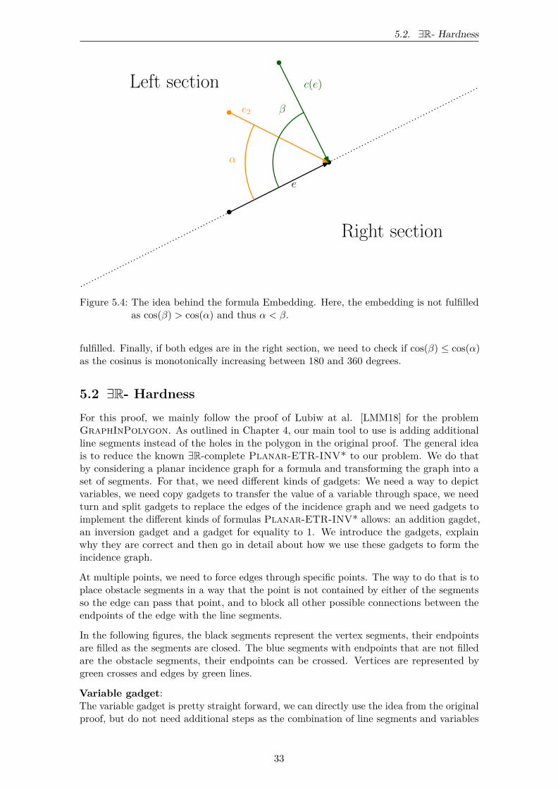
5.2. ∃R- Hardness
Left section
Right section
α
β
e
e2
c(e)
Figure 5.4: The idea behind the formula Embedding. Here, the embedding is not fulfilledas cos(β) > cos(α) and thus α < β.
fulfilled. Finally, if both edges are in the right section, we need to check if cos(β) ≤ cos(α)as the cosinus is monotonically increasing between 180 and 360 degrees.
5.2 ∃R- HardnessFor this proof, we mainly follow the proof of Lubiw at al. [LMM18] for the problemGraphInPolygon. As outlined in Chapter 4, our main tool to use is adding additionalline segments instead of the holes in the polygon in the original proof. The general ideais to reduce the known ∃R-complete Planar-ETR-INV* to our problem. We do thatby considering a planar incidence graph for a formula and transforming the graph into aset of segments. For that, we need different kinds of gadgets: We need a way to depictvariables, we need copy gadgets to transfer the value of a variable through space, we needturn and split gadgets to replace the edges of the incidence graph and we need gadgets toimplement the different kinds of formulas Planar-ETR-INV* allows: an addition gagdet,an inversion gadget and a gadget for equality to 1. We introduce the gadgets, explainwhy they are correct and then go in detail about how we use these gadgets to form theincidence graph.
At multiple points, we need to force edges through specific points. The way to do that is toplace obstacle segments in a way that the point is not contained by either of the segmentsso the edge can pass that point, and to block all other possible connections between theendpoints of the edge with the line segments.
In the following figures, the black segments represent the vertex segments, their endpointsare filled as the segments are closed. The blue segments with endpoints that are not filledare the obstacle segments, their endpoints can be crossed. Vertices are represented bygreen crosses and edges by green lines.
Variable gadget:The variable gadget is pretty straight forward, we can directly use the idea from the originalproof, but do not need additional steps as the combination of line segments and variables
33
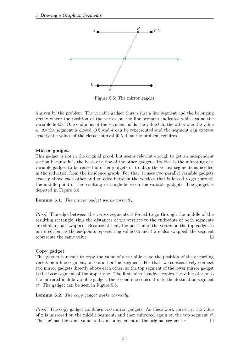
5. Drawing a Graph on Segments
0.5 4x
x′0.54
Figure 5.5: The mirror gagdet
is given by the problem. The variable gadget thus is just a line segment and the belongingvertex where the position of the vertex on the line segment indicates which value thevariable holds. One endpoint of the segment holds the value 0.5, the other one the value4. As the segment is closed, 0.5 and 4 can be represented and the segment can expressexactly the values of the closed interval [0.5, 4] as the problem requires.
Mirror gadget:This gadget is not in the original proof, but seems relevant enough to get an independentsection because it is the basis of a few of the other gadgets. Its idea is the mirroring of avariable gadget to be reused in other gadgets or to align the vertex segments as neededin the reduction from the incidence graph. For that, it uses two parallel variable gadgetsexactly above each other and an edge between the vertices that is forced to go throughthe middle point of the resulting rectangle between the variable gadgets. The gadget isdepicted in Figure 5.5.
Lemma 5.1. The mirror gadget works correctly.
Proof. The edge between the vertex segments is forced to go through the middle of theresulting rectangle, thus the distances of the vertices to the endpoints of both segmentsare similar, but swapped. Because of that, the position of the vertex on the top gadget ismirrored, but as the endpoints representing value 0.5 and 4 are also swapped, the segmentrepresents the same value.
Copy gadget:This gagdet is meant to copy the value of a variable x, so the position of the accordingvertex on a line segment, onto another line segment. For that, we consecutively connecttwo mirror gadgets directly above each other, so the top segment of the lower mirror gadgetis the base segment of the upper one. The first mirror gadget copies the value of x ontothe mirrored middle variable gadget, the second one copies it onto the destination segmentx′. The gadget can be seen in Figure 5.6.
Lemma 5.2. The copy gadget works correctly.
Proof. The copy gadget combines two mirror gadgets. As these work correctly, the valueof x is mirrored on the middle segment, and then mirrored again on the top segment x′.Thus, x′ has the same value and same alignement as the original segment x.
34
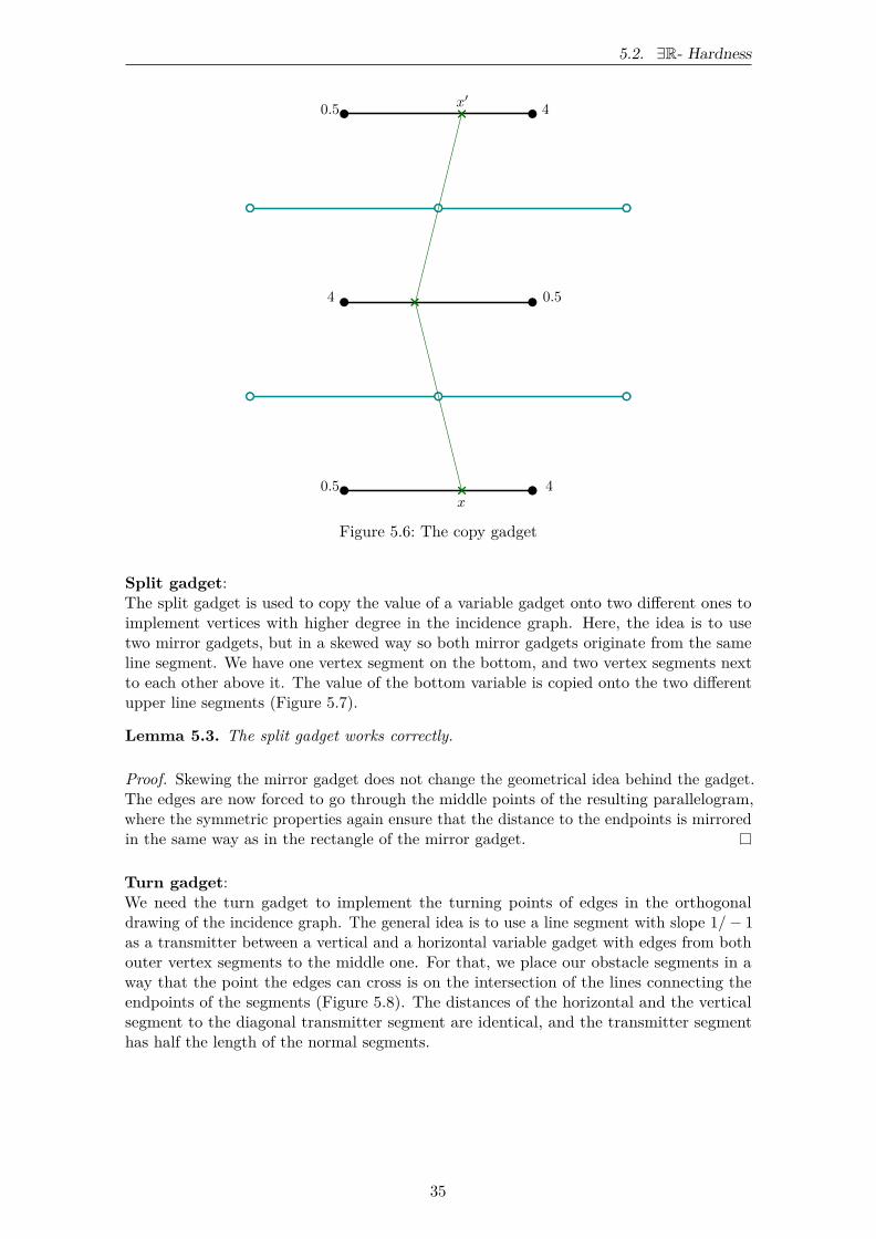
5.2. ∃R- Hardness
0.5 4
4 0.5
40.5
x
x′
Figure 5.6: The copy gadget
Split gadget:The split gadget is used to copy the value of a variable gadget onto two different ones toimplement vertices with higher degree in the incidence graph. Here, the idea is to usetwo mirror gadgets, but in a skewed way so both mirror gadgets originate from the sameline segment. We have one vertex segment on the bottom, and two vertex segments nextto each other above it. The value of the bottom variable is copied onto the two differentupper line segments (Figure 5.7).
Lemma 5.3. The split gadget works correctly.
Proof. Skewing the mirror gadget does not change the geometrical idea behind the gadget.The edges are now forced to go through the middle points of the resulting parallelogram,where the symmetric properties again ensure that the distance to the endpoints is mirroredin the same way as in the rectangle of the mirror gadget.
Turn gadget:We need the turn gadget to implement the turning points of edges in the orthogonaldrawing of the incidence graph. The general idea is to use a line segment with slope 1/− 1as a transmitter between a vertical and a horizontal variable gadget with edges from bothouter vertex segments to the middle one. For that, we place our obstacle segments in away that the point the edges can cross is on the intersection of the lines connecting theendpoints of the segments (Figure 5.8). The distances of the horizontal and the verticalsegment to the diagonal transmitter segment are identical, and the transmitter segmenthas half the length of the normal segments.
35
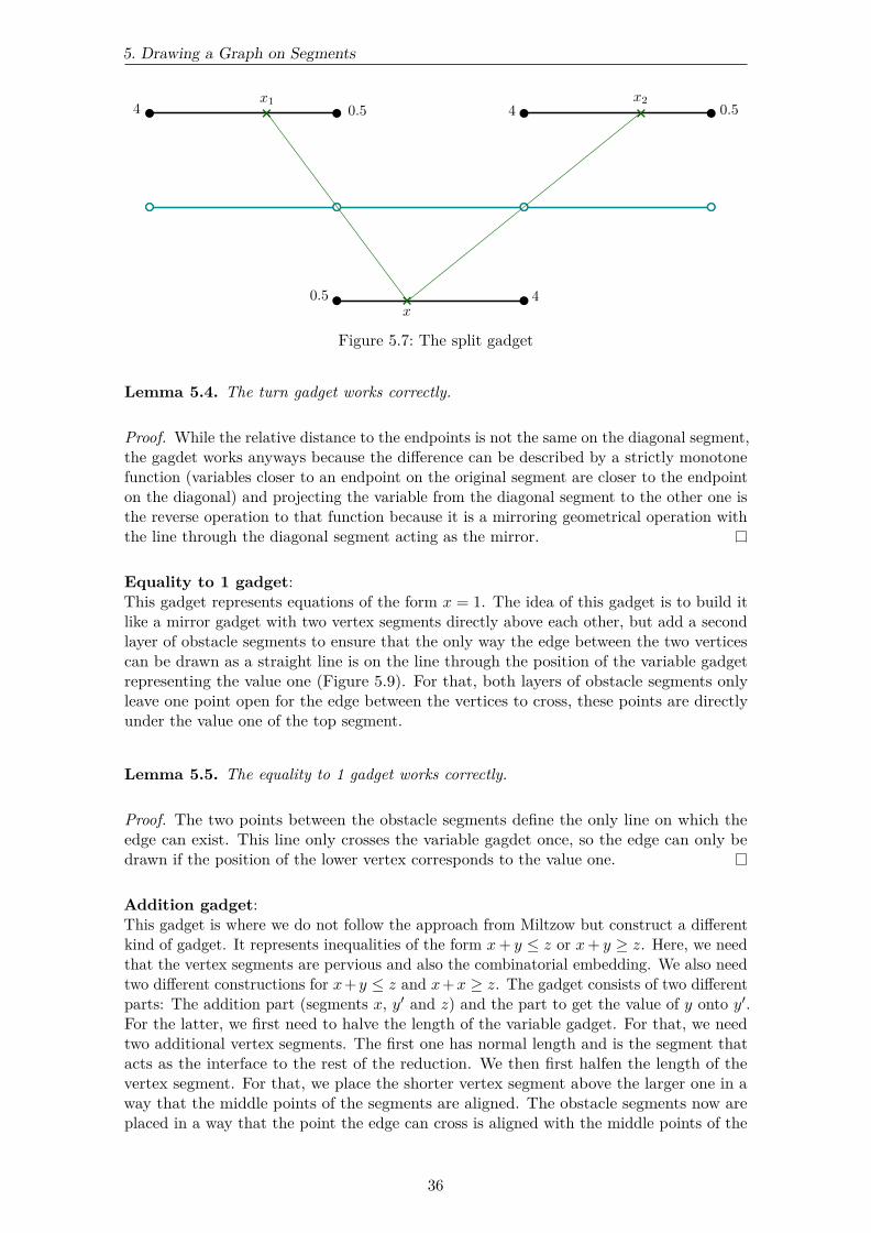
5. Drawing a Graph on Segments
0.5 4
4 0.5 4 0.5
x
x1 x2
Figure 5.7: The split gadget
Lemma 5.4. The turn gadget works correctly.
Proof. While the relative distance to the endpoints is not the same on the diagonal segment,the gagdet works anyways because the difference can be described by a strictly monotonefunction (variables closer to an endpoint on the original segment are closer to the endpointon the diagonal) and projecting the variable from the diagonal segment to the other one isthe reverse operation to that function because it is a mirroring geometrical operation withthe line through the diagonal segment acting as the mirror.
Equality to 1 gadget:This gadget represents equations of the form x = 1. The idea of this gadget is to build itlike a mirror gadget with two vertex segments directly above each other, but add a secondlayer of obstacle segments to ensure that the only way the edge between the two verticescan be drawn as a straight line is on the line through the position of the variable gadgetrepresenting the value one (Figure 5.9). For that, both layers of obstacle segments onlyleave one point open for the edge between the vertices to cross, these points are directlyunder the value one of the top segment.
Lemma 5.5. The equality to 1 gadget works correctly.
Proof. The two points between the obstacle segments define the only line on which theedge can exist. This line only crosses the variable gagdet once, so the edge can only bedrawn if the position of the lower vertex corresponds to the value one.
Addition gadget:This gadget is where we do not follow the approach from Miltzow but construct a differentkind of gadget. It represents inequalities of the form x+ y ≤ z or x+ y ≥ z. Here, we needthat the vertex segments are pervious and also the combinatorial embedding. We also needtwo different constructions for x+y ≤ z and x+x ≥ z. The gadget consists of two differentparts: The addition part (segments x, y′ and z) and the part to get the value of y onto y′.For the latter, we first need to halve the length of the variable gadget. For that, we needtwo additional vertex segments. The first one has normal length and is the segment thatacts as the interface to the rest of the reduction. We then first halfen the length of thevertex segment. For that, we place the shorter vertex segment above the larger one in away that the middle points of the segments are aligned. The obstacle segments now areplaced in a way that the point the edge can cross is aligned with the middle points of the
36
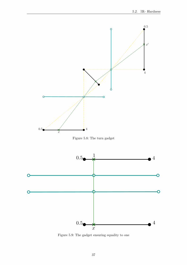
5.2. ∃R- Hardness
0.5 4
4
0.5
x
x′
Figure 5.8: The turn gadget
0.5 4
0.5 41
x
Figure 5.9: The gadget ensuring equality to one
37
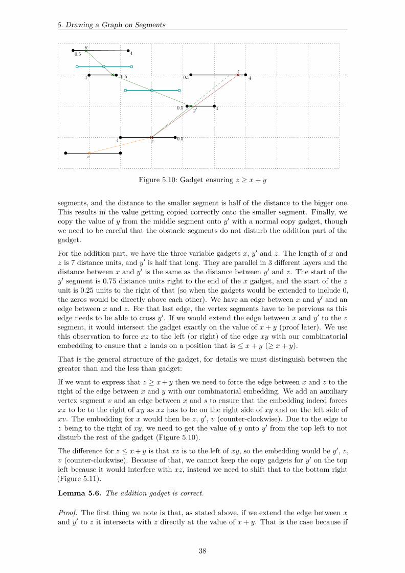
5. Drawing a Graph on Segments
4 0.5
0.5 4
0.5 44 0.5
0.5 4
v
x
y′
z
y
Figure 5.10: Gadget ensuring z ≥ x+ y
segments, and the distance to the smaller segment is half of the distance to the bigger one.This results in the value getting copied correctly onto the smaller segment. Finally, wecopy the value of y from the middle segment onto y′ with a normal copy gadget, thoughwe need to be careful that the obstacle segments do not disturb the addition part of thegadget.
For the addition part, we have the three variable gadgets x, y′ and z. The length of x andz is 7 distance units, and y′ is half that long. They are parallel in 3 different layers and thedistance between x and y′ is the same as the distance between y′ and z. The start of they′ segment is 0.75 distance units right to the end of the x gadget, and the start of the zunit is 0.25 units to the right of that (so when the gadgets would be extended to include 0,the zeros would be directly above each other). We have an edge between x and y′ and anedge between x and z. For that last edge, the vertex segments have to be pervious as thisedge needs to be able to cross y′. If we would extend the edge between x and y′ to the zsegment, it would intersect the gadget exactly on the value of x+ y (proof later). We usethis observation to force xz to the left (or right) of the edge xy with our combinatorialembedding to ensure that z lands on a position that is ≤ x+ y (≥ x+ y).
That is the general structure of the gadget, for details we must distinguish between thegreater than and the less than gadget:
If we want to express that z ≥ x+ y then we need to force the edge between x and z to theright of the edge between x and y with our combinatorial embedding. We add an auxiliaryvertex segment v and an edge between x and s to ensure that the embedding indeed forcesxz to be to the right of xy as xz has to be on the right side of xy and on the left side ofxv. The embedding for x would then be z, y′, v (counter-clockwise). Due to the edge toz being to the right of xy, we need to get the value of y onto y′ from the top left to notdisturb the rest of the gadget (Figure 5.10).
The difference for z ≤ x+ y is that xz is to the left of xy, so the embedding would be y′, z,v (counter-clockwise). Because of that, we cannot keep the copy gadgets for y′ on the topleft because it would interfere with xz, instead we need to shift that to the bottom right(Figure 5.11).
Lemma 5.6. The addition gadget is correct.
Proof. The first thing we note is that, as stated above, if we extend the edge between xand y′ to z it intersects with z directly at the value of x+ y. That is the case because if
38
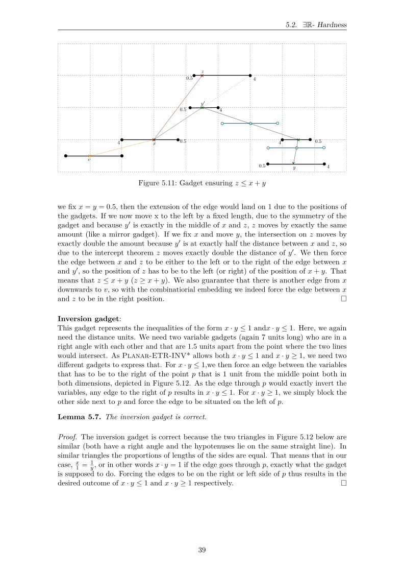
5.2. ∃R- Hardness
4 0.5
0.5 4
0.5 4
4 0.5
0.5 4
v
x
y′
z
y
Figure 5.11: Gadget ensuring z ≤ x+ y
we fix x = y = 0.5, then the extension of the edge would land on 1 due to the positions ofthe gadgets. If we now move x to the left by a fixed length, due to the symmetry of thegadget and because y′ is exactly in the middle of x and z, z moves by exactly the sameamount (like a mirror gadget). If we fix x and move y, the intersection on z moves byexactly double the amount because y′ is at exactly half the distance between x and z, sodue to the intercept theorem z moves exactly double the distance of y′. We then forcethe edge between x and z to be either to the left or to the right of the edge between xand y′, so the position of z has to be to the left (or right) of the position of x+ y. Thatmeans that z ≤ x+ y (z ≥ x+ y). We also guarantee that there is another edge from xdownwards to v, so with the combinatiorial embedding we indeed force the edge between xand z to be in the right position.
Inversion gadget:This gadget represents the inequalities of the form x · y ≤ 1 andx · y ≤ 1. Here, we againneed the distance units. We need two variable gadgets (again 7 units long) who are in aright angle with each other and that are 1.5 units apart from the point where the two lineswould intersect. As Planar-ETR-INV* allows both x · y ≤ 1 and x · y ≥ 1, we need twodifferent gadgets to express that. For x · y ≤ 1,we then force an edge between the variablesthat has to be to the right of the point p that is 1 unit from the middle point both inboth dimensions, depicted in Figure 5.12. As the edge through p would exactly invert thevariables, any edge to the right of p results in x · y ≤ 1. For x · y ≥ 1, we simply block theother side next to p and force the edge to be situated on the left of p.
Lemma 5.7. The inversion gadget is correct.
Proof. The inversion gadget is correct because the two triangles in Figure 5.12 below aresimilar (both have a right angle and the hypotenuses lie on the same straight line). Insimilar triangles the proportions of lengths of the sides are equal. That means that in ourcase, x
1 = 1y , or in other words x · y = 1 if the edge goes through p, exactly what the gadget
is supposed to do. Forcing the edges to be on the right or left side of p thus results in thedesired outcome of x · y ≤ 1 and x · y ≥ 1 respectively.
39
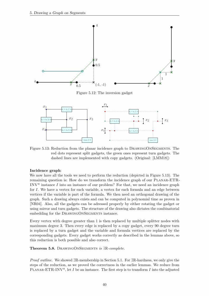
5. Drawing a Graph on Segments
40.5
0.5
4
(-1, -1)x
y
x
y
1
1
Figure 5.12: The inversion gadget
x1 + x2 ≤ x3
x1
x3x2
x4
x1 + x2 ≥ x4
x2 + x4 ≤ x3
x3x4 ≤ 1
x1 + x2 ≤ x3
x1
x3x2
x4
x1 + x2 ≥ x4
x2 + x4 ≤ x3
x3x4 ≤ 1
Figure 5.13: Reduction from the planar incidence graph to DrawingOnSegments. Thered dots represent split gadgets, the green ones represent turn gadgets. Thedashed lines are implemented with copy gadgets. (Original: [LMM18])
Incidence graph:We now have all the tools we need to perform the reduction (depicted in Figure 5.13). Theremaining question is: How do we transform the incidence graph of our Planar-ETR-INV* instance I into an instance of our problem? For that, we need an incidence graphfor I. We have a vertex for each variable, a vertex for each formula and an edge betweenvertices if the variable is part of the formula. We then need an orthogonal drawing of thegraph. Such a drawing always exists and can be computed in polynomial time as proven in[NR04]. Also, all the gadgets can be adressed properly by either rotating the gadget orusing mirror and turn gadgets. The structure of the drawing also dictates the combinatorialembedding for the DrawingOnSegments instance.
Every vertex with degree greater than 1 is then replaced by multiple splitter nodes withmaximum degree 3. Then every edge is replaced by a copy gadget, every 90 degree turnis replaced by a turn gadget and the variable and formula vertices are replaced by thecorresponding gadgets. Every gadget works correctly as described in the lemmas above, sothis reduction is both possible and also correct.
Theorem 5.8. DrawingOnSegments is ∃R-complete.
Proof outline. We showed ∃R-membership in Section 5.1. For ∃R-hardness, we only give thesteps of the reduction, as we proved the correctness in the earlier lemmas. We reduce fromPlanar-ETR-INV*, let I be an instance. The first step is to transform I into the adjusted
40
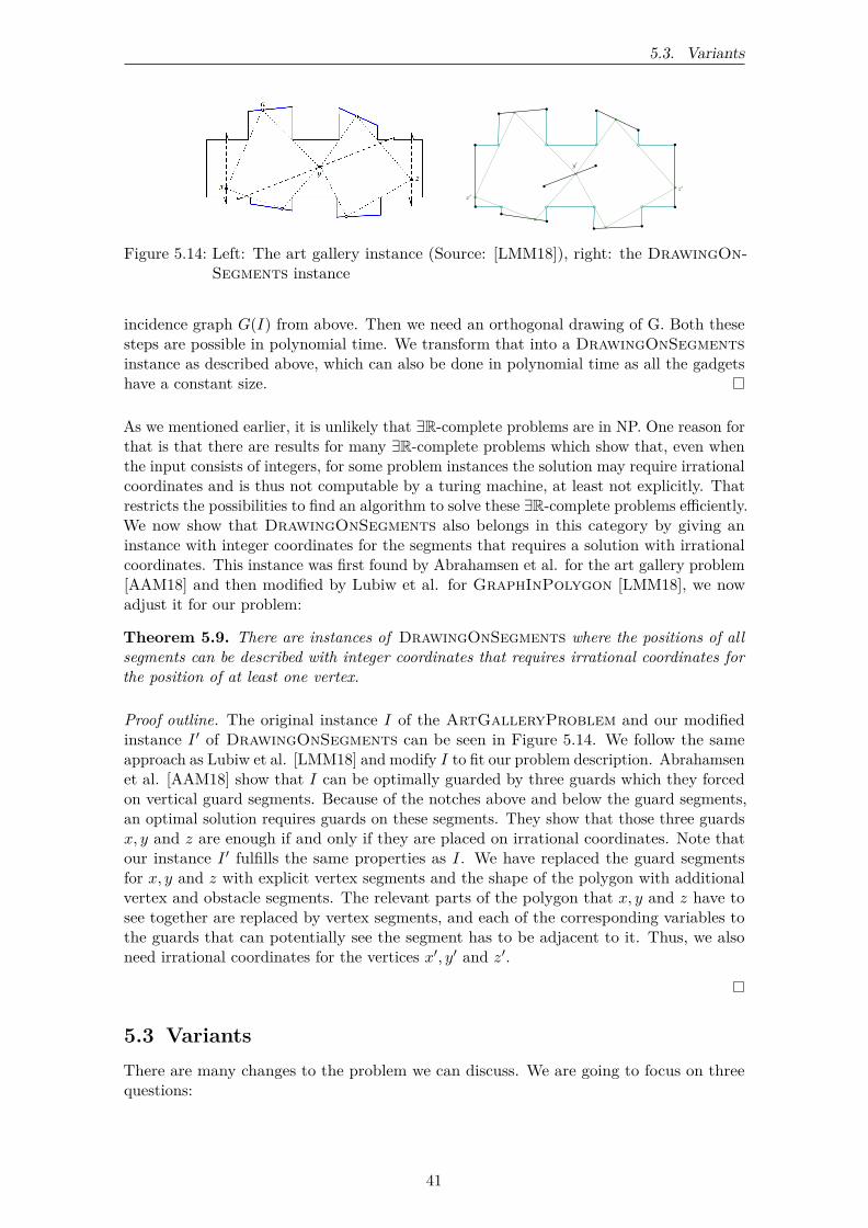
5.3. Variants
x′
y′
z′
Figure 5.14: Left: The art gallery instance (Source: [LMM18]), right: the DrawingOn-Segments instance
incidence graph G(I) from above. Then we need an orthogonal drawing of G. Both thesesteps are possible in polynomial time. We transform that into a DrawingOnSegmentsinstance as described above, which can also be done in polynomial time as all the gadgetshave a constant size.
As we mentioned earlier, it is unlikely that ∃R-complete problems are in NP. One reason forthat is that there are results for many ∃R-complete problems which show that, even whenthe input consists of integers, for some problem instances the solution may require irrationalcoordinates and is thus not computable by a turing machine, at least not explicitly. Thatrestricts the possibilities to find an algorithm to solve these ∃R-complete problems efficiently.We now show that DrawingOnSegments also belongs in this category by giving aninstance with integer coordinates for the segments that requires a solution with irrationalcoordinates. This instance was first found by Abrahamsen et al. for the art gallery problem[AAM18] and then modified by Lubiw et al. for GraphInPolygon [LMM18], we nowadjust it for our problem:
Theorem 5.9. There are instances of DrawingOnSegments where the positions of allsegments can be described with integer coordinates that requires irrational coordinates forthe position of at least one vertex.
Proof outline. The original instance I of the ArtGalleryProblem and our modifiedinstance I ′ of DrawingOnSegments can be seen in Figure 5.14. We follow the sameapproach as Lubiw et al. [LMM18] and modify I to fit our problem description. Abrahamsenet al. [AAM18] show that I can be optimally guarded by three guards which they forcedon vertical guard segments. Because of the notches above and below the guard segments,an optimal solution requires guards on these segments. They show that those three guardsx, y and z are enough if and only if they are placed on irrational coordinates. Note thatour instance I ′ fulfills the same properties as I. We have replaced the guard segmentsfor x, y and z with explicit vertex segments and the shape of the polygon with additionalvertex and obstacle segments. The relevant parts of the polygon that x, y and z have tosee together are replaced by vertex segments, and each of the corresponding variables tothe guards that can potentially see the segment has to be adjacent to it. Thus, we alsoneed irrational coordinates for the vertices x′, y′ and z′.
5.3 VariantsThere are many changes to the problem we can discuss. We are going to focus on threequestions:
41
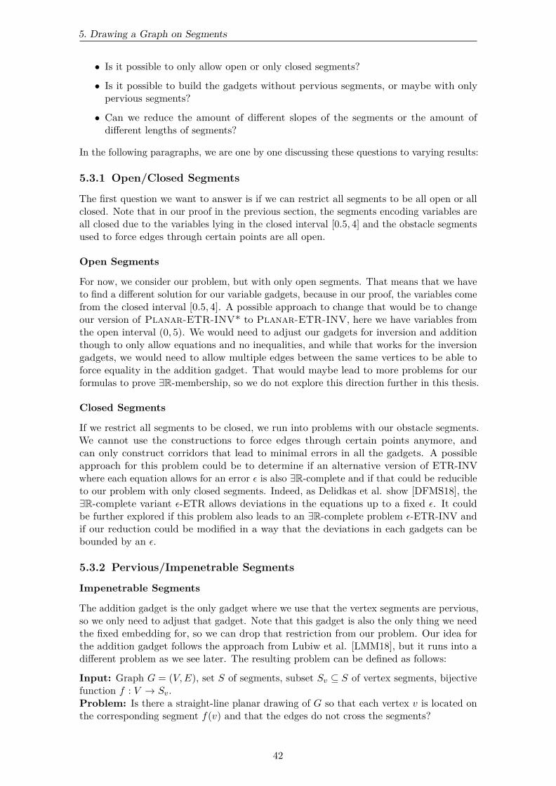
5. Drawing a Graph on Segments
• Is it possible to only allow open or only closed segments?
• Is it possible to build the gadgets without pervious segments, or maybe with onlypervious segments?
• Can we reduce the amount of different slopes of the segments or the amount ofdifferent lengths of segments?
In the following paragraphs, we are one by one discussing these questions to varying results:
5.3.1 Open/Closed Segments
The first question we want to answer is if we can restrict all segments to be all open or allclosed. Note that in our proof in the previous section, the segments encoding variables areall closed due to the variables lying in the closed interval [0.5, 4] and the obstacle segmentsused to force edges through certain points are all open.
Open Segments
For now, we consider our problem, but with only open segments. That means that we haveto find a different solution for our variable gadgets, because in our proof, the variables comefrom the closed interval [0.5, 4]. A possible approach to change that would be to changeour version of Planar-ETR-INV* to Planar-ETR-INV, here we have variables fromthe open interval (0, 5). We would need to adjust our gadgets for inversion and additionthough to only allow equations and no inequalities, and while that works for the inversiongadgets, we would need to allow multiple edges between the same vertices to be able toforce equality in the addition gadget. That would maybe lead to more problems for ourformulas to prove ∃R-membership, so we do not explore this direction further in this thesis.
Closed Segments
If we restrict all segments to be closed, we run into problems with our obstacle segments.We cannot use the constructions to force edges through certain points anymore, andcan only construct corridors that lead to minimal errors in all the gadgets. A possibleapproach for this problem could be to determine if an alternative version of ETR-INVwhere each equation allows for an error ε is also ∃R-complete and if that could be reducibleto our problem with only closed segments. Indeed, as Delidkas et al. show [DFMS18], the∃R-complete variant ε-ETR allows deviations in the equations up to a fixed ε. It couldbe further explored if this problem also leads to an ∃R-complete problem ε-ETR-INV andif our reduction could be modified in a way that the deviations in each gadgets can bebounded by an ε.
5.3.2 Pervious/Impenetrable Segments
Impenetrable Segments
The addition gadget is the only gadget where we use that the vertex segments are pervious,so we only need to adjust that gadget. Note that this gadget is also the only thing we needthe fixed embedding for, so we can drop that restriction from our problem. Our idea forthe addition gadget follows the approach from Lubiw et al. [LMM18], but it runs into adifferent problem as we see later. The resulting problem can be defined as follows:
Input: Graph G = (V,E), set S of segments, subset Sv ⊆ S of vertex segments, bijectivefunction f : V → Sv.Problem: Is there a straight-line planar drawing of G so that each vertex v is located onthe corresponding segment f(v) and that the edges do not cross the segments?
42
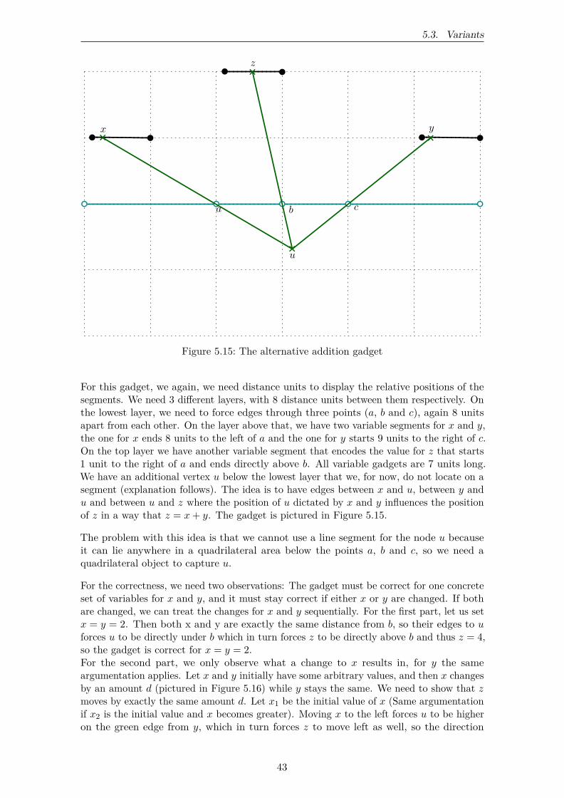
5.3. Variants
u
x y
z
a b c
Figure 5.15: The alternative addition gadget
For this gadget, we again, we need distance units to display the relative positions of thesegments. We need 3 different layers, with 8 distance units between them respectively. Onthe lowest layer, we need to force edges through three points (a, b and c), again 8 unitsapart from each other. On the layer above that, we have two variable segments for x and y,the one for x ends 8 units to the left of a and the one for y starts 9 units to the right of c.On the top layer we have another variable segment that encodes the value for z that starts1 unit to the right of a and ends directly above b. All variable gadgets are 7 units long.We have an additional vertex u below the lowest layer that we, for now, do not locate on asegment (explanation follows). The idea is to have edges between x and u, between y andu and between u and z where the position of u dictated by x and y influences the positionof z in a way that z = x+ y. The gadget is pictured in Figure 5.15.
The problem with this idea is that we cannot use a line segment for the node u becauseit can lie anywhere in a quadrilateral area below the points a, b and c, so we need aquadrilateral object to capture u.
For the correctness, we need two observations: The gadget must be correct for one concreteset of variables for x and y, and it must stay correct if either x or y are changed. If bothare changed, we can treat the changes for x and y sequentially. For the first part, let us setx = y = 2. Then both x and y are exactly the same distance from b, so their edges to uforces u to be directly under b which in turn forces z to be directly above b and thus z = 4,so the gadget is correct for x = y = 2.For the second part, we only observe what a change to x results in, for y the sameargumentation applies. Let x and y initially have some arbitrary values, and then x changesby an amount d (pictured in Figure 5.16) while y stays the same. We need to show that zmoves by exactly the same amount d. Let x1 be the initial value of x (Same argumentationif x2 is the initial value and x becomes greater). Moving x to the left forces u to be higheron the green edge from y, which in turn forces z to move left as well, so the direction
43
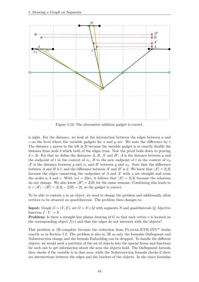
5. Drawing a Graph on Segments
dt
2t
x1x2
A
A′BB′
Figure 5.16: The alternative addition gadget is correct.
is right. For the distance, we look at the intersection between the edges between u andz on the level where the variable gadgets for x and y are. We note the difference by t.The distance z moves to the left is 2t because the variable gadget is at exactly double thedistance from node b which both of the edges cross. Now the proof boils down to provingd = 2t. For that we define the distances A, B, A′ and B′: A is the distance between y andthe endpoint of t in the context of x1, B to the new endpoint of t in the context of x2.A′ is the distance between y and x1 and B′ between y and x2. Note that the differencebetween A and B is t, and the difference between A′ and B′ is d. We know that |A′| = 2|A|because the edges connecting the endpoints of A and A′ with u are straight and crossthe nodes a, b and c. With |ac| = 2|bc|, it follows that |A′| = 2|A| because the relationsdo not change. We also know |B′| = 2|B| for the same reasons. Combining this leads tod = |A′| − |B′| = 2|A| − 2|B| = 2t, so the gadget is correct.
To be able to contain u in an object, we need to change the problem and additionally allowvertices to be situated on quadrilaterals. The problem then changes to:
Input: Graph G = (V,E), set O = S ∪Q with segments S and quadrilaterals Q, bijectivefunction f : V → S.Problem: Is there a straight-line planar drawing of G so that each vertex v is located onthe corresponding object f(v) and that the edges do not intersect with the objects?
This problem is ∃R-complete because the reduction from Planar-ETR-INV* worksexactly as in Section 5.2. The problem is also in ∃R as only the formulas OnSegment andNoIntersection change and the formula Embedding can be dropped. To handle the differentobjects, we would need a partition of the set of objects into the special forms and functionsfor each one to get information about the area the objects hold. The OnSegment formulathen checks if the variable is in that area, while the NoIntersection formula checks if thereare intersections between the edges and the borders of the objects. In the exact formulas
44
5.3. Variants
for quadrilaterals, the NoIntersection formula would need to check for intersections betweenedges and all 4 sides of the rectangle.
Pervious Segments
If on the other hand we drop the requirement that the edges should not intersect with thesegments, all of the gadgets are suddenly not possible anymore because we have no toolsto force certain edges through fixed points. We do not see a way to recreate the gadgets.That is why this iteration of the problem is somewhat likely to not be ∃R-complete.
5.3.3 Using only few Slopes/Lengths
We currently have 4 different slopes in our constructions: horizontal and vertical segmentsand segments with slope 1/-1 for the turn gadget. Because of the way the reduction fromthe incidence graph is done, we for sure need the horizontal and vertical segments. It isalso not possible to drop the segments of slope 1/-1 in the turn segment, because whentrying to directly convert the value of a horizontal to a vertical segment and vice versa,the ratio of the distance to the endpoints is always changed by a function f. We need toundo that function by mirroring the operation, and to end up on a segment turned by 90degrees, we need a segment of slope 1/-1 in the middle.When trying to unify the length of each segment, we run into similar problems with theaddition gadget. Either y’ or z needs to have a different length than the other, becausechanging the position of the node on y’ causes double that change on z. However, we canrestrict the lengths of all segments to either 3.5 or 7 distance units, with the shorter onesonly used for the addition gadget and the turn gadget.
45

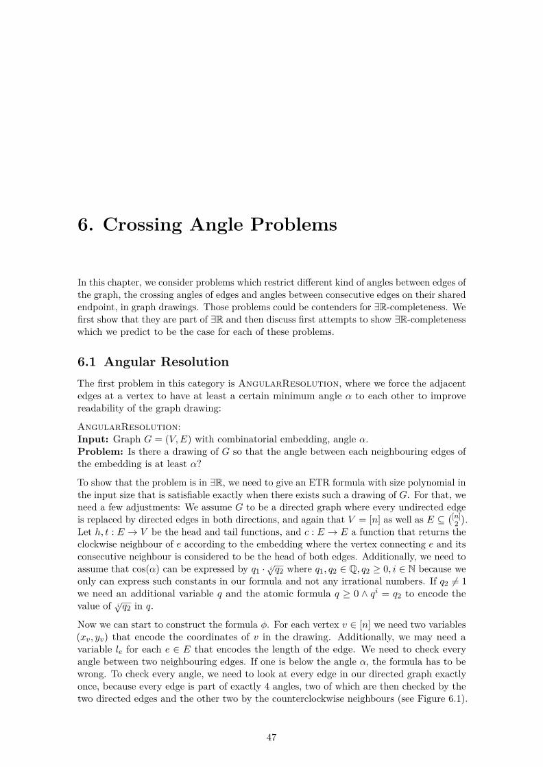
6. Crossing Angle Problems
In this chapter, we consider problems which restrict different kind of angles between edges ofthe graph, the crossing angles of edges and angles between consecutive edges on their sharedendpoint, in graph drawings. Those problems could be contenders for ∃R-completeness. Wefirst show that they are part of ∃R and then discuss first attempts to show ∃R-completenesswhich we predict to be the case for each of these problems.
6.1 Angular ResolutionThe first problem in this category is AngularResolution, where we force the adjacentedges at a vertex to have at least a certain minimum angle α to each other to improvereadability of the graph drawing:
AngularResolution:Input: Graph G = (V,E) with combinatorial embedding, angle α.Problem: Is there a drawing of G so that the angle between each neighbouring edges ofthe embedding is at least α?
To show that the problem is in ∃R, we need to give an ETR formula with size polynomial inthe input size that is satisfiable exactly when there exists such a drawing of G. For that, weneed a few adjustments: We assume G to be a directed graph where every undirected edgeis replaced by directed edges in both directions, and again that V = [n] as well as E ⊆
([n]2).
Let h, t : E → V be the head and tail functions, and c : E → E a function that returns theclockwise neighbour of e according to the embedding where the vertex connecting e and itsconsecutive neighbour is considered to be the head of both edges. Additionally, we need toassume that cos(α) can be expressed by q1 · i
√q2 where q1, q2 ∈ Q, q2 ≥ 0, i ∈ N because we
only can express such constants in our formula and not any irrational numbers. If q2 6= 1we need an additional variable q and the atomic formula q ≥ 0 ∧ qi = q2 to encode thevalue of i
√q2 in q.
Now we can start to construct the formula φ. For each vertex v ∈ [n] we need two variables(xv, yv) that encode the coordinates of v in the drawing. Additionally, we may need avariable le for each e ∈ E that encodes the length of the edge. We need to check everyangle between two neighbouring edges. If one is below the angle α, the formula has to bewrong. To check every angle, we need to look at every edge in our directed graph exactlyonce, because every edge is part of exactly 4 angles, two of which are then checked by thetwo directed edges and the other two by the counterclockwise neighbours (see Figure 6.1).
47
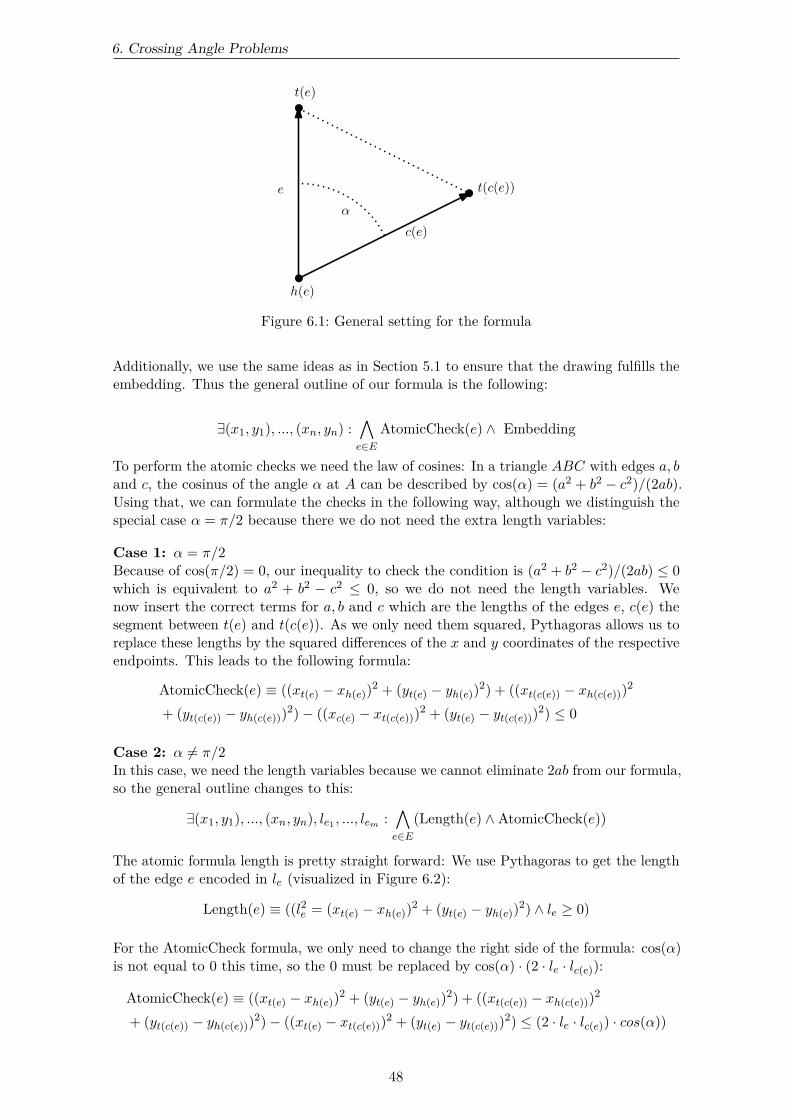
6. Crossing Angle Problems
e
c(e)
h(e)
t(e)
t(c(e))
α
Figure 6.1: General setting for the formula
Additionally, we use the same ideas as in Section 5.1 to ensure that the drawing fulfills theembedding. Thus the general outline of our formula is the following:
∃(x1, y1), ..., (xn, yn) :∧
e∈E
AtomicCheck(e) ∧ Embedding
To perform the atomic checks we need the law of cosines: In a triangle ABC with edges a, band c, the cosinus of the angle α at A can be described by cos(α) = (a2 + b2 − c2)/(2ab).Using that, we can formulate the checks in the following way, although we distinguish thespecial case α = π/2 because there we do not need the extra length variables:
Case 1: α = π/2Because of cos(π/2) = 0, our inequality to check the condition is (a2 + b2 − c2)/(2ab) ≤ 0which is equivalent to a2 + b2 − c2 ≤ 0, so we do not need the length variables. Wenow insert the correct terms for a, b and c which are the lengths of the edges e, c(e) thesegment between t(e) and t(c(e)). As we only need them squared, Pythagoras allows us toreplace these lengths by the squared differences of the x and y coordinates of the respectiveendpoints. This leads to the following formula:
AtomicCheck(e) ≡ ((xt(e) − xh(e))2 + (yt(e) − yh(e))2) + ((xt(c(e)) − xh(c(e)))2
+ (yt(c(e)) − yh(c(e)))2)− ((xc(e) − xt(c(e)))2 + (yt(e) − yt(c(e)))2) ≤ 0
Case 2: α 6= π/2In this case, we need the length variables because we cannot eliminate 2ab from our formula,so the general outline changes to this:
∃(x1, y1), ..., (xn, yn), le1 , ..., lem :∧
e∈E
(Length(e) ∧AtomicCheck(e))
The atomic formula length is pretty straight forward: We use Pythagoras to get the lengthof the edge e encoded in le (visualized in Figure 6.2):
Length(e) ≡ ((l2e = (xt(e) − xh(e))2 + (yt(e) − yh(e))2) ∧ le ≥ 0)
For the AtomicCheck formula, we only need to change the right side of the formula: cos(α)is not equal to 0 this time, so the 0 must be replaced by cos(α) · (2 · le · lc(e)):
AtomicCheck(e) ≡ ((xt(e) − xh(e))2 + (yt(e) − yh(e))2) + ((xt(c(e)) − xh(c(e)))2
+ (yt(c(e)) − yh(c(e)))2)− ((xt(e) − xt(c(e)))2 + (yt(e) − yt(c(e)))2) ≤ (2 · le · lc(e)) · cos(α))
48
6.2. Right Angle Crosing Drawings
e
h(e)
t(e)
yt(e) − yh(e)
xt(e) − xh(e)
Figure 6.2: Visualization of the idea behind the formula Length
This formula is sufficient because if cos(β) for the angle β between e and c(e) is greaterthan cos(α), then either β < α or the remaining angle 2π − β < α and either way there isan angle that violates the condition of the problem.
We note that, while this version of the problem admits a shorter formula, we can also showthat we do not need to fix a combinatorial embedding to find a formula that solves theproblem. We use mainly the same ideas as in the formula above, but replace the function cby simply checking pairs of edges, and check the angle between them if they are adjacent,that is if the head of the edges is the same. The outline of the formula is following, Lengthstays the same and in AtomicCheck each c(e) is assumed to be replaced by e2:
∃(x1, y1), ..., (xn, yn), le1 , ..., lem : (∧
e∈E
Length(e))
∧ (∧
e1,e2,e1 6=e2∈E
h(e1) 6= h(e2) ∨ AtomicCheck(e1, e2))
6.2 Right Angle Crosing Drawings
Another way to make graph drawings easier to read for humans is to ensure that twoedges only cross in a right angle to prevent edges that run almost parallel and cross. Theemerging problem is the following:
RAC-DrawingInput: Graph G = (V,E).Problem: Is there a drawing of G with straight-line edges where on each internal crossingbetween two edges the crossing angles are right angles?
To prove ∃R-membership for this problem we again need a few modifications: We againassume that G is a directed graph with V = [n], although this time, it is sufficient to simplyorientate each edge in an arbitrary way to gain a defined head and tail for our functions hand t which we will need again.
This time, the problem requires us to look at pairs of edges and check if they cross and ifthey do so in a right angle. For that, we again need the variables (xi, yi) for the coordinatesof the vertices, but we also need pairs (sei,ej , tei,ej )(i, j ∈ [m], i < j) to check for crossingsbetween edges. Then we need to iterate over each pair of edges and check if one of three
49
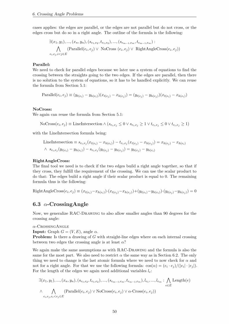
6. Crossing Angle Problems
cases applies: the edges are parallel, or the edges are not parallel but do not cross, or theedges cross but do so in a right angle. The outline of the formula is the following:
∃(x1, y1), ..., (xn, yn), (se1,e2 , te1,e2), ..., (sem−1,em , tem−1,em) :∧ei,ej ,i<j∈E
(Parallel(ei, ej) ∨ NoCross (ei, ej) ∨ RightAngleCross(ei, ej))
Parallel:We need to check for parallel edges because we later use a system of equations to find thecrossing between the straights going to the two edges. If the edges are parallel, then thereis no solution to the system of equations, so it has to be handled explicitly. We can reusethe formula from Section 5.1:
Parallel(ei, ej) ≡ (yt(ei) − yh(ei))(xt(ej) − xh(ej)) = (yt(ej) − yh(ej))(xt(ei) − xh(ei))
NoCross:We again can reuse the formula from Section 5.1:
NoCross(ei, ej) ≡ LineIntersection ∧ (sei,ej ≤ 0 ∨ sei,ej ≥ 1 ∨ tei,ej ≤ 0 ∨ tei,ej ≥ 1)
with the LineIntersection formula being:
LineIntersection ≡ sei,ej (xt(ei) − xh(ei))− tei,ej (xt(ej) − xh(ej)) = xh(ej) − xh(ei)
∧ sei,ej (yt(ei) − yh(ei))− sei,ej (yt(ej) − yh(ej)) = yh(ej) − yh(ei)
RightAngleCross:The final tool we need is to check if the two edges build a right angle together, so that ifthey cross, they fulfill the requirement of the crossing. We can use the scalar product todo that: The edges build a right angle if their scalar product is equal to 0. The remainingformula thus is the following:
RightAngleCross(ei, ej) ≡ (xt(ei)−xh(ei))·(xt(ej)−xh(ej))+(yt(ei)−yh(ei))·(yt(ej)−yh(ej)) = 0
6.3 α-CrossingAngleNow, we generalize RAC-Drawing to also allow smaller angles than 90 degrees for thecrossing angle:
α-CrossingAngleInput: Graph G = (V,E), angle α.Problem: Is there a drawing of G with straight-line edges where on each internal crossingbetween two edges the crossing angle is at least α?
We again make the same assumptions as with RAC-Drawing and the formula is also thesame for the most part. We also need to restrict α the same way as in Section 6.2. The onlything we need to change is the last atomic formula where we need to now check for α andnot for a right angle. For that we use the following formula: cos(α) = (ei · ej)/(|ei| · |ej |).For the length of the edges we again need additional variables le:
∃(x1, y1), ..., (xn, yn), (se1,e2 , te1,e2), ..., (sem−1,em , tem−1,em), le1 , ..., lem :∧
e∈E
Length(e)
∧∧
ei,ej ,ei<ej∈E
(Parallel(ei, ej) ∨NoCross(ei, ej) ∨ α-Cross(ei, ej))
50
6.4. ∃R-Completeness
We reuse the formulas Length, Parallel and NoCross, only α-Cross needs to be defined.For that, we need to check if (a · b)/(|a| · |b|) is both smaller than cos(α) and greater than− cos(α) because we do not know if we look at the smaller or the greater angle at thecrossing and if and only if both inequalities are fulfilled, all the crossing angles are at leastα. Thus, the following formula, again restructured to avoid fractions, is sufficient:
α-Cross(ei, ej) ≡ ((xt(ei) − xh(ei)) · (xt(ej) − xh(ej))+ (yt(ei) − yh(ei)) · (yt(ej) − yh(ej)) ≤ cos(α) · lei · lej )∨ ((xt(eI) − xh(ei)) · (xt(ej) − xh(ej)) + (yt(ei) − yh(ei)) · (yt(ej) − yh(ej)) ≥ −cos(α) · lei · lej )
6.4 ∃R-CompletenessWe tried to follow the same approach as in Chapter 5 to prove ∃R-completeness for each ofthese problems, but ran into problems along the way for all of them. It is somewhat likelythat they are indeed ∃R-complete as it was proven that certain special cases of the problemsare NP-hard with no obvious way to show that they are also part of NP. RAC-Drawingwas proven to be NP-hard by Argyriou et al. [ABS11] and AngularResolution, atleast for graphs with maximum degree four, was also proven NP-hard by Formann et al.[FHH+93]. The reductions only work for variables with boolean values though, and cannotbe modified to represent real values as well.
We suspect that these problems are in fact ∃R-complete, without having a concrete approachfor proving that. Maybe it is possible to build all the gadgets for the ETR-INV-proof,maybe it is easier to find a reduction from SimpleStretchability, but the generalproperties of the problems (geometrical graph drawing problems, known for being NP-hard,but not yet proven to be part of NP) are very similar to known ∃R-complete problems.
51

7. Conclusion
In this thesis, we considered the Existential Theory of the Reals and explored the cor-responding complexity class ∃R, especially the problems that are complete in ∃R. Weshowed that ∃R lies inbetween NP and PSPACE and found an equivalent machine modell.After that, we presented different variants of ETR, notably Feasibility, ETR-INV andthe planar variants of ETR-INV in Chapter 3 as possible starting points for ∃R-hardnessreductions. We then treated the problem SimpleStretchability as another base forreductions and summarized many of those reductions that were done in the last years,notably the reductions to RECOG(SEG) and GraphInPolygon in detail. Also inChapter 4, we presented the blueprint introduced by Miltzow et al. for reductions fromETR-INV and its planar variants and explained three reductions that follow this framework,to prove that the Art Gallery Problem, GraphInPolygon and PrescribedAreaPE are∃R-complete.
Our main goal was to characterize the existing reductions, find a way to replicate themeasily and apply that to conduct our own ∃R-completeness proof. As described above,we did the first part in Chapter 4. In Chapter 5, we then successfully implementedthat framework for a reduction from Planar-ETR-INV* to show ∃R-completeness of ournew problem DrawingOnSegments. For that, we constructed an ETR formula forDrawingOnSegments, created the necessary gadgets for the reduction from Planar-ETR-INV* and explained the transformation from an incidence graph to the graph drawinginstance. Finally, we showed ∃R-membership for the graph drawing problems dealing withangular issues, AngularResolution, RAC-Drawing and α-CrossingAngle.
Open questions
A few questions remained open in these last two sections. While we found a few interestingfacts about variants of the DrawingOnSegments problem, notably another slightlydifferent ∃R-complete version of the problem, there is more to explore in this setting: Ifwe have only impenetrable segments, is there a way to design the addition gadget thatdoes not require a quadrilateral object? If we have only closed segments, can we find anETR-INV variant that allows us to conduct a modified ∃R-hardness proof? And if we onlyhave pervious segments, does the problem remain ∃R-complete or does it maybe shift intoNP?
53
7. Conclusion
The main open questions from our thesis are the ones from Chapter 6: Are the problemsAngular Resolution, RAC-Drawing and α-CrossingAngle indeed ∃R-complete?They are NP-hard, at least for special cases, with no obvious way to prove NP-membership,and we showed that they belong in ∃R. Because of that, we believe that it is likely thatthey could be shown to be ∃R-complete in the future and gave some first approaches howsuch a proof could be conducted. While our attempts to create all the gadgets necessaryfor an ETR-INV based ∃R-hardness proof have failed, maybe there are ways to do itsuccessfully. It could also be easier to base the reductions on SimpleStretchability, orother ∃R-complete problems that are more similar to these angular problems.
54
Bibliography
[AAM18] Mikkel Abrahamsen, Anna Adamaszek, and Tillmann Miltzow. The art galleryproblem is ∃R-complete. In Proceedings of the 50th Annual ACM SIGACTSymposium on Theory of Computing, pages 65–73, 2018.
[ABB+20] Oswin Aichholzer, Manuel Borrazzo, Prosenjit Bose, Jean Cardinal, FabrizioFrati, Pat Morin, and Birgit Vogtenhuber. Drawing graphs as spanners. arXivpreprint arXiv:2002.05580, 2020.
[ABS11] Evmorfia N Argyriou, Michael A Bekos, and Antonios Symvonis. The straight-line RAC drawing problem is NP-hard. In International Conference on CurrentTrends in Theory and Practice of Computer Science, pages 74–85. Springer,2011.
[AM19] Mikkel Abrahamsen and Tillmann Miltzow. Dynamic Toolbox for ETRINV.arXiv preprint arXiv:1912.08674, 2019.
[AMS20] Mikkel Abrahamsen, Tillmann Miltzow, and Nadja Seiferth. Frameworkfor ∃R-Completeness of Two-Dimensional Packing Problems. arXiv preprintarXiv:2004.07558, 2020.
[BC06] Peter Bürgisser and Felipe Cucker. Counting complexity classes for numericcomputations II: Algebraic and semialgebraic sets. Journal of Complexity,22(2):147–191, 2006.
[Bie91] Daniel Bienstock. Some provably hard crossing number problems. Discrete &Computational Geometry, 6(3):443–459, 1991.
[BM16] Vittorio Bilò and Marios Mavronicolas. A catalog of EXISTS-R-completedecision problems about Nash equilibria in multi-player games. In 33rd Sym-posium on Theoretical Aspects of Computer Science (STACS 2016). SchlossDagstuhl-Leibniz-Zentrum fuer Informatik, 2016.
[Bro03] Christopher W Brown. QEPCAD B: a program for computing with semi-algebraic sets using CADs. ACM SIGSAM Bulletin, 37(4):97–108, 2003.
[BSS+89] Lenore Blum, Mike Shub, Steve Smale, et al. On a theory of computationand complexity over the real numbers: NP -completeness, recursive functionsand universal machines. Bulletin (New Series) of the American MathematicalSociety, 21(1):1–46, 1989.
[Can88] John Canny. Some algebraic and geometric computations in PSPACE. InProceedings of the twentieth annual ACM symposium on Theory of computing,pages 460–467, 1988.
[Car15] Jean Cardinal. Computational geometry column 62. ACM SIGACT News,46(4):69–78, 2015.
55
Bibliography
[CH17] Jean Cardinal and Udo Hoffmann. Recognition and complexity of point visibilitygraphs. Discrete & Computational Geometry, 57(1):164–178, 2017.
[CK13] Jean Cardinal and Vincent Kusters. The complexity of simultaneous geometricgraph embedding. arXiv preprint arXiv:1302.7127, 2013.
[Col75] George E Collins. Quantifier elimination for real closed fields by cylindricalalgebraic decompostion. In Automata Theory and Formal Languages 2nd GIConference Kaiserslautern, May 20–23, 1975, pages 134–183. Springer, 1975.
[Coo71] Stephen A Cook. The complexity of theorem-proving procedures. In Proceedingsof the third annual ACM symposium on Theory of computing, pages 151–158,1971.
[DFMS18] Argyrios Deligkas, John Fearnley, Themistoklis Melissourgos, and Paul GSpirakis. Approximating the existential theory of the reals. In InternationalConference on Web and Internet Economics, pages 126–139. Springer, 2018.
[DGC99] Ernest Davis, Nicholas Mark Gotts, and Anthony G Cohn. Constraint networksof topological relations and convexity. Constraints, 4(3):241–280, 1999.
[DKMR18] Michael Gene Dobbins, Linda Kleist, Tillmann Miltzow, and Paweł Rzążewski.∀∃R-Completeness and Area-Universality. In International Workshop on Graph-Theoretic Concepts in Computer Science, pages 164–175. Springer, 2018.
[Eri19] Jeff Erickson. Optimal Curve Straightening is ∃R-Complete. arXiv preprintarXiv:1908.09400, 2019.
[FHH+93] Michael Formann, Torben Hagerup, James Haralambides, Michael Kaufmann,Frank Thomson Leighton, Antonios Symvonis, Emo Welzl, and G Woeginger.Drawing graphs in the plane with high resolution. SIAM Journal on Computing,22(5):1035–1052, 1993.
[Gra07] Erich Graedel. Finite model theory and descriptive complexity. In Finite modeltheory and its applications, pages 125–230. Springer, 2007.
[GVJ88] D Yu Grigor’ev and Nikolaj N Vorobjov Jr. Solving systems of polynomialinequalities in subexponential time. Journal of symbolic computation, 5(1-2):37–64, 1988.
[H+91] Hoon Hong et al. Comparison of several decision algorithms for the existentialtheory of the reals. Citeseer, 1991.
[Hof17] Udo Hoffmann. On the Complexity of the Planar Slope Number Problem. J.Graph Algorithms Appl., 21(2):183–193, 2017.
[HRS93] Joos Heintz, M-F Roy, and Pablo Solernó. On the theoretical and practicalcomplexity of the existential theory of reals. The Computer Journal, 36(5):427–431, 1993.
[Kyn11] Jan Kynčl. Simple realizability of complete abstract topological graphs in p.Discrete & Computational Geometry, 45(3):383–399, 2011.
[LMM18] Anna Lubiw, Tillmann Miltzow, and Debajyoti Mondal. The complexity ofdrawing a graph in a polygonal region. In International Symposium on GraphDrawing and Network Visualization, pages 387–401. Springer, 2018.
[Mat14] Jiri Matousek. Intersection graphs of segments and ∃R. arXiv preprintarXiv:1406.2636, 2014.
56
Bibliography
[MM13] Colin McDiarmid and Tobias Müller. Integer realizations of disk and segmentgraphs. Journal of Combinatorial Theory, Series B, 103(1):114–143, 2013.
[Mnë88] Nikolai E Mnëv. The universality theorems on the classification problemof configuration varieties and convex polytopes varieties. In Topology andgeometry—Rohlin seminar, pages 527–543. Springer, 1988.
[NR04] Takao Nishizeki and Md Saidur Rahman. Planar graph drawing, volume 12.World Scientific Publishing Company, 2004.
[Ren88] James Renegar. A faster PSPACE algorithm for deciding the existential theoryof the reals. Technical report, Cornell University Operations Research andIndustrial Engineering, 1988.
[Sch09] Marcus Schaefer. Complexity of some geometric and topological problems. InInternational Symposium on Graph Drawing, pages 334–344. Springer, 2009.
[Sch13] Marcus Schaefer. Realizability of graphs and linkages. In Thirty Essays onGeometric Graph Theory, pages 461–482. Springer, 2013.
[Sch14] Marcus Schaefer. Picking planar edges; or, drawing a graph with a planar sub-graph. In International Symposium on Graph Drawing, pages 13–24. Springer,2014.
[Sho] Peter W Shor. Stretchability of pseudolines is NP-hard, Applied geometry anddiscrete mathematics, 1991. MR1116375 (92g: 05065), pages 531–554.
[SŠ17] Marcus Schaefer and Daniel Štefankovič. Fixed points, Nash equilibria, and theexistential theory of the reals. Theory of Computing Systems, 60(2):172–193,2017.
[Tar98] Alfred Tarski. A decision method for elementary algebra and geometry. InQuantifier elimination and cylindrical algebraic decomposition, pages 24–84.Springer, 1998.
57