Computing the graph-based parallel complexity

of gene assembly

Artiom Alhazov2 ∗, Chang Li2, Ion Petre1,2

1Academy of Finland

2Department of IT, Abo Akademi University

Turku Center for Computer Science, FIN-20520 Turku, Finland

{aalhazov,lchang,ipetre}@abo.fi

Abstract

We consider a graph-theoretical formalization of the process of geneassembly in ciliates introduced in Ehrenfeucht et al (2003), where a geneis modeled as a signed graph. The gene assembly, based on three typesof operations only, is then modeled as a graph reduction process (to theempty graph). Motivated by the robustness of the gene assembly process,the notions of parallel reduction and parallel complexity of signed graphshave been considered in Harju et al (2006). We describe in this paper anexact algorithm for computing the parallel complexity of a given signedgraph and for finding an optimal parallel reduction for it. Checking theparallel applicability of a given set of operations and scanning all pos-sible selections amount to a high computational complexity. However,an example shows that a faster approximate algorithm cannot guaranteefinding the optimal reduction.

Keywords: Gene assembly; Parallelism; Signed graphs; Parallel complex-ity; Algorithmics.

1 Introduction

Ciliates are an old and diverse group of unicellular eukaryotes. One of theirunique features is that they have two types of functionally different nuclei, eachpresent in multiple copies in each cell: micronuclei and macronuclei. Micronucleiare the germline nuclei, where no transcription takes place, while the macronu-clei are the somatic nuclei. The difference between the micronuclear and the

∗A.Alhazov is on leave of absence from Institute of Mathematics and Computer Sci-ence, Academy of Sciences of Moldova Str. Academiei 5, Chisinau, MD-2028, Moldova,aartiom@math.md

1

macronuclear genome is striking, especially in Stichotrichs, on which we concen-trate in the following. Thus, while macronuclear genes are contiguous sequencesplaced in general on their own molecules, micronuclear genes are placed on longchromosomes, interrupted by stretches of non-coding material. Even more strik-ing is that the micronuclear genes are split into several blocks (up to 44 blocksin certain species), with the blocks arranged in a shuffled order, separated bynon-coding material. Some blocks may even be inverted! At some stage duringsexual reproduction, ciliates assemble the blocks in the orthodox order to yieldthe transcription able macronuclear gene. In this process, ciliates make use ofsome short specific sequences at the extremities of each MDS in the same wayas pointers are used in computer science. Indeed, each coding block ends witha short sequence of nucleotides that is repeated in the beginning of the codingblock that should follow it in the orthodox order. We refer to [13], [9] for moredetails on ciliates and on gene assembly.

Two mathematical models were introduced for gene assembly: an inter-molecular model, see [10], [11] and an intramolecular model, see [3], [14]. Theintramolecular model, that we consider in this paper, has been formalized onseveral levels of abstraction, including permutations, strings, and graphs, see[8] for details and [2] for a monograph on the mathematical theory of gene as-sembly. In the following we will only consider a formalization of genes throughgraphs.

A micronuclear gene may be represented through the (shuffled) sequencesof its coding blocks. Each coding block in turn, may be represented by its pairof left and right pointers. Thus, the block Bi that should come on the i-thposition in the orthodox order, will be denoted as Bi = i(i+ 1). The first blockbegins with a specific marker that we may ignore in our abstraction and denoteB1 = 2. Similarly, the last block will be denoted as Bn = n. If a block Bi comesinverted in the micronuclear gene, then it will be denoted as Bi = (i + 1)i. Assuch, a micronuclear gene may be denoted as a signed double occurrence string,see [1] for more details. On a different level of abstraction, one may replace thesigned double occurrence string with its correspondent signed overlap graph.For a micronuclear gene consisting of n coding blocks, n ≥ 1, and having theassociated string u, its corresponding signed overlap graph will have the formGu = ({2, . . . , n}, Eu, σu), where

• ij ∈ Eu if and only if i and j overlap in u, i.e., u = u1i′u2j

′u3i”u4j”u5 oru = u1j

′u2i′u3j”u4i”u5, for some strings ui, 1 ≤ i ≤ 5, where i′, i” ∈ {i, i}

and j′, j” ∈ {j, j}

• σ(i) = + if both i and i occur in u, and σ(i) = − otherwise.

The intramolecular model for gene assembly introduced in [3, 14] consists ofthree molecular operations, whose description we omit here. It is enough for thepurpose of this paper to mention that each operation combines two or, in onecase, even three, coding blocks into a bigger coding block by splicing on theircommon pointers. Since a pointer is only important for gene assembly whenit is placed at the extremity of a coding block (and not when inside a bigger

2

coding block), it follows that the process of gene assembly may be thought ofas a process of removing pointers. Note also that the final assembled gene isa contiguous sequences of nucleotides containing no more pointers. Based onthese observations, the molecular operations of [3, 14] may be formalized asrewriting rules for signed double occurrence strings as well as rewriting rulesfor signed overlap graphs. It may be proved mathematically that as far as geneassembly is concerned, both formalizations are equivalent, with an assembledgene corresponding to the empty string and to the empty graph, see [2] fordetails.

Given the crucial role that parallelism plays in biochemical processes, it isimportant to consider a notion of parallelism in the graph-based mathemati-cal framework for gene assembly. Indeed, parallelism in this context has beendefined in [6] as follows: a set S of operations can be applied in parallel to agraph G if all sequential compositions of operations in S are applicable to G.It is proved in [6] that in this case, all sequential compositions of operations inS lead to the same result when applied to G. This leads to considering parallelreduction strategies for a given graph G, where one applies a number of oper-ations in parallel to G, obtaining a new graph G′ and continues doing so untilobtaining the empty graph. Furthermore, this yields a measure of complexityfor a signed graph in terms of the minimal number of parallel steps needed toreduce the graph to the empty one. This measure of complexity may be relatedto the degree of complexity of the process of gene assembly. It has been shownin [4] that all known ciliate genes may be assembled in at most two parallelsteps. Graphs of higher complexity are known, as summarized in Table 1.

c 1 2 3 4 5 6n 1 2 3 5 12 24

Table 1: The order n of the smallest graphs of complexity c

A number of partial results have been obtained on whether an upper boundexists on the parallel complexity of signed graphs, see [6], [5], [4], but the problemin its full generality remains open.

Open problem: Is the parallel complexity of signed graphs finitely bounded?

Even (seemingly) simpler variants of the problem, where the question is askedfor signed trees or for unsigned graphs, remain open up to date. It has onlybeen shown that the parallel complexity of negative trees is at most two, whilethat of positive trees is at most three, see [7]. On the other hand, examples ofsigned trees of parallel complexity five and examples of signed graphs of parallelcomplexity six are known, see [4]. The difficulty of the problem is perhaps bestillustrated by the fact that no efficient decision procedure is known for whetheror not a given set of operations is applicable to a given graph. As a matter of fact,the only known decision procedure is based on the very definition of parallelismand it involves checking the applicability of all sequential compositions of theoperations, a tedious procedure even for small sets of operations. Computing

3

the parallel complexity of a given gene/graph is even more involved: not onlythat sets of operations must be applied in parallel one after another, but alsoan optimization problem in terms of minimizing the number of parallel stepsneeded to reduce the graph, must be solved.

We describe in this paper an algorithm to compute the parallel complexityof a given signed graph and to find in the same time an optimal parallel re-duction for it. Given the current gaps in the theory of parallel complexity, thealgorithm is essentially based on an exhaustive search. Consequently, it is notsurprising that despite several cut-offs in the search algorithm, its complexityremains huge. We give it here an upper bound on the scale of O

(

n2n+4/dn)

,

for d = e2/√

8, where e is the natural base and n is the number of nodes.It is an open problem whether a faster algorithm can be given based on thecurrent theory of parallelism. We show that, e.g., a Greedy-type of algorithmcannot guarantee finding the optimal parallel reduction (and its complexity re-mains highly exponential). Finally, we present briefly an implementation of thealgorithm.

2 Preliminaries

A signed graph is a triple G = (V, E, σ), where G = (V, E) is an undirected graphand σ : V → {+,−}. Edges between u, v ∈ V are denoted by uv (uv = vu). Welet V + = σ−1(+) and V − = σ−1(−). By NG(u) = {v ∈ V | uv ∈ E} we denotethe neighborhood of u ∈ V .

For signed graphs G1 = (V1, E1, σ1) and G2 = (V2, E2, σ2), we will need thefollowing graph-theoretic operations:

• If V1 ∩ V2 = ∅, then we denote G1 ∪ G2 = (V, E, σ), V = V1 ∪ V2, E =E1 ∪ E2, σ = σ1 ∪ σ2|V2\V1

;

• G1 \G2 = (V1, E1 \ E2, σ1) ;

• G1∆G2 = (G1 \G2) ∪ (G2 \G1).

For a set S ⊆ V we denote by G|S = (S, E ∩ (S × S), σ|S) the subgraphinduced by S. We also write G − S = G|V \S . For a set S ⊆ V we denote byKG(S) = (S, {uv | u, v ∈ S, u 6= v}, σ|S) the clique induced by S. For setsS1, S2 ⊆ V with S1 ∩ S2 = ∅, we use the notation KG(S1, S2) = (S, {uv | u ∈S1, v ∈ S2}, σ|S1∪S2) to represent the complete bipartite graph induced by S1

and S2.For a graph G = (V, E, σ), we denote neg(G) = (V, E, σ′), where σ′(u) = −

if and only if σ(u) = +, u ∈ V the graph obtained from G by complementingits signing. Then com(G) = neg(KG(V ) \G) denotes the graph obtained fromG by complementing both its edges and its signing. For a set S ⊆ V , we denotecomS(G) = com(G|S) ∪ (G \KG(S)). Finally, for a node u ∈ V we denote bylocu(G) = comNG(u)(G) the graph with complemented edges and signing overthe neighborhood of u.

4

3 A graph-based model for gene assembly

We recall in this section the graph-based mathematical framework for geneassembly, as introduced in [1], see also [2].

Definition 1 Consider a signed graph G = (V, E, σ).

• For x ∈ V −, if NG(x) = ∅, then the graph negative rule gnr is applicable

to x and gnrx(G) = G− {x}.

• For x ∈ V +, the graph positive rule gpr is applicable to x and gprx(G) =locx(G)− {x}.

• For xy ∈ V − × V −, the graph double rule gdr is applicable to x, y and

gdrx,y(G) = (G \ {x, y}, E′, σ|V \{x,y}), where E′ is obtained from E by

complementing the edges that join nodes in NG(x) to nodes in NG(y).Thus, for p, q ∈ V \ {x, y}, the edge relationship between p and q will

change if and only if

p ∈ NG(x) \NG(y), and q ∈ NG(y)

p ∈ NG(y) \NG(x), and q ∈ NG(x)

p ∈ NG(x) ∩NG(y), and q ∈ NG(x)∆NG(y)

Example 1 Applications of a gpr operation and a gdr operation are illustrated

in Figure 1.

The sets of all gnr, gpr and gdr operations are denoted by GNR, GPR andGDR, respectively. We also use notations dom(gnrx) = {x}, dom(gprx) ={x} and dom(gdrx,y) = {x, y}. We extend the notation to sets: dom(S) =∪r∈Sdom(r).

For an operation r and a sequential composition ϕ of operations, we saythat ϕ ◦ r is applicable to G if r is applicable to G and ϕ is applicable to r(G)(clearly, ∅ is always applicable to G).

Consider ϕ = rk◦. . .◦r1 where r1, . . . , rk ∈ GNR∪GPR∪GDR. Whenever ϕ isapplicable to G, we define the predicate applicableϕ(G) as true, and we naturallydenote the result by ϕ(G) = rk(. . . (r1(G)) . . .).

4 Parallelism

We recall in this section the notion of parallelism for the reduction of signedgraphs, as introduced in [6].

Definition 2 We say that operations S ⊆ GNR ∪ GPR ∪ GDR are applicable in

parallel to G if any sequential composition of the operations in S is applicable

to G.

5

a)

GFED@ABC1− GFED@ABC2+

mmmmmmmmmmmm

zzzz

zz

GFED@ABC6−DD

DDDD

GFED@ABC7−FF

FFFF

ONMLHIJK11+

llllllllllll

GFED@ABC3− GFED@ABC4+ GFED@ABC5− GFED@ABC8− GFED@ABC9+ ONMLHIJK10−

b)

GFED@ABC1− GFED@ABC6−DD

DDDD

GFED@ABC7−FF

FFFF

ONMLHIJK11+

llllllllllll

GFED@ABC3+ GFED@ABC4− GFED@ABC5+ GFED@ABC8− GFED@ABC9+ ONMLHIJK10−

c)

GFED@ABC1− GFED@ABC2+

mmmmmmmmmmmm

zzzz

zz

ONMLHIJK11+

xxxx

xx

GFED@ABC3− GFED@ABC4+ GFED@ABC5− GFED@ABC8− GFED@ABC9+ ONMLHIJK10−

Figure 1: Graphs a) G, b) gpr2(G) and c) gdr6,7(G).

We recall the following lemma (Theorem 6.4 from [6]).

Lemma 1 ([6]) If S is applicable in parallel to G, then for any two sequential

compositions ϕ1, ϕ2 of the operations in S, we have ϕ1(G) = ϕ2(G).

Therefore, whenever S is applicable in parallel to G, we may consider the graphS(G) obtained by applying S to G as the result of applying the operations of Sto G in an arbitrary order.

We now recall the definition of parallel complexity of signed graphs.

Definition 3 ([5]) Let G be a signed graph. For sets S1, . . . , Sk ⊆ GNR ∪GPR ∪ GDR, we say that R = Sk ◦ . . . ◦ S1 is applicable to G if Si is applicable

to (Si−1 ◦ . . . ◦ S1)(G), for all 1 ≤ i ≤ k. If R(G) = ∅, then we say that R is

a parallel reduction strategy for G. We say that the parallel complexity of R is

C(Sk ◦ . . . ◦ S1) = k. The parallel complexity C(G) of G is defined as

C(G) = min{C(R) | R is a parallel reduction strategy for G}.A parallel reduction strategy R for a graph G is called optimal if C(R) = C(G).

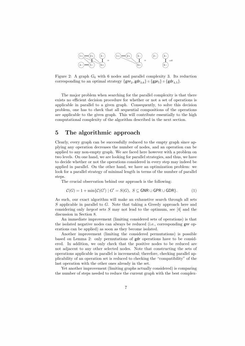
Example 2 An example of a graph, its parallel complexity and an optimal strat-

egy to reduce it in parallel to the empty graph are given in Figure 2.

Consider a signed graph G = (V, E, σ) and sets Vn ⊆ V −∩{u ∈ V | NG(u) =∅}, Vp ⊆ V + and Ed ⊆ E ∩ (V −×V −). Consider the following problem: decidewhether a set S = {gnrx | x ∈ Vn} ∪ {gprx | x ∈ Vp} ∪ {gdrx,y | xy ∈ Vd} ofoperations is applicable to G in parallel. The following lemma summarizes thecurrent partial solution to the problem.

Lemma 2 ([6]) Consider a a signed graph G and a set S ⊂ GNR∪GPR∪GDR

of operations applicable to G. Then S is applicable in parallel to G if and only

if NG|dom(S)(u) = ∅ for all gpru ∈ S and S ∩ GDR is applicable in parallel to G.

6

GFED@ABC1+

DDDD

DD

QQQQQQQQQQQQGFED@ABC2+

DDDD

DDGFED@ABC3−

⇒

GFED@ABC1+

QQQQQQQQQQQQGFED@ABC2+

DDDD

DDGFED@ABC3−

⇒

GFED@ABC2− GFED@ABC3−⇒∅

GFED@ABC4− GFED@ABC5− GFED@ABC6+ GFED@ABC6+ GFED@ABC6−

Figure 2: A graph G6 with 6 nodes and parallel complexity 3. Its reductioncorresponding to an optimal strategy {gnr2, gdr3,6} ◦ {gpr1} ◦ {gdr4,5}.

The major problem when searching for the parallel complexity is that thereexists no efficient decision procedure for whether or not a set of operations isapplicable in parallel to a given graph. Consequently, to solve this decisionproblem, one has to check that all sequential compositions of the operationsare applicable to the given graph. This will contribute essentially to the highcomputational complexity of the algorithm described in the next section.

5 The algorithmic approach

Clearly, every graph can be successfully reduced to the empty graph since ap-plying any operation decreases the number of nodes, and an operation can beapplied to any non-empty graph. We are faced here however with a problem ontwo levels. On one hand, we are looking for parallel strategies, and thus, we haveto decide whether or not the operations considered in every step may indeed beapplied in parallel. On the other hand, we have an optimization problem: welook for a parallel strategy of minimal length in terms of the number of parallelsteps.

The crucial observation behind our approach is the following:

C(G) = 1 + min{C(G′) | G′ = S(G), S ⊆ GNR ∪ GPR ∪ GDR}. (1)

As such, our exact algorithm will make an exhaustive search through all setsS applicable in parallel to G. Note that taking a Greedy approach here andconsidering only largest sets S may not lead to the optimum, see [4] and thediscussion in Section 8.

An immediate improvement (limiting considered sets of operations) is thatthe isolated negative nodes can always be reduced (i.e., corresponding gnr op-erations can be applied) as soon as they become isolated.

Another improvement (limiting the considered permutations) is possiblebased on Lemma 2: only permutations of gdr operations have to be consid-ered. In addition, we only check that the positive nodes to be reduced arenot adjacent to any other selected nodes. Note that constructing the sets ofoperations applicable in parallel is incremental; therefore, checking parallel ap-plicability of an operation set is reduced to checking the “compatibility” of thelast operation with the other ones already in the set.

Yet another improvement (limiting graphs actually considered) is comparingthe number of steps needed to reduce the current graph with the best complex-

7

ity candidate found so far: if the current graph cannot improve the currentoptimum, then we cut the search tree.

It is important to observe that there are three main levels of complexity inthis optimization problem:

• Considering different sequential compositions of the operations from a setof operations for checking its applicability in parallel: for k operations, k!sequential compositions exist.

• Scanning all sets of operations applicable in parallel to the given graph:for a graph with n nodes, there may be more than 2n sets of operationsapplicable in parallel.

• Reducing the complexity of a graph to the complexity of smaller graphs:not only do we need to determine all sets of operations applicable in par-allel to G, but also to perform related search for all resulting graphs G′

and the graphs obtained by further reductions. The number of graphs tobe examined is non-polynomial.

6 An exhaustive search algorithm

We now present an algorithm for finding the parallel complexity and an asso-ciated strategy. The answer is obtained by calling the function Complexity,giving it as parameters the corresponding graph, the empty set and the numberof nodes plus one.

Throughout this section G = (V, E, σ) is a signed graph, with V = {1, . . . , n}.We need the notation Seq(S) for the set of all sequential compositions of ele-ments from S = {rj | 1 ≤ j ≤ k} ⊆ GNR ∪ GPR ∪ GDR:

Seq(S) = {ri(k) ◦ . . . ◦ ri(1) | i : {1 . . . k} → {1 . . . k} bijection}.

In order to consider the sets of operations just once, we add the operationsaccording to the order > defined on the set of operations applicable to thecurrent graph, which is induced by the order of nodes; note that operations ofdifferent types cannot be applicable to the same node. For any p, q, r, s, t ∈ Vwe define this order relation as follows:

• gprp > gnrq,

• gdrp,q > gnrs,

• gnrp > gnrq, if p > q,

• gprp > gprq, if p > q,

• gprp > gdrq,s, if p > min(q, s),

• gdrp,q > gprs, if min(p, q) > s,

8

• gdrp,q > gdrs,t, if min(p, q) > min(s, t) or min(p, q) = min(s, t) andmax(p, q) > max(s, t).

We use the extension of this relation by writing r > S, where S is a set ofoperations, if r > s for all s ∈ S. Notice that since the operations are added tothe sets according to the order >, in the implementation of the algorithm wheresets are represented by arrays or lists, r > S is equivalent to r > s, where s isthe last element added to S.

We are now ready to explain the central function of the algorithm. FunctionComplexity takes three parameters: a graph G, a set S of operations alreadychosen to be applied in the current step, and an integer bound, and returns thebest reduction strategy of G in less than bound steps, with the first step of thereduction starting with S.

The first part of the function has two cases. If some operation was alreadychosen (S 6= ∅), then the Complexity function is called recursively to check thecase when the current step is finished (G← S(G), S ← ∅, bound← bound−1). Ifthe complexity returned plus one is smaller than bound, then the correspondingsolution (S in the current step and the returned strategy) becomes the currentbest solution, and bound is decreased accordingly.

If no operation was yet chosen for this step (S = ∅), then all possible gnr

operations are chosen to be applied (i.e., added to S), removing isolated negativenodes.

The second part of the function again has two cases. If applying the chosenoperations to G yields an empty graph, then the function returns 0 if S = ∅, or1 otherwise.

If S(G) 6= ∅, then the function should consider extending the set of opera-tions chosen in the current step. This is done in the following way: starting fromthe first operation possible if S = ∅ or with the next operation after the last oneadded to S, for every operation r (according the order “>”) the function checkswhether r can be applied in parallel with S to G. In case it can, the functionComplexity is called recursively to check the case when r is also chosen in thisstep (S ← S ∪ {r}). If the complexity returned is smaller than bound, then thereturned strategy is the current best solution.

In the end, the current best strategy and its length are returned.

Finally, we explain the function Check. It considers a graph G, a set S ofoperations applicable in parallel to G, and an operation r, and decided whetherr is applicable in parallel with S to r. Based on Lemma 2, if r ∈ GPR, then thefunction returns true if and only if the node associated to r is not adjacent toany of the nodes associated to operations from S; if r ∈ GDR, then the functionreturns true if and only if any sequential composition of GDR operations inS ∪ {r} can be applied to G.

9

Input: graph G, set S, integer boundOutput: integer, strategyData: strategy R, R′; integer iR← ∅;if S = ∅ then

S ← {gnru | u ∈ V −, NG(u) = ∅};else if bound > 1 then

(R′, i)←Complexity(S(G), ∅, bound− 1);if i + 1 < bound then

bound← i + 1;R← R′ ◦ S;

end

endif S(G) = ∅ then

if S = ∅ thenreturn (0, ∅);

elsereturn (1, S);

end

elseforeach r > S do

if Check(G, S, r) then(R′, i)←Complexity(G, S ∪ {r}, bound);if i < bound then

bound← i;R← R′;

end

end

end

endreturn (R, bound);

Function Complexity. The central routine: find the best reduction strat-egy of G in less than bound steps, with the first-step reduction startingwith S. If the current set is empty, perform possible gnr reductions, other-wise consider the reduced graph for the next step, unless the current graphcannot improve the current optimum. If the reduced graph is empty, re-turn 0 or 1, otherwise for every operation r following the current set Saccording to order >, if r is applicable in parallel together with S, add rto S and call the same function. Choose the best value.

10

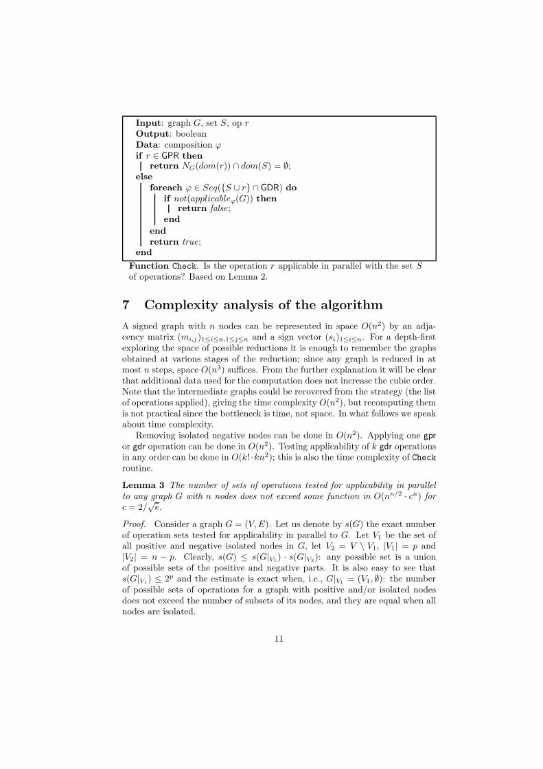
Input: graph G, set S, op rOutput: booleanData: composition ϕif r ∈ GPR then

return NG(dom(r)) ∩ dom(S) = ∅;else

foreach ϕ ∈ Seq({S ∪ r} ∩ GDR) doif not(applicableϕ(G)) then

return false;end

endreturn true;

end

Function Check. Is the operation r applicable in parallel with the set Sof operations? Based on Lemma 2.

7 Complexity analysis of the algorithm

A signed graph with n nodes can be represented in space O(n2) by an adja-cency matrix (mi,j)1≤i≤n,1≤j≤n and a sign vector (si)1≤i≤n. For a depth-firstexploring the space of possible reductions it is enough to remember the graphsobtained at various stages of the reduction; since any graph is reduced in atmost n steps, space O(n3) suffices. From the further explanation it will be clearthat additional data used for the computation does not increase the cubic order.Note that the intermediate graphs could be recovered from the strategy (the listof operations applied), giving the time complexity O(n2), but recomputing themis not practical since the bottleneck is time, not space. In what follows we speakabout time complexity.

Removing isolated negative nodes can be done in O(n2). Applying one gpr

or gdr operation can be done in O(n2). Testing applicability of k gdr operationsin any order can be done in O(k! ·kn2); this is also the time complexity of Checkroutine.

Lemma 3 The number of sets of operations tested for applicability in parallel

to any graph G with n nodes does not exceed some function in O(nn/2 · cn) for

c = 2/√

e.

Proof. Consider a graph G = (V, E). Let us denote by s(G) the exact numberof operation sets tested for applicability in parallel to G. Let V1 be the set ofall positive and negative isolated nodes in G, let V2 = V \ V1, |V1| = p and|V2| = n − p. Clearly, s(G) ≤ s(G|V1) · s(G|V2): any possible set is a unionof possible sets of the positive and negative parts. It is also easy to see thats(G|V1) ≤ 2p and the estimate is exact when, i.e., G|V1 = (V1, ∅): the numberof possible sets of operations for a graph with positive and/or isolated nodesdoes not exceed the number of subsets of its nodes, and they are equal when allnodes are isolated.

11

Now consider the rest of the graph, where only gdr operations may be ap-plied, with n′ = n − p nodes. The first operation can be chosen in at mostn′(n′ − 1)/2 ways, the i-th operation can be chosen in (n′ − 2i)(n′ − 2i− 1)/2

ways. This gives us at most Cn′

2,...,2,n′−2k = n′!(n′−2k)!2k sequences of pairs of nodes

chosen from n′ nodes. The corresponding number of sets is obtained ignoringthe order of pairs, i.e., dividing this number by k!. Since up to n/2 node pairscan be selected, the total estimate is

t(n′) =

n′/2∑

k=0

n′!

(n′ − 2k)!k!2k, (2)

and s(G|V2) ≤ t(n′). The latter is an equality, e.g., when V2 is complete.Notice that the last (k = ⌊n′/2⌋) term of t(n′) is equal to the product of odd

numbers not exceeding n′,

prodd(n′) = 1 · 3 . . . (2⌈n′/2⌉ − 1),

which alone grows faster than 2n′

. Thus, for sufficiently large n, for any graphG with n nodes, out of which p nodes are positive,

s(G) ≤ s(G|V1) · s(G|V2 ≤ 2p · t(n− p) ≤ t(n) = s(K−n ),

where K−n is a complete negative graph. Hence, it suffices to prove the lemma

for complete negative graphs.Let us rewrite (2) in the following way:

t(n′) =

n/2∑

k=0

n!

(n− 2k)!(2k)!· (2k)!

k!2k=

n/2∑

k=0

Cn2k · prodd(2k) ≤ 2n · prodd(2⌈n/2⌉).

From Stirling’s formula, we get n! = Θ(√

n(n/e)n). In case when n is even,t(n) ≤ 2n · prodd(n) and prodd(n) = n!

(n/2)!2n/2 ∈ O((n/e)n/2). In case when n

is odd, t(n) ≤ 2n ·prodd(n−1) and prodd(n−1) is also O((n/e)n/2). Therefore,t(n) ∈ O(nn/2 · (2/

√e)n), which proves the lemma. �

Lemma 4 The number of times the Complexity function is recursively called

does not exceed n! · 2n.

Proof. A sequential composition of operations can be written as a sequenceof nodes on which the operations are applied; the operations can be recoveredfrom the context. Therefore, the total number of possibilities is bounded by n!.

Unless two subsequent nodes correspond to a gdr operation, we might alsoneed to know if the associated operations are applied in the same step or not. Inthis way, there may be at most 2n−1 ways to partition a sequential compositionof operations into a parallel strategy. Hence, the total number of times we mayarrive to the empty graph does not exceed 1/2 · n! · 2n.

12

By a similar argument, the number of sub-strategies reducing k nodes is atmost 1/2 · n!/(n− k)! · 2k. Summing up over 0 ≤ k ≤ n,

n∑

k=0

1

2· n!

(n− k)!· 2k ≤ n! · 1

2

n∑

k=0

2k ≤ n! · 2n

. �

Theorem 1 The present algorithm is in O(

n2n+4

dn

)

for d = e2/√

8.

Proof. (sketch) The principal term of the algorithm’s complexity comes fromchecking the parallel applicability of different sets of operations for differentintermediate graphs by applying them in different order. This gives us the timecomplexity of O(⌊n/2⌋! · n3) ·O(nn/2 · cn)) ·O(n! · 2n) for c = 2/

√e. According

to Stirling’s formula for n!, n! ∈ Θ(√

n(n/e)n), so we can rewrite the timecomplexity of the algorithm as

O

(

nn/2 · n7/2

2n/2 · en/2· n

n/2 · 2n

en/2· n

n · n1/2 · 2n

en

)

.

Simplifying this expression, we obtain the estimate in the theorem statement.�

8 Heuristics

Instead of top-down recursive examination of the graph space one could considera bottom-up approach: compute the parallel complexity for all graphs of size k,from k = 0 to k = n− 1, by only examining one-step reductions and consultingthe complexity already computed for the smaller graphs. However, the numberof possible signed graphs of size n is 2n(n+1)/2, so the space requirements be-comes prohibitive as n grows. Even computing it only for the graphs obtainedin the reduction process of the given graph (caching) leads to hitting the spacebarrier before the time barrier.

Since the known complexity is so high, a natural question arises whetherheuristic algorithms can help. E.g., let us consider the Greedy approach: ex-amine only maximal sets of operations in each step of the reduction. In otherwords, we only consider reducing C(G) to C(G′) if G′ is obtained from G by aparallel application of the operations in set S, where no set S′ % S is applicablein parallel to G. Based on the same arguments used in analyzing the computa-tional complexity of our algorithm, it may be seen that this Greedy approachremains highly exponential, since it embeds the same three main levels of com-plexity discussed in Section 5. Regarding the output that the Greedy algorithmyields, in many example we have computed, this approach finds the optimum.However, one can see from the example in Figure 2 that, since operations gdr4,5

13

GFED@ABC1+ GFED@ABC2+ GFED@ABC3− GFED@ABC2+ GFED@ABC3−

GFED@ABC4− GFED@ABC5− GFED@ABC6+

GFED@ABC1+ GFED@ABC3−

GFED@ABC4− GFED@ABC5− GFED@ABC6+

Figure 3: Three options for the first step of a Greedy-type of reduction of thegraph G6 in Figure 2 (choose as many operations as possible); all three graphsare reducible in 3 steps, yielding 4 as a Greedy-computed parallel complexityfor G6, which is not optimal.

and gpr6 are applicable in parallel to G6, the Greedy approach does not examine{gdr4,5} because it is not a maximal set. The maximal sets are {gdr4,5, gpr6},{gpr1} and {gpr2}. It turns out that the optimal strategies are missed in thiscase, see Figure 3.

9 Software

An implementation of the algorithm can be found in [12]. In fact, this imple-mentation does not use recursion, but rather is done by backtracking, a non-recursive depth-first search of the strategy tree with cuts. The implementationin [12] also contains a heuristic, Greedy-style approach. In there only maximal(with respect to the number of operations, with operations considered in a fixedorder) sets are considered in every step of the algorithm. This variation is morethorough than Greedy algorithm as described in Section 8, but still it does notalways find an optimal strategy.

Acknowledgments A.A. gratefully acknowledges the support by Academy ofFinland, project 203667 and by the Science and Technology Center in Ukraine,project 4032. C.L. gratefully acknowledges the support by Academy of Fin-land, project 203667. I.P. gratefully acknowledges the support by Academy ofFinland, project 108421.

References

[1] A. Ehrenfeucht, T. Harju, I. Petre, D. M. Prescott, and G. Rozenberg. Formal systemsfor gene assembly in ciliates. Theoret. Comput. Sci. 292 (2003) 199–219.

[2] A. Ehrenfeucht, T. Harju, I. Petre, D. M. Prescott, G. Rozenberg. Computation in

Living Cells: Gene Assembly in Ciliates, Springer, 2003.

[3] A. Ehrenfeucht, D.M. Prescott, G. Rozenberg. Computational aspects of gene(un)scrambling in ciliates. In: L. F. Landweber, E. Winfree (eds.) Evolution as Compu-

tation. Springer, Berlin, Heidelberg, New York, 2001, 216-256.

[4] T. Harju, C. Li, I. Petre: Examples on the parallel complexity of signed graphs, submit-ted, 2007.

[5] T. Harju, C. Li, I. Petre, G. Rozenberg. Complexity Measures for Gene Assembly. In:K. Tuyls (Eds.), Proceedings of the Knowledge Discovery and Emergent Complexity in

Bioninformatics workshop. Springer, Lecture Notes in Bioinformatics 4366, 2007.

14

[6] T. Harju, C. Li, I. Petre, G. Rozenberg. Parallelism in gene assembly. Natural Computing

5 (2), Springer, 2006, 203–223.

[7] T. Harju, C. Li, I. Petre. Graph Theoretic Approach to Parallel Gene Assembly, 2007,submitted.

[8] T. Harju, I. Petre, G. Rozenberg. Gene assembly in ciliates: Formal frameworks. Bulletin

of EATCS 82, 2004, 227–241.

[9] C. L. Jahn, L. A. Klobutcher, Genome remodeling in ciliated protozoa. Ann. Rev.

Microbiol. 56, 2000, 489–520.

[10] L. F. Landweber, L. Kari. The evolution of cellular computing: Nature’s solution toa computational problem. In: Proceedings of the 4th DIMACS Meeting on DNA-Based

Computers, Philadelphia, PA, 1998, 3–15.

[11] L. F. Landweber, L. Kari. Universal molecular computation in ciliates. In: L. F. Landwe-ber and E. Winfree (eds.) Evolution as Computation, Springer, Berlin Heidelberg NewYork, 2002.

[12] I. Petre, S. Skogman. Gene Assembly Simulator, 2006.http://combio.abo.fi/simulator/ simulator.php.

[13] D. M. Prescott. The evolutionary scrambling and developmental unscrambling ofgermline genes in hypotrichous ciliates. Nucl. Acids Res. 27, 1999, 1243–1250.

[14] D.M. Prescott, A. Ehrenfeucht, G. Rozenberg. Molecular operations for DNA processingin hypotrichous ciliates. Europ. J. Protistology 37, 2001, 241260.

15