DEGREE PROJECT IN TECHNOLOGY, FIRST CYCLE, 15 CREDITS

STOCKHOLM, SWEDEN 2021

Graph Complexity Based on a

Heuristic That Involves the

Algorithmic Complexity Behaviour

of Multiplex Networks on Graphs

HASAN KALZI

KTH ROYAL INSTITUTE OF TECHNOLOGY

SCHOOL OF ELECTRICAL ENGINEERING AND COMPUTER SCIENCE

1

KTH Computer Science and Communication

Graph Complexity Based on a Heuristic That

Involves the Algorithmic Complexity

Behaviour of Multiplex Networks on Graphs

Hasan Kalzi

Kalzi@kth.se

Degree Project in Computer Science, DA150X

Examiner: Pawel Hermann

Supervisor: Arvind Kumar

Swedish title: Grafs Komplexitet Baserat på en Heuristik som Involverar Det

Algoritmiska Komplexitetsbeteendet hos Flernivånätverk på Grafer

DA150x Examensarbete inom datateknik, grundnivå

EECS/KTH 2021‐06-09

2

Graph Complexity Based on a

Heuristic That Involves the

Algorithmic Complexity Behaviour of

Multiplex Networks on Graphs

Abstract

Since determining the complexity of multiplex networks is an NP-hard

problem, I decided to calculate the complexity of graphs using heuristics. I

am the first in this path who did these kinds of calculations. I always wanted

to define complexity as a mathematical characteristic in the structure of

graphs. This investigation explores the behaviour of the algorithmic

complexity of multiplex networks on graphs to discover if it is possible to

extract a mathematical expression that can represent it. If we obtain a

mathematical representation for graph complexity, we tackle this problem

from the NP-hard problem area. It also can be used as one of the

characteristics of the graph, e.g., the number of nodes, edges, or motifs of

a specific size. Santoro and Nicosia, in their research, obtained the

algorithmic complexity of multiplex networks is defined [1]. Thus, an

approach that uses a heuristic strategy can be the easiest way to get near an

optimal mathematical definition of the complexity of graphs. In this thesis,

I re-introduce the recent representation of the algorithmic complexity [2]

for multiplex networks from an algorithmic information theory [ 3 ]

perspective. This definition depends mainly on Kolmogorov complexity [4,

5]. I studied the results of algorithmic complexity heuristic measurements

on different and random networks that differ in size-4 motifs number.

I found impressive results that show a logarithmic trend line (or maybe

power trend line) for the algorithmic complexity with increasing the

number of layers. Also, the algorithmic complexity decreases when the

number of motifs increases. Thus, there can be a mathematical connection

between the algorithmic complexity, the number of motifs, the number of

layers, the number of edges and the number of nodes. Furthermore, more

research is required to investigate and invent a mathematical expression

between these characteristics. Also, more research is needed to assert the

correctness of these conclusions on other kinds of networks with different

motifs size.

3

Grafs Komplexitet Baserat på en

Heuristik som Involverar Det

Algoritmiska Komplexitetsbeteendet

hos Flernivånätverk på Grafer

Sammanfattning

Eftersom problemet med att bestämma komplexiteten hos flerfaldiga

nätverk är ett NP-svårt problem, bestämde jag mig för att beräkna

komplexiteten hos grafer med hjälp av heuristik. Jag är den första på den

här vägen som gjorde den här typen av beräkningar. Jag ville alltid definiera

komplexitet som en matematisk egenskap i diagramstrukturen. Denna

uppsats undersöker beteendet hos den algoritmiska komplexiteten av

flerfaldiga nätverk i grafer för att upptäcka om det är möjligt att extrahera

ett matematiskt uttryck som kan representera det. Om vi får en matematisk

representation för grafkomplexitet, hanterar vi detta problem från det NP-

hårda problemområdet. Den kan också användas som en av diagrammets

egenskaper, såsom antalet noder, kanter eller motiv av en viss storlek. Den

algoritmiska komplexiteten av flerfaldiga nätverk definieras av Santoro

och Nicosia i deras forskningspapper [1]. Således kan ett tillvägagångssätt

som använder en heuristisk strategi vara det enklaste sättet att komma nära

en optimal matematisk definition av komplexiteten i grafer. I denna

avhandling introducerar jag den senaste representationen av den

algoritmiska komplexiteten [2] för flerfaldiga nätverk ur ett algoritmiskt

perspektiv för informationsteori [3]. Denna definition beror främst på

Kolmogorov-komplexiteten [4, 5 ]. Jag studerade resultaten av de

heuristiska algoritmiska komplexitetsmätningarna på olika och

slumpmässiga nätverk som skiljer sig åt i storlek-4-motivnummer.

Jag hittade imponerande resultat som visar en logaritmisk trendlinje (eller

kanske krafttrendlinje) för den algoritmiska komplexiteten med att öka

antalet lager. Den algoritmiska komplexiteten minskar också när antalet

motiv ökar. Således kan det finnas en matematisk koppling mellan den

algoritmiska komplexiteten, antalet motiv, antalet lager, antalet kanter och

antalet noder. Dessutom krävs mer forskning för att undersöka och

uppfinna ett matematiskt uttryck mellan dessa egenskaper. Dessutom

behövs mer forskning för att hävda riktigheten av dessa slutsatser på andra

olika typer av nätverk.

4

Table of contents

List of Figures 6

Acknowledgements 6

1. Introduction 7

1.1. Problem Statement 8

1.2. Purpose 8

1.3. Scope 9

1.4. Approach 9

1.5. Thesis Outline 10

2. Background 11

2.1. Graph 11

2.1.1. Undirected- and Directed-Graphs 11

2.1.2. Weighted- and Unweighted-Graphs 13

2.2. Systems or Networks 13

2.2.1. Network Motif 15

2.3. Complex Systems 16

2.3.2. Multiplex Networks 20

2.3.3. The Aggregated Single-Layer Multiplex Network 22

2.4. The Complexity 23

2.4.1. Kolmogorov Complexity or Algorithmic Complexity 23

2.4.1.1. Calculating Algorithmic Complexity 24

2.4.2. The Complexity of Graphs Regarding the Mathematical

Theory of Randomness Perspective 25

2.4.3. The Algorithmic Complexity of Multiplex Networks 26

2.4.3.1. Encoding Multiplexes 28

3. Method 29

3.1. The Used Datasets 29

3.2. The Algorithmic Complexity of Graphs 30

3.2.1. The Optimisation of The Datasets 31

3.2.2. Randomising Graphs 31

3.2.3. Calculating Algorithmic Complexity of Graphs 32

4. Results 33

5

4.1. 1st dataset 𝑁=100, e ≈ 1000 33

4.1.1. The Algorithmic Complexity Behaviour 35

4.2. 2nd dataset 𝑁=200, e ≈ 3800 37

4.2.1. The Algorithmic Complexity Behaviour 39

5. Discussion 41

5.1. The quality of 𝐶(𝑀) 41

5.2. The quality of heuristics and heuristic results 42

6. Conclusion 43

Further research 43

7. Appendices 44

Appendix A Prime-Weight Matrix Encoding 44

Appendix B Detailed Results 45

N = 100, e = 986 45

N = 200, e = 3800 55

8. References 59

1

6

List of Figures

[F1] Networking: Building Your Contacts in New, More Effective Ways

https://insights.dice.com/2019/09/25/networking-building-contacts-

effective/

[F3] Table 1 A list of the real-world complex networks that will be

studied, Vito Latora, Vincenzo Nicosia, Giovanni Russo, Complex

Networks: Principles, Methods and Applications,

https://www.cambridge.org/se/academic/subjects/physics/statistical-

physics/complex-networks-principles-methods-and-

applications?format=HB&isbn=9781107103184 (Cambridge University

Press, 2017)

[F2] DATA SET 4: The Neural Network of the C. elegans, Vito Latora,

Vincenzo Nicosia, Giovanni Russo, Complex Networks: Principles,

Methods and Applications,

https://www.cambridge.org/se/academic/subjects/physics/statistical-

physics/complex-networks-principles-methods-and-

applications?format=HB&isbn=9781107103184 (Cambridge University

Press, 2017)

[F4] SL: Storstockholms Lokaltrafik official web page,

https://mitt.sl.se/reseplanering/tidtabeller#/TimeTableSearch/GetLineTim

eTables/NULL/NULL/NULL/METRO/35/0/10

[F5] SL: Storstockholms Lokaltrafik official web page,

https://tunnelbanakarta.se/wp-content/uploads/2019/10/tunnelbana-

stockholm.jpg

[F6] Andrea Santoro and Vincenzo Nicosia, Algorithmic Complexity of

Multiplex Networks,

https://journals.aps.org/prx/abstract/10.1103/PhysRevX.10.021069

Acknowledgements

The author thanks PhD Student Andrea Santoro and PhD Vincenzo

Nicosia for helpful conversations and lectures about algorithmic

complexity.

The author thanks Anna Skantz and Solbritt Gateman for providing this

search with a set of graphs that has a different number of motifs.

7

Chapter 1

1. Introduction

We say that the universe is complex but, what does that mean? What do we

mean by more/less complicated when we compare things? When we hear

the word complexity, the first thought is a formation, or a circumstance

formed of many parts or difficult to understand. Complexity has not a

unique definition. The definition varies and depends on the problem.

Multiplicity and diversity are the common characteristics that characterise

the definition of complexity. The graphs are mathematical structures used

to model pairwise relations between objects [3]. Nowadays, the NP-hard

problem of determining the complexity of graphs and set a reasonable

expression describing it eludes scientists. The most existing approaches

came from, for example, graph theory which is the study of graphs. These

approaches can occasionally only handle a single graph's feature but not a

complete characterisation of the graph's properties. Some of these measures

introduce new information which does not present in the original ones.

Besides, most of them discard valuable information either by

overestimating or underestimating graph properties. Thus, developing a

near-optimal complexity calculating method using traditional approaches

is very difficult, so we need an alternative approach with a more effective

strategy to calculate the complexity of networks more precisely.

We know that every object consists of elements or particles that connect in

specific ways. We can represent any object in graphs. In these graphs, the

vertices are the elements (e.g., atoms, cells, bus stops or humans), while the

edges bind these elements. These edges are responsible for the emergence

of complex dynamical behaviours. These objects can connect and form

systems (such as a transportation network or the human body). Thus, a

single graph or groups of graphs can connect and work together to build

complex networks [6]. Complex networks are the foundation of complex

systems, from the human brain to computer communications, from

transport infrastructures to financial markets [6].

The multilayer network representation [ 7 ] of a complex system can

preserve complete information about the different interactions among the

constituents of a complex system. This representation has recently proven

truly useful in modelling transportation networks, social circles, the human

brain, and many more. A Santoro and V Nicosia [1] concluded that the

algorithmic complexity judge which one is the better multilayer

8

representation among many multilayer representations of complex

networks. They also used this definition of complexity in the redundancy

problem by reducing the number of layers that not adding more information

to a multilayer representation. Thus, it is vital to study this definition of

complexity and study its characteristics on different networks.

1.1. Problem Statement

Nowadays, networks have an essential role in life and studies. I believe that

networks will be even more vital in future discoveries and more

complicated constructed networks. Until today, there is no clear scientific

definition of the complexity of networks which means that there is no

mathematical expression or table to calculate it. We always know that

complexity exists. I want concrete and beneficial representation for the

complexity of networks to discover how the complexity connects with all

network components (edges, nodes, redundancy, and motifs) to tackle this

problem out of the range of the NP-hard problem area. A Santoro and V

Nicosia used this definition of complexity to determine which

representation is truly multiplex representation (i.e., the higher the

complexity is, the better is the multiplex representation) by comparing the

corresponding values of algorithmic complexity for different networks [1].

This definition of algorithmic complexity is also can be used to:

• Obtain low-dimensional delineations of multi-dimensional systems

[1].

• Cluster multilayer networks into a small set of meaningful

superfamilies [1].

• Detect tipping points in the evolution of different time-varying

multilayer graphs [1,8].

Thus, I found this definition is quite interesting, so I chose to re-introduce

the algorithmic complexity from A Santoro and V Nicosia research report

among all graph complexity definitions and study its behaviour on different

networks.

1.2. Purpose

This thesis presents the algorithmic complexity of multiplex networks and

investigates the algorithmic complexity behaviour on specific types of

9

networks heuristically to draw mathematical characteristics of the

complexity of graphs.

Regarding algorithmic information theory [2], I have two subjects in focus.

The first is the definition of network complexity of complex networks. The

second is finding a method that depends on this definition to measure the

complexity of graphs. With this in mind, I pose the following questions:

• What is the algorithmic complexity of multiplex networks?

• What does this complexity indicate? Can we obtain a

mathematical expression that allows us to use it as the complexity

of graphs (all graphs generally)?

1.3. Scope

This thesis only focuses on the definition of the algorithmic complexity of

multiplex networks [1] (which takes into consideration directed and

unweighted networks). This thesis only focuses on the definition of the

algorithmic complexity of multiplex networks. Thus, I focused primarily

to evaluate the algorithmic complexity of unweighted, directed networks. I

studied the algorithmic complexity behaviour on networks that has the

following characters:

• Exactly 100 nodes, about 1000 edges and the number of motifs of size

4 varies between 50 000 and 300 000.

• Exactly 200 nodes, about 4000 edges and the number of motifs of size

4 varies between 3 000 000 and 3 400 000.

1.4. Approach

This thesis will primarily evaluate the different values of the algorithmic

complexity on networks represented in an aggregated single-layered graph.

Santoro and Nicosia [1] defined the algorithmic complexity after the ratio

of the Kolmogorov complexity 𝑲𝑪(𝑺) [3, 7] of the bit strings associated

with the multilayer and to the corresponding aggregated graph. The

Kolmogorov complexity 𝑲𝑪(𝑺) of a bit string 𝑺 is defined as the length of

the shortest computer program that generates 𝑺 as output [5,8]. I evaluate

this method on different networks to investigate the behaviour of the

algorithmic complexity heuristically. I did this by distributing the network

10

into 𝑴 random layers and calculate the complexity 𝑪(𝑴) of this

corresponding representation regarding the definition above.

Kolmogorov complexity is not computable [ 9 ]. Andrea Santoro and

Vincenzo Nicosia introduced a sensible approach to calculate it. This

approach takes into consideration the initial object (𝑀) then compress this

object (more specific, the bit string that represents) with any compress

algorithm (Gzip [10]). The upper bound for Kolmogorov complexity of

𝑀 will be the concatenation of the output of the compression algorithm plus

the compression algorithm itself. I can run these two things on a Turing

machine and obtain back the object.

1.5. Thesis Outline

• In the 2nd chapter, the reader will be introduced to the principles

behind the problem.

• All methods and the tools used to obtain credible results will be

explained and motivated in the 3rd chapter. All assumptions that are

made and the test data that will be used are addressed here.

• The results that I obtained will be presented in the 4th chapter. These

results are then interpreted and discussed in the following section.

• In the 6th section, I draw the conclusions for the problem statement

are made based on the prior discussion.

• The 7th chapter includes suggestion the appendices.

• Finally, all the references used in the thesis are listed in the final

section.

11

Chapter 2

2. Background

To invent a good strategy for defining the complexity of graphs and study

the behaviour of algorithmic complexity of graphs on specific types of

networks, we must know about complexity, graphs, networks, multiplex

networks, and network motifs. In this section, I will explain all the

mentioned terms. Subsequently, I will present and describe the

Kolmogorov complexity and the complexity of multiplex networks.

2.1. Graph

In this thesis, I am interested in studying the complexity behaviour on

unweighted and directed graphs.

According to discrete mathematics [11], a graph consists of nodes or

vertices (singular: vertex) and edges that connect those nodes in a specific

way. There are two primary properties in graphs:

1. Directed or undirected graphs.

2. Weighted or unweighted graphs.

2.1.1. Undirected- and Directed-Graphs

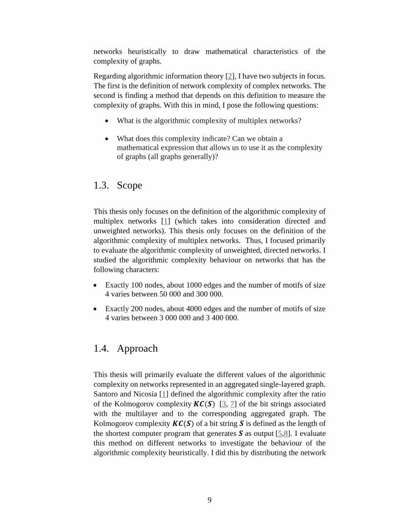
A graph is undirected when two nodes are connected in both ways. For

example, in figure 2.1a, we can go from node 1 to node 2 and oppositely.

We can represent the edges by writing edge A to edge B, or the opposite,

as shown in figure 2.1b. A real-world example of undirected graphs is

moving between metro stations in Stockholm using the same ticket. This

ticket can take you wherever you want to go in both ways, and that is why

we do not care about the direction.

12

Figure (2.1)

(a) An example of undirected graphs the nodes are (b) The edges representation for the graph

numbered from 0 to 5.

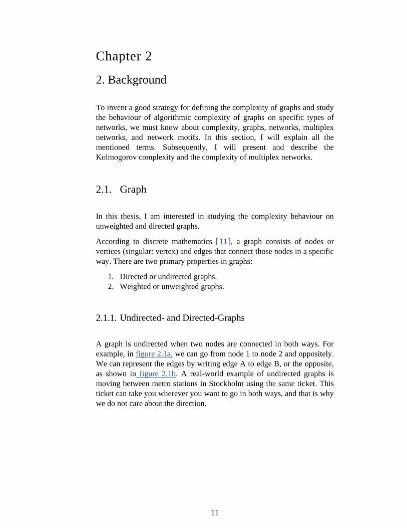
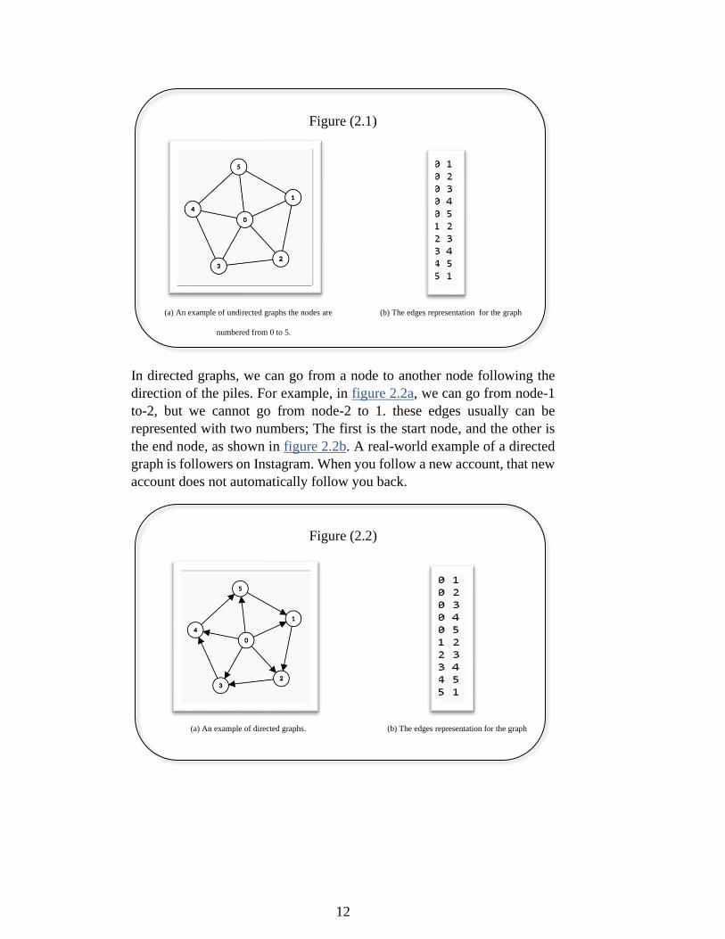
In directed graphs, we can go from a node to another node following the

direction of the piles. For example, in figure 2.2a, we can go from node-1

to-2, but we cannot go from node-2 to 1. these edges usually can be

represented with two numbers; The first is the start node, and the other is

the end node, as shown in figure 2.2b. A real-world example of a directed

graph is followers on Instagram. When you follow a new account, that new

account does not automatically follow you back.

Figure (2.2)

(a) An example of directed graphs. (b) The edges representation for the graph

13

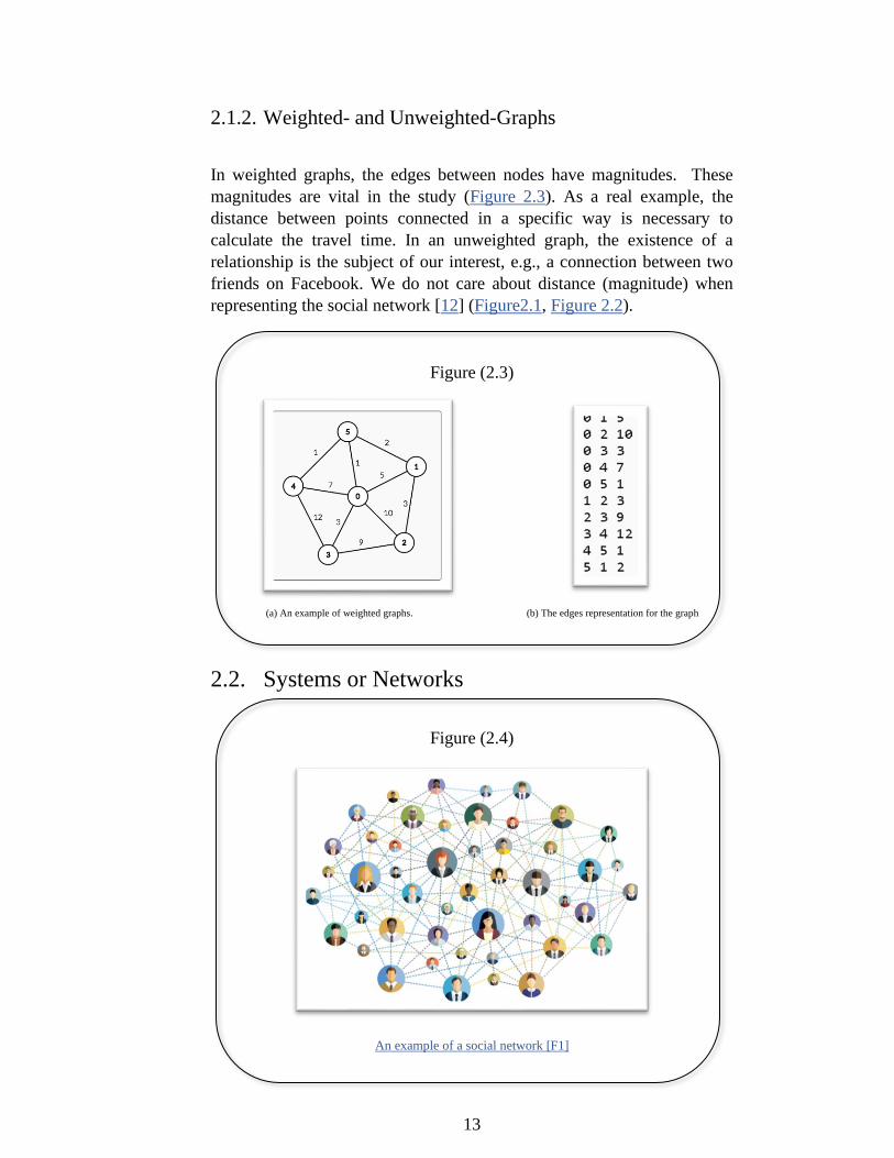
2.1.2. Weighted- and Unweighted-Graphs

In weighted graphs, the edges between nodes have magnitudes. These

magnitudes are vital in the study (Figure 2.3). As a real example, the

distance between points connected in a specific way is necessary to

calculate the travel time. In an unweighted graph, the existence of a

relationship is the subject of our interest, e.g., a connection between two

friends on Facebook. We do not care about distance (magnitude) when

representing the social network [12] (Figure2.1, Figure 2.2).

Figure (2.3)

(a) An example of weighted graphs. (b) The edges representation for the graph

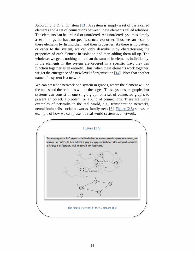
2.2. Systems or Networks

Figure (2.4)

An example of a social network [F1]

14

According to D. S. Ornstein [13], A system is simply a set of parts called

elements and a set of connections between these elements called relations.

The elements can be ordered or unordered. An unordered system is simply

a set of things that have no specific structure or order. Thus, we can describe

these elements by listing them and their properties. As there is no pattern

or order to the system, we can only describe it by characterising the

properties of each element in isolation and then adding them all up. The

whole set we get is nothing more than the sum of its elements individually.

If the elements in the system are ordered in a specific way, they can

function together as an entirety. Thus, when these elements work together,

we get the emergence of a new level of organisation [14]. Note that another

name of a system is a network.

We can present a network or a system in graphs, where the element will be

the nodes and the relations will be the edges. Thus, systems are graphs, but

systems can consist of one single graph or a set of connected graphs to

present an object, a problem, or a kind of connections. There are many

examples of networks in the real world, e.g., transportation networks,

neural brain cells, social networks, family trees [6]. Figure (2,5) shows an

example of how we can present a real-world system as a network.

Figure (2.5)

The Neural Network of the C. elegans [F2]

15

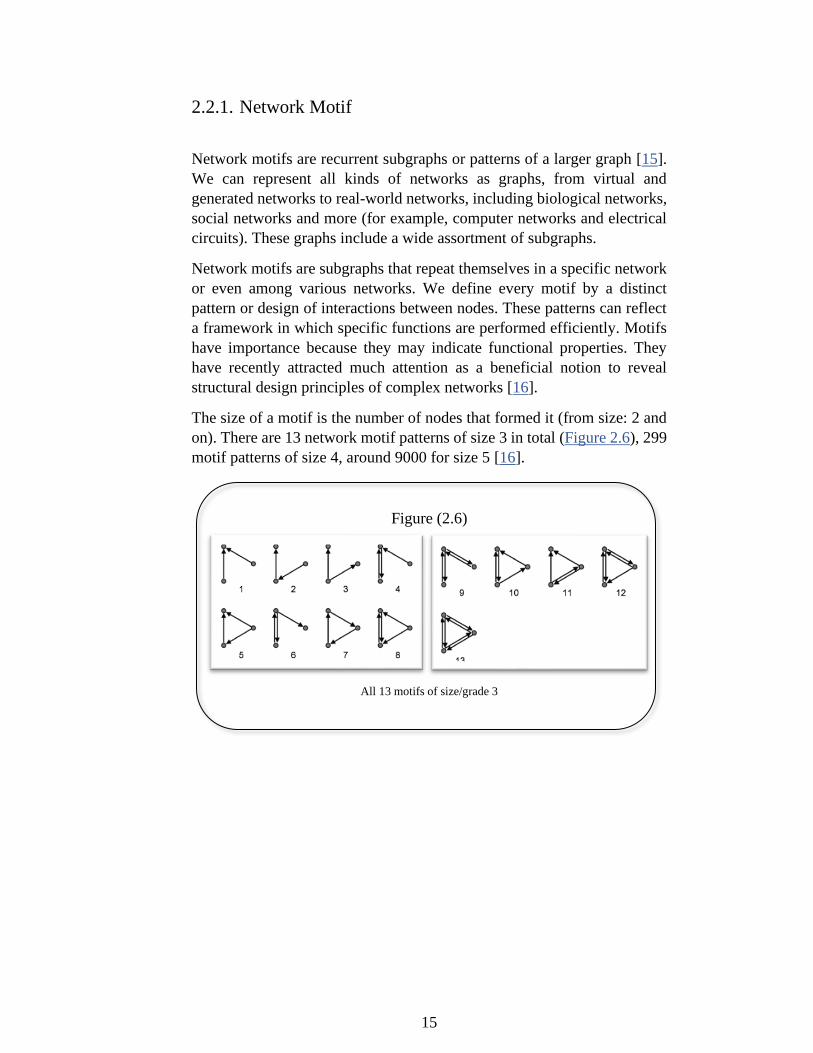
2.2.1. Network Motif

Network motifs are recurrent subgraphs or patterns of a larger graph [15].

We can represent all kinds of networks as graphs, from virtual and

generated networks to real-world networks, including biological networks,

social networks and more (for example, computer networks and electrical

circuits). These graphs include a wide assortment of subgraphs.

Network motifs are subgraphs that repeat themselves in a specific network

or even among various networks. We define every motif by a distinct

pattern or design of interactions between nodes. These patterns can reflect

a framework in which specific functions are performed efficiently. Motifs

have importance because they may indicate functional properties. They

have recently attracted much attention as a beneficial notion to reveal

structural design principles of complex networks [16].

The size of a motif is the number of nodes that formed it (from size: 2 and

on). There are 13 network motif patterns of size 3 in total (Figure 2.6), 299

motif patterns of size 4, around 9000 for size 5 [16].

Figure (2.6)

All 13 motifs of size/grade 3

16

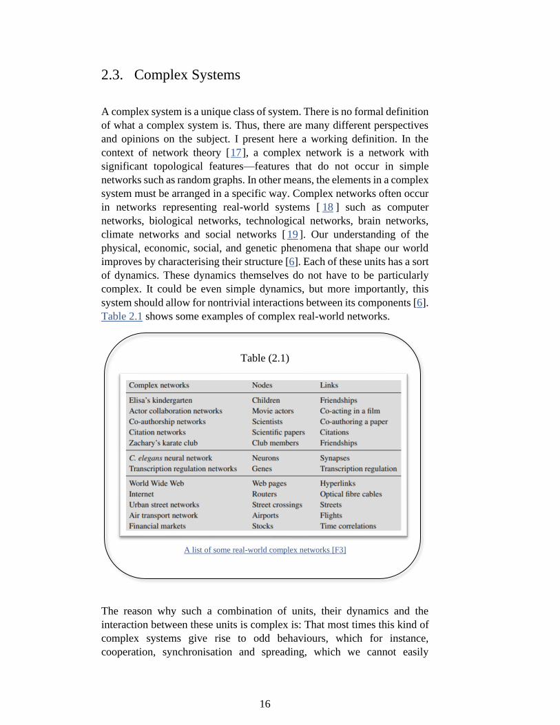
2.3. Complex Systems

A complex system is a unique class of system. There is no formal definition

of what a complex system is. Thus, there are many different perspectives

and opinions on the subject. I present here a working definition. In the

context of network theory [17], a complex network is a network with

significant topological features—features that do not occur in simple

networks such as random graphs. In other means, the elements in a complex

system must be arranged in a specific way. Complex networks often occur

in networks representing real-world systems [ 18 ] such as computer

networks, biological networks, technological networks, brain networks,

climate networks and social networks [ 19 ]. Our understanding of the

physical, economic, social, and genetic phenomena that shape our world

improves by characterising their structure [6]. Each of these units has a sort

of dynamics. These dynamics themselves do not have to be particularly

complex. It could be even simple dynamics, but more importantly, this

system should allow for nontrivial interactions between its components [6].

Table 2.1 shows some examples of complex real-world networks.

Table (2.1)

A list of some real-world complex networks [F3]

The reason why such a combination of units, their dynamics and the

interaction between these units is complex is: That most times this kind of

complex systems give rise to odd behaviours, which for instance,

cooperation, synchronisation and spreading, which we cannot easily

17

attribute them to just single unit, just single dynamics or just interruptions.

The combination of these three ingredients is responsible for the emergence

of these fascinating behaviours. Odd in this sequence means something that

is not trivial [1, 19].

By adding complexity to the system principle, we get a new system with

new properties. Some of these properties can be numerosity, redundancy,

interdependence, connectivity, and adaption. The only property that

probably exists in all definitions of a complex system is numerosity.

Numerosity means that the system consists of many parts that distributed

out without centralised control. An organisation is formed out of the local

interactions between the segments through a self-organisation process. This

process gives rise to the emergence of new levels of organisations. With

the phenomena of emergence that we described previously, the system will

develop into a whole new level [20, 21, 22]. When the system starts to

interact with other systems in its environment, we get new patterns of

organisation as results. Once again, we get the emergence of another level

of organisation. We talk about the number of elements and different levels

of the hierarchy within the system. For example, people form part of social

groups that form part of broader society. This wider society forms part of

humanity in turns. The complex systems have hierarchal structures, where

the elements are nested in subsystems that form part of a more

comprehensive system in turn. All complex systems have this multi-

dimensional property that composed of many components on many

different scales. Each scale is interconnected and interdependent with the

others. Thus, we cannot completely isolate one element or reduce the whole

system to one level (aggregated single layer). That means the complex

system must be presented in layers (or some other way) to preserve its data

(or information). I only focus on numerosity since we can represent it in a

multiplex network (we can call it multi-level or multi-layered) because it is

directly connected to the algorithmic complexity of multiplex networks

[20, 21, 22].

According to the hypotheses of complex networks, if we look at the

interactions among the units of a complex system, we can still recover most

of the essential information about the system's function [19]. There is a long

wave of literature on studying complex networks in this sense. These

studies are tying up the system's complexity with the complexity of the

scaffolding of the interaction network among its elements. One of the most

recent developments in this direction is the multiplex metaphor [23] which

helps to describe the numerosity property in a complex system by

representing it in a multiplex network.

18

2.3.1. The Multiplex Metaphor

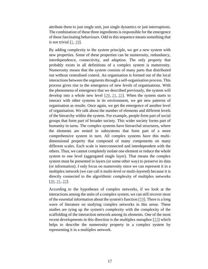
In complex systems, numerosity can generate redundancy. A basic and

simple example is human societies. The units or the nodes are people, and

they can interact in several different ways. They can be friends on Facebook

or any other social network, family interactions, collaboration, or simply

old-style friendships, as shown in figure 2.7. There are several thousand

different ways we can communicate today. In figure 2.7, we can see person

P connects with a friend F in all the social media networks represented in

the figure. Repeating the same edge in a simple graph will produce

redundancy [23]. The multiplex metaphor can solve this problem.

A metaphor describes an object or action in such a way that is not always

true but can help explain an idea or make a comparison [24]. We can also

say that a metaphor states one thing into another thing. In a multiplex

metaphor, for each interaction of the complex system, we try to disentangle

all the possible ways of two elements can be connected (or interrupted)

(Figure 2.8). We do not forget that we presented these entities as nodes.

19

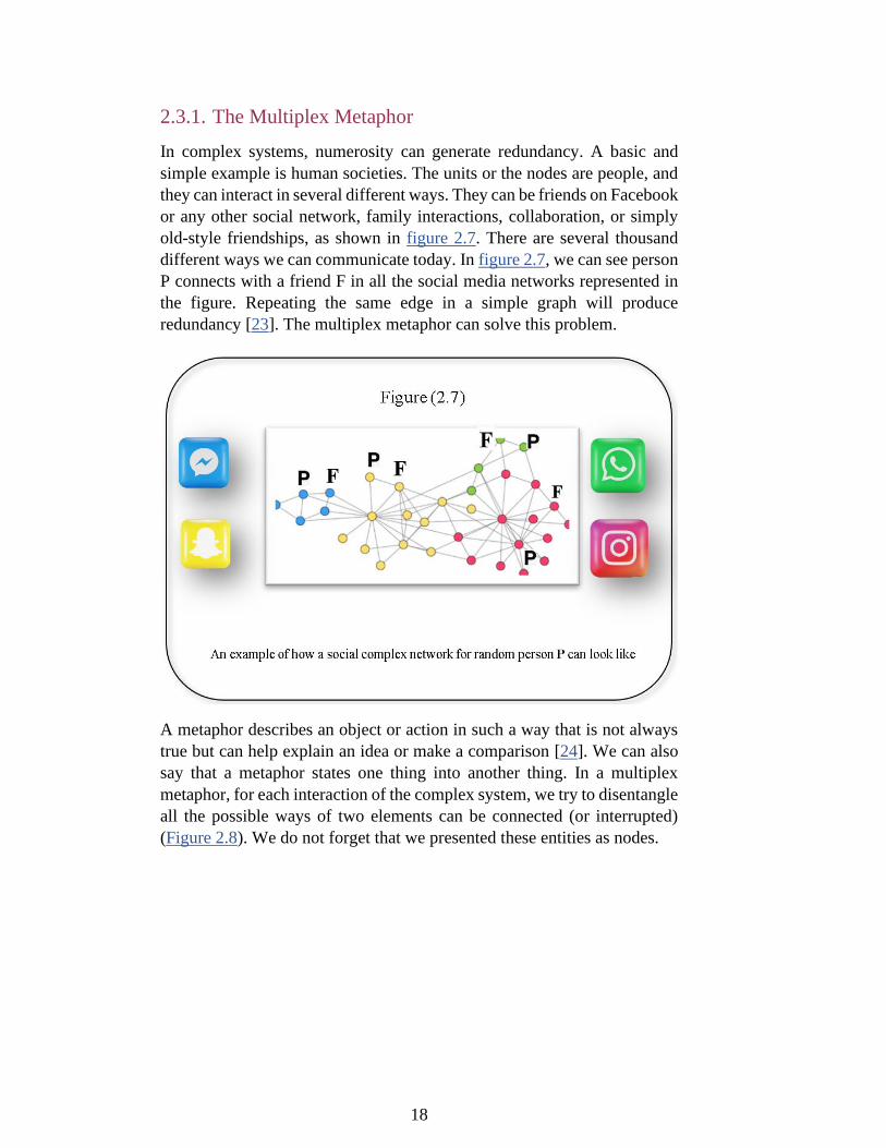
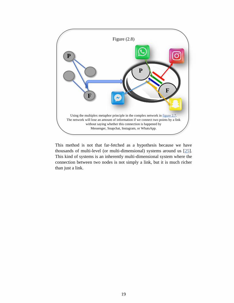
Figure (2.8)

Using the multiplex metaphor principle in the complex network in figure 2.7.

The network will lose an amount of information if we connect two points by a link

without saying whether this connection is happened by

Messenger, Snapchat, Instagram, or WhatsApp.

This method is not that far-fetched as a hypothesis because we have

thousands of multi-level (or multi-dimensional) systems around us [25].

This kind of systems is an inherently multi-dimensional system where the

connection between two nodes is not simply a link, but it is much richer

than just a link.

P

F

P

F

20

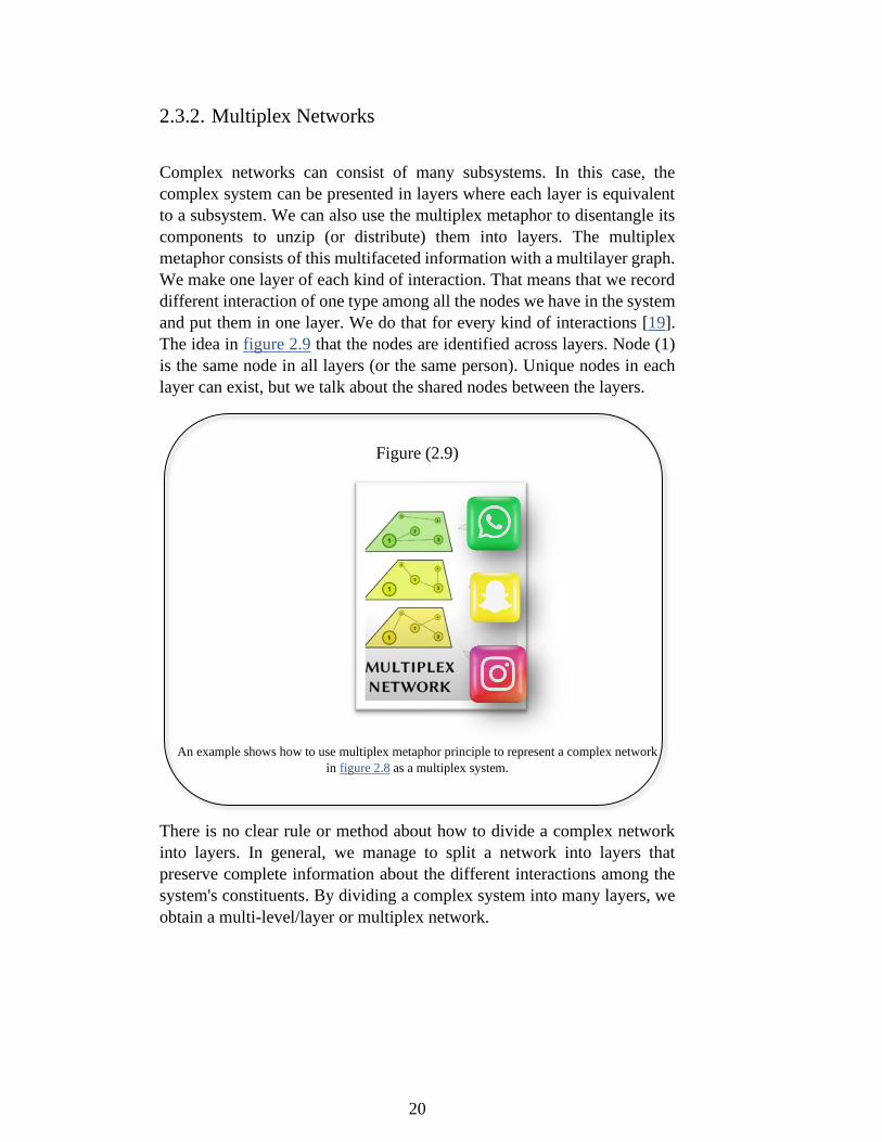
2.3.2. Multiplex Networks

Complex networks can consist of many subsystems. In this case, the

complex system can be presented in layers where each layer is equivalent

to a subsystem. We can also use the multiplex metaphor to disentangle its

components to unzip (or distribute) them into layers. The multiplex

metaphor consists of this multifaceted information with a multilayer graph.

We make one layer of each kind of interaction. That means that we record

different interaction of one type among all the nodes we have in the system

and put them in one layer. We do that for every kind of interactions [19].

The idea in figure 2.9 that the nodes are identified across layers. Node (1)

is the same node in all layers (or the same person). Unique nodes in each

layer can exist, but we talk about the shared nodes between the layers.

Figure (2.9)

An example shows how to use multiplex metaphor principle to represent a complex network

in figure 2.8 as a multiplex system.

There is no clear rule or method about how to divide a complex network

into layers. In general, we manage to split a network into layers that

preserve complete information about the different interactions among the

system's constituents. By dividing a complex system into many layers, we

obtain a multi-level/layer or multiplex network.

21

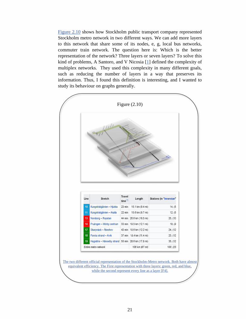
Figure 2.10 shows how Stockholm public transport company represented

Stockholm metro network in two different ways. We can add more layers

to this network that share some of its nodes, e, g, local bus networks,

commuter train network. The question here is: Which is the better

representation of the network? Three layers or seven layers? To solve this

kind of problems, A Santoro, and V Nicosia [1] defined the complexity of

multiplex networks. They used this complexity in many different goals,

such as reducing the number of layers in a way that preserves its

information. Thus, I found this definition is interesting, and I wanted to

study its behaviour on graphs generally.

Figure (2.10)

The two different official representation of the Stockholm-Metro network. Both have almost

equivalent efficiency. The First representation with three layers: green, red, and blue,

while the second represent every line as a layer [F4].

22

2.3.3. The Aggregated Single-Layer Multiplex Network

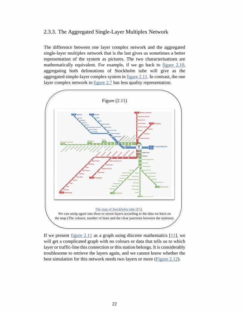
The difference between one layer complex network and the aggregated

single-layer multiplex network that is the last gives us sometimes a better

representation of the system as pictures. The two characterisations are

mathematically equivalent. For example, if we go back to figure 2.10,

aggregating both delineations of Stockholm tube will give as the

aggregated simple-layer complex system in figure 2.11. In contrast, the one

layer complex network in figure 2.7 has less quality representation.

Figure (2.11)

The map of Stockholm tube [F5].

We can unzip again into three or seven layers according to the data we have on

the map (The colours, number of lines and the clear junctions between the stations).

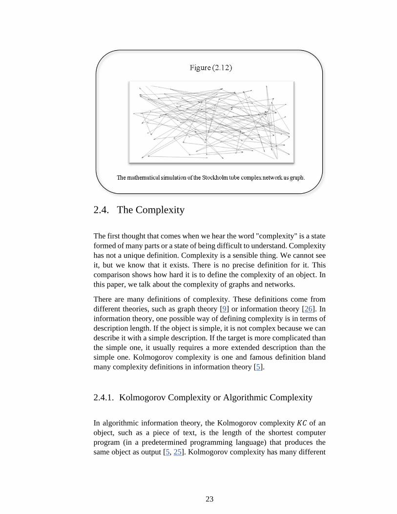
If we present figure 2.11 as a graph using discrete mathematics [11], we

will get a complicated graph with no colours or data that tells us to which

layer or traffic-line this connection or this station belongs. It is considerably

troublesome to retrieve the layers again, and we cannot know whether the

best simulation for this network needs two layers or more (Figure 2.12).

23

2.4. The Complexity

The first thought that comes when we hear the word "complexity" is a state

formed of many parts or a state of being difficult to understand. Complexity

has not a unique definition. Complexity is a sensible thing. We cannot see

it, but we know that it exists. There is no precise definition for it. This

comparison shows how hard it is to define the complexity of an object. In

this paper, we talk about the complexity of graphs and networks.

There are many definitions of complexity. These definitions come from

different theories, such as graph theory [9] or information theory [26]. In

information theory, one possible way of defining complexity is in terms of

description length. If the object is simple, it is not complex because we can

describe it with a simple description. If the target is more complicated than

the simple one, it usually requires a more extended description than the

simple one. Kolmogorov complexity is one and famous definition bland

many complexity definitions in information theory [5].

2.4.1. Kolmogorov Complexity or Algorithmic Complexity

In algorithmic information theory, the Kolmogorov complexity 𝐾𝐶 of an

object, such as a piece of text, is the length of the shortest computer

program (in a predetermined programming language) that produces the

same object as output [5, 25]. Kolmogorov complexity has many different

24

names, e.g., algorithmic complexity, program-size complexity, descriptive

complexity.

The algorithmic complexity of any object is the shortest program for a

touring machine that can generate it as an output. An example, Consider

the following two strings of 32 lowercase letters and digits:

• azazazazazazazazazazazazazazazaz

• 4c1j5b2p0cv4w1x8rx2y39umgw5q85s7

The first string has a short English-language description. Namely (write az

16 times) that consists of 17 characters. The second one has no simple

description (using the same character set) other than writing down the

whole string itself, i.e., (write 4c1j5b2p0cv4w1x8rx2y39umgw5q85s7)

that has 38 characters. The writing operation of the first string can be said

to have less complexity than writing the second because the first expression

is shorter than the other one.

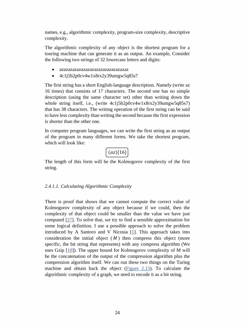
In computer program languages, we can write the first string as an output

of the program in many different forms. We take the shortest program,

which will look like:

(𝑎𝑧){16}

The length of this form will be the Kolmogorov complexity of the first

string.

2.4.1.1. Calculating Algorithmic Complexity

There is proof that shows that we cannot compute the correct value of

Kolmogorov complexity of any object because if we could, then the

complexity of that object could be smaller than the value we have just

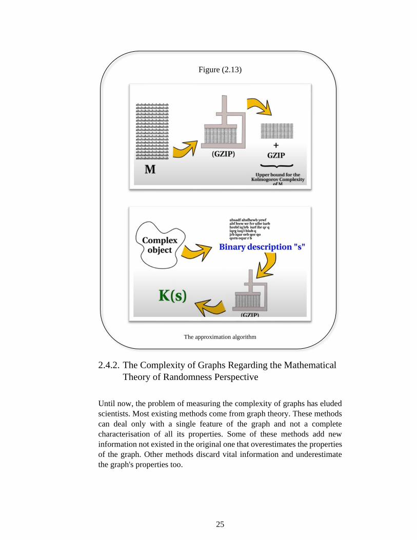
computed [27]. To solve that, we try to find a sensible approximation for

some logical definition. I use a possible approach to solve the problem

introduced by A Santoro and V Nicosia [1]. This approach takes into

consideration the initial object ( 𝑀 ) then compress this object (more

specific, the bit string that represents) with any compress algorithm (We

uses Gzip [10]). The upper bound for Kolmogorov complexity of M will

be the concatenation of the output of the compression algorithm plus the

compression algorithm itself. We can run these two things on the Turing

machine and obtain back the object (Figure 2.13). To calculate the

algorithmic complexity of a graph, we need to encode it as a bit string.

25

Figure (2.13)

The approximation algorithm

2.4.2. The Complexity of Graphs Regarding the Mathematical

Theory of Randomness Perspective

Until now, the problem of measuring the complexity of graphs has eluded

scientists. Most existing methods come from graph theory. These methods

can deal only with a single feature of the graph and not a complete

characterisation of all its properties. Some of these methods add new

information not existed in the original one that overestimates the properties

of the graph. Other methods discard vital information and underestimate

the graph's properties too.

26

H. Zenil, N.A. Kiani and J. Tegnér, F. Soler-Toscano, K. Dingle and A.

Louis [20, 21, 22] introduced a robust method to measure graph complexity

based upon the accepted mathematical theory of randomness. This measure

of complexity uses algorithmic complexity. It also depends on the

probability of reproducing the graph by a random computer program as

output. According to the theory of randomness, a graph has low algorithmic

complexity if there many computer programs that can regenerate it as an

output because short computer programs are most likely to produce by

chance. Vice versa, a graph has high algorithmic complexity if there few

computer programs that can regenerate it as an output.

2.4.3. The Algorithmic Complexity of Multiplex Networks

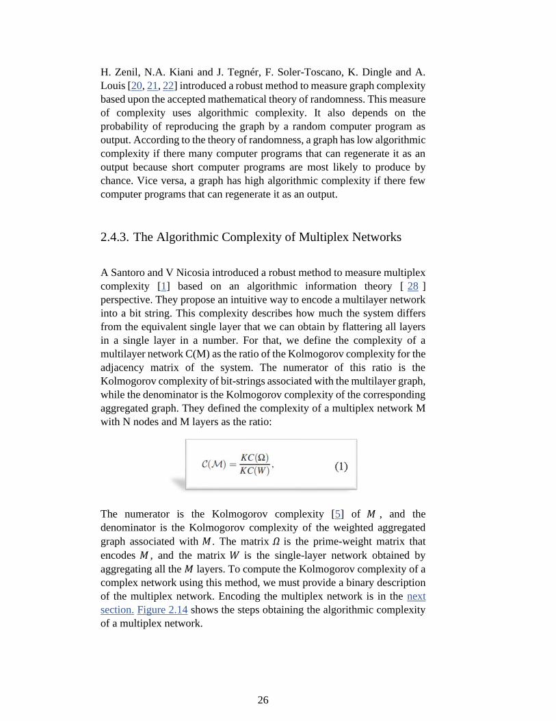
A Santoro and V Nicosia introduced a robust method to measure multiplex

complexity [1] based on an algorithmic information theory [ 28 ]

perspective. They propose an intuitive way to encode a multilayer network

into a bit string. This complexity describes how much the system differs

from the equivalent single layer that we can obtain by flattering all layers

in a single layer in a number. For that, we define the complexity of a

multilayer network C(M) as the ratio of the Kolmogorov complexity for the

adjacency matrix of the system. The numerator of this ratio is the

Kolmogorov complexity of bit-strings associated with the multilayer graph,

while the denominator is the Kolmogorov complexity of the corresponding

aggregated graph. They defined the complexity of a multiplex network M

with N nodes and M layers as the ratio:

The numerator is the Kolmogorov complexity [5] of 𝑀 , and the

denominator is the Kolmogorov complexity of the weighted aggregated

graph associated with 𝑀 . The matrix 𝛺 is the prime-weight matrix that

encodes 𝑀 , and the matrix 𝑊 is the single-layer network obtained by

aggregating all the 𝑀 layers. To compute the Kolmogorov complexity of a

complex network using this method, we must provide a binary description

of the multiplex network. Encoding the multiplex network is in the next

section. Figure 2.14 shows the steps obtaining the algorithmic complexity

of a multiplex network.

27

This quantity normally larger than one 𝐶(𝑀) >= 1 because if we have

more layers, we will have more primes in the encoding which leads to This

quantity usually larger than one (𝐶(𝑀) >= 1) because if the more layers

the multiplex has, the more primes the encoding will produce, which leads

to longer strings. Higher complexity means more correlative data contained

in the multiplex version of the complex system than the information in the

corresponding aggregated one. As a particular case, 𝐶(𝑀) = 1 if the

multiplex network consists of 𝑀 identical layers. If 𝐶(𝑀) ≈ 1, it would

not make much difference to represent the multiplex as a single-layered

graph, since the multiplex representation is not adding much more

information. When 𝐶(𝑀) >> 1, we can have a proper multiplex model

so that the eventual aggregations of layers into a single-layer graph might

discard some vital structural information. For more details see A Santoro

and V Nicosia report [1, appendix B].

Figure (2.14)

The steps to obtain the complexity of a complex system that has 𝑀 layers [F6].

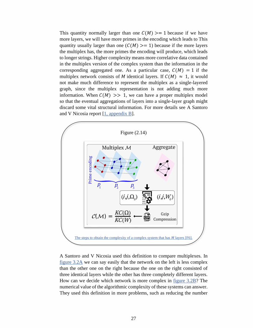
A Santoro and V Nicosia used this definition to compare multiplexes. In

figure 3.2A we can say easily that the network on the left is less complex

than the other one on the right because the one on the right consisted of

three identical layers while the other has three completely different layers.

How can we decide which network is more complex in figure 3.2B? The

numerical value of the algorithmic complexity of these systems can answer.

They used this definition in more problems, such as reducing the number

28

of layers in a complex system in a way that avoids losing a large amount of

its data and not giving more unnecessary attention to non-valuable data. An

example is answering the question: Which is the better representation of

the Stockholm tube (figure 2.10)? Three or seven layers?

Figure (3.2)

(a) (b)

Comparing Multiplexes

The code for computing the complexity of a multiplex network is

available in Ref. [29]. All used codes and tools in this project available in

my thesis repository [30]

2.4.3.1. Encoding Multiplexes

A computer program is usually conceived to work on one-dimensional

tape. By replacing this one-dimensional tape with a two dimensional one,

we can calculate the algorithmic complexity of a multiplex network. We

start by encoding the unweighted multiplex network 𝑀 into the 𝑁 × 𝑁

prime-weight matrix Ω. Appendix A includes the steps of encoding a

network. This representation does not lose any information about the

original system, and it is perfectly lossless. The prime-weight matrix

preserves all information in a multiplex network 𝑀, i.e., about the

placement of all its edges. We do that to make it always possible to get

back to the original graph by factoring in the prime numbers [31].

29

Chapter 3

3. Method

I combine the two methods that I introduced in the background section (The

complexity of graphs regarding the mathematical theory of randomness

perspective and the algorithmic complexity of multiplex networks) to find

a robust definition of graph complexity and study the existence of a

mathematical expression that represents it. The target is to find an

acceptable solution for the NP-hard problem of graph complexity. I applied

the algorithmic complexity of multiplex network on graphs to find a general

definition of the graph complexity.

The codes that I used to perform the method section are in GitHub [30].

3.1. The Used Datasets

To study the behaviour of algorithmic complexity of multiplex networks

on graphs, I needed graphs with some properties. There are wide varieties

of graphs to apply and test my method. There are many properties in graphs,

e.g., the number of nodes, edges, or motifs of different sizes. I chose

randomly to start studying these graphs with the following specifications:

• Exactly 100 nodes 𝑁, about 𝑒 ≈ 1000 edges and the number of

motifs of size 4 𝑚 varies between 50 000 and 300 000.

• Exactly 200 nodes 𝑁, about 𝑒 ≈ 4000 edges and the number of

motifs of size 4 𝑚 varies between 3 000 000 and 4 000 000.

The graphs that I used in my thesis are from other students who also work

on their thesis (A Skantz and S Gateman [32]) The link for their repository

on Git is in Ref. [33]. Their program randomly generates random nodes and

evaluates which edges to add so that the network gets the desired number

of motifs and at the same time retains the same connection probability. The

code they used to check the number of motifs in a graph is in Ref. [33, 34].

There are many strategies to generate graphs with a specific size. I did not

obtain these graphs by myself. I did not even read much literature or

algorithms about generating them due to the time I had.

The graphs are structured in such a way that rows will have two numbers

in a row. For example, an edge (3 50) means there is an edge from node

nr.3 to node nr.50 and not vice versa because the graphs are directed (3 →

50). Each set of these graphs contains ten nonidentical graphs but with the

30

same properties. For example, I had ten graphs with 100 nodes, 986 edges

and approximately 50 000 motifs of size 4. These varieties gave me a

reliable database for my project.

3.2. The Algorithmic Complexity of Graphs

I followed the following steps to estimate the complexity of the graphs

heuristically:

a. I Distributed the graph randomly among 𝑀 layers.

b. I Calculated the algorithmic complexity 𝐶(𝑀) of the obtained

multiplex network from the first step.

c. I repeated steps I, II 100 times.

d. I took the highest value of these 100 because a higher value of 𝐶(𝑀)

indicates a better distribution that preserves more information

concerning the corresponding original graph (the corresponding

aggregated one in a multiplex network).

e. I changed the number of layers and redid all previous steps on the

same graph (𝑀 = 2, 10, 20, 30, . . ., the number of edges in the

graph).

f. I re-applied all previous steps on every graph in the set. Each set of

graphs consists of 10 nonidentical graphs that have the same

properties. (Mainly, they differed in the size-4 motifs number 𝑚.)

g. I took the average values of the graph set. For example, the average

value of ten algorithmic complexity 𝐶(𝑀) values obtained from the

highest complexity measurement of 100 measurements for each

graph in that set when the number of layers 𝑀 = 2.

h. I studied the behaviour of the algorithmic complexity 𝐶(𝑀) by

plotting the trendline of the measurements that shows how the value

of algorithmic complexity changed by increasing the number of

layers 𝑀 from 2 until the number of the edges in the graph then

calculated the error R2.

i. I redid all previous steps on each set of graphs that I have.

j. I took the averages of all sets and studied the algorithmic

complexity behaviour to show how the algorithmic complexity

changes when I fixed the number of layers 𝑀, but the number of

motifs of size-4 𝑚 increased.

31

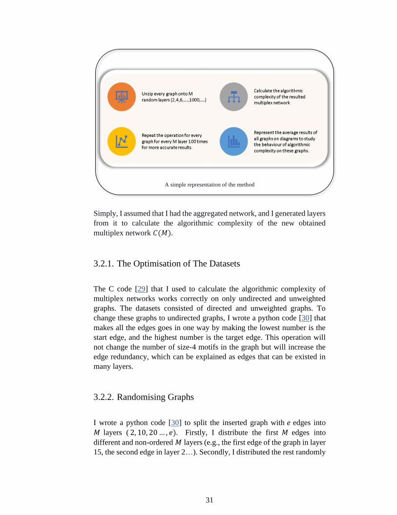
A simple representation of the method

Simply, I assumed that I had the aggregated network, and I generated layers

from it to calculate the algorithmic complexity of the new obtained

multiplex network 𝐶(𝑀).

3.2.1. The Optimisation of The Datasets

The C code [29] that I used to calculate the algorithmic complexity of

multiplex networks works correctly on only undirected and unweighted

graphs. The datasets consisted of directed and unweighted graphs. To

change these graphs to undirected graphs, I wrote a python code [30] that

makes all the edges goes in one way by making the lowest number is the

start edge, and the highest number is the target edge. This operation will

not change the number of size-4 motifs in the graph but will increase the

edge redundancy, which can be explained as edges that can be existed in

many layers.

3.2.2. Randomising Graphs

I wrote a python code [30] to split the inserted graph with 𝑒 edges into

𝑀 layers ( 2, 10, 20 … , 𝑒). Firstly, I distribute the first 𝑀 edges into

different and non-ordered 𝑀 layers (e.g., the first edge of the graph in layer

15, the second edge in layer 2…). Secondly, I distributed the rest randomly

32

(𝑒 − 𝑀) among these constructed 𝑀 layers. I did this operation on every

graph 100 times for every 𝑀.

3.2.3. Calculating Algorithmic Complexity of Graphs

The used method to measure the algorithmic complexity is from A Santoro

and V Nicosia GitHub page [29]. For running the C code, it needs the

following:

• A text file containing the edge list of each layer of the multiplex.

• A text file containing the list of layers.

• A text file containing the list of unique IDs appearing within the

multiplex network.

Check the folder example on the GitHub page [29] for more details. The

datasets consist of single layer graphs. I wrote a python code to create all

the requested files for each case of graph randomisation on 𝑀 layers.

33

Chapter 4

4. Results

I had two main sets of graphs. The first set consists of 11 subsets of graphs

with 100 nodes, 986 edges and the number of motifs of size-4 is between

50 000 – 300 000. The first set consists of 5 subsets of graphs with 200

nodes, 3800 edges and the number of motifs of size-4 is between 3 000 000

– 3 400 000. I chose to display one detailed measurements of each main set

because there are too many diagrams. To see all detailed results, see

appendix B.

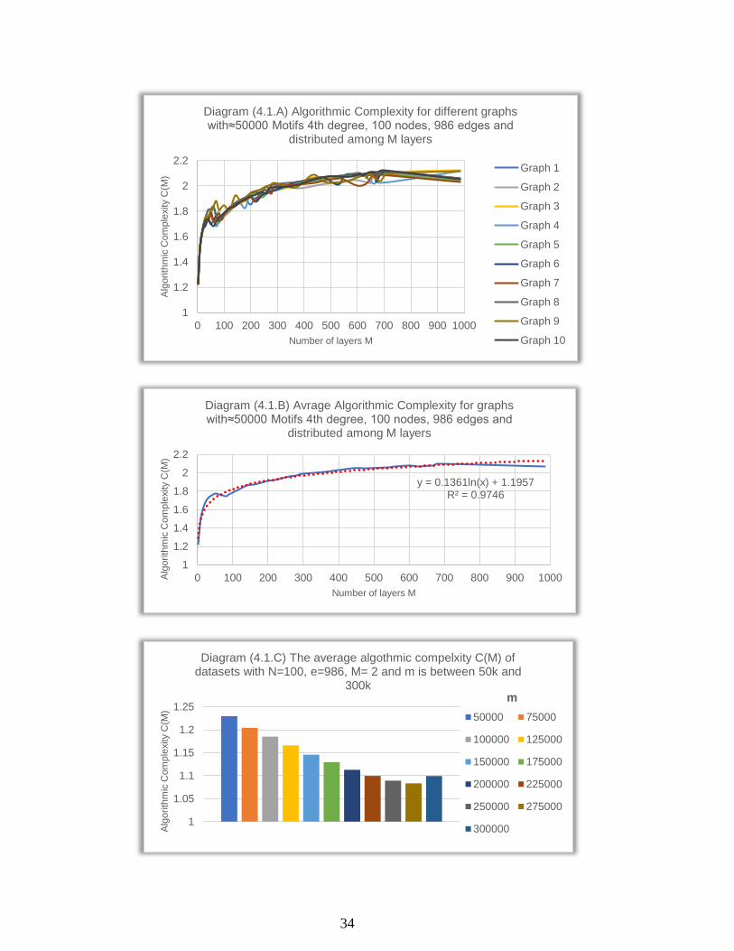
4.1. 1st dataset 𝑁=100, e ≈ 1000

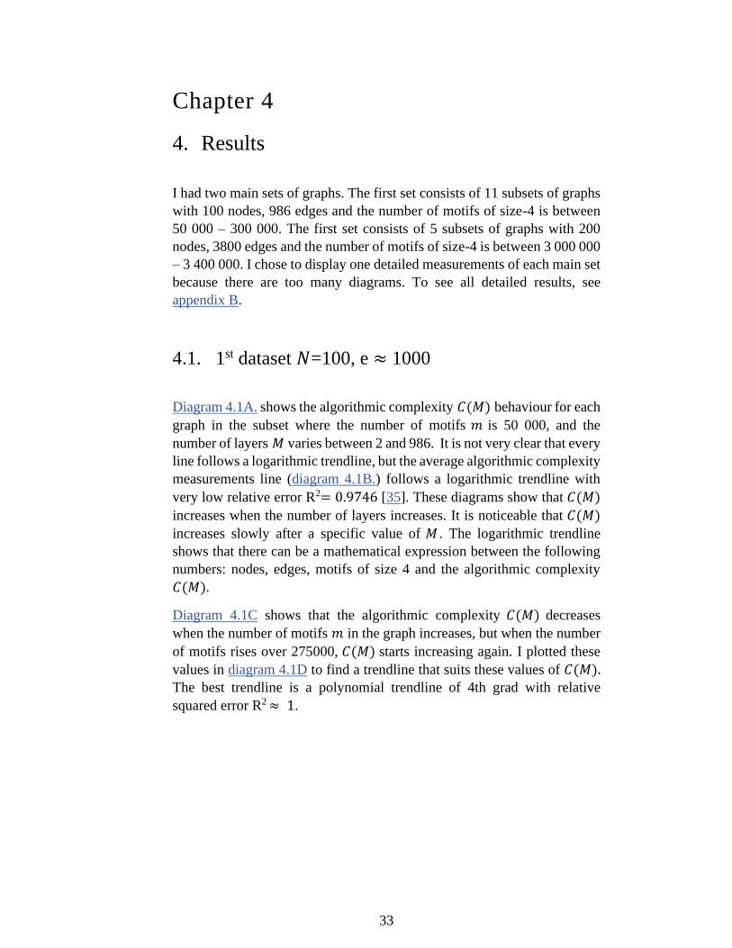
Diagram 4.1A. shows the algorithmic complexity 𝐶(𝑀) behaviour for each

graph in the subset where the number of motifs 𝑚 is 50 000, and the

number of layers 𝑀 varies between 2 and 986. It is not very clear that every

line follows a logarithmic trendline, but the average algorithmic complexity

measurements line (diagram 4.1B.) follows a logarithmic trendline with

very low relative error R2= 0.9746 [35]. These diagrams show that 𝐶(𝑀)

increases when the number of layers increases. It is noticeable that 𝐶(𝑀)

increases slowly after a specific value of 𝑀 . The logarithmic trendline

shows that there can be a mathematical expression between the following

numbers: nodes, edges, motifs of size 4 and the algorithmic complexity

𝐶(𝑀).

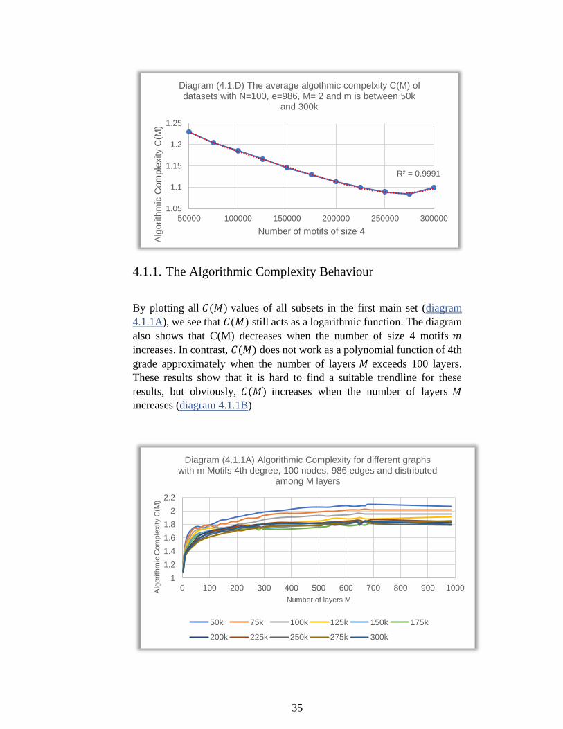
Diagram 4.1C shows that the algorithmic complexity 𝐶(𝑀) decreases

when the number of motifs 𝑚 in the graph increases, but when the number

of motifs rises over 275000, 𝐶(𝑀) starts increasing again. I plotted these

values in diagram 4.1D to find a trendline that suits these values of 𝐶(𝑀). The best trendline is a polynomial trendline of 4th grad with relative

squared error R2 ≈ 1.

34

1

1.2

1.4

1.6

1.8

2

2.2

0 100 200 300 400 500 600 700 800 900 1000

Alg

orith

mic

Com

ple

xity C

(M)

Number of layers M

Diagram (4.1.A) Algorithmic Complexity for different graphs with≈50000 Motifs 4th degree, 100 nodes, 986 edges and

distributed among M layers

Graph 1

Graph 2

Graph 3

Graph 4

Graph 5

Graph 6

Graph 7

Graph 8

Graph 9

Graph 10

y = 0.1361ln(x) + 1.1957R² = 0.9746

1

1.2

1.4

1.6

1.8

2

2.2

0 100 200 300 400 500 600 700 800 900 1000Alg

orith

mic

Com

ple

xity C

(M)

Number of layers M

Diagram (4.1.B) Avrage Algorithmic Complexity for graphs with≈50000 Motifs 4th degree, 100 nodes, 986 edges and

distributed among M layers

1

1.05

1.1

1.15

1.2

1.25

Alg

orith

mic

Com

ple

xity C

(M)

m

Diagram (4.1.C) The average algothmic compelxity C(M) of datasets with N=100, e=986, M= 2 and m is between 50k and

300k

50000 75000

100000 125000

150000 175000

200000 225000

250000 275000

300000

35

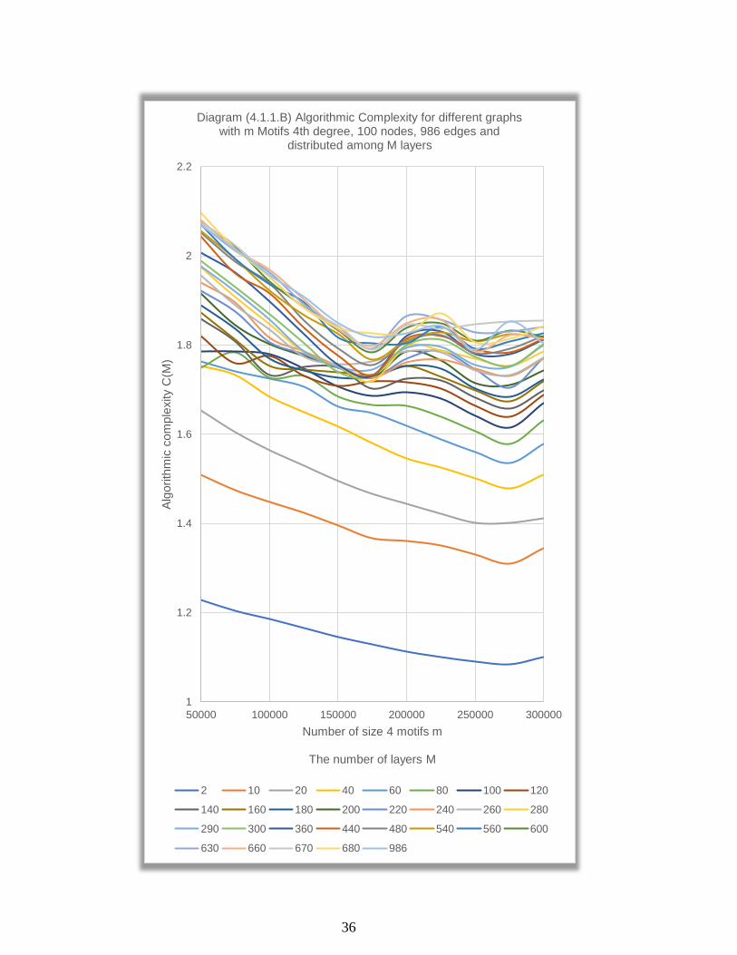
4.1.1. The Algorithmic Complexity Behaviour

By plotting all 𝐶(𝑀) values of all subsets in the first main set (diagram

4.1.1A), we see that 𝐶(𝑀) still acts as a logarithmic function. The diagram

also shows that C(M) decreases when the number of size 4 motifs 𝑚

increases. In contrast, 𝐶(𝑀) does not work as a polynomial function of 4th

grade approximately when the number of layers 𝑀 exceeds 100 layers.

These results show that it is hard to find a suitable trendline for these

results, but obviously, 𝐶(𝑀) increases when the number of layers 𝑀

increases (diagram 4.1.1B).

R² = 0.9991

1.05

1.1

1.15

1.2

1.25

50000 100000 150000 200000 250000 300000

Alg

orith

mic

Com

ple

xity

C(M

)

Number of motifs of size 4

Diagram (4.1.D) The average algothmic compelxity C(M) of datasets with N=100, e=986, M= 2 and m is between 50k

and 300k

1

1.2

1.4

1.6

1.8

2

2.2

0 100 200 300 400 500 600 700 800 900 1000Alg

orith

mic

Com

ple

xity C

(M)

Number of layers M

Diagram (4.1.1A) Algorithmic Complexity for different graphs with m Motifs 4th degree, 100 nodes, 986 edges and distributed

among M layers

50k 75k 100k 125k 150k 175k

200k 225k 250k 275k 300k

36

1

1.2

1.4

1.6

1.8

2

2.2

50000 100000 150000 200000 250000 300000

Alg

orith

mic

com

ple

xity C

(M)

Number of size 4 motifs m

The number of layers M

Diagram (4.1.1.B) Algorithmic Complexity for different graphs with m Motifs 4th degree, 100 nodes, 986 edges and

distributed among M layers

2 10 20 40 60 80 100 120

140 160 180 200 220 240 260 280

290 300 360 440 480 540 560 600

630 660 670 680 986

37

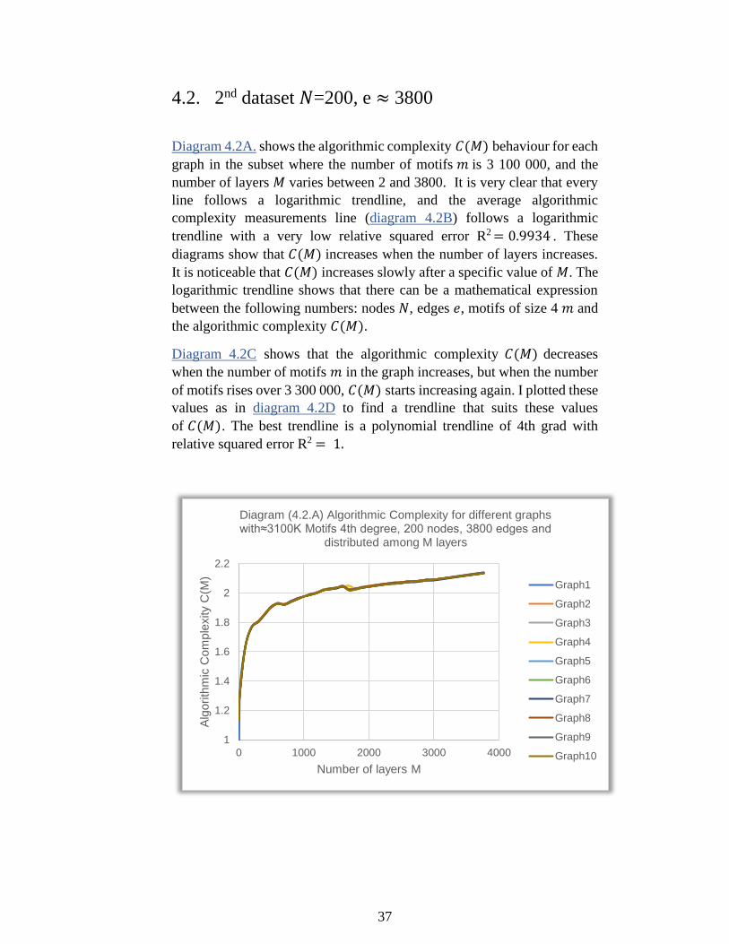
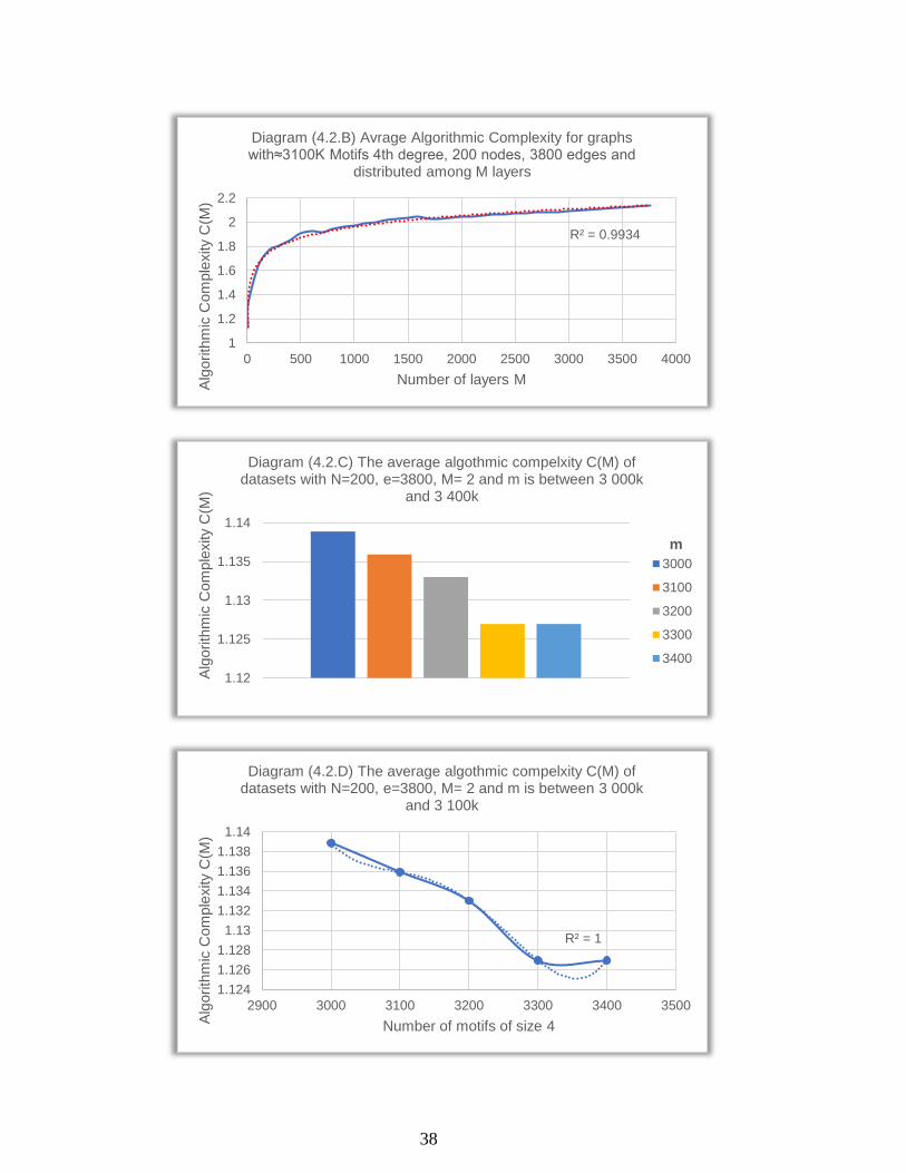
4.2. 2nd dataset 𝑁=200, e ≈ 3800

Diagram 4.2A. shows the algorithmic complexity 𝐶(𝑀) behaviour for each

graph in the subset where the number of motifs 𝑚 is 3 100 000, and the

number of layers 𝑀 varies between 2 and 3800. It is very clear that every

line follows a logarithmic trendline, and the average algorithmic

complexity measurements line (diagram 4.2B) follows a logarithmic

trendline with a very low relative squared error R2 = 0.9934 . These

diagrams show that 𝐶(𝑀) increases when the number of layers increases.

It is noticeable that 𝐶(𝑀) increases slowly after a specific value of 𝑀. The

logarithmic trendline shows that there can be a mathematical expression

between the following numbers: nodes 𝑁, edges 𝑒, motifs of size 4 𝑚 and

the algorithmic complexity 𝐶(𝑀).

Diagram 4.2C shows that the algorithmic complexity 𝐶(𝑀) decreases

when the number of motifs 𝑚 in the graph increases, but when the number

of motifs rises over 3 300 000, 𝐶(𝑀) starts increasing again. I plotted these

values as in diagram 4.2D to find a trendline that suits these values

of 𝐶(𝑀). The best trendline is a polynomial trendline of 4th grad with

relative squared error R2 = 1.

1

1.2

1.4

1.6

1.8

2

2.2

0 1000 2000 3000 4000

Alg

orith

mic

Com

ple

xity C

(M)

Number of layers M

Diagram (4.2.A) Algorithmic Complexity for different graphs with≈3100K Motifs 4th degree, 200 nodes, 3800 edges and

distributed among M layers

Graph1

Graph2

Graph3

Graph4

Graph5

Graph6

Graph7

Graph8

Graph9

Graph10

38

R² = 0.9934

1

1.2

1.4

1.6

1.8

2

2.2

0 500 1000 1500 2000 2500 3000 3500 4000

Alg

orith

mic

Com

ple

xity

C(M

)

Number of layers M

Diagram (4.2.B) Avrage Algorithmic Complexity for graphs with≈3100K Motifs 4th degree, 200 nodes, 3800 edges and

distributed among M layers

1.12

1.125

1.13

1.135

1.14

Alg

orith

mic

Com

ple

xity C

(M)

m

Diagram (4.2.C) The average algothmic compelxity C(M) of datasets with N=200, e=3800, M= 2 and m is between 3 000k

and 3 400k

3000

3100

3200

3300

3400

R² = 1

1.124

1.126

1.128

1.13

1.132

1.134

1.136

1.138

1.14

2900 3000 3100 3200 3300 3400 3500

Alg

orith

mic

Com

ple

xity

C(M

)

Number of motifs of size 4

Diagram (4.2.D) The average algothmic compelxity C(M) of datasets with N=200, e=3800, M= 2 and m is between 3 000k

and 3 100k

39

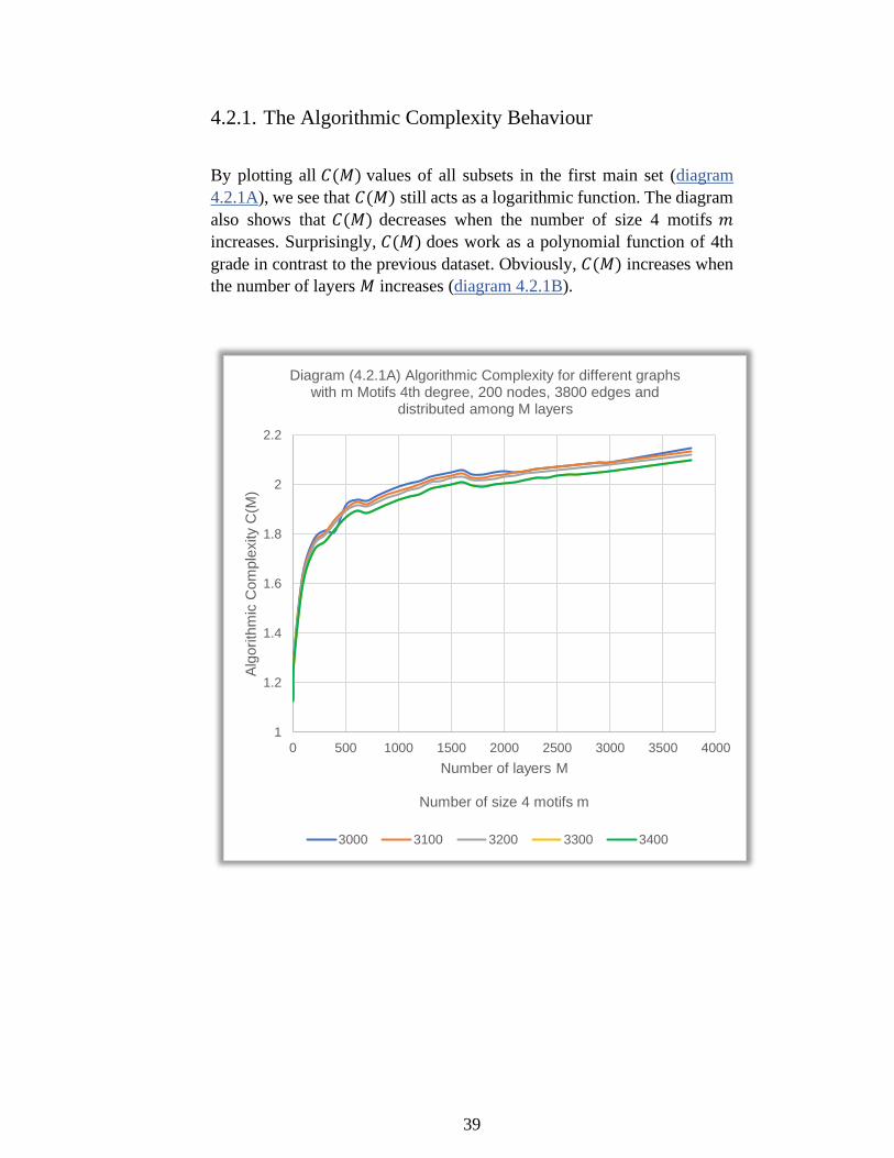
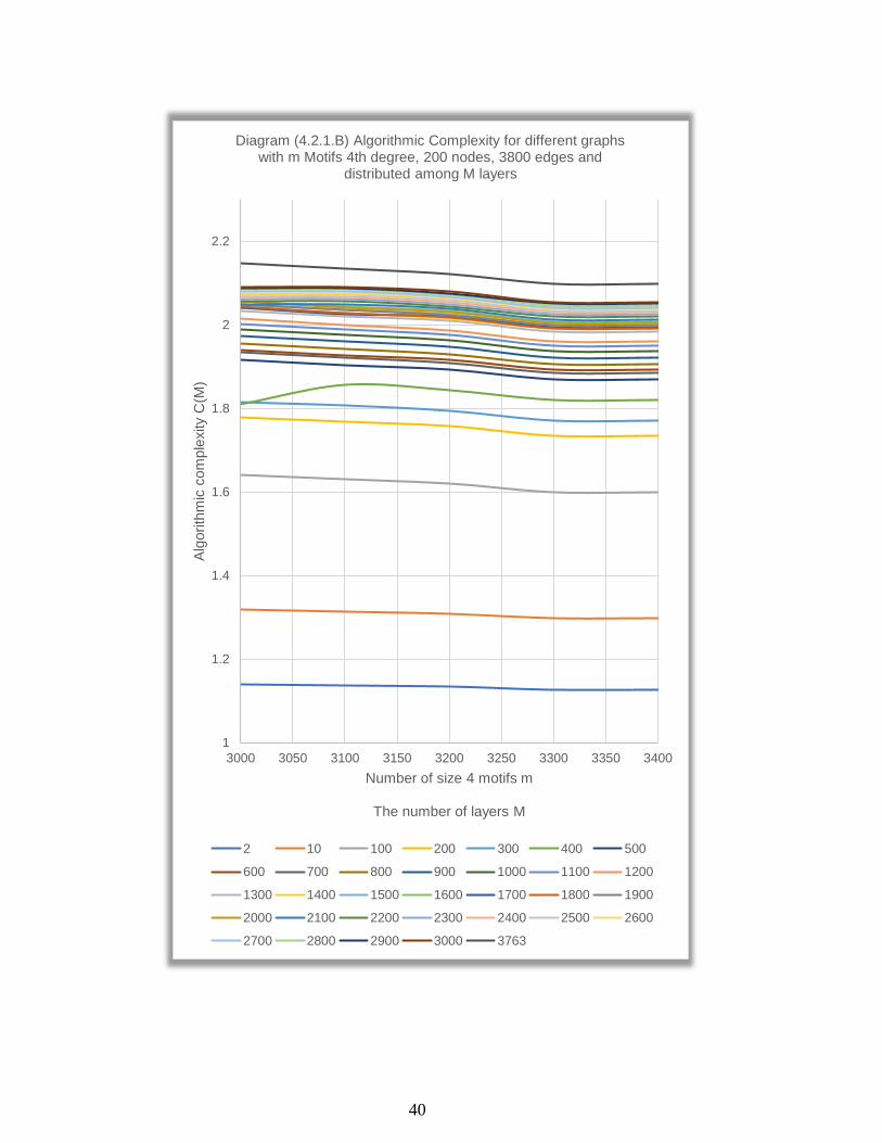
4.2.1. The Algorithmic Complexity Behaviour

By plotting all 𝐶(𝑀) values of all subsets in the first main set (diagram

4.2.1A), we see that 𝐶(𝑀) still acts as a logarithmic function. The diagram

also shows that 𝐶(𝑀) decreases when the number of size 4 motifs 𝑚

increases. Surprisingly, 𝐶(𝑀) does work as a polynomial function of 4th

grade in contrast to the previous dataset. Obviously, 𝐶(𝑀) increases when

the number of layers 𝑀 increases (diagram 4.2.1B).

1

1.2

1.4

1.6

1.8

2

2.2

0 500 1000 1500 2000 2500 3000 3500 4000

Alg

orith

mic

Com

ple

xity C

(M)

Number of layers M

Number of size 4 motifs m

Diagram (4.2.1A) Algorithmic Complexity for different graphs with m Motifs 4th degree, 200 nodes, 3800 edges and

distributed among M layers

3000 3100 3200 3300 3400

40

1

1.2

1.4

1.6

1.8

2

2.2

3000 3050 3100 3150 3200 3250 3300 3350 3400

Alg

orith

mic

com

ple

xity C

(M)

Number of size 4 motifs m

The number of layers M

Diagram (4.2.1.B) Algorithmic Complexity for different graphs with m Motifs 4th degree, 200 nodes, 3800 edges and

distributed among M layers

2 10 100 200 300 400 500

600 700 800 900 1000 1100 1200

1300 1400 1500 1600 1700 1800 1900

2000 2100 2200 2300 2400 2500 2600

2700 2800 2900 3000 3763

41

Chapter 5

5. Discussion

We live in a continuous expansion of networks these days and more

discoveries and strategies that link different complex systems (e.g.,

correlating cycle-road map with public transport map in Google maps to

give us the best way to reach our destination.). Quantifying the structural

information encoded in a network has fundamental importance to identify

the components of the system it represents. Talking about the complex

systems, assessing the actual amount of information contributed by each

additional layer attracts more attention from scientists. Regarding the latest

trends in data science, more data is not always good because it can cause

more unnecessary redundant information that means more noise.

Comparing different graphs regarding their complexity is vital because it

has many benefits, such as giving initial thoughts about the graph or system

we are dealing with by comparing it with other graphs or systems [1].

Consequently, ranking different multiplex networks according to their

value of 𝐶(𝑀) is meaningful. Since those values are indeed telling us how

much a multiplex representation deviates from the corresponding null-

model hypothesis, i.e., that the system can be represented instead as a

single-layer graph.

5.1. The quality of 𝐶(𝑀)

The algorithmic information approach proposed in this paper condenses the

structural properties of a multiplex in a number—the multiplex

complexity 𝐶(𝑀) which is defined as the ratio between the Kolmogorov

complexity of the multiplex network and that of the corresponding

aggregated graph. Its values allow us to assess to which extent a given

multiplex representation of a system is more informative than a single-layer

graph (e.g., if 𝐶(𝑀)is higher than 1). The multiplex complexity 𝐶(𝑀)

proposed here links quite closely to the traditional meaning of complexity

of a system as the amount of information needed to describe it

meaningfully. This link is made possible by the prime-weight matrix,

which encodes the comprehensive structure of the system in a string of bits.

It is true that, in principle, the prime-weight matrix encoding depends on

the chosen assignment of labels to nodes and primes to layers. This

42

representation does not lose any information about the original system, and

it is perfectly lossless. The prime-weight matrix preserves information

about the multiplex network 𝑀, i.e., about the placement of all its edges.

We do that to make it always possible to get back to the original graph by

factoring in the prime numbers we have written down [31]. Remarkably,

the assignment of primes to layers in increasing order of the total number

of edges provides a consistent approximation of Kolmogorov complexity,

although a conservative one. Because of the way 𝐶(𝑀) is defined, its value

varies in a somehow predictable way if the edges of the graph are

reorganized. If we add an edge to an existing multiplex, then we can expect

the value of multiplex complexity to change only slightly. In this sense,

𝐶(𝑀) is more closely associated with the system structure, and its changes

provide information that is more readily interpretable [1].

If we change the compression algorithm, the results will change, and we

cannot also tell how good the bound we get is. But if we use the same

algorithm (Gzip in this case) on different systems, we still can compare the

relative complexity of various systems robustly.

5.2. The quality of heuristics and heuristic results

By looking to the relative squared error in the measurements, we can see

that the results are reliable and have high quality. Randomising the graphs

more than 100 times will give us more accurate results because more

attempts lead to better results. Because randomising a graph and calculating

its algorithmic complexity 𝐶(𝑀) takes long time, I was not able to do the

operation more 100 times regarding the time and the processing speed I

had. The results could be even more accurate if I had a more comprehensive

dataset, e.g., more than ten graphs with the same properties and more sets

with lower/higher amount motifs.

43

Chapter 6

6. Conclusion

Surprisingly, the results show that algorithmic complexity 𝐶(𝑀) has the

same logarithmic mathematical behaviour on different graphs. The most

interesting conclusion is that 𝐶(𝑀) can be expressed in logarithmic

mathematical expression with the following terms: the number of nodes 𝑁,

the number of motifs 𝑚, the number of edges 𝑒, and the number of layers

𝑀 . Forming this expression will move this problem will move graph

complexity problem out of the NP-hard range. It will also allow us to

estimate the number of motifs m or the complexity without using

complicated algorithms and programs. We can define the complexity of a

graph with the following statement: the complexity of a graph (that has 𝑒

edges) is the algorithmic complexity of multiplex networks 𝐶(𝑀) of that

graph distributed among 𝑀 = 𝑒 layers (i.e., 𝐶(𝑒)). This definition will

allow the comparison of graphs regarding their complexity.

Further research

To concrete the results and find the mathematical expression of the

complexity of graphs the following research is needed:

• Test the heuristics of complexity on other types of graphs to

confirm the results. I.e., different number of edges 𝑒, different

number of nodes 𝑁, different motif size and wider range of the

number of motifs 𝑚.

• Mathematical research is needed to find the logarithmic equation

of graph complexity in terms of 𝑁, 𝑒, 𝑚, and 𝑀.

44

Chapter 7

7. Appendices

Appendix A

Prime-Weight Matrix Encoding

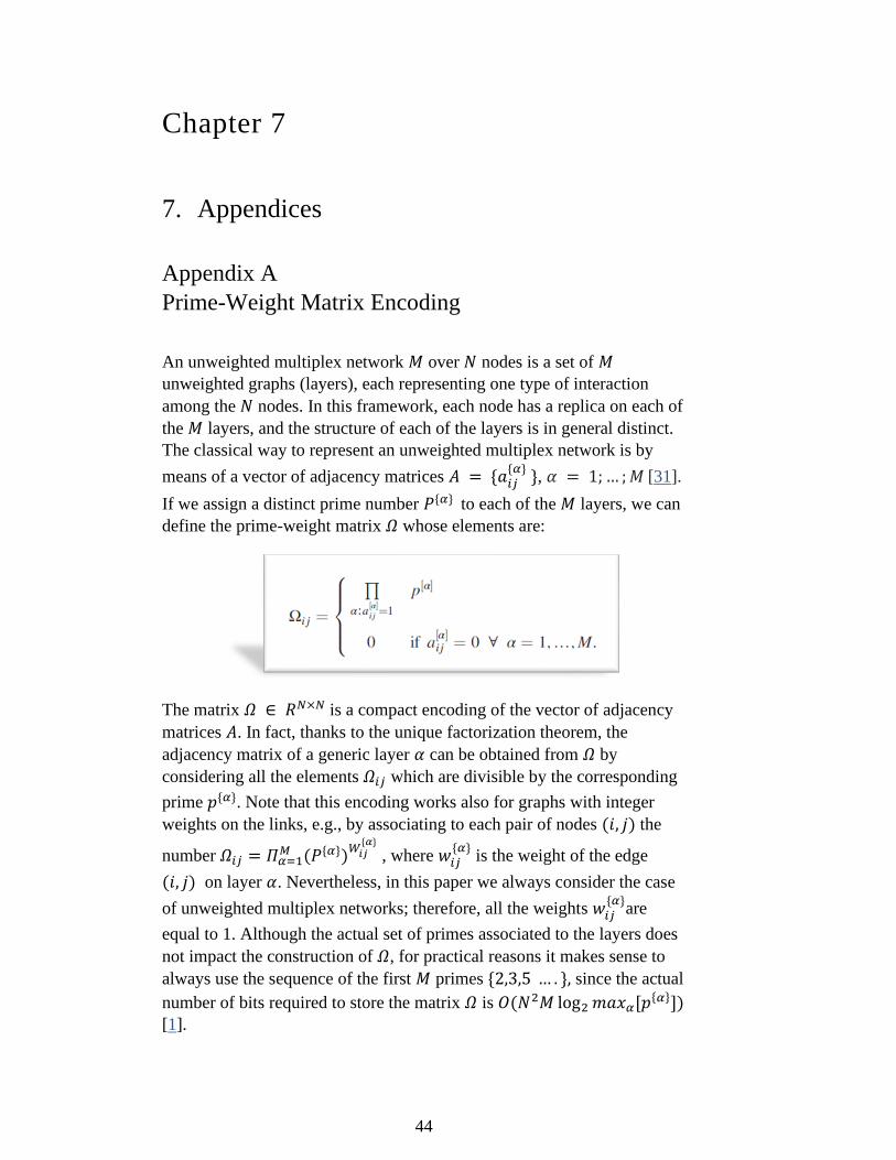
An unweighted multiplex network 𝑀 over 𝑁 nodes is a set of 𝑀

unweighted graphs (layers), each representing one type of interaction

among the 𝑁 nodes. In this framework, each node has a replica on each of

the 𝑀 layers, and the structure of each of the layers is in general distinct.

The classical way to represent an unweighted multiplex network is by

means of a vector of adjacency matrices 𝐴 = {𝑎𝑖𝑗{𝛼}

}, 𝛼 = 1; … ; 𝑀 [31].

If we assign a distinct prime number 𝑃{𝛼} to each of the 𝑀 layers, we can

define the prime-weight matrix 𝛺 whose elements are:

The matrix 𝛺 ∈ 𝑅𝑁×𝑁 is a compact encoding of the vector of adjacency

matrices 𝐴. In fact, thanks to the unique factorization theorem, the

adjacency matrix of a generic layer 𝛼 can be obtained from 𝛺 by

considering all the elements 𝛺𝑖𝑗 which are divisible by the corresponding

prime 𝑝{𝛼}. Note that this encoding works also for graphs with integer

weights on the links, e.g., by associating to each pair of nodes (𝑖, 𝑗) the

number 𝛺𝑖𝑗 = 𝛱𝛼=1𝑀 (𝑃{𝛼})

𝑊𝑖𝑗{𝛼}

, where 𝑤𝑖𝑗{𝛼}

is the weight of the edge

(𝑖, 𝑗) on layer 𝛼. Nevertheless, in this paper we always consider the case

of unweighted multiplex networks; therefore, all the weights 𝑤𝑖𝑗{𝛼}

are

equal to 1. Although the actual set of primes associated to the layers does

not impact the construction of 𝛺, for practical reasons it makes sense to

always use the sequence of the first 𝑀 primes {2,3,5 … . }, since the actual

number of bits required to store the matrix 𝛺 is 𝑂(𝑁2𝑀 log2 𝑚𝑎𝑥𝛼[𝑝{𝛼}])

[1].

45

Appendix B

Detailed Results

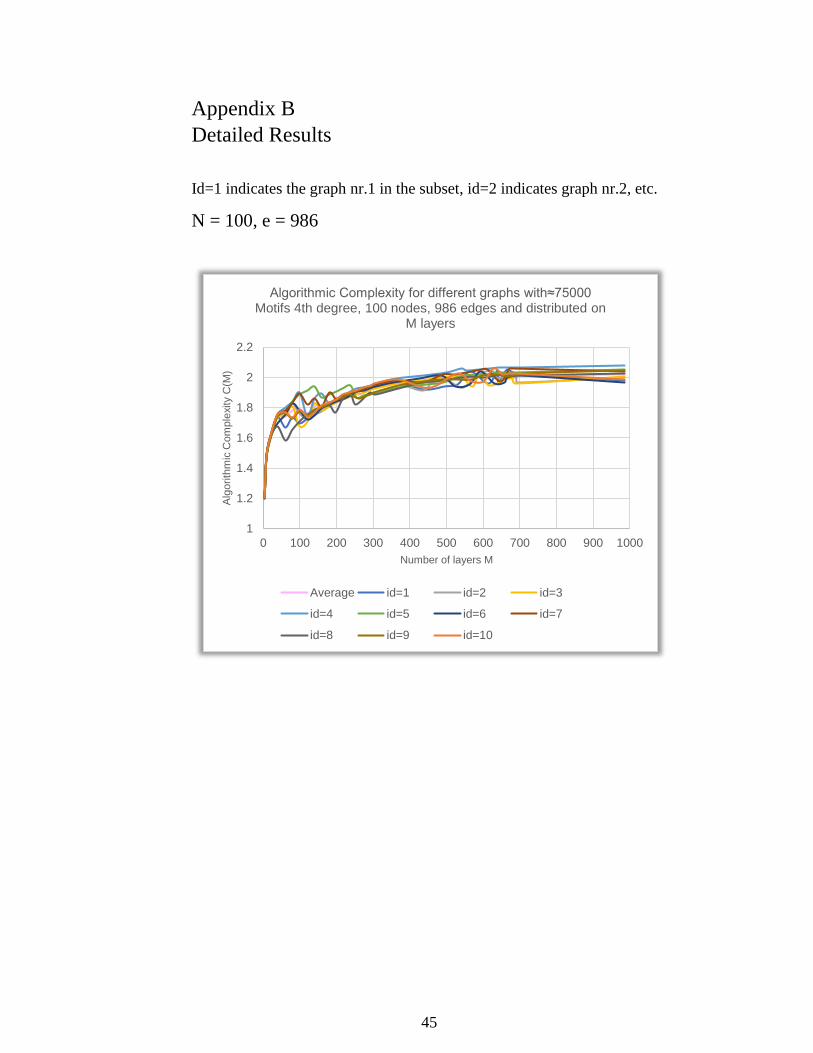
Id=1 indicates the graph nr.1 in the subset, id=2 indicates graph nr.2, etc.

N = 100, e = 986

1

1.2

1.4

1.6

1.8

2

2.2

0 100 200 300 400 500 600 700 800 900 1000

Alg

orith

mic

Com

ple

xity C

(M)

Number of layers M

Algorithmic Complexity for different graphs with≈75000 Motifs 4th degree, 100 nodes, 986 edges and distributed on

M layers

Average id=1 id=2 id=3

id=4 id=5 id=6 id=7

id=8 id=9 id=10

46

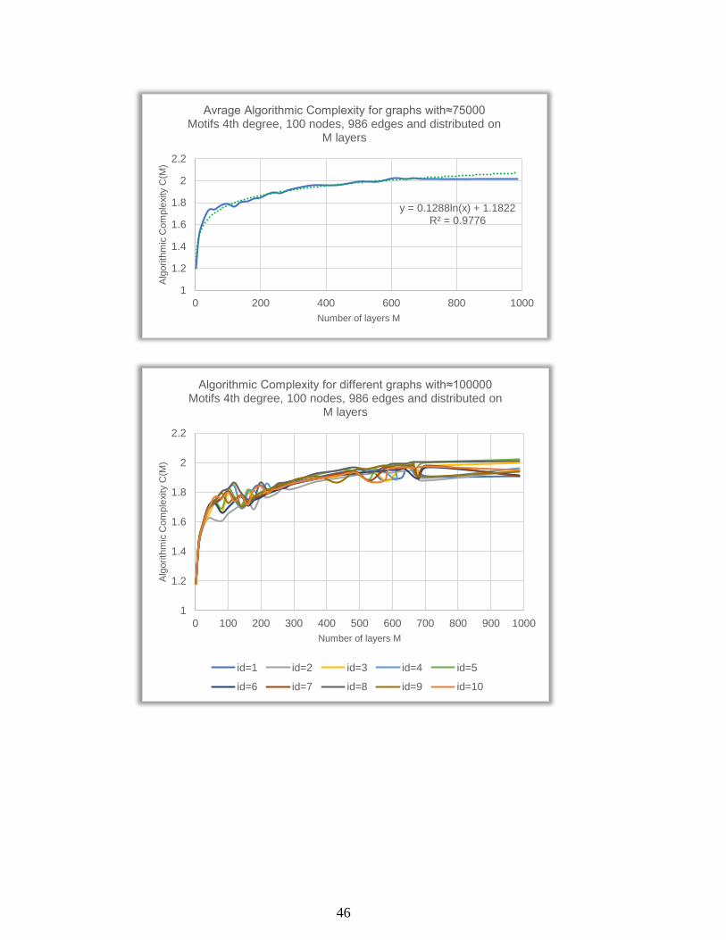
y = 0.1288ln(x) + 1.1822R² = 0.9776

1

1.2

1.4

1.6

1.8

2

2.2

0 200 400 600 800 1000

Alg

orith

mic

Com

ple

xity C

(M)

Number of layers M

Avrage Algorithmic Complexity for graphs with≈75000 Motifs 4th degree, 100 nodes, 986 edges and distributed on

M layers

1

1.2

1.4

1.6

1.8

2

2.2

0 100 200 300 400 500 600 700 800 900 1000

Alg

orith

mic

Com

ple

xity C

(M)

Number of layers M

Algorithmic Complexity for different graphs with≈100000 Motifs 4th degree, 100 nodes, 986 edges and distributed on

M layers

id=1 id=2 id=3 id=4 id=5

id=6 id=7 id=8 id=9 id=10

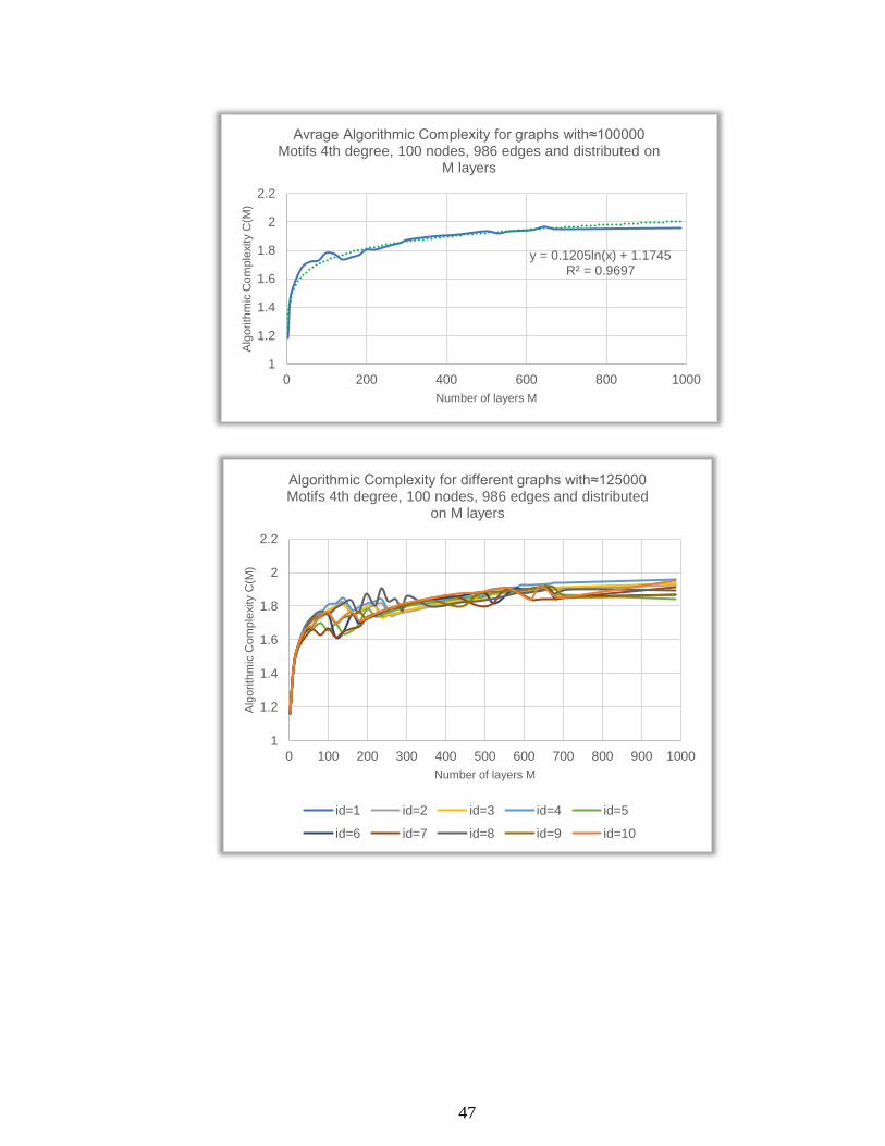
47

y = 0.1205ln(x) + 1.1745R² = 0.9697

1

1.2

1.4

1.6

1.8

2

2.2

0 200 400 600 800 1000

Alg

orith

mic

Com

ple

xity C

(M)

Number of layers M

Avrage Algorithmic Complexity for graphs with≈100000 Motifs 4th degree, 100 nodes, 986 edges and distributed on

M layers

1

1.2

1.4

1.6

1.8

2

2.2

0 100 200 300 400 500 600 700 800 900 1000

Alg

orith

mic

Com

ple

xity C

(M)

Number of layers M

Algorithmic Complexity for different graphs with≈125000 Motifs 4th degree, 100 nodes, 986 edges and distributed

on M layers

id=1 id=2 id=3 id=4 id=5

id=6 id=7 id=8 id=9 id=10

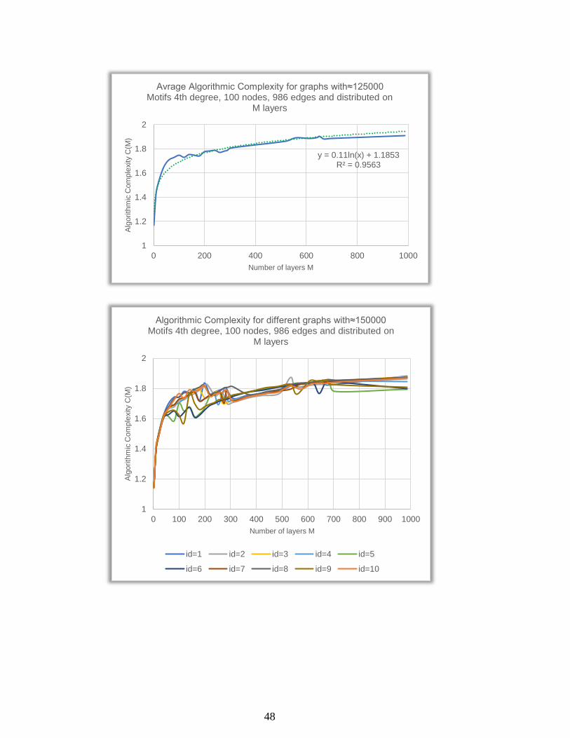
48

y = 0.11ln(x) + 1.1853R² = 0.9563

1

1.2

1.4

1.6

1.8

2

0 200 400 600 800 1000

Alg

orith

mic

Com

ple

xity C

(M)

Number of layers M

Avrage Algorithmic Complexity for graphs with≈125000 Motifs 4th degree, 100 nodes, 986 edges and distributed on

M layers

1

1.2

1.4

1.6

1.8

2

0 100 200 300 400 500 600 700 800 900 1000

Alg

orith

mic

Com

ple

xity C

(M)

Number of layers M

Algorithmic Complexity for different graphs with≈150000 Motifs 4th degree, 100 nodes, 986 edges and distributed on

M layers

id=1 id=2 id=3 id=4 id=5

id=6 id=7 id=8 id=9 id=10

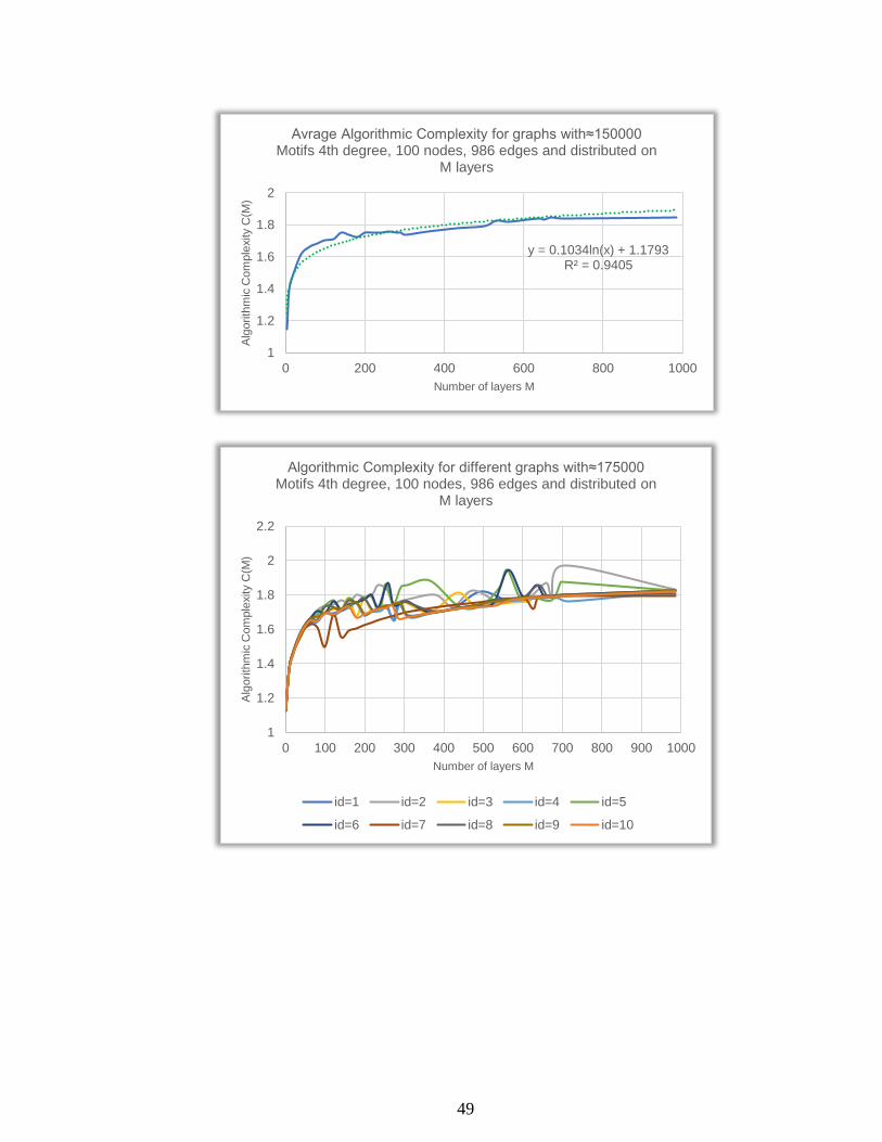
49

y = 0.1034ln(x) + 1.1793R² = 0.9405

1

1.2

1.4

1.6

1.8

2

0 200 400 600 800 1000

Alg

orith

mic

Com

ple

xity C

(M)

Number of layers M

Avrage Algorithmic Complexity for graphs with≈150000 Motifs 4th degree, 100 nodes, 986 edges and distributed on

M layers

1

1.2

1.4

1.6

1.8

2

2.2

0 100 200 300 400 500 600 700 800 900 1000

Alg

orith

mic

Com

ple

xity C

(M)

Number of layers M

Algorithmic Complexity for different graphs with≈175000 Motifs 4th degree, 100 nodes, 986 edges and distributed on

M layers

id=1 id=2 id=3 id=4 id=5

id=6 id=7 id=8 id=9 id=10

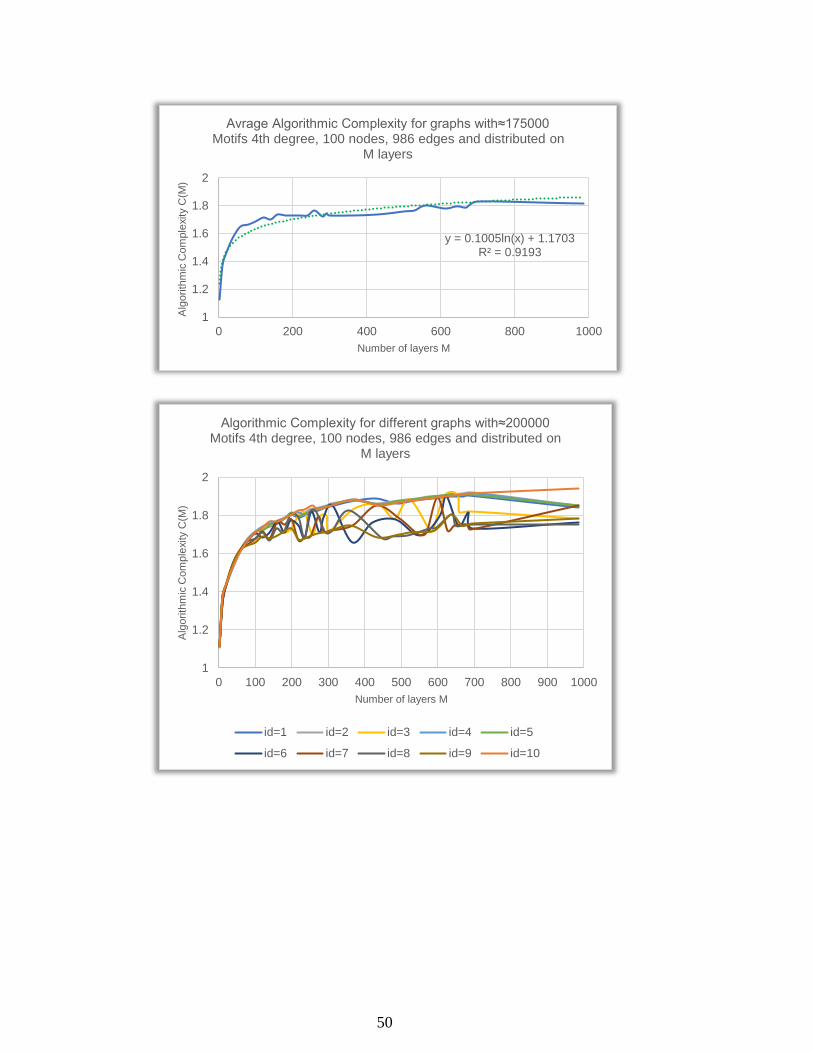
50

y = 0.1005ln(x) + 1.1703R² = 0.9193

1

1.2

1.4

1.6

1.8

2

0 200 400 600 800 1000

Alg

orith

mic

Com

ple

xity C

(M)

Number of layers M

Avrage Algorithmic Complexity for graphs with≈175000 Motifs 4th degree, 100 nodes, 986 edges and distributed on

M layers

1

1.2

1.4

1.6

1.8

2

0 100 200 300 400 500 600 700 800 900 1000

Alg

orith

mic

Com

ple

xity C

(M)

Number of layers M

Algorithmic Complexity for different graphs with≈200000 Motifs 4th degree, 100 nodes, 986 edges and distributed on

M layers

id=1 id=2 id=3 id=4 id=5

id=6 id=7 id=8 id=9 id=10

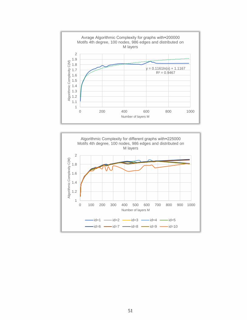
51

y = 0.1161ln(x) + 1.1167R² = 0.9467

1

1.1

1.2

1.3

1.4

1.5

1.6

1.7

1.8

1.9

2

0 200 400 600 800 1000

Alg

orith

mic

Com

ple

xity C

(M)

Number of layers M

Avrage Algorithmic Complexity for graphs with≈200000 Motifs 4th degree, 100 nodes, 986 edges and distributed on

M layers

1

1.2

1.4

1.6

1.8

2

0 100 200 300 400 500 600 700 800 900 1000

Alg

orith

mic

Com

ple

xity C

(M)

Number of layers M

Algorithmic Complexity for different graphs with≈225000 Motifs 4th degree, 100 nodes, 986 edges and distributed on

M layers

id=1 id=2 id=3 id=4 id=5

id=6 id=7 id=8 id=9 id=10

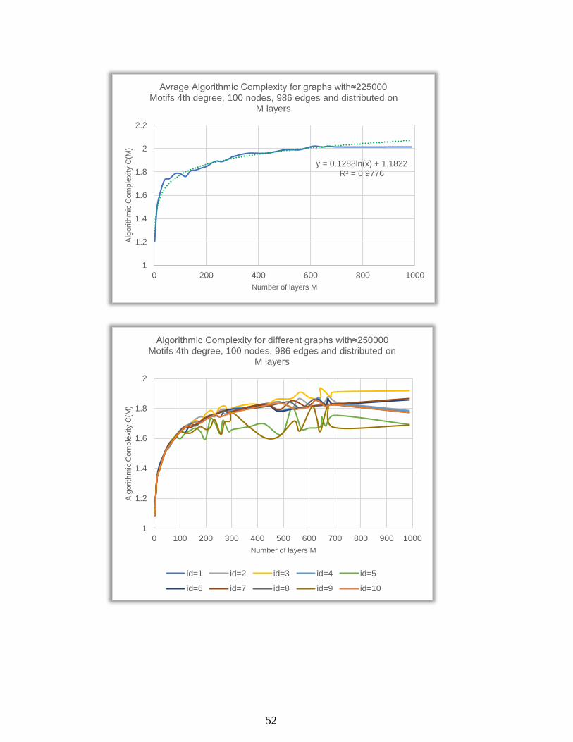
52

y = 0.1288ln(x) + 1.1822R² = 0.9776

1

1.2

1.4

1.6

1.8

2

2.2

0 200 400 600 800 1000

Alg

orith

mic

Com

ple

xity C

(M)

Number of layers M

Avrage Algorithmic Complexity for graphs with≈225000 Motifs 4th degree, 100 nodes, 986 edges and distributed on

M layers

1

1.2

1.4

1.6

1.8

2

0 100 200 300 400 500 600 700 800 900 1000

Alg

orith

mic

Com

ple

xity C

(M)

Number of layers M

Algorithmic Complexity for different graphs with≈250000 Motifs 4th degree, 100 nodes, 986 edges and distributed on

M layers

id=1 id=2 id=3 id=4 id=5

id=6 id=7 id=8 id=9 id=10

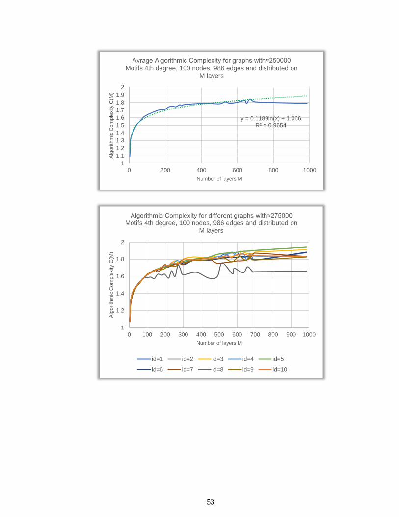
53

y = 0.1189ln(x) + 1.066R² = 0.9654

1

1.1

1.2

1.3

1.4

1.5

1.6

1.7

1.8

1.9

2

0 200 400 600 800 1000

Alg

orith

mic

Com

ple

xity C

(M)

Number of layers M

Avrage Algorithmic Complexity for graphs with≈250000 Motifs 4th degree, 100 nodes, 986 edges and distributed on

M layers

1

1.2

1.4

1.6

1.8

2

0 100 200 300 400 500 600 700 800 900 1000

Alg

orith

mic

Com

ple

xity C

(M)

Number of layers M

Algorithmic Complexity for different graphs with≈275000 Motifs 4th degree, 100 nodes, 986 edges and distributed on

M layers

id=1 id=2 id=3 id=4 id=5

id=6 id=7 id=8 id=9 id=10

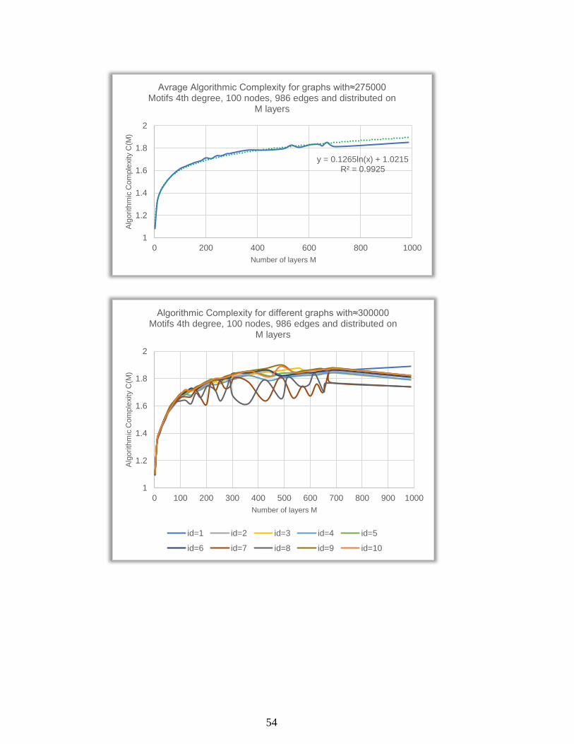
54

y = 0.1265ln(x) + 1.0215R² = 0.9925

1

1.2

1.4

1.6

1.8

2

0 200 400 600 800 1000

Alg

orith

mic

Com

ple

xity C

(M)

Number of layers M

Avrage Algorithmic Complexity for graphs with≈275000 Motifs 4th degree, 100 nodes, 986 edges and distributed on

M layers

1

1.2

1.4

1.6

1.8

2

0 100 200 300 400 500 600 700 800 900 1000

Alg

orith

mic

Com

ple

xity C

(M)

Number of layers M

Algorithmic Complexity for different graphs with≈300000 Motifs 4th degree, 100 nodes, 986 edges and distributed on

M layers

id=1 id=2 id=3 id=4 id=5

id=6 id=7 id=8 id=9 id=10

55

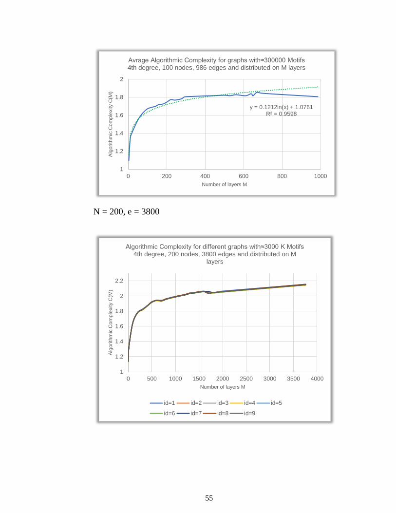
N = 200, e = 3800

y = 0.1212ln(x) + 1.0761R² = 0.9598

1

1.2

1.4

1.6

1.8

2

0 200 400 600 800 1000

Alg

orith

mic

Com

ple

xity C

(M)

Number of layers M

Avrage Algorithmic Complexity for graphs with≈300000 Motifs 4th degree, 100 nodes, 986 edges and distributed on M layers

1

1.2

1.4

1.6

1.8

2

2.2

0 500 1000 1500 2000 2500 3000 3500 4000

Alg

orith

mic

Com

ple

xity C

(M)

Number of layers M

Algorithmic Complexity for different graphs with≈3000 K Motifs 4th degree, 200 nodes, 3800 edges and distributed on M

layers

id=1 id=2 id=3 id=4 id=5

id=6 id=7 id=8 id=9

56

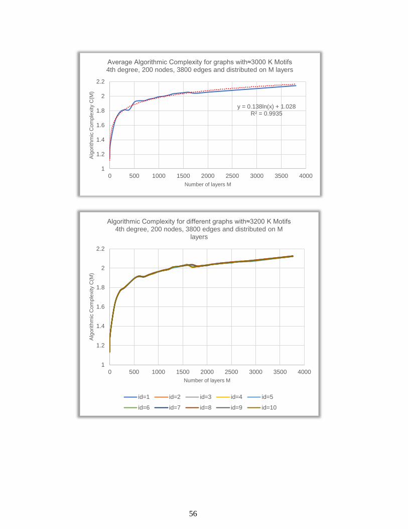
y = 0.138ln(x) + 1.028R² = 0.9935

1

1.2

1.4

1.6

1.8

2

2.2

0 500 1000 1500 2000 2500 3000 3500 4000

Alg

orith

mic

Com

ple

xity C

(M)

Number of layers M

Average Algorithmic Complexity for graphs with≈3000 K Motifs 4th degree, 200 nodes, 3800 edges and distributed on M layers

1

1.2

1.4

1.6

1.8

2

2.2

0 500 1000 1500 2000 2500 3000 3500 4000

Alg

orith

mic

Com

ple

xity C

(M)

Number of layers M

Algorithmic Complexity for different graphs with≈3200 K Motifs 4th degree, 200 nodes, 3800 edges and distributed on M

layers

id=1 id=2 id=3 id=4 id=5

id=6 id=7 id=8 id=9 id=10

57

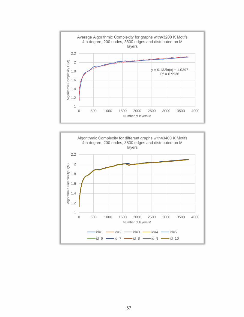
y = 0.132ln(x) + 1.0397R² = 0.9936

1

1.2

1.4

1.6

1.8

2

2.2

0 500 1000 1500 2000 2500 3000 3500 4000

Alg

orith

mic

Com

ple

xity C

(M)

Number of layers M

Average Algorithmic Complexity for graphs with≈3200 K Motifs 4th degree, 200 nodes, 3800 edges and distributed on M

layers

1

1.2

1.4

1.6

1.8

2

2.2

0 500 1000 1500 2000 2500 3000 3500 4000

Alg

orith

mic

Com

ple

xity C

(M)

Number of layers M

Algorithmic Complexity for different graphs with≈3400 K Motifs 4th degree, 200 nodes, 3800 edges and distributed on M

layers

id=1 id=2 id=3 id=4 id=5

id=6 id=7 id=8 id=9 id=10

58

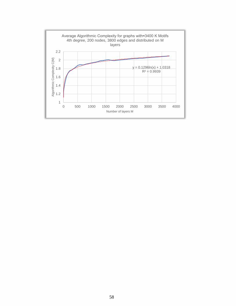
y = 0.1296ln(x) + 1.0318R² = 0.9939

1

1.2

1.4

1.6

1.8

2

2.2

0 500 1000 1500 2000 2500 3000 3500 4000

Alg

orith

mic

Com

ple

xity C

(M)

Number of layers M

Average Algorithmic Complexity for graphs with≈3400 K Motifs 4th degree, 200 nodes, 3800 edges and distributed on M

layers

59

Chapter 8

8. References

[1] Andrea Santoro and Vincenzo Nicosia, Algorithmic Complexity of

Multiplex Networks,

https://journals.aps.org/prx/abstract/10.1103/PhysRevX.10.021069

(Published 26 June 2020) [Accessed 27 January 2021]

[2] Rodney G. Downey Denis R. Hirschfeldt, Algorithmic Randomness

and Complexity,

https://books.google.se/books/about/Algorithmic_Randomness_and_Com

plexity.html?id=FwIKhn4RYzYC&printsec=frontcover&source=kp_read

_button&redir_esc=y#v=onepage&q&f=false (Springer, 29 October

2010) [Accessed 02 February 2021]

[3] Peter D. Johnson Jr., Greg A. Harris, D.C. Hankerson, Introduction to

Information Theory and Data Compression,

https://books.google.se/books?id=WFArn7VH9TcC&hl=sv&source=gbs_

navlinks_s (CRC Press, 26 February 2003) [Accessed 25 January 2021]

[4] Ming Li, Paul Vitányi An Introduction to Kolmogorov Complexity

and Its Applications (Texts in Computer Science) 4th ed.

https://www.amazon.com/Introduction-Kolmogorov-Complexity-

Applications-Computer/dp/3030112977 (Springer 2019) [Accessed 22

February 2021]

[5] A. N. Kolmogorov, On Tables of Random Numbers (Pages 387-395),

https://www.sciencedirect.com/science/article/pii/S0304397598000759?vi

a%3Dihub (Published 6 November 1998) [Accessed 22 February 2021]

[6] V Latora, V Nicosia, G Russo, Complex Networks: Principles,

Methods and Applications [1 ed.],

https://books.google.se/books/about/Complex_Networks.html?id=qV0yD

wAAQBAJ&source=kp_book_description&redir_esc=y (Cambridge

University Press 13 September 2017) [Accessed 23 February 2021]

[7] E Cozzo, G Ferraz de Arruda, FA Rodrigues, Y Moreno, Multiplex

Networks [1st ed.],

http://libgen.rs/book/index.php?md5=26F2D6EEF234441CC96AA7C223

92DA98 (Springer International Publishing 2018) [Accessed 03 Mars

2021]

[8] M. De Domenico, A. S. Sol´e-Ribalta, E. Cozzo, M. Kivelä, Y.

Moreno, M. A. Porter, S. Gómez, and A. Arenas, Mathematical

Formulation of Multilayer Networks

60

https://journals.aps.org/prx/abstract/10.1103/PhysRevX.3.041022

(Published 4 December 2013) [Accessed 20 February 2021]

[9] V Paul M.B. (2013). Conditional Kolmogorov complexity and

universal probability,

https://www.sciencedirect.com/science/article/pii/S0304397513005124

(27 August 2013, Pages 93-100) [Accessed 02 Mars 2021]

[10] https://git.savannah.gnu.org/cgit/gzip.git

[11] Norman Biggs, Discrete Mathematics (second edition), (Oxford

University press) [Accessed 10 September 2020]

[12] Jon Kleinberg, Algorithm Design,

https://www.bokus.com/bok/9781292023946/algorithm-design-pearson-

new-international-edition/ (Pearson New International Edition, 30 July

2013) [Accessed 10 November 2020]

[13] D. S. Ornstein Ergodic Theory, Randomness, and Dynamical

Systems, https://www.cambridge.org/core/journals/proceedings-of-the-

edinburgh-mathematical-society/article/d-s-ornstein-ergodic-theory-

randomness-and-dynamical-systems-yale-university-press-1975-

250/5F784A166E4559960E07984BB37D8C0A Yale University Press,

1975) [Accessed 01 Mars 2021]

[14] N Luhmann Introduction to Systems Theory,

https://www.adlibris.com/se/bok/introduction-to-systems-theory-

9780745645728 (1991) [Accessed 06 Mars 2021]

[15] Masoudi-Nejad A, Schreiber F, Razaghi MK Z (2012). "Building

Blocks of Biological Networks: A Review on Major Network Motif

Discovery Algorithms". IET Systems Biology, https://digital-

library.theiet.org/content/journals/10.1049/iet-syb.2011.0011 , (October

2012) [Accessed 01 May 2021]

[16] Uri AlonLab, Design Principles in Biology, NETWORK MOTIF

SOFTWARE, Motif dictionary,

https://www.weizmann.ac.il/mcb/UriAlon/download/network-motif-

software [Accessed 01 May 2021]

[17] S.N. Dorogovtsev and J.F.F. Mendes, Evolution of Networks: from

biological networks to the Internet and WWW,

https://oxford.universitypressscholarship.com/view/10.1093/acprof:oso/9

780198515906.001.0001/acprof-9780198515906 (Oxford University

Press, 2003) [Accessed 10 Mars 2021]

[18] B S Manoj, Abhishek Chakraborty, Rahul Singh, Complex

Networks: A Networking and Signal Processing Perspective,

https://www.pearson.com/store/p/complex-networks-a-networking-and-

61

signal-processing-perspective/P100000889947/9780134786995 (Pearson,

New York, USA, February 2018) [Accessed 1 April 2021]

[19] S Sinha, N Ganguly, A Deutsch, A Mukherjee, Dynamics on and of

Complex Networks: Applications to Biology, Computer Science, and the

Social Sciences, https://www.springer.com/gp/book/9780817647506

(Birkhäuser Basel 2009) [Accessed 10 Mars 2021]

[20] Hector Zenil, Narsis Kiani, Jesper Tegnér, Low Algorithmic

Complexity Entropy-deceiving Graphs, https://arxiv.org/abs/1608.05972

(10 May 2017) [Accessed 01 Mars 2021]

[21] H. Zenil, F. Soler-Toscano, K. Dingle and A. Louis, Correlation of

Automorphism Group Size and Topological Properties with Program-size

Complexity Evaluations of Graphs and Complex Networks,

https://www.sciencedirect.com/science/article/abs/pii/S037843711400169

1, (15 June 2014, Pages 341-358) ) [Accessed 01 Mars 2021]

[22] H. Zenil, N.A. Kiani and J. Tegnér, Methods of Information Theory

and Algorithmic Complexity for Network Biology,

https://www.sciencedirect.com/science/article/pii/S1084952116300118?c

asa_token=NDwPjhE83jEAAAAA:nwE8en9S5ynDR_-

MXdpuoxm9NyAdgWgWNJ4_A_3S2oYi4rHCvL8esvDYBWWR2pq-

zAxndXdlkhs, (Seminars in Cell and Developmental Biology, March

2016, Pages 32-43) [Accessed 01 Mars 2021]

[23] G. Bianconi, Multilayer Networks: Structure and Function (Oxford

University Press, Oxford, 2018).

[24] Definition of metaphor noun from the Oxford Advanced Learner's

Dictionary,

https://www.oxfordlearnersdictionaries.com/definition/english/metaphor?

q=metaphor

[25] S. Boccaletti, G. Bianconi, R. Criado, C. I. del Genio, J. Gómez-

Gardeñes, M. Romance, I. S. Nadal, Z. Wang, and M. Zanin, The

Structure and Dynamics of Multilayer Networks,

https://www.sciencedirect.com/science/article/pii/S0370157314002105?vi

a%3Dihub (Published 1 November 2014) [Accessed 02 Mars 2021]

[26] Rissanen, Jorma, Information and Complexity in Statistical

Modeling, https://www.springer.com/gp/book/9780387366104 (Springer

2017) [Accessed 22 April 2021]

[27] Mike James, Kolmogorov Complexity Isn't Computable ,

https://www.i-programmer.info/programming/theory/13793-

programmers-guide-to-theory-kolmogorov-

complexity.html?start=1#:~:text=Kolmogorov%20complexity%20isn't%2

0computable%20in%20the%20sense%20that%20there,complexity%20of

62

%20an%20arbitrary%20string.&text=A%20string%20that%20cannot%20

be,by%20a%20simple%20counting%20principle. (22 June 2020)

[Accessed 15 Mars 2021]

[28] G J Chaitin, ALGORITHMIC INFORMATION THEORY, Third

Printing (Cambridge University Press, Published 2 April 2003) [Accessed

15 April 2021]

[29] https://github.com/andresantoro/ALCOREM

[30] https://gits-15.sys.kth.se/kalzi/Bachelor-thesis

[31] F. Battiston, V. Nicosia, and V. Latora, Structural Measures for

Multiplex Networks,

https://journals.aps.org/pre/abstract/10.1103/PhysRevE.89.032804 (12

March 2014) [Accessed 15 Mars 2021]

[32] A Skantz and S Gateman, The Impacts of Motif Quantity on Small-

worldness in Networks, No available link.

[33] A Skantz, S Gateman, https://gits-15.sys.kth.se/solbritt/Bachelor-

thesis

[34] https://github.com/shmohammadi86/Kavosh

[35] Mean Square Error & R2 Score Clearly Explained,

https://www.bmc.com/blogs/mean-squared-error-r2-and-variance-in-

regression-analysis/, [Accessed 20 February 2021]

TRITA -EECS-EX-2021:424

www.kth.se