collaborative reliability analysis under the framework of multidisciplinary systems design

Optimization and Engineering, 6, 63–84, 2005c© 2005 Springer Science + Business Media, Inc. Manufactured in The Netherlands

Collaborative Reliability Analysis under the Frameworkof Multidisciplinary Systems Design

XIAOPING DUDepartment of Mechanical and Aerospace Engineering, University of Missouri–Rolla

WEI CHEN∗Department of Mechanical Engineering, Northwestern University, Evanston, IL 60208-3111, USAemail: [email protected]

Received July 2, 2002; Revised January 8, 2003

Abstract. Traditional Multidisciplinary Design Optimization (MDO) generates deterministic optimal designs,which are frequently pushed to the limits of design constraint boundaries, leaving little or no room to accommodateuncertainties in system input, modeling, and simulation. As a result, the design solution obtained may be highlysensitive to the variations of system input which will lead to performance loss and the solution is often risky (highlikelihood of undesired events). Reliability-based design is one of the alternative techniques for design under un-certainty. The natural method to perform reliability analysis in multidisciplinary systems is the all-in-one approachwhere the existing reliability analysis techniques are applied directly to the system-level multidisciplinary analysis.However, the all-in-one reliability analysis method requires a double loop procedure and therefore is generallyvery time consuming. To improve the efficiency of reliability analysis under the MDO framework, a collaborativereliability analysis method is proposed in this paper. The procedure of the traditional Most Probable Point (MPP)based reliability analysis method is combined with the collaborative disciplinary analyses to automatically satisfythe interdisciplinary consistency when conducting reliability analysis. As a result, only a single loop procedure isrequired and all the computations are conducted concurrently at the individual discipline-level. Compared with theexisting reliability analysis methods in MDO, the proposed method is efficient and therefore provides a cheapertool to evaluate design feasibility in MDO under uncertainty. Two examples are used for the purpose of verification.

Keywords: reliability analysis, Most Probable Point, multidisciplinary design optimization (MDO), collabora-tive design, uncertainty

1. Introduction

In designing complex engineering systems, Multidisciplinary Design Optimization (MDO)(Balling and Sobieski, 1995) has become a systematic approach to optimization of complex,coupled engineering systems, where “multidisciplinary” refers to the different aspects thatmust be included in designing a system that involves multiple interacting disciplines, such asthose found in aircraft, spacecraft, automobiles, and industrial manufacturing applications.Numerous successful examples of MDO applications have been found in many areas, suchas Electromagnetics (Makinen et al., 1999), High Speed Civil Transport Design (Walshet al., 2000a, b), Space Vehicle Design (Braun et al., 1996), Aerospike Nozzle Design (Korte

∗Corresponding author.

64 DU AND CHEN

et al., 1997), Rotor Design (Walsh et al., 1994, 1998), Integrated Controls-Structures Design(Padula et al., 1991), Integrated Circuit Design (Lokanathan et al., 1995), and AutomobileDesign (Bennet et al., 1997).

However, the traditional MDO generates deterministic optimal designs, which are fre-quently pushed to the limits of design constraint boundaries, leaving little or no room foraccommodating uncertainties in system input, modeling, and simulation. As a result, the de-sign solution obtained may be (1) highly sensitive to the variation of system input which willlead to performance loss and the solution is often risky (high likelihood of undesired events),or (2) conservative and therefore uneconomic if the deterministic safety factors are utilized.

To overcome the drawbacks of deterministic MDO, techniques for uncertainty analysisunder the MDO framework have been proposed and have been getting much attention (Duand Chen, 2000a). In recent developments, some preliminary results of multidisciplinarydesign under uncertainty are reported (Mavris et al., 1999; Koch et al., 1999; Padmanabhanand Batill, 2000; Du and Chen, 2001a, 2000a). In these works, the mean and variance ofsystem performance are evaluated through uncertainty analysis and then utilized to ob-tain optimal solutions based on robustness considerations. For example, in Du and Chen’s(2001a) work, the system uncertainty analysis (SUA) and the concurrent subsystem uncer-tainty analysis (CSSUA) methods are proposed to evaluate performance variances takinginto account the multidisciplinary design framework. In Gu’s work (Gu et al., 1998), the“worst case” concept and the first-order sensitivity analysis are used to evaluate the intervalof the end performance of a multidisciplinary system. Even though the mean, the variance,and the interval of system performance are sufficient to evaluate the robustness of a designobjective, they are generally not rigorous to be used for formulating the design feasibilityconstraints under uncertainty. The ideal formulation of the design feasibility under uncer-tainty is the use of probabilistic constraints or called reliability-based constraints whereinthe design feasibility is modeled by the probability of constraint satisfaction (reliability)(Du and Chen, 2000b); and wherein the complete shape of the performance distribution,especially that at the tail, is taken into account.

Recently, much attention has been turned to the development of procedures to couplereliability analysis and MDO (Sues et al., 1995; Sues and Cesare, 2000; Koch et al., 2000).In the work of Sues et al. (1995), response surface models of system output are createdat the system level to replace the computationally expensive simulation models. Using theresponse surface models, reliability analysis is conducted for MDO under uncertainty. Thedrawback of using their approach is the cost associated with generating an accurate responsesurface model over a large parameter space (for both deterministic and random variables).Besides, some of the response surface methods tend to “smooth” a performance behaviorand lose the information of local variations.

A framework for reliability-based MDO was proposed in Sues and Cesare (2000). Intheir work, the reliability analysis is decoupled from the optimization. Reliabilities arecomputed initially before the first execution of the optimization loop, and then updated afterthe optimization loop is executed. However, in the optimization loop, approximate formsof probabilistic constraints are used. To integrate the existing reliability analysis techniquesinto the MOD framework more tightly, a multi-stage, parallel implementation strategy ofprobabilistic design optimization was utilized by Koch et al. (2000). Nevertheless, in all

COLLABORATIVE RELIABILITY ANALYSIS 65

these existing frameworks, most computations are spent on the reliability analysis during theoptimization process. The efficiency of reliability analysis dominates the overall efficiencyof the whole design process. Since the reliability analysis in these design frameworks isusually conducted based on the system-level multidisciplinary analysis, as we will see next,two loops of iterative computations will be involved and as a result, MDO under uncertaintybecomes much less affordable compared to deterministic MDO.

To improve the efficiency of reliability analysis for MDO and eventually MDO underuncertainty, a collaborative reliability analysis method is proposed in this paper. In thismethod, the procedure of the traditional Most Probable Point (MPP) based reliability anal-ysis method is combined with the collaborative disciplinary analyses to automatically satisfythe interdisciplinary consistency in reliability analysis. As a result, only a single loop pro-cedure is required and all the computations are conducted concurrently at the individualdiscipline-level.

The paper is organized as follows. The general multidisciplinary system analysis isreviewed in Section 2. In Section 3, the strategy of the traditional all-in-one reliabilityanalysis for multidisciplinary systems is discussed and the large computational needs of thisapproach are highlighted. Our proposed collaborative reliability analysis method under theframework of multidisciplinary systems design is presented in Section 4 and two examplesare used to illustrate the effectiveness of the proposed method in Section 5. The discussionon the efficiency of the proposed method is given in Section 6. Section 7 is the closurewhich highlights the effectiveness of the proposed method and provides discussions on itsapplicability under different circumstances. It should be noted that our discussion is focusedon the reliability analysis under the optimization framework instead of the multidisciplinaryprobabilistic (reliability-based) optimization.

2. The multidisciplinary system

For simplicity, we use a 3-discipline system to present the method. The conclusions drawnbased on the 3-discipline system can be easily generalized to an n-discipline system. Figure 1

Figure 1. A multidisciplinary system.

66 DU AND CHEN

shows the 3-discipline system, where each box represents the analysis (simulation) that be-longs to a discipline. xs are the system input variables which are the input for all disciplines,also called sharing variables. xi (i = 1, 2, and 3) are the input variables of discipline i .xs and xi are mutually exclusive sets. Note that in this paper, the bold font stands for avector and a regular font stands for a scalar variable. Therefore, x represents a vector andx represents a variable or an element of vector x. In some circumstance, a bold font alsorepresents a function vector as we will see later on. yi j (i �= j) are interdisciplinary linkingvariables, which are those functional outputs calculated in discipline i , at the same time,are required as inputs to discipline j . zi are outputs of discipline i .

For discipline 1, the disciplinary input-output relations have the functional form

z1 = Fz1(xs, x1, y21, y31) (1)

y12 = Fy12(xs, x1, y21, y31) (2)

y13 = Fy13(xs, x1, y21, y31) (3)

Similarly, for disciplines 2 and 3, we have the disciplinary input-output relations

z2 = Fz2(xs, x2, y12, y32) (4)

y21 = Fy21(xs, x2, y12, y32) (5)

y23 = Fy23(xs, x2, y12, y32) (6)

and

z3 = Fz3(xs, x3, y13, y23) (7)

y31 = Fy31(xs, x3, y13, y23) (8)

y32 = Fy32(xs, x3, y13, y23) (9)

The disciplinary analysis F maps disciplinary input into disciplinary output. F can beof analytical forms or black boxes of simulation tools. F are assumed to be independentlysolvable. Taking Fz1 as an example, given appropriate inputs (xs, x1, y21, y31)for whichthe analysis is defined, we can compute the disciplinary output z1 through disciplinary 1analysis z1 = Fz1(xs, x1, y21, y31).

The coupled multidisciplinary analysis system depicted in Figure 1 reflects the phys-ical requirement that a solution simultaneously satisfies the three disciplinary analyses(Alexandrov and Lewis, 2000). We write the multidisciplinary analysis system as a simul-taneous system of equations as

y12 = Fy12(xs, x1, y21, y31)

y13 = Fy13(xs, x1, y21, y31)

y21 = Fy21(xs, x2, y12, y32)

y23 = Fy23(xs, x2, y12, y32)

y31 = Fy31(xs, x3, y13, y23)

y32 = Fy32(xs, x3, y13, y23)

(10)


Solving the coupled equation (10) leads to a full multidisciplinary analysis and we callthis analysis the system-level multidisciplinary analysis, or simply system-level analysis, inwhich the coupled disciplines give a physically consistent result.

Without the consideration of uncertainty, a general MDO model is simplified as:

min f (xs, z′1, z′

2, z′3)

s.t. z′′1(xs, x1, y21, y31) ≥ 0

(11)z′′

2(xs, x2, y12, y32) ≥ 0

z′′3(xs, x3, y13, y23) ≥ 0

where f is the collaborative design objective, representing the function of system designvariables xs and subsystem performance z′

i (i = 1, 2 and 3) which are part of the output z ofdiscipline i . z′′

i (i = 1, 2 and 3) stand for those subsystem performance that are consideredas design constraints.

In many engineering problems, randomness is associated with system input variablesxs and disciplinary input variables xi . Examples of the randomness include the randommaterial properties, manufacturing tolerances, and stochastic loads and stochastic operationenvironments, which can be described by probabilistic distributions. Since the output zi

(i = 1, 2 and 3) are functions of random input variables xs and disciplinary input variablesxi , zi = {z′

i , z′′i } are also random variables. For the same reason, all the linking variables

yi j are also random variables. This phenomenon rouses the issue of reliability which isconcerned with how to assess the design feasibility z′′

i ≥ 0.

3. All-in-one reliability analysis method for MDO

With the existence of uncertainty, the deterministic MDO model (11) is reformulated as

min f (xs, z′1, z′

2, z′3)

s.t. P{z′′1(xs, x1, y21, y31) ≥ 0} ≥ P1 (12)

P{z′′2(xs, x2, y12, y32) ≥ 0} ≥ P2

P{z′′3(xs, x3, y13, y23) ≥ 0} ≥ P3

The design feasibility under uncertainty is represented probabilistically such that theprobability of the constraint satisfaction z′′

i ≥ 0 is greater than or equal to the desiredprobability Pi . The probability of the constraint satisfaction can also be called the reliability.As we will discuss next, the reliability assessment is a critical component that demands muchmore computational effort for MDO under uncertainty than deterministic MDO. Efficientreliability analysis methods are therefore needed to suit the need of MDO. To explain theall-in-one reliability analysis method, we need to first explain the concept of reliability andthe Most Probable Point (MPP) method.

For simplicity of discussion, in this section we use z (a scalar) to represent any element ofthe disciplinary system output vector z′′

i , x to represent all the inputs of disciplinary analysis

68 DU AND CHEN

Figure 2. Limit state concept.

(including linking variables as the input of discipline i), and F to represent the disciplinaryanalysis corresponding to z. For example, if we are interested in the reliability associatedwith one element z1 out of the disciplinary output vector z′′

1, we then use z = z1, x =(xs, x1, y21, y31), and F = Fz1. Therefore, disciplinary output of interest has a functionalrelationship z = F(x). In the reliability field, z = F(x) characterizes the function of aspecific performance criterion z and is called a limit state function. The failure surface orthe limit state is defined as F(x) = c or simply F(x) = 0. This is the boundary between thesafe and the failure regions in the random variables space. When F(x) > 0, the system (orthe discipline) is considered safe and when F(x) < 0, the system can no longer fulfill thefunction for which it was designed. Figure 2 shows the limit state for a two dimensionalproblem. Both x1 and x2 are random design variables.

The probability of failure p f is defined as the probability of the event that the system canno longer fulfill its function and p f is given by

p f = P{F(x) < 0} (13)

which is generally calculated by the integral

p f =∫

· · ·∫

F(x)<0fx(x)dx (14)

where fx(x) is the joint probability density function (PDF) of x and the probability isevaluated by the multidimensional integration over the failure region F(x).

The reliability R is the probability that the system functions properly and it is givenby

R = P{F(x) > 0} = 1 − p f (15)

It is very difficult or even impossible to analytically compute the multidimensional inte-gration in (14). An alternative method to evaluate the integration is Monte Carlo simulation(Habitz, 1986). However, when the probability of failure p f is very small or the reliability


is very high (close to 1), the computational effort of Monte Carlo Simulation is extremelyexpensive (this will be demonstrated by the examples in Section 5). To overcome this diffi-culty, Hasofer and Lind (1974) proposed the concept of the Most Probable Point (MPP) toapproximate the integration.

To make use of the MPP concept, the input random variables x = {x1, x2, . . . , xn}(inthe original design space, x–space) are transformed into an independent and standardizednormal space u = {u1, u2, . . . , un}(u–space). The most commonly used transformation isgiven by Rosenblatt (Rosenblatt, 1952) as

ui = Φ−1[Gi (xi )] (i = 1, . . . , n), (16)

where �−1 is the inverse of a normal distribution and Gi is the cumulative distributionfunction (CDF) of xi . (16) implies that the transformation maintains the CDFs being identicalboth in x-space and u-space.

The limit state function is now rewritten as

F(x) = F(u) = 0 (17)

To easily assess reliability, Hasofer and Lind (1974) used the safety index β which isdefined as the shortest distance from the origin to a point on the limit-state surface in u-space(Figure 3). Searching for β can be formulated as a minimization problem with an equalityconstraint:

{β = min

U(uT u)1/2

subject to F(u) = 0(18)

The solution of this minimization problem uMPP is called the Most Probable Point (MPP).From Figure 3, we see that the joint probability density function on the limit state surface

Figure 3. The MPP concept.

70 DU AND CHEN

has its highest value at the MPP and therefore the MPP has the property that in the standardnormal space it has the highest probability of producing the value of limit state functionF(u) or highest contribution to the integral (14) (Wu, 1990).

If the limit-state function F(u) is linear, the accurate probability estimate at the limit stateis given by the equation:

p f = P{F(x) < 0} = 1 − �(β). (19)

The above equation provides an easy correspondence between the failure probability esti-mate and the safety index or the shortest distance β. Since (19) only utilizes the first orderderivative of the limit state function, the method is called the First Order Reliability Method(FORM). Higher-order adjustments can be adopted if the magnitude of the principal curva-tures of the limit-state surface in the u-space at the MPP is large(Mitteau, 1999). Besides using optimization algorithms to solve problem (18), there existmany other MPP searching algorithms (Khalessi et al., 1991; Wu, 1990, 1998; Du and Chen,2000c).

If the MPP based method applied directly to integrated multidisciplinary systems toevaluate the reliability, we call this approach all-in-one reliability analysis. In the fol-lowing, we use one output of discipline 1, z1, as an example to present the method andillustrate the huge computational effort associated with this approach . Here, we expectto evaluate the probability of failure (design feasibility) in discipline 1 and this is givenby

p f = P{z1 = Fz1(x) < 0} = P{Fz1(xs, x1, y21, y31) < 0} (20)

For the case of the multidisciplinary system as shown in (20), since the distributions ofinputs y21 and y31 (linking variables) are not known within the scope of discipline 1, weneed to perform the system-level analysis to solve the linking variables y21 and y31, andeventually, the limit state function Fz1 becomes the function of system inputs (xs, x1, x2, x3).Hence

p f = P{Fz1(x) < 0} = P{Fz1(xs, x1, x2, x3) < 0} (21)

Based on Eq. (21), the mathematical model to find the MPP is formulated as

Minimize β = (uT u)12

DV = u = (us, u1, u2, u3) (22)

Subject to z1 = Fz1(us, u1, u2, u3) = 0

DV—design variables

where us, u1, u2, and u3 are random variables in u-space corresponding to random designvariables xs, x1, x2, and x3 in x-space.


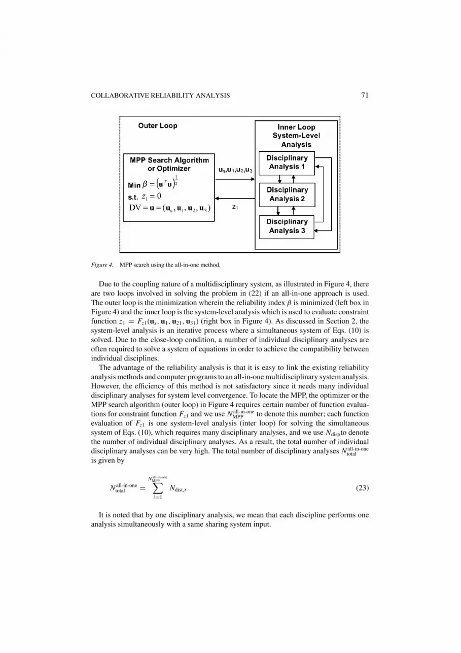
Figure 4. MPP search using the all-in-one method.

Due to the coupling nature of a multidisciplinary system, as illustrated in Figure 4, thereare two loops involved in solving the problem in (22) if an all-in-one approach is used.The outer loop is the minimization wherein the reliability index β is minimized (left box inFigure 4) and the inner loop is the system-level analysis which is used to evaluate constraintfunction z1 = Fz1(us, u1, u21, u31) (right box in Figure 4). As discussed in Section 2, thesystem-level analysis is an iterative process where a simultaneous system of Eqs. (10) issolved. Due to the close-loop condition, a number of individual disciplinary analyses areoften required to solve a system of equations in order to achieve the compatibility betweenindividual disciplines.

The advantage of the reliability analysis is that it is easy to link the existing reliabilityanalysis methods and computer programs to an all-in-one multidisciplinary system analysis.However, the efficiency of this method is not satisfactory since it needs many individualdisciplinary analyses for system level convergence. To locate the MPP, the optimizer or theMPP search algorithm (outer loop) in Figure 4 requires certain number of function evalua-tions for constraint function Fz1 and we use N all-in-one

MPP to denote this number; each functionevaluation of Fz1 is one system-level analysis (inter loop) for solving the simultaneoussystem of Eqs. (10), which requires many disciplinary analyses, and we use Ndispto denotethe number of individual disciplinary analyses. As a result, the total number of individualdisciplinary analyses can be very high. The total number of disciplinary analyses N all-in-one

totalis given by

N all-in-onetotal =

N all-in-oneMPP∑i=1

Ndist,i (23)

It is noted that by one disciplinary analysis, we mean that each discipline performs oneanalysis simultaneously with a same sharing system input.

72 DU AND CHEN

To improve the efficiency of reliability analysis for multidisciplinary systems, we proposea collaborative reliability analysis method which does not require any system-level analysisand significantly reduces the number of individual disciplinary analyses. The proposedmethod will be presented in detail in the next section and demonstrative examples will begiven in Section 6.

4. The collaborative reliability analysis for multidisciplinary systems

To reduce the total number of system level and subsystem (disciplinary) level analyses,we use a single loop strategy for reliability analysis under the MDO framework. The opti-mization loop for MPP search and the iterative system-level multidisciplinary analysis arecombined to avoid the nested loops. The compatibility conditions among multiple disci-plines are formulated as constraint functions in the optimization model for MPP search.By doing this, there is no need for maintaining the compatibility among disciplines in eachfunction evaluation during the MPP search process. This treatment is different from theexisting all-in-one reliability analysis method. The compatibility will be achieved progres-sively in the optimization process for MPP search and will be satisfied eventually at thelocated MPP.

For the same problem presented in last section, the MPP searching problem is reformu-lated as


DV = {u, y12, y13, y21, y23, y31, y32} and u = (us, u1, u2, u3)

Subject to z1 = Fz1(us, u1, y21, y31) = 0 (Discipline analysis 1)

y12 − Fy12(us, u1, y21, y31) = 0 (Discipline analysis 1)

y13 − Fy13(us, u1, y21, y31) = 0 (Discipline analysis 1)(24)





DV—design variables

The first equality constraint is the limit state function at its limit state. The remainingequality constraints stand for the interdisciplinary consistency conditions in (10). All thelinking variables yi j are also included as part of decision variables (DV). It should be notedthat all the linking variables need to be transformed into u-space. The proposed strategyis illustrated in Figure 5 from which we see that the optimization for MPP search in-teracts with individual subsystem analyses separately but there are no direct interactionsamong subsystems. Taking discipline 1 as an example, the optimizer (for MPP search)passes the decision variables y21 and y31 (linking variables), as well as us (corresponding to


Figure 5. MPP search in collaborative reliability analysis.

system variables xs) and u1 (corresponding to disciplinary variables x1) to discipline 1. Thedisciplinary analysis 1 is executed to compute a part of its outputs Fy12(us, u1, y21, y31)and Fy13(us, u1, y21, y31 which will serve as inputs of disciplines 2 (y12) and 3 (y13), re-spectively. To maintain the interdisciplinary compatibility, the equality constraints are setas y12 − Fy12(us, u1, y21, y31) = 0 and y31 − Fy13(us, u1, y21, y31) = 0 for discipline 1.Disciplines 2 and 3 work in the same way.

It is noted that with the proposed method, in the process of searching the MPP, onlyindividual disciplinary analyses are required and no system-level multidisciplinary anal-ysis is needed. All disciplinary analyses can be conducted concurrently which facilitatesparellization. Since only one loop (the optimization loop for MPP search) is involved foriterative disciplinary analyses, compared with the all-in-one reliability analysis method,the collaborative reliability analysis method in general needs much less disciplinary anal-yses and hence is more efficient. To verify this, a detailed discussion is given in nextsection.

5. Theoretical verification of the improved efficiency

From the previous discussions, we see that the all-in-one reliability analysis method requiresa double-loop procedure and the collaborate reliability analysis method requires a single-loop procedure. This indicates that the collaborate reliability analysis method could be moreefficient than the all-in-one reliability analysis method. In the following, we will discussin principle why the proposed collaborative reliability analysis method is generally moreefficient than the all-in-one reliability analysis method. For the collaborative reliabilityanalysis method, let the total number of disciplinary analyses for each reliability analysisbeN collaborative

total , which is equal to the number of function evaluations N collaborateMPP for solving

74 DU AND CHEN

the optimization formulation (24) in MPP search, i.e.,

N collaborativetotal = N collaborative

MPP (25)

For the all-in-one reliability analysis method, For the all-in-one reliability analysismethod, let the average number of disciplinary analyses for a function evaluation in theouter optimization loop of MPP search be N disp, then the total number of disciplinaryanalyses of all-in-one reliability analysis method in (23) is rewritten as

N all-in-onetotal = N all-in-one

MPP Ndisp (26)

and usually N disp � 1(� means much greater than).When the directives of system functions are evaluated numerically for solving the MPP

search optimization problem, for example, by the finite difference method, the numbers offunction evaluations in MPP search for both methods are approximately proportional to thenumber of unknown variables in MPP search, therefore,

N all-in-oneMPP = N all-in-one

iter

(Nx + Call-in-one

)(27)

and

N collaborativeMPP = N collaborative

iter

(Nx + Ny + Ccollaborative

)(28)

where Nx is the number of random system input variables (including input variables for thediscipline and the sharing input variables) and Ny is the total number of linking variables.C is the average number of function evaluations for other purposes (other than derivativeevaluations), for instance, for calculations of function value at current iteration, and for theone-dimensional search (line or arc search) when implementing an optimization algorithm.Niter is the number of iterations in the optimization for MPP search.

From (25) through (28), the total numbers of disciplinary analyses are


iter

(Nx + Call-in-one

)N disp (29)

and


iter

(Nx + Ny + Ccollaborative

)(30)

In general, the number of iterations N all-in-oneiter �= N collaborative

iter and Call-in-one �= Ccollaborative,and it is difficult to conclude rigorously which method needs more disciplinary analyses.However, we can roughly compare both methods based on Eqs. (29) and (30).

Usually, the number of iterations N all-in-oneiter and N collaborative

iter are of the same order ofmagnitude and so are Call-in-one and Ccollaborative. If the number of linking variables is notmuch greater than the number of input variables, Nx and Nx + Nyare also of the same


order of magnitude. Since N disp is much greater than one, from Eqs. (29) and (30), we mayconclude that N all-in-one

total is much greater than N collaborativetotal . Based on the above reasoning,

the proposed collaborative reliability analysis method should be more efficient than theall-in-one reliability analysis method.

In the case that the number of linking variables Ny is much larger than the number of inputvariables Nx , which is rare in practical applications, the collaborative reliability analysismethod may not be as efficient as the all-in-one reliability analysis method. However,if computational parallelization is utilized, the collaborative method could still be morefavorable.

When the derivatives are evaluated analytically, Nx = Ny = 0, Eqs. (29) and (30) become


iter Call-in-one N disp (31)

and


iter Ccollaborative (32)

Since in general, the number of iterations N all-in-oneiter and N collaborative

iter are of the same orderof magnitude and so are Call-in-one and Ccollaborative, and N disp is much greater than one,we conclude that N all-in-one

total is much greater than N collaborativetotal . Therefore, the collaborative

reliability analysis method is more efficient than the all-in-one reliability analysis methodwhen analytical differentiations are used.

Providing a strict mathematical proof of the efficiency of the proposed method is verydifficult or even impossible because the number of function evaluations of the MPP searchand the number of disciplinary analyses for a system-level analysis cannot be preciselyobtained (the numbers vary problem by problem). However, from the discussion above,we are able to understand in principle, why the proposed collaborative reliability analysismethod is more efficient than the all-in-one method in general and what are the exceptions.We will further verify this by examples in the next section.

6. Examples

Two examples are used to illustrate the effectiveness of our proposed reliability analysistechnique under the framework multidisciplinary systems design. These two examples havebeen used in (Du and Chen, 2001a) to demonstrate the moment matching method forrobust multidisciplinary design optimization where only the first two moments (the meanand the variance) of system performance are generated. We use these examples hereinagain for more rigorous formulation under uncertainty (reliability analysis). To verify ourproposed method, we consider two aspects, namely, efficiency and accuracy. For efficiency,we compare the total number of individual disciplinary analyses needed for the proposedmethod with those for the all-in-one reliability analysis method. For accuracy, results fromMonte Carlo Simulations with sufficient simulation sizes are considered as the referencesolution for confirmation. The sequential quadratic programming (SQP) is used as the

76 DU AND CHEN

Figure 6. Example 1.

optimization search algorithm to locate the MPP in both collaborative reliability analysisand all-in-one reliability analysis. Our illustration again is focused on reliability analysisinstead of probabilistic optimization.

Example 1. A multidisciplinary system is composed of two disciplines as shown inFigure 6.

For discipline 1, the functional relationships are represented as

xs = {x1}, x1 = {x2, x3}, y1 = y12 = {y12}, z1 = {z1} (33)

Fy12(xs, x1, y21) = Fy12(x1, x2, x3, y21) = x21 + 2x2 − x3 + 2

√y21 (34)

Fz1(xs, x1, y21) = Fz1(x1, x2, x3, y21) = c − (x2

1 + 2x2 + x3 + x2e−y21)

(35)

where c is a constant.For discipline 2, the functional relationships are represented as

xs = {x1}, x2 = {x4, x5}, y2 = y21 = {y21}, z2 = {z2} (36)

Fy21(xs, x2, y12) = Fy21(x1, x4, x5, y12) = x1x4 + x24 + x5 + y12 (37)

Fz2(xs, x2, y12) = Fz2(x1, x4, x5, y12) = √x1 + x4 + x5(0.4x1) (38)

It is assumed that all the random variables x are normally distributed. The coefficient ofvariation (COV) of all the random variables is 0.1. The COV is the ratio of the standarddeviation to the mean value.

Two design points are arbitrarily chosen for reliability analysis. At design point 1 wherethe mean values of x = (x1, x2, x3, x4, x5) are µx = (1, 1, 1, 1, 1), the limit state functionis considered with c = 5, namely

Fz1 = 5 − (x2

1 + 2x2 + x3 + x2e−y21)

(39)


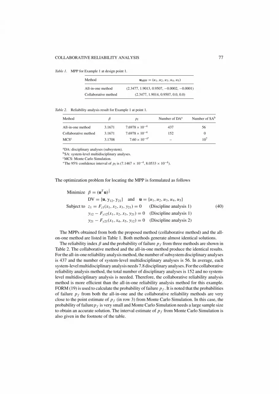
Table 1. MPP for Example 1 at design point 1.

Method uMPP = (u1, u2, u3, u4, u5)

All-in-one method (2.3477, 1.9013, 0.9507, −0.0002, −0.0001)

Collaborative method (2.3477, 1.9014, 0.9507, 0.0, 0.0)

Table 2. Reliability analysis result for Example 1 at point 1.

Method β pf Number of DAa Number of SAb

All-in-one method 3.1671 7.6978 × 10−4 437 56

Collaborative method 3.1671 7.6978 × 10−4 152 0

MCSc 3.1708 7.60 × 10−4∗– 107

aDA: disciplinary analyses (subsystem).bSA: system-level multidisciplinary analyses.cMCS: Monte Carlo Simulation.∗The 95% confidence interval of pf is (7.1467 × 10−4, 8.0533 × 10−4).

The optimization problem for locating the MPP is formulated as follows


DV = {u, y12, y21} and u = {u1, u2, u3, u4, u5}Subject to z1 = Fz1(x1, x2, x3, y21) = 0 (Discipline analysis 1) (40)

y12 − Fy12(x1, x2, x3, y21) = 0 (Discipline analysis 1)

y21 − Fy21(x1, x4, x5, y12) = 0 (Discipline analysis 2)

The MPPs obtained from both the proposed method (collaborative method) and the all-on-one method are listed in Table 1. Both methods generate almost identical solutions.

The reliability index β and the probability of failure p f from three methods are shown inTable 2. The collaborative method and the all-in-one method produce the identical results.For the all-in-one reliability analysis method, the number of subsystem disciplinary analysesis 437 and the number of system-level multidisciplinary analyses is 56. In average, eachsystem-level multidisciplinary analysis needs 7.8 disciplinary analyses. For the collaborativereliability analysis method, the total number of disciplinary analyses is 152 and no system-level multidisciplinary analysis is needed. Therefore, the collaborative reliability analysismethod is more efficient than the all-in-one reliability analysis method for this example.FORM (19) is used to calculate the probability of failure p f . It is noted that the probabilitiesof failure p f from both the all-in-one and the collaborative reliability methods are veryclose to the point estimate of p f (in row 3) from Monte Carlo Simulation. In this case, theprobability of failurep f is very small and Monte Carlo Simulation needs a large sample sizeto obtain an accurate solution. The interval estimate of p f from Monte Carlo Simulation isalso given in the footnote of the table.

78 DU AND CHEN

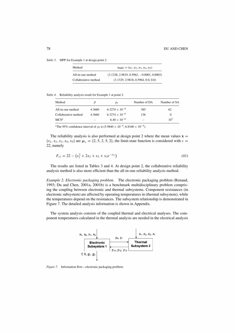
Table 3. MPP for Example 1 at design point 2.

Method uMPP = (u1, u2, u3, u4, u5)

All-in-one method (3.1328, 2.9819, 0.5962, −0.0001, 0.0003)

Collaborative method (3.1329, 2.9818, 0.5964, 0.0, 0.0)

Table 4. Reliability analysis result for Example 1 at point 2.

Method β pf Number of DA Number of SA

All-in-one method 4.3660 6.3274 × 10−6 385 62


MCSa – 6.40 × 10−6 – 107

aThe 95% confidence interval of pf is (5.9840 × 10−4, 6.8160 × 10−4).

The reliability analysis is also performed at design point 2 where the mean values x ={x1, x2, x3, x4, x5} are µx = {2, 5, 2, 5, 2}, the limit-state function is considered with c =22, namely

Fz1 = 22 − (x2

1 + 2x2 + x3 + x2e−y21)

(41)

The results are listed in Tables 3 and 4. At design point 2, the collaborative reliabilityanalysis method is also more efficient than the all-in-one reliability analysis method.

Example 2. Electronic packaging problem. The electronic packaging problem (Renaud,1993; Du and Chen, 2001a, 2001b) is a benchmark multidisciplinary problem compris-ing the coupling between electronic and thermal subsystems. Component resistances (inelectronic subsystem) are affected by operating temperatures in (thermal subsystem), whilethe temperatures depend on the resistances. The subsystem relationship is demonstrated inFigure 7. The detailed analysis information is shown in Appendix.

The system analysis consists of the coupled thermal and electrical analyses. The com-ponent temperatures calculated in the thermal analysis are needed in the electrical analysis

Figure 7. Information flow—electronic packaging problem.


in order to compute the power dissipation of each resistor. Likewise, the power dissipa-tion of each component must be known in order for the thermal analysis to compute thetemperatures.

There are eight random input variables x1– x8, five linking variables y6, y7, y11, y12, y13,and four system outputs f , h, g1 and g2.

The sets of variables and functions in the two subsystems are shown as follows, where{φ} stands for an empty set.

Electronic disciplinary analysis:

Input variables: xs = {φ}, x1 = {x5, x6, x7, x8}Linking variables: y21 = {y6, y7}Outputs: z1 = { f, h, g1, g2}

Thermal disciplinary analysis:

Input variables: xs = {φ}, x2 = {x1, x2, x3, x4}Linking variables: y12 = {y11, y12, y13}Outputs: z2 = {φ}

Of the two subsystems, the thermal analysis is more complex, which requires a finitedifference solution for the temperature distribution calculation. The remaining equations inthe thermal subsystem are solved algebraically. All equations of the electrical system aresolved algebraically.

g1 and g2 are considered as the limit state functions, which are the differences of the com-ponent temperature and the allowable temperature. We assume uncertainties are associatedwith the input variables xi (i = 1, . . . , 8), described by normal distributions. The variationcoefficient (the ratio of the standard deviation over the mean) of xi is 0.1.

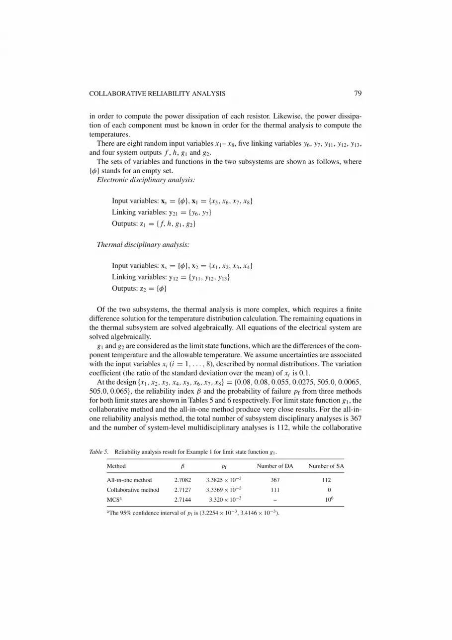
At the design {x1, x2, x3, x4, x5, x6, x7, x8} = {0.08, 0.08, 0.055, 0.0275, 505.0, 0.0065,

505.0, 0.065}, the reliability index β and the probability of failure pf from three methodsfor both limit states are shown in Tables 5 and 6 respectively. For limit state function g1, thecollaborative method and the all-in-one method produce very close results. For the all-in-one reliability analysis method, the total number of subsystem disciplinary analyses is 367and the number of system-level multidisciplinary analyses is 112, while the collaborative

Table 5. Reliability analysis result for Example 1 for limit state function g1.


All-in-one method 2.7082 3.3825 × 10−3 367 112


MCSa 2.7144 3.320 × 10−3 – 106


80 DU AND CHEN

Table 6. Reliability analysis result for Example 1 for limit state function g1.


All-in-one method 3.0779 1.0 × 10−3 531 164


MCSa 3.0357 1.15 × 10−3 – 106


reliability analysis method uses only 111 subsystem disciplinary analyses and zero system-level multidisciplinary analysis. In this sense, the collaborative reliability analysis methodis more efficient than the all-in-one reliability analysis method. FORM is used to calculatethe probability of failure pf. It is noted that the probabilities of failure pf from both the all-in-one and the collaborative reliability methods are very close to the one from Monte CarloSimulation. For limit state function g2, we have the similar conclusion. The collaborativemethod requires only 169 subsystem disciplinary analyses while 531 disciplinary analysesare used by the all-in-one method.

7. Concluding remarks

In the traditional all-in-one reliability analysis method, the optimizer for locating the MPPrepeatedly calls the limit state function which is evaluated at system-level wherein a numberof individual disciplinary analyses are performed. Two nested loops are therefore involvedin an all-in-one reliability analysis. The outer loop is the minimization problem for MPPsearch and the inner loop is the system-level analysis. The number of design variables ofthe minimization problem of an all-in-one reliability analysis is equal to the total number ofrandom system input variables and random disciplinary input variables for all disciplines.

In contrast with the all-in-one reliability analysis, the collaborative reliability analysismethod developed in this paper only employs a single optimization loop for MPP search.The interdisciplinary consistency (the system of simultaneous equations) is embedded in theoptimization model for MPP search as equality constraints. In the process of searching theMPP, the interdisciplinary consistency is satisfied progressively. By this way, computationscan be conducted concurrently at the individual disciplinary level. The design variablesin the optimization for locating the MPP are random system input variables and randomdisciplinary input variables for all disciplines, as well as all the linking variables. Eventhough larger number of design variables (the difference is the total number of linkingvariables) may lead to more function evaluations in MPP search, the overall efficiency ofthe collaborative reliability analysis is generally superior to the all-in-one reliability analysisas discussed in principle in Section 5 and demonstrated by the two examples in Section 5due to the single loop procedure.

As for accuracy, both methods generally produce the same reliability estimations sinceboth are based on the MPP concept for reliability assessment. It should be noted that be-sides the consideration of efficiency, depending on the existing computational framework


for multidisciplinary analyses, one or the other method could be more favored. For instance,with the all-in-one reliability analysis, it is easier to integrate the existing reliability anal-ysis methods/programs with an MDO framework where multidisciplinary analyses havebeen integrated at the system level. With the collaborative reliability analysis method, theoptimization problem for MPP search with interdisciplinary consistency needs to be cus-tomized by a designer. However, the collaborative reliability analysis method could bemore favored under a distributed computing environment. It should also be noted that bothmethods in principle are gradient based and therefore the computational effort is approxi-mately proportional to the number of random input variables (as well as linking variablesfor the collaborative method). With extremely high problem dimensions, the Monte CarloSimulation can be considered as an alternative (Du and Chen, 2001b).

The proposed method is demonstrated in this paper only for the purpose of reliabilityanalysis under the MDO framework. When we perform MDO under uncertainty, for ex-ample, robust MDO and reliability-based MDO, the techniques discussed herein can beutilized to evaluate any probabilistic objectives and probabilistic constraints. For MDO un-der uncertainty, the reliability analysis is called repeatedly by the MDO optimizer. In otherwords, the reliability analysis loop will be embedded in the optimization loop of the MDO.If the all-on-one reliability analysis method is adopted, the procedure of an MDO becomes atriple-loop. As a result, the computation will be prohibitively expensive. However, if we usethe proposed collaborative reliability analysis method, only two-loop procedure is neededand therefore the computational burden is mitigated.

No matter which reliability analysis method is employed, evaluating probabilistic con-straint directly under MDO optimizer always introduces nested loops. As a part of thefuture work, we plan to develop more efficient strategies and methods, ideally, single-loopstrategy, to suit the features of probabilistic design under the MDO environment.

Appendix: Analytical relationships in the electronic packaging design

Input variables are:x1: The electronic packaging problem:x2: Heat sink width (m)x3: Heat sink length (m)x4: Fin length (m)x5: Fin width (m)x6: Resistance #1 at temperature T◦ (�)x7: Temperature coefficient of electrical resistance #1 (◦K−1)x8: Resistance #2 at temperature #2 (◦K−1)

The thermal and electrical state variables (linking variables) are:y1: negative of watt density (watts/m3)y2: resistance #1 at temperature T◦

1 (�)y3: resistance #1 at temperature T◦

2 (�)y4: current in resistor #1 (amps)y5: current in resistor #2 (amps)y6: power dissipation in resistor #1 (watts)

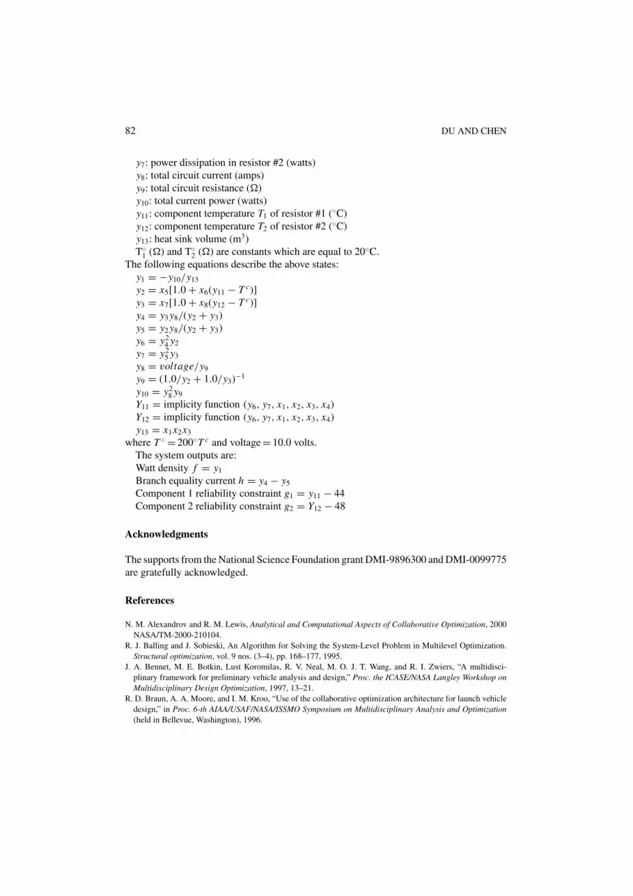
82 DU AND CHEN

y7: power dissipation in resistor #2 (watts)y8: total circuit current (amps)y9: total circuit resistance (�)y10: total current power (watts)y11: component temperature T1 of resistor #1 (◦C)y12: component temperature T2 of resistor #2 (◦C)y13: heat sink volume (m3)T◦

1 (�) and T◦2 (�) are constants which are equal to 20◦C.

The following equations describe the above states:y1 = −y10/y13

y2 = x5[1.0 + x6(y11 − T c)]y3 = x7[1.0 + x8(y12 − T c)]y4 = y3 y8/(y2 + y3)y5 = y2 y8/(y2 + y3)y6 = y2

4 y2

y7 = y25 y3

y8 = voltage/y9

y9 = (1.0/y2 + 1.0/y3)−1

y10 = y28 y9

Y11 = implicity function (y6, y7, x1, x2, x3, x4)Y12 = implicity function (y6, y7, x1, x2, x3, x4)y13 = x1x2x3

where T ◦ = 200◦T c and voltage = 10.0 volts.The system outputs are:Watt density f = y1

Branch equality current h = y4 − y5

Component 1 reliability constraint g1 = y11 − 44Component 2 reliability constraint g2 = Y12 − 48

Acknowledgments

The supports from the National Science Foundation grant DMI-9896300 and DMI-0099775are gratefully acknowledged.

References

N. M. Alexandrov and R. M. Lewis, Analytical and Computational Aspects of Collaborative Optimization, 2000NASA/TM-2000-210104.

R. J. Balling and J. Sobieski, An Algorithm for Solving the System-Level Problem in Multilevel Optimization.Structural optimization, vol. 9 nos. (3–4), pp. 168–177, 1995.

J. A. Bennet, M. E. Botkin, Lust Koromilas, R. V. Neal, M. O. J. T. Wang, and R. I. Zwiers, “A multidisci-plinary framework for preliminary vehicle analysis and design,” Proc. the ICASE/NASA Langley Workshop onMultidisciplinary Design Optimization, 1997, 13–21.

R. D. Braun, A. A. Moore, and I. M. Kroo, “Use of the collaborative optimization architecture for launch vehicledesign,” in Proc. 6-th AIAA/USAF/NASA/ISSMO Symposium on Multidisciplinary Analysis and Optimization(held in Bellevue, Washington), 1996.


X. Du, and W. Chen, “An integrated methodology for uncertainty propagation and management in simulation-basedsystems design,” AIAA Journal, vol. 38, pp. 1471–1478, 2000a.

X. Du and W. Chen, “Towards a better understanding of modeling feasibility robustness in engineering,” ASMEJournal of Mechanical Design, vol. 122, pp. 357–583, 2000b.

X. Du and W. Chen, “A most probable point based method for uncertainty analysis,” Journal of Design andManufacturing Automation. vol. 4, pp. 47–66, 2000c.

X. Du and W. Chen, “Efficient uncertainty analysis methods for multidisciplinary robust design,” in AIAA Journal.To appear 2001a.

X. Du and W. Chen, “A hierarchical approach to collaborative multiobjective robust design,” in Proc. 4-th Congressof Structural and Multidisciplinary Optimization (help in Dalin, China), 2001b.

X. Gu, J. E. Renaud, and S. M. Batill, “An Investigation of Multidisciplinary Design Subject to Uncertainties,”in Proc. of 7-th AIAA/USAF/NASA/ISSMO Multidisciplinary Analysis & Optimization Symposium (held in St.Louise, Missouri) 1998, pp. 309–319.

A. Harbits, An efficient sampling method for probability of Failure calculation,” Structure Safety, vol. 3, no.(3),pp. 109–115, 1986.

A. M. Hasofer and N. C. Lind, “Exact and invariant second-moment code format,” Journal of the EngineeringMechanics Division, vol. 100, pp. 111–121, 1974.

M. R. Khalessi, Y.-T. Wu, and T. Y. Torng, “Most-probable-point-locus reliability method in standard normal,” in9th Biennial Conference on Reliability, Stress Analysis, and Failure Prevention presented at the 1991 ASMEDesign Technical Conferences (held in Miami, FL), 1991.

P. K. Koch, B. Wujek, and O. Golovidov “A multi-stage, parallel implementation of probabilistic design opti-mization in an MDO framework,” in Proc. the 8-th AIAA/USAF/NAS/ISSMO Symposium on MultidisciplinaryAnalysis and Optimization, (held in Long Beach, CA), 2000.

P. N. Koch, T. W. Simpson, J. K. Allen, and F. Mistree “Statistical approximations for multidisciplinary designoptimization: The problem of size,” Journal of Aircraft, vol. 36, no. 1, pp. 275–286, 1999.

J. J. Korte, A. O. Salas, H. J. Dunn, N. Alexandrov, W. Follett, G. Orient, and A. Hadid, Multidisciplinary Approachto Aerospike Nozzle Design, 1997, NASA TM-110326.

N. Lokanathan, J. B. Brockman, and J. E. Renaud, “A multidisciplinary optimization approach to integratedcircuit design,” in Proc. of Concurrent Engineering: A Global Perspective, CE95 Conference (held in McLean,Virginia), 1995, pp. 121–129.

R. A. E. Makinen, J. Periaux, and J. Toivanen, “Multidisciplinary shape optimization in aerodynamics and elec-tromagnetics using genetic algorithms,” International Journal for Numerical Methods in Fluids, vol. 30,pp. 149–159, 1999.

D. V. Mavris, O. Bandte, and D. A. DeLaurentis, “Robust design simulation: A probabilistic approach to multi-disciplinary design,” Journal of Aircraft, vol. 36, no. 1, pp. 298–397, 1999.

J.-C. Mitteau, “Error evaluations for the computation of failure probability in static structural reliability problems,”Probabilistic Engineering Mechanics, vol. 14, pp. 119–135, 1999.

D. Padmanabhan and S. M. Batill “An iterative concurrent subspace robust design framework,” in Proc. of 8-thAIAA/USAF/NASA/ISSMO Symposium on Multidisciplinary Analysis and Optimization (held in Long Beach,California), 2000.

S. L. Padula, B. B. James, P. C Graves, and S. E. Woodard, Multidisciplinary Optimization of Controlled SpaceStructures With Global Sensitivity Equations. 1991, NASA TP-3130.

J. E. Renaud, An optimization strategy for multidisciplinary systems design. in 9th International conference onengineering design, Heurista, 1993, pp. 65–174.

M. Rosenblatt, “Remarks on a multivariate transformation,” Annal of Mathematical Statistics, vol. 23, pp. 470–472, 1952.

R. H. Sues and M. A. Cesare, “An innovative framework for reliability-based MDO,” in Proc. of the 41stAIAA/ASME/ASCE/AHS/ASC Structures, Structural Dynamics and Materials Conference (held in Atlanta, GA),2000.

R. H. Sues, D. R. Oakley, and G. S. Rhodes, Multidisciplinary stochastic optimization. in Proc. of the 10-thConference on Engineering Mechanics (held in Boulder), 1995 Part 2, Vol. 2, pp. 934–937.

J. L. Walsh, J. C. Townsend, A. O. Salas, J. A. Samareh, V. Mukhopadhyay, and J-F. Barthelemy, “MultidisciplinaryHigh-fidelity analysis and optimization of aerospace vehicles,” Part I: Formulation. in Proc. of the 38-th AIAA

84 DU AND CHEN

Aerospace Sciences Meeting and Exhibit (held in Reno, Nevada), 2000a.J. L. Walsh, R. P. Weston, J. A. Samareh, B. H. Mason, L. L. Green, R. T. Biedron, “Multidisciplinary high-

fidelity analysis and optimization of aerospace vehicles,” Part 2: Preliminary Results. in Proc. of the 38-th AIAAAerospace Sciences Meeting and Exhibit (held in Reno, Nevada), 2000b.

J. L. Walsh, D. K. Young, J. I. Pritchard H. M. Adelman, and W. R. Mantay, “Multilevel decomposition approachto integrated aerodynamic/dynamic/structural optimization of helicopter rotor blades,” in American HelicopterSociety Aeromechanics Specialists Conference (held in San Francisco, California), 1994, pp. 5.3-1–5.3-24.

J. L. Walsh K. C. Young, F. K. Tarzanin, J. E. Hirsh, and D. K. Young, “Optimization issues with complex rotorcraftcomprehensive analysis,” Proc. of the 7-th AIAA/USAF/NASA/ISSMO Symposium on Multidisciplinary Analysisand Optimization (held in St. Louis, Missouri), 1998.

Y.-T. Wu, “Methods for efficient probabilistic analysis of system with large numbers of random variables,” in 7ThAIAA/USAF/NASA/ISSMO Symposium on Multidisciplinary Analysis Optimization (held in St. Louis, MO),1998.

Y.-T. Wu, H. R. Millwater, and T. A. Cruse “An advance probabilistic analysis method for implicit performancefunction,” AIAA Journal, vol. 28, pp. 1663–1669, 1990.

collaborative reliability analysis under the framework of multidisciplinary systems design

Documents