HAL Id: tel-02613873https://tel.archives-ouvertes.fr/tel-02613873

Submitted on 20 May 2020

HAL is a multi-disciplinary open accessarchive for the deposit and dissemination of sci-entific research documents, whether they are pub-lished or not. The documents may come fromteaching and research institutions in France orabroad, or from public or private research centers.

L’archive ouverte pluridisciplinaire HAL, estdestinée au dépôt et à la diffusion de documentsscientifiques de niveau recherche, publiés ou non,émanant des établissements d’enseignement et derecherche français ou étrangers, des laboratoirespublics ou privés.

Cavitation erosion monitoring by acoustic emissionMarkku Ylonen

To cite this version:Markku Ylonen. Cavitation erosion monitoring by acoustic emission. Mechanics of materials[physics.class-ph]. Université Grenoble Alpes [2020-..]; Tampereen teknillinen yliopisto, 2020. En-glish. �NNT : 2020GRALU002�. �tel-02613873�

THÈSEPour obtenir le grade de

DOCTEUR DE L'UNIVERSITE GRENOBLE ALPES

préparée dans le cadre d’une cotutelle entre

la Communauté Université Grenoble Alpes et TampereUniversity

Spécialité : Mécanique des fluides, Energétique, Procédés

Arrêté ministériel : le 25 mai 2016

Présentée par

Markku YLÖNEN

Thèse dirigée par Jean-Pierre Franc, Directeur de Recherche CNRS, LEGI et Marc Fivel, Directeur de Recherche CNRS, SIMaPet Pentti Saarenrinne, Professeur, Tampere Universityet Kari Koskinen, Professeur, Tampere Universityet codirigée par Juha Miettinen, Docent, Tampere University

préparée au sein du Laboratoire des Écoulements Géophysiqueset Industriels (LEGI)dans l’École Doctorales I-MEP2 – Ingénierie – Matériaux,Mécanique, Environnement, Energétique, Procédés, Production

Cavitation Erosion Monitoring byAcoustic Emission

Suivi de l’Erosion de Cavitation parÉmission Acoustique

Thèse soutenue publiquement le 17 Janvier 2020,devant le jury composé de :

Monsieur Romuald SKODAProfesseur, Ruhr-Universität Bochum, PrésidentMadame Riitta KEISKIProfesseur, University of Oulu, RapporteurMonsieur Rickard BENSOWProfesseur, Chalmers University of Technology, RapporteurMonsieur Marc FIVELDirecteur de Recherche CNRS, Directeur de ThèseMonsieur Kari KOSKINENProfesseur, Tampere University, Directeur de Thèse

iii

PREFACE

I am deeply grateful for all the help in the research and writing of my thesis. Iwould like to thank my supervisors Pentti Saarenrinne, Jean-Pierre Franc, JuhaMiettinen, Marc Fivel and Kari Koskinen for all the lengthy discussions concerningscience behind cavitation and acoustic emission and for all the support during thechallenging process of getting a research exchange running, along with a doubledegree under a cotutelle agreement. I would like to thank Pentti and Juha for theconfidence they had in me when they hired me first as a Master’s Thesis worker andthen as a Doctoral Researcher, while sending me to France in the very beginning ofmy career. The whole exchange process had its challenges, and I am happy that wewere able to work them out together. Next, I would like to thank Jean-Pierre andMarc for their contribution to the process, and especially for inviting me as a part oftheir laboratories and research groups. I felt a strong sense of belonging there, and Ispent the most exciting and enjoyable times of my research at LEGI and SIMaP, inGrenoble. Thank you Kari for stepping in as my supervisor, and for helping methrough the final stages of the thesis.

During my experiments at LEGI and SIMaP, I got significant help from manycoworkers. I would like to especially thank Michel Riondet for teaching me how touse the PREVERO cavitation tunnel and for helping me with the wide range ofexperiments I carried out with it. I thank also Jan Hujer, Jean-Bastien Carrat, ChakriRavilla, Prasanta Sarkar, Shrey Joshi, Sholpan Sumbekova, Xiaoyu Qiu, YvesPaquette, Vincent Clary, Guillaume Fromant, Stefan Hoerner, NickolasStelzenmuller and all other colleagues and friends I had the pleasure of discussingand spending time with in Grenoble, about many scientific issues, but moreimportantly, about all possible topics imaginable. I want to thank Jouni Elfvengren,Petteri Multanen, Jukka-Pekka Hietala, Petteri Ojala, Jari Rämö and Pertti Pakonenfor the discussions and help during the NEM-Project, and I want to thank TuomoNyyssönen, Mari Honkanen, Jarmo Laakso and Pasi Peura for the cooperation insome of our articles. I would also like to thank Fabio Villa and Phoevos Koukouvinisfor sharing their data and for their help in one of the publications.

iv

A significant part of the work in my thesis was performed under a project calledAccelerated Life Cycle Estimation (NEM – Nopeutettu Elinkaaren Määritys). Thegoal of the project was to study and develop methods to predict machine wear, withthe aid of accelerated testing, concentrating on four separate cases. It was a BusinessFinland project with industrial partners, providing the cases and funding. The fourcases were divided into four work packages: 1) Field data based lifetime testing ofmechanical assemblies, 2) Accelerated multivariate component testing, 3) Adaptivelife cycle estimation, and 4) Failure and ageing mechanisms and models. The workin my thesis was for a large part carried out under work package 3. The life cycleestimation was out of the scope of this thesis, as it proved out that cavitation andcavitation erosion were so difficult to monitor that it was more fruitful to limit thethesis to them and not to attempt any lifetime estimation schemes.

Therefore, I thank Business Finland, Sandvik Mining and Construction Oy,Fortum Power and Heat Oy, Teollisuuden Voima Oyj, Valtra Oy and all themembers of the board of the NEM Project at the Tampere University ofTechnology. I especially appreciate the help of Voitto Kokko, who made it possibleto study such an interesting case. I also thank the Fortum Foundation, who made itpossible to finish my work under a grant, when the NEM-project was alreadyfinished. Additionally, I thank the Tampereen teknillisen yliopiston tukisäätiö fortheir grant, which allowed further processing of the thesis after the project. I wouldlike to thank also the staff at Tampere University of Technology, which became apart of Tampere University in 2019, and at Université Grenoble Alpes. I appreciatethese academic institutions for all the work for science and the future of humankind.

I thank my parents Merja and Matti Ylönen, and my brother Lauri Ylönen andall my friends for their company and support in life and in the thesis process. Mostimportantly, I thank my wife Jenni. I am forever happy to love her and be with her,and I appreciate beyond words her support and confidence in me. She did nothesitate to join me in the three-year adventure in France, even when it meantsignificant uncertainty to her career and life. Additionally, I thank her for helping methrough the process, both by encouraging me, and by correcting my grammar in thepublications.

Tampere 26th August 2019Markku Ylönen

v

vi

ABSTRACT

Cavitation is the formation of vapor bubbles either in a static liquid or in a liquidflow due to a drop in static pressure. When these bubbles collapse, as a result ofpressure recovery, they may damage adjacent surfaces. These events are major causesof damage and nuisance in hydro machines. Modern hydro turbines are often usedto regulate power grids; therefore, they may be operated out of their designed range.The flow-related optimal operation is different from the economic optimal usage.Detecting and characterizing cavitation and assessing damage during operation canbe difficult or even impossible. Acoustic emission (AE) measurements provide a wayto measure cavitation without access to the flow, but interpreting the data ischallenging. This thesis presents insights in the ways of treating the AE data both incharacterizing individual pits created by cavitation impacts and in tracking theevolution of cavitation erosion. Additionally, the erosion rates of three turbinematerials were compared, and the main reasons behind the differing erosion rates oftwo martensitic turbine steels were discovered. The same high-speed cavitationtunnel was used in all cavitation experiments. This thesis firstly presents a methodfor enveloping an AE waveform signal and for counting the peak voltage values. Theresulting cumulative distributions were compared to those of cavitation pitdiameters, and from this comparison, a connection was proposed between AE peakvoltage value and pit diameter. The second result was the connection betweencavitation cloud shedding frequency and erosion evolution. The process ofdemodulating high frequency AE signals effectively promotes the low frequencyshedding. The shedding frequency increased with accumulating material loss, and itwas concluded that this increase is due to geometry effects, namely surfaceroughness. In addition to the two proposed methods, it was found that the decisivefactors in the differing erosion rates of the martensitic stainless steels are the prioraustenite grain size, packet and block sizes and the retained austenite fraction. Thisthesis provides guidelines directly applicable, such as the martensitic steel classifying,and methods that require further development, if one wishes to utilize them in hydromachine cavitation monitoring instead of laboratory measurements in a cavitationtunnel. The main outcome is that AE is a potential way to monitor cavitation, withthe important benefit of not requiring any access to the flow.

vii

RESUME

La cavitation est la formation de bulles de vapeur dans un liquide statique ou enécoulement. L’érosion de cavitation se produit quand ces bulles collapsent à causede la récupération de pression. Ce phénomène peut endommager les parois àproximité desquelles les bulles collapsent. Il s’agit d’un problème majeur dans lesmachines hydrauliques. Par exemple, les turbines hydrauliques fonctionnentaujourd’hui souvent dans des régions défavorables du point de vue de la cavitation,pour réguler le réseau électrique. Mesurer la cavitation et le taux d’érosion est souventtrès difficile voire impossible. L’émission acoustique (EA) est une méthode quipermet la mesure de cavitation sans accès direct à l’écoulement ; toutefois, lesdonnées sont difficiles à interpréter. Cette thèse présente quelques possibilités detraitement des données de l’EA pour quantifier les diamètres des indentations crééespar impacts individuels de la cavitation et aussi pour évaluer l’érosion de cavitation.De plus, les taux d’érosion de trois matériaux d’aubes de turbine Francis ont étécaractérisés. Les raisons pour les différences dans le taux d’érosion de deux aciersinoxydables et martensitiques sont analysées. Tous les essais de cavitation ont étéréalisés dans le même tunnel de cavitation haute vitesse. Un premier résultat majeurde cette thèse est le développement d’une méthode pour compter les pics d’EA parune technique d’enveloppe du signal. Les distributions cumulées des pics d’EA sontcomparées à celles des diamètres d’indentations. Une relation est proposée entrel’amplitude des pics d’EA et le diamètre des indentations. Le deuxième résultatmajeur est le lien entre l’évolution de l’érosion de cavitation et la fréquence de lâcherdes nuages de cavitation. Bien que les signaux d’EA soient mesurés en hautefréquence, un processus de démodulation a été mis en œuvre qui permet de mettreen évidence la basse fréquence de lâcher. Cette fréquence augmente avec la rugositéet la déformation de surface au fur et à mesure de la progression del’endommagement. Par ailleurs, les raisons entre les différences de taux d’érosion desaciers inoxydables et martensitiques ont été identifiées : la taille des grains d’austéniteinitiale, les tailles des plaques et plaquettes et la quantité d’austénite résiduelle sontles principaux facteurs influants. Cette thèse propose plusieurs résultats directementutilisables, comme la classification entre les aciers inoxydables martensitiques, ainsique des méthodes pour surveiller la cavitation mises au point en laboratoire dans un

viii

tunnel de cavitation et potentiellement applicables aux machines hydrauliques. Lerésultat majeur est que l’EA a un fort potentiel pour surveiller la cavitation etl’érosion de cavitation avec l’avantage important qu’elle ne nécessite pas d’accèsdirect à l’écoulement.

ix

TIIVISTELMÄ

Kavitaatioksi on ilmiö, jossa joko paikallaan olevaan tai liikkuvaan nesteeseenmuodostuu höyrykuplia staattisen paineen pudotessa. Nämä höyrykuplat romahtavatpaineen palautuessa, jolloin ne voivat vahingoittaa läheisiä pintoja. Tämä ilmiö voiaiheuttaa vakavia vaurioita sekä häiriötä virtauskoneissa. Modernejavesivoimaturbiineja käytetään usein sähköverkon tasapainottamiseen, jolloin niitäsaatetaan käyttää suunnitellun optimialueen ulkopuolella. Taloudellinen optimi eiaina ole sama kuin virtauksen suhteen optimaalinen ajotilanne. Kavitaation ja senaiheuttamien vaurioiden tarkastelu käytön aikana on vaikeaa tai jopa mahdotonta.Akustisen emission (AE) mittaukset mahdollistavat kavitaation havainnoinnin ilmansuoraa yhteyttä virtaukseen, mutta näiden mittausten datan tulkitseminen onhaastavaa. Tässä väitöskirjassa esitellään tapoja tulkita AE-dataa sekä yksittäistenkavitaatiokuplien romahdusten, että kavitaatioeroosion etenemisen tarkkailuntasoilla. Lisäksi tässä työssä vertaillaan kolmen turbiinimateriaalin eroosionopeuksia.Kahden martensiittisen turbiiniteräksen osalta tarkastellaan syitä eroavieneroosionopeuksien takana. Kaikki kavitaatiokokeet suoritettiin samassakavitaatiotunnelissa. Ensimmäisenä esitellään menetelmä AE-signaalin verhokäyränkäytöstä AE-signaalin maksimiamplitudien laskentaan. Näistä laskettiinkumulatiiviset jakaumat, joita verrattiin kavitaatiokuoppien halkaisijoiden vastaaviinjakaumiin. Tästä luotiin yhteys AE-signaalin maksimiamplitudien ja kuoppienhalkaisijoiden välille. Toinen päätulos oli yhteys kavitaatiopilven romahdustaajuudensekä eroosion etenemisen välille. Korkeataajuinen AE-signaali demoduloitiinmatalan taajuuden romahtamisilmiön havaitsemiseksi. Romahtamistaajuus kasvaamateriaalihäviön kumuloituessa. Tästä pääteltiin, että taajuuden kasvu johtuuvirtausgeometrian, muutoksista. Martensiittisten terästen eroosionopeuksien erollelöydettiin syiksi paketti- ja blokkikoot sekä jäännösausteniitin määrä. Tämäväitöskirja esittelee suoraan hyödynnettäviä tuloksia, kuten martensiittisten terästenluokittelu kavitaatiokestävyyden suhteen, sekä menetelmiä, jotka vaativatjatkokehittämistä, mikäli niitä halutaan käyttää virtauskoneiden monitorointiinpelkän laboratoriotestaamisen lisäksi. Tärkein huomio on se, että AE on erittäinlupaava keino kavitaation mittaamiseen. Huomattavin etu AE:lla on siinä, että senkäyttö ei vaadi suoraa yhteyttä, eikä minkäänlaista vuorovaikutusta virtaukseen.

x

xi

CONTENTS

1 Introduction ....................................................................................................................... 19

1.1 Background ............................................................................................................ 19

1.2 Objectives and Scientific Contribution .............................................................. 20

2 Cavitation and Cavitation Erosion .................................................................................. 23

2.1 Cavitation ............................................................................................................... 23

2.2 Cloud Cavitation Shedding Frequency ............................................................... 25

2.3 Cavitation Pitting................................................................................................... 29

2.4 Cavitation Erosion ................................................................................................ 32

3 Cavitation Detection by Acoustic Emission Measurements ....................................... 37

3.1 Acoustic Emission ................................................................................................ 37

3.2 Cavitation and Acoustic Emission ...................................................................... 39

3.3 Cavitation Impulse Detection.............................................................................. 40

3.4 Acoustic Emission Responses of Steel Ball Impacts ........................................ 44

3.5 Acoustic Emission Parameter Analysis .............................................................. 45

3.6 Cavitation Shedding Frequency Detection ........................................................ 49

4 Methodology and Experiments ....................................................................................... 54

4.1 The PREVERO Cavitation Tunnel .................................................................... 54

4.2 Acoustic Emission Setups .................................................................................... 56

4.3 Contact profilometer ............................................................................................ 58

4.4 Optical profilometer ............................................................................................. 60

4.5 Microscopy and EBSD ......................................................................................... 61

5 Main Results ....................................................................................................................... 63

5.1 Cavitation Erosion Resistance ............................................................................. 63

5.2 Microstructure and Erosion Resistance ............................................................. 67

5.3 Defining Cavitation Intensity by Acoustic E mission ....................................... 69

5.4 Tracking Cavitation Erosion via Shedding Frequency ..................................... 72

6 Concluding Remarks ......................................................................................................... 75

xii

List of Figures

Figure 1. Grayscale value in time and frequency domain for σ = 0.908 and anupstream pressure of 4 MPa from the high-speed videos of PREVEROcavitation tunnel. ......................................................................................................... 28

Figure 2. A SEM image of a single cavitation pit on a stainless steel surface. ....................... 30

Figure 3. Cumulative pitting rate as a function of pit diameter for 2 MPa and 4MPa upstream pressures. There are no detected pits below the 15 μmlimit, observed as flattening of the linear curves. The diameter bin sizewas 1 μm. The scale is linear – logarithmic. ............................................................. 31

Figure 4. Eroded stainless steel specimen after 65 hours of cavitation. The arrowindicates the profile measured for Figure 5. ............................................................ 35

Figure 5. Surface profile of the eroded stainless steel specimen in Figure 4. Theinitial profile is virtually flat, compared to the significantly erodedsurface after 65 hours of cavitation at maximum aggressiveness. ......................... 36

Figure 6. Comparison of sensor responses of an AE signal resulting fromcavitation. The resonance type sensor was a PAC R15D and thebroadband sensor was a PAC D9203b. The sampling rate for both was5 MHz. .......................................................................................................................... 40

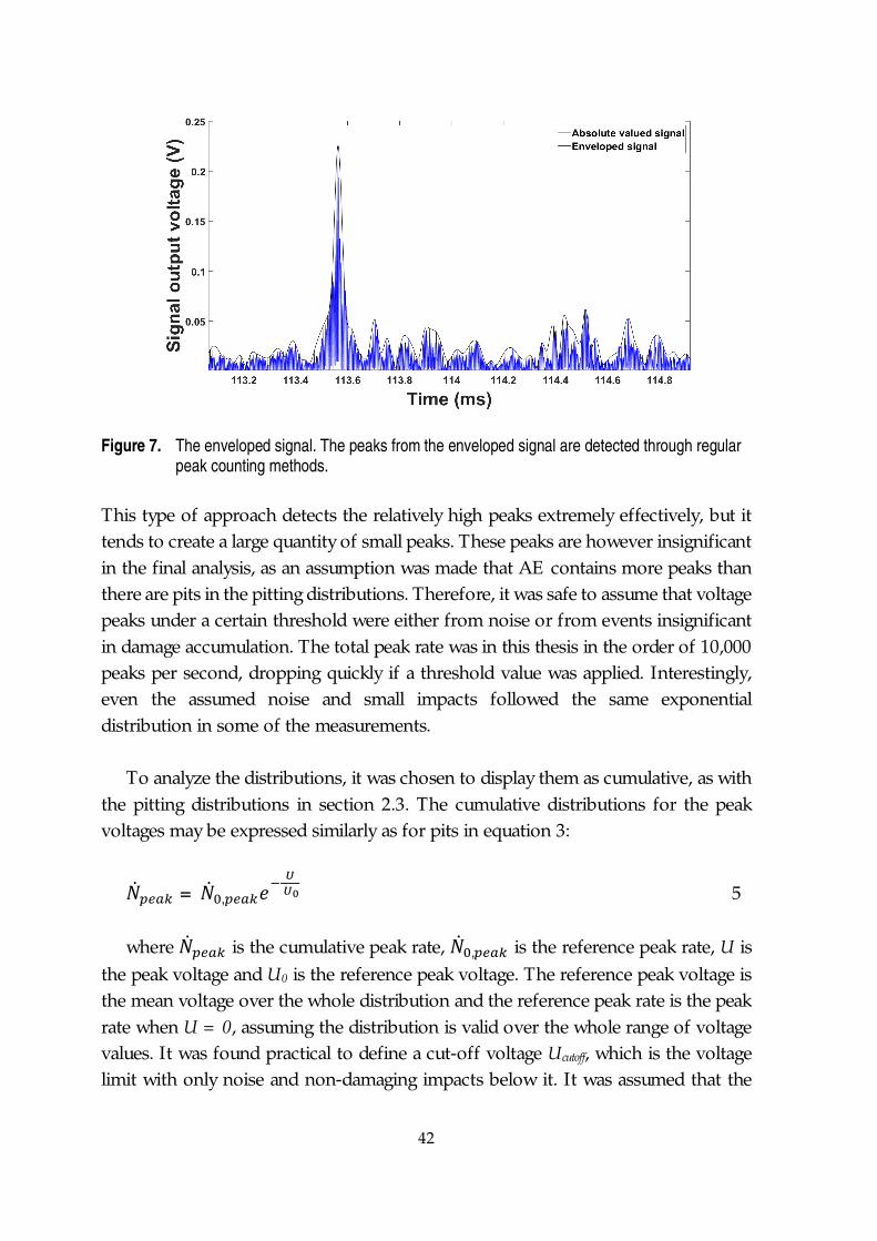
Figure 7. The enveloped signal. The peaks from the enveloped signal are detectedthrough regular peak counting methods. ................................................................. 42

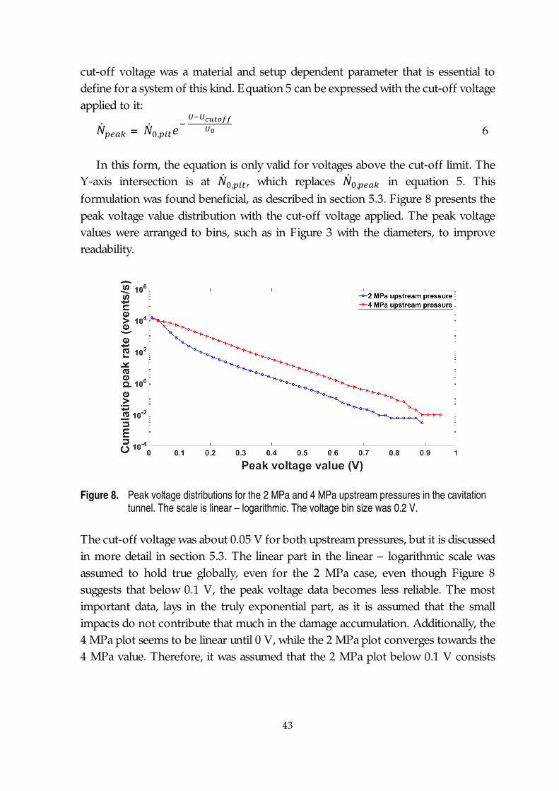
Figure 8. Peak voltage distributions for the 2 MPa and 4 MPa upstream pressuresin the cavitation tunnel. The scale is linear – logarithmic. The voltagebin size was 0.2 V. ....................................................................................................... 43

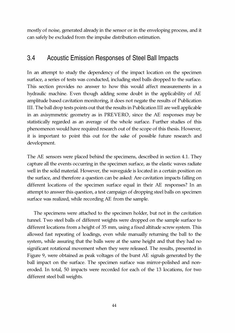
Figure 9. AE peak voltages resulting from steel ball impacts. The maximumvoltage is highly dependent of the impact location in respect to thesensor location. ............................................................................................................ 44

Figure 10. Resonance type sensor, amplitude and average signal level as a functionof erosion time. ............................................................................................................ 46

Figure 11. Resonance type sensor, signal energy and RMS level as a function oferosion time. ................................................................................................................ 47

xiii

Figure 12. Broadband sensor, amplitude and average signal level as a function oferosion time. ................................................................................................................ 47

Figure 13. Broadband sensor, signal energy and RMS level as a function of erosiontime. .............................................................................................................................. 48

Figure 14. The envelope visualization of the high frequency signal acting as acarrier wave to the shedding frequency. The discrete-time analytic signalfollows the original signal (blue) as an envelope (orange). ..................................... 50

Figure 15. Comparison of the original, the decimated and the demodulated signalspectra. The decimated signal was multiplied by 1000 only forvisualization purposes, and in reality, it would overlap almost perfectlywith the original signal spectrum. All spectra were calculated usingWelch’s method ........................................................................................................... 52

Figure 16. Comparison detail of the original, the decimated and the demodulatedsignal spectra. ............................................................................................................... 52

Figure 17. Two options for the waveguide setup. A) The failed LNWDI sensorand B) the one used in most tests, with a regular size sensor fixed insidethe waveguide, and another similar sensor outside the casing. ............................. 57

Figure 18. The contact profilometer measuring a specimen profile. The stainlesssteel specimen is in the left and the profilometer measures the radialprofile. ........................................................................................................................... 59

Figure 19. Comparison of the three different microscopy methods: A) Opticalmicroscopy, 200 X magnification, B) SEM with EBSD mapping of theprior austenite orientations, 500 X magnification, and C) SEM imagewith a 500 X magnification of the eroded surface. ................................................. 62

Figure 20. Average erosion patterns of three different steels. The exposure timeswere 25 hours for the low-alloy steel and 65 hours for both stainlesssteels. The erosion depth divided by eroded cross-section areahighlights the differences in erosion shape. ............................................................. 64

Figure 21. Volume loss dependency on azimuthal angle. The azimuthal angle isexplained in section 2.4. ............................................................................................. 65

Figure 22. Crack propagation in low-cycle fatigue. ................................................................... 68

Figure 23. Pit and peak cumulative distributions. The normalization causes thecurves to overlap to a high degree. The pit diameters and peak voltage

xiv

values were arranged into bins, with the same bin sizes as in Figure 3and Figure 8. ................................................................................................................ 70

Figure 24. Simulated peak (A) and pit (B) distributions for several cavitationtunnel upstream pressures. The scale is linear – logarithmic. ............................... 72

Figure 25. Shedding frequency as a function of eroded volume. ............................................ 74

List of Tables

Table 1. Final volume loss values for the erosion tests as a function of theazimuthal angle. The angle represents the measurement directionin relation to the one defined to be at 0° angle. .......................................... 66

Table 2. Erosion rate dependency on specimen azimuthal angle. The anglerepresents the measurement direction in relation to the onedefined to be at 0° angle. ................................................................................ 67

Table 3. Reference values and simulated distribution values for the connectionbetween peak voltage values and pit diameters. .......................................... 71

xv

ABBREVIATIONS

Greek symbolsρw Density of water

σ Cavitation numberτ Coverage time

Latin symbols( ) Eroded profile area at time tn

( ) Eroded profile area loss at time tn

D0 Reference pit diameter

D Cavitation pit diameter

D0 Reference pit diameterfs Cavitation cloud shedding frequency

H Length parameter in the Strouhal numberℎ ( , ) Eroded profile height at radius r and at time tn

k i A group of geometry parameters in a flow channel

N Amount of samples in an AE signalm Running sample index in a time – analytic signal , AE reference peak rate AE cumulative peak rate , Reference pitting rate Cumulative pitting rate

pd Cavitation tunnel downstream pressure

pr Reference pressure in a hydro machinepu Cavitation tunnel upstream pressure

pv(T) Saturated vapor pressure at temperature T

∆p Pressure difference over a hydraulic systemRe Reynolds number

sr Profilometer radial resolution

St Strouhal number

xvi

T Temperature

t TimeU AE peak voltage value

U0 AE reference voltage

Ucutoff AE cut-off voltageUref AE system reference voltage

V Flow velocity

V c Cavity velocity( ) Eroded profile volume at time tn

( ) Eroded profile volume loss at time tn

X(m) Discrete – time Fourier transform of an AE signal

z(m) One sided N-point discrete – time analytic signal

Abbreviations

AE Acoustic emission

ASL Average signal level

CCD Charge-coupled deviceDTFT Discrete – time Fourier transform

EBSD Electron backscatter diffraction

FEM Finite element methodFFT Fast Fourier transform

HDT Hit definition time

IFFT Inverse fast Fourier transformPVDF Polyvinylidene difluoride

Q&P Quenching and partitioning

RMS Root mean square value

SEM Scanning electron microscopyUHMWPE Ultra-high molecular weight polyethylene

xvii

ORIGINAL PUBLICATIONS

Publication I Ylönen, M., Saarenrinne, P., Miettinen, J., Franc, J-P. & Fivel, M.,2018. Cavitation Bubble Collapse Monitoring by Acoustic Emissionin Laboratory Testing. Proceedings of the 10th Symposium onCavitation (CAV2018): May 14-16, 2018, Baltimore, Maryland, USA.Katz, J. (ed.). ASME, p. 179-184. 05037

Publication II Ylönen, M., Saarenrinne, P., Miettinen, J., Franc, J-P., Fivel, M. &Nyyssönen, T., 2018. Cavitation Erosion Resistance Assessment andComparison of Three Francis Turbine Runner Materials. MaterialsPerformance and Characterization. Volume 7, Issue 5, p. 1107-1126.

Publication III Ylönen, M., Saarenrinne, P., Miettinen, J., Franc, J-P., Fivel, M. &Laakso, J., 2019. Estimation of Cavitation Pit Distributions byAcoustic Emission. Journal of Hydraulic Engineering. Volume 146,Issue 2, p. 1-11.

Publication IV Ylönen, M., Saarenrinne, P., Miettinen, J., Franc, J-P & Fivel, M.,2019. Shedding Frequency in Erosion Evolution Tracking.International Journal of Multiphase Flow. Volume 118, p. 141-149.

Publication V Ylönen, M., Nyyssönen, T., Honkanen, M., Peura, P., UnpublishedManuscript.

xviii

AUTHORS’ CONTRIBUTION

Publication I The author carried out the cavitation and acoustic emission tests anddeveloped the peak counting and enveloping method, with the helpof the other authors. The author prepared the manuscript with thehelp of the others and presented the work in the 10th Symposium onCavitation (CAV2018)

Publication II The author carried out the cavitation erosion tests and developedthe method for calculating volume loss. The SEM images werecaptured in the SIMaP laboratory by a technician, and the authorand Marc Fivel analyzed them. The author prepared the manuscriptwith the help of the others.

Publication III The author carried out the cavitation pitting tests, combined with theacoustic emission measurements. The author and Jean-Pierre Francdeveloped the mathematical formulation for the connectionbetween cavitation pit diameters and peak voltage values of theacoustic emission signal. Jarmo Laakso measured the pitted surfaceusing an optical profilometer. The author prepared the manuscriptwith the help of the others.

Publication IV The author carried out the cavitation erosion tests combined withthe acoustic emission measurements. Jouni Elfvengren proposed theAE signal demodulation process, and it was further developed tosuit the needs of this study by the author. The video recordings werea courtesy of Fabio Villa, who had recorded them earlier. The videosand the AE signals were analysed by the author. The author preparedthe manuscript with the help of the others.

Publication V The author carried out the cavitation erosion tests and analysed thecavitation-related part of the manuscript. Mari Honkanen performedthe EBSD measurements and Tuomo Nyyssönen analysed themicrostructures of the steels and drew the conclusions regarding thereasons behind cavitation erosion resistance for the martensiticstainless steels. The manuscript was prepared equally by the author,Tuomo Nyyssönen and Mari Honkanen, and it was widelycommented by Pasi Peura.

19

1 INTRODUCTION

1.1 Background

Cavitation is a major source of damage and vibrations in many modern hydromachines. Cavitation occurs when the static pressure of a liquid drops below acertain threshold, leading to the evaporation of the liquid. Typically, this thresholdis the saturated vapor pressure of the liquid. It may also be lower, if there are nonucleation sites for the evaporation to commence. When cavitation occurs in a liquidflow, in a low static pressure region, there is a chance that the vapor bubbles travelto a higher-pressure region and violently collapse. If these collapses occur near asolid boundary, material damage may occur. This damage is called cavitation erosion.Typically, monitoring cavitation and cavitation erosion during machine operation isdifficult, or even impossible. (Brennen 1995; Franc & Michel 2005)

This thesis addresses the issue of cavitation monitoring by presenting novelmethods related to acoustic emission (AE) measurement. The aim is to monitor onlydamaging cavitation: Damage in the form of individual pits or damage in the formof cumulating material loss. AE measurement differs from acoustic soundmeasurement, as AE refers to elastic waves traveling in a solid, rather than wavestraveling in a fluid. The source of these elastic waves can be internal stresses in amaterial, external impacts, or surface contacts leading to energy release in thematerial structure. Their expected frequency range is typically from 100 kHz to 1MHz. Typically, they have a wide frequency band, as the elastic waves are the resultof events intrinsically of wide frequency range. (Holroyd 2000; Grosse 2008).

The current work concentrates on laboratory measurements, performed at theLEGI laboratory, using a high-speed cavitation tunnel (PREVERO 2018). Thelaboratory measurements provided an environment where the primary AE sourcewas cavitation, while all other sources were irrelevant in magnitude. In a hydraulicmachine environment, other sources such as rolling bearings or flow related impactsmight distract the measurements. In a laboratory environment, there was no doubt

20

that the AE signal source was cavitation, and more importantly, that the damage tothe specimens was due to cavitation impacts. AE does not properly detect cavitationevents that occur far from surfaces, as the directed impacts towards walls lead tosignificantly higher AE responses (van Rijsbergen et al. 2012). For this reason, thepotentially damaging events are detected, while the non-damaging events occurringin the free fluid are excluded. With this approach, the AE response of erosive andnon-erosive cavitation was identified, thus providing a baseline for the extension toa hydraulic machine, in possible future applications.

To study the possibilities of AE in cavitation monitoring, two approaches werechosen: Cavitation pitting tests to detect individual impacts and their magnitudes,and cavitation erosion tests to study if AE could reveal parameters that change whenthe material erodes further. In the pitting tests, the cavitation collapses affected alimited area on the specimen, leading to elastic and plastic deformation and pits withno significant overlapping. It was expected that the impact strength would beconnected to the AE response magnitude. These pitting tests had a short duration,typically a few minutes, while the erosion tests had a duration of tens of hours. Inthe erosion testing, individual impacts were not detected, as the damage overlappingbegins to change the material and therefore AE responses so that it was not possibleto characterize the impacts. It was expected that parameters would be found thatchange during the erosion tests, as the surface geometry changes and the materialstrain-hardens significantly; therefore, affecting the bubble – surface interaction, andpossibly the resulting AE signal.

1.2 Objectives and Scientific Contribution

The main research objectives and research questions of this thesis were:

1. How fast do the studied steels, used in Francis turbine runner blades, erodein a cavitation tunnel?

2. What are the main reasons behind the differing cavitation erosion rates?

3. Can individual, damaging cavitation impacts be detected and characterizedvia acoustic emission?

21

4. Can acoustic emission be used in tracking the erosion process of a materialexperiencing cavitation erosion?

The main approach was to study the material specimens in a cavitation tunnel,combined with AE measurements. A vast campaign of experiments was carried out,with no prior knowledge if the research questions could be answered. Three differentmaterials, specimens from runner blades of Francis turbines, were subjected tocavitation both in pitting tests and in erosion tests. The pitting tests were expectedto provide information about individual cavitation impacts and about the impactload distributions. The aim of the erosion tests was to seek knowledge about erosionrates, and more importantly, to find if acoustic emission could be used in trackingthe erosion evolution. The main scientific contributions of this thesis were:

1. characterizing the cavitation erosion rates of the turbine steels andidentifying the main erosion mechanisms and the reasons behind thediffering erosion resistances (Publications II and V);

2. linking the cavitation pit diameter distributions to the acoustic emissionpeak voltage distributions, thus creating a method to characterize acavitation field in terms of resulting pit diameters, regardless of cavitationintensity (Publications I and III); and

3. proposing a method to identify the cavitation cloud shedding frequencyby acoustic emission, and finding a way to track erosion evolutionthrough the changes in this frequency (Publication IV).

The author’s initial work with cavitation begun in (Ylönen 2016). In this master’sthesis, one of the steel specimens was eroded, while recording AE with a setupinferior in performance to that used in later work. This initial work allowed theauthor to acquire the basic skills to properly run the cavitation tunnel and performthe erosion tests. The gained knowledge was also used in defining the requiredperformance of the new AE setup.

The pitting tests are a well established method in cavitation research. However,combining these tests with AE and counting the AE peak voltages was a novelapproach. Publication I explains how the AE peak voltages were extracted fromenveloped AE signals, and how they were distributed, depending on the cavitationintensity. Publication III utilizes this method in combining pit distributions and AE

22

peak distributions, thus finding a way to estimate the cavitation intensity in thecavitation tunnel without access to the pitted surface of the specimens.

During all the erosion tests, AE was measured along with the volume loss processof the specimens. Publication II studies the erosion rates of all the three studiedmaterials, the erosion process, and the reasons behind the differing rates. The AEpart of the erosion studies is discussed in Publication IV, where the tracking of thecavitation cloud shedding frequency was introduced, in order to first identify thisfrequency, and then use it in erosion evolution tracking. Publication V concentrateson the differences in microstructure between two of the studied steels, the mainfinding being that residual austenite seems to reinforce martensitic stainless steelsagainst cavitation impacts.

23

2 CAVITATION AND CAVITATION EROSION

2.1 Cavitation

According to (Arndt 2014) Froude was the first to use the term cavitation, probablyin 1895. Euler was first to study and problematize cavitation, without using the term,in his 1754 memoir and Reynolds was the first to carry out a study about cavitationin a constricted tube. Cavitation was for the first time found problematic in shippropellers, as their rotation speed begun to exceed the critical values for cavitationto occur. Rayleigh was the first to calculate, in 1917, the erosion potential of anindividual bubble. Obviously, the early models were simplified, and insufficient inproperly assessing the complex process of, for example, bubble cloud formation,cavitation inception, collective bubble collapses and material resistance and responseto cavitation impacts. Cavitation remains an important topic, as modern hydraulicmachines tend to be operated at their maximum performance and utility, often inthe vicinity of damaging cavitation.

The basic knowledge and understanding of cavitation and cavitation erosion isbest found from several textbooks. Young’s book Cavitation (Young 1989) offers a lotof knowledge on the basic principles behind the phenomenon. Brennen’s Cavitation

and Bubble Dynamics (Brennen 1995) and Franc and Michel’s Fundamentals of Cavitation

(Franc & Michel 2005) both present all the required basic knowledge and they offersupplemental information about some of the more advanced features. Kim et al.wrote the A dvanced E xperimental and Numerical Techniques for Cavitation E rosion Prediction

(K. H. Kim et al. 2014). It concentrates more on the advanced features of cavitation,most notably cavitation erosion. Half of it is studies and conclusions presented bythe authors and half of it is selected papers from the most recent and advancedstudies of cavitation erosion. All these were important sources for this thesis.

Cavitation may occur in a static or a moving liquid, although cavitation in a liquidflow is more representative of the case of hydro machines. The drop in pressureleads to the breakdown of the bonds between molecules that compose a liquid, i.e.it vaporizes. The vapor-liquid equilibrium pressure is the saturated vapor pressure.

24

For water, it is 2315 Pa at 293 K temperature (Mills 1999). However, the nucleationof vapor bubbles require nucleation sites, such as non-condensed gas or otherimpurities. In absence of these nucleation sites, a static liquid may experience ametastable state at negative absolute pressure, called tension (Berthelot 1849-1858;Caupin & Herbert 2006; Heyes 2008). In the case of hydraulic machines, nucleationsites are often abundant. Therefore, it is often practical to consider the criticalpressure for cavitation to be the saturated vapor pressure.

Rayleigh (Rayleigh 1917) first mathematically described the growth – collapsecycle of a spherical bubble in an infinite liquid. Plesset (Plesset 1949) improved theformulation, and thus found further insights regarding the life of a cavitation bubble(Plesset 1970; Plesset & Chapman 1971; Plesset & Prosperetti 1977). Several authorscontinued the mathematical formulation of the process, thus generating fundamentalknowledge about the lifetimes and sizes of idealized bubbles (Knapp et al. 1970);Acosta & Parkin 1975; Hammitt 1979). These mathematical formulations are thebasis of cavitation research and they offer guidelines of what to expect from bubbles;therefore, they are worth mentioning. This thesis, however, concentrates onempirical studies, and these equations were never used.

The collapse process of a cavitation bubble in free liquid is symmetrical: Thevapor bubble collapses towards its center, and finally it generates a shock wave, whenthe bubble walls collide. The driving force is the pressure difference: Inside thebubble the pressure is initially saturated vapor pressure, while outside the pressure isthe ambient liquid pressure. The more interesting case is the bubble collapse near aboundary. Due to an asymmetrical pressure field, the bubble wall away from theboundary begins to collapse first. This leads to a liquid jet traversing the bubble anddirected to the boundary. The liquid jet gains a significant velocity, and hits theboundary, potentially causing damage. In addition to that, the formed bubble ringcollapses violently, also potentially causing damage. (Zhang et al. 1993; Zhang et al.1994; Brujan et al. 2002; Obreschkow 2012)

An essential parameter in many cavitation studies is the cavitation number. Thecavitation number is a non-dimensional parameter that is essentially the ratiobetween the difference of a reference pressure in a hydraulic system and saturatedvapor pressure, and the pressure difference over the system. It is useful in definingthe inception or closure of cavitation in the system, as they typically occur at thesame cavitation number regardless of pressure level. Additionally, cavitation in a

25

system tends to have same characteristics, such as the closure location of cavitation,with the same cavitation number but different overall pressure or flow velocity. Thepressure difference is related to the flow velocity of the system; therefore, the ratiois between static pressure and dynamic pressure. The cavitation number σ is generallydefined as (Franc & Michel 2005):

=( )Δ 1

where pr is the reference pressure, pv(T) is the saturated vapor pressure at the flowtemperature and ∆p is the pressure difference over the system. The referencepressure is typically a pressure conveniently measurable, such us the downstreampressure of the system. The cavitation number is a relative parameter, so the exactvalue alone gives no insight if there is cavitation in the system or not. The cavitationtunnel used in this study has its cavitation inception at σ ≈ 2.8, and the erosion testswere done at σ ≈ 0.87, where cavitation may be considered fully developed.

This thesis concentrates in experiments carried out in a hydrodynamic cavitationtunnel (PREVERO 2018). The tunnel produces a cavitation type typical tohydrofoils: The cloud cavitation. Traveling bubbles, which is the first main type ofcavitation, may form in a low-pressure region and then travel to a higher-pressureregion and disappear either by collapsing or by slow reduction of size. Thesetransient isolated bubbles are usually less erosive than attached or sheet cavities,which are the second main cavitation type. The attached cavities form in the leadingedges of hydrofoils or blades. They follow the flow towards the trailing edge, andpotentially collapse near the foil surface, thus promoting damage. An oscillatingsheet cavity is called a cloud cavity, discussed in more detail in section 2.2. The lastmain type of cavitation are the cavitating vortices. A vortex core has a lower pressurethan the rest of the vortex. With high enough vorticity, the core may cavitate. Thesecavitating vortices may for example form between turbine blades, if the water flowangle of attack is not optimal. It has the potential to be highly damaging. (Avellan2004; Franc & Michel 2005; Escaler et al. 2006).

2.2 Cloud Cavitation Shedding Frequency

Cloud cavitation is characterized by an oscillating growth-collapse cycle of a groupof cavitation bubbles. This cloud typically grows attached to a surface, until it reaches

26

a critical length for a liquid counter-current flow to form between the cavity and thesurface. This counter-current flow detaches the cloud from the surface, leading tothe near-simultaneous collapse of all the bubbles in the cloud. The bubble collapsestend to initiate further collapses, thus the collapse of the cloud is self-driven, after ithas begun. If the collapse occurs sufficiently near to the surface, damage may occur.The main parameters affecting the formation of such clouds are the flow velocity,overall pressure, liquid quality, flow geometry and surface quality. By increasing flowvelocity around a hydrofoil, starting from no-cavitation state, cavitation typicallybegins as individual bubbles, followed by a sheet cavity with no periodical cloudformation. With more velocity, a cloud pattern begins to appear, and with asufficiently high velocity, super cavitation occurs, where cavitation closure is outsidethe hydrofoil. (Brennen et al. 2000; Franc & Michel 2005; Nishimura et al. 2014;Gnanaskandan & Mahesh 2016; Hsiao et al. 2017)

The transition from sheet to cloud cavitation occurs at a critical cavitationnumber. The cavitation number for cavitation inception is the number where theinitial individual bubbles begin to form. The inception of cavitation may be pinnedto quite an exact cavitation number, but the transition from sheet to cloud cavitationincludes a transient area. Additionally, the cavitation number for the transition is alsodependent of the flow Reynolds number. (Pelz et al. 2017) mapped the transition intheir testing geometry that was a converging-diverging nozzle. With a low Reynoldsnumber, the cavitation remains a sheet even with low cavitation numbers, andincreasing the Reynolds number increases the critical cavitation number. A narrowtransition region is found between the sheet and cloud cavitation regions. (Keil et al.2012)

The frequency of the cloud formation and collapse cycle is dependent of theReynolds number, cavitation number and channel geometry. Typically, the frequencyis expressed through the Strouhal number, which is a dimensionless number definedas (Pelz et al. 2014):( , , ) = 2

where Re is the Reynolds number, k i is the group of geometry parameters, forexample related to channel curvature, fs is the shedding frequency, H is the lengthparameter, for example channel height, and V is the flow velocity. Above a critical

27

Reynolds number, the Strouhal number is no longer dependent on the Reynoldsnumber, only on the cavitation number and channel geometry (Pelz et al. 2014).

The geometry parameter could include the surface roughness of a channel. Thisnotion is interesting in the scope of this thesis, as an increase in roughness wouldcorrespond to increased cumulative erosion, as explained in Publication IV. This issupported by the observations of (Hao et al. 2017), who found a shedding frequencyof 17 Hz for a smooth hydrofoil, while that of a rough hydrofoil was 20 Hz, in equalflow conditions. (Stutz 2003) found no influence of roughness to the sheet cavityshape, void fraction or time-averaged velocity. This suggests that the roughnessinfluences the circulation of the counter-current flow between the cloud cavity andthe surface, but not the cavity itself.

One of the main goals in this thesis was to monitor the evolution of cavitationerosion. Monitoring this shedding frequency proved to be the most reliable way, asthe frequency was consistently found using acoustic emission measurements. Theshedding frequency is not particularly difficult to find in general, via for examplevideo analysis, but measuring it by AE provides a way to define the frequency duringoperation and without visual access to the flow. A pressure sensor in the channelwall sufficed for (Keil et al. 2012) and (Pelz et al. 2014), but AE has the advantagethat it is installed outside the flow, to a solid surface that has a solid transfer path tothe cavitating region. However, correlating the shedding frequency changes toerosion evolution was a novel approach, as far as the author of this thesis is awareof, and it was first presented in Publication IV.

The most reliable way to study the cloud cavitation phenomenon in a laboratoryenvironment is filming it with a high-speed video camera. This approach was alsoused for Publication IV, to verify that the frequencies defined through AE are thecorrect ones. The videos were kindly provided by (Gavaises et al. 2015), who alsohad analyzed them. They were reanalyzed for Publication IV with a slightly differentapproach. The simulation results for the cavitation tunnel geometry by (Gavaises etal. 2015) were also compared to the frequencies defined by AE and the videoanalysis, and all three were consistent with each other.

The high-speed videos from cavitation were recorded so that the cloud length iswell captured. They were filmed only from one direction, so no accurate imaging ofthe cloud structures was available. The experimental procedure is explained in more

28

detail in (Gavaises et al. 2015). The 2-D image was sufficient for finding the mainfrequencies associated to the cavitation, as long as there was a cloud structure.Several overall pressures and cavitation numbers were included, with cavitationnumbers where assumedly the structure was sheet cavitation rather than cloudcavitation.

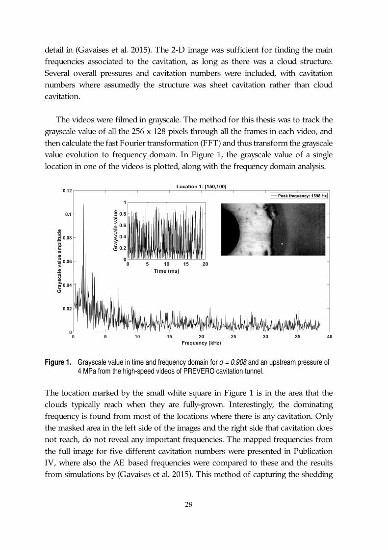
The videos were filmed in grayscale. The method for this thesis was to track thegrayscale value of all the 256 x 128 pixels through all the frames in each video, andthen calculate the fast Fourier transformation (FFT) and thus transform the grayscalevalue evolution to frequency domain. In Figure 1, the grayscale value of a singlelocation in one of the videos is plotted, along with the frequency domain analysis.

Figure 1. Grayscale value in time and frequency domain for σ = 0.908 and an upstream pressure of4 MPa from the high-speed videos of PREVERO cavitation tunnel.

The location marked by the small white square in Figure 1 is in the area that theclouds typically reach when they are fully-grown. Interestingly, the dominatingfrequency is found from most of the locations where there is any cavitation. Onlythe masked area in the left side of the images and the right side that cavitation doesnot reach, do not reveal any important frequencies. The mapped frequencies fromthe full image for five different cavitation numbers were presented in PublicationIV, where also the AE based frequencies were compared to these and the resultsfrom simulations by (Gavaises et al. 2015). This method of capturing the shedding

29

frequencies by video analysis proved to be a simple, effective and fast method todecipher if there is an oscillating cloud cavity in the system, at least in the limitedscope of the laboratory tests in the tunnel. Probably, in a more complex geometry,the cloud cavitation phenomenon would have to be filmed with stereoscopic imagingto capture the periodicity properly.

2.3 Cavitation Pitting

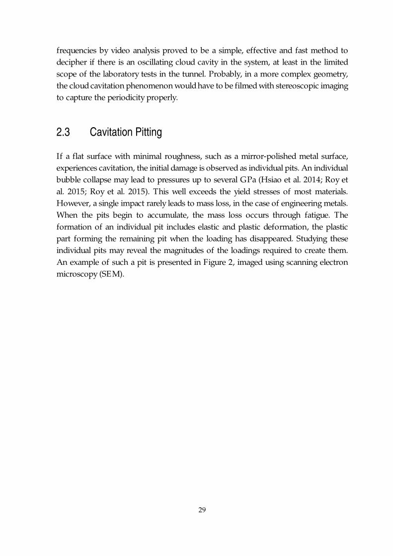
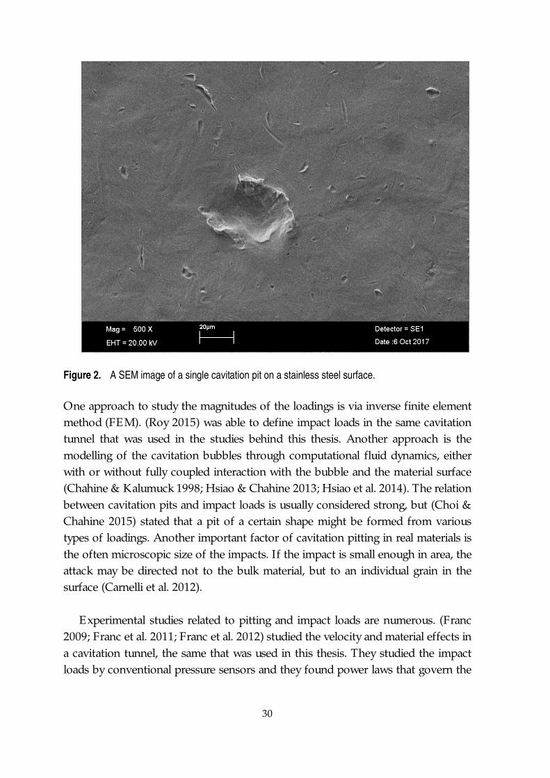
If a flat surface with minimal roughness, such as a mirror-polished metal surface,experiences cavitation, the initial damage is observed as individual pits. An individualbubble collapse may lead to pressures up to several GPa (Hsiao et al. 2014; Roy etal. 2015; Roy et al. 2015). This well exceeds the yield stresses of most materials.However, a single impact rarely leads to mass loss, in the case of engineering metals.When the pits begin to accumulate, the mass loss occurs through fatigue. Theformation of an individual pit includes elastic and plastic deformation, the plasticpart forming the remaining pit when the loading has disappeared. Studying theseindividual pits may reveal the magnitudes of the loadings required to create them.An example of such a pit is presented in Figure 2, imaged using scanning electronmicroscopy (SEM).

30

Figure 2. A SEM image of a single cavitation pit on a stainless steel surface.

One approach to study the magnitudes of the loadings is via inverse finite elementmethod (FEM). (Roy 2015) was able to define impact loads in the same cavitationtunnel that was used in the studies behind this thesis. Another approach is themodelling of the cavitation bubbles through computational fluid dynamics, eitherwith or without fully coupled interaction with the bubble and the material surface(Chahine & Kalumuck 1998; Hsiao & Chahine 2013; Hsiao et al. 2014). The relationbetween cavitation pits and impact loads is usually considered strong, but (Choi &Chahine 2015) stated that a pit of a certain shape might be formed from varioustypes of loadings. Another important factor of cavitation pitting in real materials isthe often microscopic size of the impacts. If the impact is small enough in area, theattack may be directed not to the bulk material, but to an individual grain in thesurface (Carnelli et al. 2012).

Experimental studies related to pitting and impact loads are numerous. (Franc2009; Franc et al. 2011; Franc et al. 2012) studied the velocity and material effects ina cavitation tunnel, the same that was used in this thesis. They studied the impactloads by conventional pressure sensors and they found power laws that govern the

31

pit distributions, with normalized flow velocities. A different approach was by (Hujeret al. 2015; Hujer & Muller 2018), who fitted specimens with polyvinylidenedifluoride (PVDF) pressure sensors. Additionally, (Carrat et al. 2017) utilized thesame sensors to study the impacts on a hydrofoil experiencing cavitation. The PVDFsensors are well suited for defining the actual impulse pressures in a cavitation test(Kang et al. 2018). A common factor in the studies in this particular cavitation tunnel,regardless of methods, was that the pit and impact distributions followed anexponential law: The larger the pit diameter or the impact strength, less numerousthey are in a statistical analysis.

The fact that the expected distribution is exponential was helpful in determiningfirstly if measurements were likely to be correct. In the AE measurements especially,there were occasions that the measured distributions were far from exponential.Further analysis showed problems such as signal saturation or sensor malfunction.The exponential distribution of pits can be well expressed as a mathematical formula,and its properties may be easily compared, especially when a similar distribution isfound from pressure or AE measurements. The distributions were found to be morepractical to present as cumulative distributions. An exponential cumulativedistribution in cavitation pitting is expressed as:

= , 3

where is the cumulative pitting rate, , is the reference pitting rate, D isthe pit diameter and D0 is the reference pit diameter. The diameter was defined asthe equivalent diameter of a circle, calculated from the pit surface area. The referencepit diameter D0 is the mean value of pit diameters over the distribution. The referencepitting rate , is the pitting rate when = 0. It is possible to quantify the pitsize accurately for a single pit. However, for a pit distribution to be statistically valid,one needs to measure at least hundreds of pits. This leads to practical limitations inthe measurement setup. In Publication III, the pits were detected using an opticalprofilometer with a 3.5226 μm x 3.5226 μm measurement grid. The grid resolutionwas a compromise between accuracy and measurable surface size. With thisresolution, the minimum observable pit diameter was 15 μm, but the completeeroded surface could be analyzed. This minimum pit diameter effectively leads to theignoring of smaller pits, as observed in Figure 3. The diameters were sorted into binsand afterwards sorted according to their sizes. This makes the figures clearer, as eachbin may contain tens to hundreds of measured diameters.

32

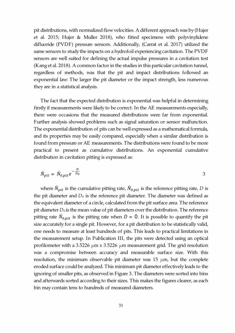
Figure 3. Cumulative pitting rate as a function of pit diameter for 2 MPa and 4 MPa upstreampressures. There are no detected pits below the 15 μm limit, observed as flattening of thelinear curves. The diameter bin size was 1 μm. The scale is linear – logarithmic.

The ignored small pits of diameter less than 15 μm are observed as a flat part in themeasured curve. It does not mean that they would not exist in the eroded surface.An assumption was made that the exponential distribution follows equation 3globally. This assumption is based on the measurements by (Franc et al. 2012), whomeasured the same types of samples using a different profilometer. They had a betterresolution with a smaller measured surface, and they found pits of the size of a fewμm, still following the exponential distribution. The linear part of the plot in Figure3, which is in linear – logarithmic scale, corresponds to an exponential distribution.According to this assumption, the linear trend continues below the profilometer-based limit of about 15 μm. The 2 MPa and 4 MPa upstream pressures correlate withthe cavitation velocity, overall cavitation tunnel pressure and cavitation intensity, asfurther explained in section 4.1.

2.4 Cavitation Erosion

The evolution of cavitation erosion in metals may be divided into three or fourstages, depending on the case: 1) The incubation period, 2) the acceleration period,3) the steady state period and 4) the deceleration. The incubation period is the periodwhere a virgin material starts to experience cavitation erosion and the impacts causemostly plastic deformation in the form of pits, such as presented in section 2.3. As

33

the pits begin to overlap, cracking and rupture starts to occur and the erosion movesthrough acceleration period to steady state period, where the material loss rate isrelatively constant. In the deceleration period, the material surface is filled withstructural cavities that begin to damp the incoming cavitation impacts, thus reducingmaterial loss rate. In cavitation testing, the deceleration period is not always reacheddue to limitations in the testing procedures. (Zhou & Hammitt 1983; Berchiche etal. 2002; Franc 2009; Franc et al. 2014; Chahine et al. 2014)

Cavitation erosion often cumulates slowly in hydraulic machines, as strongcavitation is normally detected as machine vibration, noise and performance drop.Therefore, these operating conditions are naturally avoided. However, slowlycumulating erosion processes lead to a loss of structural integrity, loweredperformance and in the worst case, in machine breakdown, if they are not assessedproperly. Cavitation and cavitation erosion may be avoided by machine design, butit is not desirable to design machines too safely out of range for cavitation to happen,due to lowered performance. Therefore, somehow knowing the extent of erosion inlong-term operation is important. (Arndt et al. 1989; Farhat & Bourdon 1998;Bourdon et al. 1999)

In designing machines that can endure cavitation, material resistance to cavitationerosion is an important parameter. The resistance to cavitation is often closely linkedto the material strength in terms of typical mechanical parameters, as in studies by(Hammitt 1979; Zhou & Hammitt 1983; Hattori & Nakao 2002; Hattori et al. 2004;Hattori & Ishikura 2010). This is not always true, as cavitation impacts may erode anarea smaller than the material grain size, thus attacking also the softer grains in anisolated manner. For this reason, the macro-scale parameters might not provideinformation about the strength against cavitation. Additionally, the impacts have ahigh strain rate of up to 106 1/s (Karimi & Leo 1987). This means that the strain ratedependency of the material has an important role. Additionally, the erosive potentialof cavitation depends on the cavitation type. (Carnelli et al. 2012; Roy 2015)

Considering all these factors, the resistance to cavitation may be stated as case-dependent, and there is no single exact parameter to define the goodness of amaterial in hydraulic channels potentially experiencing cavitation, even thoughstronger material usually means better resistance. There are multiple cavitationtesting methods to compare materials. The test methods differ in how they generatecavitation and in which form. Some of these testing methods are listed here:

34

· The (ASTM G32-10, Standard Test Method for Cavitation Erosion UsingVibratory Apparatus 2010) is a vibrating horn for basic and relatively lowcost cavitation testing. The material specimens are attached to a vibratinghorn that is in a static liquid. Cavitation is created as the pressure field aroundthe specimen oscillates, thus creating tension in the liquid. This type oftesting was done for example by (Kendrick et al. 2005; Hattori & Kitagawa2010; Hattori et al. 2010; He & Shen 2012; Pöhl et al. 2015).

· The (ASTM G134-95(2010)e1, Standard Test Method for Erosion of SolidMaterials by a Cavitating Liquid Jet 2010) is a system that directs a liquid jeton a specimen resting in static liquid. Cavitation is created in the shear layerbetween the moving jet and the static liquid. It was used for example by(Soyama & Futakawa 2004; Soyama 2013; Nishimura et al. 2014).

· Different types of rotational setups that are based on periodically openingand closing valves. Cavitation forms due to expansion waves that thismotion creates. Some examples are presented in (Karimi 1987; Auret et al.1993).

· Cavitation tunnels of various types. Cavitation tunnels are utilized both tostudy cavitation structures and cavitation erosion. Cavitation structures werestudied for example by (Steller et al. 2005; Arabnejad et al. 2018; Chen et al.2018) and erosion in a cavitation tunnel by (Dular et al. 2006; Dular &Osterman 2008; Franc et al. 2012).

The ASTM G32 typically involves weighing the specimens. The specimens are small,about 10 mm high and about 10 mm diameter cylinders, and the eroded surfacerepresents a relatively significant amount of the total specimen mass. Therefore, themeasurement resolution is sufficient. However, for example in the tunnel used forthis thesis, weighing the specimens would be impractical. The eroded area does notcover the whole specimen, which is a 20 mm high and 100 mm diameter cylinder.Measuring milligrams of erosion would be difficult from a specimen that weighsmore than 1 kg, if it is steel. For this reason, and also to provide additionalinformation about the erosion profile, measuring surface profiles is a better optioncompared to weighing. Material loss may be simply calculated from the surfaceprofiles.

35

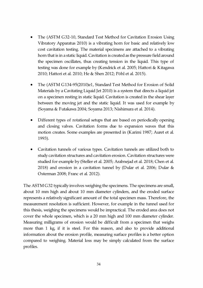
In this thesis, the surface profiles were measured using a contact profilometer.The eroded surface was a circle, with a ring shaped cavitation pattern that has amaximum erosion rate approximately in the radial distance of 22 mm from thespecimen center. The entire eroded area ranges from 19 mm to 32 mm radius, asobserved in Figure 4. Initially the specimen was mirror polished, and it remained sothrough the test campaign outside the area of effect of cavitation.

Figure 4. Eroded stainless steel specimen after 65 hours of cavitation. The arrow indicates theprofile measured for Figure 5.

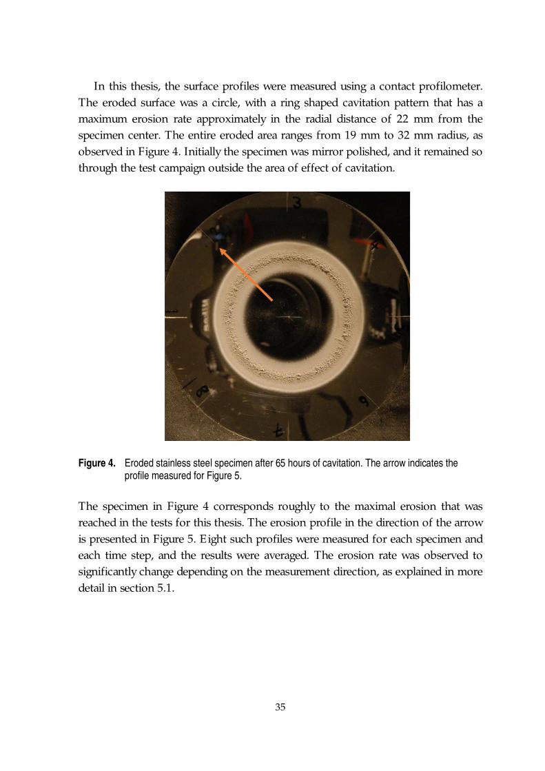
The specimen in Figure 4 corresponds roughly to the maximal erosion that wasreached in the tests for this thesis. The erosion profile in the direction of the arrowis presented in Figure 5. Eight such profiles were measured for each specimen andeach time step, and the results were averaged. The erosion rate was observed tosignificantly change depending on the measurement direction, as explained in moredetail in section 5.1.

36

Figure 5. Surface profile of the eroded stainless steel specimen in Figure 4. The initial profile isvirtually flat, compared to the significantly eroded surface after 65 hours of cavitation atmaximum aggressiveness.

The initial surface profiles were almost flat, compared to the eroded profiles. Thevariation from the zero level due to imperfect polishing in the eroded area wastypically less than one μm. Therefore, in terms of volume loss the initial profile hadno significance when calculating the volume loss of evolved erosion stages. Anyhow,the initial profile was measured and the volume losses of later stages were correctedby subtracting that of the initial stage.

37

3 CAVITATION DETECTION BY ACOUSTICEMISSION MEASUREMENTS

3.1 Acoustic Emission

Acoustic emission is defined as elastic waves that travel in a solid material. The wavesare the result of material internal stresses, external impacts or surface contacts. Theyusually have a wide frequency band, resulting from the wide frequency band of theAE event. Typically, AE is sought from the range of 100 kHz to 1 MHz, but in someapplications, wider ranges may be useful. Piezoelectric sensors are used in measuringAE. They are attached to a surface that has a good transfer path to the expected AEsource. AE measurements could be compared to seismic measurements, as AEsensors measure the surface motion, as do the seismograms, but the scale being inthe micro rather than the macroscale. (Achenbach 1975; Holroyd 2000; Grosse 2008;Ohtsu et al. 2016)

Cavitation is typically considered as noise in AE measurements, as they are oftenused in structural integrity monitoring. That monitoring suffers greatly if there iscavitation near the target AE source, as it tends to bury all other signals underneathit due to its larger magnitude. In this thesis however, cavitation is the targetparameter. Cavitation was found to induce AE voltages of about 100 times largerthan the signal from a flow without cavitation. Therefore, it was practical to assumethat all strong signals were directly or indirectly the result of cavitation.

An AE signal is typically symmetrical around zero volts and the positive andnegative voltages measure the same phenomenon. AE signals may be divided intotwo main categories: burst signals and continuous signals. Continuous AE may befor example the result of friction in a sliding contact, such as in a bearing, and it istypically harder to characterize (Grosse 2008). Burst signals result from shortduration releases of energy, such as in crack propagation, or relevant to this thesis,short duration impacts such as from cavitation bubble collapses. The burst signalsare typically relatively rare, representing only a tiny fraction of the total measurement

38

time. However, in the cavitation tunnel used in this thesis, they were so numerousthat they almost overlapped. Publication III presents these results.

In addition to the categories of burst signals and continuous AE, anotherimportant classification is the sensor types. The two main types are the resonancetype sensor and the broadband sensor. Both of them are in similar casing, typicallya metal cylinder of about 20 mm high and 20 mm diameter, with the detection facemade of a ceramic material. The resonance type sensor has a distinct resonancefrequency that is amplified inside the sensor. The resonance frequency is dependenton the piezoelectric element size and material. The broadband sensor design differsfrom the resonance type only so that it has a damping material around thepiezoelectric element. This damping suppresses wave reflections inside the sensor,thus reducing the resonance frequency amplification and leading to a flatterfrequency response. (Ohtsu 2008; Inaba 2016)

AE is often treated in separate “hits”. A hit is an event of AE activity that beginswith the crossing of a voltage threshold that is either preselected, or tied to thecurrent average signal level. The hit ends, when a preselected time, called the hitdefinition time (HDT), has passed without any threshold crossings. The parametersdefining AE activity are usually calculated over these hits. Typical parameters,according to (Ohtsu et al. 2016), are listed here:

1) AE signal amplitude. The peak amplitude of the hit is the maximum absolutevoltage of the hit, expressed either in volts or in decibels. In decibels, theamplitude is calculated as:( ) = 20 4

where U is the peak voltage value and Uref is the AE system reference voltage,usually 1 μV.

2) AE count expresses the amount of threshold passings in a hit. AE count rateis the AE count divided by hit length.

3) AE energy is either the time integral of the absolute values or the timeintegral of the squares of the absolute values over the hit. The squaredintegral produces values in Joules, if it is divided by an assumed systemimpedance, for example 10 kΩ in many systems.

39

4) Hit duration is the time from trigger to end of hit.

5) Rise time is the time it takes from the trigger to maximum amplitude.

6) Ratio of rise time to amplitude. This parameter provides insight on howshort the event is compared to its amplitude. This may also be expressed interms of counts before peak amplitude.

7) AE root mean square (RMS) value. RMS value is the square root of the meanvalue of the squared voltage values over a hit.

8) Average signal level (ASL). ASL differs from RMS so that the mean value istaken from the absolute values instead of their squared values.

The AE setup calculates these parameters by default, in one form or another, alongwith some other additional parameters. Spectral parameters, such as peak frequency,average frequency or frequency centroid, are often recorded as well. AE setups oftensave the data as parameter groups defining each hit, but they might also be able torecord full waveforms, either for a short period or continuously, depending onhardware capability. These full waveforms allow any imaginable parameters to becalculated in post-treatment, which was found very useful in this thesis.

3.2 Cavitation and Acoustic Emission

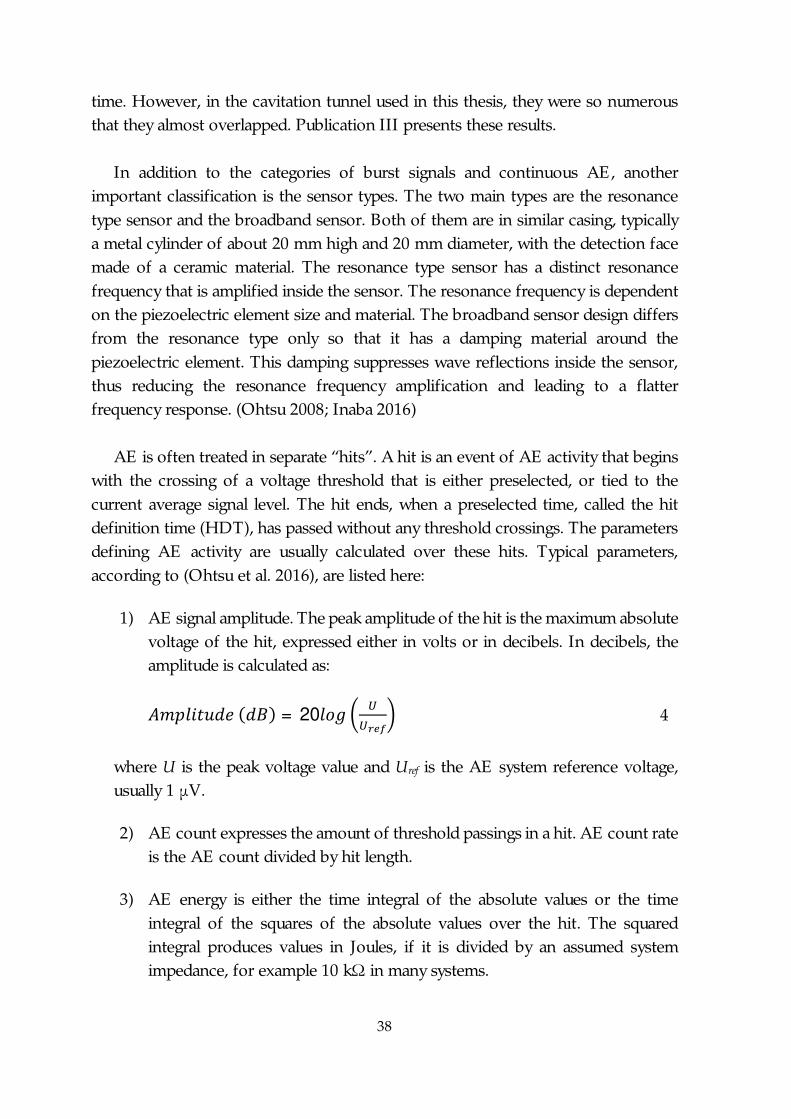
As already mentioned in section 3.1, the cavitation tunnel used in this thesis providedcavitation intense enough for the events to almost overlap in the AE signal. Twosensor types were used in all measurements: One resonance type sensor and onebroadband sensor. The resonance type sensor was found to be more sensitive to theburst signals resulting from the cavitation bubble collapses. This is probably due tothe structure of the sensors. While the damping in the broadband sensor flattens thefrequency response, it also probably increases the rise time of the sensor response.This is well perceived in Figure 6, where broadband and resonance sensor signals arecompared.

40

Figure 6. Comparison of sensor responses of an AE signal resulting from cavitation. The resonancetype sensor was a PAC R15D and the broadband sensor was a PAC D9203b. Thesampling rate for both was 5 MHz.

The nature of the signal is not so easily deciphered for the broadband sensor. It issafe to assume that cavitation creates burst signals, as cavitation events are typicallyseveral microseconds long (Chahine et al. 2014). Therefore, it was assumed in thisthesis that the separate bursts in the resonance signal represented individualcavitation bubble collapses. The AE responses to bubble collapses and theircumulative distributions was studied in Publication III, in which only resonance typesensor results were found useful. Both the broadband and the resonance sensorswere able to measure the same frequencies for cloud shedding, presented inPublication IV. Detecting cavitation impacts and detecting the erosion evolutionrequired different tools, but both of them required developing new ways to treat theAE signals, as the default parameters provided by the AE setup were not sufficientfor these studies, as described in section 3.5.

3.3 Cavitation Impulse Detection

This section describes a method to analyze statistically the cavitation impulses viaAE. The enveloping and peak counting method presented here was the approach inPublication III. In cavitation research, the method as presented here has not beenpreviously used, as far as the author of this thesis is aware of. The method producedstatistical distributions of the impacts that were possible to connect with thecavitation pitting distributions, described in section 2.3. The relation to the statistical

41

distributions was not dependent of cavitation intensity, only of the AE setup and itstransfer path, and probably the specimen material. This suggests that the AE peakvoltage values have a direct connection to the actual impact loads induced bycavitation, but the scaling of AE voltages to impact pressures was out of the scopeof this study. The results in this thesis were compared to those of (Hujer et al. 2015;Hujer & Muller 2018), who utilized PVDF sensors for the same purpose and in thesame cavitation tunnel. Additionally, the work by (Franc et al. 2011; Franc et al. 2012)provided the baseline in what to search from the AE signals in the tunnel.

The principal assumption in this thesis is that the burst signals in AE representcavitation impulses, resulting either from single bubbles collapsing or from bubbleclouds in which individual bubbles collapse virtually simultaneously. A single burstin AE lasted in the order of 0.1 to 1 ms. Therefore, a collective bubble collapse withμs timescale differences would not be differentiated in these measurements. For thepurpose of impulse detection, only the results from the analysis of the resonancetype sensor were used, as they were better separated in the signal.

The AE signals in the cavitation pitting tests had the same appearance than thosein Figure 6. The approach in Publication III was rather simple: If a single bubblecollapse induces a fairly well distinguishable burst in the AE signal, the maximumamplitude of that burst could correlate with the impact load. The AE signals wererelatively long, with different burst durations, so a reliable method to detect the peakswas required. Enveloping the absolute values of the signal and then counting theenvelope peaks proved effective. The envelope was a peak envelope that utilizedspline interpolation, with a pre-defined minimum distance between the peaks. Theminimum distance in this thesis was chosen to be 80 samples, which corresponds to16 μs of signal. This is about 5 times the wavelength corresponding to double theresonance frequency of the sensor. As the absolute signal was calculated before theenveloping, the original wave minima turned to maxima, leading to a doubledapparent frequency. This value of minimum distance was found to properly filter outthe sensor resonance effects, while still following the overall signal shape and notcreating false peaks. Figure 7 presents an extract of an AE signal absolute value witha fitted envelope.

42

Figure 7. The enveloped signal. The peaks from the enveloped signal are detected through regularpeak counting methods.

This type of approach detects the relatively high peaks extremely effectively, but ittends to create a large quantity of small peaks. These peaks are however insignificantin the final analysis, as an assumption was made that AE contains more peaks thanthere are pits in the pitting distributions. Therefore, it was safe to assume that voltagepeaks under a certain threshold were either from noise or from events insignificantin damage accumulation. The total peak rate was in this thesis in the order of 10,000peaks per second, dropping quickly if a threshold value was applied. Interestingly,even the assumed noise and small impacts followed the same exponentialdistribution in some of the measurements.

To analyze the distributions, it was chosen to display them as cumulative, as withthe pitting distributions in section 2.3. The cumulative distributions for the peakvoltages may be expressed similarly as for pits in equation 3:

= , 5

where is the cumulative peak rate, , is the reference peak rate, U isthe peak voltage and U0 is the reference peak voltage. The reference peak voltage isthe mean voltage over the whole distribution and the reference peak rate is the peakrate when U = 0, assuming the distribution is valid over the whole range of voltagevalues. It was found practical to define a cut-off voltage Ucutoff, which is the voltagelimit with only noise and non-damaging impacts below it. It was assumed that the

43

cut-off voltage was a material and setup dependent parameter that is essential todefine for a system of this kind. Equation 5 can be expressed with the cut-off voltageapplied to it: = , 6

In this form, the equation is only valid for voltages above the cut-off limit. TheY-axis intersection is at , , which replaces , in equation 5. Thisformulation was found beneficial, as described in section 5.3. Figure 8 presents thepeak voltage value distribution with the cut-off voltage applied. The peak voltagevalues were arranged to bins, such as in Figure 3 with the diameters, to improvereadability.

Figure 8. Peak voltage distributions for the 2 MPa and 4 MPa upstream pressures in the cavitationtunnel. The scale is linear – logarithmic. The voltage bin size was 0.2 V.

The cut-off voltage was about 0.05 V for both upstream pressures, but it is discussedin more detail in section 5.3. The linear part in the linear – logarithmic scale wasassumed to hold true globally, even for the 2 MPa case, even though Figure 8suggests that below 0.1 V, the peak voltage data becomes less reliable. The mostimportant data, lays in the truly exponential part, as it is assumed that the smallimpacts do not contribute that much in the damage accumulation. Additionally, the4 MPa plot seems to be linear until 0 V, while the 2 MPa plot converges towards the4 MPa value. Therefore, it was assumed that the 2 MPa plot below 0.1 V consists

44

mostly of noise, generated already in the sensor or in the enveloping process, and itcan safely be excluded from the impulse distribution estimation.

3.4 Acoustic Emission Responses of Steel Ball Impacts

In an attempt to study the dependency of the impact location on the specimensurface, a series of tests was conducted, including steel balls dropped to the surface.This section provides no answer to how this would affect measurements in ahydraulic machine. Even though adding some doubt in the applicability of AEamplitude based cavitation monitoring, it does not negate the results of PublicationIII. The ball drop tests points out that the results in Publication III are well applicablein an axisymmetric geometry as in PREVERO, since the AE responses may bestatistically regarded as an average of the whole surface. Further studies of thisphenomenon would have required research out of the scope of this thesis. However,it is important to point this out for the sake of possible future research anddevelopment.

The AE sensors were placed behind the specimens, described in section 4.1. Theycapture all the events occurring in the specimen surface, as the elastic waves radiatewell in the solid material. However, the waveguide is located in a certain position onthe surface, and therefore a question can be asked: Are cavitation impacts falling ondifferent locations of the specimen surface equal in their AE responses? In anattempt to answer this question, a test campaign of dropping steel balls on specimensurface was realized, while recording AE from the sample.

The specimens were attached to the specimen holder, but not in the cavitationtunnel. Two steel balls of different weights were dropped on the sample surface todifferent locations from a height of 35 mm, using a fixed altitude screw system. Thisallowed fast repeating of loadings, even while manually returning the ball to thesystem, while assuring that the balls were at the same height and that they had nosignificant rotational movement when they were released. The results, presented inFigure 9, were obtained as peak voltages of the burst AE signals generated by theball impact on the surface. The specimen surface was mirror-polished and non-eroded. In total, 50 impacts were recorded for each of the 13 locations, for twodifferent steel ball weights.

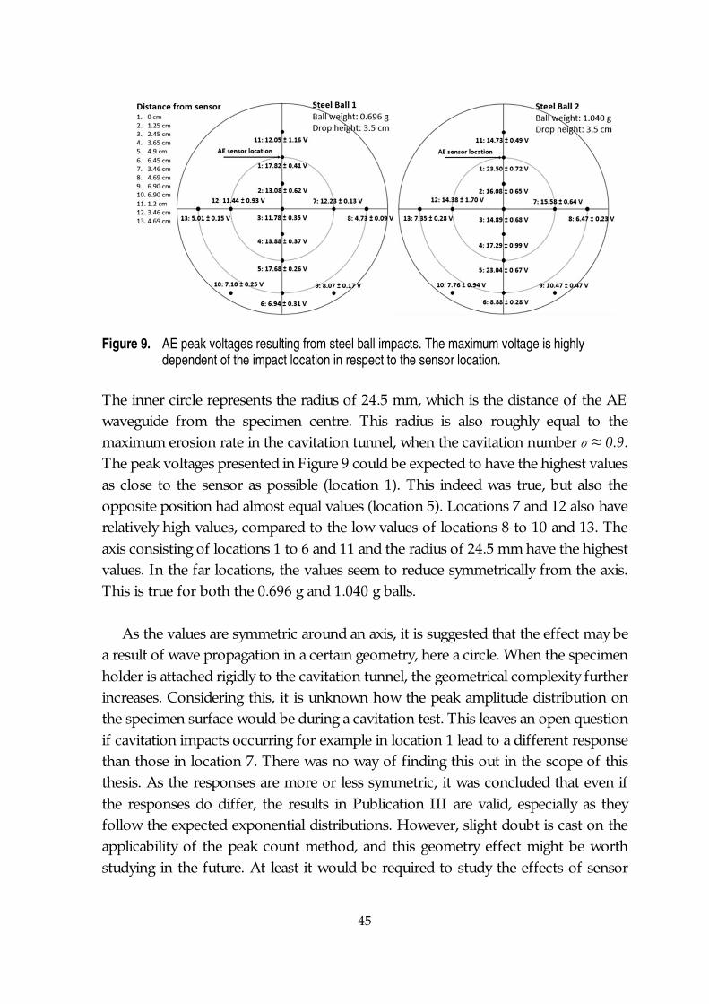
45

Figure 9. AE peak voltages resulting from steel ball impacts. The maximum voltage is highlydependent of the impact location in respect to the sensor location.

The inner circle represents the radius of 24.5 mm, which is the distance of the AEwaveguide from the specimen centre. This radius is also roughly equal to themaximum erosion rate in the cavitation tunnel, when the cavitation number σ ≈ 0.9.The peak voltages presented in Figure 9 could be expected to have the highest valuesas close to the sensor as possible (location 1). This indeed was true, but also theopposite position had almost equal values (location 5). Locations 7 and 12 also haverelatively high values, compared to the low values of locations 8 to 10 and 13. Theaxis consisting of locations 1 to 6 and 11 and the radius of 24.5 mm have the highestvalues. In the far locations, the values seem to reduce symmetrically from the axis.This is true for both the 0.696 g and 1.040 g balls.

As the values are symmetric around an axis, it is suggested that the effect may bea result of wave propagation in a certain geometry, here a circle. When the specimenholder is attached rigidly to the cavitation tunnel, the geometrical complexity furtherincreases. Considering this, it is unknown how the peak amplitude distribution onthe specimen surface would be during a cavitation test. This leaves an open questionif cavitation impacts occurring for example in location 1 lead to a different responsethan those in location 7. There was no way of finding this out in the scope of thisthesis. As the responses are more or less symmetric, it was concluded that even ifthe responses do differ, the results in Publication III are valid, especially as theyfollow the expected exponential distributions. However, slight doubt is cast on theapplicability of the peak count method, and this geometry effect might be worthstudying in the future. At least it would be required to study the effects of sensor

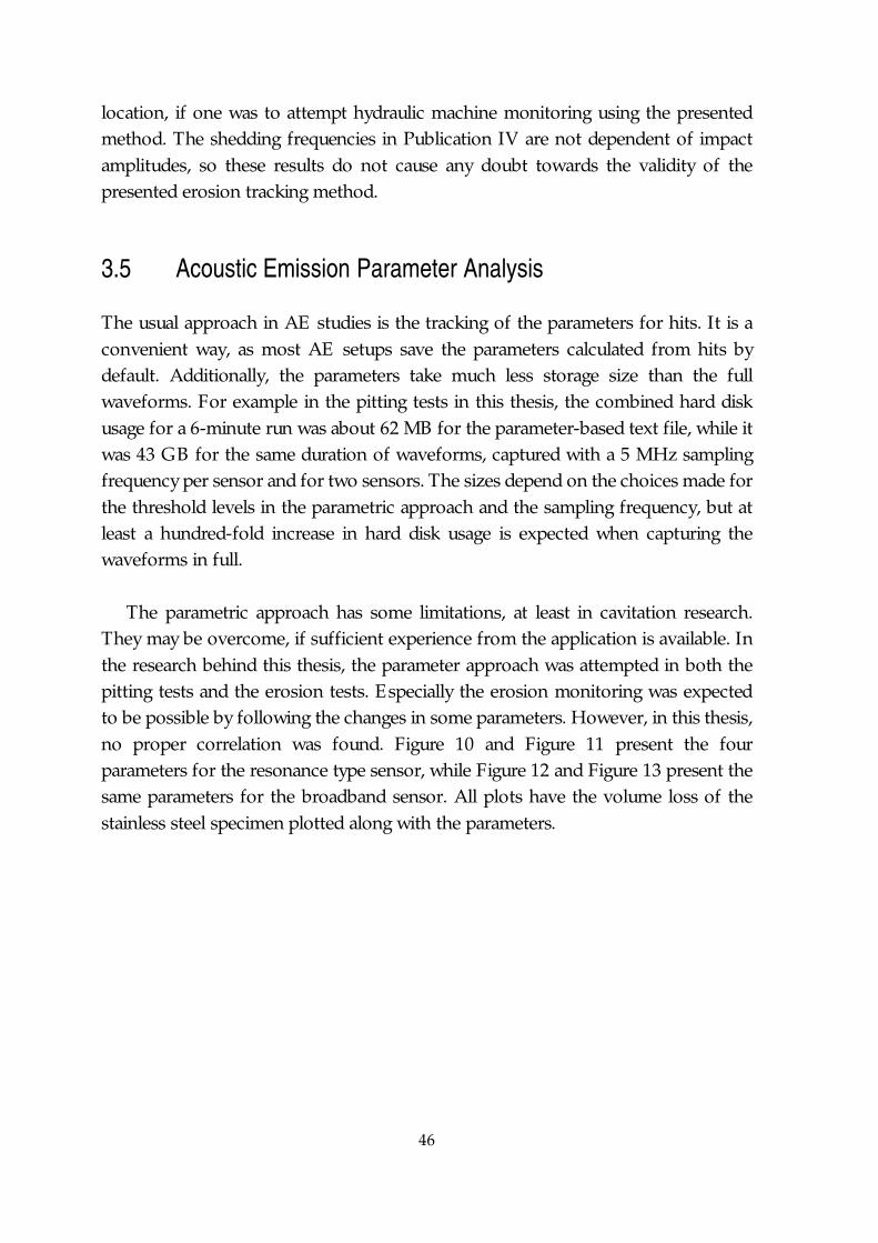
46

location, if one was to attempt hydraulic machine monitoring using the presentedmethod. The shedding frequencies in Publication IV are not dependent of impactamplitudes, so these results do not cause any doubt towards the validity of thepresented erosion tracking method.

3.5 Acoustic Emission Parameter Analysis

The usual approach in AE studies is the tracking of the parameters for hits. It is aconvenient way, as most AE setups save the parameters calculated from hits bydefault. Additionally, the parameters take much less storage size than the fullwaveforms. For example in the pitting tests in this thesis, the combined hard diskusage for a 6-minute run was about 62 MB for the parameter-based text file, while itwas 43 GB for the same duration of waveforms, captured with a 5 MHz samplingfrequency per sensor and for two sensors. The sizes depend on the choices made forthe threshold levels in the parametric approach and the sampling frequency, but atleast a hundred-fold increase in hard disk usage is expected when capturing thewaveforms in full.

The parametric approach has some limitations, at least in cavitation research.They may be overcome, if sufficient experience from the application is available. Inthe research behind this thesis, the parameter approach was attempted in both thepitting tests and the erosion tests. Especially the erosion monitoring was expectedto be possible by following the changes in some parameters. However, in this thesis,no proper correlation was found. Figure 10 and Figure 11 present the fourparameters for the resonance type sensor, while Figure 12 and Figure 13 present thesame parameters for the broadband sensor. All plots have the volume loss of thestainless steel specimen plotted along with the parameters.

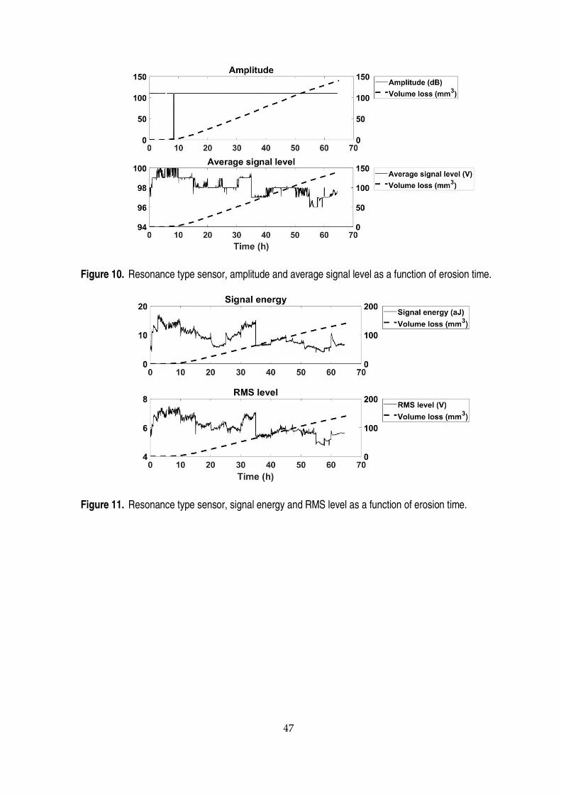
47

Figure 10. Resonance type sensor, amplitude and average signal level as a function of erosion time.

Figure 11. Resonance type sensor, signal energy and RMS level as a function of erosion time.

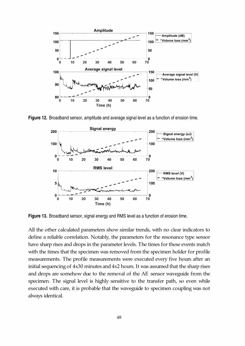
48

Figure 12. Broadband sensor, amplitude and average signal level as a function of erosion time.

Figure 13. Broadband sensor, signal energy and RMS level as a function of erosion time.

All the other calculated parameters show similar trends, with no clear indicators todefine a reliable correlation. Notably, the parameters for the resonance type sensorhave sharp rises and drops in the parameter levels. The times for these events matchwith the times that the specimen was removed from the specimen holder for profilemeasurements. The profile measurements were executed every five hours after aninitial sequencing of 4x30 minutes and 4x2 hours. It was assumed that the sharp risesand drops are somehow due to the removal of the AE sensor waveguide from thespecimen. The signal level is highly sensitive to the transfer path, so even whileexecuted with care, it is probable that the waveguide to specimen coupling was notalways identical.

49

Despite its limitations, the parametric approach has been successfully used incavitation research by other authors. The failure of the parametric approach in thisthesis proves in no way that the approach could not work. Using machine learningalgorithms, neural networks or some other approaches, the trends in the parametersmight be revealed better than in the basic analysis in this thesis. Most of the otherauthors, however, concentrated on determining cavitation occurrence and intensity,rather than erosion evolution. A good example of an advanced approach was by(Look et al. 2018), who did not predefine any features to be tracked. They usedconvolutional neural networks that were able to detect cavitation in a turbine withhigh accuracy, with an estimate of the cavitation intensity.

Another example of a successful parametric approach was by (Schmidt et al. 2014;Schmidt et al. 2015). They categorized Kaplan turbine and pump turbine cavitationinto four states from no cavitation to severe cavitation. Their experiments includedturbines fitted with AE sensors and means to observe visually the state of cavitation.The classification was based on the rise of AE energy and RMS value, and theincreased fluctuation of both, when moving towards increased cavitation. (He &Shen 2012) experimented AE and erosion evolution in the ASTM G32 vibratorycavitation testing apparatus. They also tracked the RMS value and the signal energyand they concluded that the average energy shows increase when the specimen massloss is pronounced. This relation was not found in the current study.

3.6 Cavitation Shedding Frequency Detection

As the parametric approach was found not to be suitable for the goals in this thesis,another method, based on spectrum analysis, was developed for the tracking oferosion evolution. As the cavitation produced in the tunnel in this thesis is cloudcavitation, the cavitation impacts attacking the specimen surface have a periodicnature. This was described in detail in section 2.2 and in Publication IV. Theshedding frequency in the cavitation tunnel was expected to be between a fewhundred Hz to a few kHz (Peters et al. 2015; Gavaises et al. 2015). The AE sensorsensitivity drops rapidly below 100 kHz and the preamplifiers used in this thesis hadan analogue band-pass filter with a 100 kHz lower limit and a 400 or 1200 kHz upperlimit. Additionally, the measurement system had a digital high-pass filter of a 100

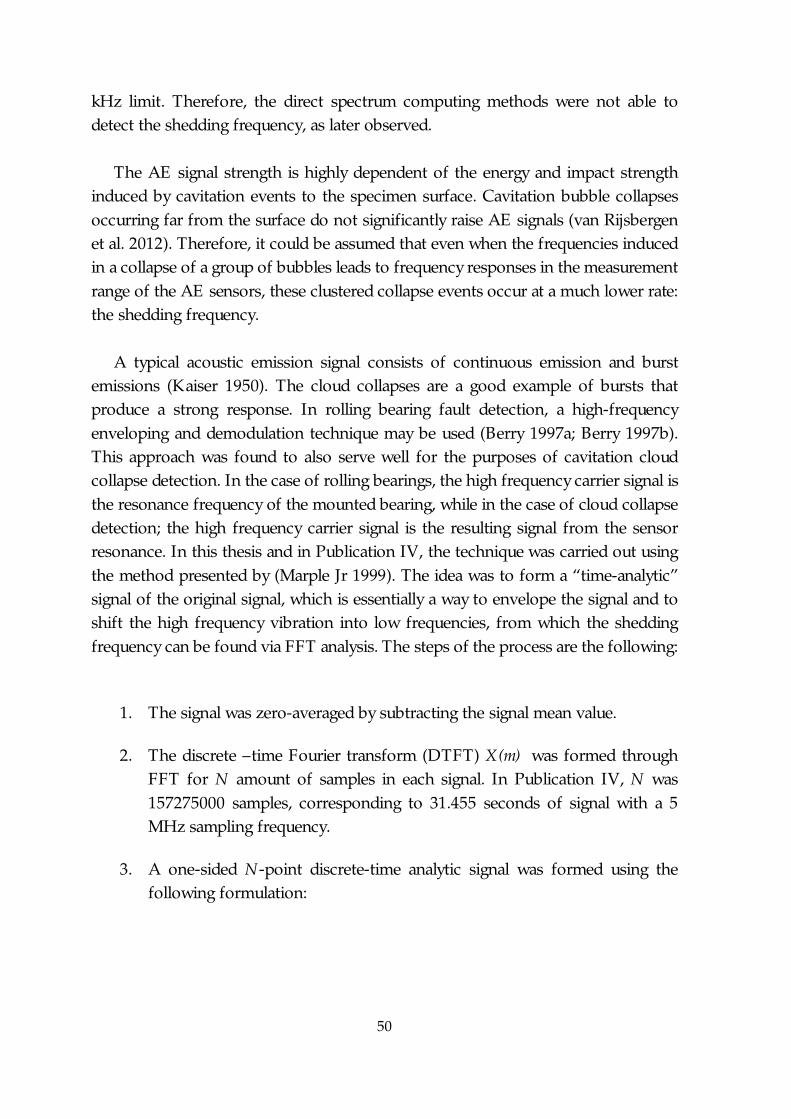
50

kHz limit. Therefore, the direct spectrum computing methods were not able todetect the shedding frequency, as later observed.

The AE signal strength is highly dependent of the energy and impact strengthinduced by cavitation events to the specimen surface. Cavitation bubble collapsesoccurring far from the surface do not significantly raise AE signals (van Rijsbergenet al. 2012). Therefore, it could be assumed that even when the frequencies inducedin a collapse of a group of bubbles leads to frequency responses in the measurementrange of the AE sensors, these clustered collapse events occur at a much lower rate:the shedding frequency.

A typical acoustic emission signal consists of continuous emission and burstemissions (Kaiser 1950). The cloud collapses are a good example of bursts thatproduce a strong response. In rolling bearing fault detection, a high-frequencyenveloping and demodulation technique may be used (Berry 1997a; Berry 1997b).This approach was found to also serve well for the purposes of cavitation cloudcollapse detection. In the case of rolling bearings, the high frequency carrier signal isthe resonance frequency of the mounted bearing, while in the case of cloud collapsedetection; the high frequency carrier signal is the resulting signal from the sensorresonance. In this thesis and in Publication IV, the technique was carried out usingthe method presented by (Marple Jr 1999). The idea was to form a “time-analytic”signal of the original signal, which is essentially a way to envelope the signal and toshift the high frequency vibration into low frequencies, from which the sheddingfrequency can be found via FFT analysis. The steps of the process are the following:

1. The signal was zero-averaged by subtracting the signal mean value.

2. The discrete –time Fourier transform (DTFT) X(m) was formed throughFFT for N amount of samples in each signal. In Publication IV, N was157275000 samples, corresponding to 31.455 seconds of signal with a 5MHz sampling frequency.

3. A one-sided N-point discrete-time analytic signal was formed using thefollowing formulation:

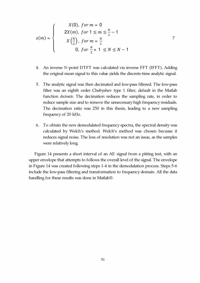
51

( ) =

⎩⎪⎨⎪⎧ (0), = 0

2 ( ), 1 ≤ ≤ − 1

, =

0, + 1 ≤ ≤ − 1

7

4. An inverse N-point DTFT was calculated via inverse FFT (IFFT). Addingthe original mean signal to this value yields the discrete-time analytic signal.

5. The analytic signal was then decimated and low-pass filtered. The low-passfilter was an eighth order Chebyshev type 1 filter, default in the Matlabfunction decimate. The decimation reduces the sampling rate, in order toreduce sample size and to remove the unnecessary high frequency residuals.The decimation ratio was 250 in this thesis, leading to a new samplingfrequency of 20 kHz.

6. To obtain the new demodulated frequency spectra, the spectral density wascalculated by Welch’s method. Welch’s method was chosen because itreduces signal noise. The loss of resolution was not an issue, as the sampleswere relatively long.

Figure 14 presents a short interval of an AE signal from a pitting test, with anupper envelope that attempts to follows the overall level of the signal. The envelopein Figure 14 was created following steps 1-4 in the demodulation process. Steps 5-6include the low-pass filtering and transformation to frequency domain. All the datahandling for these results was done in Matlab®.

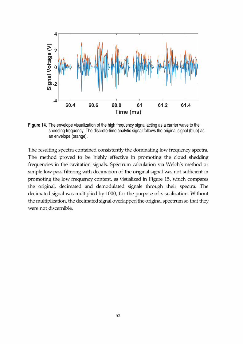
52

Figure 14. The envelope visualization of the high frequency signal acting as a carrier wave to theshedding frequency. The discrete-time analytic signal follows the original signal (blue) asan envelope (orange).

The resulting spectra contained consistently the dominating low frequency spectra.The method proved to be highly effective in promoting the cloud sheddingfrequencies in the cavitation signals. Spectrum calculation via Welch’s method orsimple low-pass filtering with decimation of the original signal was not sufficient inpromoting the low frequency content, as visualized in Figure 15, which comparesthe original, decimated and demodulated signals through their spectra. Thedecimated signal was multiplied by 1000, for the purpose of visualization. Withoutthe multiplication, the decimated signal overlapped the original spectrum so that theywere not discernible.

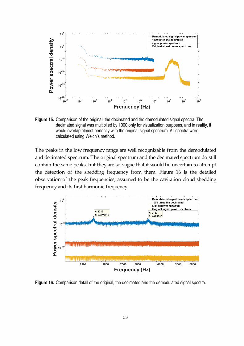
53

Figure 15. Comparison of the original, the decimated and the demodulated signal spectra. Thedecimated signal was multiplied by 1000 only for visualization purposes, and in reality, itwould overlap almost perfectly with the original signal spectrum. All spectra werecalculated using Welch’s method.

The peaks in the low frequency range are well recognizable from the demodulatedand decimated spectrum. The original spectrum and the decimated spectrum do stillcontain the same peaks, but they are so vague that it would be uncertain to attemptthe detection of the shedding frequency from them. Figure 16 is the detailedobservation of the peak frequencies, assumed to be the cavitation cloud sheddingfrequency and its first harmonic frequency.

Figure 16. Comparison detail of the original, the decimated and the demodulated signal spectra.

54

The decimation process includes the low-pass filtering of the original signal. It isclear from the previous figures that this is an insufficient approach, while thedemodulation, which is effectively enveloping combined with decimation, providesgood results in terms of promoting low frequency contents. This was the approachin Publication IV, also described in section 5.4.

55

4 METHODOLOGY AND EXPERIMENTS

4.1 The PREVERO Cavitation Tunnel

All the main results in this thesis were obtained from experiments with thePREVERO cavitation tunnel that is situated in the LEGI laboratory, in Grenoble,France (PREVERO 2018). The tunnel is mostly utilized in cavitation erosion testing,in either short-duration pitting tests, or long-duration erosion tests. The duration ofthe tests is highly dependent of the specimen material and the tunnel operation point.The tunnel circulates water through a test section, with the possibility to control thepressure downstream of the test section by a pressurized nitrogen tank and upstreamby a pump that has a frequency regulator to control rotation speed. The tunneloperation is thoroughly explained in Publications II, III and IV, and in (Franc 2009;Ylönen 2016). This section, however, also explains the basic operation.

The material specimens are 20 mm thick and 100 mm diameter cylinders thathave a polished circular face towards the flow. The other face is towards thespecimen holder, and it has a screw thread for fixing it to place. A 16 mm diameternozzle feeds water to the test section that is a radially diverging channel of 2.5 mmthickness. The water jet from the nozzle stagnates in the middle of the materialspecimen and the water flow turns 90 degrees and begins to flow in all directions inthe plane. Cavitation inception occurs as the flow cross-section area drops to 62.5% at 8 mm radius, where the nozzle ends and the 2.5 mm thick channel begins. Asthe channel further diverges and the cross-section area increases, the static pressurealso increases and the formed cavitation clouds collapse and damage the sample, inthe area between 19 mm and 32 mm radius.

The flow velocity in the cavitating area and in the nozzle are major contributorsto the aggressiveness of the cavitation field. The relevant velocity is the referencevelocity calculated from the Bernoulli equation, assuming that the pressure inside thecavitation cloud is the vapor pressure. The vapor pressure is negligent compared tothe upstream pressure, so the cavity velocity V c may be calculated from: (Franc 2009)

56

≈ 8

where pu is the upstream pressure of the tunnel and ρw is the water density. Theerosion tests were conducted with a 4 MPa upstream pressure in this thesis, whichis the maximum allowed pressure. This corresponds to approximately 90 m/s cavityvelocity. The 2 MPa upstream pressure used in the other pitting test corresponds toa cavity velocity of about 63 m/s. (Franc et al. 2012) reported the followingdependency between coverage time τ and cavity velocity V c:

~ . 9

The coverage time is the theoretical time that would be taken for a surfaceexperiencing cavitation to be totally covered once by non-overlapping pits. Inpractice, it is calculated through a pitting test where only separate pits are formed.For example, if a surface would be covered 10 % in area with pits in 2 minutes, thecoverage time would be 20 minutes. The coverage time is linked to the erosion rate,the exact relation being dependent on the cavitation erosion test setup (Hammitt1979; Zhou & Hammitt 1983; Franc 2009). For this thesis, it is sufficient to estimatethe aggressiveness to have roughly the same dependency as the coverage time. Asthe cavity velocity is dependent of the square root of the upstream pressure, thecoverage time is dependent on the upstream pressure as:

~ ( . ) . = . 10

The 4 MPa upstream pressure is double the 2 MPa upstream pressure. Therefore,it has a coverage time of 2 . ≈ 0.11 times the coverage time of the 2 MPapressure. This means that the 4 MPa operation point is about 10 times moreaggressive than the 2 MPa operation point. The cavitation number in the tunnel isdefined as:

= 11

where pd is the downstream pressure and pv is the saturated vapor pressure.Generally pv is negligible and therefore left out from the calculation. A constantcavitation number, regardless of the pressure levels, leads to same type of cavitationand the same closure point in the diverging channel (Gavaises et al. 2015). The

57

cavitation number is related to the occurrence of cavitation and it has no well-definedconnection with the erosive potential.

4.2 Acoustic Emission Setups

The choice of acoustic emission setup has a large influence on the applicability ofthe results. In this thesis, the most important functionality was the recording of longfull waveforms with a high sampling frequency. The most important results inPublications III and IV rely on waveforms recorded continuously for up to 6minutes, with 5 MHz sampling frequency per sensor, and with two sensors. For theresonance type sensor, which had bandwidth of 100 kHz to 400 kHz, the samplingfrequency was overly sufficient. The broadband sensor had a bandwidth of 100 kHzto 900 kHz, but in the upper range, no significant information was found. Therefore,probably the same results would have been obtained using for example a 2 MHzsampling frequency.

The initial setup used in (Ylönen 2016) was an IOtech WaveBook/512, which isa system having a 12-bit voltage resolution and a maximum sampling frequency of 1MHz. One of the main limitations in that system was the limited acquisition time of30 seconds with the maximum sampling frequency, after which the system requiredseveral minutes to save the data. The other severe limitation was that the signaltended to saturate, as cavitation induced a much higher AE signal than in the usualapplications that the system was designed for. The original fix for this was to utilizea 550 kΩ resistance in the signal electrical circuit. This is a highly suspicious way tocontrol the saturation problem, as the additional resistor might modify the signalshape with no true possibilities to estimate how. Fortunately, a new acquisitionsystem solved both the problems.

The setup used in all the results listed in this thesis was a PAC PCI-2 acquisitionsystem. It had an 18-bit voltage resolution and a maximum sampling frequency of40 MHz. Continuous waveform acquisition was possible with either 10 MHzsampling with one sensor, or divided to two sensors, 5 MHz each. The sensors hadPAC 2/4/6 preamplifiers, with the 20 dB amplification option always chosen forthese measurements. The acquisition system had a PCI express connection to a 1TB SSD hard drive, allowing direct saving to the drive. The practical upper limit tothe size of waveform files was about 7 minutes, as overly large stream files were

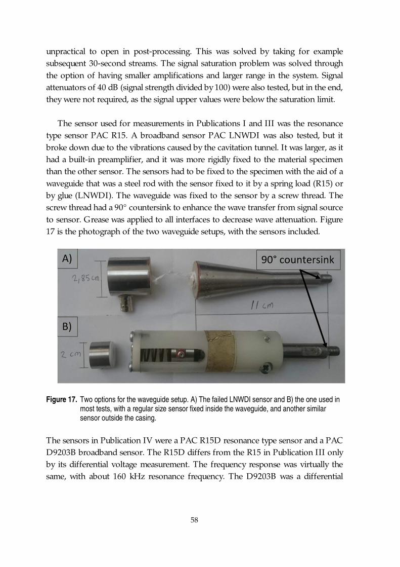
58

unpractical to open in post-processing. This was solved by taking for examplesubsequent 30-second streams. The signal saturation problem was solved throughthe option of having smaller amplifications and larger range in the system. Signalattenuators of 40 dB (signal strength divided by 100) were also tested, but in the end,they were not required, as the signal upper values were below the saturation limit.

The sensor used for measurements in Publications I and III was the resonancetype sensor PAC R15. A broadband sensor PAC LNWDI was also tested, but itbroke down due to the vibrations caused by the cavitation tunnel. It was larger, as ithad a built-in preamplifier, and it was more rigidly fixed to the material specimenthan the other sensor. The sensors had to be fixed to the specimen with the aid of awaveguide that was a steel rod with the sensor fixed to it by a spring load (R15) orby glue (LNWDI). The waveguide was fixed to the sensor by a screw thread. Thescrew thread had a 90° countersink to enhance the wave transfer from signal sourceto sensor. Grease was applied to all interfaces to decrease wave attenuation. Figure17 is the photograph of the two waveguide setups, with the sensors included.

Figure 17. Two options for the waveguide setup. A) The failed LNWDI sensor and B) the one used inmost tests, with a regular size sensor fixed inside the waveguide, and another similarsensor outside the casing.

The sensors in Publication IV were a PAC R15D resonance type sensor and a PACD9203B broadband sensor. The R15D differs from the R15 in Publication III onlyby its differential voltage measurement. The frequency response was virtually thesame, with about 160 kHz resonance frequency. The D9203B was a differential

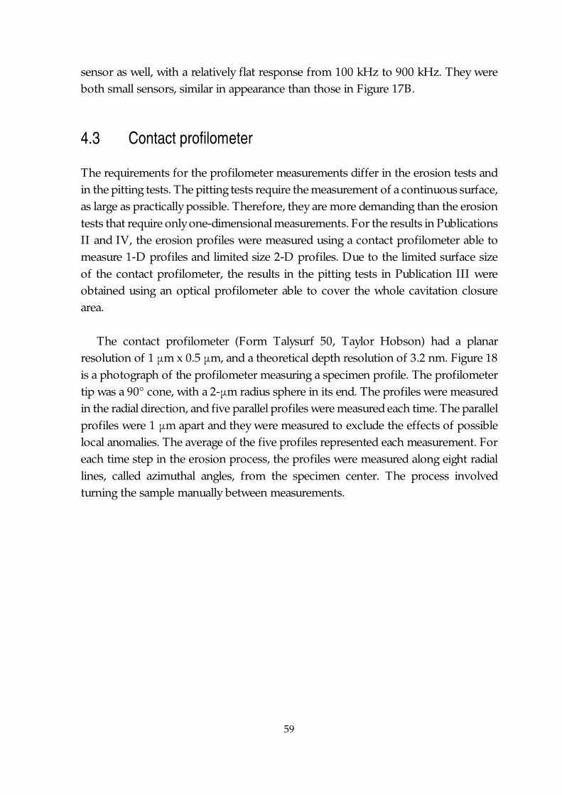
59

sensor as well, with a relatively flat response from 100 kHz to 900 kHz. They wereboth small sensors, similar in appearance than those in Figure 17B.

4.3 Contact profilometer

The requirements for the profilometer measurements differ in the erosion tests andin the pitting tests. The pitting tests require the measurement of a continuous surface,as large as practically possible. Therefore, they are more demanding than the erosiontests that require only one-dimensional measurements. For the results in PublicationsII and IV, the erosion profiles were measured using a contact profilometer able tomeasure 1-D profiles and limited size 2-D profiles. Due to the limited surface sizeof the contact profilometer, the results in the pitting tests in Publication III wereobtained using an optical profilometer able to cover the whole cavitation closurearea.

The contact profilometer (Form Talysurf 50, Taylor Hobson) had a planarresolution of 1 μm x 0.5 μm, and a theoretical depth resolution of 3.2 nm. Figure 18is a photograph of the profilometer measuring a specimen profile. The profilometertip was a 90° cone, with a 2-μm radius sphere in its end. The profiles were measuredin the radial direction, and five parallel profiles were measured each time. The parallelprofiles were 1 μm apart and they were measured to exclude the effects of possiblelocal anomalies. The average of the five profiles represented each measurement. Foreach time step in the erosion process, the profiles were measured along eight radiallines, called azimuthal angles, from the specimen center. The process involvedturning the sample manually between measurements.

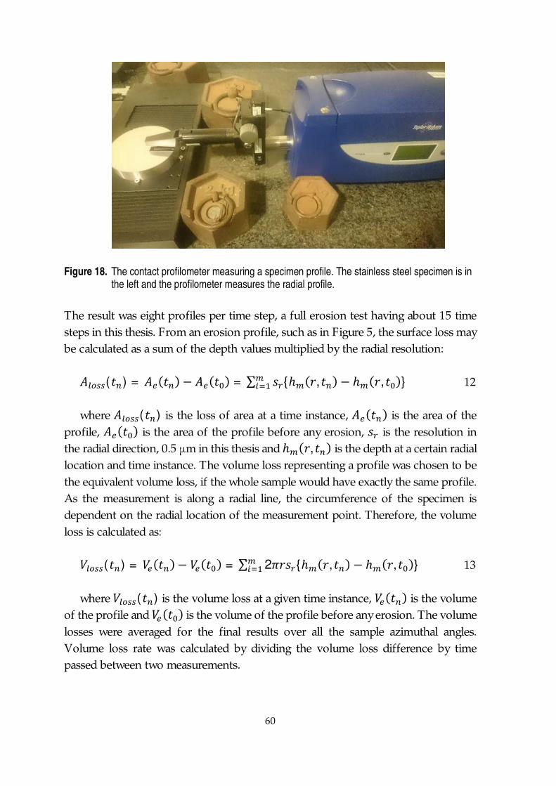
60

Figure 18. The contact profilometer measuring a specimen profile. The stainless steel specimen is inthe left and the profilometer measures the radial profile.

The result was eight profiles per time step, a full erosion test having about 15 timesteps in this thesis. From an erosion profile, such as in Figure 5, the surface loss maybe calculated as a sum of the depth values multiplied by the radial resolution:

( ) = ( ) − ( ) = ∑ {ℎ ( , ) − ℎ ( , )} 12

where ( ) is the loss of area at a time instance, ( ) is the area of theprofile, ( ) is the area of the profile before any erosion, is the resolution inthe radial direction, 0.5 μm in this thesis andℎ ( , ) is the depth at a certain radiallocation and time instance. The volume loss representing a profile was chosen to bethe equivalent volume loss, if the whole sample would have exactly the same profile.As the measurement is along a radial line, the circumference of the specimen isdependent on the radial location of the measurement point. Therefore, the volumeloss is calculated as:

( ) = ( ) − ( ) = ∑ 2 {ℎ ( , ) − ℎ ( , )} 13

where ( ) is the volume loss at a given time instance, ( ) is the volumeof the profile and ( ) is the volume of the profile before any erosion. The volumelosses were averaged for the final results over all the sample azimuthal angles.Volume loss rate was calculated by dividing the volume loss difference by timepassed between two measurements.

61

4.4 Optical profilometer

The contact profilometer was found to be efficient in the erosion profilemeasurements, as described in section 4.3. In measuring pitting patterns, the practicalmaximum area was about 4 mm x 4 mm with a 1 μm x 1 μm resolution measurementgrid. An optical profilometer (Alicona Infinitefocus G5) was also available and it hadthe possibility of scanning larger areas than these. Using a 3.5226 μm x 3.5226 μmmeasurement grid, the entire impacted area of the specimen could be measured.What was lost in resolution was gained in covered area. It was also found that in thepitting tests, the pit coverage rate was not axisymmetric, as visualized in PublicationIII. As the AE measurements are assumed to detect all cavitation impacts, detectingall pits in the specimen was beneficial in determining the relation between AE andpit diameters.

The basic functionality of the optical profilometer is that it has a charge-coupleddevice (CCD) camera combined with a microscope. The specimens were illuminatedby a white light source and the reflected light revealed the surface topology.Changing the vertical focal position enhanced the images, making them sharper. Asthe surface was initially polished, the profilometer failed to measure the depth valuesof the non-eroded surface. Fortunately, the pits were well captured, as they were lessreflective and they had distinguishable shapes.

The profilometer generated text files that contained the depth information alongwith location of all the measured points, but it excluded the non-eroded points thatwere not captured. As the code to detect pits from the surface expected continuousmeasurement data, the non-eroded areas had to be interpolated between successivemeasured points. After the interpolation process, the surface was divided intorectangles of less than 1 mm2, with shapes as close to a square as possible. This wasdone to reduce file size and to rectify locally the surface to be horizontal. The wholespecimen was slightly curved, so rectifying the specimen plane at once to behorizontal would not work. A local plane rectification of each small area led tovirtually no error.

After the profilometer-generated surface profiles were rectified and modified tobe compatible with the pit detection code, each pit was detected and characterized.The pit detection code was used to analyse the less than 1 mm2 surfaces. It requireda user defined depth threshold, which was chosen as 0.5 μm, following the example

62

of (Franc 2009). The pit detection code then calculated the mean depth level anddetected areas that were more than the depth threshold below the mean level. Theimage generated with these definitions was turned to binary. A disk with a radius oftwo pixels was used as the structuring element of morphological closing of the image.After these steps, the pit boundaries were detected and pit surface area, maximumdepth, volume, and circularity were calculated. The circularity is a parameter thatdefines a shapes closeness to circle. This was used to omit scratches, which have amuch lower circularity than pits caused by cavitation impacts. After the detection ofpits, the pit depths were corrected by calculating the non-eroded surface level andadding it to the pit depths calculated initially. All the data were treated in Matlab®.

4.5 Microscopy and EBSD

The erosion rate tests answer the question of how the materials compare in theircavitation erosion resistance. They however do not answer the question of why.Between very different materials, this might be answered easily. For example, it isexpected that a soft plastic would be inferior to stainless steels, as its mechanicalstrength is in every way inferior. Pure aluminum is also weaker than stainless steel inmost ways, as also in its resistance to cavitation. However, comparing two stainlesssteels with a similar yield stress and other macroscopic mechanical properties, butwith differing erosion rates, requires studies that are more advanced. This was thecase with the stainless steels in this thesis, as explained more in section 5.1 and inPublications II and V. Publication II included also the erosion testing of a low-alloysteel, which was compared to others in erosion rates, but was not interesting enoughto properly study its microstructure.

The first approach was to film the eroded and non-eroded specimen surface bySEM. The SEM images provided insight on the erosion process, but they were aloneinsufficient in determining the differences between two materials that are similar inmany ways. The SEM imaging of the eroded material surface was studied inPublication II. The SEM image analysis, however, did not provide the reasonsbehind the erosion rates. In the next step, which could have as well been the firstone, the stainless steels specimens were etched and imaged through conventionalmicroscopy.

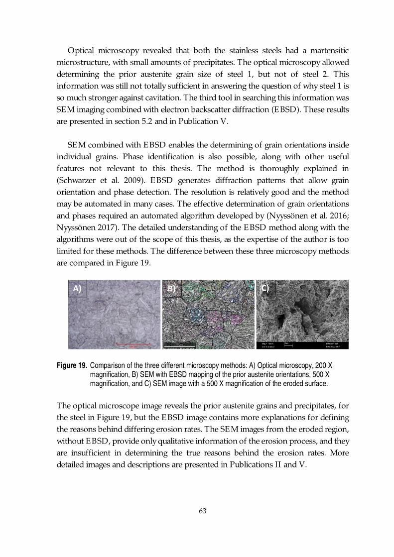
63

Optical microscopy revealed that both the stainless steels had a martensiticmicrostructure, with small amounts of precipitates. The optical microscopy alloweddetermining the prior austenite grain size of steel 1, but not of steel 2. Thisinformation was still not totally sufficient in answering the question of why steel 1 isso much stronger against cavitation. The third tool in searching this information wasSEM imaging combined with electron backscatter diffraction (EBSD). These resultsare presented in section 5.2 and in Publication V.

SEM combined with EBSD enables the determining of grain orientations insideindividual grains. Phase identification is also possible, along with other usefulfeatures not relevant to this thesis. The method is thoroughly explained in(Schwarzer et al. 2009). EBSD generates diffraction patterns that allow grainorientation and phase detection. The resolution is relatively good and the methodmay be automated in many cases. The effective determination of grain orientationsand phases required an automated algorithm developed by (Nyyssönen et al. 2016;Nyyssönen 2017). The detailed understanding of the EBSD method along with thealgorithms were out of the scope of this thesis, as the expertise of the author is toolimited for these methods. The difference between these three microscopy methodsare compared in Figure 19.

Figure 19. Comparison of the three different microscopy methods: A) Optical microscopy, 200 Xmagnification, B) SEM with EBSD mapping of the prior austenite orientations, 500 Xmagnification, and C) SEM image with a 500 X magnification of the eroded surface.

The optical microscope image reveals the prior austenite grains and precipitates, forthe steel in Figure 19, but the EBSD image contains more explanations for definingthe reasons behind differing erosion rates. The SEM images from the eroded region,without EBSD, provide only qualitative information of the erosion process, and theyare insufficient in determining the true reasons behind the erosion rates. Moredetailed images and descriptions are presented in Publications II and V.

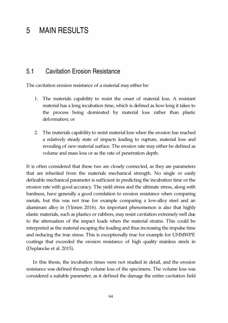
64

5 MAIN RESULTS

5.1 Cavitation Erosion Resistance

The cavitation erosion resistance of a material may either be:

1. The materials capability to resist the onset of material loss. A resistantmaterial has a long incubation time, which is defined as how long it takes tothe process being dominated by material loss rather than plasticdeformation; or

2. The materials capability to resist material loss when the erosion has reacheda relatively steady state of impacts leading to rupture, material loss andrevealing of new material surface. The erosion rate may either be defined asvolume and mass loss or as the rate of penetration depth.

It is often considered that these two are closely connected, as they are parametersthat are inherited from the materials mechanical strength. No single or easilydefinable mechanical parameter is sufficient in predicting the incubation time or theerosion rate with good accuracy. The yield stress and the ultimate stress, along withhardness, have generally a good correlation to erosion resistance when comparingmetals, but this was not true for example comparing a low-alloy steel and analuminum alloy in (Ylönen 2016). An important phenomenon is also that highlyelastic materials, such as plastics or rubbers, may resist cavitation extremely well dueto the attenuation of the impact loads when the material strains. This could beinterpreted as the material escaping the loading and thus increasing the impulse timeand reducing the true stress. This is exceptionally true for example for UHMWPEcoatings that exceeded the erosion resistance of high quality stainless steels in(Deplancke et al. 2015).

In this thesis, the incubation times were not studied in detail, and the erosionresistance was defined through volume loss of the specimens. The volume loss wasconsidered a suitable parameter, as it defined the damage the entire cavitation field

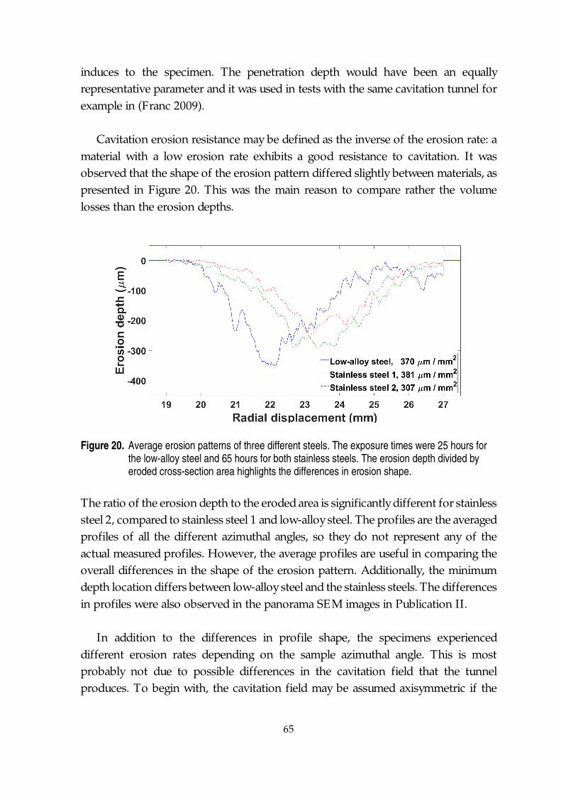
65

induces to the specimen. The penetration depth would have been an equallyrepresentative parameter and it was used in tests with the same cavitation tunnel forexample in (Franc 2009).

Cavitation erosion resistance may be defined as the inverse of the erosion rate: amaterial with a low erosion rate exhibits a good resistance to cavitation. It wasobserved that the shape of the erosion pattern differed slightly between materials, aspresented in Figure 20. This was the main reason to compare rather the volumelosses than the erosion depths.

Figure 20. Average erosion patterns of three different steels. The exposure times were 25 hours forthe low-alloy steel and 65 hours for both stainless steels. The erosion depth divided byeroded cross-section area highlights the differences in erosion shape.

The ratio of the erosion depth to the eroded area is significantly different for stainlesssteel 2, compared to stainless steel 1 and low-alloy steel. The profiles are the averagedprofiles of all the different azimuthal angles, so they do not represent any of theactual measured profiles. However, the average profiles are useful in comparing theoverall differences in the shape of the erosion pattern. Additionally, the minimumdepth location differs between low-alloy steel and the stainless steels. The differencesin profiles were also observed in the panorama SEM images in Publication II.

In addition to the differences in profile shape, the specimens experienceddifferent erosion rates depending on the sample azimuthal angle. This is mostprobably not due to possible differences in the cavitation field that the tunnelproduces. To begin with, the cavitation field may be assumed axisymmetric if the

66

feed nozzle is not overly damaged. Additionally, the specimens were turned 90degrees after every time that they were removed from the tunnel for profilemeasurements. Therefore, the discrepancies in the cavitation field fromaxisymmetric shape would be negated in the end. The volume losses for the threestudied materials, with all the azimuthal angles, are plotted in Figure 21.

Figure 21. Volume loss dependency on azimuthal angle. The azimuthal angle is explained in section2.4.

As the plots overlap significantly, it would be difficult to mark the azimuthal anglesin the figure. Therefore, the final volume losses are presented in Table 1. Its mainpurpose is to support Figure 21, as the volume loss rates in Table 2 represent betterthe erosion resistances of the materials.

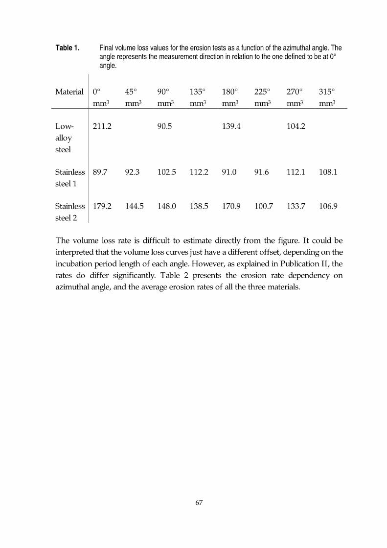
67

Table 1. Final volume loss values for the erosion tests as a function of the azimuthal angle. Theangle represents the measurement direction in relation to the one defined to be at 0°angle.

Material 0°mm3

45°mm3

90°mm3

135°mm3

180°mm3

225°mm3

270°mm3

315°mm3

Low-alloysteel

211.2 90.5 139.4 104.2

Stainlesssteel 1

89.7 92.3 102.5 112.2 91.0 91.6 112.1 108.1

Stainlesssteel 2

179.2 144.5 148.0 138.5 170.9 100.7 133.7 106.9

The volume loss rate is difficult to estimate directly from the figure. It could beinterpreted that the volume loss curves just have a different offset, depending on theincubation period length of each angle. However, as explained in Publication II, therates do differ significantly. Table 2 presents the erosion rate dependency onazimuthal angle, and the average erosion rates of all the three materials.

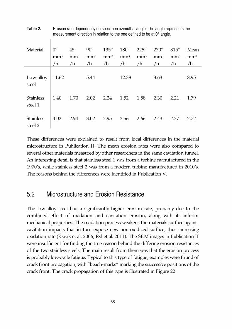
68

Table 2. Erosion rate dependency on specimen azimuthal angle. The angle represents themeasurement direction in relation to the one defined to be at 0° angle.

Material 0°mm3

/h

45°mm3

/h

90°mm3

/h

135°mm3

/h

180°mm3

/h

225°mm3

/h

270°mm3

/h

315°mm3

/h

Meanmm3

/h

Low-alloysteel

11.62 5.44 12.38 3.63 8.95

Stainlesssteel 1

1.40 1.70 2.02 2.24 1.52 1.58 2.30 2.21 1.79

Stainlesssteel 2

4.02 2.94 3.02 2.95 3.56 2.66 2.43 2.27 2.72

These differences were explained to result from local differences in the materialmicrostructure in Publication II. The mean erosion rates were also compared toseveral other materials measured by other researchers in the same cavitation tunnel.An interesting detail is that stainless steel 1 was from a turbine manufactured in the1970’s, while stainless steel 2 was from a modern turbine manufactured in 2010’s.The reasons behind the differences were identified in Publication V.

5.2 Microstructure and Erosion Resistance

The low-alloy steel had a significantly higher erosion rate, probably due to thecombined effect of oxidation and cavitation erosion, along with its inferiormechanical properties. The oxidation process weakens the materials surface againstcavitation impacts that in turn expose new non-oxidized surface, thus increasingoxidation rate (Kwok et al. 2006; Ryl et al. 2011). The SEM images in Publication IIwere insufficient for finding the true reason behind the differing erosion resistancesof the two stainless steels. The main result from them was that the erosion processis probably low-cycle fatigue. Typical to this type of fatigue, examples were found ofcrack front propagation, with “beach-marks” marking the successive positions of thecrack front. The crack propagation of this type is illustrated in Figure 22.

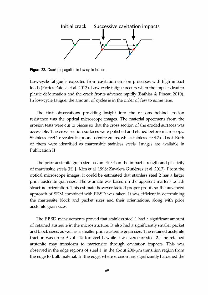
69

Figure 22. Crack propagation in low-cycle fatigue.

Low-cycle fatigue is expected from cavitation erosion processes with high impactloads (Fortes Patella et al. 2013). Low-cycle fatigue occurs when the impacts lead toplastic deformation and the crack fronts advance rapidly (Bathias & Pineau 2010).In low-cycle fatigue, the amount of cycles is in the order of few to some tens.

The first observations providing insight into the reasons behind erosionresistance was the optical microscope images. The material specimens from theerosion tests were cut to pieces so that the cross section of the eroded surfaces wasaccessible. The cross section surfaces were polished and etched before microscopy.Stainless steel 1 revealed its prior austenite grains, while stainless steel 2 did not. Bothof them were identified as martensitic stainless steels. Images are available inPublication II.

The prior austenite grain size has an effect on the impact strength and plasticityof martensitic steels (H. J. Kim et al. 1998; Zavaleta Gutiérrez et al. 2013). From theoptical microscope images, it could be estimated that stainless steel 2 has a largerprior austenite grain size. The estimate was based on the apparent martensite lathstructure orientation. This estimate however lacked proper proof, so the advancedapproach of SEM combined with EBSD was taken. It was efficient in determiningthe martensite block and packet sizes and their orientations, along with prioraustenite grain sizes.

The EBSD measurements proved that stainless steel 1 had a significant amountof retained austenite in the microstructure. It also had a significantly smaller packetand block sizes, as well as a smaller prior austenite grain size. The retained austenitefraction was up to 9 vol - % for steel 1, while it was zero for steel 2. The retainedaustenite may transform to martensite through cavitation impacts. This wasobserved in the edge regions of steel 1, in the about 200-μm transition region fromthe edge to bulk material. In the edge, where erosion has significantly hardened the

70

material, all the austenite had transformed to martensite. The transition region depthcorrelates well with that measured by (Berchiche et al. 2002), who measured thehardened layer by micro-hardness measurements for a 316L specimen that hadexperienced cavitation erosion.

The interesting thing about the microstructure of steel 1 is that it resembles thatof steels that have been processed by quenching and partitioning (Q&P). The Q&Pprocess was not a known process, according to (Edmonds et al. 2006), before 2006.However, steel 1 was from a turbine manufactured in the 1970’s. This indicates thatthe Q&P microstructure was perhaps accidentally achieved for the steel, or that someother treatment has provided a similar microstructure. The further analysis of thesefactors are far beyond the scope of this thesis. It may be however concluded that themicrostructure for stainless steel 1, presented in Publication V, is a desired one inmanufacturing cavitation resistant steels.

5.3 Defining Cavitation Intensity by Acoustic Emission

The main result in this thesis relating to the estimation of the impacts strengths wasdiscussed in Publication III. Publication I presents the basic principles in utilizingAE in cavitation testing and in using the enveloping method to detect peaks anddetermine their amplitudes. Publication III combined this information to pitdistributions and presented a correlation between AE peak voltage value and pitdiameter. The cumulative pit diameters and the peak voltage values both had a longlinear range in the linear – logarithmic scale. Normalizing pit diameters with thereference pit diameter, explained in section 2.3, and then normalizing also AE peakvoltage values with the reference peak voltage value led to almost overlappingcumulative distributions. When corrected by first subtracting the cut-off voltagefrom the voltage values, the distributions overlapped almost perfectly. Thenormalized, overlapping cumulative distributions are presented in Figure 23. Thevoltage values below the cut-off limit were omitted, as they are assumed to be eitherfrom noise or from non-damaging impacts.

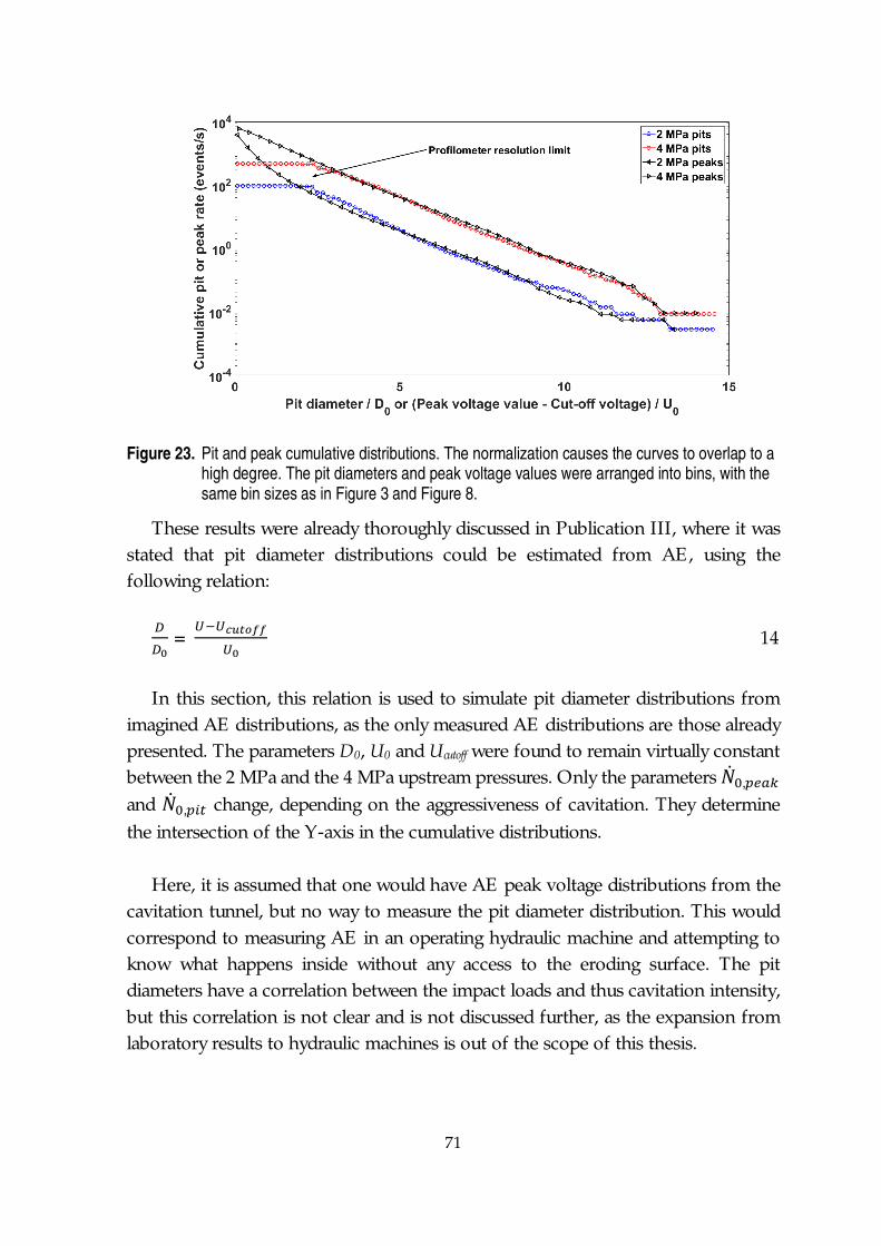
71

Figure 23. Pit and peak cumulative distributions. The normalization causes the curves to overlap to ahigh degree. The pit diameters and peak voltage values were arranged into bins, with thesame bin sizes as in Figure 3 and Figure 8.

These results were already thoroughly discussed in Publication III, where it wasstated that pit diameter distributions could be estimated from AE, using thefollowing relation:

= 14

In this section, this relation is used to simulate pit diameter distributions fromimagined AE distributions, as the only measured AE distributions are those alreadypresented. The parameters D0, U0 and Ucutoff were found to remain virtually constantbetween the 2 MPa and the 4 MPa upstream pressures. Only the parameters ,

and , change, depending on the aggressiveness of cavitation. They determinethe intersection of the Y-axis in the cumulative distributions.

Here, it is assumed that one would have AE peak voltage distributions from thecavitation tunnel, but no way to measure the pit diameter distribution. This wouldcorrespond to measuring AE in an operating hydraulic machine and attempting toknow what happens inside without any access to the eroding surface. The pitdiameters have a correlation between the impact loads and thus cavitation intensity,but this correlation is not clear and is not discussed further, as the expansion fromlaboratory results to hydraulic machines is out of the scope of this thesis.

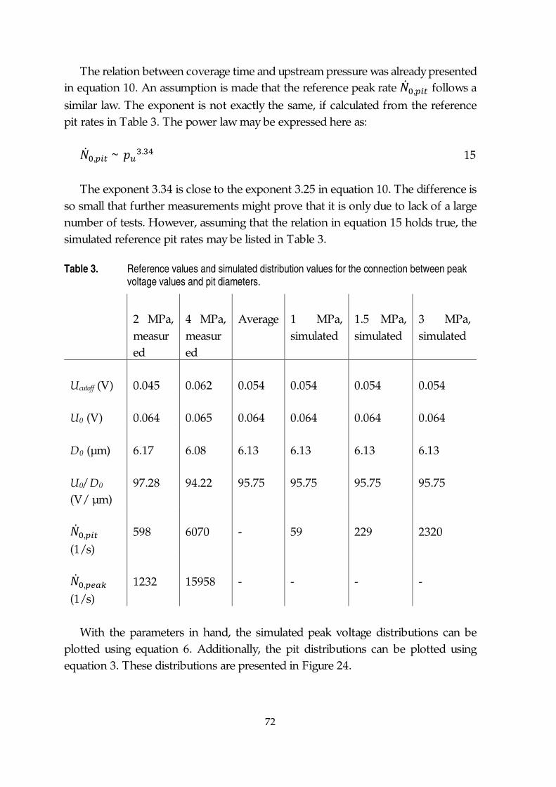
72

The relation between coverage time and upstream pressure was already presentedin equation 10. An assumption is made that the reference peak rate , follows a

similar law. The exponent is not exactly the same, if calculated from the referencepit rates in Table 3. The power law may be expressed here as: , ~ . 15

The exponent 3.34 is close to the exponent 3.25 in equation 10. The difference isso small that further measurements might prove that it is only due to lack of a largenumber of tests. However, assuming that the relation in equation 15 holds true, thesimulated reference pit rates may be listed in Table 3.

Table 3. Reference values and simulated distribution values for the connection between peakvoltage values and pit diameters.

2 MPa,measured

4 MPa,measured

Average 1 MPa,simulated

1.5 MPa,simulated

3 MPa,simulated

Ucutoff (V) 0.045 0.062 0.054 0.054 0.054 0.054

U0 (V) 0.064 0.065 0.064 0.064 0.064 0.064

D0 (µm) 6.17 6.08 6.13 6.13 6.13 6.13

U0/ D0

(V/ µm)97.28 94.22 95.75 95.75 95.75 95.75

,

(1/s)598 6070 - 59 229 2320

,

(1/s)1232 15958 - - - -

With the parameters in hand, the simulated peak voltage distributions can beplotted using equation 6. Additionally, the pit distributions can be plotted usingequation 3. These distributions are presented in Figure 24.

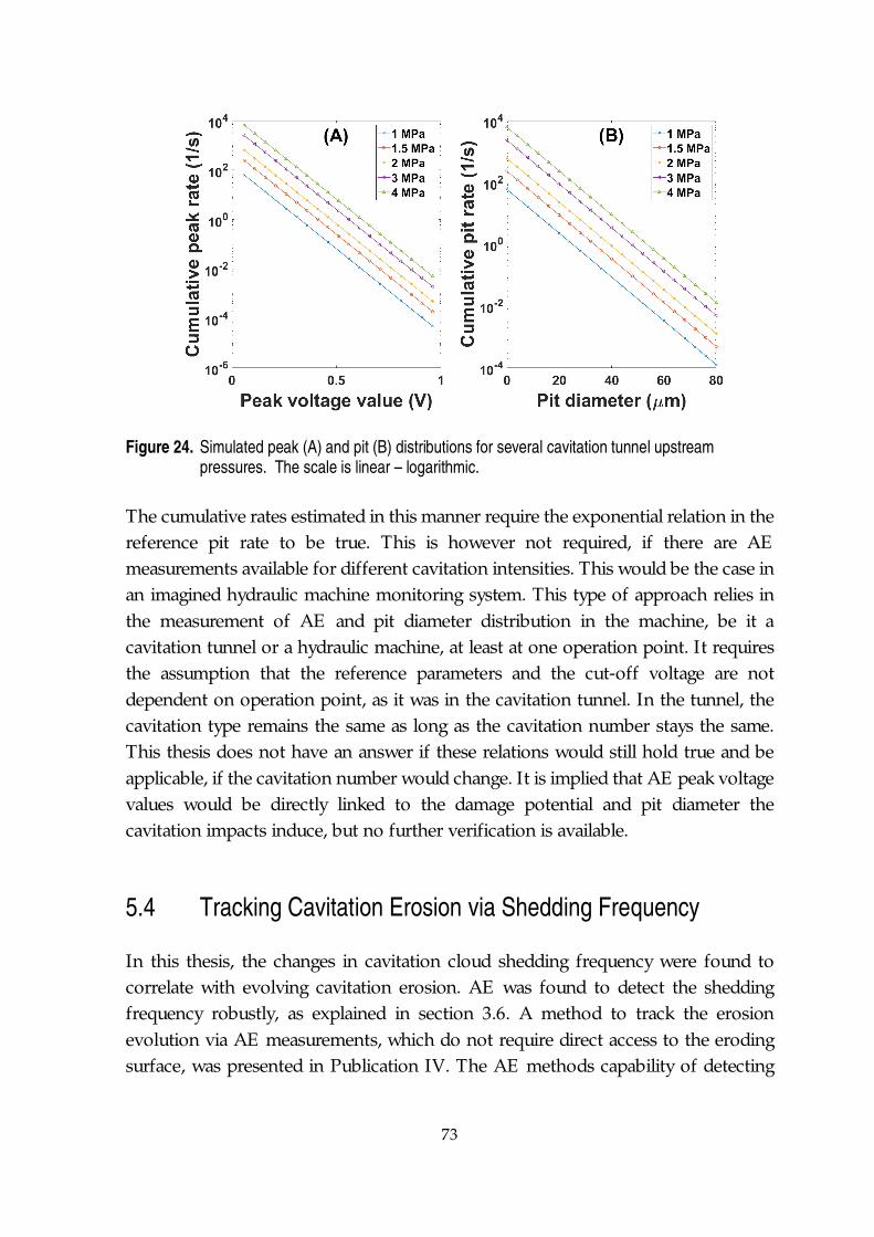
73

Figure 24. Simulated peak (A) and pit (B) distributions for several cavitation tunnel upstreampressures. The scale is linear – logarithmic.

The cumulative rates estimated in this manner require the exponential relation in thereference pit rate to be true. This is however not required, if there are AEmeasurements available for different cavitation intensities. This would be the case inan imagined hydraulic machine monitoring system. This type of approach relies inthe measurement of AE and pit diameter distribution in the machine, be it acavitation tunnel or a hydraulic machine, at least at one operation point. It requiresthe assumption that the reference parameters and the cut-off voltage are notdependent on operation point, as it was in the cavitation tunnel. In the tunnel, thecavitation type remains the same as long as the cavitation number stays the same.This thesis does not have an answer if these relations would still hold true and beapplicable, if the cavitation number would change. It is implied that AE peak voltagevalues would be directly linked to the damage potential and pit diameter thecavitation impacts induce, but no further verification is available.

5.4 Tracking Cavitation Erosion via Shedding Frequency

In this thesis, the changes in cavitation cloud shedding frequency were found tocorrelate with evolving cavitation erosion. AE was found to detect the sheddingfrequency robustly, as explained in section 3.6. A method to track the erosionevolution via AE measurements, which do not require direct access to the erodingsurface, was presented in Publication IV. The AE methods capability of detecting

74

the shedding frequency was confirmed by comparing the frequencies to thoseobtained through video analysis and those from simulated results by (Gavaises et al.2015). The frequencies correlated well for a range of cavitation numbers, from σ =0.87 to σ ≈ 1.8. For values above 1.8, the cloud cavitation phenomenon began todisappear, and the cavitation transitioned to sheet cavitation, which is not possibleto characterize through shedding frequency as it lacks periodic growth and collapsecycles. With the proof that AE properly catches the shedding frequency, if properlytreated as explained in section 3.6, the AE data was utilized in connecting theshedding frequency to erosion evolution.

The cloud to sheet cavitation transition occurs when the Reynolds number or thecavitation number increases over a certain threshold. A transition region lies betweenclearly defined structures (Pelz et al. 2014; Pelz et al. 2017). The exact values of thedimensionless numbers depend on the flow geometry and the flow medium. Thetransition region lies somewhere between σ = 1.5 and σ = 1.9 in the operationconditions in Publication IV. This is clear from the video analysis, and it is alsoobserved in AE measurements and in the simulations by (Gavaises et al. 2015).

Surface roughness has been demonstrated to increase the cloud sheddingfrequency (Hao et al. 2017). The erosion process in the cavitation tunnel can becompared to the increase of roughness. When the initially mirror-polished surfacebegins to erode, it first turns “frosty”, after which material loss begins to occur. Inthe end of the test, when the maximum erosion depth is about 0.5 mm, erosion is sopronounced that it could be described as transformed channel geometry rather thanroughness. The change in the shedding frequency is connected to the change invorticity of the flow. In Publication IV, the evolution of the shedding frequency wasplotted against time, with another plot for the erosion evolution. In Figure 25, theX-axis is changed to erosion volume.

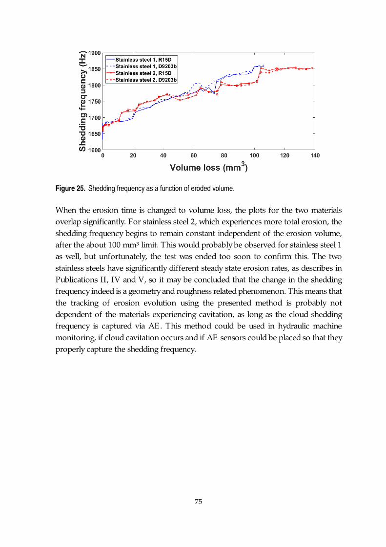
75

Figure 25. Shedding frequency as a function of eroded volume.

When the erosion time is changed to volume loss, the plots for the two materialsoverlap significantly. For stainless steel 2, which experiences more total erosion, theshedding frequency begins to remain constant independent of the erosion volume,after the about 100 mm3 limit. This would probably be observed for stainless steel 1as well, but unfortunately, the test was ended too soon to confirm this. The twostainless steels have significantly different steady state erosion rates, as describes inPublications II, IV and V, so it may be concluded that the change in the sheddingfrequency indeed is a geometry and roughness related phenomenon. This means thatthe tracking of erosion evolution using the presented method is probably notdependent of the materials experiencing cavitation, as long as the cloud sheddingfrequency is captured via AE. This method could be used in hydraulic machinemonitoring, if cloud cavitation occurs and if AE sensors could be placed so that theyproperly capture the shedding frequency.

76

6 CONCLUDING REMARKS

The research questions investigated in this thesis were listed in section 1.2. Thissection aims to evaluate what were the concise answers to these questions and ifthese answers are adequate. The thesis was divided into two main problems:characterizing erosive cavitation and tracking the evolution of cavitation erosion.The attempt to solve both problems included acoustic emission measurements in acavitation tunnel. The used AE data was in the end similar in both approaches; itwas just treated differently. Along with these results, knowledge was gained of theerosion properties of three Francis turbine steels used in runner blades. A secondarygoal was to study if the microstructure-level reasons could be found behind thedifference in erosion rates of two stainless steels that were studied.

The first research question concerned the cavitation erosion resistances of steelsused in runner blades. This was studied through erosion tests in a cavitation tunneland the main results were discussed in Publication II. Three materials were studied:A low-alloy steel and two stainless steels from different turbines. Stainless steel 1,which was from a turbine manufactured in the 1970’s, performed the best from thesethree materials. It also compared well to other steels measured by other authors. Themeasure of cavitation erosion resistance was the steady-state volume loss rate. Thelower this rate, the better the materials resistance. The volume loss rate was chosenover the mass loss rate, as cavitation damage is typically a volume-related problem,as the structural integrity of the machines degrade based on changes in geometry.

The second question of the reason behind the differing rates culminated in themicrostructure analysis of the two studied stainless steels. These two steels had amartensitic microstructure, observed from the optical microscope images inPublication II. Steel 2, which was from a turbine commissioned in 2010’s, and alsoperformed worse that steel 1, seemed to have a larger prior austenite grain size.Optical microscopy did not reveal the accurate grain size, nor any other effects thatmight contribute to the difference. The SEM images from the eroded area inPublication II did not give any insight to this, and they only highlighted that theerosion process is dominated by low-cycle fatigue.

77

The EBSD measurements, presented in Publication V, provided an accurateanswer to this question. Steel 1, while having a prior austenite grain size about halfof that of steel 2, had other advantages as well. It had smaller martensite packet andblock sizes, and most importantly, it had up to 9 vol-% of retained austenite, welldispersed between packets and blocks. This significantly increases the impactstrength, and additionally, it enables an austenite – martensite transformation,contributing to strain-hardening and increased resistance. This transformation wasobserved in the edge regions where cavitation had damaged the specimens.

The third question was about detecting and characterizing individual cavitationimpacts via AE. This method was first discussed in Publication I, where the AEenveloping and peak counting method was presented. The method was furtherdeveloped and the results were compared to pitting measurements in Publication III.The cumulative distributions of both the AE peak voltage values and the cavitationpit diameters, measured through optical microscopy, had a clear correlation. Acorrelation was found between AE peak voltage value and the resulting pit diameter.This allows the estimation of pit distributions through AE measurements in thecavitation tunnel, using parameters that are AE setup and material dependent. Thepit sizes are generally related to the cavitation impact strengths, but this relation wasnot further discussed in this thesis. The presented method was criticized in section3.4, as impacts generated by dropping steel balls on the specimen surface wasobserved to produce varying AE voltages, depending on impact location. This doesnot prove the method false, as the ball drop test might not imitate cavitation impactsproperly, as the specimens were not attached in the cavitation tunnel, nor did theycreate identical loadings compared to cavitation impacts. However, this effect shouldbe further studied to remove doubt.

The fourth research question concentrated on the cavitation erosion tracking viaAE. As the erosion progresses, the specimen surface both hardens and changes ingeometry, through roughness and material loss. The main results were presented inPublication IV. Initially, parameters such as AE event energy and RMS value werestudied as potential indicators of erosion, but they did not provide any clear results.The type of cavitation created in the tunnel is cloud cavitation, which is characterizedby periodical formation and collective collapse of clouds of cavitation bubbles. Thefrequency of these events was assumed to be in the order of several kHz, which wasfar below the AE sensor operation range. However, it was found that the process of

78

demodulation may be used to promote these frequencies in the AE data, as theywere modulated in the high frequency signal. The demodulated frequencies werecompared to those from video analysis and to those from simulations by anotherauthor, thus proving that the AE effectively does capture the shedding phenomenon.It was observed that after the cavitation incubation period, the shedding frequencyincreases with increasing volume loss, until it reaches a quasi-stationary level.

In the author’s opinion, these three results are the key findings of this thesis:

1) Martensitic steels with a small prior austenite grain size, a small packet andblock size and a good fraction of retained austenite dispersed in themicrostructure have a higher cavitation erosion resistance. This provides oneway to rank martensitic steels regarding material choices in hydraulicmachines.

2) The AE enveloping and peak counting method may be used in estimatingcavitation pit diameter distributions.

3) Cloud cavitation shedding frequency increases with increasing volume loss,at least in a simple geometry as in the PREVERO cavitation tunnel, and thechanges in the frequency may be tracked via high frequency AEmeasurements that are demodulated and low-pass filtered beforetransforming them to the spectral domain.

To conclude this thesis, the certainty of these three methods need to be discussed.The results in Publication V are rather well founded, so finding 1 is considered tohave a high certainty and it could be used as a guideline for turbine manufacturersor operators commissioning turbines. The results in Publication III and thestatement in finding 2 are less certain in the author’s opinion, but they might provideinsight in comparing cavitation intensity levels even in hydraulic machines. Themethod seems to perform well in the cavitation tunnel, but additional measurementswith different operation points would be beneficial. Expanding it to hydraulicmachines would require significant work. Finding 3 was considered to have a highcertainty, as the results in Publication IV are consistent and they compare well withother methods. Expanding the method to measure erosion progression in hydraulicmachines would require knowledge of the cavitation types in the machines. Withoutthe periodicity in cloud cavitation, the method has no use. Therefore, in the limited

79

case of cloud cavitation and of transitioning from sheet to cloud cavitation, themethod might prove highly efficient, even in hydraulic machines.

80

REFERENCES

ACHENBACH, J.D. (1975). WAVE PROPAGATION IN ELASTIC SOLIDS, 1ST ED., NORTH

HOLLAND PUBLISHING.

ACOSTA, A.J. & PARKIN, P.R. (1975). CAVITATION INCEPTION - A SELECTIVE REVIEW,JOURNAL OF SHIP RESEARCH, VOL. 19(4), PP. 193-205.

ARABNEJAD, M.H., AMINI, A., BENSOW, R. & FARHAT, M. (2018). EXPERIMENTAL

AND NUMERICAL INVESTIGATION OF THE CAVITATING FLOWS OVER A MODIFIED

NACA0009 FOIL, PROCEEDINGS OF THE 10TH INTERNATIONAL SYMPOSIUM ON

CAVITATION (CAV2018), 2019/02, ASME, NEW YORK, NY, PP. 1-5.

ARNDT, R. (2014). FOREWORD, IN: KIM, K., CHAHINE , G.L., FRANC, J. & KARIMI, A.(ED.), ADVANCED EXPERIMENTAL AND NUMERICAL TECHNIQUES FOR CAVITATION

EROSION PREDICTION, SPRINGER DORDRECHT HEIDELBERG, PP. V-VI.

ARNDT, R., VOIGT, R., SINCLAIR, J., PETER, R. & ANTONIO, F. (1989). CAVITATION

EROSION IN HYDROTURBINES, JOURNAL OF HYDRAULIC ENGINEERING , VOL.115(10), PP. 1297-1315.

ASTM G134-95(2010)E1, STANDARD TEST METHOD FOR EROSION OF SOLID

MATERIALS BY A CAVITATING LIQUID JET (2010).

ASTM G32-10, STANDARD TEST METHOD FOR CAVITATION EROSION USING

VIBRATORY APPARATUS (2010).

AURET, J.G., DAMM, O.F.R.A., WRIGHT, G.J. & ROBINSON, F.P.A. (1993). THE

INFLUENCE OF WATER AIR CONTENT ON CAVITATION EROSION IN DISTILLED WATER,TRIBOLOGY INTERNATIONAL, VOL. 26(6), PP. 431-433.

AVELLAN, F. (2004). INTRODUCTION TO CAVITATION IN HYDRAULIC MACHINERY,THE 6TH INTERNATIONAL CONFERENCE ON HYDRAULIC MACHINERY AND

HYDRODYNAMICS.

81

BATHIAS, C. & PINEAU, A. (2010). LOW-CYCLE FATIGUE , IN: FATIGUE OF MATERIALS

AND STRUCTURES - FUNDAMENTALS, JOHN WILEY & SONS, PP. 113-116.

BERCHICHE , N., FRANC, J.-. & MICHEL, J.-. (2002). A CAVITATION EROSION MODEL

FOR DUCTILE MATERIALS, JOURNAL OF FLUIDS ENGINEERING , VOL. 124(3), PP. 601-606.

BERRY, J.E . (1997A). HIGH FREQUENCY ENVELOPING AND DEMODULATION

TECHNIQUES USING INSTRUMENTS FROM VARIOUS VENDORS, 1ST ED., TECHNICAL

ASSOCIATES OF CHARLOTTE , P.C.

BERRY, J.E . (1997B). TRACKING OF ROLLING ELEMENT BEARING FAILURE STAGES

USING BOTH VIBRATION SIGNATURE ANALYSIS AS WELL AS HIGH FREQUENCY

ENVELOPPING AND DEMODULATION SPECIAL TECHNIQUES, 3RD ED., TECHNICAL

ASSOCIATES OF CHARLOTTE , P.C.

BERTHELOT, M. (1849-1858). SUR QUELQUES PHENOMENES DE DILATION FORCEE

DE LIQUIDES.

BOURDON, P., FARHAT, M., MOSSOBA, Y. & LAVIGNE , P. (1999). HYDRO TURBINE

PROFITABILITY AND CAVITATION EROSION, WATERPOWER '99: HYDRO'S FUTURE :TECHNOLOGY, MARKETS, AND POLICY, 2018/11, PP. 1-10.

BRENNEN, C.E. (1995). CAVITATION AND BUBBLE DYNAMICS, 1ST ED., OXFORD

UNIVERSITY PRESS, OXFORD, UNITED KINGDOM.

BRENNEN, C.E., COLONIUS, Y.C., WANG , A. & PRESTON, A. (2000). CLOUD

CAVITATION PHENOMENA, TWENTY-SECOND SYMPOSIUM ON NAVAL

HYDRODYNAMICS, PP. 239-253.

BRUJAN, E .A., KEEN, G.S., VOGEL, A. & BLAKE , J.R. (2002). THE FINAL STAGE OF

THE COLLAPSE OF A CAVITATION BUBBLE CLOSE TO A RIGID BOUNDARY, PHYSICS OF

FLUIDS, VOL. 14(1), PP. 85.

CARNELLI, D., KARIMI, A. & FRANC, J. (2012). APPLICATION OF SPHERICAL

NANOINDENTATION TO DETERMINE THE PRESSURE OF CAVITATION IMPACTS FROM

PITTING TESTS, JOURNAL OF MATERIALS RESEARCH, VOL. 27(1), PP. 91-99.

82

CARRAT, J., FORTES-PATELLA, R. & FRANC, J. (2017). ASSESSMENT OF CAVITATING

FLOW AGGRESSIVENESS ON A HYDROFOIL: EXPERIMENTAL AND NUMERICAL

APPROACHES, ASME 2017 FLUIDS ENGINEERING DIVISION SUMMER MEETING, PP.V01AT05A013.

CAUPIN, F. & HERBERT, E . (2006). CAVITATION IN WATER: A REVIEW, COMPTES

RENDUS PHYSIQUE , VOL. 7(9–10), PP. 1000-1017.

CHAHINE , G.L., FRANC, J. & KARIMI, A. (2014). CAVITATION AND CAVITATION

EROSION, IN: KIM, K., CHAHINE , G.L., FRANC, J. & KARIMI, A. (ED.), ADVANCED

EXPERIMENTAL AND NUMERICAL TECHNIQUES FOR CAVITATION EROSION

PREDICTION, SPRINGER DORDRECHT HEIDELBERG, PP. 3-20.

CHAHINE , G.L., FRANC, J. & KARIMI, A. (2014). MASS LOSS AND ADVANCED

PERIODS OF EROSION, IN: KIM, K., CHAHINE , G.L., FRANC, J. & KARIMI, A. (ED.),10.1007/978-94-017-8539-6, SPRINGER DORDRECHT HEIDELBERG, PP. 97-121.

CHAHINE , G.L. & KALUMUCK, K.M. (1998). THE INFLUENCE OF STRUCTURAL

DEFORMATION ON WATER JET IMPACT LOADING, JOURNAL OF FLUIDS AND

STRUCTURES, VOL. 12(1), PP. 103-121.

CHEN, T., LIANG, W., ZHANG, M., HUANG , B. & WANG , G. (2018). CAVITATING

FLOWS OF VARYING TEMPERATURE LIQUID NITROGEN IN CONVERGING-DIVERGING NOZZLE , PROCEEDINGS OF THE 10TH INTERNATIONAL SYMPOSIUM ON

CAVITATION (CAV2018), 2019/02, ASME, NEW YORK, NY, PP. 1-6.

CHOI, J.-. & CHAHINE , G.L. (2015). QUANTITATIVE EVALUATION OF EROSIVE

CAVITATION PRESSURE FIELD FROM PITS IN MATERIAL: FACT OR MYTH? 9TH

INTERNATIONAL SYMPOSIUM ON CAVITATION (CAV2015), PP. 1-4.

DEPLANCKE , T., LAME , O., CAVAILLE , J., FIVEL, M., RIONDET, M. & FRANC, J.(2015). OUTSTANDING CAVITATION EROSION RESISTANCE OF ULTRA HIGH

MOLECULAR WEIGHT POLYETHYLENE (UHMWPE) COATINGS, WEAR, VOL. 328–329, PP. 301-308.

DULAR, M. & OSTERMAN, A. (2008). PIT CLUSTERING IN CAVITATION EROSION,WEAR, VOL. 265(5–6), PP. 811-820.

83

DULAR, M., STOFFEL, B. & ŠIROK, B. (2006). DEVELOPMENT OF A CAVITATION

EROSION MODEL, WEAR, VOL. 261(5–6), PP. 642-655.

EDMONDS, D.V., HE , K., RIZZO, F.C., DE COOMAN, B.C., MATLOCK, D.K. & SPEER,J.G. (2006). QUENCHING AND PARTITIONING MARTENSITE—A NOVEL STEEL HEAT

TREATMENT, MATERIALS SCIENCE AND ENGINEERING : A, VOL. 438-440, PP. 25-34.

ESCALER, X., EGUSQUIZA, E ., FARHAT, M., AVELLAN, F. & COUSSIRAT, M. (2006).DETECTION OF CAVITATION IN HYDRAULIC TURBINES, MECHANICAL SYSTEMS AND

SIGNAL PROCESSING, VOL. 20(4), PP. 983-1007.

FARHAT, M. & BOURDON, P. (1998). EXTENDING REPAIR INTE RVALS OF HYDRO

TURBINES BY MITIGATING CAVITATION EROSION, CEA ELECTRICITY '98CONFERENCE AND EXPOSITION.

FORTES PATELLA, R., CHOFFAT, T., REBOUD, J. & ARCHER, A. (2013). MASS LOSS

SIMULATION IN CAVITATION EROSION: FATIGUE CRITERION APPROACH, WEAR, VOL.300(1), PP. 205-215.

FRANC, J. & MICHEL, J. (2005). FUNDAMENTALS OF CAVITATION, 1ST ED., SPRINGER

SCIENCE + BUSINESS MEDIA, INC.

FRANC, J., RIONDET, M., KARIMI, A. & CHAHINE , G.L. (2011). IMPACT LOAD

MEASUREMENTS IN AN EROSIVE CAVITATING FLOW, JOURNAL OF FLUIDS

ENGINEERING , VOL. 133(12), PP. 121301-1-121301-8.

FRANC, J., CHAHINE , G.L. & KARIMI, A. (2014). PITTING AND INCUBATION PERIOD,IN: KIM, K., CHAHINE , G.L., FRANC, J. & KARIMI, A. (ED.), 10.1007/978-94-017-8539-6, SPRINGER DORDRECHT HEIDELBERG, PP. 37-69.

FRANC, J. (2009). INCUBATION TIME AND CAVITATION EROSION RATE OF WORK-HARDENING MATERIALS, JOURNAL OF FLUIDS ENGINEERING, VOL. 131(2), PP.021303.

FRANC, J., RIONDET, M., KARIMI, A. & CHAHINE , G.L. (2012). MATERIAL AND

VELOCITY EFFECTS ON CAVITATION EROSION PITTING , WEAR, VOL. 274–275, PP.248-259.

84

GAVAISES, M., VILLA, F., KOUKOUVINIS, P., MARENGO, M. & FRANC, J. (2015).VISUALISATION AND LES SIMULATION OF CAVITATION CLOUD FORMATION AND

COLLAPSE IN AN AXISYMMETRIC GEOMETRY, INTERNATIONAL JOURNAL OF

MULTIPHASE FLOW, VOL. 68, PP. 14-26.

GNANASKANDAN, A. & MAHESH, K. (2016). LARGE EDDY SIMULATION OF THE

TRANSITION FROM SHEET TO CLOUD CAVITATION OVER A WEDGE , INTERNATIONAL

JOURNAL OF MULTIPHASE FLOW, VOL. 83, PP. 86-102.

GROSSE , C. (2008). INTRODUCTION, IN: GROSSE , C. & OHTSU, M. (ED.), ACOUSTIC

EMISSION TESTING, SPRINGER BERLIN HEIDELBERG, PP. 3-10.

HAMMITT, F.G. (1979). CAVITATION EROSION: THE STATE OF ART AND PREDICTING

CAPABILITY, UNIVERSITY OF MICHIGAN.

HAO, J., ZHANG , M. & HUANG , X. (2017). THE INFLUENCE OF SURFACE ROUGHNESS

ON CLOUD CAVITATION FLOW AROUND HYDROFOILS, ACTA MECHANICA SINICA,VOL. 34(1), PP. 10-21.

HATTORI, S., HIROSE , T. & SUGIYAMA, K. (2010). PREDICTION METHOD FOR

CAVITATION EROSION BASED ON MEASUREMENT OF BUBBLE COLLAPSE IMPACT

LOADS, WEAR, VOL. 269(7–8), PP. 507-514.

HATTORI, S. & ISHIKURA, R. (2010). REVISION OF CAVITATION EROSION DATABASE

AND ANALYSIS OF STAINLESS STEEL DATA, WEAR, VOL. 268(1–2), PP. 109-116.

HATTORI, S., ISHIKURA, R. & ZHANG, Q. (2004). CONSTRUCTION OF DATABASE ON

CAVITATION EROSION AND ANALYSES OF CARBON STEEL DATA, WEAR, VOL. 257(9–10), PP. 1022-1029.

HATTORI, S. & KITAGAWA, T. (2010). ANALYSIS OF CAVITATION EROSION

RESISTANCE OF CAST IRON AND NONFERROUS METALS BASED ON DATABASE AND

COMPARISON WITH CARBON STEEL DATA, WEAR, VOL. 269(5–6), PP. 443-448.

HATTORI, S. & NAKAO, E . (2002). CAVITATION EROSION MECHANISMS AND

QUANTITATIVE EVALUATION BASED ON EROSION PARTICLES, WEAR, VOL. 249(10–11), PP. 839-845.

85

HE , Y. & SHEN, Z. (2012). EXPERIMENTAL RESEARCH ON CAVITATION EROSION

DETECTION BASED ON ACOUSTIC EMISSION TECHNIQUE , 30TH EUROPEAN

CONFERENCE ON ACOUSTIC EMISSION TESTING & 7TH INTERNATIONAL

CONFERENCE ON ACOUSTIC EMISSION, PP. 1-8.

HEYES, D.M. (2008). LIQUIDS AT POSITIVE AND NEGATIVE PRESSURE , PHYSICA

STATUS SOLIDI (B), VOL. 245(3), PP. 530-538.

HOLROYD, T. (2000). ACOUSTIC EMISSION AND ULTRASONICS HANDBOOK

(COXMOOR'S MACHINE & SYSTEM CONDITION MONITORING), COXMOOR

PUBLISHING CO., MORETON-IN-MARSH, UNITED KINGDOM.

HSIAO, C., JAYAPRAKASH, A., KAPAHI, A., CHOI, J. & CHAHINE , G.L. (2014).MODELLING OF MATERIAL PITTING FROM CAVITATION BUBBLE COLLAPSE

, JOURNAL OF FLUID MECHANICS, VOL. 755, PP. 142-175.

HSIAO, C. & CHAHINE , G.L. (2013). DEVELOPMENT OF COMPRESSIBLE-INCOMPRESSIBLE LINK TO EFFICIENTLY MODEL BUBBLE DYNAMICS NEAR

FLOATING BODY FLOW STAGE FLUID CODE INTERFACE STRUCTURE CODE , BETEQ

2013 XIV INTE RNATIONAL CONFERENCE ON BOUNDARY ELEMENT & MESHLESS

TECHNIQUIES.

HSIAO, C., MA, J. & CHAHINE , G.L. (2017). MULTISCALE TOW-PHASE FLOW

MODE LING OF SHEET AND CLOUD CAVITATION, INTERNATIONAL JOURNAL OF

MULTIPHASE FLOW, VOL. 90, PP. 102-117.

HUJER, J., CARRAT, J., MÜLLER, M. & RIONDET, M. (2015). IMPACT LOAD

MEASUREMENTS WITH A PVDF PRESSURE SENSOR IN AN EROSIVE CAVITATING FLOW,JOURNAL OF PHYSICS: CONFERENCE SERIES, VOL. 656(012051), PP. 1-4.

HUJER, J. & MULLER, M. (2018). SPATIAL DISTRIBUTION OF THE CAVITATION

AGGRESSIVENESS IN A HIGH SPEED CAVITATION TUNNEL, 10TH INTE RNATIONAL

SYMPOSIUM ON CAVITATION (CAV2018), PP. 939-942.

INABA, H. (2016). AE SENSOR (AE TRANSDUCER), IN: PRACTICAL ACOUSTIC

EMISSION TESTING, THE JAPANESE SOCIETY FOR NON-DESTRUCTIVE INSPECTION,PP. 35-45.

86

KAISER, J. (1950). UNTERSUCHUNGEN ÜBER DAS AUFTRETEN VON GERÄUSCHEN

BEIM ZUGVERSUCH (A STUDY OF ACOUSTIC PHENOMENA IN TENSILE TESTS),

DOCTORAL THESIS, TECHNISCHE HOCHSCHULE MÜNCHEN, GERMANY.

KANG , C., LIU, H. & SOYAMA, H. (2018). ESTIMATION OF AGGRESSIVE INTENSITY OF

A CAVITATING JET WITH MULTIPLE EXPERIMENTAL METHODS, WEAR, VOL. 394-395,PP. 176-186.

KARIMI, A. (1987). CAVITATION EROSION OF A DUPLEX STAINLESS STEEL,MATERIALS SCIENCE AND ENGINEERING, VOL. 86, PP. 191-203.

KARIMI, A. & LEO, W.R. (1987). PHENOMENOLOGICAL MODEL FOR CAVITATION

EROSION RATE COMPUTATION, MATERIALS SCIENCE AND ENGINEERING, VOL. 95,PP. 1-14.

KEIL, T., PELZ, P.F. & BUTTENBENDER, J. (2012). ON THE TRANSITION FROM SHEET

TO CLOUD CAVITATION, PROCEEDINGS OF THE 8TH INTERNATIONAL SYMPOSIUM

ON CAVITATION.

KENDRICK, H., LIGHT, M.S. & CACCESE , V. (2005). DEVELOPMENT OF A

CAVITATION EROSION RESISTANT ADVANCE D MATERIAL SYSTEM.

KIM, K.H., CHAHINE , G., FRANC, J.P. & KARIMI, A. (2014). ADVANCED

EXPERIMENTAL AND NUMERICAL TECHNIQUES FOR CAVITATION EROSION

PREDICTION, 1ST ED., SPRINGER, 399 P.

KIM, H.J., KIM, Y.H. & MORRIS, J.J.W. (1998). THERMAL MECHANISMS OF GRAIN

AND PACKET REFINEMENT IN A LATH MARTENSITIC STEEL, ISIJ INTE RNATIONAL,VOL. 38(11), PP. 1277-1285.

KNAPP, R.T., DAILY, J.W. & HAMMITT, F.G. (1970). CAVITATION, MCGRAW-HILL,NEW YORK, 578 P.

KWOK, C.T., CHENG , F.T. & MAN, H.C. (2006). CAVITATION EROSION AND

CORROSION BEHAVIORS OF LASER-ALUMINIZED MILD STEEL, SURFACE AND

COATINGS TECHNOLOGY, VOL. 200(11), PP. 3544-3552.

87

LOOK, A., KIRSCHNER, O., RIEDELBAUCH, S. & NECKER, J. (2018). DETECTION AND

LEVEL ESTIMATION OF CAVITATION IN HYDRAULIC TURBINES WITH

CONVOLUTIONAL NEURAL NETWORKS, THE 10TH INTE RNATIONAL SYMPOSIUM ON

CAVITATION (CAV2018), PP. 1-4.

MARPLE JR, L. (1999). COMPUTING THE DISCRETE-TIME "ANALYTIC" SIGNAL VIA

FFT, IEEE TRANSACTIONS ON SIGNAL PROCESSING, VOL. 47, PP. 2600-2603.

MILLS, A.F. (1999). BASIC HEAT & MASS TRANSFER, 2ND ED., PRENTICE HALL.

NISHIMURA, S., TAKAKUWA, O. & SOYAMA, H. (2014). EFFECT OF NOZZLE

GEOMETRY ON AGGRESSIVITY OF CAVITATING JET FOR CAVITATION EROSION TEST

AND APPLICATIONS, IN: KIM, K., CHAHINE , G., FRANC, J. & KARIMI, A. (ED.),ADVANCED EXPERIMENTAL AND NUMERICAL TECHNIQUES FOR CAVITATION

EROSION PREDICTION, SPRINGER NETHERLANDS, DORDRECHT, PP. 283-302.

NYYSSÖNEN, T., ISAKOV, M., PEURA, P. & KUOKKALA, V. (2016). ITERATIVE

DETERMINATION OF THE ORIENTATION RELATIONSHIP BETWEEN AUSTENITE AND

MARTENSITE FROM A LARGE AMOUNT OF GRAIN PAIR MISORIENTATIONS,METALLURGICAL AND MATERIALS TRANSACTIONS A, VOL. 47(6), PP. 2587-2590.

NYYSSÖNEN, T. (2017). QUENCHING AND PARTITIONING OF HIGH-ALUMINUM

STEELS; QUENCHING AND PARTITIONING OF HIGH-ALUMINUM STEELS, TAMPERE

UNIVERSITY OF TECHNOLOGY.

OBRESCHKOW, D. (2012). ANALYTICAL APPROXIMATIONS FOR THE COLLAPSE OF AN

EMPTY SPHERICAL BUBBLE , PHYSICAL REVIEW.E , STATISTICAL, NONLINEAR, AND

SOFT MATTER PHYSICS, VOL. 85(6), PP. 066303.

OHTSU, M., ENOKI, M., MIZUTANI, Y. & SHIGEISHI, M. (2016). PRINCIPLES OF THE

ACOUSTIC EMISSION (AE) METHOD AND SIGNAL PROCESSING, IN: PRACTICAL

ACOUSTIC EMISSION TESTING, THE JAPANESE SOCIETY FOR NON-DESTRUCTIVE

INSPECTION, PP. 5-35.

OHTSU, M. (2008). SENSOR AND INSTRUMENT, IN: GROSSE , C. & OHTSU, M. (ED.),ACOUSTIC EMISSION TESTING, SPRINGER BERLIN HEIDELBERG, HEIDELBERG,GERMANY, PP. 19-40.

88

PELZ, P., KEIL, T. & GROß, T. (2017). THE TRANSITION FROM SHEET TO CLOUD

CAVITATION, JOURNAL OF FLUID MECHANICS, VOL. 817, PP. 439-454.

PELZ, P., KEIL, T. & LUDWIG, G. (2014). ON THE KINEMATICS OF SHEET AND

CLOUD CAVITATION AND RELATED EROSION, FLUID MECHANICS AND ITS

APPLICATIONS, VOL. 106, PP. 221-237.

PETERS, A., LANTERMANN, U. & EL MOCTAR, O. (2015). NUMERICAL MODELLING

AND PREDICTION OF EROSION INDUCED BY HYDRODYNAMIC CAVITATION,JOURNAL OF PHYSICS: CONFERENCE SERIES, VOL. 656, PP. 012054.

PLESSET, M.S. (1949). THE DYNAMICS OF CAVITATION, JOURNAL OF APPLIED

MECHANICS, VOL. 16, PP. 277-282.

PLESSET, M.S. (1970). EFFECT OF DISSOLVED GASES ON CAVITATION IN LIQUIDS.

PLESSET, M.S. & CHAPMAN, R.P. (1971). COLLAPSE OF AN INITIALLY SPHERICAL

VAPOUR CAVITY IN THE NEIGHBOURHOOD OF A SOLID BOUNDARY, JOURNAL OF

FLUID MECHANICS, VOL. 47(2), PP. 283-290.

PLESSET, M.S. & PROSPERETTI, A. (1977). BUBBLE DYNAMICS AND CAVITATION,ANNUAL REVIEW OF FLUID MECHANICS, VOL. 9, PP. 145-185.

PREVERO 2018. THE PREVERO CAVITATION EROSION TUNNEL, WEB PAGE .AVAILABLE (ACCESSED 25/10/2019):HTTP://WEB.ARCHIVE .ORG/WEB/20180327065723/HTTP://WWW.LEGI.GRENOBLE

-INP.FR/WEB/SPIP.PHP?ARTICLE1265&LANG= FR.

PÖHL, F., MOTTYLL, S., SKODA, R. & HUTH, S. (2015). EVALUATION OF CAVITATION-INDUCED PRESSURE LOADS APPLIED TO MATERIAL SURFACES BY FINITE-ELEMENT-ASSISTED PIT ANALYSIS AND NUMERICAL INVESTIGATION OF THE ELASTO-PLASTIC

DEFORMATION OF METALLIC MATERIALS, WEAR, VOL. 330–331, PP. 618-628.

RAYLEIGH, L. (1917). PRESSURE DEVELOPED IN A LIQUID DURING THE COLLAPSE

OF A SPHERICAL CAVITY, PHILOSOPHICAL MAGAZINE , VOL. 34, PP. 504-507.

ROY, S.C. (2015). MODELING AND ANALYSIS OF MATERIAL BEHAVIOR DURING

CAVITATION EROSION, DOCTORAL THESIS, UNIVERSITÉ GRENOBLE ALPES, FRANCE .

89

ROY, S.C., FRANC, J. & FIVEL, M. (2015). CAVITATION EROSION: USING THE

MATE RIAL AS A PRESSURE SENSOR, JOURNAL OF APPLIED PHYSICS, VOL. 118(16), PP.164905.

ROY, S.C., FRANC, J., RANC, N. & FIVEL, M. (2015). DETERMINATION OF

CAVITATION LOAD SPECTRA—PART 2: DYNAMIC FINITE ELEMENT APPROACH,WEAR, VOL. 344-345, PP. 120-129.

RYL, J., DAROWICKI, K. & SLEPSKI, P. (2011). EVALUATION OF CAVITATION

EROSION–CORROSION DEGRADATION OF MILD STEEL BY MEANS OF DYNAMIC

IMPEDANCE SPECTROSCOPY IN GALVANOSTATIC MODE , CORROSION SCIENCE , VOL.53(5), PP. 1873-1879.

SCHMIDT, H., KIRSCHNER, O. & RIEDELBAUCH, S. (2015). CAVITATION

MEASUREMENTS ON A PUMP-TURBINE MODEL, JOURNAL OF PHYSICS: CONFERENCE

SERIES, VOL. 656(012051), PP. 1-4.

SCHMIDT, H., KIRSCHNER, O., RIEDELBAUCH, S., NECKER, J., KOPF, E ., RIEG , M.,ARANTES, G., WESSIAK, M. & MAYRHUBER, J. (2014). INFLUENCE OF THE VIBRO-ACOUSTIC SENSOR POSITION ON CAVITATION DETECTION IN A KAPLAN TURBINE ,IOP CONFERENCE SERIES: EARTH AND ENVIRONMENTAL SCIENCE , VOL.22(052006), PP. 1-9.

SCHWARZER, R., FIELD, D., ADAMS, B., KUMAR, M. & SCHWARTZ, A. (2009).PRESENT STATE OF ELECTRON BACKSCATTER DIFFRACTION AND PROSPECTIVE

DEVELOPMENTS, IN: SCHWARTZ, A., KUMAR, M., ADAMS, B. & FIELD, D. (ED.),ELECTRON BACKSCATTER DIFFRACTION IN MATERIALS SCIENCE , 2ND ED.,SPRINGER SCIENCE + BUSINESS MEDIA, PP. 1-20.

SOYAMA, H. (2013). EFFECT OF NOZZLE GEOMETRY ON A STANDARD CAVITATION

EROSION TEST USING A CAVITATING JET, WEAR, VOL. 297(1–2), PP. 895-902.

SOYAMA, H. & FUTAKAWA, M. (2004). ESTIMATION OF INCUBATION TIME OF

CAVITATION EROSION FOR VARIOUS CAVITATING CONDITIONS, TRIBOLOGY

LETTERS, VOL. 17(1), PP. 27-30.

90

STELLER, J., KRELLA, A., KORONOWICZ, J. & JANICKI, W. (2005). TOWARDS

QUANTITATIVE ASSESSMENT OF MATERIAL RESISTANCE TO CAVITATION EROSION,WEAR, VOL. 258(1–4), PP. 604-613.

STUTZ, B. (2003). INFLUENCE OF ROUGHNESS ON THE TWO-PHASE FLOW

STRUCTURE OF SHEET CAVITATION, JOURNAL OF FLUIDS ENGINEERING , VOL.125(4), PP. 652-659.

VAN RIJSBERGEN, M., FOETH, E ., FITZSIMMONS, P. & BOORSMA, A. (2012). HIGH-SPEED VIDEO OBSERVATIONS AND ACOUSTIC-IMPACT MEASUREMENTS ON A

NACA 0015 FOIL, 8TH INTE RNATIONAL SYMPOSIUM ON CAVITATION (CAV 2012),01/01, PP. 958-964.

YLÖNEN, M. (2016). CAVITATION EROSION CHARACTERIZATION OF FRANCIS

TURBINE RUNNER BLADE MATERIAL, MASTER OF SCIENCE THESIS, TAMPERE

UNIVERSITY OF TECHNOLOGY, FINLAND.

YOUNG, R.F. (1989). CAVITATION, 1ST ED., MCGRAW-HILL.

ZAVALETA GUTIÉRREZ, N., LUPPO, M.I., DANON, C.A., TODA-CARABALLO, I.,CAPDEVILA, C. & GARCÍA, D.A. (2013). HETEROGENEOUS AUSTENITE GRAIN

GROWTH IN MARTENSITIC 9CR STEEL: COUPLED INFLUENCE OF INITIAL

METALLURGICAL STATE AND HEATING RATE , MATERIALS SCIENCE AND

TECHNOLOGY, VOL. 29(10), PP. 1254-1266.

ZHANG , S., DUNCAN, J.H. & CHAHINE , G.L. (1994). THE BEHAVIOR OF A

CAVITATION BUBBLE NEAR A RIGID WALL, FLUID MECHANICS AND ITS

APPLICATIONS, VOL. 23, PP. 429-436.

ZHANG , S., DUNCAN, J.H. & CHAHINE , G.L. (1993). THE FINAL STAGE OF THE

COLLAPSE OF A CAVITATION BUBBLE NEAR A RIGID WALL, JOURNAL OF FLUID

MECHANICS, VOL. 257, PP. 147-181.

ZHOU, Y. & HAMMITT, F.G. (1983). CAVITATION EROSION INCUBATION PERIOD,WEAR, VOL. 86, PP. 299-313.

91

PUBLICATIONS

92

PUBLICATIONI

Cavitation Bubble Collapse Monitoring by Acoustic E mission in LaboratoryTesting

Ylönen, Markku., Saarenrinne, Pentti., Miettinen, Juha., Franc, Jean-Pierre. & Fivel,Marc.

Proceedings of the 10th Symposium on Cavitation (CAV2018). 2018, p. 179-184. 05037(https://doi.org/10.1115/1.861851_ch35)

Publication reprinted with kind permission by The American Society of MechanicalE ngineers.

179

[6] Kim, W., Kim, T. H., Choi, J., Kim, H. Y. (2009). Mechanism of particle removal by megasonic waves. Appl. Phys. Lett. 94, 081908. [7] Karri, B., Gonzalez-A., S. R., Loke, Y. C., O’Shea, S. J., Klaseboer, E., Khoo, B. C., Ohl, C-D. (2012). High-speed jetting and spray formation from bubble collapse. Phys. Rev. E 85, 015303. [8] Tagawa, Y., Oudalov, N., El Ghalbzouri, A., Sun, C., Lohse, D. (2013). Needle-free injection into skin and soft matter with highly focused microjets. Lab Chip 13, 1357–1363. [9] Gonzalez-Avila, S. R., Song, C., Ohl, C-D. (2015). Fast transient microjets induced by hemispherical cavitation bubbles. J. Fluid Mech., 767, 31-51.

*Corresponding Author, Markku Ylönen: markku.ylonen@tut.fi

Cavitation Bubble Collapse Monitoring by Acoustic Emission in Laboratory Testing1Markku Ylönen*; 1Pentti Saarenrinne; 1Juha Miettinen; 2Jean-Pierre Franc; 3Marc Fivel

1Tampere University of Technology, 33720 Tampere, Finland; 2Université Grenoble Alpes, CNRS, Grenoble INP, LEGI, 38000Grenoble, France; 3Université Grenoble Alpes, CNRS, Grenoble INP, SIMAP, 38000 Grenoble, France

AbstractIn order to investigate the potential of the acoustic emission technique in predicting cavitation erosion, laboratory tests wereconducted in a high-speed cavitation tunnel. One face of a cylindrical stainless steel sample was subjected to an annular cavitationfield created by the PREVERO cavitation tunnel [1]. Acoustic emission was measured from the back surface of the sample in orderto detect impacts caused by cavitation bubble or cloud collapses. Cavitation aggressiveness was varied by changing the operatingparameters of the cavitation tunnel. Two different operating points were compared. Collapsing cavitation bubbles lead to impactstowards the sample surface and they induce elastic waves in the material. A resonance type acoustic emission sensor with aresonance frequency of 160 kHz captured these waves during the cavitation tests. The acoustic emission waveform was measuredwith a sampling frequency of 5 MHz. The sensor was mounted behind the sample using a wave-guide that maintained a transferpath for the elastic waves to travel from the impacted surface to the sensor. The elastic waves reaching the sensor were observedas distinguishable bursts in the acoustic emission waveform. Acoustic emission from cavitation impacts was estimated to be about100 times stronger than acoustic emission from other sources, such as hydrodynamic events or machine vibration. This means thatthe signal was almost entirely induced by cavitation. The bursts contain multiple reflections that attenuate in time and that have afrequency content corresponding to the sensor frequency response. The bursts attenuate quickly enough not to overlap, as thecavitation events occur with a large enough temporal separation. The hypothesis in this study is that the maximum amplitude ofthe acoustic emission event voltage correlates with the strength of the cavitation bubble collapse impacting the surface. Voltagepeak value counting was applied to the acoustic emission waveform data. As the bursts contain multiple amplitude peaks due tosensor resonance, an envelope function was fitted to the waveform for peak counting. Using this method, each counted voltagepeak value is expected to correspond to a single cavitation impact event. The pulse distribution shows an exponential decrease witha decreasing voltage peak value rate as the peak voltage increases. This compares well with earlier studies, such as [2] and [3],where an exponential distribution of bubble collapse amplitudes was found. The results of this study prove acoustic emission as adirect and non-intrusive method that can be used to monitor cavitation impacts from outside of the cavitation field.

Keywords: cavitation impact detection; acoustic emission; cavitation intensity;

Introduction

The impact load induced by a cavitation bubble collapsing near a solid boundary has been studied by multiple methods,both experimental and computational. In a cavitating flow, the impact load determines material damage in a boundarycaused by a single bubble or bubble cloud collapse. Another important factor in material damage is the impactfrequency, as cavitation erosion tends to be a cumulative process [4-6]. The impact distribution that combines theimpact frequency and amplitude of the cavitation impact loads is essential in determining the cavitation intensity of aflow.

Cavitation impact loads have been measured by various methods. Franc et al. [2] measured the impact loads in thePREVERO cavitation tunnel with conventional pressure sensors flush-mounted in the cavitation closure region. Hujeret al. [3] used PVDF pressure sensors, also flush-mounted in the same tunnel. Both of them observed exponentialimpact distributions. Hattori et al. [7] studied the impact pressures in an ASTM G-32 vibratory device and Okada etal. [8] used the same device to calibrate pressure sensors for a Venturi nozzle test. In the vibratory test, the impactdistribution also follows an exponential law. Franc et al. [9] also observed the pits formed by cavitation impacts andthey observed an exponential distribution in the pit size distribution. The pit shape factor or the ratio between pit depthand pit diameter increases with increasing cavitation intensity, meaning that larger impacts lead to deeper pits [10].

Several authors have studied acoustic emission (AE) as a method to detect and characterize cavitation and cavitationerosion. Boorsma and Fitzsimmons [11] created a cavitation monitoring method for ship rudders and propellers.Yongyong and Zaiyang [12] connected the AE-event energy to mass loss in an ASTM-G32 vibratory cavitationapparatus. Schmidt et al [13; 14] worked on a cavitation detection system based in AE on a prototype Kaplan turbine.They discovered that with properly placed sensors, cavitation leads to increase in AE root mean squared voltage value,event energy and fluctuation of both. Van Rijsbergen et al. [15] found that acoustic emission sensors in direct contact

10th International Symposium on Cavitation - CAV2018

Baltimore, Maryland, USA, May 14 – 16, 2018

CAV18-05037

Downloaded From: http://ebooks.asmedigitalcollection.asme.org on 01/14/2019 Terms of Use: http://www.asme.org/about-asme/terms-of-use

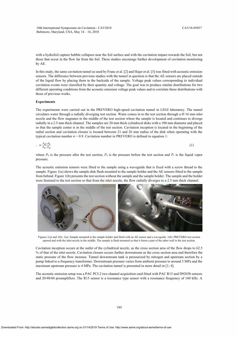
180

with a hydrofoil capture bubble collapses near the foil surface and with the cavitation impact towards the foil, but notthose that occur in the flow far from the foil. These studies encourage further development of cavitation monitoringby AE.

In this study, the same cavitation tunnel as used by Franc et al. [2] and Hujer et al. [3] was fitted with acoustic emissionsensors. The difference between previous studies with the tunnel in question is that the AE sensors are placed outsideof the liquid flow by placing them in the backside of the sample. Voltage peak values corresponding to individualcavitation events were classified by their quantity and voltage. The goal was to produce similar distributions for twodifferent operating conditions from the acoustic emission voltage peak values and to correlate these distributions withthose of previous works.

Experiments

The experiments were carried out in the PREVERO high-speed cavitation tunnel in LEGI laboratory. The tunnelcirculates water through a radially diverging test section. Water comes in to the test section through a Ø 16 mm inletnozzle and the flow stagnates in the middle of the test section where the sample is located and continues to divergeradially in a 2.5 mm thick channel. The samples are 20 mm thick cylindrical disks with a 100 mm diameter and placedso that the sample center is in the middle of the test section. Cavitation inception is located in the beginning of theradial section and cavitation closure is located between 21 and 26 mm radius of the disk when operating with thetypical cavitation number σ = 0.9. Cavitation number in PREVERO is defined in equation 1:. = (1)

where Pd is the pressure after the test section, Pu is the pressure before the test section and Pv is the liquid vaporpressure.

The acoustic emission sensors were fitted to the sample using a waveguide that is fixed with a screw thread to thesample. Figure 1(a) shows the sample disk flush mounted to the sample holder and the AE sensors fitted to the samplefrom behind. Figure 1(b) presents the test section without the sample and the sample holder. The sample and the holderwere fastened to the test section so that from the inlet nozzle, the flow radially diverges to a 2.5 mm thick channel.

Figures 1(a) and 1(b). 1(a): Sample mounted to the sample holder and fitted with an AE sensor and a waveguide. 1(b): PREVERO test sectionopened and with the inlet nozzle in the middle. The sample is flush mounted so that it forms a part of the other wall in the test section.

Cavitation inception occurs at the outlet of the cylindrical nozzle, as the cross section area of the flow drops to 62.5% of that of the inlet nozzle. Cavitation closure occurs further downstream as the cross section area and therefore thestatic pressure of the flow increase. Tunnel downstream tank is pressurized by nitrogen and upstream section by apump linked to a frequency transformer. Downstream pressure varies from ambient pressure to around 3 MPa and themaximum upstream pressure is 4 MPa. The cavitation tunnel is presented in more detail in [1; 4].

The acoustic emission setup was a PAC PCI-2 two channel acquisition card fitted with PAC R15 and D9203b sensorsand 20/40/60 preamplifiers. The R15 sensor is a resonance type sensor with a resonance frequency of 160 kHz. A

10th International Symposium on Cavitation - CAV2018

Baltimore, Maryland, USA, May 14 – 16, 2018

CAV18-05037

band-pass filter from 100 kHz to 400 kHz was used. The D9203b sensor is a broadband sensor with a frequency rangefrom 100 kHz to 900 kHz. In this study, only the data acquired with the R15 sensor were analyzed. The samples weremade of a stainless steel used in Francis turbines and the waveguides were made of steel.

In this study, two samples were mirror polished with successive diamond pastes and a colloidal silica suspension. Onesample was subjected to cavitation erosion for 2 minutes with a 4 MPa upstream pressure and the other for 6 minuteswith a 2 MPa upstream pressure. The 4 MPa and the 2 MPa upstream pressures correspond to 89.4 m/s and 63.2 m/scavity reference velocities, respectively. Cavity reference velocity is defined as the velocity in the test section wherepressure is assumed as vapor pressure. A more detailed explanation of cavity reference velocity is in [4]. Pits with thistype of exposure covered roughly 10 % of the surface of the cavitation closure area. The cavitation impacts were thusassumed to be hitting virgin material most of the time. Acoustic emission waveforms were acquired with a samplingfrequency of 5 MHz for the full duration of the tests.

Peak value distribution by an envelope function

Impacts in the cavitation sample surface were observed in the AE waveform as quickly rising voltage peaks thatdiminish exponentially. The AE waveforms were analyzed in time-voltage space. Wave propagation in the sampleand the waveguide may affect the waveforms, but this effect is not considered in detail in this study. The frequencycontent of each cavitation burst or AE-event resembles that of the sensor frequency response, meaning that the impactsprovoke sensor resonance. This means that the events are mostly short duration impacts compared to the sensor timescales. It is assumed that each voltage peak value in the waveform, with its resonance effects, corresponds to onecavitation impact towards the sample surface. The length of a cavitation bubble collapse is in the range of somemicroseconds up to some tens of microseconds [2; 16]. Through waveform observations, impact overlapping seemsnot to be significant.

With the assumption that each measured maximum in the voltage peak value corresponds to a single cavitation event,there is a need to filter out the sensor resonance effects when peak counting is applied. In most cases in this study, theacoustic emission waveform contains more or less isolated events with breaks between them. Each event has a distinctmaximum or sometimes two or more maximums. To negate the resonance effects, an envelope function is fitted to thewaveform. As the signal is approximately symmetric around zero volts, the absolute value of the signal is calculated.After this, the envelope function was fitted to the waveform. The envelope was calculated by spline interpolation overlocal maximums. The minimum distance between local peaks was set to 16 µs, which is about five times the distancebetween peaks resulting from sensor resonance. This value was found to be suitable through trial and error method.Figure 2 presents a typical AE waveform sample fitted with an envelope function.

Downloaded From: http://ebooks.asmedigitalcollection.asme.org on 01/14/2019 Terms of Use: http://www.asme.org/about-asme/terms-of-use

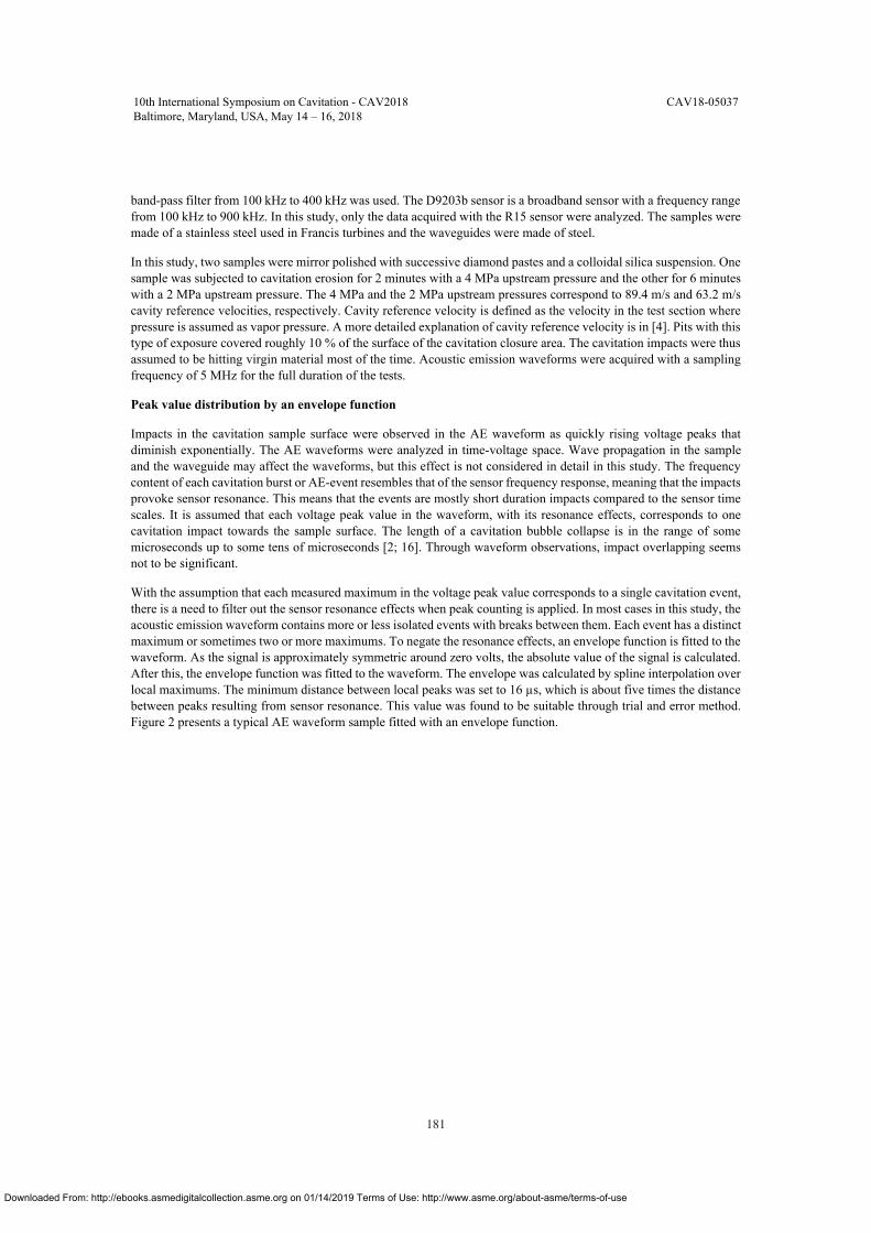
181

with a hydrofoil capture bubble collapses near the foil surface and with the cavitation impact towards the foil, but notthose that occur in the flow far from the foil. These studies encourage further development of cavitation monitoringby AE.

In this study, the same cavitation tunnel as used by Franc et al. [2] and Hujer et al. [3] was fitted with acoustic emissionsensors. The difference between previous studies with the tunnel in question is that the AE sensors are placed outsideof the liquid flow by placing them in the backside of the sample. Voltage peak values corresponding to individualcavitation events were classified by their quantity and voltage. The goal was to produce similar distributions for twodifferent operating conditions from the acoustic emission voltage peak values and to correlate these distributions withthose of previous works.

Experiments

The experiments were carried out in the PREVERO high-speed cavitation tunnel in LEGI laboratory. The tunnelcirculates water through a radially diverging test section. Water comes in to the test section through a Ø 16 mm inletnozzle and the flow stagnates in the middle of the test section where the sample is located and continues to divergeradially in a 2.5 mm thick channel. The samples are 20 mm thick cylindrical disks with a 100 mm diameter and placedso that the sample center is in the middle of the test section. Cavitation inception is located in the beginning of theradial section and cavitation closure is located between 21 and 26 mm radius of the disk when operating with thetypical cavitation number σ = 0.9. Cavitation number in PREVERO is defined in equation 1:. = (1)

where Pd is the pressure after the test section, Pu is the pressure before the test section and Pv is the liquid vaporpressure.

The acoustic emission sensors were fitted to the sample using a waveguide that is fixed with a screw thread to thesample. Figure 1(a) shows the sample disk flush mounted to the sample holder and the AE sensors fitted to the samplefrom behind. Figure 1(b) presents the test section without the sample and the sample holder. The sample and the holderwere fastened to the test section so that from the inlet nozzle, the flow radially diverges to a 2.5 mm thick channel.

Figures 1(a) and 1(b). 1(a): Sample mounted to the sample holder and fitted with an AE sensor and a waveguide. 1(b): PREVERO test sectionopened and with the inlet nozzle in the middle. The sample is flush mounted so that it forms a part of the other wall in the test section.

Cavitation inception occurs at the outlet of the cylindrical nozzle, as the cross section area of the flow drops to 62.5% of that of the inlet nozzle. Cavitation closure occurs further downstream as the cross section area and therefore thestatic pressure of the flow increase. Tunnel downstream tank is pressurized by nitrogen and upstream section by apump linked to a frequency transformer. Downstream pressure varies from ambient pressure to around 3 MPa and themaximum upstream pressure is 4 MPa. The cavitation tunnel is presented in more detail in [1; 4].

The acoustic emission setup was a PAC PCI-2 two channel acquisition card fitted with PAC R15 and D9203b sensorsand 20/40/60 preamplifiers. The R15 sensor is a resonance type sensor with a resonance frequency of 160 kHz. A

band-pass filter from 100 kHz to 400 kHz was used. The D9203b sensor is a broadband sensor with a frequency rangefrom 100 kHz to 900 kHz. In this study, only the data acquired with the R15 sensor were analyzed. The samples weremade of a stainless steel used in Francis turbines and the waveguides were made of steel.

In this study, two samples were mirror polished with successive diamond pastes and a colloidal silica suspension. Onesample was subjected to cavitation erosion for 2 minutes with a 4 MPa upstream pressure and the other for 6 minuteswith a 2 MPa upstream pressure. The 4 MPa and the 2 MPa upstream pressures correspond to 89.4 m/s and 63.2 m/scavity reference velocities, respectively. Cavity reference velocity is defined as the velocity in the test section wherepressure is assumed as vapor pressure. A more detailed explanation of cavity reference velocity is in [4]. Pits with thistype of exposure covered roughly 10 % of the surface of the cavitation closure area. The cavitation impacts were thusassumed to be hitting virgin material most of the time. Acoustic emission waveforms were acquired with a samplingfrequency of 5 MHz for the full duration of the tests.

Peak value distribution by an envelope function

Impacts in the cavitation sample surface were observed in the AE waveform as quickly rising voltage peaks thatdiminish exponentially. The AE waveforms were analyzed in time-voltage space. Wave propagation in the sampleand the waveguide may affect the waveforms, but this effect is not considered in detail in this study. The frequencycontent of each cavitation burst or AE-event resembles that of the sensor frequency response, meaning that the impactsprovoke sensor resonance. This means that the events are mostly short duration impacts compared to the sensor timescales. It is assumed that each voltage peak value in the waveform, with its resonance effects, corresponds to onecavitation impact towards the sample surface. The length of a cavitation bubble collapse is in the range of somemicroseconds up to some tens of microseconds [2; 16]. Through waveform observations, impact overlapping seemsnot to be significant.

With the assumption that each measured maximum in the voltage peak value corresponds to a single cavitation event,there is a need to filter out the sensor resonance effects when peak counting is applied. In most cases in this study, theacoustic emission waveform contains more or less isolated events with breaks between them. Each event has a distinctmaximum or sometimes two or more maximums. To negate the resonance effects, an envelope function is fitted to thewaveform. As the signal is approximately symmetric around zero volts, the absolute value of the signal is calculated.After this, the envelope function was fitted to the waveform. The envelope was calculated by spline interpolation overlocal maximums. The minimum distance between local peaks was set to 16 µs, which is about five times the distancebetween peaks resulting from sensor resonance. This value was found to be suitable through trial and error method.Figure 2 presents a typical AE waveform sample fitted with an envelope function.

10th International Symposium on Cavitation - CAV2018

Baltimore, Maryland, USA, May 14 – 16, 2018

CAV18-05037

Downloaded From: http://ebooks.asmedigitalcollection.asme.org on 01/14/2019 Terms of Use: http://www.asme.org/about-asme/terms-of-use

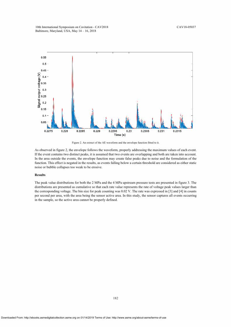
182

Figure 2. An extract of the AE waveform and the envelope function fitted to it.

As observed in figure 2, the envelope follows the waveform, properly addressing the maximum values of each event.If the event contains two distinct peaks, it is assumed that two events are overlapping and both are taken into account.In the area outside the events, the envelope function may create false peaks due to noise and the formulation of thefunction. This effect is negated in the results, as events falling below a certain threshold are considered as either staticnoise or bubble collapses too weak to be erosive.

Results

The peak value distributions for both the 2 MPa and the 4 MPa upstream pressure tests are presented in figure 3. Thedistributions are presented as cumulative so that each rate value represents the rate of voltage peak values larger thanthe corresponding voltage. The bin size for peak counting was 0.02 V. The rate was expressed in [3] and [4] in countsper second per area, with the area being the sensor active area. In this study, the sensor captures all events occurringin the sample, so the active area cannot be properly defined.

10th International Symposium on Cavitation - CAV2018

Baltimore, Maryland, USA, May 14 – 16, 2018

CAV18-05037

Figure 3. Cumulative peak rate vs. voltage peak value in linear-logarithmic scale. A linear fit was applied to the linear part of the curve.

The cumulative peak value distribution has a linear and a non-linear part in the linear-logarithmic scale. It was assumedthat the non-linear part consists of static noise and insignificantly small bubble collapses. This study focuses only onthe linear part of the distributions, corresponding to the expected exponential behavior of the cavitation impacts. Theexponential law is presented in equation 2:

= (2)

where is the peak rate, is the reference peak rate, U is the voltage peak value and U0 is the reference voltage.The reference values and U0 are presented in table 1.

Upstream pressure/cavityreference velocity

Reference peak rate Reference voltage U0

2 MPa / 63.2 m/s 1232 1/s 0.063 V

4 MPa / 89.4 m/s 15958 1/s 0.065 V

Table 1. Cumulative distribution reference values

The linear parts of the cumulative distributions in figure 3 are essentially parallel. The reference voltages U0 arecalculated from the slope of the linear fits and are thus almost equal. The reference peak rate follows the cavityreference velocity V with a relation of ~ . . As the slope of the linear fit in linear-logarithmic scale does notchange with the change of operating point, it means that the ratio between cumulative impact rates remains constantand independent of voltage peak value.

In this study, the connection between AE voltage peak values and the impact magnitude or impact damage is notaddressed. Cavitation pitting in a virgin sample tends to produce pit sizes following a same type of exponentialdistribution as results in this and previous studies such as [9]. This fact is encouraging and shows that the resultspresented in this study somehow represent the physical phenomenon of cavitation pitting.

Downloaded From: http://ebooks.asmedigitalcollection.asme.org on 01/14/2019 Terms of Use: http://www.asme.org/about-asme/terms-of-use

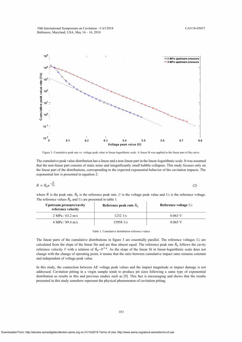
183

Figure 2. An extract of the AE waveform and the envelope function fitted to it.

As observed in figure 2, the envelope follows the waveform, properly addressing the maximum values of each event.If the event contains two distinct peaks, it is assumed that two events are overlapping and both are taken into account.In the area outside the events, the envelope function may create false peaks due to noise and the formulation of thefunction. This effect is negated in the results, as events falling below a certain threshold are considered as either staticnoise or bubble collapses too weak to be erosive.

Results

The peak value distributions for both the 2 MPa and the 4 MPa upstream pressure tests are presented in figure 3. Thedistributions are presented as cumulative so that each rate value represents the rate of voltage peak values larger thanthe corresponding voltage. The bin size for peak counting was 0.02 V. The rate was expressed in [3] and [4] in countsper second per area, with the area being the sensor active area. In this study, the sensor captures all events occurringin the sample, so the active area cannot be properly defined.

Figure 3. Cumulative peak rate vs. voltage peak value in linear-logarithmic scale. A linear fit was applied to the linear part of the curve.

The cumulative peak value distribution has a linear and a non-linear part in the linear-logarithmic scale. It was assumedthat the non-linear part consists of static noise and insignificantly small bubble collapses. This study focuses only onthe linear part of the distributions, corresponding to the expected exponential behavior of the cavitation impacts. Theexponential law is presented in equation 2:

= (2)

where is the peak rate, is the reference peak rate, U is the voltage peak value and U0 is the reference voltage.The reference values and U0 are presented in table 1.

Upstream pressure/cavityreference velocity

Reference peak rate Reference voltage U0

2 MPa / 63.2 m/s 1232 1/s 0.063 V

4 MPa / 89.4 m/s 15958 1/s 0.065 V

Table 1. Cumulative distribution reference values

The linear parts of the cumulative distributions in figure 3 are essentially parallel. The reference voltages U0 arecalculated from the slope of the linear fits and are thus almost equal. The reference peak rate follows the cavityreference velocity V with a relation of ~ . . As the slope of the linear fit in linear-logarithmic scale does notchange with the change of operating point, it means that the ratio between cumulative impact rates remains constantand independent of voltage peak value.

In this study, the connection between AE voltage peak values and the impact magnitude or impact damage is notaddressed. Cavitation pitting in a virgin sample tends to produce pit sizes following a same type of exponentialdistribution as results in this and previous studies such as [9]. This fact is encouraging and shows that the resultspresented in this study somehow represent the physical phenomenon of cavitation pitting.

10th International Symposium on Cavitation - CAV2018

Baltimore, Maryland, USA, May 14 – 16, 2018

CAV18-05037

Downloaded From: http://ebooks.asmedigitalcollection.asme.org on 01/14/2019 Terms of Use: http://www.asme.org/about-asme/terms-of-use

184

Conclusion

A method to monitor and characterize cavitation impacts by acoustic emission was presented. Acoustic emission wasmeasured for two different operating conditions and envelope functions were fitted to the resulting waveforms.Voltage peak values were counted from the fitted envelope functions and cumulative distributions were calculated.Reference peak rates and reference voltages were calculated for both operating points. The reference voltage wasabout the same for both operating points and the reference peak rate had a relation of ~ . .

Using the presented method, the cumulative distributions for acoustic emission voltage peak rate value may becalculated for any operating condition by calculating the reference peak rate Ā and reference voltage U0 and thenapplying the relation between reference peak rates, if the distribution for one point is known. To validate the results,multiple operating points should be tested. With the assumption that the relation holds as stated, the acoustic emissiondistributions can be used in estimating cavitation pitting in the cavitation tunnel. The advantage of the presentedmethod is that it is non-intrusive, as it does not require direct access to the flow. Future studies will address theseissues in more detail. These results show the potential of using acoustic emission in cavitation detection andcharacterization in laboratory testing and eventually in actual hydro machines.

AcknowledgementsThe authors would like to thank Tekes (the Finnish Funding agency for Technology and Innovation), Fortum Powerand Heat Oy, Sandvik Mining and Construction Oy, Valtra Oy and Teollisuuden Voima Oyj for funding the researchand for providing technical support.

References[1] The PREVERO cavitation erosion tunnel. Web page. Available (accessed 13/12/2017): http://www.legi.grenoble-inp.fr/web/spip.php?article1265&lang=fr.[2] Franc, J., Riondet, M., Karimi, A., Chahine, G. (2013). Impact Load Measurements in an Erosive Cavitating Flow. Journal ofFluids Engineering, 133(12).[3] Hujer, J., Carrat, J., Müller, M., Riondet, M. (2015). Impact load measurements with a PVDF pressure sensor in an erosivecavitating flow. Journal of Physics: Conference Series, 656(012051).[4] Franc, J. (2009), Incubation Time and Cavitation Erosion Rate of Work-Hardening Materials. Journal of Fluids Engineering,131(2).[5] Franc, J., Chahine, G., Karimi, A. (2014). Pitting and Incubation period. in: K. Kim, G.L. Chahine, J. Franc, A. Karimi (ed.),10.1007/978-94-017-8539-6. Springer Dordrecht Heidelberg, pp. 37-69.[6] Berchiche, N., Franc, J., Michel, J. (2002). A Cavitation Erosion Model for Ductile Materials. Journal of Fluids Engineering.124(3).[7] Hattori, S., Hirose, T., Sugiyama, K. (2010). Prediction method for cavitation erosion based on measurement of bubble collapseimpact loads. Wear. 269(7-8).[8] Okada, T., Iwai, Y., Hattori, S., Tanimura, N. (1995). Relation between impact load and the damage produced by cavitationbubble collapse. Wear. 184(2).[9] Franc, J., Riondet, M., Karimi, A., Chahine, G. (2012). Material and velocity effects on cavitation erosion pitting. Wear. 274-275.[10] Roy, S.C., Franc, J., Fivel, M. (2015). Cavitation erosion: Using the material as a pressure sensor. Journal of Applied Physics.118(16).[11] Boorsma, A., Fitzsimmons, P. (2009). Quantification of Cavitation Impacts with Acoustic Emissions Techniques. Proceedingsof the 7th International Symposium on Cavitation (CAV).[12] Yongyong, H., Zaiyang, S. (2012). Experimental Research on Cavitation Erosion Detection Based on Acoustic EmissionTechnique. 30th European Conference on Acoustic Emission Testing & 7th International Conference on Acoustic Emission.[13] Schmidt, H., Kirschner, O., Riedelbauch, S., Necker, J., Kopf, E., Rieg, M., Arantes, G., Wessiak, M., Mayrhuber, J. (2014).Influence of the vibro-acoustic sensor position on cavitation detection in a Kaplan turbine. IOP Conference Series: Earth andEnvironmental Science. 22.[14] Schmidt, H., Kirschner, O., Riedelbauch, S. (2014). Cavitation measurements on a pump-turbine model. Journal of Physics:Conference Series. 656(1).[15] van Rijsbergen, M., Foeth, E., Fitzsimmons, P., Boorsma, A. (2012). High-Speed Video Observations and Acoustic-ImpactMeasurements on a NACA 0015 Foil. 8th International Symposium on Cavitation (CAV).[16] Kim, K. Chahine, G., Franc, J., Karimi, A. (2014). Advanced Experimental and Numerical Techniques for Cavitation ErosionPrediction. 1st ed. Springer.

10th International Symposium on Cavitation - CAV2018

Baltimore, Maryland, USA, May 14 – 16, 2018

CAV18-05037

*Corresponding Author, Motohiko Nohmi: nohmi.motohiko@ebara.com

Cavitation CFD Prediction for NACA0015 Hydrofoil Flow Considering Boundary Layer Characteristics

1Motohiko Nohmi*; 1Tomoki Tsuneda; 1Byungjin An; 1Takayuki Suzuki; 2Satoshi Watanabe; 2Shin-ichi Tsuda

1EBARA Corporation, Fujisawa-shi, Kanagawa, Japan; 2Kyushu University, Motooka Nishi-ku, Fukuoka, Japan

Abstract The accuracy of cavitation CFD is not sufficient for the flow around very simple geometries such as single hydrofoil. The lift force and the cavity length are underestimated particularly for the high angle of attack cases. One of the possible reasons of the discrepancy is the singular characteristic of sheet cavitation in the boundary layers that is not taken into account in the recent cavitation models. It was observed that the sheet cavitation is not initiated in the laminar boundary layers. The inception and growth of the sheet cavitation occurs at the reattachment point of the laminar boundary layer separation or at the transition point of the laminar boundary layer to the turbulent boundary layer. These characteristics were reported in many literatures however they are not well modeled for cavitation CFD. In this paper the laminar boundary layer zone is identified for NACA0015 hydrofoil from the high speed video observation. Then, cavitation CFD is carried out by deactivating the cavitation model at the estimated laminar boundary layer zone. This modified cavitation CFD results are discussed and compared to conventional cavitation CFD results and measurement results.

Keywords: cavitation CFD; NACA0015 hydrofoil; boundary layer

Introduction Cavitation CFD prediction functions are built in many commercial codes currently, and are frequently used in the development and design of turbomachinery such as pumps, hydraulic turbines and the ships propellers. On the other hand, whether the analysis accuracy of them is sufficient or not remains a matter of debate. In Japan, the effect of the cavitation coefficient on the lift force of a hydrofoil was analyzed with various kinds of cavitation CFD codes and the prediction performance was evaluated in the “Industry-University Collaborative Research Project on Numerical Predictions of Cavitating Flows in Hydraulic Machinery” conducted in Turbomachinery Society of Japan from 2009 to 2011. As a result, it was found that none of these codes gave sufficient analysis accuracy, and the reliability of cavitation CFD came into question.(1) Responding to this situation, several groups began studies after the project to track down the cause and discuss improvement measures.(2-5) As part of them, this study also conducts an analysis of the NACA0015 hydrofoil that was analyzed in the above project, considering the characteristics of cavitation in a boundary layer that was not considered sufficiently in the existing analysis, and evaluates its effect on analysis accuracy.

Target of the Analysis

The target of the analysis is the flow around the NACA0015 hydrofoil installed in a cavitation tunnel. The result of an experiment conducted in Marine Propeller Cavitation Tunnel at The University of Tokyo is used as the verification data(1). The analytical domain is determined according to this experiment. The shape of the cross section of the measuring part in the tunnel is 600 mm in length and 150 mm in width. The chord length of the NACA0015 hydrofoil is 150 mm and the width 150 mm. In this study the analysis is conducted under the conditions of the inlet flow velocity = 8 m/s (constant) and the angles of attack = 6° and 8°. The analytical domain ranges up to 5C upstream from the center of the chord and down to 5C downstream from it, where C is the length of the chord. For details of other analysis conditions, see the reference (1). The analysis code used in this study is a commercial cord, ANSYS-FLUENT. In a two-dimensional steady analysis, the number of grids is about 90,000, the turbulent model is SST-k-ω model, and the cavitation model is the Zwart-Gerber-Belami model(6).

In this study, the analysis result is arranged using the lift coefficient, Cl, with the cavitation coefficient, σ, and the static pressure coefficient, Cp, defined below:

© 2018 ASME

Downloaded From: http://ebooks.asmedigitalcollection.asme.org on 01/14/2019 Terms of Use: http://www.asme.org/about-asme/terms-of-use

93

PUBLICATIONII

Cavitation E rosion Resistance Assessment and Comparison of ThreeFrancis Turbine Runner Materials

Ylönen, Markku., Saarenrinne, Pentti., Miettinen, Juha., Franc, Jean-Pierre., Fivel,Marc. & Nyyssönen, Tuomo.

Materials Performance and Characterization. 2018, Volume 7, Issue 5, p. 1107-1126.(https://doi.org/10.1520/MPC20180015)

Publication reprinted with kind permission by

ASTM International.

Markku Ylönen,1,2,3,4 Pentti Saarenrinne,2 Juha Miettinen,2 Jean-Pierre Franc,3

Marc Fivel,4 and Tuomo Nyyssönen2

Cavitation Erosion Resistance Assessmentand Comparison of Three Francis TurbineRunner Materials

Reference

Ylönen, M., Saarenrinne, P., Miettinen, J., Franc, J.-P., Fivel, M., and Nyyssönen, T., “Cavitation

Erosion Resistance Assessment and Comparison of Three Francis Turbine Runner Materials,”

Materials Performance and Characterization, Vol. 7, No. 5, 2018, pp. 1107–1126, https://doi.org/

10.1520/MPC20180015. ISSN 2379-1365

ABSTRACT

Cavitation erosion is the most important erosion mechanism in Francis turbine

runner blades. For this reason, knowledge of a material’s ability to resist cavitation is

important in defining how suitable it is for use in a Francis turbine. In this study,

three Francis turbine materials were subjected to cavitation erosion in a high-speed

cavitation tunnel. One of the materials was a low-alloy steel, and the other two

were stainless steels. The cavitation tunnel produced an annular cavitation field on

one face of a cylindrical specimen. The test specimens underwent cavitation

erosion until the erosion had reached a maximum penetration depth of about

0.5 mm. The material surface profiles were measured at regular intervals to

calculate volume and mass loss. These losses were compared to those of several

other materials that had undergone the same tests with the same setup and

operational parameters. The materials were compared according to their steady-

state erosion rates. The steady-state erosion rate represents a material’s ability to

resist cavitation erosion once cavitation damage has already started to develop. The

low-alloy steel eroded four times faster than the two stainless steels. One of the

stainless steels tested here (Stainless steel 1) had the lowest erosion rate, along with

another previously tested stainless steel. The other stainless steel (Stainless steel

2) had a slightly greater erosion rate than the first, falling into the same class as

other lower-grade stainless steels and a nickel aluminum bronze alloy. The results

show that in choosing a turbine blade material, stainless steels outperform

Manuscript received January 30,

2018; accepted for publication

August 8, 2018; published online

October 26, 2018.

1 Université Grenoble Alpes,

1209-1211 Rue de la Piscine,

Saint-Martin-d’Heres, Grenoble

38400, France (Corresponding

author), e-mail: markku.ylonen@

tut.fi, https://orcid.org/0000-

0002-0092-2537

2 Tampere University of

Technology, Korkeakoulunkatu 10,

Tampere 33720, Finland

3 Université Grenoble Alpes, CNRS,

Grenoble INP, LEGI, 1209-1211 Rue

de la Piscine, Grenoble 38400,

France

4 Université Grenoble Alpes, CNRS,

Grenoble INP, SIMAP, 101 Rue de la

Physique, Saint-Martin-d’Heres,

Grenoble 38400, France

Materials Performance and Characterization

Copyright © 2018 by ASTM International, 100 Barr Harbor Drive, PO Box C700, West Conshohocken, PA 19428-2959 1107

doi:10.1520/MPC20180015 / Vol. 7 / No. 5 / 2018 / available online at www.astm.org

nonstainless ones. The choice of which type of stainless steel to use is significant

in turbines with cavitation problems. The eroded surfaces were analyzed with

scanning electron microscopy in order to study the erosion mechanisms, and

these studies showed that most of the damage is probably due to low-cycle fatigue.

Keywords

cavitation, hydro turbine wear, cavitation erosion resistance

Introduction

The use of renewable energy sources, such as wind or solar power, is increasingly common

in electricity production, which means that a large amount of power with modifiable out-

put is required. The current solution is to make more use of hydropower to regulate the

power grid, as this can respond to the rapidly changing demands for power. However,

when the hydropower turbines have to operate outside their optimum operational values,

they experience cavitation and other disturbances. Cavitation erosion is one of the most

significant mechanisms for wear in hydro machines. Therefore, information about the

turbine material’s ability to resist cavitation erosion is vital in avoiding damage or esti-

mating its extent, or both, after it has occurred.

Cavitation occurs in a hydro machine when the local static pressure of a flow falls

below a certain limit, typically close to liquid vapor pressure. At this point, the liquid

evaporates, forming small vapor bubbles that go with the flow. As the static pressure re-

covers, these bubbles collapse violently. Cavitation erosion occurs when a cavitation bub-

ble collapses near a boundary, such as a turbine blade. The presence of the boundary causes

the cavitation bubble to collapse nonsymmetrically, which leads to the formation of a

micro-jet of water that pierces the bubble and a shock wave caused by the collapsing bub-

ble walls [1]. When this micro-jet of water combined with the collapsing bubble ring hits

the boundary, the stress on the material exceeds its yield stress, resulting in microscopic

damage. This microscopic damage accumulates on the material’s surface, eventually lead-

ing to fatigue and rupture on a macroscopic scale.

The main parts of a Francis turbine that suffer from cavitation erosion, along with

their cavitation types, are: (1) the blade suction-side walls, inlet edge cavitation; (2) the

runner blade trailing edges, travelling bubble cavitation; (3) the runner hub walls, inter-

blade cavitating vortices; and (4) the runner blades, leading edge cavitation [2–4]. An ex-

ample of cavitation damage in Francis turbine runner blades, concentrated on the blade’s

trailing edges, is presented in Fig. 1. Cavitation may also occur in the draft tube vortex rope

of a Francis turbine, but there the cavitation bubbles rarely collapse near any boundary

structures.

The development of cavitation erosion in metals has three to four stages: incubation,

acceleration, steady-state, and deceleration [5–9]. In the incubation period, an initially

virgin material surface experiences plastic deformation, but there is negligible overlap

of the cavitation pits. The material’s ability to resist the onset of cavitation erosion is closely

linked to the length of the incubation period. After the incubation period, the material

erosion rate shifts to the acceleration period, when the initial pits start to overlap, and some

of the material starts to rupture, i.e., break away. In the steady-state period, the material loss

through rupture is in a balanced state. As material is removed, new material becomes ex-

posed to cavitation damage. In the deceleration period, if it is reached, the geometry of the

1108 YLÖNEN ET AL. ON TURBINE MATERIAL CAVITATION RESISTANCE

Materials Performance and Characterization

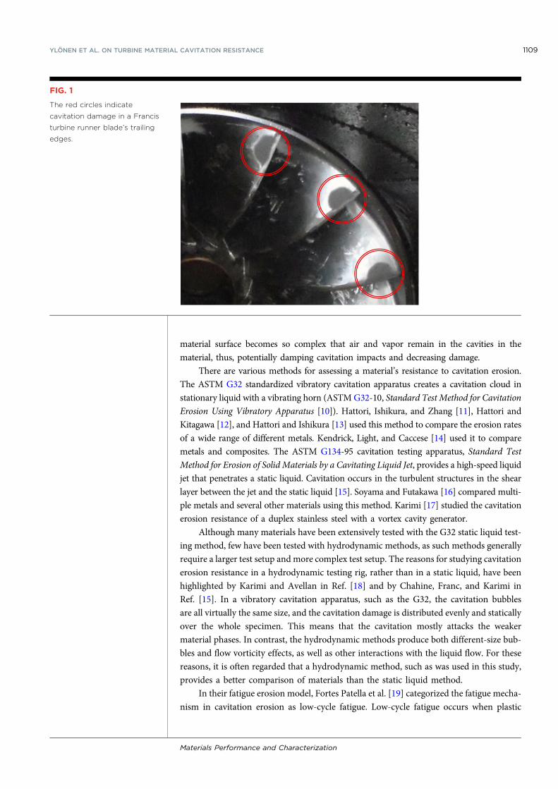
material surface becomes so complex that air and vapor remain in the cavities in the

material, thus, potentially damping cavitation impacts and decreasing damage.

There are various methods for assessing a material’s resistance to cavitation erosion.

The ASTM G32 standardized vibratory cavitation apparatus creates a cavitation cloud in

stationary liquid with a vibrating horn (ASTMG32-10, Standard Test Method for Cavitation

Erosion Using Vibratory Apparatus [10]). Hattori, Ishikura, and Zhang [11], Hattori and

Kitagawa [12], and Hattori and Ishikura [13] used this method to compare the erosion rates

of a wide range of different metals. Kendrick, Light, and Caccese [14] used it to compare

metals and composites. The ASTM G134-95 cavitation testing apparatus, Standard Test

Method for Erosion of Solid Materials by a Cavitating Liquid Jet, provides a high-speed liquid

jet that penetrates a static liquid. Cavitation occurs in the turbulent structures in the shear

layer between the jet and the static liquid [15]. Soyama and Futakawa [16] compared multi-

ple metals and several other materials using this method. Karimi [17] studied the cavitation

erosion resistance of a duplex stainless steel with a vortex cavity generator.

Although many materials have been extensively tested with the G32 static liquid test-

ing method, few have been tested with hydrodynamic methods, as such methods generally

require a larger test setup and more complex test setup. The reasons for studying cavitation

erosion resistance in a hydrodynamic testing rig, rather than in a static liquid, have been

highlighted by Karimi and Avellan in Ref. [18] and by Chahine, Franc, and Karimi in

Ref. [15]. In a vibratory cavitation apparatus, such as the G32, the cavitation bubbles

are all virtually the same size, and the cavitation damage is distributed evenly and statically

over the whole specimen. This means that the cavitation mostly attacks the weaker

material phases. In contrast, the hydrodynamic methods produce both different-size bub-

bles and flow vorticity effects, as well as other interactions with the liquid flow. For these

reasons, it is often regarded that a hydrodynamic method, such as was used in this study,

provides a better comparison of materials than the static liquid method.

In their fatigue erosion model, Fortes Patella et al. [19] categorized the fatigue mecha-

nism in cavitation erosion as low-cycle fatigue. Low-cycle fatigue occurs when plastic

FIG. 1

The red circles indicate

cavitation damage in a Francis

turbine runner blade’s trailing

edges.

YLÖNEN ET AL. ON TURBINE MATERIAL CAVITATION RESISTANCE 1109

Materials Performance and Characterization

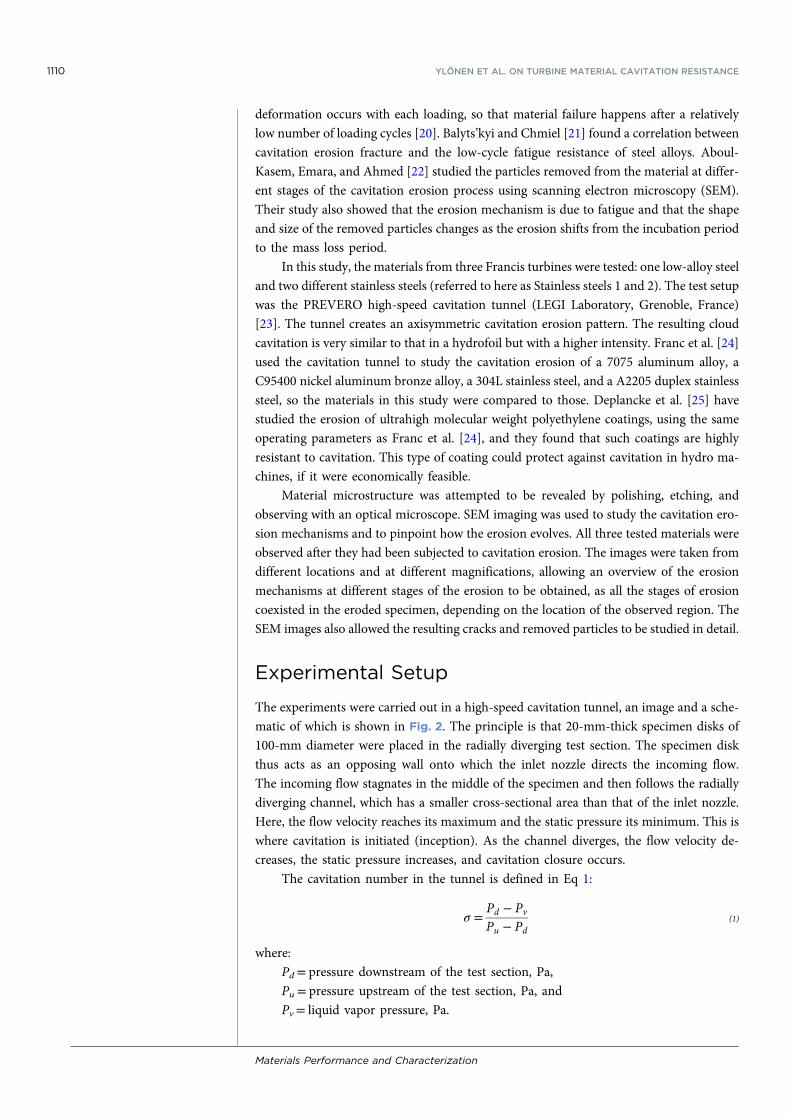
deformation occurs with each loading, so that material failure happens after a relatively

low number of loading cycles [20]. Balyts’kyi and Chmiel [21] found a correlation between

cavitation erosion fracture and the low-cycle fatigue resistance of steel alloys. Aboul-

Kasem, Emara, and Ahmed [22] studied the particles removed from the material at differ-

ent stages of the cavitation erosion process using scanning electron microscopy (SEM).

Their study also showed that the erosion mechanism is due to fatigue and that the shape

and size of the removed particles changes as the erosion shifts from the incubation period

to the mass loss period.

In this study, the materials from three Francis turbines were tested: one low-alloy steel

and two different stainless steels (referred to here as Stainless steels 1 and 2). The test setup

was the PREVERO high-speed cavitation tunnel (LEGI Laboratory, Grenoble, France)

[23]. The tunnel creates an axisymmetric cavitation erosion pattern. The resulting cloud

cavitation is very similar to that in a hydrofoil but with a higher intensity. Franc et al. [24]

used the cavitation tunnel to study the cavitation erosion of a 7075 aluminum alloy, a

C95400 nickel aluminum bronze alloy, a 304L stainless steel, and a A2205 duplex stainless

steel, so the materials in this study were compared to those. Deplancke et al. [25] have

studied the erosion of ultrahigh molecular weight polyethylene coatings, using the same

operating parameters as Franc et al. [24], and they found that such coatings are highly

resistant to cavitation. This type of coating could protect against cavitation in hydro ma-

chines, if it were economically feasible.

Material microstructure was attempted to be revealed by polishing, etching, and

observing with an optical microscope. SEM imaging was used to study the cavitation ero-

sion mechanisms and to pinpoint how the erosion evolves. All three tested materials were

observed after they had been subjected to cavitation erosion. The images were taken from

different locations and at different magnifications, allowing an overview of the erosion

mechanisms at different stages of the erosion to be obtained, as all the stages of erosion

coexisted in the eroded specimen, depending on the location of the observed region. The

SEM images also allowed the resulting cracks and removed particles to be studied in detail.

Experimental Setup

The experiments were carried out in a high-speed cavitation tunnel, an image and a sche-

matic of which is shown in Fig. 2. The principle is that 20-mm-thick specimen disks of

100-mm diameter were placed in the radially diverging test section. The specimen disk

thus acts as an opposing wall onto which the inlet nozzle directs the incoming flow.

The incoming flow stagnates in the middle of the specimen and then follows the radially

diverging channel, which has a smaller cross-sectional area than that of the inlet nozzle.

Here, the flow velocity reaches its maximum and the static pressure its minimum. This is

where cavitation is initiated (inception). As the channel diverges, the flow velocity de-

creases, the static pressure increases, and cavitation closure occurs.

The cavitation number in the tunnel is defined in Eq 1:

σ =Pd − Pv

Pu − Pd

(1)

where:

Pd= pressure downstream of the test section, Pa,

Pu= pressure upstream of the test section, Pa, and

Pv= liquid vapor pressure, Pa.

1110 YLÖNEN ET AL. ON TURBINE MATERIAL CAVITATION RESISTANCE

Materials Performance and Characterization

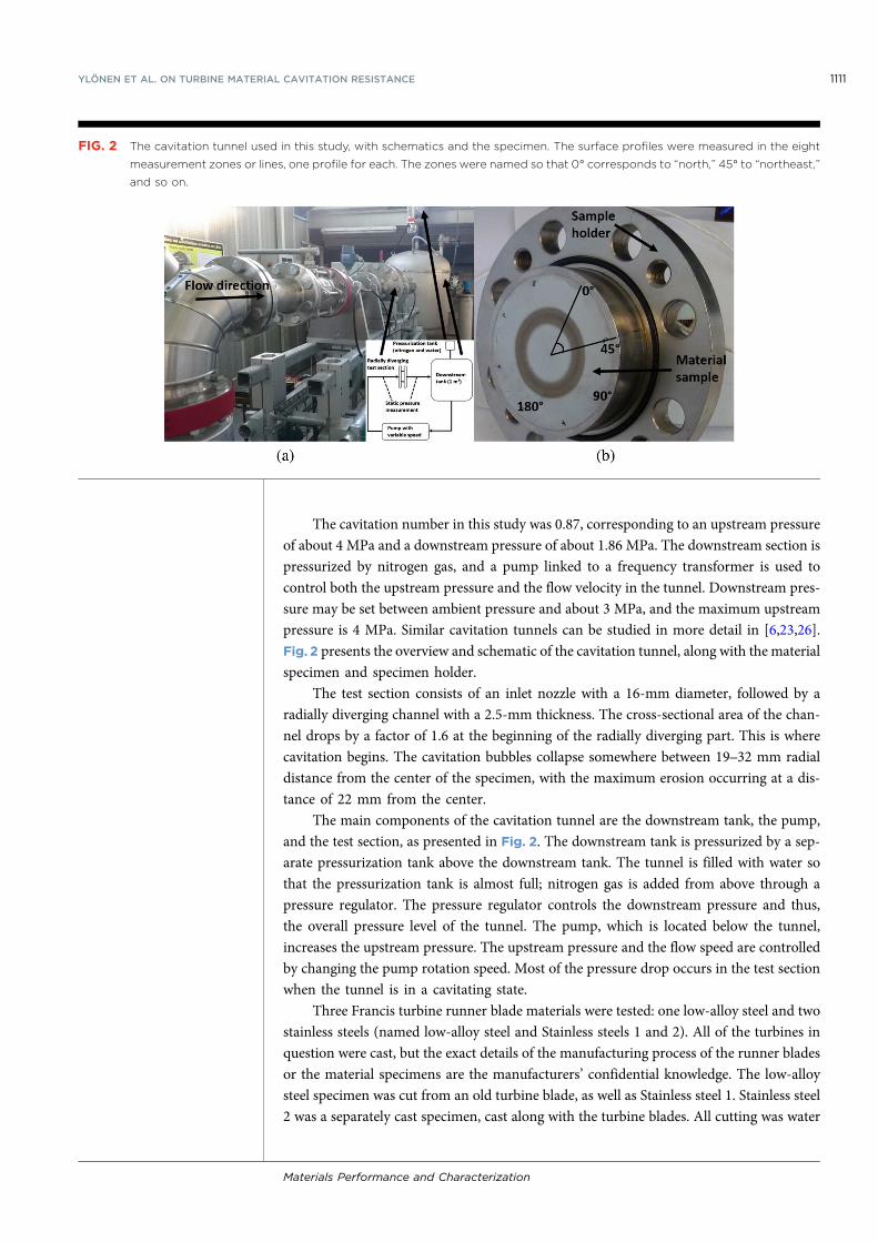
The cavitation number in this study was 0.87, corresponding to an upstream pressure

of about 4 MPa and a downstream pressure of about 1.86 MPa. The downstream section is

pressurized by nitrogen gas, and a pump linked to a frequency transformer is used to

control both the upstream pressure and the flow velocity in the tunnel. Downstream pres-

sure may be set between ambient pressure and about 3 MPa, and the maximum upstream

pressure is 4 MPa. Similar cavitation tunnels can be studied in more detail in [6,23,26].

Fig. 2 presents the overview and schematic of the cavitation tunnel, along with the material

specimen and specimen holder.

The test section consists of an inlet nozzle with a 16-mm diameter, followed by a

radially diverging channel with a 2.5-mm thickness. The cross-sectional area of the chan-

nel drops by a factor of 1.6 at the beginning of the radially diverging part. This is where

cavitation begins. The cavitation bubbles collapse somewhere between 19–32 mm radial

distance from the center of the specimen, with the maximum erosion occurring at a dis-

tance of 22 mm from the center.

The main components of the cavitation tunnel are the downstream tank, the pump,

and the test section, as presented in Fig. 2. The downstream tank is pressurized by a sep-

arate pressurization tank above the downstream tank. The tunnel is filled with water so

that the pressurization tank is almost full; nitrogen gas is added from above through a

pressure regulator. The pressure regulator controls the downstream pressure and thus,

the overall pressure level of the tunnel. The pump, which is located below the tunnel,

increases the upstream pressure. The upstream pressure and the flow speed are controlled

by changing the pump rotation speed. Most of the pressure drop occurs in the test section

when the tunnel is in a cavitating state.

Three Francis turbine runner blade materials were tested: one low-alloy steel and two

stainless steels (named low-alloy steel and Stainless steels 1 and 2). All of the turbines in

question were cast, but the exact details of the manufacturing process of the runner blades

or the material specimens are the manufacturers’ confidential knowledge. The low-alloy

steel specimen was cut from an old turbine blade, as well as Stainless steel 1. Stainless steel

2 was a separately cast specimen, cast along with the turbine blades. All cutting was water

FIG. 2 The cavitation tunnel used in this study, with schematics and the specimen. The surface profiles were measured in the eight

measurement zones or lines, one profile for each. The zones were named so that 0° corresponds to “north,” 45° to “northeast,”

and so on.

YLÖNEN ET AL. ON TURBINE MATERIAL CAVITATION RESISTANCE 1111

Materials Performance and Characterization

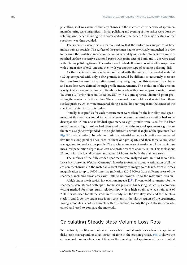
jet cutting, so it was assumed that any changes in the microstructure because of specimen

manufacturing were insignificant. Initial polishing and evening of the surface were done by

rotating sand paper grinding, with water added on the paper. Any major heating of the

specimen was thus avoided.

The specimens were first mirror polished so that the surface was subject to as little

initial strain as possible. The surface of the specimen had to be virtually untouched in order

to measure the cavitation incubation period as accurately as possible. To achieve a mirror-

polished surface, successive diamond pastes with grain sizes of 3 μm and 1 μm were used

with rotating polishing tissues. The surface was finished off using a colloidal silica suspension

with a grain size of 0.03 μm and then with yet another type of rotating polishing disk.

As the specimen mass was large compared with the mass of the eroded material

(1.2 kg compared with only a few grams), it would be difficult to accurately measure

the mass loss because of cavitation erosion by weighing. For this reason, the volume

and mass loss were defined through profile measurements. The evolution of the erosion

was typically measured at four- to five-hour intervals with a contact profilometer (Form

Talysurf 50, Taylor Hobson, Leicester, UK) with a 2-μm spherical diamond point pro-

viding the contact with the surface. The erosion evolution could be calculated from these

surface profiles, which were measured along a radial line running from the center of the

specimen center to its outer edge.

Initially, four profiles for each measurement were taken for the low-alloy steel speci-

men, but this was later found to be inadequate because the erosion evolution had some

discrepancies within one individual specimen, so eight profiles were used for the later

measurements. Eight profiles had been used for the stainless steel specimens right from

the start, as eight corresponded to the eight different azimuthal angles of the specimen (see

Fig. 2 for visualization). In order to minimize potential errors, each profile was measured

five times along parallel lines, each of them one μm apart, and then these values were

averaged out to produce one profile. The specimen underwent erosion until the maximum

measured penetration depth in at least one profile reached about 500 μm. This took about

25 hours for the low-alloy steel and about 65 hours for both the stainless steels.

The surfaces of the fully eroded specimens were analyzed with an SEM (Leo S440,

Leica Microsystems, Wetzlar, Germany). In order to form an accurate estimation of all the

erosion mechanisms in the material, a great variety of images were taken, from 20 times

magnification to up to 5,000 times magnification (20–5,000×) from different areas of the

specimen, including those areas with little to no erosion, up to the maximum erosion.

A high strain rate is typical in cavitation impacts [27]. The material parameters for the

specimens were studied with split Hopkinson pressure bar testing, which is a common

testing method for stress–strain relationships with a high strain rate. A strain rate of

2,000 1/s was used for all the steels in this study, i.e., the low-alloy steel and the Stainless

steels 1 and 2. As the strain rate is not constant in the plastic region of the specimens,

Young’s modulus is not measurable with this method, so only the yield stresses were ob-

tained and used to compare the materials.

Calculating Steady-state Volume Loss Rate

Ten to twenty profiles were obtained for each azimuthal angle for each of the specimen

disks, each corresponding to an instant of time in the erosion process. Fig. 3 shows the

erosion evolution as a function of time for the low-alloy steel specimen with an azimuthal

1112 YLÖNEN ET AL. ON TURBINE MATERIAL CAVITATION RESISTANCE

Materials Performance and Characterization

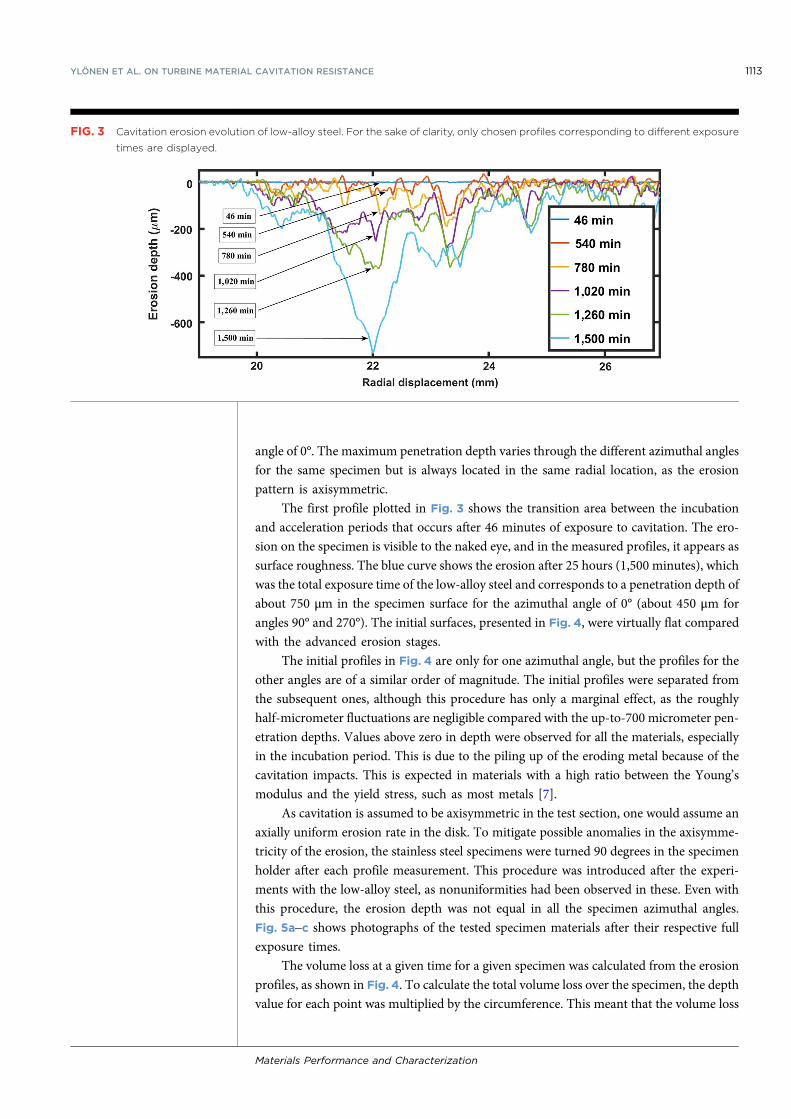
angle of 0°. The maximum penetration depth varies through the different azimuthal angles

for the same specimen but is always located in the same radial location, as the erosion

pattern is axisymmetric.

The first profile plotted in Fig. 3 shows the transition area between the incubation

and acceleration periods that occurs after 46 minutes of exposure to cavitation. The ero-

sion on the specimen is visible to the naked eye, and in the measured profiles, it appears as

surface roughness. The blue curve shows the erosion after 25 hours (1,500 minutes), which

was the total exposure time of the low-alloy steel and corresponds to a penetration depth of

about 750 μm in the specimen surface for the azimuthal angle of 0° (about 450 μm for

angles 90° and 270°). The initial surfaces, presented in Fig. 4, were virtually flat compared

with the advanced erosion stages.

The initial profiles in Fig. 4 are only for one azimuthal angle, but the profiles for the

other angles are of a similar order of magnitude. The initial profiles were separated from

the subsequent ones, although this procedure has only a marginal effect, as the roughly

half-micrometer fluctuations are negligible compared with the up-to-700 micrometer pen-

etration depths. Values above zero in depth were observed for all the materials, especially

in the incubation period. This is due to the piling up of the eroding metal because of the

cavitation impacts. This is expected in materials with a high ratio between the Young’s

modulus and the yield stress, such as most metals [7].

As cavitation is assumed to be axisymmetric in the test section, one would assume an

axially uniform erosion rate in the disk. To mitigate possible anomalies in the axisymme-

tricity of the erosion, the stainless steel specimens were turned 90 degrees in the specimen

holder after each profile measurement. This procedure was introduced after the experi-

ments with the low-alloy steel, as nonuniformities had been observed in these. Even with

this procedure, the erosion depth was not equal in all the specimen azimuthal angles.

Fig. 5a–c shows photographs of the tested specimen materials after their respective full

exposure times.

The volume loss at a given time for a given specimen was calculated from the erosion

profiles, as shown in Fig. 4. To calculate the total volume loss over the specimen, the depth

value for each point was multiplied by the circumference. This meant that the volume loss

FIG. 3 Cavitation erosion evolution of low-alloy steel. For the sake of clarity, only chosen profiles corresponding to different exposure

times are displayed.

YLÖNEN ET AL. ON TURBINE MATERIAL CAVITATION RESISTANCE 1113

Materials Performance and Characterization

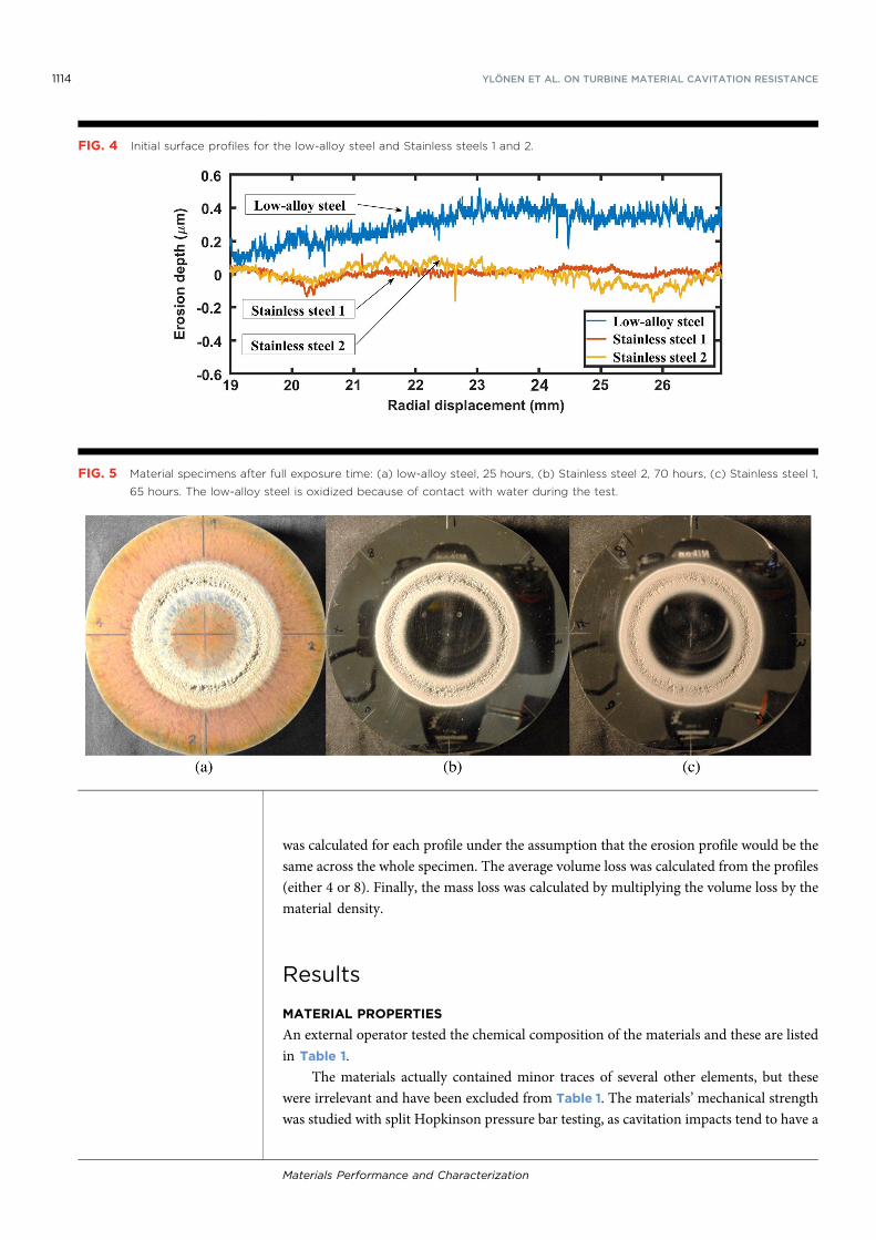
was calculated for each profile under the assumption that the erosion profile would be the

same across the whole specimen. The average volume loss was calculated from the profiles

(either 4 or 8). Finally, the mass loss was calculated by multiplying the volume loss by the

material density.

Results

MATERIAL PROPERTIES

An external operator tested the chemical composition of the materials and these are listed

in Table 1.

The materials actually contained minor traces of several other elements, but these

were irrelevant and have been excluded from Table 1. The materials’ mechanical strength

was studied with split Hopkinson pressure bar testing, as cavitation impacts tend to have a

FIG. 4 Initial surface profiles for the low-alloy steel and Stainless steels 1 and 2.

FIG. 5 Material specimens after full exposure time: (a) low-alloy steel, 25 hours, (b) Stainless steel 2, 70 hours, (c) Stainless steel 1,

65 hours. The low-alloy steel is oxidized because of contact with water during the test.

1114 YLÖNEN ET AL. ON TURBINE MATERIAL CAVITATION RESISTANCE

Materials Performance and Characterization

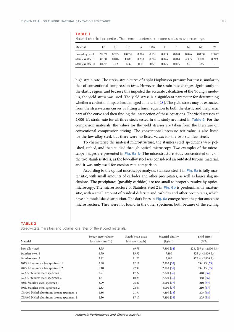
high strain rate. The stress–strain curve of a split Hopkinson pressure bar test is similar to

that of conventional compression tests. However, the strain rate changes significantly in

the elastic region, and because this impeded the accurate calculation of the Young’s modu-

lus, the yield stress was used. The yield stress is a significant parameter for determining

whether a cavitation impact has damaged a material [28]. The yield stress may be extracted

from the stress–strain curves by fitting a linear equation to both the elastic and the plastic

part of the curve and then finding the intersection of these equations. The yield stresses at

2,000 1/s strain rate for all three steels tested in this study are listed in Table 2. For the

comparison materials, the values for the yield stresses are taken from the literature on

conventional compression testing. The conventional pressure test value is also listed

for the low-alloy steel, but there were no listed values for the two stainless steels.

To characterize the material microstructure, the stainless steel specimens were pol-

ished, etched, and then studied through optical microscopy. Two examples of the micro-

scope images are presented in Fig. 6a–b. The microstructure study concentrated only on

the two stainless steels, as the low-alloy steel was considered an outdated turbine material,

and it was only used for erosion rate comparison.

According to the optical microscope analysis, Stainless steel 1 in Fig. 6a is fully mar-

tensitic, with small amounts of carbides and other precipitates, as well as larger slag in-

clusions. The precipitates (possibly carbides) are too small to properly resolve by optical

microscopy. The microstructure of Stainless steel 2 in Fig. 6b is predominantly marten-

sitic, with a small amount of residual δ-ferrite and carbides and other precipitates, which

have a bimodal size distribution. The dark lines in Fig. 6a emerge from the prior austenite

microstructure. They were not found in the other specimen, both because of the etching

TABLE 1

Material chemical properties. The element contents are expressed as mass percentage.

Material Fe C Cr Si Mn P S Ni Mo W

Low-alloy steel 98.69 0.205 0.0051 0.205 0.551 0.033 0.028 0.026 0.0032 0.0077

Stainless steel 1 80.00 0.046 13.80 0.238 0.726 0.026 0.014 4.385 0.201 0.219

Stainless steel 2 81.67 0.02 12.6 0.45 0.58 0.025 0.005 4.2 0.45 –

TABLE 2

Steady-state mass loss and volume loss rates of the studied materials.

Material

Steady-state volume

loss rate (mm3/h)

Steady-state mass

loss rate (mg/h)

Material density

(kg/m3)

Yield stress

(MPa)

Low-alloy steel 8.95 69.79 7,800 [34] 228, 259 at (2,000 1/s)

Stainless steel 1 1.79 13.93 7,800 452 at (2,000 1/s)

Stainless steel 2 2.72 21.23 7,800 477 at (2,000 1/s)

7075 Aluminum alloy specimen 1 7.88 22.12 2,810 [35] 103–145 [35]

7075 Aluminum alloy specimen 2 8.18 22.99 2,810 [35] 103–145 [35]

A2205 Stainless steel specimen 1 2.21 17.27 7,820 [36] 448 [36]

A2205 Stainless steel specimen 2 1.31 10.25 7,820 [36] 448 [36]

304L Stainless steel specimen 1 3.29 26.29 8,000 [37] 210 [37]

304L Stainless steel specimen 2 2.83 22.64 8,000 [37] 210 [37]

C95400 Nickel aluminum bronze specimen 1 2.86 21.34 7,450 [38] 205 [38]

C95400 Nickel aluminum bronze specimen 2 2.30 17.17 7,450 [38] 205 [38]

YLÖNEN ET AL. ON TURBINE MATERIAL CAVITATION RESISTANCE 1115

Materials Performance and Characterization

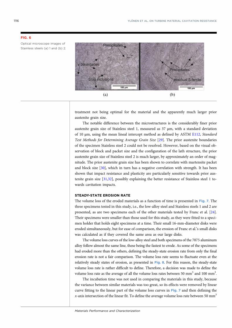
treatment not being optimal for the material and the apparently much larger prior

austenite grain size.

The notable difference between the microstructures is the considerably finer prior

austenite grain size of Stainless steel 1, measured as 37 μm, with a standard deviation

of 10 μm, using the mean lineal intercept method as defined by ASTM E112, Standard

Test Methods for Determining Average Grain Size [29]. The prior austenite boundaries

of the specimen Stainless steel 2 could not be resolved. However, based on the visual ob-

servation of block and packet size and the configuration of the lath structure, the prior

austenite grain size of Stainless steel 2 is much larger, by approximately an order of mag-

nitude. The prior austenite grain size has been shown to correlate with martensite packet

and block size [30], which in turn has a negative correlation with strength. It has been

shown that impact resistance and plasticity are particularly sensitive towards prior aus-

tenite grain size [31,32], possibly explaining the better resistance of Stainless steel 1 to-

wards cavitation impacts.

STEADY-STATE EROSION RATE

The volume loss of the eroded materials as a function of time is presented in Fig. 7. The

three specimens tested in this study, i.e., the low-alloy steel and Stainless steels 1 and 2 are

presented, as are two specimens each of the other materials tested by Franc et al. [24].

Their specimens were smaller than those used for this study, as they were fitted to a speci-

men holder that holds eight specimens at a time. Their small 16-mm-diameter disks were

eroded simultaneously, but for ease of comparison, the erosion of Franc et al.’s small disks

was calculated as if they covered the same area as our large disks.

The volume loss curves of the low-alloy steel and both specimens of the 7075 aluminum

alloy follow almost the same line, these being the fastest to erode. As some of the specimens

had eroded more than the others, defining the steady-state erosion rate from only the final

erosion rate is not a fair comparison. The volume loss rate seems to fluctuate even at the

relatively steady states of erosion, as presented in Fig. 8. For this reason, the steady-state

volume loss rate is rather difficult to define. Therefore, a decision was made to define the

volume loss rate as the average of all the volume loss rates between 50 mm3 and 100 mm3.

The incubation time was not used in comparing the materials in this study, because

the variance between similar materials was too great, so its effects were removed by linear

curve fitting to the linear part of the volume loss curves in Fig. 7 and then defining the

x-axis intersection of the linear fit. To define the average volume loss rate between 50 mm3

FIG. 6

Optical microscope images of

Stainless steels (a) 1 and (b) 2.

1116 YLÖNEN ET AL. ON TURBINE MATERIAL CAVITATION RESISTANCE

Materials Performance and Characterization

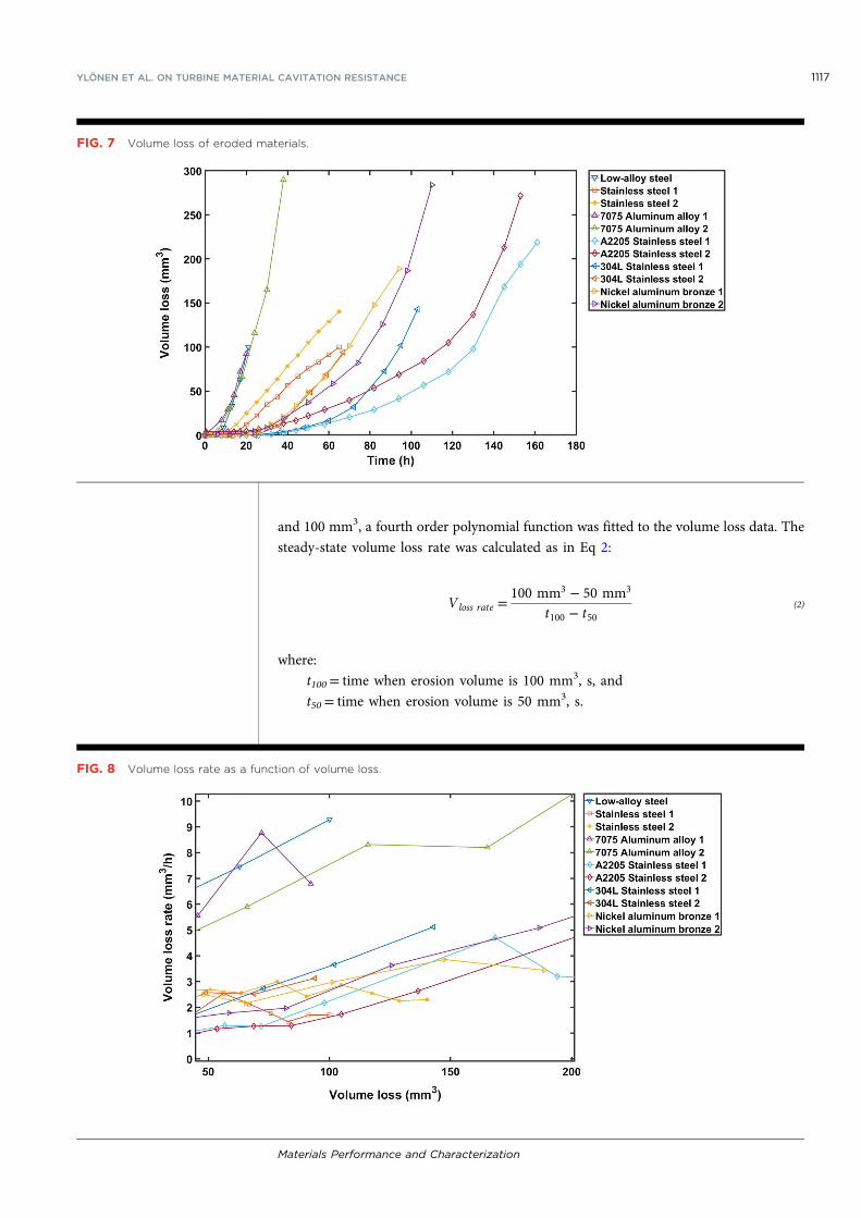
and 100 mm3, a fourth order polynomial function was fitted to the volume loss data. The

steady-state volume loss rate was calculated as in Eq 2:

V loss rate =100 mm3

− 50 mm3

t100 − t50(2)

where:

t100= time when erosion volume is 100 mm3, s, and

t50= time when erosion volume is 50 mm3, s.

FIG. 7 Volume loss of eroded materials.

FIG. 8 Volume loss rate as a function of volume loss.

YLÖNEN ET AL. ON TURBINE MATERIAL CAVITATION RESISTANCE 1117

Materials Performance and Characterization

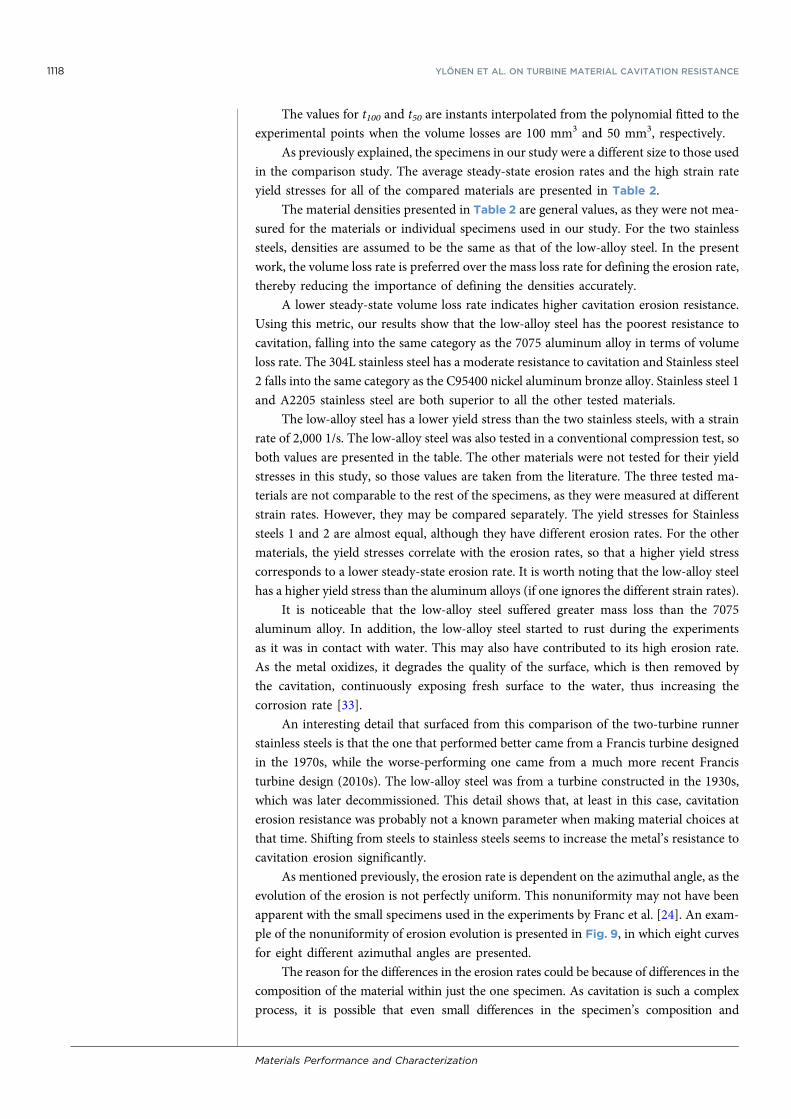
The values for t100 and t50 are instants interpolated from the polynomial fitted to the

experimental points when the volume losses are 100 mm3 and 50 mm3, respectively.

As previously explained, the specimens in our study were a different size to those used

in the comparison study. The average steady-state erosion rates and the high strain rate

yield stresses for all of the compared materials are presented in Table 2.

The material densities presented in Table 2 are general values, as they were not mea-

sured for the materials or individual specimens used in our study. For the two stainless

steels, densities are assumed to be the same as that of the low-alloy steel. In the present

work, the volume loss rate is preferred over the mass loss rate for defining the erosion rate,

thereby reducing the importance of defining the densities accurately.

A lower steady-state volume loss rate indicates higher cavitation erosion resistance.

Using this metric, our results show that the low-alloy steel has the poorest resistance to

cavitation, falling into the same category as the 7075 aluminum alloy in terms of volume

loss rate. The 304L stainless steel has a moderate resistance to cavitation and Stainless steel

2 falls into the same category as the C95400 nickel aluminum bronze alloy. Stainless steel 1

and A2205 stainless steel are both superior to all the other tested materials.

The low-alloy steel has a lower yield stress than the two stainless steels, with a strain

rate of 2,000 1/s. The low-alloy steel was also tested in a conventional compression test, so

both values are presented in the table. The other materials were not tested for their yield

stresses in this study, so those values are taken from the literature. The three tested ma-

terials are not comparable to the rest of the specimens, as they were measured at different

strain rates. However, they may be compared separately. The yield stresses for Stainless

steels 1 and 2 are almost equal, although they have different erosion rates. For the other

materials, the yield stresses correlate with the erosion rates, so that a higher yield stress

corresponds to a lower steady-state erosion rate. It is worth noting that the low-alloy steel

has a higher yield stress than the aluminum alloys (if one ignores the different strain rates).

It is noticeable that the low-alloy steel suffered greater mass loss than the 7075

aluminum alloy. In addition, the low-alloy steel started to rust during the experiments

as it was in contact with water. This may also have contributed to its high erosion rate.

As the metal oxidizes, it degrades the quality of the surface, which is then removed by

the cavitation, continuously exposing fresh surface to the water, thus increasing the

corrosion rate [33].

An interesting detail that surfaced from this comparison of the two-turbine runner

stainless steels is that the one that performed better came from a Francis turbine designed

in the 1970s, while the worse-performing one came from a much more recent Francis

turbine design (2010s). The low-alloy steel was from a turbine constructed in the 1930s,

which was later decommissioned. This detail shows that, at least in this case, cavitation

erosion resistance was probably not a known parameter when making material choices at

that time. Shifting from steels to stainless steels seems to increase the metal’s resistance to

cavitation erosion significantly.

As mentioned previously, the erosion rate is dependent on the azimuthal angle, as the

evolution of the erosion is not perfectly uniform. This nonuniformity may not have been

apparent with the small specimens used in the experiments by Franc et al. [24]. An exam-

ple of the nonuniformity of erosion evolution is presented in Fig. 9, in which eight curves

for eight different azimuthal angles are presented.

The reason for the differences in the erosion rates could be because of differences in the

composition of the material within just the one specimen. As cavitation is such a complex

process, it is possible that even small differences in the specimen’s composition and

1118 YLÖNEN ET AL. ON TURBINE MATERIAL CAVITATION RESISTANCE

Materials Performance and Characterization

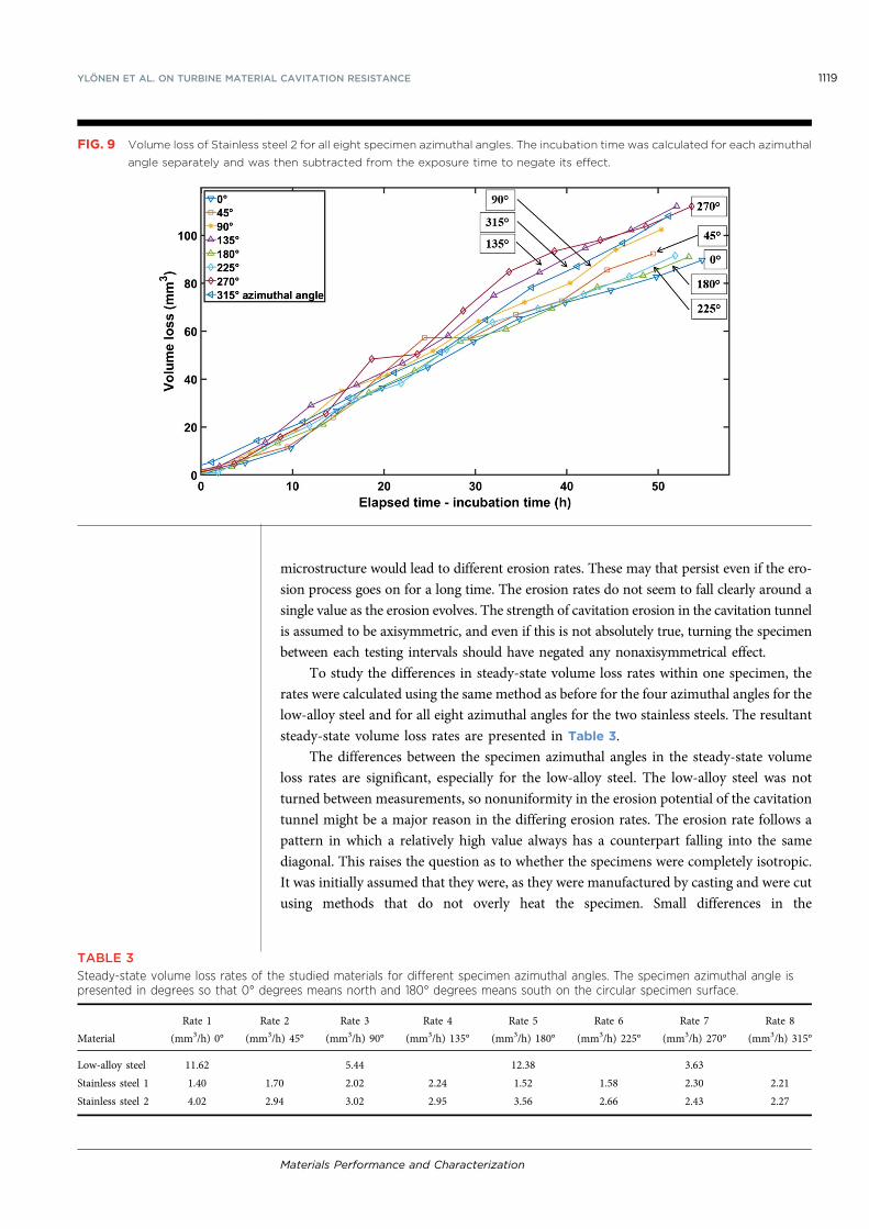
microstructure would lead to different erosion rates. These may that persist even if the ero-

sion process goes on for a long time. The erosion rates do not seem to fall clearly around a

single value as the erosion evolves. The strength of cavitation erosion in the cavitation tunnel

is assumed to be axisymmetric, and even if this is not absolutely true, turning the specimen

between each testing intervals should have negated any nonaxisymmetrical effect.

To study the differences in steady-state volume loss rates within one specimen, the

rates were calculated using the same method as before for the four azimuthal angles for the

low-alloy steel and for all eight azimuthal angles for the two stainless steels. The resultant

steady-state volume loss rates are presented in Table 3.

The differences between the specimen azimuthal angles in the steady-state volume

loss rates are significant, especially for the low-alloy steel. The low-alloy steel was not

turned between measurements, so nonuniformity in the erosion potential of the cavitation

tunnel might be a major reason in the differing erosion rates. The erosion rate follows a

pattern in which a relatively high value always has a counterpart falling into the same

diagonal. This raises the question as to whether the specimens were completely isotropic.

It was initially assumed that they were, as they were manufactured by casting and were cut

using methods that do not overly heat the specimen. Small differences in the

FIG. 9 Volume loss of Stainless steel 2 for all eight specimen azimuthal angles. The incubation time was calculated for each azimuthal

angle separately and was then subtracted from the exposure time to negate its effect.

TABLE 3

Steady-state volume loss rates of the studied materials for different specimen azimuthal angles. The specimen azimuthal angle is

presented in degrees so that 0° degrees means north and 180° degrees means south on the circular specimen surface.

Material

Rate 1

(mm3/h) 0°

Rate 2

(mm3/h) 45°

Rate 3

(mm3/h) 90°

Rate 4

(mm3/h) 135°

Rate 5

(mm3/h) 180°

Rate 6

(mm3/h) 225°

Rate 7

(mm3/h) 270°

Rate 8

(mm3/h) 315°

Low-alloy steel 11.62 5.44 12.38 3.63

Stainless steel 1 1.40 1.70 2.02 2.24 1.52 1.58 2.30 2.21

Stainless steel 2 4.02 2.94 3.02 2.95 3.56 2.66 2.43 2.27

YLÖNEN ET AL. ON TURBINE MATERIAL CAVITATION RESISTANCE 1119

Materials Performance and Characterization

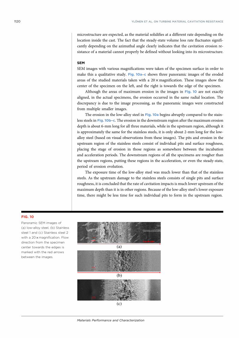
microstructure are expected, as the material solidifies at a different rate depending on the

location inside the cast. The fact that the steady-state volume loss rate fluctuates signifi-

cantly depending on the azimuthal angle clearly indicates that the cavitation erosion re-

sistance of a material cannot properly be defined without looking into its microstructure.

SEM

SEM images with various magnifications were taken of the specimen surface in order to

make this a qualitative study. Fig. 10a–c shows three panoramic images of the eroded

areas of the studied materials taken with a 20 ×magnification. These images show the

center of the specimen on the left, and the right is towards the edge of the specimen.

Although the areas of maximum erosion in the images in Fig. 10 are not exactly

aligned, in the actual specimens, the erosion occurred in the same radial location. The

discrepancy is due to the image processing, as the panoramic images were constructed

from multiple smaller images.

The erosion in the low-alloy steel in Fig. 10a begins abruptly compared to the stain-

less steels in Fig. 10b–c. The erosion in the downstream region after the maximum erosion

depth is about 6-mm long for all three materials, while in the upstream region, although it

is approximately the same for the stainless steels, it is only about 2-mm long for the low-

alloy steel (based on visual observations from these images). The pits and erosion in the

upstream region of the stainless steels consist of individual pits and surface roughness,

placing the stage of erosion in those regions as somewhere between the incubation

and acceleration periods. The downstream regions of all the specimens are rougher than

the upstream regions, putting these regions in the acceleration, or even the steady-state,

period of erosion evolution.

The exposure time of the low-alloy steel was much lower than that of the stainless

steels. As the upstream damage to the stainless steels consists of single pits and surface

roughness, it is concluded that the rate of cavitation impacts is much lower upstream of the

maximum depth than it is in other regions. Because of the low-alloy steel’s lower exposure

time, there might be less time for such individual pits to form in the upstream region.

FIG. 10

Panoramic SEM images of

(a) low-alloy steel, (b) Stainless

steel 1 and (c) Stainless steel 2

with a 20 ×magnification. Flow

direction from the specimen

center towards the edges is

marked with the red arrows

between the images.

1120 YLÖNEN ET AL. ON TURBINE MATERIAL CAVITATION RESISTANCE

Materials Performance and Characterization

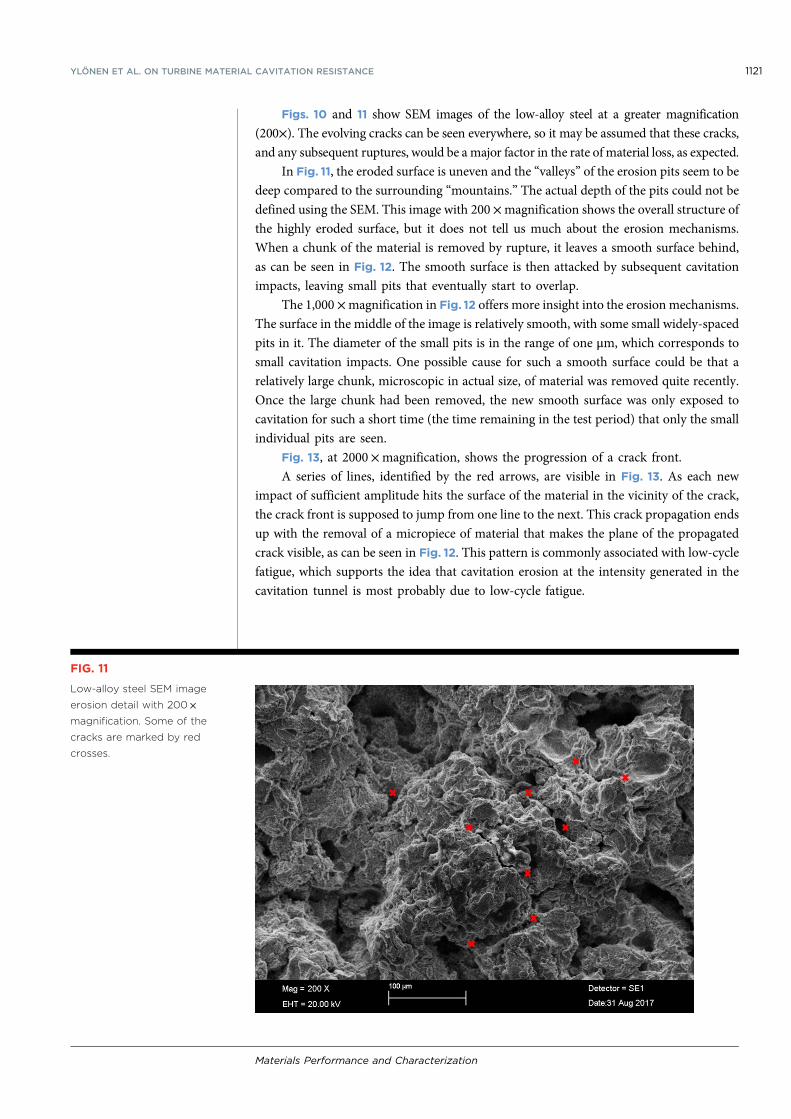
Figs. 10 and 11 show SEM images of the low-alloy steel at a greater magnification

(200×). The evolving cracks can be seen everywhere, so it may be assumed that these cracks,

and any subsequent ruptures, would be a major factor in the rate of material loss, as expected.

In Fig. 11, the eroded surface is uneven and the “valleys” of the erosion pits seem to be

deep compared to the surrounding “mountains.” The actual depth of the pits could not be

defined using the SEM. This image with 200 ×magnification shows the overall structure of

the highly eroded surface, but it does not tell us much about the erosion mechanisms.

When a chunk of the material is removed by rupture, it leaves a smooth surface behind,

as can be seen in Fig. 12. The smooth surface is then attacked by subsequent cavitation

impacts, leaving small pits that eventually start to overlap.

The 1,000 ×magnification in Fig. 12 offers more insight into the erosion mechanisms.

The surface in the middle of the image is relatively smooth, with some small widely-spaced

pits in it. The diameter of the small pits is in the range of one μm, which corresponds to

small cavitation impacts. One possible cause for such a smooth surface could be that a

relatively large chunk, microscopic in actual size, of material was removed quite recently.

Once the large chunk had been removed, the new smooth surface was only exposed to

cavitation for such a short time (the time remaining in the test period) that only the small

individual pits are seen.

Fig. 13, at 2000 ×magnification, shows the progression of a crack front.

A series of lines, identified by the red arrows, are visible in Fig. 13. As each new

impact of sufficient amplitude hits the surface of the material in the vicinity of the crack,

the crack front is supposed to jump from one line to the next. This crack propagation ends

up with the removal of a micropiece of material that makes the plane of the propagated

crack visible, as can be seen in Fig. 12. This pattern is commonly associated with low-cycle

fatigue, which supports the idea that cavitation erosion at the intensity generated in the

cavitation tunnel is most probably due to low-cycle fatigue.

FIG. 11

Low-alloy steel SEM image

erosion detail with 200 ×

magnification. Some of the

cracks are marked by red

crosses.

YLÖNEN ET AL. ON TURBINE MATERIAL CAVITATION RESISTANCE 1121

Materials Performance and Characterization

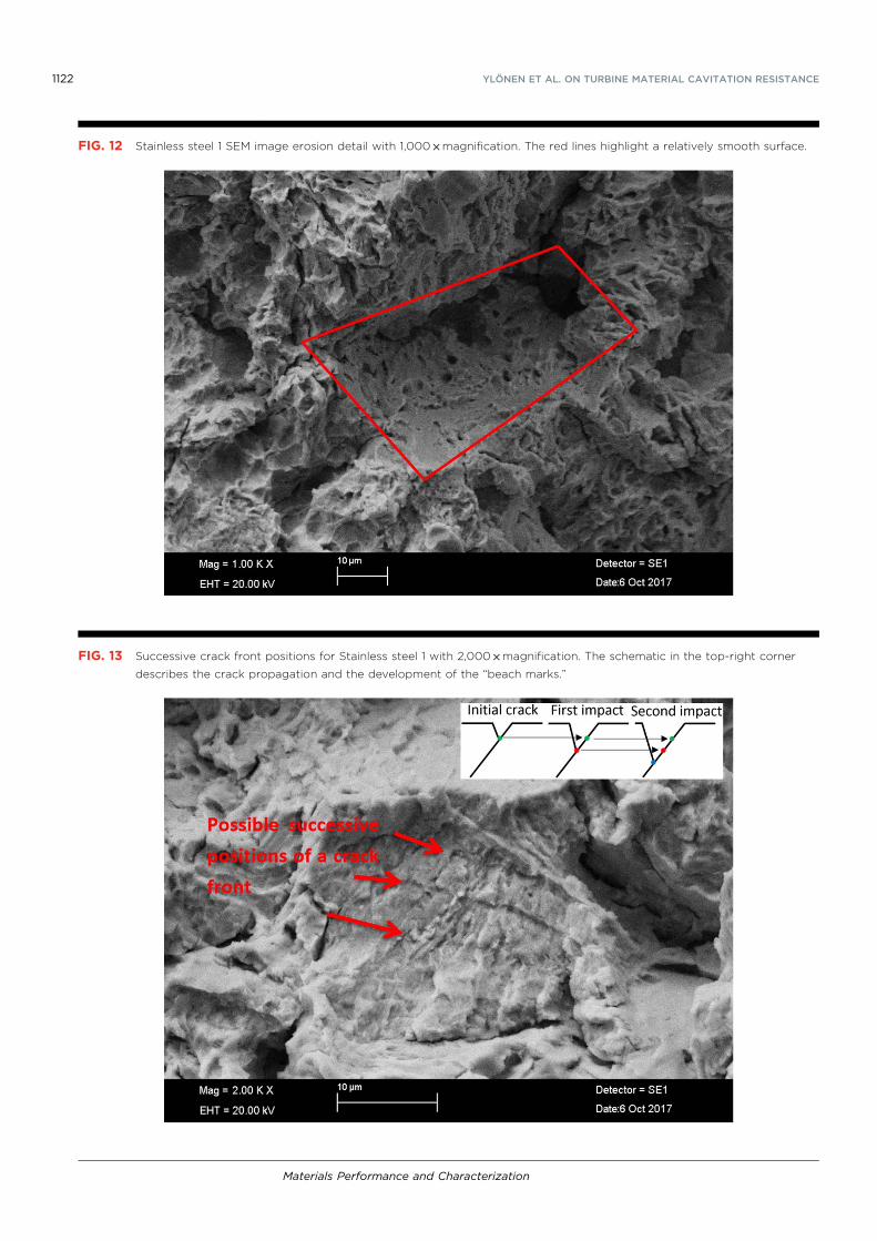
FIG. 12 Stainless steel 1 SEM image erosion detail with 1,000 ×magnification. The red lines highlight a relatively smooth surface.

FIG. 13 Successive crack front positions for Stainless steel 1 with 2,000 ×magnification. The schematic in the top-right corner

describes the crack propagation and the development of the “beach marks.”

1122 YLÖNEN ET AL. ON TURBINE MATERIAL CAVITATION RESISTANCE

Materials Performance and Characterization

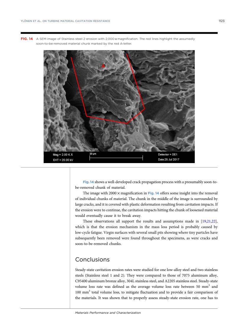
Fig. 14 shows a well-developed crack propagation process with a presumably soon-to-

be-removed chunk of material.

The image with 2000 ×magnification in Fig. 14 offers some insight into the removal

of individual chunks of material. The chunk in the middle of the image is surrounded by

large cracks, and it is covered with plastic deformation resulting from cavitation impacts. If

the erosion were to continue, the cavitation impacts hitting the chunk of loosened material

would eventually cause it to break away.

These observations all support the results and assumptions made in [19,21,22],

which is that the erosion mechanism in the mass loss period is probably caused by

low-cycle fatigue. Virgin surfaces with several small pits showing where tiny particles have

subsequently been removed were found throughout the specimens, as were cracks and

soon-to-be-removed chunks.

Conclusions

Steady-state cavitation erosion rates were studied for one low-alloy steel and two stainless

steels (Stainless steel 1 and 2). They were compared to those of 7075 aluminum alloy,

C95400 aluminum bronze alloy, 304L stainless steel, and A2205 stainless steel. Steady-state

volume loss rate was defined as the average volume loss rate between 50 mm3 and

100 mm3 total volume loss, to mitigate fluctuation and to provide a fair comparison of

the materials. It was shown that to properly assess steady-state erosion rate, one has to

FIG. 14 A SEM image of Stainless steel 2 erosion with 2,000 ×magnification. The red lines highlight the assumedly

soon-to-be-removed material chunk marked by the red A-letter.

YLÖNEN ET AL. ON TURBINE MATERIAL CAVITATION RESISTANCE 1123

Materials Performance and Characterization

average several erosion processes through the specimen. The stainless steels were speci-

mens from turbines that are of a type that is still in use, so they are relevant in the field of

turbine design.

The low-alloy steel had the poorest cavitation erosion resistance, along with the 7075

aluminum alloy. In this study, 304L stainless steel, C95400 aluminum bronze alloy, and

Stainless steel 2 had a better resistance than the other materials, while A2205 stainless steel

and Stainless steel 1 had the highest cavitation erosion resistance. It was found that the

erosion rates differ significantly even within one specimen. This means that assessing a

single value for cavitation erosion resistance is problematic, because factors, such as small

differences in the local material composition or microstructure, might change the erosion

rates significantly. Even minor anisotropies in the specimen material might be the cause of

significantly differing erosion rates, as it was observed that the erosion rates are either high

or low along the same diagonal in a circular specimen. This means that in hydro machines,

cavitation erosion rates may also differ greatly, depending on how, for example, the casting

process leads to different grain sizes in the machine.

Materials with low steady-state erosion rates and therefore, high cavitation erosion

resistances, generally had a higher yield stress. The yield stress, however, cannot be used

alone to estimate the erosion rate, as Stainless steel 2 had a slightly higher yield stress than

Stainless steel 1, for example, but it also had a higher erosion rate. Furthermore, the low-

alloy steel had a higher yield stress than the 7075 aluminum alloy, but both materials

eroded at the same rate. This was probably due to the combined effect of corrosion

and cavitation erosion.

The material microstructure analysis showed that Stainless steels 1 and 2 consist of

almost 100 % martensite and that the first one has a significantly smaller prior austenite

grain size. The prior austenite grain size is related to the impact strength and plasticity, so

this could explain the difference in erosion rate between these two martensitic steels.

SEM images were taken from three eroded specimens, and they were analyzed to

observe the erosion mechanisms. The images showed the dominating erosion mechanism

to be, most probably, low-cycle fatigue. Virgin areas were found, with recently removed

material and pits resulting from plastic deformations. Cracks and presumably soon-to-be-

removed chunks of material were observed throughout the specimens. So-called “beach

marks” were also found, indicating towards low-cycle fatigue.

ACKNOWLEDGMENTS

The authors would like to thank Business Finland, Fortum Power and Heat Oy, Sandvik

Mining and Construction Oy, Valtra Oy, and Teollisuuden Voima Oyj for funding the

research and for providing technical support.

References

[1] Brennen, C. E., “Cavitation Bubble Collapse,” Cavitation and Bubble Dynamics,Oxford University Press, Oxford, UK, 1995, pp. 80–108.

[2] Avellan, F., “Introduction to Cavitation in Hydraulic Machinery,” presented at theSixth International Conference on Hydraulic Machinery and Hydrodynamics,Timisoara, Romania, Oct. 21–22, 2004, Politehnica University of Timişoara,Timisoara, Romania.

[3] Kumar, P. and Saini, R. P., “Study of Cavitation in Hydro Turbines—A Review,”Renew. Sustainable Energy Rev., Vol. 14, No. 1, 2010, pp. 374–383, https://doi.org/10.1016/j.rser.2009.07.024

1124 YLÖNEN ET AL. ON TURBINE MATERIAL CAVITATION RESISTANCE

Materials Performance and Characterization

[4] Escaler, X., Egusquiza, E., Farhat, M., Avellan, F., and Coussirat, M., “Detection ofCavitation in Hydraulic Turbines,” Mech. Syst. Sig. Process., Vol. 20, No. 4, 2006,pp. 983–1007, https://doi.org/10.1016/j.ymssp.2004.08.006

[5] Berchiche, N., Franc, J. P., and Michel, J. M., “A Cavitation Erosion Model for DuctileMaterials,” J. Fluids Eng., Vol. 124, No. 3, 2002, pp. 601–606, https://doi.org/10.1115/1.1486474

[6] Franc, J. P., “Incubation Time and Cavitation Erosion Rate of Work-HardeningMaterials,” J. Fluids Eng., Vol. 131, No. 2, 2009, p. 021303, https://doi.org/10.1115/1.3063646

[7] Franc, J. P., Chahine, G. L., and Karimi, A., “Pitting and Incubation Period,”Advanced Experimental and Numerical Techniques for Cavitation ErosionPrediction, Springer Dordrecht Heidelberg, Heidelberg, Germany, 2014, pp. 37–69.

[8] Zhou, Y. K. and Hammitt, F. G., “Cavitation Erosion Incubation Period,” Wear,Vol. 86, No. 2, 1983, pp. 299–313, https://doi.org/10.1016/0043-1648(83)90168-0

[9] Chahine, G. L., Franc, J. P., and Karimi, A., “Mass Loss and Advanced Periods ofErosion,” Advanced Experimental and Numerical Techniques for CavitationErosion Prediction, Springer Dordrecht Heidelberg, Heidelberg, Germany, 2014,pp. 97–121.

[10] ASTM G32-10, Standard Test Method for Cavitation Erosion Using VibratoryApparatus, ASTM International, West Conshohocken, PA, 2010, www.astm.org

[11] Hattori, S., Ishikura, R., and Zhang, Q., “Construction of Database on CavitationErosion and Analyses of Carbon Steel Data,” Wear, Vol. 257, Nos. 9–10, 2004,pp. 1022–1029, https://doi.org/10.1016/j.wear.2004.07.002

[12] Hattori, S. and Kitagawa, T., “Analysis of Cavitation Erosion Resistance of CastIron and Nonferrous Metals Based on Database and Comparison with CarbonSteel Data,” Wear, Vol. 269, Nos. 5–6, 2010, pp. 443–448, https://doi.org/10.1016/j.wear.2010.04.031

[13] Hattori, S. and Ishikura, R., “Revision of Cavitation Erosion Database and Analysis ofStainless Steel Data,”Wear, Vol. 268, Nos. 1–2, 2010, pp. 109–116, https://doi.org/10.1016/j.wear.2009.07.005

[14] Kendrick, H., Light, M. S., and Caccese, V., Development of a Cavitation ErosionResistant Advanced Material System, Report No. UM-MACH-RPT-01-05, Office ofNaval Research, Arlington, VA, 2005, 67p.

[15] Chahine, G. L., Franc, J. P., and Karimi, A., “Laboratory Testing Methods ofCavitation Erosion,” Advanced Experimental and Numerical Techniques forCavitation Erosion Prediction, Springer Dordrecht Heidelberg, Heidelberg, Germany,2014, pp. 21–35.

[16] Soyama, H. and Futakawa, M., “Estimation of Incubation Time of Cavitation Erosionfor Various Cavitating Conditions,” Tribol. Lett., Vol. 17, No. 1, 2004, pp. 27–30,https://doi.org/10.1023/B:TRIL.0000017415.79517.8c

[17] Karimi, A., “Cavitation Erosion of a Duplex Stainless Steel,”Mater. Sci. Eng., Vol. 86,1987, pp. 191–203, https://doi.org/10.1016/0025-5416(87)90452-6

[18] Karimi, A. and Avellan, F., “Comparison of Erosion Mechanisms in Different Typesof Cavitation,” Wear, Vol. 113, No. 3, 1986, pp. 305–322, https://doi.org/10.1016/0043-1648(86)90031-1

[19] Fortes Patella, R., Choffat, T., Reboud, J., and Archer, A., “Mass Loss Simulation inCavitation Erosion: Fatigue Criterion Approach,” Wear, Vol. 300, No. 1, 2013,pp. 205–215, https://doi.org/10.1016/j.wear.2013.01.118

[20] Bathias, C. and Pineau, A., “Low-Cycle Fatigue,” Fatigue of Materials and Structures:Fundamentals, John Wiley & Sons, New York, NY, 2010, pp. 113–116, https://doi.org/10.1002/9781118623435

[21] Balyts’kyi, O. I. and Chmiel, J., “Resistance of Plate Shipbuilding Steels to Cavitation-Erosion and Fatigue Fracture,”Mater. Sci., Vol. 50, No. 5, 2015, pp. 736–739, https://doi.org/10.1007/s11003-015-9779-y

YLÖNEN ET AL. ON TURBINE MATERIAL CAVITATION RESISTANCE 1125

Materials Performance and Characterization

[22] Abouel-Kasem, A., Emara, K. M., and Ahmed, S. M., “Characterizing CavitationErosion Particles by Analysis of SEM Images,” Tribol. Int., Vol. 42, No. 1, 2009,pp. 130–136, https://doi.org/10.1016/j.triboint.2008.05.008

[23] Laboratoire LEGI, “The PREVERO Cavitation Erosion Tunnel,” Laboratoire LEGI,2018, https://web.archive.org/web/20180327065723/https://www.legi.grenoble-inp.fr/web/spip.php?article1265&lang=fr (accessed 27 March 2018).

[24] Franc, J. P., Riondet, M., Karimi, A., and Chahine, G. L., “Material and VelocityEffects on Cavitation Erosion Pitting,” Wear, Vols. 274–275, 2012, pp. 248–259,https://doi.org/10.1016/j.wear.2011.09.006

[25] Deplancke, T., Lame, O., Cavaille, J., Fivel, M., Riondet, M., and Franc, J. P.,“Outstanding Cavitation Erosion Resistance of Ultra High Molecular WeightPolyethylene (UHMWPE) Coatings,” Wear, Vols. 328–329, 2015, pp. 301–308,https://doi.org/10.1016/j.wear.2015.01.077

[26] Ylönen, M., Saarenrinne, P., Miettinen, J., Franc, J. P., and Fivel, M., “CavitationBubble Collapse Monitoring by Acoustic Emission in Laboratory Testing,” presentedat the Tenth International Symposium on Cavitation (CAV2018), Baltimore, MD,May 14–16, 2018, Johns Hopkins University, Baltimore, MD—unpublished.

[27] Chahine, G. L., Franc, J. P., and Karimi, A., “Cavitation and Cavitation Erosion,”Advanced Experimental and Numerical Techniques for Cavitation ErosionPrediction, Springer Dordrecht Heidelberg, Heidelberg, Germany, 2014, pp. 3–20,https://doi.org/10.1007/978-94-017-8539-6

[28] ASTM E112-13, Standard Test Methods for Determining Average Grain Size, ASTMInternational, West Conshohocken, PA, 2013, www.astm.org

[29] Morito, S., Yoshida, H., Maki, T., and Huang, X., “Effect of Block Size on the Strengthof Lath Martensite in Low Carbon Steels,” Mater. Sci. Eng. A, Vols. 438–440, 2006,pp. 237–240, https://doi.org/10.1016/j.msea.2005.12.048

[30] Roy, S. C., 2015, “Modeling and Analysis of Material Behavior during CavitationErosion,” Ph.D. dissertation, Université Grenoble Alpes, Grenoble, France.

[31] Zavaleta Gutiérrez, N., Luppo, M. I., Danon, C. A., Toda-Caraballo, I., Capdevila, C., andGarcía, D. A., “Heterogeneous Austenite Grain Growth inMartensitic 9Cr Steel: CoupledInfluence of Initial Metallurgical State and Heating Rate,” Mater. Sci. Technol., Vol. 29,No. 10, 2013, pp. 1254–1266, https://doi.org/10.1179/1743284713Y.0000000271

[32] Kim, H. J., Kim, Y. H., and Morris, Jr., J. W., “Thermal Mechanisms of Grain andPacket Refinement in a Lath Martensitic Steel,” ISIJ Int., Vol. 38, No. 11, 1998,pp. 1277–1285, https://doi.org/10.2355/isijinternational.38.1277

[33] Ryl, J., Darowicki, K., and Slepski, P., “Evaluation of Cavitation Erosion-CorrosionDegradation of Mild Steel by Means of Dynamic Impedance Spectroscopy inGalvanostatic Mode,” Corros. Sci., Vol. 53, No. 5, 2011, pp. 1873–1879, https://doi.org/10.1016/j.corsci.2011.02.004

[34] MatWeb, “Overview of Materials for Low Alloy Steel,” 2018, MatWeb MaterialProperty Data, http://web.archive.org/web/20180921140451/http://www.matweb.com/search/datasheettext.aspx?matguid=d1bdbccde4da4da4a9dbb8918d783b29(accessed 27 March 2018).

[35] MatWeb, “Aluminum 7075-O,” 2018, Matweb Material Property Data, http://www.matweb.com/search/DataSheet.aspx?MatGUID=da98aea5e9de44138a7d28782f60a836&ckck=1 (accessed 27 March 2018).

[36] MatWeb, “Carlson 2205 (UNS S32205) Duplex Stainless Steel,” 2018, MatWeb MaterialProperty Data, http://web.archive.org/web/20180921140647/http://www.matweb.com/search/datasheettext.aspx?matguid=086d8b05d09c4963b95253bd278dc4f4 (accessed 27March 2018).

[37] MatWeb, “AISI Type 304L Stainless Steel,” 2018, MatWebMaterial Property Data, http://web.archive.org/web/20180921140725/http://www.matweb.com/search/datasheet_print.aspx?matguid=e2147b8f727343b0b0d51efe02a6127e (accessed 27 March 2018).

[38] MatWeb, “Aluminum Bronze, UNS C95400, Copper Casting Alloy, As Cast,” 2018,MatWeb Material Property Data, http://web.archive.org/web/20180921140819/http://www.matweb.com/search/datasheettext.aspx?matid=11963 (accessed 27 March 2018).

1126 YLÖNEN ET AL. ON TURBINE MATERIAL CAVITATION RESISTANCE

Copyright by ASTM International (all rights reserved), pursuant to License Agreement. No further reproduction authorized.

94

PUBLICATIONIII

E stimation of Cavitation Pit Distributions by Acoustic E mission

Ylönen, Markku., Saarenrinne, Pentti., Miettinen, Juha., Franc, Jean-Pierre., Fivel,Marc. & Laakso, Jarmo.

Journal of Hydraulic Engineering. 2019, Volume 146, Issue 2, p. 1-11.(https://doi.org/10.1061/(ASCE)HY.1943-7900.0001686)

Publication reprinted with kind permission by

The American Society of Civil E ngineers.

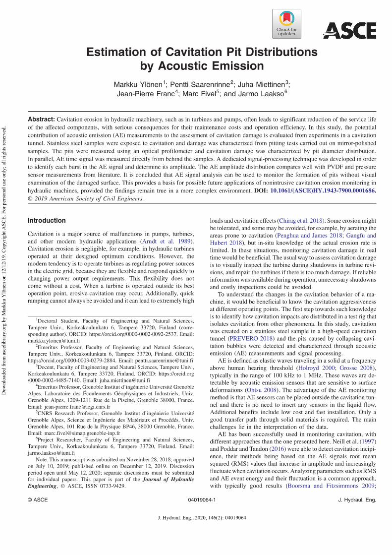
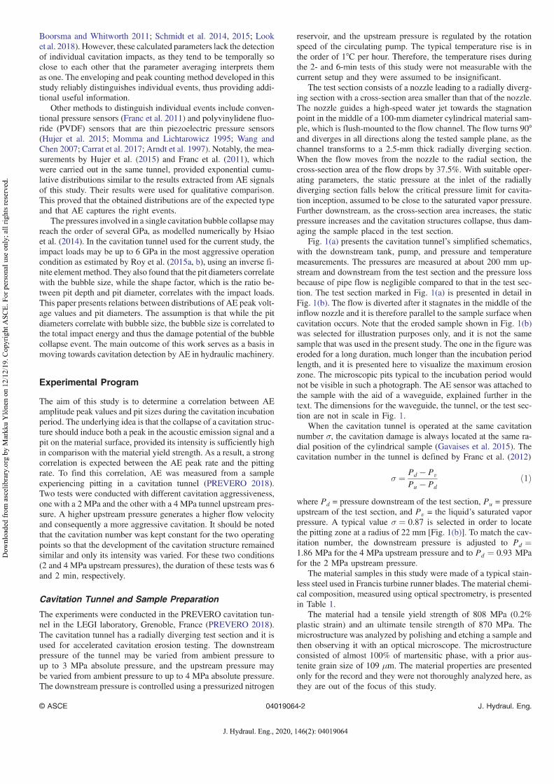
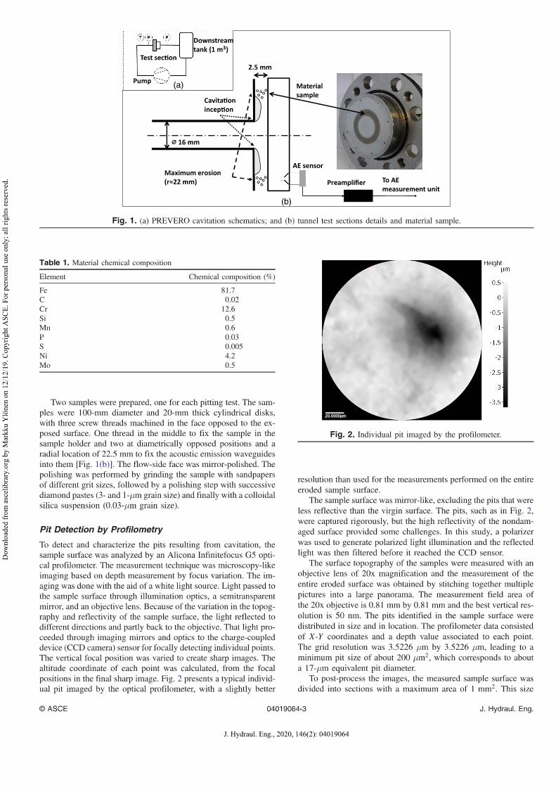
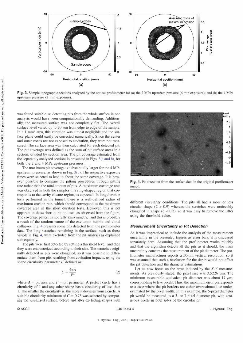
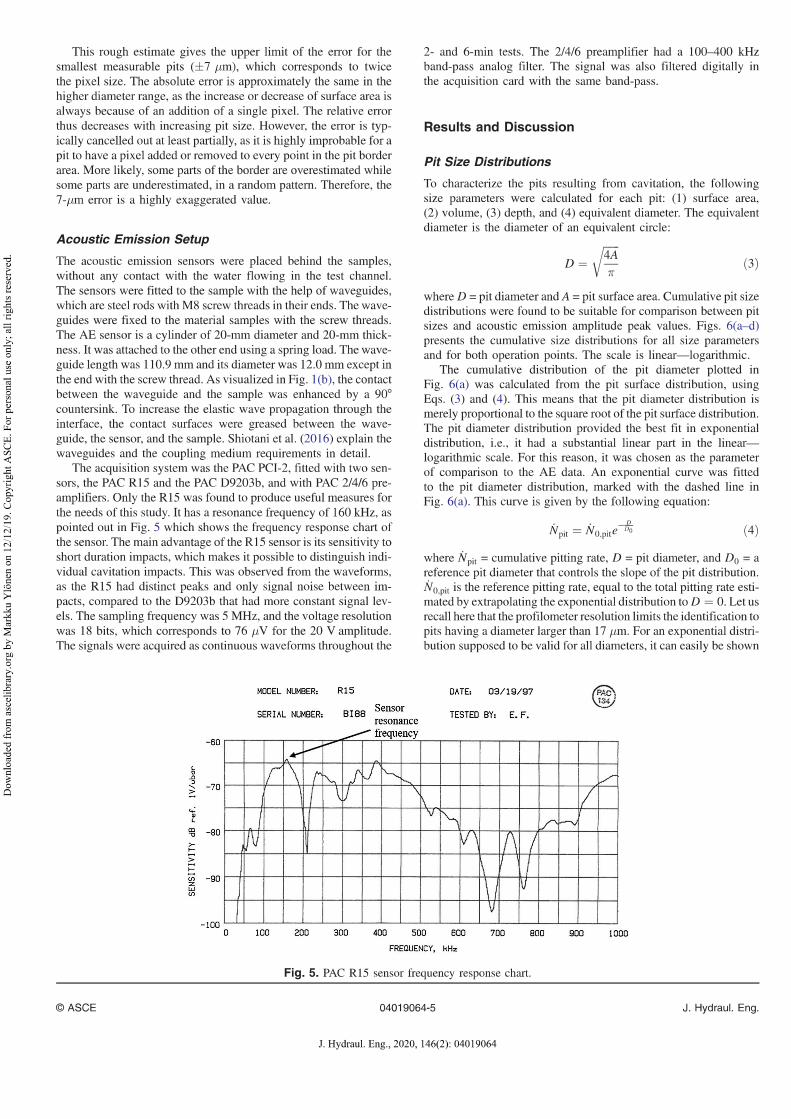
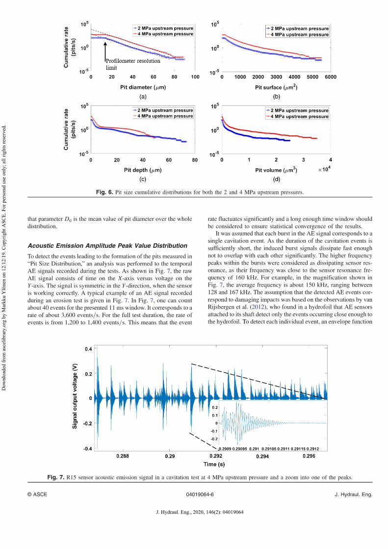
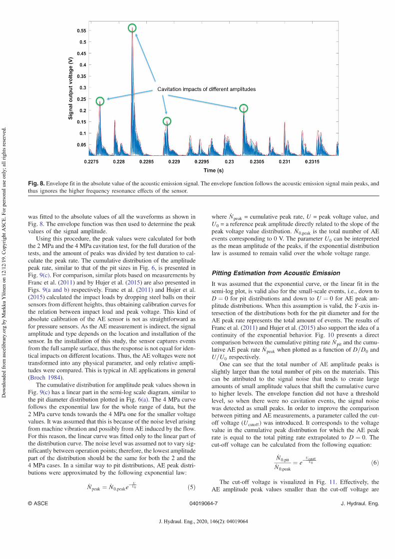
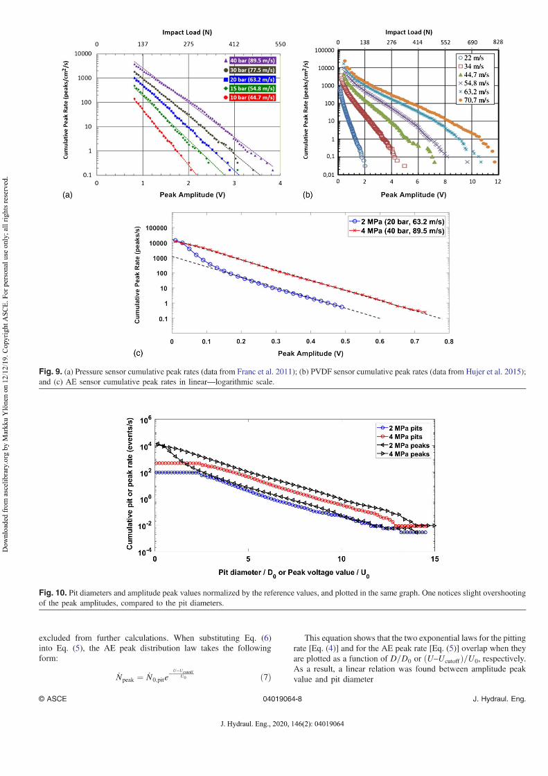
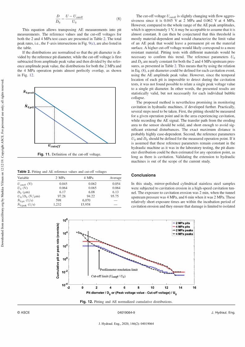
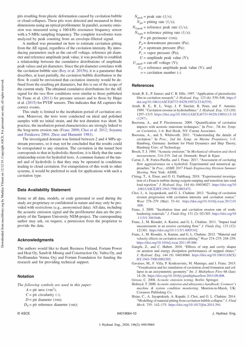
95

PUBLICATIONIV

Shedding Frequency in Cavitation E rosion E volution Tracking

Ylönen, Markku., Franc, Jean-Pierre., Miettinen, Juha., Saarenrinne, Pentti. & Fivel,Marc.

Journal of Multiphase Flow. 2019, Volume 118, p. 141-149.(https://doi.org/10.1016/j.ijmultiphaseflow.2019.06.009)

Publication reprinted with kind permission by

by E lsevier.

International Journal of Multiphase Flow 118 (2019) 141–149

Contents lists available at ScienceDirect

International Journal of Multiphase Flow

journal homepage: www.elsevier.com/locate/ijmulflow

Shedding frequency in cavitation erosion evolution tracking

Markku Ylönen a , ∗, Jean-Pierre Franc b , Juha Miettinen

a , Pentti Saarenrinne a , Marc Fivel c

a Tampere University, Faculty of Engineering and Natural Sciences, Korkeakoulunkatu 6, 33720 Tampere, Finland b Univ. Grenoble Alpes, CNRS, Grenoble INP, LEGI, 380 0 0 Grenoble, France c Univ. Grenoble Alpes, CNRS, Grenoble INP, SIMaP, 380 0 0 Grenoble, France

a r t i c l e i n f o

Article history:

Received 21 January 2019

Revised 6 May 2019

Accepted 12 June 2019

Available online 13 June 2019

Keywords:

Cavitation erosion

Cloud cavitation

Shedding frequency

Acoustic emission

a b s t r a c t

Cavitation erosion is a concern for most hydraulic machinery. An especially damaging type of cavitation

is cloud cavitation. This type of cavitation is characterized by a growth-collapse cycle in which a group

of vapor bubbles first grows together in a low-pressure region and then collapses almost simultaneously

when the pressure recovers. Measuring the frequency of these collapse events is possible by acoustic

emission (AE), as demonstrated in this study, in which a cavitation tunnel is utilized to create cloud cavi-

tation in the vicinity of a sample surface. These samples were equipped with AE sensors, and the initially

high frequency AE signal was demodulated to detect the relatively low frequency cloud cavitation shed-

ding. It was found that when the cavitation number is increased, AE successfully detects the changes in

this frequency, confirmed by comparing the results to video analysis and to simulations from literature.

Additionally, the frequency increases when cavitation erosion progresses, thus providing means to track

the erosion stage. It is concluded that the presented method is suitable for both detecting the transi-

tion from cloud to sheet cavitation and the erosion evolution in the experimental cavitation tunnel. The

method could probably be extended to non-intrusive hydraulic machine monitoring, as this type of cloud

cavitation is common in hydrofoils.

© 2019 Elsevier Ltd. All rights reserved.

1. Introduction

Cavitation is characterized by the growth and collapse of vapor

bubbles in a liquid. It can be observed either in a static liquid or

in a liquid flow due to decrease and the subsequent recovery of

the static pressure. The collapse of these bubbles potentially dam-

ages adjacent surfaces, as a result of the cumulated plasticity in-

duced at micrometer scale by each bubble collapse. Since the bub-

bles are typically quite numerous and the duration of exposure to

cavitation is generally long, damage tends to accumulate and reach

macroscopic levels. This causes serious harm to the structural in-

tegrity and flow performance of hydraulic machines, pipes, and

valves. This damage is typically difficult to avoid when searching

for the maximum benefit of an equipment at the expense of the

ideal conditions of use. Additionally, the extent of erosion is not

usually well known during operation, as it is difficult to monitor

in situ. Cavitation often occurs inside flow channels, where contin-

∗ Corresponding author.

E-mail addresses: markku.ylonen@tuni.fi (M. Ylönen),

jean-pierre.franc@legi.cnrs.fr (J.-P. Franc), juha.miettinen@tuni.fi (J. Miettinen),

pentti.saarenrinne@tuni.fi (P. Saarenrinne), marc.fivel@simap.grenoble-inp.fr (M.

Fivel).

uous visual observation may be difficult and costly, if not impossi-

ble.

This study focuses on cloud cavitation, which is a common type

of cavitation observed in various hydraulic equipment and in par-

ticular in hydrofoils. Cloud cavitation is a highly eroding type of

cavitation. A cloud of vapor bubbles forms in the leading edge of

a hydrofoil, due to an increase in the flow velocity, which leads to

the decrease in static pressure. It travels downstream the foil, and

collapses towards the trailing edge, if the static pressure recovers

sufficiently along the foil. The cloud is not static; it grows and col-

lapses periodically following a mechanism of growth, formation of

a re-entrant flow, shedding, and collapse. The shedding frequency

depends on flow velocity, surface quality, overall pressure, temper-

ature and surrounding liquid quality. ( Brennen et al., 20 0 0; Franc

and Michel, 2005; Nishimura et al., 2014; Gnanaskandan and Ma-

hesh, 2016; Hsiao et al., 2017 )

The current study can be divided into two main approaches in

detecting and utilizing the shedding frequency: (1) finding the cor-

relation between the cavitation number and the cloud shedding

frequency via acoustic emission (AE) and confirming the results

through comparison to high-speed video analysis and to simula-

tion results by other authors, and (2) tracking cavitation erosion

evolution through shedding frequency measured via AE. Material

samples that were fitted with AE sensors were eroded in a cavita-

https://doi.org/10.1016/j.ijmultiphaseflow.2019.06.009

0301-9322/© 2019 Elsevier Ltd. All rights reserved.

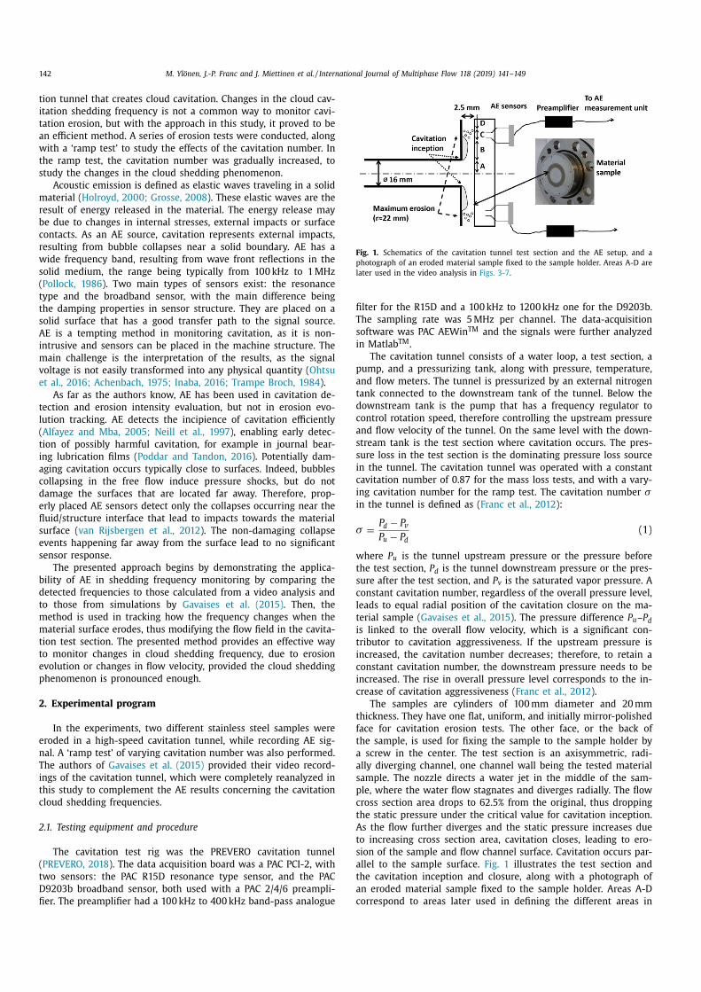
142 M. Ylönen, J.-P. Franc and J. Miettinen et al. / International Journal of Multiphase Flow 118 (2019) 141–149

tion tunnel that creates cloud cavitation. Changes in the cloud cav-

itation shedding frequency is not a common way to monitor cavi-

tation erosion, but with the approach in this study, it proved to be

an efficient method. A series of erosion tests were conducted, along

with a ‘ramp test’ to study the effects of the cavitation number. In

the ramp test, the cavitation number was gradually increased, to

study the changes in the cloud shedding phenomenon.

Acoustic emission is defined as elastic waves traveling in a solid

material ( Holroyd, 20 0 0; Grosse, 20 08 ). These elastic waves are the

result of energy released in the material. The energy release may

be due to changes in internal stresses, external impacts or surface

contacts. As an AE source, cavitation represents external impacts,

resulting from bubble collapses near a solid boundary. AE has a

wide frequency band, resulting from wave front reflections in the

solid medium, the range being typically from 100 kHz to 1 MHz

( Pollock, 1986 ). Two main types of sensors exist: the resonance

type and the broadband sensor, with the main difference being

the damping properties in sensor structure. They are placed on a

solid surface that has a good transfer path to the signal source.

AE is a tempting method in monitoring cavitation, as it is non-

intrusive and sensors can be placed in the machine structure. The

main challenge is the interpretation of the results, as the signal

voltage is not easily transformed into any physical quantity ( Ohtsu

et al., 2016; Achenbach, 1975; Inaba, 2016; Trampe Broch, 1984 ).

As far as the authors know, AE has been used in cavitation de-

tection and erosion intensity evaluation, but not in erosion evo-

lution tracking. AE detects the incipience of cavitation efficiently

( Alfayez and Mba, 2005; Neill et al., 1997 ), enabling early detec-

tion of possibly harmful cavitation, for example in journal bear-

ing lubrication films ( Poddar and Tandon, 2016 ). Potentially dam-

aging cavitation occurs typically close to surfaces. Indeed, bubbles

collapsing in the free flow induce pressure shocks, but do not

damage the surfaces that are located far away. Therefore, prop-

erly placed AE sensors detect only the collapses occurring near the

fluid/structure interface that lead to impacts towards the material

surface ( van Rijsbergen et al., 2012 ). The non-damaging collapse

events happening far away from the surface lead to no significant

sensor response.

The presented approach begins by demonstrating the applica-

bility of AE in shedding frequency monitoring by comparing the

detected frequencies to those calculated from a video analysis and

to those from simulations by Gavaises et al. (2015) . Then, the

method is used in tracking how the frequency changes when the

material surface erodes, thus modifying the flow field in the cavita-

tion test section. The presented method provides an effective way

to monitor changes in cloud shedding frequency, due to erosion

evolution or changes in flow velocity, provided the cloud shedding

phenomenon is pronounced enough.

2. Experimental program

In the experiments, two different stainless steel samples were

eroded in a high-speed cavitation tunnel, while recording AE sig-

nal. A ‘ramp test’ of varying cavitation number was also performed.

The authors of Gavaises et al. (2015) provided their video record-

ings of the cavitation tunnel, which were completely reanalyzed in

this study to complement the AE results concerning the cavitation

cloud shedding frequencies.

2.1. Testing equipment and procedure

The cavitation test rig was the PREVERO cavitation tunnel

( PREVERO, 2018 ). The data acquisition board was a PAC PCI-2, with

two sensors: the PAC R15D resonance type sensor, and the PAC

D9203b broadband sensor, both used with a PAC 2/4/6 preampli-

fier. The preamplifier had a 100 kHz to 400 kHz band-pass analogue

Fig. 1. Schematics of the cavitation tunnel test section and the AE setup, and a

photograph of an eroded material sample fixed to the sample holder. Areas A-D are

later used in the video analysis in Figs. 3-7 .

filter for the R15D and a 100 kHz to 1200 kHz one for the D9203b.

The sampling rate was 5 MHz per channel. The data-acquisition

software was PAC AEWin TM and the signals were further analyzed

in Matlab TM .

The cavitation tunnel consists of a water loop, a test section, a

pump, and a pressurizing tank, along with pressure, temperature,

and flow meters. The tunnel is pressurized by an external nitrogen

tank connected to the downstream tank of the tunnel. Below the

downstream tank is the pump that has a frequency regulator to

control rotation speed, therefore controlling the upstream pressure

and flow velocity of the tunnel. On the same level with the down-

stream tank is the test section where cavitation occurs. The pres-

sure loss in the test section is the dominating pressure loss source

in the tunnel. The cavitation tunnel was operated with a constant

cavitation number of 0.87 for the mass loss tests, and with a vary-

ing cavitation number for the ramp test. The cavitation number σ

in the tunnel is defined as ( Franc et al., 2012 ):

σ = P d − P v

P u − P d (1)

where P u is the tunnel upstream pressure or the pressure before

the test section, P d is the tunnel downstream pressure or the pres-

sure after the test section, and P v is the saturated vapor pressure. A

constant cavitation number, regardless of the overall pressure level,

leads to equal radial position of the cavitation closure on the ma-

terial sample ( Gavaises et al., 2015 ). The pressure difference P u –P d is linked to the overall flow velocity, which is a significant con-

tributor to cavitation aggressiveness. If the upstream pressure is

increased, the cavitation number decreases; therefore, to retain a

constant cavitation number, the downstream pressure needs to be

increased. The rise in overall pressure level corresponds to the in-

crease of cavitation aggressiveness ( Franc et al., 2012 ).

The samples are cylinders of 100 mm diameter and 20 mm

thickness. They have one flat, uniform, and initially mirror-polished

face for cavitation erosion tests. The other face, or the back of

the sample, is used for fixing the sample to the sample holder by

a screw in the center. The test section is an axisymmetric, radi-

ally diverging channel, one channel wall being the tested material

sample. The nozzle directs a water jet in the middle of the sam-

ple, where the water flow stagnates and diverges radially. The flow

cross section area drops to 62.5% from the original, thus dropping

the static pressure under the critical value for cavitation inception.

As the flow further diverges and the static pressure increases due

to increasing cross section area, cavitation closes, leading to ero-

sion of the sample and flow channel surface. Cavitation occurs par-

allel to the sample surface. Fig. 1 illustrates the test section and

the cavitation inception and closure, along with a photograph of

an eroded material sample fixed to the sample holder. Areas A-D

correspond to areas later used in defining the different areas in

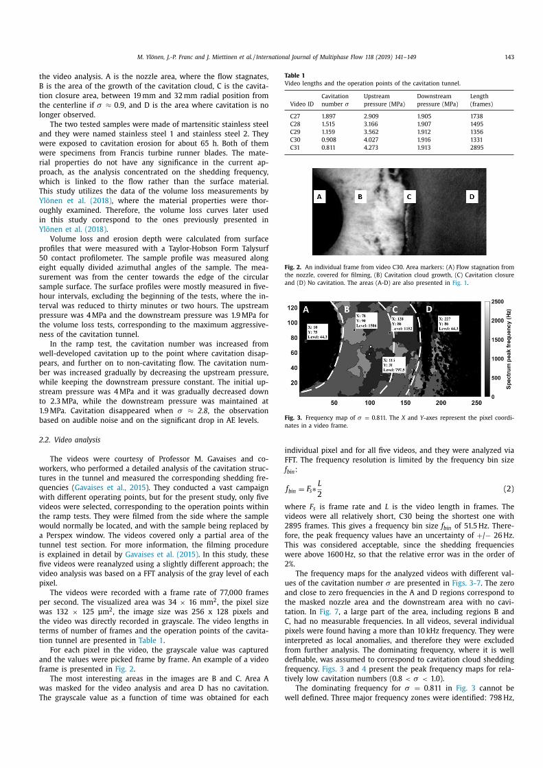
M. Ylönen, J.-P. Franc and J. Miettinen et al. / International Journal of Multiphase Flow 118 (2019) 141–149 143

the video analysis. A is the nozzle area, where the flow stagnates,

B is the area of the growth of the cavitation cloud, C is the cavita-

tion closure area, between 19 mm and 32 mm radial position from

the centerline if σ ≈ 0.9, and D is the area where cavitation is no

longer observed.

The two tested samples were made of martensitic stainless steel

and they were named stainless steel 1 and stainless steel 2. They

were exposed to cavitation erosion for about 65 h. Both of them

were specimens from Francis turbine runner blades. The mate-

rial properties do not have any significance in the current ap-

proach, as the analysis concentrated on the shedding frequency,

which is linked to the flow rather than the surface material.

This study utilizes the data of the volume loss measurements by

Ylönen et al. (2018) , where the material properties were thor-

oughly examined. Therefore, the volume loss curves later used

in this study correspond to the ones previously presented in

Ylönen et al. (2018) .

Volume loss and erosion depth were calculated from surface

profiles that were measured with a Taylor-Hobson Form Talysurf

50 contact profilometer. The sample profile was measured along

eight equally divided azimuthal angles of the sample. The mea-

surement was from the center towards the edge of the circular

sample surface. The surface profiles were mostly measured in five-

hour intervals, excluding the beginning of the tests, where the in-

terval was reduced to thirty minutes or two hours. The upstream

pressure was 4 MPa and the downstream pressure was 1.9 MPa for

the volume loss tests, corresponding to the maximum aggressive-

ness of the cavitation tunnel.

In the ramp test, the cavitation number was increased from

well-developed cavitation up to the point where cavitation disap-

pears, and further on to non-cavitating flow. The cavitation num-

ber was increased gradually by decreasing the upstream pressure,

while keeping the downstream pressure constant. The initial up-

stream pressure was 4 MPa and it was gradually decreased down

to 2.3 MPa, while the downstream pressure was maintained at

1.9 MPa. Cavitation disappeared when σ ≈ 2.8 , the observation

based on audible noise and on the significant drop in AE levels.

2.2. Video analysis

The videos were courtesy of Professor M. Gavaises and co-

workers, who performed a detailed analysis of the cavitation struc-

tures in the tunnel and measured the corresponding shedding fre-

quencies ( Gavaises et al., 2015 ). They conducted a vast campaign

with different operating points, but for the present study, only five

videos were selected, corresponding to the operation points within

the ramp tests. They were filmed from the side where the sample

would normally be located, and with the sample being replaced by

a Perspex window. The videos covered only a partial area of the

tunnel test section. For more information, the filming procedure

is explained in detail by Gavaises et al. (2015) . In this study, these

five videos were reanalyzed using a slightly different approach; the

video analysis was based on a FFT analysis of the gray level of each

pixel.

The videos were recorded with a frame rate of 77,0 0 0 frames

per second. The visualized area was 34 × 16 mm 2 , the pixel size

was 132 × 125 μm 2 , the image size was 256 x 128 pixels and

the video was directly recorded in grayscale. The video lengths in

terms of number of frames and the operation points of the cavita-

tion tunnel are presented in Table 1 .

For each pixel in the video, the grayscale value was captured

and the values were picked frame by frame. An example of a video

frame is presented in Fig. 2 .

The most interesting areas in the images are B and C. Area A

was masked for the video analysis and area D has no cavitation.

The grayscale value as a function of time was obtained for each

Table 1

Video lengths and the operation points of the cavitation tunnel.

Video ID

Cavitation

number σ

Upstream

pressure (MPa)

Downstream

pressure (MPa)

Length

(frames)

C27 1.897 2.909 1.905 1738

C28 1.515 3.166 1.907 1495

C29 1.159 3.562 1.912 1356

C30 0.908 4.027 1.916 1331

C31 0.811 4.273 1.913 2895

Fig. 2. An individual frame from video C30. Area markers: (A) Flow stagnation from

the nozzle, covered for filming, (B) Cavitation cloud growth, (C) Cavitation closure

and (D) No cavitation. The areas (A-D) are also presented in Fig. 1 .

Fig. 3. Frequency map of σ = 0.811. The X and Y -axes represent the pixel coordi-

nates in a video frame.

individual pixel and for all five videos, and they were analyzed via

FFT. The frequency resolution is limited by the frequency bin size

f bin :

f bin = F s ∗L

2 (2)

where F s is frame rate and L is the video length in frames. The

videos were all relatively short, C30 being the shortest one with

2895 frames. This gives a frequency bin size f bin of 51.5 Hz. There-

fore, the peak frequency values have an uncertainty of + / − 26 Hz.

This was considered acceptable, since the shedding frequencies

were above 1600 Hz, so that the relative error was in the order of

2%.

The frequency maps for the analyzed videos with different val-

ues of the cavitation number σ are presented in Figs. 3-7 . The zero

and close to zero frequencies in the A and D regions correspond to

the masked nozzle area and the downstream area with no cavi-

tation. In Fig. 7 , a large part of the area, including regions B and

C, had no measurable frequencies. In all videos, several individual

pixels were found having a more than 10 kHz frequency. They were

interpreted as local anomalies, and therefore they were excluded

from further analysis. The dominating frequency, where it is well

definable, was assumed to correspond to cavitation cloud shedding

frequency. Figs. 3 and 4 present the peak frequency maps for rela-

tively low cavitation numbers (0.8 < σ < 1.0).

The dominating frequency for σ = 0.811 in Fig. 3 cannot be

well defined. Three major frequency zones were identified: 798 Hz,

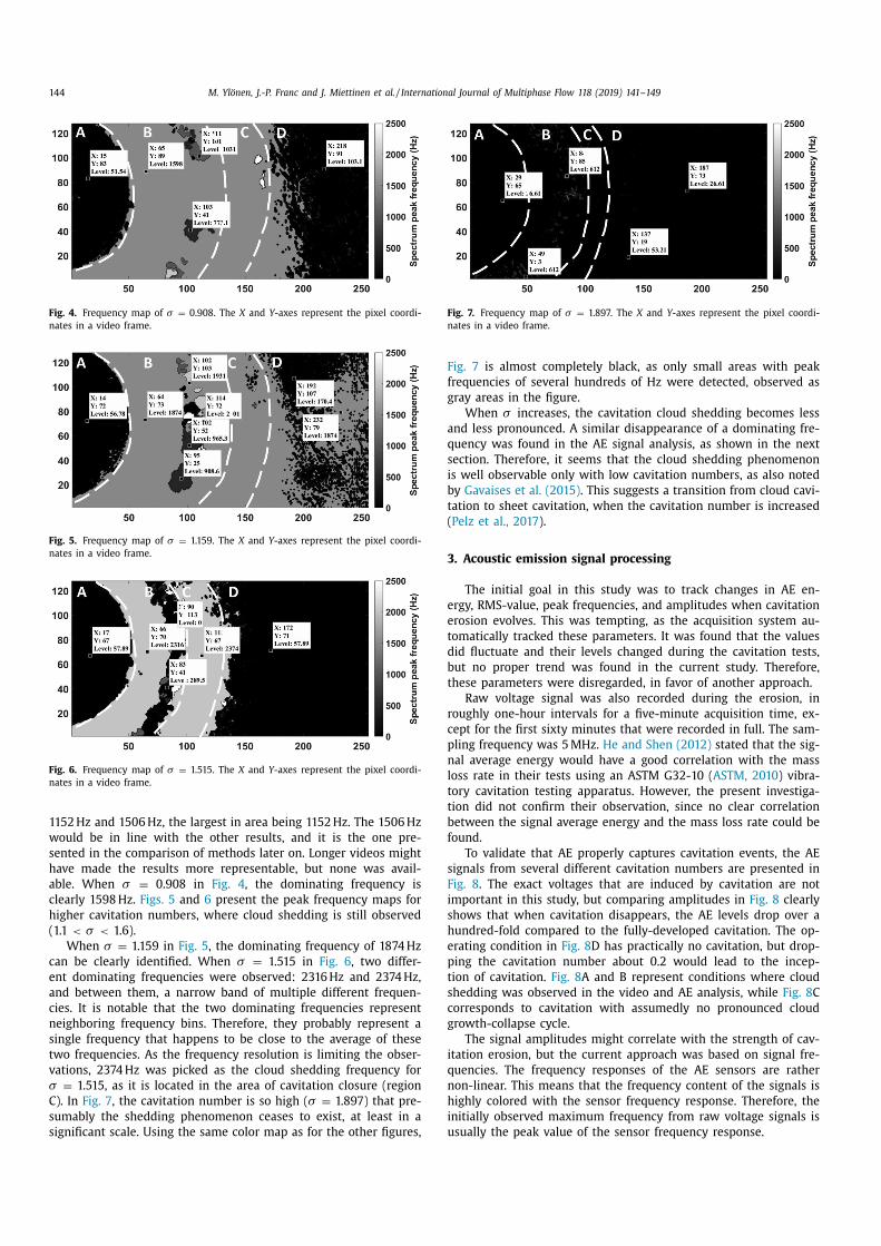
144 M. Ylönen, J.-P. Franc and J. Miettinen et al. / International Journal of Multiphase Flow 118 (2019) 141–149

Fig. 4. Frequency map of σ = 0.908. The X and Y -axes represent the pixel coordi-

nates in a video frame.

Fig. 5. Frequency map of σ = 1.159. The X and Y -axes represent the pixel coordi-

nates in a video frame.

Fig. 6. Frequency map of σ = 1.515. The X and Y -axes represent the pixel coordi-

nates in a video frame.

1152 Hz and 1506 Hz, the largest in area being 1152 Hz. The 1506 Hz

would be in line with the other results, and it is the one pre-

sented in the comparison of methods later on. Longer videos might

have made the results more representable, but none was avail-

able. When σ = 0.908 in Fig. 4 , the dominating frequency is

clearly 1598 Hz. Figs. 5 and 6 present the peak frequency maps for

higher cavitation numbers, where cloud shedding is still observed

(1.1 < σ < 1.6).

When σ = 1.159 in Fig. 5 , the dominating frequency of 1874 Hz

can be clearly identified. When σ = 1.515 in Fig. 6 , two differ-

ent dominating frequencies were observed: 2316 Hz and 2374 Hz,

and between them, a narrow band of multiple different frequen-

cies. It is notable that the two dominating frequencies represent

neighboring frequency bins. Therefore, they probably represent a

single frequency that happens to be close to the average of these

two frequencies. As the frequency resolution is limiting the obser-

vations, 2374 Hz was picked as the cloud shedding frequency for

σ = 1.515, as it is located in the area of cavitation closure (region

C). In Fig. 7 , the cavitation number is so high ( σ = 1.897) that pre-

sumably the shedding phenomenon ceases to exist, at least in a

significant scale. Using the same color map as for the other figures,

Fig. 7. Frequency map of σ = 1.897. The X and Y -axes represent the pixel coordi-

nates in a video frame.

Fig. 7 is almost completely black, as only small areas with peak

frequencies of several hundreds of Hz were detected, observed as

gray areas in the figure.

When σ increases, the cavitation cloud shedding becomes less

and less pronounced. A similar disappearance of a dominating fre-

quency was found in the AE signal analysis, as shown in the next

section. Therefore, it seems that the cloud shedding phenomenon

is well observable only with low cavitation numbers, as also noted

by Gavaises et al. (2015) . This suggests a transition from cloud cavi-

tation to sheet cavitation, when the cavitation number is increased

( Pelz et al., 2017 ).

3. Acoustic emission signal processing

The initial goal in this study was to track changes in AE en-

ergy, RMS-value, peak frequencies, and amplitudes when cavitation

erosion evolves. This was tempting, as the acquisition system au-

tomatically tracked these parameters. It was found that the values

did fluctuate and their levels changed during the cavitation tests,

but no proper trend was found in the current study. Therefore,

these parameters were disregarded, in favor of another approach.

Raw voltage signal was also recorded during the erosion, in

roughly one-hour intervals for a five-minute acquisition time, ex-

cept for the first sixty minutes that were recorded in full. The sam-

pling frequency was 5 MHz. He and Shen (2012) stated that the sig-

nal average energy would have a good correlation with the mass

loss rate in their tests using an ASTM G32-10 ( ASTM, 2010 ) vibra-

tory cavitation testing apparatus. However, the present investiga-

tion did not confirm their observation, since no clear correlation

between the signal average energy and the mass loss rate could be

found.

To validate that AE properly captures cavitation events, the AE

signals from several different cavitation numbers are presented in

Fig. 8 . The exact voltages that are induced by cavitation are not

important in this study, but comparing amplitudes in Fig. 8 clearly

shows that when cavitation disappears, the AE levels drop over a

hundred-fold compared to the fully-developed cavitation. The op-

erating condition in Fig. 8 D has practically no cavitation, but drop-

ping the cavitation number about 0.2 would lead to the incep-

tion of cavitation. Fig. 8 A and B represent conditions where cloud

shedding was observed in the video and AE analysis, while Fig. 8 C

corresponds to cavitation with assumedly no pronounced cloud

growth-collapse cycle.

The signal amplitudes might correlate with the strength of cav-

itation erosion, but the current approach was based on signal fre-

quencies. The frequency responses of the AE sensors are rather

non-linear. This means that the frequency content of the signals is

highly colored with the sensor frequency response. Therefore, the

initially observed maximum frequency from raw voltage signals is

usually the peak value of the sensor frequency response.

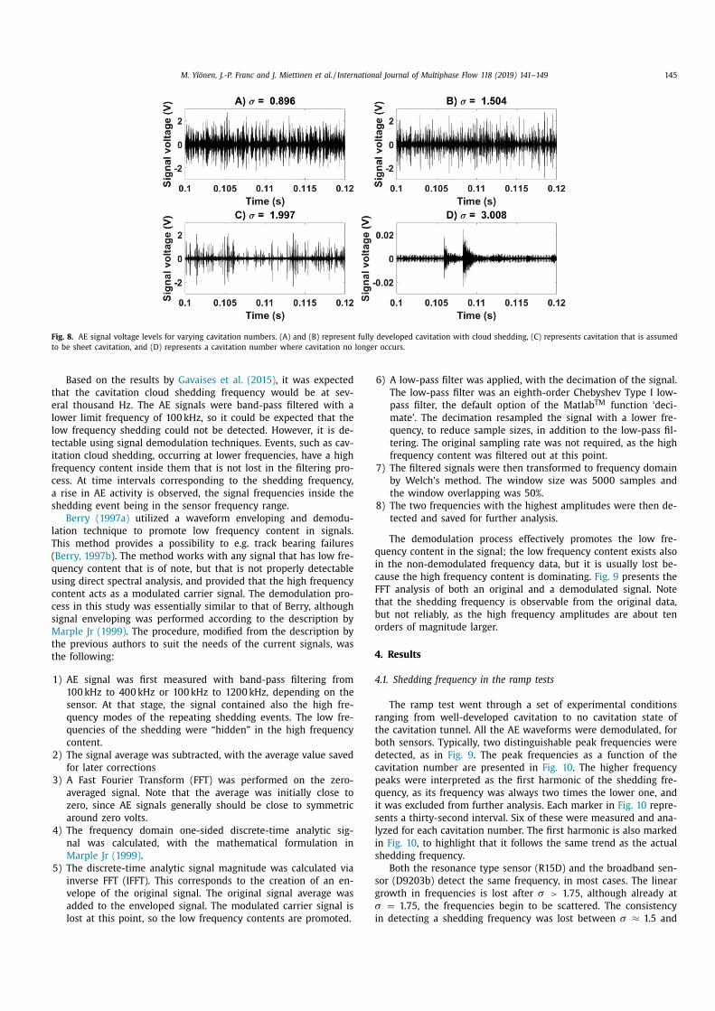
M. Ylönen, J.-P. Franc and J. Miettinen et al. / International Journal of Multiphase Flow 118 (2019) 141–149 145

Fig. 8. AE signal voltage levels for varying cavitation numbers. (A) and (B) represent fully developed cavitation with cloud shedding, (C) represents cavitation that is assumed

to be sheet cavitation, and (D) represents a cavitation number where cavitation no longer occurs.

Based on the results by Gavaises et al. (2015) , it was expected

that the cavitation cloud shedding frequency would be at sev-

eral thousand Hz. The AE signals were band-pass filtered with a

lower limit frequency of 100 kHz, so it could be expected that the

low frequency shedding could not be detected. However, it is de-

tectable using signal demodulation techniques. Events, such as cav-

itation cloud shedding, occurring at lower frequencies, have a high

frequency content inside them that is not lost in the filtering pro-

cess. At time intervals corresponding to the shedding frequency,

a rise in AE activity is observed, the signal frequencies inside the

shedding event being in the sensor frequency range.

Berry (1997a) utilized a waveform enveloping and demodu-

lation technique to promote low frequency content in signals.

This method provides a possibility to e.g. track bearing failures

( Berry, 1997b ). The method works with any signal that has low fre-

quency content that is of note, but that is not properly detectable

using direct spectral analysis, and provided that the high frequency

content acts as a modulated carrier signal. The demodulation pro-

cess in this study was essentially similar to that of Berry, although

signal enveloping was performed according to the description by

Marple Jr (1999) . The procedure, modified from the description by

the previous authors to suit the needs of the current signals, was

the following:

1) AE signal was first measured with band-pass filtering from

10 0 kHz to 40 0 kHz or 10 0 kHz to 120 0 kHz, depending on the

sensor. At that stage, the signal contained also the high fre-

quency modes of the repeating shedding events. The low fre-

quencies of the shedding were “hidden” in the high frequency

content.

2) The signal average was subtracted, with the average value saved

for later corrections

3) A Fast Fourier Transform (FFT) was performed on the zero-

averaged signal. Note that the average was initially close to

zero, since AE signals generally should be close to symmetric

around zero volts.

4) The frequency domain one-sided discrete-time analytic sig-

nal was calculated, with the mathematical formulation in

Marple Jr (1999) .

5) The discrete-time analytic signal magnitude was calculated via

inverse FFT (IFFT). This corresponds to the creation of an en-

velope of the original signal. The original signal average was

added to the enveloped signal. The modulated carrier signal is

lost at this point, so the low frequency contents are promoted.

6) A low-pass filter was applied, with the decimation of the signal.

The low-pass filter was an eighth-order Chebyshev Type I low-

pass filter, the default option of the Matlab TM function ‘deci-

mate’. The decimation resampled the signal with a lower fre-

quency, to reduce sample sizes, in addition to the low-pass fil-

tering. The original sampling rate was not required, as the high

frequency content was filtered out at this point.

7) The filtered signals were then transformed to frequency domain

by Welch’s method. The window size was 50 0 0 samples and

the window overlapping was 50%.

8) The two frequencies with the highest amplitudes were then de-

tected and saved for further analysis.

The demodulation process effectively promotes the low fre-

quency content in the signal; the low frequency content exists also

in the non-demodulated frequency data, but it is usually lost be-

cause the high frequency content is dominating. Fig. 9 presents the

FFT analysis of both an original and a demodulated signal. Note

that the shedding frequency is observable from the original data,

but not reliably, as the high frequency amplitudes are about ten

orders of magnitude larger.

4. Results

4.1. Shedding frequency in the ramp tests

The ramp test went through a set of experimental conditions

ranging from well-developed cavitation to no cavitation state of

the cavitation tunnel. All the AE waveforms were demodulated, for

both sensors. Typically, two distinguishable peak frequencies were

detected, as in Fig. 9 . The peak frequencies as a function of the

cavitation number are presented in Fig. 10 . The higher frequency

peaks were interpreted as the first harmonic of the shedding fre-

quency, as its frequency was always two times the lower one, and

it was excluded from further analysis. Each marker in Fig. 10 repre-

sents a thirty-second interval. Six of these were measured and ana-

lyzed for each cavitation number. The first harmonic is also marked

in Fig. 10 , to highlight that it follows the same trend as the actual

shedding frequency.

Both the resonance type sensor (R15D) and the broadband sen-

sor (D9203b) detect the same frequency, in most cases. The linear

growth in frequencies is lost after σ > 1.75, although already at

σ = 1.75, the frequencies begin to be scattered. The consistency

in detecting a shedding frequency was lost between σ ≈ 1.5 and

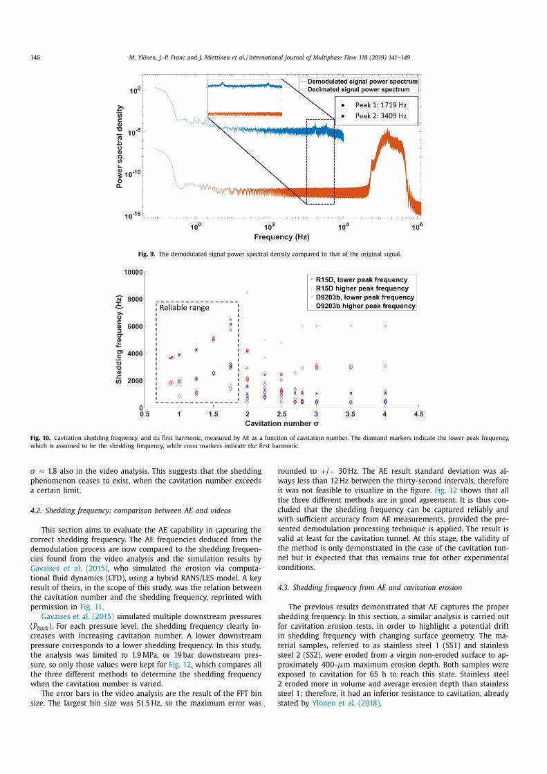
146 M. Ylönen, J.-P. Franc and J. Miettinen et al. / International Journal of Multiphase Flow 118 (2019) 141–149

Fig. 9. The demodulated signal power spectral density compared to that of the original signal.

Fig. 10. Cavitation shedding frequency, and its first harmonic, measured by AE as a function of cavitation number. The diamond markers indicate the lower peak frequency,

which is assumed to be the shedding frequency, while cross markers indicate the first harmonic.

σ ≈ 1.8 also in the video analysis. This suggests that the shedding

phenomenon ceases to exist, when the cavitation number exceeds

a certain limit.

4.2. Shedding frequency: comparison between AE and videos

This section aims to evaluate the AE capability in capturing the

correct shedding frequency. The AE frequencies deduced from the

demodulation process are now compared to the shedding frequen-

cies found from the video analysis and the simulation results by

Gavaises et al. (2015) , who simulated the erosion via computa-

tional fluid dynamics (CFD), using a hybrid RANS/LES model. A key

result of theirs, in the scope of this study, was the relation between

the cavitation number and the shedding frequency, reprinted with

permission in Fig. 11 .

Gavaises et al. (2015) simulated multiple downstream pressures

( P back ). For each pressure level, the shedding frequency clearly in-

creases with increasing cavitation number. A lower downstream

pressure corresponds to a lower shedding frequency. In this study,

the analysis was limited to 1.9 MPa, or 19 bar downstream pres-

sure, so only those values were kept for Fig. 12 , which compares all

the three different methods to determine the shedding frequency

when the cavitation number is varied.

The error bars in the video analysis are the result of the FFT bin

size. The largest bin size was 51.5 Hz, so the maximum error was

rounded to + / − 30 Hz. The AE result standard deviation was al-

ways less than 12 Hz between the thirty-second intervals, therefore

it was not feasible to visualize in the figure. Fig. 12 shows that all

the three different methods are in good agreement. It is thus con-

cluded that the shedding frequency can be captured reliably and

with sufficient accuracy from AE measurements, provided the pre-

sented demodulation processing technique is applied. The result is

valid at least for the cavitation tunnel. At this stage, the validity of

the method is only demonstrated in the case of the cavitation tun-

nel but is expected that this remains true for other experimental

conditions.

4.3. Shedding frequency from AE and cavitation erosion

The previous results demonstrated that AE captures the proper

shedding frequency. In this section, a similar analysis is carried out

for cavitation erosion tests, in order to highlight a potential drift

in shedding frequency with changing surface geometry. The ma-

terial samples, referred to as stainless steel 1 (SS1) and stainless

steel 2 (SS2), were eroded from a virgin non-eroded surface to ap-

proximately 400- µm maximum erosion depth. Both samples were

exposed to cavitation for 65 h to reach this state. Stainless steel

2 eroded more in volume and average erosion depth than stainless

steel 1; therefore, it had an inferior resistance to cavitation, already

stated by Ylönen et al. (2018) .

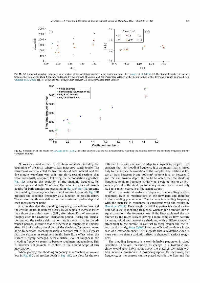
M. Ylönen, J.-P. Franc and J. Miettinen et al. / International Journal of Multiphase Flow 118 (2019) 141–149 147

Fig. 11. (a) Simulated shedding frequency as a function of the cavitation number in the cavitation tunnel by Gavaises et al. (2015) . (b) The Strouhal number St was de-

fined as the ratio of shedding frequency multiplied by the gap size of 2.5 mm and the mean flow velocity at the 25 mm radius of the diverging channel. Reprinted from

Gavaises et al. (2015) , Fig. 15, Copyright 0301-9322/© 2014 Elsevier Ltd, with permission from Elsevier.

Fig. 12. Comparison of the results by Gavaises et al. (2015) , the video analysis, and the AE measurements, regarding the relation between the shedding frequency and the

cavitation number.

AE was measured at one- to two-hour intervals, excluding the

beginning of the tests, where it was measured continuously. The

waveforms were collected for five minutes at each interval, and the

five-minute waveform was split into thirty-second sections that

were individually analyzed, following the demodulation algorithm.

Fig. 13 A presents the evolution of the shedding frequency, for

both samples and both AE sensors. The volume losses and erosion

depths for both samples are presented in Fig. 13 B. Fig. 13 C presents

the shedding frequency as a function of volume loss, while Fig. 13 D

presents the shedding frequency as a function of erosion depth.

The erosion depth was defined as the maximum profile depth at

each measurement point.

It is notable that the shedding frequency, the volume loss and

the erosion depth of stainless steel 2 (SS2) begins to increase faster

than those of stainless steel 1 (SS1), after about 12 h of erosion, or

roughly after the cavitation incubation period. During the incuba-

tion period, the surface deformation rate is slower than in the ad-

vanced periods, meaning that the increase in roughness is smaller.

After 48 h of erosion, the slopes of the shedding frequency curves

begin to decrease, reaching possibly a constant value. This suggests

that the changes in roughness might have little effect when the

surface is highly damaged. After a critical level of roughness, the

shedding frequency seems to become roughness independent. This

is, however, not possible to confirm in the limited scope of this

investigation.

When plotting the shedding frequency as a function of volume

loss in Fig. 13 C and erosion depth in Fig. 13 D, the plots for the two

different tests and materials overlap to a significant degree. This

suggests that the shedding frequency is a parameter that is linked

only to the surface deformation of the samples. The relation is lin-

ear at least between 0 and 100 mm 3 volume loss, or between 0

and 350 µm erosion depth. It should be noted that the shedding

frequency tends to fluctuate, so deriving a volume loss or an ero-

sion depth out of the shedding frequency measurement would only

lead to a rough estimate of the actual values.

When the material surface is degraded, the resulting surface

roughness leads to modifications in the flow field and therefore

in the shedding phenomenon. The increase in shedding frequency

with the increase in roughness is consistent with the results by

Hao et al. (2017) . Their rough hydrofoil experiencing cloud cavita-

tion had a 20 Hz shedding frequency, whereas for a smooth one in

equal conditions, the frequency was 17 Hz. They explained the dif-

ference by the rough surface having a more complex flow pattern,

including initial and large-scale shedding, with a different type of

attachment to the surface. In contrast to these results and the re-

sults in this study, Stutz (2003) found no effect of roughness in the

case of a cavitation sheet. This suggests that a cavitation cloud is

more sensitive than a cavitation sheet to changes in surface rough-

ness.

The shedding frequency is a well-definable parameter in cloud

cavitation. Therefore, measuring its change in a hydraulic ma-

chine would give information about the state of cavitation ero-

sion. Acoustic emission is a promising option for measuring the

frequency, as the sensors can be placed outside the flow and the

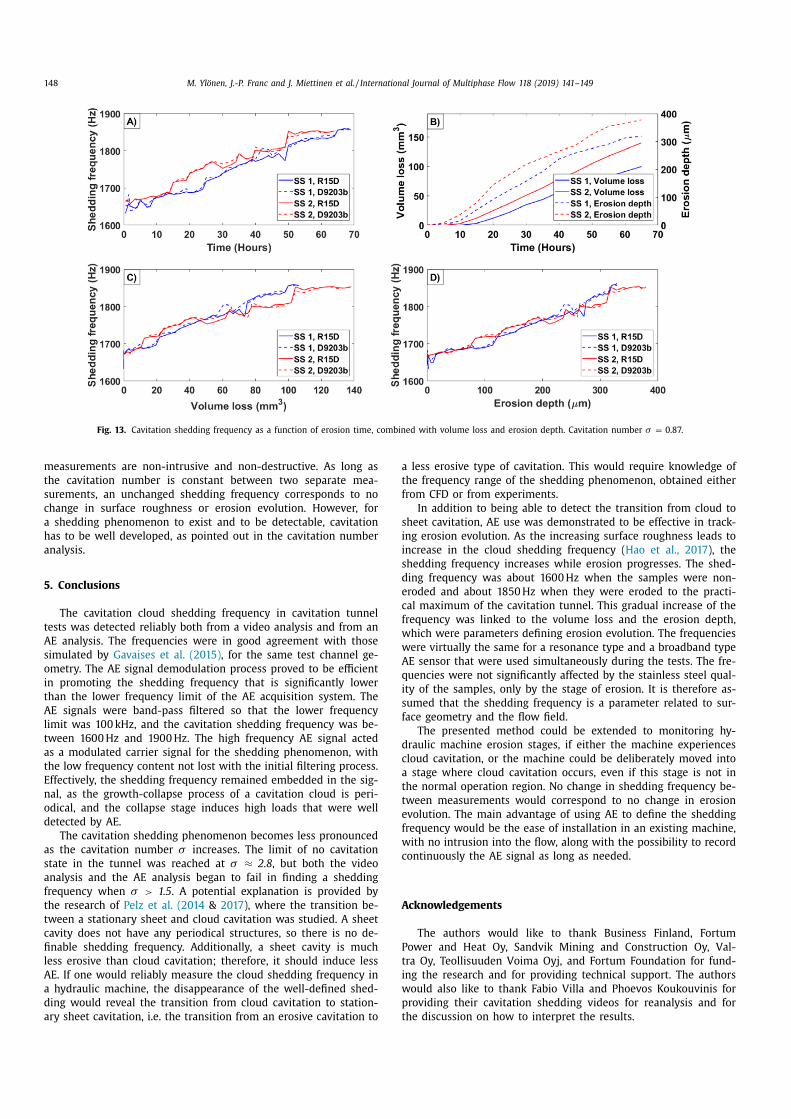
148 M. Ylönen, J.-P. Franc and J. Miettinen et al. / International Journal of Multiphase Flow 118 (2019) 141–149

Fig. 13. Cavitation shedding frequency as a function of erosion time, combined with volume loss and erosion depth. Cavitation number σ = 0.87.

measurements are non-intrusive and non-destructive. As long as

the cavitation number is constant between two separate mea-

surements, an unchanged shedding frequency corresponds to no

change in surface roughness or erosion evolution. However, for

a shedding phenomenon to exist and to be detectable, cavitation

has to be well developed, as pointed out in the cavitation number

analysis.

5. Conclusions

The cavitation cloud shedding frequency in cavitation tunnel

tests was detected reliably both from a video analysis and from an

AE analysis. The frequencies were in good agreement with those

simulated by Gavaises et al. (2015) , for the same test channel ge-

ometry. The AE signal demodulation process proved to be efficient

in promoting the shedding frequency that is significantly lower

than the lower frequency limit of the AE acquisition system. The

AE signals were band-pass filtered so that the lower frequency

limit was 100 kHz, and the cavitation shedding frequency was be-

tween 1600 Hz and 1900 Hz. The high frequency AE signal acted

as a modulated carrier signal for the shedding phenomenon, with

the low frequency content not lost with the initial filtering process.

Effectively, the shedding frequency remained embedded in the sig-

nal, as the growth-collapse process of a cavitation cloud is peri-

odical, and the collapse stage induces high loads that were well

detected by AE.

The cavitation shedding phenomenon becomes less pronounced

as the cavitation number σ increases. The limit of no cavitation

state in the tunnel was reached at σ ≈ 2.8 , but both the video

analysis and the AE analysis began to fail in finding a shedding

frequency when σ > 1.5 . A potential explanation is provided by

the research of Pelz et al. (2014 & 2017 ), where the transition be-

tween a stationary sheet and cloud cavitation was studied. A sheet

cavity does not have any periodical structures, so there is no de-

finable shedding frequency. Additionally, a sheet cavity is much

less erosive than cloud cavitation; therefore, it should induce less

AE. If one would reliably measure the cloud shedding frequency in

a hydraulic machine, the disappearance of the well-defined shed-

ding would reveal the transition from cloud cavitation to station-

ary sheet cavitation, i.e. the transition from an erosive cavitation to

a less erosive type of cavitation. This would require knowledge of

the frequency range of the shedding phenomenon, obtained either

from CFD or from experiments.

In addition to being able to detect the transition from cloud to

sheet cavitation, AE use was demonstrated to be effective in track-

ing erosion evolution. As the increasing surface roughness leads to

increase in the cloud shedding frequency ( Hao et al., 2017 ), the

shedding frequency increases while erosion progresses. The shed-

ding frequency was about 1600 Hz when the samples were non-

eroded and about 1850 Hz when they were eroded to the practi-

cal maximum of the cavitation tunnel. This gradual increase of the

frequency was linked to the volume loss and the erosion depth,

which were parameters defining erosion evolution. The frequencies

were virtually the same for a resonance type and a broadband type

AE sensor that were used simultaneously during the tests. The fre-

quencies were not significantly affected by the stainless steel qual-

ity of the samples, only by the stage of erosion. It is therefore as-

sumed that the shedding frequency is a parameter related to sur-

face geometry and the flow field.

The presented method could be extended to monitoring hy-

draulic machine erosion stages, if either the machine experiences

cloud cavitation, or the machine could be deliberately moved into

a stage where cloud cavitation occurs, even if this stage is not in

the normal operation region. No change in shedding frequency be-

tween measurements would correspond to no change in erosion

evolution. The main advantage of using AE to define the shedding

frequency would be the ease of installation in an existing machine,

with no intrusion into the flow, along with the possibility to record

continuously the AE signal as long as needed.

Acknowledgements

The authors would like to thank Business Finland, Fortum

Power and Heat Oy, Sandvik Mining and Construction Oy, Val-

tra Oy, Teollisuuden Voima Oyj, and Fortum Foundation for fund-

ing the research and for providing technical support. The authors

would also like to thank Fabio Villa and Phoevos Koukouvinis for

providing their cavitation shedding videos for reanalysis and for

the discussion on how to interpret the results.

M. Ylönen, J.-P. Franc and J. Miettinen et al. / International Journal of Multiphase Flow 118 (2019) 141–149 149

Supplementary materials

Supplementary material associated with this article can be

found, in the online version, at doi: 10.1016/j.ijmultiphaseflow.2019.

06.009 .

References

Achenbach, J.D. , 1975. Wave Propagation in Elastic Solids. North Holland Publishing . Alfayez, L. , Mba, D. , 2005. Detection of incipient cavitation and determination of the

best efficiency point for centrifugal pumps using acoustic emission. Proc. Inst. Mech. Eng. Part E 219 (4), 327–344 .

ASTM International, 2010. ASTM G32-10, Standard Test Method for Cavitation Ero- sion Using Vibratory Apparatus .

Berry, J.E. , 1997a. High Frequency Enveloping and Demodulation Techniques Using Instruments From Various Vendors. Technical Associates of Charlotte, P.C .

Berry, J.E. , 1997b. Tracking of Rolling Element Bearing Failure Stages Using Both Vi-

bration Signature Analysis as Well as High Frequency Envelopping and Demod- ulation Special Techniques. Technical Associates of Charlotte, P.C .

Brennen, C. , Colonius, Y. , Wang, A. , Preston, A. , 20 0 0. Cloud cavitation phenomena. In: Twenty-Second Symposium on Naval Hydrodynamics, pp. 239–253 .

Franc, J. , Michel, J. , 2005. Fundamentals of Cavitation. Springer Science + Business Media, Inc. .

Franc, J. , Riondet, M. , Karimi, A. , Chahine, G.L. , 2012. Material and velocity effects on

cavitation erosion pitting. Wear 274–275, 248–259 . Gavaises, M. , Villa, F. , Koukouvinis, P. , Marengo, M. , Franc, J. , 2015. Visualisation and

les simulation of cavitation cloud formation and collapse in an axisymmetric geometry. Int. J. Multiph. Flow 68, 14–26 .

Gnanaskandan, A. , Mahesh, K. , 2016. Large eddy simulation of the transition from sheet to cloud cavitation over a wedge. Int. J. Multiph. Flow 83, 86–102 .

Grosse, C. , 2008. Acoustic Emission Testing. Springer Berlin Heidelberg, Heidelberg,

Germany . Hao, J. , Zhang, M. , Huang, X. , 2017. The influence of surface roughness on cloud

cavitation flow around hydrofoils. Acta Mech. Sin. 34 (1), 10–21 . He, Y. , Shen, Z. , 2012. Experimental research on cavitation erosion detection based

on acoustic emission technique. In: 30th European Conference on Acoustic Emission Testing & 7th International Conference on Acoustic Emission, pp. 1–8 .

Holroyd, T. , 20 0 0. Acoustic Emission and Ultrasonics Handbook (Coxmoor’s Machine

& System Condition Monitoring). Coxmoor Publishing Co., Moreton-in-Marsh, United Kingdom .

Hsiao, C. , Ma, J. , Chahine, G.L. , 2017. Multiscale tow-phase flow modeling of sheet and cloud cavitation. Int. J. Multiph. Flow 90, 102–117 .

Inaba, H. , 2016. AE sensor (AE Transducer), practical acoustic emission testing. Jpn. Soc. Non-Destruct. Insp. 35–45 .

Marple Jr, L. , 1999. Computing the discrete-time "analytic" signal via FFT. IEEE Trans. Signal Process. 47, 2600–2603 .

Neill, G.D. , Reuben, R.L. , Sandford, P.M. , Brown, E.R. , Steel, J.A. , 1997. Detection of incipient cavitation in pumps using acoustic emission. Proc. Ins. Mech. Eng. 211

(4), 267–277 .

Nishimura, S. , Takakuwa, O. , Soyama, H. , 2014. Effect of nozzle geometry on aggres- sivity of cavitating jet for cavitation erosion test and applications. In: Kim, K.,

Chahine, G., Franc, J., Karimi, A. (Eds.), Advanced Experimental and Numerical Techniques For Cavitation Erosion Prediction. Springer, Netherlands, Dordrecht,

pp. 283–302 . Ohtsu, M. , Enoki, M. , Mizutani, Y. , Shigeishi, M. , 2016. Principles of the acoustic

emission (AE) method and signal processing, practical acoustic emission test-

ing. Jpn. Soc. Non-Destruct. Insp. 5–35 . Pelz, P. , Keil, T. , Groß, T. , 2017. The transition from sheet to cloud cavitation. J. Fluid

Mech. 817, 439–454 . Pelz, P. , Keil, T. , Ludwig, G. , 2014. On the kinematics of sheet and cloud cavitation

and related erosion. Fluid Mech. Appl. 106, 221–237 . Poddar, S. , Tandon, N. , 2016. Detection of journal bearing vapour cavitation using

vibration and acoustic emission techniques with the aid of oil film photography.

Tribol. Int. 103, 95–101 . Pollock, A .A . , 1986. Classical wave theory in practical AE testing. In: Progress in

Acoustic Emission III: proceedings of the 8th International Acoustic Emission Symposium, pp. 708–722 .

PREVERO, 2018. The PREVERO Cavitation Erosion Tunnel http://web.archive. org/web/20180327065723/http://www.legi.grenoble-inp.fr/web/spip.php?

article1265&lang=fr .

Stutz, B. , 2003. Influence of roughness on the two-phase flow structure of sheet cavitation. J. Fluids Eng. 125 (4), 652–659 .

Trampe Broch, J. , 1984. Acoustic Emission, Mechanical Vibration and Shock Mea- surements. Brüel & Kjær, pp. 212–236 .

van Rijsbergen, M. , Foeth, E. , Fitzsimmons, P. , Boorsma, A. , 2012. High-speed video observations and acoustic-impact measurements on a NACA 0015 foil. In: 8th

International Symposium on Cavitation (CAV 2012), pp. 958–964 .

Ylönen, M. , Saarenrinne, P. , Miettinen, J. , Franc, J. , Fivel, M. , Nyyssönen, T. , 2018. Cav- itation erosion resistance assessment and comparison of three francis turbine

runner materials. Mater. Perform. Charact. 7 (5), 1107–1126 .

96

PUBLICATIONV

Martensitic Steel Microstructure E ffects in Cavitation E rosion

Ylönen, Markku., Nyyssönen, Tuomo., Honkanen, Mari. & Peura, Pasi.

Unpublished Manuscript