Journal of Archaeological Science: Reports 9 (2016) 448–467

Contents lists available at ScienceDirect

Journal of Archaeological Science: Reports

j ourna l homepage: www.e lsev ie r .com/ locate / jas rep

Can I get chips with that? Sourcing small obsidian artifacts down tomicrodebitage scales with portable XRF

Ellery FrahmDepartment of Anthropology, University of Minnesota, Humphrey Center #395, 301 19th Ave S, Minneapolis, MN 55455, United StatesDepartment of Anthropology, Harvard University, Peabody Museum, 11 Divinity Ave, Cambridge, MA 02138, United States

E-mail address: elleryfrahm@gmail.com.

http://dx.doi.org/10.1016/j.jasrep.2016.08.0322352-409X/© 2016 Elsevier Ltd. All rights reserved.

a b s t r a c t

a r t i c l e i n f o

Article history:Received 18 January 2016Received in revised form 15 July 2016Accepted 18 August 2016Available online xxxx

Portable X-ray fluorescence (pXRF) instruments can source obsidian artifacts once beyond analytical reach,expanding the range of artifact classes included in sourcing research. It is now more straightforward to analyzea “museum quality” tool on display in a gallery than the flaking chips and resharpening debitage recoveredwith it. That is because a minimum specimen size for artifacts is often mentioned as a drawback of pXRF-basedsourcing. Many recent studies reject artifacts smaller than 1 cm and thinner than 3 mm for pXRF analysis. Thisstudy concerns whether such guidelines are too restrictive. After examining data from previous research intothis issue, this study uses an experimental assemblage of 650 flakes from five obsidian sources to demonstratetwo data handling techniques that enable valid and reliable source identifications for artifacts as small asmicrodebitage. The first involves ratios between quantitative concentrations of well-measured elements withsimilar X-ray energies, while the second one involves multivariate analysis of elemental data for obsidian flakesacross a variety of size classes. As an example, 200 small blades are matched to two chemically similar obsidiansources on the Aegean island of Melos. Distinguishing between them has been treated as a “benchmark” or“litmus test” for evaluating obsidian sourcing techniques. Ultimately, it is demonstrated that debitage, as smallas ∼1–2 mm and b10 mg, can be sourced using pXRF. Including small lithic size classes has importantconsequences. Obsidian tools were continuously resharpened and rejuvenated as they were transported acrossthe landscape. Sourcing microdebitage, not only large artifacts, enables insights into tool maintenance andcuration behaviors that would otherwise be invisible.

© 2016 Elsevier Ltd. All rights reserved.

Keywords:Obsidian sourcingArtifact size limitationsPortable X-ray fluorescenceLithic debitageMultivariate analysisStone tool maintenanceChip debris

1. Introduction

Use of laboratory-based analytical techniques for obsidian sourcingcan impose size and/or typological restrictions on the studied artifactsfrom museum-curated collections or distant assemblages requiringexport. It is generally easier to obtain permission to remove or exportsmall, nondescript shatter rather than tools, cores, and other techno-typologically informative pieces (e.g., Khalidi et al., 2009; Frahm andFeinberg, 2013). These restrictions motivated archaeologists to pursuethemeans to source smaller and smaller artifacts. For example, neutronactivation analysis (NAA) can measure obsidian artifacts as small as10 mg (Eerkens et al., 2002; but 500 mg is still recommended,Glascock and Ferguson, 2016). Microanalytical and microdestructivetechniques rose in popularity for the same reasons. These techniques—laser-ablation inductively coupled plasma mass spectrometry (LA-ICP-MS; e.g., Carter et al., 2006; Khalidi et al., 2009), particle-inducedX-ray emission (PIXE; e.g., Summerhayes et al., 1998), scanning elec-tron microscopy (SEM; e.g., Abbès et al., 2003; Poupeau et al., 2010),

and electron microprobe analysis (EMPA; e.g., Merrick and Brown,1984; Tykot, 1995) — can measure spots on artifacts dozens of micro-meters (μm) across, permitting subcentimeter obsidian chips to besourced.

Now portable X-ray fluorescence (pXRF) instruments can be used tosource obsidian artifacts in museum facilities (e.g., Golitko, 2011;Millhauser et al., 2011; Forster and Grave, 2012; Torrence et al., 2012;Mulrooney et al., 2014) and at archaeological sites and field houses(e.g., Adler et al., 2014; Frahm et al., 2014b). This enables sourcing ofartifacts and assemblages once beyond analytical reach for practical orlegal reasons, and it expands the range of artifact types and sizes includ-ed in such research. A “museum quality” point in a gallery can now beanalyzed using pXRF, but there is the opposite problem: sourcingsmall chips of flaking and resharpening debitage recovered with thepoint.

A minimum specimen size is often mentioned as a restriction ofenergy-dispersive XRF (EDXRF) in general and pXRF in particular. Thisis the first constraint that Shackley (2012a) notes: “Samples N10 mmin smallest dimension and N2 mm thick are optimal for XRF analyses,although smaller samples can be analyzed with decreasing level ofaccuracy.” Similarly, Shackley (2011) lists “size limits” as the first bullet

449E. Frahm / Journal of Archaeological Science: Reports 9 (2016) 448–467

point under the heading ofWhat Non-Destructive EDXRFWill Not Do. Hespecifically warns that “XRF, while sensitive down to about 8 mm inminimum sample diameter, cannot measure small debitage at all”(Shackley 2012b; emphasis added). Such a view is found elsewhere inthe literature (e.g., Freund, 2014; Escola et al., 2016). For instance,Eerkens et al. (2007) selected 10 mm as the minimum size for EDXRF.One even encounters claims that measuring Zr, for example, in obsidianless than 4-mm thick is a violation of fundamental physics.1

Many archaeologists employing pXRF in obsidian sourcing areclearly conscientious of issues regarding artifact morphology and size(e.g., Forster and Grave, 2012; Milić, 2014; Neri et al., 2015). Shackley(2012b) contends that “pXRF will probably not get below about 10-mm sample sizes” and suggests use of alternative techniques (i.e., LA-ICP-MS) for small artifacts. Such size recommendations have clearlyhad an effect. An examination of pXRF-based research reveals frequentexclusion of smaller lithic artifacts—whether obsidian or other volcanicmaterials — from sourcing studies, including:

• “Artifacts at least 1 cm in maximum dimension were selected toensure consistent coverage of the pXRF detector and samples atleast 3 mm in thickness ensured consistent absorption of the X-rayspectrum,” (Coffman and Rasic, 2015).

• “We further limited our sample based on specimen size to maximizethe effectiveness of pXRF analysis. Specifically, we excluded bladefragments that were less than 10 mm along their shortest axis andless than 2 mm thick,” (Millhauser et al., 2015).

• “Artifacts too small to cover the beam completely or with thicknessesless than 3 mm were rejected for geochemical analysis,” (Galipaudet al., 2014).

• “We selected specimens with relatively flat surfaces that were largeenough to cover the detector window completely… Specimensthat… were too small to cover the entire window… were excludedfrom the analysis,” (Goodale et al., 2012).

• “Generally only samples weighting more than 1 gmwere analyzed toavoid effects produced by small samples, which did not cover theinstrument test window and which often included irregularly shapedlithic shatter,” (Sheppard et al., 2011).

The question at hand is whether we are being too restrictive. Is itpossible to use pXRF to also source smaller lithic size classes? As smallas microdebitage?

Researchers have considered the issue of analyzing smaller speci-mens with EDXRF and pXRF in various ways (Davis et al., 1998;Liritzis, 2008; Lundblad et al., 2008; Hughes, 2010; Golitko, 2011;Millhauser et al., 2011). Their approaches, data, and assessments arediscussed in Section 4. Others have recommended using one of thetechniques listed above for small debris, while XRF is only used forlarger artifacts. Eerkens et al. (2007) analyzed obsidian chips b 10 mmusing NAA and larger artifacts using EDXRF. Others (Golitko, 2011;Kellett et al., 2013) have used LA-ICP-MS for the smallest artifactsamong those otherwise analyzed using pXRF. This might be an optionfor some assemblages. In other instances, removing even small debrisfrom a museum ranges from bureaucratically tedious to illegal. Analyz-ing an obsidian point using pXRF is straightforward, but the situationis less certain regarding the small chips, perhaps hundreds of them,recovered with it.

Avoiding small artifact size classes can have potentially importantconsequences for archaeological interpretations. Based on studies ofWestern European chert assemblages, Conard and Adler (1997), Turq

1 For example: “Based on fundamental physics, which we have not yet found a way toviolate:… Your sample also has to be infinitely thick relative to the range of the emittedphoton from each element of interest. Your sample must be thicker than the values listedfor each element noted. Since Zr is of particular interest, you can see to be very accurateyour sample should be thicker than 4mm,”When and How to Use XRF for Analysis of Obsid-ian, Bruker white paper accessed online July 2016.

et al. (2013), and others propose that lithic production was spatiotem-porally fragmented during the Middle Palaeolithic. Hand axes, Levalloisflakes, and scrapers were continuously resharpened and rejuvenated asthey were moved over the landscape. Middle Palaeolithic assemblagesseem to reflect complete reduction sequences, but many are palimp-sests of diverse instances of import, use, and export. Debitage createdduring hand axe production using a certain chert may be left behindat a site, but the hand axes themselves were transported off-site.Scrapers could have been utilized at a site, but resharpening flakes arethe only evidence. The implications are key to mobility measuredthrough lithic analysis. Such interpretations are commonly based onmacroscopic (visual) sourcing and/or sorting chert artifacts into litho-logical categories (known as “rawmaterial units” or “minimum analyt-ical nodules”) based on color, texture, cortex, and other criteria. Visualclassifications become less certain for small artifacts due to variabilityin cherts and other siliceous materials, so small size classes(b10–20 mm) are frequently excluded from such studies (Larson andKornfeld, 1997; Baumler and Davis, 2004; Hall, 2004; Vaquero et al.,2012). Thus, sourcing small obsidian chips may enable insights intotool maintenance and curation behaviors that are inaccessible in visualstudies of cherts.

Linking EDXRF artifact size limitations to a restricted view of mobileforagers is not new. Eerkens et al. (2007; see also Eerkens et al., 2002)noted this issue among hunter-gatherers of the North American West,whosemobility strategiesmight havenecessitated conservation of lithicmaterial. Before resorting to knapping a new point, a hunter might haveattempted to rejuvenate an existing one, producing resharpeningflakes.Recognizing this potential at Great Basin sites, Eerkens et al. (2007)analyzed obsidian tools and large (N10 mm) flakes with EDXRF andsmall (b10mm)flakeswithNAA. They found that tools and small flakesoriginated frommore and farther obsidian sources than the large flakes.Reliance on EDXRF, they suggest, to source only large flakeswill result inunderestimated mobility. The ability to source tools with pXRFalleviates one part of the issue, but Eerkens et al. (2007) suggest thatfailing to include pressure flakes andmicrodebitagewill bias the results.Consequently, they maintain that supplementing EDXRF-basedobsidian sourcing with NAA is “critical” to capture behaviors encodedin the smallest size classes. However, as previously noted, such analysesare not always practical or feasible.

This study is pragmatic in that it details readily applicable solutionsto the problem of sourcing small size classes, including microdebitagescales, using pXRF. Ferguson (2012) wrote about analyzing smallobsidian artifacts using pXRF in the Archaeometry Laboratory at theUniversity of Missouri Research Reactor (MURR). The approach usesnormalization to X-rays inelastically scattered within a specimen, aprocess called Compton normalization (CN), to compare spectracollected under different conditions (e.g., variable morphology). Thisnormalization, however, applies to all elements equally, despite theirbeing influenced differently by specimen size and shape. Ferguson(2012) ultimately suggests that another analytical technique, such asNAA or LA-ICP-MS, may be needed for small obsidian debris; however,he also describes an alternative approach that MURR analysts havepursued as a means to improve the measurement of small artifactsusing EDXRF:

One possibility is to use a two-element standard behind the artifactthat provides a good approximation of the thickness of the sample inthe beam. The standard would contain sufficient concentrations oftwo elements, one with a peak below the elements of interest andone above. In some preliminary tests using a pressed pellet contain-ing gallium and indium in which the lower energy element (in thiscase gallium) would have a peak area reduced in relation to thehigher energy element (indium) in a ratio reflecting sample mass.This method has some promise, but it is time-consuming to keepthe standard in a proper position and this would also greatlyincrease the time required to interpret the final data. (417)

0

500

1000

1500

2000

2500

3000

3500

40002 4 6 8 10 12 14 16

X-r

ay E

mis

sion

Dep

th (

µm)

X-ray Energy (keV)

50%

80%90%

99%

Ca Ti

Fe

Rb

Sr

Zr

Mn

Silica

Obs

idia

n

Fig. 1. Depths from which measured X-rays escape versus the Kα characteristic X-rayenergy for various elements in obsidian (blue) and pure silica (SiO2; red), based on datafrom Potts et al., (1997). Depths for 50%, 80%, 90%, and 99% contribution to the X-rayintensities are also shown, highlighting that the proportion of X-rays that escape from aspecimen is not linear with depth. Most of the analyzed volume for a specific element isshallower than the theoretical maximum depth. (For interpretation of the references tocolor in this figure legend, the reader is referred to the web version of this article.)

450 E. Frahm / Journal of Archaeological Science: Reports 9 (2016) 448–467

This complex procedurewould increase time spent not only taking ameasurement but also interpreting the data. In contrast, my focus hereis documenting protocols that are easy to implement at presentand can readily improve source identifications of small artifacts. Oneapproach requires nothing more than spreadsheet software likeExcel, whereas the other necessitates an experimental assemblage andsimple statistical software. Neither approach involves additional timeconducting analyses at a museum or in the field.

This paper starts by discussing the issues with sourcing small obsid-ian debris using EDXRF in general and pXRF in particular. Earlier studieshave considered these issues and possible solutions. When relevant, Ipresent their data here to support the protocols that I advocate. Usingan experimental assemblage of 650 flakes from five important Caucasusobsidian sources, I demonstrate two data handling techniques thatallow sourcing of small size classes, including microdebitage scales,using pXRF. The first involves ratios between quantitative concentra-tions of well-measured trace elements having similar X-ray energies.The second involves multivariate analysis and measuring an experi-mental assemblage with a variety of lithic size classes. One side effectof these protocols— the “flattening” of any systematic geochemical var-iability within a particular obsidian source— is shown using a collectionof experimental composite specimens. As an archaeological example,200 small blades, recovered from an Early Helladic site in the Pelopon-nese, are matched to the two obsidian sources on the Aegean island ofMelos. Differentiating between these chemically similar sources is non-trivial and has been frequently used as a “benchmark” or “litmus test” toevaluate sourcing techniques. Ultimately, it is established here thatsmall obsidian chips, down to scales of ∼1–2 mm, can be reliably andvalidly sourced. Consequently, pXRF can currently overcome the artifactsize bias described by Eerkens et al. (2007).

2. Terminology

Before delving into microdebitage and pXRF, it is worth definingthese terms in the context of this study because both are used inconsis-tently in the literature.

2.1. Defining “microdebitage”

The threshold size for “microdebitage” has been inconsistent in theliterature. Early uses of the term commonly refer to debitage smallerthan 1 mm (Hassan, 1978; Fladmark, 1982; Hull, 1987), 2 mm(Hayden and Cannon, 1983; Dunnell and Stein, 1989), or 2.5 mm(Metcalfe and Heath, 1990). These values were typically based ongeological particle sizes (Stein and Teltser, 1989; 2 mm is the standardcutoff between gravel and sand grains). The size threshold has sinceincreased, largely due to knapping experiments. Shott (1994), for in-stance, found that small debris was most abundant between 1.0 mmand 6.35 mm (0.25 in.). Thus, some researchers argue that a thresholdof 6.35 mm is advantageous because it includes the largest portion ofthe debris' size distribution (Sherwood, 2001; Peacock and Fant, 2002;Whittaker et al., 2009). Others prefer even larger thresholds: 10(Nadel, 2001; Brumm et al., 2007), 15 (Martínez-Moreno et al., 2010),and 20 mm (Shea, 2011; Alperson-Afil, 2008). Here I use a 5-mm sizethreshold common in Palaeolithic research (Conard and Adler, 1997;Mercader et al., 2003; Adler and Conard, 2005; Dietl et al., 2005;Conard and Kandel, 2006; Barton and Jennings, 2012; Zeidi andConard, 2014).

2.2. Defining “pXRF”

Here “pXRF” refers only to instruments approximately the size,shape, and weight of a cordless drill. The ruggedized, (potentially)handheld analyzers are designed for use in the field (e.g., mining,geological exploration, environmental testing) and industrial settings(e.g., manufacturing). Others (e.g., Craig et al., 2007; Liritzis and

Zacharias, 2011) consider “pXRF” to include larger benchtop systems,which are transportable but require computers, compatible electricaloutlets, and laboratory-like conditions.

3. What is the problem?

Obsidian is often said to be an ideal (or nearly so) material for XRFtechniques (e.g., Craig et al., 2007; Ferguson, 2012). Indeed, obsidianmicrodebitage is problematic simply due to size and shape. Thechallenge of analyzing small artifacts using XRF techniques is typicallydichotomized: (1) small artifacts do not completely cover the incidentX-ray beamand the detector's field of view, and (2) thin artifacts cannotfully contain the incident X-ray beam or emit characteristic X-rays fromthe depths possible in thick specimens. The latter phenomenon is oftencalled “infinite thickness,” which differs by element. For example, inobsidian, Zr Kα X-rays are generated within and escape fromdepths ≤ 1.6 mm (Potts et al., 1997). After that, increasing the thicknessno longer matters for measuring Zr. It does not matter if an obsidianspecimen is 2-mm, 2-m, or infinitely thick. The relationship betweenX-ray emission and artifact thickness is not linear. A 0.8-mm-thickobsidian specimen does not emit half of the Zr X-rays of a 1.6-mm-thick one. Instead, 90% of Zr X-rays are emitted from a depth of0.8 mm or less (Fig. 1). In contrast, lighter elements, such as Ti andMn, emit X-rays from much shallower depths. Thus, infinite thicknessis thinner for Ti and Mn, but they are more prone to surface irregulari-ties (Forster et al., 2011).

Both issues have the same basic cause: the masses of small obsidianchips are much less than those of standards used in calibrating the in-strument. Calculating a concentration requires quantification of thespecimen's mass. One cannot report an element's amount in terms ofparts per million (ppm) if one does not precisely know a specimen'smass. This is especially problematic for empirical calibration methods.In a purely empirical approach, a “calibration curve” relates themeasured X-rays (photons) to concentrations in standards. The curveis described by an equation that links the measured intensities from aspecimen to the intensities and element concentrations of thestandards. If the standards completely cover the X-ray beam (or, inpractice, an instrument's analytical window) while an artifact coversonly half of it, the X-ray intensities will be half of the expected intensi-ties. Thus, the resulting elemental values would be underreported.This phenomenon has been observed in studies relying on empirical

451E. Frahm / Journal of Archaeological Science: Reports 9 (2016) 448–467

methods (Section 4), whereby the intensities dropped off as thespecimen's diameter decreased below that of the X-ray beam.

Other approaches seek to adjust for phenomena such as variablespecimen mass by measuring other features in the X-ray spectrum.The instrument in this study (Section 5.3) has an Ag-anode and, there-fore, emits incident X-rays with an energy of ∼22.2 keV. Elastic (energyretained) scattering of those X-rays produces a Rayleigh peak inthe resultingX-ray spectrumat that energy (22.2 keV). Inelastic (energylost) scattering generates a Compton peak at a lower energy(∼20.5–21.5 keV). Normalizing two spectra to their Compton peaks —a procedure noted in the Introduction (i.e., CN) — makes them morecomparable despite differences in measurement conditions. Shackley(2011:23) explains:

So, by ratioing to this Compton scatter, which is in essence a directreflection of the mass of an object, a 10-mm piece of obsidian bifacethinning debitage produced from the Sierra de Pachuca source inHidalgo, Mexico, will have, through a non-destructive EDXRFanalysis, the same composition as themuch larger biface fromwhichthe flake was struck.

This normalization, though, is applied equally to all elements, whichis problematic for thin specimens due to differences in emission depthsillustrated in Fig. 1. Elements that emit characteristic X-rays closerin energy to the Compton scattering peak (e.g., Rb through Nb,13.4–16.6 keV) will be better adjusted than the elements with verydifferent X-ray energies (e.g., Ca through Fe, 3.7–6.4 keV). Still, theenergy difference between the Compton peak for Ag (or anotheranode material) and the characteristic X-rays for Rb to Nb are sufficientto miscorrect those trace elements in a very thin specimen.

Fundamental parameters (FP) correction algorithms incorporateadditional factors into a physics-based model for converting measuredX-ray intensities into fully quantitative element concentrations. Theratio between the Rayleigh and Compton peaks, for example, indicatesthe density of a specimen. In addition, for each element, the modelincludes mass attenuation coefficients for incoherent scattering andphotoelectric absorption, fluorescent and absorption edge energies,fluorescent and Coster–Kronig transition yields, jump ratios, andmore. In inter-laboratory EDXRF tests, Heginbotham et al. (2010)found that the most important predictor of accuracy was use of FPcorrection with calibration standards. This “FP with standards”approach has also been shown to be accurate for obsidian (e.g., Frahm,2014; Frahm and Feinberg, 2015). Due to propagation of error, though,the algorithms are still challenged to precisely calculate the masses ofsmall or thin specimens.

This study originated in observations while conducting pXRF analy-ses of hundreds of small artifacts from a single obsidian source (theChikiani source in Georgia, Section 5.1; conducted in the GeorgianNational Museum). Trace element concentrations appeared to increasesystematically as smaller artifacts decreased in size andwhenmeasuredwith only air surrounding them. Thus, the FP algorithms must haveslightly underestimated the total mass of the small artifacts, yieldingcalculated concentrations too high. The opposite trend occurred whensmaller artifacts rested on a light (i.e., polyester, C10H8O4) substrate.As the small artifacts decreased in size, the reported element concentra-tions also decreased. Even with a substrate composed of hydrocarbons,apparently enough X-rays were scattered back into the detector suchthat the algorithms slightly overestimated an artifact's mass, yieldingcalculated concentrations too low. It seemed tomatter little if an artifactwas thin or small, likely because these traits go together in debitage. Aliterature search corroborated these observations, suggesting acommon problem: the challenge of precisely estimating a smallartifact's mass to calculate elemental concentrations. Fortunately, sucherror was likely to be systematic (or principally so) and, therefore,correctable. This, too, was supported by data from the literature and,ultimately, tests conducted for this study.

4. Revisiting past studies

Researchers have investigated the effects of specimen morphologyon the analysis of obsidian (and other volcanics) by EDXRF and pXRF.Their data often support the protocols in this study. After discussingWDXRF in the 1960s to 1980s, I consider five studies here. A sixth(Nazaroff and Shackley, 2009) is discussed later in Section 6.

4.1. WDXRF in the 1960s through 1980s

Wavelength-dispersive XRF (WDXRF), an earlier technology thanEDXRF in which the measured X-rays are diffracted by a crystal ratherthan sorted electronically, was soon applied to obsidian sourcing afterthe foundational work of Renfrew and colleagues (Cann and Renfrew,1964; Renfrew et al., 1965, 1966). Parks and Tieh (1966) used WDXRFto measure the ratio of Sr to Rb in obsidian specimens, which hadbeen cut and ground flat, from three Californian source areas. Themeasurements were semi-quantitative in that the raw intensities ofthe Sr and Rb X-ray peaks (i.e., the number of counted X-ray photons)were used in the ratioswithout converting them into elemental concen-trations first. At the time, quantifying X-ray intensities as elementalabundances was a significant undertaking, requiring more time thanthe measurement. Nelson (1975) reported that, with WDXRF, anartifact's spectrum could be collected in 5 min, but after that, theresulting punch cards were taken to a computermainframe for process-ing, requiring another 30 min. Hence, many studies during this timeused ratios of measured X-ray intensities.

Often ratios among trace elements were graphed on a ternarydiagram (a triangle plot) in the 1960s to 1980s (e.g., Jack and Heizer,1968; Shackley, 1988). Fornaseri et al. (1975) and Shackley (1988)describe the basic method. The measured X-ray intensities for threeelements (e.g., Zr, Rb, and Y in Fornaseri et al., 1975) were summedand normalized to 100%. Shackley (1988) took an extra step of dividingthe Sr, Zr, and Nb intensities by Rb intensities before summing andnormalizing them. The percent contribution (to the 100% total) forthese elements was then plotted. Thus, the relative proportions of theelements' X-ray intensities, not their concentrations, were used insource assignments.

Fowler et al. (1987) used WDXRF to source prismatic bladefragments from sites in El Salvador to Guatemalan sources, and theirwork is an example in which the use of ratios is specified as a meansto reduce error due to artifact size and/or thinness:

Since the artifacts were not destroyed to prepare samples of uniformsize, there are errors introduced in the nondestructive XRF methoddue to variation in sample size and shape. Thinner artifacts will tendto have abundances somewhat higher than the true values… By tak-ing abundance ratios of elements with nearly the same energy Xrays, this error is cancelled to a large extent. In Tables 2 and 3, theroot-mean-square deviation (RMSD) of the Zr values is considerablylarger than the statistical error in counting the X-rays from theartifacts. This is very likely due in large part to the differences in sizeand shape of the artifacts rather than a true difference in composi-tion. On the other hand, when ratios of abundances are considered,the RMSD is nearly comparable to the counting statistics. (156–157)

Thus, they document how select elemental ratios can be used toovercome issues of artifact morphology, but the sizes of the bladefragments remain unspecified.

4.2. Davis et al. (1998): EDXRF with obsidian

Davis et al. (1998) (reprinted as Davis et al., 2011) was among thefirst published studies to systematically investigate important factorsin specimen size and shape when conducting EDXRF of obsidian. Theirtests involved a set of 20 specimens with a range of diameters and

452 E. Frahm / Journal of Archaeological Science: Reports 9 (2016) 448–467

thicknesses, cut and polished from a single piece of Glass Mountain ob-sidian. Eight specimens were round discs with a fixed 25-mm diameterand thicknesses of 0.03, 0.2, 0.5, 1, 2, 3, 4, and 5 mm, and the othertwelve were square, measuring 3, 5, 10, or 15 mm on a side and 1-, 2-,or 3-mm thick. Note that their thinnest obsidian specimen (30 μm) isthinner than a human hair (∼40–120 μm). With these specimens, theystudied the effects of thickness while diameter was held constant andvice versa.

Fig. 2a reproduces a graph in Davis et al. (1998) that summarizestheir data for specimens of variable thickness. The nonlinear scale isoriginal to their figure. They refer to these as the “mid-Z elements.” Re-garding obsidian, “mid-Z” is shorthand for Rb through Nb (Z= 37–41),a sequence of trace elements that have proven highly useful for discern-ing sources. Their graph, though, includes Zn (Z= 30) and Pb (Z= 82,for which the Lα X-ray line [10.5 keV], rather than the Kα [75 keV], wasmeasured because their instrument had a 50-kV tube). Fig. 2b plotstheir Zr, Rb, and Sr data on a linear scale. With this scale, the measuredvalues seem to stabilize more quickly (∼2-mm thick). Similar behaviorsof these elements suggest specimen thickness is affecting them inmuch the same way, as expected given their similar X-ray energies.Fig. 2c plots ratios of these elements, showing they start to stabilize at

Fig. 2. (a) Redrawn Fig. 7.5a fromDavis et al. (1998), including the original scale, shows their dalinear scale. (c) Ratios between these elements, exhibiting stability at ∼1 mm thick. (d) Redraobsidian specimens of various diameters. (e) The Zr, Rb, and Sr data plotted on a linear scale.(Rb/Sr and Zr/Rb) and ∼3 mm for one (Zr/Sr).

just 1-mm thick. Davis et al. (1998) instead focus on ratios of Fe to Tiand Mn, which, for their measurements, stabilize at a thickness of∼0.2 mm (with a 25-mm-diameter specimen that was cut, ground flat,and polished smooth).

Fig. 2d reproduces a graph in Davis et al. (1998) that summarizestheir data for specimens of variable diameter. Again the original figureused a nonlinear scale. Fig. 2e plots Zr, Rb, and Sr on a linear scale.These three elements’ values stabilize at ∼10–15 mm. The size of theX-ray beam or analytical window for their instrument (a Spectrace5000) is not specified; however, they state that the 25-mm discs“completely cover the sample slot” and serve as a baseline. Fig. 2fshows ratios of these elements,which start to stabilize at ∼5-mmacross.Similarly, Davis et al. (1998) note the Fe/Mn ratio stabilizes at 5 mm(using a 3-mm-thick specimen that was cut, ground flat, and polishedsmooth).

Davis et al. (1998) appear to recommend focusing on the Fe/Ti andFe/Mn ratios in order tomeasure thin and/or small obsidian specimens:

Ultimately, however, tolerance for thickness and diameter will bedetermined by the way in which element values are calculated. Inthis study, peak ratio values (i.e., Fe/Mn and Fe/Ti) show the greatest

ta for obsidian specimens of different thicknesses. (b) Their Zr, Rb, and Sr data plotted on awn Figure 7.6a from Davis et al. (1998), including the original scale, shows their data for(f) Three ratios between the elements, showing stable values at ∼5 mm for two of them

453E. Frahm / Journal of Archaeological Science: Reports 9 (2016) 448–467

overall success. These values are statistically indistinguishable fromthe control group down to a thickness of 0.2 mm for Fe/Ti and to athickness of 0.03 mm for Fe/Mn, assuming a fixed diameter of25 mm… Similarly, and at a fixed thickness of 3 mm, values are in-distinguishable down to a diameter of 5 mm for Fe/Mn and 3 mmfor Fe/Ti.

Their results also show that mid-Z element ratios can be stable forthicknesses ≥ 1 mm and diameters ≥ 5 mm. Their tests using flakedspecimens also reveal that Rb, Sr, and Zr were often better measuredthan Fe, Mn, and Ti for irregular surfaces (Table 1). Ten specimenswith flaked surfaces — half were Bodie Hills obsidian, half were NapaValley obsidian — were repeatedly measured in different orientations.The coefficients of variation (CVs) for Rb and Zr were 1.1 and 1.0,respectively, for Napa Valley obsidian, while the CVs for Ti and Mnwere 3.2 and 4.9, respectively. Additionally, the Rb and Zr values forthe irregular specimens were only 3% and 1% different from values onthe powdered specimen, while Ti and Mnwere 15% different. Measure-ments of the mid-Z elements were, in general, less affected by irregularsurfaces. This is consistentwith the findings of Forster et al. (2011), whoshowed mid-Z elements and their ratios are affected less than lighterelements (e.g., Ti, Ca) and their ratios by a specimen's surface topogra-phy (e.g., rough, curved).

4.3. Liritzis (2008): early pXRF with obsidian

Liritzis (2008) (incorporated into Liritzis and Zacharias, 2011) alsoconsidered the effect of specimen size on obsidian analyses. Hisapproach involved empirically derived coefficients to compensate forlow analytical window coverage (i.e., the measured value for each ele-ment is multiplied by a coefficient to account for a specimen’s smallarea). Liritzis (2008) used an instrument (a 1990s Spectrace 9000 TN)with a 25-mm diameter analytical window and radioisotopes toproduce an X-ray beam. To determine coefficients to account for 25%,50%, and 75% window coverage by a small artifact, he moved one spec-imen of Sta Nychia (Melos) obsidian increasingly off to the side of theanalytical window, covering less of the beam with obsidian. Liritzis(2008) lists the same coefficients for Rb and Sr as well as Fe and Ba:1.2 at 75%, 2.3 at 50%, and 6.2 at 25%. In a ratio of Rb to Sr, the coefficients

Table 1In tests using flaked obsidian specimens, Davis et al. (1998) found that Rb, Sr, and Zr were oftsurfaces — half were Bodie Hills obsidian, half were Napa Valley obsidian — were repeatedlygeneral, less affected by irregular surfaces.

Mid-Z Elements

Rb Sr Zr Ti

Mean CV Mean CV Mean CV Mean C

Bodie Hills obsidianBH-1 189 0.7 92 2.1 104 2.0 561 4BH-2 188 1.5 91 1.2 103 2.6 522 4BH-3 190 1.9 93 2.3 105 2.1 546 0BH-4 189 1.9 95 2.0 103 1.2 511 3BH-5 188 2.7 92 1.6 103 2.9 518 2

BH mean 189 1.7 93 1.8 104 2.2 532 3BH powder 180 0.9 89 1.7 107 1.2 638 4% Difference 5% 4% 3% 18%

Napa Valley obsidianNV-1 194 0.7 8 13 240 1.0 442 3NV-2 195 0.8 8 15 243 1.2 451 2NV-3 193 1.5 7 7 247 1.1 453 3NV-4 194 1.3 8 10 239 0.8 468 2NV-5 194 1.4 8 18 239 0.8 451 4

NV mean 194 1.1 8 12 242 1.0 453 3NV powder 189 1.7 8 13 240 0.9 526 3% Difference 3% 0% 1% 15%

would cancel out, yielding a stable value down to the smallest areatested.

4.4. Lundblad et al. (2008): EDXRF with basalt

Lundblad et al. (2008) studied the effects of specimen size on EDXRFmeasurements of basalt, not obsidian. They made specimens of varyingdiameters and thicknesses from a single piece of basalt. One set of basaltspecimenshad a fixed 30-mmdiameter and variable thicknesses: 1, 2, 3,4, 5, 8, 10, and 15 mm. For mid-Z elements, their values were constantdown to the thinnest (1 mm) specimen. The second set of specimenshad a fixed thickness (4 mm) and variable diameters: 3, 5, 8, 10, 15,20, 25, and 30 mm. Fig. 3a plots the mid-Z measurements versus speci-men diameter. The size of the X-ray beamor analytical window for theirinstrument (a Thermo QuanX EC) is not reported, but they note 30-mmspecimens “completely cover the detector field of view.” Their values,however, stabilize at ∼10 mm. Fig. 3b plots ratios among the mid-Zelements, which stabilize at ∼3–5 mm.

4.5. Hughes (2010): EDXRF with obsidian

Hughes (2010) produced and tested flakes from three Californianobsidian sources, including fragments ∼3–5 mm in diameter andb1mm thick. From each source, he tested oneflake each from seven de-bris size classes, yielding a total of 21 flakes, and while X-ray intensities(integrated net X-ray counts) for each element decreased with flakesize, ratios between their intensities remained stable. Thus, he appliedan earlier approach to obsidian sourcing, as discussed in Section 4.1.He added the X-ray counts for three trace elements — Rb, Sr, and Zr —and calculated the percent contribution of each element to that total.For one flake of Annadel obsidian, the sum of the X-ray intensities forRb, Sr, and Zr was 1284 counts, to which Rb contributed 19.8%, Sr con-tributed 8%, and Zr contributed 72.2%. Such relative percentages werethen plotted on a ternary diagram. Even the smallest chips fell in thesame portion of the ternary diagram as the largest flakes from thesame source. If the X-ray intensities for Rb, Sr, and Zr from a smallchip were all low by, for example, 50%, the resulting values would plottogether with those for large flakes because ratios among these threeelements remained constant. Hughes (2007) also used an intensity

en better measured than Fe, Mn, and Ti for irregular surfaces. Ten specimens with flakedmeasured in different orientations. Their measurements of the mid-Z elements were, in

Low-Z Elements

Mn Fe Fe/Ti Fe/Mn

V Mean CV Mean (%) CV Mean CV Mean CV

.4 412 1.6 0.57 1.5 36 3.9 15 1.7

.5 393 1.3 0.54 2.3 37 3.7 15 1.9

.8 389 2.1 0.52 1.9 35 1.8 14 1.3

.7 380 1.3 0.52 1.7 37 3.3 15 0.9

.2 376 2.7 0.50 2.3 35 2.6 15 3.1

.1 390 1.8 0.53 1.9 36 3.1 15 1.8

.4 487 1.4 0.72 0.4 38 4.9 16 1.622% 30% 5% 8%

.5 141 1.7 1.17 1.4 89 4.3 89 2.2

.6 143 5.3 1.18 0.9 87 3.2 89 6.6

.1 145 4.6 1.17 1.5 86 3.2 87 5.1

.8 148 7.5 1.19 1.6 84 2.6 87 9.1

.1 145 5.6 1.19 2.5 88 4.4 88 5.9

.2 144 4.9 1.18 1.6 87 3.5 88 5.8

.8 167 3.9 1.42 0.4 88 4.1 89 4.215% 18% 1% 1%

Fig. 3. (a) RedrawnFigure 4 from Lundblad et al. (2008), highlighting theirmid-Z trace elementsmeasurements versus basalt specimendiameter. Their data stabilize at ∼10mm. (b) Ratiosbetween the mid-Z elements stabilize at a smaller diameter, ∼3–5 mm.

454 E. Frahm / Journal of Archaeological Science: Reports 9 (2016) 448–467

ratio approach to source obsidian artifacts recovered in Minnesotabecause most “were too small (i.e., b9–10 mm diameter) and/or toothin (i.e., bca. 1.5 mm thick) to generate reliable quantitative composi-tion estimates” (58). Instead of plotting the intensity ratios on a ternarydiagram, however, he used a scatterplot of ratios in this instance.Together, his work indicates that ratios between elements are viablefor sourcing small size classes.

4.6. Golitko (2011) and Millhauser et al. (2011)

Golitko (2011) conducted pXRF analyses of 436Melanesian obsidianartifacts at the Field Museum of Natural History in Chicago, Illinois. Theinstrumentwas an Innov-XAlpha equippedwith a 40-kVW-anode tubeand a Si p-n diode X-ray detector (230 eV resolution). It was operated inthe “Soils” mode, and the data were converted into concentrations andcorrected using FP algorithms. Golitko (2011:259) took note that

the small size of many of the obsidian pieces recovered during theA.B. Lewis Project proved problematic. A bivariate plot of Sr and Rbconcentrations (Fig. 13.4) shows that while the three majorsource regions are clearly distinct, the Pam Lin and Lou Islandchemical groupings are stretched along both variable axes. Theapproximate surface areas of a series of samples were subsequentlymeasured. Comparison of surface area to measured concentration ofstrontium clearly shows that below a size threshold roughly corre-sponding to the aperture diameter of the instrument, concentrations

Fig. 4. (a) Redrawn Figure 13.4 from Golitko (2011), showing sized-induced skew in the Sr vs.artifactswith areas ≤1.5 cm2 (≤7mmdiameter) yielded Sr values above the expected concentratthe two obsidian sources in question. (For interpretation of the references to color in this figur

are overestimated (Fig. 13.4, inset). This effect… clearly imposes asize limit on which samples can be successfully characterized bypXRF.

The referenced graphs are reinterpreted here as Fig.s 4a and b. Inparticular, artifacts with surface areas ≤ 1.5 cm2 (≤7 mm diameter ifround) yielded Sr measurements above the anticipated concentrationabout half of the time. Golitko (2011) points out that Davis et al.(1998) observed a similar increase in values for thin specimens. The so-lution proposed by Golitko (2011) is sourcing small flakes with LA-ICP-MS. In Fig. 4c, however, I show that the Sr/Rb ratio clearly differentiatesthe sources (as in Parks and Tieh, 1966).

Millhauser et al. (2011) sourced 103Mexican obsidian artifacts withthe same pXRF instrument as Golitko (2011). They, too, tested the effectof an artifact'swindow coverage. Specifically, they “recorded the follow-ing additional information: percentage of the area of the detectorcovered by the artifact (estimated to the nearest 10% with most cover-ing 85% to 100% and a minimum of 33%)” (3144). They found that, “aslong as an artifact was flat, we could accurately measure samples thatcovered as little as 33%” (3149). Golitko (2011) had mixed success atthis size (Fig. 4b): some artifacts yielded values that were too high,but others did not. The success of Millhauser et al. (2011) was likelydue to the application of multivariate data handling for source identifi-cations. Specifically, five elements (Mn, Fe, Zn, Rb, Zr) were used inprincipal components analysis and Euclidean-distancehierarchical clus-tering. Thus, the size-induced skew in Fig. 4awas reduced by converting

Rb measurements. (b) Redrawn inset from Figure 13.4 in Golitko (2011), illustrating thation approximately half of the time (reddiamonds). (c) The Sr/Rb ratio clearly differentiatese legend, the reader is referred to the web version of this article.)

455E. Frahm / Journal of Archaeological Science: Reports 9 (2016) 448–467

elemental data into principal components that removed correlationsamong variables.

This result has an important implication: differentmethods, includingdata handling, canmake or break successful artifact source identifications,even when using the very same instrument. This highlights the roleof choice in what I have previously termed the “chaîne analytique” ofobsidian sourcing (Frahm, 2013), that is, the full analytical sequencefrom initial research design to data reduction, processing, and interpreta-tion. Furthermore, this particular outcome indicates that the issue ofsourcing very small obsidian artifacts can be resolved methodologically,specifically how the data are processed.

5. Test materials

The following sections describe thematerials used to evaluate the twoprotocols for sourcing obsidian specimens as small asmicrodebitage: 650experimental flakes of varying sizeswere produced from five archaeolog-ically important obsidian sources in the Caucasus ecoregion, and theywere analyzed with a pXRF instrument operated in handheld mode.

5.1. Obsidian source selection

Past studies that examined the effects of specimen size or thicknesstested obsidian from one source (e.g., Davis et al., 1998; Nazaroff andShackley, 2009), making it difficult to evaluate the effects on sourcingartifacts from multiple origins. Five important obsidian sources in theCaucasus ecoregion (as defined by the World Wildlife Fund) wereselected for this study: Gutansar and Pokr Arteni in Armenia, Chikiani(or Paravani) in Georgia, and Sarıkamış and Kars-Digor in northeasternTurkey (Fig. 5). These sources are among those anticipated atPalaeolithic sites in northern Armenia, including (a) Hovk 1, a high-altitude site that spans the Middle to Upper Palaeolithic transition(Pinhasi et al., 2006, 2008, 2011; Bar-Oz et al., 2012), (b) Kalavan 1and 2, Epipalaeolithic and Late Middle Palaeolithic sites, respectively(Montoya et al., 2013; Ghukasyan et al., 2011), and (c) Palaeolithic

Fig. 5. Five archaeologically important obsidian sources in the Southern Caucasus (circ

sites in the Debed basin near the Armenian-Georgian border (Egelandet al., 2014).

Gutansar and Pokr Arteni are two of the most important Armenianobsidian sources. Badalyan et al. (2004) note that Gutansar obsidiandominates assemblages at sites within 55 km and that Pokr Arteniobsidian composes at least half of the lithic assemblage at sites within60 km to the south and 35 km to the north. These two sources are alsodescribed by Blackman et al. (1998), Poidevin (1998), Karapetian et al.(2001), Chataigner and Gratuze (2014a), Frahm et al. (2014b), andFrahm (2014). Chikiani is the only obsidian source in Georgia. Its obsid-ianwas distributed roughly parallel to the Northern Caucasusmountainrange and is found at sites in the Kura basin (Badalyan et al., 2004). Italso composes more than half of assemblages of Black Sea coastal sites(Badalyan et al., 2004). Chikiani is also described by Blackman et al.(1998), Poidevin (1998), and Le Bourdonnec et al. (2012). The Kars-Digor and Sarıkamış sources in northeastern Turkey are also importantacross the Caucasus (Chataigner and Gratuze, 2014b). These sourcesare described by Keller and Seifried (1990), Poidevin (1998), andChataigner and Gratuze (2014a).

Chemical data from other techniques are available for matchedspecimens from each of these sources. That is, specimens from thesame sampling locus at a given source (e.g., EA.2009.4 of Sarıkamış)have been analyzed using multiple techniques. Table 2 shows thepXRF data (for large specimens) compared to measurements usingEMPA at the University of Minnesota (Frahm, 2012) as well as XRFand NAA at MURR (Glascock, 2011). Only one comparative dataset(EMPA) was available for the Pokr Arteni specimen in this test, so thevalues for two additional specimens are listed as well. These pXRFdata have already been demonstrated to agree with published datasets(Frahm, 2014).

5.2. Test specimens

Knapping specimens from the five sources yielded an abundance ofdebris, and 650 obsidian fragments of all sizes were chosen for this test:200 from Gutansar, 150 from Pokr Arteni, and 100 each form Chikiani,

les) tested in this study and archaeological sites mentioned in the text (triangles).

Table 2Comparison of pXRFmeasurements for four specimens in this study compared to EMPA, EDXRF, andNAA. The fifth specimen for the study (AR.2009.5 from Pokr Arteni)wasmeasured byEMPA but not EDXRF or NAA. Nb was measured by EMPA; however, its calibration is insufficient at low (b100 ppm) levels (Frahm, 2010). Sr and Rb can be measured by EMPA but notreliably at low levels in a high-Si matrix. Nb cannot be measured by NAA (Glascock, 2011).

Gutansar - matched specimen: AR.2009.6 Sarıkamış - matched specimen: EA.2009.4

University of Minnesota University of Missouri University of Minnesota University of Missouri

pXRF (n = 10) EMPA (n = 9) EDXRF (n = 3) NAA (n = 3) pXRF (n = 8) EMPA (n = 16) EDXRF (n = 1) NAA (n/a)

Zr 153 ± 2 148 ± 6 174 ± 3 134 ± 5 95 ± 2 117 ± 7 112Sr 139 ± 4 136 ± 6 126 ± 6 27 ± 1 27Rb 135 ± 5 145 ± 3 140 ± 1 125 ± 2 126Nb 31 ± 1 29 ± 2 11 ± 1 16Fe 7238 ± 129 8476 ± 75 7518 ± 85 8120 ± 53 5565 ± 85 5885 ± 97 6054

Chikiani - matched specimen: GE.2009.2 Kars-Digor - matched specimen: EA.2009.36

University of Minnesota University of Missouri University of Minnesota University of Missouri

pXRF (n = 10) EMPA (n = 3) EDXRF (n = 1) NAA (n = 1) pXRF (n = 7) EMPA (n = 21) EDXRF (n = 1) NAA (n = 1)

Zr 85 ± 2 79±5 98 80 182 ± 5 186 ± 10 184 163Sr 102 ± 3 97 78 131 ± 3 131 141Rb 124 ± 3 127 124 106 ± 2 109 106Nb 16 ± 1 12 16 ± 1 15Fe 5412 ± 82 5834 ± 41 6307 5540 7537 ± 97 5187 ± 415 7476 8409

Pokr Arteni

AR.2009.5 AR.2009.41 AR.2009.42

This study Minnesota University of Missouri Minnesota University of Missouri Minnesota

pXRF (n = 10) EMPA (n = 3) NAA (n = 2) EDXRF (n = 2) EMPA (n = 2) NAA (n = 2) EDXRF (n = 2) EMPA (n = 2)

Zr 61 ± 3 44 ± 6 59 ± 13 87 ± 4 50 ± 8 53 ± 5 89 ± 1 64 ± 2Sr 19 ± 2 16 ± 1 17 ± 1 18 ± 3 23 ± 3Rb 128 ± 5 136 ± 1 128 ± 1 128 ± 1 121 ± 2Nb 27 ± 1 30 ± 1 29 ± 1Fe 3944 ± 197 3448 ± 73 3853 ± 22 4789 ± 97 3660 ± 2 3942 ± 31 4828 ± 258 3628 ± 99

456 E. Frahm / Journal of Archaeological Science: Reports 9 (2016) 448–467

Sarıkamış, and Kars-Digor. All fragments for a specific obsidian sourcewere produced from a single specimen (i.e., all 200 fragments ofGutansar obsidian came from just one piece, all 150 from Pokr Artenicame from another). Fig. 6 shows 200 fragments, including debitageas small as ∼2 mm and ∼10 mg.

5.3. Instrument and its operation

This study used a Thermo Scientific Niton XL3t 950 GOLDD+ ana-lyzer. It has a 50-kV Ag-anode tube to produce the incident X-raybeam and a 25-mm2 Si drift detector (SDD; with an energy resolutionof b170 eV in practice) to measure the X-rays from a specimen. The el-ements of interest (Nb, Rb, Sr, Zr) weremeasured using the “Main” filter(optimized for Z ∼ 25–46) in the “Mining” analytical mode. With theseconditions, the tube settings are 40 kV and ≤50 μA. The instrumenthas an analytical window 10mmacross (80mm2) with the greatest in-tensity in a beam ∼8–9 mm diameter (∼50–64 mm2).

All measurements took 30 seconds, after which the detection limitfor Sr and Rb was ∼1–2 ppm for a large, flat obsidian specimen. Allspecimens were measured with handheld operation of the analyzer(i.e., not mounted in a stand). Each specimen was balanced over or onthe polypropylene film covering the analytical window as the instru-ment was held at arm's length overhead. The instrument's small-spot(3-mm diameter, ∼7 mm2) X-ray beam collimator was not used forseveral reasons, including:

• Precise, stable positioning of microdebitage over a 3-mm beam is achallenge to maintain with handheld operation, even using theinstrument's built-in camera. If a fragment shifts ∼2 mm on the film,the X-ray beam could miss it entirely.

• The collimator leaves most of a specimen unmeasured. Consider aspecimen ∼3 × 9 mm in size. If perfectly positioned over the

collimated beam, an area of ∼7 mm2 would be measured, but thisspecimen is ∼27 mm2, nearly four times larger. Thus, the full beamyields four times the number of measured X-rays.

• A collimator affects the beamdiameter, but not thedepths fromwhichX-rays are emitted, so its use can only affect one issue with smallspecimens.

In otherwords, collimator use is practical when (1) the instrument ismounted in a stable test stand, so that a small specimen can remainprecisely positioned, and (2) measurement times can be increased tooffset the resulting decrease in X-ray counts. In handheld mode, forgiv-ing specimen positioning and shorter analyses become paramount.

The data were corrected using the FP approach, as previously noted,which adjusts rawmeasurements for various phenomena. The calibrationis based on a collection of 24 custom obsidian standards characterizedusing NAA and EDXRF at MURR (Glascock, 2011) and using EMPA at theUniversity of Minnesota (Frahm, 2012).

6. Two protocols

The goal here is not trying to find a precise relationship between sizeand measured elemental values for the individual fragments. Othershave considered these relationships using a set of obsidian specimensthat varied in one dimension at a time (Davis et al., 1998, Section 4.2;Lundblad et al., 2008, Section 4.4). In contrast, Nazaroff and Shackley(2009) knapped 78 flakes. While Davis et al. (1998) varied one dimen-sion of the test specimens at a time, this is not possible for flakes. Asflake length varies, so does flake width, thickness, mass, cross section,curvature, and so forth. When Nazaroff and Shackley (2009) plot flakelength versus elemental value, they do not control for the othervariables, producing their irregular results. Even the very same3 × 15 × 15 mm specimen used by Davis et al. (1998) would yield

Fig. 6. Two hundred obsidian flakes (out of 650), includingmicrodebitage as small as ∼2mm across and ∼10mg, from the tested experimental assemblage. Top: 100 obsidian flakes fromGutansar. Bottom: 100 obsidian flakes from Pokr Arteni.

457E. Frahm / Journal of Archaeological Science: Reports 9 (2016) 448–467

different measurements when laying flat or when standing on edge.Thus, it is hazardous to characterize the effects of specimen size onelemental data using one variable while others are uncontrolled. Shortof three-dimensional scanning, it seems impossible to tease out thedifferent morphological variables when testing flakes.

Knapped fragments replicate the morphologies that would beencountered among the debitage recovered from sieved sediments.Such artifacts are typically sorted into size classes (e.g., flake:≥25 mm; small debris: 5–24 mm; microdebitage: b5 mm), counted,and weighed together as a class. These small fragments are not individ-ually measured, and it is impractical to propose doing so. Faced withhundreds or thousands of small fragments, a pragmatic approach isneeded. Rather than exploring the size at which measured elementdata become statistically significantly different (Nazaroff and Shackley,2009), the aim here is identifying effective protocols for sourcingsmall obsidian fragments.

An approach not pursued here is the use of thin-film algorithmsavailable on some EDXRF and pXRF instruments. One of the first (andstill among the most common) uses of pXRF is analyzing paint layersfor Pb content. In addition, when the compositions involved are alreadyknown, XRF techniques can determine the thickness of a coating or thinfilm on a substrate. It remains to be determined whether thesealgorithms could aid in the analysis of small obsidian artifacts. Irregularlithic artifacts, however, maywell violate the physical assumptions builtinto such algorithms (e.g., a principal element of interest occurs in a thinfilm that is flat, has uniform thickness, and covers the analyticalwindow).

6.1. Protocol #1: Quantitative element ratios

After data correction and calibration, fully quantitative measure-ments for the mid-Z trace elements of interest were used to calculateconcentration ratios. If these elements are similarly and systematicallyaffected by artifacts' small sizes, the size-induced skew should largelycancel out (Fowler et al., 1987). Additionally, this approach canintroduce a third or fourth independent variable (element) into a two-dimensional scatterplot.

Fig. 7a shows a Zr versus Sr plot for only the largest specimens fromeach source. All 650 obsidian fragments are plotted in Fig. 7b, demon-strating the size-induced skew. Sarıkamış and Pokr Arteni obsidiansnormally are clearly discerned, but the size-induced skew causes themto overlap in a Zr versus Sr plot. Fig. 7c and d show the Zr and Sr mea-surements as ratios to Rb and Nb, respectively. A Zr/Nb versus Sr/Nbplot is especially effective at discerning Sarıkamış and Pokr Arteni.Plots of Zr/Rb versus Sr/Nb (Fig. 7e) and Zr/Nb versus Sr/Rb (Fig. 7f)separate these five sources most clearly, likely because both plots usefour independent variables. Figs. 8a–d show the same process usingRb versus Nb plots. The size-induced skew causes multiple overlaps:Pokr Arteni with Gutansar and Chikiani with Kars-Digor (Fig. 8b).Using ratios alleviates these overlaps and effectively distinguishes allfive obsidian sources (Figs. 8c–d).

The pXRF measurements for these plots, including the elementalratios, are included in Supplementary Online Material (SOM) Table A.Summary statistics for each source also quantify the effects of ratioing.Consider, for example, Gutansar obsidian. The Sr data have a relative

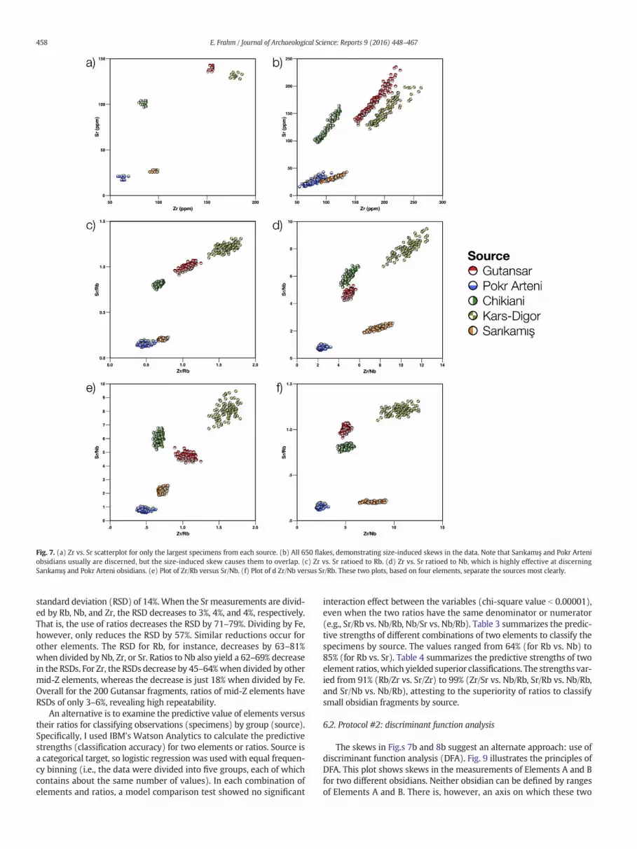
Fig. 7. (a) Zr vs. Sr scatterplot for only the largest specimens from each source. (b) All 650 flakes, demonstrating size-induced skews in the data. Note that Sarıkamış and Pokr Arteniobsidians usually are discerned, but the size-induced skew causes them to overlap. (c) Zr vs. Sr ratioed to Rb. (d) Zr vs. Sr ratioed to Nb, which is highly effective at discerningSarıkamış and Pokr Arteni obsidians. (e) Plot of Zr/Rb versus Sr/Nb. (f) Plot of d Zr/Nb versus Sr/Rb. These two plots, based on four elements, separate the sources most clearly.

458 E. Frahm / Journal of Archaeological Science: Reports 9 (2016) 448–467

standard deviation (RSD) of 14%. When the Sr measurements are divid-ed by Rb, Nb, and Zr, the RSD decreases to 3%, 4%, and 4%, respectively.That is, the use of ratios decreases the RSD by 71–79%. Dividing by Fe,however, only reduces the RSD by 57%. Similar reductions occur forother elements. The RSD for Rb, for instance, decreases by 63–81%when divided by Nb, Zr, or Sr. Ratios to Nb also yield a 62–69% decreasein the RSDs. For Zr, the RSDs decrease by 45–64%when divided by othermid-Z elements, whereas the decrease is just 18% when divided by Fe.Overall for the 200 Gutansar fragments, ratios of mid-Z elements haveRSDs of only 3–6%, revealing high repeatability.

An alternative is to examine the predictive value of elements versustheir ratios for classifying observations (specimens) by group (source).Specifically, I used IBM's Watson Analytics to calculate the predictivestrengths (classification accuracy) for two elements or ratios. Source isa categorical target, so logistic regression was used with equal frequen-cy binning (i.e., the data were divided into five groups, each of whichcontains about the same number of values). In each combination ofelements and ratios, a model comparison test showed no significant

interaction effect between the variables (chi-square value b 0.00001),even when the two ratios have the same denominator or numerator(e.g., Sr/Rb vs. Nb/Rb, Nb/Sr vs. Nb/Rb). Table 3 summarizes the predic-tive strengths of different combinations of two elements to classify thespecimens by source. The values ranged from 64% (for Rb vs. Nb) to85% (for Rb vs. Sr). Table 4 summarizes the predictive strengths of twoelement ratios,which yielded superior classifications. The strengths var-ied from 91% (Rb/Zr vs. Sr/Zr) to 99% (Zr/Sr vs. Nb/Rb, Sr/Rb vs. Nb/Rb,and Sr/Nb vs. Nb/Rb), attesting to the superiority of ratios to classifysmall obsidian fragments by source.

6.2. Protocol #2: discriminant function analysis

The skews in Fig.s 7b and 8b suggest an alternate approach: use ofdiscriminant function analysis (DFA). Fig. 9 illustrates the principles ofDFA. This plot shows skews in the measurements of Elements A and Bfor two different obsidians. Neither obsidian can be defined by rangesof Elements A and B. There is, however, an axis on which these two

Fig. 8. (a) Rb vs. Nb scatterplot for the largest specimens from each source. (b) All 650 flakes, showing the size-induced skew causes multiple overlaps: Pokr Arteni with Gutansar andChikiani with Kars-Digor. (c) Rb vs. Nb ratioed to Sr. (d) Rb vs. Nb ratioed to Zr.

459E. Frahm / Journal of Archaeological Science: Reports 9 (2016) 448–467

populations are discerned and the skew is minimized: line c–d. The axiscombines Elements A and B in a discriminant function (line e–f). Withadditional elements, DFA determines the best axes to discern popula-tions in higher dimensions. These derived functions can be also usedto classify additional observations (i.e., specimens, artifacts).

DFAwas applied to half of the fragments from each source (e.g., 100fragments from Gutansar), randomly selected, to derive functions thatmaximize separation of the sources and minimize skew. This analysiswas conducted using XLSTAT Pro (version 2013.2.01), and the samefour elements — Zr, Sr, Rb, and Nb — were included in the functions.One guideline is that the smallest group used to derive the functionsshould exceed the number of variables, ideally by a factor of three ormore (Williams and Titus, 1988). In this case, there were 50 fragmentsfor the Chikiani, Sarıkamış, and Kars-Digor sources (i.e., 12.5 moreobservations than variables). For each source and element, the valuesare largely normal (with mild positive skews ∼0.4–0.7) and no markedoutliers, satisfying DFA guidelines. The only case of moderate correla-tion among elements is that between Zr and Sr (0.86), which suggestscollinearity of variables is low, favorable to DFA. The resulting functionswere, in turn, used to classify the other half of the obsidian fragments.

Fig. 10a shows the 325 fragments used to derive discriminant func-tions as well as their resulting separation by source. The first function(F1) accounts for 54.8% of the between-group variance, and the second

Table 3Predictive strengths of two elements to sort the experimental flake assemblage byobsidian source.

Variable 1

Zr Sr Rb Nb

Variable 2 Zr – 80% 78% 72%Sr – 85% 82%Rb – 64%Nb –

one (F1) accounts for 28.2%, totaling 83.0% and attesting to a high dis-criminating power of this model. Prior and posterior classificationswere identical, exhibiting no erroneous classifications. A Wilks' lambdatest further attests that these obsidian sources are clearly differentiateddespite including irregular fragments as small as ∼2 mm in diameter.The nearer Wilks' lambda is to zero, the more the included variablescontribute to discrimination, and a chi-square statistic tests its signifi-cance. In this case, Wilks' lambda is b0.0001, and the p-value isb0.0001, showing that the functions well explain group membership.Fig. 10b illustrates how the other half of the fragments were classifiedusing these discriminant functions. The fragments fall in the sameregions of the scatterplot with even less spread and no marked outliers.

Thus, this approach also exhibits great promise for sourcing smallobsidian chips. A drawback, however, is that it necessitates considerableempirical work at first: onemust obtain fairly large obsidian specimens,reduce them into fragments of various sizes that reflect the assemblageof interest, analyze a sizable number of the fragments, and derivediscriminant functions using the resulting dataset. It also cannot beused with published element concentrations (unless there is a size ef-fect in those data). However, the power to minimize size-inducedskew and to include multiple elements in the calculation make thisa useful approach when a sufficient amount of source material isavailable.

7. Side effect of the protocols

Using elemental ratios to minimize systematic size-inducedmeasurement error will also minimize systematic compositional vari-ability (i.e., certain types of chemical zoning in an individual obsidianflow; e.g., correlated variation of elements in Borax Lake obsidian inCalifornia, Bowman et al., 1973). If present, such intra-source variationwill be reduced as well. This effect is best shown using a collection ofsynthetic specimens, the compositions of which were systemicallyadjusted over known ranges.

Table 4Predictive strengths of two element ratios to sort the experimental assemblage by obsidian source.

Variable 1

Zr/Rb Zr/Nb Zr/Sr Sr/Rb Sr/Nb Sr/Zr Rb/Nb Rb/Zr Rb/Sr Nb/Rb Nb/Zr Nb/Sr

Variable 2 Zr/Rb – 93% 92% 92% 98% 91% 95% – 92% 95% 93% 98%Zr/Nb – 95% 93% 94% 95% 95% 93% 93% 95% – 94%Zr/Sr – 96% 96% – 99% 92% 96% 99% 95% 96%Sr/Rb – 96% 95% 99% 92% – 99% 93% 96%Sr/Nb – 96% 99% 98% 96% 99% 94% –Sr/Zr – 99% 91% 95% 99% 95% 96%Rb/Nb – 95% 99% – 95% 99%Rb/Zr – 92% 95% 93% 98%Rb/Sr – 99% 93% 96%Nb/Rb – 95% 99%Nb/Zr – 94%Nb/Sr –

460 E. Frahm / Journal of Archaeological Science: Reports 9 (2016) 448–467

Composite specimens were made using (1) the sub-30-mm fractionof two levigated clays (Kilikoglou et al., 1998) and (2) quartz grains(∼99.5% SiO2). Quartz was added to the two clays in three volume frac-tions (5, 10, 20%) to predictably alter their compositions (i.e., elements'concentrations were “diluted” by the addition of nearly pure silica).Their mean particle sizes also varied (100, 250, 400, 750 μm).Accordingly, there were twelve composite specimens in addition toone specimen without quartz. After drying and firing, these thirteenspecimens were cut into rectangular prism bars ∼10 × 10 × 60 mmwith flat surfaces. Each specimen was measured fifteen times (each ina different spot). The XL3t GOLDD+ instrument was mounted in a

Fig. 9. Simplified example of two obsidian sources and their measured concentrations ofElements A and B. Neither one can be defined simply using ranges of Elements A and Bdue to overlaps. There is, though, an axis for which the two are differentiated: line c–d.The new axis combines Elements A and B into a discriminant function (line e–f).

Fig. 10. (a) Plot of the 325 obsidian fragments (circles) used to derive discriminant functionsirregular chips as small as ∼2 mm in diameter. (b) Plot with the other half of the fragmentregions of the plot with less spread and no marked outliers.

portable testing stand for these analyses. Themid-Z elements of interestweremeasured, as before, for 30 s with the “Main” filter in the “Mining”mode. These measurements were calibrated with a set of four certifiedstandards: CCRMP TILL-4, NRCCRM GBW07411, IAEA SOIL-7, and NCSDC73308.

Fig. 11 shows the data for these synthetic composites. All of themea-surements for Zr, Sr, Rb, and Nb are available in SOM Table B with a fullbreakdown by clay type and by particle size as well as volume fraction.The two populations in the data reflect the two clays in this test. Asexpected, Fig. 11a exhibits a “dilution” effect with additional quartzgrains. For example, Rb has a mean concentration of 132 ± 2 ppm inClay A without quartz. When the quartz reaches 20% by volume, themean Rb concentration is 108 ± 3 ppm in Clay A. This spread is not sosevere that the two clays overlap, but one can envision a situation inwhich that occurs. Fig. 11b reveals that, when the Rb and Sr datagraphed in Fig. 11a are divided by Nb, the clusters tighten. This occursbecause Nb has also been diluted systematically by quartz particles.Thus, compositional variability of the specimens is also minimized byratioing, emphasizing the presence of two different clays.

8. Archaeological example: Melos obsidians

This example is a follow-up to Frahm et al. (2014a), which showedthe effectiveness of pXRF for sourcing Aegean obsidians and notedthat the next phase of the work would include analyzing assemblagesfrom active excavations in local archaeological facilities. In particular,this example was chosen for two reasons: (1) the prismatic blades,

and their resulting separation by source. These sources are discerned despite includings (squares) classified using the derived discriminant functions and falling in the same

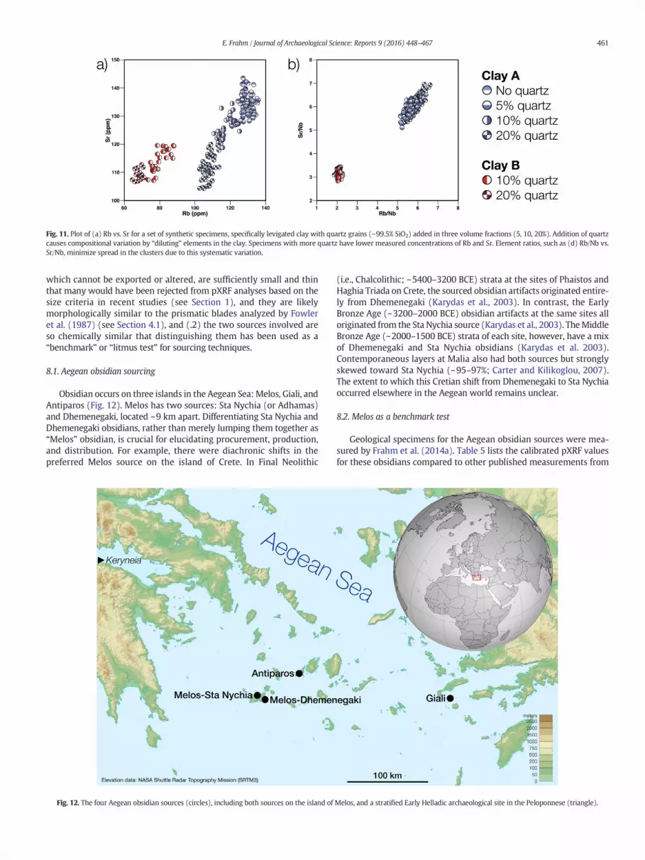
Fig. 11. Plot of (a) Rb vs. Sr for a set of synthetic specimens, specifically levigated clay with quartz grains (∼99.5% SiO2) added in three volume fractions (5, 10, 20%). Addition of quartzcauses compositional variation by “diluting” elements in the clay. Specimens with more quartz have lower measured concentrations of Rb and Sr. Element ratios, such as (d) Rb/Nb vs.Sr/Nb, minimize spread in the clusters due to this systematic variation.

461E. Frahm / Journal of Archaeological Science: Reports 9 (2016) 448–467

which cannot be exported or altered, are sufficiently small and thinthat many would have been rejected from pXRF analyses based on thesize criteria in recent studies (see Section 1), and they are likelymorphologically similar to the prismatic blades analyzed by Fowleret al. (1987) (see Section 4.1), and (.2) the two sources involved areso chemically similar that distinguishing them has been used as a“benchmark” or “litmus test” for sourcing techniques.

8.1. Aegean obsidian sourcing

Obsidian occurs on three islands in the Aegean Sea:Melos, Giali, andAntiparos (Fig. 12). Melos has two sources: Sta Nychia (or Adhamas)and Dhemenegaki, located ∼9 km apart. Differentiating Sta Nychia andDhemenegaki obsidians, rather than merely lumping them together as“Melos” obsidian, is crucial for elucidating procurement, production,and distribution. For example, there were diachronic shifts in thepreferred Melos source on the island of Crete. In Final Neolithic

Fig. 12. The four Aegean obsidian sources (circles), including both sources on the island of

(i.e., Chalcolithic; ∼5400–3200 BCE) strata at the sites of Phaistos andHaghia Triada on Crete, the sourced obsidian artifacts originated entire-ly from Dhemenegaki (Karydas et al., 2003). In contrast, the EarlyBronze Age (∼3200–2000 BCE) obsidian artifacts at the same sites alloriginated from the Sta Nychia source (Karydas et al., 2003). TheMiddleBronze Age (∼2000–1500 BCE) strata of each site, however, have a mixof Dhemenegaki and Sta Nychia obsidians (Karydas et al. 2003).Contemporaneous layers at Malia also had both sources but stronglyskewed toward Sta Nychia (∼95–97%; Carter and Kilikoglou, 2007).The extent to which this Cretian shift from Dhemenegaki to Sta Nychiaoccurred elsewhere in the Aegean world remains unclear.

8.2. Melos as a benchmark test

Geological specimens for the Aegean obsidian sources were mea-sured by Frahm et al. (2014a). Table 5 lists the calibrated pXRF valuesfor these obsidians compared to other published measurements from

Melos, and a stratified Early Helladic archaeological site in the Peloponnese (triangle).

Table5

Aeg

eanob

sidian

source

compo

sition

alda

tacompiledfrom

numerou

sstud

ies.

ThisStud

yGale19

81Sh

elford

etal.1

982

Fran

caviglia

1984

Kiliko

glou

etal.1

997

Gratuze

1999

Arias

etal.2

006

DeFran

cesco

etal.2

008

Liritzis20

08Ca

rter

&Co

ntreras20

12Milić20

14

pXRF

XRF

XRF

NAA

XRF

NAA

ICP-OES

ICP-MS

NAA

XRF

XRF

XRF

pXRF

Ove

rallMea

n

Dhe

men

egak

in=

16n=

6n=

18n=

3n=

63n=

6n=

4n=

3n=

5n=

40n=

11Rb

105±

211

1±

112

4±

411

3±

1011

4±

311

4±

797

±1

97±

310

9±

9Sr

127±

311

3±

111

5±

414

7±

212

8±

211

2±

511

0±

312

2±

13Zr

109±

314

0±

413

7±

211

1±

612

1±

113

0±

611

4±

512

3±

13StaNyc

hia

n=

28n=

8n=

74n=

27n=

60n=

5n=

5n=

4n=

9n=

30n=

8Rb

113±

311

9±

112

3±

611

8±

812

1±

312

0±

710

5±

710

8±

311

6±

7Sr

112±

399

±1

98±

211

7±

111

5±

398

±4

100±

410

6±

9Zr

99±

212

8±

412

4±

314

5±

1712

9±

3212

0±

410

7±

312

2±

15Antiparos

n=

12n=

7n=

11n=

5n=

5n=

40n=

1Rb

381±

839

6±

641

1±

240

3±

2737

6±

1736

738

9±

17Sr

7±

19±

12±

212

±2

108±

4Zr

127±

414

7±

617

0±

2014

6±

612

814

4±

18Giali

n=

16n=

26n=

6n=

4n=

1n=

4n=

2n=

20n=

5Rb

139±

314

9±

514

0±

613

413

7±

512

1±

213

7±

9Sr

69±

585

±6

6769

±1

72±

767

±5

63±

270

±7

Zr91

±5

110±

1078

±9

9110

3±

311

2±

696

±2

97±

12

462 E. Frahm / Journal of Archaeological Science: Reports 9 (2016) 448–467

a variety of analytical techniques. As shown in the table, Sta Nychia andDhemenegaki obsidians are similar in not only their appearance andknapping quality but also their chemical composition (due to theirshared volcanic origins). Their Rb values, for example, differ by ∼1–6%relative (depending on the precise dataset considered in Table 5).Their Zr values differ by ∼1–9%, whereas their Sr values differ by∼9–14%. In contrast, the other Aegean obsidian sources — Gialiand Antiparos — differ to much greater degrees: ∼90–100% for Rb,∼30–40% for Zr, and ∼140–190% for Sr.

Differentiating Sta Nychia andDhemenegaki obsidians has frequent-ly been used as a “benchmark” or “litmus test” to assess new techniquesfor sourcing obsidian. Some of themethodswere successful (e.g., NAA inAspinall et al., 1972; WDXRF in Shelford et al., 1982; rock magneticcharacterization in McDougall et al., 1983; ICP-OES in Kilikoglou et al.,1997; SEM-EDS in Acquafredda et al., 1999; Mössbauer spectroscopyin Stewart et al., 2003; PIXE in Eder et al., 2013). Of the successful tech-niques, many have since found widespread use in obsidian sourcing.Various other techniques were unable to differentiate Sta Nychia andDhemenegaki obsidians (e.g., fission-track dating in Durrani et al.,1971; strontium isotopes in Gale 1981; electrical conductivity inKotsakis 1982; inclusion mineralogy in Acquafredda and Paglionico2004; Raman spectroscopy in Arias et al., 2006; luminescence inPolymeris et al., 2010). The unsuccessful techniques have seen limited,if any, application in obsidian artifact sourcing. Hence, the Aegeanoften serves as a “proving ground.”

WDXRF and EDXRF techniques can usually distinguish specimens ofSta Nychia and Dhemenegaki obsidian (see Table 5), as can recent pXRFinstruments (Frahm et al., 2014a; Milić, 2014). The main goal of thisexample is demonstrating the success of the elemental ratio protocolin a setting well known as a challenge for sourcing methods.

8.3. Sourcing small Early Helladic blades

Here I demonstrate the use of elemental ratios with 200 obsidianartifacts excavated at a stratified Early Helladic site (EH I and II, 2650 to2000 BCE) in the Peloponnese along the Gulf of Corinth (the blacktriangle in Fig. 12; 38.212° N, 22.124° E). This settlement, previouslydescribed by Kolia (2012, 2013), was excavated from2009 to 2013 beforethe Olympia Motorway construction (I visited the site in 2012). Kolia(2013) proposes that the site, which spans N5 ha, was one of the earlyproto-urban centers that emerged in the Peloponnese at the time andthat it served as an administrative center for its surroundings during thethird millennium BCE. At this point in time, based on earlier resultsfrom Crete, a predominance of Sta Nychia obsidian would be anticipated.

The obsidian assemblage primarily consists of prismatic blades(including bladelets, segments, and other blade-based types). Thesetools were common throughout the Eastern Mediterranean and NearEast at this time (Frahm, 2014). The long and thin blades have trapezoi-dal or triangular cross-sections, hence the “prismatic” label. It iscommon for a 10-mm-wide prismatic blade to be ∼2 mm thick at itscenter, tapering to razor-thin edges on its sides. In terms of generalmorphology, these prismatic blades are likely similar to those sourcedby Fowler et al. (1987) using WDXRF and elemental ratios.

Fig. 13 shows 200 blades from the site. They primarily fall in a rangeof 6–12mmwide and 1–3mmmaximum thickness (at the apex of theirtriangular or trapezoidal cross-sections). Thus, many do not satisfy therequirements of an ideal XRF specimen and would have been excludedunder the criteria in recent studies (see Section 1). These blades were afocus specifically because they cannot be exported or subsampled.

These bladeswere also analyzedwith a Niton XL3t 950 GOLDD+ in-strument. Using the “Main” filter in “Mining”mode, themid-Z elementswere measured for 30 s, just as in Section 5.3. The setting (an archaeo-logical laboratory with other researchers around) compelled a differentphysical arrangement for conducting the pXRF analyses. Rather thanholding the instrument upright with an artifact atop it, the analyzerpointed downward in a custom stand, whereby it rested on an artifact

Fig. 13. Two hundred prismatic obsidian blades and bladelets sourced using pXRF. 198 of the blades (left) originated from the Sta Nychia obsidian source, whereas just two (right) insteadoriginated from the Dhemenegaki source.

463E. Frahm / Journal of Archaeological Science: Reports 9 (2016) 448–467

sitting on a low-density polyester (C10H8O4) substrate. In Section 6,non-ideal specimens yielded high measured concentrations due to en-hancement of a small, systematic error. Specifically, the softwareunderestimated small specimens' masses when they are surroundedby nothing but air. In this instance, however, with a polyester substrate,measured concentrations for non-ideal specimens were low due to thesoftware overestimating their masses. The measured element contentswere divided by too much mass due to the polyester substrate increas-ing X-ray scattering, producing low concentrations. Fig. 14 illustrateshow plots of elemental concentrations systematically skew lower thanthe values for the sources, causing artifacts from the two Melos sourcesto intermingle. Normalizing the measurements to a given element(Fig. 14d: Sr; e: Zr; f: Rb) reduces this skew and increases the separationbetween the sources. Therefore, the blades can bemore clearly attribut-ed to their sources. The 198 artifacts on the left side of Fig. 13 are madeof obsidian from Sta Nychia, whereas the two artifacts on the right sideare obsidian from Dhemenegaki. This is consistent with the anticipatedpredominance of Sta Nychia obsidian based on the available Bronze Agedatasets from Crete, suggesting that this pattern occurred over a largergeographic scale than the Greek islands.

9. Conclusions

This paper considers pragmatic solutions to the issues with sourcingsmall obsidian chips using EDXRF in general and pXRF in particular.

Earlier studies have examined these issues and offered various recom-mendations, including use of another technique (e.g., NAA, LA-ICP-MS) for small artifacts. To address this issue, this study used a largeexperimental assemblage: 650 flakes from five important obsidiansources in the Caucasus ecoregion (cf. 21 flakes from three sources inHughes, 2010; 78 flakes from one source in Nazaroff and Shackley,2009). Two data handling protocols enable reliable source identifica-tions down to microdebitage scales. The first protocol involves calculat-ing ratios between quantitative concentrations of “mid-Z” elements,which are well measured using pXRF and have similar characteristicX-ray energies, meaning that their signals are similarly influenced bysmall specimens. The second protocol uses multivariate analysis andexperimental assemblages to combine the element measurementsalong new axes that minimize size-induced skew. A side effect is thatthe approaches will “flatten” any systematic chemical variability withinan obsidian source, as demonstrated by experimental compositespecimens. Both approaches, however, can source small obsidianchips, down to scales of ∼1–2 mm (≤10 mg) and, thus, overcome theartifact size bias described by Eerkens et al. (2007).

As an example, 200 prismatic blades, excavated from an EarlyHelladic settlement in the Peloponnese, were analyzed and attributedto the two obsidian sources on the island of Melos. These blades weresufficiently small or thin that many would have been eliminated frompXRF analyses and sourcing according to recent criteria in the literature(e.g., Coffman and Rasic, 2015;Millhauser et al., 2015). Additionally, the

Fig. 14. Plots of (a) Rb vs. Zr, (b) Rb vs. Sr, and (c) Zr vs. Sr for the Aegean sources and obsidian blades. These artifact data skew lower than the values for the sources, causing artifacts fromthe twoMelos sources to intermingle.Normalizing themeasurements to a given element— (d) Sr, (e) Zr, and (f) Rb— reduces the overlap and enhances separation between the Sta Nychiaand Dhemenegaki sources.

464 E. Frahm / Journal of Archaeological Science: Reports 9 (2016) 448–467

two Melos obsidian sources are similar in composition, so distinguishingthem has been used as a means to assess obsidian sourcing techniques.Using elemental ratios, 198 artifacts were matched to the Sta Nychiasource, while two were matched to the Dhemenegaki source. This resultis consistent with the predominance of Sta Nychia obsidian on Creteduring the Bronze Age, suggesting that the same pattern in sourceexploitation occurred beyond the Greek islands.

Supplementary data to this article can be found online at http://dx.doi.org/10.1016/j.jasrep.2016.08.032.

Acknowledgments

Many friends and colleagues made this study possible. I thank PavelAvetisyan, Director of the Institute for Archaeology and Ethnography,Armenia, for his continued support. I direct the Obsidian Resources andLandscapes of Palaeolithic Armenia project jointly with Boris Gasparyan,Institute of Archaeology and Ethnography, andDaniel S. Adler, Universityof Connecticut. My fieldwork was facilitated by Khachatur Meliksetianand Sergei Karapetian, Institute of Geological Sciences, Armenia,and Suren Kesejyan, Institute of Archaeology and Ethnography. Other

obsidian specimens were collected by George “Rip” Rapp, University ofMinnesota–Duluth, and the late Tuncay Ercan, General Directorate ofMineral Research and Exploration, Republic of Turkey. I am grateful tothe staff of the 6th Ephorate of Prehistoric and Classical Antiquities formaking arrangements forme to analyze the obsidian blades. The excava-tionwas conducted by the 6th Ephorate, andmy resultswere included ina 2012 report to the excavators and ephorate director. Funding for me toconduct analyses at the ephorate was provided by the Marie CurieNARNIA project (Grant 265010). Artifact photos are included withoutfee thanks to the exemption granted to scientific studies and publications.The synthetic specimens were made by Vassilis Kilikoglou, NationalCentre for Scientific Research “Demokritos.” Liev Frahm assisted withtheir measurement. One of the Niton instruments in this study is ownedby the University of Sheffield's Archaeology Department, and the otherpXRF is part of the research infrastructure of the Institute for RockMagne-tism, Department of Earth Sciences, University of Minnesota. NAA andEDXRF data were provided byMichael Glascock, Archaeometry Laborato-ry, MURR. EMPA analyses were conducted in the Electron MicroprobeLaboratory, the University of Minnesota. Three anonymous reviewers'comments improved the clarity of the final manuscript.

465E. Frahm / Journal of Archaeological Science: Reports 9 (2016) 448–467

Refereneces

Abbès, F., Bellot-Gurlet, L., Cauvin, M.-C., Delerue, S., Dubernet, S., Poupeau, G., Stordeur,D., 2003. Provenance of the Jerf el Ahmar (Middle Euphrates Valley, Syria) obsidians.J. Non-Cryst. Solids 323 (1-3), 162–166.

Acquafredda, P., Paglionico, A., 2004. SEM–EDS microanalysis of microphenocrysts ofMediterranean obsidians: a preliminary approach to source discrimination. Eur.J. Mineral. 16, 419–429.

Acquafredda, P., Andriani, T., Lorenzoni, S., Zanettin, E., 1999. Chemical characterization ofobsidians from different Mediterranean sources by non-destructive SEM-EDSanalytical method. J. Archaeol. Sci. 26 (3), 315–325.

Adler, D.S., Conard, N.J., 2005. Tracking Hominins during the last interglacial complex inthe Rhineland. In: Gamble, C., Porr, M. (Eds.), In The Individual Hominid in Context:Archaeological Investigations of Lower and Middle Palaeolithic Landscapes, Locales,and Artefacts. Routledge Press, London, pp. 133–153.

Adler, D.S., Wilkinson, K.N., Blockley, S., Mark, D., Pinhasi, R., Schmidt-Magee, B.,Nahapetyan, S., Mallol, C., Berna, F., Glauberman, P., Raczynski-Henk, Y., Wales, N.,Frahm, E., Jöris, O., MacLeod, A., Smith, V., Cullen, V., Gasparyan, B., 2014. EarlyLevallois technology and the transition from the Lower to Middle Palaeolithic in theSouthern Caucasus. Science 345 (6204), 1609–1613.

Alperson-Afil, N., 2008. Continual fire-making by Hominins at Gesher Benot Ya‘aqov,Israel. Quat. Sci. Rev. 27, 1733–1739.

Arias, A., Oddone, M., Bigazzi, G., Di Muro, A., Principe, C., Norelli, P., 2006. New data forthe characterization of Milos obsidians. J. Radioanal. Nucl. Chem. 268, 371–386.

Aspinall, A., Feather, S., Renfrew, C., 1972. Neutron activation analysis of Aegeanobsidians. Nature 237, 333–334.

Badalyan, R., Chataigner, C., Kohl, P., 2004. Trans-Caucasian obsidian: the exploitation ofthe sources and their distribution. In: Sagona, A. (Ed.), A View from the Highlands:Archaeological Studies in Honour of Charles Burney. Peeters, Lueven, pp. 437–465.

Bar-Oz, G., Weissbrod, L., Gasparian, B., Nahapetyan, S., Wilkinson, K.N., Pinhasi, R., 2012.Taphonomy and zooarchaeology of a high-altitude Upper Pleistocene faunalsequence from Hovk-1 Cave, Armenia. J. Archaeol. Sci. 39, 2452–2463.

Barton, R.N.E., Jennings, R. P. 2012. The lithic assemblages of Gorham's Cave. In Neander-thals in context. A Report of the 1995-1998 Excavations at Gorham's and VanguardCaves, Gibraltar, edited by R.N.E. Barton, C.B. Stringer, and J.C. Finlayson, pp. 151-187. Oxford University School of Archaeology: Monograph 75.

Baumler, M.F., Davis, L.B., 2004. The role of small-sized debitage in aggregate lithicanalysis. In: Larson, M.L., Hall, C.T. (Eds.), Aggregate Analysis in Chipped Stone.University of Utah Press, Salt Lake City, Utah, pp. 45–64.

Blackman, M.J., Badalian, R., Kikodze, Z., Kohl, P., 1998. Chemical characterization ofcaucasian obsidian geological sources. In: Cauvin, M.-C., Gourgaud, A., Gratuze, B.,Arnaud, N., Poupeau, G., Poidevin, J.L., Chataigner, C. (Eds.), L'obsidienne au Procheet Moyen-Orient: Du Volcan à l'Outil. BAR International Series, pp. 205–231.

Bowman, H., Asaro, F., Pearlman, I., 1973. Composition Variations in Obsidian Sources andthe Archaeological Implications. Archaeometry 15 (1), 123–127.

Brumm, A., Boivin, N., Korisettar, R., Koshy, J., Whittaker, P., 2007. Stone axe technology inNeolithic South India: new evidence from the Sanganakallu-Kupgal Region,Mideastern Karnataka. Asian Perspect. 46, 65–95.

Cann, J.R., Renfrew, C., 1964. The characterization of obsidian and its application to theMediterranean Region. Proceedings of the Prehistoric Society 30, 111–133.

Carter, T., Contreras, D., 2012. The character and use of the Soros Hill obsidian source,Antiparos (Greece). C.R. Palevol 11, 595–602.

Carter, T., Kilikoglou, V., 2007. From reactor to royalty? Aegean and Anatolian obsidiansfrom Quartier Mu, Malia (Crete). J. Mediterr. Archaeol. 20, 1–29.

Carter, T., Poupeau, G., Bressy, C., Pearce, N., 2006. A new programme of obsidiancharacterization at Çatalhöyük, Turkey. J. Archaeol. Sci. 33 (7), 893–909.

Chataigner, C., Gratuze, B., 2014a. New data on the exploitation of obsidian in the south-ern Caucasus (Armenia, Georgia) and eastern Turkey, part 1: source characterization.Archaeometry 56, 25–47.

Chataigner, C., Gratuze, B., 2014b. New data on the exploitation of obsidian in the south-ern Caucasus (Armenia, Georgia) and eastern Turkey, part 2: obsidian procurementfrom the Upper Palaeolithic to the Late Bronze Age. Archaeometry 56, 48–69.

Coffman, S., Rasic, J.T., 2015. Rhyolite characterization and distribution in central Alaska.J. Archaeol. Sci. 57, 142–157.

Conard, N.J., Adler, D.S., 1997. Lithic reduction and hominid behavior in the MiddlePaleolithic of the Rhineland. J. Anthropol. Res. 53 (2), 147–175.

Conard, N.J., Kandel, A.W., 2006. The economics and settlement dynamics of the laterHolocene inhabitants of near coastal environments in the West Coast National Park(South Africa). In: Wotzka, H.-P. (Ed.), Grundlegungen: Beiträge zur europäischenund afrikanischen Archäologie für Manfred K. H. Eggert. Francke, Tübingen,pp. 329–355.

Craig, N., Speakman, R.J., Popelka-Filcoff, R., Glascock, M.D., Robertson, J., Shackley, M.S.,Aldenderfer, M., 2007. Comparison of XRF and PXRF for analysis of archaeologicalobsidian from southern Perú. J. Archaeol. Sci. 34, 2012–2024.

Davis, M.K., Jackson, T.L., Shackley, M.S., Teague, T., Hampel, J.H., 1998. Factors affectingthe energy-dispersive X-ray fluorescence (EDXRF) analysis of archaeologicalobsidian. In: Shackley, M.S. (Ed.), Archaeological Obsidian Studies: Method andTheory. Plenum, New York, pp. 159–180.

Davis, M.K., Jackson, T.L., Shackley, M.S., Teague, T., Hampel, J.H., 2011. Factors affectingthe energy-dispersive X-ray fluorescence (EDXRF) analysis of archaeologicalobsidian. In: Shackley, M.S. (Ed.), X-ray Fluorescence Spectrometry (XRF) inGeoarchaeology. Springer, pp. 45–63.

De Francesco, A.M., Crisci, G.M., Bocci, M., 2008. Non-destructive analytic methodusing XRF for determination of provenance of archaeological obsidians from theMediterranean Area: a comparison with traditional XRF methods. Archaeometry 50(2), 337–350.

Dietl, H., Kandel, A.W., Conard, N.J., 2005. Middle Stone Age settlement and land use at theopen-air sites of Geelbek and Anyskop, South Africa. Journal of African Archaeology 3(2), 233–244.

Dunnell, R.C., Stein, J.K., 1989. Theoretical issues in the interpretation of microartifacts.Geoarchaeology 4 (1), 31–42.

Durrani, S., Khan, M., Renfrew, C., 1971. Obsidian source identification by fission trackanalysis. Nature 233, 242–252.

Eder, F.M., Neelmeijer, C., Pearce, N.J.G., Bichler, M., Sterba, J.H., Ntaflos, T., Merchel, S.,2013. Volcanic glass under fire – a comparison of three complementary analyticalmethods. X-Ray Spectrom. 42, 412–422.

Eerkens, J., King, J., Glascock, M.D., 2002. Artifact size and chemical sourcing: Studyingthe potential biases of selecting large artifacts for analysis. SCA Newsletter 36 (3),25–29.

Eerkens, J., Ferguson, J., Glascock, M.D., Skinner, C., Waechter, S., 2007. Reduction strate-gies and geochemical characterization of lithic assemblages: a comparison of threecase studies from western North America. Am. Antiq. 72, 585–597.

Egeland, C.P., Gasparian, B., Arakelyan, D., Nicholson, C.M., Petrosyan, A., Ghukasyan, R.,Byerly, R., 2014. Reconnaissance survey for Palaeolithic sites in the Debed RiverValley, northern Armenia. Journal of Field Archaeology 39 (4), 370–386.

Escola, P.S., Hocsman, S., Babot, M.P., 2016. Moving Obsidian: The Case of Antofagasta dela Sierra basin (Southern Argentinean Puna) During the Late Middle and LateHolocene. Quaternary International (in press, online early view).

Ferguson, J.R., 2012. Chapter 12: X-ray fluorescence of obsidian: approaches to calibrationand the analysis of small samples. In: Shugar, A.N., Mass, J.L. (Eds.), Handheld XRF forArt and Archaeology. Leuven University Press, Leuven, pp. 401–422.

Fladmark, K.R., 1982. Microdebitage analysis: Initial considerations. J. Archaeol. Sci. 9 (2),205–220.

Fornaseri, M., Malpieri, L., Palmieri, A.M., Taddeucci, A., 1975. Analyses of obsidians fromthe Late Chalcolithic levels of Arslantepe (Malatya). Paléorient 3 (1), 231–246.

Forster, N., Grave, P., 2012. Non-destructive PXRF analysis of museum-curated obsidianfrom the Near East. J. Archaeol. Sci. 39, 728–736.

Forster, N., Grave, P., Vickery, N., Kealhofer, L., 2011. Non-destructive analysis using PXRF:methodology and application to archaeological ceramics. X-Ray Spectrom. 40,389–398.

Fowler, W.R., Kelley, J.H., Asaro, F., Michel, H.V., Stross, F.H., 1987. The chipped stoneindustry of Cihuatan and Santa Maria, El Salvador, and sources of obsidian fromCihuatan. Am. Antiq. 52 (1), 151–160.

Frahm, E., 2010. The Bronze-age obsidian industry at Tell Mozan (ancient Urkesh), Syria.Ph.D. dissertation. Department of Anthropology, University of Minnesota. Universityof Minnesota’s Digital Conservancy: http://purl.umn.edu/99753.

Frahm, E., 2012. Non-destructive sourcing of Bronze-Age near eastern obsidian artefacts:redeveloping and reassessing electron microprobe analysis for obsidian sourcing.Archaeometry 54 (4), 623–642.

Frahm, E., 2013. Validity of “off-the-shelf” handheld portable XRF for sourcing NearEastern obsidian chip debris. J. Archaeol. Sci. 40, 1080–1092.

Frahm, E., 2014. Characterizing obsidian sources with portable XRF: accuracy, reproduc-ibility, and field relationships in a case study from Armenia. J. Archaeol. Sci. 49,105–125.

Frahm, E., Feinberg, J.M., 2013. Environment and collapse: Eastern Anatolian Obsidians atUrkesh (Tell Mozan, Syria) and the third-millennium Mesopotamian urban crisis.J. Archaeol. Sci. 40 (4), 1866–1878.

Frahm, E., Feinberg, J.M., 2015. Reassessing obsidian field relationships at Glass Buttes,Oregon. J. Archaeol. Sci. 665 (Reports 2), 654.

Frahm, E., Doonan, R.C.P., Kilikoglou, V., 2014a. Handheld portable X-ray fluorescence ofAegean obsidians. Archaeometry 56, 228–260.

Frahm, E., Schmidt, B., Gasparyan, B., Yeritsyan, B., Karapetian, S., Meliksetian, K., Adler,D.S., 2014b. Ten seconds in the field: rapid Armenian obsidian sourcing with portableXRF to inform excavations and surveys. J. Archaeol. Sci. 41, 333–348.

Francaviglia, V., 1984. Characterization of Mediterranean obsidian sources by classicalpetrochemical methods. Preistoria Alpina 20, 311–332.

Freund, K.P., 2014. Obsidian consumption in Chalcolithic Sardinia: a view from Bingia 'eMonti. J. Archaeol. Sci. 41, 242–250.

Gale, N., 1981. Mediterranean obsidian source characterization by strontium isotopeanalysis. Archaeometry 23, 41–51.

Galipaud, J.-C., Reepmeyer, C., Torrence, R., Kelloway, S., White, P., 2014. Long-distanceconnections in Vanuatu: new obsidian characterisations for the Makue site, AoreIsland. Archaeol. Ocean. 49 (2), 110–116.

Ghukasyan, R., Colonge, D., Nahapetyan, S., Ollivier, V., Gasparyan, B., Monchot, H.,Chataigner, C., 2011. Kalavan-2 (North of Lake Sevan, Armenia): a new LateMiddle Paleolithic site in the lesser Caucasus. Archaeology Ethnology & Anthropologyof Eurasia 38 (4), 39–51.

Glascock, M.D., 2011. Chapter 8: comparison and contrast between XRF and NAA:used for characterization of obsidian sources in central Mexico. In: Shackley, M.S.(Ed.), X-Ray Fluorescence Spectrometry (XRF) in Geoarchaeology. Springer,pp. 161–192.

Glascock, M.D., Ferguson, J.R., 2016. Frequently Asked Questions. Archaeometry Laborato-ry at the University of Missouri Research Reactor websitehttp://archaeometry.missouri.edu/faq.html (Accessed June 2016).

Golitko, M., 2011. Provenience investigations of ceramic and obsidian samples using laserablation inductively coupled plasma mass spectrometry and portable X-Rayfluorescence. Fieldiana Anthropology 42, 251–287.

Goodale, N., Bailey, D., Jones, G., Prescott, C., Scholz, E., Stagliano, N., Lewis, C., 2012. pXRF:a study of inter-instrument performance. J. Archaeol. Sci. 39, 875–883.

Gratuze, B., 1999. Obsidian characterization by laser ablation ICP–MS and its applicationto prehistoric trade in the Mediterranean and the Near East: sources and distributionof obsidian within the Aegean and Anatolia. J. Archaeol. Sci. 26, 869–881.

466 E. Frahm / Journal of Archaeological Science: Reports 9 (2016) 448–467

Hall, C.T., 2004. Evaluating prehistoric hunter-gatherer mobility, land use, and technolog-ical organization strategies. In: Larson, M.L., Hall, C.T. (Eds.), Aggregate Analysis inChipped Stone. University of Utah Press, Salt Lake City, Utah, pp. 139–155.

Hassan, F.A., 1978. Sediments in archaeology: methods and implications forpaleoenvironmental and cultural analysis. Journal of Field Archaeology 5, 197–213.

Hayden, B., Cannon, A., 1983. Where the garbage goes. J. Anthropol. Archaeol. 2, 117–163.Heginbotham, A., Bezur, A., Bouchard, M., Davis, J.M., Eremin, K., Frantz, J.H., Glinsman, L.,

Hayek, L.-A., Hook, D., Kantarelou, V., Germanos Karydas, A., Lee, L., Mass, J., Matsen,C., McCarthy, B., McGath, M., Shugar, A., Sirois, J., Smith, D., Speakman, R.J., 2010. Anevaluation of inter-laboratory reproducibility for quantitative XRF of historic copperalloys. In: Mardikian, P., et al. (Eds.), Metal 2010. Proceedings of the InternationalConference on Metal Conservation, Charleston, South Carolina, USA, October 11–15,2010. Clemson University Press, pp. 244–255.

Hughes, R.E., 2007. The geologic sources for obsidian artifacts from Minnesota archaeo-logical sites. The Minnesota Archaeologist 6, 53–68.

Hughes, R.E., 2010. Determining the geologic provenance of tiny obsidian flakes inarchaeology using nondestructive EDXRF. Am. Lab. 42, 27–31.

Hull, K.L., 1987. Identification of cultural site formation processes through microdebitageanalysis. Am. Antiq. 52, 772–783.

Jack, R.N., Heizer, R.F., 1968. “Finger-printing” of some Mesoamerican obsidian artifacts.Contributions of the University of California Archaeological Research Facility. 5,pp. 81–100.

Karapetian, S.G., Bashian Jr., R., Mnatsakanian, A.K., 2001. Late collision rhyolitic volcanismin the north-eastern part of the Armenian Highland. J. Volcanol. Geotherm. Res. 112,189–220.

Karydas, A., La Rosa, V., Militello, P., Pappalardo, G., Pappalardo, L., Rizzo, F., Romano, F.P.,2003. Provenance of obsidian artefacts from different archaeological layers ofPhaistos and Haghia Triada. Creta Antica 4, 287–300.

Keller, J., Seifried, C., 1990. The present status of obsidian source identification in Anatoliaand the Near East. PACT 25, 57–87.

Kellett, L.C., Golitko, M., Bauer, B.S., 2013. A provenance study of archaeological obsidianfrom the Andahuaylas region of southern Peru. J. Archaeol. Sci. 40, 1890–1902.

Khalidi, L., Gratuze, B., Boucetta, S., 2009. Provenance of obsidian excavated from LateChalcolithic levels at the sites of Tell Hamoukar and Tell Brak, Syria. Archaeometry51 (6), 879–893.

Kilikoglou, V., Bassiakos, Y., Doonan, R., Stratis, J., 1997. NAA and ICP analysis of obsidianfrom Central Europe and the Aegean: source characterisation and provenancedetermination. J. Radioanal. Nucl. Chem. 216, 87–93.

Kilikoglou, V., Vekinis, G., Maniatis, Y., Day, P.M., 1998.Mechanical performance of quartz-tempered ceramics: part I, strength and toughness. Archaeometry 40, 261–279.

Kolia, E., 2012. Aigialeia. In: Vlachopoulos, A. (Ed.), Αρχαιολογία Πελοπόννησος(Archaeology Peloponnese). Melissa Publications, Athens, pp. 324–331.

Kolia, E., 2013. Archaeological Research in Eastern Achaea Within the Framework ofLarge-Scale Technical Works. Αρχαιολογία Online. Online at http://www.archaeology.wiki/blog/2013/12/16/archaeological-research-in-eastern-achaea(accessed September 2015).

Kotsakis, G., 1982. On the electrical conductivity of the obsidian from Milos (Greece) in thetemperature range 250 °C–600 °C. Neues Jahrb. Mineral. Monatshefte 10, 471–480.

Larson, M.L., Kornfeld, M., 1997. Chipped stone nodules: theory, method, and examples.Lithic Technology 22, 4–18.

Le Bourdonnec, F.-X., Nomade, S., Poupeau, G., Hervé, G., Tushabramishvili, N., Moncel, M.-H., Pleurdeau, D., Agapishvili, T., Voinchet, P., Mgeladze, A., Lordkipanidze, D., 2012.Multiple origins of Bondi Cave and Ortvale Klde (NW Georgia) obsidians andhuman mobility in Transcaucasia during the Middle and Upper Palaeolithic.J. Archaeol. Sci. 39, 1317–1330.

Liritzis, I., 2008. Assessment of Aegean obsidian sources by a portable ED-XRF analyser:grouping, provenance and accuracy. In: Facorellis, Y., Zacharias, N., Polikreti, K.(Eds.), Proceedings of the 4th Symposium of the Hellenic Society for Archaeometry,BAR International Series 1746. Oxford.

Liritzis, I., Zacharias, N., 2011. Chapter 6: portable XRF of archaeological artifacts: currentresearch, potentials and limitations. In: Shackley, M.S. (Ed.), X-ray FluorescenceSpectrometry (XRF) in Geoarchaeology. Springer, pp. 109–142.

Lundblad, S.P., Mills, P.R., Hon, K., 2008. Analysing archaeological basalt using non-destructive energy-dispersive X-Ray fluorescence (EDXRF): effects of post-depositional chemical weathering and sample size on analytical precision.Archaeometry 50, 1–11.

Martínez-Moreno, Mora, R., de la Torre, I., 2010. The Middle-to-Upper Palaeolithic transi-tion in Cova Gran (Catalunya, Spain) and the extinction of Neanderthals in the IberianPeninsula. J. Hum. Evol. 58, 211–226.

McDougall, J.M., Tarling, D.H., Warren, S.E., 1983. The magnetic sourcing of obsidiansamples from Mediterranean and Near Eastern Sources. J. Archaeol. Sci. 10, 441–452.

Mercader, J., Martı ́, R., González, I.J., Sánchez, A., Garcı ́a, P., 2003. Archaeological siteformation in rain forests: insights from the Ituri Rock Shelters, Congo. J. Archaeol.Sci. 30, 45–65.

Merrick, H., Brown, F., 1984. Rapid chemical characterization of obsidian artifacts byelectron microprobe analysis. Archaeometry 26 (2), 230–236.

Metcalfe, D., Heath, K.M., 1990. Microrefuse and site structure: the hearths and floors ofthe Heartbreak Hotel. Am. Antiq. 55, 781–796.

Milić, M., 2014. PXRF characterisation of obsidian from central Anatolia, the Aegean andcentral Europe. J. Archaeol. Sci. 41, 285–296.

Millhauser, J., Rodríguez-Alegría, E., Glascock, M.D., 2011. Testing the accuracy of portableX-ray fluorescence to study Aztec and Colonial obsidian supply at Xaltocan, Mexico.J. Archaeol. Sci. 38, 3141–3152.

Millhauser, J.K., Fargher, L.F., Espinoza, V.Y.H., Blanton, R.E., 2015. The geopolitics ofobsidian supply in Postclassic Tlaxcallan: a portable X-ray fluorescence study.J. Archaeol. Sci. 58, 133–146.

Montoya, C., Balasescu, A., Joannin, S., Ollivier, V., Liagre, J., Nahapetyan, S., Ghukasyan, R.,Colonge, D., Gasparyan, B., Chataigner, C., 2013. The Upper Palaeolithic site of Kalavan1 (Armenia): an Epigravettian settlement in the Lesser Caucasus. J. Hum. Evol. 65,621–640.

Mulrooney, M.A., McAlister, A., Stevenson, C.M., Morrison, A.E., Gendreau, L., 2014. Sourc-ing Rapa Nui mata‘a from the collections of Bishop Museum using non-destructivepXRF. Journal of the Polynesian Society 123 (3), 301–338.

Nadel, D., 2001. Indoor/outdoor flint knapping and minute debitage remains: the evi-dence from the Ohalo II submerged camp (19.5 ky, Jordan Valley). Lithic Technology26 (2), 118–137.

Nazaroff, A., Shackley, M.S., 2009. Testing the size dimension limitation of portable XRFinstrumentation for obsidian provenance. Session: Obsidian from Magma to Artifact:Geological and Archaeological Perspectives. Geological Society of America AnnualMeeting, Portland, Oregon, 18–21 October 2009.

Nelson, E., 1975. Uses of X-ray fluorescence analysis in archaeology. Syesis 8, 91–95.Neri, L.A.M., Pawlik, A.F., Reepmeyer, C., Mijares, A.S.B., Paz, V.J., 2015. Mobility of early

islanders in the Philippines during the Terminal Pleistocene/Early Holoceneboundary: pXRF-analysis of obsidian artefacts. J. Archaeol. Sci. 61, 149–157.

Parks, G.A., Tieh, T.T., 1966. Identifying the geographical source of artefact obsidian.Nature 211 (5046), 289–290.

Peacock, E., Fant, D.W., 2002. Biomantle formation and artifact translocation in uplandsandy soils: an example from the Holly Springs National Forest, north-central Missis-sippi, U.S.A. Geoarchaeology: An International Journal 17, 91–114.

Pinhasi, R., Gasparian, B., Wilkinson, K., Schreve, D., Branch, N., Nahapetyan, S., 2006. Thearchaeology of Hovk, north-east Armenia: a preliminary report. Antiquity 80 (308),Project Gallery.

Pinhasi, R., Gasparian, B., Wilkinson, K., Bailey, R., Bar-Oz, G., Bruch, A., Chataignerg, C.,Hoffmann, D., Hovsepyan, R., Nahapetyan, S., Pike, A.W.G., Schreve, D., Stephens, M.,2008. Hovk 1 and the Middle and Upper Paleolithic of Armenia: a preliminary frame-work. J. Hum. Evol. 55, 803–816.

Pinhasi, R., Gasparian, B., Nahapetyan, S., Bar-Oz, G., Weissbrod, L., Bruch, A.A., Hovsepyan,R., Wilkinson, K., 2011. Middle Palaeolithic human occupation of the high altituderegion of Hovk-1, Armenia. Quat. Sci. Rev. 30, 3846–3857.

Poidevin, J.-L., 1998. Les Gisements d'Obsidienne de Turquie et de Transcaucasie:Géologie, Géochimie et Chronométrie. In: Cauvin, M.-C., Gourgaud, A., Gratauze, B.,Arnaud, N., Poupeau, G., Poidevin, J.L., Chataigner, C. (Eds.), L'obsidienne au Procheet Moyen-Orient: Du vVolcan à l'Outil. British Archaeological Reports. Maison del'Orient Méditerranéen, Archaeopress, Oxford, pp. 105–167.

Polymeris, G.S., Gogou, D., Afouxenidis, D., Rapti, S., Tsirliganis, N.C., Kitis, G., 2010. Prelim-inary TL and OSL investigations of obsidian samples. Mediterranean Archaeology andArchaeometry 10 (4), 83–91.

Potts, P.J., Williams-Thorpe, O., Webb, P.C., 1997. The bulk analysis of silicate rocks byportable X-ray fluorescence: effect of sample mineralogy in relation to the size ofthe excited volume. Geostand. Newslett. 21, 29–41.

Poupeau, G., Le Bourdonnec, F.-X., Carter, T., Delerue, S., Barrat, J.-A., Shackley, M.S.,Dubernet, S., Moretto, P., Calligaro, T., Milić, M., Kobayashi, K., 2010. The useof SEM-EDS, PIXE, and EDXRF for obsidian provenance studies in the Near East: acase study from Neolithic C ̦atalhöyük (central Anatolia). J. Archaeol. Sci. 37,2705–2720.

Renfrew, C., Cann, J., Dixon, J., 1965. Obsidian in the Aegean. Annual of the British Schoolat Athens 60, 225–247.

Renfrew, C., Dixon, J., Cann, J., 1966. Obsidian and early cultural contact in the Near East.Proc. Prehist. Soc 2, 30–72.

Shackley, M.S., 1988. Sources of archaeological obsidian in the southwest: an archaeolog-ical, petrological, and geochemical study. Am. Antiq. 53 (4), 752–772.

Shackley, M.S., 2011. An introduction to X-Ray fluorescence (XRF) analysis in archaeology.In: Shackley, M.S. (Ed.), X-Ray Fluorescence Spectrometry (XRF) in Geoarchaeology.Springer, pp. 7–44.

Shackley, M.S., 2012a. Portable X-ray fluorescence spectrometry (pXRF): the good, thebad, and the ugly (online essay). Archaeology Southwest Magazine 26 (Spring issue).

Shackley, M.S., 2012b. Thoughts on natural and manufactured glass studies in a 21st-century archaeology. In: Liritzis, I., Stevenson, C.M. (Eds.), Obsidian and AncientManufactured Glasses. University of New Mexico Press, pp. 202–210.

Shea, J.J., 2011. Homo sapiens is as Homo sapiens was. Curr. Anthropol. 52 (1), 1–35.Shelford, P., Hodson, F., Cosgrove, M.E.,Warren, S.E., Renfrew, C., 1982. The obsidian trade.

In: Renfrew, C., Wagstaff, J.M. (Eds.), An Island Polity: The Archaeology of Exploitationin Melos. Cambridge University Press, pp. 182–221.

Sheppard, P., Irwin, G., Lin, S., McCaffrey, C., 2011. Characterization of New Zealandobsidian using PXRF. J. Archaeol. Sci. 38, 45–56.

Sherwood, S.C., 2001. Microartifacts. In: Goldberg, P., Holliday, V.T., Ferring, C.R. (Eds.),Earth Sciences and Archaeology. Springer, pp. 327–351.

Shott, M.J., 1994. Size and form in the analysis of flake debris: review and recentapproaches. Journal of Archaeological Method and Theory 1, 69–110.

Stein, J.K., Teltser, P.A., 1989. Size distributions of artifact classes: combining macro-andmicro-fractions. Geoarchaeology 4, 1–30.

Stewart, S., Cernicchiaro, G., Scorzelli, R., Poupeau, G., Acquafredda, P., De Francesco, A.,2003. Magnetic properties and 57Fe Mössbauer spectroscopy of mediterranean pre-historic obsidians for provenance studies. J. Non-Cryst. Solids 323 (1–3), 188–192.

Summerhayes, G., Bird, J.R., Fullagar, R., Gosden, C., Specht, J., Torrence, R., 1998. Applica-tion of PIXE-PIGME to archaeological analysis of changing patterns of obsidian use inWest New Britain, Papua New Guinea. In: Shackley, M.S. (Ed.), ArchaeologicalObsidian Studies: Method and Theory. Plenum Press, New York, pp. 129–158.

Torrence, R., White, P., Kelloway, S., 2012. Expanding the range of pXRF to ethnographiccollections. International Association for Obsidian Studies Bulletin 46, 9–15.

Turq, A., Roebroeks, W., Bourguignon, L., Faivre, J.-P., 2013. The fragmented character ofMiddle Palaeolithic stone tool technology. J. Hum. Evol. 65, 641–655.

467E. Frahm / Journal of Archaeological Science: Reports 9 (2016) 448–467

Tykot, R.H., 1995. Prehistoric Trade in the Western Mediterranean: The Sources andDistribution of Sardinian Obsidian. PhD Dissertation. Harvard University.

Vaquero, M., Chacón, M.G., Cuartero, F., García-Antón, M.D., Gómez de Soler, B., Martínez,K., 2012. Chapter 7: the lithic assemblage of level J. In: Roura, E.C.i. (Ed.), HighResolution Archaeology and Neanderthal Behavior: Time and Space 189 in Level Jof Abric Romaní (Capellades, Spain). Springer.

Whittaker, J.C., Kamp, K.A., Ford, A., Guerra, R., Brands, P., Guerra, J., Mclean, K., Woods, A.,Badillo, M., Thornton, J., Eiley, Z., 2009. Lithic industry in a Maya center: an axeworkshop at El Pilar, Belize. Lat. Am. Antiq. 20, 134–156.

Williams, B.K., Titus, K., 1988. Assessment of sampling stability in ecological applicationsof discriminant analysis. Ecology 69, 1275–1285.

Zeidi, M., Conard, N.J., 2014. Chipped stone artifacts from the ceramic Neolithic site ofChogha Golan, Ilam Province, western Iran. In: Borrell, F., Ferran, J.J.I., Molist, M.(Eds.), Stone Tools in Transition: From Hunter-Gatherers to Farming Societies inthe Near East. Servei de Publicacions de la Universitat Autònoma de Barcelona,pp. 315–326.