assessing and comparing level of service at national highway

IJSTE - International Journal of Science Technology & Engineering | Volume 2 | Issue 10 | April 2016 ISSN (online): 2349-784X

All rights reserved by www.ijste.org

1169

Assessing and Comparing Level of Service at

National Highway

Prathamesh S. Fulekar Prof K. R. Dabhekar

M. Tech Student Assistant Professor

Department of Civil Engineering Department of Civil Engineering

G. H. Raisoni College of Engineering Nagpur G. H. Raisoni College of Engineering Nagpur

Dr. Bhalachandra Khode

Professor

Department of Civil Engineering

G. H. Raisoni College of Engineering Nagpur

Abstract

The Level of Service is a qualitative estimate relating operational conditions inside a traffic stream, and their perception by drivers

or passengers. The present finding primarily aims at examining and comparing the level of services for national highways of a

Nagpur (new metropolitan city) by using Highway Capacity Software (HCS-2000) and Highway Capacity Manual (HCM-2000).

The study presented aims at national highway midblock sections for evaluation of the level of service. The field survey is carried

out to express the traffic volume as well as the corresponding average spot speed of traffic through manual as well as videography

technique. Since the examination is carried out at the mid-block sections rather than at the intersections the level of service F is

not going to detect anywhere. The result gained by HCS-2000 method was compared to the result gained by HCM method. In

noted conclusion Level of Service is a function of Speed and volume, the decrease in speed as a outcome of increase in traffic

volume will lead to the fall of Level of Service. Comparison estimated of Flow and Density data of HCM with HCS are very close.

The obtained LOS will be suitable in inspecting traffic quality based on the volume.

Keywords: Level of Service, Volume, Avg. Spot Speed, Videography technique, Density, Flow

________________________________________________________________________________________________________

I. INTRODUCTION

In India, Metropolitan cities are highly witnessing the population growth and traffic volume is consequently increses in their

transport corridors. For the purpose of smooth running of the transportation system, it is essential to assess the Level Of Service

of intersections, arterial roads, mid-block sections etc. on regular basis. Within the traffic stream, the Level of Service is the range

of operating conditions. The Level of Service is a function of freedom to speed, manoeuvre, comfort and convenience , safety etc.

the level of service defines in six categories by highway capacity manuals which is ranging from A to F with best operating

condition (Free-Flow) as LOS A and worst operating condition (Forced-Flow) as LOS-F. There is inverse relation between level

of service and the congestion on road stretches. Some of the key parameters affecting the congestion on road sections are vehicular

traffic’s uncontrollable growth, static and dynamic encroachment, deficiency of the supply side of the transportation system.

There is highly heterogeneous traffic in India, which is consist of different types of vehicles (Auto rickshaws, bus, truck, bicycle,

etc.) that is work steadily on the same facility. The highway (both state and national) consider as a lifeline of the country runs along

and across the different parts of country. Interconnectivity and accessibility to the various parts of the country shows the

development of a particular country. Therefore the first and foremost thing for a country to develop is the connecting between the

different modes of transport systems. In a developing country, like India the vehicular growth over a period of time is of appreciable

amount.

The vehicular traffic growth on national highways, state highway, and urban arterial roads is observing a concern for transport

planning engineers because of its unchecked growth which will result in the increase in journey time, increase in fuel cost,

additional fuel consumption as a result leading to the increase in noise and air pollution and declining the environmental conditions.

The Level of Service defines by HCM-2000 as the range of operating conditions within a traffic stream i.e. speed comfort

convenience, freedom to maneuver, environmental compatibility and safety.

Assessing and Comparing Level of Service at National Highway (IJSTE/ Volume 2 / Issue 10 / 210)


1170

II. PROCEDURE

Selection of Road Stretches

National Highway-7 Wardha road (NH-7)

National Highway-6 Amravati road (NH-6)

Traffic Field Study and Surveys

To gather the data on arranged vehicular volume and speed, traffic surveys are conducted on the selected road sections of different

highways passing through the metropolitan city. For gathering the primary information regarding road surface characteristics, lane

width, number of lanes, etc., inventory surveys are taken place. The comprehensive surveys are planned, on the basis of inventory

surveys. Those surveys are conducted on normal working days (during morning and evening peak hours as well as off peak hours)

covering wide range of traffic conditions. Table – 1

Data Collection Techniques & Roadway Features

Name of road Number of lanes per direction Carriageway width per direction (m) Surface type Data collection technique

NH-7 3 11 Bitumen Videography

NH-6 2 7.4 Bitumen Videography

The study is carried out on two National highways NH-7 and NH-6 of Nagpur city. The data were collected by video filming

technique at National Highway & video recording was done for three day during morning hours and evening hours. In NH-7 is

access controlled two carriage (roadways) separated by a central reservation (median) each consisting of 3 traffic lanes road passing

through the residential localities, Hotel area, Car showroom, shopping area. Carriageway width in each direction is 11m. Similarly

with NH-6 is access controlled two carriage (roadways) separated by a central reservation (median) each consisting of 2 traffic

lanes. Carriageway width in each direction is 7.4m.

About the HCS-2000

The procedure defined in the Highway Capacity Manual (HCM-2000) are presented and implements in the Highway Capacity

Software (HCS-2000) for analyzing capacity and determining level of service (LOS) for Unsignalized intersection, signalized

intersections, freeways, urban roads (Arterials), Two lane highways Transit, Multilane highways.

About the HCM-2000

For the assessment of the quality of service on highway and street facilities, the Highway Capacity Manual (HCM) provides

transportation practitioners and researchers with a consistent system of techniques. The manual is the primary source document

embodying research findings on capacity and quality of service and presenting methods for examining the operations of streets

and highways and pedestrian and bicycle facilities.

III. LEVEL OF SERVICES USING HCS-2000 SOFTWARE

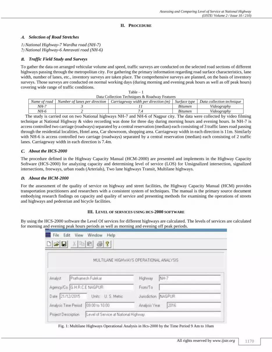
By using the HCS-2000 software the Level Of services for different highways are calculated. The levels of services are calculated

for morning and evening peak hours periods as well as morning and evening off peak periods.

Fig. 1: Multilane Highways Operational Analysis in Hcs-2000 by the Time Period 9 Am to 10am



1171

Fig. 2: Result of Multilane Highways Operational Analysis in Hcs-2000 by the Time Period 9 Am To 10am



1172

Table – 2

Flow, Density and Level of Service for Nh-7 (Morning Zone)

Time Flow (pc/h/l) Density (pc/km/h) Level of Service

Day 1 Day 2 Day 3 Day 1 Day 2 Day 3 Day 1 Day 2 Day 3

09 to 10 573 536 567 8.2 7.7 8.1 B B B

10 to 11 718 710 711 10.3 10.1 10.2 B B B

11 to 12 826 864 882 11.8 12.3 12.6 C C C

12 to 01 740 718 764 10.6 10.3 10.9 B B B

Table – 3

Flow, Density and Level of Service for Nh-7 (Evening Zone)



04 to 05 742 711 702 10.6 10.2 10.0 B B B

05 to 06 758 756 780 10.8 10.8 11.1 B B C

06 to 07 918 910 890 13.1 13.0 12.7 C C C

Table – 4

Flow, Density and Level of Service for Nh-6 (Morning Zone)



08 to 09 472 419 437 6.7 6.0 6.2 A A A

09 to 10 681 684 677 9.7 9.8 9.7 B B B

10 to 11 635 655 681 9.1 9.4 9.7 B B B

11 to 12 335 344 348 4.8 4.9 5.0 A A A

Table – 5

Flow, Density and Level of Service for Nh-6 (Evening Zone)



03 to 04 314 336 310 4.5 4.8 4.4 A A A

04 to 05 439 442 457 6.3 6.3 6.5 A A A

05 to 06 607 606 629 8.7 8.7 9.0 B B B

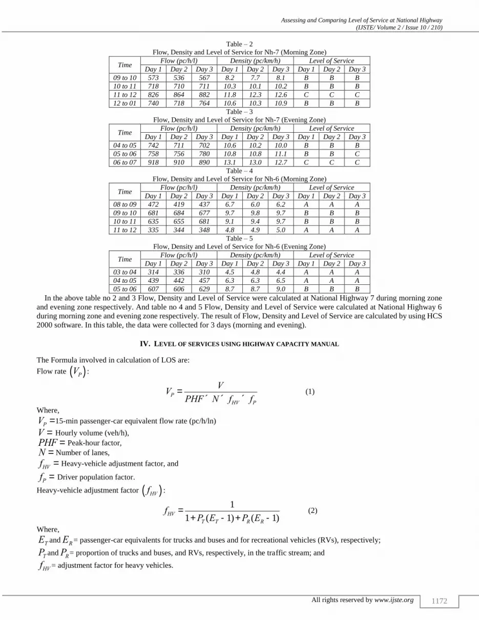
In the above table no 2 and 3 Flow, Density and Level of Service were calculated at National Highway 7 during morning zone

and evening zone respectively. And table no 4 and 5 Flow, Density and Level of Service were calculated at National Highway 6

during morning zone and evening zone respectively. The result of Flow, Density and Level of Service are calculated by using HCS

2000 software. In this table, the data were collected for 3 days (morning and evening).

IV. LEVEL OF SERVICES USING HIGHWAY CAPACITY MANUAL

The Formula involved in calculation of LOS are:

Flow rate VP( ) :

VP =V

PHF ´N ´ fHV ´ fP (1)

Where,

VP =15-min passenger-car equivalent flow rate (pc/h/ln)

V = Hourly volume (veh/h),

PHF = Peak-hour factor,

N = Number of lanes,

fHV = Heavy-vehicle adjustment factor, and

fP = Driver population factor.

Heavy-vehicle adjustment factor fHV( ) :

fHV =1

1+PT (ET -1)+PR(ER -1) (2)

Where,

ET andER= passenger-car equivalents for trucks and buses and for recreational vehicles (RVs), respectively;

PT andPR= proportion of trucks and buses, and RVs, respectively, in the traffic stream; and

fHV= adjustment factor for heavy vehicles.



1173

Free Flow speed FFS( ) :

FFS = BFFS- fLW - fLC - fM - fA (3)

Where,

FFS = free flow speed (km/h),

BFFS = base free flow speed (km/h),

fLW = Adjustment for lane width (km/h),

fLC = Adjustment for right shoulder clearance (km/h),

fN = Adjustment for number of lanes (km/h),

fID = Adjustment for interchange density (km/h).

Density D( ) :

D =VP

S (4)

Where,

D= Density (pc/km/ln),

VP = Flow rate (pc/h/ln),

S = Average passenger car speed (km/h).

According to manual, these are the required input data for Multilane Highways: Table – 6

Required Input Data for Multilane Highways Required Data Default

Geometric Data

Number of Lane -

Lane width 3.6 m

Lateral clearance 1.8 m

Median (Yes/no) -

Access-point density Exhibit 12-4

Specific grade or general terrain Level

Demand

Length of analysis period 15 min

PHF 0.85 rural, 0.90 urban

Heavy vehicles (%) 10% rural, 5% urban

Driver population factor 1.00

Calculation for NH-7 (Day 1) 9 am to 10 am,

Volume = 1507 veh/hr.

Step 1:

Step 2:

Step 3:

fHV =1

1+PT (ET -1)+PR (ER -1)

fHV =1

1+ 0.05(1.5-1)+ 0

fHV = 0.975

VP =V

PHF ´N ´ fHV ´ fP

VP =1507

0.90 ´3´ 0.975´1

VP = 572.45pc / h / ln

FFS = BFFS - fLW - fLC - fM - fA

FFS = 70 - 0 - 0

FFS = 70km / hr



1174

Step 4:

Step 5:

Determination of LOS with the value of Density,

LOS = B

In this calculation,Heavy vehice adjustment factor fHV( ) has been calculated. After that flow rate VP( ) has been calculated by

putting the value of Heavy-vehicle adjustment factor in the formula. With the data, Free Flow speed FFS( ) has been calculated.

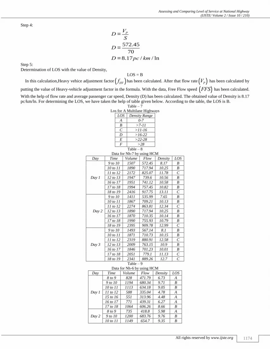
With the help of flow rate and average passenger car speed, Density (D) has been calculated. The obtained value of Density is 8.17

pc/km/ln. For determining the LOS, we have taken the help of table given below. According to the table, the LOS is B. Table – 7

Los for A Multilane Highways LOS Density Range

A 0-7

B >7-11

C >11-16

D >16-22

E >22-28

F >28

Table – 8

Data for Nh-7 by using HCM

Day Time Volume Flow Density LOS

Day 1

9 to 10 1507 572.45 8.17 B

10 to 11 1890 717.94 10.25 B

11 to 12 2172 825.07 11.78 C

12 to 13 1947 739.6 10.56 B

16 to 17 1951 741.12 10.58 B

17 to 18 1994 757.45 10.82 B

18 to 19 2416 917.75 13.11 C

Day 2

9 to 10 1411 535.99 7.65 B

10 to 11 1867 709.21 10.13 B

11 to 12 2274 863.81 12.34 C

12 to 13 1890 717.94 10.25 B

16 to 17 1870 710.35 10.14 B

17 to 18 1990 755.93 10.79 B

18 to 19 2395 909.78 12.99 C

Day 3

9 to 10 1493 567.14 8.1 B

10 to 11 1871 710.73 10.15 B

11 to 12 2319 880.91 12.58 C

12 to 13 2009 763.15 10.9 B

16 to 17 1846 701.23 10.01 B

17 to 18 2051 779.1 11.13 C

18 to 19 2341 889.26 12.7 C

Table – 9

Data for Nh-6 by using HCM Day Time Volume Flow Density LOS

Day 1

8 to 9 828 471.79 6.73 A

9 to 10 1194 680.34 9.71 B

10 to 11 1113 634.18 9.05 B

11 to 12 588 335.04 4.78 A

15 to 16 551 313.96 4.48 A

16 to 17 771 439.31 6.27 A

17 to 18 1064 606.26 8.66 B

Day 2

8 to 9 735 418.8 5.98 A

9 to 10 1200 683.76 9.76 B

10 to 11 1149 654.7 9.35 B

D =VP

S

D =572.45

70

D = 8.17pc / km / ln



1175

11 to 12 603 343.58 4.9 A

15 to 16 590 336.18 4.8 A

16 to 17 775 441.59 6.3 A

17 to 18 1063 605.69 8.65 B

Day 3

8 to 9 766 436.46 6.23 A

9 to 10 1187 676.35 9.66 B

10 to 11 1195 680.91 9.72 B

11 to 12 611 348.14 4.97 A

15 to 16 544 309.97 4.42 A

16 to 17 801 456.41 6.52 A

17 to 18 1104 629.05 8.98 B

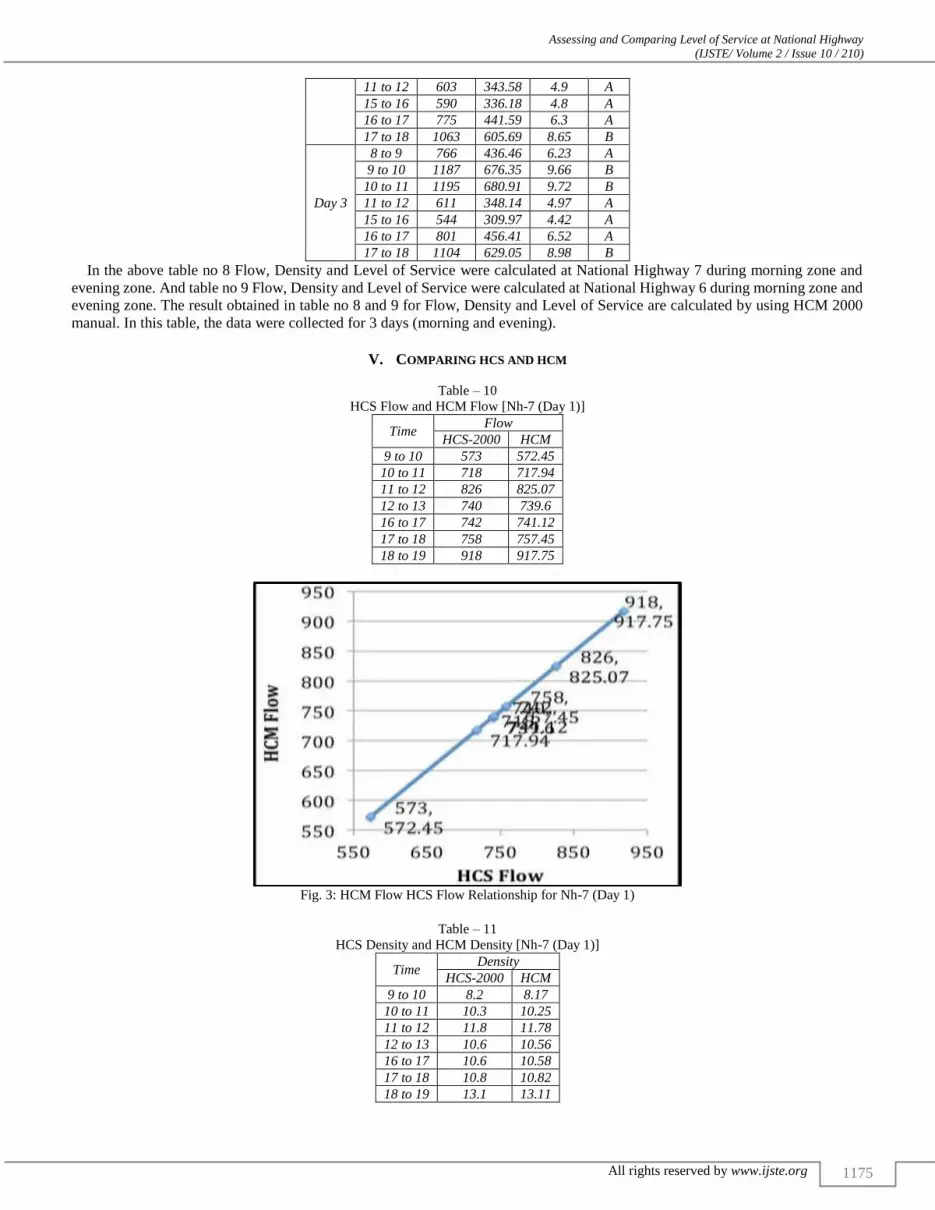
In the above table no 8 Flow, Density and Level of Service were calculated at National Highway 7 during morning zone and

evening zone. And table no 9 Flow, Density and Level of Service were calculated at National Highway 6 during morning zone and

evening zone. The result obtained in table no 8 and 9 for Flow, Density and Level of Service are calculated by using HCM 2000

manual. In this table, the data were collected for 3 days (morning and evening).

V. COMPARING HCS AND HCM

Table – 10

HCS Flow and HCM Flow [Nh-7 (Day 1)]

Time Flow

HCS-2000 HCM

9 to 10 573 572.45

10 to 11 718 717.94

11 to 12 826 825.07

12 to 13 740 739.6

16 to 17 742 741.12

17 to 18 758 757.45

18 to 19 918 917.75

Fig. 3: HCM Flow HCS Flow Relationship for Nh-7 (Day 1)

Table – 11

HCS Density and HCM Density [Nh-7 (Day 1)]

Time Density

HCS-2000 HCM

9 to 10 8.2 8.17

10 to 11 10.3 10.25

11 to 12 11.8 11.78

12 to 13 10.6 10.56

16 to 17 10.6 10.58

17 to 18 10.8 10.82

18 to 19 13.1 13.11



1176

Fig. 4: HCM Density HCS Density Relationship for Nh-7 (Day 1)

Table – 12

HCS Los and HCM Los [Nh-7 (Day 1)]

Time LOS

HCS-2000 HCM

9 to 10 B B

10 to 11 B B

11 to 12 C C

12 to 13 B B

16 to 17 B B

17 to 18 B B

18 to 19 C C

In these above table and figure, comparison has been done between HCS software and HCM manual. In table no 10; the flow

has been compare between HCS and HCM for NH-7 day 1.In figure 3, graph has been drawn showing comparison between HCS

Flow and HCM flow. Similarly, for table 11 and figure 4 Density has been compared. In table 12, it has been observed that the

LOS value is similar for manual and software. Table – 13

HCS Flow and HCM Flow [Nh-6 (Day 1)]

Time Flow

HCS-2000 HCM

8 to 9 472 471.79

9 to 10 681 680.34

10 to 11 635 634.18

11 to 12 335 335.04

15 to 16 314 313.96

16 to 17 439 439.31

17 to 18 607 606.26

Fig. 5: HCM Flow HCS Flow Relationship for Nh-6 (Day 1)



1177

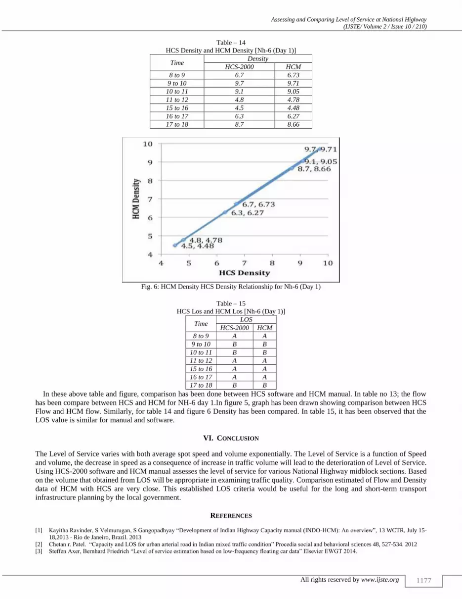
Table – 14

HCS Density and HCM Density [Nh-6 (Day 1)]

Time Density

HCS-2000 HCM

8 to 9 6.7 6.73

9 to 10 9.7 9.71

10 to 11 9.1 9.05

11 to 12 4.8 4.78

15 to 16 4.5 4.48

16 to 17 6.3 6.27

17 to 18 8.7 8.66

Fig. 6: HCM Density HCS Density Relationship for Nh-6 (Day 1)

Table – 15

HCS Los and HCM Los [Nh-6 (Day 1)]

Time LOS

HCS-2000 HCM

8 to 9 A A

9 to 10 B B

10 to 11 B B

11 to 12 A A

15 to 16 A A

16 to 17 A A

17 to 18 B B

In these above table and figure, comparison has been done between HCS software and HCM manual. In table no 13; the flow

has been compare between HCS and HCM for NH-6 day 1.In figure 5, graph has been drawn showing comparison between HCS

Flow and HCM flow. Similarly, for table 14 and figure 6 Density has been compared. In table 15, it has been observed that the

LOS value is similar for manual and software.

VI. CONCLUSION

The Level of Service varies with both average spot speed and volume exponentially. The Level of Service is a function of Speed

and volume, the decrease in speed as a consequence of increase in traffic volume will lead to the deterioration of Level of Service.

Using HCS-2000 software and HCM manual assesses the level of service for various National Highway midblock sections. Based

on the volume that obtained from LOS will be appropriate in examining traffic quality. Comparison estimated of Flow and Density

data of HCM with HCS are very close. This established LOS criteria would be useful for the long and short-term transport

infrastructure planning by the local government.

REFERENCES

[1] Kayitha Ravinder, S Velmurugan, S Gangopadhyay “Development of Indian Highway Capacity manual (INDO-HCM): An overview”, 13 WCTR, July 15-

18,2013 - Rio de Janeiro, Brazil. 2013

[2] Chetan r. Patel. “Capacity and LOS for urban arterial road in Indian mixed traffic condition” Procedia social and behavioral sciences 48, 527-534. 2012 [3] Steffen Axer, Bernhard Friedrich “Level of service estimation based on low-frequency floating car data” Elsevier EWGT 2014.



1178

[4] Marta R. Obelheiro, Helena B. B. Cybis, Jose L. D. Ribeiro “ Level of Service Method for Brazilian Toll Plazas “, Procedia Social and Behavioral Sciences

16 (2011) 120–130. [5] Ganesh M. Pawar “Assessing Level of Service For Highways In a New Metropolitan City Using HCS-2000”. 2015

[6] Steffen Axer, Jannis Rohde, Bernhard Friedrich “Level of service estimation at traffic signals based on innovative traffic data services and collection

techniques” Elsevier EWGT 2012. [7] Johan Olstam, Andreas Tapani “A Review of Guidelines for Applying Traffic Simulation to Level-of-service Analysis” Elsevier 2011.

[8] Eleonora Papadimitriou, Varvara Mylona, John Golias “Perceived Level of Service, Driver, and Traffic Characteristics: Piecewise Linear Model” JOURNAL

OF TRANSPORTATION ENGINEERING © ASCE / OCTOBER 2010 [9] Feng-Bor Lin, Chang-Wei SU, Hsin-Hsiun Huang “Uniform Criteria for Level of Service analysis of Freeways” JOURNAL OF TRANSPORTATION

ENGINEERING / MARCH/APRIL 1996

assessing and comparing level of service at national highway

Documents