applied metal forming: including fem analysis
TRANSCRIPT


This page intentionally left blank
APPLIED METAL FORMINGIncluding FEM Analysis
Applied Metal Forming: Including FEM Analysis describes metalforming theory and how experimental techniques can be used tostudy metal forming operations with great accuracy. For each primaryclass of processes, such as forging, rolling, extrusion, wiredrawing, andsheet-metal forming, it explains how finite element analysis (FEA) canbe applied with great precision to characterize the forming conditionsand in this way optimize the processes. FEA has made it possible tobuild realistic FEM models of most metal forming processes, includ-ing complex three-dimensional forming operations, in which complexproducts are shaped by complex dies. Thus, using FEA, it is now pos-sible to visualize any metal forming process and to study strain, stress,and other forming conditions inside the parts being manufactured asthey develop throughout the process.
Henry S. Valberg is a professor in the Department of Engineering Sci-ence and Materials at the Norwegian University of Science and Tech-nology (NTNU). He began his professional career as a metallurgist atthe Royal Norwegian Air Force (LFK), and continued it at A/S NorskJernverk, Mo i Rana, and then as a research scientist at SINTEF, Divi-sion of Materials and Processes, before joining the Norwegian Instituteof Technology (NTH) as a senior lecturer in 1984 and full professor in1994. He was a visiting professor at Denmark’s Technical Universityin 1997–1998. Professor Valberg’s main fields of research are materi-als, metal forming, experimental deformation analysis, and FEA. Hiswork covers all the main metal forming processes, including forging,rolling, extrusion, drawing, and sheet-metal forming. He is the authorof more than 60 refereed journal articles and has supervised numerousgraduate students. Professor Valberg is currently a research managerin a project run by three Norwegian forging companies.


Applied Metal Forming
INCLUDING FEM ANALYSIS
Henry S. ValbergNorwegian University of Science and Technology

CAMBRIDGE UNIVERSITY PRESS
Cambridge, New York, Melbourne, Madrid, Cape Town, Singapore,
São Paulo, Delhi, Dubai, Tokyo
Cambridge University Press
The Edinburgh Building, Cambridge CB2 8RU, UK
First published in print format
ISBN-13 978-0-521-51823-9
ISBN-13 978-0-511-72943-0
© Henry Valberg 2010
2010
Information on this title: www.cambridge.org/9780521518239
This publication is in copyright. Subject to statutory exception and to the
provision of relevant collective licensing agreements, no reproduction of any part
may take place without the written permission of Cambridge University Press.
Cambridge University Press has no responsibility for the persistence or accuracy
of urls for external or third-party internet websites referred to in this publication,
and does not guarantee that any content on such websites is, or will remain,
accurate or appropriate.
Published in the United States of America by Cambridge University Press, New York
www.cambridge.org
eBook (NetLibrary)
Hardback
Contents
Preface page vii
1 Characteristics of Metal Forming . . . . . . . . . . . . . . . . . . . . . . . . . . . . 1
2 Important Metal Forming Processes . . . . . . . . . . . . . . . . . . . . . . . . . 18
3 FEA of Metal Forming . . . . . . . . . . . . . . . . . . . . . . . . . . . . . . . . . . . 34
4 Theory . . . . . . . . . . . . . . . . . . . . . . . . . . . . . . . . . . . . . . . . . . . . . . 53
5 Reduction and Proportions of the Plastic Zone . . . . . . . . . . . . . . . . . 77
6 Deformations from the Velocity Field . . . . . . . . . . . . . . . . . . . . . . . . 84
7 Technological Tests and Physical Simulation . . . . . . . . . . . . . . . . . . . 92
8 Flow Stress Data . . . . . . . . . . . . . . . . . . . . . . . . . . . . . . . . . . . . . . 115
9 Formability and Workability . . . . . . . . . . . . . . . . . . . . . . . . . . . . . . 127
10 Friction and Friction Models . . . . . . . . . . . . . . . . . . . . . . . . . . . . . . 139
11 Thermal Effects . . . . . . . . . . . . . . . . . . . . . . . . . . . . . . . . . . . . . . . 159
12 Experimental Metal Flow Analysis . . . . . . . . . . . . . . . . . . . . . . . . . 181
13 Theoretical Methods of Analysis . . . . . . . . . . . . . . . . . . . . . . . . . . . 204
14 Finite Element Analysis . . . . . . . . . . . . . . . . . . . . . . . . . . . . . . . . . 219
15 FEA of Technological Tests . . . . . . . . . . . . . . . . . . . . . . . . . . . . . . 242
16 Forging . . . . . . . . . . . . . . . . . . . . . . . . . . . . . . . . . . . . . . . . . . . . . 268
17 FEA of Forging . . . . . . . . . . . . . . . . . . . . . . . . . . . . . . . . . . . . . . . 285
v

vi Contents
18 Extrusion . . . . . . . . . . . . . . . . . . . . . . . . . . . . . . . . . . . . . . . . . . . . 320
19 FEA of Extrusion . . . . . . . . . . . . . . . . . . . . . . . . . . . . . . . . . . . . . . 347
20 Rolling . . . . . . . . . . . . . . . . . . . . . . . . . . . . . . . . . . . . . . . . . . . . . 365
21 FEA of Rolling . . . . . . . . . . . . . . . . . . . . . . . . . . . . . . . . . . . . . . . 376
22 Drawing of Wire, Profiles, and Tubes . . . . . . . . . . . . . . . . . . . . . . . . 395
23 FEA of Wiredrawing . . . . . . . . . . . . . . . . . . . . . . . . . . . . . . . . . . . 414
24 Sheet-Metal Forming . . . . . . . . . . . . . . . . . . . . . . . . . . . . . . . . . . . 435
25 FEA of Sheet-Metal Forming (Available atwww.cambridge.org/valberg) . . . . . . . . . . . . . . . . . . . . . . . . . . . . . . . .
Index 453

Preface
Finite element analysis (FEA) has currently been developed into an efficient, user-friendly tool for investigation of metal forming processes. At the same time, cheap,efficient computers have been developed that allow simulation of metal forming tobe done by use of the finite element method (FEM), within reasonable times. Thisrecent development is, as this book will show, about to revolutionize the art of metalforming.
This technology has made it possible to build realistic FEM models of perhapsany metal forming process, including complex three-dimensional forming opera-tions, in which complex products are shaped by means of complex dies. Thus, byFEA, it is now possible to visualize any metal forming process on the computerscreen and to study strain, stress, and other important forming conditions inside theworkpiece, as they develop throughout the duration of the process. Because of this,FEA has also become an important industrial tool in connection with developmentand design of new metal forming processes.
However, in spite of this development, there is still need for classical theory asa tool for providing knowledge about forming. For a person to be able to utilize thenew FEA technology and to evaluate the results obtained in FEA, it is required thathe or she have deep insight into the theory of metal forming.
In order to establish correct FEM models, it is still required to investigate metalforming by means of experiments performed in the laboratory or on industrialequipment. Without some experimentation, it is difficult to know what informationshould be fed into the FEM model, and to what extent a simulation is precise. Ifinput data to the model is wrong, the usefulness of FEA may be limited.
Throughout his career, the author of this book has done much work to developnew visioplasticity methods for the study of metal flow in metal forming. In thisway, a new advanced grid pattern technique has been developed, which allows stripepatterns to be made in the interior of a workpiece and ring patterns to be addedonto its surface, to be shaped later by metal forming. These techniques are useful inthat they allow precise characterization of metal flow, inside and on the surface of aworkpiece.
vii

viii Preface
The book describes metal forming theory briefly and explains how experimen-tal techniques can be used to study the forming conditions of metal forming oper-ations with great accuracy. In addition, it is shown for each of the main classes ofmetal forming processes – forging, rolling, extrusion, wiredrawing, and sheet-metalforming – how FEA can be applied precisely to characterize forming conditions inthese operations, and in this way optimize the processes.
Examples are provided throughout the book to illustrate how theory, experi-ments, and FEA in combination can be used to calculate and characterize the con-ditions in a forming process. In each chapter, a number of illustrative problems areprovided. A solution manual will be provided separately.
The chapters dealing with FEA have been written so that it is not requiredfor the reader to apply a FEM program. Simulation results are presented, and thereader will gain experience in evaluation of postprocessing data from FEM models.However, the best situation for the reader will, of course, be if he or she has accessto a FEM simulation program and hence can rerun or modify some of the FEMmodels presented in the book.
The book is applicable on both the undergraduate and graduate levels in uni-versities and should also be useful for the metal-former working in industry.
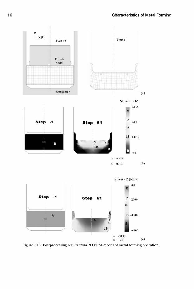
In addition to the book’s printed content, additional materials have been madeavailable on the Web site www.cambridge.org/valberg. A full chapter on FEA ofsheet-metal is available for free review or download. Also available are color repre-sentations of many of the book figures designed to enhance the reader’s understand-ing. In the gray-scale figures, letters have been used to indicate color distribution asfollows: R = red, Y = yellow, G = green, LB = light blue, B = blue.
I would like to thank Dr. Dirk Nolte and Dr. Rama Krishna Uyyuru, who haveread through the manuscript and proposed improvements. Thanks are also due tomy current and former students, most of them on the master’s level, who haveworked with the topics covered by the book. I would also like to thank my homeuniversity (NTNU) for providing financial support for two sabbaticals. The FEApart of the book could not have been realized without this support.
Finally, I would like to express thanks to my wife, Beate Linge, for her patienceduring the time required for writing this book.
Trondheim, January 25, 2010

APPLIED METAL FORMING

1 Characteristics of Metal Forming
Metal forming is one manufacturing method among many. In order to manufacturea machine component, such as a wheel suspension arm for a car, one can choosemetal forming, casting, or machining as the shaping method. These three shapingmethods can be considered competing processes. The method chosen will usually bethe one that provides a product, with proper function and properties, at the lowestcost. In this chapter, characteristics of these three shaping methods will be described,with special emphasis on metal forming, when used to create the intended shape ofa component through plastic deformations of an initial workpiece of simple shape.
1.1 Definition of Metal Forming
Metal forming refers to shaping of metallic materials by means of plastic defor-mation. The term plastic deformation describes permanent shape change, in con-trast to elastic deformation. An elastic deformation disappears when the load isremoved. Many industrial materials are shaped into useful products by plastic defor-mation. Clay is a material that is shaped by plastic deformation before it is fired tobecome a final useful solid ceramic material. In addition, polymer materials are com-monly shaped in melted condition by means of plastic deformation. But in this book,the treatment is confined to plastic deformation of metals.
A more comprehensive definition of metal forming is the technology used forshaping metal alloys into useful products by forming processes such as rolling, forg-ing, extrusion, drawing, and sheet-metal forming. With this definition, the terminvolves many scientific disciplines, including chemistry, physics, mechanics, andgeneral manufacturing technology.
1.2 Plastic Deformations on Micro- and Macroscopic Scales
The term plastic deformation can be explained if one examines a metallic materialthat is subjected to deformation in a specific metal forming process.
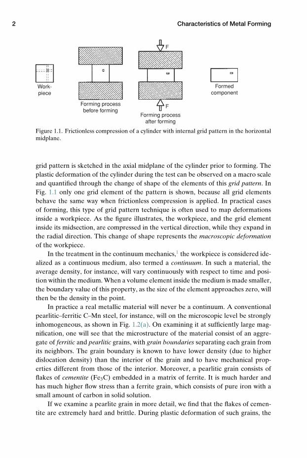
Figure 1.1 shows the frictionless compression of a cylinder between two parallelplatens as either a cold- or a hot-forming process. An area element from an internal
1
2 Characteristics of Metal Forming
Work-piece
Forming processbefore forming
Forming processafter forming
Formedcomponent
F
F
Figure 1.1. Frictionless compression of a cylinder with internal grid pattern in the horizontalmidplane.
grid pattern is sketched in the axial midplane of the cylinder prior to forming. Theplastic deformation of the cylinder during the test can be observed on a macro scaleand quantified through the change of shape of the elements of this grid pattern. InFig. 1.1 only one grid element of the pattern is shown, because all grid elementsbehave the same way when frictionless compression is applied. In practical casesof forming, this type of grid pattern technique is often used to map deformationsinside a workpiece. As the figure illustrates, the workpiece, and the grid elementinside its midsection, are compressed in the vertical direction, while they expand inthe radial direction. This change of shape represents the macroscopic deformationof the workpiece.
In the treatment in the continuum mechanics,1 the workpiece is considered ide-alized as a continuous medium, also termed a continuum. In such a material, theaverage density, for instance, will vary continuously with respect to time and posi-tion within the medium. When a volume element inside the medium is made smaller,the boundary value of this property, as the size of the element approaches zero, willthen be the density in the point.
In practice a real metallic material will never be a continuum. A conventionalpearlitic–ferritic C–Mn steel, for instance, will on the microscopic level be stronglyinhomogeneous, as shown in Fig. 1.2(a). On examining it at sufficiently large mag-nification, one will see that the microstructure of the material consist of an aggre-gate of ferritic and pearlitic grains, with grain boundaries separating each grain fromits neighbors. The grain boundary is known to have lower density (due to higherdislocation density) than the interior of the grain and to have mechanical prop-erties different from those of the interior. Moreover, a pearlitic grain consists offlakes of cementite (Fe3C) embedded in a matrix of ferrite. It is much harder andhas much higher flow stress than a ferrite grain, which consists of pure iron with asmall amount of carbon in solid solution.
If we examine a pearlite grain in more detail, we find that the flakes of cemen-tite are extremely hard and brittle. During plastic deformation of such grains, the

1.2 Plastic Deformations on Micro- and Macroscopic Scales 3
(a) (b)
Cementiteflakes
Edgedislocations
Prior to deformation: Small plasticdeformation:
Large plasticdeformation:
h0h1
h
Densely packedcrystal planes
Grain of pearlite
(α+Fe3C)
Grain offerrite(α)
Dislocationtangles
Fracturedflakes
(c)
Figure 1.2. Schematic sketch showing micro-scale effects of plastic deformation in pearlitic–ferritic steel: (a) undeformed grains, (b) deformation of ferrite by dislocation movement, (c)multiplication of dislocations in ferrite and fracture of cementite flakes in pearlite.
ferrite, in which the brittle flakes are embedded, deforms severely by microscopicplastic deformation. The flakes themselves, because of their low ductility, fractureinto small pieces; see Fig. 1.2(c). The reason the pearlitic grains can deform plasti-cally without damaging the whole microstructure is the distribution of the cementiteflakes as small islands in the more ductile ferrite matrix.
Cast irons, which contain much more carbon than steel (>1.7% C), sometimescan form a microstructure in which films of cementite appear as a continuous skele-ton throughout the grain boundaries of the whole material. The materials in thisstate are very brittle and cannot be deformed plastically without fracture. If, forexample, one tries to bend a component of such a material, to change its shape per-manently, it will fracture before it is plasticized. This illustrates that on a micro scalea metallic material commonly consists of different phases with different mechanicalproperties. Moreover, most metallic materials will consist of an aggregate of crystalgrains. In the grains, the atoms are packed along various crystallographic planes.The orientation of the crystal planes will be different from one grain to a neighbor-ing grain. Because these inhomogeneities are of small size, commonly < 100 µm, thematerial can, anyhow on a macroscopic level, be considered a continuum and canbe well described by the theory of continuum mechanics.
When considered on a sufficiently small scale, so that atoms become visible,plastic deformation of metals is known to be caused by dislocations. They are gener-ated in the metal upon plastic deformation and move through the grains, along thedensely packed atomic planes of the microstructure, as shown in Fig. 1.2(b,c) andFig. 1.3. New dislocations are also formed during cold forming, so that the disloca-tion density increases as the metal is subjected to larger strains.
However, plastic deformation in melted polymers and in clay occurs by mech-anisms different from those in metals. In polymers, sliding of long polymer chainsagainst one another is the most common mechanism of plastic deformation. In clays,
4 Characteristics of Metal Forming
Edge dislocation slidingthrough the crystal
Perfect atomiccrystal structure
Plastic deformationdue to passage ofdislocation through
the crystal
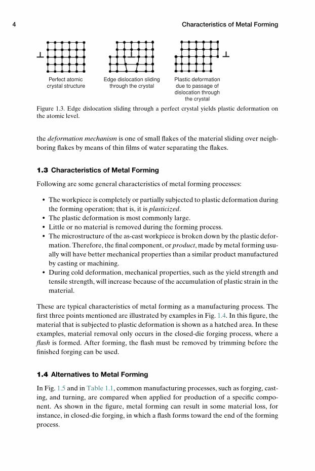
Figure 1.3. Edge dislocation sliding through a perfect crystal yields plastic deformation onthe atomic level.
the deformation mechanism is one of small flakes of the material sliding over neigh-boring flakes by means of thin films of water separating the flakes.
1.3 Characteristics of Metal Forming
Following are some general characteristics of metal forming processes:
� The workpiece is completely or partially subjected to plastic deformation duringthe forming operation; that is, it is plasticized.
� The plastic deformation is most commonly large.� Little or no material is removed during the forming process.� The microstructure of the as-cast workpiece is broken down by the plastic defor-
mation. Therefore, the final component, or product, made by metal forming usu-ally will have better mechanical properties than a similar product manufacturedby casting or machining.
� During cold deformation, mechanical properties, such as the yield strength andtensile strength, will increase because of the accumulation of plastic strain in thematerial.
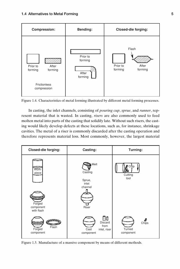
These are typical characteristics of metal forming as a manufacturing process. Thefirst three points mentioned are illustrated by examples in Fig. 1.4. In this figure, thematerial that is subjected to plastic deformation is shown as a hatched area. In theseexamples, material removal only occurs in the closed-die forging process, where aflash is formed. After forming, the flash must be removed by trimming before thefinished forging can be used.
1.4 Alternatives to Metal Forming
In Fig. 1.5 and in Table 1.1, common manufacturing processes, such as forging, cast-ing, and turning, are compared when applied for production of a specific compo-nent. As shown in the figure, metal forming can result in some material loss, forinstance, in closed-die forging, in which a flash forms toward the end of the formingprocess.
1.4 Alternatives to Metal Forming 5
Afterforming
Afterforming
Flash
Closed-die forging:Bending:Compression:
Afterforming
Prior toforming
Prior toforming
Prior toforming
Frictionlesscompression
Figure 1.4. Characteristics of metal forming illustrated by different metal forming processes.
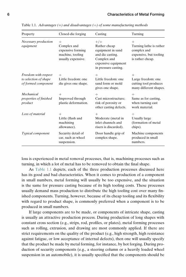
In casting, the inlet channels, consisting of pouring cup, sprue, and runner, rep-resent material that is wasted. In casting, risers are also commonly used to feedmolten metal into parts of the casting that solidify late. Without such risers, the cast-ing would likely develop defects at these locations, such as, for instance, shrinkagecavities. The metal of a riser is commonly discarded after the casting operation andtherefore represents material loss. Most commonly, however, the largest material
Closed-die forging: Casting: Turning:
Forgedcomponentwith flash
Forgedcomponent
Castcomponent
Turnedcomponent
Flash
Riser
Discardfrom
inlet, riser
Chips
CastingWork-piece
Melt
Cuttingtool
Chip
Sprue,inlet
channel
Figure 1.5. Manufacture of a massive component by means of different methods.
6 Characteristics of Metal Forming
Table 1.1. Advantages (+) and disadvantages (÷) of some manufacturing methods
Property Closed-die forging Casting Turning
Necessary productionequipment
÷ +/÷ +Complex andexpensive formingmachine, toolingusually expensive.
Rather cheapequipment in sandand die casting.Complex andexpensive equipmentin pressure casting.
Turning lathe is rathercomplex andexpensive, but toolingis rather cheap.
Freedom with respectto selection of shapeof formed component
÷ ÷ +Little freedom: onedie gives one shape.
Little freedom: onesand form or moldgives one shape.
Large freedom: onecutting tool producesmany different shapes.
Mechanicalproperties of finishedproduct
+ ÷ ÷Improved throughplastic deformation.
Cast microstructure;risk of porosity orother casting defects.
Same as for casting,when turning castwork material.
Loss of material + + ÷Little (flash andmachiningallowance).
Moderate (metal ininlet channels andrisers is discarded).
Usually large(formation of metalchips).
Typical component Security detail ofcar, such as wheelsuspension.
Door handle grip ofcomplex shape.
Machine componentsproduced in smallnumbers.
loss is experienced in metal removal processes, that is, machining processes such asturning, in which a lot of metal has to be removed to obtain the final shape.
As Table 1.1 depicts, each of the three production processes discussed herehas its good and bad characteristics. When it comes to production of a componentin small numbers, metal forming will usually be too expensive, and the situationis the same for pressure casting because of its high tooling costs. These processesusually demand mass production to distribute the high tooling cost over many fin-ished components. Turning, however, because of its cheap tooling and its flexibilitywith regard to product shape, is commonly preferred when a component is to beproduced in small numbers.
If large components are to be made, or components of intricate shape, castingis usually an attractive production process. During production of long shapes withconstant cross section (e.g., strips, rod, profiles, or plates), metal forming processessuch as rolling, extrusion, and drawing are most commonly applied. If there arestrict requirements on the quality of the product (e.g., high strength, high resistanceagainst fatigue, or low acceptance of internal defects), then one will usually specifythat the product be made by metal forming, for instance, by hot forging. During pro-duction of security components (e.g., a steering column or a heavily loaded wheelsuspension in an automobile), it is usually specified that the components should be
1.5 Change of Properties Due to Plastic Working 7
Elo
ng
atio
n a
t fr
actu
re(%
)
Reduction(%)
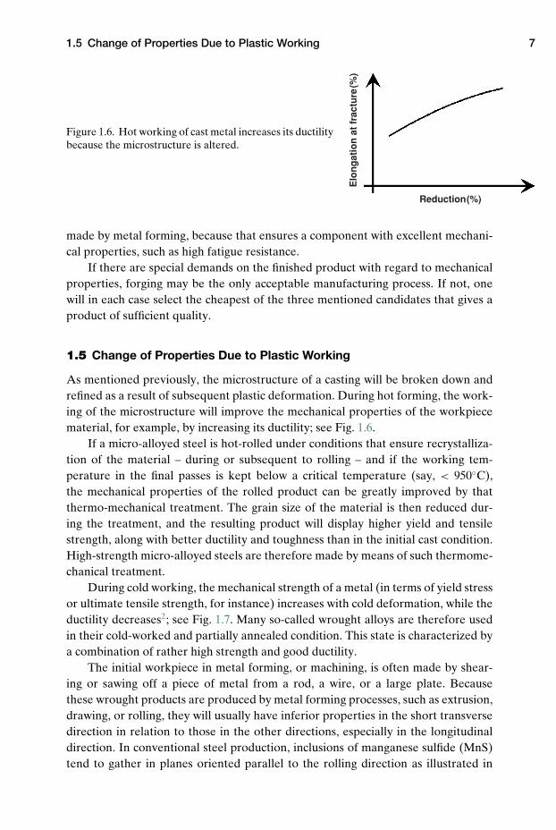
Figure 1.6. Hot working of cast metal increases its ductilitybecause the microstructure is altered.
made by metal forming, because that ensures a component with excellent mechani-cal properties, such as high fatigue resistance.
If there are special demands on the finished product with regard to mechanicalproperties, forging may be the only acceptable manufacturing process. If not, onewill in each case select the cheapest of the three mentioned candidates that gives aproduct of sufficient quality.
1.5 Change of Properties Due to Plastic Working
As mentioned previously, the microstructure of a casting will be broken down andrefined as a result of subsequent plastic deformation. During hot forming, the work-ing of the microstructure will improve the mechanical properties of the workpiecematerial, for example, by increasing its ductility; see Fig. 1.6.
If a micro-alloyed steel is hot-rolled under conditions that ensure recrystalliza-tion of the material – during or subsequent to rolling – and if the working tem-perature in the final passes is kept below a critical temperature (say, < 950◦C),the mechanical properties of the rolled product can be greatly improved by thatthermo-mechanical treatment. The grain size of the material is then reduced dur-ing the treatment, and the resulting product will display higher yield and tensilestrength, along with better ductility and toughness than in the initial cast condition.High-strength micro-alloyed steels are therefore made by means of such thermome-chanical treatment.
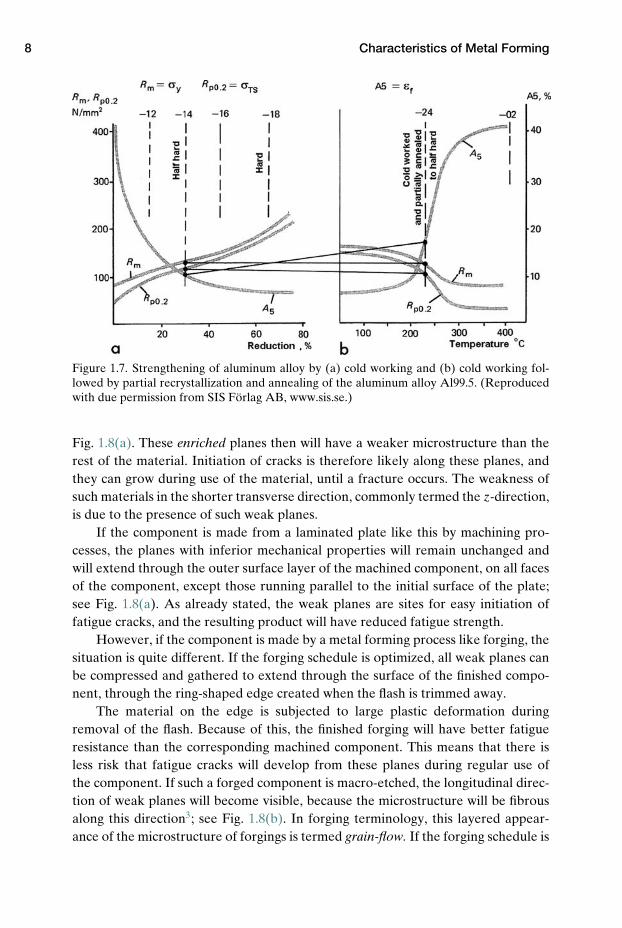
During cold working, the mechanical strength of a metal (in terms of yield stressor ultimate tensile strength, for instance) increases with cold deformation, while theductility decreases2; see Fig. 1.7. Many so-called wrought alloys are therefore usedin their cold-worked and partially annealed condition. This state is characterized bya combination of rather high strength and good ductility.
The initial workpiece in metal forming, or machining, is often made by shear-ing or sawing off a piece of metal from a rod, a wire, or a large plate. Becausethese wrought products are produced by metal forming processes, such as extrusion,drawing, or rolling, they will usually have inferior properties in the short transversedirection in relation to those in the other directions, especially in the longitudinaldirection. In conventional steel production, inclusions of manganese sulfide (MnS)tend to gather in planes oriented parallel to the rolling direction as illustrated in
8 Characteristics of Metal Forming
Figure 1.7. Strengthening of aluminum alloy by (a) cold working and (b) cold working fol-lowed by partial recrystallization and annealing of the aluminum alloy Al99.5. (Reproducedwith due permission from SIS Forlag AB, www.sis.se.)
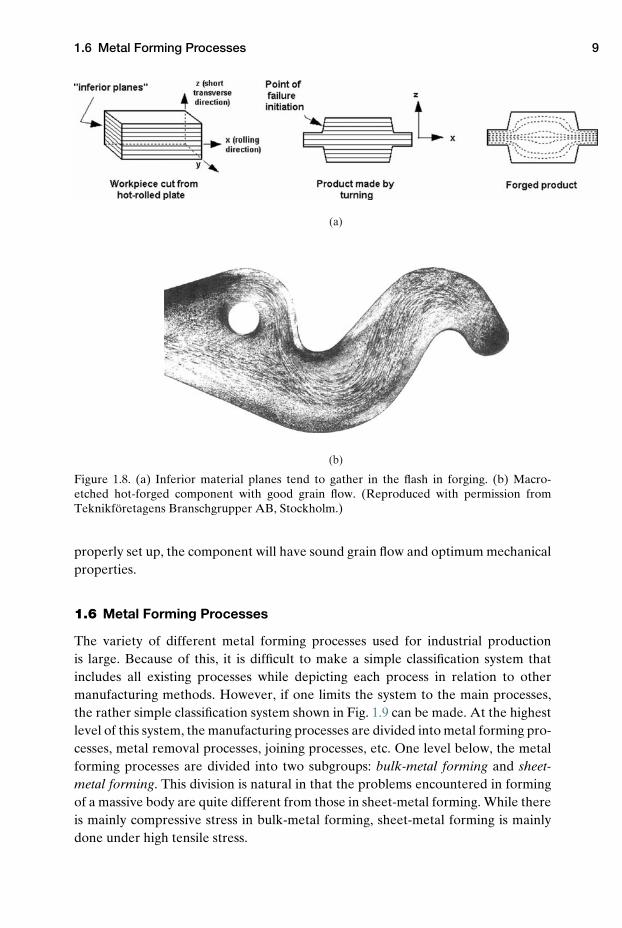
Fig. 1.8(a). These enriched planes then will have a weaker microstructure than therest of the material. Initiation of cracks is therefore likely along these planes, andthey can grow during use of the material, until a fracture occurs. The weakness ofsuch materials in the shorter transverse direction, commonly termed the z-direction,is due to the presence of such weak planes.
If the component is made from a laminated plate like this by machining pro-cesses, the planes with inferior mechanical properties will remain unchanged andwill extend through the outer surface layer of the machined component, on all facesof the component, except those running parallel to the initial surface of the plate;see Fig. 1.8(a). As already stated, the weak planes are sites for easy initiation offatigue cracks, and the resulting product will have reduced fatigue strength.
However, if the component is made by a metal forming process like forging, thesituation is quite different. If the forging schedule is optimized, all weak planes canbe compressed and gathered to extend through the surface of the finished compo-nent, through the ring-shaped edge created when the flash is trimmed away.
The material on the edge is subjected to large plastic deformation duringremoval of the flash. Because of this, the finished forging will have better fatigueresistance than the corresponding machined component. This means that there isless risk that fatigue cracks will develop from these planes during regular use ofthe component. If such a forged component is macro-etched, the longitudinal direc-tion of weak planes will become visible, because the microstructure will be fibrousalong this direction3; see Fig. 1.8(b). In forging terminology, this layered appear-ance of the microstructure of forgings is termed grain-flow. If the forging schedule is
1.6 Metal Forming Processes 9
(a)
(b)
Figure 1.8. (a) Inferior material planes tend to gather in the flash in forging. (b) Macro-etched hot-forged component with good grain flow. (Reproduced with permission fromTeknikforetagens Branschgrupper AB, Stockholm.)
properly set up, the component will have sound grain flow and optimum mechanicalproperties.
1.6 Metal Forming Processes
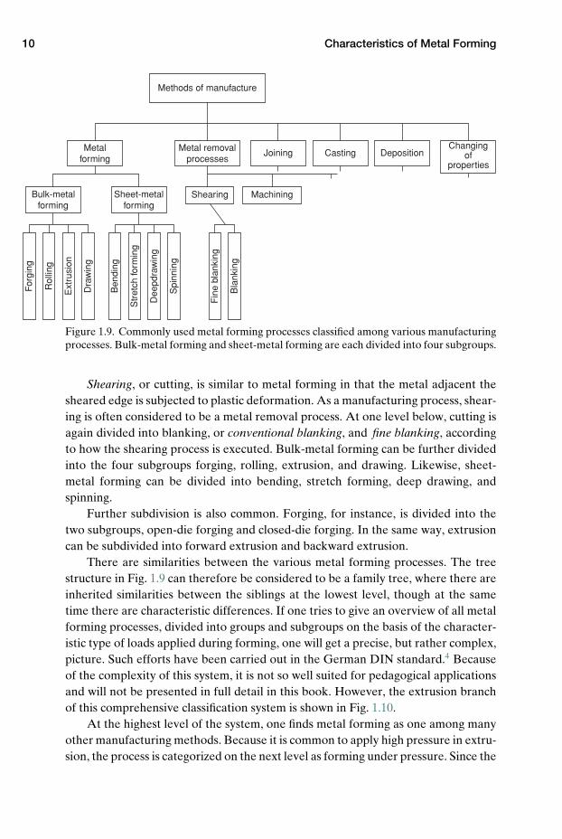
The variety of different metal forming processes used for industrial productionis large. Because of this, it is difficult to make a simple classification system thatincludes all existing processes while depicting each process in relation to othermanufacturing methods. However, if one limits the system to the main processes,the rather simple classification system shown in Fig. 1.9 can be made. At the highestlevel of this system, the manufacturing processes are divided into metal forming pro-cesses, metal removal processes, joining processes, etc. One level below, the metalforming processes are divided into two subgroups: bulk-metal forming and sheet-metal forming. This division is natural in that the problems encountered in formingof a massive body are quite different from those in sheet-metal forming. While thereis mainly compressive stress in bulk-metal forming, sheet-metal forming is mainlydone under high tensile stress.
10 Characteristics of Metal Forming
Methods of manufacture
Changingof
propertiesDepositionCastingJoining
Shearing Machining
For
ging
Rol
ling
Ext
rusi
on
Dra
win
g
Ben
ding
Str
etch
form
ing
Dee
pdra
win
g
Spi
nnin
g
Fin
e bl
anki
ng
Bla
nkin
g
Metal removalprocesses
Metalforming
Bulk-metalforming
Sheet-metalforming
Figure 1.9. Commonly used metal forming processes classified among various manufacturingprocesses. Bulk-metal forming and sheet-metal forming are each divided into four subgroups.
Shearing, or cutting, is similar to metal forming in that the metal adjacent thesheared edge is subjected to plastic deformation. As a manufacturing process, shear-ing is often considered to be a metal removal process. At one level below, cutting isagain divided into blanking, or conventional blanking, and fine blanking, accordingto how the shearing process is executed. Bulk-metal forming can be further dividedinto the four subgroups forging, rolling, extrusion, and drawing. Likewise, sheet-metal forming can be divided into bending, stretch forming, deep drawing, andspinning.
Further subdivision is also common. Forging, for instance, is divided into thetwo subgroups, open-die forging and closed-die forging. In the same way, extrusioncan be subdivided into forward extrusion and backward extrusion.
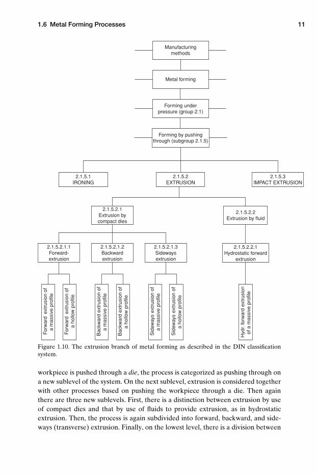
There are similarities between the various metal forming processes. The treestructure in Fig. 1.9 can therefore be considered to be a family tree, where there areinherited similarities between the siblings at the lowest level, though at the sametime there are characteristic differences. If one tries to give an overview of all metalforming processes, divided into groups and subgroups on the basis of the character-istic type of loads applied during forming, one will get a precise, but rather complex,picture. Such efforts have been carried out in the German DIN standard.4 Becauseof the complexity of this system, it is not so well suited for pedagogical applicationsand will not be presented in full detail in this book. However, the extrusion branchof this comprehensive classification system is shown in Fig. 1.10.
At the highest level of the system, one finds metal forming as one among manyother manufacturing methods. Because it is common to apply high pressure in extru-sion, the process is categorized on the next level as forming under pressure. Since the
1.6 Metal Forming Processes 11
For
war
d ex
trus
ion
ofa
mas
sive
pro
file
Bac
kwar
d ex
trus
ion
of
a m
assi
ve p
rofil
e
Hyd
r. fo
rwar
d ex
trus
ion
of a
mas
sive
pro
file
Bac
kwar
d ex
trus
ion
of
Sid
eway
s ex
trus
ion
of
Sid
eway
s ex
trus
ion
of
a m
assi
ve p
rofil
e
For
war
d ex
trus
ion
ofa
hollo
w p
rofil
e
a ho
llow
pro
file
a ho
llow
pro
file
Metal forming
Forming underpressure (group 2.1)
Forming by pushingthrough (subgroup 2.1.5)
Manufacturingmethods
2.1.5.2.1.1Forward-extrusion
2.1.5.2.2.1Hydrostatic forward
extrusion
2.1.5.2.2Extrusion by fluid
2.1.5.2.1Extrusion bycompact dies
2.1.5.1IRONING
2.1.5.2EXTRUSION
2.1.5.3IMPACT EXTRUSION
2.1.5.2.1.3Sidewaysextrusion
2.1.5.2.1.2Backwardextrusion
Figure 1.10. The extrusion branch of metal forming as described in the DIN classificationsystem.
workpiece is pushed through a die, the process is categorized as pushing through ona new sublevel of the system. On the next sublevel, extrusion is considered togetherwith other processes based on pushing the workpiece through a die. Then againthere are three new sublevels. First, there is a distinction between extrusion by useof compact dies and that by use of fluids to provide extrusion, as in hydrostaticextrusion. Then, the process is again subdivided into forward, backward, and side-ways (transverse) extrusion. Finally, on the lowest level, there is a division between
12 Characteristics of Metal Forming
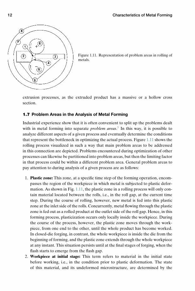
Figure 1.11. Representation of problem areas in rolling ofmetals.
extrusion processes, as the extruded product has a massive or a hollow crosssection.
1.7 Problem Areas in the Analysis of Metal Forming
Industrial experience show that it is often convenient to split up the problems dealtwith in metal forming into separate problem areas.5 In this way, it is possible toanalyze different aspects of a given process and eventually determine the conditionsthat represent the bottleneck in optimizing the actual process. Figure 1.11 shows therolling process visualized in such a way that main problem areas to be addressedin this connection are depicted. Problems encountered during optimization of otherprocesses can likewise be partitioned into problem areas, but then the limiting factorin that process could be within a different problem area. General problem areas topay attention to during analysis of a given process are as follows:
1. Plastic zone: This zone, at a specific time step of the forming operation, encom-passes the region of the workpiece in which metal is subjected to plastic defor-mation. As shown in Fig. 1.11, the plastic zone in a rolling process will only con-tain material located between the rolls, i.e., in the roll gap, at the current timestep. During the course of rolling, however, new metal is fed into this plasticzone at the inlet side of the rolls. Concurrently, metal flowing through the plasticzone is fed out as a rolled product at the outlet side of the roll gap. Hence, in thisforming process, plasticization occurs only locally inside the workpiece. Duringthe course of the process, however, the plastic zone moves through the work-piece, from one end to the other, until the whole product has become worked.In closed-die forging, in contrast, the whole workpiece is inside the die from thebeginning of forming, and the plastic zone extends through the whole workpieceat any instant. This situation persists until at the final stages of forging, when theflash starts to emerge from the flash gap.
2. Workpiece at initial stage: This term refers to material in the initial statebefore working, i.e., in the condition prior to plastic deformation. The stateof this material, and its undeformed microstructure, are determined by the
1.7 Problem Areas in the Analysis of Metal Forming 13
thermomechanical treatment it has been given previously; whether it has beenworked, or annealed; and whether it is cold, warm, or hot.
3. Workpiece at final stage, i.e., the final worked product: The final product con-sists of the actual material after forming, with its mechanical properties, whichmay have been significantly altered by plastic working of the material during theforming process. The result is either a wrought product to be processed furtherbefore use, or a finished product ready for final use after forming.
4. Interface between workpiece and die: When the die is pressed into the work-piece, contact is established between the surfaces of the two bodies. Therecan be direct contact between the workpiece and the die, but indirect contactthrough their oxide films is more common. Contact may eventually be estab-lished through lubricant films that partially or completely separate the two bod-ies. The characteristic layer(s) separating the bulk material of the two bodiesfrom each other are commonly termed an interface. The surfaces that establishcontact during the forming operation will have their typical initial topography,including surface roughness and oxide films that partially or completely coverthe surfaces.
The nature and the mechanical behavior of the contact interface betweendie and workpiece can be crucial for the stability of the metal forming process.If the lubricant film at the interface suffers breakdown during the forming oper-ation, lumps of workpiece metal can locally pressure-weld onto the die. If thishappens, the next component that is formed will be one with wrong geometry orof bad surface quality, depending on how much metal transfer there has been.With metal transfer to the die the process must be interrupted, so that the diescan be cleaned, before forming can be resumed.
5. Dies: As mentioned previously, the cost of making dies is usually rather high inmetal forming. Therefore, to obtain sound process economy in metal forming,the dies must be made with good design and from a material that ensures acertain minimum die life. The dies should be able to shape many componentswithout being subjected to unacceptable wear or to failure.
6. Surface layer of the workpiece and product: In metal forming, the surface prop-erties of the initial workpiece are important for various reasons. One reasonis that it may influence the effectiveness of the lubricant that is used. Anotherimportant aspect is that, if the surface film is abrasive, it may cause excessive diewear. Of special importance is of course the surface quality, or surface finish, ofthe resulting product. If the surface contains scars, or appears with a matte ordull finish, the resulting product may not satisfy the requirements of the cus-tomer and, in that case, has to be discarded.
7. Forming machine: For metal forming, the machines applied are most com-monly complex and expensive to buy. It is obvious that the forming machinesshould be made so they are well suited for their specific use, so productionproceeds smoothly, without unintended interruptions. If these requirementsare fulfilled, high productivity can be maintained in metal forming, with soundprocess economy.
14 Characteristics of Metal Forming
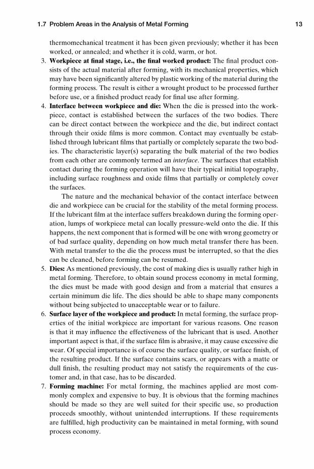
Figure 1.12. Important process parameters in metal forming.
8. Company: To obtain a good economical result as a whole, it is obvious thatyour company must be well organized and efficient, so that production is basedon sound economic premises.
1.8 Important Process Parameters in Metal Forming
As discussed in the preceding section, it is important for the economics of any metalforming process that forming be done in the best possible way. To create conditionsnear to the optimum, one should preferably, in each actual process, know how theforming conditions, i.e., the process parameters, influence the results of the produc-tion process. This topic will be dealt with in more detail in later chapters of the book.As an introduction, some of the most important of the general process parametersin metal forming are mentioned here; see Fig. 1.12. With respect to the workpiece,it is important that it has sufficient formability to allow the intended amount of plas-tic deformations that is required without the material developing cracks or otherdefects.
Inside the plastic zone of the workpiece it is important to be able to measureand control such quantities as the strain ε, the strain rate ε, the flow stress σ , and thetemperature T that the material is exposed to. In the interface between the work-piece and the die, the important local parameters are the temperature T, the contactpressure p, and the shear stress τ due to friction forces transferred from the work-piece to the die.
These parameters are often influenced by the quality of the lubricant applied.The required forming load is influenced by the mentioned parameters and mustnot exceed the force provided by the actual forming machine. If it does, formingcannot be accomplished. As mentioned before, the mechanical properties of thefinal product in metal forming are also influenced by the deformation conditionsduring the forming operation.
Problems 15
If the product is to be applied in the as-formed condition, without later heattreatment, it is essential that the resulting mechanical properties should meet therequirements specified by the user of the product.
Problems
1.1. State the main assumptions made in continuum mechanics about how the mate-rial is composed when considered on the micro scale. Does this agree with ourknowledge of the real microstructure of metallic materials?
1.2. Describe how particle-strengthened Al alloys are built up when considered onatomic level. How does this agree with the common assumptions made in continuummechanics?
1.3. Describe the most typical characteristics of metal forming as a manufacturingprocess.
1.4. What are the names of the two manufacturing processes most commonly usedinstead of metal forming? Specify the main advantages and disadvantages of theseclasses of processes in comparison with metal forming.
1.5 Specimens made from a soft-annealed plate consisting of the aluminum alloyAl99.5 are given the following treatments:
(i) Cold-rolled from 10 mm down to 1 mm final thickness.(ii) Cold-rolled from 10 mm down to 0.1 mm final thickness.
(iii) Treated as (ii) and then annealed at 150◦C.(iv) Treated as (ii) and then annealed at 350◦C.
What mechanical properties you would expect to achieve in the final metalafter these treatments?
1.6 A finite element method simulation model of cylinder compression with highfriction is available as a video clip at the homepage of the book. In the simulation,the flow-net option of the software was used to visualize how an initial grid patterninside the metal will deform during cylinder compression. Run the animation fromthis simulation and observe how the internal grid pattern changes as compressionproceeds. On basis of your observations, describe the following:
(i) The FEM-predicted change of the outer shape of the cylinder.(ii) The predicted deformational behavior of the grid pattern at the center
of the cylinder in comparison with the behavior at the periphery of thecylinder.
1.7. Make a sketch similar to Fig. 1.11, and indicate problem areas to be analyzed inmetal forming when indirect extrusion is used.
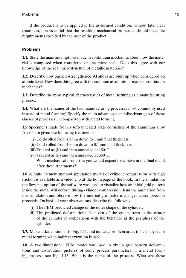
1.8. A two-dimensional FEM model was used to obtain grid pattern deforma-tions and distribution pictures of some process parameters in a metal form-ing process; see Fig. 1.13. What is the name of the process? What are these
16 Characteristics of Metal Forming
(a)
(b)
(c)
Step 10
z
X(R)Step 61
Punchhead
Container
Figure 1.13. Postprocessing results from 2D FEM-model of metal forming operation.

References 17
process parameters, and what kind of information can be obtained from the pic-tures?
NOTES
1. http://en.wikipedia.org/wiki/Continuum mechanics2. “MNC Handbok nr 12, Aluminium, Konstruktions- og Materiallara,” ed. 1, Dec. 1983
(in Swedish).3. Smidesteknik, Larobok, Smidesgruppen innom Sveriges mekanforbund, Stockholm,
1983, pp. 12–13 (in Swedish).4. DIN 8583, “Manufacturing Processes, Compressive Methods,” ed. 2003–09 (in German).5. Lange, K.: “A system for the investigation of metal forming processes,” Proc. 10th Int.
M.T.D.R. Conf., Univ. of Manchester, 1969, Pergamon Press, 1970.
REFERENCES
Dieter, G. E. “Mechanical Metallurgy,” McGraw-Hill, 1989.Kalpakjian, S., and Schmid, S. R. “Manufacturing Processes for Engineering Materials,” 5th
ed., Prentice-Hall, 2008.Lange, K. “Handbook of Metal Forming,” McGraw-Hill, 1985.Mielnik, E. M. “Metalworking Science and Engineering,” McGraw-Hill, 1991.

2 Important Metal Forming Processes
Although there are many different metal forming processes, in this chapter onlysome of the most important processes will be described. A more complete overviewof metal forming processes is given elsewhere.1,2 A classification system that is use-ful for those who are not experienced metal formers will also be described.
2.1 Classification System for Metal Forming Processes
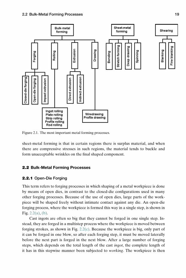
In Fig. 1.9, a sketch was shown in which the primary metal forming processes wereorganized among various common manufacturing methods. In Fig. 2.1, we haveexpanded the metal forming region downward, thus including the most significantmetal forming processes. As seen from this figure, the processes at the lowest levelof the diagram are commonly described by the name of the product created by thatparticular forming process.
Figure 2.1 also shows the important distinction between bulk-metal formingand sheet-metal forming. Bulk-metal forming is the shaping of bodies with con-centrated mass, i.e., where the dimensions in each of the three orthogonal direc-tions x, y, and z of the body are of similar size. Sheet-metal forming, on the otherhand, is the forming of bodies with initial large extensions in two directions andsmall extension in the third direction, such as in a piece of sheet metal or a steelplate.
As mentioned before, sheet-metal forming is quite different from bulk-metalforming. In sheet-metal forming, a relatively thin, wide sheet is formed against a die.In this case, it is impossible to keep the workpiece inside a configuration of closeddies. In sheet-metal forming, the material is therefore most commonly subjected totensile stresses, in contrast to bulk-metal forming, where compressive stresses dom-inate. Because of the presence of tensile stresses in sheet-metal forming, there arestrong limitations with regard to the degree of shaping of the workpiece that is pos-sible, without encountering problems related to material instability – for example,in terms of formation of a neck. During further forming, such a neck would tend togrow, and that would finally lead to rupture of the workpiece. Another problem in
18
2.2 Bulk-Metal Forming Processes 19
--
Figure 2.1. The most important metal forming processes.
sheet-metal forming is that in certain regions there is surplus material, and whenthere are compressive stresses in such regions, the material tends to buckle andform unacceptable wrinkles on the final shaped component.
2.2 Bulk-Metal Forming Processes
2.2.1 Open-Die Forging
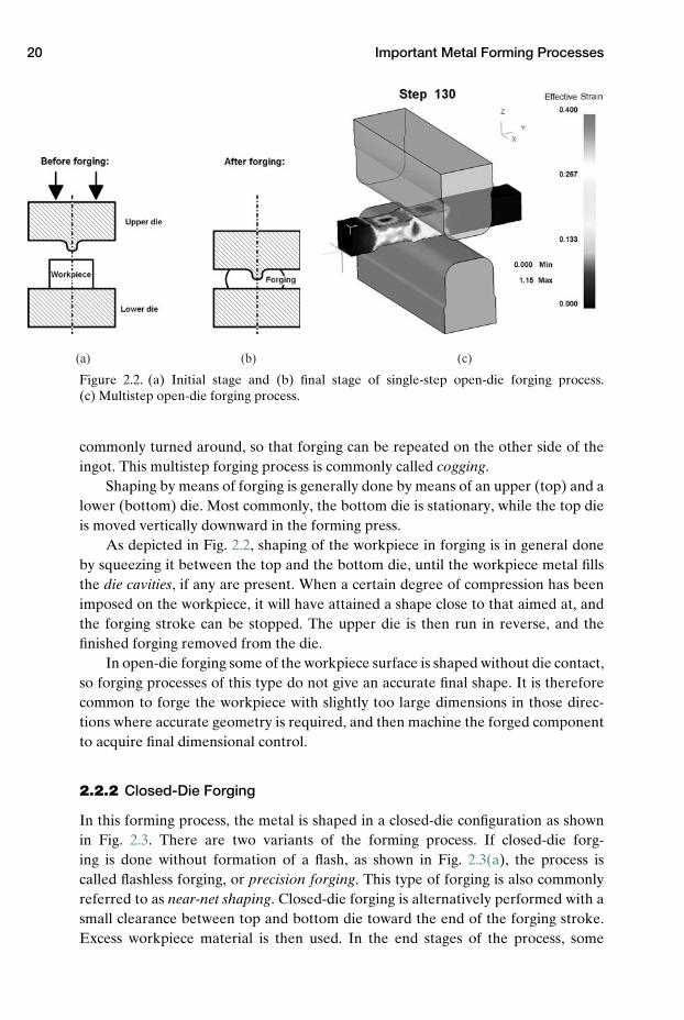
This term refers to forging processes in which shaping of a metal workpiece is doneby means of open dies, in contrast to the closed-die configurations used in manyother forging processes. Because of the use of open dies, large parts of the work-piece will be shaped freely without intimate contact against any die. An open-dieforging process, where the workpiece is formed this way in a single step, is shown inFig. 2.2(a), (b).
Cast ingots are often so big that they cannot be forged in one single step. In-stead, they are forged in a multistep process where the workpiece is moved betweenforging strokes, as shown in Fig. 2.2(c). Because the workpiece is big, only part ofit can be forged in one blow, so after each forging step, it must be moved laterallybefore the next part is forged in the next blow. After a large number of forgingsteps, which depends on the total length of the cast ingot, the complete length ofit has in this stepwise manner been subjected to working. The workpiece is then
20 Important Metal Forming Processes
(a) (b) (c)
Figure 2.2. (a) Initial stage and (b) final stage of single-step open-die forging process.(c) Multistep open-die forging process.
commonly turned around, so that forging can be repeated on the other side of theingot. This multistep forging process is commonly called cogging.
Shaping by means of forging is generally done by means of an upper (top) and alower (bottom) die. Most commonly, the bottom die is stationary, while the top dieis moved vertically downward in the forming press.
As depicted in Fig. 2.2, shaping of the workpiece in forging is in general doneby squeezing it between the top and the bottom die, until the workpiece metal fillsthe die cavities, if any are present. When a certain degree of compression has beenimposed on the workpiece, it will have attained a shape close to that aimed at, andthe forging stroke can be stopped. The upper die is then run in reverse, and thefinished forging removed from the die.
In open-die forging some of the workpiece surface is shaped without die contact,so forging processes of this type do not give an accurate final shape. It is thereforecommon to forge the workpiece with slightly too large dimensions in those direc-tions where accurate geometry is required, and then machine the forged componentto acquire final dimensional control.
2.2.2 Closed-Die Forging
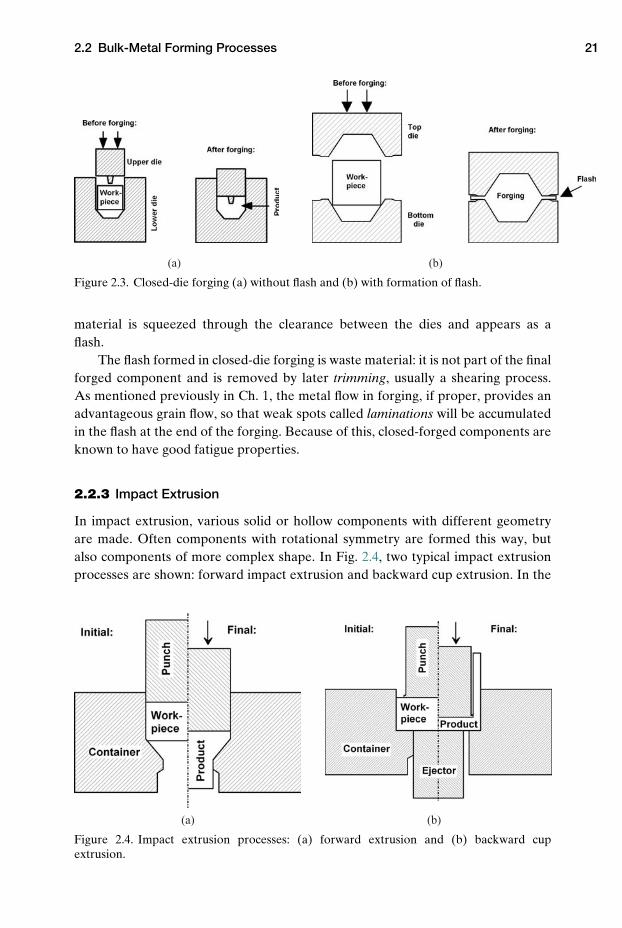
In this forming process, the metal is shaped in a closed-die configuration as shownin Fig. 2.3. There are two variants of the forming process. If closed-die forg-ing is done without formation of a flash, as shown in Fig. 2.3(a), the process iscalled flashless forging, or precision forging. This type of forging is also commonlyreferred to as near-net shaping. Closed-die forging is alternatively performed with asmall clearance between top and bottom die toward the end of the forging stroke.Excess workpiece material is then used. In the end stages of the process, some
2.2 Bulk-Metal Forming Processes 21
(a) (b)
Figure 2.3. Closed-die forging (a) without flash and (b) with formation of flash.
material is squeezed through the clearance between the dies and appears as aflash.
The flash formed in closed-die forging is waste material: it is not part of the finalforged component and is removed by later trimming, usually a shearing process.As mentioned previously in Ch. 1, the metal flow in forging, if proper, provides anadvantageous grain flow, so that weak spots called laminations will be accumulatedin the flash at the end of the forging. Because of this, closed-forged components areknown to have good fatigue properties.
2.2.3 Impact Extrusion
In impact extrusion, various solid or hollow components with different geometryare made. Often components with rotational symmetry are formed this way, butalso components of more complex shape. In Fig. 2.4, two typical impact extrusionprocesses are shown: forward impact extrusion and backward cup extrusion. In the
(a) (b)
Figure 2.4. Impact extrusion processes: (a) forward extrusion and (b) backward cupextrusion.

22 Important Metal Forming Processes
(b)(a)
1 2 3 4 5 6 7
Figure 2.5. Rolling: (a) flat rolling and (b) rolling schedule in section rolling.
forward extrusion process [see Fig. 2.4(a)], the workpiece moves in the same direc-tion as the punch, whereas in the backward process [see Fig. 2.4(b)], the movementof the workpiece material is opposite to that of the punch.
2.2.4 Rolling
In rolling processes, the workpiece, for instance, a plate, is rolled between two rolls[see Fig. 2.5(a)], so that the plate is compressed in its thickness direction. As a con-sequence of this, the plate thickness is reduced. Because of the constancy of volume,the plate must, however, expand in the other directions: in the length direction andalso to some extent in the width direction. Rolling can be divided into two types,depending on whether a flat product is rolled, or a product of more complex cross-sectional shape is worked. When flat products are rolled, the process is commonlytermed flat rolling. When long profiles of complex cross-sectional shape are pro-duced, the process is called profile or section rolling. Profiles are long beams of var-ious cross-sectional shapes. Common rolled profiles are for instance beams with I-,H-, or L-shaped cross section.
One or two decades ago, steels were commonly cast in big ingots with square,or close to square, cross section. They were first rolled down in a roughening rollingmill to semifinished products of smaller cross section. In this way, semifinished stocklike slabs, blooms, and billets were processed. A slab had a large rectangular crosssection and was subsequently rolled down in a plate or a strip rolling mill to aplate or strip. A bloom had a large, and a billet had a smaller, square cross sec-tion. Both were processed further in shape rolling mills: the blooms were rolledinto large sections, and the billets were rolled into smaller sections or into rod orwire.
Today, new casting processes have been developed, so this large productionequipment has to a large extent been replaced by smaller, cheaper machines. Todayslabs, blooms, and billets are most commonly made by casting in continuous castingfacilities. Afterwards the slabs are rolled down to plate or strip. Plates are, as thename indicates, flat products with large length and width, whereas strips have largelength but smaller width. Strip material is often coiled after rolling, because this
2.2 Bulk-Metal Forming Processes 23
(a) (b)
Container
Profile
Die
Billet
Ram
Pro
file
Closing pad
Die
Billet
Ram
Container
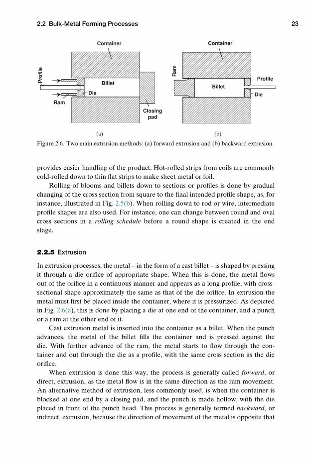
Figure 2.6. Two main extrusion methods: (a) forward extrusion and (b) backward extrusion.
provides easier handling of the product. Hot-rolled strips from coils are commonlycold-rolled down to thin flat strips to make sheet metal or foil.
Rolling of blooms and billets down to sections or profiles is done by gradualchanging of the cross section from square to the final intended profile shape, as, forinstance, illustrated in Fig. 2.5(b). When rolling down to rod or wire, intermediateprofile shapes are also used. For instance, one can change between round and ovalcross sections in a rolling schedule before a round shape is created in the endstage.
2.2.5 Extrusion
In extrusion processes, the metal – in the form of a cast billet – is shaped by pressingit through a die orifice of appropriate shape. When this is done, the metal flowsout of the orifice in a continuous manner and appears as a long profile, with cross-sectional shape approximately the same as that of the die orifice. In extrusion themetal must first be placed inside the container, where it is pressurized. As depictedin Fig. 2.6(a), this is done by placing a die at one end of the container, and a punchor a ram at the other end of it.
Cast extrusion metal is inserted into the container as a billet. When the punchadvances, the metal of the billet fills the container and is pressed against thedie. With further advance of the ram, the metal starts to flow through the con-tainer and out through the die as a profile, with the same cross section as the dieorifice.
When extrusion is done this way, the process is generally called forward, ordirect, extrusion, as the metal flow is in the same direction as the ram movement.An alternative method of extrusion, less commonly used, is when the container isblocked at one end by a closing pad, and the punch is made hollow, with the dieplaced in front of the punch head. This process is generally termed backward, orindirect, extrusion, because the direction of movement of the metal is opposite that
24 Important Metal Forming Processes
of the ram movement. The two methods of extrusion, direct and indirect, are shownschematically in Fig. 2.6.
Backward extrusion has certain advantages over forward extrusion, in that itdoes not require pressing the billet through the container. Because of this, therequired extrusion force is lower, and in addition, there is better dimensionalstability of the extruded profile – the extrudate. A third advantage is that the defor-mation of the metal flowing out through the die opening is more constant along thelength of the profile than in forward extrusion, for there is almost zero predefor-mation of the billet in its back portion. In forward extrusion, these predeformationsare bigger, especially the deformations of the peripheral layers of the billet, whichis forced to slide along the container wall with the advance of the ram.
Forward extrusion, however, is the most commonly used extrusion process,because the use of backward extrusion is considerably limited in two ways. Oneis that the extruded profile must be taken out from the press through the ram itself.Because of this, one must use a hollow ram. This imposes considerable practicaldifficulties, especially when multihole dies are used to extrude many profiles con-currently, or in the extrusion of profiles with large prescribed circumference. Thechallenge then is to make a ram design sufficiently strong to take the large extru-sion loads, because the ram must be hollow and the extrusions must be taken outthrough its hollow stem. Another limitation arises from the nature of metal flow inthe backward extrusion process. It is a fact that the peripheral layers of the billetin backward extrusion tend to flow much more easily through the die orifice thanin the forward process.
Billets are commonly produced in continuous casting processes, where logs oflarge length are made. Afterwards the logs are sheared into appropriate pieces – thebillets. Because of the casting process, a billet has a peripheral cast surface layer, ofless metallurgical quality than the core. For this reason, better surface quality isnormally obtained in forward extrusion than in backward extrusion.
To obtain sufficient surface quality in backward extrusion, it may be necessaryeither to machine away the inferior surface layers of the billet before extrusion orto leave a shell of billet material in the container during extrusion. This is done byusing a small clearance between the die and the container wall. Both variants ofthe backward extrusion technique involve additional operations in comparison withdirect extrusion and hence also additional costs.
Aluminum and its alloys have low flow stress at temperatures in the range 400–500◦C. Because of this, they can be hot-extruded into profiles with complex cross-sectional shape. In extrusion of copper or brass, there is less freedom regardingextrudable shapes, because the extrusion temperature required is as high as 700–1000◦C. Even at these high temperatures, the flow stress of these metals is high.Because of this, the combined thermal and mechanical loads on the tooling arehigh. Therefore, if complex shapes are extruded on the same principles as in alu-minum extrusion, the die life becomes too short to yield acceptable process econ-omy. Hence, for copper and brasses, there are strong limitations as regards thecomplexity of the shape of the profiles that can be extruded with sound process
2.2 Bulk-Metal Forming Processes 25
Billet
Port
BridgeNo. 1
BridgeNo. 2
Extrusionseam weld
BridgeNo. 3
Weldingchamber Tube
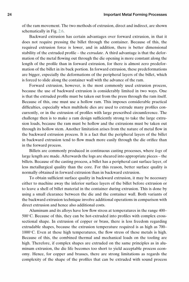
Figure 2.7. Material flow in hollow for-ward extrusion.
economy. For steels, the conditions in extrusion are even worse; extrusion tempera-tures of 1000–1200◦C are required. Continuous extrusion processes applied for steel,on the same principles as for aluminum, copper, and brass, are therefore rare. Con-ditions are so severe that it is difficult to find die materials that will survive for a suffi-ciently long time. For steel materials, however, a lubricated hot-extrusion techniquebased on use of glass lubrication, which melts down ahead of the die, has been devel-oped. With this technology, it is possible to extrude small sections with low shapecomplexity. Continuous hot extrusion of steel is, however, highly specialized and isnot so commonly used.
Because of the good hot extrudability of aluminum and its alloys, they can evenbe extruded into very complex hollow profiles,3 as for instance tubes, in a simi-lar way to extrusion of plastics. This is done using hollow extrusion dies of highcomplexity. The best way to understand how this is done is to look at the metalflow in the tube extrusion process. The metal flow in this process, in which a tubeis extruded by means of a porthole die with an inner mandrel and three bridges,or webs, is shown in the three-dimensional sketch in Fig. 2.7. Here only the metalof the billet, flowing through the die, and the resulting profile are shown; the com-plete steel dies, or tooling, which surround the metal, have been omitted to enableexamining the process.
As one can see from the sketch, the billet is split in three separate metalstreams when it is pushed against the bridges of the die, filling its three portholes.When the metal streams reach the bottom of the ports, they meet again in the weld-ing chamber, where they are joined together into one metal stream by pressurewelding. At this instant, the metal becomes shaped into a tube. The inner hole ofthe tube is formed against the mandrel placed in the middle of the die, the man-drel being carried by the bridges. The circumferential outer part of the die shapesthe outside of the tube, as the metal flows through the gap between the mandreland the outer part of the die. Since the metal flow is characterized by splitting themetal stream into separate streams, later to be joined again, the process is based
26 Important Metal Forming Processes
(b)(a)
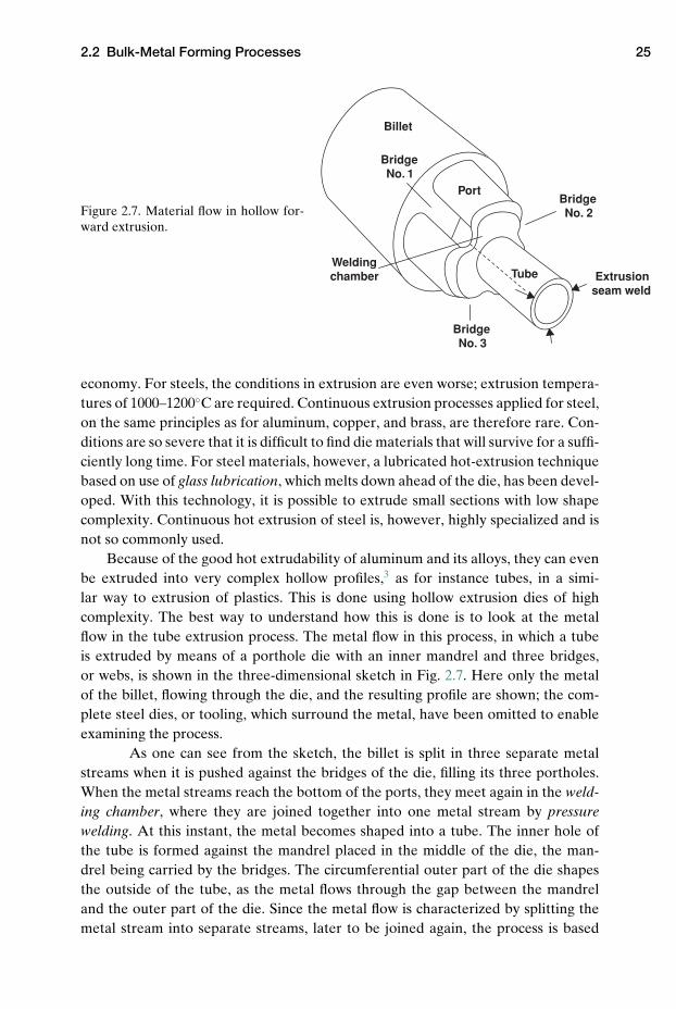
Figure 2.8. (a) Wiredrawing and (b) deep drawing of sheet metal.
on pressure welding, or extrusion welding, as it is generally named. At the rear endof each bridge, two metal streams join by welding, and an extrusion weld is formed.The weld flows out of the die and appear as an extrusion seam weld in the resultinghollow profile. Hollow profiles made this way have the same number of longitu-dinal seam welds distributed over the cross section as the number of bridges usedin the die.
2.2.6 Wiredrawing
As shown in Fig. 2.8(a), a thin rod or wire can be manufactured from a thickerinitial rod or wire by pulling it through a die shaped with an inner conical die chan-nel. To maintain stable wire dimension out of the die, the converging channel mustbe followed by a parallel bearing. Because of constancy of volume during form-ing, the length of the wire will increase correspondingly when the cross section ofthe wire is reduced. To be able to draw the wire through the die, a pulling forceis required behind the die. Wires are drawn in long continuous lengths – mostcommonly from a coil of thicker wire, which originally was made in a hot-rollingprocess.
To avoid stopping the continuous production process, the wire from one coil isjoined to the wire from the next, by pressure- or fusion-welding the ends of the twocoils together. In this way, the process can be run continuously for a long time, ifwire breaks do not occur.
To pull the wire through the die, it is required to use a drawing wheel, also calleda capstan, at the back of the drawing die, to provide pulling force to the wire. Whenthe wire has been reduced in a reduction step by one die, it is fed in a continuousmovement by the capstan to the second die. This die has smaller diameter than thefirst die, and a second capstan is required to pull the wire. By placing as many as 20draw cells – consisting of a die and a capstan – in sequence, wire of small diametercan be produced, in a continuous process, from initially thick wire. In drawing, itis common to use a constant reduction in each drawing step, which is usually kept
2.3 Sheet-Metal Forming Processes 27
below 20%. After the end of the last drawing unit, there is usually a rotating spoolerin the wiredrawing machine, which accumulates the wire on a spool.
Rod and profiles can also be processed by drawing through dies. If they havea large cross section, or if there are tight dimensional requirements on the finishedproduct, they are kept in straight lengths before and after drawing. Because of thestiffness of the die, drawing gives good dimensional stability to the finished prod-uct, i.e., there is less dimensional variation along the length of it than if the sameproduct is made by rolling or extrusion. Drawing is therefore used as a calibrationprocess in cases where final product dimensions are to be kept within narrowtolerances.
As previously shown in Fig. 1.7, cold deformation will increase the strength andthe hardness of metals. Because of this, cold drawing is used to fabricate hard vari-ants of initially soft alloys, so that the metal is strengthened by the drawing process,and a product with improved mechanical properties (increased yield strength andtensile strength) is obtained.
If a metal, or an alloy, is to be drawn through many successive dies, it is requiredto soft-anneal it at an intermediate drawing stage, because cold working increasesthe hardness of the material and reduces its ductility. In an intermediate soft-annealing process, the initial high ductility of the wire can be restored. After this,drawing can be continued further, without the risk of wire breaks or excessive diewear. By repeated sequences of drawing followed by soft annealing, wires finer thana human hair can be manufactured at a reasonable price.
2.3 Sheet-Metal Forming Processes
2.3.1 Deep Drawing
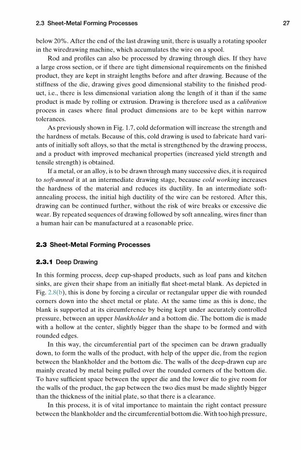
In this forming process, deep cup-shaped products, such as loaf pans and kitchensinks, are given their shape from an initially flat sheet-metal blank. As depicted inFig. 2.8(b), this is done by forcing a circular or rectangular upper die with roundedcorners down into the sheet metal or plate. At the same time as this is done, theblank is supported at its circumference by being kept under accurately controlledpressure, between an upper blankholder and a bottom die. The bottom die is madewith a hollow at the center, slightly bigger than the shape to be formed and withrounded edges.
In this way, the circumferential part of the specimen can be drawn graduallydown, to form the walls of the product, with help of the upper die, from the regionbetween the blankholder and the bottom die. The walls of the deep-drawn cup aremainly created by metal being pulled over the rounded corners of the bottom die.To have sufficient space between the upper die and the lower die to give room forthe walls of the product, the gap between the two dies must be made slightly biggerthan the thickness of the initial plate, so that there is a clearance.
In this process, it is of vital importance to maintain the right contact pressurebetween the blankholder and the circumferential bottom die. With too high pressure,
28 Important Metal Forming Processes
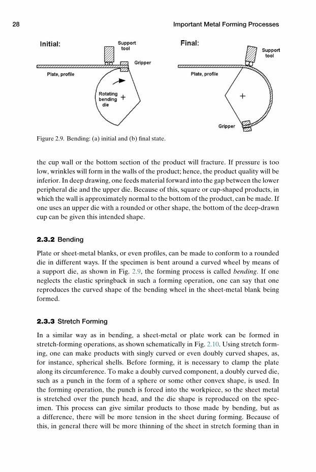
Figure 2.9. Bending: (a) initial and (b) final state.
the cup wall or the bottom section of the product will fracture. If pressure is toolow, wrinkles will form in the walls of the product; hence, the product quality will beinferior. In deep drawing, one feeds material forward into the gap between the lowerperipheral die and the upper die. Because of this, square or cup-shaped products, inwhich the wall is approximately normal to the bottom of the product, can be made. Ifone uses an upper die with a rounded or other shape, the bottom of the deep-drawncup can be given this intended shape.
2.3.2 Bending
Plate or sheet-metal blanks, or even profiles, can be made to conform to a roundeddie in different ways. If the specimen is bent around a curved wheel by means ofa support die, as shown in Fig. 2.9, the forming process is called bending. If oneneglects the elastic springback in such a forming operation, one can say that onereproduces the curved shape of the bending wheel in the sheet-metal blank beingformed.
2.3.3 Stretch Forming
In a similar way as in bending, a sheet-metal or plate work can be formed instretch-forming operations, as shown schematically in Fig. 2.10. Using stretch form-ing, one can make products with singly curved or even doubly curved shapes, as,for instance, spherical shells. Before forming, it is necessary to clamp the platealong its circumference. To make a doubly curved component, a doubly curved die,such as a punch in the form of a sphere or some other convex shape, is used. Inthe forming operation, the punch is forced into the workpiece, so the sheet metalis stretched over the punch head, and the die shape is reproduced on the spec-imen. This process can give similar products to those made by bending, but asa difference, there will be more tension in the sheet during forming. Because ofthis, in general there will be more thinning of the sheet in stretch forming than in
2.3 Sheet-Metal Forming Processes 29
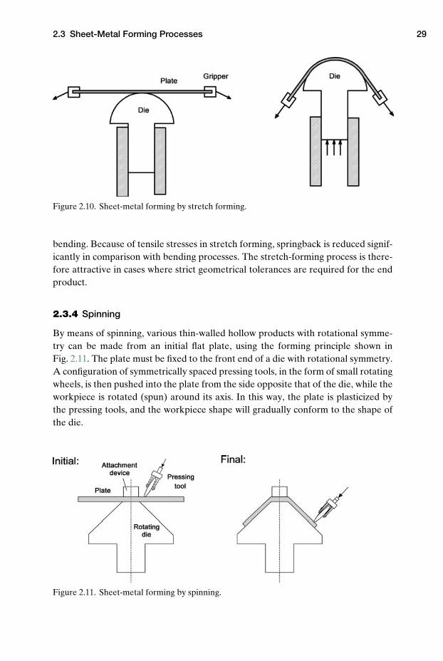
Figure 2.10. Sheet-metal forming by stretch forming.
bending. Because of tensile stresses in stretch forming, springback is reduced signif-icantly in comparison with bending processes. The stretch-forming process is there-fore attractive in cases where strict geometrical tolerances are required for the endproduct.
2.3.4 Spinning
By means of spinning, various thin-walled hollow products with rotational symme-try can be made from an initial flat plate, using the forming principle shown inFig. 2.11. The plate must be fixed to the front end of a die with rotational symmetry.A configuration of symmetrically spaced pressing tools, in the form of small rotatingwheels, is then pushed into the plate from the side opposite that of the die, while theworkpiece is rotated (spun) around its axis. In this way, the plate is plasticized bythe pressing tools, and the workpiece shape will gradually conform to the shape ofthe die.
Figure 2.11. Sheet-metal forming by spinning.
30 Important Metal Forming Processes
Final:Initial:
-
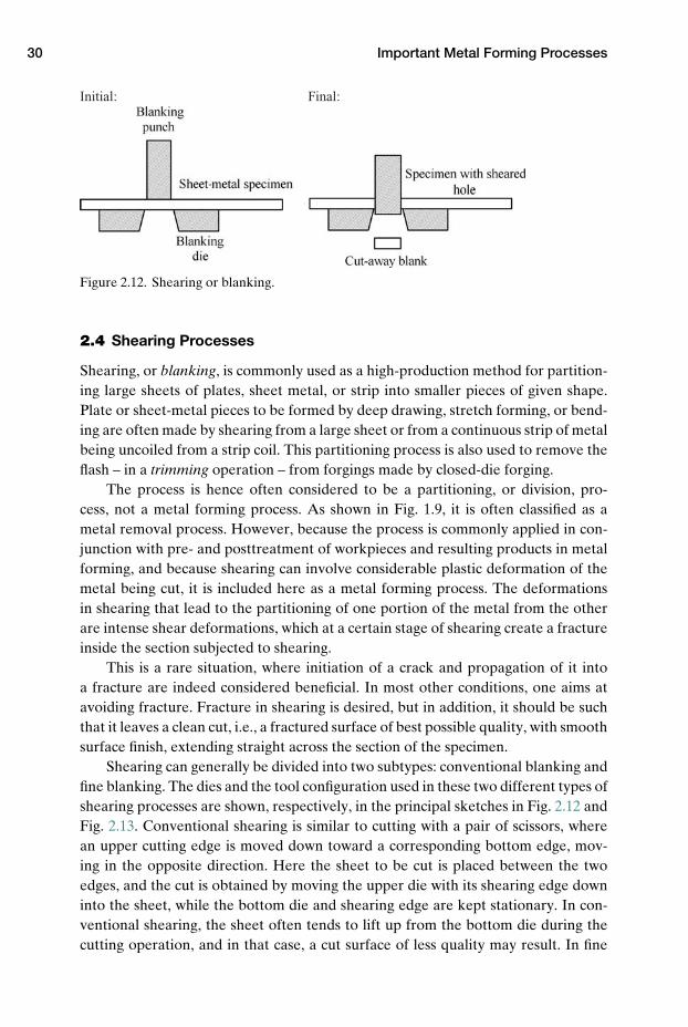
Figure 2.12. Shearing or blanking.
2.4 Shearing Processes
Shearing, or blanking, is commonly used as a high-production method for partition-ing large sheets of plates, sheet metal, or strip into smaller pieces of given shape.Plate or sheet-metal pieces to be formed by deep drawing, stretch forming, or bend-ing are often made by shearing from a large sheet or from a continuous strip of metalbeing uncoiled from a strip coil. This partitioning process is also used to remove theflash – in a trimming operation – from forgings made by closed-die forging.
The process is hence often considered to be a partitioning, or division, pro-cess, not a metal forming process. As shown in Fig. 1.9, it is often classified as ametal removal process. However, because the process is commonly applied in con-junction with pre- and posttreatment of workpieces and resulting products in metalforming, and because shearing can involve considerable plastic deformation of themetal being cut, it is included here as a metal forming process. The deformationsin shearing that lead to the partitioning of one portion of the metal from the otherare intense shear deformations, which at a certain stage of shearing create a fractureinside the section subjected to shearing.
This is a rare situation, where initiation of a crack and propagation of it intoa fracture are indeed considered beneficial. In most other conditions, one aims atavoiding fracture. Fracture in shearing is desired, but in addition, it should be suchthat it leaves a clean cut, i.e., a fractured surface of best possible quality, with smoothsurface finish, extending straight across the section of the specimen.
Shearing can generally be divided into two subtypes: conventional blanking andfine blanking. The dies and the tool configuration used in these two different types ofshearing processes are shown, respectively, in the principal sketches in Fig. 2.12 andFig. 2.13. Conventional shearing is similar to cutting with a pair of scissors, wherean upper cutting edge is moved down toward a corresponding bottom edge, mov-ing in the opposite direction. Here the sheet to be cut is placed between the twoedges, and the cut is obtained by moving the upper die with its shearing edge downinto the sheet, while the bottom die and shearing edge are kept stationary. In con-ventional shearing, the sheet often tends to lift up from the bottom die during thecutting operation, and in that case, a cut surface of less quality may result. In fine
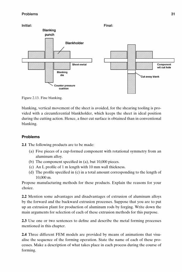
Problems 31
Final:Initial:
Figure 2.13. Fine blanking.
blanking, vertical movement of the sheet is avoided, for the shearing tooling is pro-vided with a circumferential blankholder, which keeps the sheet in ideal positionduring the cutting action. Hence, a finer cut surface is obtained than in conventionalblanking.
Problems
2.1 The following products are to be made:
(a) Five pieces of a cup-formed component with rotational symmetry from analuminum alloy.
(b) The component specified in (a), but 10,000 pieces.(c) An L profile of 1 m length with 10 mm wall thickness.(d) The profile specified in (c) in a total amount corresponding to the length of
10,000 m.Propose manufacturing methods for these products. Explain the reasons for yourchoice.
2.2 Mention some advantages and disadvantages of extrusion of aluminum alloysby the forward and the backward extrusion processes. Suppose that you are to putup an extrusion plant for production of aluminum rods by forging. Write down themain arguments for selection of each of these extrusion methods for this purpose.
2.3 Use one or two sentences to define and describe the metal forming processesmentioned in this chapter.
2.4 Three different FEM models are provided by means of animations that visu-alise the sequence of the forming operation. State the name of each of these pro-cesses. Make a description of what takes place in each process during the course offorming.
32 Important Metal Forming Processes
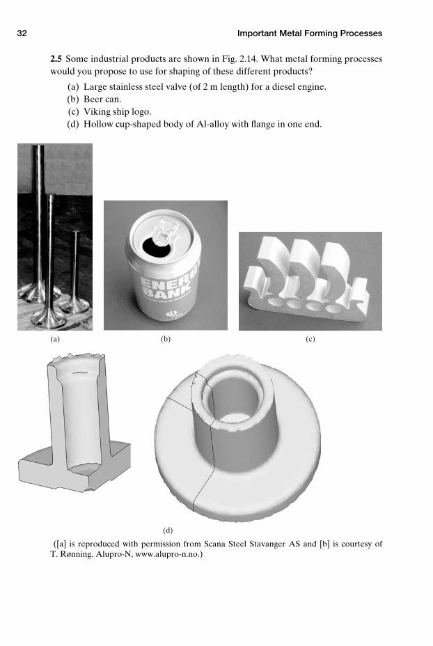
2.5 Some industrial products are shown in Fig. 2.14. What metal forming processeswould you propose to use for shaping of these different products?
(a) Large stainless steel valve (of 2 m length) for a diesel engine.(b) Beer can.(c) Viking ship logo.(d) Hollow cup-shaped body of Al-alloy with flange in one end.
(a) (b) (c)
(d)
([a] is reproduced with permission from Scana Steel Stavanger AS and [b] is courtesy ofT. Rønning, Alupro-N, www.alupro-n.no.)

References 33
NOTES
1. Altan, T., Oh, S.-I., and Gegel, H. L.: “Metal Forming, Fundamentals and Applications,”ASM, 1983, pp. 8–36.
2. Kalpakjian, S., and Schmid, S. R.: “Manufacturing Processes for Engineering Materials,”5th ed., Prentice-Hall, 2008.
3. Valberg, H.: “Extrusion welding in aluminium extrusion,” Int. J. Materials and ProductTechnology, Vol. 17, No. 7, 2002, pp. 497–556.
REFERENCES
“ASM Handbook, Vol. 14A, Metalworking: Bulk Forming,” ASM Int., 2005.“ASM Handbook, Vol. 14B: Metalworking: Sheet Forming,” ASM Int., 2006.Dieter, G. E.: “Mechanical Metallurgy,” McGraw-Hill, 1989.Lange, K.: “Handbook of Metal Forming,” McGraw-Hill, 1985.Mielnik, E. M.: “Metalworking Science and Engineering,” McGraw-Hill, 1991.

3 FEA of Metal Forming
Finite element analysis (FEA) has been developed during the last decades as a veryuseful tool for analysis of metal forming processes. Progress in development ofcheap and efficient computer technology, and the implementation of the finite ele-ment method (FEM) into user-friendly, window-based programs, has brought thistechnology forward. One can state that this development has more or less revolu-tionized the art of metal forming analysis.
In this chapter, it is demonstrated how 3D FEA can be applied for the analysisof a particular metal forming operation, namely, plane strain compression. To showhow well such analysis describes the actual conditions in metal forming, it is used tomodel and to reproduce a series of experiments conducted on an aluminum alloy inthe laboratory. In the experiments, an advanced grid pattern technique was used tocharacterize the real metal flow occurring in this deformation process.
3.1 The Plane Strain Compression Test
The plane strain compression1 test is conducted as either a cold- or a hot-formingtest. Although thermal effects are generally negligible in cold forming, they areimportant in hot forming. So to gain good accuracy, thermal effects must be includedin hot-forming models. The flow stress of the workpiece material is an importantparameter used in the FEM model. This parameter is very different in cold and inhot forming, as discussed in Ch. 8. Whereas flow stress is not significantly influencedby temperature in cold forming, in hot forming it depends strongly on temperature.
Schematic sketches of the test are shown in Fig. 3.1. Here (a) shows the ini-tial stage of the test in 3D view, and (b) and (c) show a longitudinal midsec-tion cut through the test, before and after compression, respectively. In the test,a rectangular strip, block, or slab is compressed in its midregion by two parallelplatens. The ends of the specimen remain unchanged, as they reside outside thecompression gap. The transverse plane in the middle of the specimen remains inthe same location during the compression stroke and is therefore called the neu-tral plane. Metal on both sides of this plane flows laterally away from the neutralplane. If initially far enough away from this plane, the material will flow out of the
34
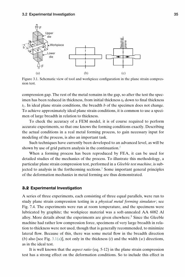
3.2 Experimental Investigation 35
F
F
Upper die
Workpiece
Lower die
b z xy
wt N
eutr
alpl
ane
(a) (b) (c)
Figure 3.1. Schematic view of tool and workpiece configuration in the plane strain compres-sion test.
compression gap. The rest of the metal remains in the gap, so after the test the spec-imen has been reduced in thickness, from initial thickness t0 down to final thicknesst1. In ideal plane strain conditions, the breadth b of the specimen does not change.To achieve approximately ideal plane strain conditions, it is common to use a speci-men of large breadth in relation to thickness.
To check the accuracy of a FEM model, it is of course required to performaccurate experiments, so that one knows the forming conditions exactly. Describingthe actual conditions in a real metal forming process, to gain necessary input formodeling of the process, is also an important task.
Such techniques have currently been developed to an advanced level, as will beshown by use of grid pattern analysis in the continuation.2
When a forming process has been reproduced by FEA, it can be used fordetailed studies of the mechanics of the process. To illustrate this methodology, aparticular plane strain compression test, performed in a Gleeble test machine, is sub-jected to analysis in the forthcoming sections.3 Some important general principlesof the deformation mechanics in metal forming are thus demonstrated.
3.2 Experimental Investigation
A series of three experiments, each consisting of three equal parallels, were run tostudy plane strain compression testing in a physical metal forming simulator ; seeFig. 7.4. The experiments were run at room temperature, and the specimens werelubricated by graphite; the workpiece material was a soft-annealed AA 6082 Alalloy. More details about the experiments are given elsewhere.3 Since the Gleeblemachine had rather low compression force, specimens of very large breadth in rela-tion to thickness were not used, though that is generally recommended, to minimizelateral flow. Because of this, there was some metal flow in the breadth direction(b) also [see Fig. 3.1(a)], not only in the thickness (t) and the width (w) directions,as in the ideal test.
It is well known that the aspect ratio (eq. 5-12) in the plane strain compressiontest has a strong effect on the deformation conditions. So to include this effect in
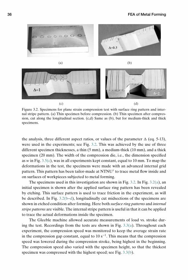
36 FEA of Metal Forming
(a)
(c) (d)
(b)
Figure 3.2. Specimens for plane strain compression test with surface ring pattern and inter-nal stripe pattern. (a) Thin specimen before compression. (b) Thin specimen after compres-sion, cut along the longitudinal section. (c,d) Same as (b), but for medium-thick and thickspecimens.
the analysis, three different aspect ratios, or values of the parameter � (eq. 5-13),were used in the experiments; see Fig. 3.2. This was achieved by the use of threedifferent specimen thicknesses, a thin (5 mm), a medium-thick (10 mm), and a thickspecimen (20 mm). The width of the compression die, i.e., the dimension specifiedas w in Fig. 3.5(c), was in all experiments kept constant, equal to 10 mm. To map thedeformations in the test, the specimens were made with an advanced internal gridpattern. This pattern has been tailor-made at NTNU4 to trace metal flow inside andon surfaces of workpieces subjected to metal forming.
The specimens used in this investigation are shown in Fig. 3.2. In Fig. 3.2(a), aninitial specimen is shown after the applied surface ring pattern has been revealedby etching. This surface pattern is used to trace friction in the experiment, as willbe described. In Fig. 3.2(b–d), longitudinally cut midsections of the specimens areshown in etched condition after forming. Here both surface ring patterns and internalstripe patterns are visible. The internal stripe pattern is useful in that it can be appliedto trace the actual deformations inside the specimen.
The Gleeble machine allowed accurate measurements of load vs. stroke dur-ing the test. Recordings from the tests are shown in Fig. 3.3(a). Throughout eachexperiment, the compression speed was monitored to keep the average strain ratein the compression gap constant, equal to 10 s−1. This means that the compressionspeed was lowered during the compression stroke, being highest in the beginning.The compression speed also varied with the specimen height, so that the thickestspecimen was compressed with the highest speed; see Fig. 3.3(b).
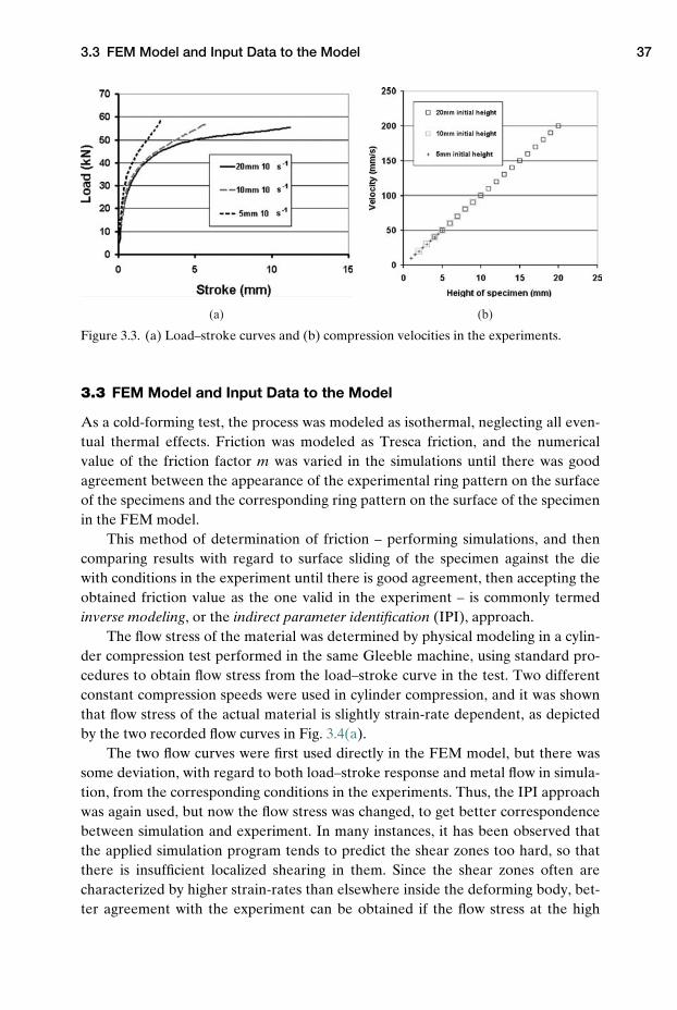
3.3 FEM Model and Input Data to the Model 37
(a) (b)
Figure 3.3. (a) Load–stroke curves and (b) compression velocities in the experiments.
3.3 FEM Model and Input Data to the Model
As a cold-forming test, the process was modeled as isothermal, neglecting all even-tual thermal effects. Friction was modeled as Tresca friction, and the numericalvalue of the friction factor m was varied in the simulations until there was goodagreement between the appearance of the experimental ring pattern on the surfaceof the specimens and the corresponding ring pattern on the surface of the specimenin the FEM model.
This method of determination of friction – performing simulations, and thencomparing results with regard to surface sliding of the specimen against the diewith conditions in the experiment until there is good agreement, then accepting theobtained friction value as the one valid in the experiment – is commonly termedinverse modeling, or the indirect parameter identification (IPI), approach.
The flow stress of the material was determined by physical modeling in a cylin-der compression test performed in the same Gleeble machine, using standard pro-cedures to obtain flow stress from the load–stroke curve in the test. Two differentconstant compression speeds were used in cylinder compression, and it was shownthat flow stress of the actual material is slightly strain-rate dependent, as depictedby the two recorded flow curves in Fig. 3.4(a).
The two flow curves were first used directly in the FEM model, but there wassome deviation, with regard to both load–stroke response and metal flow in simula-tion, from the corresponding conditions in the experiments. Thus, the IPI approachwas again used, but now the flow stress was changed, to get better correspondencebetween simulation and experiment. In many instances, it has been observed thatthe applied simulation program tends to predict the shear zones too hard, so thatthere is insufficient localized shearing in them. Since the shear zones often arecharacterized by higher strain-rates than elsewhere inside the deforming body, bet-ter agreement with the experiment can be obtained if the flow stress at the high
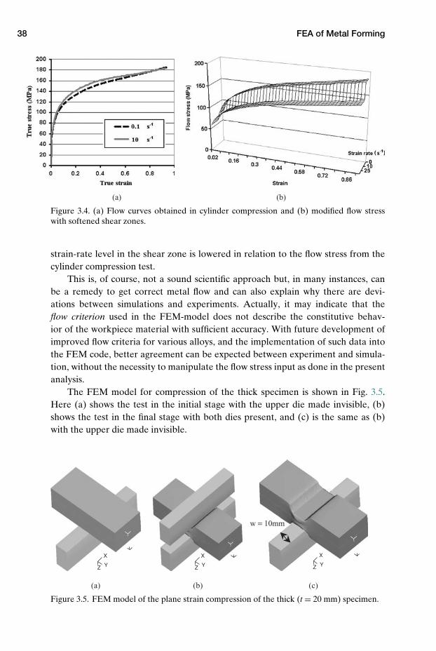
38 FEA of Metal Forming
(a) (b)
Figure 3.4. (a) Flow curves obtained in cylinder compression and (b) modified flow stresswith softened shear zones.
strain-rate level in the shear zone is lowered in relation to the flow stress from thecylinder compression test.
This is, of course, not a sound scientific approach but, in many instances, canbe a remedy to get correct metal flow and can also explain why there are devi-ations between simulations and experiments. Actually, it may indicate that theflow criterion used in the FEM-model does not describe the constitutive behav-ior of the workpiece material with sufficient accuracy. With future development ofimproved flow criteria for various alloys, and the implementation of such data intothe FEM code, better agreement can be expected between experiment and simula-tion, without the necessity to manipulate the flow stress input as done in the presentanalysis.
The FEM model for compression of the thick specimen is shown in Fig. 3.5.Here (a) shows the test in the initial stage with the upper die made invisible, (b)shows the test in the final stage with both dies present, and (c) is the same as (b)with the upper die made invisible.
(a) (b) (c)
w = 10mm
X
YZ
X
YZ
X
YZ
Figure 3.5. FEM model of the plane strain compression of the thick (t = 20 mm) specimen.
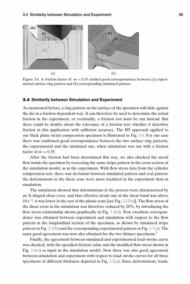
3.4 Similarity between Simulation and Experiment 39
(a) (b)
R2
R2R1
R1
Figure 3.6. A friction factor of m = 0.35 yielded good correspondence between (a) experi-mental surface ring pattern and (b) corresponding simulated pattern.
3.4 Similarity between Simulation and Experiment
As mentioned before, a ring pattern on the surface of the specimen will slide againstthe die in a friction-dependent way. It can therefore be used to determine the actualfriction in the experiment, or eventually, a friction test must be run instead. Butthere could be doubts about the relevance of a friction test: whether it describesfriction in this application with sufficient accuracy. The IPI approach applied toour thick plane strain compression specimen is illustrated in Fig. 3.6. For our casethere was confirmed good correspondence between the two surface ring patterns,the experimental and the simulated one, when simulation was run with a frictionfactor of m = 0.35.
After the friction had been determined this way, we also checked the metalflow inside the specimen by recreating the same stripe pattern in the cross section ofthe simulation model, as in the experiment. With flow stress data from the cylindercompression test, there was deviation between simulated pattern and real pattern:the deformations in the shear zone were more localized in the experiment than insimulation.
The simulation showed that deformations in the process were characterized byan X-shaped shear cross, and that effective strain rate in the shear band was above10 s−1; it was lower in the rest of the plastic zone [see Fig. 3.12(b)]. The flow stress ofthe shear cross in the simulation was therefore reduced by 20%, by introducing theflow stress relationship shown graphically in Fig. 3.4(b). Now excellent correspon-dence was obtained between experiment and simulation with respect to the flowpattern in the longitudinal section of the specimen, as shown by simulated stripepattern in Fig. 3.7(b) and the corresponding experimental pattern in Fig. 3.7(a). Thesame good agreement was now also obtained for the two thinner specimens.3
Finally, the agreement between simulated and experimented load–stroke curvewas checked, with the specified friction value and the modified flow stress shown inFig. 3.4(a) as input in the simulation model. Now there was also good agreementbetween simulation and experiment with respect to load–stroke curves for all threespecimens of different thickness depicted in Fig. 3.3(a). Since deformations, loads,
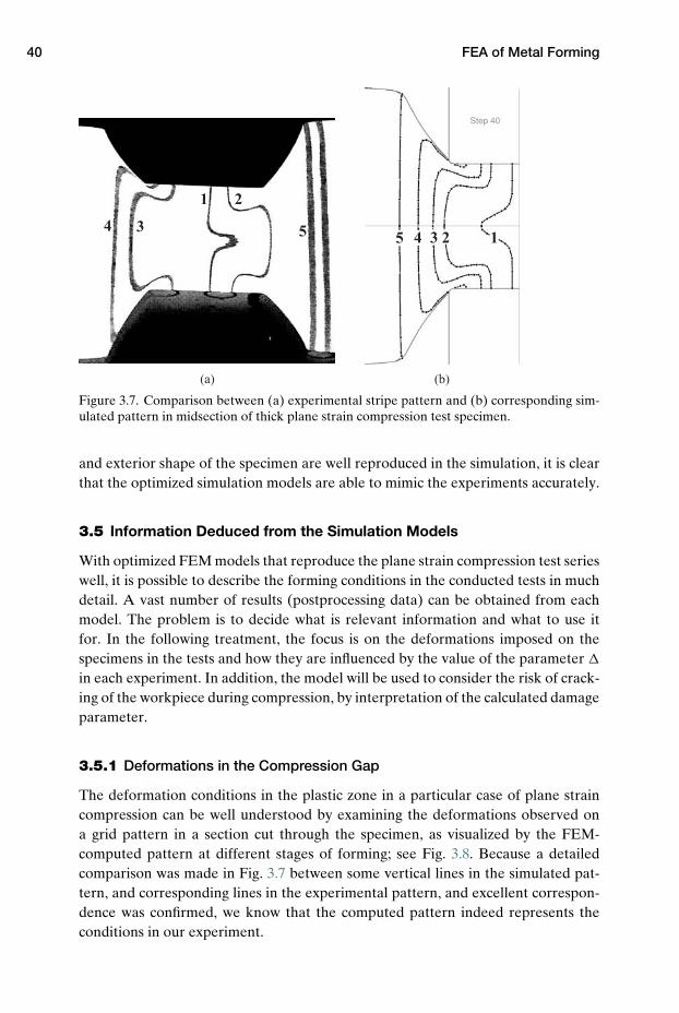
40 FEA of Metal Forming
4 3
1 2
55 4 3 2 1
Step 40
(a) (b)
Figure 3.7. Comparison between (a) experimental stripe pattern and (b) corresponding sim-ulated pattern in midsection of thick plane strain compression test specimen.
and exterior shape of the specimen are well reproduced in the simulation, it is clearthat the optimized simulation models are able to mimic the experiments accurately.
3.5 Information Deduced from the Simulation Models
With optimized FEM models that reproduce the plane strain compression test serieswell, it is possible to describe the forming conditions in the conducted tests in muchdetail. A vast number of results (postprocessing data) can be obtained from eachmodel. The problem is to decide what is relevant information and what to use itfor. In the following treatment, the focus is on the deformations imposed on thespecimens in the tests and how they are influenced by the value of the parameter �
in each experiment. In addition, the model will be used to consider the risk of crack-ing of the workpiece during compression, by interpretation of the calculated damageparameter.
3.5.1 Deformations in the Compression Gap
The deformation conditions in the plastic zone in a particular case of plane straincompression can be well understood by examining the deformations observed ona grid pattern in a section cut through the specimen, as visualized by the FEM-computed pattern at different stages of forming; see Fig. 3.8. Because a detailedcomparison was made in Fig. 3.7 between some vertical lines in the simulated pat-tern, and corresponding lines in the experimental pattern, and excellent correspon-dence was confirmed, we know that the computed pattern indeed represents theconditions in our experiment.
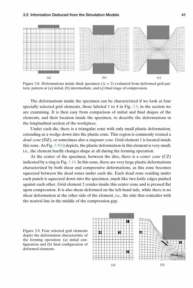
3.5 Information Deduced from the Simulation Models 41
(a) (b) (c)
Figure 3.8. Deformations inside thick specimen (� = 2) evaluated from deformed grid pat-tern: pattern at (a) initial, (b) intermediate, and (c) final stage of compression.
The deformations inside the specimen can be characterized if we look at fourspecially selected grid elements, those labeled 1 to 4 in Fig. 3.9, in the section weare examining. It is then easy from comparison of initial and final shapes of theelements, and their location inside the specimen, to describe the deformations inthe longitudinal section of the workpiece.
Under each die, there is a triangular zone with only small plastic deformation,extending as a wedge down into the plastic zone. This region is commonly termed adead zone (DZ), or sometimes also a stagnant zone. Grid element 1 is located insidethis zone. As Fig. 3.9(b) depicts, the plastic deformation in this element is very small,i.e., the element hardly changes shape at all during the forming operation.
At the center of the specimen, between the dies, there is a center zone (CZ)indicated by a ring in Fig. 3.10. In this zone, there are very large plastic deformationscharacterized by both shear and compressive deformations, as this zone becomessqueezed between the dead zones under each die. Each dead zone residing undereach punch is squeezed down into the specimen, much like two knife edges pushedagainst each other. Grid element 2 resides inside this center zone and is pressed flatupon compression. It is also shear-deformed on the left-hand side, while there is noshear deformation at the other side of the element, i.e., the side that coincides withthe neutral line in the middle of the compression gap.
(b)(a)
Figure 3.9. Four selected grid elementsdepict the deformation characteristic ofthe forming operation: (a) initial con-figuration and (b) final configuration ofdeformed elements.
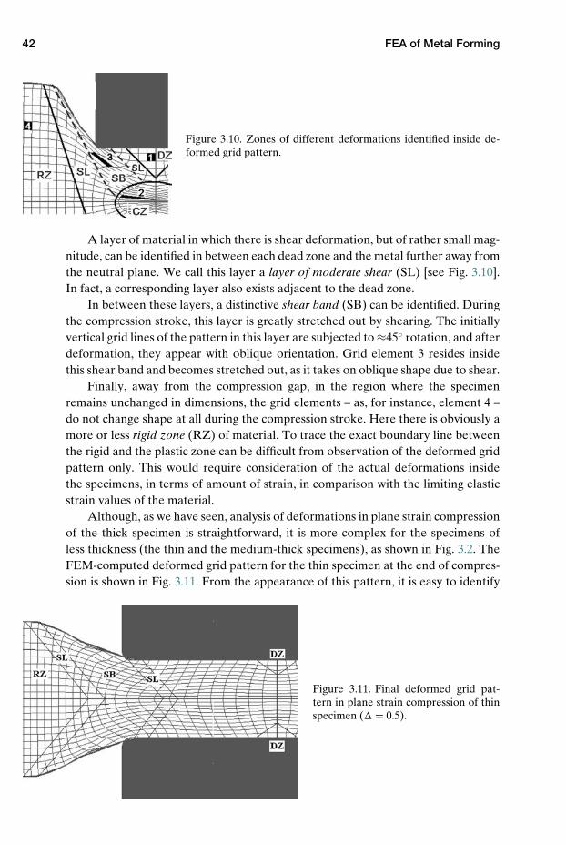
42 FEA of Metal Forming
Figure 3.10. Zones of different deformations identified inside de-formed grid pattern.
A layer of material in which there is shear deformation, but of rather small mag-nitude, can be identified in between each dead zone and the metal further away fromthe neutral plane. We call this layer a layer of moderate shear (SL) [see Fig. 3.10].In fact, a corresponding layer also exists adjacent to the dead zone.
In between these layers, a distinctive shear band (SB) can be identified. Duringthe compression stroke, this layer is greatly stretched out by shearing. The initiallyvertical grid lines of the pattern in this layer are subjected to ≈45◦ rotation, and afterdeformation, they appear with oblique orientation. Grid element 3 resides insidethis shear band and becomes stretched out, as it takes on oblique shape due to shear.
Finally, away from the compression gap, in the region where the specimenremains unchanged in dimensions, the grid elements – as, for instance, element 4 –do not change shape at all during the compression stroke. Here there is obviously amore or less rigid zone (RZ) of material. To trace the exact boundary line betweenthe rigid and the plastic zone can be difficult from observation of the deformed gridpattern only. This would require consideration of the actual deformations insidethe specimens, in terms of amount of strain, in comparison with the limiting elasticstrain values of the material.
Although, as we have seen, analysis of deformations in plane strain compressionof the thick specimen is straightforward, it is more complex for the specimens ofless thickness (the thin and the medium-thick specimens), as shown in Fig. 3.2. TheFEM-computed deformed grid pattern for the thin specimen at the end of compres-sion is shown in Fig. 3.11. From the appearance of this pattern, it is easy to identify
Figure 3.11. Final deformed grid pat-tern in plane strain compression of thinspecimen (� = 0.5).
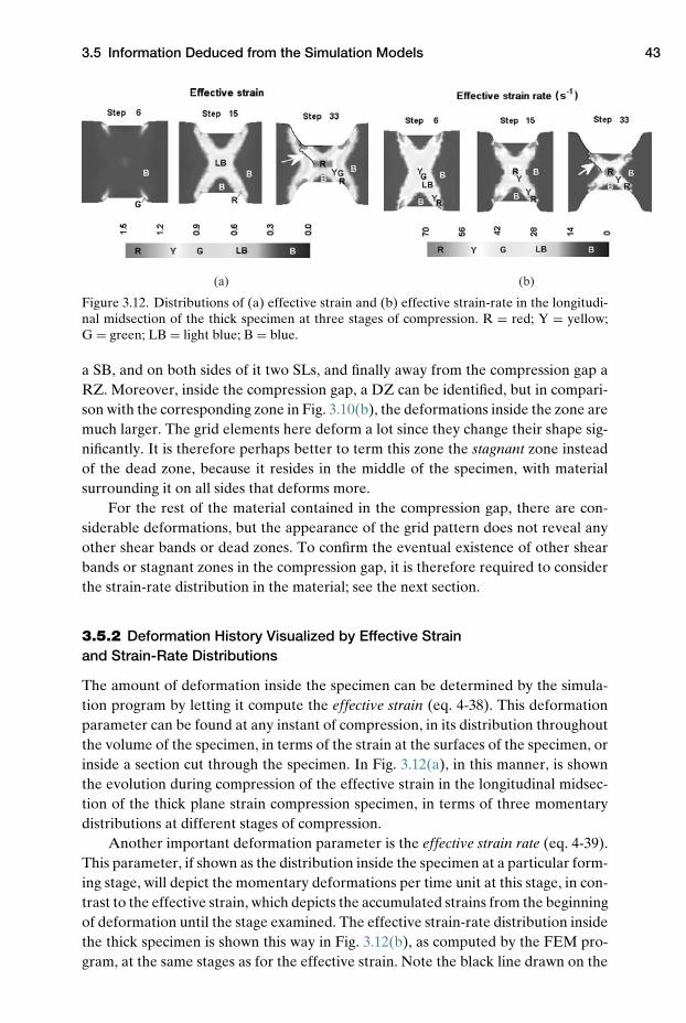
3.5 Information Deduced from the Simulation Models 43
(a) (b)
Figure 3.12. Distributions of (a) effective strain and (b) effective strain-rate in the longitudi-nal midsection of the thick specimen at three stages of compression. R = red; Y = yellow;G = green; LB = light blue; B = blue.
a SB, and on both sides of it two SLs, and finally away from the compression gap aRZ. Moreover, inside the compression gap, a DZ can be identified, but in compari-son with the corresponding zone in Fig. 3.10(b), the deformations inside the zone aremuch larger. The grid elements here deform a lot since they change their shape sig-nificantly. It is therefore perhaps better to term this zone the stagnant zone insteadof the dead zone, because it resides in the middle of the specimen, with materialsurrounding it on all sides that deforms more.
For the rest of the material contained in the compression gap, there are con-siderable deformations, but the appearance of the grid pattern does not reveal anyother shear bands or dead zones. To confirm the eventual existence of other shearbands or stagnant zones in the compression gap, it is therefore required to considerthe strain-rate distribution in the material; see the next section.
3.5.2 Deformation History Visualized by Effective Strainand Strain-Rate Distributions
The amount of deformation inside the specimen can be determined by the simula-tion program by letting it compute the effective strain (eq. 4-38). This deformationparameter can be found at any instant of compression, in its distribution throughoutthe volume of the specimen, in terms of the strain at the surfaces of the specimen, orinside a section cut through the specimen. In Fig. 3.12(a), in this manner, is shownthe evolution during compression of the effective strain in the longitudinal midsec-tion of the thick plane strain compression specimen, in terms of three momentarydistributions at different stages of compression.
Another important deformation parameter is the effective strain rate (eq. 4-39).This parameter, if shown as the distribution inside the specimen at a particular form-ing stage, will depict the momentary deformations per time unit at this stage, in con-trast to the effective strain, which depicts the accumulated strains from the beginningof deformation until the stage examined. The effective strain-rate distribution insidethe thick specimen is shown this way in Fig. 3.12(b), as computed by the FEM pro-gram, at the same stages as for the effective strain. Note the black line drawn on the
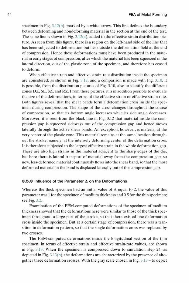
44 FEA of Metal Forming
specimen in Fig. 3.12(b), marked by a white arrow. This line defines the boundarybetween deforming and nondeforming material in the section at the end of the test.The same line is shown in Fig. 3.12(a), added to the effective strain distribution pic-ture. As seen from this figure, there is a region on the left-hand side of the line thathas been subjected to deformation but lies outside the deformation field at the endof compression. Hence these deformations must have been produced in the mate-rial in early stages of compression, after which the material has been squeezed in thelateral direction, out of the plastic zone of the specimen, and therefore has ceasedto deform.
When effective strain and effective strain-rate distribution inside the specimenare considered, as shown in Fig. 3.12, and a comparison is made with Fig. 3.10, itis possible, from the distribution pictures of Fig. 3.10, also to identify the differentzones DZ, SL, SZ, and RZ. From these pictures, it is in addition possible to evaluatethe size of the deformations, in terms of the effective strain or effective strain rate.Both figures reveal that the shear bands form a deformation cross inside the spec-imen during compression. The shape of the cross changes throughout the courseof compression, so that its bottom angle increases while its side angle decreases.Moreover, it is seen from the black line in Fig. 3.12 that material inside the com-pression gap is squeezed sideways out of the compression gap and hence moveslaterally through the active shear bands. An exception, however, is material at thevery center of the plastic zone. This material remains at the same location through-out the stroke, namely, at the intensely deforming center of the deformation cross.It is therefore subjected to the largest effective strain in the whole deformation gap.There are also high strains in the material adjacent to the sharp edges of the die,but here there is lateral transport of material away from the compression gap, sonew, less-deformed material continuously flows into the shear band, so that the mostdeformed material in the band is displaced laterally out of the compression gap.
3.5.3 Influence of the Parameter � on the Deformations
Whereas the thick specimen had an initial value of � equal to 2, the value of thisparameter was 1 for the specimen of medium thickness and 0.5 for the thin specimen;see Fig. 3.2.
Examination of the FEM-computed deformations of the specimen of mediumthickness showed that the deformations here were similar to those of the thick spec-imen throughout a large part of the stroke, so that there existed one deformationcross inside the specimen. But at a certain stage of compression, there was a tran-sition in deformation pattern, so that the single deformation cross was replaced bytwo crosses.
The FEM-computed deformations inside the longitudinal section of the thinspecimen, in terms of effective strain and effective strain-rate values, are shownin Fig. 3.13. When the specimen is compressed down to simulation step 24, asdepicted in Fig. 3.13(b), the deformations are characterized by the presence of alto-gether three deformation crosses. With the gray scale chosen in Fig. 3.13 – to depict
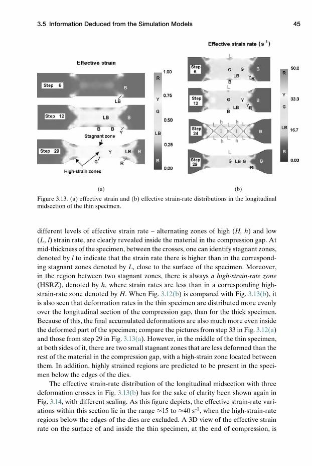
3.5 Information Deduced from the Simulation Models 45
(a) (b)
Figure 3.13. (a) effective strain and (b) effective strain-rate distributions in the longitudinalmidsection of the thin specimen.
different levels of effective strain rate – alternating zones of high (H, h) and low(L, l) strain rate, are clearly revealed inside the material in the compression gap. Atmid-thickness of the specimen, between the crosses, one can identify stagnant zones,denoted by l to indicate that the strain rate there is higher than in the correspond-ing stagnant zones denoted by L, close to the surface of the specimen. Moreover,in the region between two stagnant zones, there is always a high-strain-rate zone(HSRZ), denoted by h, where strain rates are less than in a corresponding high-strain-rate zone denoted by H. When Fig. 3.12(b) is compared with Fig. 3.13(b), itis also seen that deformation rates in the thin specimen are distributed more evenlyover the longitudinal section of the compression gap, than for the thick specimen.Because of this, the final accumulated deformations are also much more even insidethe deformed part of the specimen; compare the pictures from step 33 in Fig. 3.12(a)and those from step 29 in Fig. 3.13(a). However, in the middle of the thin specimen,at both sides of it, there are two small stagnant zones that are less deformed than therest of the material in the compression gap, with a high-strain zone located betweenthem. In addition, highly strained regions are predicted to be present in the speci-men below the edges of the dies.
The effective strain-rate distribution of the longitudinal midsection with threedeformation crosses in Fig. 3.13(b) has for the sake of clarity been shown again inFig. 3.14, with different scaling. As this figure depicts, the effective strain-rate vari-ations within this section lie in the range ≈15 to ≈40 s–1, when the high-strain-rateregions below the edges of the dies are excluded. A 3D view of the effective strainrate on the surface of and inside the thin specimen, at the end of compression, is
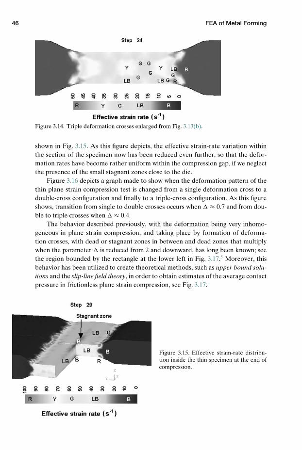
46 FEA of Metal Forming
Figure 3.14. Triple deformation crosses enlarged from Fig. 3.13(b).
shown in Fig. 3.15. As this figure depicts, the effective strain-rate variation withinthe section of the specimen now has been reduced even further, so that the defor-mation rates have become rather uniform within the compression gap, if we neglectthe presence of the small stagnant zones close to the die.
Figure 3.16 depicts a graph made to show when the deformation pattern of thethin plane strain compression test is changed from a single deformation cross to adouble-cross configuration and finally to a triple-cross configuration. As this figureshows, transition from single to double crosses occurs when � ≈ 0.7 and from dou-ble to triple crosses when � ≈ 0.4.
The behavior described previously, with the deformation being very inhomo-geneous in plane strain compression, and taking place by formation of deforma-tion crosses, with dead or stagnant zones in between and dead zones that multiplywhen the parameter � is reduced from 2 and downward, has long been known; seethe region bounded by the rectangle at the lower left in Fig. 3.17.5 Moreover, thisbehavior has been utilized to create theoretical methods, such as upper bound solu-tions and the slip-line field theory, in order to obtain estimates of the average contactpressure in frictionless plane strain compression, see Fig. 3.17.
Figure 3.15. Effective strain-rate distribu-tion inside the thin specimen at the end ofcompression.
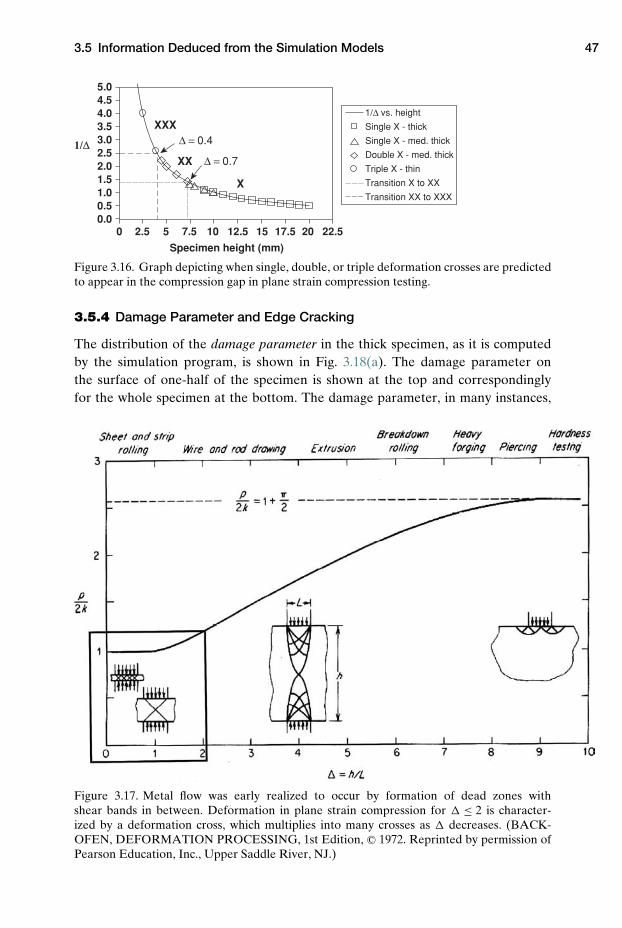
3.5 Information Deduced from the Simulation Models 47
5.0 4.5 4.0 3.5 3.0 2.5 2.0 1.5 1.0 0.5 0.0
0 2.5 5 7.5 10 12.5 15 17.5 20 22.5
Specimen height (mm)
1/∆ vs. height
Single X - thick
Single X - med. thick
Double X - med. thick
Triple X - thin
Transition X to XX
Transition XX to XXX
∆ = 0.41/∆∆ = 0.7
XXX
XX
X
Figure 3.16. Graph depicting when single, double, or triple deformation crosses are predictedto appear in the compression gap in plane strain compression testing.
3.5.4 Damage Parameter and Edge Cracking
The distribution of the damage parameter in the thick specimen, as it is computedby the simulation program, is shown in Fig. 3.18(a). The damage parameter onthe surface of one-half of the specimen is shown at the top and correspondinglyfor the whole specimen at the bottom. The damage parameter, in many instances,
Figure 3.17. Metal flow was early realized to occur by formation of dead zones withshear bands in between. Deformation in plane strain compression for � ≤ 2 is character-ized by a deformation cross, which multiplies into many crosses as � decreases. (BACK-OFEN, DEFORMATION PROCESSING, 1st Edition, c© 1972. Reprinted by permission ofPearson Education, Inc., Upper Saddle River, NJ.)
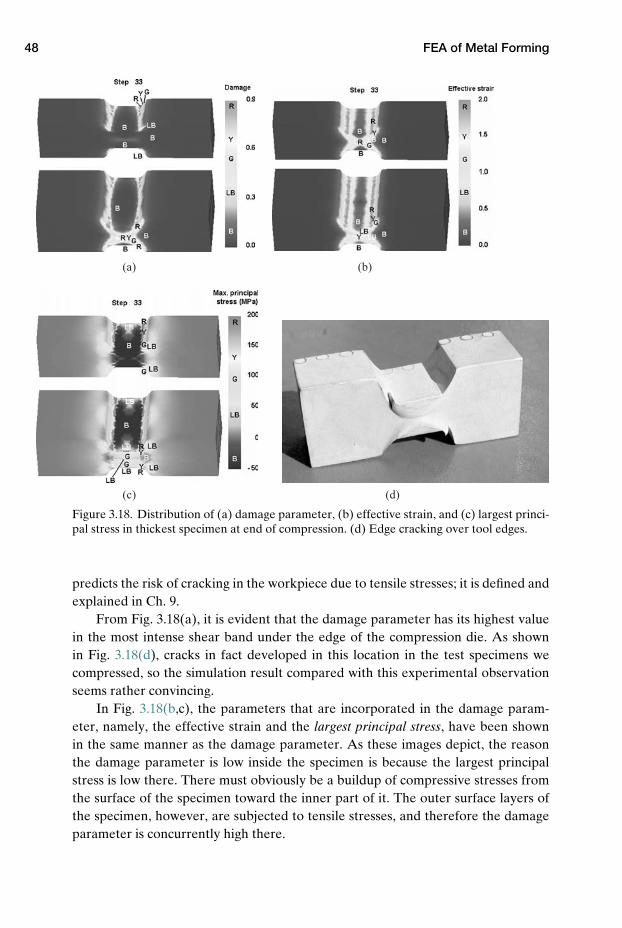
48 FEA of Metal Forming
(a) (b)
(c) (d)
Figure 3.18. Distribution of (a) damage parameter, (b) effective strain, and (c) largest princi-pal stress in thickest specimen at end of compression. (d) Edge cracking over tool edges.
predicts the risk of cracking in the workpiece due to tensile stresses; it is defined andexplained in Ch. 9.
From Fig. 3.18(a), it is evident that the damage parameter has its highest valuein the most intense shear band under the edge of the compression die. As shownin Fig. 3.18(d), cracks in fact developed in this location in the test specimens wecompressed, so the simulation result compared with this experimental observationseems rather convincing.
In Fig. 3.18(b,c), the parameters that are incorporated in the damage param-eter, namely, the effective strain and the largest principal stress, have been shownin the same manner as the damage parameter. As these images depict, the reasonthe damage parameter is low inside the specimen is because the largest principalstress is low there. There must obviously be a buildup of compressive stresses fromthe surface of the specimen toward the inner part of it. The outer surface layers ofthe specimen, however, are subjected to tensile stresses, and therefore the damageparameter is concurrently high there.
3.6 Concluding Remarks 49
3.6 Concluding Remarks
In this chapter, it has been shown how the deformation conditions in the techno-logical test plane strain compression can be characterized by FEA. The input to theFEM simulation was the flow stress data of the workpiece material and the frictiondata characterizing the shear stresses transferred through the interface between thedie and the workpiece. Such data were not readily available in this case, so sometests were run to acquire them. Flow stresses were collected in a cylinder compres-sion test. To map the sliding of the workpiece material against the die and the inter-nal metal flow, experiments were performed in which workpieces fitted with a com-bined internal and surface grid pattern were used.
A FEM model was built for the process, and the experimental grid pattern wasused to find the friction factor, which had a value of ≈0.35 in the test. The internalmetal flow of the specimen then was compared with simulated flow, and some dif-ference was found. Flow stress data were therefore slightly adjusted until the simu-lated metal flow became equal to the experimental flow. At this point, the simulatedand the experimental load–stroke curves were compared, and excellent agreementbetween the two was found. Hence, the conclusion is that the conditions in the sim-ulation models are close to those in the experiments.
The simulation was then used to study metal flow in the compression gap in thetest, run for different �-values in the range 0.5 to 2. The analysis showed that shearband formation is pronounced in plane strain compression when � = 2 and thattwo dead zones form below each die. The material at the center of the specimenis heavily deformed, as it is squeezed between the two dead zones. It was shownthat the shear bands appeared with an X shape in a longitudinal section cut throughthe specimen, i.e., a shear cross was present in the plastic zone of the specimen.Hence, for this high �, the deformations inside the compression gap were extremelynonuniform. The metal in the dead zones remained almost undeformed, while thematerial layers in between the dead zones were subjected to large deformations.
When looking at the deformations of the specimen when � = 1, the main pat-tern of deformations was similar that of the specimen with higher �, with a singledeformation cross inside the plastic zone, but there was less inhomogeneity of defor-mation. The shear cross was less intense than in the thickest specimen. Instead therewas more deformation in the dead zones. When the specimen had been compresseddown from initially 10 mm to approximately 7.4 mm height, there was a sudden tran-sition in deformation mode inside the material in the compression gap. Now doubledeformation crosses started to appear in the gap. Toward the end of compression,the deformations also became more even inside the compression gap, than before.This deformation pattern was maintained during further compression and in thebeginning when the thin specimen was compressed.
When the thin specimen had been compressed from 5 mm initial thicknessdown to approximately 4 mm, there was a new transition in deformation mode:three deformation crosses appeared in the compression gap. Throughout further
50 FEA of Metal Forming
compression of the thin specimen, deformations inside the specimen became moreuniform than before, i.e., the difference in strain rate from stagnant zones to shearbands decreased.
The conclusion thus seems to be that as the parameter � is gradually reducedfrom 2 to 0.25, as in the conducted experiments, the deformation mode changestwice as the number of deformation crosses multiplies, from a single cross to doublecrosses and finally to triple crosses. The appearance of the double and the tripledeformation crosses is not readily seen when internal grid patterns are analyzed butis well visualized in the strain-rate distributions computed by the FEM simulationmodels.
The FEA hence documents classical findings from the literature. It was earlyrecognized that the deformations in (for instance) plane strain compression arerather inhomogeneous, especially for high values of �, and that a single deforma-tion cross would be replaced by multiple crosses5 in the compression gap, when � isreduced from 1 to 0.25, as shown in Fig. 3.17.
Problems
3.1 Simulation results from cold frictionless plane strain forward extrusion areshown for a particular extrusion geometry in Fig. 3.19. Discuss how the materialdeforms in terms of deformation of grid elements, presence of deformation crosses,homogeneity of deformation, and non-steady-state or steady-state conditions forthis forming process on the basis of the given information.
3.2 Write down a short explanation to express your understanding of the followingterms used in this chapter:
(a) Metal flow (b) FEA(c) Physical metal forming simulator (d) Inverse modeling(e) Surface ring pattern (f) Shear cross(g) Dead zone (h) Stagnant zone(i) High-strain-rate zone (j) Effective strain(k) Effective strain-rate distribution (l) Upper bound solution(m) Damage parameter
3.3 Figure 9.6 shows FEM-computed distributions of some process parameters incylinder compression.
(a) Make a 3D sketch of this metal forming test, and explain how it differs fromthe plane strain compression test method.
(b) Try to interpret the given simulated distributions of process parameters onthe basis of deformations inside the specimen and the risk of tensile stresscracking.
3.4 In the middle of Fig. 19.1 is shown the deformed grid pattern obtained in a FEMsimulation model of forward extrusion of an aluminum alloy. On the basis of thisgrid pattern, discuss the following relations:
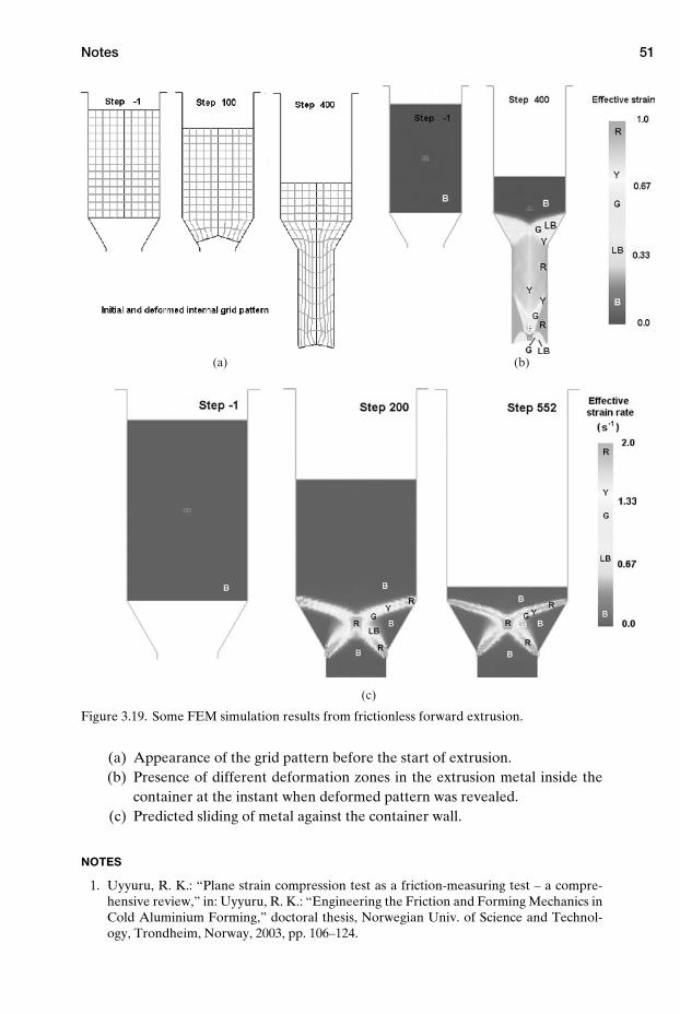
Notes 51
(a) (b)
(c)
Figure 3.19. Some FEM simulation results from frictionless forward extrusion.
(a) Appearance of the grid pattern before the start of extrusion.(b) Presence of different deformation zones in the extrusion metal inside the
container at the instant when deformed pattern was revealed.(c) Predicted sliding of metal against the container wall.
NOTES
1. Uyyuru, R. K.: “Plane strain compression test as a friction-measuring test – a compre-hensive review,” in: Uyyuru, R. K.: “Engineering the Friction and Forming Mechanics inCold Aluminium Forming,” doctoral thesis, Norwegian Univ. of Science and Technol-ogy, Trondheim, Norway, 2003, pp. 106–124.

52 FEA of Metal Forming
2. Nolte, D., and Uyyuru, R. K.: “Review and recent developments in physical model-ing of metal forming,” in: Nolte, D.: “Analysis of Aluminium Hot Forging,” doctoralthesis, Norwegian Univ. of Science and Technology, Trondheim, Norway, 2005, pp. 89–115.
3. Valberg, H., Uyyuru, R. K., and Lefstad, M.: “Analysis of deformations in plane straincompression using advanced grid pattern technique,” Proc. 9th Esaform Conf., Glasgow,2006, pp. 891–894.
4. NTNU is an abbreviation for the Norwegian University of Science and Technology.5. Backofen, W. A.: “Deformation Processing,” Addison-Wesley, Reading, MA, 1972,
p. 135.
REFERENCES
Bay, N., Wanheim, T, Danckert, J., and Nielsen, K. B.: “An appraisal of numerical and phys-ical modelling for prediction of metal forming processes,” Proc. 15th. Risø Int. Symp. onMaterials Science, 1994, pp. 1–32.
Li, G., Jinn, J. T., Wu, W. T., and Oh, S. I.: “Recent development and applications of three-dimensional finite element modelling in bulk forming processes,” J. Materials ProcessingTechnology, Vol. 113, 2001, pp. 40–45.
Mielnik, E. M.: “Metalworking Science and Engineering,” McGraw-Hill, New York, 1991,p. 494.
Schey, J. A.: “Introduction to Manufacturing Processes,” McGraw-Hill, 1977, pp. 108–111.Shirgaokar, M., Yadav, A., and Taylan, A.: “Simulation and optimization of metal forming
processes,” 19th Umformtechnisches Kolloquium Hannover, 27–28 Feb. 2008, pp. 173–186.Wagoner, R. H., and Chenot, J.-L.: “Metal Forming Analysis,” Cambridge University Press,
2001.
4 Theory
Because metal forming produces elastic and plastic deformations in the workpiecematerial and elastic deformations in the dies, an in-depth study of the metal formingprocess will require the determination of stresses and strains in the workpiece andthe tooling. In addition, one needs to know some basic topics from the theory ofelasticity and plasticity. In this chapter, a short introduction to this theory is there-fore given. Because of the rather shallow treatment here, readers who are unfamiliarwith this theory are referred to other textbooks1–3 for a more profound study.
4.1 Stresses
During metal forming the workpiece is deformed plastically by forces transferredfrom the die to the workpiece. A successful forming operation requires that therebe plastic deformations in the workpiece, so that it changes shape permanently andconforms to the geometry of the die, while the die remains in the elastic state. If thedie material becomes plasticized, the situation is one of overloading of the tooling,and the die geometry will gradually change because of the excessive forming loads.This means that the correct geometry of the formed component no longer can bemaintained, so to continue appropriate metal forming, the dies must be replaced bynew dies that can work the material while remaining in the elastic state.
4.1.1 The Stress Concept
Stress is defined as force per unit of area and refers to a particular point in a material.Suppose a force dF is directed at an angle to a surface dA at a particular place insidea material. If the area is made smaller until it approaches toward zero, the areawill become a point. In addition, a stress will act on this point, directed in the samedirection as the force, with magnitude σ = dF/dA. This stress can be decomposedinto two components, a shear stress and a normal stress, as expressed by:
τ = dFt
dA(4-1)
σn = dFn
dA(4-2)
53
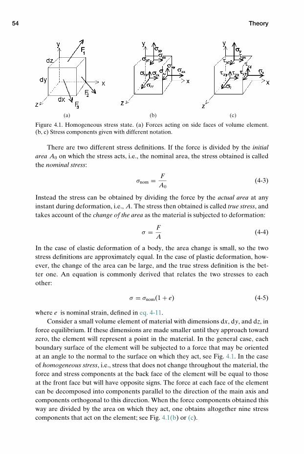
54 Theory
(a) (b) (c)
Figure 4.1. Homogeneous stress state. (a) Forces acting on side faces of volume element.(b, c) Stress components given with different notation.
There are two different stress definitions. If the force is divided by the initialarea A0 on which the stress acts, i.e., the nominal area, the stress obtained is calledthe nominal stress:
σnom = FA0
(4-3)
Instead the stress can be obtained by dividing the force by the actual area at anyinstant during deformation, i.e., A. The stress then obtained is called true stress, andtakes account of the change of the area as the material is subjected to deformation:
σ = FA
(4-4)
In the case of elastic deformation of a body, the area change is small, so the twostress definitions are approximately equal. In the case of plastic deformation, how-ever, the change of the area can be large, and the true stress definition is the bet-ter one. An equation is commonly derived that relates the two stresses to eachother:
σ = σnom(1 + e) (4-5)
where e is nominal strain, defined in eq. 4-11.Consider a small volume element of material with dimensions dx, dy, and dz, in
force equilibrium. If these dimensions are made smaller until they approach towardzero, the element will represent a point in the material. In the general case, eachboundary surface of the element will be subjected to a force that may be orientedat an angle to the normal to the surface on which they act, see Fig. 4.1. In the caseof homogeneous stress, i.e., stress that does not change throughout the material, theforce and stress components at the back face of the element will be equal to thoseat the front face but will have opposite signs. The force at each face of the elementcan be decomposed into components parallel to the direction of the main axis andcomponents orthogonal to this direction. When the force components obtained thisway are divided by the area on which they act, one obtains altogether nine stresscomponents that act on the element; see Fig. 4.1(b) or (c).
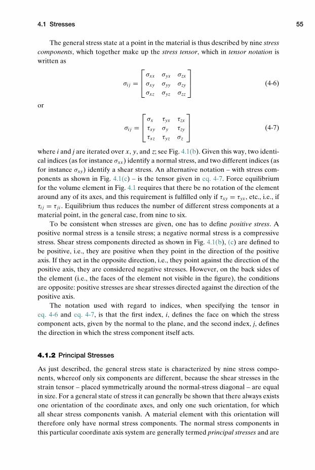
4.1 Stresses 55
The general stress state at a point in the material is thus described by nine stresscomponents, which together make up the stress tensor, which in tensor notation iswritten as
σi j =
σxx σyx σzx
σxy σyy σzy
σxz σyz σzz
(4-6)
or
σi j =
σx τyx τzx
τxy σy τzy
τxz τyz σz
(4-7)
where i and j are iterated over x, y, and z; see Fig. 4.1(b). Given this way, two identi-cal indices (as for instance σxx) identify a normal stress, and two different indices (asfor instance σxy) identify a shear stress. An alternative notation – with stress com-ponents as shown in Fig. 4.1(c) – is the tensor given in eq. 4-7. Force equilibriumfor the volume element in Fig. 4.1 requires that there be no rotation of the elementaround any of its axes, and this requirement is fulfilled only if τxy = τyx, etc., i.e., ifτi j = τ j i . Equilibrium thus reduces the number of different stress components at amaterial point, in the general case, from nine to six.
To be consistent when stresses are given, one has to define positive stress. Apositive normal stress is a tensile stress; a negative normal stress is a compressivestress. Shear stress components directed as shown in Fig. 4.1(b), (c) are defined tobe positive, i.e., they are positive when they point in the direction of the positiveaxis. If they act in the opposite direction, i.e., they point against the direction of thepositive axis, they are considered negative stresses. However, on the back sides ofthe element (i.e., the faces of the element not visible in the figure), the conditionsare opposite: positive stresses are shear stresses directed against the direction of thepositive axis.
The notation used with regard to indices, when specifying the tensor ineq. 4-6 and eq. 4-7, is that the first index, i, defines the face on which the stresscomponent acts, given by the normal to the plane, and the second index, j, definesthe direction in which the stress component itself acts.
4.1.2 Principal Stresses
As just described, the general stress state is characterized by nine stress compo-nents, whereof only six components are different, because the shear stresses in thestrain tensor – placed symmetrically around the normal-stress diagonal – are equalin size. For a general state of stress it can generally be shown that there always existsone orientation of the coordinate axes, and only one such orientation, for whichall shear stress components vanish. A material element with this orientation willtherefore only have normal stress components. The normal stress components inthis particular coordinate axis system are generally termed principal stresses and are
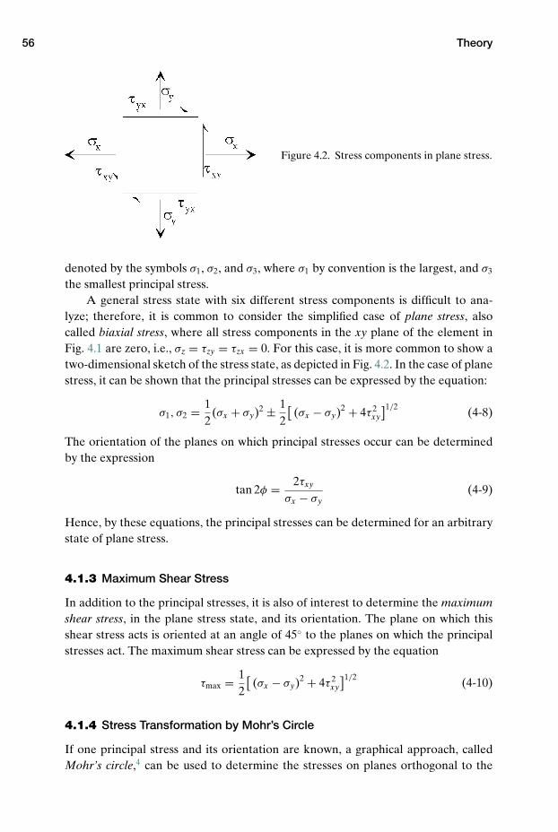
56 Theory
Figure 4.2. Stress components in plane stress.
denoted by the symbols σ1, σ2, and σ3, where σ1 by convention is the largest, and σ3
the smallest principal stress.A general stress state with six different stress components is difficult to ana-
lyze; therefore, it is common to consider the simplified case of plane stress, alsocalled biaxial stress, where all stress components in the xy plane of the element inFig. 4.1 are zero, i.e., σz = τzy = τzx = 0. For this case, it is more common to show atwo-dimensional sketch of the stress state, as depicted in Fig. 4.2. In the case of planestress, it can be shown that the principal stresses can be expressed by the equation:
σ1, σ2 = 12
(σx + σy)2 ± 12
[(σx − σy)2 + 4τ 2
xy
]1/2 (4-8)
The orientation of the planes on which principal stresses occur can be determinedby the expression
tan 2φ = 2τxy
σx − σy(4-9)
Hence, by these equations, the principal stresses can be determined for an arbitrarystate of plane stress.
4.1.3 Maximum Shear Stress
In addition to the principal stresses, it is also of interest to determine the maximumshear stress, in the plane stress state, and its orientation. The plane on which thisshear stress acts is oriented at an angle of 45◦ to the planes on which the principalstresses act. The maximum shear stress can be expressed by the equation
τmax = 12
[(σx − σy)2 + 4τ 2
xy
]1/2 (4-10)
4.1.4 Stress Transformation by Mohr’s Circle
If one principal stress and its orientation are known, a graphical approach, calledMohr’s circle,4 can be used to determine the stresses on planes orthogonal to the
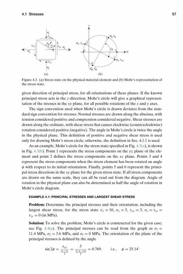
4.1 Stresses 57
τφ
σ
τ
σφ
(a) (b)
4
6
1
5
3
2
2φ
σx, τxy
σy, τyxτyx
τyx
τxy
τyx σφ,τφ
σ′φ,τ′φ
σy
σy
σx
σy
φ
Figure 4.3. (a) Stress state on the physical material element and (b) Mohr’s representation ofthe stress state.
given direction of principal stress, for all orientations of these planes. If the knownprincipal stress acts in the z-direction, Mohr’s circle will give a graphical represen-tation of the stresses in the xy plane, for all possible rotations of the x and y axes.
The sign convention used when Mohr’s circle is drawn deviates from the stan-dard sign convention for stresses. Normal stresses are drawn along the abscissa, withtension considered positive and compression considered negative. Shear stresses aredrawn along the ordinate, with shear stress that causes clockwise (counterclockwise)rotation considered positive (negative). The angle in Mohr’s circle is twice the anglein the physical plane. This definition of positive and negative shear stress is usedonly for drawing Mohr’s stress circle; otherwise, the definition in Sec. 4.1.1 is used.
As an example, Mohr’s circle for the stress state specified in Fig. 4.3(a), is shownin Fig. 4.3(b). Point 1 represents the stress components on the yz plane of the ele-ment and point 2 defines the stress components on the xz plane. Points 3 and 4represent the stress components when the stress element has been rotated an angleφ with respect to its initial orientation. Finally, points 5 and 6 represent the princi-pal stress directions in the xy plane for the given stress state. If all stress componentsare drawn on the same scale, they can all be read out from the diagram. Angle ofrotation in the physical plane can also be determined as half the angle of rotation inMohr’s circle diagram.
EXAMPLE 4.1: PRINCIPAL STRESSES AND LARGEST SHEAR STRESS
Problem: Determine the principal stresses and their orientation, including thelargest shear stress, for the stress state σx = 10, σy = 5, τxy = 3, σz = τzx =τzy = 0 (in MPa).
Solution: To solve the problem, Mohr’s circle is constructed for the given case;see Fig. 4.4(a). The principal stresses can be read from the graph as σ1 =11.4 MPa, σ2 = 3.6 MPa, and σ3 = 0 MPa. The orientation of the plane of theprincipal stresses is defined by the angle
sin 2φ = τxyσ1−σ2
2
= 311.4−3.6
2
= 0.769, i.e., φ = 25.14◦
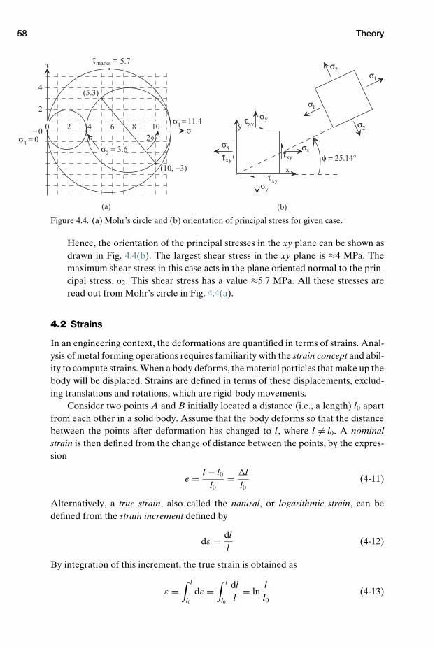
58 Theory
2φ
τ
σ
(a)
σ3 = 0
2
4
(b)
σ2 = 3.6
σ1 = 11.4y
φ = 25.14°x
σx
σ2
σ2
σ1
σ1
σy
σy
σx
(5.3)
0 2 4 6 8 10
5.7
Figure 4.4. (a) Mohr’s circle and (b) orientation of principal stress for given case.
Hence, the orientation of the principal stresses in the xy plane can be shown asdrawn in Fig. 4.4(b). The largest shear stress in the xy plane is ≈4 MPa. Themaximum shear stress in this case acts in the plane oriented normal to the prin-cipal stress, σ2. This shear stress has a value ≈5.7 MPa. All these stresses areread out from Mohr’s circle in Fig. 4.4(a).
4.2 Strains
In an engineering context, the deformations are quantified in terms of strains. Anal-ysis of metal forming operations requires familiarity with the strain concept and abil-ity to compute strains. When a body deforms, the material particles that make up thebody will be displaced. Strains are defined in terms of these displacements, exclud-ing translations and rotations, which are rigid-body movements.
Consider two points A and B initially located a distance (i.e., a length) l0 apartfrom each other in a solid body. Assume that the body deforms so that the distancebetween the points after deformation has changed to l, where l �= l0. A nominalstrain is then defined from the change of distance between the points, by the expres-sion
e = l − l0
l0= �l
l0(4-11)
Alternatively, a true strain, also called the natural, or logarithmic strain, can bedefined from the strain increment defined by
dε = dll
(4-12)
By integration of this increment, the true strain is obtained as
ε =∫ l
l0
dε =∫ l
l0
dll
= lnll0
(4-13)
4.2 Strains 59
In the case of small deformations, as, for instance, elastic deformations in metals, thedifference between the two strain definitions is small, i.e., nominal and true strainare approximately equal. But for large deformations, there is a significant differencebetween nominal and true strain; see Example 4.2.
True strains are additive, in contrast to nominal strains, which cannot be added;see Example 4.3. For a forming operation performed in successive stages, it is advan-tageous if true strains are used, because the total strains in the process then can beobtained as the sum of the strains in the individual stages. Another advantage is thatone can compare deformations in compression and tension, because correspond-ing deformations in these two opposite deformation modes will have the same truestrain value with the opposite sign; see Problem 4.1. Finally, when using true strains,the sum of the three normal strains in the plastically deforming object correspondsto the volume change of the object, which, for metals that exhibit volume constancy,will equal zero. To transform true strain into a corresponding nominal strain, or viceversa, the following expression can be used:
ε = ln(1 + e) (4-14)
EXAMPLE 4.2: DIFFERENCE BETWEEN NOMINAL AND TRUE STRAIN
Problem: Compute the ratio of true to nominal strain for the following truestrain values:
e = 0.001, 0.01, 0.1, 0.5
Solution: True strains are computed from nominal strain values using eq. 4-14.The ratio between the two strains definitions can then be determined with thefollowing result:
e = 0.001 ⇒ eε
= 0.9995, e = 0.01 ⇒ eε
= 0.995,
e = 0.1 ⇒ eε
= 0.953, e = 0.5 ⇒ eε
= 0.811
This shows that nominal and true strains are approximately equal for lowstrain values and that nominal strain is significantly larger than the true strainfor large strains. So, in the case of elastic deformations, where e ≤ 0.01, itdoes not make much difference whether strain is expressed as nominal or truestrain.
EXAMPLE 4.3: TRUE STRAINS CAN BE ADDED
Problem: A rod with initial length l0 = 10 cm is rolled down in three rollingsteps. The length after each step is measured to be l1 = 12 cm, l2 = 15 cm, andl3 = 20 cm, respectively. Compute average strains in each step and in the wholeprocess. Apply both nominal and true strain definitions.
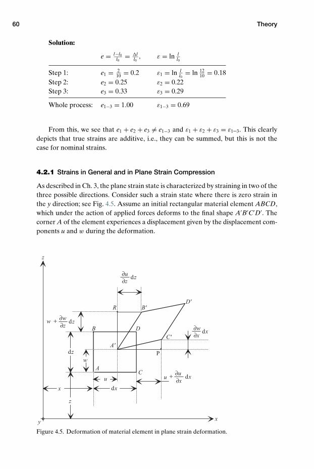
60 Theory
Solution:
e = l−l0l0
= �ll0
, ε = ln ll0
Step 1: e1 = 210 = 0.2 ε1 = ln l
l0= ln 12
10 = 0.18Step 2: e2 = 0.25 ε2 = 0.22Step 3: e3 = 0.33 ε3 = 0.29
Whole process: e1−3 = 1.00 ε1−3 = 0.69
From this, we see that e1 + e2 + e3 �= e1−3 and ε1 + ε2 + ε3 = ε1–3. This clearlydepicts that true strains are additive, i.e., they can be summed, but this is not thecase for nominal strains.
4.2.1 Strains in General and in Plane Strain Compression
As described in Ch. 3, the plane strain state is characterized by straining in two of thethree possible directions. Consider such a strain state where there is zero strain inthe y direction; see Fig. 4.5. Assume an initial rectangular material element ABCD,which under the action of applied forces deforms to the final shape A′B′C′D′. Thecorner A of the element experiences a displacement given by the displacement com-ponents u and w during the deformation.
∂w
∂u
∂z
∂z
+
z
R B'
B
A'
D'
A
C'
C
P
D
u
dx
dz
dz
dz
∂w∂x
dx
w
w
∂u∂x
+ dx
x y
z
x
u
Figure 4.5. Deformation of material element in plane strain deformation.
4.2 Strains 61
The deformations of the body can be quantified by means of nominal normalstrains and shear strains. These strains will be ex, ez, and exz = ezx, of which the firstis defined as follows:
ex = dεx = A′C′ − ACAC
= A′C′
AC− 1 ≈ A′ P
AC− 1 (4-15)
Let us assume that the deformations are small, so that A′ P ≈ A′C′. As shown byeq. 4-15, this expression at the same time represents the strain increment in the caseof small deformations. The normal strain can also be expressed as
ex = dx + (u + ∂u∂x dx) − u
dx− 1 = ∂u
∂x(4-16)
Using a corresponding approach, the other normal strain can be determined as
ez = ∂w
∂z(4-17)
and the shear strain can be determined as
exz = ezx = 12γxz (4-18)
where γxz = ∠P A′C′ + ∠RA′C′. From Fig. 4.5, we can see that for small deforma-tions ∠P A′C′ can be expressed as
∠P A′C′ = arctanPC′
A′ P′ = arctan∂w∂x dx
dx + u + ∂u∂x dx − u
= arctan∂w∂x
1 + ∂u∂x
≈ arctan∂w
∂x= ∂w
∂x(4-19)
because ∂u/∂x � 1. Correspondingly, it can be shown that ∠RA′ B′ = ∂u/∂z.Hence, the shear strain can be expressed as
exz = ezx = 12γxz = 1
2
(∂w
∂x+ ∂u
∂z
)(4-20)
For the general three-dimensional case, there are three additional nominal straincomponents. Like the preceding strains, they can be determined as
ey = ∂v∂y
(4-21)
exy = 12γxy = 1
2
(∂u∂y
+ ∂v∂x
)(4-22)
eyz = 12γyz = 1
2
(∂v∂z
+ ∂w
∂y
)(4-23)
Note that in the preceding treatment one applies two different definitions of shearstrain, i.e., in one case the engineering strain, γ , and in the other case strain as thetensor value, e = γ /2.
62 Theory
4.2.3 Strain as a Tensor
Strains can be given in tensor notation corresponding to that for stresses. Then theshear strain must be defined by the tensor values specified in eqs. 4-16 and 4-17 andeqs. 4-20 to 4-23:
ei j =
exx eyx ezx
exy eyy exy
exz eyz ezz
(4-24)
When deformations are small, as in the case of elastic deformations, or when thestrain increment dε is used, both nominal and true strains will be tensor quantities.Note that the strain tensor is analogous to the stress tensor; compare eq. 4-24 witheq. 4-6.
4.2.4 Analogy between Stress and Strain
Stresses and strains can both be expressed by similar tensors, and there are in addi-tion a number of other similarities between them. For a strain state there is one,and only one, orientation of the coordinate system that causes shear strains to dis-appear, as was the case for a stress state. The strain state in which this occurs iscalled the principal strain state, analogous to the principal stress state, and the nor-mal strains in this state are called principal strains. Moreover, the principal values ofnormal strains, and the orientation of the principal strain state, are determined byequations similar those for stress:
Principal strain (analog of eq. 4-8):
e1, e2 = 12
(ex + ey)2 ± 12
[(ex − ey)2 + 4e2
xy
]1/2(4-25)
Maximum shear strain (analog of eq. 4-10):
emax = 12γmax = 1
2
[(ex − ey)2 + 4e2
xy
]1/2(4-26)
As for stresses, a Mohr’s circle can be drawn for the plane strain state. This circlegraphically displays the variation of strain values with orientation of the coordinatesystem, when rotated around its origin. In Mohr’s circle, normal strains are plottedalong the abscissa axis, and shear strains in terms of the tensor strain, e = 1
2γ , alongthe ordinate axis. If the principal strains are known, for the case of plane strain, onecan find from this circle the strain components in any arbitrary direction rotated byan angle θ relative to the plane of the principal stresses. This is done by use of theequations
ex, ey = 12
(e1 + e2) ± 12
(e1 − e2) cos 2θ (4-27)
γxy = (e1 − e2) sin 2θ (4-28)
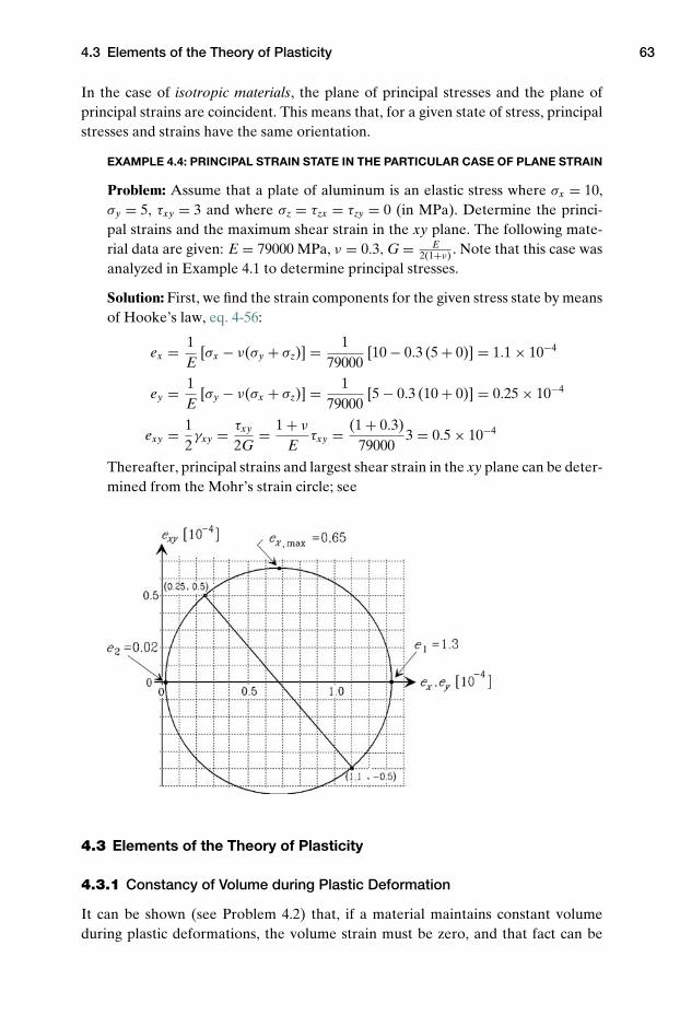
4.3 Elements of the Theory of Plasticity 63
In the case of isotropic materials, the plane of principal stresses and the plane ofprincipal strains are coincident. This means that, for a given state of stress, principalstresses and strains have the same orientation.
EXAMPLE 4.4: PRINCIPAL STRAIN STATE IN THE PARTICULAR CASE OF PLANE STRAIN
Problem: Assume that a plate of aluminum is an elastic stress where σx = 10,σy = 5, τxy = 3 and where σz = τzx = τzy = 0 (in MPa). Determine the princi-pal strains and the maximum shear strain in the xy plane. The following mate-rial data are given: E = 79000 MPa, ν = 0.3, G = E
2(1+ν) . Note that this case wasanalyzed in Example 4.1 to determine principal stresses.
Solution: First, we find the strain components for the given stress state by meansof Hooke’s law, eq. 4-56:
ex = 1E
[σx − ν(σy + σz)] = 179000
[10 − 0.3 (5 + 0)] = 1.1 × 10⁻⁴
ey = 1E
[σy − ν(σx + σz)] = 179000
[5 − 0.3 (10 + 0)] = 0.25 × 10⁻⁴
exy = 12γxy = τxy
2G= 1 + ν
Eτxy = (1 + 0.3)
790003 = 0.5 × 10⁻⁴
Thereafter, principal strains and largest shear strain in the xy plane can be deter-mined from the Mohr’s strain circle; see
4.3 Elements of the Theory of Plasticity
4.3.1 Constancy of Volume during Plastic Deformation
It can be shown (see Problem 4.2) that, if a material maintains constant volumeduring plastic deformations, the volume strain must be zero, and that fact can be
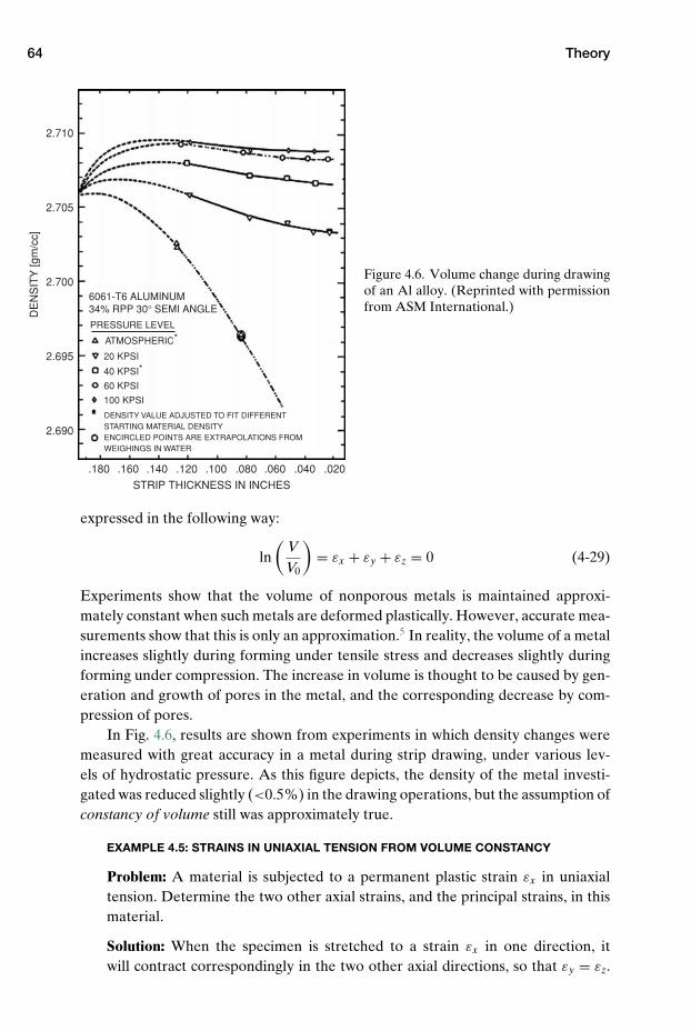
64 Theory
2.710
2.705
2.700
2.695
2.690
DE
NS
ITY
[gm
/cc]
STRIP THICKNESS IN INCHES
.180 .160 .140 .120 .100 .080 .060 .040 .020
6061-T6 ALUMINUM 34% RPP 30° SEMI ANGLE PRESSURE LEVEL
ATMOSPHERIC*
40 KPSI*20 KPSI
60 KPSI
100 KPSI
DENSITY VALUE ADJUSTED TO FIT DIFFERENT STARTING MATERIAL DENSITY ENCIRCLED POINTS ARE EXTRAPOLATIONS FROM WEIGHINGS IN WATER
Figure 4.6. Volume change during drawingof an Al alloy. (Reprinted with permissionfrom ASM International.)
expressed in the following way:
ln(
VV0
)= εx + εy + εz = 0 (4-29)
Experiments show that the volume of nonporous metals is maintained approxi-mately constant when such metals are deformed plastically. However, accurate mea-surements show that this is only an approximation.5 In reality, the volume of a metalincreases slightly during forming under tensile stress and decreases slightly duringforming under compression. The increase in volume is thought to be caused by gen-eration and growth of pores in the metal, and the corresponding decrease by com-pression of pores.
In Fig. 4.6, results are shown from experiments in which density changes weremeasured with great accuracy in a metal during strip drawing, under various lev-els of hydrostatic pressure. As this figure depicts, the density of the metal investi-gated was reduced slightly (<0.5%) in the drawing operations, but the assumption ofconstancy of volume still was approximately true.
EXAMPLE 4.5: STRAINS IN UNIAXIAL TENSION FROM VOLUME CONSTANCY
Problem: A material is subjected to a permanent plastic strain εx in uniaxialtension. Determine the two other axial strains, and the principal strains, in thismaterial.
Solution: When the specimen is stretched to a strain εx in one direction, itwill contract correspondingly in the two other axial directions, so that εy = εz.
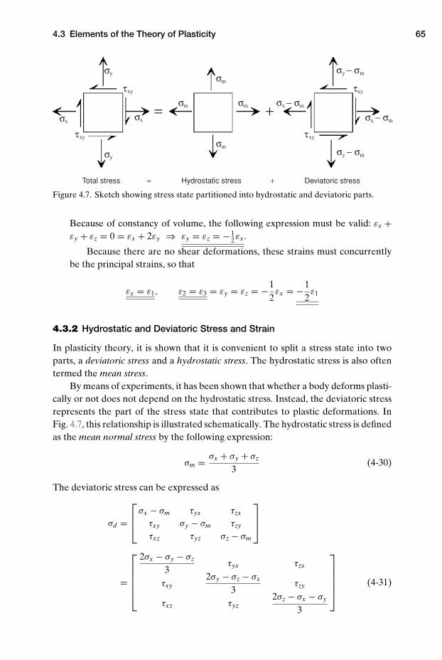
4.3 Elements of the Theory of Plasticity 65
Total stress
= +
= Hydrostatic stress Deviatoric stress+
Figure 4.7. Sketch showing stress state partitioned into hydrostatic and deviatoric parts.
Because of constancy of volume, the following expression must be valid: εx +εy + εz = 0 = εx + 2εy ⇒ εy = εz = − 1
2εx.
Because there are no shear deformations, these strains must concurrentlybe the principal strains, so that
εx = ε1, ε2 = ε3 = εy = εz = −12εx = −1
2ε1
4.3.2 Hydrostatic and Deviatoric Stress and Strain
In plasticity theory, it is shown that it is convenient to split a stress state into twoparts, a deviatoric stress and a hydrostatic stress. The hydrostatic stress is also oftentermed the mean stress.
By means of experiments, it has been shown that whether a body deforms plasti-cally or not does not depend on the hydrostatic stress. Instead, the deviatoric stressrepresents the part of the stress state that contributes to plastic deformations. InFig. 4.7, this relationship is illustrated schematically. The hydrostatic stress is definedas the mean normal stress by the following expression:
σm = σx + σy + σz
3(4-30)
The deviatoric stress can be expressed as
σd =
σx − σm τyx τzx
τxy σy − σm τzy
τxz τyz σz − σm
=
2σx − σy − σz
3τyx τzx
τxy2σy − σz − σx
3τzy
τxz τyz2σz − σx − σy
3
(4-31)
66 Theory
In view of the analogy between stresses and strains, the strain state can alsobe partitioned in two parts, one part that contributes to volume change, called thehydrostatic strain, or mean strain, and another part, called the deviatoric strain, thatcauses change of shape of the strained body. Corresponding to eqs. 4-30 and 4-31,the nominal hydrostatic and the nominal deviatoric strains are given as
em = ex + ey + ez
3(4-32)
ed =
ex − em eyx ezx
exy ey − em ezy
exz eyz ez − em
=
2ex − ey − ez
3eyx ezx
exyey − ez − ex
3ezy
exz eyz2ez − ex − ey
3
(4-33)
In these equations, the nominal values of the strain components are used, but alter-natively they can be replaced by true strain values.
EXAMPLE 4.6: EFFECT OF INCREASED HYDROSTATIC STRESS ON PLASTIC YIELD
Problem: A stress condition characterized by the principal stresses σ1 = 80,σ2 = 45, σ3 = −30 MPa does not cause plastic deformation in a particular mate-rial. What happens if this material in addition is exposed to a fluid pressure of50 MPa?
Solution: The diameters of the Mohr’s circles for the initial stress condition (seeunnumbered figure), are
d1 = σ1 − σ2 = 80 − 45 = 35, d2 = σ2 − σ3 = 45 − (−30) = 75,
d3 = σ1 − σ3 = 80 − (−30) = 110
The principal stresses for the pressurized condition are
σ1,pr = σ1 − 50 = 80 − 50 = 30σ2,pr = σ2 − 50 = 45 − 50 = −5σ3,pr = σ3 − 50 = −30 − 50 = −80
From the pressurized principal stresses, the new diameters of the Mohr’s circlesare determined as
d1,pr = σ1,pr − σ2,pr = 30 − (−5) = 35d2,pr = σ2,pr − σ3,pr = −5 − (−80) = 75d3,pr = σ1,pr − σ3,pr = 30 − (−80) = 110
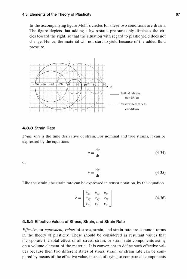
4.3 Elements of the Theory of Plasticity 67
In the accompanying figure Mohr’s circles for these two conditions are drawn.The figure depicts that adding a hydrostatic pressure only displaces the cir-cles toward the right, so that the situation with regard to plastic yield does notchange. Hence, the material will not start to yield because of the added fluidpressure.
4.3.3 Strain Rate
Strain rate is the time derivative of strain. For nominal and true strains, it can beexpressed by the equations
e = dedt
(4-34)
or
ε = dε
dt(4-35)
Like the strain, the strain rate can be expressed in tensor notation, by the equation
e =
exx eyx ezx
exy eyy ezy
exz eyz ezz
(4-36)
4.3.4 Effective Values of Stress, Strain, and Strain Rate
Effective, or equivalent, values of stress, strain, and strain rate are common termsin the theory of plasticity. These should be considered as resultant values thatincorporate the total effect of all stress, strain, or strain rate components actingon a volume element of the material. It is convenient to define such effective val-ues because then two different states of stress, strain, or strain rate can be com-pared by means of the effective value, instead of trying to compare all components
68 Theory
separately. For the general state of stress, strain, or strain rate, these effective valuesare defined as follows:
Effective stress:
σ = 1√2
[(σx − σy)2 + (σy − σz)
2 + (σz − σx)2 + 6(τ 2
xy + τ 2yz + τ 2
xz
)]1/2 (4-37)
Effective strain:
ε ={
23
[ε2
x + ε2y + ε2
z + 2(ε2
xy + ε2yz + ε2
zx
)]}1/2
(4-38)
Effective strain rate:
˙ε ={
23
[ε2
x + ε2y + ε2
z + 2(ε2
xy + ε2yz + ε2
zx
)]}1/2
(4-39)
Often eq. 4-38 and eq. 4-39 are expressed as strain or strain-rate increments (dε,d ˙ε), instead of strains (ε, ˙ε), to show that they evolve after the end of the initialelastic deformation. For large plastic deformations, however, elastic deformationsare negligible in comparison with plastic deformations, and their contributions canbe neglected.
The flow curve obtained for an arbitrary complex deformation condition, whenplotted as effective stress versus effective strain, will equal the flow curve obtainedin uniaxial tension.
EXAMPLE 4.7: EFFECTIVE STRAIN VALUE IN SHEETMETAL FORMING
Problem: Consider a circle with 5 mm initial diameter applied on the surface ofthe workpiece in a sheet-metal forming operation. After forming, the circle hasdeformed into an ellipse, with major and minor axes measured to be 6.5 mm and5.5 mm, respectively. Determine the effective strain in this forming operation atthe location of the circle.
Solution: The two principal strains in the plane of the plate can be calculatedfrom the change in the diameter of the circle during the forming operation:
ε1 = lndmax
d0= ln
6.55
= 0.26 and ε2 = lndmin
d0= ln
5.55
= 0.1
The third principal strain, in the thickness direction of the sheet, is obtainedfrom the following relationship, deduced on the basis of the assumption of con-stancy of volume:
εx + εy + εz = 0 = ε1 + ε2 + ε3 = 0.26 + 0.1 + ε3
⇒ ε3 = −(ε1 + ε2) = −0.36
The effective strain can now be determined by use of eq. 4-38:
ε ={
23
[ε12 + ε2
2 + ε23
]}1/2
={
23
[0.262 + 0.12 + (−0.36)2]}1/2
= 0.37

4.3 Elements of the Theory of Plasticity 69
EXAMPLE 4.8: EFFECTIVE STRESS IN THE PLANE STRESS CASE
Problem: A state of plane stress is considered, in which the stresses are as fol-lows: σx = σ1 = 2σ2 and σ3 = 0. Determine the effective stress in this case.
Solution: The effective stress is determined by use of eq. 4-37:
σ = 1√2
[(σ1 − σ1
2
)2+
(σ1
2
)2+ (−σ1)2
]1/2
=√
32
σ1
4.3.5 Energy Dissipation
Consider elastic stretching of a tensile test specimen up to a strain of εx. The energyrequired in this stretching operation can be expressed as
W =∫ εx
0dW =
∫ εx
0F dl =
∫ εx
0σx A dl = V
∫ εx
0σx
dll
= V∫ εx
0σx dεx (4-40)
When the loads are removed from this specimen, this elastic energy will be releasedagain. The energy dissipation, i.e., the applied energy per unit of volume of material,hence can be expressed as
U = WV
=∫ εx
0σx dεx (4-41)
In the case of elastic deformations only, this energy dissipation can alternatively beexpressed as
U =∫ εx
0Eεx dεx = 1
2Eε2
x = 12σxεx (4-42)
During loading of a specimen up to a general complex elastic stress state, allstress components contribute to energy consumption. Then the applied energy perunit of volume of material can be expressed as
U = 12
(σxεx + σyεy + σzεz + 2τxyεxy + 2τyzεyz + 2τzxεzx) (4-43)
The energy consumption per unit of volume, during uniaxial stretching of a tensiletest specimen from initial plastic strain εa up to final strain εb, can be expressed as
U =∫ εb
εa
σx dεx (4-44)
When loading upto a general stress state, all stress components contribute toenergy consumption. The dissipated energy per unit of volume, then, in infinitesimalform, is
dU = σx dεx + σy dεy + σz dεz + 2τxy dεxy + 2τyz dεyz + 2τzx dεzx (4-45)
Integration of this expression over the added plastic strain region yields the energyconsumption per unit of volume due to plastic deformations. Alternatively, this
70 Theory
energy dissipation can be expressed in terms of effective stress and strain valuesby
U =∫ εb
εa
σdε (4-46)
The dissipated energy per unit of volume and unit of time, i.e., the applied power,can finally be computed by the equation
dU = σx dεx + σy dεy + σz dεz + 2τxy dεxy + 2τyz dεyz + 2τzx dεzx (4-47)
4.3.6 Yield Criteria
A body subjected to elastic stresses will return to its initial shape upon unloading.On the other hand, a body deformed plastically will change shape permanently. Toinitiate plastic deformation in a body loaded in uniaxial tension or compression,it is required to subject the body to a tensile or a compressive stress equal to theflow stress of the material. When the stress exceeds the flow stress, some permanentshape change will remain after unloading.
So for a uniaxial stress state it is easy to determine when the material will startto deform plastically. However, if the body is subjected to a complex stress state, it isno longer straightforward to predict when deformations will become plastic. To beable to predict the onset of plastic flow for stress states other than uniaxial tension,various yield criteria have been developed.
A yield criterion for a general state of stress is commonly expressed as follows:
f (σx, σy, σz, τxy, τyz, τzx) = constant = C (4-48)
Alternatively, it may be formulated by the use of principal stresses:
f (σ1, σ2, σ3) = constant = C (4-49)
Equations 4-48 and 4-49 state that onset of plastic yield is determined by a functionthat includes all stress components – or, alternatively, the principal stresses in theactual stress state. Furthermore, these equations state that the onset of plastic yieldoccurs when this function reaches a certain critical value C.
If we assume that the onset of plastic yield is independent of hydrostatic stress,and only is influenced by the deviatoric stress, eq. 4-49 can be modified to give thefollowing expression:
f (σ1 − σ2,σ2 − σ3, σ3 − σ1) = C (4-50)
This equation expresses that onset of plastic yield is only dependent on the diameter(i.e., the size) of Mohr’s circle for the actual stress state and not the location ofthe circle; see Example 4.6. Two stress states with the same deviatoric stress butdifferent hydrostatic stress will behave identically with respect to the onset of plasticyield.
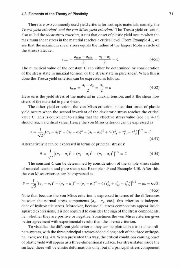
4.3 Elements of the Theory of Plasticity 71
There are two commonly used yield criteria for isotropic materials, namely, theTresca yield criterion6 and the von Mises yield criterion.7 The Tresca yield criterion,also called the shear stress criterion, states that onset of plastic yield occurs when themaximum shear stress in the material reaches a critical level. From Example 4.1, wesee that the maximum shear stress equals the radius of the largest Mohr’s circle ofthe stress state, i.e.,
τmax = σmax − σmin
2= σ1 − σ3
2= C (4-51)
The numerical value of the constant C can either be determined by considerationof the stress state in uniaxial tension, or the stress state in pure shear. When this isdone the Tresca yield criterion can be expressed as follows:
τmax = σ1 − σ3
2= σ0
2= k (4-52)
Here σ0 is the yield stress of the material in uniaxial tension, and k the shear flowstress of the material in pure shear.
The other yield criterion, the von Mises criterion, states that onset of plasticyield occurs when the second invariant of the deviatoric stress reaches the criticalvalue C. This is equivalent to stating that the effective stress value (see eq. 4-37)should reach a critical value. Hence the von Mises criterion can be expressed as
σ = 1√2
[(σx − σy)2 + (σy − σz)2 + (σz − σx)2 + 6
(τ 2
xy + τ 2yz + τ 2
xz
)]1/2 = C
(4-53)Alternatively it can be expressed in terms of principal stresses:
σ = 1√2
[(σ1 − σ2)2 + (σ2 − σ3)2 + (σ3 − σ1)2]1/2 = C (4-54)
The constant C can be determined by consideration of the simple stress statesof uniaxial tension and pure shear; see Example 4.9 and Example 4.10. After this,the von Mises criterion can be expressed as
σ = 1√2
[(σx − σy)2 + (σy − σz)
2 + (σz − σx)2 + 6(τ 2
xy + τ 2yz + τ 2
xz
)]1/2 = σ0 = k√
3
(4-55)Note that because the von Mises criterion is expressed in terms of the differencesbetween the normal stress components (σx − σy, etc.), this criterion is indepen-dent of hydrostatic stress. Moreover, because all stress components appear insidesquared expressions, it is not required to consider the sign of the stress components,i.e., whether they are positive or negative. Sometimes the von Mises criterion givesbetter agreement with experimental results than the Tresca criterion.
To visualize the different yield criteria, they can be plotted in a triaxial coordi-nate system, with the three principal stresses added along each of the three orthogo-nal axes; see Fig. 4.8. When presented this way, the critical conditions causing onsetof plastic yield will appear as a three-dimensional surface. For stress states inside thesurface, there will be elastic deformations only, but if a principal stress component
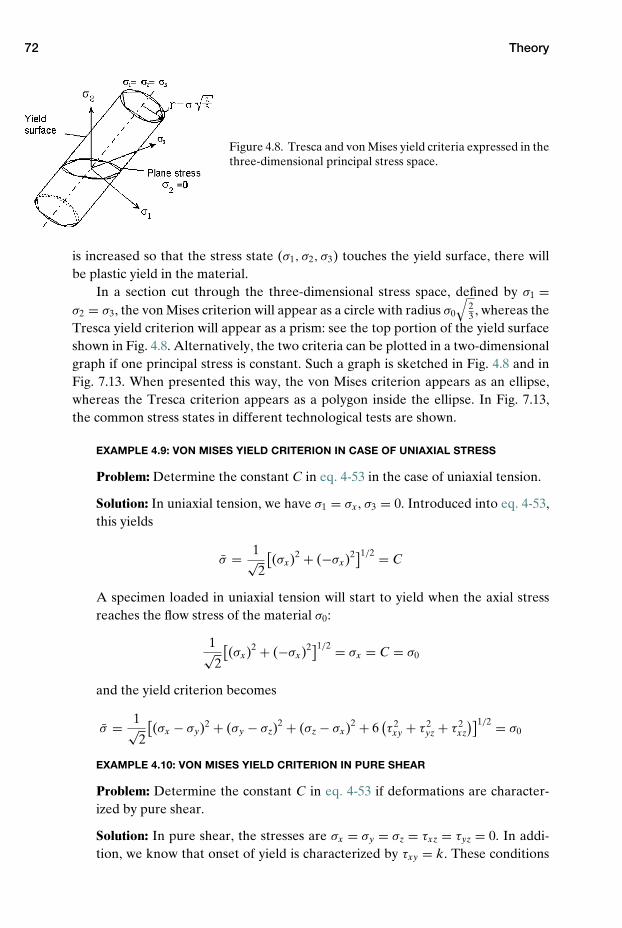
72 Theory
Figure 4.8. Tresca and von Mises yield criteria expressed in thethree-dimensional principal stress space.
is increased so that the stress state (σ1, σ2, σ3) touches the yield surface, there willbe plastic yield in the material.
In a section cut through the three-dimensional stress space, defined by σ1 =σ2 = σ3, the von Mises criterion will appear as a circle with radius σ0
√23 , whereas the
Tresca yield criterion will appear as a prism: see the top portion of the yield surfaceshown in Fig. 4.8. Alternatively, the two criteria can be plotted in a two-dimensionalgraph if one principal stress is constant. Such a graph is sketched in Fig. 4.8 and inFig. 7.13. When presented this way, the von Mises criterion appears as an ellipse,whereas the Tresca criterion appears as a polygon inside the ellipse. In Fig. 7.13,the common stress states in different technological tests are shown.
EXAMPLE 4.9: VON MISES YIELD CRITERION IN CASE OF UNIAXIAL STRESS
Problem: Determine the constant C in eq. 4-53 in the case of uniaxial tension.
Solution: In uniaxial tension, we have σ1 = σx, σ3 = 0. Introduced into eq. 4-53,this yields
σ = 1√2
[(σx)2 + (−σx)2]1/2 = C
A specimen loaded in uniaxial tension will start to yield when the axial stressreaches the flow stress of the material σ0:
1√2
[(σx)2 + (−σx)2]1/2 = σx = C = σ0
and the yield criterion becomes
σ = 1√2
[(σx − σy)2 + (σy − σz)
2 + (σz − σx)2 + 6(τ 2
xy + τ 2yz + τ 2
xz
)]1/2 = σ0
EXAMPLE 4.10: VON MISES YIELD CRITERION IN PURE SHEAR
Problem: Determine the constant C in eq. 4-53 if deformations are character-ized by pure shear.
Solution: In pure shear, the stresses are σx = σy = σz = τxz = τyz = 0. In addi-tion, we know that onset of yield is characterized by τxy = k. These conditions
4.3 Elements of the Theory of Plasticity 73
introduced into eq. 4-53 yield
σ = 1√2
[6τ 2
xy
]1/2 =√
3 · τxy =√
3 · k = C ⇒ C =√
3 · k
4.3.7 The Flow Rule
In the case of elastic deformation, Hooke’s law describes the relationship betweenstresses and strains. In the general stress state, the principal strain arising as a conse-quence of present stresses when determined by this law is given by the expression
e1 = 1E
[σ1 − ν(σ2 + σ3)] (4-56)
and corresponding expressions for the other principal elastic strains.In the case of plastic deformation, plastic strains are related to present stresses
in a similar way. The law that describes the relationship between stresses and strainsin the plastic state is commonly called the flow rule, or the Levy7–Mises8 flow rule,after the scientists who first proposed it. A common formulation of the flow rule is
dε1
σ ′1
= dε2
σ ′2
= dε3
σ ′3
= dλ (4-57)
or, alternatively,
dε1 = dε
σ
(σ1 − 1
2(σ2 + σ3)
)(4-58)
dε2 = dε
σ
(σ2 − 1
2(σ3 + σ1)
)(4-59)
dε3 = dε
σ
(σ3 − 1
2(σ1 + σ2)
)(4-60)
In this latter formulation, we see similarity with Hooke’s law: The constant ν inHooke’s law is replaced by 1
2 in the flow rule. In addition, the constant 1/E isreplaced by the ratio dε/σ , whose value changes as deformation proceeds. How-ever, this ratio is always positive, because the effective plastic strain incrementand the effective stress are always positive; see the definition of these parameters,eqs. 4-37–4-38.
EXAMPLE 4.11: LEVY–MISES FLOW RULE USED TO COMPUTE STRESSES IN PLANE
STRAIN COMPRESSION AND IN PLANE STRESS
Problem: A material with a constant flow stress σ0 is deformed up to a perma-nent plastic deformation εx in:
(i) plane compression with σ3 = 0,(ii) deformation with stress characterized by σx = σ1 = 2σ2 and σ3 = 0.
Determine the principal stresses in case (i) and the principal strains in case (ii).
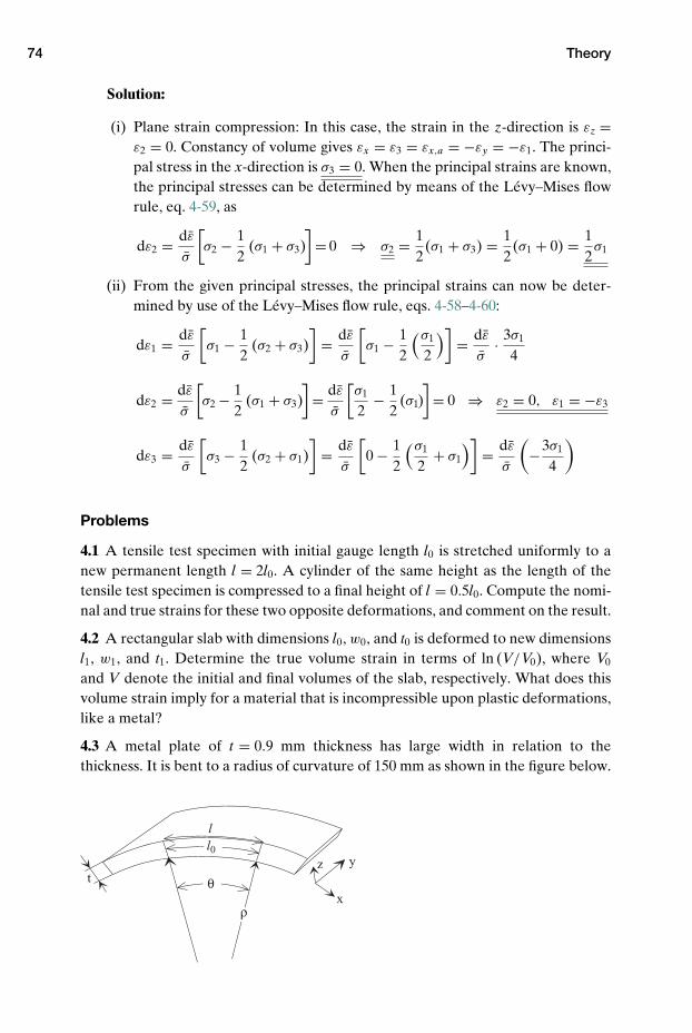
74 Theory
Solution:
(i) Plane strain compression: In this case, the strain in the z-direction is εz =ε2 = 0. Constancy of volume gives εx = ε3 = εx,a = −εy = −ε1. The princi-pal stress in the x-direction is σ3 = 0. When the principal strains are known,the principal stresses can be determined by means of the Levy–Mises flowrule, eq. 4-59, as
dε2 = dε
σ
[σ2 − 1
2(σ1 + σ3)
]= 0 ⇒ σ2 = 1
2(σ1 + σ3) = 1
2(σ1 + 0) = 1
2σ1
(ii) From the given principal stresses, the principal strains can now be deter-mined by use of the Levy–Mises flow rule, eqs. 4-58–4-60:
dε1 = dε
σ
[σ1 − 1
2(σ2 + σ3)
]= dε
σ
[σ1 − 1
2
(σ1
2
)]= dε
σ· 3σ1
4
dε2 = dε
σ
[σ2 − 1
2(σ1 + σ3)
]= dε
σ
[σ1
2− 1
2(σ1)
]= 0 ⇒ ε2 = 0, ε1 = −ε3
dε3 = dε
σ
[σ3 − 1
2(σ2 + σ1)
]= dε
σ
[0 − 1
2
(σ1
2+ σ1
)]= dε
σ
(−3σ1
4
)
Problems
4.1 A tensile test specimen with initial gauge length l0 is stretched uniformly to anew permanent length l = 2l0. A cylinder of the same height as the length of thetensile test specimen is compressed to a final height of l = 0.5l0. Compute the nomi-nal and true strains for these two opposite deformations, and comment on the result.
4.2 A rectangular slab with dimensions l0, w0, and t0 is deformed to new dimensionsl1, w1, and t1. Determine the true volume strain in terms of ln (V/V0), where V0
and V denote the initial and final volumes of the slab, respectively. What does thisvolume strain imply for a material that is incompressible upon plastic deformations,like a metal?
4.3 A metal plate of t = 0.9 mm thickness has large width in relation to thethickness. It is bent to a radius of curvature of 150 mm as shown in the figure below.
ρ
θ
l0
l
tz y
x
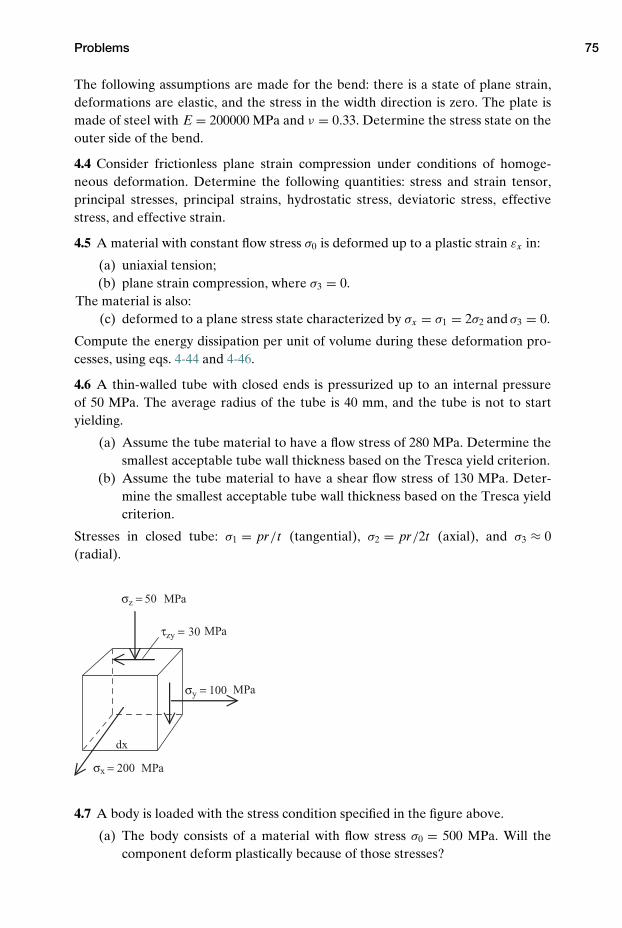
Problems 75
The following assumptions are made for the bend: there is a state of plane strain,deformations are elastic, and the stress in the width direction is zero. The plate ismade of steel with E = 200000 MPa and ν = 0.33. Determine the stress state on theouter side of the bend.
4.4 Consider frictionless plane strain compression under conditions of homoge-neous deformation. Determine the following quantities: stress and strain tensor,principal stresses, principal strains, hydrostatic stress, deviatoric stress, effectivestress, and effective strain.
4.5 A material with constant flow stress σ0 is deformed up to a plastic strain εx in:
(a) uniaxial tension;(b) plane strain compression, where σ3 = 0.
The material is also:(c) deformed to a plane stress state characterized by σx = σ1 = 2σ2 and σ3 = 0.
Compute the energy dissipation per unit of volume during these deformation pro-cesses, using eqs. 4-44 and 4-46.
4.6 A thin-walled tube with closed ends is pressurized up to an internal pressureof 50 MPa. The average radius of the tube is 40 mm, and the tube is not to startyielding.
(a) Assume the tube material to have a flow stress of 280 MPa. Determine thesmallest acceptable tube wall thickness based on the Tresca yield criterion.
(b) Assume the tube material to have a shear flow stress of 130 MPa. Deter-mine the smallest acceptable tube wall thickness based on the Tresca yieldcriterion.
Stresses in closed tube: σ1 = pr/t (tangential), σ2 = pr/2t (axial), and σ3 ≈ 0(radial).
σz = 50 MPa
MPa
dx
σy = 100 MPa
σx = 200 MPa
4.7 A body is loaded with the stress condition specified in the figure above.
(a) The body consists of a material with flow stress σ0 = 500 MPa. Will thecomponent deform plastically because of those stresses?
76 Theory
(b) Assume all stress components to be maintained, except for the stress in thex-direction, which is varied. Calculate the level of this stress componentupon onset of yielding of the material.
4.8 Consider that a circle grid analysis has been performed on a piece of sheet metalas described in Example 4.7. Determine the stress ratio σ1/σ during the formingoperation at the location of the deforming circle. Assume that the z-axis points inthe thickness direction of the plate and that there is plane stress characterized byσz = τyz = τzx = 0. Assume also the ratio α = σ2/σ1 to remain constant during thetest.
4.9 Show the validity of eq. 4-57, i.e., the flow rule, in the case of uniaxial tension.
4.10 The geometry of a thin-walled Al tube is characterized by a ratio r/t = 20,where r is the radius and t the thickness of the tube. Assume that the tube is closedat the ends and is pressurized up to the inner pressure p = 6.9 MPa, where it yieldsplastically. What will be the plastic strain in the tube in the tangential direction, i.e.,along its circumference, if one neglects elastic deformations? The flow curve of thematerial is given by σ (MPa) = 172.4(ε)0.25. The required formulas for the principalstresses are given in Problem 4.6.
NOTES
1. Hosford, W. F., and Caddell, R. M.: “Metal Forming, Mechanics and Metallurgy,” Cam-bridge Univ. Press, 2007.
2. Dieter, G.: “Mechanical Metallurgy,” McGraw-Hill, 1989.3. Chakrabarty, J.: “Theory of Plasticity,” Elsevier, 2006.4. Mohr, O.: “Zivilingeneur,” 1882, p. 113.5. Coffin, L. F., and Rogers, H. C.: Trans. Am. Soc. Metallurgists, Vol. 60, 1967, p. 681.6. Tresca, H.: “On the flow of solid bodies subjected to high pressures,” C. R. Acad. Sci.
Paris, Vol. 59, 1864, p. 754.7. Levy, M.: “Memoire sur les equations generales des mouvements interieurs des corps
solides, ductiles au-dela des limites ou l’elasticite pourrait les ramener a leur premieretat,” C. R. Acad. Sci. Paris, Vol. 70, 1870, p. 1323.
8. Mises, R.: “Mechanik der fasten Korper im plastisch deformablen Zustand,” GottingenNachrichten, Math. Phys. Kl., 1913, p. 582.
REFERENCES
Chakrabarty, J.: “Applied Plasticity,” Springer-Verlag, 2000.Rees, D. W. A.: “Basic Engineering Plasticity,” Elsevier, 2006.
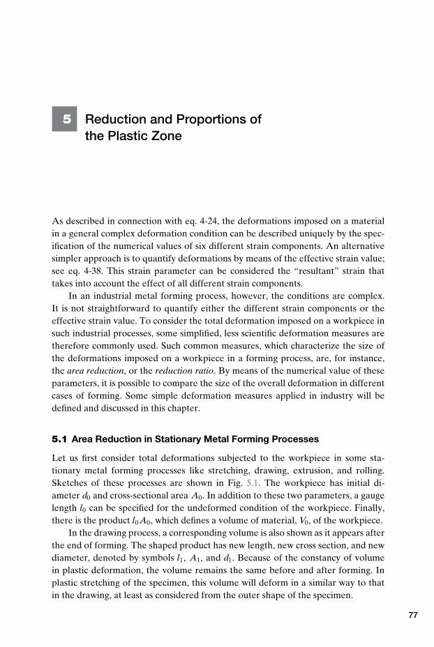
5 Reduction and Proportions ofthe Plastic Zone
As described in connection with eq. 4-24, the deformations imposed on a materialin a general complex deformation condition can be described uniquely by the spec-ification of the numerical values of six different strain components. An alternativesimpler approach is to quantify deformations by means of the effective strain value;see eq. 4-38. This strain parameter can be considered the “resultant” strain thattakes into account the effect of all different strain components.
In an industrial metal forming process, however, the conditions are complex.It is not straightforward to quantify either the different strain components or theeffective strain value. To consider the total deformation imposed on a workpiece insuch industrial processes, some simplified, less scientific deformation measures aretherefore commonly used. Such common measures, which characterize the size ofthe deformations imposed on a workpiece in a forming process, are, for instance,the area reduction, or the reduction ratio. By means of the numerical value of theseparameters, it is possible to compare the size of the overall deformation in differentcases of forming. Some simple deformation measures applied in industry will bedefined and discussed in this chapter.
5.1 Area Reduction in Stationary Metal Forming Processes
Let us first consider total deformations subjected to the workpiece in some sta-tionary metal forming processes like stretching, drawing, extrusion, and rolling.Sketches of these processes are shown in Fig. 5.1. The workpiece has initial di-ameter d0 and cross-sectional area A0. In addition to these two parameters, a gaugelength l0 can be specified for the undeformed condition of the workpiece. Finally,there is the product l0 A0, which defines a volume of material, V0, of the workpiece.
In the drawing process, a corresponding volume is also shown as it appears afterthe end of forming. The shaped product has new length, new cross section, and newdiameter, denoted by symbols l1, A1, and d1. Because of the constancy of volumein plastic deformation, the volume remains the same before and after forming. Inplastic stretching of the specimen, this volume will deform in a similar way to thatin the drawing, at least as considered from the outer shape of the specimen.
77
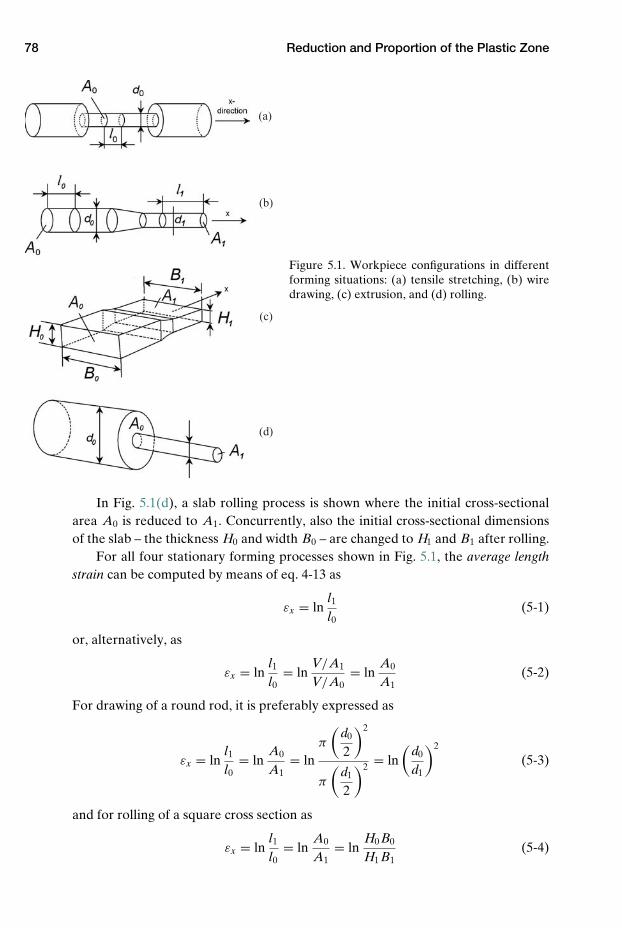
78 Reduction and Proportion of the Plastic Zone
(a)
(b)
(c)
(d)
Figure 5.1. Workpiece configurations in differentforming situations: (a) tensile stretching, (b) wiredrawing, (c) extrusion, and (d) rolling.
In Fig. 5.1(d), a slab rolling process is shown where the initial cross-sectionalarea A0 is reduced to A1. Concurrently, also the initial cross-sectional dimensionsof the slab – the thickness H0 and width B0 – are changed to H1 and B1 after rolling.
For all four stationary forming processes shown in Fig. 5.1, the average lengthstrain can be computed by means of eq. 4-13 as
εx = lnl1
l0(5-1)
or, alternatively, as
εx = lnl1
l0= ln
V/A1
V/A0= ln
A0
A1(5-2)
For drawing of a round rod, it is preferably expressed as
εx = lnl1
l0= ln
A0
A1= ln
π
(d0
2
)2
π
(d1
2
)2 = ln(
d0
d1
)2
(5-3)
and for rolling of a square cross section as
εx = lnl1
l0= ln
A0
A1= ln
H0 B0
H1 B1(5-4)
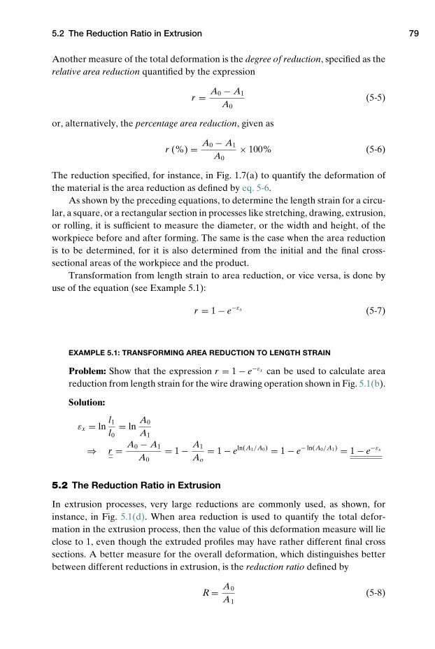
5.2 The Reduction Ratio in Extrusion 79
Another measure of the total deformation is the degree of reduction, specified as therelative area reduction quantified by the expression
r = A0 − A1
A0(5-5)
or, alternatively, the percentage area reduction, given as
r (%) = A0 − A1
A0× 100% (5-6)
The reduction specified, for instance, in Fig. 1.7(a) to quantify the deformation ofthe material is the area reduction as defined by eq. 5-6.
As shown by the preceding equations, to determine the length strain for a circu-lar, a square, or a rectangular section in processes like stretching, drawing, extrusion,or rolling, it is sufficient to measure the diameter, or the width and height, of theworkpiece before and after forming. The same is the case when the area reductionis to be determined, for it is also determined from the initial and the final cross-sectional areas of the workpiece and the product.
Transformation from length strain to area reduction, or vice versa, is done byuse of the equation (see Example 5.1):
r = 1 − e−εx (5-7)
EXAMPLE 5.1: TRANSFORMING AREA REDUCTION TO LENGTH STRAIN
Problem: Show that the expression r = 1 − e−εx can be used to calculate areareduction from length strain for the wire drawing operation shown in Fig. 5.1(b).
Solution:
εx = lnl1
l0= ln
A0
A1
⇒ r = A0 − A1
A0= 1 − A1
Ao= 1 − eln(A1/A0) = 1 − e− ln(A0/A1) = 1 − e−εx
5.2 The Reduction Ratio in Extrusion
In extrusion processes, very large reductions are commonly used, as shown, forinstance, in Fig. 5.1(d). When area reduction is used to quantify the total defor-mation in the extrusion process, then the value of this deformation measure will lieclose to 1, even though the extruded profiles may have rather different final crosssections. A better measure for the overall deformation, which distinguishes betterbetween different reductions in extrusion, is the reduction ratio defined by
R = A0
A1(5-8)
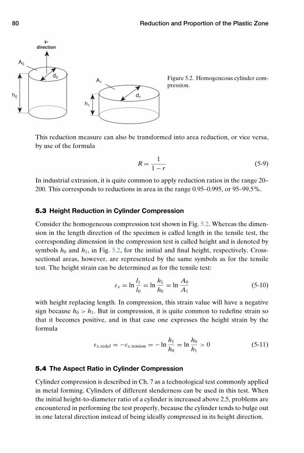
80 Reduction and Proportion of the Plastic Zone
x- direction
A0
h1
A1
h0
d0
d1
Figure 5.2. Homogeneous cylinder com-pression.
This reduction measure can also be transformed into area reduction, or vice versa,by use of the formula
R = 11 − r
(5-9)
In industrial extrusion, it is quite common to apply reduction ratios in the range 20–200. This corresponds to reductions in area in the range 0.95–0.995, or 95–99.5%.
5.3 Height Reduction in Cylinder Compression
Consider the homogeneous compression test shown in Fig. 5.2. Whereas the dimen-sion in the length direction of the specimen is called length in the tensile test, thecorresponding dimension in the compression test is called height and is denoted bysymbols h0 and h1, in Fig. 5.2, for the initial and final height, respectively. Cross-sectional areas, however, are represented by the same symbols as for the tensiletest. The height strain can be determined as for the tensile test:
εx = lnl1
l0= ln
h1
h0= ln
A0
A1(5-10)
with height replacing length. In compression, this strain value will have a negativesign because h0 > h1. But in compression, it is quite common to redefine strain sothat it becomes positive, and in that case one expresses the height strain by theformula
εx,redef = −εx,tension = − lnh1
h0= ln
h0
h1> 0 (5-11)
5.4 The Aspect Ratio in Cylinder Compression
Cylinder compression is described in Ch. 7 as a technological test commonly appliedin metal forming. Cylinders of different slenderness can be used in this test. Whenthe initial height-to-diameter ratio of a cylinder is increased above 2.5, problems areencountered in performing the test properly, because the cylinder tends to bulge outin one lateral direction instead of being ideally compressed in its height direction.
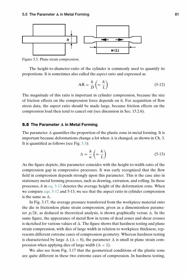
5.5 The Parameter � in Metal Forming 81
Figure 5.3. Plane strain compression.
The height-to-diameter-ratio of the cylinder is commonly used to quantify itsproportions. It is sometimes also called the aspect ratio and expressed as
AR = hD
(= h
L
)(5-12)
The magnitude of this ratio is important in cylinder compression, because the sizeof friction effects on the compression force depends on it. For acquisition of flowstress data, the aspect ratio should be made large, because friction effects on thecompression load then tend to cancel out (see discussion in Sec. 15.2.6).
5.5 The Parameter � in Metal Forming
The parameter � quantifies the proportion of the plastic zone in metal forming. It isimportant because deformations change a lot when � is changed, as shown in Ch. 3.It is quantified as follows (see Fig. 5.3):
� = hw
(= h
L
)(5-13)
As the figure depicts, this parameter coincides with the height-to-width ratio of thecompression gap in compressive processes. It was early recognized that the flowfield in compression depends strongly upon this parameter. This is the case also instationary metal forming processes, such as drawing, extrusion, and rolling. In theseprocesses, h in eq. 5-13 denotes the average height of the deformation zone. Whenwe compare eqs. 5-12 and 5-13, we see that the aspect ratio in cylinder compressionis the same as �.
In Fig. 3.17, the average pressure transferred from the workpiece material ontothe die in frictionless plane strain compression, given as a dimensionless parame-ter p/2k, as deduced in theoretical analysis, is shown graphically versus �. In thesame figure, the appearance of metal flow in terms of dead zones and shear crossesis sketched for various values of �. The figure shows that hardness testing and planestrain compression, with dies of large width in relation to workpiece thickness, rep-resents different extreme cases of compression geometry. Whereas hardness testingis characterized by large � (� > 8), the parameter � is small in plane strain com-pression when applying dies of large width (� < 1).
We also see from Fig. 3.17 that the geometrical conditions of the plastic zoneare quite different in these two extreme cases of compression. In hardness testing,
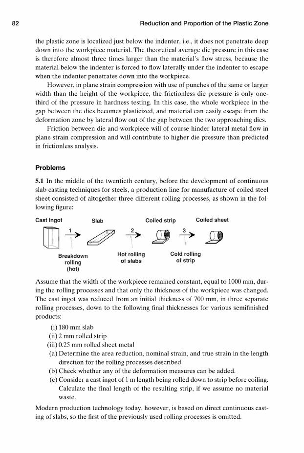
82 Reduction and Proportion of the Plastic Zone
the plastic zone is localized just below the indenter, i.e., it does not penetrate deepdown into the workpiece material. The theoretical average die pressure in this caseis therefore almost three times larger than the material’s flow stress, because thematerial below the indenter is forced to flow laterally under the indenter to escapewhen the indenter penetrates down into the workpiece.
However, in plane strain compression with use of punches of the same or largerwidth than the height of the workpiece, the frictionless die pressure is only one-third of the pressure in hardness testing. In this case, the whole workpiece in thegap between the dies becomes plasticized, and material can easily escape from thedeformation zone by lateral flow out of the gap between the two approaching dies.
Friction between die and workpiece will of course hinder lateral metal flow inplane strain compression and will contribute to higher die pressure than predictedin frictionless analysis.
Problems
5.1 In the middle of the twentieth century, before the development of continuousslab casting techniques for steels, a production line for manufacture of coiled steelsheet consisted of altogether three different rolling processes, as shown in the fol-lowing figure:
Cast ingot
Breakdown rolling (hot)
Slab
Hot rolling of slabs
Cold rolling of strip
Coiled strip Coiled sheet
1 2 3
Assume that the width of the workpiece remained constant, equal to 1000 mm, dur-ing the rolling processes and that only the thickness of the workpiece was changed.The cast ingot was reduced from an initial thickness of 700 mm, in three separaterolling processes, down to the following final thicknesses for various semifinishedproducts:
(i) 180 mm slab(ii) 2 mm rolled strip
(iii) 0.25 mm rolled sheet metal(a) Determine the area reduction, nominal strain, and true strain in the length
direction for the rolling processes described.(b) Check whether any of the deformation measures can be added.(c) Consider a cast ingot of 1 m length being rolled down to strip before coiling.
Calculate the final length of the resulting strip, if we assume no materialwaste.
Modern production technology today, however, is based on direct continuous cast-ing of slabs, so the first of the previously used rolling processes is omitted.

Problems 83
(d) Compute the total area reduction and the true strain in the length directionof the material, after the introduction of recent technology.
5.2 Calculate the area reduction and the nominal and true strains in the length direc-tion of the workpiece for the following cases:
(a) Cylinder compression characterized by h1 = 12 h0.
(b) Rolling step with rolling parameters B1 = B0 and H1 = 0.9H0.(c) Extrusion characterized by D0 = 100 mm and D1 = 10.2 mm.(d) Extrusion characterized by D0 = 100 mm and D1 = 8.0 mm.
On the basis of the computed deformations in (c) and (d), explain why it is practicalto use the reduction ratio to quantify overall deformations in extrusion.
5.3 Consider the FEM-simulated indirect Al extrusion process shown in Fig. 19.12,where a 95.7-mm-diameter billet is extruded down to a final rod of 28 mm diameter.In this case, a container of 100 mm diameter was used. Calculate the reduction ratioand the average length strain in this process. Discuss the obtained results in relationto the simulated effective strain distribution in the extruded rod (see Fig. 19.12).
5.4 Consider the FEM-simulated wiredrawing process shown in Fig. 23.19, where a3.43-mm-diameter wire was drawn down to a final dimension of 2.54 mm diameter.Calculate the reduction of area and the average length strain in this process. Discussthe obtained results in relation to the simulated effective strain distribution in thedrawn wire; see Fig. 23.19(a) and (b). Calculate also the parameter � in this case.
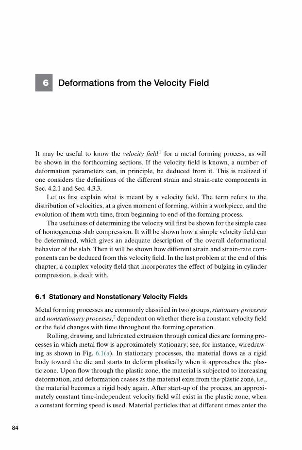
6 Deformations from the Velocity Field
It may be useful to know the velocity field 1 for a metal forming process, as willbe shown in the forthcoming sections. If the velocity field is known, a number ofdeformation parameters can, in principle, be deduced from it. This is realized ifone considers the definitions of the different strain and strain-rate components inSec. 4.2.1 and Sec. 4.3.3.
Let us first explain what is meant by a velocity field. The term refers to thedistribution of velocities, at a given moment of forming, within a workpiece, and theevolution of them with time, from beginning to end of the forming process.
The usefulness of determining the velocity will first be shown for the simple caseof homogeneous slab compression. It will be shown how a simple velocity field canbe determined, which gives an adequate description of the overall deformationalbehavior of the slab. Then it will be shown how different strain and strain-rate com-ponents can be deduced from this velocity field. In the last problem at the end of thischapter, a complex velocity field that incorporates the effect of bulging in cylindercompression, is dealt with.
6.1 Stationary and Nonstationary Velocity Fields
Metal forming processes are commonly classified in two groups, stationary processesand nonstationary processes,2 dependent on whether there is a constant velocity fieldor the field changes with time throughout the forming operation.
Rolling, drawing, and lubricated extrusion through conical dies are forming pro-cesses in which metal flow is approximately stationary; see, for instance, wiredraw-ing as shown in Fig. 6.1(a). In stationary processes, the material flows as a rigidbody toward the die and starts to deform plastically when it approaches the plas-tic zone. Upon flow through the plastic zone, the material is subjected to increasingdeformation, and deformation ceases as the material exits from the plastic zone, i.e.,the material becomes a rigid body again. After start-up of the process, an approxi-mately constant time-independent velocity field will exist in the plastic zone, whena constant forming speed is used. Material particles that at different times enter the
84
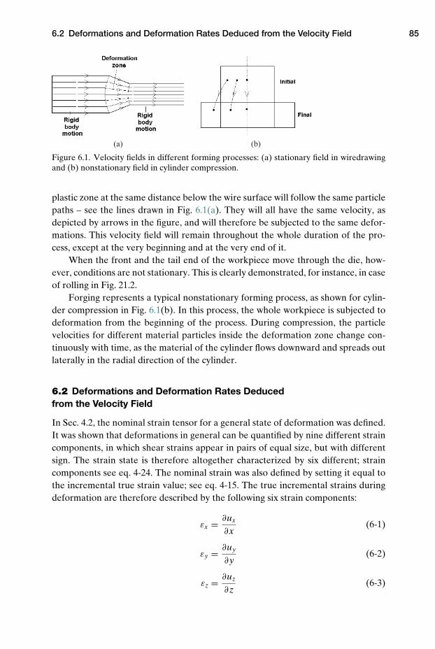
6.2 Deformations and Deformation Rates Deduced from the Velocity Field 85
(a) (b)
Figure 6.1. Velocity fields in different forming processes: (a) stationary field in wiredrawingand (b) nonstationary field in cylinder compression.
plastic zone at the same distance below the wire surface will follow the same particlepaths – see the lines drawn in Fig. 6.1(a). They will all have the same velocity, asdepicted by arrows in the figure, and will therefore be subjected to the same defor-mations. This velocity field will remain throughout the whole duration of the pro-cess, except at the very beginning and at the very end of it.
When the front and the tail end of the workpiece move through the die, how-ever, conditions are not stationary. This is clearly demonstrated, for instance, in caseof rolling in Fig. 21.2.
Forging represents a typical nonstationary forming process, as shown for cylin-der compression in Fig. 6.1(b). In this process, the whole workpiece is subjected todeformation from the beginning of the process. During compression, the particlevelocities for different material particles inside the deformation zone change con-tinuously with time, as the material of the cylinder flows downward and spreads outlaterally in the radial direction of the cylinder.
6.2 Deformations and Deformation Rates Deducedfrom the Velocity Field
In Sec. 4.2, the nominal strain tensor for a general state of deformation was defined.It was shown that deformations in general can be quantified by nine different straincomponents, in which shear strains appear in pairs of equal size, but with differentsign. The strain state is therefore altogether characterized by six different; straincomponents see eq. 4-24. The nominal strain was also defined by setting it equal tothe incremental true strain value; see eq. 4-15. The true incremental strains duringdeformation are therefore described by the following six strain components:
εx = ∂ux
∂x(6-1)
εy = ∂uy
∂y(6-2)
εz = ∂uz
∂z(6-3)
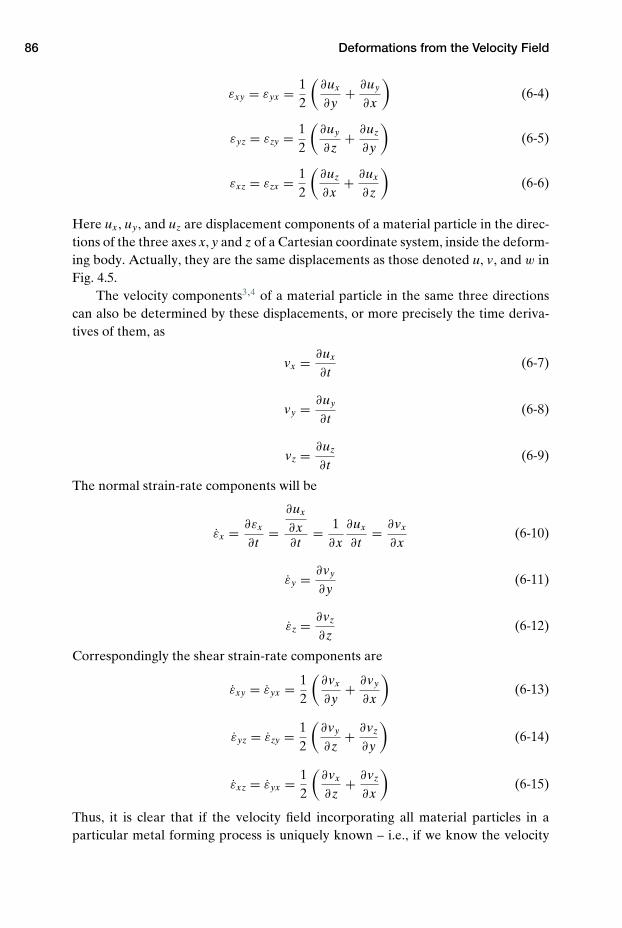
86 Deformations from the Velocity Field
εxy = εyx = 12
(∂ux
∂y+ ∂uy
∂x
)(6-4)
εyz = εzy = 12
(∂uy
∂z+ ∂uz
∂y
)(6-5)
εxz = εzx = 12
(∂uz
∂x+ ∂ux
∂z
)(6-6)
Here ux, uy, and uz are displacement components of a material particle in the direc-tions of the three axes x, y and z of a Cartesian coordinate system, inside the deform-ing body. Actually, they are the same displacements as those denoted u, v, and w inFig. 4.5.
The velocity components3,4 of a material particle in the same three directionscan also be determined by these displacements, or more precisely the time deriva-tives of them, as
vx = ∂ux
∂t(6-7)
vy = ∂uy
∂t(6-8)
vz = ∂uz
∂t(6-9)
The normal strain-rate components will be
εx = ∂εx
∂t=
∂ux
∂x∂t
= 1∂x
∂ux
∂t= ∂vx
∂x(6-10)
εy = ∂vy
∂y(6-11)
εz = ∂vz
∂z(6-12)
Correspondingly the shear strain-rate components are
εxy = εyx = 12
(∂vx
∂y+ ∂vy
∂x
)(6-13)
εyz = εzy = 12
(∂vy
∂z+ ∂vz
∂y
)(6-14)
εxz = εyx = 12
(∂vx
∂z+ ∂vz
∂x
)(6-15)
Thus, it is clear that if the velocity field incorporating all material particles in aparticular metal forming process is uniquely known – i.e., if we know the velocity
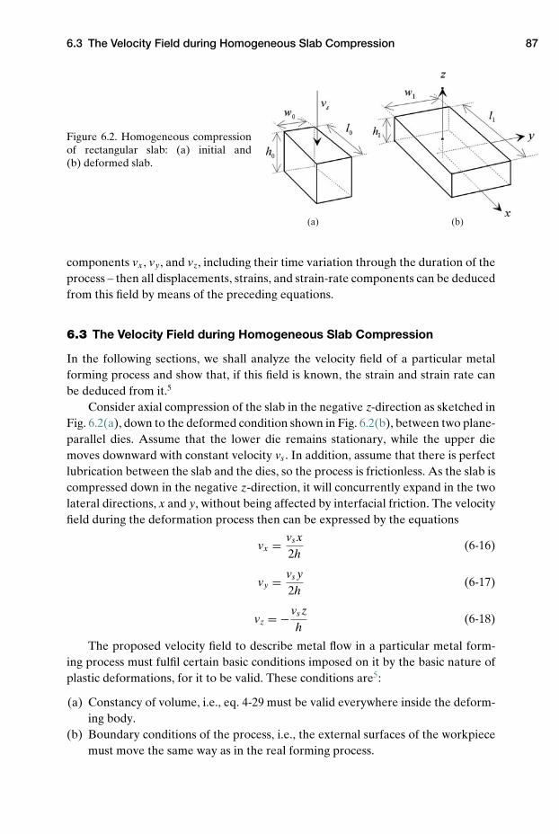
6.3 The Velocity Field during Homogeneous Slab Compression 87
(b)(a)
Figure 6.2. Homogeneous compressionof rectangular slab: (a) initial and(b) deformed slab.
components vx, vy, and vz, including their time variation through the duration of theprocess – then all displacements, strains, and strain-rate components can be deducedfrom this field by means of the preceding equations.
6.3 The Velocity Field during Homogeneous Slab Compression
In the following sections, we shall analyze the velocity field of a particular metalforming process and show that, if this field is known, the strain and strain rate canbe deduced from it.5
Consider axial compression of the slab in the negative z-direction as sketched inFig. 6.2(a), down to the deformed condition shown in Fig. 6.2(b), between two plane-parallel dies. Assume that the lower die remains stationary, while the upper diemoves downward with constant velocity vs . In addition, assume that there is perfectlubrication between the slab and the dies, so the process is frictionless. As the slab iscompressed down in the negative z-direction, it will concurrently expand in the twolateral directions, x and y, without being affected by interfacial friction. The velocityfield during the deformation process then can be expressed by the equations
vx = vs x2h
(6-16)
vy = vs y2h
(6-17)
vz = −vs zh
(6-18)
The proposed velocity field to describe metal flow in a particular metal form-ing process must fulfil certain basic conditions imposed on it by the basic nature ofplastic deformations, for it to be valid. These conditions are5:
(a) Constancy of volume, i.e., eq. 4-29 must be valid everywhere inside the deform-ing body.
(b) Boundary conditions of the process, i.e., the external surfaces of the workpiecemust move the same way as in the real forming process.
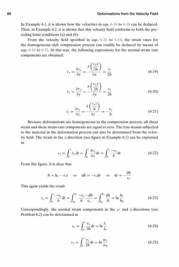
88 Deformations from the Velocity Field
In Example 6.1, it is shown how the velocities in eqs. 6-16 to 6-18 can be deduced.Then, in Example 6.2, it is shown that this velocity field conforms to both the pre-ceding basic conditions (a) and (b).
From the velocity field specified in eqs. 6-16 to 6-18, the strain rates forthe homogeneous slab compression process can readily be deduced by means ofeqs. 6-10 to 6-12. In this way, the following expressions for the normal strain ratecomponents are obtained:
εx = ∂vx
∂x=
∂
(vs x2h
)∂x
= vs
2h(6-19)
εy = ∂vy
∂y=
∂
(vs y2h
)∂y
= vs
2h(6-20)
εz = ∂vz
∂z=
∂
(vs zh
)∂z
= −vs
h(6-21)
Because deformations are homogeneous in the compression process, all shearstrain and shear strain-rate components are equal to zero. The true strains subjectedto the material in the deformation process can also be determined from the veloc-ity field. The strain in the z-direction (see figure in Example 6.1) can be expressedas
εz =∫ t
0εz dt =
∫ t
0
∂vz
∂zdt =
∫ t
0
−vs
hdt (6-22)
From this figure, it is clear that
h = h0 − vst ⇒ dh = −vsdt ⇒ dt = −dhvs
This again yields the result
εz =∫ t
0
−vs
hdt =
∫ h1
h0
−vs
h−dh
vs=
∫ h1
h0
dhh
= lnh1
h0(6-23)
Correspondingly, the normal strain components in the x- and y-directions (seeProblem 6.2) can be determined as
εx =∫ t
0
vs
2hdt = ln
l1
l0(6-24)
εy =∫ t
0
vs
2hdt = ln
w1
w0(6-25)
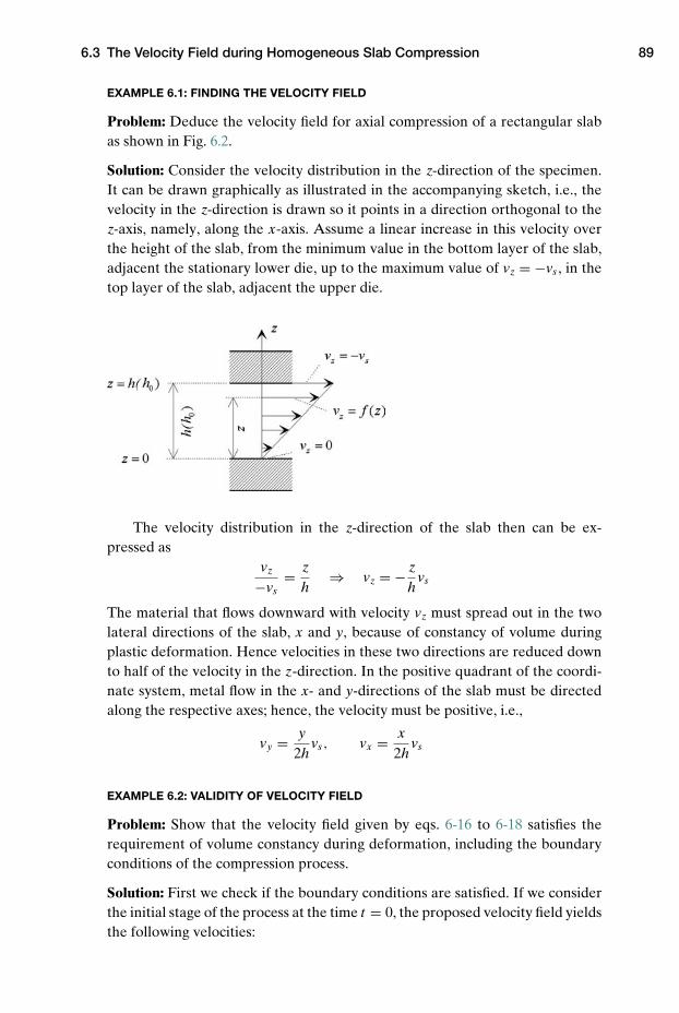
6.3 The Velocity Field during Homogeneous Slab Compression 89
EXAMPLE 6.1: FINDING THE VELOCITY FIELD
Problem: Deduce the velocity field for axial compression of a rectangular slabas shown in Fig. 6.2.
Solution: Consider the velocity distribution in the z-direction of the specimen.It can be drawn graphically as illustrated in the accompanying sketch, i.e., thevelocity in the z-direction is drawn so it points in a direction orthogonal to thez-axis, namely, along the x-axis. Assume a linear increase in this velocity overthe height of the slab, from the minimum value in the bottom layer of the slab,adjacent the stationary lower die, up to the maximum value of vz = −vs , in thetop layer of the slab, adjacent the upper die.
The velocity distribution in the z-direction of the slab then can be ex-pressed as
vz
−vs= z
h⇒ vz = − z
hvs
The material that flows downward with velocity vz must spread out in the twolateral directions of the slab, x and y, because of constancy of volume duringplastic deformation. Hence velocities in these two directions are reduced downto half of the velocity in the z-direction. In the positive quadrant of the coordi-nate system, metal flow in the x- and y-directions of the slab must be directedalong the respective axes; hence, the velocity must be positive, i.e.,
vy = y2h
vs, vx = x2h
vs
EXAMPLE 6.2: VALIDITY OF VELOCITY FIELD
Problem: Show that the velocity field given by eqs. 6-16 to 6-18 satisfies therequirement of volume constancy during deformation, including the boundaryconditions of the compression process.
Solution: First we check if the boundary conditions are satisfied. If we considerthe initial stage of the process at the time t = 0, the proposed velocity field yieldsthe following velocities:
90 Deformations from the Velocity Field
At the origin of the coordinate system: x = y = z = 0 ⇒ vx = vy = vz = 0.
On the moving surfaces of the slab (defined by x = l0/2, y = w0/2, and z = h0):
vx,surface = vsl0
4h0, vy,surface = vsw0
4h0, and vz,surface = −vs z
h0= −vsh0
h0= −vs
From this we see that the boundary conditions are fulfilled.Next we check whether the volume remains constant. The volume displaced
downward per unit of time by the upper die in the beginning of the compressionstroke equals vsw0l0. The corresponding volume per unit of time displaced inthe two lateral directions is
2vx,surface. h0w0 + 2vy,surface. l0h0 = 2vsl0
4h0h0w0 + 2
vsw0
4h0l0h0 = vsl0w0
Hence, constancy of volume is satisfied, for the volume displaced downwardequals the sum of the flow of volume in the two lateral directions.
Problems
6.1 Show that εx = (ln l1/l0) (eq. 6-24) during frictionless axial compression of aslab (Fig. 6.2), by deducing this normal strain from the material velocity in the x-direction, i.e., vx = vs x/2h.
6.2 A rectangular slab with initial height h0 = 10 mm is compressed axially withconstant compression velocity vs = 5 mm s−1. Assume frictionless conditions andhomogeneous deformations. Compute the strain-rate components and effectivestrain rate in the slab, both initially and after time t1 = 0.8 s. Compute the straincomponents and effective strain in the specimen at the same time.
6.3 The following velocity field6 has been proposed for the purpose of describingflow velocities in axisymmetric upsetting of a cylinder when there is friction so thatbulging occurs:
vθ = 0, vz = −2Az(1 − βz2/3), vr = Ar(1 − βz2/3)
Here β is a parameter representing the severity of the bulge, and A is determinedfrom the velocity boundary condition at z = h to be
A = VD
2h(1 − βh2
/3)
(a) Determine the general strain-rate tensor for this general case.(b) Find an expression for the effective strain-rate distribution inside the
cylinder.
NOTES
1. Altan, T., Oh, S. I., and Gegel, H. L.: “Metal Forming, Fundamentals and Applications,”ASM, 1983, pp. 41–44.
2. Lange, K.: “Handbook of Metal Forming,” McGraw-Hill, 1991, pp. 5.2–5.3.

Notes 91
3. Backofen, W. A.: “Deformation Processing,” Addison-Wesley, 1972.4. Rowe, G. W.: “Principles of Industrial Metalworking Processes,” Edward Arnold Pub-
lishers, London, 1977.5. Johnson, W., and Mellor, P. B.: “Engineering Plasticity,” Van Nostrand Reinhold,
London, 1975.6. Lee, C. H., and Altan, T.: “Influence of flow stress and friction upon metal flow in upset
forging of rings and cylinders,” ASME Trans. J. Engineering for Industry, Aug. 1972,p. 775.
7 Technological Tests and Physical Simulation
In order to model metal forming processes either by theoretical models or by FEMmodeling, as already shown in Ch. 3, it is required, for instance, to know the flowstress of the metal that is formed, and the actual friction between the die and theworkpiece. To obtain such data, a number of different test methods have been devel-oped over the years, by which it is possible to bring a specimen of the actual mate-rial, usually of small size, into a plastic state, and during plastic deformation of itmeasure the required deformation force, concurrently as the size of deformationssubjected to the specimen is measured. Tests of this kind are called technologicaltests and are commonly run on small specimens of the material, often in advancedequipment especially designed for the purpose. In this chapter, the most commontechnological tests for measurement of flow stress and ductility of metallic materialsare discussed. The main focus will be on the tensile test and the compression test.The basic mechanics of these technological tests, and how to determine stresses andstrains during the tests, will be reviewed.
7.1 Physical Simulation of Metal Forming
Some industrial metal forming processes – as for instance rolling, extrusion, andforging – are commonly run in large industrial equipment, where the possibilitiesof experimentation is limited. Most commonly the machinery lacks sensors to allowaccurate recording of relevant process parameters. Moreover, running of full-scaleexperiments in big industrial equipment is expensive. If there is continuous pro-duction in the equipment, full-scale experiments will reduce the productivity of theprocess to be investigated.
In heavy industrial equipment, large workpieces are shaped, and each specimentherefore will have high economic value. For example, if steel slabs of 5 ton weightare rolled, it is obvious that the loss of one slab will be expensive. If the product ismade with (for instance) wrong final dimensions or unacceptable mechanical prop-erties, it may have to be scrapped. Hence, industrial experimentation is limited byits cost, though recycling of metals by remelting and casting is common practice.
92
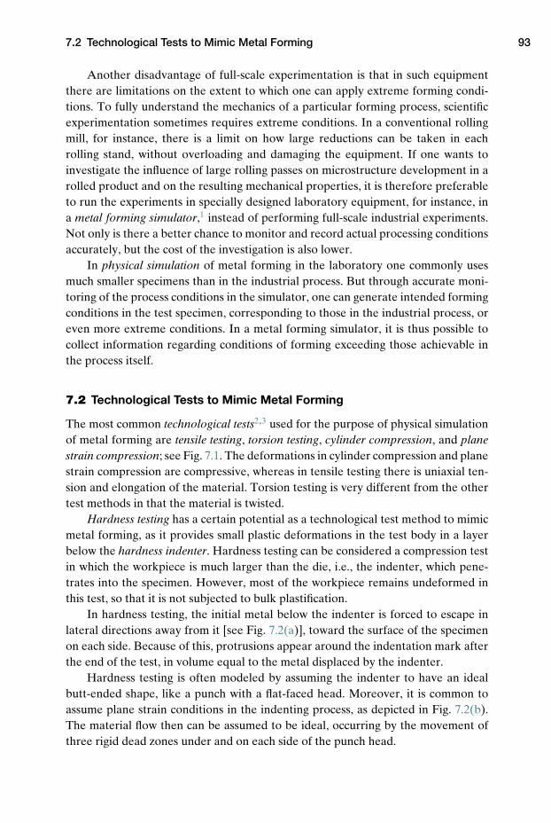
7.2 Technological Tests to Mimic Metal Forming 93
Another disadvantage of full-scale experimentation is that in such equipmentthere are limitations on the extent to which one can apply extreme forming condi-tions. To fully understand the mechanics of a particular forming process, scientificexperimentation sometimes requires extreme conditions. In a conventional rollingmill, for instance, there is a limit on how large reductions can be taken in eachrolling stand, without overloading and damaging the equipment. If one wants toinvestigate the influence of large rolling passes on microstructure development in arolled product and on the resulting mechanical properties, it is therefore preferableto run the experiments in specially designed laboratory equipment, for instance, ina metal forming simulator,1 instead of performing full-scale industrial experiments.Not only is there a better chance to monitor and record actual processing conditionsaccurately, but the cost of the investigation is also lower.
In physical simulation of metal forming in the laboratory one commonly usesmuch smaller specimens than in the industrial process. But through accurate moni-toring of the process conditions in the simulator, one can generate intended formingconditions in the test specimen, corresponding to those in the industrial process, oreven more extreme conditions. In a metal forming simulator, it is thus possible tocollect information regarding conditions of forming exceeding those achievable inthe process itself.
7.2 Technological Tests to Mimic Metal Forming
The most common technological tests2,3 used for the purpose of physical simulationof metal forming are tensile testing, torsion testing, cylinder compression, and planestrain compression; see Fig. 7.1. The deformations in cylinder compression and planestrain compression are compressive, whereas in tensile testing there is uniaxial ten-sion and elongation of the material. Torsion testing is very different from the othertest methods in that the material is twisted.
Hardness testing has a certain potential as a technological test method to mimicmetal forming, as it provides small plastic deformations in the test body in a layerbelow the hardness indenter. Hardness testing can be considered a compression testin which the workpiece is much larger than the die, i.e., the indenter, which pene-trates into the specimen. However, most of the workpiece remains undeformed inthis test, so that it is not subjected to bulk plastification.
In hardness testing, the initial metal below the indenter is forced to escape inlateral directions away from it [see Fig. 7.2(a)], toward the surface of the specimenon each side. Because of this, protrusions appear around the indentation mark afterthe end of the test, in volume equal to the metal displaced by the indenter.
Hardness testing is often modeled by assuming the indenter to have an idealbutt-ended shape, like a punch with a flat-faced head. Moreover, it is common toassume plane strain conditions in the indenting process, as depicted in Fig. 7.2(b).The material flow then can be assumed to be ideal, occurring by the movement ofthree rigid dead zones under and on each side of the punch head.
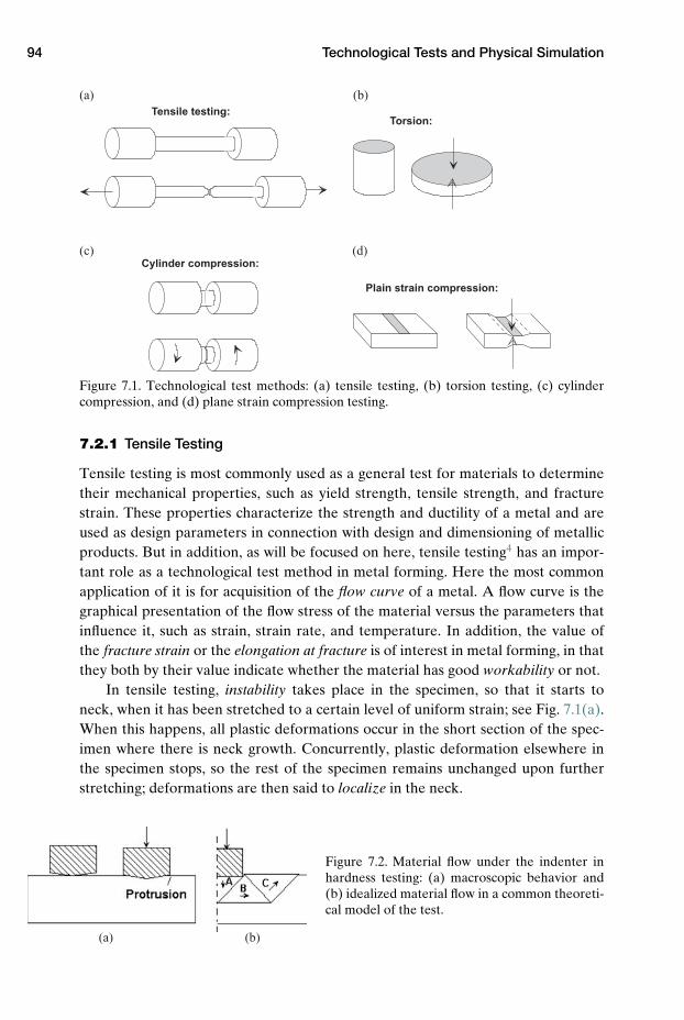
94 Technological Tests and Physical Simulation
Tensile testing:
Cylinder compression:
Torsion:
Plain strain compression:
(a)
(c) (d)
(b)
Figure 7.1. Technological test methods: (a) tensile testing, (b) torsion testing, (c) cylindercompression, and (d) plane strain compression testing.
7.2.1 Tensile Testing
Tensile testing is most commonly used as a general test for materials to determinetheir mechanical properties, such as yield strength, tensile strength, and fracturestrain. These properties characterize the strength and ductility of a metal and areused as design parameters in connection with design and dimensioning of metallicproducts. But in addition, as will be focused on here, tensile testing4 has an impor-tant role as a technological test method in metal forming. Here the most commonapplication of it is for acquisition of the flow curve of a metal. A flow curve is thegraphical presentation of the flow stress of the material versus the parameters thatinfluence it, such as strain, strain rate, and temperature. In addition, the value ofthe fracture strain or the elongation at fracture is of interest in metal forming, in thatthey both by their value indicate whether the material has good workability or not.
In tensile testing, instability takes place in the specimen, so that it starts toneck, when it has been stretched to a certain level of uniform strain; see Fig. 7.1(a).When this happens, all plastic deformations occur in the short section of the spec-imen where there is neck growth. Concurrently, plastic deformation elsewhere inthe specimen stops, so the rest of the specimen remains unchanged upon furtherstretching; deformations are then said to localize in the neck.
(a) (b)
Figure 7.2. Material flow under the indenter inhardness testing: (a) macroscopic behavior and(b) idealized material flow in a common theoreti-cal model of the test.
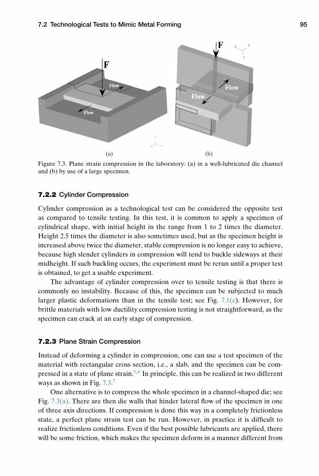
7.2 Technological Tests to Mimic Metal Forming 95
(a) (b)
Figure 7.3. Plane strain compression in the laboratory: (a) in a well-lubricated die channeland (b) by use of a large specimen.
7.2.2 Cylinder Compression
Cylinder compression as a technological test can be considered the opposite testas compared to tensile testing. In this test, it is common to apply a specimen ofcylindrical shape, with initial height in the range from 1 to 2 times the diameter.Height 2.5 times the diameter is also sometimes used, but as the specimen height isincreased above twice the diameter, stable compression is no longer easy to achieve,because high slender cylinders in compression will tend to buckle sideways at theirmidheight. If such buckling occurs, the experiment must be rerun until a proper testis obtained, to get a usable experiment.
The advantage of cylinder compression over to tensile testing is that there iscommonly no instability. Because of this, the specimen can be subjected to muchlarger plastic deformations than in the tensile test; see Fig. 7.1(c). However, forbrittle materials with low ductility compression testing is not straightforward, as thespecimen can crack at an early stage of compression.
7.2.3 Plane Strain Compression
Instead of deforming a cylinder in compression, one can use a test specimen of thematerial with rectangular cross section, i.e., a slab, and the specimen can be com-pressed in a state of plane strain.5,6 In principle, this can be realized in two differentways as shown in Fig. 7.3.7
One alternative is to compress the whole specimen in a channel-shaped die; seeFig. 7.3(a). There are then die walls that hinder lateral flow of the specimen in oneof three axis directions. If compression is done this way in a completely frictionlessstate, a perfect plane strain test can be run. However, in practice it is difficult torealize frictionless conditions. Even if the best possible lubricants are applied, therewill be some friction, which makes the specimen deform in a manner different from
96 Technological Tests and Physical Simulation
ideal plane strain. When this happens, the initially perfect rectangular cross sectionof the slab will not be rectangular after the test; hence, deformations will deviatefrom intended ones.
The simplest practical way to achieve close to plane strain conditions in com-pression, while the compression force is measured, is to compress a slab that onlypartly resides inside the compression gap; see Fig. 7.3(b). In this test, the rigid mate-rial outside the compression gap will hinder the metal inside the gap from flowing inthe lateral direction. Moreover, if a specimen with large breadth w (Fig. 7.12(a)) isused, the material in the middle of the specimen will deform under conditions closeto ideal plane strain.
7.2.4 Torsion
Torsion testing of metallic specimens is often used as an alternative method foracquisition of flow stress data and as an appropriate test for determination of theductility of a material. The torsion test2 is advantageous in some ways, one of thembeing that the test specimen can be subjected to large plastic deformations withoutsignificant shape change. However, because the specimen is twisted, the deforma-tions will be in shear. It is an interesting test method but will not be further dealtwith here, as it is considered beyond the scope of this book.
7.3 Physical Modeling of Metal Forming
Various kinds of commercial machines are available today that can impose defor-mation on metal specimens under controlled thermomechanical conditions cor-responding to metal forming. Generally, one can call these machines physicalsimulators. Such machines are able to deform metal specimens, under controlled,monitorable conditions, to mimic the deformation conditions in almost any metalforming process. Two machines of this kind will be described here, to illustrate theirworking principles and to show how such machines can be used for physical simula-tion of metal forming.
One simulator of this kind is the Gleeble machine,8 whose working principle isshown in Fig. 7.4. Gleeble machines are provided with different load capacities; forinstance, one particular model can deliver a maximum force of 50 tons (0.5 MN).With this load capacity, the machine can deform workpieces of metal under spec-ified, carefully monitored conditions. In a machine of this kind, only small work-pieces can be used if high compression speeds are to be achieved. The use of smallspecimens greatly limits the kinds of mechanical tests the deformed specimen can besubjected to after the technological test. Relevant tests on the material after techno-logical testing of a specimen of so small size are hardness testing and investigationof the microstructure by looking at sections cut through the material.
The Gleeble machine is built on a module principle, so that various exchange-able testing modules can be inserted to perform either tensile, compression, or tor-sion testing. When these tests are run on small specimens, miniature tensile test
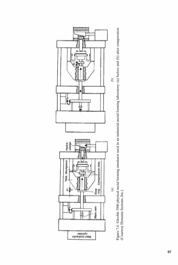
(a)
(b)
Fig
ure
7.4.
Gle
eble
3500
phys
ical
met
alfo
rmin
gsi
mul
ator
used
inan
indu
stri
alm
etal
form
ing
labo
rato
ry:(
a)be
fore
and
(b)
afte
rco
mpr
essi
on.
(Cou
rtes
yD
ynam
icSy
stem
s,In
c.)
97
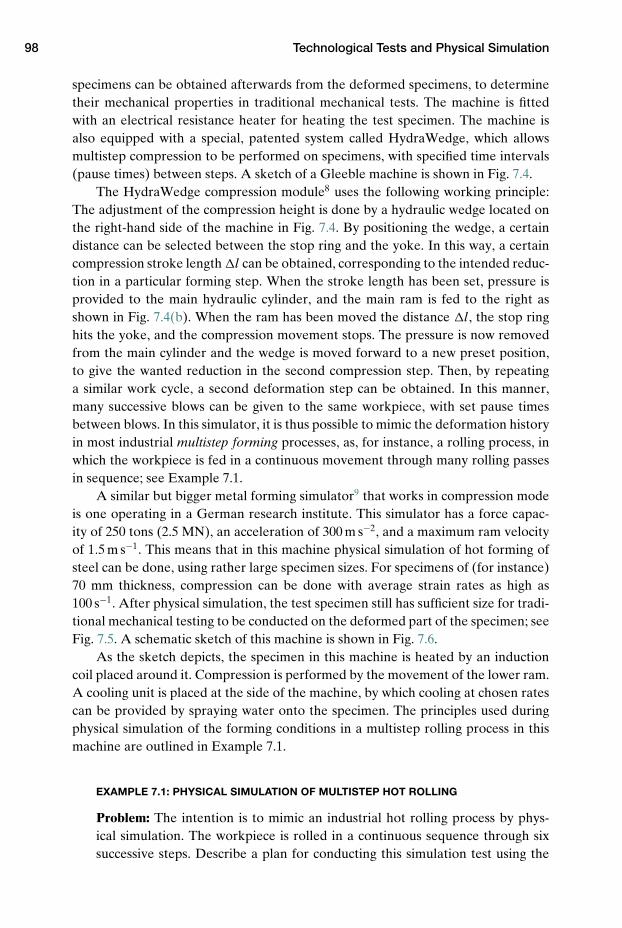
98 Technological Tests and Physical Simulation
specimens can be obtained afterwards from the deformed specimens, to determinetheir mechanical properties in traditional mechanical tests. The machine is fittedwith an electrical resistance heater for heating the test specimen. The machine isalso equipped with a special, patented system called HydraWedge, which allowsmultistep compression to be performed on specimens, with specified time intervals(pause times) between steps. A sketch of a Gleeble machine is shown in Fig. 7.4.
The HydraWedge compression module8 uses the following working principle:The adjustment of the compression height is done by a hydraulic wedge located onthe right-hand side of the machine in Fig. 7.4. By positioning the wedge, a certaindistance can be selected between the stop ring and the yoke. In this way, a certaincompression stroke length �l can be obtained, corresponding to the intended reduc-tion in a particular forming step. When the stroke length has been set, pressure isprovided to the main hydraulic cylinder, and the main ram is fed to the right asshown in Fig. 7.4(b). When the ram has been moved the distance �l, the stop ringhits the yoke, and the compression movement stops. The pressure is now removedfrom the main cylinder and the wedge is moved forward to a new preset position,to give the wanted reduction in the second compression step. Then, by repeatinga similar work cycle, a second deformation step can be obtained. In this manner,many successive blows can be given to the same workpiece, with set pause timesbetween blows. In this simulator, it is thus possible to mimic the deformation historyin most industrial multistep forming processes, as, for instance, a rolling process, inwhich the workpiece is fed in a continuous movement through many rolling passesin sequence; see Example 7.1.
A similar but bigger metal forming simulator9 that works in compression modeis one operating in a German research institute. This simulator has a force capac-ity of 250 tons (2.5 MN), an acceleration of 300 m s−2, and a maximum ram velocityof 1.5 m s−1. This means that in this machine physical simulation of hot forming ofsteel can be done, using rather large specimen sizes. For specimens of (for instance)70 mm thickness, compression can be done with average strain rates as high as100 s−1. After physical simulation, the test specimen still has sufficient size for tradi-tional mechanical testing to be conducted on the deformed part of the specimen; seeFig. 7.5. A schematic sketch of this machine is shown in Fig. 7.6.
As the sketch depicts, the specimen in this machine is heated by an inductioncoil placed around it. Compression is performed by the movement of the lower ram.A cooling unit is placed at the side of the machine, by which cooling at chosen ratescan be provided by spraying water onto the specimen. The principles used duringphysical simulation of the forming conditions in a multistep rolling process in thismachine are outlined in Example 7.1.
EXAMPLE 7.1: PHYSICAL SIMULATION OF MULTISTEP HOT ROLLING
Problem: The intention is to mimic an industrial hot rolling process by phys-ical simulation. The workpiece is rolled in a continuous sequence through sixsuccessive steps. Describe a plan for conducting this simulation test using the
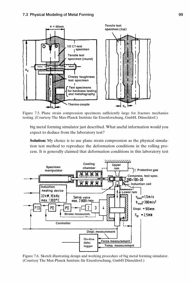
7.3 Physical Modeling of Metal Forming 99
Figure 7.5. Plane strain compression specimens sufficiently large for fracture mechanicstesting. (Courtesy The Max-Planck Institute fur Eisenforschung, GmbH, Dusseldorf.)
big metal forming simulator just described. What useful information would youexpect to deduce from the laboratory test?
Solution: My choice is to use plane strain compression as the physical simula-tion test method to reproduce the deformation conditions in the rolling pro-cess. It is generally claimed that deformation conditions in this laboratory test
Figure 7.6. Sketch illustrating design and working procedure of big metal forming simulator.(Courtesy The Max-Planck Institute fur Eisenforschung, GmbH Dusseldorf.)
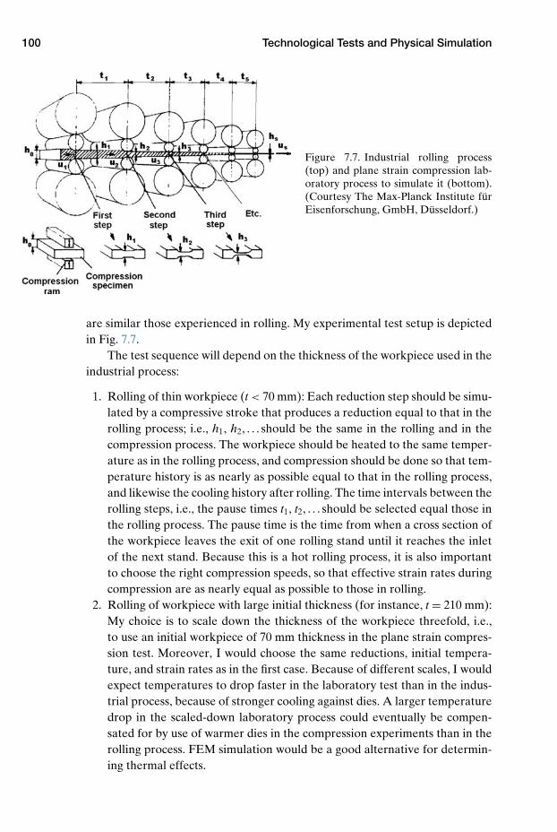
100 Technological Tests and Physical Simulation
Figure 7.7. Industrial rolling process(top) and plane strain compression lab-oratory process to simulate it (bottom).(Courtesy The Max-Planck Institute furEisenforschung, GmbH, Dusseldorf.)
are similar those experienced in rolling. My experimental test setup is depictedin Fig. 7.7.
The test sequence will depend on the thickness of the workpiece used in theindustrial process:
1. Rolling of thin workpiece (t < 70 mm): Each reduction step should be simu-lated by a compressive stroke that produces a reduction equal to that in therolling process; i.e., h1, h2, . . . should be the same in the rolling and in thecompression process. The workpiece should be heated to the same temper-ature as in the rolling process, and compression should be done so that tem-perature history is as nearly as possible equal to that in the rolling process,and likewise the cooling history after rolling. The time intervals between therolling steps, i.e., the pause times t1, t2, . . . should be selected equal those inthe rolling process. The pause time is the time from when a cross section ofthe workpiece leaves the exit of one rolling stand until it reaches the inletof the next stand. Because this is a hot rolling process, it is also importantto choose the right compression speeds, so that effective strain rates duringcompression are as nearly equal as possible to those in rolling.
2. Rolling of workpiece with large initial thickness (for instance, t = 210 mm):My choice is to scale down the thickness of the workpiece threefold, i.e.,to use an initial workpiece of 70 mm thickness in the plane strain compres-sion test. Moreover, I would choose the same reductions, initial tempera-ture, and strain rates as in the first case. Because of different scales, I wouldexpect temperatures to drop faster in the laboratory test than in the indus-trial process, because of stronger cooling against dies. A larger temperaturedrop in the scaled-down laboratory process could eventually be compen-sated for by use of warmer dies in the compression experiments than in therolling process. FEM simulation would be a good alternative for determin-ing thermal effects.
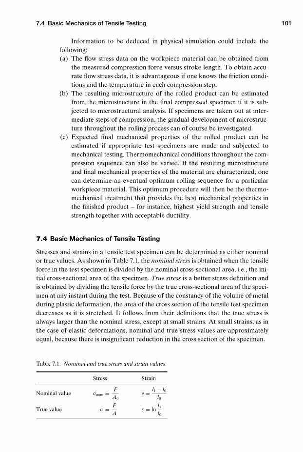
7.4 Basic Mechanics of Tensile Testing 101
Information to be deduced in physical simulation could include thefollowing:(a) The flow stress data on the workpiece material can be obtained from
the measured compression force versus stroke length. To obtain accu-rate flow stress data, it is advantageous if one knows the friction condi-tions and the temperature in each compression step.
(b) The resulting microstructure of the rolled product can be estimatedfrom the microstructure in the final compressed specimen if it is sub-jected to microstructural analysis. If specimens are taken out at inter-mediate steps of compression, the gradual development of microstruc-ture throughout the rolling process can of course be investigated.
(c) Expected final mechanical properties of the rolled product can beestimated if appropriate test specimens are made and subjected tomechanical testing. Thermomechanical conditions throughout the com-pression sequence can also be varied. If the resulting microstructureand final mechanical properties of the material are characterized, onecan determine an eventual optimum rolling sequence for a particularworkpiece material. This optimum procedure will then be the thermo-mechanical treatment that provides the best mechanical properties inthe finished product – for instance, highest yield strength and tensilestrength together with acceptable ductility.
7.4 Basic Mechanics of Tensile Testing
Stresses and strains in a tensile test specimen can be determined as either nominalor true values. As shown in Table 7.1, the nominal stress is obtained when the tensileforce in the test specimen is divided by the nominal cross-sectional area, i.e., the ini-tial cross-sectional area of the specimen. True stress is a better stress definition andis obtained by dividing the tensile force by the true cross-sectional area of the speci-men at any instant during the test. Because of the constancy of the volume of metalduring plastic deformation, the area of the cross section of the tensile test specimendecreases as it is stretched. It follows from their definitions that the true stress isalways larger than the nominal stress, except at small strains. At small strains, as inthe case of elastic deformations, nominal and true stress values are approximatelyequal, because there is insignificant reduction in the cross section of the specimen.
Table 7.1. Nominal and true stress and strain values
Stress Strain
Nominal value σnom = FA0
e = l1 − l0
l0
True value σ = FA
ε = lnl1
l0
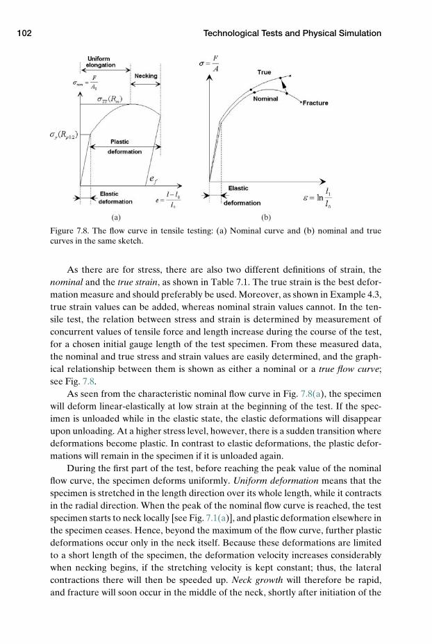
102 Technological Tests and Physical Simulation
(a) (b)
Figure 7.8. The flow curve in tensile testing: (a) Nominal curve and (b) nominal and truecurves in the same sketch.
As there are for stress, there are also two different definitions of strain, thenominal and the true strain, as shown in Table 7.1. The true strain is the best defor-mation measure and should preferably be used. Moreover, as shown in Example 4.3,true strain values can be added, whereas nominal strain values cannot. In the ten-sile test, the relation between stress and strain is determined by measurement ofconcurrent values of tensile force and length increase during the course of the test,for a chosen initial gauge length of the test specimen. From these measured data,the nominal and true stress and strain values are easily determined, and the graph-ical relationship between them is shown as either a nominal or a true flow curve;see Fig. 7.8.
As seen from the characteristic nominal flow curve in Fig. 7.8(a), the specimenwill deform linear-elastically at low strain at the beginning of the test. If the spec-imen is unloaded while in the elastic state, the elastic deformations will disappearupon unloading. At a higher stress level, however, there is a sudden transition wheredeformations become plastic. In contrast to elastic deformations, the plastic defor-mations will remain in the specimen if it is unloaded again.
During the first part of the test, before reaching the peak value of the nominalflow curve, the specimen deforms uniformly. Uniform deformation means that thespecimen is stretched in the length direction over its whole length, while it contractsin the radial direction. When the peak of the nominal flow curve is reached, the testspecimen starts to neck locally [see Fig. 7.1(a)], and plastic deformation elsewhere inthe specimen ceases. Hence, beyond the maximum of the flow curve, further plasticdeformations occur only in the neck itself. Because these deformations are limitedto a short length of the specimen, the deformation velocity increases considerablywhen necking begins, if the stretching velocity is kept constant; thus, the lateralcontractions there will then be speeded up. Neck growth will therefore be rapid,and fracture will soon occur in the middle of the neck, shortly after initiation of the
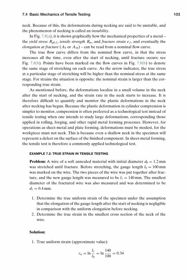
7.4 Basic Mechanics of Tensile Testing 103
neck. Because of this, the deformations during necking are said to be unstable, andthe phenomenon of necking is called an instability.
In Fig. 7.8(a), it is shown graphically how the mechanical properties of a metal –the yield stress Rp0,2, tensile strength Rm, and fracture strain e f , and eventually theelongation at fracture (A5 or A10) – can be read from a nominal flow curve.
The true flow curve differs from the nominal flow curve, in that the stressincreases all the time, even after the start of necking, until fracture occurs; seeFig. 7.8(b). Points have been marked on the flow curves in Fig. 7.8(b) to denotethe same stage of stretching on each curve. As the arrow indicates, the true stressat a particular stage of stretching will be higher than the nominal stress at the samestage. For strains the situation is opposite: the nominal strain is larger than the cor-responding true strain.
As mentioned before, the deformations localize in a small volume in the neckafter the start of necking, and the strain rate in the neck starts to increase. It istherefore difficult to quantify and monitor the plastic deformations in the neckafter necking has begun. Because the plastic deformation in cylinder compression issimpler to monitor, compression is often preferred as a technological test instead oftensile testing when one intends to study large deformations, corresponding thoseapplied in rolling, forging, and other rapid metal forming processes. However, foroperations as sheet-metal and plate forming, deformations must be modest, for theworkpiece must not neck. This is because even a shallow neck in the specimen willrepresent a defect on the surface of the finished component. In sheet-metal forming,the tensile test is therefore a commonly applied technological test.
EXAMPLE 7.2: TRUE STRAIN IN TENSILE TESTING
Problem: A wire of a soft annealed material with initial diameter d0 = 1.2 mmwas stretched until fracture. Before stretching, the gauge length l0 = 100 mmwas marked on the wire. The two pieces of the wire was put together after frac-ture, and the new gauge length was measured to be l1 = 140 mm. The smallestdiameter of the fractured wire was also measured and was determined to bed1 = 0.4 mm.
1. Determine the true uniform strain of the specimen under the assumptionthat the elongation of the gauge length after the start of necking is negligiblein comparison with the uniform elongation before necking.
2. Determine the true strain in the smallest cross section of the neck of thewire.
Solution:
1. True uniform strain (approximate value):
εu = lnl1
l0= ln
140100
= 0.34
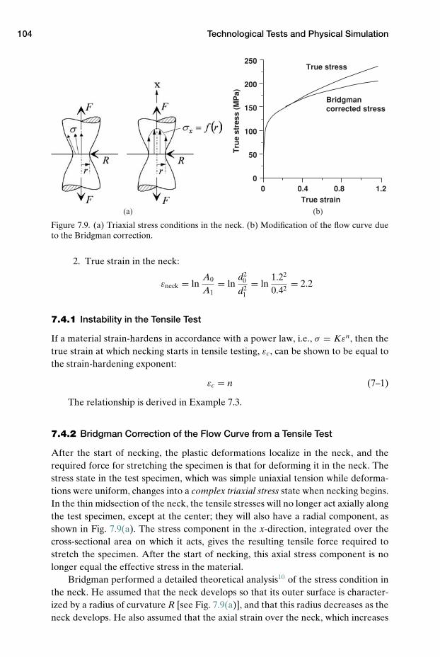
104 Technological Tests and Physical Simulation
(a) (b)
250
200
150
100
50
00 0.4 0.8 1.2
True strain
Bridgman corrected stress
True stress
Tru
e st
ress
(M
Pa)
Figure 7.9. (a) Triaxial stress conditions in the neck. (b) Modification of the flow curve dueto the Bridgman correction.
2. True strain in the neck:
εneck = lnA0
A1= ln
d20
d21
= ln1.22
0.42= 2.2
7.4.1 Instability in the Tensile Test
If a material strain-hardens in accordance with a power law, i.e., σ = Kεn, then thetrue strain at which necking starts in tensile testing, εc, can be shown to be equal tothe strain-hardening exponent:
εc = n (7–1)
The relationship is derived in Example 7.3.
7.4.2 Bridgman Correction of the Flow Curve from a Tensile Test
After the start of necking, the plastic deformations localize in the neck, and therequired force for stretching the specimen is that for deforming it in the neck. Thestress state in the test specimen, which was simple uniaxial tension while deforma-tions were uniform, changes into a complex triaxial stress state when necking begins.In the thin midsection of the neck, the tensile stresses will no longer act axially alongthe test specimen, except at the center; they will also have a radial component, asshown in Fig. 7.9(a). The stress component in the x-direction, integrated over thecross-sectional area on which it acts, gives the resulting tensile force required tostretch the specimen. After the start of necking, this axial stress component is nolonger equal the effective stress in the material.
Bridgman performed a detailed theoretical analysis10 of the stress condition inthe neck. He assumed that the neck develops so that its outer surface is character-ized by a radius of curvature R [see Fig. 7.9(a)], and that this radius decreases as theneck develops. He also assumed that the axial strain over the neck, which increases
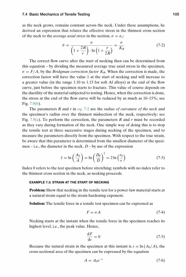
7.4 Basic Mechanics of Tensile Testing 105
as the neck grows, remains constant across the neck. Under these assumptions, hederived an expression that relates the effective stress in the thinnest cross sectionof the neck to the average axial stress in the section, σ = σx:
σ = σ(1 + 2R
r
)· ln
(1 + r
2R
) = σ
KB(7-2)
The correct flow curve after the start of necking then can be determined fromthis equation – by dividing the measured average true axial stress in the specimen,σ = F/A, by the Bridgman correction factor KB. When the correction is made, thecorrection factor will have the value 1 at the start of necking and will increase toa greater value (in the range 1.10 to 1.15 for soft Al alloys) at the end of the flowcurve, just before the specimen starts to fracture. This value of course depends onthe ductility of the material subjected to testing. Hence, when the correction is done,the stress at the end of the flow curve will be reduced by as much as 10–15%; seeFig. 7.9(b).
The parameters R and r in eq. 7-2 are the radius of curvature of the neck andthe specimen’s radius over the thinnest midsection of the neck, respectively; seeFig. 7.9(a). To perform the correction, the parameters R and r must be recordedas they vary during formation of the neck. One simple way of doing this is to stopthe tensile test at three successive stages during necking of the specimen, and tomeasure the parameters directly from the specimen. With respect to the true strain,be aware that this parameter is determined from the smallest diameter of the speci-men – i.e., the diameter in the neck, D – by use of the expression
ε = ln(
A0
A
)= ln
(D0
D
)2
= 2 ln(r0
r
)(7-3)
Index 0 refers to the test specimen before stretching; symbols with no index refer tothe thinnest cross section in the neck, as necking proceeds.
EXAMPLE 7.3: STRAIN AT THE START OF NECKING
Problem: Show that necking in the tensile test for a power-law material starts ata natural strain equal to the strain hardening exponent.
Solution: The tensile force in a tensile test specimen can be expressed as
F = σ A (7-4)
Necking starts at the instant when the tensile force in the specimen reaches itshighest level, i.e., the peak value. Hence,
dFdε
= 0 (7-5)
Because the natural strain in the specimen at this instant is ε = ln (A0/A), thecross-sectional area of the specimen can be expressed by the equation
A = A0e−ε (7-6)
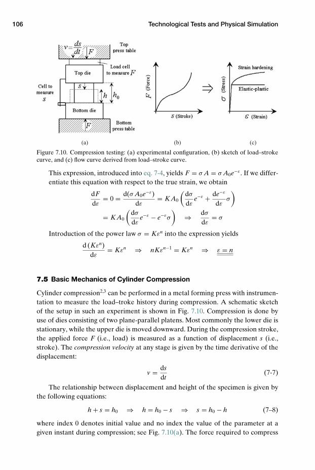
106 Technological Tests and Physical Simulation
(a) (b) (c)
Figure 7.10. Compression testing: (a) experimental configuration, (b) sketch of load–strokecurve, and (c) flow curve derived from load–stroke curve.
This expression, introduced into eq. 7-4, yields F = σ A = σ A0e−ε. If we differ-entiate this equation with respect to the true strain, we obtain
dFdε
= 0 = d(σ A0e−ε)dε
= K A0
(dσ
dεe−ε + de−ε
dεσ
)
= K A0
(dσ
dεe−ε − e−εσ
)⇒ dσ
dε= σ
Introduction of the power law σ = Kεn into the expression yields
d (Kεn)dε
= Kεn ⇒ nKεn−1 = Kεn ⇒ ε = n
7.5 Basic Mechanics of Cylinder Compression
Cylinder compression2,3 can be performed in a metal forming press with instrumen-tation to measure the load–troke history during compression. A schematic sketchof the setup in such an experiment is shown in Fig. 7.10. Compression is done byuse of dies consisting of two plane-parallel platens. Most commonly the lower die isstationary, while the upper die is moved downward. During the compression stroke,the applied force F (i.e., load) is measured as a function of displacement s (i.e.,stroke). The compression velocity at any stage is given by the time derivative of thedisplacement:
v = dsdt
(7-7)
The relationship between displacement and height of the specimen is given bythe following equations:
h + s = h0 ⇒ h = h0 − s ⇒ s = h0 − h (7–8)
where index 0 denotes initial value and no index the value of the parameter at agiven instant during compression; see Fig. 7.10(a). The force required to compress
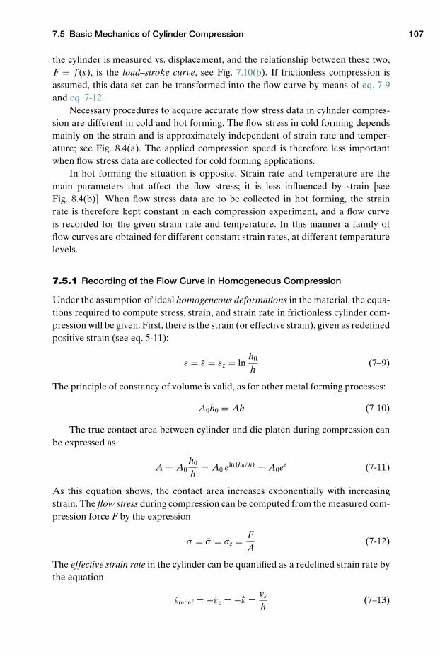
7.5 Basic Mechanics of Cylinder Compression 107
the cylinder is measured vs. displacement, and the relationship between these two,F = f (s), is the load–stroke curve, see Fig. 7.10(b). If frictionless compression isassumed, this data set can be transformed into the flow curve by means of eq. 7-9and eq. 7-12.
Necessary procedures to acquire accurate flow stress data in cylinder compres-sion are different in cold and hot forming. The flow stress in cold forming dependsmainly on the strain and is approximately independent of strain rate and temper-ature; see Fig. 8.4(a). The applied compression speed is therefore less importantwhen flow stress data are collected for cold forming applications.
In hot forming the situation is opposite. Strain rate and temperature are themain parameters that affect the flow stress; it is less influenced by strain [seeFig. 8.4(b)]. When flow stress data are to be collected in hot forming, the strainrate is therefore kept constant in each compression experiment, and a flow curveis recorded for the given strain rate and temperature. In this manner a family offlow curves are obtained for different constant strain rates, at different temperaturelevels.
7.5.1 Recording of the Flow Curve in Homogeneous Compression
Under the assumption of ideal homogeneous deformations in the material, the equa-tions required to compute stress, strain, and strain rate in frictionless cylinder com-pression will be given. First, there is the strain (or effective strain), given as redefinedpositive strain (see eq. 5-11):
ε = ε = εz = lnh0
h(7–9)
The principle of constancy of volume is valid, as for other metal forming processes:
A0h0 = Ah (7-10)
The true contact area between cylinder and die platen during compression canbe expressed as
A = A0h0
h= A0 eln (h0/h) = A0eε (7-11)
As this equation shows, the contact area increases exponentially with increasingstrain. The flow stress during compression can be computed from the measured com-pression force F by the expression
σ = σ = σz = FA
(7-12)
The effective strain rate in the cylinder can be quantified as a redefined strain rate bythe equation
εredef = −εz = − ˙ε = vs
h(7–13)
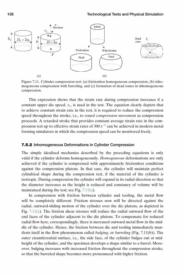
108 Technological Tests and Physical Simulation
(a) (b)
Figure 7.11. Cylinder compression test: (a) frictionless homogeneous compression, (b) inho-mogeneous compression with barreling, and (c) formation of dead zones in inhomogeneouscompression.
This expression shows that the strain rate during compression increases if aconstant upper die speed, vs , is used in the test. The equation clearly depicts thatto achieve constant strain rate in the test, it is required to reduce the compressionspeed throughout the stroke, i.e., to retard compression movement as compressionproceeds. A retarded stroke that provides constant average strain rate in the com-pression test up to effective strain rates of 300 s−1 can be achieved in modern metalforming simulators in which the compression speed can be monitored freely.
7.5.2 Inhomogeneous Deformations in Cylinder Compression
The simple idealized mechanics described by the preceding equations is onlyvalid if the cylinder deforms homogeneously. Homogeneous deformations are onlyachieved if the cylinder is compressed with approximately frictionless conditionsagainst the compression platens. In that case, the cylinder will maintain perfectcylindrical shape during the compression test, if the material of the cylinder isisotropic. During compression the cylinder will expand in its radial direction so thatthe diameter increases as the height is reduced and constancy of volume will bemaintained during the test; see Fig. 7.11(a).
In compression with friction between cylinder and tooling, the metal flowwill be completely different. Friction stresses now will be directed against theradial, outward-sliding motion of the cylinder over the die platens, as depicted inFig. 7.11(c). The friction shear stresses will reduce the radial outward flow of theend faces of the cylinder adjacent to the die platens. To compensate for reducedradial flow here, correspondingly, there is increased outward metal flow in the mid-dle of the cylinder. Hence, the friction between die and tooling immediately man-ifests itself in the flow phenomenon called bulging, or barreling (Fig. 7.11(b)). Theouter cicumferential surface, i.e., the side face, of the cylinder bulges out at mid-height of the cylinder, and the specimen develops a shape similar to a barrel. More-over, bulging increases with increased friction throughout the compression stroke,so that the barreled shape becomes more pronounced with higher friction.
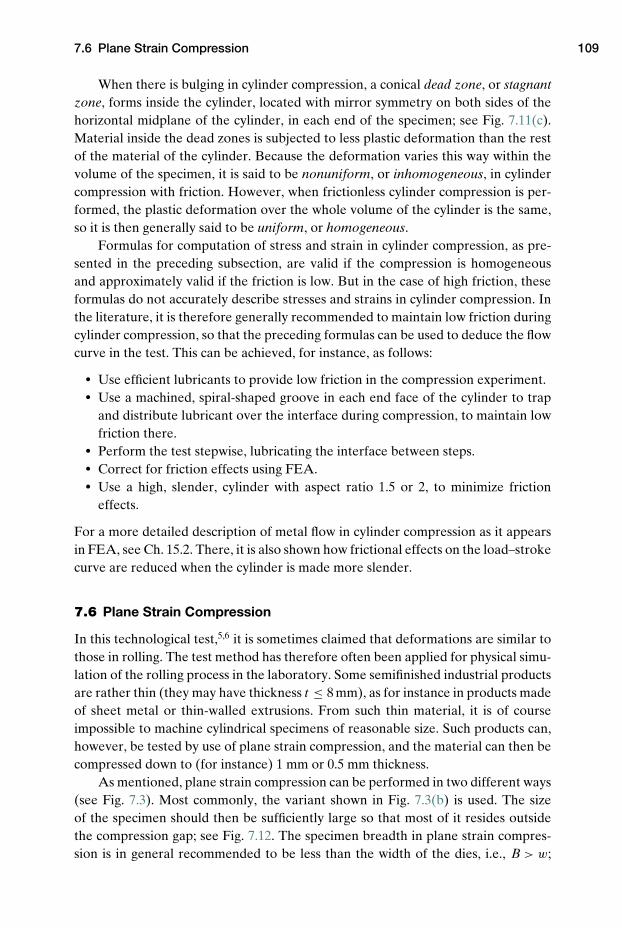
7.6 Plane Strain Compression 109
When there is bulging in cylinder compression, a conical dead zone, or stagnantzone, forms inside the cylinder, located with mirror symmetry on both sides of thehorizontal midplane of the cylinder, in each end of the specimen; see Fig. 7.11(c).Material inside the dead zones is subjected to less plastic deformation than the restof the material of the cylinder. Because the deformation varies this way within thevolume of the specimen, it is said to be nonuniform, or inhomogeneous, in cylindercompression with friction. However, when frictionless cylinder compression is per-formed, the plastic deformation over the whole volume of the cylinder is the same,so it is then generally said to be uniform, or homogeneous.
Formulas for computation of stress and strain in cylinder compression, as pre-sented in the preceding subsection, are valid if the compression is homogeneousand approximately valid if the friction is low. But in the case of high friction, theseformulas do not accurately describe stresses and strains in cylinder compression. Inthe literature, it is therefore generally recommended to maintain low friction duringcylinder compression, so that the preceding formulas can be used to deduce the flowcurve in the test. This can be achieved, for instance, as follows:
� Use efficient lubricants to provide low friction in the compression experiment.� Use a machined, spiral-shaped groove in each end face of the cylinder to trap
and distribute lubricant over the interface during compression, to maintain lowfriction there.
� Perform the test stepwise, lubricating the interface between steps.� Correct for friction effects using FEA.� Use a high, slender, cylinder with aspect ratio 1.5 or 2, to minimize friction
effects.
For a more detailed description of metal flow in cylinder compression as it appearsin FEA, see Ch. 15.2. There, it is also shown how frictional effects on the load–strokecurve are reduced when the cylinder is made more slender.
7.6 Plane Strain Compression
In this technological test,5,6 it is sometimes claimed that deformations are similar tothose in rolling. The test method has therefore often been applied for physical simu-lation of the rolling process in the laboratory. Some semifinished industrial productsare rather thin (they may have thickness t ≤ 8 mm), as for instance in products madeof sheet metal or thin-walled extrusions. From such thin material, it is of courseimpossible to machine cylindrical specimens of reasonable size. Such products can,however, be tested by use of plane strain compression, and the material can then becompressed down to (for instance) 1 mm or 0.5 mm thickness.
As mentioned, plane strain compression can be performed in two different ways(see Fig. 7.3). Most commonly, the variant shown in Fig. 7.3(b) is used. The sizeof the specimen should then be sufficiently large so that most of it resides outsidethe compression gap; see Fig. 7.12. The specimen breadth in plane strain compres-sion is in general recommended to be less than the width of the dies, i.e., B > w;
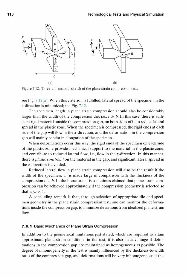
110 Technological Tests and Physical Simulation
(a) (b)
Figure 7.12. Three-dimensional sketch of the plane strain compression test.
see Fig. 7.12(a). When this criterion is fulfilled, lateral spread of the specimen in thez-direction is minimized; see Fig. 7.12.
The specimen length in plane strain compression should also be considerablylarger than the width of the compression die, i.e., l b. In this case, there is suffi-cient rigid material outside the compression gap, on both sides of it, to reduce lateralspread in the plastic zone. When the specimen is compressed, the rigid ends at eachside of the gap will flow in the x-direction, and the deformation in the compressiongap will mainly consist in elongation of the specimen.
When deformations occur this way, the rigid ends of the specimen on each sideof the plastic zone provide mechanical support to the material in the plastic zone,and contribute to reduced lateral flow, i.e., flow in the z-direction. In this manner,there is plastic constraint on the material in the gap, and significant lateral spread inthe z-direction is avoided.
Reduced lateral flow in plane strain compression will also be the result if thewidth of the specimen, w, is made large in comparison with the thickness of thecompression die, b. In the literature, it is sometimes claimed that plane strain com-pression can be achieved approximately if the compression geometry is selected sothat w/b > 5.
A concluding remark is that, through selection of appropriate die and speci-men geometry in the plane strain compression test, one can monitor the deforma-tions inside the compression gap, to minimize deviations from idealized plane strainflow.
7.6.1 Basic Mechanics of Plane Strain Compression
In addition to the geometrical limitations just stated, which are required to attainapproximate plane strain conditions in the test, it is also an advantage if defor-mations in the compression gap are maintained as homogeneous as possible. Thedegree of inhomogeneity in the test is mainly influenced by the thickness-to-widthratio of the compression gap, and deformations will be very inhomogeneous if this
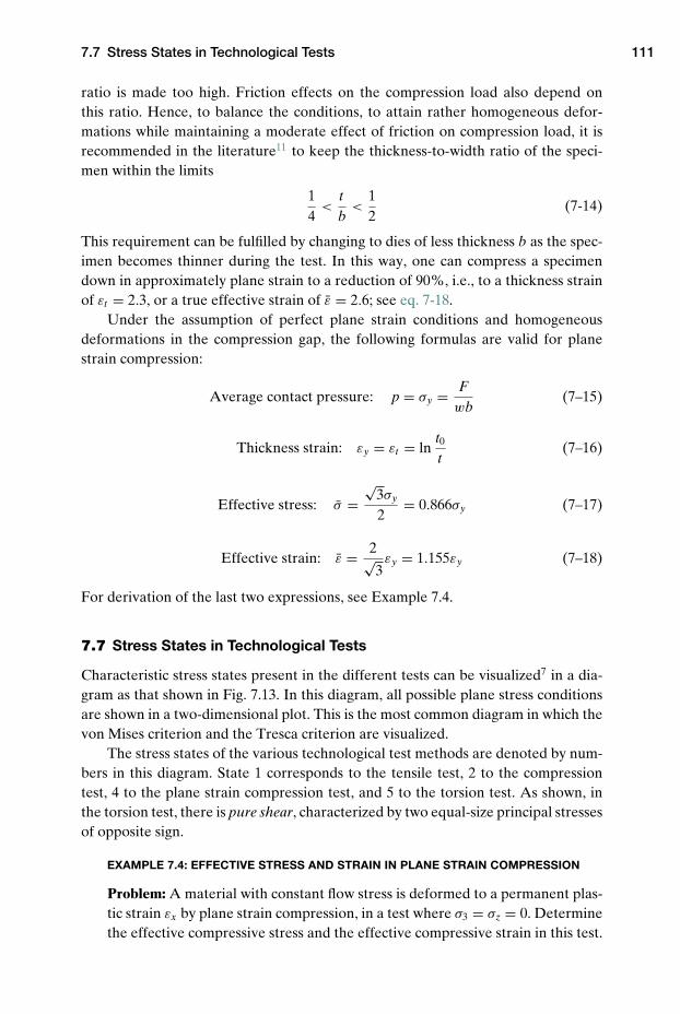
7.7 Stress States in Technological Tests 111
ratio is made too high. Friction effects on the compression load also depend onthis ratio. Hence, to balance the conditions, to attain rather homogeneous defor-mations while maintaining a moderate effect of friction on compression load, it isrecommended in the literature11 to keep the thickness-to-width ratio of the speci-men within the limits
14
<tb
<12
(7-14)
This requirement can be fulfilled by changing to dies of less thickness b as the spec-imen becomes thinner during the test. In this way, one can compress a specimendown in approximately plane strain to a reduction of 90%, i.e., to a thickness strainof εt = 2.3, or a true effective strain of ε = 2.6; see eq. 7-18.
Under the assumption of perfect plane strain conditions and homogeneousdeformations in the compression gap, the following formulas are valid for planestrain compression:
Average contact pressure: p = σy = Fwb
(7–15)
Thickness strain: εy = εt = lnt0t
(7–16)
Effective stress: σ =√
3σy
2= 0.866σy (7–17)
Effective strain: ε = 2√3εy = 1.155εy (7–18)
For derivation of the last two expressions, see Example 7.4.
7.7 Stress States in Technological Tests
Characteristic stress states present in the different tests can be visualized7 in a dia-gram as that shown in Fig. 7.13. In this diagram, all possible plane stress conditionsare shown in a two-dimensional plot. This is the most common diagram in which thevon Mises criterion and the Tresca criterion are visualized.
The stress states of the various technological test methods are denoted by num-bers in this diagram. State 1 corresponds to the tensile test, 2 to the compressiontest, 4 to the plane strain compression test, and 5 to the torsion test. As shown, inthe torsion test, there is pure shear, characterized by two equal-size principal stressesof opposite sign.
EXAMPLE 7.4: EFFECTIVE STRESS AND STRAIN IN PLANE STRAIN COMPRESSION
Problem: A material with constant flow stress is deformed to a permanent plas-tic strain εx by plane strain compression, in a test where σ3 = σz = 0. Determinethe effective compressive stress and the effective compressive strain in this test.
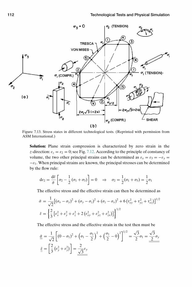
112 Technological Tests and Physical Simulation
Figure 7.13. Stress states in different technological tests. (Reprinted with permission fromASM International.)
Solution: Plane strain compression is characterized by zero strain in thez-direction: εz = ε2 = 0; see Fig. 7.12. According to the principle of constancy ofvolume, the two other principal strains can be determined as εx = ε3 = −εy =−ε1. When principal strains are known, the principal stresses can be determinedby the flow rule:
dε2 = dε
σ
[σ2 − 1
2(σ1 + σ3)
]= 0 ⇒ σ2 = 1
2(σ1 + σ3) = 1
2σ1
The effective stress and the effective strain can then be determined as
σ = 1√2
[(σx − σy)2 + (σy − σz)
2 + (σz − σx)2 + 6(τ 2
xy + τ 2yz + τ 2
xz
)]1/2
ε ={
23
[ε2
x + ε2y + ε2
z + 2(ε2
xy + ε2yz + ε2
zx
)]}1/2
The effective stress and the effective strain in the test then must be
σ = 1√2
[(0 − σ1)2 +
(σ1 − σ1
2
)2+
(σ1
2− 0
)2]1/2
=√
32
σ1 =√
32
σy
ε =[
23
(ε2
y + ε2y
)] = 2√3εy
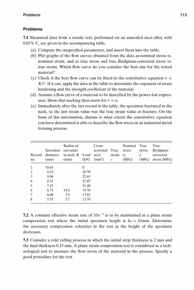
Problems 113
Problems
7.1 Measured data from a tensile test, performed on an annealed steel alloy with0.05% C, are given in the accompanying table.
(a) Compute the unspecified parameters, and insert them into the table.(b) Plot graphs of the flow curves obtained from the data as nominal stress vs.
nominal strain, and as true stress and true Bridgman-corrected stress vs.true strain. Which flow curve do you consider the best one for the testedmaterial?
(c) Check if the best flow curve can be fitted to the constitutive equation σ =Kεn. If it can, apply the data in the table to determine the exponent of strainhardening and the strength coefficient of the material.
(d) Assume a flow curve of a material to be described by the power-law expres-sion. Show that necking then starts for ε = n.
(e) Immediately after the last record in the table, the specimen fractured in theneck, so the last strain value was the true strain value at fracture. On thebasis of this information, discuss to what extent the constitutive equationyou have determined is able to describe the flow stress in an industrial metalforming process.
Radius of Cross- Nominal True TrueSpecimen curvature sectional True stress stress Bridgman-
Record diameter in neck, R Load area strain σn σ correctedno. (mm) (mm) (kN) (mm2) ε (MPa) (MPa) stress (MPa)
1 10.03 02 9.53 20.703 9.06 22.654 8.21 22.855 7.43 21.406 6.75 14.8 19.707 6.08 7.9 17.858 5.53 5.7 13.70
7.2 A constant effective strain rate of 10 s−1 is to be maintained in a plane straincompression test where the initial specimen height is h0 = 10 mm. Determinethe necessary compression velocities in the test as the height of the specimendecreases.
7.3 Consider a cold rolling process in which the initial strip thickness is 2 mm andthe final thickness 0.25 mm. A plane strain compression test is considered as a tech-nological test to measure the flow stress of the material in the process. Specify agood procedure for the test.
114 Technological Tests and Physical Simulation
NOTES
1. Ferguson, D., Chen, W., Bonesteel, T. and Vosburg, J.: “A look at physical simulationof metallurgical processes, past, present and future,” Materials Science and Engineering:A, Vol. 499, 2009, pp. 329–332.
2. Pohlandt, K.: “Materials Testing for the Metal Forming Industry,” Springer-Verlag,1989.
3. Dieter, G. E. (Ed.): “Workability Testing Techniques,” ASM Int., Metals Park, Ohio,1984.
4. Davis, J. R.: “Tensile testing,” ASM Int., Metals Park, Ohio, 2004.5. Silk, N. J., and Winden, M. R.: “Interpretation of hot plane strain compression testing of
aluminium specimens,” Materials Science and Technology, Vol. 15, 1999, pp. 295–300.6. Uyyuru, R. K.: “Plane strain compression test as a friction-measuring test – a compre-
hensive review,” Int. J. Forming Processes, Vol. 7, No. 3, 2004, pp. 310–319.7. Schey, J. A.: “Tribology in Metalworking; Friction, Lubrication and Wear,” ASM Int.,
Metals Park, Ohio, 1983, pp. 12–13.8. http://www.gleeble.com/9. Storojeva, L., Ponge, D., Kaspar, R., and Raabe, D.: “Development of microstructure
and texture of medium carbon steel during heavy warm deformation,” Acta Materialia,Vol. 52, 2004, pp. 2209–2220.
10. Bridgman, P. W.: “Stress distribution in the neck of a tension specimen,” Trans. Amer.Soc. Metals, Vol. 32, 1944, p. 553.
11. Dieter, G.: “Mechanical Metallurgy,” McGraw-Hill, 1989.
REFERENCE
“ASM Handbook, Vol. 8, Mechanical Testing and Evaluation,” ASM Int., Metals Park, Ohio,2000.
8 Flow Stress Data
The flow stress of a material is indeed an important parameter in metal forming. Tocreate a good FEM model of a forming process, for example, it is required that onebe able to specify the flow stress of the workpiece material with good accuracy.
Because of this, the main processing parameters affecting the flow stress of com-monly used metals and their alloys will be considered in this chapter, as regards bothcold and hot forming applications. When the flow stress has been measured, so oneknows how the processing parameters affect the flow stress, it is common to searchfor an equation that can describe the actual flow stress dependence well. When onehas arrived at such an equation, one says that one has obtained a good materialmodel for the material. It is also common to call the material model the constitutiveequation for the actual metal. Commonly applied procedures to determine constitu-tive equations for metals will be described and material models for some commonlyused metals will be reviewed in this chapter.
8.1 The Flow Stress
In Fig. 7.8(b), flow stress curves were shown as they commonly appear for a metalat room temperature. As depicted in this figure, the true flow stress often increaseswith increasing strain when the metal is tested at room temperature.
If we consider metals, at cold, warm, and hot forming temperatures, a numberof parameters can affect flow stress, not only strain. If possible, it is useful to expressthe flow stress by a function, instead of using only graphs, i.e., to express the flowstress in terms of a material model or a constitutive equation for the consideredmaterial.
8.2 Constitutive Equations for Metals
There are many different metals and alloys, but in this context, I will restrict thetreatment to common metals and to the more common constitutive equations.
Remember that at low strains the stress commonly has a linear relationship vs.strain, as described by Hooke’s law. The stress a material is subjected to can then be
115
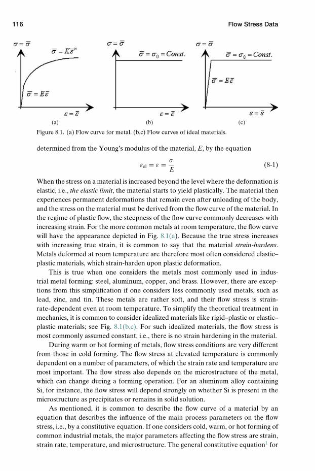
116 Flow Stress Data
(a) (b) (c)
Figure 8.1. (a) Flow curve for metal. (b,c) Flow curves of ideal materials.
determined from the Young’s modulus of the material, E, by the equation
εel = ε = σ
E(8-1)
When the stress on a material is increased beyond the level where the deformation iselastic, i.e., the elastic limit, the material starts to yield plastically. The material thenexperiences permanent deformations that remain even after unloading of the body,and the stress on the material must be derived from the flow curve of the material. Inthe regime of plastic flow, the steepness of the flow curve commonly decreases withincreasing strain. For the more common metals at room temperature, the flow curvewill have the appearance depicted in Fig. 8.1(a). Because the true stress increaseswith increasing true strain, it is common to say that the material strain-hardens.Metals deformed at room temperature are therefore most often considered elastic–plastic materials, which strain-harden upon plastic deformation.
This is true when one considers the metals most commonly used in indus-trial metal forming: steel, aluminum, copper, and brass. However, there are excep-tions from this simplification if one considers less commonly used metals, such aslead, zinc, and tin. These metals are rather soft, and their flow stress is strain-rate-dependent even at room temperature. To simplify the theoretical treatment inmechanics, it is common to consider idealized materials like rigid–plastic or elastic–plastic materials; see Fig. 8.1(b,c). For such idealized materials, the flow stress ismost commonly assumed constant, i.e., there is no strain hardening in the material.
During warm or hot forming of metals, flow stress conditions are very differentfrom those in cold forming. The flow stress at elevated temperature is commonlydependent on a number of parameters, of which the strain rate and temperature aremost important. The flow stress also depends on the microstructure of the metal,which can change during a forming operation. For an aluminum alloy containingSi, for instance, the flow stress will depend strongly on whether Si is present in themicrostructure as precipitates or remains in solid solution.
As mentioned, it is common to describe the flow curve of a material by anequation that describes the influence of the main process parameters on the flowstress, i.e., by a constitutive equation. If one considers cold, warm, or hot forming ofcommon industrial metals, the major parameters affecting the flow stress are strain,strain rate, temperature, and microstructure. The general constitutive equation1 for
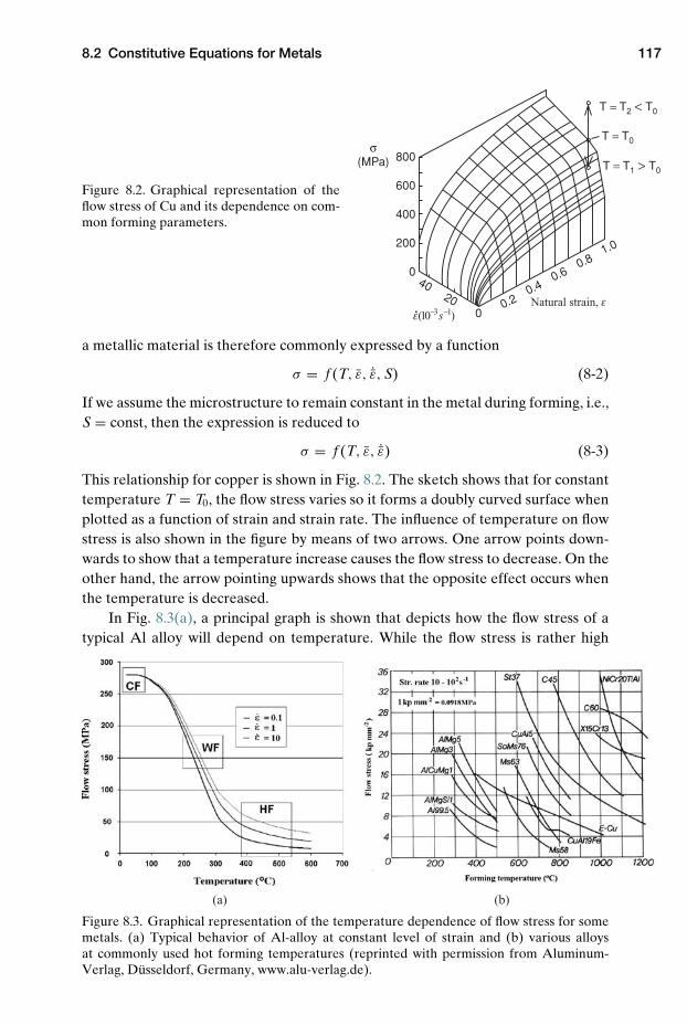
8.2 Constitutive Equations for Metals 117
800
600
400
200
0
T = T2 < T0
T = T1 > T0
T = T0
4020
00.2
0.40.6
0.81.0
Natural strain, εε•(10−3 s−1)
σ (MPa)
Figure 8.2. Graphical representation of theflow stress of Cu and its dependence on com-mon forming parameters.
a metallic material is therefore commonly expressed by a function
σ = f (T, ε, ˙ε, S) (8-2)
If we assume the microstructure to remain constant in the metal during forming, i.e.,S = const, then the expression is reduced to
σ = f (T, ε, ˙ε) (8-3)
This relationship for copper is shown in Fig. 8.2. The sketch shows that for constanttemperature T = T0, the flow stress varies so it forms a doubly curved surface whenplotted as a function of strain and strain rate. The influence of temperature on flowstress is also shown in the figure by means of two arrows. One arrow points down-wards to show that a temperature increase causes the flow stress to decrease. On theother hand, the arrow pointing upwards shows that the opposite effect occurs whenthe temperature is decreased.
In Fig. 8.3(a), a principal graph is shown that depicts how the flow stress of atypical Al alloy will depend on temperature. While the flow stress is rather high
(a) (b)
Figure 8.3. Graphical representation of the temperature dependence of flow stress for somemetals. (a) Typical behavior of Al-alloy at constant level of strain and (b) various alloysat commonly used hot forming temperatures (reprinted with permission from Aluminum-Verlag, Dusseldorf, Germany, www.alu-verlag.de).
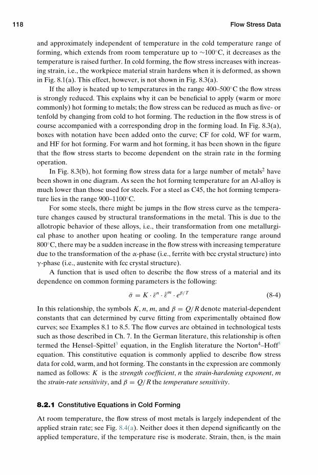
118 Flow Stress Data
and approximately independent of temperature in the cold temperature range offorming, which extends from room temperature up to ∼100◦C, it decreases as thetemperature is raised further. In cold forming, the flow stress increases with increas-ing strain, i.e., the workpiece material strain hardens when it is deformed, as shownin Fig. 8.1(a). This effect, however, is not shown in Fig. 8.3(a).
If the alloy is heated up to temperatures in the range 400–500◦C the flow stressis strongly reduced. This explains why it can be beneficial to apply (warm or morecommonly) hot forming to metals; the flow stress can be reduced as much as five- ortenfold by changing from cold to hot forming. The reduction in the flow stress is ofcourse accompanied with a corresponding drop in the forming load. In Fig. 8.3(a),boxes with notation have been added onto the curve; CF for cold, WF for warm,and HF for hot forming. For warm and hot forming, it has been shown in the figurethat the flow stress starts to become dependent on the strain rate in the formingoperation.
In Fig. 8.3(b), hot forming flow stress data for a large number of metals2 havebeen shown in one diagram. As seen the hot forming temperature for an Al-alloy ismuch lower than those used for steels. For a steel as C45, the hot forming tempera-ture lies in the range 900–1100◦C.
For some steels, there might be jumps in the flow stress curve as the tempera-ture changes caused by structural transformations in the metal. This is due to theallotropic behavior of these alloys, i.e., their transformation from one metallurgi-cal phase to another upon heating or cooling. In the temperature range around800◦C, there may be a sudden increase in the flow stress with increasing temperaturedue to the transformation of the α-phase (i.e., ferrite with bcc crystal structure) intoγ-phase (i.e., austenite with fcc crystal structure).
A function that is used often to describe the flow stress of a material and itsdependence on common forming parameters is the following:
σ = K · εn · ˙εm · eβ/T (8-4)
In this relationship, the symbols K, n, m, and β = Q/R denote material-dependentconstants that can determined by curve fitting from experimentally obtained flowcurves; see Examples 8.1 to 8.5. The flow curves are obtained in technological testssuch as those described in Ch. 7. In the German literature, this relationship is oftentermed the Hensel–Spittel3 equation, in the English literature the Norton4–Hoff5
equation. This constitutive equation is commonly applied to describe flow stressdata for cold, warm, and hot forming. The constants in the expression are commonlynamed as follows: K is the strength coefficient, n the strain-hardening exponent, mthe strain-rate sensitivity, and β = Q/R the temperature sensitivity.
8.2.1 Constitutive Equations in Cold Forming
At room temperature, the flow stress of most metals is largely independent of theapplied strain rate; see Fig. 8.4(a). Neither does it then depend significantly on theapplied temperature, if the temperature rise is moderate. Strain, then, is the main
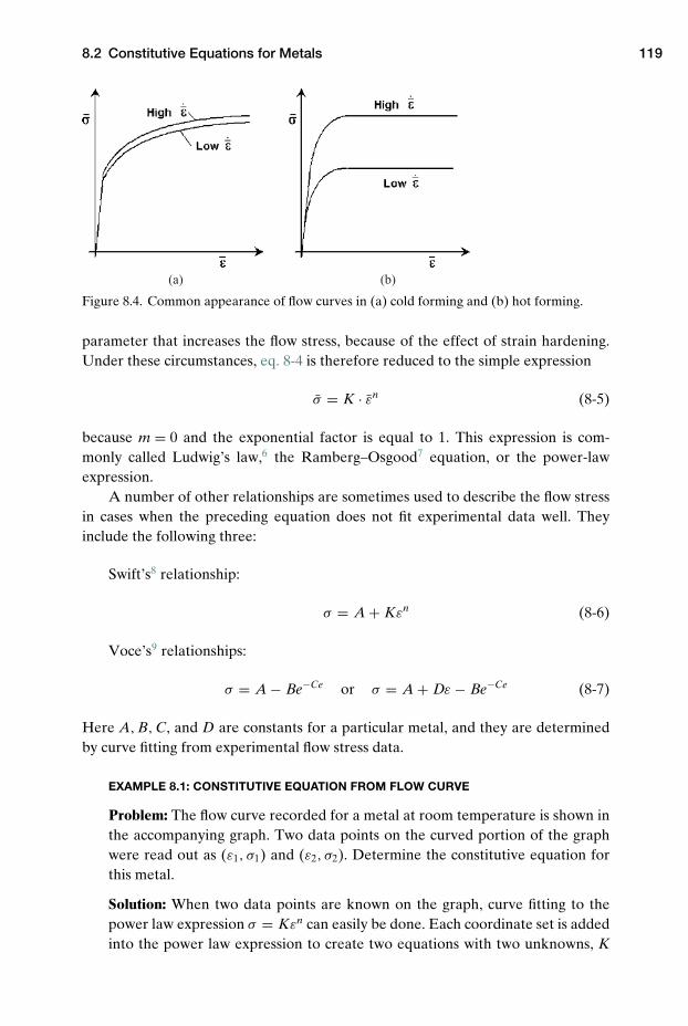
8.2 Constitutive Equations for Metals 119
(a) (b)
Figure 8.4. Common appearance of flow curves in (a) cold forming and (b) hot forming.
parameter that increases the flow stress, because of the effect of strain hardening.Under these circumstances, eq. 8-4 is therefore reduced to the simple expression
σ = K · εn (8-5)
because m = 0 and the exponential factor is equal to 1. This expression is com-monly called Ludwig’s law,6 the Ramberg–Osgood7 equation, or the power-lawexpression.
A number of other relationships are sometimes used to describe the flow stressin cases when the preceding equation does not fit experimental data well. Theyinclude the following three:
Swift’s8 relationship:
σ = A + Kεn (8-6)
Voce’s9 relationships:
σ = A − Be−Ce or σ = A + Dε − Be−Ce (8-7)
Here A, B, C, and D are constants for a particular metal, and they are determinedby curve fitting from experimental flow stress data.
EXAMPLE 8.1: CONSTITUTIVE EQUATION FROM FLOW CURVE
Problem: The flow curve recorded for a metal at room temperature is shown inthe accompanying graph. Two data points on the curved portion of the graphwere read out as (ε1, σ1) and (ε2, σ2). Determine the constitutive equation forthis metal.
Solution: When two data points are known on the graph, curve fitting to thepower law expression σ = Kεn can easily be done. Each coordinate set is addedinto the power law expression to create two equations with two unknowns, K
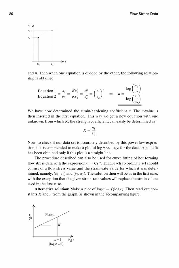
120 Flow Stress Data
σ2
σ
σ1
ε1 ε2ε
and n. Then when one equation is divided by the other, the following relation-ship is obtained:
Equation 1Equation 2
= σ1
σ2= Kεn
1
Kεn2
= εn1
εn2
=(
ε1
ε2
)n
⇒ n =log
(σ1
σ2
)
log(
ε1
ε2
)
We have now determined the strain-hardening coefficient n. The n-value isthen inserted in the first equation. This way we get a new equation with oneunknown, from which K, the strength coefficient, can easily be determined as
K = σ1
εn1
Now, to check if our data set is accurately described by this power law expres-sion, it is recommended to make a plot of log σ vs. log ε for the data. A good fithas been obtained only if this plot is a straight line.
The procedure described can also be used for curve fitting of hot formingflow stress data with the expression σ = Cεm. Then, each co ordinate set shouldconsist of a flow stress value and the strain-rate value for which it was deter-mined, namely, (ε1, σ1) and (ε2, σ2). The solution then will be as in the first case,with the exception that the given strain-rate values will replace the strain valuesused in the first case.
Alternative solution: Make a plot of log σ = f (log ε). Then read out con-stants K and n from the graph, as shown in the accompanying figure.
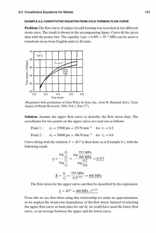
8.2 Constitutive Equations for Metals 121
EXAMPLE 8.2: CONSTITUTIVE EQUATION FROM COLD FORMING FLOW CURVE
Problem: The flow curve of copper in cold forming was recorded at two differentstrain rates. The result is shown in the accompanying figure. Curve-fit the givendata with the power law. The equality 1 psi = 6.895 × 10⁻³ MPa can be used totransform stress from English units to SI units.
70
60
50
40
30
200.0 0.2 0.4
18°C
Low strain rate
0.6 0.8True strain
True
str
ess
(100
0psi
)
ε•= 23 s-1
(Reprinted with permission of John Wiley & Sons, Inc., from R. Bunshah (Ed.), Tech-niques of Metals Research, 1968, Vol. 1, Part 310).
Solution: Assume the upper flow curve to describe the flow stress data. Thecoordinates for two points on the upper curve are read out as follows:
Point 1 : σ1 = 37000 psi = 255 N mm−2 for ε1 = 0.2
Point 2 : σ2 = 56000 psi = 386 N mm−2 for ε2 = 0.6
Curve fitting with the relation: σ = Kεn is then done as in Example 8.1, with thefollowing result:
n =log
σ1
σ2
logε1
ε2
=log
255 MPa386 MPa
log0.20.6
= 0.377
K = σ1
εn1
= 255 MPa0.20.377
= 468 MPa
The flow stress for the upper curve can then be described by the expression
σ = Kεn = 468 MPa · ε0,377
From this we see that when using this relationship we make an approximation,as we neglect the strain-rate dependence of the flow stress. Instead of selectingthe upper flow curve as basis data for our fit, we could have used the lower flowcurve, or an average between the upper and the lower curve.
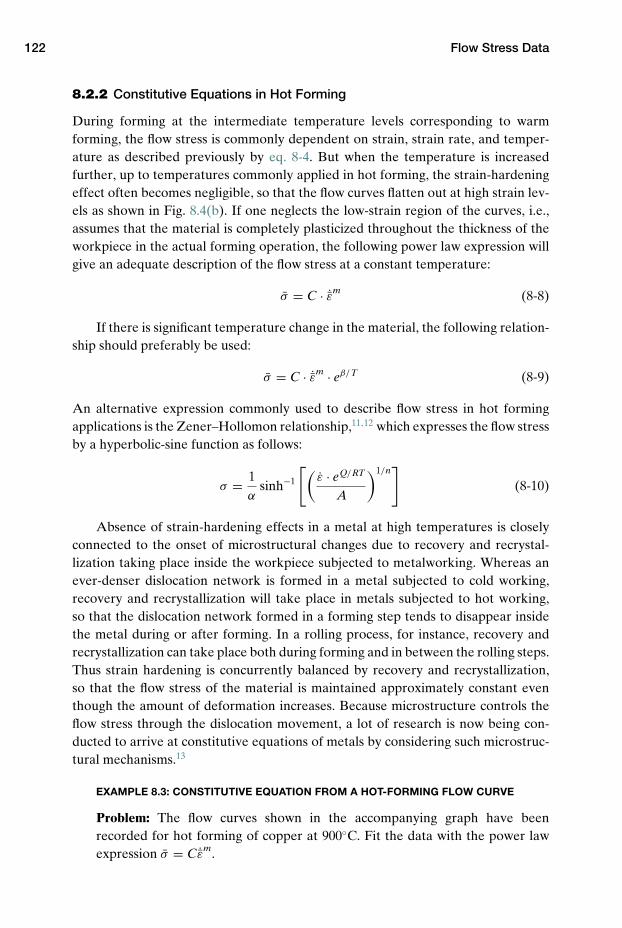
122 Flow Stress Data
8.2.2 Constitutive Equations in Hot Forming
During forming at the intermediate temperature levels corresponding to warmforming, the flow stress is commonly dependent on strain, strain rate, and temper-ature as described previously by eq. 8-4. But when the temperature is increasedfurther, up to temperatures commonly applied in hot forming, the strain-hardeningeffect often becomes negligible, so that the flow curves flatten out at high strain lev-els as shown in Fig. 8.4(b). If one neglects the low-strain region of the curves, i.e.,assumes that the material is completely plasticized throughout the thickness of theworkpiece in the actual forming operation, the following power law expression willgive an adequate description of the flow stress at a constant temperature:
σ = C · ˙εm (8-8)
If there is significant temperature change in the material, the following relation-ship should preferably be used:
σ = C · ˙εm · eβ/T (8-9)
An alternative expression commonly used to describe flow stress in hot formingapplications is the Zener–Hollomon relationship,11,12 which expresses the flow stressby a hyperbolic-sine function as follows:
σ = 1α
sinh−1
[(ε · eQ/RT
A
)1/n]
(8-10)
Absence of strain-hardening effects in a metal at high temperatures is closelyconnected to the onset of microstructural changes due to recovery and recrystal-lization taking place inside the workpiece subjected to metalworking. Whereas anever-denser dislocation network is formed in a metal subjected to cold working,recovery and recrystallization will take place in metals subjected to hot working,so that the dislocation network formed in a forming step tends to disappear insidethe metal during or after forming. In a rolling process, for instance, recovery andrecrystallization can take place both during forming and in between the rolling steps.Thus strain hardening is concurrently balanced by recovery and recrystallization,so that the flow stress of the material is maintained approximately constant eventhough the amount of deformation increases. Because microstructure controls theflow stress through the dislocation movement, a lot of research is now being con-ducted to arrive at constitutive equations of metals by considering such microstruc-tural mechanisms.13
EXAMPLE 8.3: CONSTITUTIVE EQUATION FROM A HOT-FORMING FLOW CURVE
Problem: The flow curves shown in the accompanying graph have beenrecorded for hot forming of copper at 900◦C. Fit the data with the power lawexpression σ = C ˙εm.
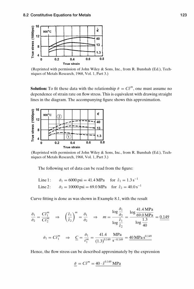
8.2 Constitutive Equations for Metals 123
(Reprinted with permission of John Wiley & Sons, Inc., from R. Bunshah (Ed.), Tech-niques of Metals Research, 1968, Vol. 1, Part 3.)
Solution: To fit these data with the relationship σ = C ˙εm, one must assume nodependence of strain rate on flow stress. This is equivalent with drawing straightlines in the diagram. The accompanying figure shows this approximation.
(Reprinted with permission of John Wiley & Sons, Inc., from R. Bunshah (Ed.), Tech-niques of Metals Research, 1968, Vol. 1, Part 3.)
The following set of data can be read from the figure:
Line 1: σ1 = 6000 psi = 41.4 MPa for ˙ε1 = 1.3 s−1
Line 2: σ2 = 10000 psi = 69.0 MPa for ˙ε2 = 40.0 s−1
Curve fitting is done as was shown in Example 8.1, with the result
σ1
σ2= C ˙εm
1
C ˙εm2
⇒( ˙ε1
˙ε2
)m
= σ1
σ2⇒ m =
logσ1
σ2
log˙ε1
˙ε2
=log
41.4 MPa69.0 MPa
log1.340
= 0.149
σ1 = C ˙εm1 ⇒ C = σ1
εm1
= 41.4
(1.3)0.149
MPas−0.149
= 40 MPa s0.149
Hence, the flow stress can be described approximately by the expression
σ = C ˙εm = 40 · ˙ε0.149 MPa

124 Flow Stress Data
EXAMPLE 8.4: NORTON–HOFF CONSTITUTIVE EQUATION FROM HOT-FORMING FLOW
STRESS DATA
Problem: Fit the flow stress data given in the accompanying table with theNorton–Hoff constitutive equation.
T ε σ
(◦C) ε (s−1) (MPa)
350 0.5 1 71425 0.5 1 43500 0.5 1 29350 0.5 10 99425 0.5 10 60500 0.5 10 40350 1 1 81425 1 1 49500 1 1 31350 1 10 109425 1 10 66500 1 10 42
Solution: This problem can be solved by using an Excel spreadsheet. The dataare first inserted into different columns of the spreadsheet.
If we take the natural logarithm of the constitutive equation to be used, weget the following linear expression:
ln σ = ln K + n ln ε + m ln ε + β1T
A linear regression analysis can then be done by means of the spreadsheet,based on the data in the table. An Excel spreadsheet that shows this regressionanalysis is available at www.cambridge.org/valberg.
The result of the regression analysis is
ln σ = −0.40247 + 0.136914ε + 0.136483ε + 2979.473T
≈ −0.402 + 0.137ε + 0.136ε + 2979.5T
Thus the following constitutive equation is obtained for the given data set:
σ = 0.669 · ε0.137 · ε0.136 · e2979.5/T
EXAMPLE 8.5: ZENER–HOLLOMON CONSTITUTIVE EQUATION FROM HOT-FORMING
FLOW STRESS DATA
Problem: Fit the flow stress data in the accompanying table with the Zener–Hollomon constitutive equation.
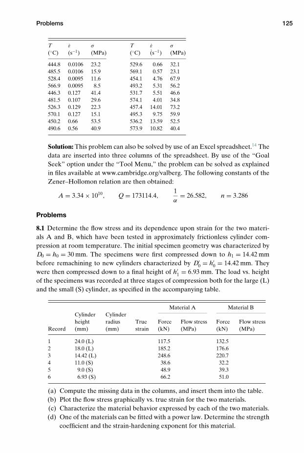
Problems 125
T ε σ T ε σ
(◦C) (s−1) (MPa) (◦C) (s−1) (MPa)
444.8 0.0106 23.2 529.6 0.66 32.1485.5 0.0106 15.9 569.1 0.57 23.1528.4 0.0095 11.6 454.1 4.76 67.9566.9 0.0095 8.5 493.2 5.31 56.2446.3 0.127 41.4 531.7 5.51 46.6481.5 0.107 29.6 574.1 4.01 34.8526.3 0.129 22.3 457.4 14.01 73.2570.1 0.127 15.1 495.3 9.75 59.9450.2 0.66 53.5 536.2 13.59 52.5490.6 0.56 40.9 573.9 10.82 40.4
Solution: This problem can also be solved by use of an Excel spreadsheet.14 Thedata are inserted into three columns of the spreadsheet. By use of the “GoalSeek” option under the “Tool Menu,” the problem can be solved as explainedin files available at www.cambridge.org/valberg. The following constants of theZener–Hollomon relation are then obtained:
A = 3.34 × 10¹⁰, Q = 173114.4,1α
= 26.582, n = 3.286
Problems
8.1 Determine the flow stress and its dependence upon strain for the two materi-als A and B, which have been tested in approximately frictionless cylinder com-pression at room temperature. The initial specimen geometry was characterized byD0 = h0 = 30 mm. The specimens were first compressed down to h1 = 14.42 mmbefore remachining to new cylinders characterized by D′
0 = h′0 = 14.42 mm. They
were then compressed down to a final height of h′1 = 6.93 mm. The load vs. height
of the specimens was recorded at three stages of compression both for the large (L)and the small (S) cylinder, as specified in the accompanying table.
Material A Material BCylinder Cylinderheight radius True Force Flow stress Force Flow stress
Record (mm) (mm) strain (kN) (MPa) (kN) (MPa)
1 24.0 (L) 117.5 132.52 18.0 (L) 185.2 176.63 14.42 (L) 248.6 220.74 11.0 (S) 38.6 32.25 9.0 (S) 48.9 39.36 6.93 (S) 66.2 51.0
(a) Compute the missing data in the columns, and insert them into the table.(b) Plot the flow stress graphically vs. true strain for the two materials.(c) Characterize the material behavior expressed by each of the two materials.(d) One of the materials can be fitted with a power law. Determine the strength
coefficient and the strain-hardening exponent for this material.
126 Flow Stress Data
(e) Specify the strain range for which the material model is valid.(f) Comment upon use of the obtained flow stress data for various metal form-
ing applications.
8.2 A cylinder is compressed between two plane parallel dies. The velocity of theupper die was kept constant at 10 mm s−1 while the lower die remained stationary.The initial specimen height was 30 mm, and the final height was 15 mm.
(a) Determine the effective strain and the effective strain rate applied in thistest for cylinder heights of 30, 25, 20, and 15 mm.
(b) Plot a graph of the strain and the strain rate in the test as functions of thestroke.
(c) Add an abscissa axis the graph to depict the height of the specimen.(d) Propose different means for obtaining constant strain rate in the compres-
sion test.
NOTES
1. Altan, T., Oh, S.-I., and Gegel, H. L.: “Metal Forming, Fundamentals and Applications,”ASM Int., 1983, pp. 45–73.
2. Laue, K., and Stenger, H.: “Strangpressen; Verfahren – Maschinen – Werkzeuge,”Aluminum-Verlag, Dusseldorf, 1976, p. 39.
3. Hensel, A., and Spittel, T.: “Arbeitsbedarf der bilsamen Formgebungsverfahren zumAufname von Fliesskurven,” VEB Deutscher Verlag fur Grundstoffindustrie, Leipzig,1978 (in German).
4. Norton, F. H.: “The Creep of Steel at High Temperature,” McGraw-Hill, New York,1929.
5. Hoff, H. J.: “Approximate analysis of structures in presence of moderately large creepdeformations,” Quart. Appl. Mathematics, Vol. 12, 1954, p. 49.
6. Ludwik, P.: “Elemente der Technologishen Mechanik,” Springer Verlag, Berlin, 1909(in German).
7. Ramberg, W., and Osgood, W. R., “Description of Stress–Strain Curves by Three Param-eters,” Technical Note no. 902, National Advisory Committee for Aeronautics, Washing-ton, DC, 1943.
8. Swift, H. W.: J. Mechanics and Physics of Solids, Vol. 1, 1952, pp. 1–18.9. Voce, E.: J. Institute of Metals, Vol. 74, 1948, pp. 537–562.
10. Schey, J. A.; “The more common fabrication processes,” Ch. 34 in R. F. Bunshah (Ed.):“Techniques of Metals Research,” Part 3; Techniques of materials preparation and han-dling, Interscience Publishers, 1968, p. 1429.
11. Zener, C., and Holloman, J. H., J. Appl. Physics, Vol. 15, 1944, pp. 22–32.12. Sellars, C. M., and Tegart, W. J. M. Mem. Sci. Rev. Metallurgie, Vol. 63, 1966, p. 731.13. Domkin, C.: “Constitutive Models Based on Dislocation Density,” Doctoral thesis,
Lulea Univ. of Technology, 2005.14. Roenning, B.: “Constitutive equations for AlZnMg-, AlZnMgCr- and AlZnMgZr-
alloys,” Ph.D. thesis, Norwegian Univ. of Science and Technology, 1998.
REFERENCES
Altan, T., Oh, S.-I., and Gegel, H. L.: “Metal forming, fundamentals and applications,” ASMInt., 1983, pp. 45–73.
Boyer, E. H. (Ed.): “Atlas of stress-strain curves,” 2nd ed., ASM Int., Metals Park, Ohio,2002.

9 Formability and Workability
In connection with the discussion of technological tests in Ch. 7, it was stated thatthe tensile test specimen after some degree of stretching tends to become unstable,due to the onset of necking. With further stretching, there is neck growth in thespecimen, and finally a fracture is formed in the neck, so that the specimen breaksinto two pieces.
When compression testing was discussed, it was stated that for ductile metals,larger strains can in general be obtained in this test than in tensile testing, becauseneck formation is avoided in compression. But also in the compression test thereare limitations on how much the specimen can be deformed. This is because variouscracking phenomena may occur, especially when low-ductility materials are tested.
In metal forming, it is a common problem that the material of the workpiecebreaks down during forming, in a manner like that for materials subjected to tech-nological tests. In this chapter, different phenomena that cause material failure dur-ing metal forming operations will be discussed, with special emphasis on failure dueto necking, tensile stress cracking, and shear cracking.
9.1 Formability and Workability
Formability and workability are terms that refer to the property of a material withregard to its ability to be shaped in metal forming without breakdown1 during theforming operation. Formability is most commonly used to describe how much amaterial can be formed in sheet-metal forming processes without losing its integrity,i.e., without being subjected to excessive thinning or fracture during forming. Work-ability, on the other hand, refers to the ability of a material to be formed in bulk-metal forming processes without breakdown of the material due to formation ofcracks of any kind. Such breakdown could be caused by partial or full fracture ofthe material. Partial fracture can occur close to the surface or in the interior of thebody subjected to forming, so that surface or internal cracks are formed. It is natu-ral to distinguish between crack formation in sheet-metal and in bulk-metal form-ing, because it is quite different phenomena that cause metal breakdown in eachcategory of process.
127
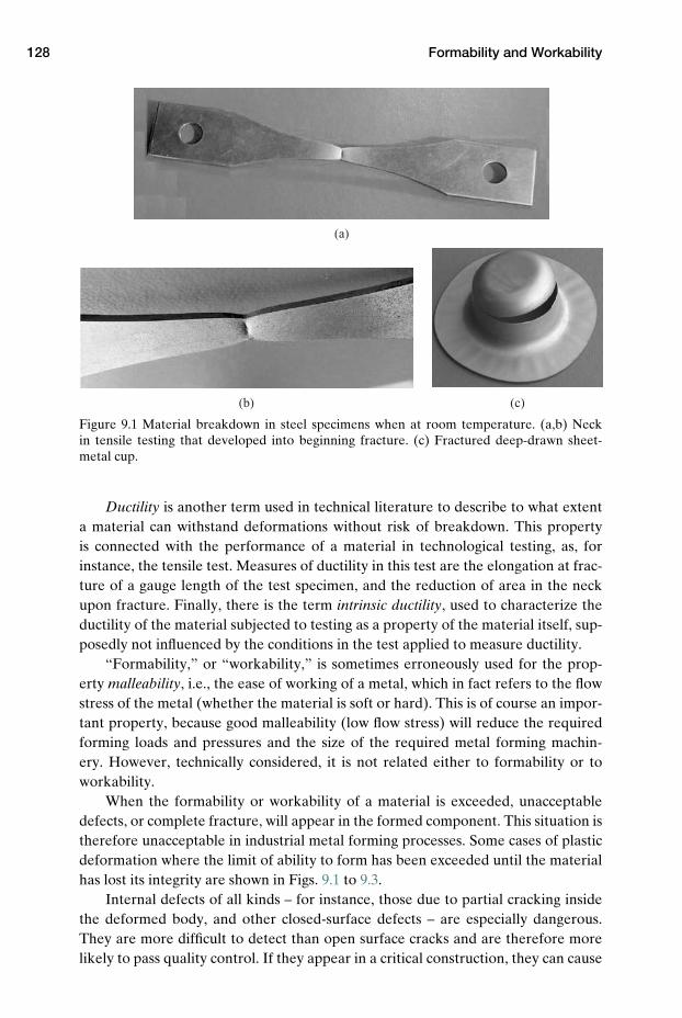
128 Formability and Workability
(a)
(b) (c)
Figure 9.1 Material breakdown in steel specimens when at room temperature. (a,b) Neckin tensile testing that developed into beginning fracture. (c) Fractured deep-drawn sheet-metal cup.
Ductility is another term used in technical literature to describe to what extenta material can withstand deformations without risk of breakdown. This propertyis connected with the performance of a material in technological testing, as, forinstance, the tensile test. Measures of ductility in this test are the elongation at frac-ture of a gauge length of the test specimen, and the reduction of area in the neckupon fracture. Finally, there is the term intrinsic ductility, used to characterize theductility of the material subjected to testing as a property of the material itself, sup-posedly not influenced by the conditions in the test applied to measure ductility.
“Formability,” or “workability,” is sometimes erroneously used for the prop-erty malleability, i.e., the ease of working of a metal, which in fact refers to the flowstress of the metal (whether the material is soft or hard). This is of course an impor-tant property, because good malleability (low flow stress) will reduce the requiredforming loads and pressures and the size of the required metal forming machin-ery. However, technically considered, it is not related either to formability or toworkability.
When the formability or workability of a material is exceeded, unacceptabledefects, or complete fracture, will appear in the formed component. This situation istherefore unacceptable in industrial metal forming processes. Some cases of plasticdeformation where the limit of ability to form has been exceeded until the materialhas lost its integrity are shown in Figs. 9.1 to 9.3.
Internal defects of all kinds – for instance, those due to partial cracking insidethe deformed body, and other closed-surface defects – are especially dangerous.They are more difficult to detect than open surface cracks and are therefore morelikely to pass quality control. If they appear in a critical construction, they can cause
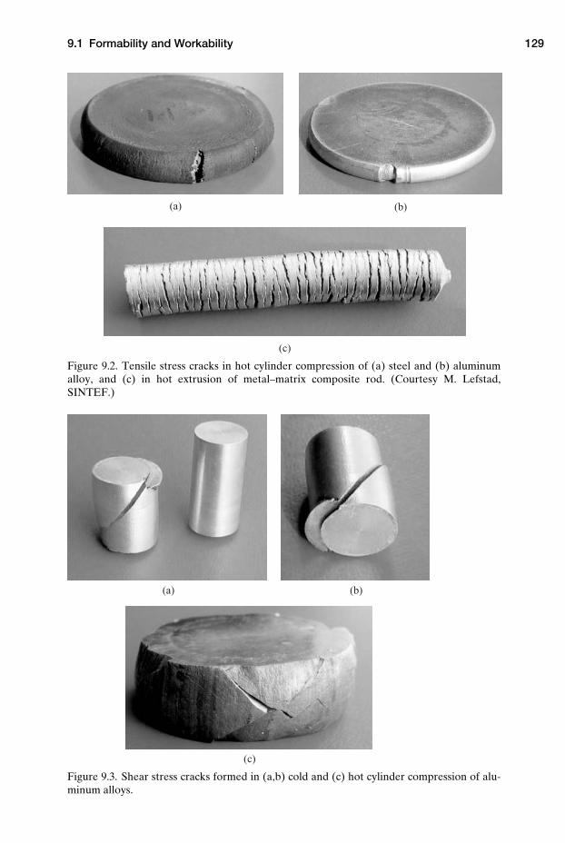
9.1 Formability and Workability 129
(a) (b)
(c)
Figure 9.2. Tensile stress cracks in hot cylinder compression of (a) steel and (b) aluminumalloy, and (c) in hot extrusion of metal–matrix composite rod. (Courtesy M. Lefstad,SINTEF.)
(a) (b)
(c)
Figure 9.3. Shear stress cracks formed in (a,b) cold and (c) hot cylinder compression of alu-minum alloys.
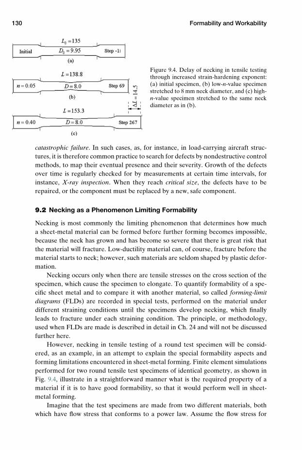
130 Formability and Workability
Figure 9.4. Delay of necking in tensile testingthrough increased strain-hardening exponent:(a) initial specimen, (b) low-n-value specimenstretched to 8 mm neck diameter, and (c) high-n-value specimen stretched to the same neckdiameter as in (b).
catastrophic failure. In such cases, as, for instance, in load-carrying aircraft struc-tures, it is therefore common practice to search for defects by nondestructive controlmethods, to map their eventual presence and their severity. Growth of the defectsover time is regularly checked for by measurements at certain time intervals, forinstance, X-ray inspection. When they reach critical size, the defects have to berepaired, or the component must be replaced by a new, safe component.
9.2 Necking as a Phenomenon Limiting Formability
Necking is most commonly the limiting phenomenon that determines how mucha sheet-metal material can be formed before further forming becomes impossible,because the neck has grown and has become so severe that there is great risk thatthe material will fracture. Low-ductility material can, of course, fracture before thematerial starts to neck; however, such materials are seldom shaped by plastic defor-mation.
Necking occurs only when there are tensile stresses on the cross section of thespecimen, which cause the specimen to elongate. To quantify formability of a spe-cific sheet metal and to compare it with another material, so called forming-limitdiagrams (FLDs) are recorded in special tests, performed on the material underdifferent straining conditions until the specimens develop necking, which finallyleads to fracture under each straining condition. The principle, or methodology,used when FLDs are made is described in detail in Ch. 24 and will not be discussedfurther here.
However, necking in tensile testing of a round test specimen will be consid-ered, as an example, in an attempt to explain the special formability aspects andforming limitations encountered in sheet-metal forming. Finite element simulationsperformed for two round tensile test specimens of identical geometry, as shown inFig. 9.4, illustrate in a straightforward manner what is the required property of amaterial if it is to have good formability, so that it would perform well in sheet-metal forming.
Imagine that the test specimens are made from two different materials, bothwhich have flow stress that conforms to a power law. Assume the flow stress for
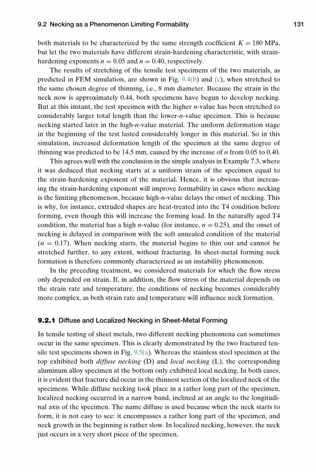
9.2 Necking as a Phenomenon Limiting Formability 131
both materials to be characterized by the same strength coefficient K = 180 MPa,but let the two materials have different strain-hardening characteristic, with strain-hardening exponents n = 0.05 and n = 0.40, respectively.
The results of stretching of the tensile test specimens of the two materials, aspredicted in FEM simulation, are shown in Fig. 9.4(b) and (c), when stretched tothe same chosen degree of thinning, i.e., 8 mm diameter. Because the strain in theneck now is approximately 0.44, both specimens have begun to develop necking.But at this instant, the test specimen with the higher n-value has been stretched toconsiderably larger total length than the lower-n-value specimen. This is becausenecking started later in the high-n-value material. The uniform deformation stagein the beginning of the test lasted considerably longer in this material. So in thissimulation, increased deformation length of the specimen at the same degree ofthinning was predicted to be 14.5 mm, caused by the increase of n from 0.05 to 0.40.
This agrees well with the conclusion in the simple analysis in Example 7.3, whereit was deduced that necking starts at a uniform strain of the specimen equal tothe strain-hardening exponent of the material. Hence, it is obvious that increas-ing the strain-hardening exponent will improve formability in cases where neckingis the limiting phenomenon, because high-n-value delays the onset of necking. Thisis why, for instance, extruded shapes are heat-treated into the T4 condition beforeforming, even though this will increase the forming load. In the naturally aged T4condition, the material has a high n-value (for instance, n = 0.25), and the onset ofnecking is delayed in comparison with the soft annealed condition of the material(n = 0.17). When necking starts, the material begins to thin out and cannot bestretched further, to any extent, without fracturing. In sheet-metal forming neckformation is therefore commonly characterized as an instability phenomenon.
In the preceding treatment, we considered materials for which the flow stressonly depended on strain. If, in addition, the flow stress of the material depends onthe strain rate and temperature, the conditions of necking becomes considerablymore complex, as both strain rate and temperature will influence neck formation.
9.2.1 Diffuse and Localized Necking in Sheet-Metal Forming
In tensile testing of sheet metals, two different necking phenomena can sometimesoccur in the same specimen. This is clearly demonstrated by the two fractured ten-sile test specimens shown in Fig. 9.5(a). Whereas the stainless steel specimen at thetop exhibited both diffuse necking (D) and local necking (L), the correspondingaluminum alloy specimen at the bottom only exhibited local necking. In both cases,it is evident that fracture did occur in the thinnest section of the localized neck of thespecimens. While diffuse necking took place in a rather long part of the specimen,localized necking occurred in a narrow band, inclined at an angle to the longitudi-nal axis of the specimen. The name diffuse is used because when the neck starts toform, it is not easy to see: it encompasses a rather long part of the specimen, andneck growth in the beginning is rather slow. In localized necking, however, the neckjust occurs in a very short piece of the specimen.
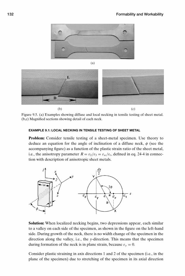
132 Formability and Workability
(a)
(b) (c)
Figure 9.5. (a) Examples showing diffuse and local necking in tensile testing of sheet metal.(b,c) Magnified sections showing detail of each neck.
EXAMPLE 9.1: LOCAL NECKING IN TENSILE TESTING OF SHEET METAL
Problem: Consider tensile testing of a sheet-metal specimen. Use theory todeduce an equation for the angle of inclination of a diffuse neck, φ (see theaccompanying figure) as a function of the plastic strain ratio of the sheet metal,i.e., the anisotropy parameter R = ε2/ε3 = εw/εt , defined in eq. 24-4 in connec-tion with description of anisotropic sheet metals.
Solution: When localized necking begins, two depressions appear, each similarto a valley on each side of the specimen, as shown in the figure on the left-handside. During growth of the neck, there is no width change of the specimen in thedirection along the valley, i.e., the y-direction. This means that the specimenduring formation of the neck is in plane strain, because εy = 0.
Consider plastic straining in axis directions 1 and 2 of the specimen (i.e., in theplane of the specimen) due to stretching of the specimen in its axial direction
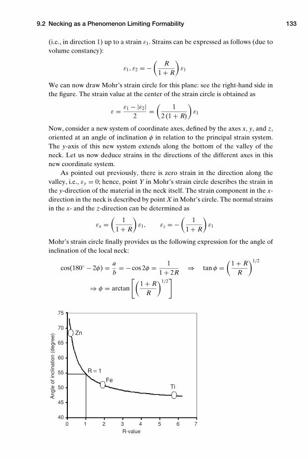
9.2 Necking as a Phenomenon Limiting Formability 133
(i.e., in direction 1) up to a strain ε1. Strains can be expressed as follows (due tovolume constancy):
ε1, ε2 = −(
R1 + R
)ε1
We can now draw Mohr’s strain circle for this plane: see the right-hand side inthe figure. The strain value at the center of the strain circle is obtained as
ε = ε1 − |ε2|2
=(
12 (1 + R)
)ε1
Now, consider a new system of coordinate axes, defined by the axes x, y, and z,oriented at an angle of inclination φ in relation to the principal strain system.The y-axis of this new system extends along the bottom of the valley of theneck. Let us now deduce strains in the directions of the different axes in thisnew coordinate system.
As pointed out previously, there is zero strain in the direction along thevalley, i.e., εy = 0; hence, point Y in Mohr’s strain circle describes the strain inthe y-direction of the material in the neck itself. The strain component in the x-direction in the neck is described by point X in Mohr’s circle. The normal strainsin the x- and the z-direction can be determined as
εx =(
11 + R
)ε1, εz = −
(1
1 + R
)ε1
Mohr’s strain circle finally provides us the following expression for the angle ofinclination of the local neck:
cos(180◦ − 2φ) = ab
= − cos 2φ = 11 + 2R
⇒ tan φ =(
1 + RR
)1/2
⇒ φ = arctan
[(1 + R
R
)1/2]
75
70
65
60
55
50
45
400 1 2 3 4 5 6 7
R-value
Ang
le o
f inc
linat
ion
(deg
ree)
Zn
R = 1
FeTi
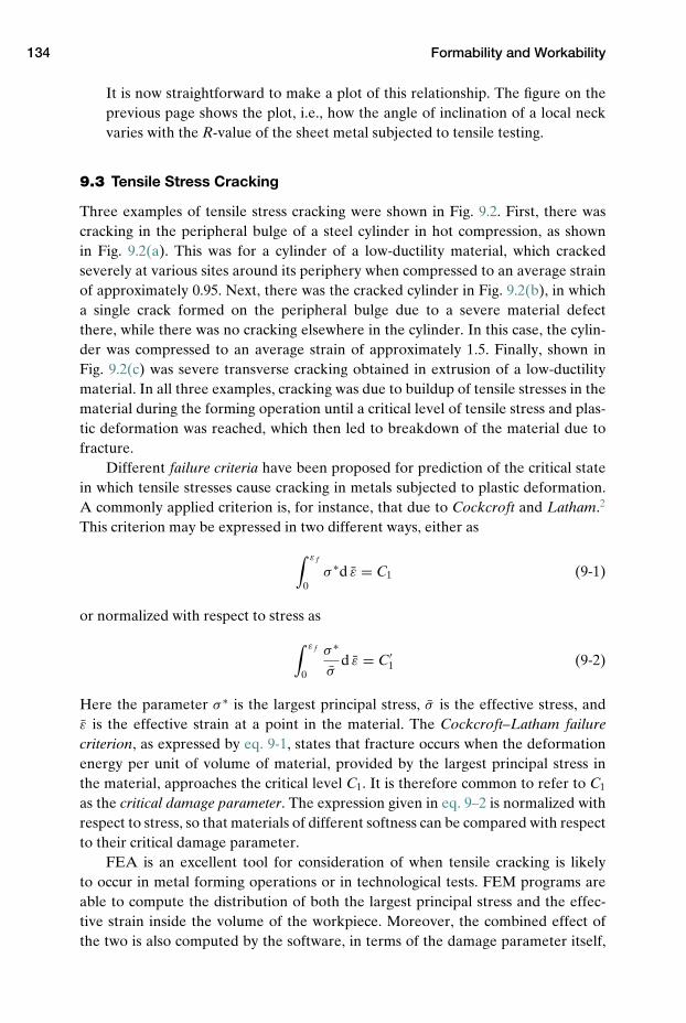
134 Formability and Workability
It is now straightforward to make a plot of this relationship. The figure on theprevious page shows the plot, i.e., how the angle of inclination of a local neckvaries with the R-value of the sheet metal subjected to tensile testing.
9.3 Tensile Stress Cracking
Three examples of tensile stress cracking were shown in Fig. 9.2. First, there wascracking in the peripheral bulge of a steel cylinder in hot compression, as shownin Fig. 9.2(a). This was for a cylinder of a low-ductility material, which crackedseverely at various sites around its periphery when compressed to an average strainof approximately 0.95. Next, there was the cracked cylinder in Fig. 9.2(b), in whicha single crack formed on the peripheral bulge due to a severe material defectthere, while there was no cracking elsewhere in the cylinder. In this case, the cylin-der was compressed to an average strain of approximately 1.5. Finally, shown inFig. 9.2(c) was severe transverse cracking obtained in extrusion of a low-ductilitymaterial. In all three examples, cracking was due to buildup of tensile stresses in thematerial during the forming operation until a critical level of tensile stress and plas-tic deformation was reached, which then led to breakdown of the material due tofracture.
Different failure criteria have been proposed for prediction of the critical statein which tensile stresses cause cracking in metals subjected to plastic deformation.A commonly applied criterion is, for instance, that due to Cockcroft and Latham.2
This criterion may be expressed in two different ways, either as
∫ ε f
0σ ∗d ε = C1 (9-1)
or normalized with respect to stress as
∫ ε f
0
σ ∗
σd ε = C′
1 (9-2)
Here the parameter σ ∗ is the largest principal stress, σ is the effective stress, andε is the effective strain at a point in the material. The Cockcroft–Latham failurecriterion, as expressed by eq. 9-1, states that fracture occurs when the deformationenergy per unit of volume of material, provided by the largest principal stress inthe material, approaches the critical level C1. It is therefore common to refer to C1
as the critical damage parameter. The expression given in eq. 9–2 is normalized withrespect to stress, so that materials of different softness can be compared with respectto their critical damage parameter.
FEA is an excellent tool for consideration of when tensile cracking is likelyto occur in metal forming operations or in technological tests. FEM programs areable to compute the distribution of both the largest principal stress and the effec-tive strain inside the volume of the workpiece. Moreover, the combined effect ofthe two is also computed by the software, in terms of the damage parameter itself,
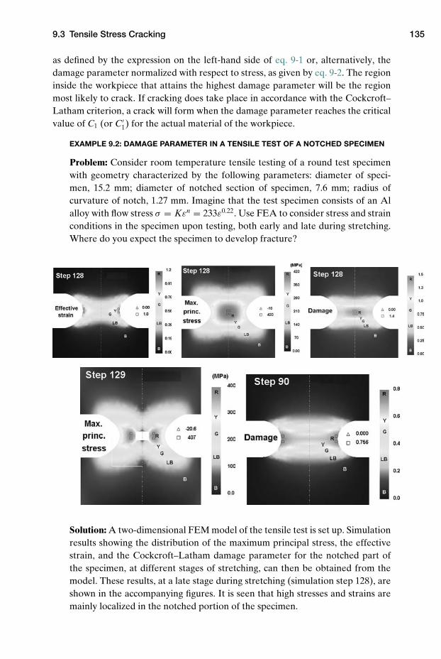
9.3 Tensile Stress Cracking 135
as defined by the expression on the left-hand side of eq. 9-1 or, alternatively, thedamage parameter normalized with respect to stress, as given by eq. 9-2. The regioninside the workpiece that attains the highest damage parameter will be the regionmost likely to crack. If cracking does take place in accordance with the Cockcroft–Latham criterion, a crack will form when the damage parameter reaches the criticalvalue of C1 (or C′
1) for the actual material of the workpiece.
EXAMPLE 9.2: DAMAGE PARAMETER IN A TENSILE TEST OF A NOTCHED SPECIMEN
Problem: Consider room temperature tensile testing of a round test specimenwith geometry characterized by the following parameters: diameter of speci-men, 15.2 mm; diameter of notched section of specimen, 7.6 mm; radius ofcurvature of notch, 1.27 mm. Imagine that the test specimen consists of an Alalloy with flow stress σ = Kεn = 233ε0.22. Use FEA to consider stress and strainconditions in the specimen upon testing, both early and late during stretching.Where do you expect the specimen to develop fracture?
Solution: A two-dimensional FEM model of the tensile test is set up. Simulationresults showing the distribution of the maximum principal stress, the effectivestrain, and the Cockcroft–Latham damage parameter for the notched part ofthe specimen, at different stages of stretching, can then be obtained from themodel. These results, at a late stage during stretching (simulation step 128), areshown in the accompanying figures. It is seen that high stresses and strains aremainly localized in the notched portion of the specimen.
136 Formability and Workability
The effective strain, shown in the upper left picture, is highest on the surface ofthe specimen, just below the notch. The principal stress, which is tensile, however,is highest at the center of the notch of the specimen (upper middle picture). Finally,as shown on the upper right, the highest damage parameter during this late stageof stretching is predicted to appear right at the center of the notched part of thespecimen. Hence, from the simulation results, we can conclude that late during thecourse of stretching, cracking due to buildup of tensile stress most likely will occurat the center of the specimen.
A simulation of crack formation in the specimen under these circumstances isshown in the figure on the lower left. The picture depicts by its principal stress distri-bution that, after initiation of a crack at the center of the specimen, tensile stressesremain high ahead of the crack tip. This causes further crack growth, until full frac-ture has been realized over the whole notched cross section.
On the lower right in the figure, the FEM-predicted distribution of the dam-age parameter is shown as it appears early during testing, i.e., at simulation step 90.The critical region inside the specimen as regards the damage parameter is now inthe surface layer of the specimen, below the surface of the notch. These results indi-cate that whereas a low-ductility material in the notch would tend to develop surfacecracks, a high ductility material would be most prone to fail by center cracking there.
9.3.1 Tensile Stress Cracking in Cylinder Compression
As shown in Fig. 9.2(a), cracking may occur in the bulged portion of a cylinder. Formaterial of good ductility, this is the most likely site for crack formation.
Figure 9.6 shows results from FEM simulation of cylinder compression. Thehighest damage parameter is predicted to occur in the middle of the bulge. This loca-tion is therefore the most likely site for crack initiation. The high damage parameterhere is caused by the high tensile stresses acting in the direction around the circum-ference of the cylinder, [see Fig. 9.6(b)]; the deformations at this location are notespecially large [see Fig. 9.6(c)].
9.4 Shear Cracking in the Cylinder Compression Test
In Fig. 9.3(a) and (b) an example was shown where shear cracking occurred in coldcylinder compression. The material of the cylinder used in this experiment wasan AA 7108 alloy in as-extruded condition. Compression testing of the materialrevealed that the flow curve of this material was one characterized by strain-inducedsoftening; see Fig. 9.7(a).
FEA results mimicking this cylinder compression process are shown inFig. 9.7(b). The analysis reveals the well-known fact that a deformation shear crossforms inside the cylinder when there is friction between the die and the cylinder. Thelargest deformations will appear in the shear cross. When the cylinder has been com-pressed down to a certain stage, the initial strain-hardening part of the flow curvehas been exceeded for the material in the shear layer. With continued compression,
9.4 Shear Cracking in the Cylinder Compression Test 137
(a)
(b) (c)
Figure 9.6. FEM-simulation results showing (a) high damage parameter in the bulge of thecylinder, (b) high tensile stress over the circumference of the bulge, and (c) moderate effectivestrain in the bulge.
(a) (b)
Figure 9.7. (a) Flow curve for material that exhibits strain softening. (b) FEA depicting highstrain at shear plane, which fails by fracture in the experiment shown in Fig. 9.3(a) and (b).
138 Formability and Workability
the shear layer will then experience strain-induced softening. Deformations thenwill tend to localize in a thin layer, as marked with the broken line in this figure.Because of strain softening, this layer will then easily become overstrained, and ashear fracture will form here.
In cylinder compression, the shear cross appears three-dimensionally with acomplex shape similar to an hourglass. Even though the shear fracture is initiatedsomewhere along the plane of the shear cross, propagation of the fracture duringfurther growth most commonly follows a plane path, so that a plane fracture surfaceis obtained. Upon cracking, a bit of the material may be detached from the rest ofthe cylinder; see Fig. 9.3(b).
Problem
9.1 In the accompanying figure, a FEM record of largest tensile stress vs. effectivestrain is shown for a material point in a tensile test specimen with a notch. Thematerial point for which the data were attained was located in the middle of thenotched part of the specimen. Estimate the Cockcroft–Latham damage parameter,eq. 9-1, for this material point for an effective strain value of 0.4 and 0.7.
600
400
200
00 0.2 0.4 0.6 0.8
Effective strain
Larg
est p
rinci
pal
stre
ss (
MP
a)
NOTES
1. Mielnik, E. M.: “Metalworking Science and Engineering,” McGraw-Hill, New York,1991, p. 494.
2. Cockcroft, M. C., and Latham, D. J.: “Ductility and workability of metals,” J. Inst. ofMetals, Vol. 96, 1968, pp. 33–39.
REFERENCES
Bunge, H. J., Pohlandt, K., and Tekkaya, A. E.: “Formability of Metallic Materials: PlasticAnisotropy, Formability Testing, Forming Limits,” Springer Verlag, 2000.
Dieter, G. E., Kuhn, H. A., and Semiatin, S. L.: “Handbook of Workability and ProcessDesign,” ASM Int., 2003.
Mielnik, E. M.: “Metalworking Science and Engineering,” McGraw-Hill, New York, 1991.Semiatin, S. L., and Jonas, J. J.: “Formability and Workability of Metals,” ASM Int., 1984.Wright, T. W.: “The Physics and Mathematics of Adiabatic Shear Bands,” Cambridge Univ.
Press, 2002.
10 Friction and Friction Models
In metal forming, friction is a crucial factor that determines whether an industrialprocess can be run with acceptable, economic result. In many forming applications,the actual friction conditions are not sufficiently known. In spite of much researchon that important topic, there is still lack of knowledge and need for continuedresearch.
This chapter will first explain why friction is so important in metal forming.Then the two most-applied friction models will be presented, and the characteristicof each model will be explained and discussed. Afterwards the most common lubri-cation mechanisms that may be present in the interface between die and workpiecewill be described. Moreover, it will be explained how relevant metal forming fric-tion data can be measured by the ring compression test. Finally, it will be shownhow in situ friction measurements can be performed inside a die during the courseof forming, using pins inserted into holes drilled into the tooling.
10.1 Friction Effects in Metal Forming
The friction phenomenon in metal forming is of great importance. There are variousreasons for this:
� Forming loads and stresses transferred to the dies depend on friction and canbe reduced by use of appropriate lubricants.
� The surface quality of the formed workpiece depends on the lubricant used.If there is lubricant breakdown during forming, the product may obtain badsurface quality (for instance, scoring).
� Wear of the dies can be reduced if lubricant films are applied, which providereduced friction, or even full or partial separation, between the die and theworkpiece during forming.
An important reason why friction in metal forming is not fully understood yet isthat it is very difficult to enter into the boundary interface between the workpieceand the die, to make in situ observations of what takes place there. Most commonlyit is also difficult to measure friction, because the friction shear stress transferred
139
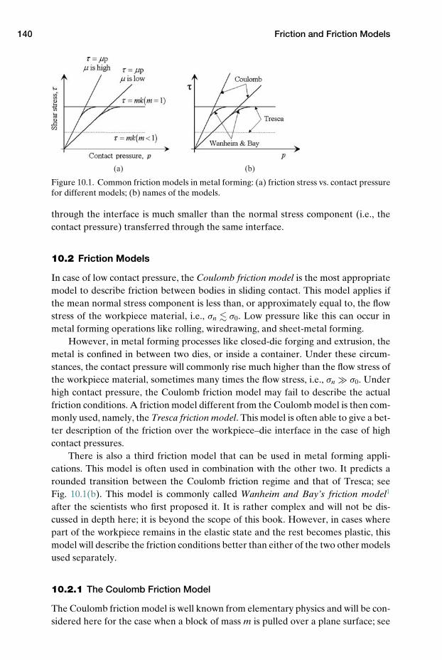
140 Friction and Friction Models
(a) (b)
Figure 10.1. Common friction models in metal forming: (a) friction stress vs. contact pressurefor different models; (b) names of the models.
through the interface is much smaller than the normal stress component (i.e., thecontact pressure) transferred through the same interface.
10.2 Friction Models
In case of low contact pressure, the Coulomb friction model is the most appropriatemodel to describe friction between bodies in sliding contact. This model applies ifthe mean normal stress component is less than, or approximately equal to, the flowstress of the workpiece material, i.e., σn � σ0. Low pressure like this can occur inmetal forming operations like rolling, wiredrawing, and sheet-metal forming.
However, in metal forming processes like closed-die forging and extrusion, themetal is confined in between two dies, or inside a container. Under these circum-stances, the contact pressure will commonly rise much higher than the flow stress ofthe workpiece material, sometimes many times the flow stress, i.e., σn σ0. Underhigh contact pressure, the Coulomb friction model may fail to describe the actualfriction conditions. A friction model different from the Coulomb model is then com-monly used, namely, the Tresca friction model. This model is often able to give a bet-ter description of the friction over the workpiece–die interface in the case of highcontact pressures.
There is also a third friction model that can be used in metal forming appli-cations. This model is often used in combination with the other two. It predicts arounded transition between the Coulomb friction regime and that of Tresca; seeFig. 10.1(b). This model is commonly called Wanheim and Bay’s friction model1
after the scientists who first proposed it. It is rather complex and will not be dis-cussed in depth here; it is beyond the scope of this book. However, in cases wherepart of the workpiece remains in the elastic state and the rest becomes plastic, thismodel will describe the friction conditions better than either of the two other modelsused separately.
10.2.1 The Coulomb Friction Model
The Coulomb friction model is well known from elementary physics and will be con-sidered here for the case when a block of mass m is pulled over a plane surface; see
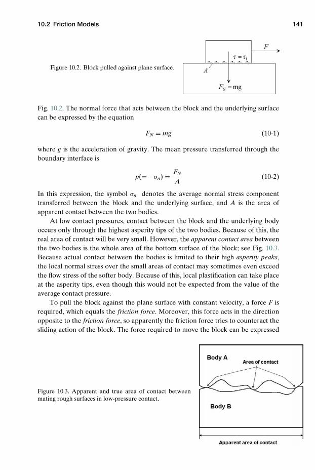
10.2 Friction Models 141
Figure 10.2. Block pulled against plane surface.
Fig. 10.2. The normal force that acts between the block and the underlying surfacecan be expressed by the equation
FN = mg (10-1)
where g is the acceleration of gravity. The mean pressure transferred through theboundary interface is
p(= −σn) = FN
A(10-2)
In this expression, the symbol σn denotes the average normal stress componenttransferred between the block and the underlying surface, and A is the area ofapparent contact between the two bodies.
At low contact pressures, contact between the block and the underlying bodyoccurs only through the highest asperity tips of the two bodies. Because of this, thereal area of contact will be very small. However, the apparent contact area betweenthe two bodies is the whole area of the bottom surface of the block; see Fig. 10.3.Because actual contact between the bodies is limited to their high asperity peaks,the local normal stress over the small areas of contact may sometimes even exceedthe flow stress of the softer body. Because of this, local plastification can take placeat the asperity tips, even though this would not be expected from the value of theaverage contact pressure.
To pull the block against the plane surface with constant velocity, a force F isrequired, which equals the friction force. Moreover, this force acts in the directionopposite to the friction force, so apparently the friction force tries to counteract thesliding action of the block. The force required to move the block can be expressed
Figure 10.3. Apparent and true area of contact betweenmating rough surfaces in low-pressure contact.
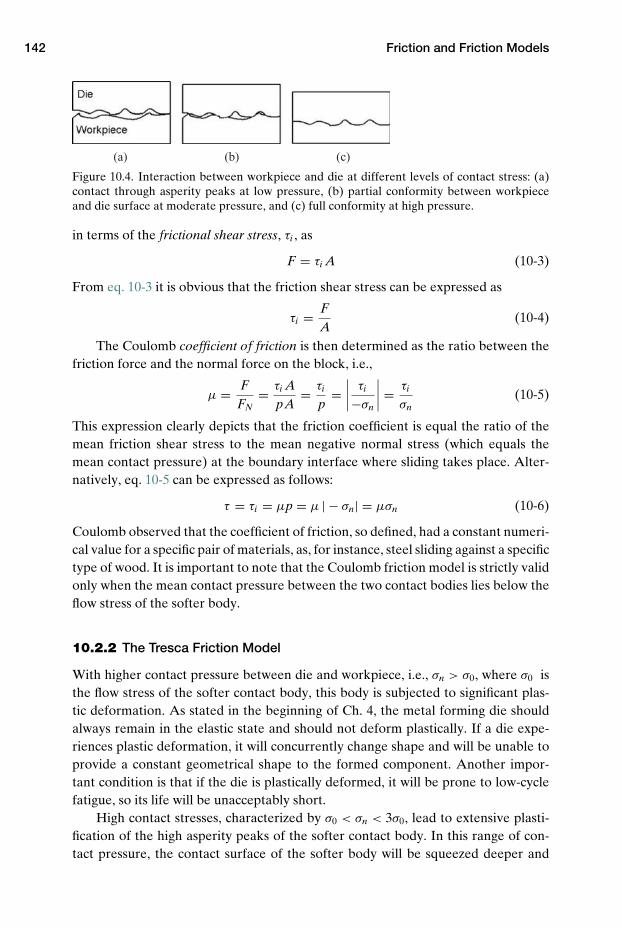
142 Friction and Friction Models
(a) (b) (c)
Figure 10.4. Interaction between workpiece and die at different levels of contact stress: (a)contact through asperity peaks at low pressure, (b) partial conformity between workpieceand die surface at moderate pressure, and (c) full conformity at high pressure.
in terms of the frictional shear stress, τi , as
F = τi A (10-3)
From eq. 10-3 it is obvious that the friction shear stress can be expressed as
τi = FA
(10-4)
The Coulomb coefficient of friction is then determined as the ratio between thefriction force and the normal force on the block, i.e.,
µ = FFN
= τi ApA
= τi
p=
∣∣∣∣ τi
−σn
∣∣∣∣ = τi
σn(10-5)
This expression clearly depicts that the friction coefficient is equal the ratio of themean friction shear stress to the mean negative normal stress (which equals themean contact pressure) at the boundary interface where sliding takes place. Alter-natively, eq. 10-5 can be expressed as follows:
τ = τi = µp = µ | − σn| = µσn (10-6)
Coulomb observed that the coefficient of friction, so defined, had a constant numeri-cal value for a specific pair of materials, as, for instance, steel sliding against a specifictype of wood. It is important to note that the Coulomb friction model is strictly validonly when the mean contact pressure between the two contact bodies lies below theflow stress of the softer body.
10.2.2 The Tresca Friction Model
With higher contact pressure between die and workpiece, i.e., σn > σ0, where σ0 isthe flow stress of the softer contact body, this body is subjected to significant plas-tic deformation. As stated in the beginning of Ch. 4, the metal forming die shouldalways remain in the elastic state and should not deform plastically. If a die expe-riences plastic deformation, it will concurrently change shape and will be unable toprovide a constant geometrical shape to the formed component. Another impor-tant condition is that if the die is plastically deformed, it will be prone to low-cyclefatigue, so its life will be unacceptably short.
High contact stresses, characterized by σ0 < σn < 3σ0, lead to extensive plasti-fication of the high asperity peaks of the softer contact body. In this range of con-tact pressure, the contact surface of the softer body will be squeezed deeper and
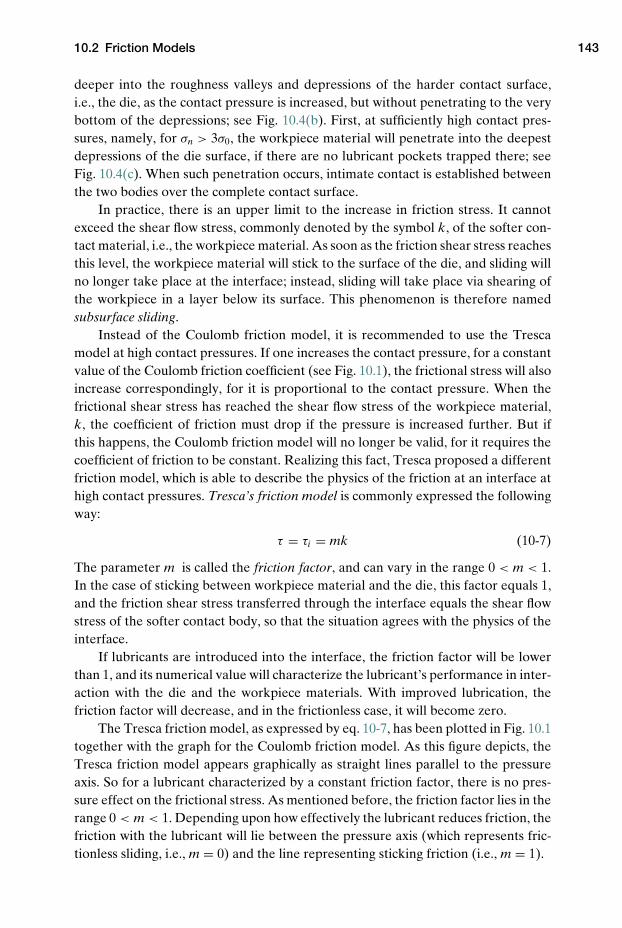
10.2 Friction Models 143
deeper into the roughness valleys and depressions of the harder contact surface,i.e., the die, as the contact pressure is increased, but without penetrating to the verybottom of the depressions; see Fig. 10.4(b). First, at sufficiently high contact pres-sures, namely, for σn > 3σ0, the workpiece material will penetrate into the deepestdepressions of the die surface, if there are no lubricant pockets trapped there; seeFig. 10.4(c). When such penetration occurs, intimate contact is established betweenthe two bodies over the complete contact surface.
In practice, there is an upper limit to the increase in friction stress. It cannotexceed the shear flow stress, commonly denoted by the symbol k, of the softer con-tact material, i.e., the workpiece material. As soon as the friction shear stress reachesthis level, the workpiece material will stick to the surface of the die, and sliding willno longer take place at the interface; instead, sliding will take place via shearing ofthe workpiece in a layer below its surface. This phenomenon is therefore namedsubsurface sliding.
Instead of the Coulomb friction model, it is recommended to use the Trescamodel at high contact pressures. If one increases the contact pressure, for a constantvalue of the Coulomb friction coefficient (see Fig. 10.1), the frictional stress will alsoincrease correspondingly, for it is proportional to the contact pressure. When thefrictional shear stress has reached the shear flow stress of the workpiece material,k, the coefficient of friction must drop if the pressure is increased further. But ifthis happens, the Coulomb friction model will no longer be valid, for it requires thecoefficient of friction to be constant. Realizing this fact, Tresca proposed a differentfriction model, which is able to describe the physics of the friction at an interface athigh contact pressures. Tresca’s friction model is commonly expressed the followingway:
τ = τi = mk (10-7)
The parameter m is called the friction factor, and can vary in the range 0 < m < 1.In the case of sticking between workpiece material and the die, this factor equals 1,and the friction shear stress transferred through the interface equals the shear flowstress of the softer contact body, so that the situation agrees with the physics of theinterface.
If lubricants are introduced into the interface, the friction factor will be lowerthan 1, and its numerical value will characterize the lubricant’s performance in inter-action with the die and the workpiece materials. With improved lubrication, thefriction factor will decrease, and in the frictionless case, it will become zero.
The Tresca friction model, as expressed by eq. 10-7, has been plotted in Fig. 10.1together with the graph for the Coulomb friction model. As this figure depicts, theTresca friction model appears graphically as straight lines parallel to the pressureaxis. So for a lubricant characterized by a constant friction factor, there is no pres-sure effect on the frictional stress. As mentioned before, the friction factor lies in therange 0 < m < 1. Depending upon how effectively the lubricant reduces friction, thefriction with the lubricant will lie between the pressure axis (which represents fric-tionless sliding, i.e., m = 0) and the line representing sticking friction (i.e., m = 1).
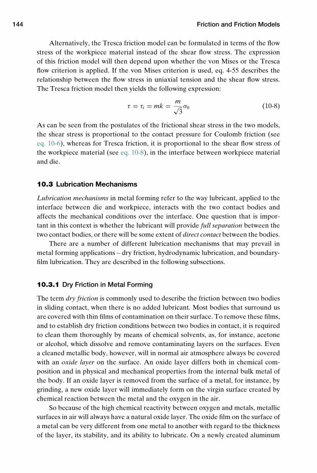
144 Friction and Friction Models
Alternatively, the Tresca friction model can be formulated in terms of the flowstress of the workpiece material instead of the shear flow stress. The expressionof this friction model will then depend upon whether the von Mises or the Trescaflow criterion is applied. If the von Mises criterion is used, eq. 4-55 describes therelationship between the flow stress in uniaxial tension and the shear flow stress.The Tresca friction model then yields the following expression:
τ = τi = mk = m√3σ0 (10-8)
As can be seen from the postulates of the frictional shear stress in the two models,the shear stress is proportional to the contact pressure for Coulomb friction (seeeq. 10-6), whereas for Tresca friction, it is proportional to the shear flow stress ofthe workpiece material (see eq. 10-8), in the interface between workpiece materialand die.
10.3 Lubrication Mechanisms
Lubrication mechanisms in metal forming refer to the way lubricant, applied to theinterface between die and workpiece, interacts with the two contact bodies andaffects the mechanical conditions over the interface. One question that is impor-tant in this context is whether the lubricant will provide full separation between thetwo contact bodies, or there will be some extent of direct contact between the bodies.
There are a number of different lubrication mechanisms that may prevail inmetal forming applications – dry friction, hydrodynamic lubrication, and boundary-film lubrication. They are described in the following subsections.
10.3.1 Dry Friction in Metal Forming
The term dry friction is commonly used to describe the friction between two bodiesin sliding contact, when there is no added lubricant. Most bodies that surround usare covered with thin films of contamination on their surface. To remove these films,and to establish dry friction conditions between two bodies in contact, it is requiredto clean them thoroughly by means of chemical solvents, as, for instance, acetoneor alcohol, which dissolve and remove contaminating layers on the surfaces. Evena cleaned metallic body, however, will in normal air atmosphere always be coveredwith an oxide layer on the surface. An oxide layer differs both in chemical com-position and in physical and mechanical properties from the internal bulk metal ofthe body. If an oxide layer is removed from the surface of a metal, for instance, bygrinding, a new oxide layer will immediately form on the virgin surface created bychemical reaction between the metal and the oxygen in the air.
So because of the high chemical reactivity between oxygen and metals, metallicsurfaces in air will always have a natural oxide layer. The oxide film on the surface ofa metal can be very different from one metal to another with regard to the thicknessof the layer, its stability, and its ability to lubricate. On a newly created aluminum

10.3 Lubrication Mechanisms 145
(a) (b)
Figure 10.5. In dry friction compression of a cylinder of Althere is (a) sticking friction; for Cu there is (b) sliding friction.
surface, for instance, a thin, adhering film of Al2O3 will immediately form. This filmis dense and protects the underlying metal from further chemical reaction with thesurrounding air. Copper, brass, and steel surfaces likewise form chemical reactionfilms, but these films are less dense and, therefore, less stable, so they will usuallygrow in thickness over time. The growth conditions of such films will be stronglyinfluenced by the presence of water or corrosive liquids on the surface considered,as well as the temperature.
Because oxide layers normally cover metallic surfaces, the dry friction behaviorof different metals may vary a lot. When a workpiece establishes contact with adie, the natural oxide films on the surfaces of both bodies will appear as films inthe interface between the bodies. Dry friction contact conditions usually dependstrongly on whether the films are able to lubricate the contact surface.
The difference in behavior of the end surface of a cylinder of Al and one of Cuin nonlubricated compression, i.e., in the case of dry friction, illustrates clearly (seeFig. 10.5), to what extent oxide layers can lubricate an interface. If the cylinders ofthe two metals are well cleaned before compression, the Al cylinder will stick com-pletely to the die surface, whereas for the Cu cylinder there will be sliding friction.The different behavior can be shown by use of a stripe of marker material in thecylinder, obtained by inserting a contrast pin into the cylinder, as explained in Ch.12. Then for the cylinder of Al, the stripe will remain in the same position on theinterface before and after compression [see arrows in Fig. 10.5(a)], and hence willdocument sticking friction. In contrast, for the Cu cylinder there will be sliding fric-tion [see arrows in Fig. 10.5(b)]. As a consequence of this, during compression thestripe will flow outward in the radial direction at the die–cylinder interface.
The difference in metal flow during dry friction compression of the two cylin-ders in the experiments mentioned is caused by the different properties of the oxidelayers on the surfaces of the two metals. Al has a dense adherent oxide layer on thesurface that does not lubricate the interface, and sliding will therefore not take placein this layer. On the other hand, Cu has a porous oxide layer of low shear strengththat acts as a lubricant and reduces friction. Because of this, the material particleson the surface of the Cu cylinder will slide along the interface, instead of remainingin the same position during the compression stroke as they do for an Al cylinder.
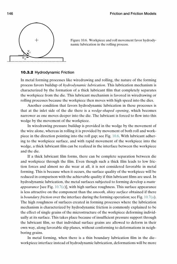
146 Friction and Friction Models
Figure 10.6. Workpiece and roll movement favor hydrody-namic lubrication in the rolling process.
10.3.2 Hydrodynamic Friction
In metal forming processes like wiredrawing and rolling, the nature of the formingprocess favors buildup of hydrodynamic lubrication. This lubrication mechanism ischaracterized by the formation of a thick lubricant film that completely separatesthe workpiece from the die. This lubricant mechanism is favored in wiredrawing orrolling processes because the workpiece then moves with high speed into the dies.
Another condition that favors hydrodynamic lubrication in these processes isthat at the inlet side of the die there is a wedge-shaped opening, which becomesnarrower as one moves deeper into the die. The lubricant is forced to flow into thiswedge by the movement of the workpiece.
In wiredrawing pressure buildup is provided in the wedge by the movement ofthe wire alone, whereas in rolling it is provided by movement of both roll and work-piece in the direction pointing into the roll gap; see Fig. 10.6. With lubricant adher-ing to the workpiece surface, and with rapid movement of the workpiece into thewedge, a thick lubricant film can be realized in the interface between the workpieceand the die.
If a thick lubricant film forms, there can be complete separation between dieand workpiece through the film. Even though such a thick film leads to low fric-tion forces and almost no die wear at all, it is not considered favorable in metalforming. This is because when it occurs, the surface quality of the workpiece will bereduced in comparison with the achievable quality if thin lubricant films are used. Inhydrodynamic lubrication, the metal surfaces subjected to forming develop a matteappearance [see Fig. 10.7(c)], with high surface roughness. This surface appearanceis less attractive on the component than the smooth, shiny surface obtained if thereis boundary friction over the interface during the forming operation; see Fig. 10.7(a).The high roughness of surfaces created in forming processes where the lubricationmechanism is characterized by hydrodynamic friction is commonly explained to bethe effect of single grains of the microstructure of the workpiece deforming individ-ually at its surface. This takes place because of insufficient pressure support throughthe lubricant film, so that individual surface grains are allowed to deform in theirown way, along favorable slip planes, without conforming to deformations in neigh-boring grains.
In metal forming, when there is a thin boundary lubrication film in the die–workpiece interface instead of hydrodynamic lubrication, deformations will be more

10.3 Lubrication Mechanisms 147
0.1 mm
(a) (b) (c)
Figure 10.7. Surface appearance (magnified) of surfaces produced in rolling2 processesby (a) boundary layer lubrication, (b) breakdown of lubricant film, and (c) hydrody-namic lubrication (reprinted with permission of ASM International. All rights reserved.www.asminternational.org).
evenly distributed throughout the volume of the surface grains, and a smoother,brighter surface appearance will result.
From this it is obvious that the main factor favoring formation of hydrody-namic lubrication in metal forming processes like rolling and drawing is high form-ing velocity. The lubricant is then forced with high speed into the wedge-shapedopening at the inlet side of the plastic zone, so that a high lubrication pressure buildsup there. With increased lubricant supply into the wedge, lubricant penetration intothe interface between the two contact bodies is eased, and hence lubrication willbe improved. Another process parameter of great importance is the viscosity of thelubricant. Higher viscosity will lead to higher pressure buildup in the wedge at theinlet side of the deformation gap, where forming takes place. Because of this, lubri-cants with high viscosity favor the formation of hydrodynamic lubrication films.
When the lubrication mechanism is hydrodynamic, friction is low. This isbecause the shear stresses transferred through the interface between the two con-tact bodies depend on the shear properties of the lubricant film only, as there is nolonger direct contact between the surface asperities of the two bodies. In the case ofhydrodynamic friction, the coefficient of friction can therefore be as low as µ < 0.01.
10.3.3 Boundary Film Lubrication
It is generally claimed that the most favorable lubrication condition in metal formingis boundary film lubrication. When this lubrication mechanism prevails, a thin – andvery effective – lubricant film persists in the interface between workpiece and die.Boundary film lubrication is able to provide rather complete separation betweenthe two contact bodies; see Fig. 10.8(a). The thickness of the lubricant film in thiscase is typically of the same magnitude as the average length of the chain moleculesof the lubricant. In this case, relatively high stresses can be transferred across thefilm, and through the contact interface, without damaging the film. In boundary filmlubrication, each surface grain of the microstructure of the workpiece will be forced
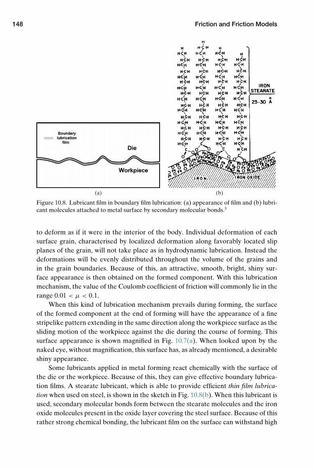
148 Friction and Friction Models
(a) (b)
Figure 10.8. Lubricant film in boundary film lubrication: (a) appearance of film and (b) lubri-cant molecules attached to metal surface by secondary molecular bonds.3
to deform as if it were in the interior of the body. Individual deformation of eachsurface grain, characterised by localized deformation along favorably located slipplanes of the grain, will not take place as in hydrodynamic lubrication. Instead thedeformations will be evenly distributed throughout the volume of the grains andin the grain boundaries. Because of this, an attractive, smooth, bright, shiny sur-face appearance is then obtained on the formed component. With this lubricationmechanism, the value of the Coulomb coefficient of friction will commonly lie in therange 0.01 < µ < 0.1.
When this kind of lubrication mechanism prevails during forming, the surfaceof the formed component at the end of forming will have the appearance of a finestripelike pattern extending in the same direction along the workpiece surface as thesliding motion of the workpiece against the die during the course of forming. Thissurface appearance is shown magnified in Fig. 10.7(a). When looked upon by thenaked eye, without magnification, this surface has, as already mentioned, a desirableshiny appearance.
Some lubricants applied in metal forming react chemically with the surface ofthe die or the workpiece. Because of this, they can give effective boundary lubrica-tion films. A stearate lubricant, which is able to provide efficient thin film lubrica-tion when used on steel, is shown in the sketch in Fig. 10.8(b). When this lubricant isused, secondary molecular bonds form between the stearate molecules and the ironoxide molecules present in the oxide layer covering the steel surface. Because of thisrather strong chemical bonding, the lubricant film on the surface can withstand high
10.4 Measurement of Friction in Metal Forming 149
shear stresses due to friction without being torn away from the surface. The thinfilm formed this way adheres firmly to the surface that it is bonded to and hence canprovide efficient boundary film lubrication in metal forming.
In practical cases of metal forming, it is quite common to have boundary filmlubrication combined with metallic contact at local spots on the die surface, i.e., amixed lubrication mechanism. For this kind of contact, the Coulomb coefficient offriction is commonly claimed to lie in the range µ = 0.1–0.3.
In some situations, there may be local breakdown of the lubricant film in spotsalong the boundary interface between die and workpiece. In contrast to boundaryfilm lubrication, the workpiece surface may then obtain an unattractive, speckled,appearance, such as that shown in Fig. 10.7(b).
10.4 Measurement of Friction in Metal Forming
Although it is commonly straightforward to measure friction in general non-metal-forming situations encountered in everyday life, this is not the case when it comesto friction in metal forming. In metal forming, the most commonly used method ofmeasuring friction is perhaps the ring compression test. This test method will there-fore be described in detail.
An alternative method for measurement of friction in metal forming is by use ofpins inserted into the die. A pair of holes is first drilled through the tooling, wheresteel pins, which consist of a material the same as or similar to the die material,are inserted into the holes. The end face of the pins must be flush with the die sur-face during the measurement. Each pin is fitted with a sensor at its rear end, insidethe tooling. The force transferred to each pin from the workpiece material at theinterface with the die can be read out by means of this sensor. In this way, the con-tact stress, both normal and shear, at a point on the contact surface can be obtainedfrom primary force measurements. When the stresses have been determined, it isstraightforward to compute the local friction value on the interface where the mea-surement was performed. Various aspects of use of pins on the die or workpiece forfriction measurement will be discussed in the further treatment here.
Strip drawing4 is a metal forming process in which the average friction on thedrawing die can be determined directly from measurement of the die splitting forceand the drawing force. It will not be treated here, being beyond the scope of thisbook.
10.4.1 Metal Forming Friction from Ring Compression
In metal forming, it is common to apply the ring compression test5 to determinefriction in situations where metallic bodies are subjected to plastic deformationsagainst die surfaces. This technique was developed quite early, and in most cases, itwill provide reasonable friction values for a selected material pair (workpiece anddie material), either in dry friction or in interaction with a particular lubricant.
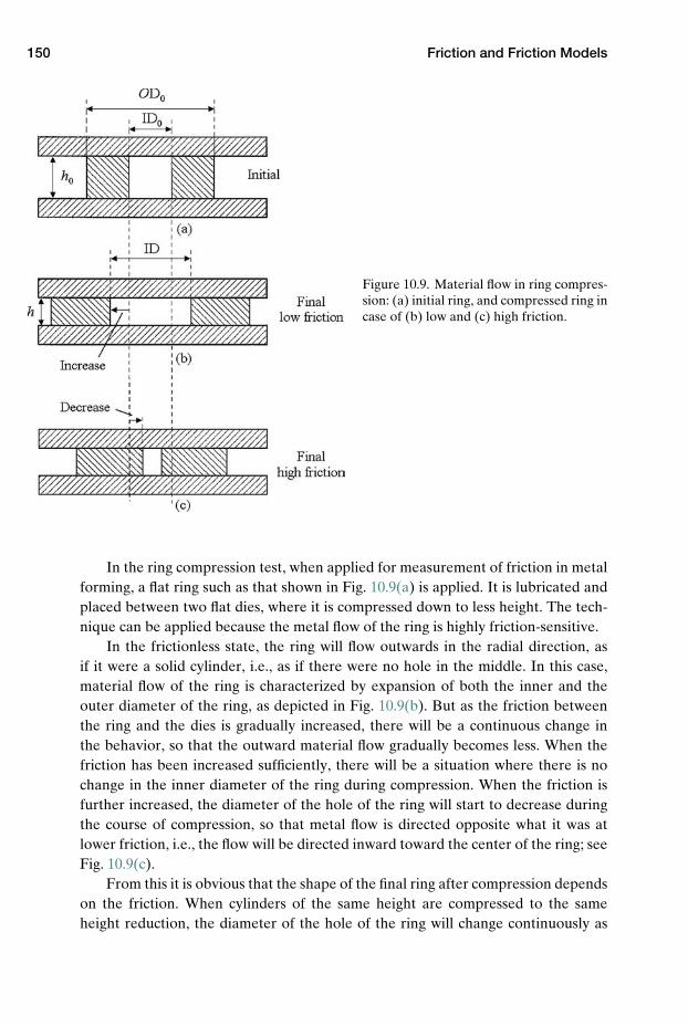
150 Friction and Friction Models
Figure 10.9. Material flow in ring compres-sion: (a) initial ring, and compressed ring incase of (b) low and (c) high friction.
In the ring compression test, when applied for measurement of friction in metalforming, a flat ring such as that shown in Fig. 10.9(a) is applied. It is lubricated andplaced between two flat dies, where it is compressed down to less height. The tech-nique can be applied because the metal flow of the ring is highly friction-sensitive.
In the frictionless state, the ring will flow outwards in the radial direction, asif it were a solid cylinder, i.e., as if there were no hole in the middle. In this case,material flow of the ring is characterized by expansion of both the inner and theouter diameter of the ring, as depicted in Fig. 10.9(b). But as the friction betweenthe ring and the dies is gradually increased, there will be a continuous change inthe behavior, so that the outward material flow gradually becomes less. When thefriction has been increased sufficiently, there will be a situation where there is nochange in the inner diameter of the ring during compression. When the friction isfurther increased, the diameter of the hole of the ring will start to decrease duringthe course of compression, so that metal flow is directed opposite what it was atlower friction, i.e., the flow will be directed inward toward the center of the ring; seeFig. 10.9(c).
From this it is obvious that the shape of the final ring after compression dependson the friction. When cylinders of the same height are compressed to the sameheight reduction, the diameter of the hole of the ring will change continuously as
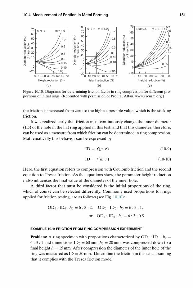
10.4 Measurement of Friction in Metal Forming 151
70
60
50
40
30
20
10
0
−10
80
70
60
50
40
30
20
10
0
−10
−20
70
60
50
40
30
20
10
0
−10
−20
100 20 30 40
(a) (b) (c)
50 60 70 100 20 30 40 50 60 70 100 20 30 40 50 60
Height reduction (%)Height reduction (%)Height reduction (%)
Dia
met
er r
educ
tion
(%)
of in
ner
hole
Dia
met
er r
educ
tion
(%)
of in
ner
hole
Dia
met
er r
educ
tion
(%)
of in
ner
hole
6 : 3 : 2 m = 1.06 : 3 : 1 m = 1.0 6 : 3 : 0.5 m = 1.0
0.7
0.5
0.3
0.20.15
0.100.05
0.7
0.5
0
0.3
0.20.15
0.10
0.05
0.70.5
0.3
0.2
0.15
0.10
0.05
Figure 10.10. Diagrams for determining friction factor in ring compression for different pro-portions of initial rings. (Reprinted with permission of Prof. T. Altan. www.ercnsm.org.)
the friction is increased from zero to the highest possible value, which is the stickingfriction.
It was realized early that friction must continuously change the inner diameter(ID) of the hole in the flat ring applied in this test, and that this diameter, therefore,can be used as a measure from which friction can be determined in ring compression.Mathematically this behavior can be expressed by
ID = f (µ, r) (10-9)
ID = f (m, r) (10-10)
Here, the first equation refers to compression with Coulomb friction and the secondequation to Tresca friction. As the equations show, the parameter height reductionr also influences the final value of the diameter of the inner hole.
A third factor that must be considered is the initial proportions of the ring,which of course can be selected differently. Commonly used proportions for ringsapplied for friction testing, are as follows (see Fig. 10.10):
OD0 : ID0 : h0 = 6 : 3 : 2, OD0 : ID0 : h0 = 6 : 3 : 1,
or OD0 : ID0 : h0 = 6 : 3 : 0.5
EXAMPLE 10.1: FRICTION FROM RING COMPRESSION EXPERIMENT
Problem: A ring specimen with proportions characterized by OD0 : ID0 : h0 =6 : 3 : 1 and dimensions ID0 = 60 mm, h0 = 20 mm, was compressed down to afinal height h = 15 mm. After compression the diameter of the inner hole of thering was measured as ID = 50 mm. Determine the friction in this test, assumingthat it complies with the Tresca friction model.
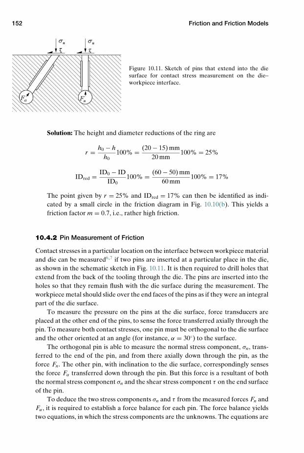
152 Friction and Friction Models
Figure 10.11. Sketch of pins that extend into the diesurface for contact stress measurement on the die–workpiece interface.
Solution: The height and diameter reductions of the ring are
r = h0 − hh0
100% = (20 − 15) mm20 mm
100% = 25%
IDred = ID0 − IDID0
100% = (60 − 50) mm60 mm
100% = 17%
The point given by r = 25% and IDred = 17% can then be identified as indi-cated by a small circle in the friction diagram in Fig. 10.10(b). This yields afriction factor m = 0.7, i.e., rather high friction.
10.4.2 Pin Measurement of Friction
Contact stresses in a particular location on the interface between workpiece materialand die can be measured6,7 if two pins are inserted at a particular place in the die,as shown in the schematic sketch in Fig. 10.11. It is then required to drill holes thatextend from the back of the tooling through the die. The pins are inserted into theholes so that they remain flush with the die surface during the measurement. Theworkpiece metal should slide over the end faces of the pins as if they were an integralpart of the die surface.
To measure the pressure on the pins at the die surface, force transducers areplaced at the other end of the pins, to sense the force transferred axially through thepin. To measure both contact stresses, one pin must be orthogonal to the die surfaceand the other oriented at an angle (for instance, α = 30◦) to the surface.
The orthogonal pin is able to measure the normal stress component, σn, trans-ferred to the end of the pin, and from there axially down through the pin, as theforce Fn. The other pin, with inclination to the die surface, correspondingly sensesthe force Fα transferred down through the pin. But this force is a resultant of boththe normal stress component σn and the shear stress component τ on the end surfaceof the pin.
To deduce the two stress components σn and τ from the measured forces Fn andFα , it is required to establish a force balance for each pin. The force balance yieldstwo equations, in which the stress components are the unknowns. The equations are
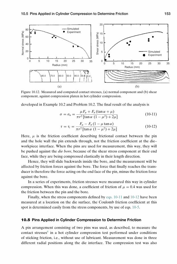
10.5 Pins Applied in Cylinder Compression to Determine Friction 153
80
60
40
20
00 5 10 15 20 25 30 35
0 5 10 15 20 25 30 35
Simulated Experiment
Simulated Experiment
Radius (mm)Radius (mm)
80.0 70.0 60.0 50.0 40.0 30.0 20.0
2 4 6 8 10 12 14 16
Nor
mal
str
ess
(MP
a)
She
ar s
tres
s (M
Pa)
20
15
10
5
0
(a) (b)
Figure 10.12. Measured and computed contact stresses, (a) normal component and (b) shearcomponent, against compression platen in hot cylinder compression.
developed in Example 10.2 and Problem 10.2. The final result of the analysis is
σ = σn = µFα + Fn (tan α + µ)πr2 [tan α (1 − µ2) + 2µ]
(10-11)
τ = τi = Fα − Fn (1 − µ tan α)πr2 [tan α (1 − µ2) + 2µ]
(10-12)
Here, µ is the friction coefficient describing frictional contact between the pinand the hole wall the pin extends through, not the friction coefficient at the die–workpiece interface. When the pins are used for measurement, this way, they willbe pushed against the die bore, because of the shear stress component at their endface, while they are being compressed elastically in their length direction.
Hence, they will slide backwards inside the bore, and the measurement will beaffected by friction forces against the bore. The force that finally reaches the trans-ducer is therefore the force acting on the end face of the pin, minus the friction forceagainst the bore.
In a series of experiments, friction stresses were measured this way in cylindercompression. When this was done, a coefficient of friction of µ = 0.4 was used forthe friction between the pin and the bore.
Finally, when the stress components defined by eqs. 10-11 and 10-12 have beenmeasured at a location on the die surface, the Coulomb friction coefficient at thisspot is determined easily from the stress components, by use of eqs. 10-5.
10.5 Pins Applied in Cylinder Compression to Determine Friction
A pin arrangement consisting of two pins was used, as described, to measure thecontact stresses8 in a hot cylinder compression test performed under conditionsof sticking friction, i.e., without use of lubricant. Measurement was done in threedifferent radial positions along the die interface. The compression test was also
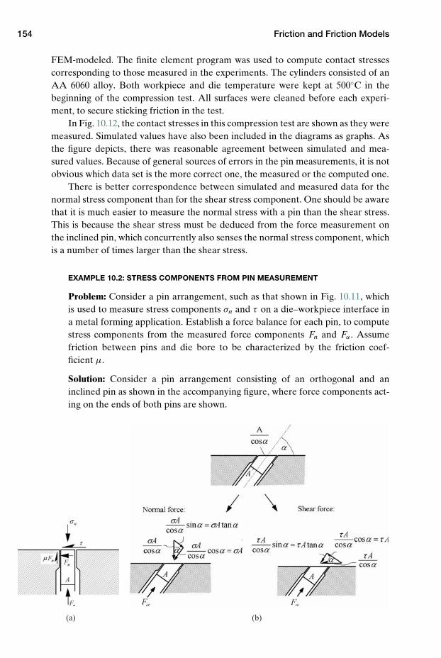
154 Friction and Friction Models
FEM-modeled. The finite element program was used to compute contact stressescorresponding to those measured in the experiments. The cylinders consisted of anAA 6060 alloy. Both workpiece and die temperature were kept at 500◦C in thebeginning of the compression test. All surfaces were cleaned before each experi-ment, to secure sticking friction in the test.
In Fig. 10.12, the contact stresses in this compression test are shown as they weremeasured. Simulated values have also been included in the diagrams as graphs. Asthe figure depicts, there was reasonable agreement between simulated and mea-sured values. Because of general sources of errors in the pin measurements, it is notobvious which data set is the more correct one, the measured or the computed one.
There is better correspondence between simulated and measured data for thenormal stress component than for the shear stress component. One should be awarethat it is much easier to measure the normal stress with a pin than the shear stress.This is because the shear stress must be deduced from the force measurement onthe inclined pin, which concurrently also senses the normal stress component, whichis a number of times larger than the shear stress.
EXAMPLE 10.2: STRESS COMPONENTS FROM PIN MEASUREMENT
Problem: Consider a pin arrangement, such as that shown in Fig. 10.11, whichis used to measure stress components σn and τ on a die–workpiece interface ina metal forming application. Establish a force balance for each pin, to computestress components from the measured force components Fn and Fα . Assumefriction between pins and die bore to be characterized by the friction coef-ficient µ.
Solution: Consider a pin arrangement consisting of an orthogonal and aninclined pin as shown in the accompanying figure, where force components act-ing on the ends of both pins are shown.
(a) (b)

Problems 155
With friction in the bore, there are friction forces counteracting the primaryforce components. For the orthogonally oriented pin, the normal and the fric-tion force against the bore can be expressed as follows (see the left-hand side ofthe figure):
FN = Aτ
Fµ = µFN = µAτ
The force equilibrium in the axial direction of the pin can then be expressedas
Fn = FN − Fµ = Aσn − µAτ = A (σn − µτ ) (10-13)
For the inclined pin, one correspondingly obtains the expressions
FN = σn A tan α − τ A = A (σn tan α − τ )
Fµ = µFN = µA (σn tan α − τ )
The force equilibrium in the axial direction of this pin then yields
Fα = FN − Fµ = A (σn tan α − τ ) − µA (σn tan α − τ )
= A [σn + τ tan α − µ (σn tan α − τ )] (10-14)
We have thus obtained two equations in which there are two unknownparameters, namely, σn and τ . From these equations, it is therefore straight-forward to solve for the stress components, when the forces Fn and Fα areknown from measurement. The result is that already given by eqs. 10-11 and10-12.
Problems
10.1 Friction is determined in ring compression testing. The following specimengeometry is used in the test: OD0 = 75 mm, ID0 = 37.5 mm, and h0 = 12.5 mm;see Fig. 10.9.
(a) Determine the ratio OD0 : ID0 : h0 for the ring specimen. Three metalswere tested in dry friction condition and in different lubricated conditions;see the accompanying table. In all cases, the final height of the specimenafter compression was h = 9 mm. The final inner ring diameter was mea-sured in each test, and results are given in the table.
(b) Determine the friction in each ring test, both as coefficient of friction andfriction factor. Use the graphs in Fig. 10.10 and the one accompanying thisproblem to determine the friction values.
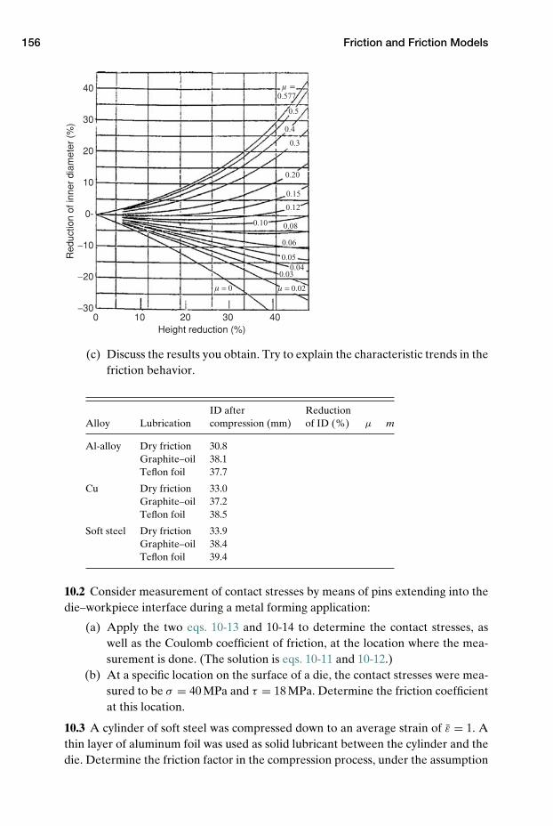
156 Friction and Friction Models
40
30
20
10
0-
−10
−20
−300 10 20 30 40
Height reduction (%)
Red
uctio
n of
inne
r di
amet
er (
%)
0.577
0.5
µ =
0.4
0.3
0.20
0.15
0.12
0.080.10
0.06
0.050.04
0.03
µ = 0.02µ = 0
(c) Discuss the results you obtain. Try to explain the characteristic trends in thefriction behavior.
ID after ReductionAlloy Lubrication compression (mm) of ID (%) µ m
Al-alloy Dry friction 30.8Graphite–oil 38.1Teflon foil 37.7
Cu Dry friction 33.0Graphite–oil 37.2Teflon foil 38.5
Soft steel Dry friction 33.9Graphite–oil 38.4Teflon foil 39.4
10.2 Consider measurement of contact stresses by means of pins extending into thedie–workpiece interface during a metal forming application:
(a) Apply the two eqs. 10-13 and 10-14 to determine the contact stresses, aswell as the Coulomb coefficient of friction, at the location where the mea-surement is done. (The solution is eqs. 10-11 and 10-12.)
(b) At a specific location on the surface of a die, the contact stresses were mea-sured to be σ = 40 MPa and τ = 18 MPa. Determine the friction coefficientat this location.
10.3 A cylinder of soft steel was compressed down to an average strain of ε = 1. Athin layer of aluminum foil was used as solid lubricant between the cylinder and thedie. Determine the friction factor in the compression process, under the assumption
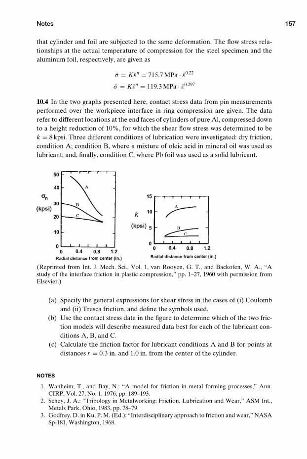
Notes 157
that cylinder and foil are subjected to the same deformation. The flow stress rela-tionships at the actual temperature of compression for the steel specimen and thealuminum foil, respectively, are given as
σ = Kεn = 715.7 MPa · ε0.22
σ = Kεn = 119.3 MPa · ε0.297
10.4 In the two graphs presented here, contact stress data from pin measurementsperformed over the workpiece interface in ring compression are given. The datarefer to different locations at the end faces of cylinders of pure Al, compressed downto a height reduction of 10%, for which the shear flow stress was determined to bek = 8 kpsi. Three different conditions of lubrication were investigated: dry friction,condition A; condition B, where a mixture of oleic acid in mineral oil was used aslubricant; and, finally, condition C, where Pb foil was used as a solid lubricant.
(Reprinted from Int. J. Mech. Sci., Vol. 1, van Rooyen, G. T., and Backofen, W. A., “Astudy of the interface friction in plastic compression,” pp. 1–27, 1960 with permission fromElsevier.)
(a) Specify the general expressions for shear stress in the cases of (i) Coulomband (ii) Tresca friction, and define the symbols used.
(b) Use the contact stress data in the figure to determine which of the two fric-tion models will describe measured data best for each of the lubricant con-ditions A, B, and C.
(c) Calculate the friction factor for lubricant conditions A and B for points atdistances r = 0.3 in. and 1.0 in. from the center of the cylinder.
NOTES
1. Wanheim, T., and Bay, N.: “A model for friction in metal forming processes,” Ann.CIRP, Vol. 27, No. 1, 1976, pp. 189–193.
2. Schey, J. A.: “Tribology in Metalworking: Friction, Lubrication and Wear,” ASM Int.,Metals Park, Ohio, 1983, pp. 78–79.
3. Godfrey, D. in Ku, P. M. (Ed.): “Interdisciplinary approach to friction and wear,” NASASp-181, Washington, 1968.

158 Friction and Friction Models
4. Suthcliffe, M. P. F., Lee, H. R., and Farrugia, D.: “Simulation of transfer layer formationin strip drawing of stainless steel,” Wear, Vol. 254, 2003, pp. 523–531.
5. Male, T., and Cockcroft, M. G.: “A method of the determination of the coefficient offriction of metals under conditions of bulk plastic deformation,” J. Inst. Metals, Vol. 93,1964–65, pp. 38–46.
6. Siebel, E., and Lueg, W.: Mitt. Kaiser Wilhelm Inst. Eisenforschung, Vol. 15, 1933, p. 1.7. van Rooyen, G. T., and Backofen, W. A.: “A study of the interface friction in plastic
compression,” Int. J. Mechanical Sciences, 1960, Vol. 1, pp. 1–27.8. Hansen, A. W., Welo, T., and Valberg, H.: “A technique for measuring stresses on the
tool surface,” Proc. 4th Int. Conf. on Technology of Plasticity, Beijing, China, 1993,Vol. 1, pp. 303–308.
REFERENCES
Bay, N.: “Modelling and testing of friction in forging,” in “New Developments in ForgingTechnology,” Mat-Info Werkstoff-Informationsgesellschaft, Frankfurt, 2007, pp. 233–252.
Lenard, J. G. (Ed.): “Metal Forming Science and Practice,” Elsevier, 2002.Mang, T.: “Die Schmierung in der Metallbearbeitung,” Vogel-Buchverlag, 1983.Schey, J. A.: “Tribology in Metalworking: Friction, Lubrication and Wear,” ASM Int., Metals
Park, Ohio, 1983.

11 Thermal Effects
The energy consumed in a metal forming operation, as, for instance, in a forgingstroke, is mainly transformed into heat, which leads to temperature rise in the dieand the workpiece. In heavy metal forming equipment, a lot of energy is supplied tothe workpiece this way, and there can be substantial global and local heating effectsin the workpiece material.
In many metal forming applications, there are limits on how high the tempera-ture of the workpiece can rise before one experiences problems such as reduced orunacceptable product quality. This is, for instance, the case in aluminum extrusion,where the maximum temperature of the metal near the outlet from the die shouldnot exceed a certain critical temperature. In this process, material defects, such assurface cracking due to hot tearing of the material, start to appear when this criticaltemperature is exceeded, and a usable profile can no longer be manufactured. Thisphenomenon is explained and discussed in this chapter.
In addition, it is shown how one can quantify different thermal effects in a metalforming process, such as heating due to plastic deformation inside the workpiece, andheating due to friction over its surface. When the workpiece has higher temperaturethan the dies, there is cooling against the dies, and the physics required to calculatethe cooling is shown for a simple two-dimensional case.
It is also explained how the temperature inside the tooling and on the surfaceof the workpiece can be measured by use of thermocouples. Use of pyrometry tomeasure the surface temperature on a body is also discussed. Finally, characteris-tic thermal conditions in some typical nonstationary and stationary metal formingprocesses are described by examples.
11.1 Thermal Effects in Metal Deformation Processes
When it comes to thermal effects, heat radiation is in many cases neglected in metalforming applications. But, for instance, hot forming of steels is performed at temper-atures as high as 1000–1200◦C. At these temperatures, loss of heat due to radiationbecomes significant and must be included if an accurate thermal analysis is to bedone. Al and Al alloys, however, are seldom formed at higher temperature than
159
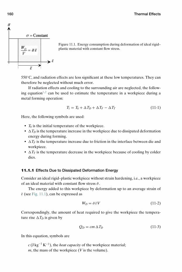
160 Thermal Effects
Figure 11.1. Energy consumption during deformation of ideal rigid–plastic material with constant flow stress.
550◦C, and radiation effects are less significant at these low temperatures. They cantherefore be neglected without much error.
If radiation effects and cooling to the surrounding air are neglected, the follow-ing equation1,2 can be used to estimate the temperature in a workpiece during ametal forming operation:
T1 = T0 + �TD + �TF − �TT (11-1)
Here, the following symbols are used:
� T0 is the initial temperature of the workpiece.� �TD is the temperature increase in the workpiece due to dissipated deformation
energy during forming.� �TF is the temperature increase due to friction in the interface between die and
workpiece.� �TT is the temperature decrease in the workpiece because of cooling by colder
dies.
11.1.1 Effects Due to Dissipated Deformation Energy
Consider an ideal rigid–plastic workpiece without strain hardening, i.e., a workpieceof an ideal material with constant flow stress σ .
The energy added to this workpiece by deformation up to an average strain ofε (see Fig. 11.1), can be expressed as
WD = σ εV (11-2)
Correspondingly, the amount of heat required to give the workpiece the tempera-ture rise �TD is given by
QD = cm �TD (11-3)
In this equation, symbols are
c (J kg−1 K−1), the heat capacity of the workpiece material;m, the mass of the workpiece (V is the volume).
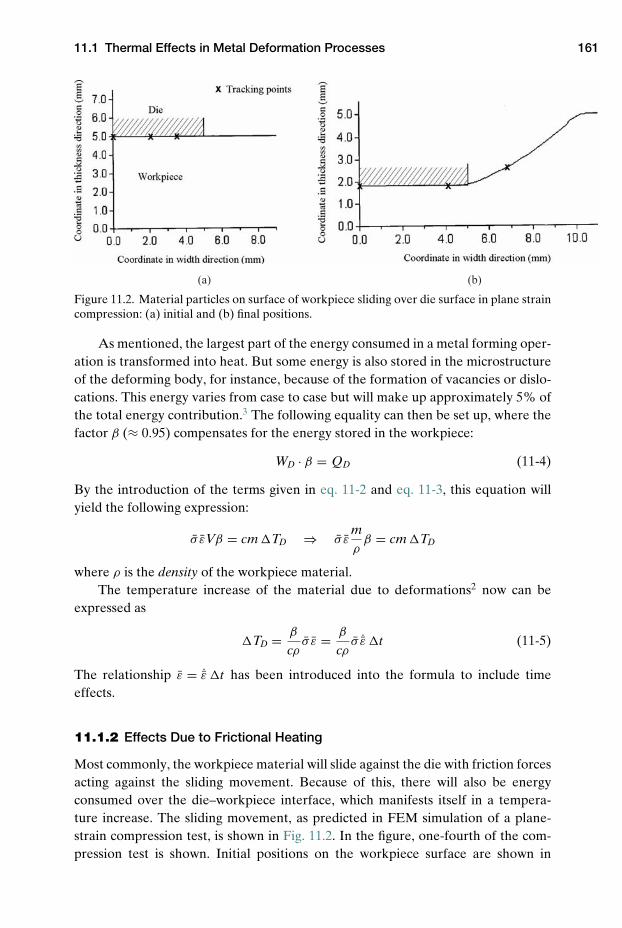
11.1 Thermal Effects in Metal Deformation Processes 161
(a) (b)
Figure 11.2. Material particles on surface of workpiece sliding over die surface in plane straincompression: (a) initial and (b) final positions.
As mentioned, the largest part of the energy consumed in a metal forming oper-ation is transformed into heat. But some energy is also stored in the microstructureof the deforming body, for instance, because of the formation of vacancies or dislo-cations. This energy varies from case to case but will make up approximately 5% ofthe total energy contribution.3 The following equality can then be set up, where thefactor β (≈ 0.95) compensates for the energy stored in the workpiece:
WD · β = QD (11-4)
By the introduction of the terms given in eq. 11-2 and eq. 11-3, this equation willyield the following expression:
σ εVβ = cm �TD ⇒ σ εmρ
β = cm �TD
where ρ is the density of the workpiece material.The temperature increase of the material due to deformations2 now can be
expressed as
�TD = β
cρσ ε = β
cρσ ˙ε �t (11-5)
The relationship ε = ˙ε �t has been introduced into the formula to include timeeffects.
11.1.2 Effects Due to Frictional Heating
Most commonly, the workpiece material will slide against the die with friction forcesacting against the sliding movement. Because of this, there will also be energyconsumed over the die–workpiece interface, which manifests itself in a tempera-ture increase. The sliding movement, as predicted in FEM simulation of a plane-strain compression test, is shown in Fig. 11.2. In the figure, one-fourth of the com-pression test is shown. Initial positions on the workpiece surface are shown in
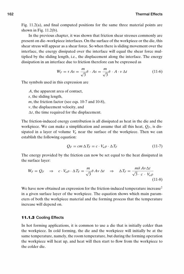
162 Thermal Effects
Fig. 11.2(a), and final computed positions for the same three material points areshown in Fig. 11.2(b).
In the previous chapter, it was shown that friction shear stresses commonly arepresent on die–workpiece interfaces. On the surface of the workpiece or the die, thisshear stress will appear as a shear force. So when there is sliding movement over theinterface, the energy dissipated over the interface will equal the shear force mul-tiplied by the sliding length, i.e., the displacement along the interface. The energydissipation in an interface due to friction therefore can be expressed as
WF = τ As = m√3σ · As = m√
3σ · A · v �t (11-6)
The symbols used in this expression are
A, the apparent area of contact,s, the sliding length,m, the friction factor (see eqs. 10-7 and 10-8),v, the displacement velocity, and�t , the time required for the displacement.
The friction-induced energy contribution is all dissipated as heat in the die and theworkpiece. We can make a simplification and assume that all this heat, QF , is dis-sipated in a layer of volume Va near the surface of the workpiece. Then we canestablish the following equation:
QF = cm �TF = c · Vaρ · �TF (11-7)
The energy provided by the friction can now be set equal to the heat dissipated inthe surface layer:
WF = QF ⇒ c · Vaρ · �TF = m√3σ Av �t ⇒ �TF = mσ Av�t√
3 · c · Vaρ
(11-8)
We have now obtained an expression for the friction-induced temperature increase2
in a given surface layer of the workpiece. The equation shows which main param-eters of both the workpiece material and the forming process that the temperatureincrease will depend on.
11.1.3 Cooling Effects
In hot forming applications, it is common to use a die that is initially colder thanthe workpiece. In cold forming, the die and the workpiece will initially be at thesame temperature, namely, the room temperature, but during the forming operationthe workpiece will heat up, and heat will then start to flow from the workpiece tothe colder die.
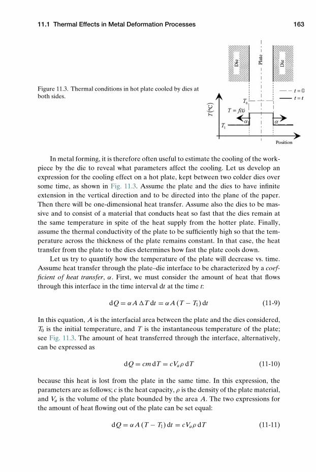
11.1 Thermal Effects in Metal Deformation Processes 163
Figure 11.3. Thermal conditions in hot plate cooled by dies atboth sides.
In metal forming, it is therefore often useful to estimate the cooling of the work-piece by the die to reveal what parameters affect the cooling. Let us develop anexpression for the cooling effect on a hot plate, kept between two colder dies oversome time, as shown in Fig. 11.3. Assume the plate and the dies to have infiniteextension in the vertical direction and to be directed into the plane of the paper.Then there will be one-dimensional heat transfer. Assume also the dies to be mas-sive and to consist of a material that conducts heat so fast that the dies remain atthe same temperature in spite of the heat supply from the hotter plate. Finally,assume the thermal conductivity of the plate to be sufficiently high so that the tem-perature across the thickness of the plate remains constant. In that case, the heattransfer from the plate to the dies determines how fast the plate cools down.
Let us try to quantify how the temperature of the plate will decrease vs. time.Assume heat transfer through the plate–die interface to be characterized by a coef-ficient of heat transfer, α. First, we must consider the amount of heat that flowsthrough this interface in the time interval dt at the time t:
dQ = αA �T dt = αA (T − T1) dt (11-9)
In this equation, A is the interfacial area between the plate and the dies considered,T0 is the initial temperature, and T is the instantaneous temperature of the plate;see Fig. 11.3. The amount of heat transferred through the interface, alternatively,can be expressed as
dQ = cm dT = cVaρ dT (11-10)
because this heat is lost from the plate in the same time. In this expression, theparameters are as follows; c is the heat capacity, ρ is the density of the plate material,and Va is the volume of the plate bounded by the area A. The two expressions forthe amount of heat flowing out of the plate can be set equal:
dQ = αA (T − T1) dt = cVaρ dT (11-11)
164 Thermal Effects
This expression can be reorganized and integrated:∫ t
0
αAcρVa
dt =∫ T0
T
dTT − T1
⇒ αAcρVa
t = [ln(T − T1)]T0T
= ln (T0 − T1) − ln (T − T1) = lnT0 − T1
T − T1
[Formula of integration:∫
dx/(ax + b) = (1/a) ln (ax + b), where a and b areconstants and x �= 0]. Further development of the expression yields2
T − T1
T0 − T1= exp
(− αA
cρVat)
⇒ T = T1 + (T0 − T1) exp(
− αtcρ
AVa
)
The ratio Va/A = h represents the thickness of the plate and can be added into theexpression to give
T = f (t) = T1 + (T0 − T1) exp(
− αtcρh
)(11-12)
We have now determined the temperature of the plate as function of time. Aseq. 11-12 shows, the temperature is predicted to decrease exponentially with time,from the initial temperature T0 to the die temperature T1. This means that the tem-perature of the plate will drop as a transient down to the die temperature. How rapidthe temperature drop is, and how it is influenced by various process parameters, isalso revealed by the equation.
In the beginning of the chapter, the current temperature in a workpiece sub-jected to metal forming was denoted by T1; see eq. 11-1. This equation now can bereformulated as follows:
T1 = T0 + �TD + �TF − �TT = (T0 − �TT) + �TD + �TF
= T + �TD + �TF (11-13)
Here, the term T includes the cooling effect because of the use of colder dies.
11.2 Temperature Measurement
In metal forming applications, two different techniques, namely, thermocouple andpyrometer measurement, are commonly used to determine either the die or theworkpiece temperature.
Steel has an approximately constant emissivity at a fixed temperature, i.e., acertain fraction of its heat is lost per time unit, due to heat radiation at this temper-ature. Because of this, the surface temperature of visible surfaces of a workpiece ofsteel can be measured with good accuracy using radiation pyrometry. A pyrometeris an optical device that receives radiated energy from a small area on the surface ofa body and that, from the amount of received energy, computes the mean surfacetemperature of the area. The temperature of invisible surfaces of a workpiece, suchas those inside a die, can of course not be determined by pyrometry.
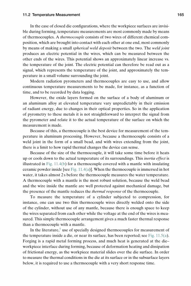
11.2 Temperature Measurement 165
In the case of closed die configurations, where the workpiece surfaces are invisi-ble during forming, temperature measurements are most commonly made by meansof thermocouples. A thermocouple consists of two wires of different chemical com-position, which are brought into contact with each other at one end, most commonlyby means of making a small spherical weld deposit between the two. The weld jointproduces an electric potential in the wires, which can be measured between theother ends of the wires. This potential shows an approximately linear increase vs.the temperature of the joint. The electric potential can therefore be read out as asignal, which represents the temperature of the joint, and approximately the tem-perature in a small volume surrounding the joint.
Modern radiation pyrometers and thermocouples are easy to use, and allowcontinuous temperature measurements to be made, for instance, as a function oftime, and to be recorded by data logging.
However, the oxide layers formed on the surface of a body of aluminum oran aluminum alloy at elevated temperature vary unpredictably in their emissionof radiant energy, due to changes in their optical properties. So in the applicationof pyrometry to these metals it is not straightforward to interpret the signal fromthe pyrometer and relate it to the actual temperature of the surface on which themeasurement is made.
Because of this, a thermocouple is the best device for measurement of the tem-perature in aluminum processing. However, because a thermocouple consists of aweld joint in the form of a small bead, and with wires extending from the joint,there is a limit to how rapid thermal changes the device can sense.
Because of the size of the thermocouple, it will take some time before it heatsup or cools down to the actual temperature of its surroundings. This inertia effect isillustrated in Fig. 11.4(b) for a thermocouple covered with a mantle with insulatingceramic powder inside [see Fig. 11.4(a)]. When the thermocouple is immersed in hotwater, it takes almost 2 s before the thermocouple measures the water temperature.A thermocouple with a mantle is the most robust solution, because the weld beadand the wire inside the mantle are well protected against mechanical damage, butthe presence of the mantle reduces the thermal response of the thermocouple.
To measure the temperature of a cylinder subjected to compression, forinstance, one can use two thin thermocouple wires directly welded onto the sideof the cylinder, without use of any mantle, because there is enough space to keepthe wires separated from each other while the voltage at the end of the wires is mea-sured. This simple thermocouple arrangement gives a much faster thermal responsethan a thermocouple with a mantle.
In the literature,5 use of specially designed thermocouples for measurement ofthe temperature inside a die, or near its surface, has been reported; see Fig. 11.5(a).Forging is a rapid metal forming process, and much heat is generated at the die–workpiece interface during forming, because of deformation heating and dissipationof frictional energy, as the workpiece material slides over the die surface. In orderto measure the thermal conditions in the die at its surface or in the subsurface layersbelow, it is required to use a thermocouple with a very short response time.
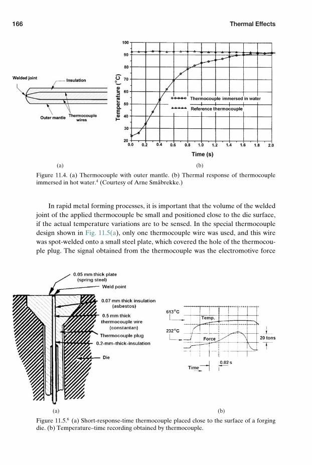
166 Thermal Effects
(a) (b)
Figure 11.4. (a) Thermocouple with outer mantle. (b) Thermal response of thermocoupleimmersed in hot water.4 (Courtesy of Arne Smabrekke.)
In rapid metal forming processes, it is important that the volume of the weldedjoint of the applied thermocouple be small and positioned close to the die surface,if the actual temperature variations are to be sensed. In the special thermocoupledesign shown in Fig. 11.5(a), only one thermocouple wire was used, and this wirewas spot-welded onto a small steel plate, which covered the hole of the thermocou-ple plug. The signal obtained from the thermocouple was the electromotive force
(a) (b)
Figure 11.5.6 (a) Short-response-time thermocouple placed close to the surface of a forgingdie. (b) Temperature–time recording obtained by thermocouple.
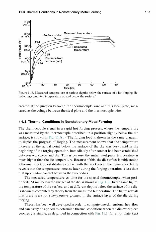
11.3 Thermal Conditions in Nonstationary Metal Forming 167
Figure 11.6. Measured temperature at various depths below the surface of a hot-forging die,including computed temperature on and below the surface.6
created at the junction between the thermocouple wire and this steel plate, mea-sured as the voltage between the steel plate and the thermocouple wire.
11.3 Thermal Conditions in Nonstationary Metal Forming
The thermocouple signal in a rapid hot forging process, where the temperaturewas measured by the thermocouple described, in a position slightly below the diesurface, is shown in Fig. 11.5(b). The forging load is shown in the same diagram,to depict the progress of forging. The measurement shows that the temperatureincrease at the actual point below the surface of the die was very rapid in thebeginning of the forging operation, immediately after contact had been establishedbetween workpiece and die. This is because the initial workpiece temperature ismuch higher than the die temperature. Because of this, the die surface is subjected toa thermal shock on establishing contact with the workpiece. The figure also clearlyreveals that the temperature increase later during the forging operation is less thanthat upon initial contact between the two bodies.
The measured temperature vs. time for the special thermocouple, when posi-tioned 0.51 mm below the surface of the die, is shown in Fig. 11.6. In the same figure,the temperature of the surface, and at different depths below the surface of the die,is shown as computed by theory from the measured temperature. The figure revealsthat there is a strong temperature gradient in the surface layer of the die duringforging.
Theory has been well developed in order to compute one-dimensional heat flowand can easily be applied to determine thermal conditions when the die–workpiecegeometry is simple, as described in connection with Fig. 11.3, for a hot plate kept
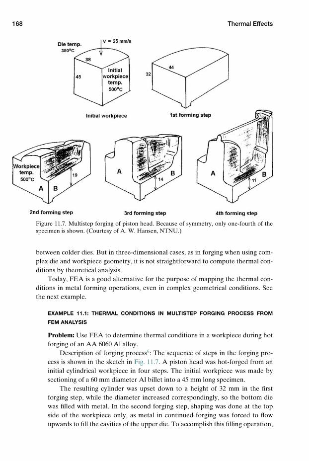
168 Thermal Effects
Figure 11.7. Multistep forging of piston head. Because of symmetry, only one-fourth of thespecimen is shown. (Courtesy of A. W. Hansen, NTNU.)
between colder dies. But in three-dimensional cases, as in forging when using com-plex die and workpiece geometry, it is not straightforward to compute thermal con-ditions by theoretical analysis.
Today, FEA is a good alternative for the purpose of mapping the thermal con-ditions in metal forming operations, even in complex geometrical conditions. Seethe next example.
EXAMPLE 11.1: THERMAL CONDITIONS IN MULTISTEP FORGING PROCESS FROM
FEM ANALYSIS
Problem: Use FEA to determine thermal conditions in a workpiece during hotforging of an AA 6060 Al alloy.
Description of forging process6: The sequence of steps in the forging pro-cess is shown in the sketch in Fig. 11.7. A piston head was hot-forged from aninitial cylindrical workpiece in four steps. The initial workpiece was made bysectioning of a 60 mm diameter Al billet into a 45 mm long specimen.
The resulting cylinder was upset down to a height of 32 mm in the firstforging step, while the diameter increased correspondingly, so the bottom diewas filled with metal. In the second forging step, shaping was done at the topside of the workpiece only, as metal in continued forging was forced to flowupwards to fill the cavities of the upper die. To accomplish this filling operation,
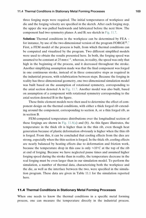
11.4 Thermal Conditions in Stationary Metal Forming Processes 169
three forging steps were required. The initial temperatures of workpiece anddie and the forging velocity are specified in the sketch. After each forging step,the upper die was pulled backwards and lubricated before the next blow. Thecomponent had two symmetry planes A and B; see sketch in Fig. 11.7.
Solution: Thermal conditions in the workpiece can be determined by FEA –for instance, by use of the two-dimensional version of the program FORGE R©.7
First, a FEM model of the process is built, from which thermal conditions canbe computed and visualized by the program. Two different simplified modelswere used to obtain the results presented here. In both, the forging speed wasassumed to be constant at 25 mm s−1, whereas, in reality, the speed was only thathigh in the beginning of the process, and it decreased throughout the stroke.Another simplifying assumption made was that the final component was forgedin one continuous stroke, instead of in three consecutive steps as required inthe industrial process, with relubrication between steps. Because the forging inreality has three-dimensional geometry, one two-dimensional simulation modelwas built based on the assumption of rotational symmetry, corresponding tothe axial section denoted A in Fig. 11.7. Another model was also built, basedon assumption of a component with rotational symmetry corresponding to theaxial section denoted B in the figure.
These finite element models were then used to determine the effect of com-ponent design on the thermal conditions, with either a thick forged rib extend-ing around the component, corresponding to section A, or a thin forged rib, asin section B.
FEM-computed temperature distributions over the longitudinal section ofthese forgings are shown in Fig. 11.8(a) and (b). As this figure illustrates, thetemperature in the thick rib is higher than in the thin rib, even though heatgeneration because of plastic deformation obviously is higher when the thin ribis forged. From this, it can be concluded that cooling effects from the dies arestrong, especially when the thin section is forged. In the thick rib, cooling effectsare nearly balanced by heating effects due to deformation and friction work,because the temperature drop in this case is only ≈10◦C at the top of the ribat end of forging. Because we have neglected pause times and assumed higherforging speed during the stroke than in reality, the temperature decrease in thereal forging must be even larger than in our simulation model. To perform thesimulation, a number of thermal data, characterizing both the workpiece andthe die, as well as the interface between the two, were specified in the simula-tion program. These data are given in Table 11.1 for the simulation reportedhere.
11.4 Thermal Conditions in Stationary Metal Forming Processes
When one needs to know the thermal conditions in a specific metal formingprocess, one can measure the temperature directly in the industrial process.
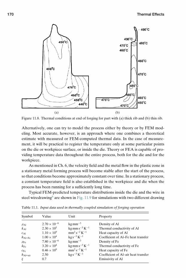
170 Thermal Effects
(a) (b)
Figure 11.8. Thermal conditions at end of forging for part with (a) thick rib and (b) thin rib.
Alternatively, one can try to model the process either by theory or by FEM mod-eling. Most accurate, however, is an approach where one combines a theoreticalestimate with measured or FEM-computed thermal data. In the case of measure-ment, it will be practical to register the temperature only at some particular pointson the die or workpiece surface, or inside the die. Theory or FEA is capable of pro-viding temperature data throughout the entire process, both for the die and for theworkpiece.
As mentioned in Ch. 6, the velocity field and the metal flow in the plastic zone ina stationary metal forming process will become stable after the start of the process,so that conditions become approximately constant over time. In a stationary process,a constant temperature field is also established in the workpiece and die when theprocess has been running for a sufficiently long time.
Typical FEM-predicted temperature distributions inside the die and the wire insteel wiredrawing8 are shown in Fig. 11.9 for simulations with two different drawing
Table 11.1. Input data used in thermally coupled simulation of forging operation
Symbol Value Unit Property
ρAl 2.70 × 10⁻⁶ kg mm−3 Density of AlkAl 2.30 × 10⁵ kg mm s−3 K−1 Thermal conductivity of AlcAl 1.10 × 109 mm2 s−2 K−1 Heat capacity of AlhAl–Fe 1.00 × 10⁴ kg s−3 K−1 Coefficient of Al–Fe heat transferρFe 7.80 × 10⁻⁶ kg mm−3 Density of FekFe 3.20 × 10⁴ kg mm s−3 K−1 Thermal conductivity of FecFe 0.46 × 109 mm2 s−2 K−1 Heat capacity of FehAl–air 2.50 kg s−3 K−1 Coefficient of Al–air heat transferξ 0.7 Emissivity of Al
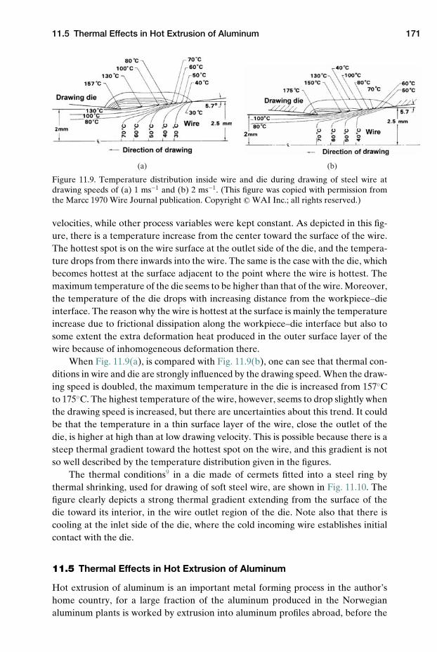
11.5 Thermal Effects in Hot Extrusion of Aluminum 171
(a) (b)
Figure 11.9. Temperature distribution inside wire and die during drawing of steel wire atdrawing speeds of (a) 1 ms−1 and (b) 2 ms−1. (This figure was copied with permission fromthe Marcc 1970 Wire Journal publication. Copyright c© WAI Inc.; all rights reserved.)
velocities, while other process variables were kept constant. As depicted in this fig-ure, there is a temperature increase from the center toward the surface of the wire.The hottest spot is on the wire surface at the outlet side of the die, and the tempera-ture drops from there inwards into the wire. The same is the case with the die, whichbecomes hottest at the surface adjacent to the point where the wire is hottest. Themaximum temperature of the die seems to be higher than that of the wire. Moreover,the temperature of the die drops with increasing distance from the workpiece–dieinterface. The reason why the wire is hottest at the surface is mainly the temperatureincrease due to frictional dissipation along the workpiece–die interface but also tosome extent the extra deformation heat produced in the outer surface layer of thewire because of inhomogeneous deformation there.
When Fig. 11.9(a), is compared with Fig. 11.9(b), one can see that thermal con-ditions in wire and die are strongly influenced by the drawing speed. When the draw-ing speed is doubled, the maximum temperature in the die is increased from 157◦Cto 175◦C. The highest temperature of the wire, however, seems to drop slightly whenthe drawing speed is increased, but there are uncertainties about this trend. It couldbe that the temperature in a thin surface layer of the wire, close the outlet of thedie, is higher at high than at low drawing velocity. This is possible because there is asteep thermal gradient toward the hottest spot on the wire, and this gradient is notso well described by the temperature distribution given in the figures.
The thermal conditions9 in a die made of cermets fitted into a steel ring bythermal shrinking, used for drawing of soft steel wire, are shown in Fig. 11.10. Thefigure clearly depicts a strong thermal gradient extending from the surface of thedie toward its interior, in the wire outlet region of the die. Note also that there iscooling at the inlet side of the die, where the cold incoming wire establishes initialcontact with the die.
11.5 Thermal Effects in Hot Extrusion of Aluminum
Hot extrusion of aluminum is an important metal forming process in the author’shome country, for a large fraction of the aluminum produced in the Norwegianaluminum plants is worked by extrusion into aluminum profiles abroad, before the
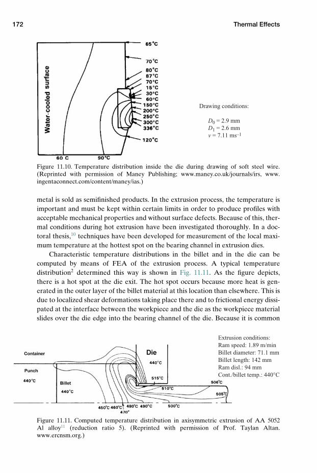
172 Thermal Effects
Drawing conditions:
D0 = 2.9 mm D1 = 2.6 mm v = 7.11 ms–1
Figure 11.10. Temperature distribution inside the die during drawing of soft steel wire.(Reprinted with permission of Maney Publishing; www.maney.co.uk/journals/irs, www.ingentaconnect.com/content/maney/ias.)
metal is sold as semifinished products. In the extrusion process, the temperature isimportant and must be kept within certain limits in order to produce profiles withacceptable mechanical properties and without surface defects. Because of this, ther-mal conditions during hot extrusion have been investigated thoroughly. In a doc-toral thesis,10 techniques have been developed for measurement of the local maxi-mum temperature at the hottest spot on the bearing channel in extrusion dies.
Characteristic temperature distributions in the billet and in the die can becomputed by means of FEA of the extrusion process. A typical temperaturedistribution2 determined this way is shown in Fig. 11.11. As the figure depicts,there is a hot spot at the die exit. The hot spot occurs because more heat is gen-erated in the outer layer of the billet material at this location than elsewhere. This isdue to localized shear deformations taking place there and to frictional energy dissi-pated at the interface between the workpiece and the die as the workpiece materialslides over the die edge into the bearing channel of the die. Because it is common
Extrusion conditions:Ram speed: 1.89 m/min Billet diameter: 71.1 mmBillet length: 142 mm Ram disl.: 94 mm Cont./billet temp.: 440°C
Figure 11.11. Computed temperature distribution in axisymmetric extrusion of AA 5052Al alloy11 (reduction ratio 5). (Reprinted with permission of Prof. Taylan Altan.www.ercnsm.org.)
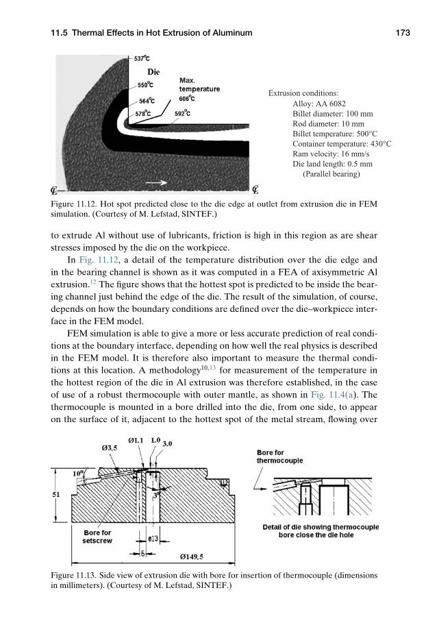
11.5 Thermal Effects in Hot Extrusion of Aluminum 173
Extrusion conditions:Alloy: AA 6082 Billet diameter: 100 mm Rod diameter: 10 mm Billet temperature: 500°C Container temperature: 430°CRam velocity: 16 mm/s Die land length: 0.5 mm (Parallel bearing)
Figure 11.12. Hot spot predicted close to the die edge at outlet from extrusion die in FEMsimulation. (Courtesy of M. Lefstad, SINTEF.)
to extrude Al without use of lubricants, friction is high in this region as are shearstresses imposed by the die on the workpiece.
In Fig. 11.12, a detail of the temperature distribution over the die edge andin the bearing channel is shown as it was computed in a FEA of axisymmetric Alextrusion.12 The figure shows that the hottest spot is predicted to be inside the bear-ing channel just behind the edge of the die. The result of the simulation, of course,depends on how the boundary conditions are defined over the die–workpiece inter-face in the FEM model.
FEM simulation is able to give a more or less accurate prediction of real condi-tions at the boundary interface, depending on how well the real physics is describedin the FEM model. It is therefore also important to measure the thermal condi-tions at this location. A methodology10,13 for measurement of the temperature inthe hottest region of the die in Al extrusion was therefore established, in the caseof use of a robust thermocouple with outer mantle, as shown in Fig. 11.4(a). Thethermocouple is mounted in a bore drilled into the die, from one side, to appearon the surface of it, adjacent to the hottest spot of the metal stream, flowing over
Figure 11.13. Side view of extrusion die with bore for insertion of thermocouple (dimensionsin millimeters). (Courtesy of M. Lefstad, SINTEF.)
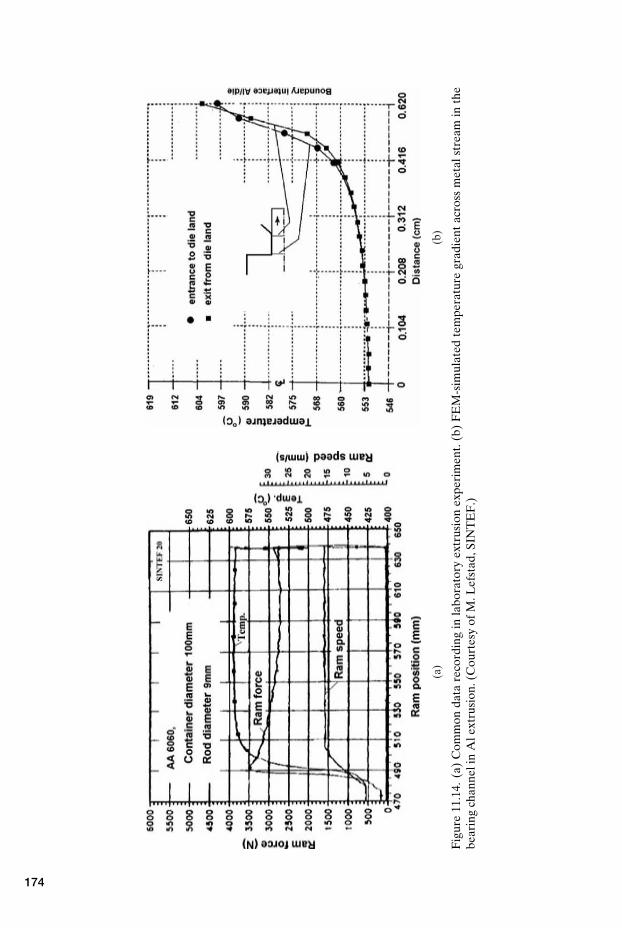
(a)
(b)
Fig
ure
11.1
4.(a
)C
omm
onda
tare
cord
ing
inla
bora
tory
extr
usio
nex
peri
men
t.(b
)F
EM
-sim
ulat
edte
mpe
ratu
regr
adie
ntac
ross
met
alst
ream
inth
ebe
arin
gch
anne
lin
Ale
xtru
sion
.(C
ourt
esy
ofM
.Lef
stad
,SIN
TE
F.)
174
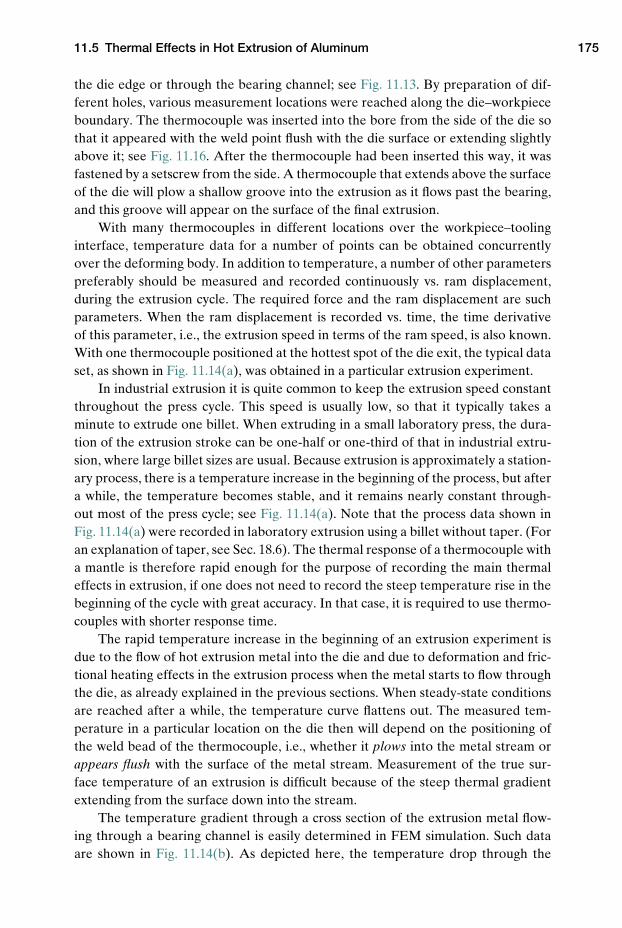
11.5 Thermal Effects in Hot Extrusion of Aluminum 175
the die edge or through the bearing channel; see Fig. 11.13. By preparation of dif-ferent holes, various measurement locations were reached along the die–workpieceboundary. The thermocouple was inserted into the bore from the side of the die sothat it appeared with the weld point flush with the die surface or extending slightlyabove it; see Fig. 11.16. After the thermocouple had been inserted this way, it wasfastened by a setscrew from the side. A thermocouple that extends above the surfaceof the die will plow a shallow groove into the extrusion as it flows past the bearing,and this groove will appear on the surface of the final extrusion.
With many thermocouples in different locations over the workpiece–toolinginterface, temperature data for a number of points can be obtained concurrentlyover the deforming body. In addition to temperature, a number of other parameterspreferably should be measured and recorded continuously vs. ram displacement,during the extrusion cycle. The required force and the ram displacement are suchparameters. When the ram displacement is recorded vs. time, the time derivativeof this parameter, i.e., the extrusion speed in terms of the ram speed, is also known.With one thermocouple positioned at the hottest spot of the die exit, the typical dataset, as shown in Fig. 11.14(a), was obtained in a particular extrusion experiment.
In industrial extrusion it is quite common to keep the extrusion speed constantthroughout the press cycle. This speed is usually low, so that it typically takes aminute to extrude one billet. When extruding in a small laboratory press, the dura-tion of the extrusion stroke can be one-half or one-third of that in industrial extru-sion, where large billet sizes are usual. Because extrusion is approximately a station-ary process, there is a temperature increase in the beginning of the process, but aftera while, the temperature becomes stable, and it remains nearly constant through-out most of the press cycle; see Fig. 11.14(a). Note that the process data shown inFig. 11.14(a) were recorded in laboratory extrusion using a billet without taper. (Foran explanation of taper, see Sec. 18.6). The thermal response of a thermocouple witha mantle is therefore rapid enough for the purpose of recording the main thermaleffects in extrusion, if one does not need to record the steep temperature rise in thebeginning of the cycle with great accuracy. In that case, it is required to use thermo-couples with shorter response time.
The rapid temperature increase in the beginning of an extrusion experiment isdue to the flow of hot extrusion metal into the die and due to deformation and fric-tional heating effects in the extrusion process when the metal starts to flow throughthe die, as already explained in the previous sections. When steady-state conditionsare reached after a while, the temperature curve flattens out. The measured tem-perature in a particular location on the die then will depend on the positioning ofthe weld bead of the thermocouple, i.e., whether it plows into the metal stream orappears flush with the surface of the metal stream. Measurement of the true sur-face temperature of an extrusion is difficult because of the steep thermal gradientextending from the surface down into the stream.
The temperature gradient through a cross section of the extrusion metal flow-ing through a bearing channel is easily determined in FEM simulation. Such dataare shown in Fig. 11.14(b). As depicted here, the temperature drop through the
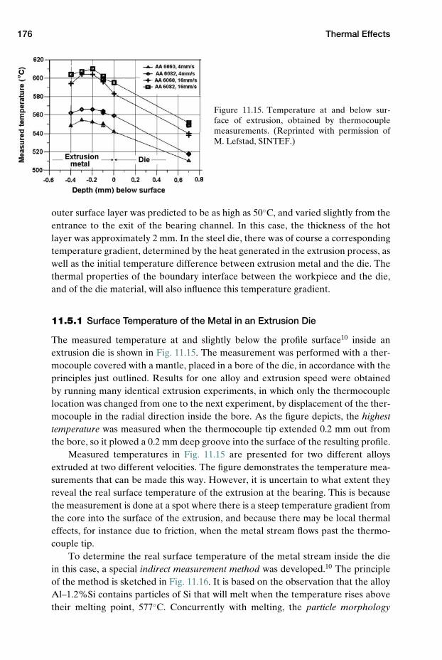
176 Thermal Effects
Figure 11.15. Temperature at and below sur-face of extrusion, obtained by thermocouplemeasurements. (Reprinted with permission ofM. Lefstad, SINTEF.)
outer surface layer was predicted to be as high as 50◦C, and varied slightly from theentrance to the exit of the bearing channel. In this case, the thickness of the hotlayer was approximately 2 mm. In the steel die, there was of course a correspondingtemperature gradient, determined by the heat generated in the extrusion process, aswell as the initial temperature difference between extrusion metal and the die. Thethermal properties of the boundary interface between the workpiece and the die,and of the die material, will also influence this temperature gradient.
11.5.1 Surface Temperature of the Metal in an Extrusion Die
The measured temperature at and slightly below the profile surface10 inside anextrusion die is shown in Fig. 11.15. The measurement was performed with a ther-mocouple covered with a mantle, placed in a bore of the die, in accordance with theprinciples just outlined. Results for one alloy and extrusion speed were obtainedby running many identical extrusion experiments, in which only the thermocouplelocation was changed from one to the next experiment, by displacement of the ther-mocouple in the radial direction inside the bore. As the figure depicts, the highesttemperature was measured when the thermocouple tip extended 0.2 mm out fromthe bore, so it plowed a 0.2 mm deep groove into the surface of the resulting profile.
Measured temperatures in Fig. 11.15 are presented for two different alloysextruded at two different velocities. The figure demonstrates the temperature mea-surements that can be made this way. However, it is uncertain to what extent theyreveal the real surface temperature of the extrusion at the bearing. This is becausethe measurement is done at a spot where there is a steep temperature gradient fromthe core into the surface of the extrusion, and because there may be local thermaleffects, for instance due to friction, when the metal stream flows past the thermo-couple tip.
To determine the real surface temperature of the metal stream inside the diein this case, a special indirect measurement method was developed.10 The principleof the method is sketched in Fig. 11.16. It is based on the observation that the alloyAl–1.2%Si contains particles of Si that will melt when the temperature rises abovetheir melting point, 577◦C. Concurrently with melting, the particle morphology
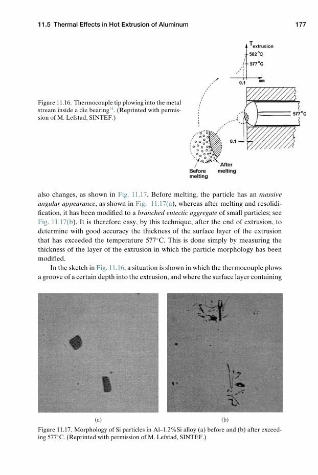
11.5 Thermal Effects in Hot Extrusion of Aluminum 177
Figure 11.16. Thermocouple tip plowing into the metalstream inside a die bearing14. (Reprinted with permis-sion of M. Lefstad, SINTEF.)
also changes, as shown in Fig. 11.17. Before melting, the particle has an massiveangular appearance, as shown in Fig. 11.17(a), whereas after melting and resolidi-fication, it has been modified to a branched eutectic aggregate of small particles; seeFig. 11.17(b). It is therefore easy, by this technique, after the end of extrusion, todetermine with good accuracy the thickness of the surface layer of the extrusionthat has exceeded the temperature 577◦C. This is done simply by measuring thethickness of the layer of the extrusion in which the particle morphology has beenmodified.
In the sketch in Fig. 11.16, a situation is shown in which the thermocouple plowsa groove of a certain depth into the extrusion, and where the surface layer containing
(a) (b)
Figure 11.17. Morphology of Si particles in Al–1.2%Si alloy (a) before and (b) after exceed-ing 577◦C. (Reprinted with permission of M. Lefstad, SINTEF.)
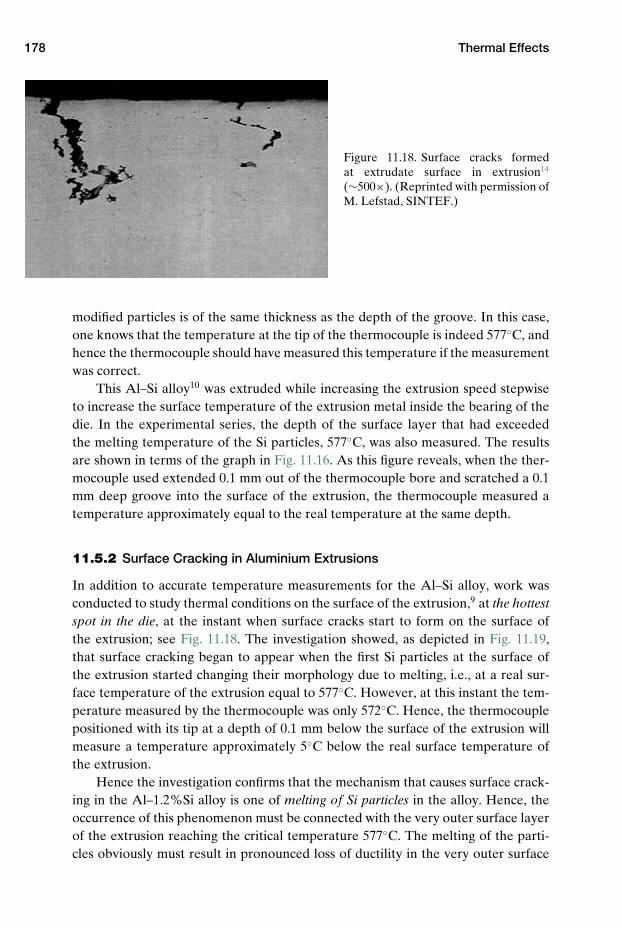
178 Thermal Effects
Figure 11.18. Surface cracks formedat extrudate surface in extrusion14
(∼500×). (Reprinted with permission ofM. Lefstad, SINTEF.)
modified particles is of the same thickness as the depth of the groove. In this case,one knows that the temperature at the tip of the thermocouple is indeed 577◦C, andhence the thermocouple should have measured this temperature if the measurementwas correct.
This Al–Si alloy10 was extruded while increasing the extrusion speed stepwiseto increase the surface temperature of the extrusion metal inside the bearing of thedie. In the experimental series, the depth of the surface layer that had exceededthe melting temperature of the Si particles, 577◦C, was also measured. The resultsare shown in terms of the graph in Fig. 11.16. As this figure reveals, when the ther-mocouple used extended 0.1 mm out of the thermocouple bore and scratched a 0.1mm deep groove into the surface of the extrusion, the thermocouple measured atemperature approximately equal to the real temperature at the same depth.
11.5.2 Surface Cracking in Aluminium Extrusions
In addition to accurate temperature measurements for the Al–Si alloy, work wasconducted to study thermal conditions on the surface of the extrusion,9 at the hottestspot in the die, at the instant when surface cracks start to form on the surface ofthe extrusion; see Fig. 11.18. The investigation showed, as depicted in Fig. 11.19,that surface cracking began to appear when the first Si particles at the surface ofthe extrusion started changing their morphology due to melting, i.e., at a real sur-face temperature of the extrusion equal to 577◦C. However, at this instant the tem-perature measured by the thermocouple was only 572◦C. Hence, the thermocouplepositioned with its tip at a depth of 0.1 mm below the surface of the extrusion willmeasure a temperature approximately 5◦C below the real surface temperature ofthe extrusion.
Hence the investigation confirms that the mechanism that causes surface crack-ing in the Al–1.2%Si alloy is one of melting of Si particles in the alloy. Hence, theoccurrence of this phenomenon must be connected with the very outer surface layerof the extrusion reaching the critical temperature 577◦C. The melting of the parti-cles obviously must result in pronounced loss of ductility in the very outer surface
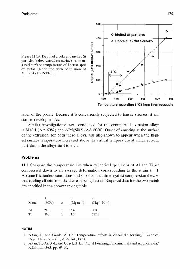
Problems 179
Figure 11.19. Depth of cracks and melted Siparticles below extrudate surface vs. mea-sured surface temperature of hottest spotof metal. (Reprinted with permission ofM. Lefstad, SINTEF.)
layer of the profile. Because it is concurrently subjected to tensile stresses, it willstart to develop cracks.
Similar investigations9 were conducted for the commercial extrusion alloysAlMgSi1 (AA 6082) and AlMgSi0.5 (AA 6060). Onset of cracking at the surfaceof the extrusion, for both these alloys, was also shown to appear when the high-est surface temperature increased above the critical temperature at which eutecticparticles in the alloys start to melt.
Problems
11.1 Compare the temperature rise when cylindrical specimens of Al and Ti arecompressed down to an average deformation corresponding to the strain ε = 1.Assume frictionless conditions and short contact time against compression dies, sothat cooling effects from the dies can be neglected. Required data for the two metalsare specified in the accompanying table.
σ ρ cMetal (MPa) ε (Mg m−3) (J kg−1 K−1)
Al 200 1 2.69 900Ti 400 1 4.5 512.6
NOTES
1. Altan, T., and Gerds, A. F.: “Temperature effects in closed-die forging,” TechnicalReport No. C70–30.1, ASM Int., 1970.
2. Altan, T., Oh, S.-I., and Gegel, H. L.: “Metal Forming, Fundamentals and Applications,”ASM Int., 1983, pp. 89–99.
180 Thermal Effects
3. Farren, W. S., and Taylor, G. I.: “The heat developed during plastic extrusion of metals,”Proc. R. Soc. Ser. A, Vol. 107, 1925, pp. 422–451.
4. Smabrekke, A.: “Verification of simulation results from FORGE2,” Master thesis,NTNU, 1992 (in Norwegian).
5. Vigor, C. W., and Hornaday, J. R.: “A thermocouple for measurements of tempera-ture transients in forging dies,” in “Temperature, Its Measurement and Control,” Vol. 3,Part 2, Reinhold, New York, 1961, p. 625.
6. Valberg, H., Svinning, T., and Welo, T.: “Material Flow during Forging of a Piston,”Memo 200760.20, SINTEF (1992).
7. Welo, T.: “Simulation of Full-Scale Piston Forging using FORGE2,” Memo 200760.30,SINTEF (1992).
8. Altan, T.: “Heat generation and temperatures in wire and rod drawing,” Wire J., March1970, p. 54.
9. Ranger, A. E.: “An electrical analogue for estimating die temperature during metalforming,” J. Iron and Steel Inst., Vol. 185, 1957, pp. 383–388.
10. Lefstad, M.: “Metallurgical speed limitations during the extrusion of AlMgSi-alloys,”Dr. Sci. thesis, Department of Physics, UNIT/AVH (1993).
11. T. Altan, Lee, C. H., and Akgerman. N.: “Approximately calculation of velocityand temperature distributions in axisymmetric extrusion and drawing,” in Proc. firstNorth American metalworking research conference, Mc. Master University, Hamilton,Ontario, Canada, 1973, pp. 107–127.
12. Lefstad, M.: “Simulation of Some of the Experiments Utilising ALMA,” Memo 200677,SINTEF (1993).
13. Lefstad, M.: “Experiments Performed in Dec. 1992,” Memo 200677, SINTEF (1993).14. Lefstad, M., and Reiso, O.: “Temperature measurements in extrusion dies,” Materials
Science Forum, Vols. 217–222. 1996, pp. 409–414.
REFERENCES
Altan, T., Oh, S.-I., and Gegel, H. L.: “Metal Forming, Fundamentals and Applications,”ASM Int. (1983).
Lefstad, M.: “Metallurgical Speed Limitations during the Extrusion of AlMgSi-alloys,”Dr. Sci. thesis, Department of Physics, UNIT/AVH (1993).
12 Experimental Metal Flow Analysis
In this chapter, the principles of metal flow analysis will be discussed, with partic-ular emphasis on use of stripe or line patterns, made of contrast material, to mapmetal flow in hot aluminum extrusion. Emphasis will also be on use of ring pat-terns on the surface of workpieces to trace friction-dependent metal flow against diesurfaces.
12.1 Grid Pattern Techniques Used to Trace Metal Flow
Grid pattern analysis was developed as a tool for understanding different metal flowphenomena encountered in metal forming processes. In the beginning, it was com-mon to use model materials,1 such as Plasticine or clays, to imitate metal flow. Thesemodel materials have deformation characteristics similar to metals, and thus can beused to reproduce the real metal flow conditions with good similarity, when chosenappropriately. Such materials require only low loads in forming, and therefore theirflow could be studied visually through glass plates in order to determine the mainfactors affecting metal flow. Grid patterns were also added on the surface of themodel materials, or to their interior, to study material flow, as for metals.
Typical flow-related defects were observed to occur on various occasions; forinstance, pipe formation can appear in the rear end of an extrusion. That some ofthese defects are related to the nature of the metal flow in the process was discov-ered through the use of grid pattern techniques. To prevent the formation of suchdefects, the engineer needs to thoroughly understand the nature of metal flow and,in addition, know how metal flow is influenced by the material and the processingconditions.
12.1.1 The Scratched Grid Pattern Technique
A common technique for experimental investigation of metal flow is use of thescratched, or inscribed, grid pattern.2 When this technique is applied, the initialworkpiece to be investigated is split in two halves along an axial symmetry plane.
181
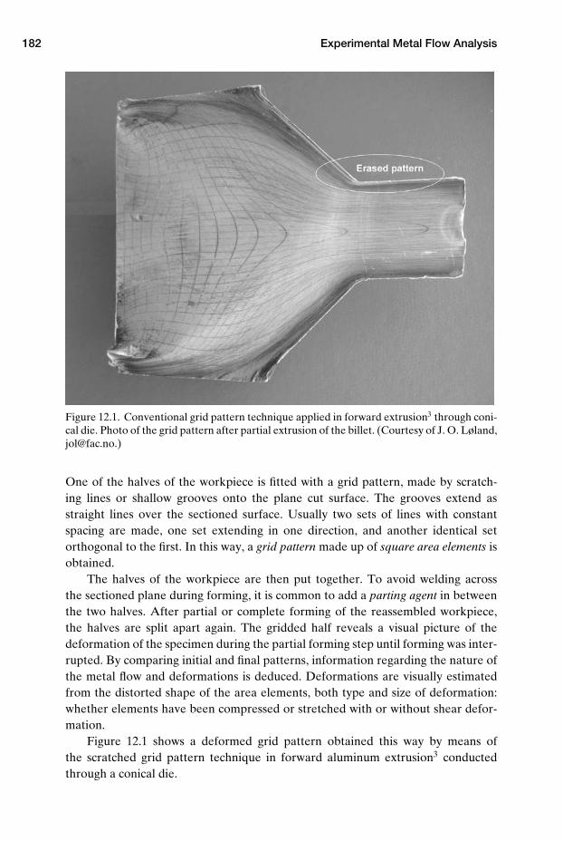
182 Experimental Metal Flow Analysis
Figure 12.1. Conventional grid pattern technique applied in forward extrusion3 through coni-cal die. Photo of the grid pattern after partial extrusion of the billet. (Courtesy of J. O. Løland,[email protected].)
One of the halves of the workpiece is fitted with a grid pattern, made by scratch-ing lines or shallow grooves onto the plane cut surface. The grooves extend asstraight lines over the sectioned surface. Usually two sets of lines with constantspacing are made, one set extending in one direction, and another identical setorthogonal to the first. In this way, a grid pattern made up of square area elements isobtained.
The halves of the workpiece are then put together. To avoid welding acrossthe sectioned plane during forming, it is common to add a parting agent in betweenthe two halves. After partial or complete forming of the reassembled workpiece,the halves are split apart again. The gridded half reveals a visual picture of thedeformation of the specimen during the partial forming step until forming was inter-rupted. By comparing initial and final patterns, information regarding the nature ofthe metal flow and deformations is deduced. Deformations are visually estimatedfrom the distorted shape of the area elements, both type and size of deformation:whether elements have been compressed or stretched with or without shear defor-mation.
Figure 12.1 shows a deformed grid pattern obtained this way by means ofthe scratched grid pattern technique in forward aluminum extrusion3 conductedthrough a conical die.
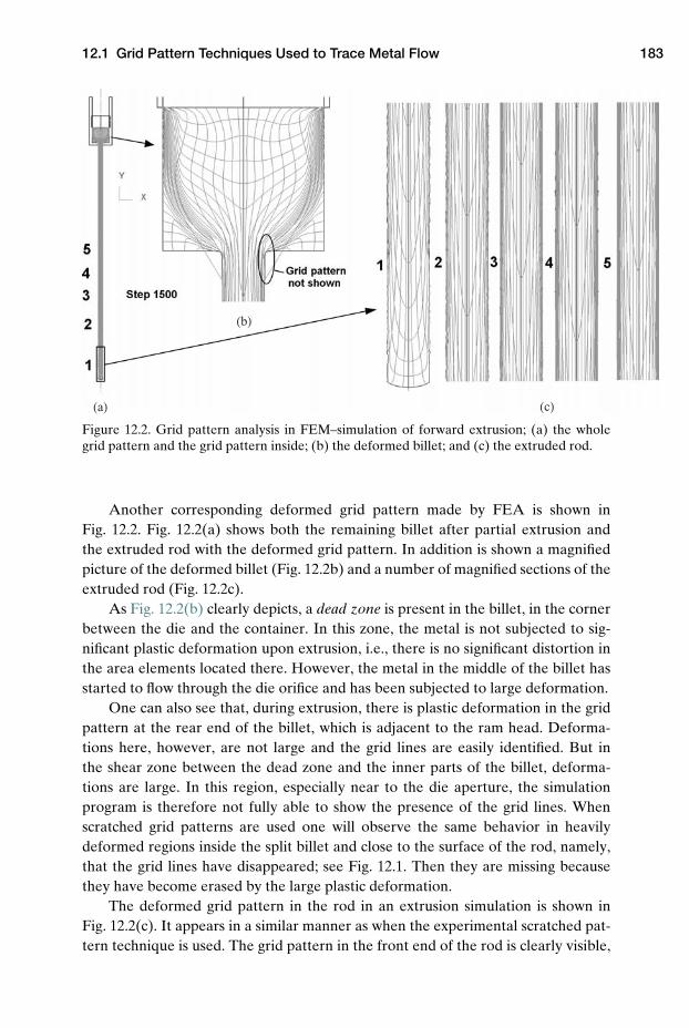
12.1 Grid Pattern Techniques Used to Trace Metal Flow 183
(a)
(b)
(c)
Figure 12.2. Grid pattern analysis in FEM–simulation of forward extrusion; (a) the wholegrid pattern and the grid pattern inside; (b) the deformed billet; and (c) the extruded rod.
Another corresponding deformed grid pattern made by FEA is shown inFig. 12.2. Fig. 12.2(a) shows both the remaining billet after partial extrusion andthe extruded rod with the deformed grid pattern. In addition is shown a magnifiedpicture of the deformed billet (Fig. 12.2b) and a number of magnified sections of theextruded rod (Fig. 12.2c).
As Fig. 12.2(b) clearly depicts, a dead zone is present in the billet, in the cornerbetween the die and the container. In this zone, the metal is not subjected to sig-nificant plastic deformation upon extrusion, i.e., there is no significant distortion inthe area elements located there. However, the metal in the middle of the billet hasstarted to flow through the die orifice and has been subjected to large deformation.
One can also see that, during extrusion, there is plastic deformation in the gridpattern at the rear end of the billet, which is adjacent to the ram head. Deforma-tions here, however, are not large and the grid lines are easily identified. But inthe shear zone between the dead zone and the inner parts of the billet, deforma-tions are large. In this region, especially near to the die aperture, the simulationprogram is therefore not fully able to show the presence of the grid lines. Whenscratched grid patterns are used one will observe the same behavior in heavilydeformed regions inside the split billet and close to the surface of the rod, namely,that the grid lines have disappeared; see Fig. 12.1. Then they are missing becausethey have become erased by the large plastic deformation.
The deformed grid pattern in the rod in an extrusion simulation is shown inFig. 12.2(c). It appears in a similar manner as when the experimental scratched pat-tern technique is used. The grid pattern in the front end of the rod is clearly visible,
184 Experimental Metal Flow Analysis
but farther away from the end, the grid pattern becomes very dense so each individ-ual grid line is not readily visible.
Conclusion is that when the scratched pattern technique is applied the tech-nique starts to fail because the grid pattern becomes erased in regions where thereare heavy deformations, as in the shear zones in the billet and in the subsurfacelayers of the extruded rod.
Another drawback of scratched grid patterns that should be mentioned is thatthey are not well suited for analysis of sliding along the die–workpiece interfaces,because they cannot be detected precisely when they extend into an interface.Because of this, such patterns do not reveal the nature of metal flow along die–workpiece interfaces with sufficient accuracy.
12.1.2 Grid Patterns Made from Contrast Pins
A modified grid pattern technique, based on introduction of a stripe pattern ofcontrast material pins into the initial billet,4,5 is often a better option than use ofscratched grid patterns. After partial extrusion such stripe pattens can be revealedand depicts the nature of metal flow, at each stage of forming, better than scratchedpatterns do. The advantage of such patterns over scratched ones is that they do notget erased – not even in heavily deformed regions as the shear zones – and hencedeformations can be investigated even there. A disadvantage is that workpieceswith internal stripe patterns are expensive to produce and to apply. But they canbe tailor-made even inside industrial-sized workpieces, and very accurate experi-ments can therefore be performed to study metal flow, on the industrial and thelaboratory scale.
Internal stripe patterns, which also can be termed intrinsic grid patterns, havebeen used with great success in deformation analysis of extrusion of aluminum.5 Thepins are inserted into holes drilled into a longitudinal symmetry plane of the initialworkpiece. Inserts of contrast alloys have been applied for a long time for studies ofmetal flow, though not in the same systematic manner as in this new variant of thetechnique, to create a complete grid pattern inside the workpiece.
When an intrinsic pattern like this is made for an AlMgSi1-alloy (AA 6082)to be hot-formed, the alloy AlCu1.8 is an appropriate contrast alloy to be used aspin material. Not only will this alloy have approximately the same flow stress as thematrix alloy, so that both will flow the same way, but, because of the Cu contentof the contrast alloy, it will turn black when etched in caustic soda or in Tucker’setchant, while the base alloy retains its bright Al color after treatment. This aggre-gate of contrast pins, after partial or complete forming, appears as a clear pattern inthe plane inside the workpiece where they are present. The workpiece is a massivebody during forming, and afterwards it must be sectioned along the plane contain-ing the pattern. The cut section is then carefully ground until it coincides with themidplane of all the pins, whereupon the pattern is “exposed” to make it visible bythe etching treatment. For the alloy AlMgSi0.5, the contrast alloy AlCu1.2 is used asmarker material. Similar patterns can also be made for other metals than aluminum,though here the focus is on applications in aluminum forming.
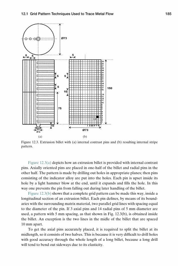
12.1 Grid Pattern Techniques Used to Trace Metal Flow 185
(a) (b)
Figure 12.3. Extrusion billet with (a) internal contrast pins and (b) resulting internal stripepattern.
Figure 12.3(a) depicts how an extrusion billet is provided with internal contrastpins. Axially oriented pins are placed in one-half of the billet and radial pins in theother half. The pattern is made by drilling out holes in appropriate planes; then pinsconsisting of the indicator alloy are put into the holes. Each pin is upset inside itshole by a light hammer blow at the end, until it expands and fills the hole. In thisway one prevents the pin from falling out during later handling of the billet.
Figure 12.3(b) shows that a complete grid pattern can be made this way, inside alongitudinal section of an extrusion billet. Each pin defines, by means of its bound-aries with the surrounding matrix material, two parallel grid lines with spacing equalto the diameter of the pin. If 3 axial pins and 14 radial pins of 5 mm diameter areused, a pattern with 5 mm spacing, as that shown in Fig. 12.3(b), is obtained insidethe billet. An exception is the two lines in the midle of the billet that are spaced10 mm apart.
To get the axial pins accurately placed, it is required to split the billet at itsmidlength, so it consists of two halves. This is because it is very difficult to drill holeswith good accuracy through the whole length of a long billet, because a long drillwill tend to bend out sideways due to its elasticity.
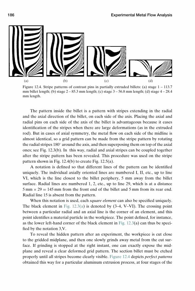
186 Experimental Metal Flow Analysis
(a) (b) (c) (d)
Figure 12.4. Stripe patterns of contrast pins in partially extruded billets: (a) stage 1 – 113.7mm billet length; (b) stage 2 – 85.3 mm length; (c) stage 3 – 56.8 mm length; (d) stage 4 – 28.4mm length.
The pattern inside the billet is a pattern with stripes extending in the radialand the axial direction of the billet, on each side of the axis. Placing the axial andradial pins on each side of the axis of the billet is advantageous because it easesidentification of the stripes when there are large deformations (as in the extrudedrod). But in cases of axial symmetry, the metal flow on each side of the midline isalmost identical, so a grid pattern can be made from the stripe pattern by rotatingthe radial stripes 180◦ around the axis, and then superposing them on top of the axialones; see Fig. 12.3(b). In this way, radial and axial stripes can be coupled togetherafter the stripe pattern has been revealed. This procedure was used on the stripepattern shown in Fig. 12.4(b) to create Fig. 12.5(a).
A notation is defined so that different lines of the pattern can be identifieduniquely. The individual axially oriented lines are numbered I, II, etc., up to lineVI, which is the line closest to the billet periphery, 5 mm away from the billetsurface. Radial lines are numbered 1, 2, etc., up to line 29, which is at a distance5 mm × 29 = 145 mm from the front end of the billet and 5 mm from its rear end.Radial line 15 is absent from the pattern.
When this notation is used, each square element can also be specified uniquely.The black element in Fig. 12.3(a) is denoted by (3–4, V–VI). The crossing pointbetween a particular radial and an axial line is the corner of an element, and thispoint identifies a material particle in the workpiece. The point defined, for instance,as the lower left-hand corner of the black element in Fig. 12.3(a) can thus be speci-fied by the notation 3,V.
To reveal the hidden pattern after an experiment, the workpiece is cut closeto the gridded midplane, and then one slowly grinds away metal from the cut sur-face. If grinding is stopped at the right instant, one can exactly expose the mid-plane and reveal a clear deformed grid pattern. The section billet must be etchedproperly until all stripes become clearly visible. Figure 12.4 depicts perfect patternsobtained this way for a particular aluminum extrusion process, at four stages of the
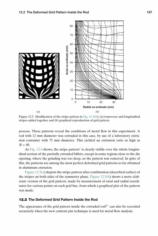
12.2 The Deformed Grid Pattern Inside the Rod 187
80
70
60
50
40
30
20
10
00 10 20 30
Radial co-ordinate (mm)
Axi
al c
o-o
rdin
ate
(mm
)
(a) (b)
Figure 12.5. Modification of the stripe pattern in Fig. 12.4(b): (a) transverse and longitudinalstripes added together and (b) graphical reproduction of grid pattern.
process. These patterns reveal the conditions of metal flow in this experiment. Arod with 12 mm diameter was extruded in this case, by use of a laboratory extru-sion container with 75 mm diameter. This yielded an extrusion ratio as high asR = 40.
As Fig. 12.4 shows, the stripe pattern6 is clearly visible over the whole longitu-dinal section of the partially extruded billets, except in some regions close to the dieopening, where the grinding was too deep, so the pattern was removed. In spite ofthis, the patterns are among the most perfect deformed grid patterns so far obtainedin aluminum extrusion.
Figure 12.5(a) depicts the stripe pattern after combination (described earlier) ofthe stripes on both sides of the symmetry plane. Figure 12.5(b) shows a more elab-orate version of the grid pattern, made by measurement of axial and radial coordi-nates for various points on each grid line, from which a graphical plot of the patternwas made.
12.2 The Deformed Grid Pattern Inside the Rod
The appearance of the grid pattern inside the extruded rod4,7 can also be recordedaccurately when the new contrast pin technique is used for metal flow analysis.
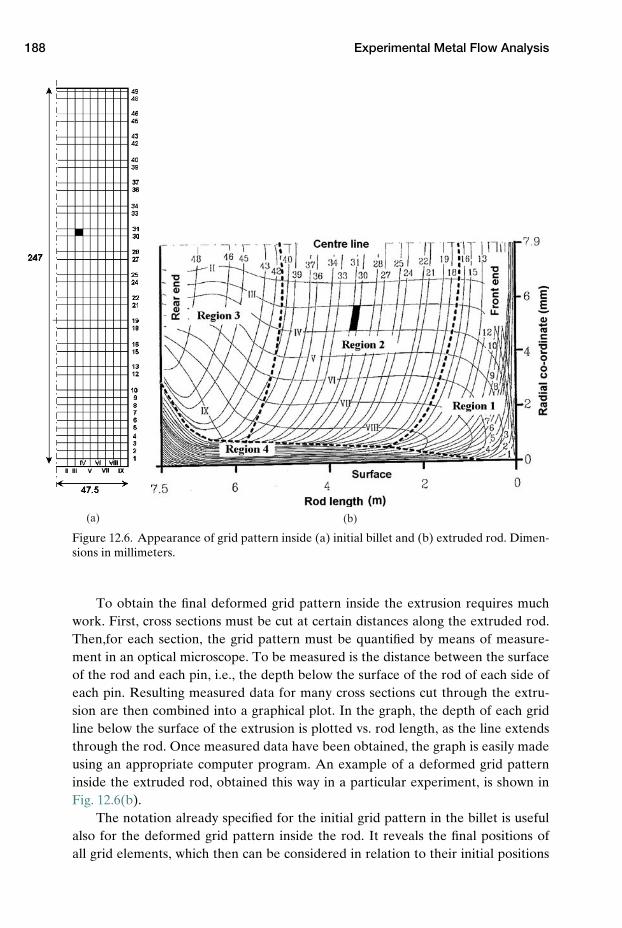
188 Experimental Metal Flow Analysis
(a) (b)
Figure 12.6. Appearance of grid pattern inside (a) initial billet and (b) extruded rod. Dimen-sions in millimeters.
To obtain the final deformed grid pattern inside the extrusion requires muchwork. First, cross sections must be cut at certain distances along the extruded rod.Then,for each section, the grid pattern must be quantified by means of measure-ment in an optical microscope. To be measured is the distance between the surfaceof the rod and each pin, i.e., the depth below the surface of the rod of each side ofeach pin. Resulting measured data for many cross sections cut through the extru-sion are then combined into a graphical plot. In the graph, the depth of each gridline below the surface of the extrusion is plotted vs. rod length, as the line extendsthrough the rod. Once measured data have been obtained, the graph is easily madeusing an appropriate computer program. An example of a deformed grid patterninside the extruded rod, obtained this way in a particular experiment, is shown inFig. 12.6(b).
The notation already specified for the initial grid pattern in the billet is usefulalso for the deformed grid pattern inside the rod. It reveals the final positions ofall grid elements, which then can be considered in relation to their initial positions
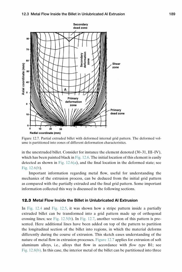
12.3 Metal Flow Inside the Billet in Unlubricated Al Extrusion 189
Figure 12.7. Partial extruded billet with deformed internal grid pattern. The deformed vol-ume is partitioned into zones of different deformation characteristics.
in the unextruded billet. Consider for instance the element denoted (30–31, III–IV),which has been painted black in Fig. 12.6. The initial location of this element is easilydetected as shown in Fig. 12.6(a), and the final location in the deformed state; seeFig. 12.6(b).
Important information regarding metal flow, useful for understanding themechanics of the extrusion process, can be deduced from the initial grid patternas compared with the partially extruded and the final grid pattern. Some importantinformation collected this way is discussed in the following sections.
12.3 Metal Flow Inside the Billet in Unlubricated Al Extrusion
In Fig. 12.4 and Fig. 12.5, it was shown how a stripe pattern inside a partiallyextruded billet can be transformed into a grid pattern made up of orthogonalcrossing lines; see Fig. 12.5(b). In Fig. 12.7, another version of this pattern is pre-sented. Here additional lines have been added on top of the pattern to partitionthe longitudinal section of the billet into regions, in which the material deformsdifferently during the course of extrusion. This sketch eases understanding of thenature of metal flow in extrusion processes. Figure 12.7 applies for extrusion of softaluminum alloys, i.e., alloys that flow in accordance with flow type B1; seeFig. 12.8(b). In this case, the interior metal of the billet can be partitioned into three
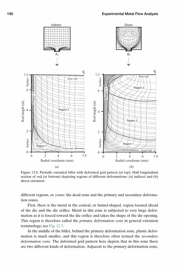
190 Experimental Metal Flow Analysis
Indirect
A1 B1
Direct
Radial coordinate (mm) Radial coordinate (mm)
Rod
leng
th (
m)
Region 2
Sur
face
Sur
face
Rod
leng
th (
m)
Sur
face
Sur
face
Rear endRear end
Front endFront end
Region 1Region 1
Reg
ion
4
Reg
ion
4
Region 2
Region 3
7.5
6
4
2
00 2 4 6 7.9
CL CL
0 2 4 6 7.9
7.5
6
4
2
0
(a) (b)
Figure 12.8. Partially extruded billet with deformed grid pattern (at top). Half longitudinalsection of rod (at bottom) depicting regions of different deformations: (a) indirect and (b)direct extrusion.
different regions, or zones: the dead zone and the primary and secondary deforma-tion zones.
First, there is the metal in the conical, or funnel-shaped, region located aheadof the die and the die orifice. Metal in this zone is subjected to very large defor-mation as it is forced toward the die orifice and takes the shape of the die opening.This region is therefore called the primary deformation zone in general extrusionterminology; see Fig. 12.7.
In the middle of the billet, behind the primary deformation zone, plastic defor-mation is much smaller, and this region is therefore often termed the secondarydeformation zone. The deformed grid pattern here depicts that in this zone thereare two different kinds of deformation. Adjacent to the primary deformation zone,

12.3 Metal Flow Inside the Billet in Unlubricated Al Extrusion 191
a number of adjacent transverse grid lines have the same characteristic convexshape. Behind this region, however, the deformation is somewhat different. Heretwo or three transverse lines close to the rear end of the billet have a double convexshape. This is because the material here encompasses the secondary dead zone onthe billet axis, adjacent to the ram head. Depending on the alloy extruded, this deadzone will be more or less well developed. It is termed secondary to distinguish itfrom the primary dead zone located ahead of the die.
The metal of the secondary deformation zone gradually flows into the primarydeformation zone. The deformation imposed on the metal while in the secondarydeformation zone can therefore be termed predeformation, in that additional largerdeformation will occur when this material, later during extrusion, flows through theprimary deformation zone.
In the peripheral region of the billet, two other zones can be identified, andthey deform differently from those in the interior of the billet. First, there is theshear zone. Because of sticking friction between billet and container wall in unlubri-cated hot extrusion of Al, the surface layers of the billet will be retained against thecontainer wall. The core of the billet, however, is pushed forward by the advancingram, and a shear zone forms between the core material, which flows forward, andthe peripheral surface layer of the billet, which sticks to the container wall. In extru-sion, this shear zone appears as a heavily deformed layer inside the billet extendingdown along the container wall. The layer of shear deformed material, due to thepresence of this zone, gradually grows in thickness throughout the course of extru-sion. Toward the die orifice, this layer bends inwards as a truncated conical layer,located in between the primary dead zone and the primary deformation zone.
Finally, ahead of the die, the billet material located in the corner region betweenthe die and the container wall is situated off from the main stream flowing throughthe die orifice, and is therefore subjected only to minor plastic deformations. Thismaterial is therefore commonly termed the primary dead zone, but sometimes alsothe elastic zone. The former term is better, because small plastic deformations dooccur in this zone.
Figure 12.7 represents the metal flow in an intermediate stage of the extru-sion process. The metal, which at this instant resides in the shear zone and in thesecondary deformation zone, sooner or later during continued extrusion will besqueezed into the primary deformation zone. It then either flows through the pri-mary deformation zone, out into the rod, or is accumulated in the discard at end ofextrusion.
When the ram has reached the horizontal line marked A in Fig. 12.7, the sec-ondary deformation zone no longer is present. With even further advancement ofthe ram, as in industrial Al extrusion, only a thin slice of metal will be left as a dis-card inside the container, ahead of the die, at the end of extrusion. When the ramstarts to penetrate into the primary deformation zone, the flow pattern completelychanges its nature. Material that prior to this instant resided in the primary deadzone will now start to deform plastically, and some of this material will also flow outinto the extrudate.
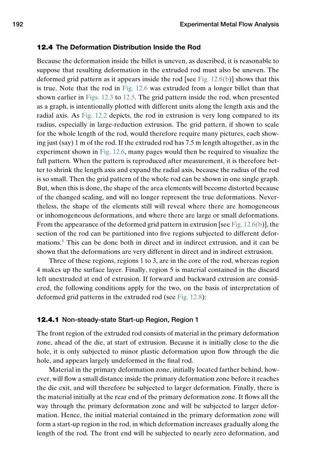
192 Experimental Metal Flow Analysis
12.4 The Deformation Distribution Inside the Rod
Because the deformation inside the billet is uneven, as described, it is reasonable tosuppose that resulting deformation in the extruded rod must also be uneven. Thedeformed grid pattern as it appears inside the rod [see Fig. 12.6(b)] shows that thisis true. Note that the rod in Fig. 12.6 was extruded from a longer billet than thatshown earlier in Figs. 12.3 to 12.5. The grid pattern inside the rod, when presentedas a graph, is intentionally plotted with different units along the length axis and theradial axis. As Fig. 12.2 depicts, the rod in extrusion is very long compared to itsradius, especially in large-reduction extrusion. The grid pattern, if shown to scalefor the whole length of the rod, would therefore require many pictures, each show-ing just (say) 1 m of the rod. If the extruded rod has 7.5 m length altogether, as in theexperiment shown in Fig. 12.6, many pages would then be required to visualize thefull pattern. When the pattern is reproduced after measurement, it is therefore bet-ter to shrink the length axis and expand the radial axis, because the radius of the rodis so small. Then the grid pattern of the whole rod can be shown in one single graph.But, when this is done, the shape of the area elements will become distorted becauseof the changed scaling, and will no longer represent the true deformations. Never-theless, the shape of the elements still will reveal where there are homogeneousor inhomogeneous deformations, and where there are large or small deformations.From the appearance of the deformed grid pattern in extrusion [see Fig. 12.6(b)], thesection of the rod can be partitioned into five regions subjected to different defor-mations.8 This can be done both in direct and in indirect extrusion, and it can beshown that the deformations are very different in direct and in indirect extrusion.
Three of these regions, regions 1 to 3, are in the core of the rod, whereas region4 makes up the surface layer. Finally, region 5 is material contained in the discardleft unextruded at end of extrusion. If forward and backward extrusion are consid-ered, the following conditions apply for the two, on the basis of interpretation ofdeformed grid patterns in the extruded rod (see Fig. 12.8):
12.4.1 Non-steady-state Start-up Region, Region 1
The front region of the extruded rod consists of material in the primary deformationzone, ahead of the die, at start of extrusion. Because it is initially close to the diehole, it is only subjected to minor plastic deformation upon flow through the diehole, and appears largely undeformed in the final rod.
Material in the primary deformation zone, initially located farther behind, how-ever, will flow a small distance inside the primary deformation zone before it reachesthe die exit, and will therefore be subjected to larger deformation. Finally, there isthe material initially at the rear end of the primary deformation zone. It flows all theway through the primary deformation zone and will be subjected to larger defor-mation. Hence, the initial material contained in the primary deformation zone willform a start-up region in the rod, in which deformation increases gradually along thelength of the rod. The front end will be subjected to nearly zero deformation, and

12.4 The Deformation Distribution Inside the Rod 193
then there will be increasing deformation, building up to large values at the otherend of the start-up region of the rod. Moreover, the size of these deformations willincrease if the reduction ratio in the process is increased.
Forward extrusion yields a primary deformation zone of greater thickness thanbackward extrusion. The non-steady-state start-up region, region 1, as depicted inFig. 12.8, therefore is present in a larger part of the rod in direct than in indirectextrusion.
12.4.2 Steady-state Region, Region 2
The material in the core of the billet, initially located behind the primary defor-mation zone, is subjected to small predeformation as it flows toward the primarydeformation zone. Later, it is subjected to additional large deformation during flowthrough the primary deformation zone. The same applies to the rest of the materialinitially in the secondary deformation zone.
Because of this, there is a region in the rod that experiences almost steady-statedeformation. This region is denoted as region 2 in Fig. 12.8, and occurs directlybehind region 1. The deformation in this region is approximately constant along thelength of the rod, but increases from the center toward the surface, as it also does inregions 1 and 3. In indirect extrusion this steady-state region extends deep into therod, whereas in direct extrusion a second well-developed non-steady-state region,region 3, appears toward the rear end of the rod.
12.4.3 Non-steady-state Back End Region, Region 3
Both in direct and in indirect extrusion there is a non-steady-state region behind thesteady-state region of the rod, in which the deformation increases over that experi-enced in the steady-state region; see Fig. 12.8.
In direct extrusion, the increased deformation experienced by material in therear end of the rod is due to two different phenomena. First, there is the scrap-ing action of the ram against the container wall during the course of extrusion. Theretained peripheral layer of the billet being scraped off by the ram head is forcedto flow inward in the radial direction, in the rear end of the billet. Because of this,the rear billet end is strongly predeformed prior to its entry into the primary defor-mation zone. The deformation at the rear end of the billet is therefore the sum ofthe scraping predeformation and later deformation during flow through the primarydeformation zone.
The other phenomenon occurs when the ram approaches the die, for it thenstarts to push out the dead zone ahead of the die. Prior to this, the dead zoneremains largely stationary adjacent to the die. When the ram head approaches thedead zones, they start to deform, and dead zone material flows in the radial directioninward into the billet, causing further radial compression of the core of the billet.
Both flow phenomena occur concurrently in the end phase of extrusion, so theradial compression of the rear billet end is due to their combined effects.
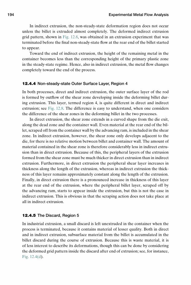
194 Experimental Metal Flow Analysis
In indirect extrusion, the non-steady-state deformation region does not occurunless the billet is extruded almost completely. The deformed indirect extrusiongrid pattern, shown in Fig. 12.8, was obtained in an extrusion experiment that wasterminated before the final non-steady-state flow at the rear end of the billet startedto appear.
Toward the end of indirect extrusion, the height of the remaining metal in thecontainer becomes less than the corresponding height of the primary plastic zonein the steady-state regime. Hence, also in indirect extrusion, the metal flow changescompletely toward the end of the process.
12.4.4 Non-steady-state Outer Surface Layer, Region 4
In both processes, direct and indirect extrusion, the outer surface layer of the rodis formed by outflow of the shear zone developing inside the deforming billet dur-ing extrusion. This layer, termed region 4, is quite different in direct and indirectextrusion; see Fig. 12.8. The difference is easy to understand, when one considersthe difference of the shear zones in the deforming billet in the two processes.
In direct extrusion, the shear zone extends in a curved shape from the die exit,along the dead zone and the container wall. Even material at the rear end of the bil-let, scraped off from the container wall by the advancing ram, is included in the shearzone. In indirect extrusion, however, the shear zone only develops adjacent to thedie, for there is no relative motion between billet and container wall. The amount ofmaterial contained in the shear zone is therefore considerably less in indirect extru-sion than in direct extrusion. Because of this, the peripheral layers of the extrusionformed from the shear zone must be much thicker in direct extrusion than in indirectextrusion. Furthermore, in direct extrusion the peripheral shear layer increases inthickness along the length of the extrusion, whereas in indirect extrusion the thick-ness of this layer remains approximately constant along the length of the extrusion.Finally, in direct extrusion there is a pronounced increase in thickness of this layerat the rear end of the extrusion, where the peripheral billet layer, scraped off bythe advancing ram, starts to appear inside the extrusion, but this is not the case inindirect extrusion. This is obvious in that the scraping action does not take place atall in indirect extrusion.
12.4.5 The Discard, Region 5
In industrial extrusion, a small discard is left unextruded in the container when theprocess is terminated, because it contains material of lesser quality. Both in directand in indirect extrusion, subsurface material from the billet is accumulated in thebillet discard during the course of extrusion. Because this is waste material, it isof less interest to describe its deformations, though this can be done by consideringthe deformed grid pattern inside the discard after end of extrusion; see, for instance,Fig. 12.4(d).
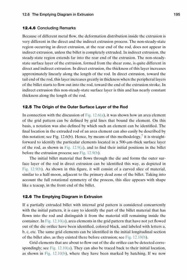
12.6 The Emptying Diagram in Extrusion 195
12.4.6 Concluding Remarks
Because of different metal flow, the deformation distribution inside the extrusion isvery different in the direct and the indirect extrusion process. The non-steady-stateregion occurring in direct extrusion, at the rear end of the rod, does not appear inindirect extrusion, unless the billet is completely extruded. In indirect extrusion, thesteady-state region extends far into the rear end of the extrusion. The non-steady-state surface layer of the extrusion, formed from the shear zone, is quite different indirect and indirect extrusion. In direct extrusion, the thickness of this layer increasesapproximately linearly along the length of the rod. In direct extrusion, toward thetail end of the rod, this layer increases greatly in thickness when the peripheral layersof the billet starts to flow out into the rod, toward the end of the extrusion stroke. Inindirect extrusion this non-steady-state surface layer is thin and has nearly constantthickness along the length of the rod.
12.5 The Origin of the Outer Surface Layer of the Rod
In connection with the discussion of Fig. 12.6(a), it was shown how an area elementof the grid pattern can be defined by grid lines that bound the element. On thisbasis, a notation was also defined by which such an element can be identified. Thefinal location in the extruded rod of an area element can also easily be described bythis notation; see Fig. 12.6(b). Hence, by means of this methodology,7 it is straight-forward to identify the particular elements located in a 500-µm-thick surface layerof the rod, as shown in Fig. 12.9(a), and to find their initial positions in the billetbefore the extrusion process; see Fig. 12.9(b).
The initial billet material that flows through the die and forms the outer sur-face layer of the rod in direct extrusion can be identified this way, as depicted inFig. 12.9(b). As shown in this figure, it will consist of a curved slice of material,similar to a half-moon, adjacent to the primary dead zone of the billet. Taking intoaccount the full rotational symmetry of the process, this slice appears with shapelike a teacup, in the front end of the billet.
12.6 The Emptying Diagram in Extrusion
If a partially extruded billet with internal grid pattern is considered concurrentlywith the initial pattern, it is easy to identify the part of the billet material that hasflown into the rod and distinguish it from the material still remaining inside thecontainer. In Fig. 12.10(a), area elements in the grid pattern that have not yet flowedout of the die orifice have been identified, colored black, and labeled with letters a,b, c, etc. The same grid elements can be identified in the initial longitudinal sectionof the billet also, as they existed there before extrusion; see Fig. 12.10(b).
Grid elements that are about to flow out of the die orifice can be detected corre-spondingly; see Fig. 12.10(a). They can also be traced back to their initial location,as shown in Fig. 12.10(b), where they have been marked by hatching. If we now
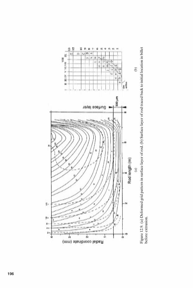
(a)
(b)
Fig
ure
12.9
.(a
)D
efor
med
grid
patt
ern
insu
rfac
ela
yer
ofro
d.(b
)Su
rfac
ela
yer
ofro
dtr
aced
back
toin
itia
lloc
atio
nin
bille
tbe
fore
extr
usio
n.
196
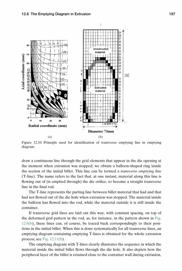
12.6 The Emptying Diagram in Extrusion 197
(a) (b)
Figure 12.10. Principle used for identification of transverse emptying line in emptyingdiagram.
draw a continuous line through the grid elements that appear in the die opening atthe moment when extrusion was stopped, we obtain a balloon-shaped ring insidethe section of the initial billet. This line can be termed a transverse emptying line(T-line). The name refers to the fact that, at one instant, material along this line isflowing out of (is emptied through) the die orifice, to become a straight transverseline in the final rod.
The T-line represents the parting line between billet material that had and thathad not flowed out of the die hole when extrusion was stopped. The material insidethe balloon has flowed into the rod, while the material outside it is still inside thecontainer.
If transverse grid lines are laid out this way, with constant spacing, on top ofthe deformed grid pattern in the rod, as, for instance, in the pattern shown in Fig.12.6(b), these lines can, of course, be traced back correspondingly to their posi-tions in the initial billet. When this is done systematically for all transverse lines, anemptying diagram containing emptying T-lines is obtained for the whole extrusionprocess; see Fig. 12.11(b).
The emptying diagram with T-lines clearly illustrates the sequence in which thematerial inside the initial billet flows through the die hole. It also depicts how theperipheral layer of the billet is retained close to the container wall during extrusion,
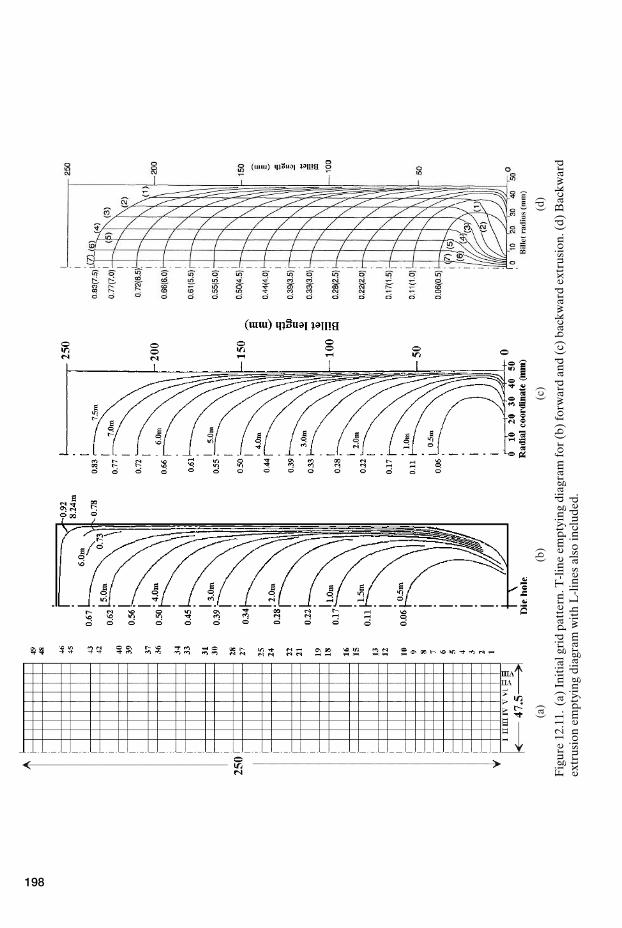
(a)
(b)
(c)
(d)
Fig
ure
12.1
1.(a
)In
itia
lgri
dpa
tter
n.T
-lin
eem
ptyi
ngdi
agra
mfo
r(b
)fo
rwar
dan
d(c
)ba
ckw
ard
extr
usio
n.(d
)B
ackw
ard
extr
usio
nem
ptyi
ngdi
agra
mw
ith
L-l
ines
also
incl
uded
.
198

12.7 Surface Ring Patterns to Trace Friction 199
P1 P2 P3 P4
P1 P2 P3 P4
P1 P2 P3 P4
Step - 1
Step 250
Step 100
0
5
10
15
20
25
30
35
0 1 2 3 4Point no.
Rad
ial d
ista
nce (
mm
)
m = 0m = 0.1m = 0.2m = 0.3m = 0.4m = 0.6m = 0.8m = 1.0Sticking
K = 150, n = 0.15
(a) (b)
Figure 12.12. (a) Sliding movement of marker points over the end face of a cylinder in com-pression, m = 0.65. (b) Graphical presentation of friction dependence.
due to sticking friction on this wall. Because of this, the outer layer of the billet alsoaccumulates in the billet discard during extrusion.
The T-line emptying diagram obtained in forward extrusion of the gridded billetin 12.11(a) is shown in Fig. 12.11(b). A corresponding diagram for indirect extrusionis shown in Fig. 12.11(c). Comparison of the two diagrams reveals that in backwardextrusion, there is a much stronger tendency for the peripheral layer of the billet toflow out into the rod than in forward extrusion.
Using a corresponding principle, longitudinal (L) emptying lines can also bemade. A full emptying diagram7 can finally be obtained by merging of T and L lines.Figure 12.11(d) shows an emptying diagram for indirect extrusion where both T andL emptying lines are shown.
12.7 Surface Ring Patterns to Trace Friction
In connection with Fig. 3.6, it was shown how an experimental surface ring patterncan be used for the purpose of determining friction in a metal forming operation.Friction between die and workpiece was in this connection determined by inversemodeling. The pattern was used to trace the movement and the stretching of theouter surface layer of the workpiece against the die, in order to find the numer-ical value of the friction factor by means of a FEM model of the actual formingoperation.
In addition, such rings can be applied on surfaces that deform plastically to tracelarge surface deformations. The methodology can be applied in any laboratory, orin industrial metal forming applications, but requires that an accurate FEM modelof the forming process be available. In the following paragraphs, the use of thistechnique for determining friction in cylinder compression will be outlined.
First, let us consider the friction dependence of the flow of the end face of acylinder compressed between plane-parallel platens. In Fig. 12.12(a), it is shown
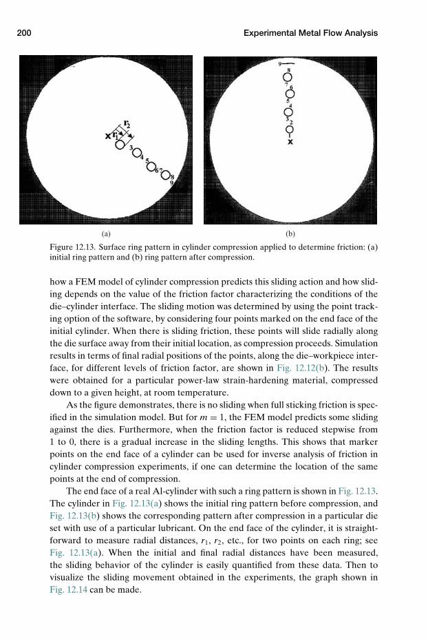
200 Experimental Metal Flow Analysis
(a) (b)
Figure 12.13. Surface ring pattern in cylinder compression applied to determine friction: (a)initial ring pattern and (b) ring pattern after compression.
how a FEM model of cylinder compression predicts this sliding action and how slid-ing depends on the value of the friction factor characterizing the conditions of thedie–cylinder interface. The sliding motion was determined by using the point track-ing option of the software, by considering four points marked on the end face of theinitial cylinder. When there is sliding friction, these points will slide radially alongthe die surface away from their initial location, as compression proceeds. Simulationresults in terms of final radial positions of the points, along the die–workpiece inter-face, for different levels of friction factor, are shown in Fig. 12.12(b). The resultswere obtained for a particular power-law strain-hardening material, compresseddown to a given height, at room temperature.
As the figure demonstrates, there is no sliding when full sticking friction is spec-ified in the simulation model. But for m = 1, the FEM model predicts some slidingagainst the dies. Furthermore, when the friction factor is reduced stepwise from1 to 0, there is a gradual increase in the sliding lengths. This shows that markerpoints on the end face of a cylinder can be used for inverse analysis of friction incylinder compression experiments, if one can determine the location of the samepoints at the end of compression.
The end face of a real Al-cylinder with such a ring pattern is shown in Fig. 12.13.The cylinder in Fig. 12.13(a) shows the initial ring pattern before compression, andFig. 12.13(b) shows the corresponding pattern after compression in a particular dieset with use of a particular lubricant. On the end face of the cylinder, it is straight-forward to measure radial distances, r1, r2, etc., for two points on each ring; seeFig. 12.13(a). When the initial and final radial distances have been measured,the sliding behavior of the cylinder is easily quantified from these data. Then tovisualize the sliding movement obtained in the experiments, the graph shown inFig. 12.14 can be made.
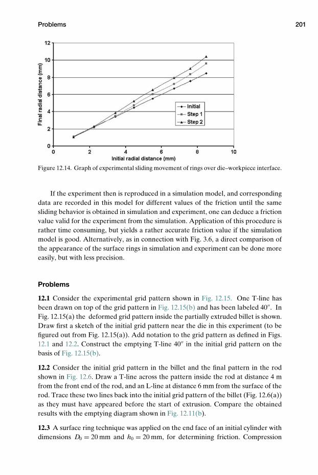
Problems 201
Figure 12.14. Graph of experimental sliding movement of rings over die–workpiece interface.
If the experiment then is reproduced in a simulation model, and correspondingdata are recorded in this model for different values of the friction until the samesliding behavior is obtained in simulation and experiment, one can deduce a frictionvalue valid for the experiment from the simulation. Application of this procedure israther time consuming, but yields a rather accurate friction value if the simulationmodel is good. Alternatively, as in connection with Fig. 3.6, a direct comparison ofthe appearance of the surface rings in simulation and experiment can be done moreeasily, but with less precision.
Problems
12.1 Consider the experimental grid pattern shown in Fig. 12.15. One T-line hasbeen drawn on top of the grid pattern in Fig. 12.15(b) and has been labeled 40′′. InFig. 12.15(a) the deformed grid pattern inside the partially extruded billet is shown.Draw first a sketch of the initial grid pattern near the die in this experiment (to befigured out from Fig. 12.15(a)). Add notation to the grid pattern as defined in Figs.12.1 and 12.2. Construct the emptying T-line 40′′ in the initial grid pattern on thebasis of Fig. 12.15(b).
12.2 Consider the initial grid pattern in the billet and the final pattern in the rodshown in Fig. 12.6. Draw a T-line across the pattern inside the rod at distance 4 mfrom the front end of the rod, and an L-line at distance 6 mm from the surface of therod. Trace these two lines back into the initial grid pattern of the billet (Fig. 12.6(a))as they must have appeared before the start of extrusion. Compare the obtainedresults with the emptying diagram shown in Fig. 12.11(b).
12.3 A surface ring technique was applied on the end face of an initial cylinder withdimensions D0 = 20 mm and h0 = 20 mm, for determining friction. Compression
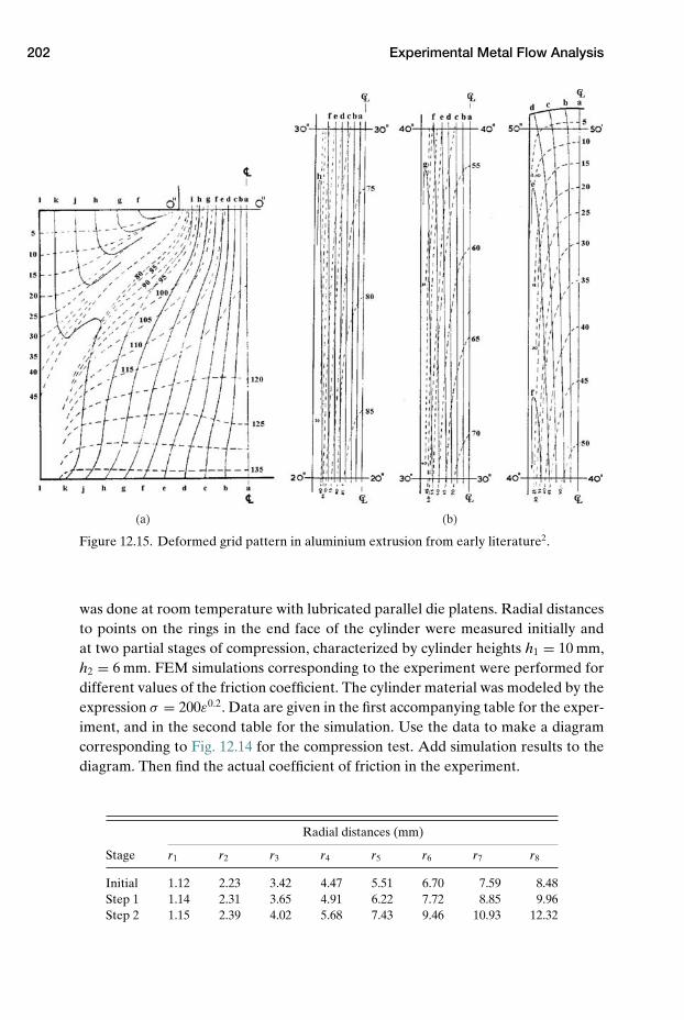
202 Experimental Metal Flow Analysis
(a) (b)
Figure 12.15. Deformed grid pattern in aluminium extrusion from early literature2.
was done at room temperature with lubricated parallel die platens. Radial distancesto points on the rings in the end face of the cylinder were measured initially andat two partial stages of compression, characterized by cylinder heights h1 = 10 mm,h2 = 6 mm. FEM simulations corresponding to the experiment were performed fordifferent values of the friction coefficient. The cylinder material was modeled by theexpression σ = 200ε0.2. Data are given in the first accompanying table for the exper-iment, and in the second table for the simulation. Use the data to make a diagramcorresponding to Fig. 12.14 for the compression test. Add simulation results to thediagram. Then find the actual coefficient of friction in the experiment.
Radial distances (mm)
Stage r1 r2 r3 r4 r5 r6 r7 r8
Initial 1.12 2.23 3.42 4.47 5.51 6.70 7.59 8.48Step 1 1.14 2.31 3.65 4.91 6.22 7.72 8.85 9.96Step 2 1.15 2.39 4.02 5.68 7.43 9.46 10.93 12.32
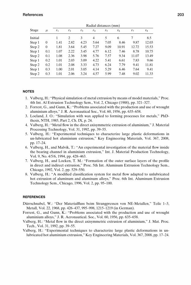
References 203
Radial distances (mm)Stage µ r1 r2 r3 r4 r5 r6 r7 r8
Initial 1 2 3 4 5 6 7 8.5Step 1 0 1.41 2.82 4.23 5.64 7.05 8.46 9.87 12.03Step 2 0 1.81 3.64 5.45 7.27 9.09 10.91 12.72 15.53Step 1 0.1 1.07 2.22 3.45 4.77 6.12 7.46 8.78 10.75Step 2 0.1 1.08 2.36 3.98 5.76 7.57 9.34 11.07 13.49Step 1 0.2 1.01 2.03 3.09 4.22 5.41 6.61 7.83 9.66Step 2 0.2 1.01 2.08 3.33 4.73 6.24 7.79 9.41 11.81Step 1 0.3 1.00 2.01 3.05 4.14 5.29 6.46 7.64 9.41Step 2 0.3 1.01 2.06 3.24 4.57 5.99 7.48 9.02 11.33
NOTES
1. Valberg, H.: “Physical simulation of metal extrusion by means of model materials,” Proc.4th Int. Al Extrusion Technology Sem., Vol. 2, Chicago (1988), pp. 321–327.
2. Forrest, G., and Gunn, K.: “Problems associated with the production and use of wroughtaluminium alloys,” J. R. Aeronautical Soc., Vol. 60, 1956, pp. 635–658.
3. Loeland, J. O.: “Simulation with wax applied to forming processes for metals,” PhD-thesis, NTH, 1985, Part 2, Ch. IX, p. 24.
4. Valberg, H.: “Metal flow in the direct axisymmetric extrusion of aluminium,” J. MaterialProcessing Technology, Vol. 31, 1992, pp. 39–55.
5. Valberg, H.: “Experimental techniques to characterize large plastic deformations inun-lubricated hot aluminium extrusion,” Key Engineering Materials, Vol. 367, 2008,pp. 17–24.
6. Valberg, H., and Malvik, T.: “An experimental investigation of the material flow insidethe bearing channel in aluminium extrusion,” Int. J. Material Production Technology,Vol. 9, No. 4/5/6, 1994, pp. 428–463.
7. Valberg, H., and Loeken, T. M.: “Formation of the outer surface layers of the profilein direct and indirect extrusion,” Proc. 5th Int. Aluminum Extrusion Technology Sem.,Chicago, 1992, Vol. 2, pp. 529–550.
8. Valberg, H.: “A modified classification system for metal flow adapted to unlubricatedhot extrusion of aluminum and aluminum alloys,” Proc. 6th Int. Aluminum ExtrusionTechnology Sem., Chicago, 1996, Vol. 2, pp. 95–100.
REFERENCES
Durrschnabel, W.: “Der Materialfluss beim Strangpressen von NE-Metallen,” Teile 1–3,Metall, Vol. 22, 1968, pp. 426–437, 995–998, 1215–1219 (in German).
Forrest, G., and Gunn, K.: “Problems associated with the production and use of wroughtaluminium alloys,” J. R. Aeronautical. Soc., Vol. 60, 1956, pp. 635–658.
Valberg, H.: “Metal flow in the direct axisymmetric extrusion of aluminium,” J. Mat. Proc.Tech., Vol. 31, 1992, pp. 39–55.
Valberg, H.: “Experimental techniques to characterize large plastic deformations in un-lubricated hot aluminium extrusion,” Key Engineering Materials, Vol. 367, 2008, pp. 17–24.
13 Theoretical Methods of Analysis
It is important – as shown in the preceding chapters – to be able to predict thedeformations and the metal flow in metal forming with sufficient accuracy. Theimportance of knowing such factors as the pressure against the die and the requiredforming load was early recognized by the metal former. Much work was thereforedone to develop theoretical models that could be used to predict these parameters,so that they could be estimated with sufficient accuracy before a new process wasset up. The theoretical models established for this purpose showed that the formingload depended on such factors as die geometry and friction, for instance, and in hotforming also on the forming speed. With the development of theoretical methods,it also became possible to calculate the effect of each factor on the forming load.
There are a number of theoretical methods that can be used for analyzing metalforming processes; see Table 13.1.1 In the following sections, they will be described,except for the slip line field and the finite difference methods, which have beendescribed elsewhere.2 The information that can be obtained by the different meth-ods is specified in Table 13.1. Additional written material that describes the appli-cation of the slip line theory for analysis of metal forming and compares it withcorresponding analysis by FEA is available at www.cambridge.org/valberg.
13.1 The Uniform Energy Method
The uniform energy method is the simplest method. It is sometimes also called theideal work method because it considers ideal frictionless homogeneous deformationof the workpiece. It is based on setting up an energy balance, where the energyused in the forming operation is calculated, neglecting the effects of friction andinhomogeneous deformation. In Ch. 18.11.1, eq. 18-3, it is shown, for instance, howthe required force in axisymmetric extrusion can be partitioned into four parts. Thesecond part is denoted by the symbol Fdh, and is the force required if the materialdeforms homogeneously in the extrusion process. In Ch. 18.11.3, this second part isdetermined by means of the slab method; see eq. 18-17.
By use of the uniform energy method, we can obtain Fdh in a much simpler way.Consider a round billet being reduced by extrusion from initial cross section A0 to
204
13.2 The Slab Method 205
Table 13.1. Theoretical methods of analysis used in metal forming
Analysis results
Method Velocity field Stress field Temperature field Stresses on tooling
Uniform energy xSlab x xUpper-bound x xSlip line field x x xFinite element x x x xFinite difference x x x x
a rod of final cross section A1. The deformation energy required to transform thisbillet into a rod can be computed by use of either eq. 4-44 or eq. 4-46 in Ch. 4. Useof the latter yields
W = VU = V∫ εb
εa
σdε = Vσ
∫ εb
εa
dε = Vσ (εa − εa)
Vσ (εa − εa) = A0lσ ε = A0lσ · ln(
A0
A1
)= Fdhl
We have now obtained the same result as that found by the slab method (eq.18-17), i.e.,
Fdh = πr20 σ ln
A0
A1= A0σ ln
A0
A1(13-1)
13.2 The Slab Method
This method will be described by demonstrating the use of it in the case of planestrain compression. Consider such compression with overhanging flat die platens;see the sketch in Fig. 13.1. The slab method 3–6 is based on setting up a force balancefor a small slab element inside the deformation zone of the workpiece. The equa-tions obtained this way are thereafter developed further, until an expression for thestress distribution inside the workpiece is obtained. The distribution of contact pres-sure over the die–workpiece interface is then estimated, and from this is obtainedthe force required by the die to compress the object.
13.2.1 The Slab Method in Plane Strain Compression with Tresca Friction
Consider the compression process shown in Fig. 13.1(a), where there is no metalflow in the direction normal to the plane of the paper. A longitudinal half sec-tion of the specimen has been redrawn in Fig. 13.1(b). A slab element inside thehalf section has also been indicated, and stress components on the element areshown.
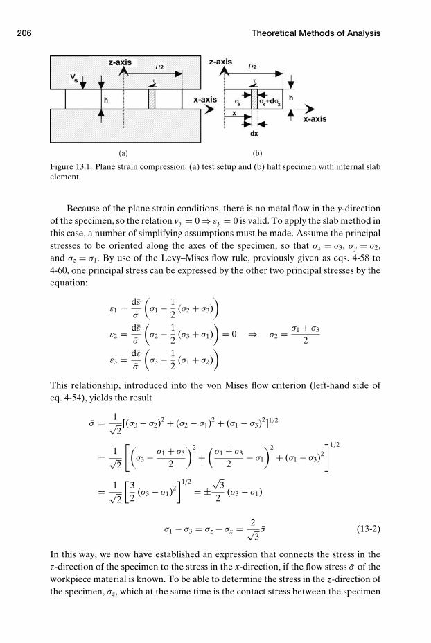
206 Theoretical Methods of Analysis
(a) (b)
Figure 13.1. Plane strain compression: (a) test setup and (b) half specimen with internal slabelement.
Because of the plane strain conditions, there is no metal flow in the y-directionof the specimen, so the relation vy = 0 ⇒ εy = 0 is valid. To apply the slab method inthis case, a number of simplifying assumptions must be made. Assume the principalstresses to be oriented along the axes of the specimen, so that σx = σ3, σy = σ2,and σz = σ1. By use of the Levy–Mises flow rule, previously given as eqs. 4-58 to4-60, one principal stress can be expressed by the other two principal stresses by theequation:
ε1 = dε
σ
(σ1 − 1
2(σ2 + σ3)
)
ε2 = dε
σ
(σ2 − 1
2(σ3 + σ1)
)= 0 ⇒ σ2 = σ1 + σ3
2
ε3 = dε
σ
(σ3 − 1
2(σ1 + σ2)
)
This relationship, introduced into the von Mises flow criterion (left-hand side ofeq. 4-54), yields the result
σ = 1√2
[(σ3 − σ2)2 + (σ2 − σ1)2 + (σ1 − σ3)2]1/2
= 1√2
[(σ3 − σ1 + σ3
2
)2
+(
σ1 + σ3
2− σ1
)2
+ (σ1 − σ3)2
]1/2
= 1√2
[32
(σ3 − σ1)2]1/2
= ±√
32
(σ3 − σ1)
σ1 − σ3 = σz − σx = 2√3σ (13-2)
In this way, we now have established an expression that connects the stress in thez-direction of the specimen to the stress in the x-direction, if the flow stress σ of theworkpiece material is known. To be able to determine the stress in the z-direction ofthe specimen, σz, which at the same time is the contact stress between the specimen

13.2 The Slab Method 207
and the die, it is required to establish an additional equation between the two prin-cipal stresses σz and σx. This equation is obtained by considering force balance forthe hatched slab element shown in Fig. 13.1(b). The whole specimen, and the slabelement considered, are assumed to have dimension equal to unity in the directionorthogonal to the paper plane, i.e., in the y-direction.
Consider the specimen when it has been compressed down to a thickness h frominitial thickness h0. Assume the stress in the x-direction to increase by the amountdσx from the initial position x to a new position the incremental distance dx fur-ther to the right. Then the following force balance can be established for the slabelement: ∑
Fx = σxh · 1 − (σx + dσx) h · 1 − 2τ dx · 1 = 0
The force contribution 2τ dx · 1 is the friction force created because the slab ele-ment slides laterally away from the neutral plane of the specimen during the strokeof compression. From the force equilibrium, the following differential equation isobtained: ∫
dσx =∫
−2τ
hdx
After integration this expression yields
σx = −2τ
hx + C (13-3)
The constant C is determined by considering known boundary conditions. At theedge of the specimen, i.e., for x = l/2, the stress in the x-direction must be σx = 0,because a surface without tool contact is stress-free in the direction orthogonal tothe surface. Introduction of this relationship into eq. 13-3 gives the following inte-gration constant:
0 = −2τ
hl2
+ C ⇒ C = τ
hl
The constant C is now eliminated from eq. 13-3, with the following result:
σx = −2τ
hx + τ l
h(13-4)
It is now straightforward to express the stress component σz in term of known pro-cess parameters, by combining of the two equations 13-2 and 13-4:
σz = σx + 2√3σ = −2τ
hx + τ l
h+ 2√
3σ = 2τ
h
(l2
− x)
+ 2√3σ (13-5)
If we assume Tresca friction, the expression τ = mσ /√
3 (see eq. 10-8) can be intro-duced to give the equation
σz = 2mσ√3 · h
(l2
− x)
+ 2√3σ (13-6)
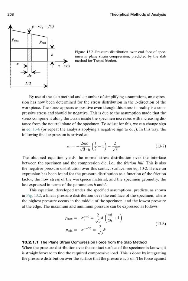
208 Theoretical Methods of Analysis
Figure 13.2. Pressure distribution over end face of spec-imen in plane strain compression, predicted by the slabmethod for Tresca friction.
By use of the slab method and a number of simplifying assumptions, an expres-sion has now been determined for the stress distribution in the z-direction of theworkpiece. The stress appears as positive even though this stress in reality is a com-pressive stress and should be negative. This is due to the assumption made that thestress component along the x-axis inside the specimen increases with increasing dis-tance from the neutral plane of the specimen. To adjust for this, we can change signin eq. 13-6 (or repeat the analysis applying a negative sign to dσx). In this way, thefollowing final expression is arrived at:
σz = − 2mσ√3 · h
(l2
− x)
− 2√3σ (13-7)
The obtained equation yields the normal stress distribution over the interfacebetween the specimen and the compression die, i.e., the friction hill. This is alsothe negative pressure distribution over this contact surface; see eq. 10-2. Hence anexpression has been found for the pressure distribution as a function of the frictionfactor, the flow stress of the workpiece material, and the specimen geometry, thelast expressed in terms of the parameters h and l.
This equation, developed under the specified assumptions, predicts, as shownin Fig. 13.2, a linear pressure distribution over the end face of the specimen, wherethe highest pressure occurs in the middle of the specimen, and the lowest pressureat the edge. The maximum and minimum pressure can be expressed as follows:
pmax = −σ x=0z = 2√
3σ
(ml2h
+ 1)
(13-8)pmin = −σ x=l/2
z = 2√3σ
13.2.1.1 The Plane Strain Compression Force from the Slab MethodWhen the pressure distribution over the contact surface of the specimen is known, itis straightforward to find the required compressive load. This is done by integratingthe pressure distribution over the surface that the pressure acts on. The force against
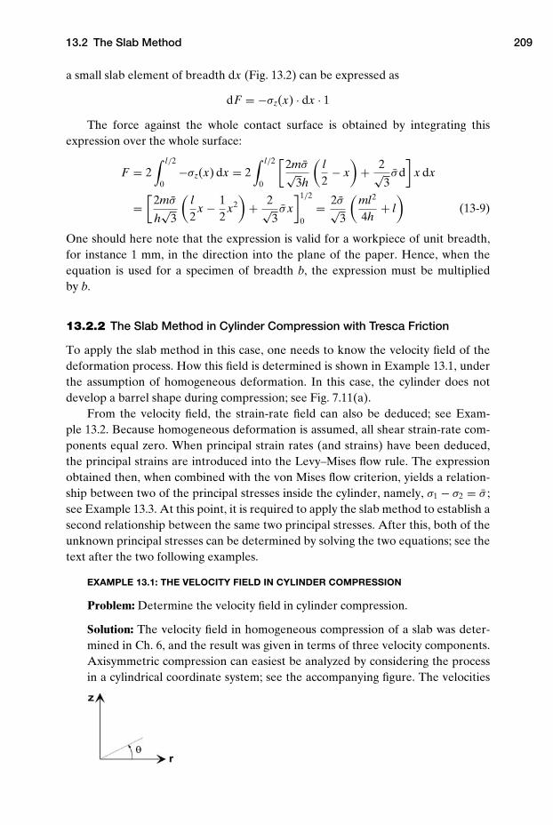
13.2 The Slab Method 209
a small slab element of breadth dx (Fig. 13.2) can be expressed as
dF = −σz(x) · dx · 1
The force against the whole contact surface is obtained by integrating thisexpression over the whole surface:
F = 2∫ l/2
0−σz(x) dx = 2
∫ l/2
0
[2mσ√
3h
(l2
− x)
+ 2√3σd
]x dx
=[
2mσ
h√
3
(l2
x − 12
x2)
+ 2√3σ x
]1/2
0= 2σ√
3
(ml2
4h+ l
)(13-9)
One should here note that the expression is valid for a workpiece of unit breadth,for instance 1 mm, in the direction into the plane of the paper. Hence, when theequation is used for a specimen of breadth b, the expression must be multipliedby b.
13.2.2 The Slab Method in Cylinder Compression with Tresca Friction
To apply the slab method in this case, one needs to know the velocity field of thedeformation process. How this field is determined is shown in Example 13.1, underthe assumption of homogeneous deformation. In this case, the cylinder does notdevelop a barrel shape during compression; see Fig. 7.11(a).
From the velocity field, the strain-rate field can also be deduced; see Exam-ple 13.2. Because homogeneous deformation is assumed, all shear strain-rate com-ponents equal zero. When principal strain rates (and strains) have been deduced,the principal strains are introduced into the Levy–Mises flow rule. The expressionobtained then, when combined with the von Mises flow criterion, yields a relation-ship between two of the principal stresses inside the cylinder, namely, σ1 − σ2 = σ ;see Example 13.3. At this point, it is required to apply the slab method to establish asecond relationship between the same two principal stresses. After this, both of theunknown principal stresses can be determined by solving the two equations; see thetext after the two following examples.
EXAMPLE 13.1: THE VELOCITY FIELD IN CYLINDER COMPRESSION
Problem: Determine the velocity field in cylinder compression.
Solution: The velocity field in homogeneous compression of a slab was deter-mined in Ch. 6, and the result was given in terms of three velocity components.Axisymmetric compression can easiest be analyzed by considering the processin a cylindrical coordinate system; see the accompanying figure. The velocities
210 Theoretical Methods of Analysis
in the radial and in the axial direction, vr and vz, can then be expressed corre-spondingly as velocity components vx and vz in eqs. 6.16–6.18:
vr = vsr2h
, vz = −vs zh
The third velocity component is that in the tangential direction. Becausethere is no material flow in this direction, this velocity must be zero:
vθ = 0
EXAMPLE 13.2: STRAIN RATES IN CYLINDER COMPRESSION
Problem: Determine the strain-rate field in cylinder compression.
Solution: The normal strain-rate components in the radial and the axial direc-tion are determined easily by use of eqs. 6-10 to 6-12, i.e., by differentiating thevelocity components already specified in Example 13.1:
εr = dvr
dr= d
dr
(vsr2h
)= vs
2h, εz = dvz
dz= d
dz
(−vs z
h
)= −vs
h
The strain rate in the tangential direction can be determined by consideringthe expansion of the peripheral surface layer of a cylinder being compressedin the axial direction. The radius r of the cylinder will increase an infinitesimalamount dr during compression. Hence the peripheral surface of the cylinderwill be subjected to the circumferential strain
εθ = 2π(r + dr) − 2πr2πr
= drr
The corresponding strain rate is
εθ = dεθ
dt= 1
rdrdt
= vr
r
Constancy of volume (εr + εz + εθ = 0) yields the following alternative expres-sion for the tangential strain rate:
εθ = vs
2h
EXAMPLE 13.3: PRINCIPAL STRESSES IN CYLINDER COMPRESSION
Problem: Show that the relationship σ1 − σ2 = σz − σr = σ is valid in cylindercompression.
Solution: Assume that the principal stresses in the compression test coincidewith the direction of the axis of the applied coordinate system, i.e., that principalstresses act in the r, z, and the θ directions, so that σr = σ2, σz = σ1, σθ = σ3.
13.2 The Slab Method 211
As shown in Example 13.2, the strain rates in the two directions r and θ mustbe equal: εr = εθ . The Levy–Mises flow rule, eqs. 4-58 to 4-60, then yields
εr = dε
σ
(σr − 1
2(σz + σθ )
)= d ε
σ
(σ2 − 1
2(σ1 + σ3)
)= εθ
εθ = dε
σ
(σθ − 1
2(σr + σz)
)= dε
σ
(σ3 − 1
2(σ2 + σ1)
)
From this, we can conclude
σr − 12
(σz + σθ ) = σθ − 12
(σr + σz) ⇒ σr = σθ
In addition, the von Mises flow criterion, eqs. 4-53 to 4-55, yields the follow-ing relationship:
σ = 1√2
[(σ1 − σ2)2 + (σ2 − σ3)2 + (σ3 − σ1)2]1/2
= 1√2
[(σz − σr )2 + (σr − σθ )2 + (σθ − σz)2]1/2
= 1√2
[(σz − σr )2 + (σr − σz)2]1/2 = σz − σr = σ1 − σ2 (13-10)
Once eq. 13-10 has been developed, it is straightforward to find an expression forthe stress in the axial direction of the cylinder, if we can establish a second equationconnecting σx to σr . This is achieved by means of the slab method. Force equilibriumis established for an imaginary slab element, as shown in Fig. 13.3. The force balanceyields the result ∑
Fr = σr rh dθ − (σr + dσr ) (r + dr) h dθ
+ 2σθ h dr · sin(
dθ
2
)− 2τr dr dθ = 0
If the angle dθ of the slice is small, the approximation sin (dθ/2) ≈ dθ/2 is valid.Upon expansion of the preceding expression, assume the product of two increments(for example, dσr dθ to be approximated to zero). Then the following expression isobtained:
−σr − dσr
drr + σθ − 2τ
hr = 0
Substitution of σr = σθ from Example 13.3, into this equation yields
dσr
dr= −2τ
h⇒ dσr = −2τ
hdr
Integration of the differential equation yields
σr = −∫
2τ
hdr = −2τ
hr + C
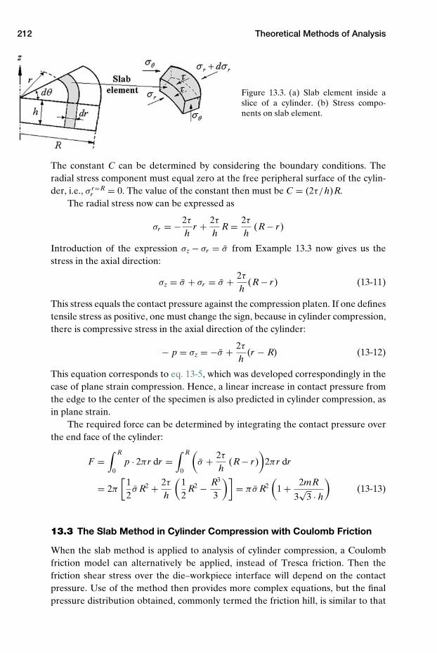
212 Theoretical Methods of Analysis
Figure 13.3. (a) Slab element inside aslice of a cylinder. (b) Stress compo-nents on slab element.
The constant C can be determined by considering the boundary conditions. Theradial stress component must equal zero at the free peripheral surface of the cylin-der, i.e., σ r=R
r = 0. The value of the constant then must be C = (2τ/h)R.The radial stress now can be expressed as
σr = −2τ
hr + 2τ
hR = 2τ
h(R − r)
Introduction of the expression σz − σr = σ from Example 13.3 now gives us thestress in the axial direction:
σz = σ + σr = σ + 2τ
h(R − r) (13-11)
This stress equals the contact pressure against the compression platen. If one definestensile stress as positive, one must change the sign, because in cylinder compression,there is compressive stress in the axial direction of the cylinder:
− p = σz = −σ + 2τ
h(r − R) (13-12)
This equation corresponds to eq. 13-5, which was developed correspondingly in thecase of plane strain compression. Hence, a linear increase in contact pressure fromthe edge to the center of the specimen is also predicted in cylinder compression, asin plane strain.
The required force can be determined by integrating the contact pressure overthe end face of the cylinder:
F =∫ R
0p · 2πr dr =
∫ R
0
(σ + 2τ
h(R − r)
)2πr dr
= 2π
[12σ R2 + 2τ
h
(12
R2 − R3
3
)]= πσ R2
(1 + 2mR
3√
3 · h
)(13-13)
13.3 The Slab Method in Cylinder Compression with Coulomb Friction
When the slab method is applied to analysis of cylinder compression, a Coulombfriction model can alternatively be applied, instead of Tresca friction. Then thefriction shear stress over the die–workpiece interface will depend on the contactpressure. Use of the method then provides more complex equations, but the finalpressure distribution obtained, commonly termed the friction hill, is similar to that
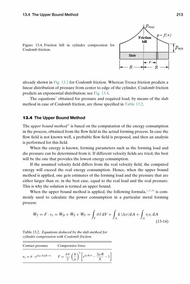
13.4 The Upper Bound Method 213
Figure 13.4. Friction hill in cylinder compression forCoulomb friction.
already shown in Fig. 13.2 for Coulomb friction. Whereas Tresca friction predicts alinear distribution of pressure from center to edge of the cylinder, Coulomb frictionpredicts an exponential distribution; see Fig. 13.4.
The equations7 obtained for pressure and required load, by means of the slabmethod in case of Coulomb friction, are those specified in Table 13.2.
13.4 The Upper Bound Method
The upper bound method 8 is based on the computation of the energy consumptionin the process, obtained from the flow field in the actual forming process. In case theflow field is not known well, a probable flow field is proposed, and then an analysisis performed for this field.
When the energy is known, forming parameters such as the forming load anddie pressure can be determined from it. If different velocity fields are tried, the bestwill be the one that provides the lowest energy consumption.
If the assumed velocity field differs from the real velocity field, the computedenergy will exceed the real energy consumption. Hence, when the upper boundmethod is applied, one gets estimates of the forming load and the pressure that areeither larger than or, in the best case, equal to the real load and the real pressure.This is why the solution is termed an upper bound.
When the upper bound method is applied, the following formula,1,9,10 is com-monly used to calculate the power consumption in a particular metal formingprocess:
WT = F · vs = WD + WS + WF =∫
Vσ ˙ε dV +
∫A
k |�v| dA +∫
Aτi vi dA
(13-14)
Table 13.2. Equations deduced by the slab method forcylinder compression with Coulomb friction
Contact pressure Compressive force
σz = σ · e(2µ/h)(R−r) F = πσ
2
(hµ
)2 [e2µR/h − 2µR
h− 1
]
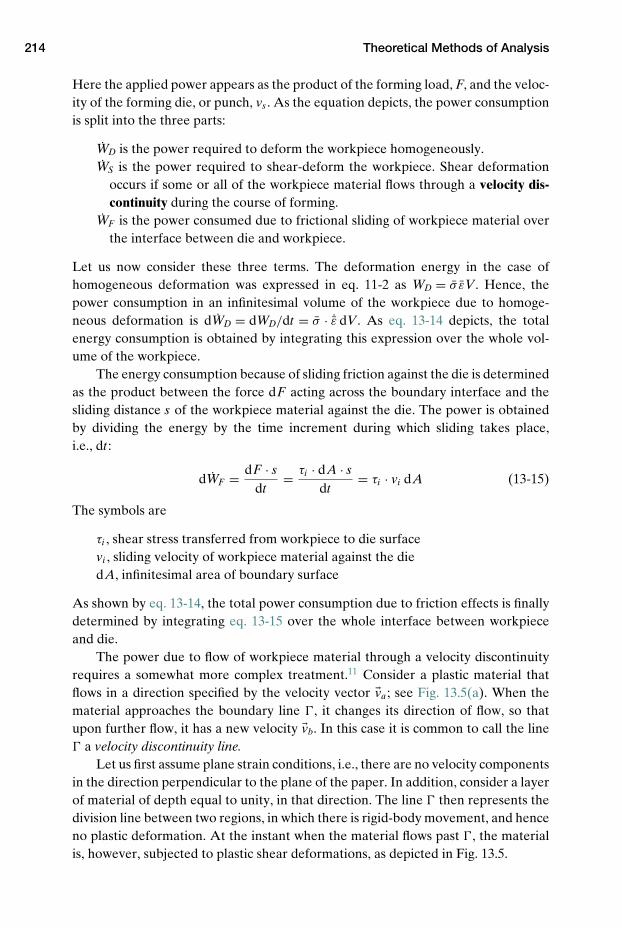
214 Theoretical Methods of Analysis
Here the applied power appears as the product of the forming load, F, and the veloc-ity of the forming die, or punch, vs . As the equation depicts, the power consumptionis split into the three parts:
WD is the power required to deform the workpiece homogeneously.WS is the power required to shear-deform the workpiece. Shear deformation
occurs if some or all of the workpiece material flows through a velocity dis-continuity during the course of forming.
WF is the power consumed due to frictional sliding of workpiece material overthe interface between die and workpiece.
Let us now consider these three terms. The deformation energy in the case ofhomogeneous deformation was expressed in eq. 11-2 as WD = σ εV. Hence, thepower consumption in an infinitesimal volume of the workpiece due to homoge-neous deformation is dWD = dWD/dt = σ · ˙ε dV. As eq. 13-14 depicts, the totalenergy consumption is obtained by integrating this expression over the whole vol-ume of the workpiece.
The energy consumption because of sliding friction against the die is determinedas the product between the force dF acting across the boundary interface and thesliding distance s of the workpiece material against the die. The power is obtainedby dividing the energy by the time increment during which sliding takes place,i.e., dt :
dWF = dF · sdt
= τi · dA · sdt
= τi · vi dA (13-15)
The symbols are
τi , shear stress transferred from workpiece to die surfacevi , sliding velocity of workpiece material against the diedA, infinitesimal area of boundary surface
As shown by eq. 13-14, the total power consumption due to friction effects is finallydetermined by integrating eq. 13-15 over the whole interface between workpieceand die.
The power due to flow of workpiece material through a velocity discontinuityrequires a somewhat more complex treatment.11 Consider a plastic material thatflows in a direction specified by the velocity vector va ; see Fig. 13.5(a). When thematerial approaches the boundary line �, it changes its direction of flow, so thatupon further flow, it has a new velocity vb. In this case it is common to call the line� a velocity discontinuity line.
Let us first assume plane strain conditions, i.e., there are no velocity componentsin the direction perpendicular to the plane of the paper. In addition, consider a layerof material of depth equal to unity, in that direction. The line � then represents thedivision line between two regions, in which there is rigid-body movement, and henceno plastic deformation. At the instant when the material flows past �, the materialis, however, subjected to plastic shear deformations, as depicted in Fig. 13.5.
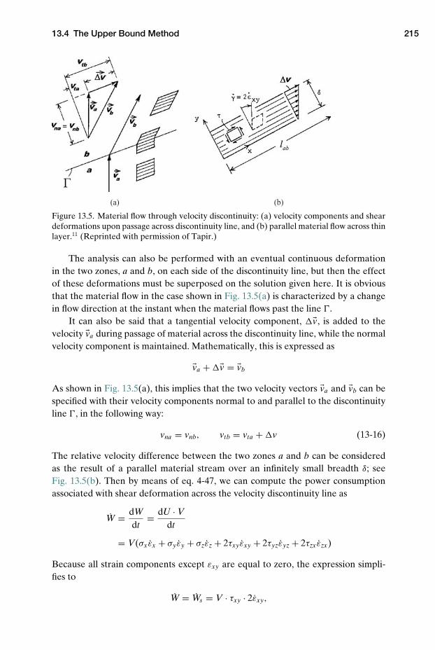
13.4 The Upper Bound Method 215
(a) (b)
Figure 13.5. Material flow through velocity discontinuity: (a) velocity components and sheardeformations upon passage across discontinuity line, and (b) parallel material flow across thinlayer.11 (Reprinted with permission of Tapir.)
The analysis can also be performed with an eventual continuous deformationin the two zones, a and b, on each side of the discontinuity line, but then the effectof these deformations must be superposed on the solution given here. It is obviousthat the material flow in the case shown in Fig. 13.5(a) is characterized by a changein flow direction at the instant when the material flows past the line �.
It can also be said that a tangential velocity component, � v, is added to thevelocity va during passage of material across the discontinuity line, while the normalvelocity component is maintained. Mathematically, this is expressed as
va + � v = vb
As shown in Fig. 13.5(a), this implies that the two velocity vectors va and vb can bespecified with their velocity components normal to and parallel to the discontinuityline �, in the following way:
vna = vnb, vtb = vta + �v (13-16)
The relative velocity difference between the two zones a and b can be consideredas the result of a parallel material stream over an infinitely small breadth δ; seeFig. 13.5(b). Then by means of eq. 4-47, we can compute the power consumptionassociated with shear deformation across the velocity discontinuity line as
W = dWdt
= dU · Vdt
= V(σx εx + σyεy + σzεz + 2τxyεxy + 2τyzεyz + 2τzx εzx)
Because all strain components except εxy are equal to zero, the expression simpli-fies to
W = Ws = V · τxy · 2εxy,
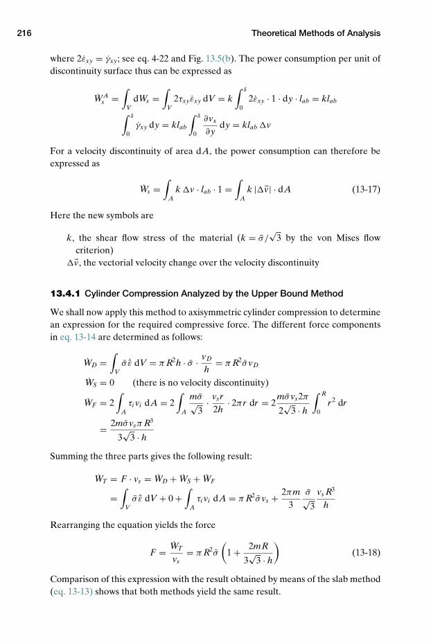
216 Theoretical Methods of Analysis
where 2εxy = γxy; see eq. 4-22 and Fig. 13.5(b). The power consumption per unit ofdiscontinuity surface thus can be expressed as
WAs =
∫V
dWs =∫
V2τxyεxy dV = k
∫ δ
02εxy · 1 · dy · lab = klab∫ δ
0γxy dy = klab
∫ δ
0
∂vx
∂ydy = klab �v
For a velocity discontinuity of area dA, the power consumption can therefore beexpressed as
Ws =∫
Ak �v · lab · 1 =
∫A
k |� v| · dA (13-17)
Here the new symbols are
k, the shear flow stress of the material (k = σ /√
3 by the von Mises flowcriterion)
� v, the vectorial velocity change over the velocity discontinuity
13.4.1 Cylinder Compression Analyzed by the Upper Bound Method
We shall now apply this method to axisymmetric cylinder compression to determinean expression for the required compressive force. The different force componentsin eq. 13-14 are determined as follows:
WD =∫
Vσ ˙ε dV = π R2h · σ · vD
h= π R2σvD
WS = 0 (there is no velocity discontinuity)
WF = 2∫
Aτi vi dA = 2
∫A
mσ√3
· vsr2h
· 2πr dr = 2mσvs2π
2√
3 · h
∫ R
0r2 dr
= 2mσvsπ R3
3√
3 · h
Summing the three parts gives the following result:
WT = F · vs = WD + WS + WF
=∫
Vσ ˙ε dV + 0 +
∫A
τi vi dA = π R2σvs + 2πm3
σ√3
vs R3
h
Rearranging the equation yields the force
F = WT
vs= π R2σ
(1 + 2mR
3√
3 · h
)(13-18)
Comparison of this expression with the result obtained by means of the slab method(eq. 13-13) shows that both methods yield the same result.
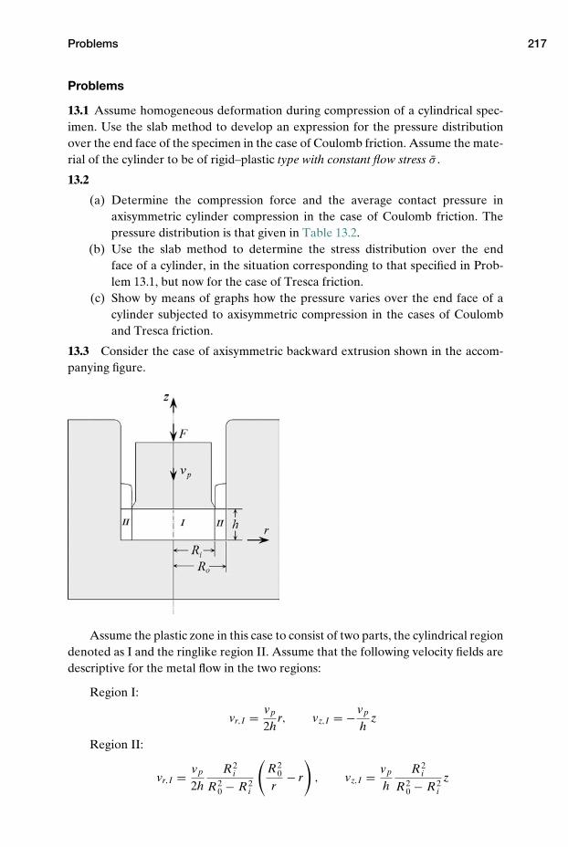
Problems 217
Problems
13.1 Assume homogeneous deformation during compression of a cylindrical spec-imen. Use the slab method to develop an expression for the pressure distributionover the end face of the specimen in the case of Coulomb friction. Assume the mate-rial of the cylinder to be of rigid–plastic type with constant flow stress σ .
13.2
(a) Determine the compression force and the average contact pressure inaxisymmetric cylinder compression in the case of Coulomb friction. Thepressure distribution is that given in Table 13.2.
(b) Use the slab method to determine the stress distribution over the endface of a cylinder, in the situation corresponding to that specified in Prob-lem 13.1, but now for the case of Tresca friction.
(c) Show by means of graphs how the pressure varies over the end face of acylinder subjected to axisymmetric compression in the cases of Coulomband Tresca friction.
13.3 Consider the case of axisymmetric backward extrusion shown in the accom-panying figure.
Assume the plastic zone in this case to consist of two parts, the cylindrical regiondenoted as I and the ringlike region II. Assume that the following velocity fields aredescriptive for the metal flow in the two regions:
Region I:
vr,I = vp
2hr, vz,I = −vp
hz
Region II:
vr,I = vp
2hR2
i
R20 − R2
i
(R2
0
r− r
), vz,I = vp
hR2
i
R20 − R2
i
z
218 Theoretical Methods of Analysis
Use the upper bound method to find a formula for the required punch load in thiscase.
NOTES
1. Altan, T., Oh, S.-I, and Gegel, H. L.: “Metal Forming: Fundamentals and Applications,”ASM Int. 1983, pp. 131–142.
2. Hosford, W. H., and Caddell, R. M.: “Metal Forming, Mechanics And Metallurgy,” 3rded., Cambridge Univ. Press, 2007.
3. Siebel, E.: “Forces and material flow in plastic deformation” (in German), Stahl u. Eisen,Vol. 45, 1925, pp. 1563–1566.
4. von Karman, T.: “Contribution to the theory of rolling” (in German), Z. AngewandteMathematik u. Mechanik, Vol. 5, 1925, pp. 139–141.
5. Sachs, G.: “On the theory of the tension test” (in German), Z. Angewandte Mathematiku. Mechanik, Vol. 7, 1927, pp. 235–236.
6. Siebel, E., and Pomp, A.: “On the further development of the compression test” (inGerman), Mitt. Kaiser-Wilhelm Inst. Eisenforschung, Vol. 10, 1928, pp. 55–62.
7. Dieter, G. E.: “Mechanical Metallurgy,” McGraw-Hill, 1989.8. Prager, W., and Hodge, P. G.: “Theory of Perfectly Plastic Solids,” Wiley, New York,
1941.9. Steck, E.: “Load determination in metal forming by use of the upper bound theorem”
(in German), Werkstattstechnik, Vol. 57, 1967, pp. 273–279.10. Avitzur, B: “Metal Forming: Processes and Analysis,” McGraw-Hill, New York, 1968.11. Hellan, K.: “Theory of Plasticity,” Tapir, 1972, pp. 82–84 (in Norwegian).
REFERENCES
Altan, T., Oh, S.-I., and Gegel, H. L.: “Metal Forming, Fundamentals and Applications,”ASM Int. 1983, pp. 131–142.
Dieter, G. E.: “Mechanical Metallurgy,” McGraw-Hill, 1989.Lange, K.: “Handbook of Metal Forming,” McGraw-Hill, 1985.
14 Finite Element Analysis
Lately, the most important advancement in metal forming analysis has been thedevelopment and application of finite element analysis (FEA), i.e., use of the com-puterized finite element method (FEM). Recent progress in FEA, together withincreasingly powerful computers, has permitted increased use of such numericalmodeling. Hence, today it is possible to FEM-simulate the metal forming processesat various design stages.
When a FEM model has been made for a particular forming application,the load requirement, velocity, strain rate, strain and stress fields, etc., can eas-ily be obtained for the considered process. Therefore, the current trend is towardincreased application of FEA for process simulation and optimization. For practicalapplications, the modeling techniques must, of course, describe experimental obser-vations quantitatively with sufficient accuracy.
After an introduction to modeling techniques in general in metal forming, thischapter will focus on the application of FEM modeling as a practical tool to investi-gate the process conditions in forming operations. An overview of some commonlyapplied FEM codes will be given. Afterwards, it will be shown how the two- andthree-dimensional versions of the DEFORMTM FEM program can be used to FEM-model metal forming.
Some examples will be presented where the DEFORM FEM code is used fordeformation analysis in practical metal forming cases like plane strain compressionand cylinder compression. Finally, a case will be presented where the complex con-ditions in extrusion welding are investigated by means of FEA. There is work beingdone to create corresponding models using QFORM. The DEFORM and QFORMmodels will be available at www.cambridge.org/valberg.
14.1 Modeling Techniques in Metal Forming
There are three primary goals in performing an engineering analysis of metal form-ing. First, the analysis aims at reduced efforts of trial and error in tool and pro-cess design. Second, the analysis approach is useful in order to design the desiredpart for ease of manufacture. Finally, there may be problems in the process that
219

220 Finite Element Analysis
need to be solved. The analysis approach commonly lowers tooling and equip-ment costs, provides improved tooling modifications, and helps in understanding theprocess. It may lead to faster production of quality products at minimum cost,including reduced material waste and shortened lead times.
In early metal forming technology, the design of a forming process, and predic-tions of material flow and forming loads, depended mainly upon the experience andthe intuition of the metal former. Sometimes this led to costly trial-and-error exper-imentation in the design of new forming operations. To be able to reach the goalfaster and with less effort, and to increase the understanding of the mechanics ofmetal forming operations, modeling techniques have been developed over the years.
Modeling techniques1 can be said to cover all methods used to determine processparameters without conducting the actual forming process itself. They are used torefine existing process techniques or to investigate new techniques. Important pro-cess parameters in metal forming are, for example, force–stroke diagrams, energyrequirements, deformation characteristics and material flow, and the distribution ofstress, strain, and strain rate inside the deforming body. Modeling techniques arecommonly either physical or numerical techniques.
Physical modeling techniques involve the use of experiments applying modelmaterials or tailored materials or experiments on special metal forming processes.Physical modeling includes experiments on special test specimens used in metalforming; see Ch. 3. Material flow and strain distribution studies can, for instance, asdescribed in Ch. 12, be conducted over a cross section of a test workpiece in forming,for instance, by placing patterns on its surface or at preferred cross sections.
Numerical modeling techniques, on the other hand, analyze a process numeri-cally with the help of mathematics. Numerical computation results are commonlyvalidated by comparison with measured data, such as the shape change or therequired forming load. Physical and numerical modeling of metal forming processeshelp understand the processes better, for optimization purposes.
Many numerical methods have been developed to analyze metal forming. Clas-sical methods like the slab, the upper and the lower bound, and the slip-line fieldmethods (see Ch. 13), are all numerical methods. They are still useful for predict-ing approximate optimum process variables, such as forming loads, overall geome-try changes of the workpiece, and qualitative modes of material flow. Hence, thesemethods still provide useful information and understanding about the mechanics ofmetal forming.
14.2 FEM Analysis
The first effort to develop the FEM date back to work done in 1941–1942.2 Themethod was further developed in the following decades and was provided with amathematical foundation in 1973.3 FEM is a numerical technique for finding approx-imate solutions of partial differential equations and integral equations. The methodwas first applied in structural mechanics and is usually based on an energy princi-ple such as that of virtual work or minimum total potential energy. FEA is todaygenerally used for prediction of stresses and displacements in mechanical objects
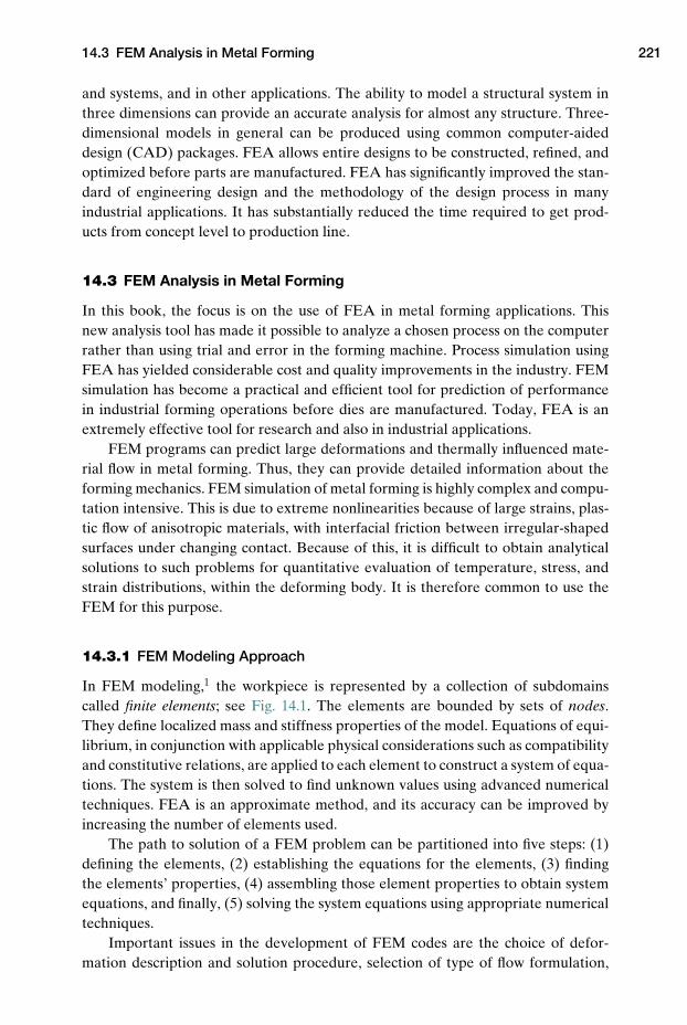
14.3 FEM Analysis in Metal Forming 221
and systems, and in other applications. The ability to model a structural system inthree dimensions can provide an accurate analysis for almost any structure. Three-dimensional models in general can be produced using common computer-aideddesign (CAD) packages. FEA allows entire designs to be constructed, refined, andoptimized before parts are manufactured. FEA has significantly improved the stan-dard of engineering design and the methodology of the design process in manyindustrial applications. It has substantially reduced the time required to get prod-ucts from concept level to production line.
14.3 FEM Analysis in Metal Forming
In this book, the focus is on the use of FEA in metal forming applications. Thisnew analysis tool has made it possible to analyze a chosen process on the computerrather than using trial and error in the forming machine. Process simulation usingFEA has yielded considerable cost and quality improvements in the industry. FEMsimulation has become a practical and efficient tool for prediction of performancein industrial forming operations before dies are manufactured. Today, FEA is anextremely effective tool for research and also in industrial applications.
FEM programs can predict large deformations and thermally influenced mate-rial flow in metal forming. Thus, they can provide detailed information about theforming mechanics. FEM simulation of metal forming is highly complex and compu-tation intensive. This is due to extreme nonlinearities because of large strains, plas-tic flow of anisotropic materials, with interfacial friction between irregular-shapedsurfaces under changing contact. Because of this, it is difficult to obtain analyticalsolutions to such problems for quantitative evaluation of temperature, stress, andstrain distributions, within the deforming body. It is therefore common to use theFEM for this purpose.
14.3.1 FEM Modeling Approach
In FEM modeling,1 the workpiece is represented by a collection of subdomainscalled finite elements; see Fig. 14.1. The elements are bounded by sets of nodes.They define localized mass and stiffness properties of the model. Equations of equi-librium, in conjunction with applicable physical considerations such as compatibilityand constitutive relations, are applied to each element to construct a system of equa-tions. The system is then solved to find unknown values using advanced numericaltechniques. FEA is an approximate method, and its accuracy can be improved byincreasing the number of elements used.
The path to solution of a FEM problem can be partitioned into five steps: (1)defining the elements, (2) establishing the equations for the elements, (3) findingthe elements’ properties, (4) assembling those element properties to obtain systemequations, and finally, (5) solving the system equations using appropriate numericaltechniques.
Important issues in the development of FEM codes are the choice of defor-mation description and solution procedure, selection of type of flow formulation,
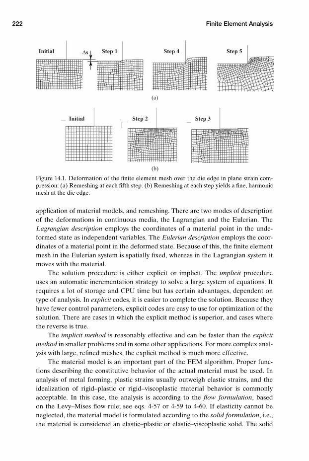
222 Finite Element Analysis
Step 2 Step 3Initial
Step 1∆s Step 4 Step 5Initial
(a)
(b)
Figure 14.1. Deformation of the finite element mesh over the die edge in plane strain com-pression: (a) Remeshing at each fifth step. (b) Remeshing at each step yields a fine, harmonicmesh at the die edge.
application of material models, and remeshing. There are two modes of descriptionof the deformations in continuous media, the Lagrangian and the Eulerian. TheLagrangian description employs the coordinates of a material point in the unde-formed state as independent variables. The Eulerian description employs the coor-dinates of a material point in the deformed state. Because of this, the finite elementmesh in the Eulerian system is spatially fixed, whereas in the Lagrangian system itmoves with the material.
The solution procedure is either explicit or implicit. The implicit procedureuses an automatic incrementation strategy to solve a large system of equations. Itrequires a lot of storage and CPU time but has certain advantages, dependent ontype of analysis. In explicit codes, it is easier to complete the solution. Because theyhave fewer control parameters, explicit codes are easy to use for optimization of thesolution. There are cases in which the explicit method is superior, and cases wherethe reverse is true.
The implicit method is reasonably effective and can be faster than the explicitmethod in smaller problems and in some other applications. For more complex anal-ysis with large, refined meshes, the explicit method is much more effective.
The material model is an important part of the FEM algorithm. Proper func-tions describing the constitutive behavior of the actual material must be used. Inanalysis of metal forming, plastic strains usually outweigh elastic strains, and theidealization of rigid–plastic or rigid–viscoplastic material behavior is commonlyacceptable. In this case, the analysis is according to the flow formulation, basedon the Levy–Mises flow rule; see eqs. 4-57 or 4-59 to 4-60. If elasticity cannot beneglected, the material model is formulated according to the solid formulation, i.e.,the material is considered an elastic–plastic or elastic–viscoplastic solid. The solid
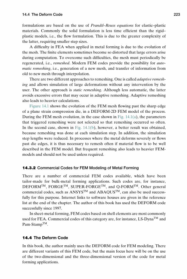
14.4 The Deform Code 223
formulations are based on the use of Prandtl–Reuss equations for elastic–plasticmaterials. Commonly the solid formulation is less time efficient than the rigid–plastic models, i.e., the flow formulation. This is due to the greater complexity ofthe latter, requiring smaller step sizes.
A difficulty in FEA when applied in metal forming is due to the evolution ofthe mesh. The finite elements sometimes become so distorted that large errors ariseduring computation. To overcome such difficulties, the mesh must periodically beregenerated, i.e., remeshed. Modern FEM codes provide the possibility for auto-matic remeshing, i.e., generation of a new mesh, and transfer of information fromold to new mesh through interpolation.
There are two different approaches to remeshing. One is called adaptive remesh-ing and allows simulation of large deformations without any intervention by theuser. The other approach is static remeshing. Although less automatic, the latteravoids excessive errors that may occur in adaptive remeshing. Adaptive remeshingalso leads to heavier calculations.
Figure 14.1 shows the evolution of the FEM mesh flowing past the sharp edgeof a plane strain compression die, in a DEFORM-2D FEM model of the process.During the FEM mesh evolution, in the case shown in Fig. 14.1(a), the parametersthat triggered remeshing were not selected so that remeshing occurred so often.In the second case, shown in Fig. 14.1(b), however, a better result was obtained,because remeshing was done at each simulation step. In addition, the simulationstep lengths were reduced. In processes where the metal deforms severely or flowspast die edges, it is thus necessary to remesh often if material flow is to be welldescribed in the FEM model. But frequent remeshing also leads to heavier FEM-models and should not be used unless required.
14.3.2 Commercial Codes for FEM Modeling of Metal Forming
There are a number of commercial FEM codes available, which have beentailor-made for bulk-metal forming applications. Such codes are, for instance,DEFORMTM, FORGETM, SUPER-FORGETM, and Q-FORMTM. Other generalcommercial codes, such as ANSYSTM and ABAQUSTM, can also be used success-fully for this purpose. Internet links to software houses are given in the referencelist at the end of the chapter. The author of this book has used the DEFORM codesuccessfully since 1997.
In sheet-metal forming, FEM codes based on shell elements are most commonlyused for FEA. Commercial codes of this category are, for instance, LS-DynaTM andPam-StampTM.
14.4 The Deform Code
In this book, the author mainly uses the DEFORM code for FEM modeling. Thereare different variants of this FEM code, but the main focus here will be on the useof the two-dimensional and the three-dimensional version of the code for metalforming applications.
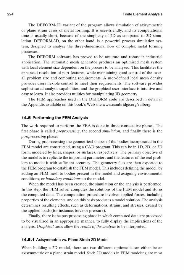
224 Finite Element Analysis
The DEFORM-2D variant of the program allows simulation of axisymmetricor plane strain cases of metal forming. It is user-friendly, and its computationaltime is usually short, because of the simplicity of 2D as compared to 3D simu-lation. DEFORM-3D, on the other hand, is a powerful process simulation sys-tem, designed to analyze the three-dimensional flow of complex metal formingprocesses.
The DEFORM software has proved to be accurate and robust in industrialapplication. The automatic mesh generator produces an optimized mesh systemwith local element size dependent on the process to be analyzed. This facilitates theenhanced resolution of part features, while maintaining good control of the over-all problem size and computing requirements. A user-defined local mesh densityprovides users flexible control to meet their requirements. The software providessophisticated analysis capabilities, and the graphical user interface is intuitive andeasy to learn. It also provides utilities for manipulating 3D geometry.
The FEM approaches used in the DEFORM code are described in detail inthe Appendix available on this book’s Web site www.cambridge.org/valberg.
14.5 Performing the FEM Analysis
The work required to perform the FEA is done in three consecutive phases. Thefirst phase is called preprocessing, the second simulation, and finally there is thepostprocessing phase.
During preprocessing the geometrical shapes of the bodies incorporated in theFEM model are constructed, using a CAD program. This can be in 1D, 2D, or 3Dform, modeled by lines, shapes, or surfaces, respectively. The primary objective ofthe model is to replicate the important parameters and the features of the real prob-lem to model it with sufficient accuracy. The geometry files are then exported tothe FEM program to establish the FEM model. This includes defining the model, byadding an FEM mesh to bodies present in the model and assigning environmentalconditions, or boundary conditions, to the model.
When the model has been created, the simulation or the analysis is performed.In this step, the FEM solver computes the solutions of the FEM model and storesthe computed data. The computation procedure involves applied forces, includingproperties of the elements, and on this basis produces a model solution. The analysisdetermines resulting effects, such as deformations, strains, and stresses, caused bythe applied loads (for instance, force or pressure).
Finally, there is the postprocessing phase in which computed data are processedto be visualized in an appropriate manner, to fully display the implications of theanalysis. Graphical tools allow the results of the analysis to be interpreted.
14.5.1 Axisymmetric vs. Plane Strain 2D Model
When building a 2D model, there are two different options: it can either be anaxisymmetric or a plane strain model. Such 2D models in FEM modeling are most
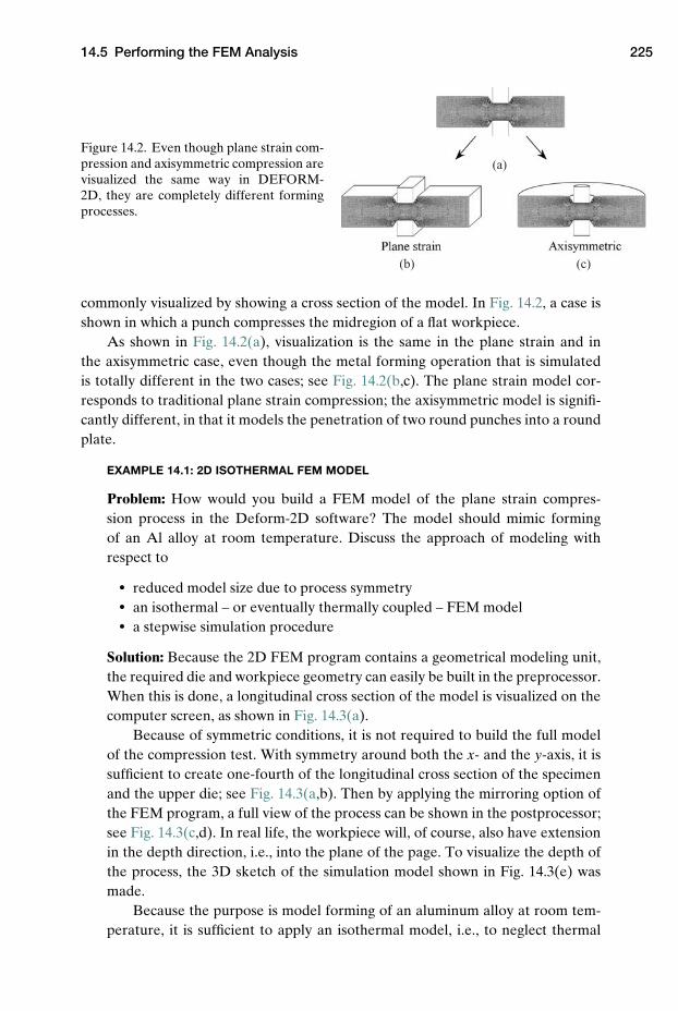
14.5 Performing the FEM Analysis 225
(a)
(b) (c)
Figure 14.2. Even though plane strain com-pression and axisymmetric compression arevisualized the same way in DEFORM-2D, they are completely different formingprocesses.
commonly visualized by showing a cross section of the model. In Fig. 14.2, a case isshown in which a punch compresses the midregion of a flat workpiece.
As shown in Fig. 14.2(a), visualization is the same in the plane strain and inthe axisymmetric case, even though the metal forming operation that is simulatedis totally different in the two cases; see Fig. 14.2(b,c). The plane strain model cor-responds to traditional plane strain compression; the axisymmetric model is signifi-cantly different, in that it models the penetration of two round punches into a roundplate.
EXAMPLE 14.1: 2D ISOTHERMAL FEM MODEL
Problem: How would you build a FEM model of the plane strain compres-sion process in the Deform-2D software? The model should mimic formingof an Al alloy at room temperature. Discuss the approach of modeling withrespect to
� reduced model size due to process symmetry� an isothermal – or eventually thermally coupled – FEM model� a stepwise simulation procedure
Solution: Because the 2D FEM program contains a geometrical modeling unit,the required die and workpiece geometry can easily be built in the preprocessor.When this is done, a longitudinal cross section of the model is visualized on thecomputer screen, as shown in Fig. 14.3(a).
Because of symmetric conditions, it is not required to build the full modelof the compression test. With symmetry around both the x- and the y-axis, it issufficient to create one-fourth of the longitudinal cross section of the specimenand the upper die; see Fig. 14.3(a,b). Then by applying the mirroring option ofthe FEM program, a full view of the process can be shown in the postprocessor;see Fig. 14.3(c,d). In real life, the workpiece will, of course, also have extensionin the depth direction, i.e., into the plane of the page. To visualize the depth ofthe process, the 3D sketch of the simulation model shown in Fig. 14.3(e) wasmade.
Because the purpose is model forming of an aluminum alloy at room tem-perature, it is sufficient to apply an isothermal model, i.e., to neglect thermal
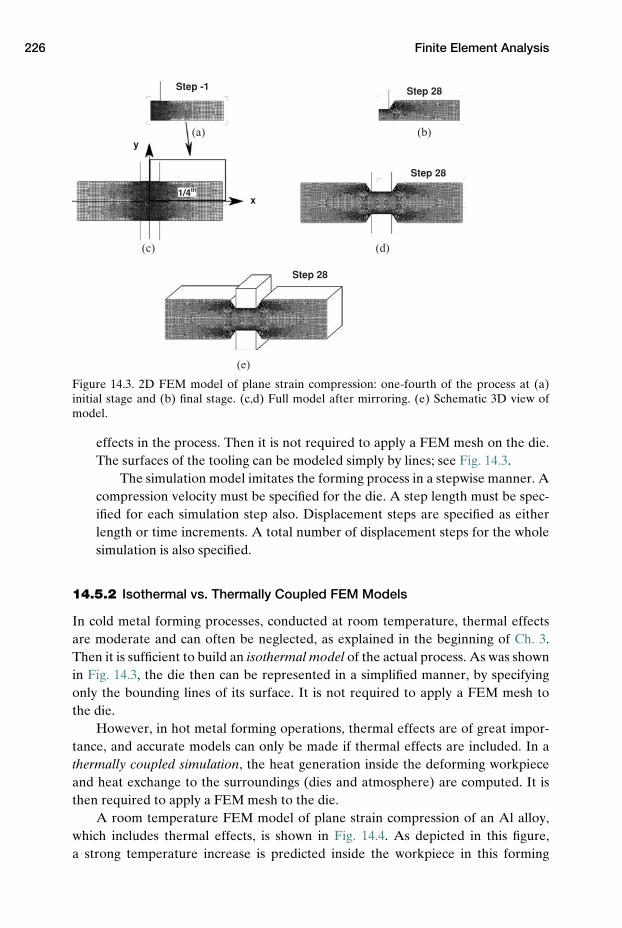
226 Finite Element Analysis
(a) (b)
(d)(c)
(e)
Step -1 Step 28
Step 28
Step 28
x
y
1/4th
Figure 14.3. 2D FEM model of plane strain compression: one-fourth of the process at (a)initial stage and (b) final stage. (c,d) Full model after mirroring. (e) Schematic 3D view ofmodel.
effects in the process. Then it is not required to apply a FEM mesh on the die.The surfaces of the tooling can be modeled simply by lines; see Fig. 14.3.
The simulation model imitates the forming process in a stepwise manner. Acompression velocity must be specified for the die. A step length must be spec-ified for each simulation step also. Displacement steps are specified as eitherlength or time increments. A total number of displacement steps for the wholesimulation is also specified.
14.5.2 Isothermal vs. Thermally Coupled FEM Models
In cold metal forming processes, conducted at room temperature, thermal effectsare moderate and can often be neglected, as explained in the beginning of Ch. 3.Then it is sufficient to build an isothermal model of the actual process. As was shownin Fig. 14.3, the die then can be represented in a simplified manner, by specifyingonly the bounding lines of its surface. It is not required to apply a FEM mesh tothe die.
However, in hot metal forming operations, thermal effects are of great impor-tance, and accurate models can only be made if thermal effects are included. In athermally coupled simulation, the heat generation inside the deforming workpieceand heat exchange to the surroundings (dies and atmosphere) are computed. It isthen required to apply a FEM mesh to the die.
A room temperature FEM model of plane strain compression of an Al alloy,which includes thermal effects, is shown in Fig. 14.4. As depicted in this figure,a strong temperature increase is predicted inside the workpiece in this forming
14.5 Performing the FEM Analysis 227
operation. But because the flow stress is not much affected by heating of theworkpiece material up to a temperature of (say) 100◦C, temperature effects on loadsand stresses are modest and can be neglected without much error.
However, if an accurate analysis is required, thermal effects should also beincluded in cold-forming applications. This is especially important if the formingis rapid and if there are large deformations in the specimen, because there will thenbe larger local temperature rise.
In plane strain compression of an aluminum alloy, as Fig. 14.4 depicts, heateffects are predicted to be largest in the shear cross formed in the material, insidethe compression gap, as well as in the material flowing over the sharp edge of thedie. Heat transfer to the die, however, is predicted to be rather modest.
One should be aware that industrial forming is usually done repeatedly, so thetooling heats up gradually, from room temperature in the beginning of the process,to a stable elevated temperature after a number of pieces have been shaped.
14.5.3 Material Behavior
In many metal forming applications, one can consider the die as rigid and the work-piece material as rigid–plastic, and this approximation will suffice to get models thatmimic the real processes with good accuracy. For instance, the FEM model used tomodel plane strain compression and to compute thermal conditions, in connectionwith simulation results shown in Fig. 14.4, was based on this material description.But in other applications, it may be required to apply other material descriptions.The DEFORM software has, for example, the capability of choosing different mate-rial behavior – rigid, plastic, elastic, elastic–plastic, or porous.
In case of forming sheet metal by bending, the workpiece will be subjected toelastic springback when the bending load is released, as shown in Fig. 24.4(a). Thespringback is caused by elastic stresses present in the thin elastically bent midlayerof the sheet. These elastic stresses can be said to counteract the bending process, andthey cause the specimen to bend back when the load is removed. Hence to model thephenomenon of springback, it is required to describe the full elastic–plastic behaviorof the bending specimen. The application of this type of material description is dealtwith in more depth in Ch. 25 available at www.cambridge.org/valberg.
14.5.4 Material Models
To be able to perform a simulation, it is necessary to specify to the FEM programthe flow curve of the workpiece material being used. Different material models weredealt with in the treatment in Ch. 8. FEM codes have options by which one canspecify, in a simple manner, a particular material model, as, for instance, by choosinga power-law material and then typing in the actual K and n values for the selectedmaterial.
If the workpiece material is characterized by flow stress data that do not agreewell with common applied material models, there is commonly the possibility to
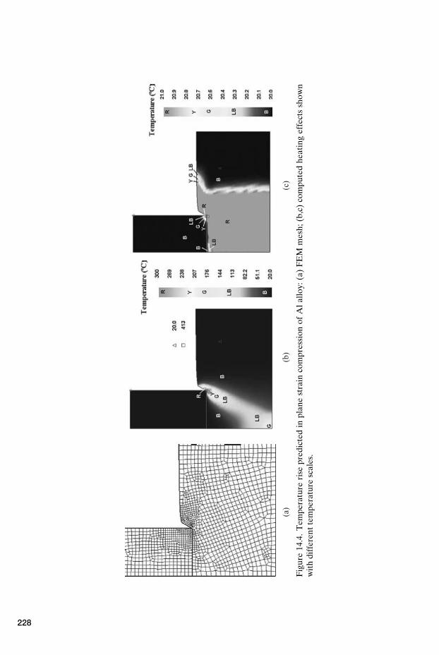
(a)
(b)
(c)
Fig
ure
14.4
.T
empe
ratu
reri
sepr
edic
ted
inpl
ane
stra
inco
mpr
essi
onof
Ala
lloy:
(a)
FE
Mm
esh;
(b,c
)co
mpu
ted
heat
ing
effe
cts
show
nw
ith
diff
eren
ttem
pera
ture
scal
es.
228
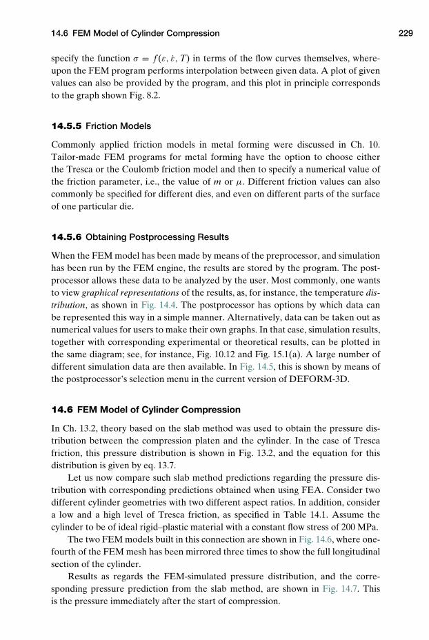
14.6 FEM Model of Cylinder Compression 229
specify the function σ = f (ε, ε, T) in terms of the flow curves themselves, where-upon the FEM program performs interpolation between given data. A plot of givenvalues can also be provided by the program, and this plot in principle correspondsto the graph shown Fig. 8.2.
14.5.5 Friction Models
Commonly applied friction models in metal forming were discussed in Ch. 10.Tailor-made FEM programs for metal forming have the option to choose eitherthe Tresca or the Coulomb friction model and then to specify a numerical value ofthe friction parameter, i.e., the value of m or µ. Different friction values can alsocommonly be specified for different dies, and even on different parts of the surfaceof one particular die.
14.5.6 Obtaining Postprocessing Results
When the FEM model has been made by means of the preprocessor, and simulationhas been run by the FEM engine, the results are stored by the program. The post-processor allows these data to be analyzed by the user. Most commonly, one wantsto view graphical representations of the results, as, for instance, the temperature dis-tribution, as shown in Fig. 14.4. The postprocessor has options by which data canbe represented this way in a simple manner. Alternatively, data can be taken out asnumerical values for users to make their own graphs. In that case, simulation results,together with corresponding experimental or theoretical results, can be plotted inthe same diagram; see, for instance, Fig. 10.12 and Fig. 15.1(a). A large number ofdifferent simulation data are then available. In Fig. 14.5, this is shown by means ofthe postprocessor’s selection menu in the current version of DEFORM-3D.
14.6 FEM Model of Cylinder Compression
In Ch. 13.2, theory based on the slab method was used to obtain the pressure dis-tribution between the compression platen and the cylinder. In the case of Trescafriction, this pressure distribution is shown in Fig. 13.2, and the equation for thisdistribution is given by eq. 13.7.
Let us now compare such slab method predictions regarding the pressure dis-tribution with corresponding predictions obtained when using FEA. Consider twodifferent cylinder geometries with two different aspect ratios. In addition, considera low and a high level of Tresca friction, as specified in Table 14.1. Assume thecylinder to be of ideal rigid–plastic material with a constant flow stress of 200 MPa.
The two FEM models built in this connection are shown in Fig. 14.6, where one-fourth of the FEM mesh has been mirrored three times to show the full longitudinalsection of the cylinder.
Results as regards the FEM-simulated pressure distribution, and the corre-sponding pressure prediction from the slab method, are shown in Fig. 14.7. Thisis the pressure immediately after the start of compression.
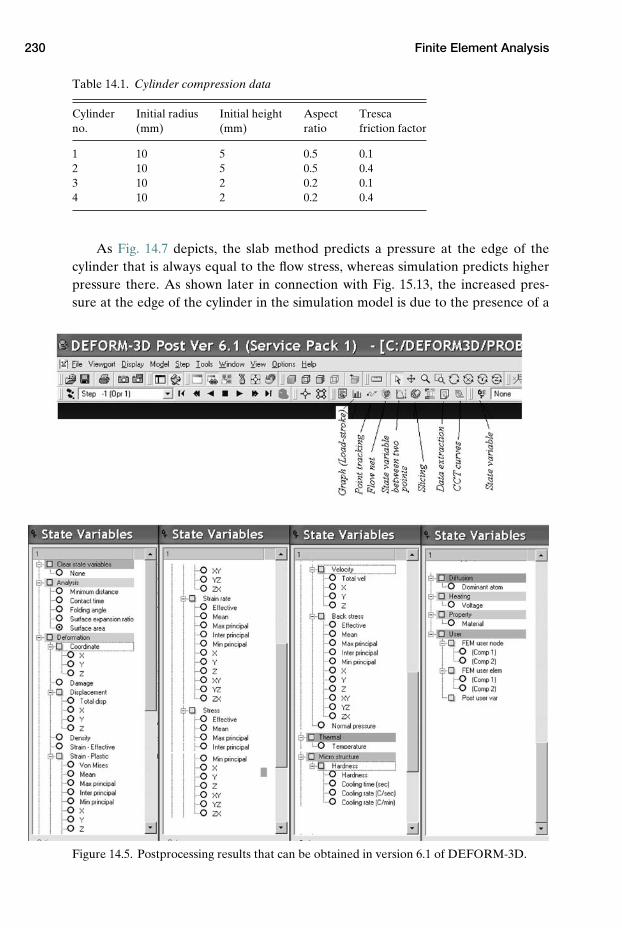
230 Finite Element Analysis
Table 14.1. Cylinder compression data
Cylinder Initial radius Initial height Aspect Trescano. (mm) (mm) ratio friction factor
1 10 5 0.5 0.12 10 5 0.5 0.43 10 2 0.2 0.14 10 2 0.2 0.4
As Fig. 14.7 depicts, the slab method predicts a pressure at the edge of thecylinder that is always equal to the flow stress, whereas simulation predicts higherpressure there. As shown later in connection with Fig. 15.13, the increased pres-sure at the edge of the cylinder in the simulation model is due to the presence of a
Figure 14.5. Postprocessing results that can be obtained in version 6.1 of DEFORM-3D.
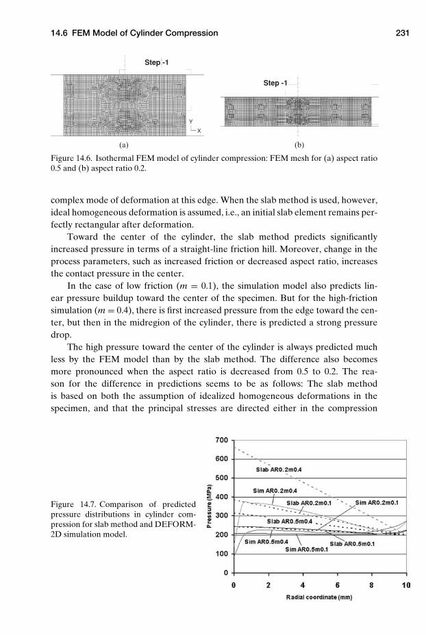
14.6 FEM Model of Cylinder Compression 231
Step -1
Step -1
X
Y
(a) (b)
Figure 14.6. Isothermal FEM model of cylinder compression: FEM mesh for (a) aspect ratio0.5 and (b) aspect ratio 0.2.
complex mode of deformation at this edge. When the slab method is used, however,ideal homogeneous deformation is assumed, i.e., an initial slab element remains per-fectly rectangular after deformation.
Toward the center of the cylinder, the slab method predicts significantlyincreased pressure in terms of a straight-line friction hill. Moreover, change in theprocess parameters, such as increased friction or decreased aspect ratio, increasesthe contact pressure in the center.
In the case of low friction (m = 0.1), the simulation model also predicts lin-ear pressure buildup toward the center of the specimen. But for the high-frictionsimulation (m = 0.4), there is first increased pressure from the edge toward the cen-ter, but then in the midregion of the cylinder, there is predicted a strong pressuredrop.
The high pressure toward the center of the cylinder is always predicted muchless by the FEM model than by the slab method. The difference also becomesmore pronounced when the aspect ratio is decreased from 0.5 to 0.2. The rea-son for the difference in predictions seems to be as follows: The slab methodis based on both the assumption of idealized homogeneous deformations in thespecimen, and that the principal stresses are directed either in the compression
Figure 14.7. Comparison of predictedpressure distributions in cylinder com-pression for slab method and DEFORM-2D simulation model.
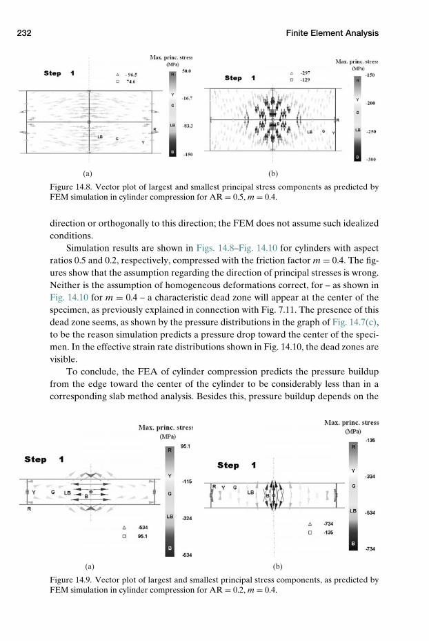
232 Finite Element Analysis
(a) (b)
Figure 14.8. Vector plot of largest and smallest principal stress components as predicted byFEM simulation in cylinder compression for AR = 0.5, m = 0.4.
direction or orthogonally to this direction; the FEM does not assume such idealizedconditions.
Simulation results are shown in Figs. 14.8–Fig. 14.10 for cylinders with aspectratios 0.5 and 0.2, respectively, compressed with the friction factor m = 0.4. The fig-ures show that the assumption regarding the direction of principal stresses is wrong.Neither is the assumption of homogeneous deformations correct, for – as shown inFig. 14.10 for m = 0.4 – a characteristic dead zone will appear at the center of thespecimen, as previously explained in connection with Fig. 7.11. The presence of thisdead zone seems, as shown by the pressure distributions in the graph of Fig. 14.7(c),to be the reason simulation predicts a pressure drop toward the center of the speci-men. In the effective strain rate distributions shown in Fig. 14.10, the dead zones arevisible.
To conclude, the FEA of cylinder compression predicts the pressure buildupfrom the edge toward the center of the cylinder to be considerably less than in acorresponding slab method analysis. Besides this, pressure buildup depends on the
(a) (b)
Figure 14.9. Vector plot of largest and smallest principal stress components, as predicted byFEM simulation in cylinder compression for AR = 0.2, m = 0.4.
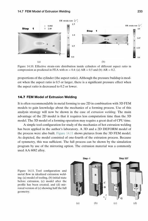
14.7 FEM Model of Extrusion Welding 233
(b)(a)
Figure 14.10. Effective strain-rate distribution inside cylinders of different aspect ratio incompression as predicted in FEA with m = 0.4: (a) AR = 0.5 and (b) AR = 0.2.
proportions of the cylinder (the aspect ratio). Although the pressure buildup is mod-est when the aspect ratio is 0.5 or larger, there is a significant pressure effect whenthe aspect ratio is decreased to 0.2 or lower.
14.7 FEM Model of Extrusion Welding
It is often recommendable in metal forming to use 2D in combination with 3D FEMmodels to gain knowledge about the mechanics of a forming process. Use of thisanalysis strategy will now be shown in the case of extrusion welding. The mainadvantage of the 2D model is that it requires less computation time than the 3Dmodel. The 3D model of a forming operation may require a great deal of CPU time.
A simple tool configuration for study of the mechanics of hot extrusion weldinghas been applied in the author’s laboratory. A 3D and a 2D DEFORM model ofthe process were also built. Figure 14.11 shows pictures from the 3D FEM model.As depicted, the model consisted of one-fourth of the extrusion process. Becauseof symmetry, this was sufficient. The full process can be shown by the simulationprogram by use of the mirroring option. The extrusion material was a commonlyused AA 6082 alloy.
(a) (b) (c) (d)
Figure 14.11. Tool configuration andmetal flow in idealized extrusion weld-ing: (a) model of tooling, (b) initial statebefore extrusion, (c) model after theprofile has been created, and (d) mir-rored version of (c) showing half the fullgeometry.
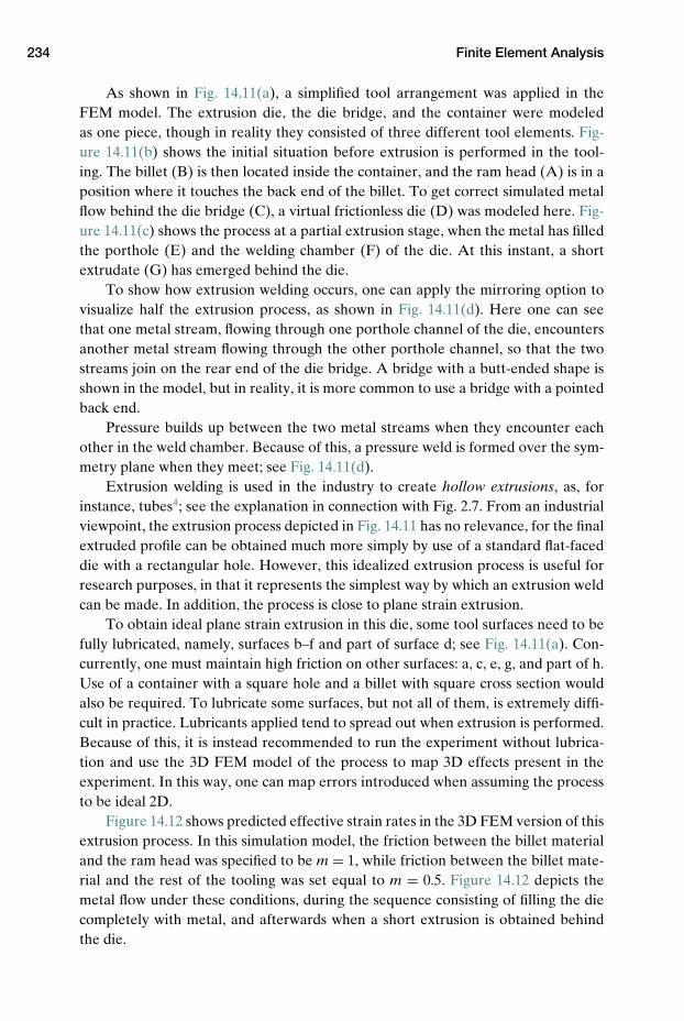
234 Finite Element Analysis
As shown in Fig. 14.11(a), a simplified tool arrangement was applied in theFEM model. The extrusion die, the die bridge, and the container were modeledas one piece, though in reality they consisted of three different tool elements. Fig-ure 14.11(b) shows the initial situation before extrusion is performed in the tool-ing. The billet (B) is then located inside the container, and the ram head (A) is in aposition where it touches the back end of the billet. To get correct simulated metalflow behind the die bridge (C), a virtual frictionless die (D) was modeled here. Fig-ure 14.11(c) shows the process at a partial extrusion stage, when the metal has filledthe porthole (E) and the welding chamber (F) of the die. At this instant, a shortextrudate (G) has emerged behind the die.
To show how extrusion welding occurs, one can apply the mirroring option tovisualize half the extrusion process, as shown in Fig. 14.11(d). Here one can seethat one metal stream, flowing through one porthole channel of the die, encountersanother metal stream flowing through the other porthole channel, so that the twostreams join on the rear end of the die bridge. A bridge with a butt-ended shape isshown in the model, but in reality, it is more common to use a bridge with a pointedback end.
Pressure builds up between the two metal streams when they encounter eachother in the weld chamber. Because of this, a pressure weld is formed over the sym-metry plane when they meet; see Fig. 14.11(d).
Extrusion welding is used in the industry to create hollow extrusions, as, forinstance, tubes4; see the explanation in connection with Fig. 2.7. From an industrialviewpoint, the extrusion process depicted in Fig. 14.11 has no relevance, for the finalextruded profile can be obtained much more simply by use of a standard flat-faceddie with a rectangular hole. However, this idealized extrusion process is useful forresearch purposes, in that it represents the simplest way by which an extrusion weldcan be made. In addition, the process is close to plane strain extrusion.
To obtain ideal plane strain extrusion in this die, some tool surfaces need to befully lubricated, namely, surfaces b–f and part of surface d; see Fig. 14.11(a). Con-currently, one must maintain high friction on other surfaces: a, c, e, g, and part of h.Use of a container with a square hole and a billet with square cross section wouldalso be required. To lubricate some surfaces, but not all of them, is extremely diffi-cult in practice. Lubricants applied tend to spread out when extrusion is performed.Because of this, it is instead recommended to run the experiment without lubrica-tion and use the 3D FEM model of the process to map 3D effects present in theexperiment. In this way, one can map errors introduced when assuming the processto be ideal 2D.
Figure 14.12 shows predicted effective strain rates in the 3D FEM version of thisextrusion process. In this simulation model, the friction between the billet materialand the ram head was specified to be m = 1, while friction between the billet mate-rial and the rest of the tooling was set equal to m = 0.5. Figure 14.12 depicts themetal flow under these conditions, during the sequence consisting of filling the diecompletely with metal, and afterwards when a short extrusion is obtained behindthe die.
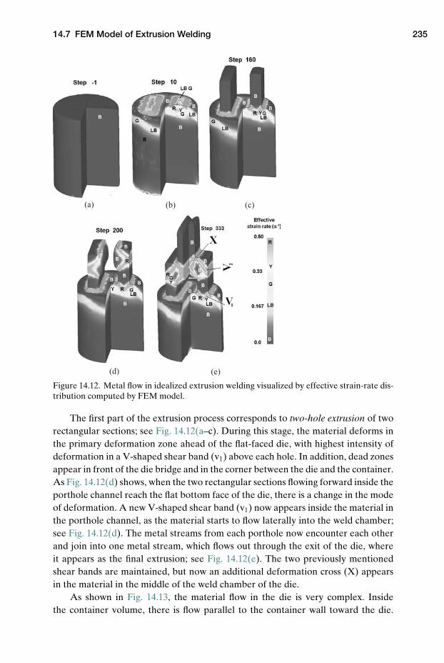
14.7 FEM Model of Extrusion Welding 235
(a) (b)
(d) (e)
(c)
Figure 14.12. Metal flow in idealized extrusion welding visualized by effective strain-rate dis-tribution computed by FEM model.
The first part of the extrusion process corresponds to two-hole extrusion of tworectangular sections; see Fig. 14.12(a–c). During this stage, the material deforms inthe primary deformation zone ahead of the flat-faced die, with highest intensity ofdeformation in a V-shaped shear band (v1) above each hole. In addition, dead zonesappear in front of the die bridge and in the corner between the die and the container.As Fig. 14.12(d) shows, when the two rectangular sections flowing forward inside theporthole channel reach the flat bottom face of the die, there is a change in the modeof deformation. A new V-shaped shear band (v1) now appears inside the material inthe porthole channel, as the material starts to flow laterally into the weld chamber;see Fig. 14.12(d). The metal streams from each porthole now encounter each otherand join into one metal stream, which flows out through the exit of the die, whereit appears as the final extrusion; see Fig. 14.12(e). The two previously mentionedshear bands are maintained, but now an additional deformation cross (X) appearsin the material in the middle of the weld chamber of the die.
As shown in Fig. 14.13, the material flow in the die is very complex. Insidethe container volume, there is flow parallel to the container wall toward the die.
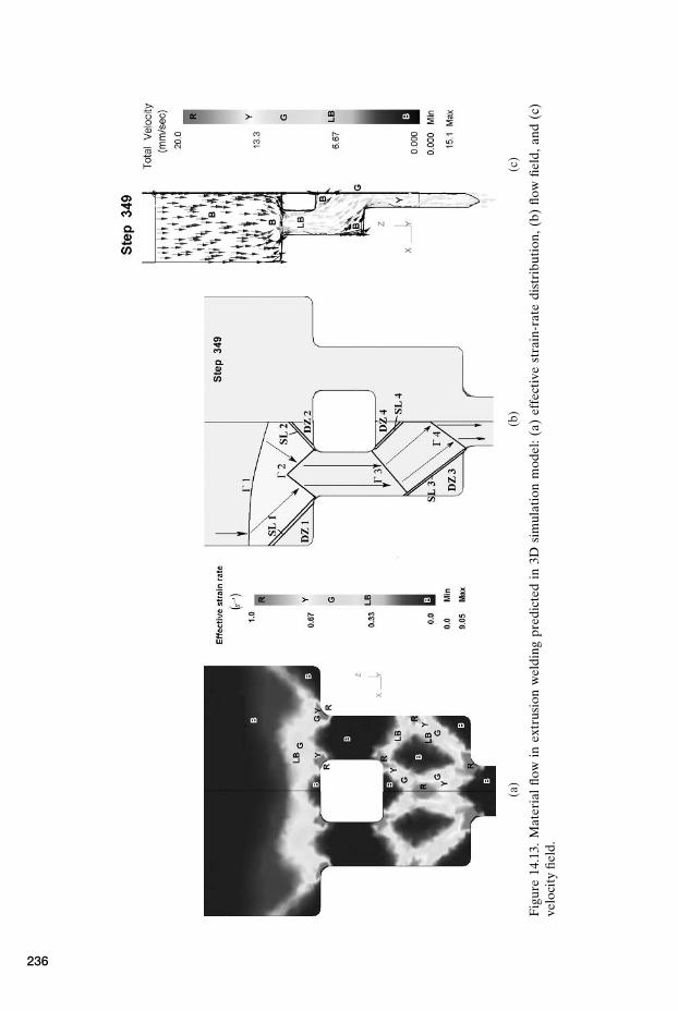
(a)
(b)
(c)
Fig
ure
14.1
3.M
ater
ial
flow
inex
trus
ion
wel
ding
pred
icte
din
3Dsi
mul
atio
nm
odel
:(a)
effe
ctiv
est
rain
-rat
edi
stri
buti
on,(
b)flo
wfie
ld,a
nd(c
)ve
loci
tyfie
ld.
236
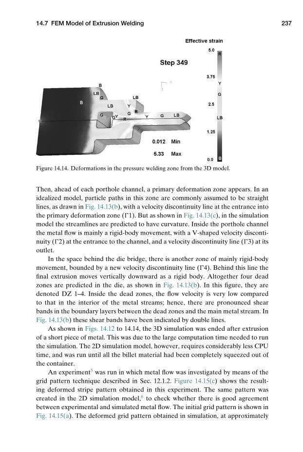
14.7 FEM Model of Extrusion Welding 237
Figure 14.14. Deformations in the pressure welding zone from the 3D model.
Then, ahead of each porthole channel, a primary deformation zone appears. In anidealized model, particle paths in this zone are commonly assumed to be straightlines, as drawn in Fig. 14.13(b), with a velocity discontinuity line at the entrance intothe primary deformation zone (�1). But as shown in Fig. 14.13(c), in the simulationmodel the streamlines are predicted to have curvature. Inside the porthole channelthe metal flow is mainly a rigid-body movement, with a V-shaped velocity disconti-nuity (�2) at the entrance to the channel, and a velocity discontinuity line (�3) at itsoutlet.
In the space behind the die bridge, there is another zone of mainly rigid-bodymovement, bounded by a new velocity discontinuity line (�4). Behind this line thefinal extrusion moves vertically downward as a rigid body. Altogether four deadzones are predicted in the die, as shown in Fig. 14.13(b). In this figure, they aredenoted DZ 1–4. Inside the dead zones, the flow velocity is very low comparedto that in the interior of the metal streams; hence, there are pronounced shearbands in the boundary layers between the dead zones and the main metal stream. InFig. 14.13(b) these shear bands have been indicated by double lines.
As shown in Figs. 14.12 to 14.14, the 3D simulation was ended after extrusionof a short piece of metal. This was due to the large computation time needed to runthe simulation. The 2D simulation model, however, requires considerably less CPUtime, and was run until all the billet material had been completely squeezed out ofthe container.
An experiment5 was run in which metal flow was investigated by means of thegrid pattern technique described in Sec. 12.1.2. Figure 14.15(c) shows the result-ing deformed stripe pattern obtained in this experiment. The same pattern wascreated in the 2D simulation model,6 to check whether there is good agreementbetween experimental and simulated metal flow. The initial grid pattern is shown inFig. 14.15(a). The deformed grid pattern obtained in simulation, at approximately
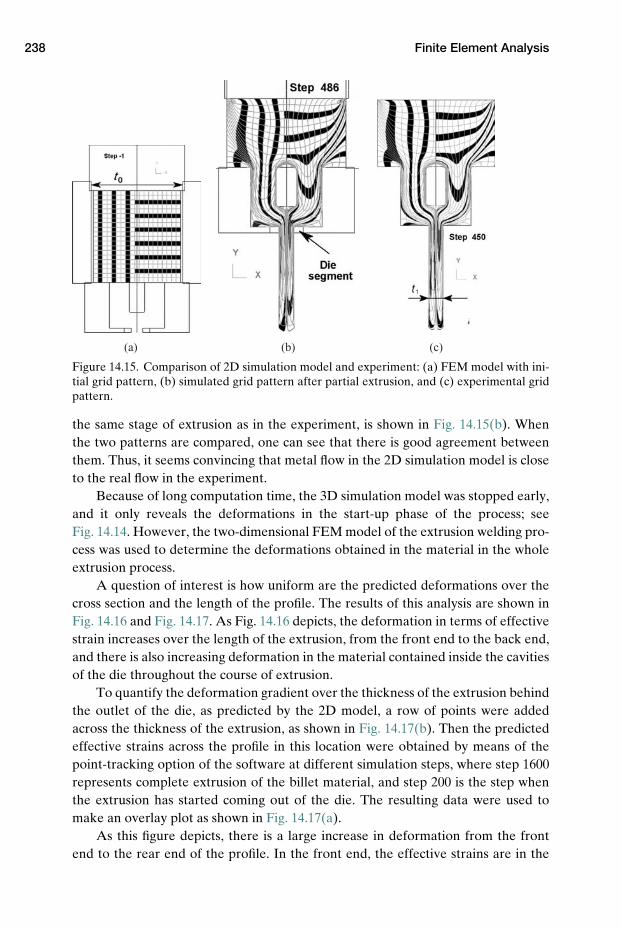
238 Finite Element Analysis
(a) (b) (c)
Figure 14.15. Comparison of 2D simulation model and experiment: (a) FEM model with ini-tial grid pattern, (b) simulated grid pattern after partial extrusion, and (c) experimental gridpattern.
the same stage of extrusion as in the experiment, is shown in Fig. 14.15(b). Whenthe two patterns are compared, one can see that there is good agreement betweenthem. Thus, it seems convincing that metal flow in the 2D simulation model is closeto the real flow in the experiment.
Because of long computation time, the 3D simulation model was stopped early,and it only reveals the deformations in the start-up phase of the process; seeFig. 14.14. However, the two-dimensional FEM model of the extrusion welding pro-cess was used to determine the deformations obtained in the material in the wholeextrusion process.
A question of interest is how uniform are the predicted deformations over thecross section and the length of the profile. The results of this analysis are shown inFig. 14.16 and Fig. 14.17. As Fig. 14.16 depicts, the deformation in terms of effectivestrain increases over the length of the extrusion, from the front end to the back end,and there is also increasing deformation in the material contained inside the cavitiesof the die throughout the course of extrusion.
To quantify the deformation gradient over the thickness of the extrusion behindthe outlet of the die, as predicted by the 2D model, a row of points were addedacross the thickness of the extrusion, as shown in Fig. 14.17(b). Then the predictedeffective strains across the profile in this location were obtained by means of thepoint-tracking option of the software at different simulation steps, where step 1600represents complete extrusion of the billet material, and step 200 is the step whenthe extrusion has started coming out of the die. The resulting data were used tomake an overlay plot as shown in Fig. 14.17(a).
As this figure depicts, there is a large increase in deformation from the frontend to the rear end of the profile. In the front end, the effective strains are in the
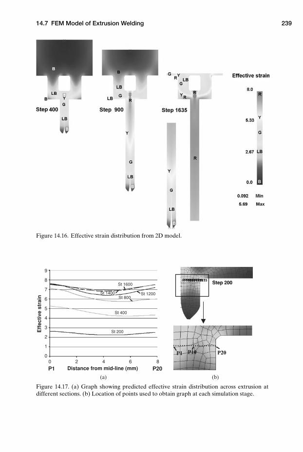
14.7 FEM Model of Extrusion Welding 239
Figure 14.16. Effective strain distribution from 2D model.
9
8
7
6
5
4
3
2
1
00 2 4 6 8
Eff
ecti
ve s
trai
n
Distance from mid-line (mm)P1 P20
P10P1
(a) (b)
St 1600
St 1400 St 1200St 800
St 400
St 200
Figure 14.17. (a) Graph showing predicted effective strain distribution across extrusion atdifferent sections. (b) Location of points used to obtain graph at each simulation stage.
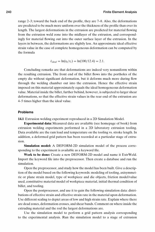
240 Finite Element Analysis
range 2–3; toward the back end of the profile, they are 7–8. Also, the deformationsare predicted to be much more uniform over the thickness of the profile than over itslength. The largest deformations in the extrusion are predicted for material flowingfrom the extrusion weld zone into the midlayer of the extrusion, and correspond-ingly for material flowing out into the outer surface layer of the extrusion. In thelayers in between, the deformations are slightly less. An approximate ideal effectivestrain value in the case of complete homogeneous deformation can be computed bythe formula
εideal = ln(t0/t1) = ln(100/12.4) = 2.1.
Concluding remarks are that deformations are indeed very nonuniform withinthe resulting extrusion. The front end of the billet flows into the portholes of theempty die without significant deformation, but it deforms much more during flowthrough the welding chamber out into the extrusion. Hence the effective strainimposed on this material approximately equals the ideal homogeneous deformationvalue. Material inside the billet, further behind, however, is subjected to larger sheardeformations, so that the effective strain values in the rear end of the extrusion are4–5 times higher than the ideal value.
Problems
14.1 Extrusion welding experiment reproduced in a 2D Simulation Model.Experimental data: Measured data are available (see homepage of book) from
extrusion welding experiments performed in a 2D laboratory extrusion tooling.Data available are the ram load and temperature on the tooling vs. stroke length. Inaddition, a deformed grid pattern has been recorded at a particular stage of extru-sion.
Simulation model: A DEFORM-2D simulation model of the process corre-sponding to the experiment is available as a keyword file.
Work to be done: Create a new DEFORM-2D model and name it ExtrWeld.Import the keyword file into the preprocessor. Then create a database and run thesimulation.
Open the preprocessor, and study how the model has been built. Give a descrip-tion of the model based on the following keywords: modeling of tooling, axisymmet-ric or plane strain model, type of workpiece and die objects, friction model/valueused, constitutive material model of workpiece material, initial thermal condition ofbillet, and tooling.
Open the postprocessor, and use it to gain the following simulation data: distri-butions of effective strain and effective strain rate in the material upon deformation.Use different scaling to depict areas of low and high strain rate. Explain where thereare dead zones, deformation crosses, and shear bands. Comment on where inside theextruding material and the rod the largest deformations are.
Use the simulation model to perform a grid pattern analysis correspondingto the experimental analysis. Run the simulation model to a stage of extrusion
References 241
corresponding to the experiment. Paint black stripes onto simulated pattern to makea pattern corresponding to the experimental one. Comment upon the similaritybetween experiment and simulation.
Find grid elements about to flow, respectively, out of the container and out ofthe die exit, at the instant when the deformed grid pattern is recorded. Trace theseelements back to their initial positions inside the unextruded billet. This should bedone both manually and by use of the software. Insert a grid pattern into the extru-sion at end of simulation. Run the simulations backwards to obtain emptying dia-grams consisting of T and L lines for the extrusion process.
Report: Report the results obtained in your analysis. Discuss them and presentconclusions.
NOTES
1. Uyyuru, R. K.: “Engineering the Friction and Forming Mechanics in Cold AluminiumForming – Use of Modelling Techniques,” Ph.D. thesis, Norwegian Univ. of Science andTechnology (NTNU), 2003, pp. 29–42.
2. http://en.wikipedia.org/wiki/Finite element method.3. Strang, G., and Fix, G.: “An Analysis of he Finite Element Method,” Prentice-Hall, 1973.4. Jo, H. H., Lee, S. K., Jung, C. S., and Kim, B. M.: “A non-steady state FE analysis of Al
tubes hot extrusion by a porthole die,” J. Material Processing Technology Vol. 173, 2006,pp. 223–231.
5. Welo, T, Smaabrekke, A., and Valberg, H.: “Two-dimensional simulation of portholeextrusion,” Aluminium, Vol. 71, No. 1, 1995, pp. 90–94.
6. Valberg, H., Abbas, Y., and Moe, P. T.: “The mechanics of two-dimensional aluminiumextrusion welding investigated by FEA with experiment,” Proc. 9th Int. Conf. Technol-ogy of Plasticity, Gyeongju, Korea, 2008.
REFERENCES
Dixit, P. M., and Dixit, U. S.: “Modeling of Metal Forming and Machining Processes: ByFinite Element and Soft Computing Methods,” Springer-Verlag, 2008.
Kobayashi, S.: “Metal Forming and the Finite Element Method,” Oxford Univ. Press, NewYork, 1989.
Nee, A. Y. C., Ong, S. K., and Wang, Y. G.: “Computer Applications in Near Net-ShapeOperations,” Springer-Verlag, 1999.
Uyyuru, R. K.: “Engineering the Friction and Forming Mechanics in Cold Aluminium Form-ing – Use of Modelling Techniques,” Ph.D. thesis, Norwegian Univ. of Science and Tech-nology (NTNU), 2003, pp. 29–42.
http://www.deform.com/.http://www.transvalor.com/forge.php.http://www.mscsoftware.com/products/superforge support.cfm?PI=28&Q=396&Z=404&
Y=420.http://www.qform3d.com/en/2.html.http://www.ansys.com/products/default.asp.http://www.simulia.com/products/unified fea.html.http://www.ls-dyna.com/.http://www.esi-group.com/products/metal-forming.
15 FEA of Technological Tests
Use of FEM analysis for the study of the mechanics of some important technologicaltest methods will be treated in this chapter. Detailed knowledge of the deformingconditions in such tests is crucial when they are to be used to collect precise materialdata, such as, for example, flow stress data for a particular alloy.
Tensile testing of round specimens is first considered. FEA predicts nonuniformdeformation across the thinnest neck in the specimen, and experimental grid patternanalysis confirms this; the largest deformation occurs at the center of the neck. Thus,in reality one assumption in Bridgman’s correction analysis fails. Because of this,for metals exhibiting strain hardening, it can be shown that in tensile testing it isappropriate to perform a larger correction of the flow stress than that proposed byBridgman.
Cylinder compression testing is then subjected to an in-depth analysis. First, it isshown how experimental grid pattern analysis, supported by inverse FEM modeling,can be used for finding an approximate friction value in the compression test. There-after, FEA is used to map internal deformations inside cylinders being compressedwith friction, so that overfolding of the side of the cylinder occurs.
After this, the friction effects on the compression load are investigated usingFEA. It is shown that friction effects are reduced as the cylinder height is increased.Thus, it can be recommended to use high, slender cylinders in this test (specimenswith aspect ratio in the range 1.5–2) when flow stress data are to be collected.
Finally, the deformational behavior of the specimen in shearing is investigatedwith help of FEA, supported by use of experimental grid pattern techniques. Thisshows the interesting potential of this method, as a test that creates very high strainand strain rates in the material and at the same time allows flow stress data to bededuced from the load–stroke curve obtained in the test.
15.1 Tensile Testing
The mechanics of the tensile test and use of it to acquire the flow curve of a materialwere thoroughly discussed in Ch. 7. It is commonly observed that the flow curvesobtained in tensile and in compressive testing may differ. After the onset of necking
242
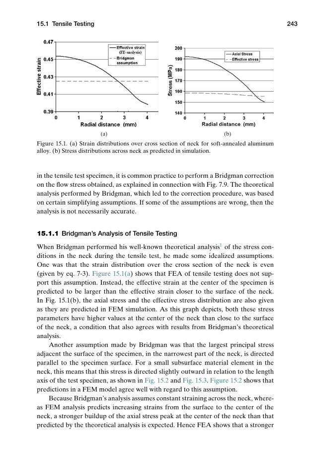
15.1 Tensile Testing 243
(a) (b)
Figure 15.1. (a) Strain distributions over cross section of neck for soft-annealed aluminumalloy. (b) Stress distributions across neck as predicted in simulation.
in the tensile test specimen, it is common practice to perform a Bridgman correctionon the flow stress obtained, as explained in connection with Fig. 7.9. The theoreticalanalysis performed by Bridgman, which led to the correction procedure, was basedon certain simplifying assumptions. If some of the assumptions are wrong, then theanalysis is not necessarily accurate.
15.1.1 Bridgman’s Analysis of Tensile Testing
When Bridgman performed his well-known theoretical analysis1 of the stress con-ditions in the neck during the tensile test, he made some idealized assumptions.One was that the strain distribution over the cross section of the neck is even(given by eq. 7-3). Figure 15.1(a) shows that FEA of tensile testing does not sup-port this assumption. Instead, the effective strain at the center of the specimen ispredicted to be larger than the effective strain closer to the surface of the neck.In Fig. 15.1(b), the axial stress and the effective stress distribution are also givenas they are predicted in FEM simulation. As this graph depicts, both these stressparameters have higher values at the center of the neck than close to the surfaceof the neck, a condition that also agrees with results from Bridgman’s theoreticalanalysis.
Another assumption made by Bridgman was that the largest principal stressadjacent the surface of the specimen, in the narrowest part of the neck, is directedparallel to the specimen surface. For a small subsurface material element in theneck, this means that this stress is directed slightly outward in relation to the lengthaxis of the test specimen, as shown in Fig. 15.2 and Fig. 15.3. Figure 15.2 shows thatpredictions in a FEM model agree well with regard to this assumption.
Because Bridgman’s analysis assumes constant straining across the neck, where-as FEM analysis predicts increasing strains from the surface to the center of theneck, a stronger buildup of the axial stress peak at the center of the neck than thatpredicted by the theoretical analysis is expected. Hence FEA shows that a stronger
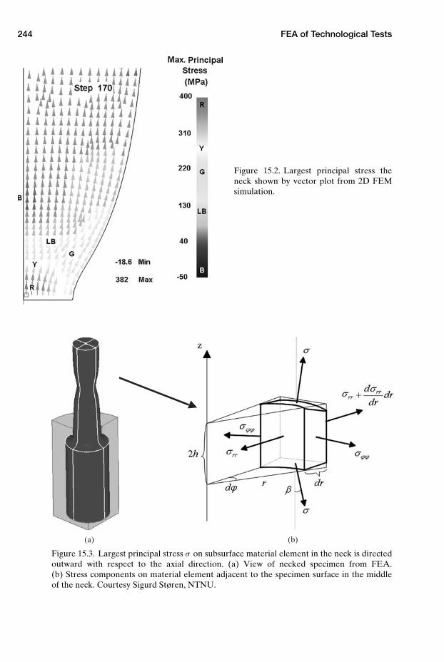
244 FEA of Technological Tests
Figure 15.2. Largest principal stress theneck shown by vector plot from 2D FEMsimulation.
(a) (b)
Figure 15.3. Largest principal stress σ on subsurface material element in the neck is directedoutward with respect to the axial direction. (a) View of necked specimen from FEA.(b) Stress components on material element adjacent to the specimen surface in the middleof the neck. Courtesy Sigurd Støren, NTNU.
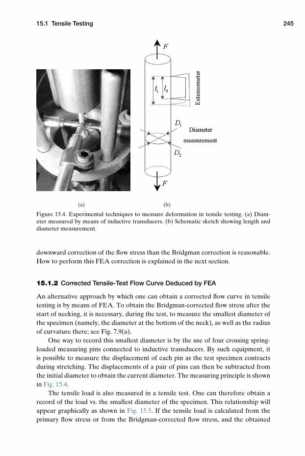
15.1 Tensile Testing 245
(a) (b)
Figure 15.4. Experimental techniques to measure deformation in tensile testing. (a) Diam-eter measured by means of inductive transducers. (b) Schematic sketch showing length anddiameter measurement.
downward correction of the flow stress than the Bridgman correction is reasonable.How to perform this FEA correction is explained in the next section.
15.1.2 Corrected Tensile-Test Flow Curve Deduced by FEA
An alternative approach by which one can obtain a corrected flow curve in tensiletesting is by means of FEA. To obtain the Bridgman-corrected flow stress after thestart of necking, it is necessary, during the test, to measure the smallest diameter ofthe specimen (namely, the diameter at the bottom of the neck), as well as the radiusof curvature there; see Fig. 7.9(a).
One way to record this smallest diameter is by the use of four crossing spring-loaded measuring pins connected to inductive transducers. By such equipment, itis possible to measure the displacement of each pin as the test specimen contractsduring stretching. The displacements of a pair of pins can then be subtracted fromthe initial diameter to obtain the current diameter. The measuring principle is shownin Fig. 15.4.
The tensile load is also measured in a tensile test. One can therefore obtain arecord of the load vs. the smallest diameter of the specimen. This relationship willappear graphically as shown in Fig. 15.5. If the tensile load is calculated from theprimary flow stress or from the Bridgman-corrected flow stress, and the obtained
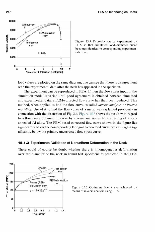
246 FEA of Technological Tests
Figure 15.5. Reproduction of experiment byFEA so that simulated load–diameter curvebecomes identical to corresponding experimen-tal curve.
load values are plotted on the same diagram, one can see that there is disagreementwith the experimental data after the neck has appeared in the specimen.
The experiment can be reproduced in FEA. If then the flow stress input in thesimulation model is varied until good agreement is obtained between simulatedand experimental data, a FEM-corrected flow curve has then been deduced. Thismethod, when applied to find the flow curve, is called inverse analysis, or inversemodeling. Use of it to find the flow curve of a metal was explained previously inconnection with the discussion of Fig. 3.4. Figure 15.6 shows the result with regardto a flow curve obtained this way by inverse analysis in tensile testing of a soft-annealed Al alloy. The FEM-based corrected flow curve shown in the figure liessignificantly below the corresponding Bridgman-corrected curve, which is again sig-nificantly below the primary uncorrected flow stress curve.
15.1.3 Experimental Validation of Nonuniform Deformation in the Neck
There could of course be doubt whether there is inhomogeneous deformationover the diameter of the neck in round test specimens as predicted in the FEA
Figure 15.6. Optimum flow curve achieved bymeans of inverse analysis using FEA.
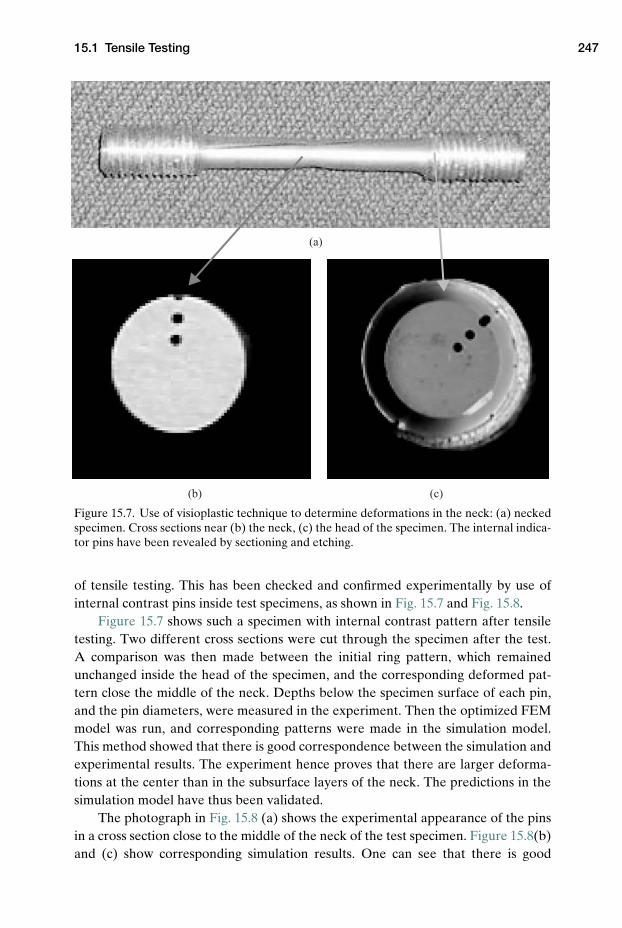
15.1 Tensile Testing 247
(a)
(b) (c)
Figure 15.7. Use of visioplastic technique to determine deformations in the neck: (a) neckedspecimen. Cross sections near (b) the neck, (c) the head of the specimen. The internal indica-tor pins have been revealed by sectioning and etching.
of tensile testing. This has been checked and confirmed experimentally by use ofinternal contrast pins inside test specimens, as shown in Fig. 15.7 and Fig. 15.8.
Figure 15.7 shows such a specimen with internal contrast pattern after tensiletesting. Two different cross sections were cut through the specimen after the test.A comparison was then made between the initial ring pattern, which remainedunchanged inside the head of the specimen, and the corresponding deformed pat-tern close the middle of the neck. Depths below the specimen surface of each pin,and the pin diameters, were measured in the experiment. Then the optimized FEMmodel was run, and corresponding patterns were made in the simulation model.This method showed that there is good correspondence between the simulation andexperimental results. The experiment hence proves that there are larger deforma-tions at the center than in the subsurface layers of the neck. The predictions in thesimulation model have thus been validated.
The photograph in Fig. 15.8 (a) shows the experimental appearance of the pinsin a cross section close to the middle of the neck of the test specimen. Figure 15.8(b)and (c) show corresponding simulation results. One can see that there is good
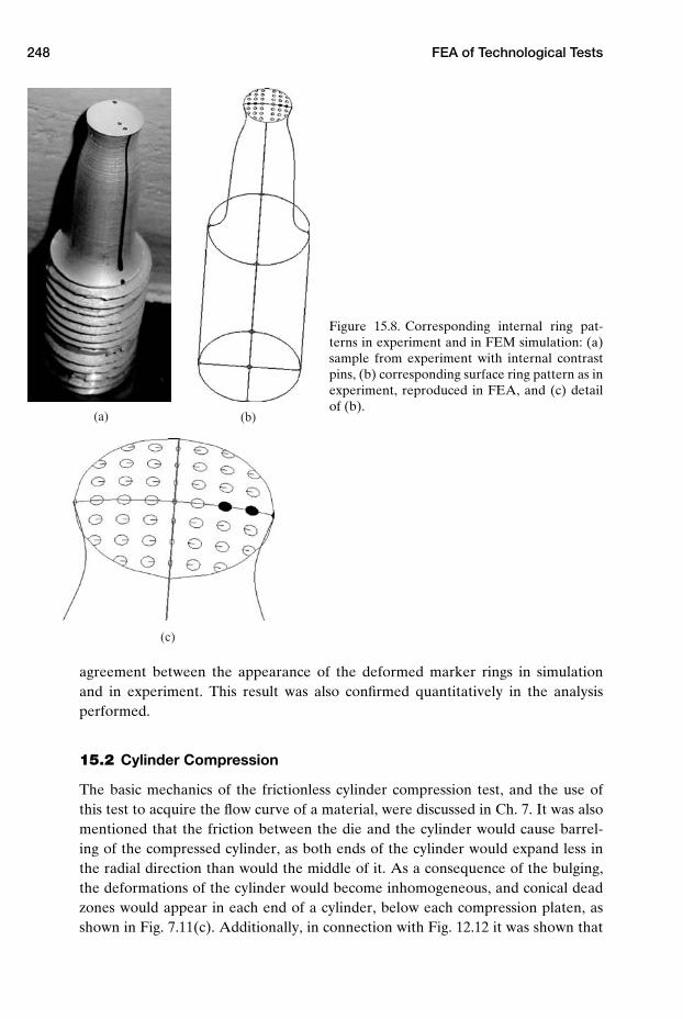
248 FEA of Technological Tests
(a) (b)
(c)
Figure 15.8. Corresponding internal ring pat-terns in experiment and in FEM simulation: (a)sample from experiment with internal contrastpins, (b) corresponding surface ring pattern as inexperiment, reproduced in FEA, and (c) detailof (b).
agreement between the appearance of the deformed marker rings in simulationand in experiment. This result was also confirmed quantitatively in the analysisperformed.
15.2 Cylinder Compression
The basic mechanics of the frictionless cylinder compression test, and the use ofthis test to acquire the flow curve of a material, were discussed in Ch. 7. It was alsomentioned that the friction between the die and the cylinder would cause barrel-ing of the compressed cylinder, as both ends of the cylinder would expand less inthe radial direction than would the middle of it. As a consequence of the bulging,the deformations of the cylinder would become inhomogeneous, and conical deadzones would appear in each end of a cylinder, below each compression platen, asshown in Fig. 7.11(c). Additionally, in connection with Fig. 12.12 it was shown that
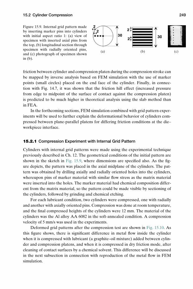
15.2 Cylinder Compression 249
(a) (b) (c)
Figure 15.9. Internal grid pattern madeby inserting marker pins into cylinderswith initial aspect ratio 1: (a) view ofspecimen with inserted axial pins fromthe top, (b) longitudinal section throughspecimen with radially oriented pins,and (c) photograph of specimen shownin (b).
friction between cylinder and compression platen during the compression stroke canbe mapped by inverse analysis based on FEM simulation with the use of markerpoints (small circles) placed on the end face of the cylinder. Finally, in connec-tion with Fig. 14.7, it was shown that the friction hill effect (increased pressurefrom edge to midpoint of the surface of contact against the compression platen)is predicted to be much higher in theoretical analysis using the slab method thanin FEA.
In the forthcoming sections, FEM simulation combined with grid pattern exper-iments will be used to further explain the deformational behavior of cylinders com-pressed between plane-parallel platens for differing friction conditions at the die–workpiece interface.
15.2.1 Compression Experiment with Internal Grid Pattern
Cylinders with internal grid patterns were made using the experimental techniquepreviously described in Ch. 12. The geometrical conditions of the initial pattern areshown in the sketch in Fig. 15.9, where dimensions are specified also. As the fig-ure depicts, the pattern was placed in the axial midplane of the cylinders. The pat-tern was obtained by drilling axially and radially oriented holes into the cylinders,whereupon pins of marker material with similar flow stress as the matrix materialwere inserted into the holes. The marker material had chemical composition differ-ent from the matrix material, so the pattern could be made visible by sectioning ofthe cylinders, followed by grinding and chemical etching.
For each lubricant condition, two cylinders were compressed, one with radiallyand another with axially oriented pins. Compression was done at room temperature,and the final compressed heights of the cylinders were 12 mm. The material of thecylinders was the Al alloy AA 6082 in the soft-annealed condition. A compressionvelocity of 5 mm/s was used in the experiments.
Deformed grid patterns after the compression test are shown in Fig. 15.10. Asthis figure shows, there is significant difference in metal flow inside the cylinderwhen it is compressed with lubricant (a graphite–oil mixture) added between cylin-der and compression platens, and when it is compressed in dry friction mode, aftercleaning of contact surfaces by a chemical solvent. This difference will be discussedin the next subsection in connection with reproduction of the metal flow in FEMsimulation.
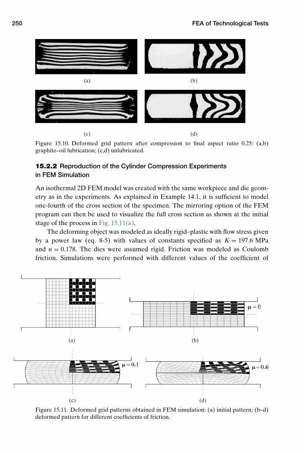
250 FEA of Technological Tests
(a) (b)
(c) (d)
Figure 15.10. Deformed grid pattern after compression to final aspect ratio 0.25: (a,b)graphite–oil lubrication; (c,d) unlubricated.
15.2.2 Reproduction of the Cylinder Compression Experimentsin FEM Simulation
An isothermal 2D FEM model was created with the same workpiece and die geom-etry as in the experiments. As explained in Example 14.1, it is sufficient to modelone-fourth of the cross section of the specimen. The mirroring option of the FEMprogram can then be used to visualize the full cross section as shown at the initialstage of the process in Fig. 15.11(a).
The deforming object was modeled as ideally rigid–plastic with flow stress givenby a power law (eq. 8-5) with values of constants specified as K = 197.6 MPaand n = 0.178. The dies were assumed rigid. Friction was modeled as Coulombfriction. Simulations were performed with different values of the coefficient of
(a) (b)
(c) (d)
Figure 15.11. Deformed grid patterns obtained in FEM simulation: (a) initial pattern; (b–d)deformed pattern for different coefficients of friction.
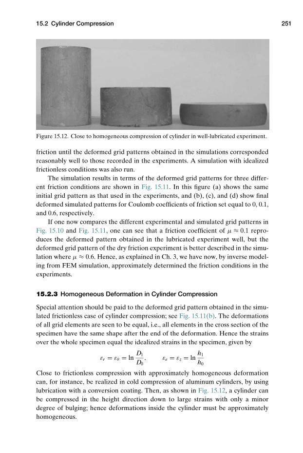
15.2 Cylinder Compression 251
Figure 15.12. Close to homogeneous compression of cylinder in well-lubricated experiment.
friction until the deformed grid patterns obtained in the simulations correspondedreasonably well to those recorded in the experiments. A simulation with idealizedfrictionless conditions was also run.
The simulation results in terms of the deformed grid patterns for three differ-ent friction conditions are shown in Fig. 15.11. In this figure (a) shows the sameinitial grid pattern as that used in the experiments, and (b), (c), and (d) show finaldeformed simulated patterns for Coulomb coefficients of friction set equal to 0, 0.1,and 0.6, respectively.
If one now compares the different experimental and simulated grid patterns inFig. 15.10 and Fig. 15.11, one can see that a friction coefficient of µ ≈ 0.1 repro-duces the deformed pattern obtained in the lubricated experiment well, but thedeformed grid pattern of the dry friction experiment is better described in the simu-lation where µ ≈ 0.6. Hence, as explained in Ch. 3, we have now, by inverse model-ing from FEM simulation, approximately determined the friction conditions in theexperiments.
15.2.3 Homogeneous Deformation in Cylinder Compression
Special attention should be paid to the deformed grid pattern obtained in the simu-lated frictionless case of cylinder compression; see Fig. 15.11(b). The deformationsof all grid elements are seen to be equal, i.e., all elements in the cross section of thespecimen have the same shape after the end of the deformation. Hence the strainsover the whole specimen equal the idealized strains in the specimen, given by
εr = εθ = lnD1
D0, εe = εz = ln
h1
h0
Close to frictionless compression with approximately homogeneous deformationcan, for instance, be realized in cold compression of aluminum cylinders, by usinglubrication with a conversion coating. Then, as shown in Fig. 15.12, a cylinder canbe compressed in the height direction down to large strains with only a minordegree of bulging; hence deformations inside the cylinder must be approximatelyhomogeneous.
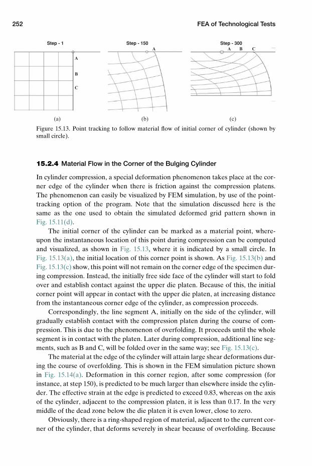
252 FEA of Technological Tests
(a) (b) (c)
Step - 1 Step - 150 Step - 300A B C
A
A
B
C
Figure 15.13. Point tracking to follow material flow of initial corner of cylinder (shown bysmall circle).
15.2.4 Material Flow in the Corner of the Bulging Cylinder
In cylinder compression, a special deformation phenomenon takes place at the cor-ner edge of the cylinder when there is friction against the compression platens.The phenomenon can easily be visualized by FEM simulation, by use of the point-tracking option of the program. Note that the simulation discussed here is thesame as the one used to obtain the simulated deformed grid pattern shown inFig. 15.11(d).
The initial corner of the cylinder can be marked as a material point, where-upon the instantaneous location of this point during compression can be computedand visualized, as shown in Fig. 15.13, where it is indicated by a small circle. InFig. 15.13(a), the initial location of this corner point is shown. As Fig. 15.13(b) andFig. 15.13(c) show, this point will not remain on the corner edge of the specimen dur-ing compression. Instead, the initially free side face of the cylinder will start to foldover and establish contact against the upper die platen. Because of this, the initialcorner point will appear in contact with the upper die platen, at increasing distancefrom the instantaneous corner edge of the cylinder, as compression proceeds.
Correspondingly, the line segment A, initially on the side of the cylinder, willgradually establish contact with the compression platen during the course of com-pression. This is due to the phenomenon of overfolding. It proceeds until the wholesegment is in contact with the platen. Later during compression, additional line seg-ments, such as B and C, will be folded over in the same way; see Fig. 15.13(c).
The material at the edge of the cylinder will attain large shear deformations dur-ing the course of overfolding. This is shown in the FEM simulation picture shownin Fig. 15.14(a). Deformation in this corner region, after some compression (forinstance, at step 150), is predicted to be much larger than elsewhere inside the cylin-der. The effective strain at the edge is predicted to exceed 0.83, whereas on the axisof the cylinder, adjacent to the compression platen, it is less than 0.17. In the verymiddle of the dead zone below the die platen it is even lower, close to zero.
Obviously, there is a ring-shaped region of material, adjacent to the current cor-ner of the cylinder, that deforms severely in shear because of overfolding. Because
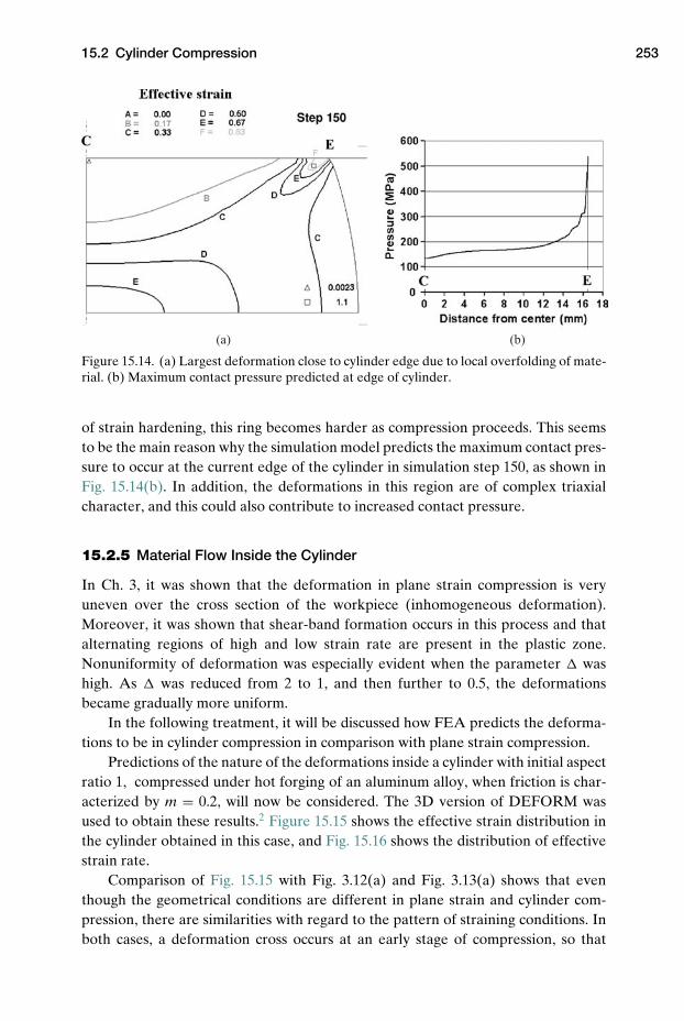
15.2 Cylinder Compression 253
(a) (b)
Figure 15.14. (a) Largest deformation close to cylinder edge due to local overfolding of mate-rial. (b) Maximum contact pressure predicted at edge of cylinder.
of strain hardening, this ring becomes harder as compression proceeds. This seemsto be the main reason why the simulation model predicts the maximum contact pres-sure to occur at the current edge of the cylinder in simulation step 150, as shown inFig. 15.14(b). In addition, the deformations in this region are of complex triaxialcharacter, and this could also contribute to increased contact pressure.
15.2.5 Material Flow Inside the Cylinder
In Ch. 3, it was shown that the deformation in plane strain compression is veryuneven over the cross section of the workpiece (inhomogeneous deformation).Moreover, it was shown that shear-band formation occurs in this process and thatalternating regions of high and low strain rate are present in the plastic zone.Nonuniformity of deformation was especially evident when the parameter � washigh. As � was reduced from 2 to 1, and then further to 0.5, the deformationsbecame gradually more uniform.
In the following treatment, it will be discussed how FEA predicts the deforma-tions to be in cylinder compression in comparison with plane strain compression.
Predictions of the nature of the deformations inside a cylinder with initial aspectratio 1, compressed under hot forging of an aluminum alloy, when friction is char-acterized by m = 0.2, will now be considered. The 3D version of DEFORM wasused to obtain these results.2 Figure 15.15 shows the effective strain distribution inthe cylinder obtained in this case, and Fig. 15.16 shows the distribution of effectivestrain rate.
Comparison of Fig. 15.15 with Fig. 3.12(a) and Fig. 3.13(a) shows that eventhough the geometrical conditions are different in plane strain and cylinder com-pression, there are similarities with regard to the pattern of straining conditions. Inboth cases, a deformation cross occurs at an early stage of compression, so that
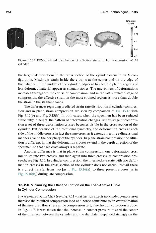
254 FEA of Technological Tests
Figure 15.15. FEM-predicted distribution of effective strain in hot compression of Alcylinder.
the largest deformations in the cross section of the cylinder occur in an X con-figuration. Maximum strain inside the cross is at the center and on the edge ofthe cylinder. In the middle of the cylinder, adjacent to each die platen, regions ofless-deformed material appear as stagnant zones. The unevenness of deformationsincreases throughout the course of compression, and in the last simulated stage ofcompression, the effective strain in the most-strained regions is more than doublethe strain in the stagnant zones.
The differences regarding predicted strain-rate distribution in cylinder compres-sion and in plane strain compression are seen by comparison of Fig. 15.16 withFig. 3.12(b) and Fig. 3.13(b). In both cases, when the specimen has been reducedsufficiently in height, the pattern of deformation changes. At this stage of compres-sion a set of three deformation crosses becomes visible in the cross section of thecylinder. But because of the rotational symmetry, the deformation cross at eachside of the middle cross is in fact the same cross, as it extends in a three-dimensionalmanner around the periphery of the cylinder. In plane strain compression the situa-tion is different, in that the deformation crosses extend in the depth direction of thespecimen, so that each cross always is separate.
Another difference is that in plane strain compression, one deformation crossmultiplies into two crosses, and then again into three crosses, as compression pro-ceeds; see Fig. 3.16. In cylinder compression, the intermediate state with two defor-mation crosses in the cross section of the cylinder does not occur. Instead thereis a direct transfer from two [as in Fig. 15.16(a)] to three present crosses [as inFig. 15.16(b)] during late compression.
15.2.6 Minimizing the Effect of Friction on the Load–Stroke Curvein Cylinder Compression
It was pointed out in Ch. 7 (see Fig. 7.11) that friction effects in cylinder compressionincrease the required compression load and hence contribute to an overestimationof the measured flow stress in the compression test, if no friction correction is done.In Fig. 14.7, it was shown that the increase in contact pressure toward the centerof the interface between the cylinder and the die platen depended strongly on the
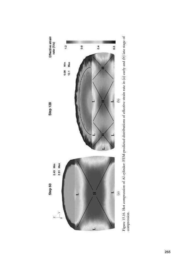
XY
Z
(a)
(b)
Fig
ure
15.1
6.H
otco
mpr
essi
onof
Alc
ylin
der:
FE
M-p
redi
cted
dist
ribu
tion
sof
effe
ctiv
est
rain
rate
in(a
)ea
rly
and
(b)
late
stag
eof
com
pres
sion
.
255
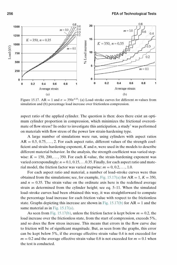
256 FEA of Technological Tests
(a) (b)
Figure 15.17. AR = 1 and σ = 350ε0.35: (a) Load–stroke curves for different m-values fromsimulation and (b) percentage load increase over frictionless compression.
aspect ratio of the applied cylinder. The question is then: does there exist an opti-mum cylinder proportion in compression, which minimizes the frictional overesti-mate of flow stress? In order to investigate this anticipation, a study3 was performedon materials with flow stress of the power law strain-hardening type.
A large number of simulations were run, using cylinders with aspect ratiosAR = 0.5, 0.75, . . . , 2. For each aspect ratio, different values of the strength coef-ficient and strain-hardening exponent, K and n, were used in the models to describedifferent material behavior. In the analysis, the strength coefficient was varied step-wise: K = 150, 200, . . . , 350. For each K-value, the strain-hardening exponent wasvaried correspondingly: n = 0.1, 0.15, . . . 0.35. Finally, for each aspect ratio and mate-rial model, the friction factor was varied stepwise: m = 0, 0.2, . . . , 1.0.
For each aspect ratio and material, a number of load–stroke curves were thusobtained from the simulations; see, for example, Fig. 15.17(a) for AR = 1, K = 350,and n = 0.35. The strain value on the ordinate axis here is the redefined averagestrain as determined from the cylinder height; see eq. 5–11. When the simulatedload–stroke curves had been obtained this way, it was straightforward to computethe percentage load increase for each friction value with respect to the frictionlessstate. Graphs depicting this increase are shown in Fig. 15.17(b) for AR = 1 and thesame material as in Fig. 15.17(a).
As seen from Fig. 15.17(b), unless the friction factor is kept below m = 0.2, theload increase over the frictionless state, from the start of compression, exceeds 5%,and so does the flow stress increase. This means that errors in the flow curve dueto friction will be of significant magnitude. But, as seen from the graphs, this errorcan be kept below 5%, if the average effective strain value 0.4 is not exceeded form = 0.2 and the average effective strain value 0.8 is not exceeded for m = 0.1 whenthe test is conducted.
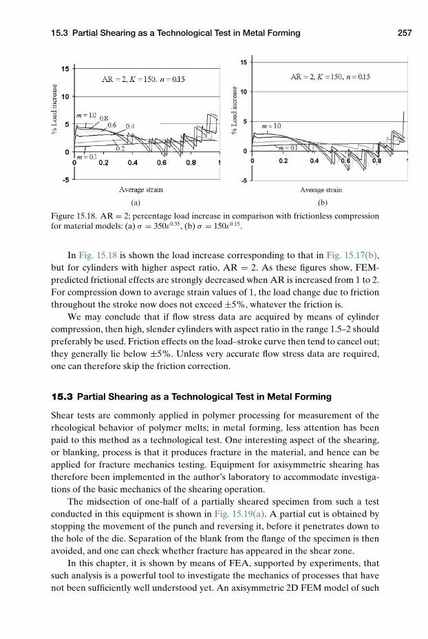
15.3 Partial Shearing as a Technological Test in Metal Forming 257
(a) (b)
Figure 15.18. AR = 2; percentage load increase in comparison with frictionless compressionfor material models: (a) σ = 350ε0.35, (b) σ = 150ε0.15.
In Fig. 15.18 is shown the load increase corresponding to that in Fig. 15.17(b),but for cylinders with higher aspect ratio, AR = 2. As these figures show, FEM-predicted frictional effects are strongly decreased when AR is increased from 1 to 2.For compression down to average strain values of 1, the load change due to frictionthroughout the stroke now does not exceed ±5%, whatever the friction is.
We may conclude that if flow stress data are acquired by means of cylindercompression, then high, slender cylinders with aspect ratio in the range 1.5–2 shouldpreferably be used. Friction effects on the load–stroke curve then tend to cancel out;they generally lie below ±5%. Unless very accurate flow stress data are required,one can therefore skip the friction correction.
15.3 Partial Shearing as a Technological Test in Metal Forming
Shear tests are commonly applied in polymer processing for measurement of therheological behavior of polymer melts; in metal forming, less attention has beenpaid to this method as a technological test. One interesting aspect of the shearing,or blanking, process is that it produces fracture in the material, and hence can beapplied for fracture mechanics testing. Equipment for axisymmetric shearing hastherefore been implemented in the author’s laboratory to accommodate investiga-tions of the basic mechanics of the shearing operation.
The midsection of one-half of a partially sheared specimen from such a testconducted in this equipment is shown in Fig. 15.19(a). A partial cut is obtained bystopping the movement of the punch and reversing it, before it penetrates down tothe hole of the die. Separation of the blank from the flange of the specimen is thenavoided, and one can check whether fracture has appeared in the shear zone.
In this chapter, it is shown by means of FEA, supported by experiments, thatsuch analysis is a powerful tool to investigate the mechanics of processes that havenot been sufficiently well understood yet. An axisymmetric 2D FEM model of such
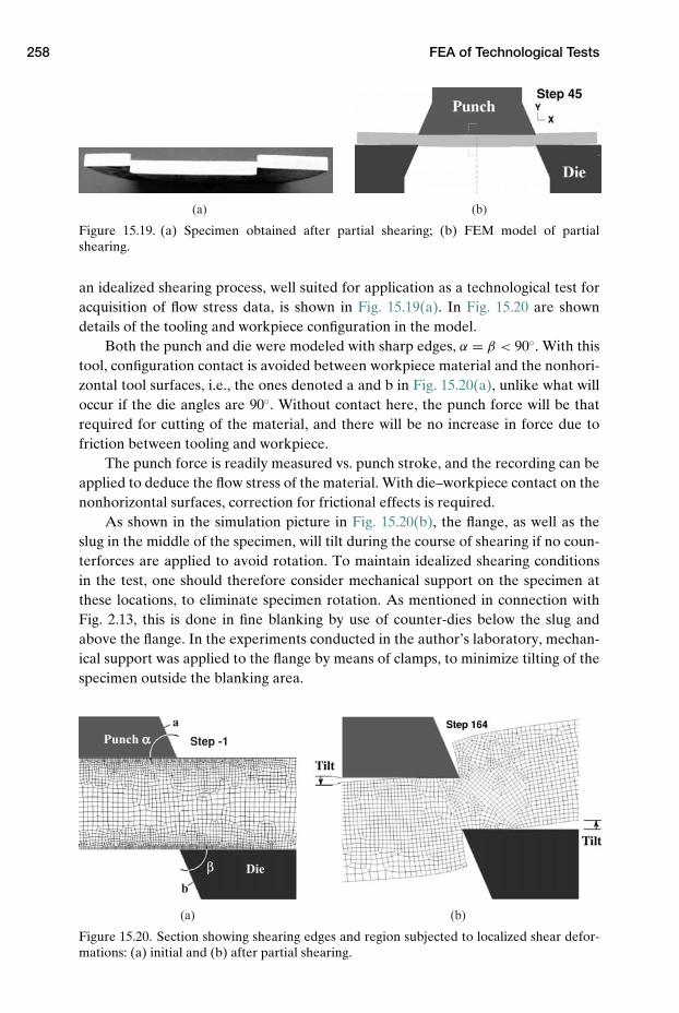
258 FEA of Technological Tests
(a) (b)
Figure 15.19. (a) Specimen obtained after partial shearing; (b) FEM model of partialshearing.
an idealized shearing process, well suited for application as a technological test foracquisition of flow stress data, is shown in Fig. 15.19(a). In Fig. 15.20 are showndetails of the tooling and workpiece configuration in the model.
Both the punch and die were modeled with sharp edges, α = β < 90◦. With thistool, configuration contact is avoided between workpiece material and the nonhori-zontal tool surfaces, i.e., the ones denoted a and b in Fig. 15.20(a), unlike what willoccur if the die angles are 90◦. Without contact here, the punch force will be thatrequired for cutting of the material, and there will be no increase in force due tofriction between tooling and workpiece.
The punch force is readily measured vs. punch stroke, and the recording can beapplied to deduce the flow stress of the material. With die–workpiece contact on thenonhorizontal surfaces, correction for frictional effects is required.
As shown in the simulation picture in Fig. 15.20(b), the flange, as well as theslug in the middle of the specimen, will tilt during the course of shearing if no coun-terforces are applied to avoid rotation. To maintain idealized shearing conditionsin the test, one should therefore consider mechanical support on the specimen atthese locations, to eliminate specimen rotation. As mentioned in connection withFig. 2.13, this is done in fine blanking by use of counter-dies below the slug andabove the flange. In the experiments conducted in the author’s laboratory, mechan-ical support was applied to the flange by means of clamps, to minimize tilting of thespecimen outside the blanking area.
Punch αα
β Die
b
a
Step -1
(a) (b)
Figure 15.20. Section showing shearing edges and region subjected to localized shear defor-mations: (a) initial and (b) after partial shearing.
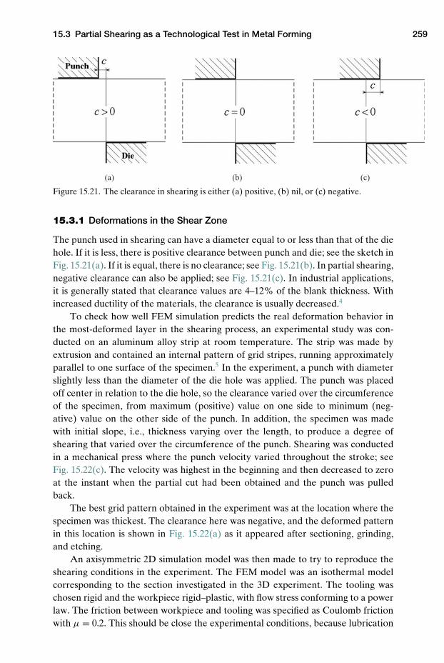
15.3 Partial Shearing as a Technological Test in Metal Forming 259
(a) (b) (c)
Figure 15.21. The clearance in shearing is either (a) positive, (b) nil, or (c) negative.
15.3.1 Deformations in the Shear Zone
The punch used in shearing can have a diameter equal to or less than that of the diehole. If it is less, there is positive clearance between punch and die; see the sketch inFig. 15.21(a). If it is equal, there is no clearance; see Fig. 15.21(b). In partial shearing,negative clearance can also be applied; see Fig. 15.21(c). In industrial applications,it is generally stated that clearance values are 4–12% of the blank thickness. Withincreased ductility of the materials, the clearance is usually decreased.4
To check how well FEM simulation predicts the real deformation behavior inthe most-deformed layer in the shearing process, an experimental study was con-ducted on an aluminum alloy strip at room temperature. The strip was made byextrusion and contained an internal pattern of grid stripes, running approximatelyparallel to one surface of the specimen.5 In the experiment, a punch with diameterslightly less than the diameter of the die hole was applied. The punch was placedoff center in relation to the die hole, so the clearance varied over the circumferenceof the specimen, from maximum (positive) value on one side to minimum (neg-ative) value on the other side of the punch. In addition, the specimen was madewith initial slope, i.e., thickness varying over the length, to produce a degree ofshearing that varied over the circumference of the punch. Shearing was conductedin a mechanical press where the punch velocity varied throughout the stroke; seeFig. 15.22(c). The velocity was highest in the beginning and then decreased to zeroat the instant when the partial cut had been obtained and the punch was pulledback.
The best grid pattern obtained in the experiment was at the location where thespecimen was thickest. The clearance here was negative, and the deformed patternin this location is shown in Fig. 15.22(a) as it appeared after sectioning, grinding,and etching.
An axisymmetric 2D simulation model was then made to try to reproduce theshearing conditions in the experiment. The FEM model was an isothermal modelcorresponding to the section investigated in the 3D experiment. The tooling waschosen rigid and the workpiece rigid–plastic, with flow stress conforming to a powerlaw. The friction between workpiece and tooling was specified as Coulomb frictionwith µ = 0.2. This should be close the experimental conditions, because lubrication
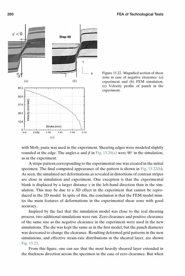
260 FEA of Technological Tests
(a) (b)
(c)
Figure 15.22. Magnified section of shearzone in case of negative clearance: (a)experiment and (b) FEM simulation.(c) Velocity profile of punch in theexperiment.
with MoS2 paste was used in the experiment. Shearing edges were modeled slightlyrounded at the edge. The angles α and β in Fig. 15.20(a) were 90◦ in the simulation,as in the experiment.
A stripe pattern corresponding to the experimental one was created in the initialspecimen. The final computed appearance of the pattern is shown in Fig. 15.22(b).As seen, the simulated net deformations as revealed in distortions of contrast stripesare close in simulation and experiment. One exception is that the experimentalblank is displaced by a larger distance x in the left-hand direction than in the sim-ulation. This may be due to a 3D effect in the experiment that cannot be repro-duced in the 2D model. In spite of this, the conclusion is that the FEM model mim-ics the main features of deformations in the experimental shear zone with goodaccuracy.
Inspired by the fact that the simulation model was close to the real shearingprocess, two additional simulations were run. Zero clearance and positive clearanceof the same size as the negative clearance in the experiment were used in the newsimulations. The die was kept the same as in the first model, but the punch diameterwas decreased to change the clearance. Resulting deformed grid patterns in the newsimulations, and effective strain-rate distributions in the sheared layer, are shownFig. 15.23.
From this figure, one can see that the most heavily sheared layer extended inthe thickness direction across the specimen in the case of zero clearance. But when
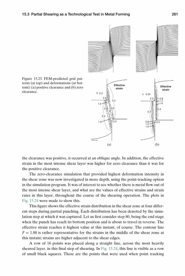
15.3 Partial Shearing as a Technological Test in Metal Forming 261
Effective strain
0.40.4
0.8
0.8
1.2
1.22.0
2.0
3.24
1.6
1.6
Effective strain
0.4
0.80.8
1.21.2
2.0
2.0
2.3
1.6
1.6
0.4
(a) (b)
Figure 15.23. FEM-predicted grid pat-terns (at top) and deformations (at bot-tom): (a) positive clearance and (b) zeroclearance.
the clearance was positive, it occurred at an oblique angle. In addition, the effectivestrain in the most intense shear layer was higher for zero clearance than it was forthe positive clearance.
The zero-clearance simulation that provided highest deformation intensity inthe shear zone was now investigated in more depth, using the point-tracking optionin the simulation program. It was of interest to see whether there is metal flow out ofthe most intense shear layer, and what are the values of effective strains and strainrates in this layer, throughout the course of the shearing operation. The plots inFig. 15.24 were made to show this.
This figure shows the effective strain distribution in the shear zone at four differ-ent steps during partial punching. Each distribution has been denoted by the simu-lation step at which it was captured. Let us first consider step 80, being the end stagewhen the punch has reach its bottom position and is about to travel in reverse. Theeffective strain reaches it highest value at this instant, of course. The contour lineF = 1.88 is rather representative for the strains in the middle of the shear zone atthis instant; strains are higher adjacent to the shear edges.
A row of 16 points was placed along a straight line, across the most heavilysheared layer, in this final step of shearing. In Fig. 15.24, this line is visible as a rowof small black squares. These are the points that were used when point tracking
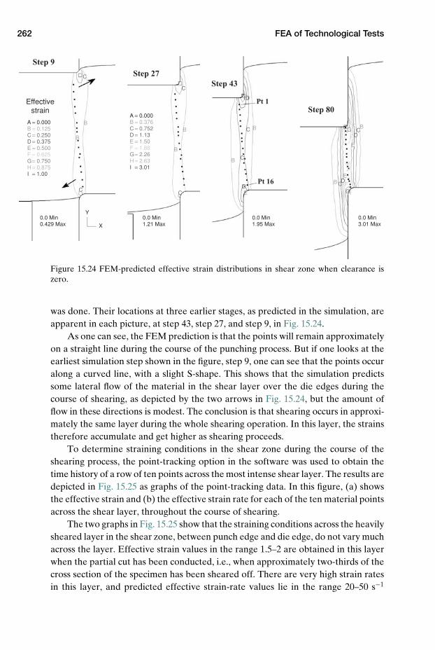
262 FEA of Technological Tests
Step 9
Effective strain
A = 0.000 B = 0.125 C = 0.250 D = 0.375 E = 0.500 F = 0.625 G = 0.750 H = 0.875 I = 1.00
B
B
C
C
Y
X
0.0 Min 0.429 Max
Step 27
A = 0.000 B = 0.376 C = 0.752 D = 1.13 E = 1.50 F = 1.88 G = 2.26 H = 2.63 I = 3.01
B
B
C
C
0.0 Min 1.21 Max
Step 43
Pt 1
Pt 16
B
B
D
D
C
C
E
E
0.0 Min 1.95 Max
Step 80
B
B
G
G
D
D
C
C
H
H
E
E
F
FF
F
0.0 Min 3.01 Max
Figure 15.24 FEM-predicted effective strain distributions in shear zone when clearance iszero.
was done. Their locations at three earlier stages, as predicted in the simulation, areapparent in each picture, at step 43, step 27, and step 9, in Fig. 15.24.
As one can see, the FEM prediction is that the points will remain approximatelyon a straight line during the course of the punching process. But if one looks at theearliest simulation step shown in the figure, step 9, one can see that the points occuralong a curved line, with a slight S-shape. This shows that the simulation predictssome lateral flow of the material in the shear layer over the die edges during thecourse of shearing, as depicted by the two arrows in Fig. 15.24, but the amount offlow in these directions is modest. The conclusion is that shearing occurs in approxi-mately the same layer during the whole shearing operation. In this layer, the strainstherefore accumulate and get higher as shearing proceeds.
To determine straining conditions in the shear zone during the course of theshearing process, the point-tracking option in the software was used to obtain thetime history of a row of ten points across the most intense shear layer. The results aredepicted in Fig. 15.25 as graphs of the point-tracking data. In this figure, (a) showsthe effective strain and (b) the effective strain rate for each of the ten material pointsacross the shear layer, throughout the course of shearing.
The two graphs in Fig. 15.25 show that the straining conditions across the heavilysheared layer in the shear zone, between punch edge and die edge, do not vary muchacross the layer. Effective strain values in the range 1.5–2 are obtained in this layerwhen the partial cut has been conducted, i.e., when approximately two-thirds of thecross section of the specimen has been sheared off. There are very high strain ratesin this layer, and predicted effective strain-rate values lie in the range 20–50 s−1
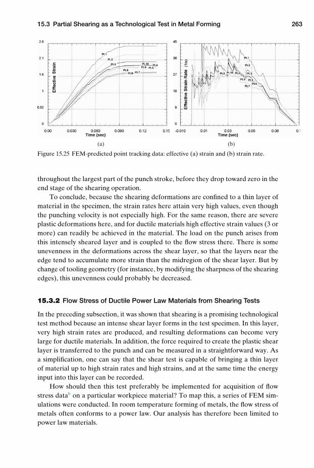
15.3 Partial Shearing as a Technological Test in Metal Forming 263
(a) (b)
Figure 15.25 FEM-predicted point tracking data: effective (a) strain and (b) strain rate.
throughout the largest part of the punch stroke, before they drop toward zero in theend stage of the shearing operation.
To conclude, because the shearing deformations are confined to a thin layer ofmaterial in the specimen, the strain rates here attain very high values, even thoughthe punching velocity is not especially high. For the same reason, there are severeplastic deformations here, and for ductile materials high effective strain values (3 ormore) can readily be achieved in the material. The load on the punch arises fromthis intensely sheared layer and is coupled to the flow stress there. There is someunevenness in the deformations across the shear layer, so that the layers near theedge tend to accumulate more strain than the midregion of the shear layer. But bychange of tooling geometry (for instance, by modifying the sharpness of the shearingedges), this unevenness could probably be decreased.
15.3.2 Flow Stress of Ductile Power Law Materials from Shearing Tests
In the preceding subsection, it was shown that shearing is a promising technologicaltest method because an intense shear layer forms in the test specimen. In this layer,very high strain rates are produced, and resulting deformations can become verylarge for ductile materials. In addition, the force required to create the plastic shearlayer is transferred to the punch and can be measured in a straightforward way. Asa simplification, one can say that the shear test is capable of bringing a thin layerof material up to high strain rates and high strains, and at the same time the energyinput into this layer can be recorded.
How should then this test preferably be implemented for acquisition of flowstress data6 on a particular workpiece material? To map this, a series of FEM sim-ulations were conducted. In room temperature forming of metals, the flow stress ofmetals often conforms to a power law. Our analysis has therefore been limited topower law materials.
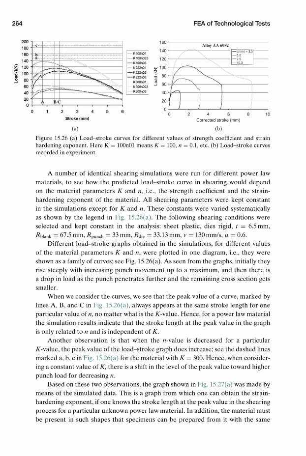
264 FEA of Technological Tests
160
140
120
100
80
60
40
20
00 2 4 6 8 10
Corrected stroke (mm)
Load
(kN
)
Alloy AA 6082t(mm) = 3.3 5.2 7.5 10.3
(a) (b)
Figure 15.26 (a) Load–stroke curves for different values of strength coefficient and strainhardening exponent. Here K = 100n01 means K = 100, n = 0.1, etc. (b) Load–stroke curvesrecorded in experiment.
A number of identical shearing simulations were run for different power lawmaterials, to see how the predicted load–stroke curve in shearing would dependon the material parameters K and n, i.e., the strength coefficient and the strain-hardening exponent of the material. All shearing parameters were kept constantin the simulations except for K and n. These constants were varied systematicallyas shown by the legend in Fig. 15.26(a). The following shearing conditions wereselected and kept constant in the analysis: sheet plastic, dies rigid, t = 6.5 mm,Rblank = 67.5 mm, Rpunch = 33 mm, Rdie = 33.13 mm, v = 130 mm/s, µ = 0.6.
Different load–stroke graphs obtained in the simulations, for different valuesof the material parameters K and n, were plotted in one diagram, i.e., they wereshown as a family of curves; see Fig. 15.26(a). As seen from the graphs, initially theyrise steeply with increasing punch movement up to a maximum, and then there isa drop in load as the punch penetrates further and the remaining cross section getssmaller.
When we consider the curves, we see that the peak value of a curve, marked bylines A, B, and C in Fig. 15.26(a), always appears at the same stroke length for oneparticular value of n, no matter what is the K-value. Hence, for a power law materialthe simulation results indicate that the stroke length at the peak value in the graphis only related to n and is independent of K.
Another observation is that when the n-value is decreased for a particularK-value, the peak value of the load–stroke graph does increase; see the dashed linesmarked a, b, c in Fig. 15.26(a) for the material with K = 300. Hence, when consider-ing a constant value of K, there is a shift in the level of the peak value toward higherpunch load for decreasing n.
Based on these two observations, the graph shown in Fig. 15.27(a) was made bymeans of the simulated data. This is a graph from which one can obtain the strain-hardening exponent, if one knows the stroke length at the peak value in the shearingprocess for a particular unknown power law material. In addition, the material mustbe present in such shapes that specimens can be prepared from it with the same

Problems 265
Figure 15.27 Graphs obtained from simulation to deduce (a) n-value and (b) K-value in sheartesting.
thickness as the specimen used in the FEA. In a corresponding way, the curve shownin Fig. 15.27(b) was made from the simulation data. This graph is used to determinethe K-value of the material after the n-value has been determined from the firstgraph. Hence, we have arrived at a possible procedure for obtaining the flow stressrelationship for a power law strain-hardening material, by simple means – from ameasured load–stroke curve, in a partial shearing test.
Experimentally recorded load–stroke curves for specimens of different thick-ness made from one material are shown in Fig. 15.26(b).
The proposed test is a cheap and rapid one for testing sheet or plate materials.Flat pieces can be tested quickly without cumbersome and expensive preparationof specimens. Data treatment, when the procedure is applied for determination ofthe K and n values of power law materials, is also easy and rapid. Future work onthis topic will be conducted in our laboratory to map the accuracy of the techniqueproposed and to study thermal and strain-rate effects in the test. It is obvious thatthe relations found in this preliminary FEA might be better founded by means oftheoretical analysis. Such work will therefore be welcomed.
Problems
15.1 ACQUISITION OF FLOW STRESS DATA FOR AN ALLOY BYTENSILE TESTING AND CYLINDER COMPRESSION AT ROOMTEMPERATURE
Material: Tensile test and compression test specimens were made from acast and homogenized AA 6082 aluminum alloy billet. The specimens were soft-annealed by heating to a temperature of 420◦C in a furnace. The specimens werekept at this temperature for an hour and were then cooled slowly to 250◦C in thefurnace. After this, the specimens were cooled further to room temperature in air.
Tensile testing: The test was run in a conventional tensile test machine, with acrosshead speed of 10 mm/s. The initial diameter of the specimen was 9.98 mm, and
266 FEA of Technological Tests
the change in diameter was recorded vs. tensile force. Recorded data are availablein a spreadsheet called Test Data.
Compression testing: Tests were run in a Gleeble machine at constant strainrates of 1 and 10 1/s, respectively. Compression force vs. stroke was recorded. Pri-mary data from the tests are available in the Excel spreadsheet called Test Data.The initial cylinder had a diameter of 10 mm and a height of 20 mm.
FEM simulation: An optimized FEM simulation model of the tensile test isavailable. In the model, the flow stress has been chosen so that it provides approxi-mately the same load–diameter curve as in the experiment.
Work to be done by each student group (consisting of two members):
1. Create your own FEM model of tensile testing on the basis of a tutorialprovided. The material model to be used is σ = 197.6ε0.178. Run the simula-tion. Then use the DEFORM-2D postprocessor to obtain the various stresscomponents across the radius of the neck. This is to be done in a late simula-tion step after necking has become clearly visible, but before the specimenthins down too much in the neck. Plot all stress components and the effec-tive stress across the neck in the same diagram. Make a corresponding plotof the effective strain distribution across the neck. Comment on whetherdeformations are predicted to be uniform over the neck. Discuss what dataare of importance when one wants to obtain the optimum flow curve froma tensile test experiment.
2. An optimized FEM model with flow stress data, corresponding to the ten-sile test run in the laboratory, is available as a keyword file Tens Test Opt.Make your own FEM model on the basis of this file. Then use the model toachieve the simulated force vs. diameter diagram. Check to what extent themodel reproduces the load–diameter response as it was determined in theexperiment.
3. Obtain the flow stress data used in the optimized FEM model, and comparethem with the flow stress data obtained directly from the experiments.
4. Use the optimized FEM model to determine strain-rate conditions in thethinnest portion of the tensile test specimen during the test.
5. On the basis of the obtained results, discuss the constitutive behavior ofthe applied material. Is there reasonable agreement between the flow stressobtained in tensile testing and the corresponding flow stress obtained incompression testing?
6. Write a report on your work (one report for each group consisting of twostudents).
NOTES
1. Bridgman, P. W.: “Stress distribution in the neck of a tension specimen,” Trans. Amer.Soc. Metals, Vol. 32, 1944, p. 553.
2. Mjoen, H. R.: “Analysis of Hot Closed-Die Forging of a Commercial Al Alloy” (in Nor-wegian), M.Sc. thesis, Norwegian Univ. of Science and Technology (NTNU), 2002.

References 267
3. Jesnes, G.: “FEM-analysis of compression test,” unpublished work, Internal report, IPM,NTNU, June 2005.
4. Vaz, M., and Bressan, J. D.: “A computational approach to blanking processes,” J. Mate-rial Processing Technology, Vol. 125–126, 2002, pp. 206–212.
5. Khan, Y. A., Ganesan, S. M., Valberg, H., Moe, P. T., and Hansen, A. W.: “Deforma-tion conditions in conventional shearing dependent on geometrical condition of tooling,”Proc. 11th Int. Esaform Conf. on Material Forming, Lyon, France, 2008.
6. Ganesan, S. M., Khan, Y. A., Valberg, H., Moe, P. T., and Hansen, A. W.: “Shearingapplied as test method for acquisition of flow stress data at high strains and strain rates,”Proc. 11th Int. Esaform Conf. on Material Forming, Lyon, France, 2008.
REFERENCES
Davis, J. R.: “Tensile Testing,” ASM Int., Metals Park, Ohio, 2004.Pohlandt, K.: “Materials Testing for the Metal Forming Industry,” Springer-Verlag, 1989.Wright, T. W.: “The Physics and Mathematics of Adiabatic Shear Bands,” Cambridge Univ.
Press, 2002.
16 Forging
The classification system for metal forming processes shown in Fig. 2.1 partitions theforging processes into three different groups: open-die forging, closed-die forging,and impact extrusion. In reality, open-die forging consists of a number of differ-ent subprocesses, in each of which considerable parts of the workpiece are formedfreely, without full contact with the dies; see, for instance, cogging, as shown inFig. 2.2(c). Closed-die forging, on the other hand, refers to forging between dies,where at the end of forging, either the entire workpiece is confined in a closed spacebetween the dies, or an amount of excess material is used, which flows out of theflash gap; see Fig. 2.3(b). When flash is formed, the process is most commonly calledclosed-die forging. When there is no flash, the process is called precision forging,flashless forging, or zero-loss forging. Impact extrusion, such as forward and back-ward cup extrusion, is also described in Ch. 2; see Fig. 2.4. Both are commonly clas-sified as forging processes. In addition, many more exotic forging processes havebeen developed over the years.
In this chapter, some practical aspects of importance in closed-die forging pro-cesses will be considered. First, the concept of forgeability will be discussed. Thenthe implications of this concept for forging practice will be dealt with, such as selec-tion of forging temperature and possible shapes of forgings. A common classifica-tion system for forged components will also be presented. After this, commonly useddesign principles in multistep forging processes will be discussed. The characteris-tics of the load–stroke curve in closed-die forging will be described, and the causesof characteristic flow-related forging defects, such as laps (folds), commonly presentin forging will be discussed. Finally, common flash gap designs applied in closed-dieforging will be considered.
16.1 Forgeability
In forging, the metal is pressed into the die cavity, and should completely fill thecavity a short while before forging is ended, so that a forged component of accept-able quality is achieved. For some metals, such cavity filling is achieved muchmore easily than for others. Hence, the ability of a metal to easily fill the empty
268
16.1 Forgeability 269
space inside the forging die is an important aspect of forgeability. Other aspects, asalready explained in Ch. 9, are the malleability and the workability of the workpiecematerial.
In practical forging the required load to forge the component is of great impor-tance. Alloys that have high flow stress at the forging temperature, of course, requirehigher forging load than soft alloys do. Alloys that can be forged with low forgingload are commonly said to have good malleability. The contact pressure betweenworkpiece material and die is proportional to the required load, so the greater theload, the higher is the contact pressure. If the die pressure exceeds a critical level,the forging die will become overloaded. Then the die can become plasticized, it canfracture, or there can be excessive wear on the die surfaces.
Another important factor in forging is the ability of the workpiece materialto withstand large deformations upon flow into the die cavity, without developingcracks. If so, the material is said to have good workability. Workability is commonlyclosely related to the ductility of the metal.
For a workpiece material of given workability, the risk of cracking during forg-ing can be reduced if the sequence of the forming operation is optimized to providethe highest possible hydrostatic pressure during the steps of forming. The work-ability of a particular alloy can vary with temperature. The forging temperatureshould preferably lie within an interval where workability is good. The austeniticsteel X10CrNiTi189, for instance, has best ductility when it is forged at a tempera-ture close to 1200◦C. For this material there is a risk of cracking if the forging tem-perature drops far below or rises high above this temperature; see Example 16.1.
EXAMPLE 16.1: OPTIMUM FORGING TEMPERATURE
The flow stress of an alloy to be hot-formed can be measured by, for instance,cylinder compression performed at different temperatures while the strain rateis maintained constant, as described in Ch. 7 and Ch. 8. Testing performed thisway will yield a curve of flow stress vs. temperature for the alloy, as, for instance,that shown in the sketch drawn at the top of Fig. 16.1. If the ductility is alsodetermined, for instance, by torsion testing, the ductility vs. temperature curvefor the alloy can also obtained; see the bottom sketch in the same figure. Whenboth curves are shown together, as in Fig. 16.1, one can see that there may existan optimum temperature interval, �Topt, within which the alloy has both goodductility and good malleability, the latter term reflecting that the flow stress ofthe alloy is low or moderate. This temperature interval should then preferablybe used in forging, for one then will avoid cracking in the forging, and also theforging load will be low.
Low ductility and/or low workability can for many alloys occur if the mate-rial is forged at a high temperature, close to the melting point of the alloy. Thiscan, for instance, be due to the presence of low-temperature-melting intermetal-lic phases at the boundary of the grains of the material, which can make an alloyunsuited for forging. Such constituents tend to melt when the temperature risesabove a critical level; see the discussion of this phenomenon in conjunction with
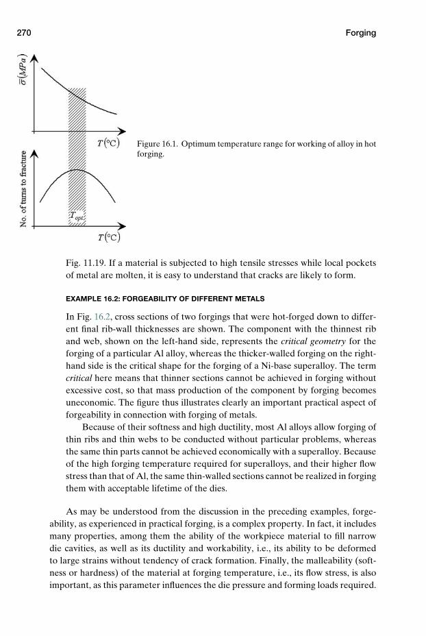
270 Forging
Figure 16.1. Optimum temperature range for working of alloy in hotforging.
Fig. 11.19. If a material is subjected to high tensile stresses while local pocketsof metal are molten, it is easy to understand that cracks are likely to form.
EXAMPLE 16.2: FORGEABILITY OF DIFFERENT METALS
In Fig. 16.2, cross sections of two forgings that were hot-forged down to differ-ent final rib-wall thicknesses are shown. The component with the thinnest riband web, shown on the left-hand side, represents the critical geometry for theforging of a particular Al alloy, whereas the thicker-walled forging on the right-hand side is the critical shape for the forging of a Ni-base superalloy. The termcritical here means that thinner sections cannot be achieved in forging withoutexcessive cost, so that mass production of the component by forging becomesuneconomic. The figure thus illustrates clearly an important practical aspect offorgeability in connection with forging of metals.
Because of their softness and high ductility, most Al alloys allow forging ofthin ribs and thin webs to be conducted without particular problems, whereasthe same thin parts cannot be achieved economically with a superalloy. Becauseof the high forging temperature required for superalloys, and their higher flowstress than that of Al, the same thin-walled sections cannot be realized in forgingthem with acceptable lifetime of the dies.
As may be understood from the discussion in the preceding examples, forge-ability, as experienced in practical forging, is a complex property. In fact, it includesmany properties, among them the ability of the workpiece material to fill narrowdie cavities, as well as its ductility and workability, i.e., its ability to be deformedto large strains without tendency of crack formation. Finally, the malleability (soft-ness or hardness) of the material at forging temperature, i.e., its flow stress, is alsoimportant, as this parameter influences the die pressure and forming loads required.
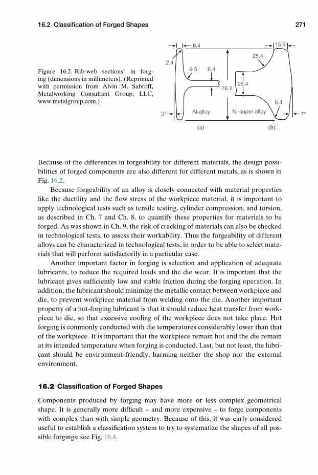
16.2 Classification of Forged Shapes 271
6.4
9.5
76.225.4
25.4
15.9
6.4
2.4
Al-alloy Ni-super alloy
6.4
3° 7°
(a) (b)
Figure 16.2. Rib-web sections1 in forg-ing (dimensions in millimeters). (Reprintedwith permission from Alvin M. Sabroff,Metalworking Consultant Group, LLC,www.metalgroup.com.)
Because of the differences in forgeability for different materials, the design possi-bilities of forged components are also different for different metals, as is shown inFig. 16.2.
Because forgeability of an alloy is closely connected with material propertieslike the ductility and the flow stress of the workpiece material, it is important toapply technological tests such as tensile testing, cylinder compression, and torsion,as described in Ch. 7 and Ch. 8, to quantify these properties for materials to beforged. As was shown in Ch. 9, the risk of cracking of materials can also be checkedin technological tests, to assess their workability. Thus the forgeability of differentalloys can be characterized in technological tests, in order to be able to select mate-rials that will perform satisfactorily in a particular case.
Another important factor in forging is selection and application of adequatelubricants, to reduce the required loads and the die wear. It is important that thelubricant gives sufficiently low and stable friction during the forging operation. Inaddition, the lubricant should minimize the metallic contact between workpiece anddie, to prevent workpiece material from welding onto the die. Another importantproperty of a hot-forging lubricant is that it should reduce heat transfer from work-piece to die, so that excessive cooling of the workpiece does not take place. Hotforging is commonly conducted with die temperatures considerably lower than thatof the workpiece. It is important that the workpiece remain hot and the die remainat its intended temperature when forging is conducted. Last, but not least, the lubri-cant should be environment-friendly, harming neither the shop nor the externalenvironment.
16.2 Classification of Forged Shapes
Components produced by forging may have more or less complex geometricalshape. It is generally more difficult – and more expensive – to forge componentswith complex than with simple geometry. Because of this, it was early considereduseful to establish a classification system to try to systematize the shapes of all pos-sible forgings; see Fig. 16.4.
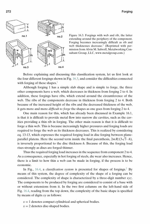
272 Forging
no.1 no.2
no.3 no.4
w/2
h h
2h 2h
w
w
t t
t Figure 16.3. Forgings with web and rib, the latterextending around the periphery of the component.Forging becomes increasingly difficult as rib andweb thicknesses decrease.1 (Reprinted with per-mission from Alvin M. Sabroff, Metalworking Con-sultant Group, LLC, www.metalgroup.com.)
Before explaining and discussing this classification system, let us first look atthe four different forgings shown in Fig. 16.3, and consider the difficulties connectedwith forging of these shapes.1
Although forging 1 has a simple slab shape and is simple to forge, the threeother components have a web, which decreases in thickness from forging 2 to 4. Inaddition, these forgings have ribs, which extend around the circumference of theweb. The ribs of the components decrease in thickness from forging 2 to 4. Bothbecause of the increased height of the ribs and the decreased thickness of the web,it gets more and more difficult to forge the shapes as one goes from forging 2 to 4.
One main reason for this, which has already been discussed in Example 16.1,is that it is difficult to provide metal flow into narrow die cavities, such as the cav-ities providing a thin rib in forging. The other main reason is that it is difficult toforge a thin web. This is because increasingly higher pressures and forging loads arerequired to forge the web as its thickness decreases. This is realized by consideringeq. 13-13, which expresses the required forging load in disc forging between plane-parallel platens. Here the second term inside the final parenthesis, 2mR/(3
√3 · h),
is inversely proportional to the disc thickness h. Because of this, the forging loadrises strongly as discs are forged thinner.
Thus the required forging load increases in the sequence from component 2 to 4.As a consequence, especially in hot forging of steels, die wear also increases. Hence,there is a limit to how thin a web can be made in forging, if the process is to beeconomic.
In Fig., 16.4, a classification system is presented for shapes of forgings.2 Bymeans of this system, the degree of complexity of the shape of a forging can beconsidered. The complexity of shape is characterized by a three-digit number xyz.The components to be produced by forging are considered to consist of a base withor without extensions from it. In the two first columns on the left-hand side ofFig. 16.4, reading from the top down, the complexity of the basic shape is specifiedby means of digits xy as follows:
x = 1 denotes compact cylindrical and spherical bodies.x = 2 denotes disc-shaped bodies.
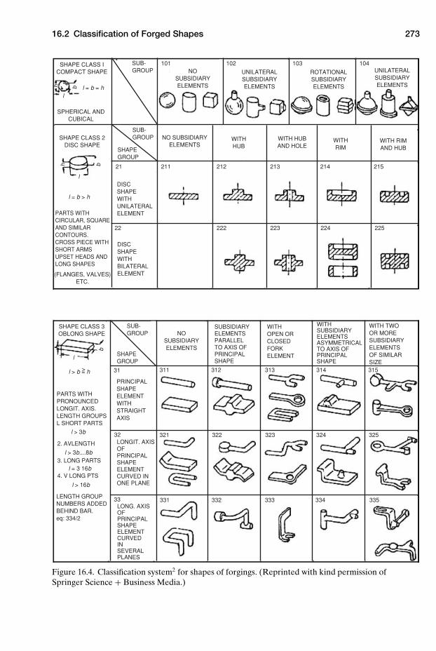
16.2 Classification of Forged Shapes 273
SHAPE CLASS I COMPACT SHAPE
SHAPE CLASS 3 OBLONG SHAPE
PARTS WITH CIRCULAR, SQUARE AND SIMILAR CONTOURS. CROSS PIECE WITH SHORT ARMS UPSET HEADS AND LONG SHAPES
PARTS WITH PRONOUNCED LONGIT. AXIS. LENGTH GROUPS L SHORT PARTS
2. AVLENGTH
3. LONG PARTS
4. V LONG PTS
LENGTH GROUP NUMBERS ADDED BEHIND BAR. eq: 334/2
LONG. AXIS OF PRINCIPAL SHAPE ELEMENT CURVED IN SEVERAL PLANES
LONGIT. AXIS OF PRINCIPAL SHAPE ELEMENT CURVED IN ONE PLANE
PRINCIPAL SHAPE ELEMENT WITH STRAIGHT AXIS
SHAPE GROUP
SUB- GROUP
SHAPE GROUP
SUB- GROUP
SUB- GROUP
DISC SHAPE WITH BILATERAL ELEMENT
DISC SHAPE WITH UNILATERAL ELEMENT
NO SUBSIDIARY ELEMENTS
NO SUBSIDIARY ELEMENTS
NO SUBSIDIARY ELEMENTS
WITH HUB
WITH RIM
WITH RIM AND HUB
WITH HUB AND HOLE
UNILATERAL SUBSIDIARY ELEMENTS
ROTATIONAL SUBSIDIARY ELEMENTS
UNILATERAL SUBSIDIARY ELEMENTS
SUBSIDIARY ELEMENTS PARALLEL TO AXIS OF PRINCIPAL SHAPE
WITH OPEN OR CLOSED FORK ELEMENT
WITH SUBSIDIARY ELEMENTS ASYMMETRICAL TO AXIS OF PRINCIPAL SHAPE
WITH TWO OR MORE SUBSIDIARY ELEMENTS OF SIMILAR SIZE
SPHERICAL AND CUBICAL
SHAPE CLASS 2 DISC SHAPE
l = b = h
l = b > h
l > b = h
l > 3b
l > 3b....8b
l = 3 16b
l > 16b
l
l
b
b
hh
l
b
h
>
101
21 211 212 213 214 215
22522422322222
31
32 321 322 323 324 325
33533433333233133
311 312 313 314 315
102 103 104
(FLANGES, VALVES) ETC.
Figure 16.4. Classification system2 for shapes of forgings. (Reprinted with kind permission ofSpringer Science + Business Media.)
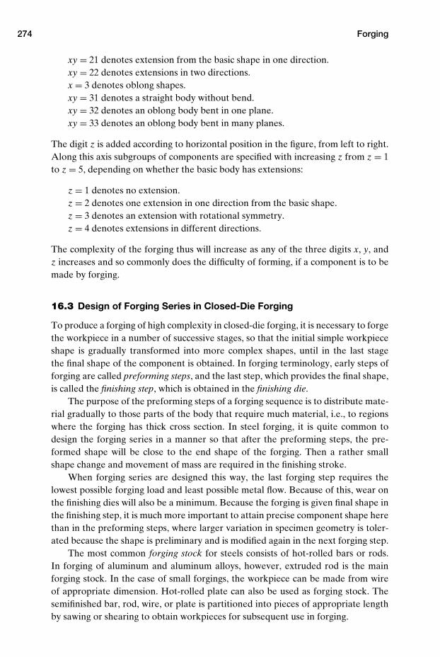
274 Forging
xy = 21 denotes extension from the basic shape in one direction.xy = 22 denotes extensions in two directions.x = 3 denotes oblong shapes.xy = 31 denotes a straight body without bend.xy = 32 denotes an oblong body bent in one plane.xy = 33 denotes an oblong body bent in many planes.
The digit z is added according to horizontal position in the figure, from left to right.Along this axis subgroups of components are specified with increasing z from z = 1to z = 5, depending on whether the basic body has extensions:
z = 1 denotes no extension.z = 2 denotes one extension in one direction from the basic shape.z = 3 denotes an extension with rotational symmetry.z = 4 denotes extensions in different directions.
The complexity of the forging thus will increase as any of the three digits x, y, andz increases and so commonly does the difficulty of forming, if a component is to bemade by forging.
16.3 Design of Forging Series in Closed-Die Forging
To produce a forging of high complexity in closed-die forging, it is necessary to forgethe workpiece in a number of successive stages, so that the initial simple workpieceshape is gradually transformed into more complex shapes, until in the last stagethe final shape of the component is obtained. In forging terminology, early steps offorging are called preforming steps, and the last step, which provides the final shape,is called the finishing step, which is obtained in the finishing die.
The purpose of the preforming steps of a forging sequence is to distribute mate-rial gradually to those parts of the body that require much material, i.e., to regionswhere the forging has thick cross section. In steel forging, it is quite common todesign the forging series in a manner so that after the preforming steps, the pre-formed shape will be close to the end shape of the forging. Then a rather smallshape change and movement of mass are required in the finishing stroke.
When forging series are designed this way, the last forging step requires thelowest possible forging load and least possible metal flow. Because of this, wear onthe finishing dies will also be a minimum. Because the forging is given final shape inthe finishing step, it is much more important to attain precise component shape herethan in the preforming steps, where larger variation in specimen geometry is toler-ated because the shape is preliminary and is modified again in the next forging step.
The most common forging stock for steels consists of hot-rolled bars or rods.In forging of aluminum and aluminum alloys, however, extruded rod is the mainforging stock. In the case of small forgings, the workpiece can be made from wireof appropriate dimension. Hot-rolled plate can also be used as forging stock. Thesemifinished bar, rod, wire, or plate is partitioned into pieces of appropriate lengthby sawing or shearing to obtain workpieces for subsequent use in forging.
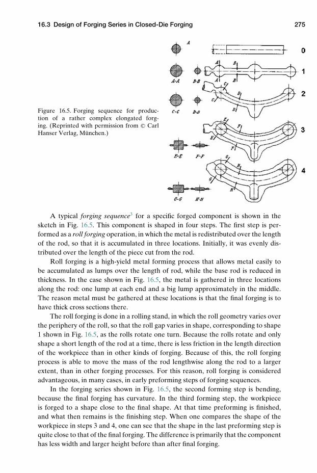
16.3 Design of Forging Series in Closed-Die Forging 275
Figure 16.5. Forging sequence for produc-tion of a rather complex elongated forg-ing. (Reprinted with permission from c© CarlHanser Verlag, Munchen.)
A typical forging sequence3 for a specific forged component is shown in thesketch in Fig. 16.5. This component is shaped in four steps. The first step is per-formed as a roll forging operation, in which the metal is redistributed over the lengthof the rod, so that it is accumulated in three locations. Initially, it was evenly dis-tributed over the length of the piece cut from the rod.
Roll forging is a high-yield metal forming process that allows metal easily tobe accumulated as lumps over the length of rod, while the base rod is reduced inthickness. In the case shown in Fig. 16.5, the metal is gathered in three locationsalong the rod: one lump at each end and a big lump approximately in the middle.The reason metal must be gathered at these locations is that the final forging is tohave thick cross sections there.
The roll forging is done in a rolling stand, in which the roll geometry varies overthe periphery of the roll, so that the roll gap varies in shape, corresponding to shape1 shown in Fig. 16.5, as the rolls rotate one turn. Because the rolls rotate and onlyshape a short length of the rod at a time, there is less friction in the length directionof the workpiece than in other kinds of forging. Because of this, the roll forgingprocess is able to move the mass of the rod lengthwise along the rod to a largerextent, than in other forging processes. For this reason, roll forging is consideredadvantageous, in many cases, in early preforming steps of forging sequences.
In the forging series shown in Fig. 16.5, the second forming step is bending,because the final forging has curvature. In the third forming step, the workpieceis forged to a shape close to the final shape. At that time preforming is finished,and what then remains is the finishing step. When one compares the shape of theworkpiece in steps 3 and 4, one can see that the shape in the last preforming step isquite close to that of the final forging. The difference is primarily that the componenthas less width and larger height before than after final forging.
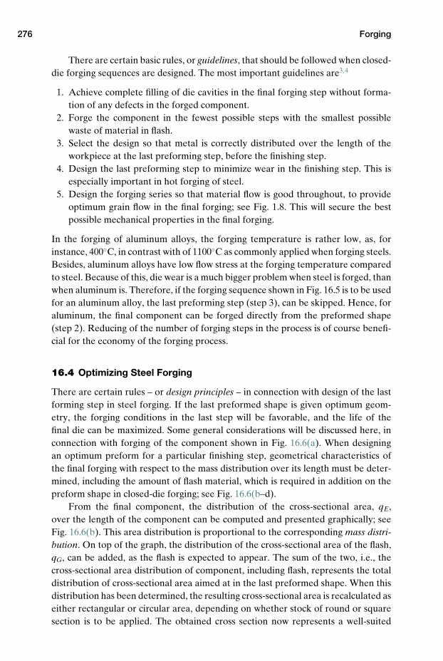
276 Forging
There are certain basic rules, or guidelines, that should be followed when closed-die forging sequences are designed. The most important guidelines are3,4
1. Achieve complete filling of die cavities in the final forging step without forma-tion of any defects in the forged component.
2. Forge the component in the fewest possible steps with the smallest possiblewaste of material in flash.
3. Select the design so that metal is correctly distributed over the length of theworkpiece at the last preforming step, before the finishing step.
4. Design the last preforming step to minimize wear in the finishing step. This isespecially important in hot forging of steel.
5. Design the forging series so that material flow is good throughout, to provideoptimum grain flow in the final forging; see Fig. 1.8. This will secure the bestpossible mechanical properties in the final forging.
In the forging of aluminum alloys, the forging temperature is rather low, as, forinstance, 400◦C, in contrast with of 1100◦C as commonly applied when forging steels.Besides, aluminum alloys have low flow stress at the forging temperature comparedto steel. Because of this, die wear is a much bigger problem when steel is forged, thanwhen aluminum is. Therefore, if the forging sequence shown in Fig. 16.5 is to be usedfor an aluminum alloy, the last preforming step (step 3), can be skipped. Hence, foraluminum, the final component can be forged directly from the preformed shape(step 2). Reducing of the number of forging steps in the process is of course benefi-cial for the economy of the forging process.
16.4 Optimizing Steel Forging
There are certain rules – or design principles – in connection with design of the lastforming step in steel forging. If the last preformed shape is given optimum geom-etry, the forging conditions in the last step will be favorable, and the life of thefinal die can be maximized. Some general considerations will be discussed here, inconnection with forging of the component shown in Fig. 16.6(a). When designingan optimum preform for a particular finishing step, geometrical characteristics ofthe final forging with respect to the mass distribution over its length must be deter-mined, including the amount of flash material, which is required in addition on thepreform shape in closed-die forging; see Fig. 16.6(b–d).
From the final component, the distribution of the cross-sectional area, qE,over the length of the component can be computed and presented graphically; seeFig. 16.6(b). This area distribution is proportional to the corresponding mass distri-bution. On top of the graph, the distribution of the cross-sectional area of the flash,qG, can be added, as the flash is expected to appear. The sum of the two, i.e., thecross-sectional area distribution of component, including flash, represents the totaldistribution of cross-sectional area aimed at in the last preformed shape. When thisdistribution has been determined, the resulting cross-sectional area is recalculated aseither rectangular or circular area, depending on whether stock of round or squaresection is to be applied. The obtained cross section now represents a well-suited
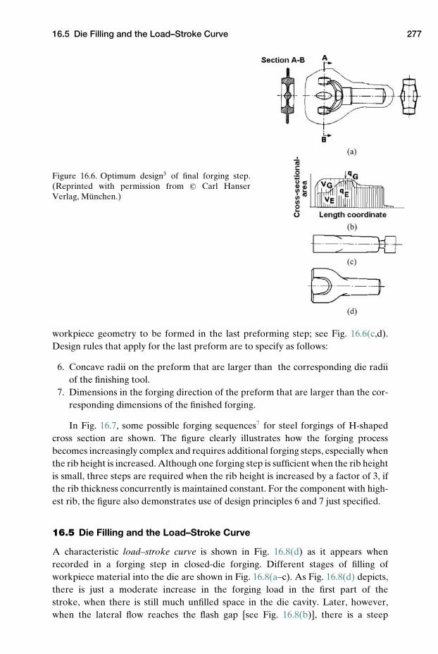
16.5 Die Filling and the Load–Stroke Curve 277
Figure 16.6. Optimum design3 of final forging step.(Reprinted with permission from c© Carl HanserVerlag, Munchen.)
workpiece geometry to be formed in the last preforming step; see Fig. 16.6(c,d).Design rules that apply for the last preform are to specify as follows:
6. Concave radii on the preform that are larger than the corresponding die radiiof the finishing tool.
7. Dimensions in the forging direction of the preform that are larger than the cor-responding dimensions of the finished forging.
In Fig. 16.7, some possible forging sequences7 for steel forgings of H-shapedcross section are shown. The figure clearly illustrates how the forging processbecomes increasingly complex and requires additional forging steps, especially whenthe rib height is increased. Although one forging step is sufficient when the rib heightis small, three steps are required when the rib height is increased by a factor of 3, ifthe rib thickness concurrently is maintained constant. For the component with high-est rib, the figure also demonstrates use of design principles 6 and 7 just specified.
16.5 Die Filling and the Load–Stroke Curve
A characteristic load–stroke curve is shown in Fig. 16.8(d) as it appears whenrecorded in a forging step in closed-die forging. Different stages of filling ofworkpiece material into the die are shown in Fig. 16.8(a–c). As Fig. 16.8(d) depicts,there is just a moderate increase in the forging load in the first part of thestroke, when there is still much unfilled space in the die cavity. Later, however,when the lateral flow reaches the flash gap [see Fig. 16.8(b)], there is a steep
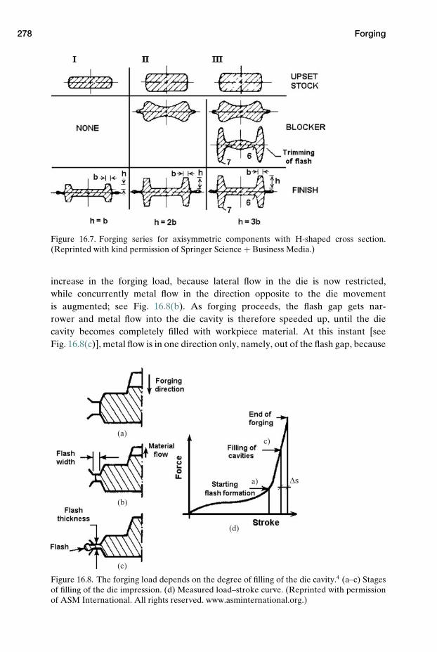
278 Forging
Figure 16.7. Forging series for axisymmetric components with H-shaped cross section.(Reprinted with kind permission of Springer Science + Business Media.)
increase in the forging load, because lateral flow in the die is now restricted,while concurrently metal flow in the direction opposite to the die movementis augmented; see Fig. 16.8(b). As forging proceeds, the flash gap gets nar-rower and metal flow into the die cavity is therefore speeded up, until the diecavity becomes completely filled with workpiece material. At this instant [seeFig. 16.8(c)], metal flow is in one direction only, namely, out of the flash gap, because
(a)
a) ∆s
(b)
(c)
c)
(d)
Figure 16.8. The forging load depends on the degree of filling of the die cavity.4 (a–c) Stagesof filling of the die impression. (d) Measured load–stroke curve. (Reprinted with permissionof ASM International. All rights reserved. www.asminternational.org.)
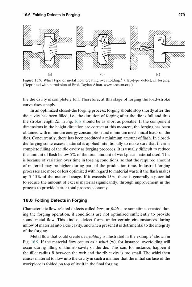
16.6 Folding Defects in Forging 279
(a) (b) (c)
Figure 16.9. Whirl type of metal flow creating over folding,5 a lap-type defect, in forging.(Reprinted with permission of Prof. Taylan Altan. www.ercnsm.org.)
the die cavity is completely full. Therefore, at this stage of forging the load–strokecurve rises steeply.
In an optimized closed-die forging process, forging should stop shortly after thedie cavity has been filled, i.e., the duration of forging after the die is full and thusthe stroke length �s in Fig. 16.8 should be as short as possible. If the componentdimensions in the height direction are correct at this moment, the forging has beenobtained with minimum energy consumption and minimum mechanical loads on thedies. Concurrently, there has been produced a minimum amount of flash. In closed-die forging some excess material is applied intentionally to make sure that there iscomplete filling of the die cavity as forging proceeds. It is usually difficult to reducethe amount of flash below 5% of the total amount of workpiece material used. Thisis because of variation over time in forging conditions, so that the required amountof material may be higher during part of the production time. Industrial forgingprocesses are more or less optimized with regard to material waste if the flash makesup 5–15% of the material usage. If it exceeds 15%, there is generally a potentialto reduce the amount of excess material significantly, through improvement in theprocess to provide better total process economy.
16.6 Folding Defects in Forging
Characteristic flow-related defects called laps, or folds, are sometimes created dur-ing the forging operation, if conditions are not optimized sufficiently to providesound metal flow. This kind of defect forms under certain circumstances duringinflow of material into a die cavity, and when present it is detrimental to the integrityof the forging.
Metal flow that could create overfolding is illustrated in the example5 shown inFig. 16.9. If the material flow occurs as a whirl (w), for instance, overfolding willoccur during filling of the rib cavity of the die. This can, for instance, happen ifthe fillet radius R between the web and the rib cavity is too small. The whirl thencauses material to flow into the cavity in such a manner that the initial surface of theworkpiece is folded on top of itself in the final forging.
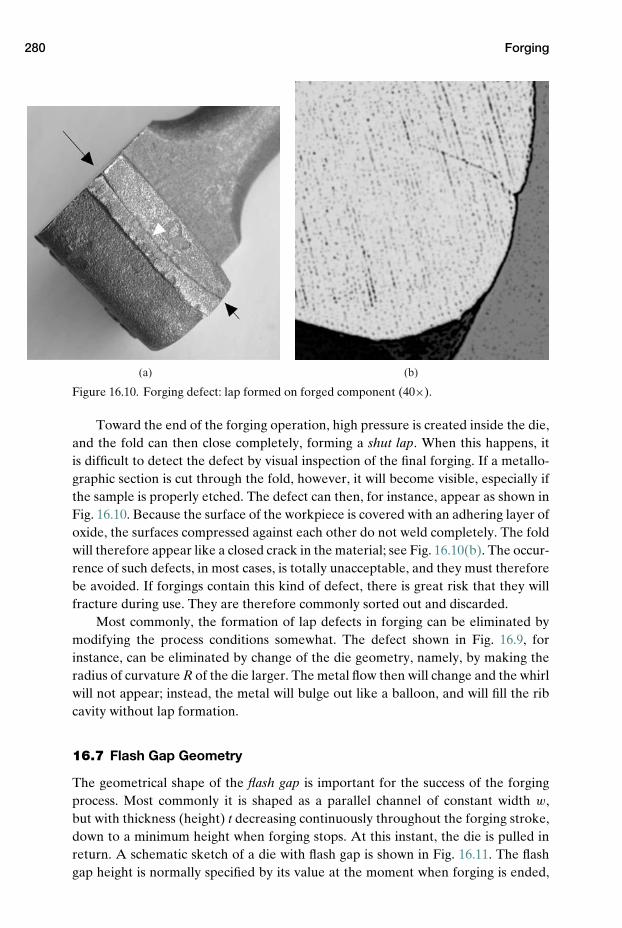
280 Forging
(a) (b)
Figure 16.10. Forging defect: lap formed on forged component (40×).
Toward the end of the forging operation, high pressure is created inside the die,and the fold can then close completely, forming a shut lap. When this happens, itis difficult to detect the defect by visual inspection of the final forging. If a metallo-graphic section is cut through the fold, however, it will become visible, especially ifthe sample is properly etched. The defect can then, for instance, appear as shown inFig. 16.10. Because the surface of the workpiece is covered with an adhering layer ofoxide, the surfaces compressed against each other do not weld completely. The foldwill therefore appear like a closed crack in the material; see Fig. 16.10(b). The occur-rence of such defects, in most cases, is totally unacceptable, and they must thereforebe avoided. If forgings contain this kind of defect, there is great risk that they willfracture during use. They are therefore commonly sorted out and discarded.
Most commonly, the formation of lap defects in forging can be eliminated bymodifying the process conditions somewhat. The defect shown in Fig. 16.9, forinstance, can be eliminated by change of the die geometry, namely, by making theradius of curvature R of the die larger. The metal flow then will change and the whirlwill not appear; instead, the metal will bulge out like a balloon, and will fill the ribcavity without lap formation.
16.7 Flash Gap Geometry
The geometrical shape of the flash gap is important for the success of the forgingprocess. Most commonly it is shaped as a parallel channel of constant width w,but with thickness (height) t decreasing continuously throughout the forging stroke,down to a minimum height when forging stops. At this instant, the die is pulled inreturn. A schematic sketch of a die with flash gap is shown in Fig. 16.11. The flashgap height is normally specified by its value at the moment when forging is ended,
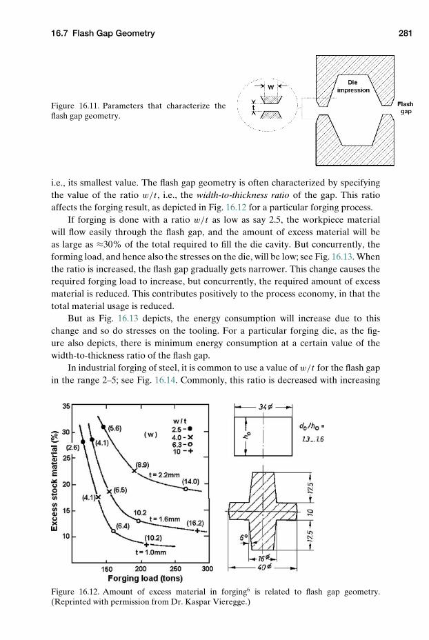
16.7 Flash Gap Geometry 281
Figure 16.11. Parameters that characterize theflash gap geometry.
i.e., its smallest value. The flash gap geometry is often characterized by specifyingthe value of the ratio w/t , i.e., the width-to-thickness ratio of the gap. This ratioaffects the forging result, as depicted in Fig. 16.12 for a particular forging process.
If forging is done with a ratio w/t as low as say 2.5, the workpiece materialwill flow easily through the flash gap, and the amount of excess material will beas large as ≈30% of the total required to fill the die cavity. But concurrently, theforming load, and hence also the stresses on the die, will be low; see Fig. 16.13. Whenthe ratio is increased, the flash gap gradually gets narrower. This change causes therequired forging load to increase, but concurrently, the required amount of excessmaterial is reduced. This contributes positively to the process economy, in that thetotal material usage is reduced.
But as Fig. 16.13 depicts, the energy consumption will increase due to thischange and so do stresses on the tooling. For a particular forging die, as the fig-ure also depicts, there is minimum energy consumption at a certain value of thewidth-to-thickness ratio of the flash gap.
In industrial forging of steel, it is common to use a value of w/t for the flash gapin the range 2–5; see Fig. 16.14. Commonly, this ratio is decreased with increasing
Figure 16.12. Amount of excess material in forging6 is related to flash gap geometry.(Reprinted with permission from Dr. Kaspar Vieregge.)
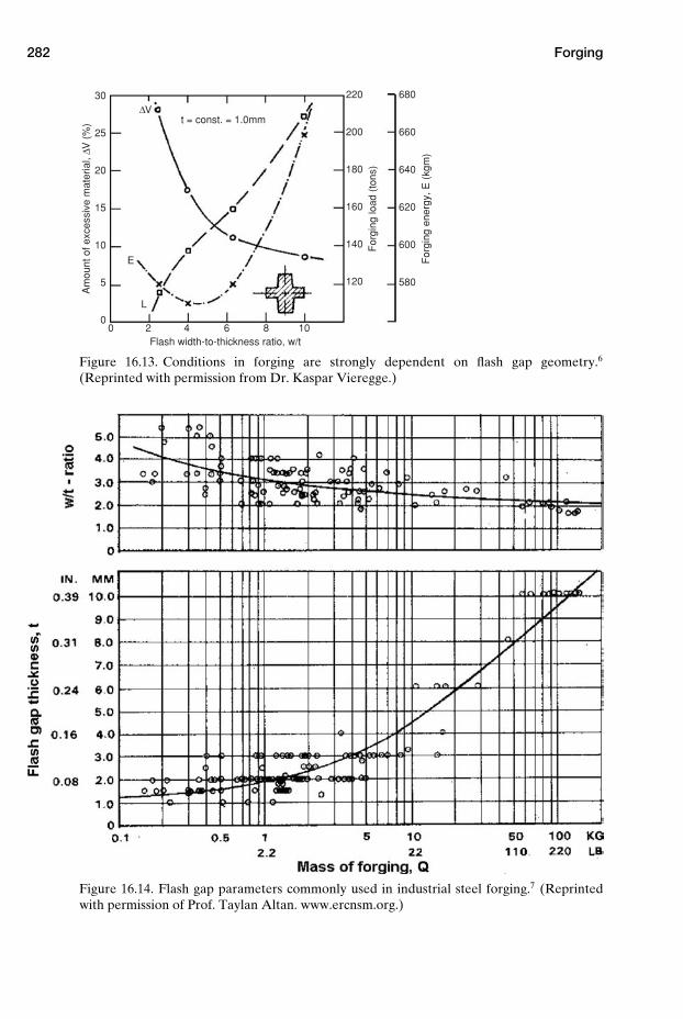
282 Forging
30
25
20
15
10
5
0
220
200
180
160
140
120
680
660
640
620
600
580
For
ging
load
(to
ns)
Am
ount
of e
xces
sive
mat
eria
l, ∆V
(%
)
For
ging
ene
rgy,
E (
kgm
)
Flash width-to-thickness ratio, w/t
t = const. = 1.0mm
0 2 4 6 8 10
E
L
∆V
Figure 16.13. Conditions in forging are strongly dependent on flash gap geometry.6
(Reprinted with permission from Dr. Kaspar Vieregge.)
Figure 16.14. Flash gap parameters commonly used in industrial steel forging.7 (Reprintedwith permission of Prof. Taylan Altan. www.ercnsm.org.)
Notes 283
weight of the forging. When the width-to-thickness ratio of the flash gap exceeds 5,the stresses on the die become large. Concurrently, the die lifetime is significantlyreduced, so in industrial forging, such high ratios are not commonly used.
Problems
16.1 Commonly used forging processes are divided in two subgroups.
(a) Mention the name of each subgroup. Describe the main differencesbetween them.
(b) Sketch a typical load–stroke curve as it is measured in forging. Partition thecurve into separate regions in which different flow phenomena take placeinside the die cavity. Describe briefly what characterizes metal flow in eachregion.
(c) What characterizes the state of plane strain deformation? Explain towhat extent it can be realized in a laboratory process and in industrialforging.
(d) Describe what is meant by the term axisymmetric deformation.
In compression of metal between two plane-parallel dies, the necessary formingload and the friction hill (i.e., the pressure distribution) depend on the nature of thecompression process, i.e., whether it is axisymmetric or is in plane strain.
(e) Specify the expressions for forming load and pressure distribution for eachkind of compression process, as they are determined by the slab method.Compare the expressions for each of the deformation processes. What isthe difference between the two?
16.2 In technological literature, good workability of a workpiece material some-times is claimed to require the following:
(i) The material should have low deformation resistance.(ii) The material should deform plastically without formation of internal or sur-
face cracks.
Comment on the goodness of the formability definition used in this case. Try to givea better definition.
NOTES
1. Sabroff, A. M., Boulger, F. W., and Henning, H. H.: “Forging Materials and Practices,”Reinholdt, New York, 1968.
2. Spies, K.: “Preforming in Forging and the Preparation of Reducer Rolling,” doctoralthesis, Technical University Hannover, 1959.
3. Haller, H. W.: “Handbook of Forging” (in German), Carl Hanser Verlag, Munchen,1971.
4. Altan, T., Oh, S.-I., and Gegel, H. L. (Eds.): “Metal Forming, Fundamentals and Appli-cations,” ASM Int., 1983, pp. 143–170.
5. Subramanian, T. L., Akgerman, K., and Altan, T.: “Application of computer-aideddesign and manufacturing to precision isothermal forging of titanium alloys,” Batelle’s

284 Forging
Columbus Laboratories, Final report AML-TR-77-108, Vols. I, II and III. Air ForceMaterials Lab., July, 1977.
6. Vieregge, K.: “Ein Beitrag zur Gestaltung des Gratspaltes beim Gesenkschmieden,” Dis-sertation, Technical University of Hannover, 1969 (in German).
7. Lange, K., and Meyer-Nolkemper, H.: “Closed-Die Forging” (in German), Springer-Verlag, Berlin, 1977.
REFERENCES
Altan, T., Oh, S.-I., and Gegel, H. L. (Eds.): “Metal Forming, Fundamentals and Applica-tions,” ASM Int., 1983, pp. 143–170.
Altan, T., Ngaile, G., and Shen, G.: “Cold and Hot Forging: Fundamentals and Applications,”ASM Int., Materials Park, Ohio, 2004.
Altan, T.: “Hot forging: Trends and applications,” fourth Precision Forging Workshop,Plymouth, Michigan, 2008.
Byrer, T., Semiatin, S. L., and Vollmer, D. C.: “Forging Handbook,” ASM Int., Metals Park,Ohio, 1985, pp. 112–114.
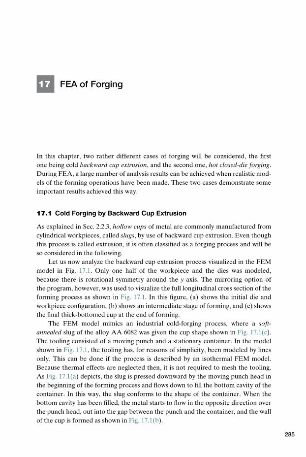
17 FEA of Forging
In this chapter, two rather different cases of forging will be considered, the firstone being cold backward cup extrusion, and the second one, hot closed-die forging.During FEA, a large number of analysis results can be achieved when realistic mod-els of the forming operations have been made. These two cases demonstrate someimportant results achieved this way.
17.1 Cold Forging by Backward Cup Extrusion
As explained in Sec. 2.2.3, hollow cups of metal are commonly manufactured fromcylindrical workpieces, called slugs, by use of backward cup extrusion. Even thoughthis process is called extrusion, it is often classified as a forging process and will beso considered in the following.
Let us now analyze the backward cup extrusion process visualized in the FEMmodel in Fig. 17.1. Only one half of the workpiece and the dies was modeled,because there is rotational symmetry around the y-axis. The mirroring option ofthe program, however, was used to visualize the full longitudinal cross section of theforming process as shown in Fig. 17.1. In this figure, (a) shows the initial die andworkpiece configuration, (b) shows an intermediate stage of forming, and (c) showsthe final thick-bottomed cup at the end of forming.
The FEM model mimics an industrial cold-forging process, where a soft-annealed slug of the alloy AA 6082 was given the cup shape shown in Fig. 17.1(c).The tooling consisted of a moving punch and a stationary container. In the modelshown in Fig. 17.1, the tooling has, for reasons of simplicity, been modeled by linesonly. This can be done if the process is described by an isothermal FEM model.Because thermal effects are neglected then, it is not required to mesh the tooling.As Fig. 17.1(a) depicts, the slug is pressed downward by the moving punch head inthe beginning of the forming process and flows down to fill the bottom cavity of thecontainer. In this way, the slug conforms to the shape of the container. When thebottom cavity has been filled, the metal starts to flow in the opposite direction overthe punch head, out into the gap between the punch and the container, and the wallof the cup is formed as shown in Fig. 17.1(b).
285
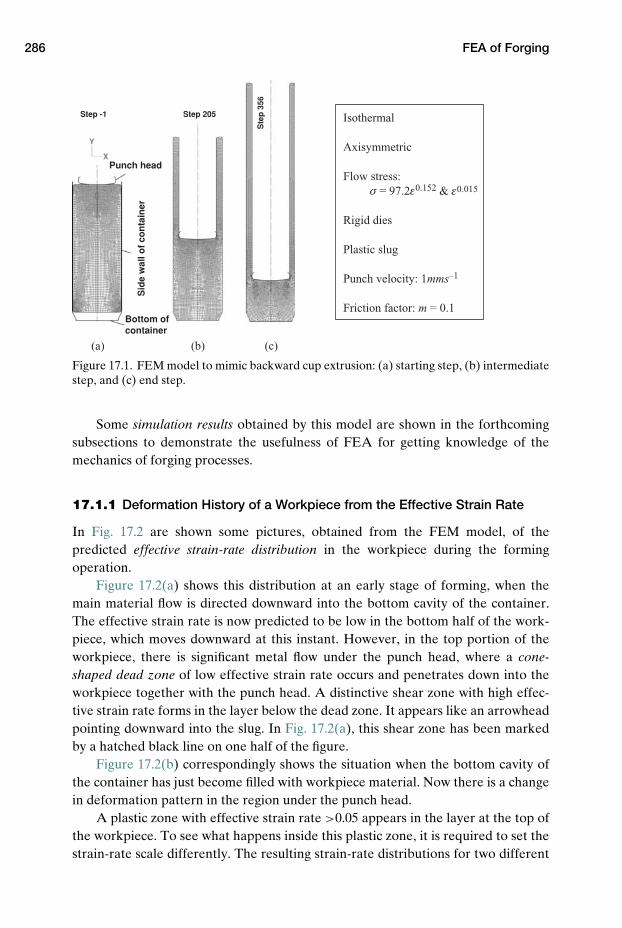
286 FEA of Forging
Step 205
Ste
p 3
56
Step -1
X
Y
(a) (b) (c)
Punch head
Sid
e w
all o
f co
nta
iner
Bottom of container
Isothermal
Axisymmetric
Flow stress: σ = 97.2ε0.152 & ε0.015
Rigid dies
Plastic slug
Punch velocity: 1mms–1
Friction factor: m = 0.1
Figure 17.1. FEM model to mimic backward cup extrusion: (a) starting step, (b) intermediatestep, and (c) end step.
Some simulation results obtained by this model are shown in the forthcomingsubsections to demonstrate the usefulness of FEA for getting knowledge of themechanics of forging processes.
17.1.1 Deformation History of a Workpiece from the Effective Strain Rate
In Fig. 17.2 are shown some pictures, obtained from the FEM model, of thepredicted effective strain-rate distribution in the workpiece during the formingoperation.
Figure 17.2(a) shows this distribution at an early stage of forming, when themain material flow is directed downward into the bottom cavity of the container.The effective strain rate is now predicted to be low in the bottom half of the work-piece, which moves downward at this instant. However, in the top portion of theworkpiece, there is significant metal flow under the punch head, where a cone-shaped dead zone of low effective strain rate occurs and penetrates down into theworkpiece together with the punch head. A distinctive shear zone with high effec-tive strain rate forms in the layer below the dead zone. It appears like an arrowheadpointing downward into the slug. In Fig. 17.2(a), this shear zone has been markedby a hatched black line on one half of the figure.
Figure 17.2(b) correspondingly shows the situation when the bottom cavity ofthe container has just become filled with workpiece material. Now there is a changein deformation pattern in the region under the punch head.
A plastic zone with effective strain rate >0.05 appears in the layer at the top ofthe workpiece. To see what happens inside this plastic zone, it is required to set thestrain-rate scale differently. The resulting strain-rate distributions for two different
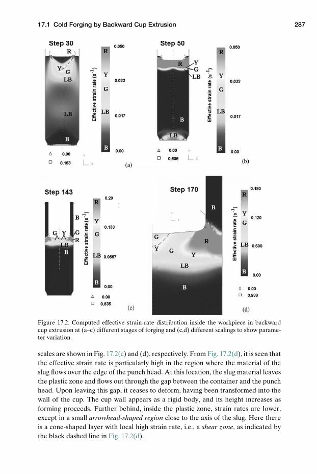
17.1 Cold Forging by Backward Cup Extrusion 287
Figure 17.2. Computed effective strain-rate distribution inside the workpiece in backwardcup extrusion at (a–c) different stages of forging and (c,d) different scalings to show parame-ter variation.
scales are shown in Fig. 17.2(c) and (d), respectively. From Fig. 17.2(d), it is seen thatthe effective strain rate is particularly high in the region where the material of theslug flows over the edge of the punch head. At this location, the slug material leavesthe plastic zone and flows out through the gap between the container and the punchhead. Upon leaving this gap, it ceases to deform, having been transformed into thewall of the cup. The cup wall appears as a rigid body, and its height increases asforming proceeds. Further behind, inside the plastic zone, strain rates are lower,except in a small arrowhead-shaped region close to the axis of the slug. Here thereis a cone-shaped layer with local high strain rate, i.e., a shear zone, as indicated bythe black dashed line in Fig. 17.2(d).
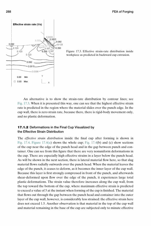
288 FEA of Forging
Figure 17.3. Effective strain-rate distribution insideworkpiece as predicted in backward cup extrusion.
An alternative is to show the strain-rate distribution by contour lines; seeFig. 17.3. When it is presented this way, one can see that the highest effective strainrate is predicted in the region where the material slides over the punch edge. In thecup wall, there is zero strain rate, because there, there is rigid-body movement only,and no plastic deformation.
17.1.2 Deformations in the Final Cup Visualized bythe Effective Strain Distribution
The effective strain distribution inside the final cup after forming is shown inFig. 17.4. Figure 17.4(a) shows the whole cup; Fig. 17.4(b) and (c) show sectionsof the cup near the edge of the punch head and in the gap between punch and con-tainer. One can see from this figure that there are very nonuniform deformations inthe cup. There are especially high effective strains in a layer below the punch head.As will be shown in the next section, there is lateral material flow here, so that slugmaterial flows radially outwards over the punch head. When the material leaves theedge of the punch, it ceases to deform, as it becomes the inner layer of the cup wall.Because this layer is first strongly compressed in front of the punch, and afterwardsshear-deformed upon flow over the edge of the punch, it experiences large totalplastic deformations. The strain value therefore increases along the cup wall, fromthe top toward the bottom of the cup, where maximum effective strain is predictedto exceed a value of 5 at the instant when forming of the cup is finished. The materialthat flows out through the gap between the punch head and container into the outerlayer of the cup wall, however, is considerably less strained: the effective strain heredoes not exceed 1.5. Another observation is that material in the top of the cup walland material remaining in the base of the cup are subjected only to minute effective
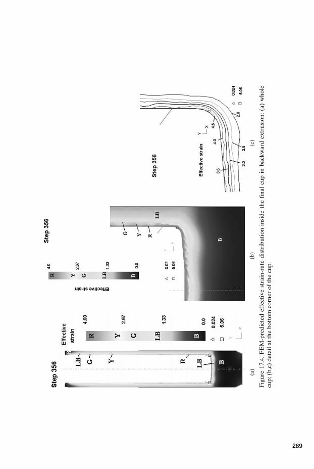
(a)
(b)
(c)
Fig
ure
17.4
.F
EM
-pre
dict
edef
fect
ive
stra
in-r
ate
dist
ribu
tion
insi
deth
efin
alcu
pin
back
war
dex
trus
ion:
(a)
who
lecu
p;(b
,c)
deta
ilat
the
bott
omco
rner
ofth
ecu
p.
289
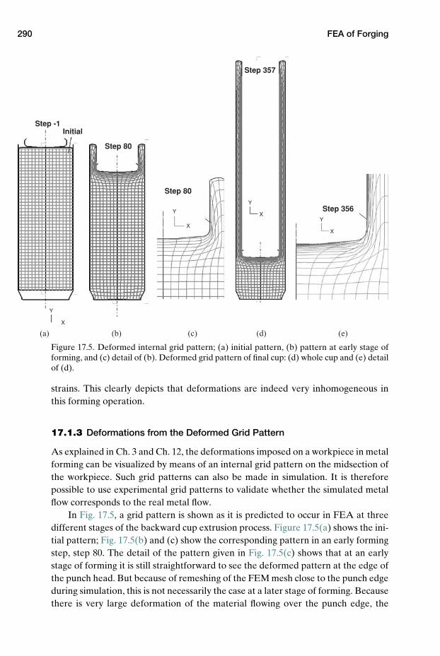
290 FEA of Forging
Step -1
Step 80
Step 80
Step 357
Step 356
Initial
X
X
X
X
Y
Y
Y
Y
(a) (b) (c) (d) (e)
Figure 17.5. Deformed internal grid pattern; (a) initial pattern, (b) pattern at early stage offorming, and (c) detail of (b). Deformed grid pattern of final cup: (d) whole cup and (e) detailof (d).
strains. This clearly depicts that deformations are indeed very inhomogeneous inthis forming operation.
17.1.3 Deformations from the Deformed Grid Pattern
As explained in Ch. 3 and Ch. 12, the deformations imposed on a workpiece in metalforming can be visualized by means of an internal grid pattern on the midsection ofthe workpiece. Such grid patterns can also be made in simulation. It is thereforepossible to use experimental grid patterns to validate whether the simulated metalflow corresponds to the real metal flow.
In Fig. 17.5, a grid pattern is shown as it is predicted to occur in FEA at threedifferent stages of the backward cup extrusion process. Figure 17.5(a) shows the ini-tial pattern; Fig. 17.5(b) and (c) show the corresponding pattern in an early formingstep, step 80. The detail of the pattern given in Fig. 17.5(c) shows that at an earlystage of forming it is still straightforward to see the deformed pattern at the edge ofthe punch head. But because of remeshing of the FEM mesh close to the punch edgeduring simulation, this is not necessarily the case at a later stage of forming. Becausethere is very large deformation of the material flowing over the punch edge, the
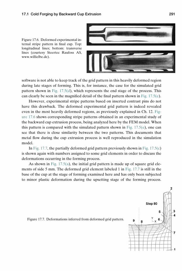
17.1 Cold Forging by Backward Cup Extrusion 291
Figure 17.6. Deformed experimental in-ternal stripe pattern in final cup. Top:longitudinal lines; bottom: transverselines (courtesy Steertec Raufoss AS,www.willielbe.de).
software is not able to keep track of the grid pattern in this heavily deformed regionduring late stages of forming. This is, for instance, the case for the simulated gridpattern shown in Fig. 17.5(d), which represents the end stage of the process. Thiscan clearly be seen in the magnified detail of the final pattern shown in Fig. 17.5(e).
However, experimental stripe patterns based on inserted contrast pins do nothave this drawback. The deformed experimental grid pattern is indeed revealedeven in the most heavily deformed regions, as previously explained in Ch. 12. Fig-ure 17.6 shows corresponding stripe patterns obtained in an experimental study ofthe backward cup extrusion process, being analyzed here by the FEM model. Whenthis pattern is compared with the simulated pattern shown in Fig. 17.5(e), one cansee that there is close similarity between the two patterns. This documents thatmetal flow during the cup extrusion process is well reproduced in the simulationmodel.
In Fig. 17.7, the partially deformed grid pattern previously shown in Fig. 17.5(c)is shown again with numbers assigned to some grid elements in order to discuss thedeformations occurring in the forming process.
As shown in Fig. 17.5(a), the initial grid pattern is made up of square grid ele-ments of side 5 mm. The deformed grid element labeled 1 in Fig. 17.7 is still in thebase of the cup at the stage of forming examined here and has only been subjectedto minor plastic deformation during the upsetting stage of the forming process.
Figure 17.7. Deformations inferred from deformed grid pattern.
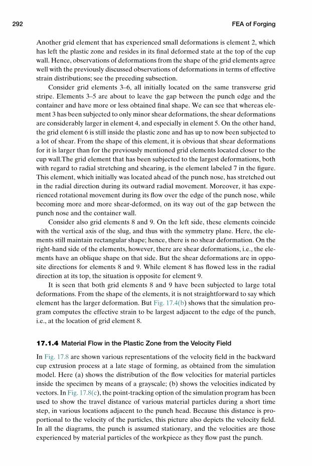
292 FEA of Forging
Another grid element that has experienced small deformations is element 2, whichhas left the plastic zone and resides in its final deformed state at the top of the cupwall. Hence, observations of deformations from the shape of the grid elements agreewell with the previously discussed observations of deformations in terms of effectivestrain distributions; see the preceding subsection.
Consider grid elements 3–6, all initially located on the same transverse gridstripe. Elements 3–5 are about to leave the gap between the punch edge and thecontainer and have more or less obtained final shape. We can see that whereas ele-ment 3 has been subjected to only minor shear deformations, the shear deformationsare considerably larger in element 4, and especially in element 5. On the other hand,the grid element 6 is still inside the plastic zone and has up to now been subjected toa lot of shear. From the shape of this element, it is obvious that shear deformationsfor it is larger than for the previously mentioned grid elements located closer to thecup wall.The grid element that has been subjected to the largest deformations, bothwith regard to radial stretching and shearing, is the element labeled 7 in the figure.This element, which initially was located ahead of the punch nose, has stretched outin the radial direction during its outward radial movement. Moreover, it has expe-rienced rotational movement during its flow over the edge of the punch nose, whilebecoming more and more shear-deformed, on its way out of the gap between thepunch nose and the container wall.
Consider also grid elements 8 and 9. On the left side, these elements coincidewith the vertical axis of the slug, and thus with the symmetry plane. Here, the ele-ments still maintain rectangular shape; hence, there is no shear deformation. On theright-hand side of the elements, however, there are shear deformations, i.e., the ele-ments have an oblique shape on that side. But the shear deformations are in oppo-site directions for elements 8 and 9. While element 8 has flowed less in the radialdirection at its top, the situation is opposite for element 9.
It is seen that both grid elements 8 and 9 have been subjected to large totaldeformations. From the shape of the elements, it is not straightforward to say whichelement has the larger deformation. But Fig. 17.4(b) shows that the simulation pro-gram computes the effective strain to be largest adjacent to the edge of the punch,i.e., at the location of grid element 8.
17.1.4 Material Flow in the Plastic Zone from the Velocity Field
In Fig. 17.8 are shown various representations of the velocity field in the backwardcup extrusion process at a late stage of forming, as obtained from the simulationmodel. Here (a) shows the distribution of the flow velocities for material particlesinside the specimen by means of a grayscale; (b) shows the velocities indicated byvectors. In Fig. 17.8(c), the point-tracking option of the simulation program has beenused to show the travel distance of various material particles during a short timestep, in various locations adjacent to the punch head. Because this distance is pro-portional to the velocity of the particles, this picture also depicts the velocity field.In all the diagrams, the punch is assumed stationary, and the velocities are thoseexperienced by material particles of the workpiece as they flow past the punch.
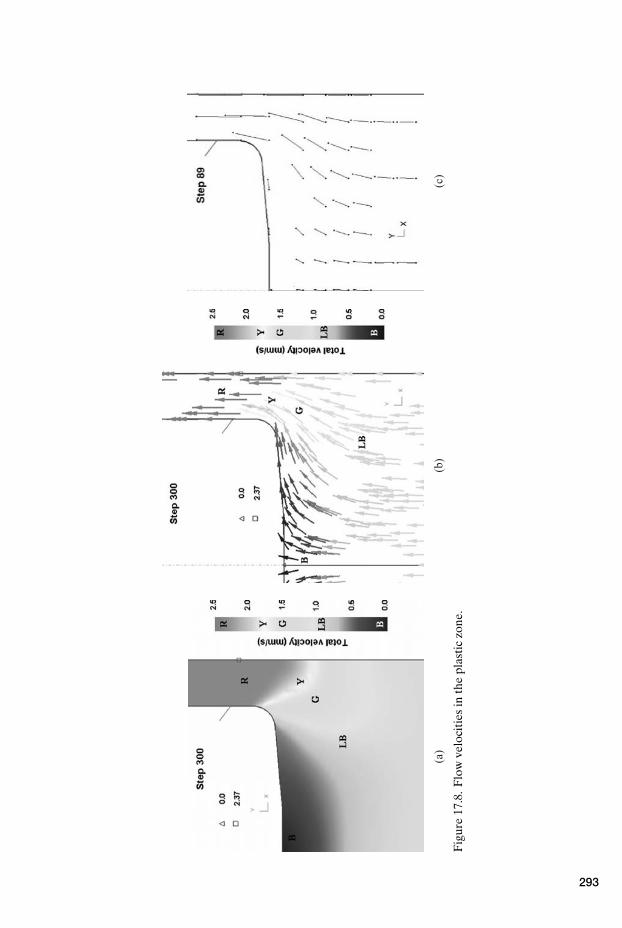
(a)
(b)
(c)
Fig
ure
17.8
.F
low
velo
citi
esin
the
plas
tic
zone
.
293
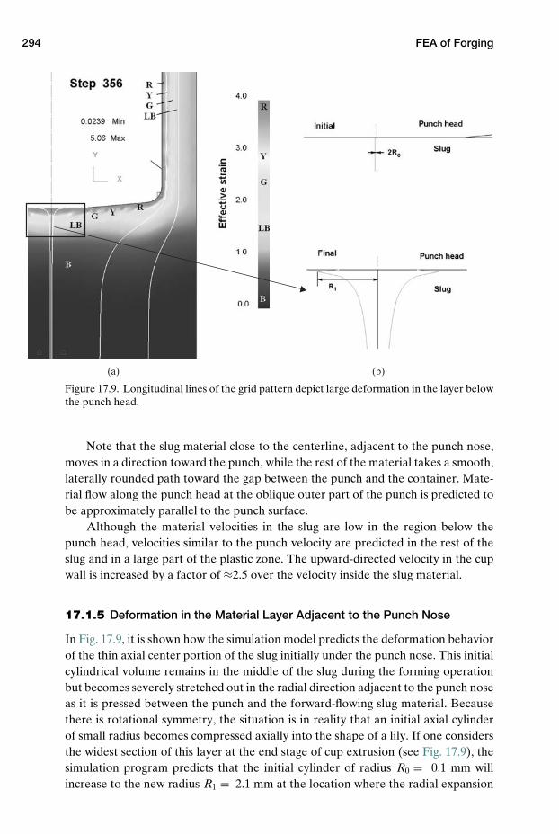
294 FEA of Forging
(a) (b)
Figure 17.9. Longitudinal lines of the grid pattern depict large deformation in the layer belowthe punch head.
Note that the slug material close to the centerline, adjacent to the punch nose,moves in a direction toward the punch, while the rest of the material takes a smooth,laterally rounded path toward the gap between the punch and the container. Mate-rial flow along the punch head at the oblique outer part of the punch is predicted tobe approximately parallel to the punch surface.
Although the material velocities in the slug are low in the region below thepunch head, velocities similar to the punch velocity are predicted in the rest of theslug and in a large part of the plastic zone. The upward-directed velocity in the cupwall is increased by a factor of ≈2.5 over the velocity inside the slug material.
17.1.5 Deformation in the Material Layer Adjacent to the Punch Nose
In Fig. 17.9, it is shown how the simulation model predicts the deformation behaviorof the thin axial center portion of the slug initially under the punch nose. This initialcylindrical volume remains in the middle of the slug during the forming operationbut becomes severely stretched out in the radial direction adjacent to the punch noseas it is pressed between the punch and the forward-flowing slug material. Becausethere is rotational symmetry, the situation is in reality that an initial axial cylinderof small radius becomes compressed axially into the shape of a lily. If one considersthe widest section of this layer at the end stage of cup extrusion (see Fig. 17.9), thesimulation program predicts that the initial cylinder of radius R0 = 0.1 mm willincrease to the new radius R1 = 2.1 mm at the location where the radial expansion
17.1 Cold Forging by Backward Cup Extrusion 295
is largest. A simple approximate calculation of the effective strain thus yields thefollowing result for the widest section of the lily:
ε = lnA1
A0= ln
πR21
πR20
= ln2.12
0.12= 6.1
This value can be compared with the corresponding maximum effective strain valuecomputed by the simulation model. As shown in Fig. 17.4, the maximum effectivestrain value predicted by the simulation model is 5.06. This strain is predicted tooccur in the subsurface layer of the cup, adjacent to the edge of the punch head,at the end of forming, and it is denoted by a small square in Fig. 17.9. This showsthat it is not straightforward by FEA to compute the net deformation in the heavilydeforming subsurface layer of the workpiece, located in front of the punch noseduring forming. The reason for this is that there are in reality large gradients ofdeformation in this layer.
17.1.6 Emptying Diagram
Emptying diagrams were made by the simulation model for the backward cup extru-sion process and are shown in Fig. 17.10. They correspond to the emptying dia-grams that were made manually on the basis of deformed experimental grid patternsobtained in the forward extrusion processes; see Ch. 12.
An emptying diagram is easily obtained by means of the FEM model. The sim-ulation is run to the end stage of forming, as shown in Fig. 17.10(a) and (c); then a“grid pattern” consisting of one single transverse (T) line is added into the sectionof the workpiece, as shown by line A–A in Fig. 17.10(a).
This T-line then represents the boundary line between the material in the cupwall and the material in the base of the cup after the end of extrusion. The simulationmodel was run backwards to the initial state to show where material particles alongthis line were placed at the start of forming; see Fig. 17.10(b). Because the FEMprogram remeshes the FEM grid many times during the course of simulation, thesimulation program is not able to keep track of those material points that flow closeto the punch edge when the backward point tracking is done. Because of this, onlypart of the line gets tracked back to the initial location in the slug.
Because we know from the discussion in connection with Fig. 17.9 that the mid-dle of the slug remains unextruded (i.e., inside the base of the final cup), one canmanually extrapolate the transverse emptying line upwards toward the punch head.This was done by drawing the thin black lines shown in Fig. 17.10(b). From theresulting figure, the location of the slug material that forms the cup wall can beidentified and distinguished from the material that forms the base.
A pattern consisting of multiple horizontal lines has correspondingly beenadded to the section of the final component in Fig. 17.10(c). Figure 17.10(d) showsthe resulting emptying diagram when all these lines are traced back to the initialstate. From this diagram, we can now clearly see from where inside the slug the topslice of the cup wall, the slice below the top slice, etc., originate.
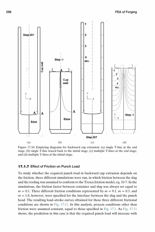
296 FEA of Forging
(a) (b) (c) (d)
Figure 17.10. Emptying diagrams for backward cup extrusion: (a) single T-line at the endstage, (b) single T-line traced back to the initial stage, (c) multiple T-lines at the end stage,and (d) multiple T-lines at the initial stage.
17.1.7 Effect of Friction on Punch Load
To study whether the required punch load in backward cup extrusion depends onthe friction, three different simulations were run, in which friction between the slugand the tooling was assumed to conform to the Tresca friction model, eq. 10-7. In thesimulations, the friction factor between container and slug was always set equal tom = 0.1. Three different friction conditions represented by m = 0.1, m = 0.3, andm = 1.0, however, were specified for the interface between the slug and the punchhead. The resulting load–stroke curves obtained for these three different frictionalconditions are shown in Fig. 17.11. In this analysis, process conditions other thanfriction were assumed constant, equal to those specified in Fig. 17.1. As Fig. 17.11shows, the prediction in this case is that the required punch load will increase with
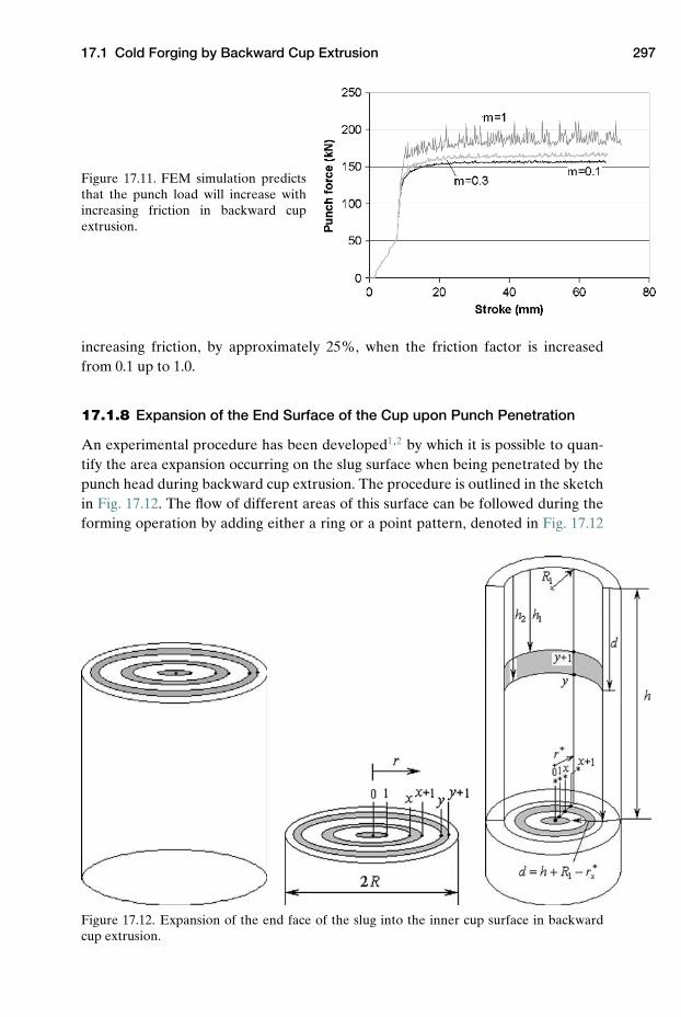
17.1 Cold Forging by Backward Cup Extrusion 297
Figure 17.11. FEM simulation predictsthat the punch load will increase withincreasing friction in backward cupextrusion.
increasing friction, by approximately 25%, when the friction factor is increasedfrom 0.1 up to 1.0.
17.1.8 Expansion of the End Surface of the Cup upon Punch Penetration
An experimental procedure has been developed1,2 by which it is possible to quan-tify the area expansion occurring on the slug surface when being penetrated by thepunch head during backward cup extrusion. The procedure is outlined in the sketchin Fig. 17.12. The flow of different areas of this surface can be followed during theforming operation by adding either a ring or a point pattern, denoted in Fig. 17.12
Figure 17.12. Expansion of the end face of the slug into the inner cup surface in backwardcup extrusion.
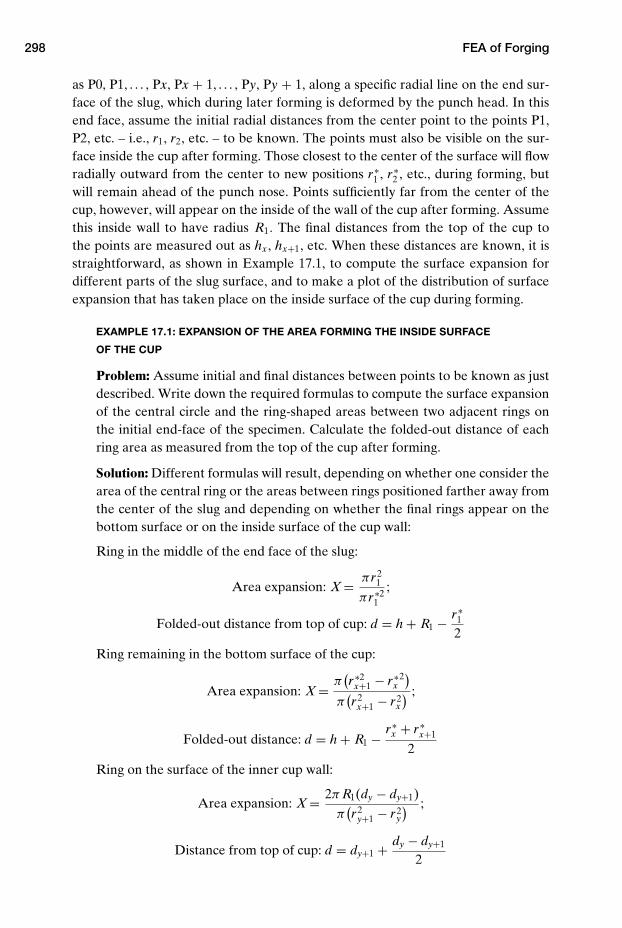
298 FEA of Forging
as P0, P1, . . . , Px, Px + 1, . . . , Py, Py + 1, along a specific radial line on the end sur-face of the slug, which during later forming is deformed by the punch head. In thisend face, assume the initial radial distances from the center point to the points P1,P2, etc. – i.e., r1, r2, etc. – to be known. The points must also be visible on the sur-face inside the cup after forming. Those closest to the center of the surface will flowradially outward from the center to new positions r∗
1 , r∗2 , etc., during forming, but
will remain ahead of the punch nose. Points sufficiently far from the center of thecup, however, will appear on the inside of the wall of the cup after forming. Assumethis inside wall to have radius R1. The final distances from the top of the cup tothe points are measured out as hx, hx+1, etc. When these distances are known, it isstraightforward, as shown in Example 17.1, to compute the surface expansion fordifferent parts of the slug surface, and to make a plot of the distribution of surfaceexpansion that has taken place on the inside surface of the cup during forming.
EXAMPLE 17.1: EXPANSION OF THE AREA FORMING THE INSIDE SURFACE
OF THE CUP
Problem: Assume initial and final distances between points to be known as justdescribed. Write down the required formulas to compute the surface expansionof the central circle and the ring-shaped areas between two adjacent rings onthe initial end-face of the specimen. Calculate the folded-out distance of eachring area as measured from the top of the cup after forming.
Solution: Different formulas will result, depending on whether one consider thearea of the central ring or the areas between rings positioned farther away fromthe center of the slug and depending on whether the final rings appear on thebottom surface or on the inside surface of the cup wall:
Ring in the middle of the end face of the slug:
Area expansion: X = πr21
πr∗21
;
Folded-out distance from top of cup: d = h + R1 − r∗1
2
Ring remaining in the bottom surface of the cup:
Area expansion: X = π(r∗2
x+1 − r∗x
2)π
(r2
x+1 − r2x
) ;
Folded-out distance: d = h + R1 − r∗x + r∗
x+1
2
Ring on the surface of the inner cup wall:
Area expansion: X = 2π R1(dy − dy+1)
π(r2
y+1 − r2y
) ;
Distance from top of cup: d = dy+1 + dy − dy+1
2
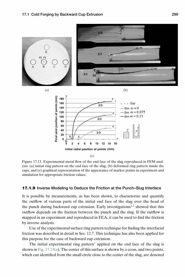
17.1 Cold Forging by Backward Cup Extrusion 299
(a) (b)
(c)
Figure 17.13. Experimental metal flow of the end face of the slug reproduced in FEM anal-ysis: (a) initial ring pattern on the end face of the slug, (b) deformed ring pattern inside thecups, and (c) graphical representation of the appearance of marker points in experiment andsimulation for appropriate friction values.
17.1.9 Inverse Modeling to Deduce the Friction at the Punch–Slug Interface
It is possible by measurements, as has been shown, to characterize and quantifythe outflow of various parts of the initial end face of the slug over the head ofthe punch during backward cup extrusion. Early investigations1,2 showed that thisoutflow depends on the friction between the punch and the slug. If the outflow ismapped in an experiment and reproduced in FEA, it can be used to find the frictionby inverse analysis.
Use of the experimental surface ring pattern technique for finding the interfacialfriction was described in detail in Sec. 12.7. This technique has also been applied forthis purpose for the case of backward cup extrusion.
The initial experimental ring pattern3 applied on the end face of the slug isshown in Fig. 17.13(a). The center of this surface is shown by a cross, and two points,which can identified from the small circle close to the center of the slug, are denoted

300 FEA of Forging
P1 and P2. The pattern of the small circles inside the cup at three different stages offorming is shown in Fig. 17.13(b). The points P1 and P2 as they appear after formingare easily identified. The other marker circles – the closest (C), the middle (A), andthe farthest (D) away from the center of the slug – define additional points on thissurface, which can be applied for surface expansion analysis.
When the initial and final distances defined by all the small circles on the surfaceto be analyzed have been measured, the best way of depicting the results is as shownin Fig. 17.13(c). There, graphs are shown of the final axial distance of the pointsfrom the bottom of the cup, vs. the initial radial distance of the same points fromthe center of the slug surface.
The same kind of graphs can also be made by FEM simulation of the process. Inthe simulation, the friction between the punch head and the slug surface is varied.For a specific value of friction, one can find good agreement between experimentalflow and corresponding simulated flow of the surface points. When that is achieved,one knows that the simulation mimics the experiment well with respect to the natureof the metal flow over the punch nose. Figure 17.13 depicts such results obtained inour analysis. In this figure, data are shown that depict the experimental behaviorat three different stages of forming. In addition, results obtained from simulationsare shown, which mimic the experimental behavior well. As one can see from thegraphs, there was good agreement between experiment and simulation at the endof the first third of the operation when the friction factor in the simulation was setequal to zero. For the second cup, extruded up to the second third, the friction-less simulation was applied for the first third of the forming operation, and then avalue m = 0.075 was applied for the rest of the stroke. This yielded good agreementbetween simulation and experiment for forming up to this stage. Finally, for the lastthird, stage, a friction factor m = 0.15 had to be used in the simulation.
In this manner, by measurement of the stretching of the point pattern of the slugover the punch head during outflow of it over the edge of the punch into the innercup wall, and by reproduction of it in FEM simulation, we have found that frictionincreases over the punch head during the extrusion process.
One should perhaps mention what kind of lubricant was applied in the cupextrusion experiment considered here, which provided frictionless conditions fromthe beginning of forming, with later increase in friction up to m = 0.15, because ofthe extension and the thinning of the lubricant film during the course of forming.The lubricant was actually a conversion coating, which consisted of a calcium alu-minate film applied to the slug before forming. Soap was also used on top of thecoating. Conversion coatings are considered solid lubricants, because they adherestrongly as a solid layer on top of workpiece surfaces. They also have the ability toexpand greatly during forming together with the surface they cover, and they canprovide low friction.
When the friction has been determined, it is easy by means of the FEM modelto determine the stretching (expansion) of the end surface of the slug as it flows overthe punch head to finally appear as the inside surface of the cup. A number of pointswere added on this surface, and by means of point tracking, their final positions
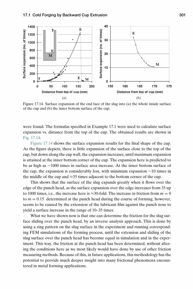
17.1 Cold Forging by Backward Cup Extrusion 301
(a) (b)
Figure 17.14. Surface expansion of the end face of the slug into (a) the whole inside surfaceof the cup and (b) the inner bottom surface of the cup.
were found. The formulas specified in Example 17.1 were used to calculate surfaceexpansion vs. distance from the top of the cup. The obtained results are shown inFig. 17.14.
Figure 17.14 shows the surface expansion results for the final shape of the cup.As the figure depicts, there is little expansion of the surface close to the top of thecup, but down along the cup wall, the expansion increases, until maximum expansionis attained at the inner bottom corner of the cup. The expansion here is predicted tobe as high as ∼1000 times in surface area increase. At the inner bottom surface ofthe cup, the expansion is considerably less, with minimum expansion ∼10 times inthe middle of the cup and ≈35 times adjacent to the bottom corner of the cup.
This shows that the surface of the slug expands greatly when it flows over theedge of the punch head, as the surface expansion over the edge increases from 35 upto 1000 times, i.e., the increase here is ≈30-fold. The increase in friction from m = 0to m = 0.15 determined at the punch head during the course of forming, however,seems to be caused by the extension of the lubricant film against the punch nose toyield a surface increase in the range of 10–35 times.
What we have shown now is that one can determine the friction for the slug sur-face sliding over the punch head, by an inverse analysis approach. This is done byusing a ring pattern on the slug surface in the experiment and running correspond-ing FEM simulations of the forming process, until the extension and sliding of theslug surface over the punch head has become equal in simulation and in the exper-iment. This way, the friction at the punch head has been determined, without alter-ing the conditions here as we most likely would have done by use of other frictionmeasuring methods. Because of this, in future applications, this methodology has thepotential to provide much deeper insight into many frictional phenomena encoun-tered in metal forming applications.
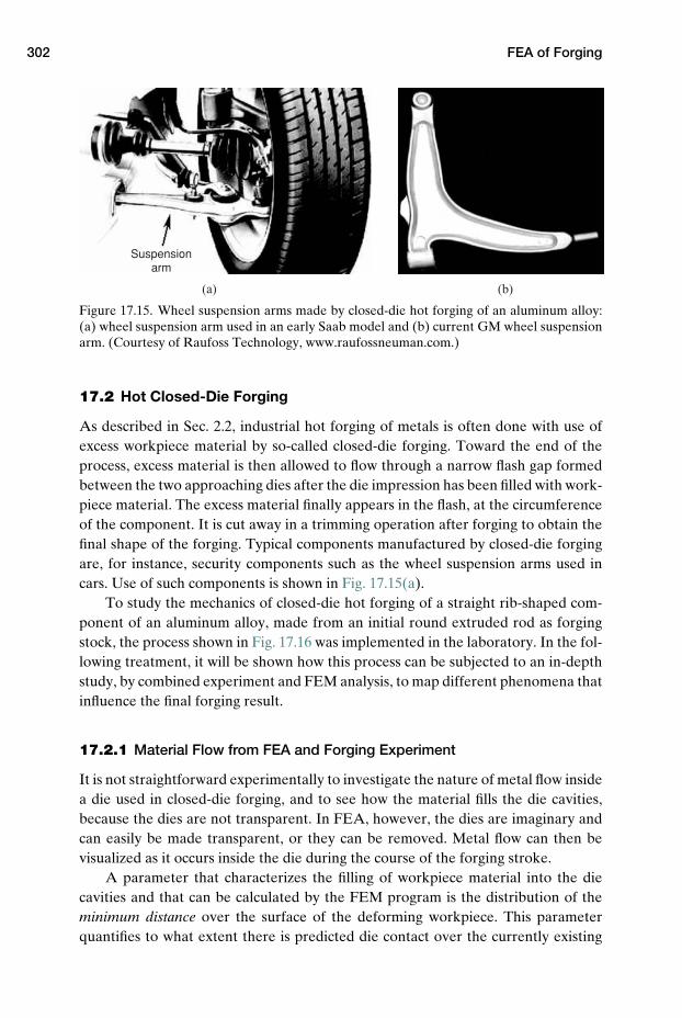
302 FEA of Forging
(a) (b)
Suspension arm
Figure 17.15. Wheel suspension arms made by closed-die hot forging of an aluminum alloy:(a) wheel suspension arm used in an early Saab model and (b) current GM wheel suspensionarm. (Courtesy of Raufoss Technology, www.raufossneuman.com.)
17.2 Hot Closed-Die Forging
As described in Sec. 2.2, industrial hot forging of metals is often done with use ofexcess workpiece material by so-called closed-die forging. Toward the end of theprocess, excess material is then allowed to flow through a narrow flash gap formedbetween the two approaching dies after the die impression has been filled with work-piece material. The excess material finally appears in the flash, at the circumferenceof the component. It is cut away in a trimming operation after forging to obtain thefinal shape of the forging. Typical components manufactured by closed-die forgingare, for instance, security components such as the wheel suspension arms used incars. Use of such components is shown in Fig. 17.15(a).
To study the mechanics of closed-die hot forging of a straight rib-shaped com-ponent of an aluminum alloy, made from an initial round extruded rod as forgingstock, the process shown in Fig. 17.16 was implemented in the laboratory. In the fol-lowing treatment, it will be shown how this process can be subjected to an in-depthstudy, by combined experiment and FEM analysis, to map different phenomena thatinfluence the final forging result.
17.2.1 Material Flow from FEA and Forging Experiment
It is not straightforward experimentally to investigate the nature of metal flow insidea die used in closed-die forging, and to see how the material fills the die cavities,because the dies are not transparent. In FEA, however, the dies are imaginary andcan easily be made transparent, or they can be removed. Metal flow can then bevisualized as it occurs inside the die during the course of the forging stroke.
A parameter that characterizes the filling of workpiece material into the diecavities and that can be calculated by the FEM program is the distribution of theminimum distance over the surface of the deforming workpiece. This parameterquantifies to what extent there is predicted die contact over the currently existing
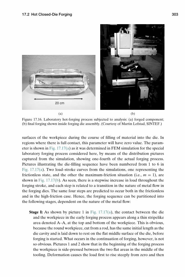
17.2 Hot Closed-Die Forging 303
20 cm
(a) (b)
20 cm
Figure 17.16. Laboratory hot-forging process subjected to analysis: (a) forged component;(b) final forging shown inside forging die assembly. (Courtesy of Martin Lefstad, SINTEF.)
surfaces of the workpiece during the course of filling of material into the die. Inregions where there is full contact, this parameter will have zero value. The param-eter is shown in Fig. 17.17(a) as it was determined in FEM simulation for the speciallaboratory forging process considered here, by means of the distribution picturescaptured from the simulation, showing one-fourth of the actual forging process.Pictures illustrating the die-filling sequence have been numbered from 1 to 6 inFig. 17.17(a). Two load–stroke curves from the simulations, one representing thefrictionless state, and the other the maximum-friction situation (i.e., m = 1), areshown in Fig. 17.17(b). As seen, there is a stepwise increase in load throughout theforging stroke, and each step is related to a transition in the nature of metal flow inthe forging dies. The same four steps are predicted to occur both in the frictionlessand in the high-friction case. Hence, the forging sequence can be partitioned intothe following stages, dependent on the nature of the metal flow:
Stage I: As shown by picture 1 in Fig. 17.17(a), the contact between the dieand the workpiece in the early forging process appears along a thin stripelikearea denoted A–A, at the top and bottom of the workpiece. This is obvious,because the round workpiece, cut from a rod, has the same initial length as thedie cavity and is laid down to rest on the flat middle surface of the die, beforeforging is started. What occurs in the continuation of forging, however, is notso obvious. Pictures 1 and 2 show that in the beginning of the forging processthe workpiece is side-pressed between the two flat areas in the middle of thetooling. Deformation causes the load first to rise steeply from zero and then
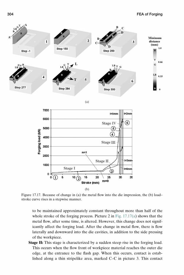
304 FEA of Forging
(a)
(b)
-
Figure 17.17. Because of change in (a) the metal flow into the die impression, the (b) load–stroke curve rises in a stepwise manner.
to be maintained approximately constant throughout more than half of thewhole stroke of the forging process. Picture 2 in Fig. 17.17(a) shows that themetal flow, after some time, is altered. However, this change does not signif-icantly affect the forging load. After the change in metal flow, there is flowlaterally and downward into the die cavities, in addition to the side pressingof the workpiece.
Stage II: This stage is characterized by a sudden steep rise in the forging load.This occurs when the flow front of workpiece material reaches the outer dieedge, at the entrance to the flash gap. When this occurs, contact is estab-lished along a thin stripelike area, marked C–C in picture 3. This contact
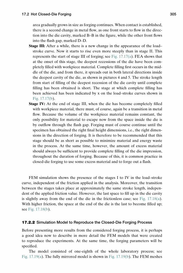
17.2 Hot Closed-Die Forging 305
area gradually grows in size as forging continues. When contact is established,there is a second change in metal flow, as one front starts to flow in the direc-tion into the die cavity, marked B–B in the figure, while the other front flowsinto the flash gap, marked D–D.
Stage III: After a while, there is a new change in the appearance of the load–stroke curve. Now it starts to rise even more steeply than in stage II. Thisrepresents the start of stage III of forging; see Fig. 17.17(a). FEA shows thatat the onset of this stage, the deepest recessions of the die have been com-pletely filled with workpiece material. Complete filling first occurs in the mid-dle of the die, and from there, it spreads out in both lateral directions insidethe deepest cavity of the die, as shown in pictures 4 and 5. The stroke lengthfrom start of filling of the deepest recession of the die cavity until completefilling has been obtained is short. The stage at which complete filling hasbeen achieved has been indicated by x on the load–stroke curves shown inFig. 17.17(b).
Stage IV: At the end of stage III, when the die has become completely filledwith workpiece material, there must, of course, again be a transition in metalflow. Because the volume of the workpiece material remains constant, theonly possibility for material to escape now from the space inside the die isby outflow through the flash gap. Forging must of course continue until thespecimen has obtained the right final height dimensions, i.e., the right dimen-sions in the direction of forging. It is therefore to be recommended that thisstage should be as short as possible to minimize material and energy wastein the process. At the same time, however, the amount of excess materialshould always be sufficient to provide complete filling of the die impression,throughout the duration of forging. Because of this, it is common practice inclosed-die forging to use some excess material and to forge out a flash.
FEM simulation shows the presence of the stages I to IV in the load–strokecurve, independent of the friction applied in the analysis. Moreover, the transitionbetween the stages takes place at approximately the same stroke length, indepen-dent of the applied friction value. However, the last space to fill up in the die cavityis slightly away from the end of the die in the frictionless case; see Fig. 17.18(a).With higher friction, the space at the end of the die is the last to become filled up;see Fig. 17.18(b).
17.2.2 Simulation Model to Reproduce the Closed-Die Forging Process
Before presenting more results from the considered forging process, it is perhapsa good idea now to describe in more detail the FEM models that were createdto reproduce the experiments. At the same time, the forging parameters will bespecified.
The model consisted of one-eighth of the whole laboratory process; seeFig. 17.19(a). The fully mirrored model is shown in Fig. 17.19(b). The FEM meshes
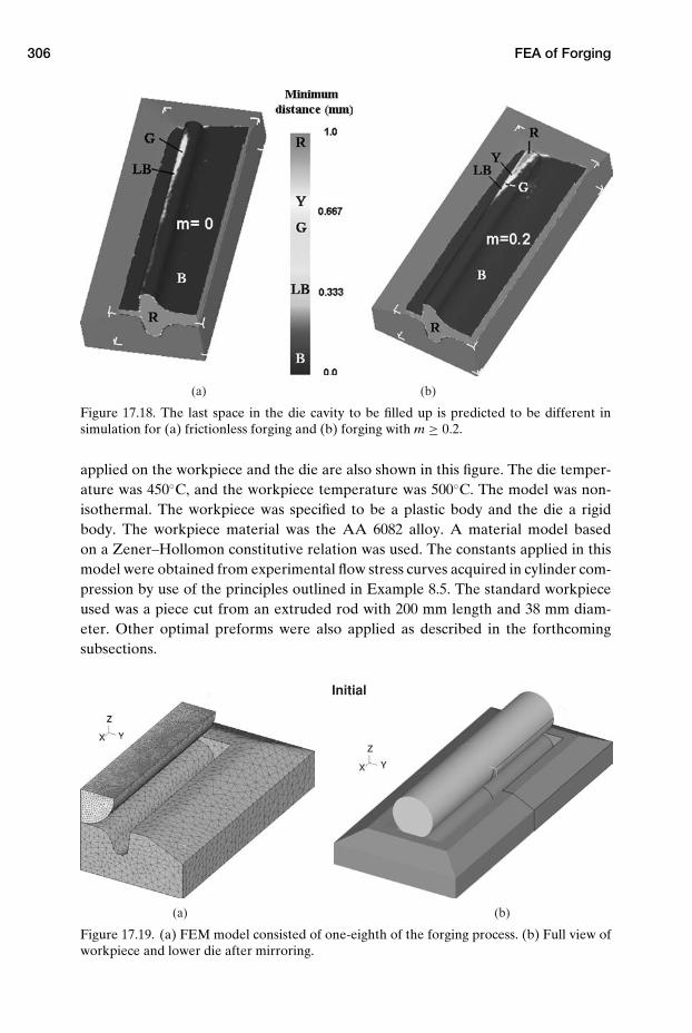
306 FEA of Forging
(a) (b)
Figure 17.18. The last space in the die cavity to be filled up is predicted to be different insimulation for (a) frictionless forging and (b) forging with m ≥ 0.2.
applied on the workpiece and the die are also shown in this figure. The die temper-ature was 450◦C, and the workpiece temperature was 500◦C. The model was non-isothermal. The workpiece was specified to be a plastic body and the die a rigidbody. The workpiece material was the AA 6082 alloy. A material model basedon a Zener–Hollomon constitutive relation was used. The constants applied in thismodel were obtained from experimental flow stress curves acquired in cylinder com-pression by use of the principles outlined in Example 8.5. The standard workpieceused was a piece cut from an extruded rod with 200 mm length and 38 mm diam-eter. Other optimal preforms were also applied as described in the forthcomingsubsections.
(a) (b)
Initial
Figure 17.19. (a) FEM model consisted of one-eighth of the forging process. (b) Full view ofworkpiece and lower die after mirroring.
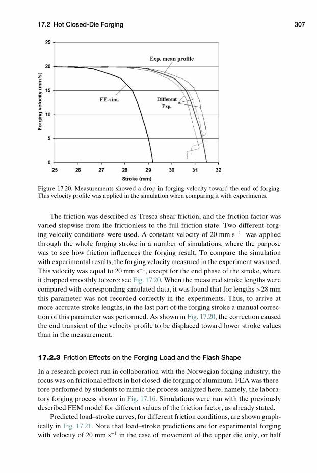
17.2 Hot Closed-Die Forging 307
Figure 17.20. Measurements showed a drop in forging velocity toward the end of forging.This velocity profile was applied in the simulation when comparing it with experiments.
The friction was described as Tresca shear friction, and the friction factor wasvaried stepwise from the frictionless to the full friction state. Two different forg-ing velocity conditions were used. A constant velocity of 20 mm s−1 was appliedthrough the whole forging stroke in a number of simulations, where the purposewas to see how friction influences the forging result. To compare the simulationwith experimental results, the forging velocity measured in the experiment was used.This velocity was equal to 20 mm s−1, except for the end phase of the stroke, whereit dropped smoothly to zero; see Fig. 17.20. When the measured stroke lengths werecompared with corresponding simulated data, it was found that for lengths >28 mmthis parameter was not recorded correctly in the experiments. Thus, to arrive atmore accurate stroke lengths, in the last part of the forging stroke a manual correc-tion of this parameter was performed. As shown in Fig. 17.20, the correction causedthe end transient of the velocity profile to be displaced toward lower stroke valuesthan in the measurement.
17.2.3 Friction Effects on the Forging Load and the Flash Shape
In a research project run in collaboration with the Norwegian forging industry, thefocus was on frictional effects in hot closed-die forging of aluminum. FEA was there-fore performed by students to mimic the process analyzed here, namely, the labora-tory forging process shown in Fig. 17.16. Simulations were run with the previouslydescribed FEM model for different values of the friction factor, as already stated.
Predicted load–stroke curves, for different friction conditions, are shown graph-ically in Fig. 17.21. Note that load–stroke predictions are for experimental forgingwith velocity of 20 mm s−1 in the case of movement of the upper die only, or half
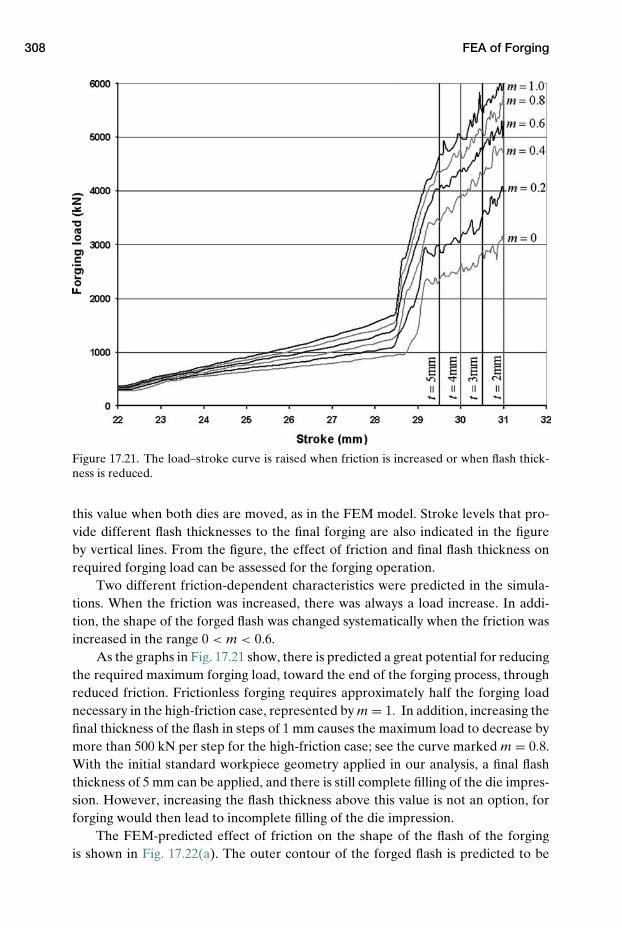
308 FEA of Forging
Figure 17.21. The load–stroke curve is raised when friction is increased or when flash thick-ness is reduced.
this value when both dies are moved, as in the FEM model. Stroke levels that pro-vide different flash thicknesses to the final forging are also indicated in the figureby vertical lines. From the figure, the effect of friction and final flash thickness onrequired forging load can be assessed for the forging operation.
Two different friction-dependent characteristics were predicted in the simula-tions. When the friction was increased, there was always a load increase. In addi-tion, the shape of the forged flash was changed systematically when the friction wasincreased in the range 0 < m < 0.6.
As the graphs in Fig. 17.21 show, there is predicted a great potential for reducingthe required maximum forging load, toward the end of the forging process, throughreduced friction. Frictionless forging requires approximately half the forging loadnecessary in the high-friction case, represented by m = 1. In addition, increasing thefinal thickness of the flash in steps of 1 mm causes the maximum load to decrease bymore than 500 kN per step for the high-friction case; see the curve marked m = 0.8.With the initial standard workpiece geometry applied in our analysis, a final flashthickness of 5 mm can be applied, and there is still complete filling of the die impres-sion. However, increasing the flash thickness above this value is not an option, forforging would then lead to incomplete filling of the die impression.
The FEM-predicted effect of friction on the shape of the flash of the forgingis shown in Fig. 17.22(a). The outer contour of the forged flash is predicted to be
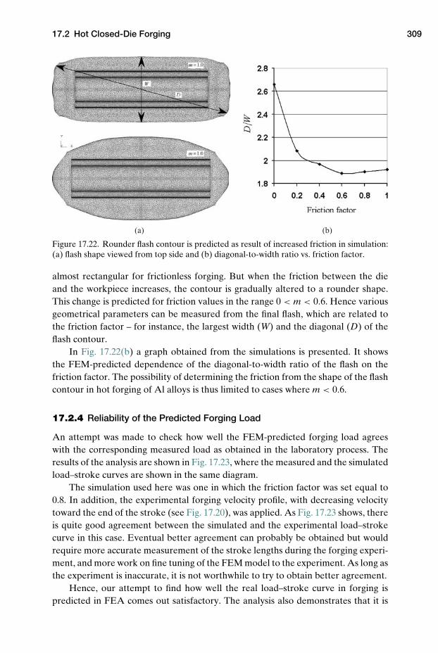
17.2 Hot Closed-Die Forging 309
(a) (b)
Figure 17.22. Rounder flash contour is predicted as result of increased friction in simulation:(a) flash shape viewed from top side and (b) diagonal-to-width ratio vs. friction factor.
almost rectangular for frictionless forging. But when the friction between the dieand the workpiece increases, the contour is gradually altered to a rounder shape.This change is predicted for friction values in the range 0 < m < 0.6. Hence variousgeometrical parameters can be measured from the final flash, which are related tothe friction factor – for instance, the largest width (W) and the diagonal (D) of theflash contour.
In Fig. 17.22(b) a graph obtained from the simulations is presented. It showsthe FEM-predicted dependence of the diagonal-to-width ratio of the flash on thefriction factor. The possibility of determining the friction from the shape of the flashcontour in hot forging of Al alloys is thus limited to cases where m < 0.6.
17.2.4 Reliability of the Predicted Forging Load
An attempt was made to check how well the FEM-predicted forging load agreeswith the corresponding measured load as obtained in the laboratory process. Theresults of the analysis are shown in Fig. 17.23, where the measured and the simulatedload–stroke curves are shown in the same diagram.
The simulation used here was one in which the friction factor was set equal to0.8. In addition, the experimental forging velocity profile, with decreasing velocitytoward the end of the stroke (see Fig. 17.20), was applied. As Fig. 17.23 shows, thereis quite good agreement between the simulated and the experimental load–strokecurve in this case. Eventual better agreement can probably be obtained but wouldrequire more accurate measurement of the stroke lengths during the forging experi-ment, and more work on fine tuning of the FEM model to the experiment. As long asthe experiment is inaccurate, it is not worthwhile to try to obtain better agreement.
Hence, our attempt to find how well the real load–stroke curve in forging ispredicted in FEA comes out satisfactory. The analysis also demonstrates that it is
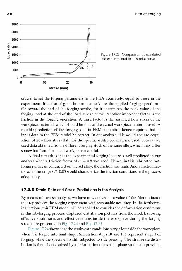
310 FEA of Forging
Figure 17.23. Comparison of simulatedand experimental load–stroke curves.
crucial to set the forging parameters in the FEA accurately, equal to those in theexperiment. It is also of great importance to know the applied forging speed pro-file toward the end of the forging stroke, for it determines the peak value of theforging load at the end of the load–stroke curve. Another important factor is thefriction in the forging operation. A third factor is the assumed flow stress of theworkpiece material, which should be that of the actual workpiece material used. Areliable prediction of the forging load in FEM-simulation hence requires that allinput data to the FEM model be correct. In our analysis, this would require acqui-sition of new flow stress data for the specific workpiece material used, because weused data obtained from a different forging stock of the same alloy, which may differsomewhat from the actual workpiece material.
A final remark is that the experimental forging load was well predicted in ouranalysis when a friction factor of m = 0.8 was used. Hence, in this lubricated hot-forging process, conducted on the Al alloy, the friction was high. And a friction fac-tor m in the range 0.7–0.85 would characterize the friction conditions in the processadequately.
17.2.5 Strain-Rate and Strain Predictions in the Analysis
By means of inverse analysis, we have now arrived at a value of the friction factorthat reproduces the forging experiment with reasonable accuracy. In the forthcom-ing sections, this FEM model will be applied to consider the deformation conditionsin this rib-forging process. Captured distribution pictures from the model, showingeffective strain rates and effective strains inside the workpiece during the forgingstroke, are presented in Fig. 17.24 and Fig. 17.25.
Figure 17.24 shows that the strain-rate conditions vary a lot inside the workpiecewhen it is forged into final shape. Simulation steps 10 and 135 represent stage I offorging, while the specimen is still subjected to side pressing. The strain-rate distri-bution is then characterized by a deformation cross as in plane strain compression;
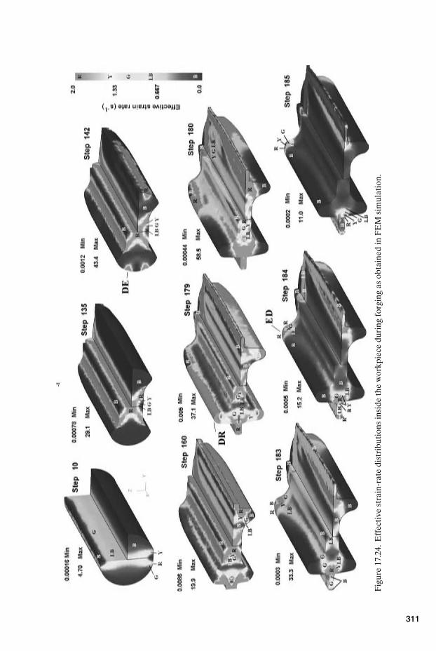
Fig
ure
17.2
4.E
ffec
tive
stra
in-r
ate
dist
ribu
tion
sin
side
the
wor
kpie
cedu
ring
forg
ing
asob
tain
edin
FE
Msi
mul
atio
n.
311
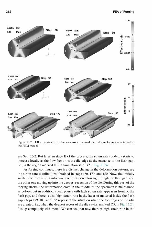
312 FEA of Forging
Figure 17.25. Effective strain distributions inside the workpiece during forging as obtained inthe FEM model.
see Sec. 3.5.2. But later, in stage II of the process, the strain rate suddenly starts toincrease locally as the flow front hits the die edge at the entrance to the flash gap,i.e., in the region marked DE in simulation step 142 in Fig. 17.24.
As forging continues, there is a distinct change in the deformation pattern: seethe strain-rate distributions obtained in steps 160, 179, and 180. Now, the initiallysingle flow front is split into two new fronts, one flowing through the flash gap, andthe other one moving up into the deepest recession of the die. During this part of theforging stroke, the deformation cross in the middle of the specimen is maintainedas before, but in addition, shear planes with high strain rate appear in front of theflash gap, and there is also high strain rate in the layer of material inside the flashgap. Steps 179, 180, and 183 represent the situation when the top ridges of the ribsare created, i.e., when the deepest recess of the die cavity, marked DR in Fig. 17.24,fills up completely with metal. We can see that now there is high strain rate in the
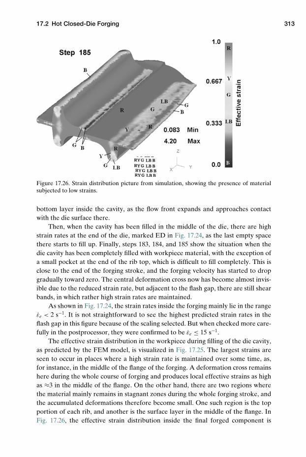
17.2 Hot Closed-Die Forging 313
Figure 17.26. Strain distribution picture from simulation, showing the presence of materialsubjected to low strains.
bottom layer inside the cavity, as the flow front expands and approaches contactwith the die surface there.
Then, when the cavity has been filled in the middle of the die, there are highstrain rates at the end of the die, marked ED in Fig. 17.24, as the last empty spacethere starts to fill up. Finally, steps 183, 184, and 185 show the situation when thedie cavity has been completely filled with workpiece material, with the exception ofa small pocket at the end of the rib top, which is difficult to fill completely. This isclose to the end of the forging stroke, and the forging velocity has started to dropgradually toward zero. The central deformation cross now has become almost invis-ible due to the reduced strain rate, but adjacent to the flash gap, there are still shearbands, in which rather high strain rates are maintained.
As shown in Fig. 17.24, the strain rates inside the forging mainly lie in the rangeεe < 2 s−1. It is not straightforward to see the highest predicted strain rates in theflash gap in this figure because of the scaling selected. But when checked more care-fully in the postprocessor, they were confirmed to be εe ≤ 15 s−1.
The effective strain distribution in the workpiece during filling of the die cavity,as predicted by the FEM model, is visualized in Fig. 17.25. The largest strains areseen to occur in places where a high strain rate is maintained over some time, as,for instance, in the middle of the flange of the forging. A deformation cross remainshere during the whole course of forging and produces local effective strains as highas ≈3 in the middle of the flange. On the other hand, there are two regions wherethe material mainly remains in stagnant zones during the whole forging stroke, andthe accumulated deformations therefore become small. One such region is the topportion of each rib, and another is the surface layer in the middle of the flange. InFig. 17.26, the effective strain distribution inside the final forged component is
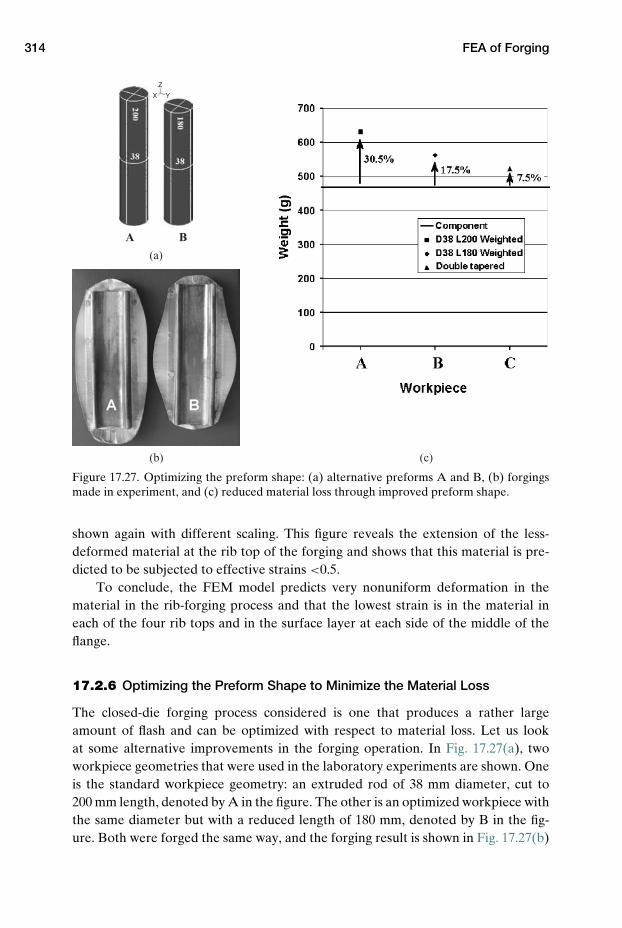
314 FEA of Forging
A B
(a)
(b) (c)
X Y
Z
Figure 17.27. Optimizing the preform shape: (a) alternative preforms A and B, (b) forgingsmade in experiment, and (c) reduced material loss through improved preform shape.
shown again with different scaling. This figure reveals the extension of the less-deformed material at the rib top of the forging and shows that this material is pre-dicted to be subjected to effective strains <0.5.
To conclude, the FEM model predicts very nonuniform deformation in thematerial in the rib-forging process and that the lowest strain is in the material ineach of the four rib tops and in the surface layer at each side of the middle of theflange.
17.2.6 Optimizing the Preform Shape to Minimize the Material Loss
The closed-die forging process considered is one that produces a rather largeamount of flash and can be optimized with respect to material loss. Let us lookat some alternative improvements in the forging operation. In Fig. 17.27(a), twoworkpiece geometries that were used in the laboratory experiments are shown. Oneis the standard workpiece geometry: an extruded rod of 38 mm diameter, cut to200 mm length, denoted by A in the figure. The other is an optimized workpiece withthe same diameter but with a reduced length of 180 mm, denoted by B in the fig-ure. Both were forged the same way, and the forging result is shown in Fig. 17.27(b)
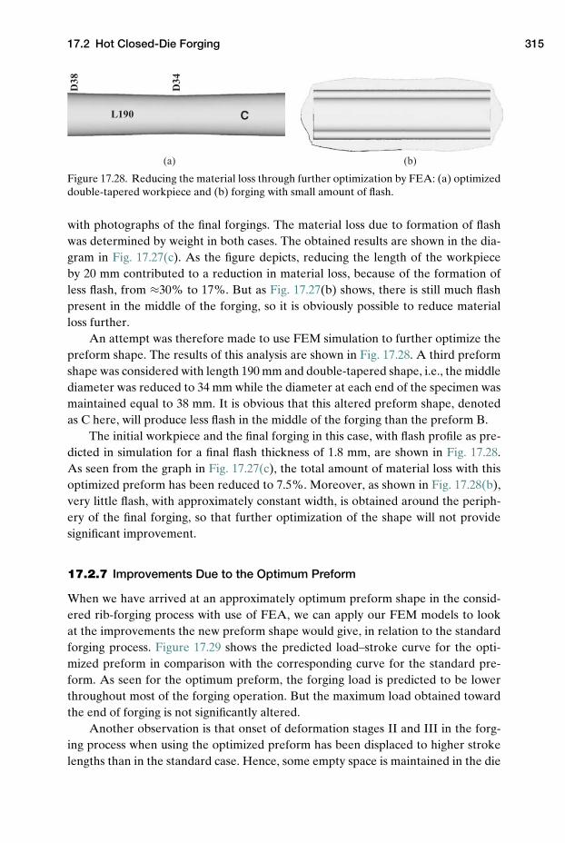
17.2 Hot Closed-Die Forging 315
D38
D34
L190 C
(a) (b)
Figure 17.28. Reducing the material loss through further optimization by FEA: (a) optimizeddouble-tapered workpiece and (b) forging with small amount of flash.
with photographs of the final forgings. The material loss due to formation of flashwas determined by weight in both cases. The obtained results are shown in the dia-gram in Fig. 17.27(c). As the figure depicts, reducing the length of the workpieceby 20 mm contributed to a reduction in material loss, because of the formation ofless flash, from ≈30% to 17%. But as Fig. 17.27(b) shows, there is still much flashpresent in the middle of the forging, so it is obviously possible to reduce materialloss further.
An attempt was therefore made to use FEM simulation to further optimize thepreform shape. The results of this analysis are shown in Fig. 17.28. A third preformshape was considered with length 190 mm and double-tapered shape, i.e., the middlediameter was reduced to 34 mm while the diameter at each end of the specimen wasmaintained equal to 38 mm. It is obvious that this altered preform shape, denotedas C here, will produce less flash in the middle of the forging than the preform B.
The initial workpiece and the final forging in this case, with flash profile as pre-dicted in simulation for a final flash thickness of 1.8 mm, are shown in Fig. 17.28.As seen from the graph in Fig. 17.27(c), the total amount of material loss with thisoptimized preform has been reduced to 7.5%. Moreover, as shown in Fig. 17.28(b),very little flash, with approximately constant width, is obtained around the periph-ery of the final forging, so that further optimization of the shape will not providesignificant improvement.
17.2.7 Improvements Due to the Optimum Preform
When we have arrived at an approximately optimum preform shape in the consid-ered rib-forging process with use of FEA, we can apply our FEM models to lookat the improvements the new preform shape would give, in relation to the standardforging process. Figure 17.29 shows the predicted load–stroke curve for the opti-mized preform in comparison with the corresponding curve for the standard pre-form. As seen for the optimum preform, the forging load is predicted to be lowerthroughout most of the forging operation. But the maximum load obtained towardthe end of forging is not significantly altered.
Another observation is that onset of deformation stages II and III in the forg-ing process when using the optimized preform has been displaced to higher strokelengths than in the standard case. Hence, some empty space is maintained in the die
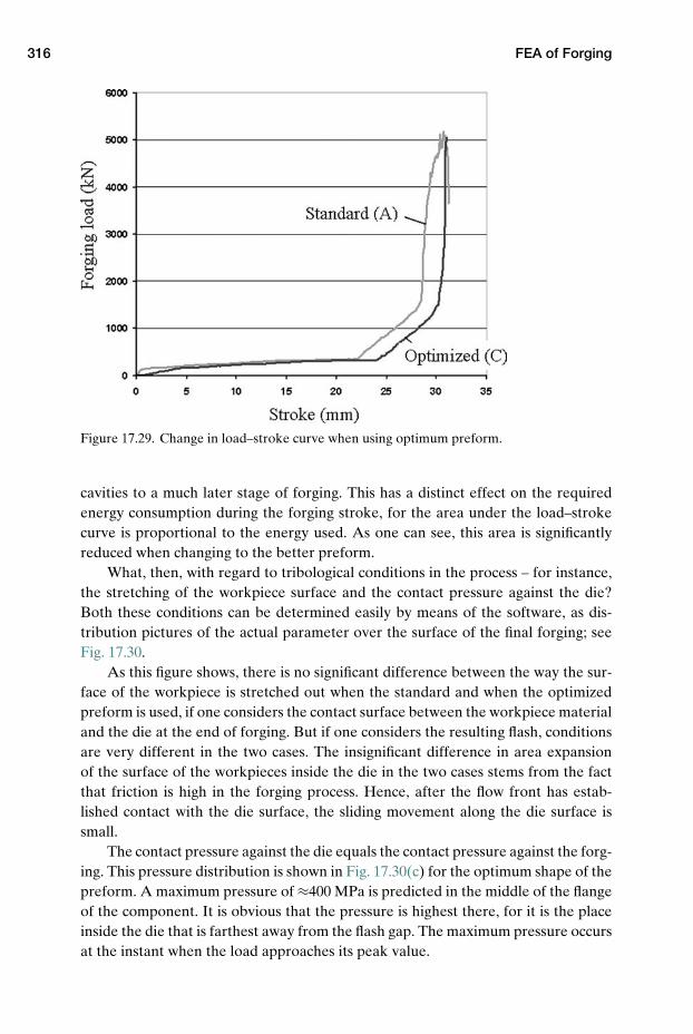
316 FEA of Forging
Figure 17.29. Change in load–stroke curve when using optimum preform.
cavities to a much later stage of forging. This has a distinct effect on the requiredenergy consumption during the forging stroke, for the area under the load–strokecurve is proportional to the energy used. As one can see, this area is significantlyreduced when changing to the better preform.
What, then, with regard to tribological conditions in the process – for instance,the stretching of the workpiece surface and the contact pressure against the die?Both these conditions can be determined easily by means of the software, as dis-tribution pictures of the actual parameter over the surface of the final forging; seeFig. 17.30.
As this figure shows, there is no significant difference between the way the sur-face of the workpiece is stretched out when the standard and when the optimizedpreform is used, if one considers the contact surface between the workpiece materialand the die at the end of forging. But if one considers the resulting flash, conditionsare very different in the two cases. The insignificant difference in area expansionof the surface of the workpieces inside the die in the two cases stems from the factthat friction is high in the forging process. Hence, after the flow front has estab-lished contact with the die surface, the sliding movement along the die surface issmall.
The contact pressure against the die equals the contact pressure against the forg-ing. This pressure distribution is shown in Fig. 17.30(c) for the optimum shape of thepreform. A maximum pressure of ≈400 MPa is predicted in the middle of the flangeof the component. It is obvious that the pressure is highest there, for it is the placeinside the die that is farthest away from the flash gap. The maximum pressure occursat the instant when the load approaches its peak value.
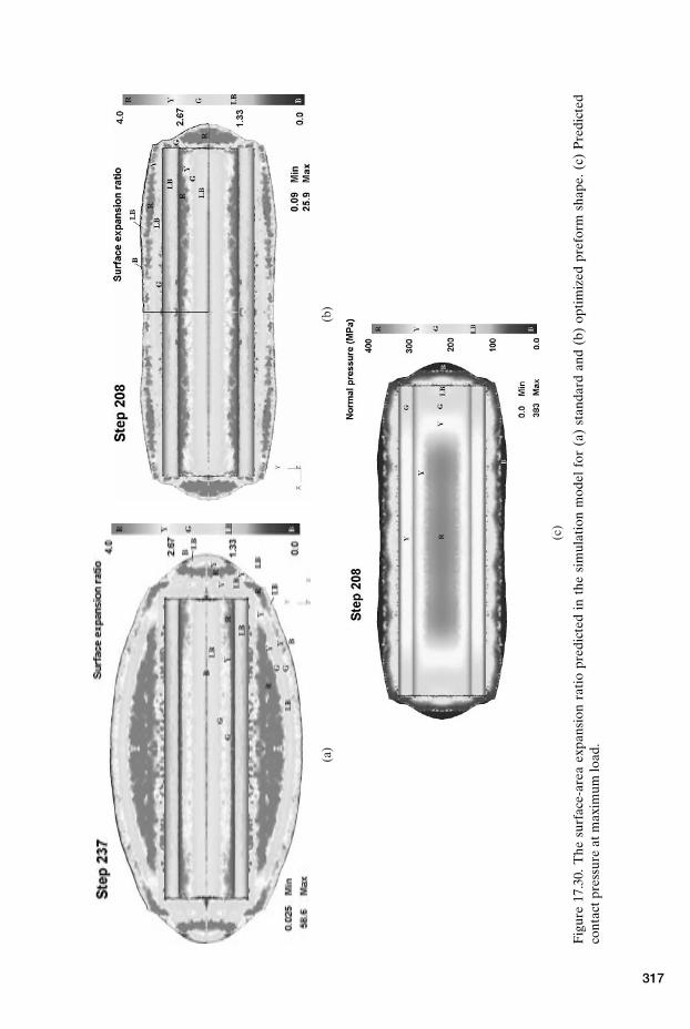
(a)
(b)
(c)
Fig
ure
17.3
0.T
hesu
rfac
e-ar
eaex
pans
ion
rati
opr
edic
ted
inth
esi
mul
atio
nm
odel
for
(a)
stan
dard
and
(b)
opti
miz
edpr
efor
msh
ape.
(c)
Pre
dict
edco
ntac
tpre
ssur
eat
max
imum
load
.
317
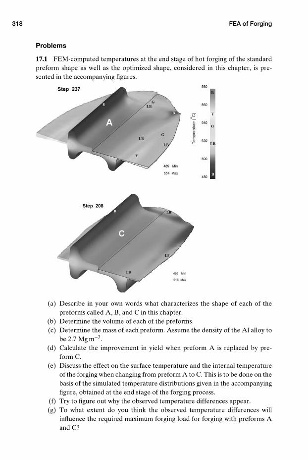
318 FEA of Forging
Problems
17.1 FEM-computed temperatures at the end stage of hot forging of the standardpreform shape as well as the optimized shape, considered in this chapter, is pre-sented in the accompanying figures.
(a) Describe in your own words what characterizes the shape of each of thepreforms called A, B, and C in this chapter.
(b) Determine the volume of each of the preforms.(c) Determine the mass of each preform. Assume the density of the Al alloy to
be 2.7 Mg m−3.(d) Calculate the improvement in yield when preform A is replaced by pre-
form C.(e) Discuss the effect on the surface temperature and the internal temperature
of the forging when changing from preform A to C. This is to be done on thebasis of the simulated temperature distributions given in the accompanyingfigure, obtained at the end stage of the forging process.
(f) Try to figure out why the observed temperature differences appear.(g) To what extent do you think the observed temperature differences will
influence the required maximum forging load for forging with preforms Aand C?

References 319
NOTES
1. Production Engineering Association (U.K.), PERA report No. 102.2. Benani, B., and Bay, N.: “Limits of lubrication in backward can extrusion: Analysis
by finite-element method and physical modeling experiments,” J. Materials ProcessingTechnology, Vol. 61, 1996, pp. 275–286.
3. Uyyuru, R., and Valberg, H.: “Physical and numerical analysis of metal flow over thepunch head in backward cup extrusion of aluminium,” J. Materials Processing Technol-ogy, Vol. 172, 2006, pp. 312–318.
REFERENCES
Nolte, D.: “Analysis of Aluminium Hot Forging,” Ph.D. thesis, Norwegian University of Sci-ence and Technology (NTNU), 2004.
Uyyuru, R. K.: “Engineering the Friction and Forming Mechanics in Cold Aluminium Form-ing – Use of Modelling Techniques,” Ph.D. thesis, Norwegian University of Science andTechnology (NTNU), 2003.
Wey, E.: “New developments in FE simulation of industrial forging processes,” 19th Int.Forging Congr., Chicago, 2008.
18 Extrusion
As previously described in Ch. 2, extrusion is done by placing a piece of metal ofgood formability, called a billet, in a hardened steel container. In direct extrusion, aram is then pushed from the back end of the container, so the billet is forced againsta die placed at the other end of the container. The die has a hole in its middle, andas the billet is pushed forward, the front part of it starts to flow into the hole, andthen out into the space at the exit side of the hole. Here it appears as a continuousextrusion with cross section approximately that of the hole. The longitudinal shapeobtained in this process is generally called an extruded profile, or an extrudate. Thismetal forming technique is hence used to manufacture products with constant cross-sectional shape along their length, either as massive or hollow profiles, or as rod,tube, wire, or strip.
Because the flow stress is reduced when metals are heated, and workability alsomost commonly increases, extrusion is usually conducted as hot forming. Extru-sion can either be done as forward (direct) or backward (indirect) extrusion; seeCh. 2.2.5. In forward extrusion, the material is pushed through the container and thedie by means of the ram, whereas in backward extrusion, the die is placed in frontof the hollow ram, whereafter the die is pushed into the billet. The billet materialremains stationary inside the container then until it is approached by the movingdie; the billet then starts to flow through the die, i.e., in the reverse direction ofthe ram movement and must therefore be taken out through the ram, which mustbe hollow.
In this chapter, some practical aspects of industrial extrusion will first bedescribed. It is important to be able to predict the required extrusion force, becausethat force is very large and sets a limit to how fast the extrusion process can beconducted without exceeding the maximum available force in the press. In the lastpart of this chapter, theory will therefore be used to develop an expression for therequired extrusion force. The expression is useful in that it shows how the requiredforce is influenced by different extrusion parameters.
320
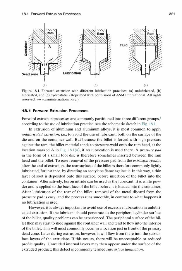
18.1 Forward Extrusion Processes 321
(a) (b) (c)
Figure 18.1. Forward extrusion with different lubrication practices: (a) unlubricated, (b)lubricated, and (c) hydrostatic. (Reprinted with permission of ASM International. All rightsreserved. www.asminternational.org.)
18.1 Forward Extrusion Processes
Forward extrusion processes are commonly partitioned into three different groups,1
according to the use of lubrication practice; see the schematic sketch in Fig. 18.1.In extrusion of aluminum and aluminum alloys, it is most common to apply
unlubricated extrusion, i.e., to avoid the use of lubricant, both on the surface of thedie and on the container wall. But because the billet is forced with high pressureagainst the ram, the billet material tends to pressure-weld onto the ram head, at thelocation marked A in Fig. 18.1(a), if no lubrication is used there. A pressure padin the form of a small tool disc is therefore sometimes inserted between the ramhead and the billet. To ease removal of the pressure pad from the extrusion residueafter the end of extrusion, the rear surface of the billet is therefore commonly lightlylubricated, for instance, by directing an acetylene flame against it. In this way, a thinlayer of soot is deposited onto this surface, before insertion of the billet into thecontainer. Alternatively, boron nitride can be used as the lubricant. It is white pow-der and is applied to the back face of the billet before it is loaded into the container.After lubrication of the rear of the billet, removal of the metal discard from thepressure pad is easy, and the process runs smoothly, in contrast to what happens ifno lubrication is used.
However, it is always important to avoid use of excessive lubrication in unlubri-cated extrusion. If the lubricant should penetrate to the peripheral cylinder surfaceof the billet, quality problems can be experienced. The peripheral surface of the bil-let then may start to slide against the container wall and tend to flow into the interiorof the billet. This will most commonly occur in a location just in front of the primarydead zone. Later during extrusion, however, it will flow from there into the subsur-face layers of the extrudate. If this occurs, there will be unacceptable or reducedprofile quality. Unwelded internal layers may then appear under the surface of theextruded product; this defect is commonly termed subsurface lamination.

322 Extrusion
In unlubricated hot extrusion, flat-faced dies are most commonly used; seeFig. 18.1(a). Without lubrication, as mentioned in Ch. 12, there will be high frictionbetween the workpiece and the die and container. With such conditions, a primarydead zone will form inside the billet volume during extrusion, in the corner betweenthe die and the container. In unlubricated extrusion, the peripheral surface layerof the billet then will tend to accumulate inside the container during the course ofextrusion and will not flow out into the extrudate. This is advantageous in that theperipheral layer usually has lower metallurgical quality than the rest of the billet. Itoften contains intermetallic inclusions, which – if they appear on the surface of theprofile – can yield extrusions with bad surface quality.
A less common extrusion process is lubricated extrusion [see Fig. 18.1(b)], inwhich conical, wedge-shaped dies are used. Dead zones will not form in lubricatedextrusion; instead, the outer surface layer of the billet will slide over the die surfaceand will flow out into the extrusion, where it will form the outer surface layer ofthe extrusion. The characteristic shear zone formed inside the billet in unlubricatedextrusion will not be present the same way in lubricated extrusion.
Material flow in unlubricated extrusion is characterized by the formation ofa primary and a secondary deformation zone, which make up the volume of theextruding billet; see Fig. 12.7. In lubricated extrusion, however, the secondary defor-mation zone will be absent, or at least not well developed. Because of this differencein metal flow, the resulting extrusion in lubricated extrusion has much more homo-geneous deformations than in unlubricated extrusion.
In both processes, the billet metal, which initially filled the volume ahead ofthe die hole, will be subjected to less deformation than metal farther behind. Thismaterial will only move through part of the primary deformation zone during extru-sion. Because of this, the very front end of the rod will only be subjected to smalldeformation, because this metal is near the die hole when extrusion begins. Afterthe initial volume of the primary deformation zone has flowed out, the deformationof the rest of the rod will be much more uniform over the length of the extrusionthan before. It is common to cut away and discard a short length of the front end ofthe extrusion.
In hydrostatic extrusion, the pressure is transferred from the die onto the bil-let through a fluid, which fills the space between the billet and the ram head; seeFig. 18.1(c). During this extrusion process, the fluid will also act as a lubricant andwill be squeezed under high pressure into the interface between the billet and thedie. Because of this, there will be efficient lubrication in this extrusion process.
Lubricated and (especially) hydrostatic extrusion are much more complex pro-cesses to run than unlubricated extrusion and are mainly used for low-ductility mate-rials, which tend to crack in conventional unlubricated extrusion.
18.2 Hot Unlubricated Extrusion of Aluminum Alloys
As mentioned, Al and Al alloys are usually extruded by means of unlubricated hotextrusion. Both forward and backward extrusion are used for this purpose.
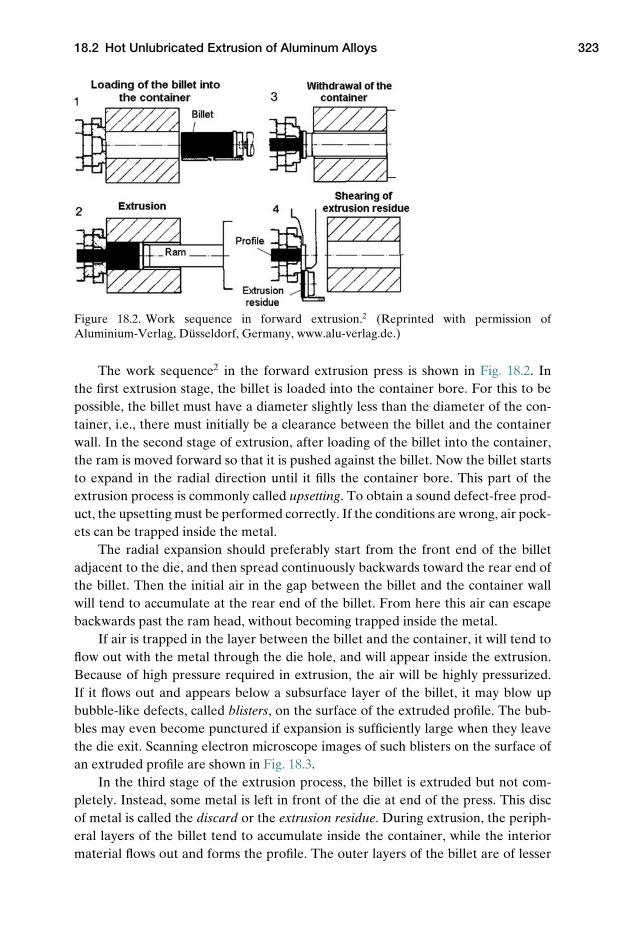
18.2 Hot Unlubricated Extrusion of Aluminum Alloys 323
Figure 18.2. Work sequence in forward extrusion.2 (Reprinted with permission ofAluminium-Verlag, Dusseldorf, Germany, www.alu-verlag.de.)
The work sequence2 in the forward extrusion press is shown in Fig. 18.2. Inthe first extrusion stage, the billet is loaded into the container bore. For this to bepossible, the billet must have a diameter slightly less than the diameter of the con-tainer, i.e., there must initially be a clearance between the billet and the containerwall. In the second stage of extrusion, after loading of the billet into the container,the ram is moved forward so that it is pushed against the billet. Now the billet startsto expand in the radial direction until it fills the container bore. This part of theextrusion process is commonly called upsetting. To obtain a sound defect-free prod-uct, the upsetting must be performed correctly. If the conditions are wrong, air pock-ets can be trapped inside the metal.
The radial expansion should preferably start from the front end of the billetadjacent to the die, and then spread continuously backwards toward the rear end ofthe billet. Then the initial air in the gap between the billet and the container wallwill tend to accumulate at the rear end of the billet. From here this air can escapebackwards past the ram head, without becoming trapped inside the metal.
If air is trapped in the layer between the billet and the container, it will tend toflow out with the metal through the die hole, and will appear inside the extrusion.Because of high pressure required in extrusion, the air will be highly pressurized.If it flows out and appears below a subsurface layer of the billet, it may blow upbubble-like defects, called blisters, on the surface of the extruded profile. The bub-bles may even become punctured if expansion is sufficiently large when they leavethe die exit. Scanning electron microscope images of such blisters on the surface ofan extruded profile are shown in Fig. 18.3.
In the third stage of the extrusion process, the billet is extruded but not com-pletely. Instead, some metal is left in front of the die at end of the press. This discof metal is called the discard or the extrusion residue. During extrusion, the periph-eral layers of the billet tend to accumulate inside the container, while the interiormaterial flows out and forms the profile. The outer layers of the billet are of lesser
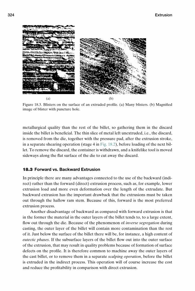
324 Extrusion
(a) (b)
Figure 18.3. Blisters on the surface of an extruded profile. (a) Many blisters. (b) Magnifiedimage of blister with puncture hole.
metallurgical quality than the rest of the billet, so gathering them in the discardinside the billet is beneficial. The thin slice of metal left unextruded, i.e., the discard,is removed from the die, together with the pressure pad, after the extrusion stroke,in a separate shearing operation (stage 4 in Fig. 18.2), before loading of the next bil-let. To remove the discard, the container is withdrawn, and a knifelike tool is movedsideways along the flat surface of the die to cut away the discard.
18.3 Forward vs. Backward Extrusion
In principle there are many advantages connected to the use of the backward (indi-rect) rather than the forward (direct) extrusion process, such as, for example, lowerextrusion load and more even deformation over the length of the extrudate. Butbackward extrusion has the important drawback that the extrusions must be takenout through the hallow ram stem. Because of this, forward is the most preferredextrusion process.
Another disadvantage of backward as compared with forward extrusion is thatin the former the material in the outer layers of the billet tends to, to a large extent,flow out through the die. Because of the phenomenon of inverse segregation duringcasting, the outer layer of the billet will contain more contamination than the restof it. Just below the surface of the billet there will be, for instance, a high content ofeutectic phases. If the subsurface layers of the billet flow out into the outer surfaceof the extrusion, that may result in quality problems because of formation of surfacedefects on the profile. It is therefore common to machine away the outer layers ofthe cast billet, or to remove them in a separate scalping operation, before the billetis extruded in the indirect process. This operation will of course increase the costand reduce the profitability in comparison with direct extrusion.
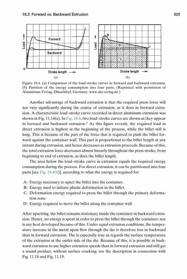
18.3 Forward vs. Backward Extrusion 325
(a) (b)
Figure 18.4. (a) Comparison of the load–stroke curves in forward and backward extrusion.(b) Partition of the energy consumption into four parts. (Reprinted with permission ofAluminium-Verlag, Dusseldorf, Germany, www.alu-verlag.de.)
Another advantage of backward extrusion is that the required press force willnot vary significantly during the course of extrusion, as it does in forward extru-sion. A characteristic load–stroke curve recorded in direct aluminum extrusion wasshown in Fig. 11.14(a). In Fig. 18.4, two load–stroke curves are shown as they appearin forward and backward extrusion.2 As this figure reveals, the required load indirect extrusion is highest in the beginning of the process, while the billet still islong. This is because of the part of the force that is required to push the billet for-ward against the container wall. This part is proportional to the billet length at anyinstant during extrusion, and hence decreases as extrusion proceeds. Because of this,the total extrusion force decreases almost linearly throughout the press stroke, frombeginning to end of extrusion, as does the billet length.
The area below the load–stroke curve in extrusion equals the required energyconsumption during the process. For direct extrusion, it can be partitioned into fourparts [see Fig. 18.4(b)], according to what the energy is required for:
A: Energy necessary to upset the billet into the container.B: Energy used to initiate plastic deformation in the billet.C: Deformation energy required to press the billet through the primary deforma-
tion zone.D: Energy required to move the billet along the container wall.
After upsetting, the billet remains stationary inside the container in backward extru-sion. Hence, no energy is spent in order to press the billet through the container; noris any heat developed because of this. Under equal extrusion conditions, the temper-ature increase in the metal upon flow through the die is therefore less in backwardthan in forward extrusion. The is especially true as regards the surface temperatureof the extrusion at the outlet side of the die. Because of this, it is possible in back-ward extrusion to use higher extrusion speeds than in forward extrusion and still geta sound product, without surface cracking; see the description in connection withFig. 11.18 and Fig. 11.19.
326 Extrusion
In spite of all the mentioned advantages of backward extrusion, it is the forwardextrusion process that has gained the most widespread use. The primary reason forthis is that it is difficult, in backward extrusion, to take the extruded profile outthrough the hollow stem construction, especially when many profiles are extrudedconcurrently, as is done in multihole extrusion. Backward extrusion is thereforerather seldom applied in industry, and when used, it is primarily for extrusion ofprofiles of simple shape.
18.4 Classification of Metal Flow in Extrusion
Material flow in metal extrusion can be quite complex and can differ considerablyfor different metals. It was therefore early considered useful to establish a classifica-tion system describing the different types of flow observed. Even for a specific metalalloy, the metal flow can vary if the friction over the boundary interface between thebillet and the die or container is altered, for instance, by use of lubrication. Further-more, characteristic flow-related extrusion defects occurring in metal extrusion canbe explained and understood on the basis of different types of flow patterns.
The most commonly used classification system today – the one proposed byPearson and Parkins3 and by Durrschnabel4 – refers to extrusion through flat-faceddies. This classification system divides metal flow in axisymmetric extrusion into fourdifferent classes, flow patterns S, A, B, and C. Use of grid patterns for metal flowanalysis has already been explained in Ch. 12.
Metal flow in unlubricated hot extrusion of aluminum or aluminum alloysthrough flat-faced dies does not correspond well to any of the flow patterns orig-inally proposed. Therefore, a modified classification system has also been proposed,with particular adaptation to aluminum extrusion5; see Fig. 18.5. In this system, twonew intermediate flow patterns A1 and B1 are added. In the new system, metal flowin indirect extrusion conforms to flow pattern A1, and metal flow in direct extrusionconforms to flow pattern B1.
If a metal flows in accordance with flow pattern B, in its natural unlubricatedcondition, a continuous change in metal flow in the direction B → A → S can occurfor this material, if friction at the interface between the billet and the die, includingthat at the container wall, is gradually reduced by the introduction of lubricants ofincreasing lubricity. The various flow patterns are as follows:
Flow pattern S: This pattern occurs characteristically when a billet with uniformflow stress over the cross section is extruded with low friction against the billetand the container wall, including the die. With sufficiently low friction, therewill be complete sliding at these interfaces during extrusion. Then the periph-eral layers of the billet will flow along the die faces and through the die holeslightly later than the core of the billet. This is easily seen by observing theappearance of the radial lines of the grid pattern for flow type S in Fig. 18.5.
Flow pattern A: This flow pattern occurs for a billet with uniform flow stressover the cross section if there is sticking friction along the die–billet interface,
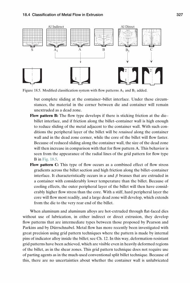
18.4 Classification of Metal Flow in Extrusion 327
S
Al Indirect
A1 A
1 1
2 2
B
Al Direct
B1 C
Figure 18.5. Modified classification system with flow patterns A1 and B1 added.
but complete sliding at the container–billet interface. Under these circum-stances, the material in the corner between die and container will remainunextruded as a dead zone.
Flow pattern B: The flow type develops if there is sticking friction at the die–billet interface, and if friction along the billet–container wall is high enoughto reduce sliding of the metal adjacent to the container wall. With such con-ditions the peripheral layer of the billet will be retained along the containerwall and in the dead zone corner, while the core of the billet will flow faster.Because of reduced sliding along the container wall, the size of the dead zonewill then increase in comparison with that for flow pattern A. This behavior isseen from the appearance of the radial lines of the grid pattern for flow typeB in Fig. 18.5.
Flow pattern C: This type of flow occurs as a combined effect of flow stressgradients across the billet section and high friction along the billet–containerinterface. It characteristically occurs in α and β brasses that are extruded ina container with considerably lower temperature than the billet. Because ofcooling effects, the outer peripheral layer of the billet will then have consid-erably higher flow stress than the core. With a stiff, hard peripheral layer thecore will flow most readily, and a large dead zone will develop, which extendsfrom the die to the very rear end of the billet.
When aluminum and aluminum alloys are hot-extruded through flat-faced dieswithout use of lubrication, in either indirect or direct extrusion, they developflow patterns that are intermediate types between those proposed by Pearson andParkins and by Durrschnabel. Metal flow has more recently been investigated withgreat precision using grid pattern techniques where the pattern is made by internalpins of indicator alloy inside the billet; see Ch. 12. In this way, deformation-resistantgrid patterns have been achieved, which are visible even in heavily deformed regionsof the billet, as in the shear zones. This grid pattern technique does not require useof parting agents as in the much-used conventional split billet technique. Because ofthis, there are no uncertainties about whether the container wall is unlubricated
328 Extrusion
when this technique is used. A special extrusion and removal technique has alsobeen developed that allows partially extruded billets to be removed from the con-tainer without plastic deformation during removal; see Fig. 19.2. In this manner,perfect grid patterns have been achieved, which map the frozen deformation condi-tion of the billet when extrusion is stopped; see Fig. 12.4.
In view of the more recent investigations, two new, intermediate flow patternscharacterizing indirect and direct extrusion can be added to the classification systemproposed by Pearson and Parkins and by Durrschnabel. It is proposed to term theseflow patterns A1 and B1; see Fig. 18.5. Pattern A1 is intermediate between patternsS and A, and pattern B1 is intermediate between patterns B and C.
Flow pattern B1: This flow pattern (see Fig. 18.5) is characterized by completesticking between the billet and the container wall or die. Because of this, theperipheral skin – including a subsurface layer of the billet – remains at thecontainer wall and is scraped off by the advancing ram during the course ofextrusion. This material therefore gathers in the rear corner of the billet,where it first flows radially inwards, and thereafter in the extrusion direction.Because of this, the material in the rear end of the billet is subjected to a grad-ual predeformation throughout the extrusion stroke, prior to its arrival intothe primary deformation zone above the die hole. Except for this additionalflow in the rear end of the billet, the flow in direct extrusion of aluminumdoes not deviate much from that previously described for flow pattern B.However, an exception is that the shear zone becomes more developed andextends deeper into the rear end of the billet. The shear zone forms betweenthe stationary layer of material at the container wall and in the dead zoneand the core of the billet which flows forward past the stationary material,toward the die opening.
Flow pattern A1: Metal flow in unlubricated indirect extrusion deviates con-siderably from that in direct extrusion, because of the stationary conditionof the billet material inside the container. Deformation occurs as the die ispushed into the billet. Because there is sticking friction between the periph-eral layer of the billet and the container wall, this layer is scraped off fromthe container wall by the advancing die, in a way similar to the scraping bythe ram at the rear billet end in direct extrusion. Because of the scrapingaction of the die against the container wall, no dead zone corresponding tothat in direct extrusion forms. However, a thin initial metal layer adjacent tothe flat-faced die will remain there during extrusion and will become heav-ily deformed by the strong metal flow deeper inside the billet material. Thislayer will be contained in the shear zone, where it is subjected to heavy defor-mations but will remain unextruded because it is located so close to the die.Moreover, because of the mentioned flow phenomenon in the corner betweenthe die and the container, the radial lines of the grid pattern will show aconvex curvature adjacent to the die, instead of concave shape as in directextrusion.
18.5 Outflow of the Outer Layers and the Skin of the Billet 329
18.5 Outflow of the Outer Layers and the Skin of the Billet
As explained in the preceding section, different flow types occur in extrusion dueto different friction conditions at the interface between the billet and the containerwall and die. Because of cooling effects, the outer layers of the billet can have higherflow stress than the interior of the billet. Then there is even stronger retention ofthe peripheral layer of the billet, and this will make the billet flow according to flowtype C.
The tendency of outflow of the peripheral skin of the billet and the subsurfacelayers below the skin into the extrusion is therefore uniquely determined by theflow pattern, as depicted in Fig. 18.5, where the subsurface layers have been paintedblack.
18.5.1 Flow Pattern S
When the billet flows according to flow type S, the billet skin and the material belowwill slide along the container wall and the die. At a certain stage of extrusion, theywill start to flow out of the die opening, into the extrusion. Here they will appearon the surface of the extrusion; see Fig. 18.5. Hence, when steady-state conditionshave been reached in the extrusion process, the outer skin of the extrusion will orig-inate from the billet skin. In addition, a subsurface layer of given thickness from theas-cast billet will appear as a subsurface layer in the final extrusion. In the extru-date, this layer will have approximately constant thickness when the steady-statecondition has been reached.
18.5.2 Flow Patterns A, A1, and B
Because of partial or complete sticking at the interface between the billet and thedie or container wall, some material initially in the front end of the billet will remainstagnant in the front end during extrusion, either in the dead zone adjacent to thedie, or in the shear zone.
With some sliding at the container wall, as experienced for flow types A and B,the billet skin – including the subsurface layers below the skin – will flow into theinterior of the billet, on top of the stagnant material in the dead zone and in theshear zone; see Fig. 18.5. This material will flow slowly forward until it flows out ofthe die hole and into the extrusion, where it will appear as a subsurface layer.
Because of the deformation in the shear zone, a thin layer of material is con-currently fed out gradually from the shear zone into the very outer surface layer ofthe extrusion. This material will cover the sublayer created from the outer layers ofthe billet and will also generate the new surface skin that is formed on the extru-sion. The small region inside the billet that feeds this material forward was shown inFig. 12.9(b), and can preferably be termed the slow flowing zone.
If the initial billet skin overfolds on top of the dead zone and flows into thesubcutaneous layers of the extrusion, it will appear as an extrusion defect, commonly
330 Extrusion
called scaling. Depending on the nature of the initial oxide film on the surface of thebillet and an eventual lubrication following the film, the metal layer flowing from theslow flowing zone, appearing on top of the initial billet skin, may behave differently.It can either partially pressure-weld onto the billet skin or, in case of poor welding,be pulled off from the extrudate as a loose scale. The process of inward flow of theinitial peripheral skin of the billet on top of the dead zone into the extrusion can becompared with the well-known phenomenon of overfolding sometimes taking placein forging; see Fig. 16.10. In forging, the phenomenon is known to cause materialdefects like laps or cold shuts.
When the overfolding occurs, i.e., whether it occurs early or late during extru-sion, depends on two factors. These are the degree of slipping at the container wall,and the size of the flat-faced portion of the die on which the dead zone rests. Withincreased slipping, i.e., with reduced friction along the billet–container interface,the peripheral layer and the billet skin tend to flow into the extrusion at an earlierstage. The same happens if the die hole is moved closer to the container wall. Thena smaller dead zone forms, and the flow path of the skin and peripheral subsurfacelayer of the billet, on top of the dead zone and the slow flowing zone, into the extru-sion becomes shorter.
In unlubricated indirect extrusion of aluminum, i.e., for flow pattern A1, thereis complete sticking in the boundary layer between the billet and the container wall.The billet skin then sticks to the container and does not flow on top of the materialfrom the dead zone and the slow flowing zone. However, the thin subsurface periph-eral layer of the billet will still flow that way and will finally appear right under thesurface of the extrusion. If this layer contains contamination, it can cause surfacequality problems in the extrusion process. If no lubrication is used in the extrusionprocess, the surface skin of the billet will accumulate in the billet discard and willnot flow into the extrusion. This is advantageous in that the billet skin then will bepresent in the final metal residue, which is discarded after the end of each presscycle.
18.5.3 Flow Pattern B1
For this flow type, the inward flow of the peripheral billet layer on top of the deadzone and into the profile will occur in the same way as described previously for flowtypes A1, A, and B; see Fig. 18.5. Now, however, this flow will be delayed, becausethe retention of the peripheral layer of the billet is stronger than for the other flowtypes. Because of sticking friction along the container wall and the die, the skinof the billet will not flow into the extrusion, unless traces of lubricant are present onthe billet skin or on the container wall.
Because of the previously mentioned scraping off of the adhering peripheralbillet layer as the ram advances down along the container wall, and the packing ofthis layer radially inwards into the rear end of the billet, this material will tend toflow inwards into the rear end of the billet; see Fig. 18.5. Hence, for this flow type,
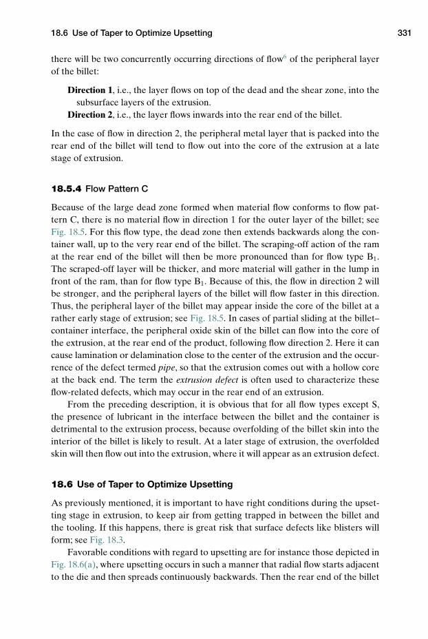
18.6 Use of Taper to Optimize Upsetting 331
there will be two concurrently occurring directions of flow6 of the peripheral layerof the billet:
Direction 1, i.e., the layer flows on top of the dead and the shear zone, into thesubsurface layers of the extrusion.
Direction 2, i.e., the layer flows inwards into the rear end of the billet.
In the case of flow in direction 2, the peripheral metal layer that is packed into therear end of the billet will tend to flow out into the core of the extrusion at a latestage of extrusion.
18.5.4 Flow Pattern C
Because of the large dead zone formed when material flow conforms to flow pat-tern C, there is no material flow in direction 1 for the outer layer of the billet; seeFig. 18.5. For this flow type, the dead zone then extends backwards along the con-tainer wall, up to the very rear end of the billet. The scraping-off action of the ramat the rear end of the billet will then be more pronounced than for flow type B1.The scraped-off layer will be thicker, and more material will gather in the lump infront of the ram, than for flow type B1. Because of this, the flow in direction 2 willbe stronger, and the peripheral layers of the billet will flow faster in this direction.Thus, the peripheral layer of the billet may appear inside the core of the billet at arather early stage of extrusion; see Fig. 18.5. In cases of partial sliding at the billet–container interface, the peripheral oxide skin of the billet can flow into the core ofthe extrusion, at the rear end of the product, following flow direction 2. Here it cancause lamination or delamination close to the center of the extrusion and the occur-rence of the defect termed pipe, so that the extrusion comes out with a hollow coreat the back end. The term the extrusion defect is often used to characterize theseflow-related defects, which may occur in the rear end of an extrusion.
From the preceding description, it is obvious that for all flow types except S,the presence of lubricant in the interface between the billet and the container isdetrimental to the extrusion process, because overfolding of the billet skin into theinterior of the billet is likely to result. At a later stage of extrusion, the overfoldedskin will then flow out into the extrusion, where it will appear as an extrusion defect.
18.6 Use of Taper to Optimize Upsetting
As previously mentioned, it is important to have right conditions during the upset-ting stage in extrusion, to keep air from getting trapped in between the billet andthe tooling. If this happens, there is great risk that surface defects like blisters willform; see Fig. 18.3.
Favorable conditions with regard to upsetting are for instance those depicted inFig. 18.6(a), where upsetting occurs in such a manner that radial flow starts adjacentto the die and then spreads continuously backwards. Then the rear end of the billet
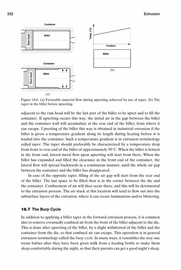
332 Extrusion
(a)
(b)
Figure 18.6. (a) Favorable material flow during upsetting achieved by use of taper. (b) Thetaper in the billet before upsetting.
adjacent to the ram head will be the last part of the billet to be upset and to fill thecontainer. If upsetting occurs this way, the initial air in the gap between the billetand the container wall will accumulate at the rear end of the billet, from where itcan escape. Upsetting of the billet this way is obtained in industrial extrusion if thebillet is given a temperature gradient along its length during heating before it isloaded into the container. Such a temperature gradient is in extrusion terminologycalled taper. The taper should preferably be characterized by a temperature dropfrom front to rear end of the billet of approximately 50◦C. When the billet is hottestin the front end, lateral metal flow upon upsetting will start from there. When thebillet has expanded and filled the clearance in the front end of the container, thelateral flow will spread backwards in a continuous manner, until the whole air gapbetween the container and the billet has disappeared.
In case of the opposite taper, filling of the air gap will start from the rear endof the billet. The last space to be filled then is in the corner between the die andthe container. Confinement of air will then occur there, and this will be detrimentalto the extrusion process. The air stuck at this location will tend to flow out into thesubsurface layers of the extrusion, where it can create laminations and/or blistering.
18.7 The Burp Cycle
In addition to applying a billet taper in the forward extrusion process, it is commonalso to remove eventually confined air from the front of the billet adjacent to the die.This is done after upsetting of the billet, by a slight withdrawal of the billet and thecontainer from the die, so that confined air can escape. This operation is in generalextrusion terminology called the burp cycle. In many ways, it resembles the way onetreats babies after they have been given milk from a feeding bottle to make themsleep comfortably during the night, so that their parents can get a good night’s sleep.
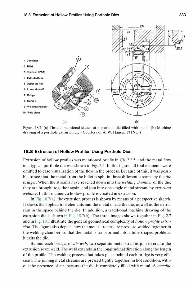
18.8 Extrusion of Hollow Profiles Using Porthole Dies 333
(a) (b)
Figure 18.7. (a) Three-dimensional sketch of a porthole die filled with metal. (b) Machinedrawing of a porthole extrusion die. (Courtesy of A. W. Hansen, NTNU.)
18.8 Extrusion of Hollow Profiles Using Porthole Dies
Extrusion of hollow profiles was mentioned briefly in Ch. 2.2.5, and the metal flowin a typical porthole die was shown in Fig. 2.5. In this figure, all tool elements wereomitted to ease visualization of the flow in the process. Because of this, it was possi-ble to see that the metal from the billet is split in three different streams by the diebridges. When the streams have reached down into the welding chamber of the die,they are brought together again, and join into one single metal stream, by extrusionwelding. In this manner, a hollow profile is created in extrusion.
In Fig. 18.7(a), the extrusion process is shown by means of a perspective sketch.It shows the applied tool elements and the metal inside the die, as well as the extru-sion in the space behind the die. In addition, a traditional machine drawing of theextrusion die is shown in Fig. 18.7(b). The three images shown together in Fig. 2.7and in Fig. 18.7 illustrate the general geometrical complexity of hollow profile extru-sion. The figure also depicts how the metal streams are pressure-welded together inthe welding chamber, so that the metal is transformed into a tube-shaped profile asit exits the die.
Behind each bridge, or die web, two separate metal streams join to create theextrusion seam weld. The weld extends in the longitudinal direction along the lengthof the profile. The welding process that takes place behind each bridge is very effi-cient. The joining metal streams are pressed tightly together, in hot condition, with-out the presence of air, because the die is completely filled with metal. A metallic
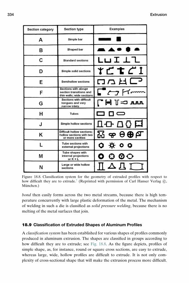
334 Extrusion
Figure 18.8. Classification system for the geometry of extruded profiles with respect tohow difficult they are to extrude.7 (Reprinted with permission of Carl Hanser Verlag c©,Munchen.)
bond then easily forms across the two metal streams, because there is high tem-perature concurrently with large plastic deformation of the metal. The mechanismof welding in such a die is classified as solid pressure welding, because there is nomelting of the metal surfaces that join.
18.9 Classification of Extruded Shapes of Aluminum Profiles
A classification system has been established for various shapes of profiles commonlyproduced in aluminum extrusion. The shapes are classified in groups according tohow difficult they are to extrude; see Fig. 18.8. As the figure depicts, profiles ofsimple shape, as, for instance, round or square cross sections, are easy to extrude,whereas large, wide, hollow profiles are difficult to extrude. It is not only com-plexity of cross-sectional shape that will make the extrusion process more difficult.
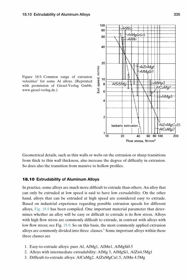
18.10 Extrudability of Aluminum Alloys 335
Figure 18.9. Common range of extrusionvelocities8 for some Al alloys. (Reprintedwith permission of Giesel-Verlag Gmbh;www.giesel-verlag.de.)
Geometrical details, such as thin walls or webs on the extrusion or sharp transitionsfrom thick to thin wall thickness, also increase the degree of difficulty in extrusion.So does also the transition from massive to hollow profiles.
18.10 Extrudability of Aluminum Alloys
In practice, some alloys are much more difficult to extrude than others. An alloy thatcan only be extruded at low speed is said to have low extrudability. On the otherhand, alloys that can be extruded at high speed are considered easy to extrude.Based on industrial experience regarding possible extrusion speeds for differentalloys, Fig. 18.9 has been compiled. One important material parameter that deter-mines whether an alloy will be easy or difficult to extrude is its flow stress. Alloyswith high flow stress are commonly difficult to extrude, in contrast with alloys withlow flow stress; see Fig. 18.9. So on this basis, the most commonly applied extrusionalloys are commonly divided into three classes.8 Some important alloys within thesethree classes are
1. Easy-to-extrude alloys: pure Al, AlMg1, AlMn1, AlMgSi0.52. Alloys with intermediate extrudability: AlMg 3, AlMgSi1, AlZn4.5Mg13. Difficult-to-extrude alloys: AlCuMg2, AlZnMgCu1.5, AlMn 4.5Mg
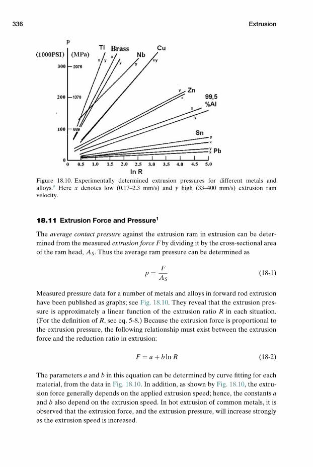
336 Extrusion
Figure 18.10. Experimentally determined extrusion pressures for different metals andalloys.9 Here x denotes low (0.17–2.3 mm/s) and y high (33–400 mm/s) extrusion ramvelocity.
18.11 Extrusion Force and Pressure1
The average contact pressure against the extrusion ram in extrusion can be deter-mined from the measured extrusion force F by dividing it by the cross-sectional areaof the ram head, AS. Thus the average ram pressure can be determined as
p = FAS
(18-1)
Measured pressure data for a number of metals and alloys in forward rod extrusionhave been published as graphs; see Fig. 18.10. They reveal that the extrusion pres-sure is approximately a linear function of the extrusion ratio R in each situation.(For the definition of R, see eq. 5-8.) Because the extrusion force is proportional tothe extrusion pressure, the following relationship must exist between the extrusionforce and the reduction ratio in extrusion:
F = a + b ln R (18-2)
The parameters a and b in this equation can be determined by curve fitting for eachmaterial, from the data in Fig. 18.10. In addition, as shown by Fig. 18.10, the extru-sion force generally depends on the applied extrusion speed; hence, the constants aand b also depend on the extrusion speed. In hot extrusion of common metals, it isobserved that the extrusion force, and the extrusion pressure, will increase stronglyas the extrusion speed is increased.
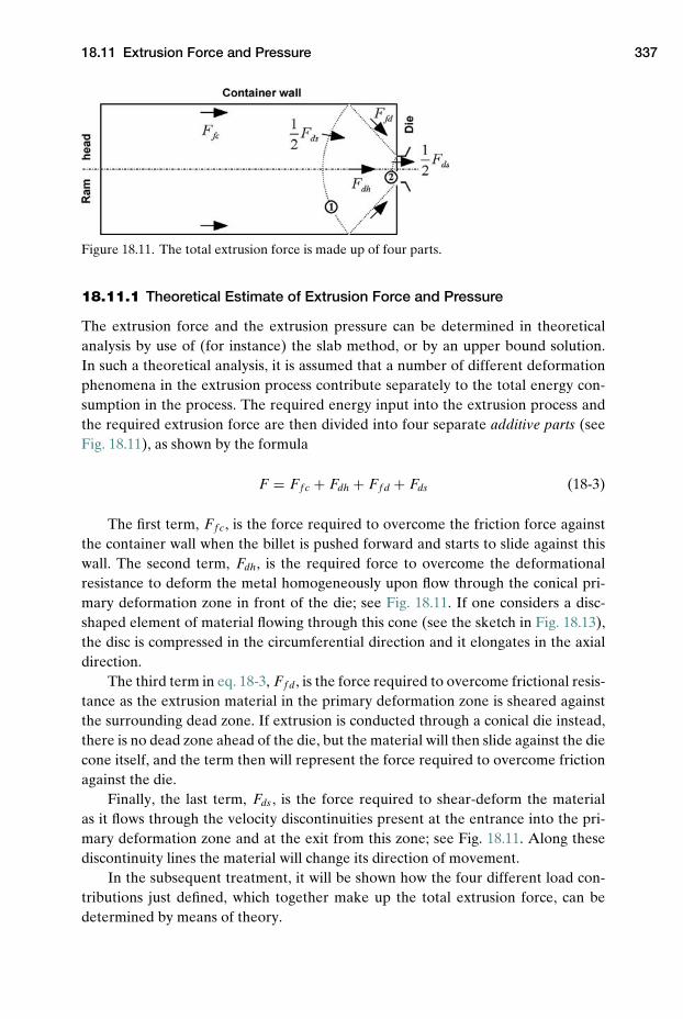
18.11 Extrusion Force and Pressure 337
Figure 18.11. The total extrusion force is made up of four parts.
18.11.1 Theoretical Estimate of Extrusion Force and Pressure
The extrusion force and the extrusion pressure can be determined in theoreticalanalysis by use of (for instance) the slab method, or by an upper bound solution.In such a theoretical analysis, it is assumed that a number of different deformationphenomena in the extrusion process contribute separately to the total energy con-sumption in the process. The required energy input into the extrusion process andthe required extrusion force are then divided into four separate additive parts (seeFig. 18.11), as shown by the formula
F = Ff c + Fdh + Ff d + Fds (18-3)
The first term, Ff c, is the force required to overcome the friction force againstthe container wall when the billet is pushed forward and starts to slide against thiswall. The second term, Fdh, is the required force to overcome the deformationalresistance to deform the metal homogeneously upon flow through the conical pri-mary deformation zone in front of the die; see Fig. 18.11. If one considers a disc-shaped element of material flowing through this cone (see the sketch in Fig. 18.13),the disc is compressed in the circumferential direction and it elongates in the axialdirection.
The third term in eq. 18-3, Ff d, is the force required to overcome frictional resis-tance as the extrusion material in the primary deformation zone is sheared againstthe surrounding dead zone. If extrusion is conducted through a conical die instead,there is no dead zone ahead of the die, but the material will then slide against the diecone itself, and the term then will represent the force required to overcome frictionagainst the die.
Finally, the last term, Fds , is the force required to shear-deform the materialas it flows through the velocity discontinuities present at the entrance into the pri-mary deformation zone and at the exit from this zone; see Fig. 18.11. Along thesediscontinuity lines the material will change its direction of movement.
In the subsequent treatment, it will be shown how the four different load con-tributions just defined, which together make up the total extrusion force, can bedetermined by means of theory.
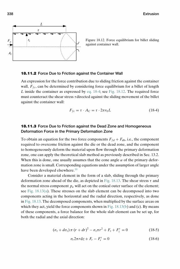
338 Extrusion
Figure 18.12. Force equilibrium for billet slidingagainst container wall.
18.11.2 Force Due to Friction against the Container Wall
An expression for the force contribution due to sliding friction against the containerwall, Ff c, can be determined by considering force equilibrium for a billet of lengthL inside the container as expressed by eq. 18-4; see Fig. 18.12. The required forcemust counteract the shear stress τdirected against the sliding movement of the billetagainst the container wall:
Ff c = τ · AC = τ · 2πr0L (18-4)
18.11.3 Force Due to Friction against the Dead Zone and HomogeneousDeformation Force in the Primary Deformation Zone
To obtain an equation for the two force components Ff d + Fdh, i.e., the componentrequired to overcome friction against the die or the dead zone, and the componentto homogeneously deform the material upon flow through the primary deformationzone, one can apply the theoretical slab method as previously described in Sec. 13.2.When this is done, one usually assumes that the cone angle α of the primary defor-mation zone is small. Corresponding equations under the assumption of larger anglehave been developed elsewhere.10
Consider a material element in the form of a slab, sliding through the primarydeformation zone ahead of the die, as depicted in Fig. 18.13. The shear stress τ andthe normal stress component pα will act on the conical outer surface of the element;see Fig. 18.13(a). These stresses on the slab element can be decomposed into twocomponents acting in the horizontal and the radial direction, respectively, as donein Fig. 18.13. The decomposed components, when multiplied by the surface areas onwhich they act, yield the force components shown in Fig. 18.13(b) and (c). By meansof these components, a force balance for the whole slab element can be set up, forboth the radial and the axial direction:
(σz + dσz) π (r + dr)2 − σzπr2 + Fz + F τz = 0 (18-5)
σr 2πrdz + Fr − F τr = 0 (18-6)
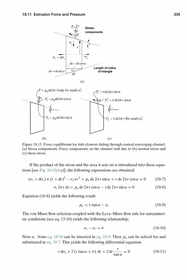
18.11 Extrusion Force and Pressure 339
(a)
(b) (c)
Figure 18.13. Force equilibrium for slab element sliding through conical converging channel.(a) Stress components. Force components on the channel wall due to (b) normal stress and(c) shear stress.
If the product of the stress and the area it acts on is introduced into these equa-tions [see Fig. 18.13(b,c)], the following expressions are obtained:
(σz + dσz) π (r + dr)2 − σzπr2 + pα ds 2πr sin α + τ ds 2πr cos α = 0 (18-7)
σr 2πr dz + pα ds 2πr cos α − τds 2πr sin α = 0 (18-8)
Equation (18-8) yields the following result:
pα = τ tan α − σr (18-9)
The von Mises flow criterion coupled with the Levy–Mises flow rule for axisymmet-ric conditions (see eq. 13-10) yields the following relationship:
σz − σr = σ (18-10)
Now σr from eq. 18-10 can be inserted in eq. 18-9. Then pα can be solved for andsubstituted in eq. 18-7. This yields the following differential equation:
r dσz + 2 (τ tan α + σ ) dr + 2 drτ
tan α= 0 (18-11)
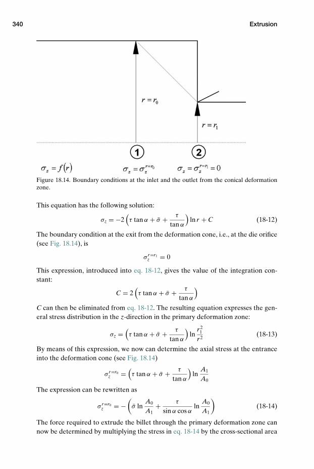
340 Extrusion
Figure 18.14. Boundary conditions at the inlet and the outlet from the conical deformationzone.
This equation has the following solution:
σz = −2(τ tan α + σ + τ
tan α
)ln r + C (18-12)
The boundary condition at the exit from the deformation cone, i.e., at the die orifice(see Fig. 18.14), is
σ r=r1z = 0
This expression, introduced into eq. 18-12, gives the value of the integration con-stant:
C = 2(τ tan α + σ + τ
tan α
)C can then be eliminated from eq. 18-12. The resulting equation expresses the gen-eral stress distribution in the z-direction in the primary deformation zone:
σz =(τ tan α + σ + τ
tan α
)ln
r21
r2(18-13)
By means of this expression, we now can determine the axial stress at the entranceinto the deformation cone (see Fig. 18.14)
σ r=r0z =
(τ tan α + σ + τ
tan α
)ln
A1
A0
The expression can be rewritten as
σ r=r0z = −
(σ ln
A0
A1+ τ
sin α cos αln
A0
A1
)(18-14)
The force required to extrude the billet through the primary deformation zone cannow be determined by multiplying the stress in eq. 18-14 by the cross-sectional area
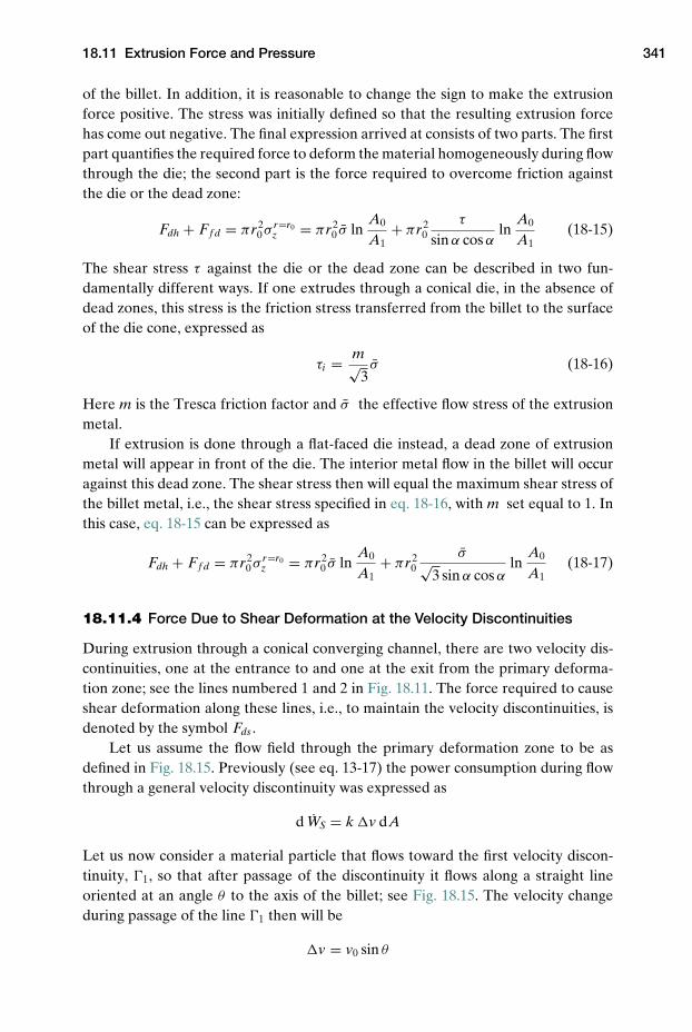
18.11 Extrusion Force and Pressure 341
of the billet. In addition, it is reasonable to change the sign to make the extrusionforce positive. The stress was initially defined so that the resulting extrusion forcehas come out negative. The final expression arrived at consists of two parts. The firstpart quantifies the required force to deform the material homogeneously during flowthrough the die; the second part is the force required to overcome friction againstthe die or the dead zone:
Fdh + Ff d = πr20 σ r=r0
z = πr20 σ ln
A0
A1+ πr2
0τ
sin α cos αln
A0
A1(18-15)
The shear stress τ against the die or the dead zone can be described in two fun-damentally different ways. If one extrudes through a conical die, in the absence ofdead zones, this stress is the friction stress transferred from the billet to the surfaceof the die cone, expressed as
τi = m√3σ (18-16)
Here m is the Tresca friction factor and σ the effective flow stress of the extrusionmetal.
If extrusion is done through a flat-faced die instead, a dead zone of extrusionmetal will appear in front of the die. The interior metal flow in the billet will occuragainst this dead zone. The shear stress then will equal the maximum shear stress ofthe billet metal, i.e., the shear stress specified in eq. 18-16, with m set equal to 1. Inthis case, eq. 18-15 can be expressed as
Fdh + Ff d = πr20 σ r=r0
z = πr20 σ ln
A0
A1+ πr2
0σ√
3 sin α cos αln
A0
A1(18-17)
18.11.4 Force Due to Shear Deformation at the Velocity Discontinuities
During extrusion through a conical converging channel, there are two velocity dis-continuities, one at the entrance to and one at the exit from the primary deforma-tion zone; see the lines numbered 1 and 2 in Fig. 18.11. The force required to causeshear deformation along these lines, i.e., to maintain the velocity discontinuities, isdenoted by the symbol Fds .
Let us assume the flow field through the primary deformation zone to be asdefined in Fig. 18.15. Previously (see eq. 13-17) the power consumption during flowthrough a general velocity discontinuity was expressed as
d WS = k �v dA
Let us now consider a material particle that flows toward the first velocity discon-tinuity, �1, so that after passage of the discontinuity it flows along a straight lineoriented at an angle θ to the axis of the billet; see Fig. 18.15. The velocity changeduring passage of the line �1 then will be
�v = v0 sin θ
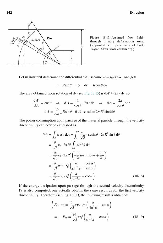
342 Extrusion
Figure 18.15. Assumed flow field1
through primary deformation zone.(Reprinted with permission of Prof.Taylan Altan. www.ercnsm.org.)
Let us now first determine the differential dA. Because R = r0/sin α, one gets
r = Rsin θ ⇒ dr = Rcos θ dθ
The area obtained upon rotation of dr (see Fig. 18.15) is dA′ ≈ 2πr dr , so
dA′
dA= cos θ ⇒ dA = 1
cos θ· 2πr dr ⇒ dA = 2π
cos θr dr
dA = 2π
cos θRsin θ · Rdθ · cos θ = 2π R2 sin θdθ
The power consumption upon passage of the material particle through the velocitydiscontinuity can now be expressed as
WS =∫
Ak �v dA =
∫ α
0
σ√3
· v0 sin θ · 2πR2 sin θ dθ
= σ√3
v0 · 2πR2∫ α
0sin2 θ dθ
= σ√3
v0 · 2πR2(
−12
sin α cos α + 12α
)
= σ√3πv0 · r2
0
(α
sin2 α− cos α
sin α
)
= σ√3πv0 · r2
0
(α
sin2 α− cot α
)(18-18)
If the energy dissipation upon passage through the second velocity discontinuity�2 is also computed, one actually obtains the same result as for the first velocitydiscontinuity. Therefore (see Fig. 18.11), the following result is obtained:
12
Fds · v0 = σ√3πv0 · r2
0
(α
sin2 α− cot α
)
⇒ Fds = 2σ√3πr2
0
(α
sin2 α− cot α
)(18-19)
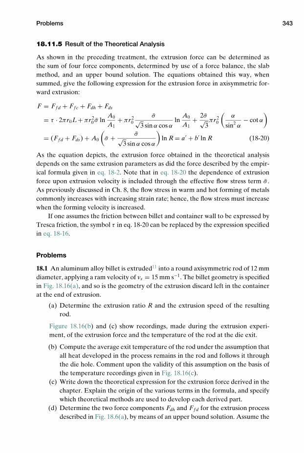
Problems 343
18.11.5 Result of the Theoretical Analysis
As shown in the preceding treatment, the extrusion force can be determined asthe sum of four force components, determined by use of a force balance, the slabmethod, and an upper bound solution. The equations obtained this way, whensummed, give the following expression for the extrusion force in axisymmetric for-ward extrusion:
F = Ff d + Ff c + Fdh + Fds
= τ · 2πr0L+ πr20 σ ln
A0
A1+ πr2
0σ√
3 sin α cos αln
A0
A1+ 2σ√
3πr2
0
(α
sin2 α− cot α
)
= (Ff d + Fds) + A0
(σ + σ√
3 sin α cos α
)ln R = a′ + b′ ln R (18-20)
As the equation depicts, the extrusion force obtained in the theoretical analysisdepends on the same extrusion parameters as did the force described by the empir-ical formula given in eq. 18-2. Note that in eq. 18-20 the dependence of extrusionforce upon extrusion velocity is included through the effective flow stress term σ .As previously discussed in Ch. 8, the flow stress in warm and hot forming of metalscommonly increases with increasing strain rate; hence, the flow stress must increasewhen the forming velocity is increased.
If one assumes the friction between billet and container wall to be expressed byTresca friction, the symbol τ in eq. 18-20 can be replaced by the expression specifiedin eq. 18-16.
Problems
18.1 An aluminum alloy billet is extruded11 into a round axisymmetric rod of 12 mmdiameter, applying a ram velocity of vs = 15 mm s−1. The billet geometry is specifiedin Fig. 18.16(a), and so is the geometry of the extrusion discard left in the containerat the end of extrusion.
(a) Determine the extrusion ratio R and the extrusion speed of the resultingrod.
Figure 18.16(b) and (c) show recordings, made during the extrusion experi-ment, of the extrusion force and the temperature of the rod at the die exit.
(b) Compute the average exit temperature of the rod under the assumption thatall heat developed in the process remains in the rod and follows it throughthe die hole. Comment upon the validity of this assumption on the basis ofthe temperature recordings given in Fig. 18.16(c).
(c) Write down the theoretical expression for the extrusion force derived in thechapter. Explain the origin of the various terms in the formula, and specifywhich theoretical methods are used to develop each derived part.
(d) Determine the two force components Fdh and Ff d for the extrusion processdescribed in Fig. 18.6(a), by means of an upper bound solution. Assume the
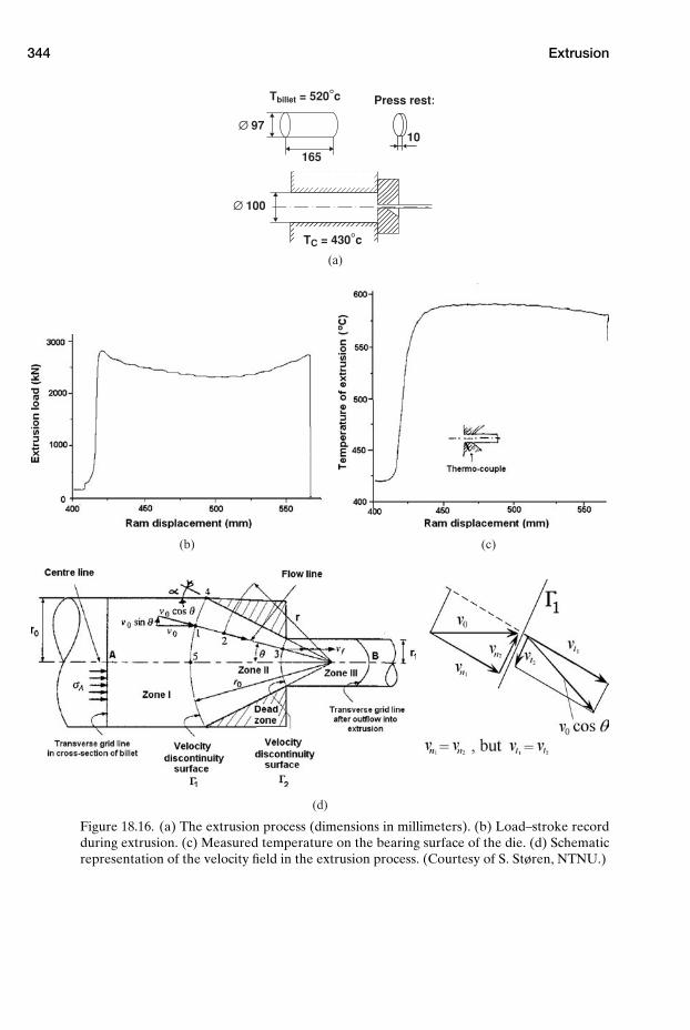
344 Extrusion
Tbillet = 520°c
TC = 430°c
Press rest:
10
165
∅ 100
∅ 97
(a)
(b) (c)
(d)
Figure 18.16. (a) The extrusion process (dimensions in millimeters). (b) Load–stroke recordduring extrusion. (c) Measured temperature on the bearing surface of the die. (d) Schematicrepresentation of the velocity field in the extrusion process. (Courtesy of S. Støren, NTNU.)
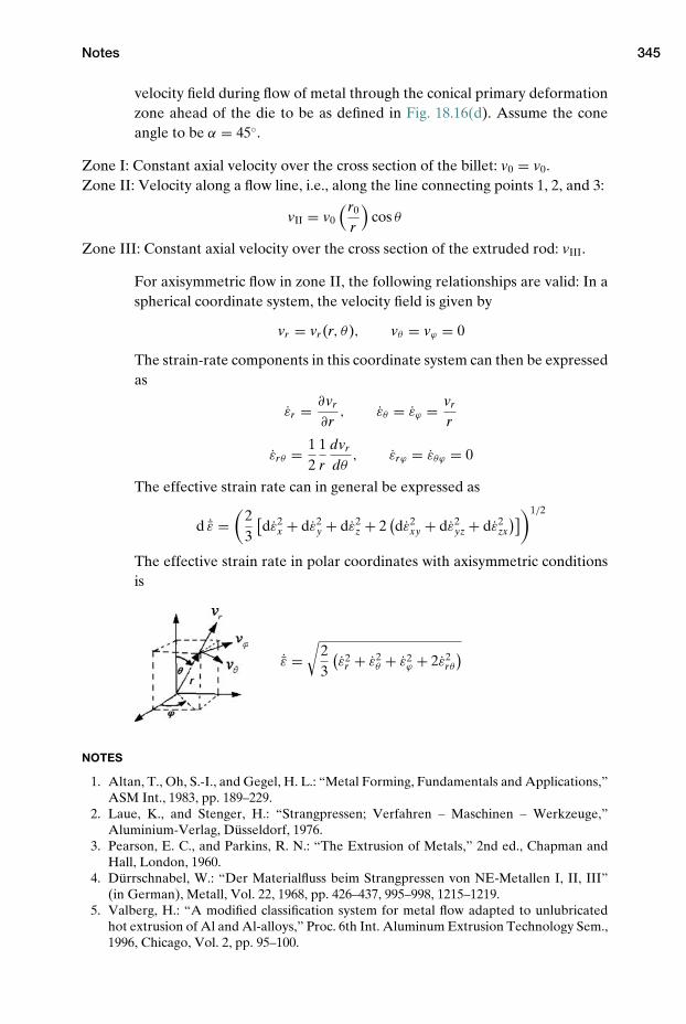
Notes 345
velocity field during flow of metal through the conical primary deformationzone ahead of the die to be as defined in Fig. 18.16(d). Assume the coneangle to be α = 45◦.
Zone I: Constant axial velocity over the cross section of the billet: v0 = v0.Zone II: Velocity along a flow line, i.e., along the line connecting points 1, 2, and 3:
vII = v0
(r0
r
)cos θ
Zone III: Constant axial velocity over the cross section of the extruded rod: vIII.
For axisymmetric flow in zone II, the following relationships are valid: In aspherical coordinate system, the velocity field is given by
vr = vr (r, θ), vθ = vϕ = 0
The strain-rate components in this coordinate system can then be expressedas
εr = ∂vr
∂r, εθ = εϕ = vr
r
εrθ = 12
1r
dvr
dθ, εrϕ = εθϕ = 0
The effective strain rate can in general be expressed as
d ˙ε =(
23
[dε2
x + dε2y + dε2
z + 2(dε2
xy + dε2yz + dε2
zx
)])1/2
The effective strain rate in polar coordinates with axisymmetric conditionsis
˙ε =√
23
(ε2
r + ε2θ + ε2
ϕ + 2ε2rθ
)
NOTES
1. Altan, T., Oh, S.-I., and Gegel, H. L.: “Metal Forming, Fundamentals and Applications,”ASM Int., 1983, pp. 189–229.
2. Laue, K., and Stenger, H.: “Strangpressen; Verfahren – Maschinen – Werkzeuge,”Aluminium-Verlag, Dusseldorf, 1976.
3. Pearson, E. C., and Parkins, R. N.: “The Extrusion of Metals,” 2nd ed., Chapman andHall, London, 1960.
4. Durrschnabel, W.: “Der Materialfluss beim Strangpressen von NE-Metallen I, II, III”(in German), Metall, Vol. 22, 1968, pp. 426–437, 995–998, 1215–1219.
5. Valberg, H.: “A modified classification system for metal flow adapted to unlubricatedhot extrusion of Al and Al-alloys,” Proc. 6th Int. Aluminum Extrusion Technology Sem.,1996, Chicago, Vol. 2, pp. 95–100.

346 Extrusion
6. Lefstad, M., Reiso, O., and Johnsen, V.: “Flow of the billet surface in aluminium extru-sion,” Proc. 5th Int. Aluminum Extrusion Technology Sem., Chicago, 1992. Vol. 2,pp. 503–517.
7. Laue, K.: “Moglichkeiten werkstoffgerechter Gestaltung von Leichtmetallprofilen,”Z. f. Metallkunde, Vol. 54, 1963, pp. 667–671.
8. Akeret, R.: “Untersuchungen uber das Strangpressen unter besonderer Beruck-sichtigung der thermischen Vorgange, Aluminium,” Vol. 44, 1968, pp. 412–415.
9. Pugh, H. L. D., and Watkins, M. T.: “Experimental Investigation of the Extrusions ofMetals,” The Inst. of Prod. Engg., Brighton, England, 1960.
10. Johnson, R. W., and Rowe, G. W.: “Redundant work in drawing cylindrical stock,”J. Inst. Metals, 1968, Vol. 96, p. 105.
11. Støren, S.: Private communication NTNU.
REFERENCES
Bauser, M., Sauer, G., and Siegert, K. (Eds.): “Extrusion,” 2nd ed., ASM Int., Metals Park,Ohio, 2006.
Laue, K., and Stenger, H.: “Extrusion,” ASM Int., Metals Park, Ohio, 1976.Saha, P. K.: “Aluminium Extrusion Technology,” ASM Int., Metals Park, Ohio, 2000.Sheppard, T.: “Extrusion of Aluminium Alloys,” Kluwer Academic Publishers, 1999.
19 FEA of Extrusion
Extrusion as a metal forming process has previously been dealt with in Sec. 2.2.5and Ch. 18. In Ch. 12, commonly used experimental grid pattern techniques weredescribed, and it was shown that such techniques are required in order to be able todescribe the deformations occurring in forward and backward extrusion. The treat-ment showed that metal flow and deformational behavior in the extrusion processesare indeed complex.
It will now be shown how simple axisymmetric aluminum extrusion can be mod-eled by FEA, with respect to both forward and backward extrusion. A compari-son of results obtained by means of simulation models with corresponding resultsfrom experimental grid pattern analysis confirms that these simulations describe thereal metal flow in extrusion with good accuracy. Finally, the FEM models are usedto show some differences in deformation characteristics in forward and backwardextrusion.
19.1 Forward Extrusion of Aluminum
19.1.1 Forward Extrusion Divided into Subprocesses
A new concept1 has been proposed to explain the complex metal flow phenom-ena taking place in the unlubricated forward extrusion process, as applied for hotextrusion of Al and Al alloys. The concept is based on considering the process to bepartitioned into four subprocesses. Then, by FEA, it is possible to model and to ana-lyze each of the four different subprocesses by individual FEM models, which eachdescribe particularly well the different deformation phenomena encountered in theforward extrusion process. The concept of division into subprocesses is useful forgaining deeper insight into the mechanics of the process. Analysis can also be doneindividually for each subprocess to optimize the complete unlubricated extrusionprocess.
The proposed principle of subdivision is shown in Fig. 19.1. The subpro-cesses, which together make up forward extrusion, are (1) shearing, (2) scratching,(3) radial compression, and (4) extrusion. In the figure, different DEFORM-2D
347
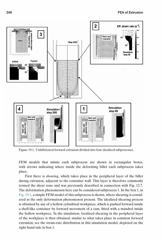
348 FEA of Extrusion
Figure 19.1. Unlubricated forward extrusion divided into four idealized subprocesses.
FEM models that mimic each subprocess are shown in rectangular boxes,with arrows indicating where inside the deforming billet each subprocess takesplace.
First there is shearing, which takes place in the peripheral layer of the billetduring extrusion, adjacent to the container wall. This layer is therefore commonlytermed the shear zone and was previously described in connection with Fig. 12.7.The deformation phenomenon here can be considered subprocess 1. In the box 1, inFig. 19.1, a simple FEM model of this subprocess is shown, where shearing is consid-ered as the only deformation phenomenon present. The idealized shearing processis obtained by use of a hollow cylindrical workpiece, which is pushed forward insidea shell-like container by forward movement of a ram, fitted with a mandrel insidethe hollow workpiece. In the simulation, localized shearing in the peripheral layerof the workpiece is then obtained, similar to what takes place in common forwardextrusion; see the strain-rate distribution in this simulation model, depicted on theright-hand side in box 1.
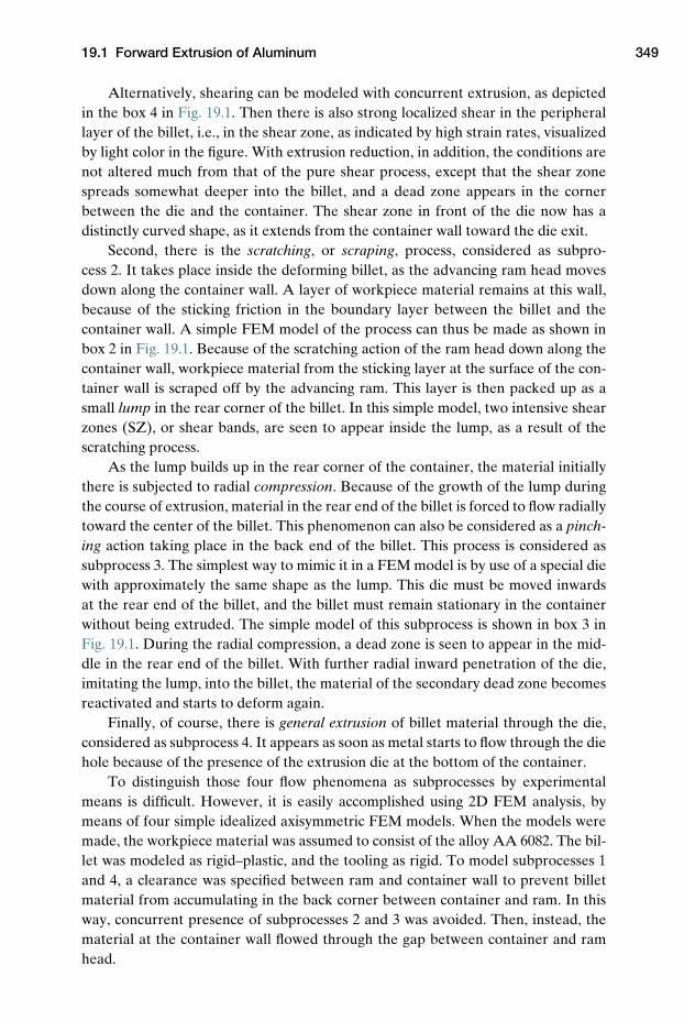
19.1 Forward Extrusion of Aluminum 349
Alternatively, shearing can be modeled with concurrent extrusion, as depictedin the box 4 in Fig. 19.1. Then there is also strong localized shear in the peripherallayer of the billet, i.e., in the shear zone, as indicated by high strain rates, visualizedby light color in the figure. With extrusion reduction, in addition, the conditions arenot altered much from that of the pure shear process, except that the shear zonespreads somewhat deeper into the billet, and a dead zone appears in the cornerbetween the die and the container. The shear zone in front of the die now has adistinctly curved shape, as it extends from the container wall toward the die exit.
Second, there is the scratching, or scraping, process, considered as subpro-cess 2. It takes place inside the deforming billet, as the advancing ram head movesdown along the container wall. A layer of workpiece material remains at this wall,because of the sticking friction in the boundary layer between the billet and thecontainer wall. A simple FEM model of the process can thus be made as shown inbox 2 in Fig. 19.1. Because of the scratching action of the ram head down along thecontainer wall, workpiece material from the sticking layer at the surface of the con-tainer wall is scraped off by the advancing ram. This layer is then packed up as asmall lump in the rear corner of the billet. In this simple model, two intensive shearzones (SZ), or shear bands, are seen to appear inside the lump, as a result of thescratching process.
As the lump builds up in the rear corner of the container, the material initiallythere is subjected to radial compression. Because of the growth of the lump duringthe course of extrusion, material in the rear end of the billet is forced to flow radiallytoward the center of the billet. This phenomenon can also be considered as a pinch-ing action taking place in the back end of the billet. This process is considered assubprocess 3. The simplest way to mimic it in a FEM model is by use of a special diewith approximately the same shape as the lump. This die must be moved inwardsat the rear end of the billet, and the billet must remain stationary in the containerwithout being extruded. The simple model of this subprocess is shown in box 3 inFig. 19.1. During the radial compression, a dead zone is seen to appear in the mid-dle in the rear end of the billet. With further radial inward penetration of the die,imitating the lump, into the billet, the material of the secondary dead zone becomesreactivated and starts to deform again.
Finally, of course, there is general extrusion of billet material through the die,considered as subprocess 4. It appears as soon as metal starts to flow through the diehole because of the presence of the extrusion die at the bottom of the container.
To distinguish those four flow phenomena as subprocesses by experimentalmeans is difficult. However, it is easily accomplished using 2D FEM analysis, bymeans of four simple idealized axisymmetric FEM models. When the models weremade, the workpiece material was assumed to consist of the alloy AA 6082. The bil-let was modeled as rigid–plastic, and the tooling as rigid. To model subprocesses 1and 4, a clearance was specified between ram and container wall to prevent billetmaterial from accumulating in the back corner between container and ram. In thisway, concurrent presence of subprocesses 2 and 3 was avoided. Then, instead, thematerial at the container wall flowed through the gap between container and ramhead.
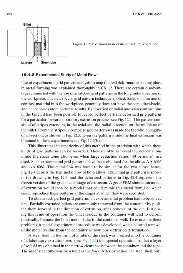
350 FEA of Extrusion
Figure 19.2. Extrusion in steel shell inside the container.
19.1.2 Experimental Study of Metal Flow
Use of experimental grid pattern analysis to map the real deformations taking placein metal forming was explained thoroughly in Ch. 12. There are certain disadvan-tages connected with the use of scratched grid patterns in the longitudinal section ofthe workpiece. The new special grid pattern technique applied, based on insertion ofcontrast material into the workpiece, generally does not have the same drawbacks,and hence yields more accurate results. By insertion of radial and axial contrast pinsin the billet, it has been possible to record perfect partially deformed grid patternsfor a particular forward laboratory extrusion process; see Fig. 12.4. The pattern con-sisted of stripes extending in the axial and the radial direction on the midplane ofthe billet. From the stripes, a complete grid pattern was made for the whole longitu-dinal section, as shown in Fig. 12.5. Even the pattern inside the final extrusion wasobtained in these experiments; see Fig. 12.6(b).
This illustrates the superiority of this method in the precision with which thesekinds of grid patterns can be recorded. They are able to reveal the deformationsinside the shear zone also, even when large reduction ratios (40 or more), areused. Such experimental grid patterns have been obtained for the alloys AA 6063and AA 6082. The metal flow was found to be similar for the two alloys; hence,Fig. 12.4 depicts the true metal flow of both alloys. The initial grid pattern is shownin the drawing in Fig. 12.3, and the deformed patterns in Fig. 12.4 represent thefrozen version of the grid at each stage of extrusion. A good FEM simulation modelof extrusion would then be a model that could mimic this metal flow, i.e., whichcould reproduce these patterns at the stages at which they were recorded.
To obtain such perfect grid patterns, an experimental problem had to be solvedfirst. Partially extruded billets are commonly removed from the container by push-ing them forward in the direction of extrusion, after removal of the die. But dur-ing this removal operation the billet residue in the container will tend to deformplastically, because the billet metal sticks to the container wall. To overcome theseproblems, a special experimental procedure was developed, which allowed removalof the metal residue from the container without post-extrusion deformation.
A steel shell, in the form of a tube of die steel, was inserted into the containerof a laboratory extrusion press (see Fig. 19.2) in a special operation, so that a layerof soft Al was obtained in the narrow clearance between the container and the tube.The inner steel tube was then used as the liner. After extrusion, the steel shell, with
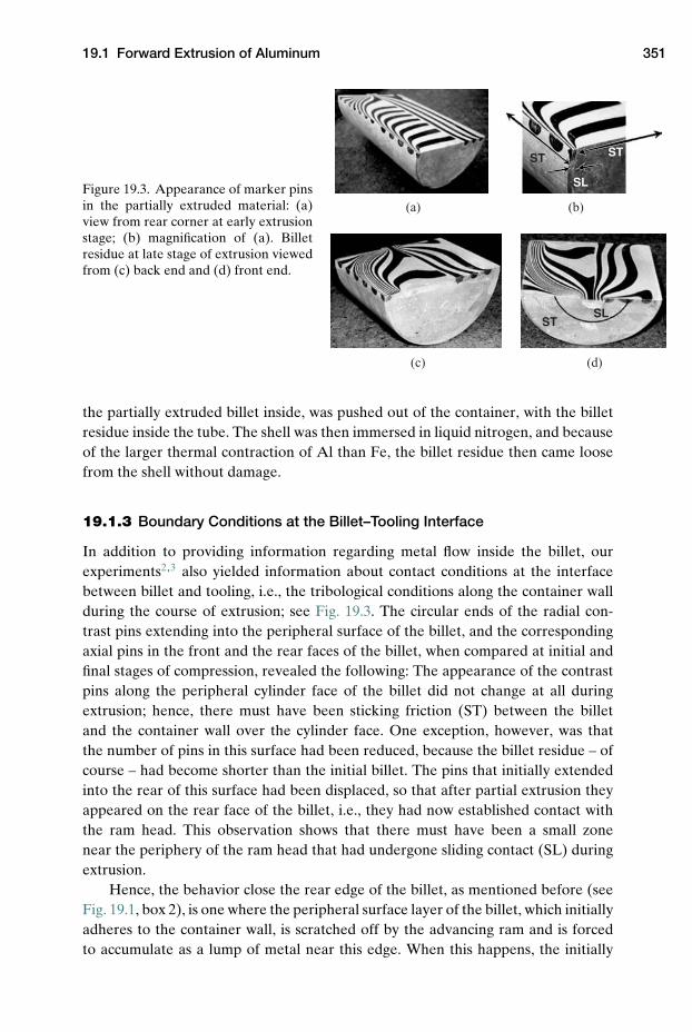
19.1 Forward Extrusion of Aluminum 351
ST ST
SL
STSL
(a) (b)
(d)(c)
Figure 19.3. Appearance of marker pinsin the partially extruded material: (a)view from rear corner at early extrusionstage; (b) magnification of (a). Billetresidue at late stage of extrusion viewedfrom (c) back end and (d) front end.
the partially extruded billet inside, was pushed out of the container, with the billetresidue inside the tube. The shell was then immersed in liquid nitrogen, and becauseof the larger thermal contraction of Al than Fe, the billet residue then came loosefrom the shell without damage.
19.1.3 Boundary Conditions at the Billet–Tooling Interface
In addition to providing information regarding metal flow inside the billet, ourexperiments2,3 also yielded information about contact conditions at the interfacebetween billet and tooling, i.e., the tribological conditions along the container wallduring the course of extrusion; see Fig. 19.3. The circular ends of the radial con-trast pins extending into the peripheral surface of the billet, and the correspondingaxial pins in the front and the rear faces of the billet, when compared at initial andfinal stages of compression, revealed the following: The appearance of the contrastpins along the peripheral cylinder face of the billet did not change at all duringextrusion; hence, there must have been sticking friction (ST) between the billetand the container wall over the cylinder face. One exception, however, was thatthe number of pins in this surface had been reduced, because the billet residue – ofcourse – had become shorter than the initial billet. The pins that initially extendedinto the rear of this surface had been displaced, so that after partial extrusion theyappeared on the rear face of the billet, i.e., they had now established contact withthe ram head. This observation shows that there must have been a small zonenear the periphery of the ram head that had undergone sliding contact (SL) duringextrusion.
Hence, the behavior close the rear edge of the billet, as mentioned before (seeFig. 19.1, box 2), is one where the peripheral surface layer of the billet, which initiallyadheres to the container wall, is scratched off by the advancing ram and is forcedto accumulate as a lump of metal near this edge. When this happens, the initially
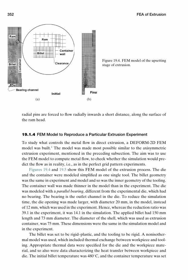
352 FEA of Extrusion
(a) (b)
Figure 19.4. FEM model of the upsettingstage of extrusion.
radial pins are forced to flow radially inwards a short distance, along the surface ofthe ram head.
19.1.4 FEM Model to Reproduce a Particular Extrusion Experiment
To study what controls the metal flow in direct extrusion, a DEFORM-2D FEMmodel was built.4 The model was made most possible similar to the axisymmetricextrusion experiment, mentioned in the preceding subsection. The aim was to usethe FEM model to compute metal flow, to check whether the simulation would pre-dict the flow as in reality, i.e., as in the perfect grid pattern experiments.
Figures 19.4 and 19.5 show this FEM model of the extrusion process. The dieand the container were modeled simplified as one single tool. The billet geometrywas the same in experiment and model and so was the inner geometry of the tooling.The container wall was made thinner in the model than in the experiment. The diewas modeled with a parallel bearing, different from the experimental die, which hadno bearing. The bearing is the outlet channel in the die. To reduce the simulationtime, the die opening was made larger, with diameter 20 mm, in the model, insteadof 12 mm, which was used in the experiment. Hence, whereas the reduction ratio was39.1 in the experiment, it was 14.1 in the simulation. The applied billet had 150 mmlength and 73 mm diameter. The diameter of the shell, which was used as extrusioncontainer, was 75 mm. These dimensions were the same in the simulation model andin the experiment.
The billet was set to be rigid–plastic, and the tooling to be rigid. A nonisother-mal model was used, which included thermal exchange between workpiece and tool-ing. Appropriate thermal data were specified for the die and the workpiece mate-rial, and so also were data characterizing the heat transfer between workpiece anddie. The initial billet temperature was 480◦C, and the container temperature was set
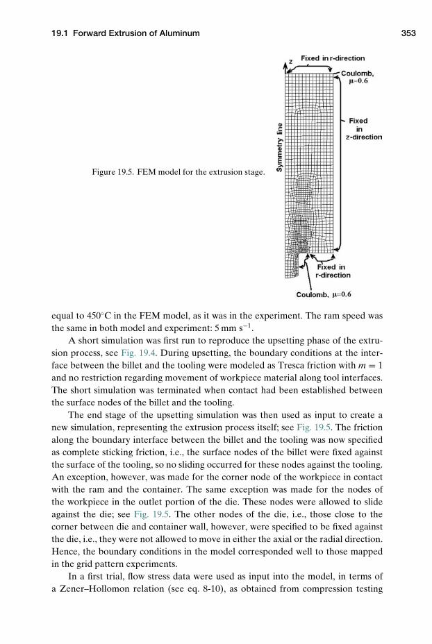
19.1 Forward Extrusion of Aluminum 353
Figure 19.5. FEM model for the extrusion stage.
equal to 450◦C in the FEM model, as it was in the experiment. The ram speed wasthe same in both model and experiment: 5 mm s−1.
A short simulation was first run to reproduce the upsetting phase of the extru-sion process, see Fig. 19.4. During upsetting, the boundary conditions at the inter-face between the billet and the tooling were modeled as Tresca friction with m = 1and no restriction regarding movement of workpiece material along tool interfaces.The short simulation was terminated when contact had been established betweenthe surface nodes of the billet and the tooling.
The end stage of the upsetting simulation was then used as input to create anew simulation, representing the extrusion process itself; see Fig. 19.5. The frictionalong the boundary interface between the billet and the tooling was now specifiedas complete sticking friction, i.e., the surface nodes of the billet were fixed againstthe surface of the tooling, so no sliding occurred for these nodes against the tooling.An exception, however, was made for the corner node of the workpiece in contactwith the ram and the container. The same exception was made for the nodes ofthe workpiece in the outlet portion of the die. These nodes were allowed to slideagainst the die; see Fig. 19.5. The other nodes of the die, i.e., those close to thecorner between die and container wall, however, were specified to be fixed againstthe die, i.e., they were not allowed to move in either the axial or the radial direction.Hence, the boundary conditions in the model corresponded well to those mappedin the grid pattern experiments.
In a first trial, flow stress data were used as input into the model, in terms ofa Zener–Hollomon relation (see eq. 8-10), as obtained from compression testing
354 FEA of Extrusion
of the alloy AA 6082 in a Gleeble test machine. The tests were run at differ-ent temperatures in the range 400–500◦C, for constant strain rates of 0.1, 1.0, and10 s−1 in each test, compressing small cylinders up to the total average strain of 1.The load–stroke curve was recorded in the tests, and true stress–strain curves werederived from them, correcting the data for the effect of friction in the compressiontest. The flow stress of the AA 6082 alloy was then described by a Zener–Hollomonfit on basis of this experimental data (see Example 8.5):
σ = 10.0102
sinh−1
(
ε exp( 152176.632
8.314T
)9.90 × 10¹²
) 17.643
(19-1)
After the model had been created, a number of simulations were run to study theeffect of various extrusion parameters on the metal flow, using these flow stressdata. The input parameters (friction, thermal conditions of billet and container,etc.) were varied within a realistic range, but all simulations yielded more or lessthe same flow. Hence, the metal flow seemed not to depend significantly on any ofthese traditional extrusion parameters. The simulation result also deviated from theexperiment, especially with regard to the appearance of the shear zone, which wasless localized in the simulations than in the experiment.
In a final trial, flow stress data on the workpiece material were changed, becausethe shear deformations in the shear zone did not localize as much in simulation asin the experiments. Simulation predicted an effective strain rate close to 1 s−1 inthis shear zone, so the flow stress was decreased for this particular strain rate, whilethe flow stress for other strain rates was kept unchanged. Now the metal flow wasaltered significantly, and became much more similar to the experimental flow. Goodcorrespondence was obtained this way when the flow stress was reduced by 20% inthe shear zone below the data from the compression test.
Metal flow very close to the experimental flow was then finally obtained, asshown in Fig. 19.6. This was for the same discard lengths as in the experiments;see Fig. 12.4. The conclusion is that there is good overall correspondence betweensimulated and experimental metal flow, with the exception of the first two stages ofextrusion, where there is less forward flow in the core of the billet in simulation thanin the experiment.
19.1.5 Simulation Results from the FEM Model of Forward Extrusion
The distribution of the effective strain rate (s−1) inside the billet at a particularstage of extrusion was now determined by the simulation model; see Fig. 12.4 andFig. 19.7. As this figure depicts, two zones of different deformation characteristicsbecome visible in the interior of the billet. These zones are not readily revealed bythe deformed grid pattern itself. In addition to the dead zones in the corner betweenthe die and the container and adjacent to the ram, there is also a tertiary dead zonein the core of the billet. Moreover, in between this dead zone and the secondarydead zone in the billet adjacent to the ram, there is an arrow-shaped secondary
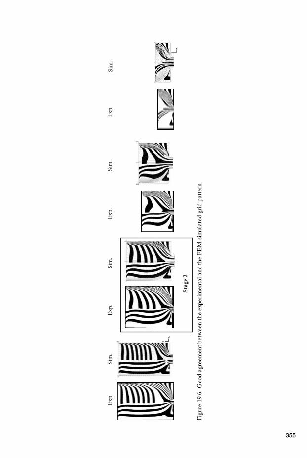
Exp
.E
xp.
Exp
.E
xp.
Sim
.S
im.
Sim
.S
im.
Stag
e 2
X
X
Y
Y
Fig
ure
19.6
.G
ood
agre
emen
tbet
wee
nth
eex
peri
men
tala
ndth
eF
EM
-sim
ulat
edgr
idpa
tter
n.
355
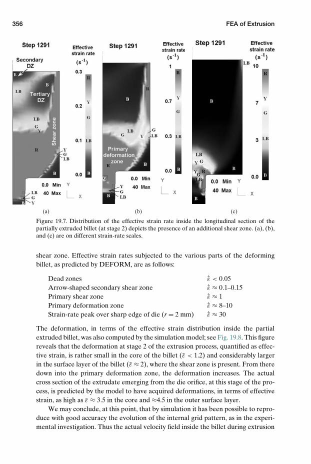
356 FEA of Extrusion
(a) (b) (c)
Figure 19.7. Distribution of the effective strain rate inside the longitudinal section of thepartially extruded billet (at stage 2) depicts the presence of an additional shear zone. (a), (b),and (c) are on different strain-rate scales.
shear zone. Effective strain rates subjected to the various parts of the deformingbillet, as predicted by DEFORM, are as follows:
Dead zones ˙ε < 0.05Arrow-shaped secondary shear zone ˙ε ≈ 0.1–0.15Primary shear zone ˙ε ≈ 1Primary deformation zone ˙ε ≈ 8–10Strain-rate peak over sharp edge of die (r = 2 mm) ˙ε ≈ 30
The deformation, in terms of the effective strain distribution inside the partialextruded billet, was also computed by the simulation model; see Fig. 19.8. This figurereveals that the deformation at stage 2 of the extrusion process, quantified as effec-tive strain, is rather small in the core of the billet (ε < 1.2) and considerably largerin the surface layer of the billet (ε ≈ 2), where the shear zone is present. From theredown into the primary deformation zone, the deformation increases. The actualcross section of the extrudate emerging from the die orifice, at this stage of the pro-cess, is predicted by the model to have acquired deformations, in terms of effectivestrain, as high as ε ≈ 3.5 in the core and ≈4.5 in the outer surface layer.
We may conclude, at this point, that by simulation it has been possible to repro-duce with good accuracy the evolution of the internal grid pattern, as in the experi-mental investigation. Thus the actual velocity field inside the billet during extrusion
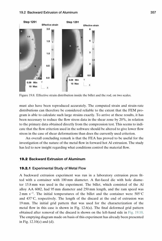
19.2 Backward Extrusion of Aluminum 357
Figure 19.8. Effective strain distribution inside the billet and the rod, on two scales.
must also have been reproduced accurately. The computed strain and strain-ratedistributions can therefore be considered reliable to the extent that the FEM pro-gram is able to calculate such large strains exactly. To arrive at these results, it hasbeen necessary to reduce the flow stress data in the shear zone by 20%, in relationto the primary data obtained directly from the compression test. This seems to indi-cate that the flow criterion used in the software should be altered to give lower flowstress in the case of shear deformations than does the currently used criterion.
An overall concluding remark is that the FEA has proved to be useful for theinvestigation of the nature of the metal flow in forward hot Al extrusion. The studyhas led to new insight regarding what conditions control the material flow.
19.2 Backward Extrusion of Aluminum
19.2.1 Experimental Study of Metal Flow
A backward extrusion experiment was run in a laboratory extrusion press fit-ted with a container with 100 mm diameter. A flat-faced die with hole diame-ter 15.8 mm was used in the experiment. The billet, which consisted of the Alalloy AA 6082, had 95 mm diameter and 250 mm length, and the ram speed was2 mm s−1. The initial temperatures of the billet and the container were 505◦Cand 437◦C, respectively. The length of the discard at the end of extrusion was19 mm. The initial grid pattern that was used for the characterization of themetal flow in this case is shown in Fig. 12.6(a). The final deformed grid patternobtained after removal of the discard is shown on the left-hand side in Fig. 19.10.The emptying diagram made on basis of this experiment has already been presentedin Fig. 12.10(c) and (d).
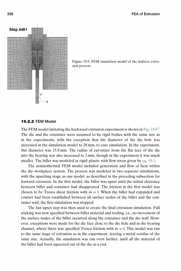
358 FEA of Extrusion
Figure 19.9. FEM simulation model of the indirect extru-sion process.
19.2.2 FEM Model
The FEM model imitating the backward extrusion experiment is shown in Fig. 19.9.5
The die and the container were assumed to be rigid bodies with the same size asin the experiments, with the exception that the diameter of the die hole wasincreased in the simulation model to 28 mm, to ease simulation. In the experiment,this diameter was 15.8 mm. The radius of curvature from the flat face of the dieinto the bearing was also increased to 2 mm, though in the experiment it was muchsmaller. The billet was modeled as rigid–plastic with flow stress given by eq. 19-1.
The nonisothermal FEM model included generation and flow of heat withinthe die–workpiece system. The process was modeled in two separate simulations,with the upsetting stage as one model, as described in the preceding subsection forforward extrusion. In the first model, the billet was upset until the initial clearancebetween billet and container had disappeared. The friction in the first model waschosen to be Tresca shear friction with m = l. When the billet had expanded andcontact had been established between all surface nodes of the billet and the con-tainer wall, the first simulation was stopped.
The last upset step was then used to create the final extrusion simulation. Fullsticking was now specified between billet material and tooling, i.e., no movement ofthe surface nodes of the billet occurred along the container and the die wall. How-ever, exceptions were made for the die face close to the die hole and in the bearingchannel, where there was specified Tresca friction with m = l. This model was runto the same stage of extrusion as in the experiment, leaving a metal residue of thesame size. Actually, the simulation was run even further, until all the material ofthe billet had been squeezed out of the die as a rod.
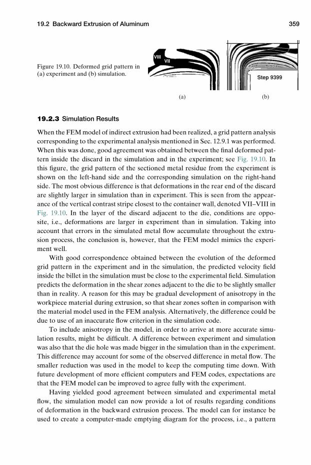
19.2 Backward Extrusion of Aluminum 359
Step 9399
VIIIVII
(a) (b)
Figure 19.10. Deformed grid pattern in(a) experiment and (b) simulation.
19.2.3 Simulation Results
When the FEM model of indirect extrusion had been realized, a grid pattern analysiscorresponding to the experimental analysis mentioned in Sec. 12.9.1 was performed.When this was done, good agreement was obtained between the final deformed pat-tern inside the discard in the simulation and in the experiment; see Fig. 19.10. Inthis figure, the grid pattern of the sectioned metal residue from the experiment isshown on the left-hand side and the corresponding simulation on the right-handside. The most obvious difference is that deformations in the rear end of the discardare slightly larger in simulation than in experiment. This is seen from the appear-ance of the vertical contrast stripe closest to the container wall, denoted VII–VIII inFig. 19.10. In the layer of the discard adjacent to the die, conditions are oppo-site, i.e., deformations are larger in experiment than in simulation. Taking intoaccount that errors in the simulated metal flow accumulate throughout the extru-sion process, the conclusion is, however, that the FEM model mimics the experi-ment well.
With good correspondence obtained between the evolution of the deformedgrid pattern in the experiment and in the simulation, the predicted velocity fieldinside the billet in the simulation must be close to the experimental field. Simulationpredicts the deformation in the shear zones adjacent to the die to be slightly smallerthan in reality. A reason for this may be gradual development of anisotropy in theworkpiece material during extrusion, so that shear zones soften in comparison withthe material model used in the FEM analysis. Alternatively, the difference could bedue to use of an inaccurate flow criterion in the simulation code.
To include anisotropy in the model, in order to arrive at more accurate simu-lation results, might be difficult. A difference between experiment and simulationwas also that the die hole was made bigger in the simulation than in the experiment.This difference may account for some of the observed difference in metal flow. Thesmaller reduction was used in the model to keep the computing time down. Withfuture development of more efficient computers and FEM codes, expectations arethat the FEM model can be improved to agree fully with the experiment.
Having yielded good agreement between simulated and experimental metalflow, the simulation model can now provide a lot of results regarding conditionsof deformation in the backward extrusion process. The model can for instance beused to create a computer-made emptying diagram for the process, i.e., a pattern
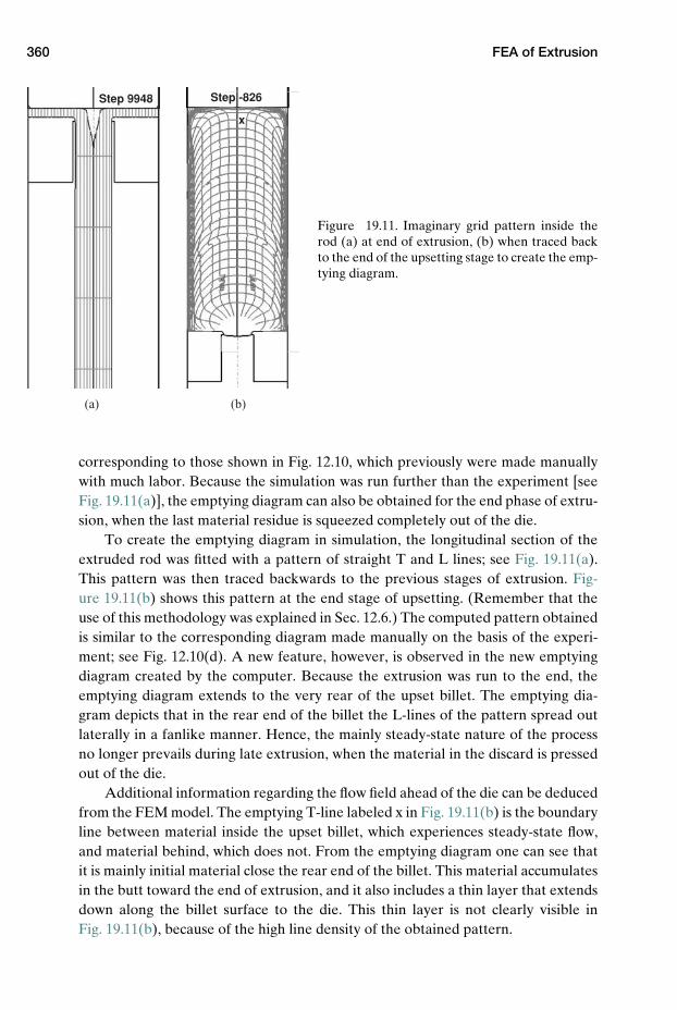
360 FEA of Extrusion
Step 9948 Step -826
x
(a) (b)
Figure 19.11. Imaginary grid pattern inside therod (a) at end of extrusion, (b) when traced backto the end of the upsetting stage to create the emp-tying diagram.
corresponding to those shown in Fig. 12.10, which previously were made manuallywith much labor. Because the simulation was run further than the experiment [seeFig. 19.11(a)], the emptying diagram can also be obtained for the end phase of extru-sion, when the last material residue is squeezed completely out of the die.
To create the emptying diagram in simulation, the longitudinal section of theextruded rod was fitted with a pattern of straight T and L lines; see Fig. 19.11(a).This pattern was then traced backwards to the previous stages of extrusion. Fig-ure 19.11(b) shows this pattern at the end stage of upsetting. (Remember that theuse of this methodology was explained in Sec. 12.6.) The computed pattern obtainedis similar to the corresponding diagram made manually on the basis of the experi-ment; see Fig. 12.10(d). A new feature, however, is observed in the new emptyingdiagram created by the computer. Because the extrusion was run to the end, theemptying diagram extends to the very rear of the upset billet. The emptying dia-gram depicts that in the rear end of the billet the L-lines of the pattern spread outlaterally in a fanlike manner. Hence, the mainly steady-state nature of the processno longer prevails during late extrusion, when the material in the discard is pressedout of the die.
Additional information regarding the flow field ahead of the die can be deducedfrom the FEM model. The emptying T-line labeled x in Fig. 19.11(b) is the boundaryline between material inside the upset billet, which experiences steady-state flow,and material behind, which does not. From the emptying diagram one can see thatit is mainly initial material close the rear end of the billet. This material accumulatesin the butt toward the end of extrusion, and it also includes a thin layer that extendsdown along the billet surface to the die. This thin layer is not clearly visible inFig. 19.11(b), because of the high line density of the obtained pattern.
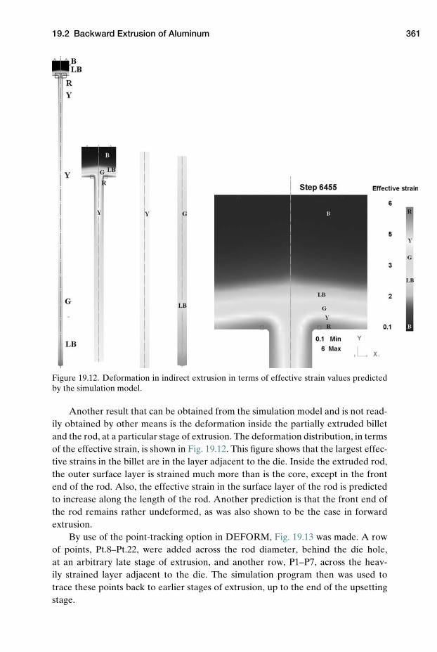
19.2 Backward Extrusion of Aluminum 361
Figure 19.12. Deformation in indirect extrusion in terms of effective strain values predictedby the simulation model.
Another result that can be obtained from the simulation model and is not read-ily obtained by other means is the deformation inside the partially extruded billetand the rod, at a particular stage of extrusion. The deformation distribution, in termsof the effective strain, is shown in Fig. 19.12. This figure shows that the largest effec-tive strains in the billet are in the layer adjacent to the die. Inside the extruded rod,the outer surface layer is strained much more than is the core, except in the frontend of the rod. Also, the effective strain in the surface layer of the rod is predictedto increase along the length of the rod. Another prediction is that the front end ofthe rod remains rather undeformed, as was also shown to be the case in forwardextrusion.
By use of the point-tracking option in DEFORM, Fig. 19.13 was made. A rowof points, Pt.8–Pt.22, were added across the rod diameter, behind the die hole,at an arbitrary late stage of extrusion, and another row, P1–P7, across the heav-ily strained layer adjacent to the die. The simulation program then was used totrace these points back to earlier stages of extrusion, up to the end of the upsettingstage.
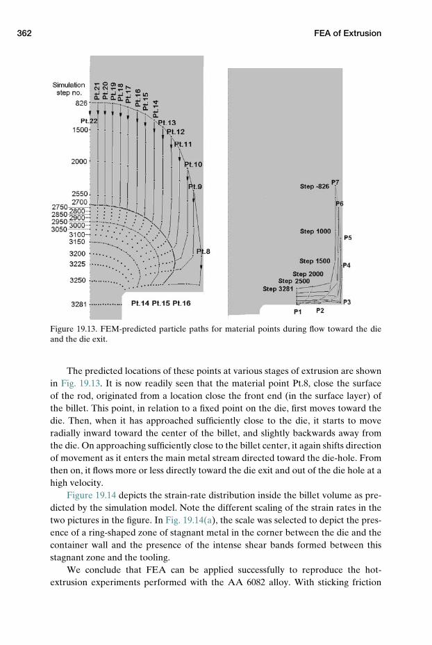
362 FEA of Extrusion
Figure 19.13. FEM-predicted particle paths for material points during flow toward the dieand the die exit.
The predicted locations of these points at various stages of extrusion are shownin Fig. 19.13. It is now readily seen that the material point Pt.8, close the surfaceof the rod, originated from a location close the front end (in the surface layer) ofthe billet. This point, in relation to a fixed point on the die, first moves toward thedie. Then, when it has approached sufficiently close to the die, it starts to moveradially inward toward the center of the billet, and slightly backwards away fromthe die. On approaching sufficiently close to the billet center, it again shifts directionof movement as it enters the main metal stream directed toward the die-hole. Fromthen on, it flows more or less directly toward the die exit and out of the die hole at ahigh velocity.
Figure 19.14 depicts the strain-rate distribution inside the billet volume as pre-dicted by the simulation model. Note the different scaling of the strain rates in thetwo pictures in the figure. In Fig. 19.14(a), the scale was selected to depict the pres-ence of a ring-shaped zone of stagnant metal in the corner between the die and thecontainer wall and the presence of the intense shear bands formed between thisstagnant zone and the tooling.
We conclude that FEA can be applied successfully to reproduce the hot-extrusion experiments performed with the AA 6082 alloy. With sticking friction
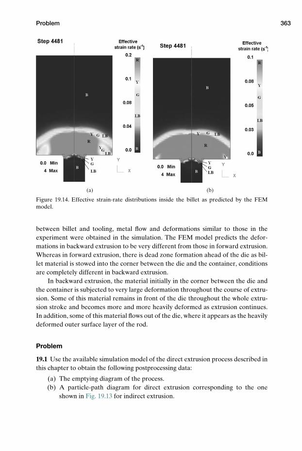
Problem 363
(a) (b)
Figure 19.14. Effective strain-rate distributions inside the billet as predicted by the FEMmodel.
between billet and tooling, metal flow and deformations similar to those in theexperiment were obtained in the simulation. The FEM model predicts the defor-mations in backward extrusion to be very different from those in forward extrusion.Whereas in forward extrusion, there is dead zone formation ahead of the die as bil-let material is stowed into the corner between the die and the container, conditionsare completely different in backward extrusion.
In backward extrusion, the material initially in the corner between the die andthe container is subjected to very large deformation throughout the course of extru-sion. Some of this material remains in front of the die throughout the whole extru-sion stroke and becomes more and more heavily deformed as extrusion continues.In addition, some of this material flows out of the die, where it appears as the heavilydeformed outer surface layer of the rod.
Problem
19.1 Use the available simulation model of the direct extrusion process described inthis chapter to obtain the following postprocessing data:
(a) The emptying diagram of the process.(b) A particle-path diagram for direct extrusion corresponding to the one
shown in Fig. 19.13 for indirect extrusion.

364 FEA of Extrusion
NOTES
1. Valberg, H., and Sandbakk, Ø.: “Direct non-lubricated Al-extrusion partitioned intothe sub-processes shearing, scratching, radial compression and extrusion,” Proc. 6th Int.Conf. on Material Forming, Salerno, Italy, 2003, pp. 307–310.
2. Valberg, H., and Uyyuru, R. K.: “New accurate experimental techniques to quan-tify metal flow inside workpiece – and along boundary interface of workpiece – inmetal forming,” Proc. 2nd Int. Conf. on Tribology in Manufacturing Processes, Nyborg,Denmark, 2004, Vol. 2, pp. 453–474.
3. Valberg, H.: “Experimental techniques to characterize large plastic deformations inunlubricated hot aluminium extrusion,” Key Engineering Materials, Vol. 367, 2008,pp. 17–24.
4. Valberg, H., and Pohl, C.: “Boundary conditions and metal flow in forward extrusion ofaluminium alloys,” Conf. Proc. Euromech 435, Valencienne, 2002, pp. 33–45.
5. Valberg, H., and Misiolek, W. Z.: “Plastic deformations in indirect hot extrusion of analuminium alloy characterised by FEM-analysis with experiment,” Proc. 9th EsaformConf., Glasgow, 2006, pp. 487–490.
REFERENCE
Valberg, H.: “Experimental techniques to characterize large plastic deformations in unlubri-cated hot aluminium extrusion,” Key Engineering Materials, Vol. 367, 2008, pp. 17–24.
20 Rolling
Rolling is the metal forming process by which the largest amount of metal is beingworked in the world. In terms of tonnage of metal, this process must therefore beconsidered the most important one. In Sec. 2.2.4, some important aspects of thisforming process were discussed. In this chapter, some additional practical topicsimportant in industrial rolling will be considered. The treatment will be limited toflat rolling; section rolling is outside the scope of this book.
The velocity conditions of the workpiece along the roll surface, through theroll gap, will first be considered. It will be shown that the velocity conditions heredepend on whether there is sliding friction or sticking friction between the rolls andthe workpiece. In industrial rolling, it is important to be able to estimate the loadsacting on the rolls from the workpiece, i.e., to determine the required rolling force.Because of this, a large number of rolling force formulas have been developed overthe time. One such simple formula will be considered in this chapter. Afterwards, itwill be shown how the strain and strain-rate conditions vary throughout the roll gap,if one assumes homogeneous deformation in the workpiece material during rolling.In that case, a rectangular slab element of material that enters the roll gap shouldmaintain its rectangular shape during passage through the gap. Finally, it will beshown how an approximate estimation of the contact pressure over the roll surfacecan be deduced by means of the slab method. This expression is valid when there ishomogeneous deformation in the roll pass.
20.1 Velocities in the Roll Gap in Flat Rolling
The contact conditions along the boundary interface between the roll and the work-piece material can, in principle, be characterized either by sticking friction or bysliding friction. The velocity conditions for the material particles on the surface ofthe workpiece inside the roll gap will be significantly different in the two cases offriction.
Consider a material particle on the workpiece surface, which moves in the direc-tion toward the roll gap with the velocity v0. If there is sticking friction between theroll and the workpiece material, this particle will immediately, when it establishes
365
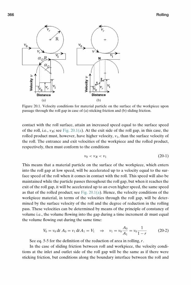
366 Rolling
(a) (b)
Figure 20.1. Velocity conditions for material particle on the surface of the workpiece uponpassage through the roll gap in case of (a) sticking friction and (b) sliding friction.
contact with the roll surface, attain an increased speed equal to the surface speedof the roll, i.e., vR; see Fig. 20.1(a). At the exit side of the roll gap, in this case, therolled product must, however, have higher velocity, v1, than the surface velocity ofthe roll. The entrance and exit velocities of the workpiece and the rolled product,respectively, then must conform to the conditions
v0 < vR < v1 (20-1)
This means that a material particle on the surface of the workpiece, which entersinto the roll gap at low speed, will be accelerated up to a velocity equal to the sur-face speed of the roll when it comes in contact with the roll. This speed will also bemaintained while the particle passes throughout the roll gap, but when it reaches theexit of the roll gap, it will be accelerated up to an even higher speed, the same speedas that of the rolled product; see Fig. 20.1(a). Hence, the velocity conditions of theworkpiece material, in terms of the velocities through the roll gap, will be deter-mined by the surface velocity of the roll and the degree of reduction in the rollingpass. These velocities can be determined by means of the principle of constancy ofvolume i.e., the volume flowing into the gap during a time increment dt must equalthe volume flowing out during the same time:
V0 = v0 dt A0 = v1 dt A1 = V1 ⇒ v1 = v0A0
A1= v0
11 − r
(20-2)
See eq. 5-5 for the definition of the reduction of area in rolling, r .In the case of sliding friction between roll and workpiece, the velocity condi-
tions at the inlet and outlet side of the roll gap will be the same as if there weresticking friction, but conditions along the boundary interface between the roll and
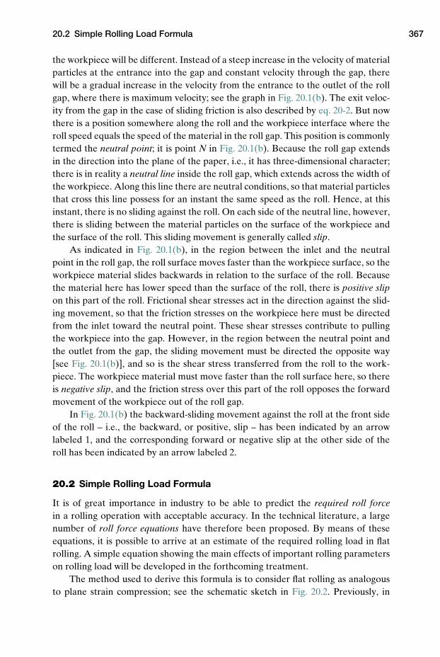
20.2 Simple Rolling Load Formula 367
the workpiece will be different. Instead of a steep increase in the velocity of materialparticles at the entrance into the gap and constant velocity through the gap, therewill be a gradual increase in the velocity from the entrance to the outlet of the rollgap, where there is maximum velocity; see the graph in Fig. 20.1(b). The exit veloc-ity from the gap in the case of sliding friction is also described by eq. 20-2. But nowthere is a position somewhere along the roll and the workpiece interface where theroll speed equals the speed of the material in the roll gap. This position is commonlytermed the neutral point; it is point N in Fig. 20.1(b). Because the roll gap extendsin the direction into the plane of the paper, i.e., it has three-dimensional character;there is in reality a neutral line inside the roll gap, which extends across the width ofthe workpiece. Along this line there are neutral conditions, so that material particlesthat cross this line possess for an instant the same speed as the roll. Hence, at thisinstant, there is no sliding against the roll. On each side of the neutral line, however,there is sliding between the material particles on the surface of the workpiece andthe surface of the roll. This sliding movement is generally called slip.
As indicated in Fig. 20.1(b), in the region between the inlet and the neutralpoint in the roll gap, the roll surface moves faster than the workpiece surface, so theworkpiece material slides backwards in relation to the surface of the roll. Becausethe material here has lower speed than the surface of the roll, there is positive slipon this part of the roll. Frictional shear stresses act in the direction against the slid-ing movement, so that the friction stresses on the workpiece here must be directedfrom the inlet toward the neutral point. These shear stresses contribute to pullingthe workpiece into the gap. However, in the region between the neutral point andthe outlet from the gap, the sliding movement must be directed the opposite way[see Fig. 20.1(b)], and so is the shear stress transferred from the roll to the work-piece. The workpiece material must move faster than the roll surface here, so thereis negative slip, and the friction stress over this part of the roll opposes the forwardmovement of the workpiece out of the roll gap.
In Fig. 20.1(b) the backward-sliding movement against the roll at the front sideof the roll – i.e., the backward, or positive, slip – has been indicated by an arrowlabeled 1, and the corresponding forward or negative slip at the other side of theroll has been indicated by an arrow labeled 2.
20.2 Simple Rolling Load Formula
It is of great importance in industry to be able to predict the required roll forcein a rolling operation with acceptable accuracy. In the technical literature, a largenumber of roll force equations have therefore been proposed. By means of theseequations, it is possible to arrive at an estimate of the required rolling load in flatrolling. A simple equation showing the main effects of important rolling parameterson rolling load will be developed in the forthcoming treatment.
The method used to derive this formula is to consider flat rolling as analogousto plane strain compression; see the schematic sketch in Fig. 20.2. Previously, in
368 Rolling
Figure 20.2. Rolling considered as equivalent to plane straincompression to deduce a rolling load formula.
Sec. 13.2.1.1, the following expression was deduced for the compression force inplane strain compression of a specimen with height h and half width l:
F = 2σ√3
(1 + ml
4h
)l
The formula was developed assuming Tresca friction characterized by a frictionfactor m, and for a workpiece material of constant flow stress σ . The formula calcu-lates the required compression force for a specimen of one unit breadth, extendinginto the plane of the paper. For a specimen of breadth B, the corresponding force is
F = 2σ√3
(1 + ml
4h
)l B (20-3)
In Fig. 20.2, a rolling process is sketched, and a corresponding equivalent compres-sion process is added on top of the sketch, with hatched compression dies. As thefigure illustrates, the slab must be compressed down to a thickness equal to half ofthe final thickness in the rolling process, i.e., to a thickness equal to
h = 12
(h0 + h1) (20-4)
One-half of the workpiece inside the roll gap will then be compressed too much,while the other half is compressed too little. Thus one can assume rolling to beequivalent to plane strain compression down to half the thickness reduction used inthe rolling process.
Based upon this analogy, the rolling load in flat rolling, under plane strain con-ditions, can be expressed by the following formula:
F = 2σ√3
(1 + ml
2 (h0 + h1)
)l B (20-5)
In the literature it is sometimes recommended that the projected length of the arcof roll contact in this formula, i.e., l, should be replaced by the real length of thisarc, i.e., αDR; see Fig. 20.2. This increases the calculated rolling load somewhat, as
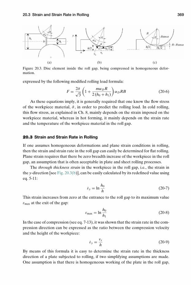
20.3 Strain and Strain Rate in Rolling 369
(a) (b) (c)
Figure 20.3. Disc element inside the roll gap, being compressed in homogeneous defor-mation.
expressed by the following modified rolling load formula:
F = 2σ√3
(1 + mαDR
2 (h0 + h1)
)αDRB (20-6)
As these equations imply, it is generally required that one know the flow stressof the workpiece material, σ , in order to predict the rolling load. In cold rolling,this flow stress, as explained in Ch. 8, mainly depends on the strain imposed on theworkpiece material, whereas in hot forming, it mainly depends on the strain rateand the temperature of the workpiece material in the roll gap.
20.3 Strain and Strain Rate in Rolling
If one assumes homogeneous deformations and plane strain conditions in rolling,then the strain and strain rate in the roll gap can easily be determined for flat rolling.Plane strain requires that there be zero breadth increase of the workpiece in the rollgap, an assumption that is often acceptable in plate and sheet rolling processes.
The through thickness strain in the workpiece in the roll gap, i.e., the strain inthe y-direction [see Fig. 20.3(b)], can be easily calculated by its redefined value usingeq. 5-11:
εy = lnh0
h(20-7)
This strain increases from zero at the entrance to the roll gap to its maximum valueεmax at the exit of the gap:
εmax = lnh0
h1(20-8)
In the case of compression (see eq. 7-13), it was shown that the strain rate in the com-pression direction can be expressed as the ratio between the compression velocityand the height of the workpiece:
εy = vs
h(20-9)
By means of this formula it is easy to determine the strain rate in the thicknessdirection of a plate subjected to rolling, if two simplifying assumptions are made.One assumption is that there is homogeneous working of the plate in the roll gap,
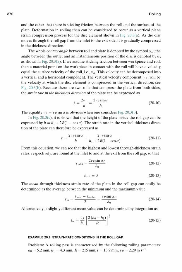
370 Rolling
and the other that there is sticking friction between the roll and the surface of theplate. Deformation in rolling then can be considered to occur as a vertical planestrain compression process for the disc element shown in Fig. 20.3(a). As the discmoves through the roll gap from the inlet to the exit side, it is gradually compressedin the thickness direction.
The whole contact angle between roll and plate is denoted by the symbol αD; theangle between the outlet and an instantaneous position of the disc is denoted by α,as shown in Fig. 20.3(a). If we assume sticking friction between workpiece and roll,then a material point on the workpiece in contact with the roll will have a velocityequal the surface velocity of the roll, i.e., vR. This velocity can be decomposed intoa vertical and a horizontal component. The vertical velocity component, v⊥, will bethe velocity at which the disc element is compressed in the vertical direction; seeFig. 20.3(b). Because there are two rolls that compress the plate from both sides,the strain rate in the thickness direction of the plate can be expressed as
ε = 2v⊥h
= 2vR sin α
h(20-10)
The equality v⊥ = vR sin α is obvious when one considers Fig. 20.3(b).In Fig. 20.3(c), it is shown that the height of the plate inside the roll gap can be
expressed by h = h1 + 2R(1 − cos α). The strain rate in the vertical thickness direc-tion of the plate can therefore be expressed as
ε = 2vR sin α
h= 2vR sin α
h1 + 2R(1 − cos α)(20-11)
From this equation, we can see that the highest and lowest through-thickness strainrates, respectively, are found at the inlet to and at the exit from the roll gap, so that
εinlet = 2vR sin αD
h0(20-12)
εexit = 0 (20-13)
The mean through-thickness strain rate of the plate in the roll gap can easily bedetermined as the average between the minimum and the maximum value,
εm = εinlet − εoutlet
2= vR sin αD
h0(20-14)
Alternatively, a slightly different mean value can be determined by integration as
εm = vR
h0
[2 (h0 − h1)
R
] 12
(20-15)
EXAMPLE 20.1: STRAIN-RATE CONDITIONS IN THE ROLL GAP
Problem: A rolling pass is characterized by the following rolling parameters:h0 = 5.2 mm, h1 = 4.3 mm, R = 215 mm, l = 13.9 mm, vR = 2.29 m s−1
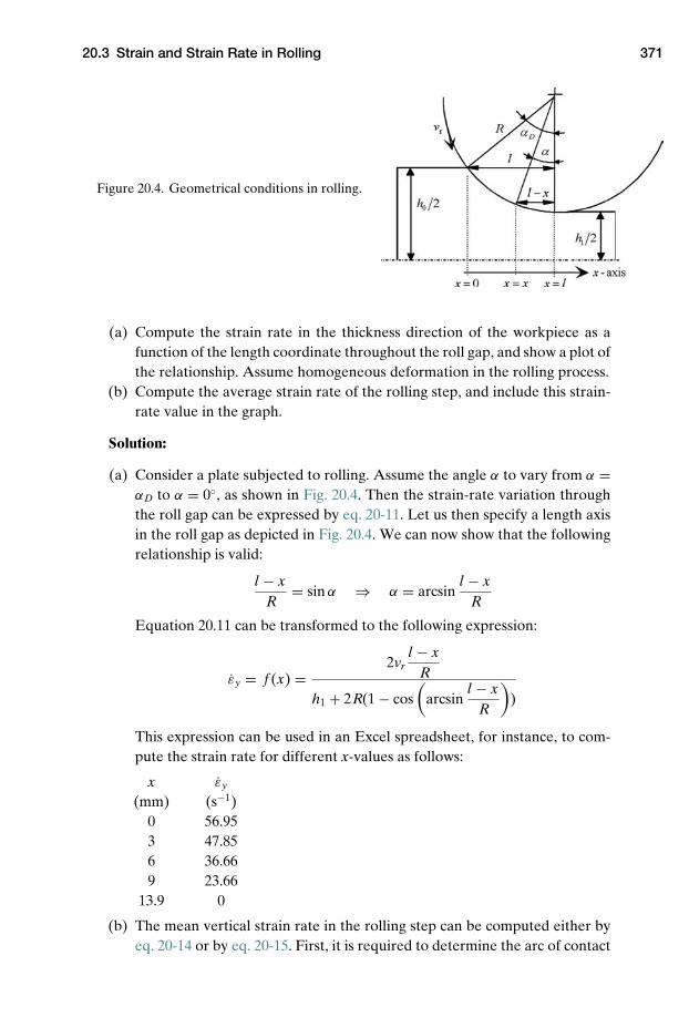
20.3 Strain and Strain Rate in Rolling 371
Figure 20.4. Geometrical conditions in rolling.
(a) Compute the strain rate in the thickness direction of the workpiece as afunction of the length coordinate throughout the roll gap, and show a plot ofthe relationship. Assume homogeneous deformation in the rolling process.
(b) Compute the average strain rate of the rolling step, and include this strain-rate value in the graph.
Solution:
(a) Consider a plate subjected to rolling. Assume the angle α to vary from α =αD to α = 0◦, as shown in Fig. 20.4. Then the strain-rate variation throughthe roll gap can be expressed by eq. 20-11. Let us then specify a length axisin the roll gap as depicted in Fig. 20.4. We can now show that the followingrelationship is valid:
l − xR
= sin α ⇒ α = arcsinl − x
R
Equation 20.11 can be transformed to the following expression:
εy = f (x) =2vr
l − xR
h1 + 2R(1 − cos(
arcsinl − x
R
))
This expression can be used in an Excel spreadsheet, for instance, to com-pute the strain rate for different x-values as follows:
x εy
(mm) (s−1)0 56.953 47.856 36.669 23.66
13.9 0
(b) The mean vertical strain rate in the rolling step can be computed either byeq. 20-14 or by eq. 20-15. First, it is required to determine the arc of contact
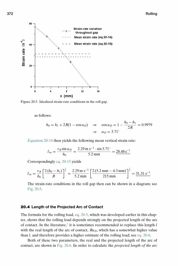
372 Rolling
Figure 20.5. Idealized strain-rate conditions in the roll gap.
as follows:
h0 = h1 + 2R(1 − cos αD) ⇒ cos αD = 1 − h0 − h1
2R= 0.9979
⇒ αD = 3.71◦
Equation 20-14 then yields the following mean vertical strain rate:
˙εm = vR sin αD
h0= 2.29 m s−1 · sin 3.71◦
5.2 mm= 28.48 s−1
Correspondingly eq. 20-15 yields
˙εm = vR
h0
[2 (h0 − h1)
R
] 12
= 2.29 m s−1
5.2 mm
[2 (5.2 mm − 4.3 mm)
215 mm
] 12
= 31.31 s−1
The strain-rate conditions in the roll gap then can be shown in a diagram; seeFig. 20.5.
20.4 Length of the Projected Arc of Contact
The formula for the rolling load, eq. 20-5, which was developed earlier in this chap-ter, shows that the rolling load depends strongly on the projected length of the arcof contact. In the literature,1 it is sometimes recommended to replace this length lwith the real length of the arc of contact, RαD, which has a somewhat higher valuethan l, and therefore provides a higher estimate of the rolling load; see eq. 20-6.
Both of these two parameters, the real and the projected length of the arc ofcontact, are shown in Fig. 20.6. In order to calculate the projected length of the arc

20.5 Pressure Distribution over the Arc of Contact of the Roll 373
Figure 20.6. Geometrical relationship in rolling.
of contact, the following approximate formula can be used (see Example 20.2):
l ≈√
R(h0 − h1) = √R�h (20-16)
This relationship is based on the assumption that the roll radius in the actual case ismuch bigger than the height reduction in the rolling pass.
EXAMPLE 20.2: FORMULA FOR THE PROJECTED LENGTH OF THE ARC OF CONTACT
Problem: Show that the length of the projected arc of contact in a rolling passapproximately equals the square root of the product of the roll radius and thethickness reduction in the rolling step.
Solution: The Pythagorean theorem, used on the hatched triangle in Fig. 20.6,yields the following expression:
R2 = l2 +(
R − �h2
)2
R2 = l2 + R2 − �hR + �h2
4
In rolling, most commonly �h � R, and the term �h2/4 can therefore beneglected. This yields
l2 = �hR ⇒ l ≈√
R(h0 − h1) = √R�h
20.5 Pressure Distribution over the Arc of Contact of the Roll
Attempts have been made to obtain expressions that accurately predict the contactpressure variation over the arc of contact of the roll. A theoretical analysis,2 basedon the slab method (see Fig. 20.7), provides the following pressure distribution:
For the entry zone, i.e., for 0 ≤ x ≤ xn :
σx,1 = 2σa
h
(xnxR
− x2
2R− µx
)+ C1
h(20-17)
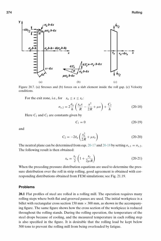
374 Rolling
(a) (b) (c)
Figure 20.7. (a) Stresses and (b) forces on a slab element inside the roll gap. (c) Velocityconditions.
For the exit zone, i.e., for xn ≤ x ≤ xe:
σx,2 = 2σa
h
(xnxR
− x2
2R+ µx
)+ C2
h(20-18)
Here C1 and C2 are constants given by
C1 = 0 (20-19)
and
C2 = −2σa
(x2
n
2R+ µxe
)(20-20)
The neutral plane can be determined from eqs. 20-17 and 20-18 by setting σx,1 = σx,2.The following result is then obtained:
xn = xe
2
(1 + xe
2µR
)(20-21)
When the preceding pressure distribution equations are used to determine the pres-sure distribution over the roll in strip rolling, good agreement is obtained with cor-responding distributions obtained from FEM simulations; see Fig. 21.19.
Problems
20.1 Flat profiles of steel are rolled in a rolling mill. The operation requires manyrolling steps where both flat and grooved passes are used. The initial workpiece is abillet with rectangular cross section 150 mm × 300 mm, as shown in the accompany-ing figure. The same figure shows how the cross section of the workpiece is reducedthroughout the rolling stands. During the rolling operation, the temperature of thesteel drops because of cooling, and the measured temperature in each rolling stepis also specified in the figure. It is desirable that the rolling load be kept below500 tons to prevent the rolling mill from being overloaded by fatigue.
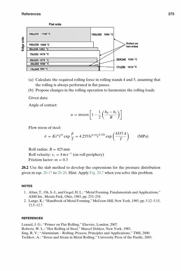
References 375
(a) Calculate the required rolling force in rolling stands 4 and 5, assuming thatthe rolling is always performed in flat passes.
(b) Propose changes in the rolling operation to harmonize the rolling loads.
Given data:
Angle of contact:
α = arccos[
1 − 12
(h0 − h1
R
)]
Flow stress of steel:
σ = Kεn ˙εm expβ
T= 4.2553ε0.19 ˙ε0.128 exp
(4337.4
T
)(MPa)
Roll radius: R = 425 mmRoll velocity: vr = 4 m s−1 (on roll periphery)Friction factor: m = 0.3
20.2 Use the slab method to develop the expressions for the pressure distributiongiven in eqs. 20-17 to 20-20. Hint: Apply Fig. 20.7 when you solve this problem.
NOTES
1. Altan, T., Oh, S.-I., and Gegel, H. L.: “Metal Forming, Fundamentals and Applications,”ASM Int., Metals Park, Ohio, 1983, pp. 253–254.
2. Lange, K.: “Handbook of Metal Forming,” McGraw-Hill, New York, 1985, pp. 5.12–5.15,12.5–12.7.
REFERENCES
Lenard, J. G.: “Primer on Flat Rolling,” Elsevier, London, 2007.Roberts, W. L.: “Hot Rolling of Steel,” Marcel Dekker, New York, 1983.Sing, R. V.: “Aluminium – Rolling; Process, Principles and Applications,” TMS, 2000.Tselikov, A.: “Stress and Strain in Metal Rolling,” University Press of the Pacific, 2003.
21 FEA of Rolling
Three different cases of metal rolling will be analyzed in this chapter by use of FEA.The simulation results obtained in each case will be examined in order to describethe mechanics of these typical industrial rolling situations. It will be shown that thedeformation process is indeed very different in slab rolling from what it is in striprolling because of the use of very different thickness-to-width ratios of material inthe roll gap. In addition, the effect of the use of a light pass in the slab rolling processis considered. The main rolling parameters used in the three different cases of rollinganalyzed here are specified in Table 21.1. The obtained results reveal clearly thatthe mechanics of rolling are complex. The deformation distribution obtained in theroll gap is found to depend strongly on the parameter � (see eq. 5-13), as well ason the reduction taken in the rolling step. Note that, in this chapter, slab rolling isconsidered as a hot rolling process applied to the alloy AA 3003. Strip rolling, onthe other hand, is considered as cold rolling process for an alloy with a flow stressdescribed by σ = 180ε0.1. In all cases considered here, plane strain FEM models areused to model the rolling process.
21.1 Hot Rolling of an Aluminum Slab in a Light Pass
To analyze the mechanics of deformation when utilizing a very light rolling pass, theupper half of the FEM model shown in Fig. 21.1 was made. To secure seizure of theslab upon entrance into the roll gap, a manipulator in the form of a small movingdie was placed at the rear end of the slab. In the beginning of the rolling process, themanipulator was moved with low velocity toward the rolls, in order to push the slabinto the roll gap.
The rotational velocity of the roll was specified sufficiently high, in relation tothe velocity of the die, that when the slab had been pushed sufficient deep into theroll gap, conditions of unaided entrance were achieved. The roll now started to pullthe slab in the direction of rolling, faster than the movement of the manipulator.
Figure 21.1(a) shows the tool and workpiece configuration at the start of thesimulation model. Now the rolls are positioned at one end of the slab and the push-ing die at the other end. At this instant, movement into the roll gap of the slab
376
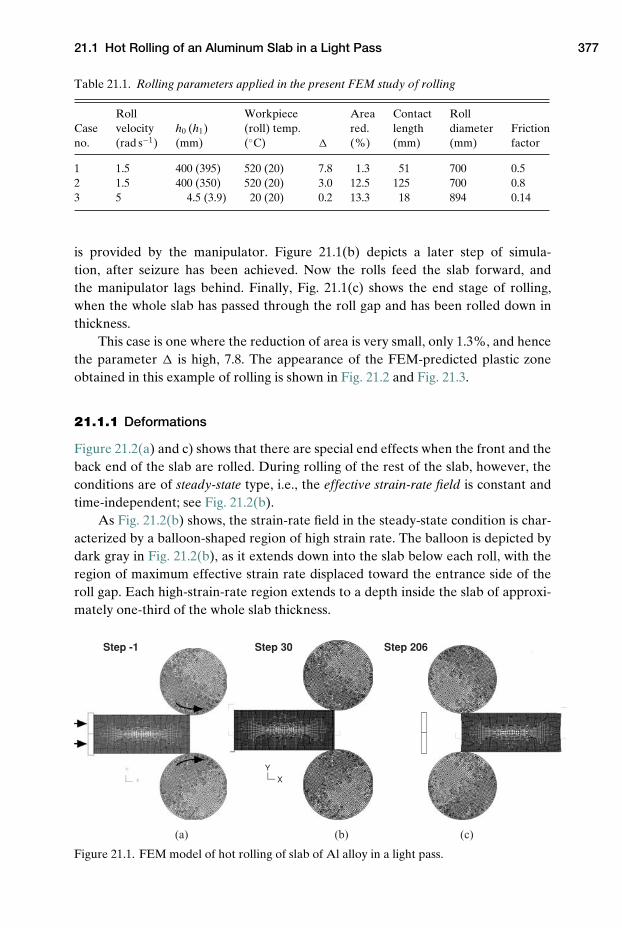
21.1 Hot Rolling of an Aluminum Slab in a Light Pass 377
Table 21.1. Rolling parameters applied in the present FEM study of rolling
Roll Workpiece Area Contact RollCase velocity h0 (h1) (roll) temp. red. length diameter Frictionno. (rad s−1) (mm) (◦C) � (%) (mm) (mm) factor
1 1.5 400 (395) 520 (20) 7.8 1.3 51 700 0.52 1.5 400 (350) 520 (20) 3.0 12.5 125 700 0.83 5 4.5 (3.9) 20 (20) 0.2 13.3 18 894 0.14
is provided by the manipulator. Figure 21.1(b) depicts a later step of simula-tion, after seizure has been achieved. Now the rolls feed the slab forward, andthe manipulator lags behind. Finally, Fig. 21.1(c) shows the end stage of rolling,when the whole slab has passed through the roll gap and has been rolled down inthickness.
This case is one where the reduction of area is very small, only 1.3%, and hencethe parameter � is high, 7.8. The appearance of the FEM-predicted plastic zoneobtained in this example of rolling is shown in Fig. 21.2 and Fig. 21.3.
21.1.1 Deformations
Figure 21.2(a) and c) shows that there are special end effects when the front and theback end of the slab are rolled. During rolling of the rest of the slab, however, theconditions are of steady-state type, i.e., the effective strain-rate field is constant andtime-independent; see Fig. 21.2(b).
As Fig. 21.2(b) shows, the strain-rate field in the steady-state condition is char-acterized by a balloon-shaped region of high strain rate. The balloon is depicted bydark gray in Fig. 21.2(b), as it extends down into the slab below each roll, with theregion of maximum effective strain rate displaced toward the entrance side of theroll gap. Each high-strain-rate region extends to a depth inside the slab of approxi-mately one-third of the whole slab thickness.
(a) (b) (c)
Step 30 Step 206
X
Y
Step -1
Figure 21.1. FEM model of hot rolling of slab of Al alloy in a light pass.
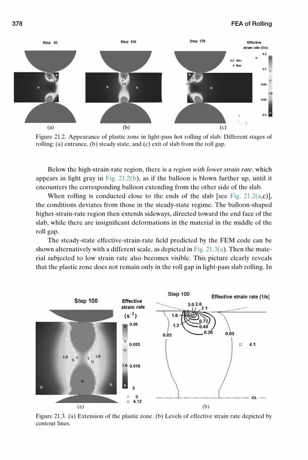
378 FEA of Rolling
Figure 21.2. Appearance of plastic zone in light-pass hot rolling of slab. Different stages ofrolling: (a) entrance, (b) steady state, and (c) exit of slab from the roll gap.
Below the high-strain-rate region, there is a region with lower strain rate, whichappears in light gray in Fig. 21.2(b), as if the balloon is blown further up, until itencounters the corresponding balloon extending from the other side of the slab.
When rolling is conducted close to the ends of the slab [see Fig. 21.2(a,c)],the conditions deviates from those in the steady-state regime. The balloon-shapedhigher-strain-rate region then extends sideways, directed toward the end face of theslab, while there are insignificant deformations in the material in the middle of theroll gap.
The steady-state effective-strain-rate field predicted by the FEM code can beshown alternatively with a different scale, as depicted in Fig. 21.3(a). Then the mate-rial subjected to low strain rate also becomes visible. This picture clearly revealsthat the plastic zone does not remain only in the roll gap in light-pass slab rolling. In
Step 100
(a) (b)
Figure 21.3. (a) Extension of the plastic zone. (b) Levels of effective strain rate depicted bycontour lines.
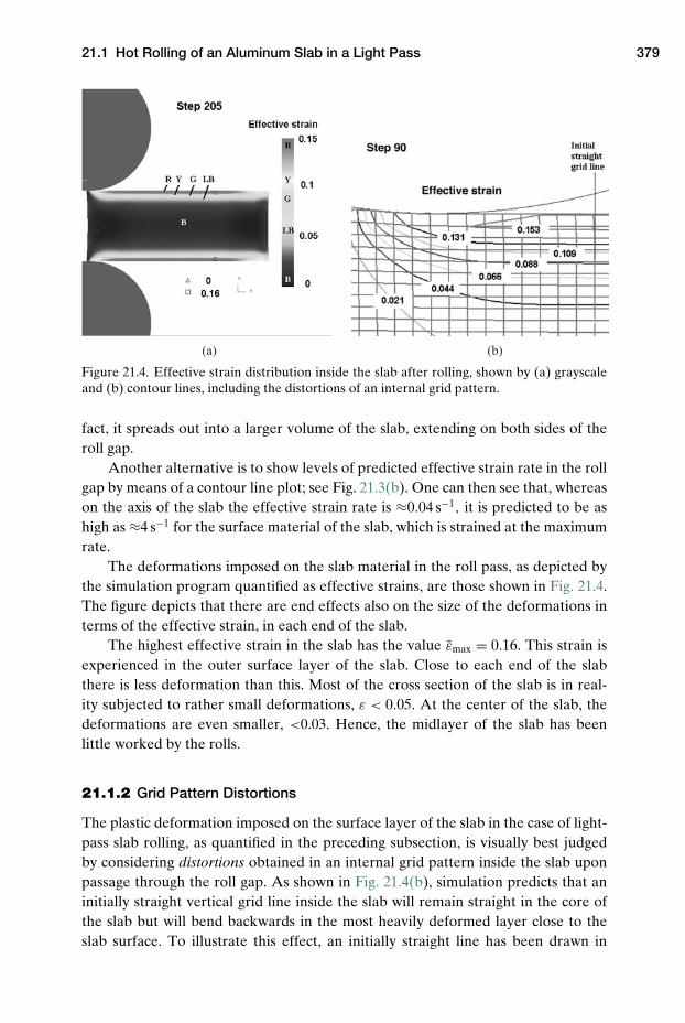
21.1 Hot Rolling of an Aluminum Slab in a Light Pass 379
(a) (b)
Figure 21.4. Effective strain distribution inside the slab after rolling, shown by (a) grayscaleand (b) contour lines, including the distortions of an internal grid pattern.
fact, it spreads out into a larger volume of the slab, extending on both sides of theroll gap.
Another alternative is to show levels of predicted effective strain rate in the rollgap by means of a contour line plot; see Fig. 21.3(b). One can then see that, whereason the axis of the slab the effective strain rate is ≈0.04 s−1, it is predicted to be ashigh as ≈4 s−1 for the surface material of the slab, which is strained at the maximumrate.
The deformations imposed on the slab material in the roll pass, as depicted bythe simulation program quantified as effective strains, are those shown in Fig. 21.4.The figure depicts that there are end effects also on the size of the deformations interms of the effective strain, in each end of the slab.
The highest effective strain in the slab has the value εmax = 0.16. This strain isexperienced in the outer surface layer of the slab. Close to each end of the slabthere is less deformation than this. Most of the cross section of the slab is in real-ity subjected to rather small deformations, ε < 0.05. At the center of the slab, thedeformations are even smaller, <0.03. Hence, the midlayer of the slab has beenlittle worked by the rolls.
21.1.2 Grid Pattern Distortions
The plastic deformation imposed on the surface layer of the slab in the case of light-pass slab rolling, as quantified in the preceding subsection, is visually best judgedby considering distortions obtained in an internal grid pattern inside the slab uponpassage through the roll gap. As shown in Fig. 21.4(b), simulation predicts that aninitially straight vertical grid line inside the slab will remain straight in the core ofthe slab but will bend backwards in the most heavily deformed layer close to theslab surface. To illustrate this effect, an initially straight line has been drawn in
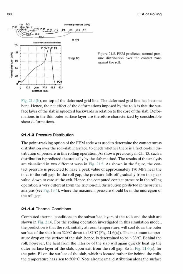
380 FEA of Rolling
Figure 21.5. FEM-predicted normal pres-sure distribution over the contact zoneagainst the roll.
Fig. 21.4(b), on top of the deformed grid line. The deformed grid line has becomebent. Hence, the net effect of the deformations imposed by the rolls is that the sur-face layer of the slab is squeezed backwards in relation to the core of the slab. Defor-mations in the thin outer surface layer are therefore characterized by considerableshear deformations.
21.1.3 Pressure Distribution
The point-tracking option of the FEM code was used to determine the contact stressdistribution over the roll–slab interface, to check whether there is a friction-hill dis-tribution of pressure in this rolling operation. As shown previously in Ch. 13, such adistribution is predicted theoretically by the slab method. The results of the analysisare visualized in two different ways in Fig. 21.5. As shown in the figure, the con-tact pressure is predicted to have a peak value of approximately 170 MPa near theinlet to the roll gap. In the roll gap, the pressure falls off gradually from this peakvalue, down to zero at the exit. Hence, the computed contact pressure in the rollingoperation is very different from the friction-hill distribution predicted in theoreticalanalysis (see Fig. 13.4), where the maximum pressure should be in the midregion ofthe roll gap.
21.1.4 Thermal Conditions
Computed thermal conditions in the subsurface layers of the rolls and the slab areshown in Fig. 21.6. For the rolling operation investigated in this simulation model,the prediction is that the roll, initially at room temperature, will cool down the outersurface of the slab from 520◦C down to 487◦C (Fig. 21.6(a)). The maximum temper-ature drop on the surface of the slab, hence, is determined to be ∼33◦C. Behind theroll, however, the heat from the interior of the slab will again quickly heat up theouter surface layer of the slab, upon exit from the roll gap. So in Fig. 21.6(a), forthe point P1 on the surface of the slab, which is located rather far behind the rolls,the temperature has risen to 508◦C. Note also thermal distribution along the surface
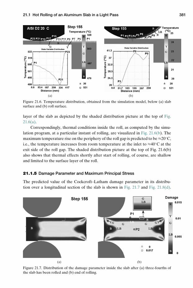
21.1 Hot Rolling of an Aluminum Slab in a Light Pass 381
(a) (b)
Figure 21.6. Temperature distribution, obtained from the simulation model, below (a) slabsurface and (b) roll surface.
layer of the slab as depicted by the shaded distribution picture at the top of Fig.21.6(a).
Correspondingly, thermal conditions inside the roll, as computed by the simu-lation program, at a particular instant of rolling, are visualized in Fig. 21.6(b). Themaximum temperature rise on the periphery of the roll gap is predicted to be ≈20◦C,i.e., the temperature increases from room temperature at the inlet to ≈40◦C at theexit side of the roll gap. The shaded distribution picture at the top of Fig. 21.6(b)also shows that thermal effects shortly after start of rolling, of course, are shallowand limited to the surface layer of the roll.
21.1.5 Damage Parameter and Maximum Principal Stress
The predicted value of the Cockcroft–Latham damage parameter in its distribu-tion over a longitudinal section of the slab is shown in Fig. 21.7 and Fig. 21.8(d).
(a) (b)
Figure 21.7. Distribution of the damage parameter inside the slab after (a) three-fourths ofthe slab has been rolled and (b) end of rolling.
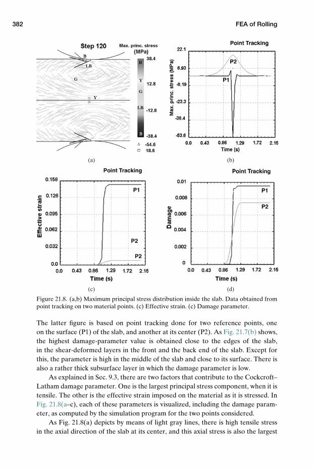
382 FEA of Rolling
(a)
(c)
(b)
(d)
Figure 21.8. (a,b) Maximum principal stress distribution inside the slab. Data obtained frompoint tracking on two material points. (c) Effective strain. (c) Damage parameter.
The latter figure is based on point tracking done for two reference points, oneon the surface (P1) of the slab, and another at its center (P2). As Fig. 21.7(b) shows,the highest damage-parameter value is obtained close to the edges of the slab,in the shear-deformed layers in the front and the back end of the slab. Except forthis, the parameter is high in the middle of the slab and close to its surface. There isalso a rather thick subsurface layer in which the damage parameter is low.
As explained in Sec. 9.3, there are two factors that contribute to the Cockcroft–Latham damage parameter. One is the largest principal stress component, when it istensile. The other is the effective strain imposed on the material as it is stressed. InFig. 21.8(a–c), each of these parameters is visualized, including the damage param-eter, as computed by the simulation program for the two points considered.
As Fig. 21.8(a) depicts by means of light gray lines, there is high tensile stressin the axial direction of the slab at its center, and this axial stress is also the largest
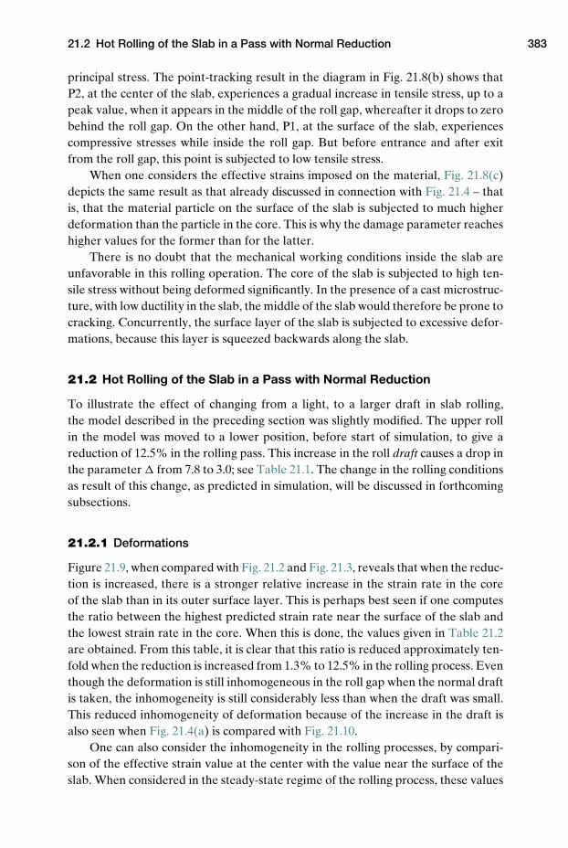
21.2 Hot Rolling of the Slab in a Pass with Normal Reduction 383
principal stress. The point-tracking result in the diagram in Fig. 21.8(b) shows thatP2, at the center of the slab, experiences a gradual increase in tensile stress, up to apeak value, when it appears in the middle of the roll gap, whereafter it drops to zerobehind the roll gap. On the other hand, P1, at the surface of the slab, experiencescompressive stresses while inside the roll gap. But before entrance and after exitfrom the roll gap, this point is subjected to low tensile stress.
When one considers the effective strains imposed on the material, Fig. 21.8(c)depicts the same result as that already discussed in connection with Fig. 21.4 – thatis, that the material particle on the surface of the slab is subjected to much higherdeformation than the particle in the core. This is why the damage parameter reacheshigher values for the former than for the latter.
There is no doubt that the mechanical working conditions inside the slab areunfavorable in this rolling operation. The core of the slab is subjected to high ten-sile stress without being deformed significantly. In the presence of a cast microstruc-ture, with low ductility in the slab, the middle of the slab would therefore be prone tocracking. Concurrently, the surface layer of the slab is subjected to excessive defor-mations, because this layer is squeezed backwards along the slab.
21.2 Hot Rolling of the Slab in a Pass with Normal Reduction
To illustrate the effect of changing from a light, to a larger draft in slab rolling,the model described in the preceding section was slightly modified. The upper rollin the model was moved to a lower position, before start of simulation, to give areduction of 12.5% in the rolling pass. This increase in the roll draft causes a drop inthe parameter � from 7.8 to 3.0; see Table 21.1. The change in the rolling conditionsas result of this change, as predicted in simulation, will be discussed in forthcomingsubsections.
21.2.1 Deformations
Figure 21.9, when compared with Fig. 21.2 and Fig. 21.3, reveals that when the reduc-tion is increased, there is a stronger relative increase in the strain rate in the coreof the slab than in its outer surface layer. This is perhaps best seen if one computesthe ratio between the highest predicted strain rate near the surface of the slab andthe lowest strain rate in the core. When this is done, the values given in Table 21.2are obtained. From this table, it is clear that this ratio is reduced approximately ten-fold when the reduction is increased from 1.3% to 12.5% in the rolling process. Eventhough the deformation is still inhomogeneous in the roll gap when the normal draftis taken, the inhomogeneity is still considerably less than when the draft was small.This reduced inhomogeneity of deformation because of the increase in the draft isalso seen when Fig. 21.4(a) is compared with Fig. 21.10.
One can also consider the inhomogeneity in the rolling processes, by compari-son of the effective strain value at the center with the value near the surface of theslab. When considered in the steady-state regime of the rolling process, these values
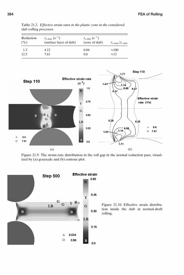
384 FEA of Rolling
Table 21.2. Effective strain rates in the plastic zone in the consideredslab rolling processes
Reduction εe,max (s−1) εe,min (s−1)(%) (surface layer of slab) (core of slab) εe,max/εe,min
1.3 4.12 0.04 ≈10012.5 7.61 0.6 ≈13
(a) (b)
Figure 21.9. The strain-rate distribution in the roll gap in the normal reduction pass, visual-ized by (a) grayscale and (b) contour plot.
Figure 21.10. Effective strain distribu-tion inside the slab in normal-draftrolling.
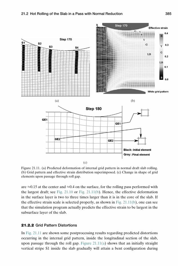
21.2 Hot Rolling of the Slab in a Pass with Normal Reduction 385
(a) (b)
(c)
Figure 21.11. (a) Predicted deformation of internal grid pattern in normal draft slab rolling.(b) Grid pattern and effective strain distribution superimposed. (c) Change in shape of gridelements upon passage through roll gap.
are ≈0.15 at the center and ≈0.4 on the surface, for the rolling pass performed withthe largest draft; see Fig. 21.10 or Fig. 21.11(b). Hence, the effective deformationin the surface layer is two to three times larger than it is in the core of the slab. Ifthe effective strain scale is selected properly, as shown in Fig. 21.11(b), one can seethat the simulation program actually predicts the effective strain to be largest in thesubsurface layer of the slab.
21.2.2 Grid Pattern Distortions
In Fig. 21.11 are shown some postprocessing results regarding predicted distortionsoccurring in the internal grid pattern, inside the longitudinal section of the slab,upon passage through the roll gap. Figure 21.11(a) shows that an initially straightvertical stripe S1 inside the slab gradually will attain a bent configuration during
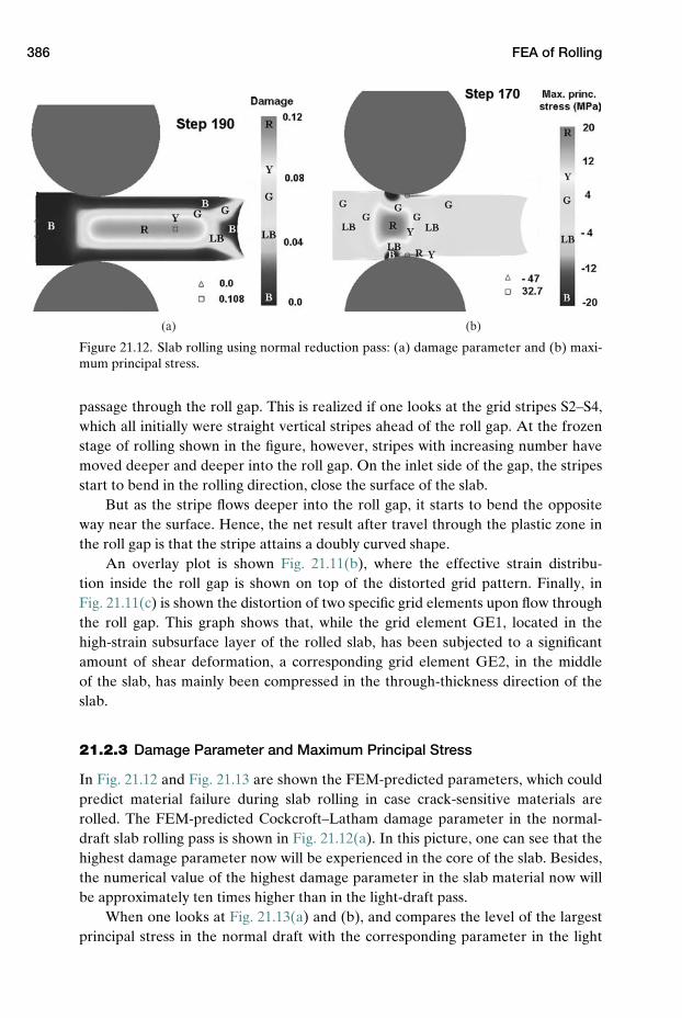
386 FEA of Rolling
(a) (b)
Figure 21.12. Slab rolling using normal reduction pass: (a) damage parameter and (b) maxi-mum principal stress.
passage through the roll gap. This is realized if one looks at the grid stripes S2–S4,which all initially were straight vertical stripes ahead of the roll gap. At the frozenstage of rolling shown in the figure, however, stripes with increasing number havemoved deeper and deeper into the roll gap. On the inlet side of the gap, the stripesstart to bend in the rolling direction, close the surface of the slab.
But as the stripe flows deeper into the roll gap, it starts to bend the oppositeway near the surface. Hence, the net result after travel through the plastic zone inthe roll gap is that the stripe attains a doubly curved shape.
An overlay plot is shown Fig. 21.11(b), where the effective strain distribu-tion inside the roll gap is shown on top of the distorted grid pattern. Finally, inFig. 21.11(c) is shown the distortion of two specific grid elements upon flow throughthe roll gap. This graph shows that, while the grid element GE1, located in thehigh-strain subsurface layer of the rolled slab, has been subjected to a significantamount of shear deformation, a corresponding grid element GE2, in the middleof the slab, has mainly been compressed in the through-thickness direction of theslab.
21.2.3 Damage Parameter and Maximum Principal Stress
In Fig. 21.12 and Fig. 21.13 are shown the FEM-predicted parameters, which couldpredict material failure during slab rolling in case crack-sensitive materials arerolled. The FEM-predicted Cockcroft–Latham damage parameter in the normal-draft slab rolling pass is shown in Fig. 21.12(a). In this picture, one can see that thehighest damage parameter now will be experienced in the core of the slab. Besides,the numerical value of the highest damage parameter in the slab material now willbe approximately ten times higher than in the light-draft pass.
When one looks at Fig. 21.13(a) and (b), and compares the level of the largestprincipal stress in the normal draft with the corresponding parameter in the light
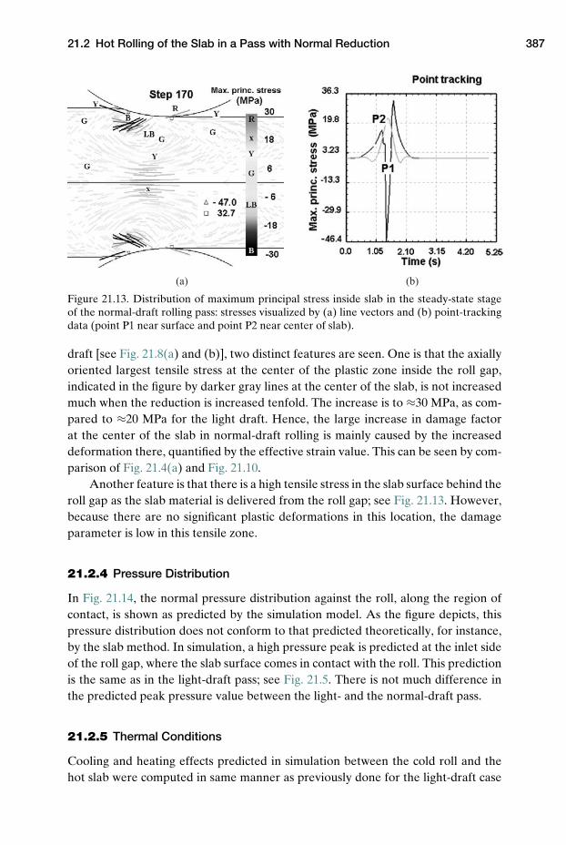
21.2 Hot Rolling of the Slab in a Pass with Normal Reduction 387
(a) (b)
Figure 21.13. Distribution of maximum principal stress inside slab in the steady-state stageof the normal-draft rolling pass: stresses visualized by (a) line vectors and (b) point-trackingdata (point P1 near surface and point P2 near center of slab).
draft [see Fig. 21.8(a) and (b)], two distinct features are seen. One is that the axiallyoriented largest tensile stress at the center of the plastic zone inside the roll gap,indicated in the figure by darker gray lines at the center of the slab, is not increasedmuch when the reduction is increased tenfold. The increase is to ≈30 MPa, as com-pared to ≈20 MPa for the light draft. Hence, the large increase in damage factorat the center of the slab in normal-draft rolling is mainly caused by the increaseddeformation there, quantified by the effective strain value. This can be seen by com-parison of Fig. 21.4(a) and Fig. 21.10.
Another feature is that there is a high tensile stress in the slab surface behind theroll gap as the slab material is delivered from the roll gap; see Fig. 21.13. However,because there are no significant plastic deformations in this location, the damageparameter is low in this tensile zone.
21.2.4 Pressure Distribution
In Fig. 21.14, the normal pressure distribution against the roll, along the region ofcontact, is shown as predicted by the simulation model. As the figure depicts, thispressure distribution does not conform to that predicted theoretically, for instance,by the slab method. In simulation, a high pressure peak is predicted at the inlet sideof the roll gap, where the slab surface comes in contact with the roll. This predictionis the same as in the light-draft pass; see Fig. 21.5. There is not much difference inthe predicted peak pressure value between the light- and the normal-draft pass.
21.2.5 Thermal Conditions
Cooling and heating effects predicted in simulation between the cold roll and thehot slab were computed in same manner as previously done for the light-draft case
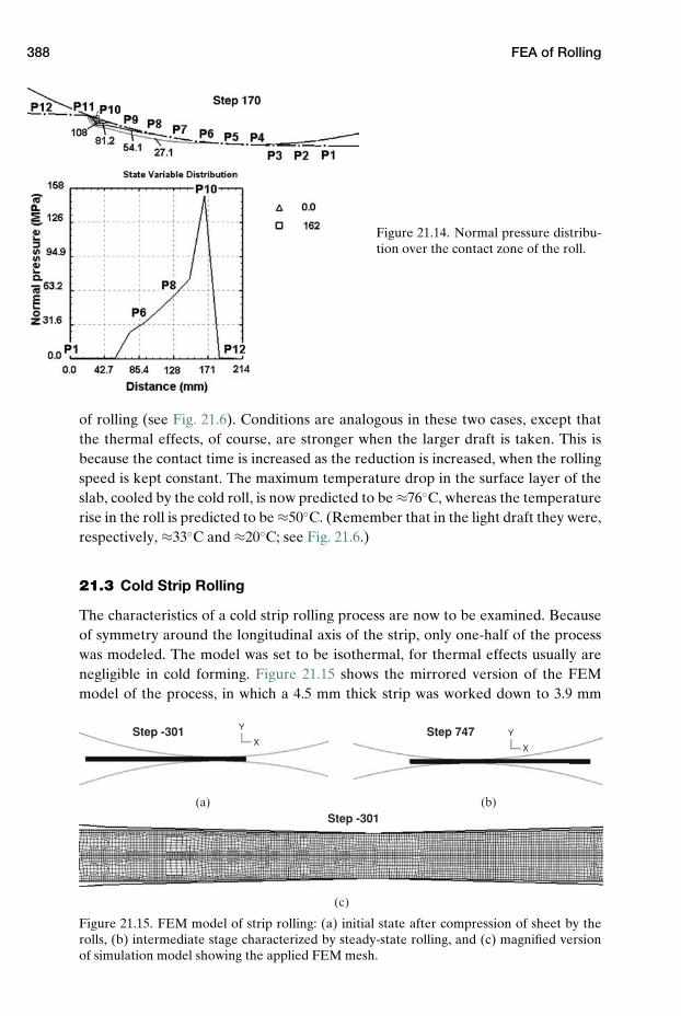
388 FEA of Rolling
Figure 21.14. Normal pressure distribu-tion over the contact zone of the roll.
of rolling (see Fig. 21.6). Conditions are analogous in these two cases, except thatthe thermal effects, of course, are stronger when the larger draft is taken. This isbecause the contact time is increased as the reduction is increased, when the rollingspeed is kept constant. The maximum temperature drop in the surface layer of theslab, cooled by the cold roll, is now predicted to be ≈76◦C, whereas the temperaturerise in the roll is predicted to be ≈50◦C. (Remember that in the light draft they were,respectively, ≈33◦C and ≈20◦C; see Fig. 21.6.)
21.3 Cold Strip Rolling
The characteristics of a cold strip rolling process are now to be examined. Becauseof symmetry around the longitudinal axis of the strip, only one-half of the processwas modeled. The model was set to be isothermal, for thermal effects usually arenegligible in cold forming. Figure 21.15 shows the mirrored version of the FEMmodel of the process, in which a 4.5 mm thick strip was worked down to 3.9 mm
(a) (b)
(c)
X
Y
X
YStep -301
Step -301
Step 747
Figure 21.15. FEM model of strip rolling: (a) initial state after compression of sheet by therolls, (b) intermediate stage characterized by steady-state rolling, and (c) magnified versionof simulation model showing the applied FEM mesh.
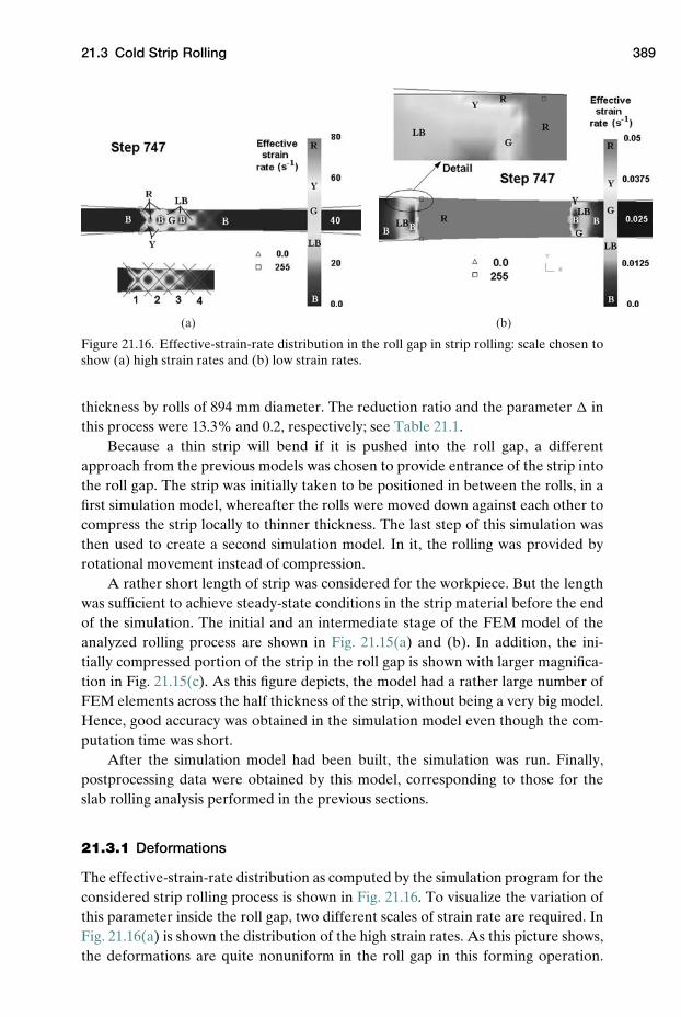
21.3 Cold Strip Rolling 389
(a) (b)
Figure 21.16. Effective-strain-rate distribution in the roll gap in strip rolling: scale chosen toshow (a) high strain rates and (b) low strain rates.
thickness by rolls of 894 mm diameter. The reduction ratio and the parameter � inthis process were 13.3% and 0.2, respectively; see Table 21.1.
Because a thin strip will bend if it is pushed into the roll gap, a differentapproach from the previous models was chosen to provide entrance of the strip intothe roll gap. The strip was initially taken to be positioned in between the rolls, in afirst simulation model, whereafter the rolls were moved down against each other tocompress the strip locally to thinner thickness. The last step of this simulation wasthen used to create a second simulation model. In it, the rolling was provided byrotational movement instead of compression.
A rather short length of strip was considered for the workpiece. But the lengthwas sufficient to achieve steady-state conditions in the strip material before the endof the simulation. The initial and an intermediate stage of the FEM model of theanalyzed rolling process are shown in Fig. 21.15(a) and (b). In addition, the ini-tially compressed portion of the strip in the roll gap is shown with larger magnifica-tion in Fig. 21.15(c). As this figure depicts, the model had a rather large number ofFEM elements across the half thickness of the strip, without being a very big model.Hence, good accuracy was obtained in the simulation model even though the com-putation time was short.
After the simulation model had been built, the simulation was run. Finally,postprocessing data were obtained by this model, corresponding to those for theslab rolling analysis performed in the previous sections.
21.3.1 Deformations
The effective-strain-rate distribution as computed by the simulation program for theconsidered strip rolling process is shown in Fig. 21.16. To visualize the variation ofthis parameter inside the roll gap, two different scales of strain rate are required. InFig. 21.16(a) is shown the distribution of the high strain rates. As this picture shows,the deformations are quite nonuniform in the roll gap in this forming operation.
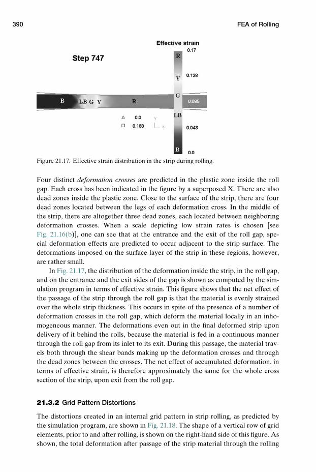
390 FEA of Rolling
Figure 21.17. Effective strain distribution in the strip during rolling.
Four distinct deformation crosses are predicted in the plastic zone inside the rollgap. Each cross has been indicated in the figure by a superposed X. There are alsodead zones inside the plastic zone. Close to the surface of the strip, there are fourdead zones located between the legs of each deformation cross. In the middle ofthe strip, there are altogether three dead zones, each located between neighboringdeformation crosses. When a scale depicting low strain rates is chosen [seeFig. 21.16(b)], one can see that at the entrance and the exit of the roll gap, spe-cial deformation effects are predicted to occur adjacent to the strip surface. Thedeformations imposed on the surface layer of the strip in these regions, however,are rather small.
In Fig. 21.17, the distribution of the deformation inside the strip, in the roll gap,and on the entrance and the exit sides of the gap is shown as computed by the sim-ulation program in terms of effective strain. This figure shows that the net effect ofthe passage of the strip through the roll gap is that the material is evenly strainedover the whole strip thickness. This occurs in spite of the presence of a number ofdeformation crosses in the roll gap, which deform the material locally in an inho-mogeneous manner. The deformations even out in the final deformed strip upondelivery of it behind the rolls, because the material is fed in a continuous mannerthrough the roll gap from its inlet to its exit. During this passage, the material trav-els both through the shear bands making up the deformation crosses and throughthe dead zones between the crosses. The net effect of accumulated deformation, interms of effective strain, is therefore approximately the same for the whole crosssection of the strip, upon exit from the roll gap.
21.3.2 Grid Pattern Distortions
The distortions created in an internal grid pattern in strip rolling, as predicted bythe simulation program, are shown in Fig. 21.18. The shape of a vertical row of gridelements, prior to and after rolling, is shown on the right-hand side of this figure. Asshown, the total deformation after passage of the strip material through the rolling
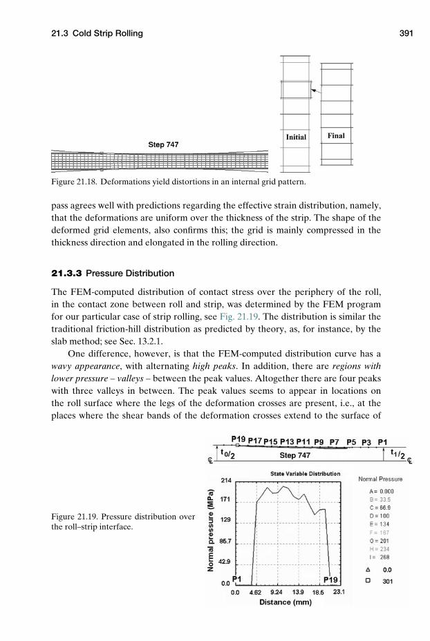
21.3 Cold Strip Rolling 391
Figure 21.18. Deformations yield distortions in an internal grid pattern.
pass agrees well with predictions regarding the effective strain distribution, namely,that the deformations are uniform over the thickness of the strip. The shape of thedeformed grid elements, also confirms this; the grid is mainly compressed in thethickness direction and elongated in the rolling direction.
21.3.3 Pressure Distribution
The FEM-computed distribution of contact stress over the periphery of the roll,in the contact zone between roll and strip, was determined by the FEM programfor our particular case of strip rolling, see Fig. 21.19. The distribution is similar thetraditional friction-hill distribution as predicted by theory, as, for instance, by theslab method; see Sec. 13.2.1.
One difference, however, is that the FEM-computed distribution curve has awavy appearance, with alternating high peaks. In addition, there are regions withlower pressure – valleys – between the peak values. Altogether there are four peakswith three valleys in between. The peak values seems to appear in locations onthe roll surface where the legs of the deformation crosses are present, i.e., at theplaces where the shear bands of the deformation crosses extend to the surface of
Figure 21.19. Pressure distribution overthe roll–strip interface.
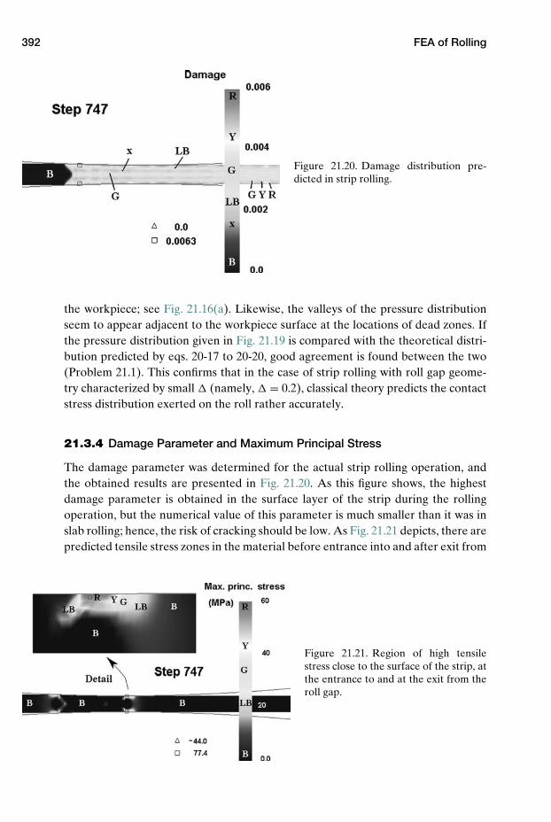
392 FEA of Rolling
Figure 21.20. Damage distribution pre-dicted in strip rolling.
the workpiece; see Fig. 21.16(a). Likewise, the valleys of the pressure distributionseem to appear adjacent to the workpiece surface at the locations of dead zones. Ifthe pressure distribution given in Fig. 21.19 is compared with the theoretical distri-bution predicted by eqs. 20-17 to 20-20, good agreement is found between the two(Problem 21.1). This confirms that in the case of strip rolling with roll gap geome-try characterized by small � (namely, � = 0.2), classical theory predicts the contactstress distribution exerted on the roll rather accurately.
21.3.4 Damage Parameter and Maximum Principal Stress
The damage parameter was determined for the actual strip rolling operation, andthe obtained results are presented in Fig. 21.20. As this figure shows, the highestdamage parameter is obtained in the surface layer of the strip during the rollingoperation, but the numerical value of this parameter is much smaller than it was inslab rolling; hence, the risk of cracking should be low. As Fig. 21.21 depicts, there arepredicted tensile stress zones in the material before entrance into and after exit from
Figure 21.21. Region of high tensilestress close to the surface of the strip, atthe entrance to and at the exit from theroll gap.
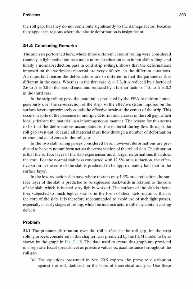
Problems 393
the roll gap, but they do not contribute significantly to the damage factor, becausethey appear in regions where the plastic deformation is insignificant.
21.4 Concluding Remarks
The analysis performed here, where three different cases of rolling were considered(namely, a light-reduction pass and a normal-reduction pass in hot slab rolling, andfinally a normal-reduction pass in cold strip rolling), shows that the deformationsimposed on the workpiece material are very different in the different situations.An important reason the deformations are so different is that the parameter � isdifferent in the cases. Whereas in the first case � = 7.8, it is reduced by a factor of2.6 to � = 3.0 in the second case, and reduced by a further factor of 15, to � = 0.2in the third case.
In the strip rolling pass, the material is predicted by the FEA to deform homo-geneously over the cross section of the strip, so the effective strain imposed on thesurface layer approximately equals the effective strain at the center of the strip. Thisoccurs in spite of the presence of multiple deformation crosses in the roll gap, whichlocally deform the material in a inhomogeneous manner. The reason for this seemsto be that the deformations accumulated in the material during flow through theroll gap even out, because all material must flow through a number of deformationcrosses and dead zones in the roll gap.
In the two slab rolling passes considered here, however, deformations are pre-dicted to be very nonuniform across the cross section of the rolled slab. The situationis that the surface layer of the slab experiences much larger deformations than doesthe core. For the normal slab pass conducted with 12.5% area reduction, the effec-tive strain in the core of the slab is predicted to be approximately half that in thesurface layer.
In the low-reduction slab pass, where there is only 1.3% area reduction, the sur-face layer of the slab is predicted to be squeezed backwards in relation to the coreof the slab, which is indeed very lightly worked. The surface of the slab is there-fore subjected to much higher strains, in the form of shear deformations, than isthe core of the slab. It is therefore recommended to avoid use of such light passes,especially in early stages of rolling, while the microstructure still may contain castingdefects.
Problem
21.1 The pressure distribution over the roll surface in the roll gap, for the striprolling process considered in this chapter, was predicted by the FEM model to be asshown by the graph in Fig. 21.19. The data used to create this graph are providedin a separate Excel spreadsheet as pressure values vs. axial distance throughout theroll gap.
(a) The equations presented in Sec. 20.5 express the pressure distributionagainst the roll, deduced on the basis of theoretical analysis. Use these

394 FEA of Rolling
equations to determine the pressure distribution in this case. For compari-son make an overlay plot of the pressure distribution computed by theoryand the corresponding results from FEA.
(b) Discuss how well the theoretical pressure distribution agrees with the cor-responding distribution obtained in the FEA.
REFERENCE
Bakken, A.: “FEM-modelling as tool for optimisation of cold and hot rolling processes,”M.Sc. thesis, Norwegian Institute of Science and Technology (NTNU), 2005 (in Norwe-gian).
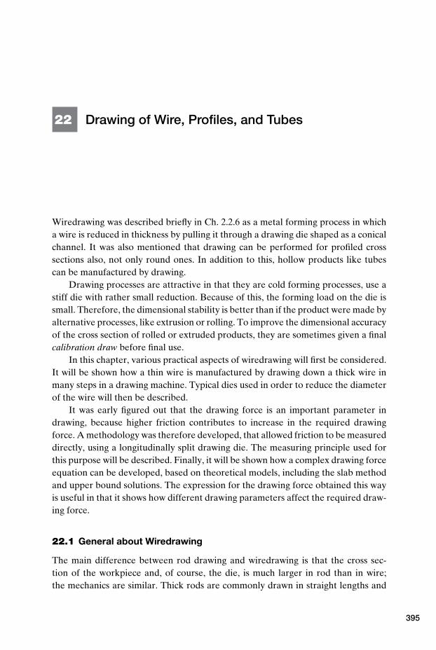
22 Drawing of Wire, Profiles, and Tubes
Wiredrawing was described briefly in Ch. 2.2.6 as a metal forming process in whicha wire is reduced in thickness by pulling it through a drawing die shaped as a conicalchannel. It was also mentioned that drawing can be performed for profiled crosssections also, not only round ones. In addition to this, hollow products like tubescan be manufactured by drawing.
Drawing processes are attractive in that they are cold forming processes, use astiff die with rather small reduction. Because of this, the forming load on the die issmall. Therefore, the dimensional stability is better than if the product were made byalternative processes, like extrusion or rolling. To improve the dimensional accuracyof the cross section of rolled or extruded products, they are sometimes given a finalcalibration draw before final use.
In this chapter, various practical aspects of wiredrawing will first be considered.It will be shown how a thin wire is manufactured by drawing down a thick wire inmany steps in a drawing machine. Typical dies used in order to reduce the diameterof the wire will then be described.
It was early figured out that the drawing force is an important parameter indrawing, because higher friction contributes to increase in the required drawingforce. A methodology was therefore developed, that allowed friction to be measureddirectly, using a longitudinally split drawing die. The measuring principle used forthis purpose will be described. Finally, it will be shown how a complex drawing forceequation can be developed, based on theoretical models, including the slab methodand upper bound solutions. The expression for the drawing force obtained this wayis useful in that it shows how different drawing parameters affect the required draw-ing force.
22.1 General about Wiredrawing
The main difference between rod drawing and wiredrawing is that the cross sec-tion of the workpiece and, of course, the die, is much larger in rod than in wire;the mechanics are similar. Thick rods are commonly drawn in straight lengths and
395
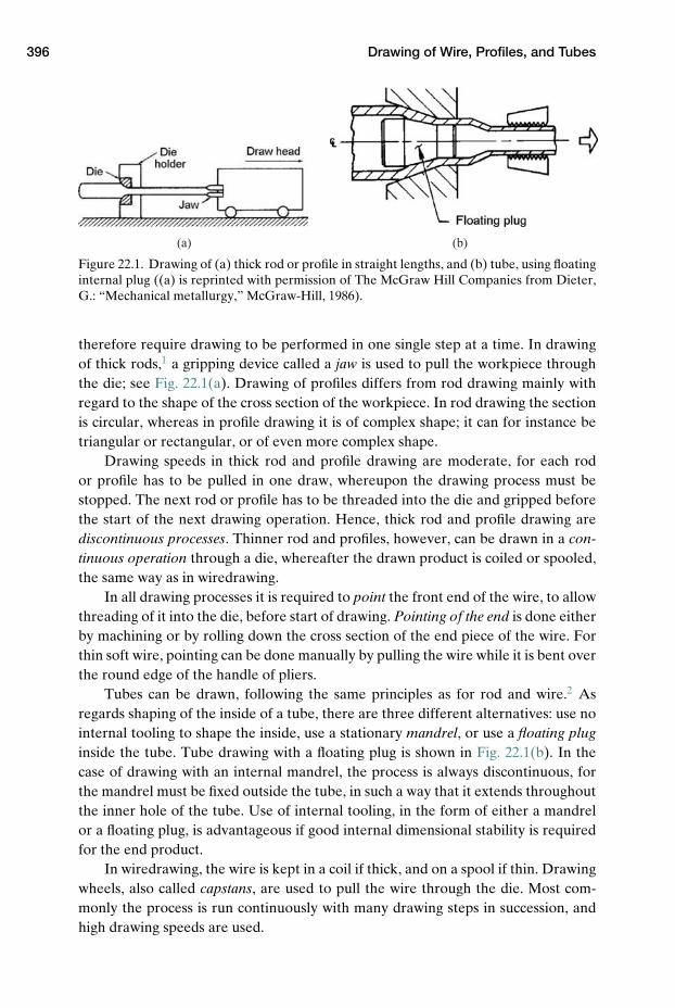
396 Drawing of Wire, Profiles, and Tubes
(a) (b)
Figure 22.1. Drawing of (a) thick rod or profile in straight lengths, and (b) tube, using floatinginternal plug ((a) is reprinted with permission of The McGraw Hill Companies from Dieter,G.: “Mechanical metallurgy,” McGraw-Hill, 1986).
therefore require drawing to be performed in one single step at a time. In drawingof thick rods,1 a gripping device called a jaw is used to pull the workpiece throughthe die; see Fig. 22.1(a). Drawing of profiles differs from rod drawing mainly withregard to the shape of the cross section of the workpiece. In rod drawing the sectionis circular, whereas in profile drawing it is of complex shape; it can for instance betriangular or rectangular, or of even more complex shape.
Drawing speeds in thick rod and profile drawing are moderate, for each rodor profile has to be pulled in one draw, whereupon the drawing process must bestopped. The next rod or profile has to be threaded into the die and gripped beforethe start of the next drawing operation. Hence, thick rod and profile drawing arediscontinuous processes. Thinner rod and profiles, however, can be drawn in a con-tinuous operation through a die, whereafter the drawn product is coiled or spooled,the same way as in wiredrawing.
In all drawing processes it is required to point the front end of the wire, to allowthreading of it into the die, before start of drawing. Pointing of the end is done eitherby machining or by rolling down the cross section of the end piece of the wire. Forthin soft wire, pointing can be done manually by pulling the wire while it is bent overthe round edge of the handle of pliers.
Tubes can be drawn, following the same principles as for rod and wire.2 Asregards shaping of the inside of a tube, there are three different alternatives: use nointernal tooling to shape the inside, use a stationary mandrel, or use a floating pluginside the tube. Tube drawing with a floating plug is shown in Fig. 22.1(b). In thecase of drawing with an internal mandrel, the process is always discontinuous, forthe mandrel must be fixed outside the tube, in such a way that it extends throughoutthe inner hole of the tube. Use of internal tooling, in the form of either a mandrelor a floating plug, is advantageous if good internal dimensional stability is requiredfor the end product.
In wiredrawing, the wire is kept in a coil if thick, and on a spool if thin. Drawingwheels, also called capstans, are used to pull the wire through the die. Most com-monly the process is run continuously with many drawing steps in succession, andhigh drawing speeds are used.
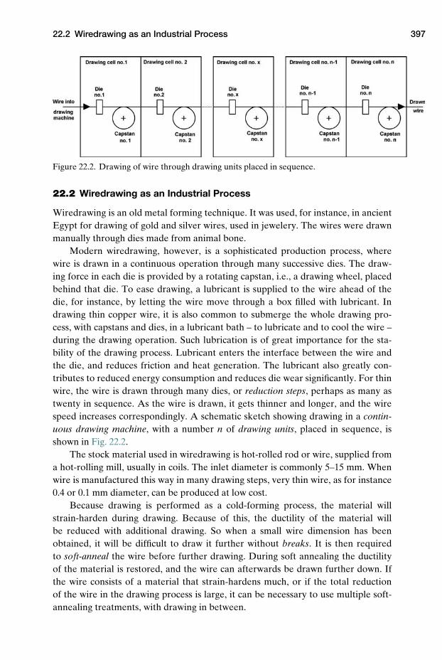
22.2 Wiredrawing as an Industrial Process 397
Figure 22.2. Drawing of wire through drawing units placed in sequence.
22.2 Wiredrawing as an Industrial Process
Wiredrawing is an old metal forming technique. It was used, for instance, in ancientEgypt for drawing of gold and silver wires, used in jewelery. The wires were drawnmanually through dies made from animal bone.
Modern wiredrawing, however, is a sophisticated production process, wherewire is drawn in a continuous operation through many successive dies. The draw-ing force in each die is provided by a rotating capstan, i.e., a drawing wheel, placedbehind that die. To ease drawing, a lubricant is supplied to the wire ahead of thedie, for instance, by letting the wire move through a box filled with lubricant. Indrawing thin copper wire, it is also common to submerge the whole drawing pro-cess, with capstans and dies, in a lubricant bath – to lubricate and to cool the wire –during the drawing operation. Such lubrication is of great importance for the sta-bility of the drawing process. Lubricant enters the interface between the wire andthe die, and reduces friction and heat generation. The lubricant also greatly con-tributes to reduced energy consumption and reduces die wear significantly. For thinwire, the wire is drawn through many dies, or reduction steps, perhaps as many astwenty in sequence. As the wire is drawn, it gets thinner and longer, and the wirespeed increases correspondingly. A schematic sketch showing drawing in a contin-uous drawing machine, with a number n of drawing units, placed in sequence, isshown in Fig. 22.2.
The stock material used in wiredrawing is hot-rolled rod or wire, supplied froma hot-rolling mill, usually in coils. The inlet diameter is commonly 5–15 mm. Whenwire is manufactured this way in many drawing steps, very thin wire, as for instance0.4 or 0.1 mm diameter, can be produced at low cost.
Because drawing is performed as a cold-forming process, the material willstrain-harden during drawing. Because of this, the ductility of the material willbe reduced with additional drawing. So when a small wire dimension has beenobtained, it will be difficult to draw it further without breaks. It is then requiredto soft-anneal the wire before further drawing. During soft annealing the ductilityof the material is restored, and the wire can afterwards be drawn further down. Ifthe wire consists of a material that strain-hardens much, or if the total reductionof the wire in the drawing process is large, it can be necessary to use multiple soft-annealing treatments, with drawing in between.
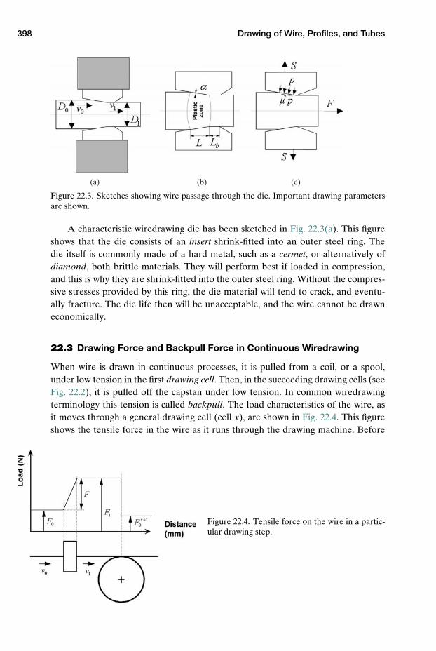
398 Drawing of Wire, Profiles, and Tubes
(a) (b) (c)
Figure 22.3. Sketches showing wire passage through the die. Important drawing parametersare shown.
A characteristic wiredrawing die has been sketched in Fig. 22.3(a). This figureshows that the die consists of an insert shrink-fitted into an outer steel ring. Thedie itself is commonly made of a hard metal, such as a cermet, or alternatively ofdiamond, both brittle materials. They will perform best if loaded in compression,and this is why they are shrink-fitted into the outer steel ring. Without the compres-sive stresses provided by this ring, the die material will tend to crack, and eventu-ally fracture. The die life then will be unacceptable, and the wire cannot be drawneconomically.
22.3 Drawing Force and Backpull Force in Continuous Wiredrawing
When wire is drawn in continuous processes, it is pulled from a coil, or a spool,under low tension in the first drawing cell. Then, in the succeeding drawing cells (seeFig. 22.2), it is pulled off the capstan under low tension. In common wiredrawingterminology this tension is called backpull. The load characteristics of the wire, asit moves through a general drawing cell (cell x), are shown in Fig. 22.4. This figureshows the tensile force in the wire as it runs through the drawing machine. Before
Figure 22.4. Tensile force on the wire in a partic-ular drawing step.
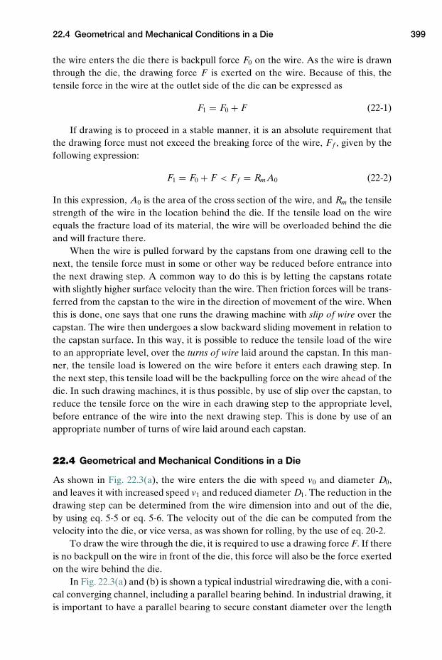
22.4 Geometrical and Mechanical Conditions in a Die 399
the wire enters the die there is backpull force F0 on the wire. As the wire is drawnthrough the die, the drawing force F is exerted on the wire. Because of this, thetensile force in the wire at the outlet side of the die can be expressed as
F1 = F0 + F (22-1)
If drawing is to proceed in a stable manner, it is an absolute requirement thatthe drawing force must not exceed the breaking force of the wire, F f , given by thefollowing expression:
F1 = F0 + F < Ff = Rm A0 (22-2)
In this expression, A0 is the area of the cross section of the wire, and Rm the tensilestrength of the wire in the location behind the die. If the tensile load on the wireequals the fracture load of its material, the wire will be overloaded behind the dieand will fracture there.
When the wire is pulled forward by the capstans from one drawing cell to thenext, the tensile force must in some or other way be reduced before entrance intothe next drawing step. A common way to do this is by letting the capstans rotatewith slightly higher surface velocity than the wire. Then friction forces will be trans-ferred from the capstan to the wire in the direction of movement of the wire. Whenthis is done, one says that one runs the drawing machine with slip of wire over thecapstan. The wire then undergoes a slow backward sliding movement in relation tothe capstan surface. In this way, it is possible to reduce the tensile load of the wireto an appropriate level, over the turns of wire laid around the capstan. In this man-ner, the tensile load is lowered on the wire before it enters each drawing step. Inthe next step, this tensile load will be the backpulling force on the wire ahead of thedie. In such drawing machines, it is thus possible, by use of slip over the capstan, toreduce the tensile force on the wire in each drawing step to the appropriate level,before entrance of the wire into the next drawing step. This is done by use of anappropriate number of turns of wire laid around each capstan.
22.4 Geometrical and Mechanical Conditions in a Die
As shown in Fig. 22.3(a), the wire enters the die with speed v0 and diameter D0,and leaves it with increased speed v1 and reduced diameter D1. The reduction in thedrawing step can be determined from the wire dimension into and out of the die,by using eq. 5-5 or eq. 5-6. The velocity out of the die can be computed from thevelocity into the die, or vice versa, as was shown for rolling, by the use of eq. 20-2.
To draw the wire through the die, it is required to use a drawing force F. If thereis no backpull on the wire in front of the die, this force will also be the force exertedon the wire behind the die.
In Fig. 22.3(a) and (b) is shown a typical industrial wiredrawing die, with a coni-cal converging channel, including a parallel bearing behind. In industrial drawing, itis important to have a parallel bearing to secure constant diameter over the length
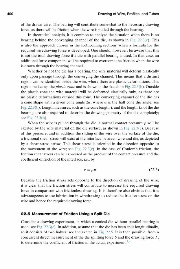
400 Drawing of Wire, Profiles, and Tubes
of the drawn wire. The bearing will contribute somewhat to the necessary drawingforce, as there will be friction when the wire is pulled through the bearing.
In theoretical analysis, it is common to analyze the situation when there is nobearing behind the converging channel of the die, as shown in Fig. 22.3(c). Thisis also the approach chosen in the forthcoming sections, when a formula for therequired wiredrawing force is developed. One should, however, be aware that thisis not the total drawing force if a die with parallel bearing is used. In that case, anadditional force component will be required to overcome the friction when the wireis drawn through the bearing channel.
Whether or not the die has a bearing, the wire material will deform plasticallyonly upon passage through the converging die channel. This means that a distinctregion can be identified inside the wire, where there are plastic deformations. Thisregion makes up the plastic zone and is shown in the sketch in Fig. 22.3(b). Outsidethe plastic zone the wire material will be deformed elastically only, as there areno plastic deformations outside this zone. The converging channel of the die hasa cone shape with a given cone angle 2α, where α is the half cone die angle; seeFig. 22.3(b). Length measures, such as the cone length L and the length Lb of the diebearing, are also required to describe the drawing geometry of the die completely;see Fig. 22.3(b).
When the wire is pulled through the die, a normal contact pressure p will beexerted by the wire material on the die surface, as shown in Fig. 22.3(c). Becauseof this pressure, and in addition the sliding of the wire over the surface of the die,a frictional shear stress will exist at the interface between wire and die, as depictedby a shear stress arrow. This shear stress is oriented in the direction opposite tothe movement of the wire; see Fig. 22.3(c). In the case of Coulomb friction, thefriction shear stress can be expressed as the product of the contact pressure and thecoefficient of friction of the interface, i.e., by
τ = µp (22-3)
Because the friction stress acts opposite to the direction of drawing of the wire,it is clear that the friction stress will contribute to increase the required drawingforce in comparison with frictionless drawing. It is therefore also obvious that it isadvantageous to use lubrication in wiredrawing to reduce the friction stress on thewire and hence the required drawing force.
22.5 Measurement of Friction Using a Split Die
Consider a drawing experiment, in which a conical die without parallel bearing isused; see Fig. 22.3(c). In addition, assume that the die has been split longitudinally,so it consists of two halves; see the sketch in Fig. 22.5. It is then possible, from aconcurrent direct measurement of the die splitting force S and the drawing force F ,to determine the coefficient of friction in the actual experiment.3,4
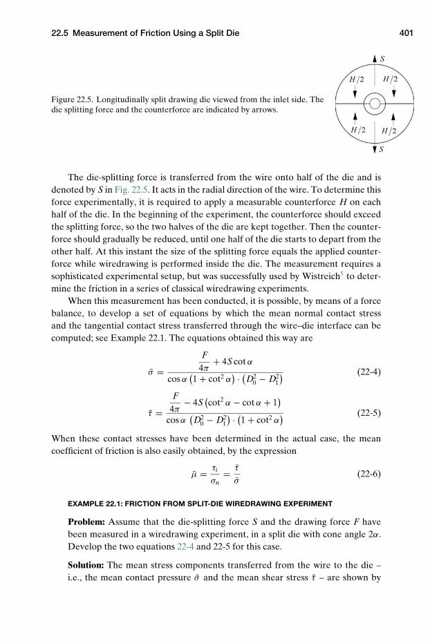
22.5 Measurement of Friction Using a Split Die 401
Figure 22.5. Longitudinally split drawing die viewed from the inlet side. Thedie splitting force and the counterforce are indicated by arrows.
The die-splitting force is transferred from the wire onto half of the die and isdenoted by S in Fig. 22.5. It acts in the radial direction of the wire. To determine thisforce experimentally, it is required to apply a measurable counterforce H on eachhalf of the die. In the beginning of the experiment, the counterforce should exceedthe splitting force, so the two halves of the die are kept together. Then the counter-force should gradually be reduced, until one half of the die starts to depart from theother half. At this instant the size of the splitting force equals the applied counter-force while wiredrawing is performed inside the die. The measurement requires asophisticated experimental setup, but was successfully used by Wistreich5 to deter-mine the friction in a series of classical wiredrawing experiments.
When this measurement has been conducted, it is possible, by means of a forcebalance, to develop a set of equations by which the mean normal contact stressand the tangential contact stress transferred through the wire–die interface can becomputed; see Example 22.1. The equations obtained this way are
σ =F
4π+ 4S cot α
cos α(1 + cot2 α
) · (D2
0 − D21
) (22-4)
τ =F
4π− 4S
(cot2 α − cot α + 1
)cos α
(D2
0 − D21
) · (1 + cot2 α
) (22-5)
When these contact stresses have been determined in the actual case, the meancoefficient of friction is also easily obtained, by the expression
µ = τi
σn= τ
σ(22-6)
EXAMPLE 22.1: FRICTION FROM SPLIT-DIE WIREDRAWING EXPERIMENT
Problem: Assume that the die-splitting force S and the drawing force F havebeen measured in a wiredrawing experiment, in a split die with cone angle 2α.Develop the two equations 22-4 and 22-5 for this case.
Solution: The mean stress components transferred from the wire to the die –i.e., the mean contact pressure σ and the mean shear stress τ – are shown by
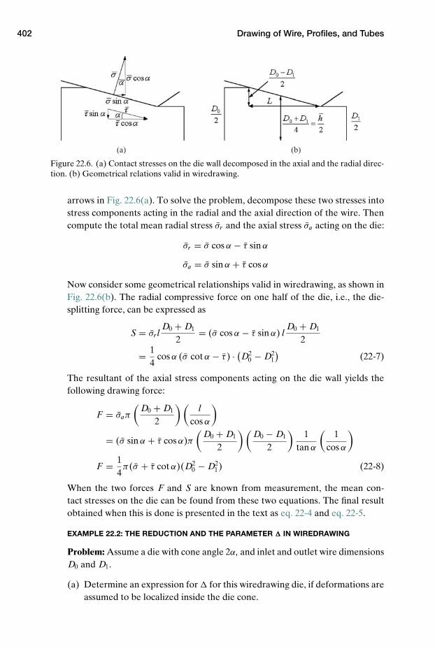
402 Drawing of Wire, Profiles, and Tubes
(a) (b)
Figure 22.6. (a) Contact stresses on the die wall decomposed in the axial and the radial direc-tion. (b) Geometrical relations valid in wiredrawing.
arrows in Fig. 22.6(a). To solve the problem, decompose these two stresses intostress components acting in the radial and the axial direction of the wire. Thencompute the total mean radial stress σr and the axial stress σa acting on the die:
σr = σ cos α − τ sin α
σa = σ sin α + τ cos α
Now consider some geometrical relationships valid in wiredrawing, as shown inFig. 22.6(b). The radial compressive force on one half of the die, i.e., the die-splitting force, can be expressed as
S = σr lD0 + D1
2= (σ cos α − τ sin α) l
D0 + D1
2
= 14
cos α (σ cot α − τ ) · (D2
0 − D21
)(22-7)
The resultant of the axial stress components acting on the die wall yields thefollowing drawing force:
F = σaπ
(D0 + D1
2
) (l
cos α
)
= (σ sin α + τ cos α)π(
D0 + D1
2
) (D0 − D1
2
)1
tan α
(1
cos α
)
F = 14π(σ + τ cot α)(D2
0 − D21) (22-8)
When the two forces F and S are known from measurement, the mean con-tact stresses on the die can be found from these two equations. The final resultobtained when this is done is presented in the text as eq. 22-4 and eq. 22-5.
EXAMPLE 22.2: THE REDUCTION AND THE PARAMETER � IN WIREDRAWING
Problem: Assume a die with cone angle 2α, and inlet and outlet wire dimensionsD0 and D1.
(a) Determine an expression for � for this wiredrawing die, if deformations areassumed to be localized inside the die cone.
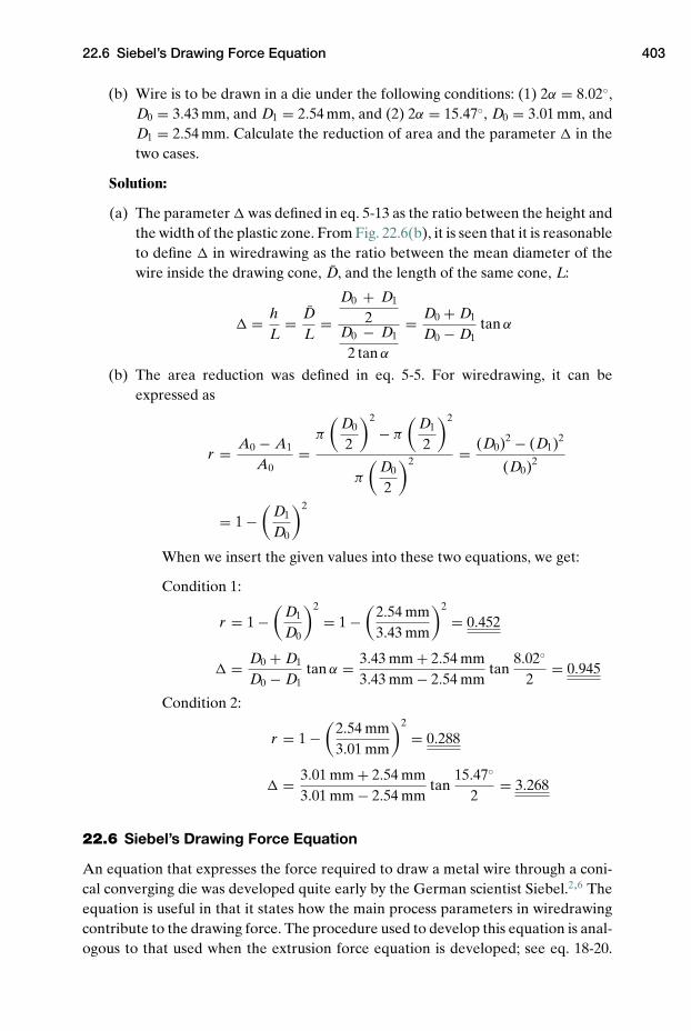
22.6 Siebel’s Drawing Force Equation 403
(b) Wire is to be drawn in a die under the following conditions: (1) 2α = 8.02◦,D0 = 3.43 mm, and D1 = 2.54 mm, and (2) 2α = 15.47◦, D0 = 3.01 mm, andD1 = 2.54 mm. Calculate the reduction of area and the parameter � in thetwo cases.
Solution:
(a) The parameter � was defined in eq. 5-13 as the ratio between the height andthe width of the plastic zone. From Fig. 22.6(b), it is seen that it is reasonableto define � in wiredrawing as the ratio between the mean diameter of thewire inside the drawing cone, D, and the length of the same cone, L:
� = hL
= DL
=D0 + D1
2D0 − D1
2 tan α
= D0 + D1
D0 − D1tan α
(b) The area reduction was defined in eq. 5-5. For wiredrawing, it can beexpressed as
r = A0 − A1
A0=
π
(D0
2
)2
− π
(D1
2
)2
π
(D0
2
)2 = (D0)2 − (D1)2
(D0)2
= 1 −(
D1
D0
)2
When we insert the given values into these two equations, we get:
Condition 1:
r = 1 −(
D1
D0
)2
= 1 −(
2.54 mm3.43 mm
)2
= 0.452
� = D0 + D1
D0 − D1tan α = 3.43 mm + 2.54 mm
3.43 mm − 2.54 mmtan
8.02◦
2= 0.945
Condition 2:
r = 1 −(
2.54 mm3.01 mm
)2
= 0.288
� = 3.01 mm + 2.54 mm3.01 mm − 2.54 mm
tan15.47◦
2= 3.268
22.6 Siebel’s Drawing Force Equation
An equation that expresses the force required to draw a metal wire through a coni-cal converging die was developed quite early by the German scientist Siebel.2,6 Theequation is useful in that it states how the main process parameters in wiredrawingcontribute to the drawing force. The procedure used to develop this equation is anal-ogous to that used when the extrusion force equation is developed; see eq. 18-20.
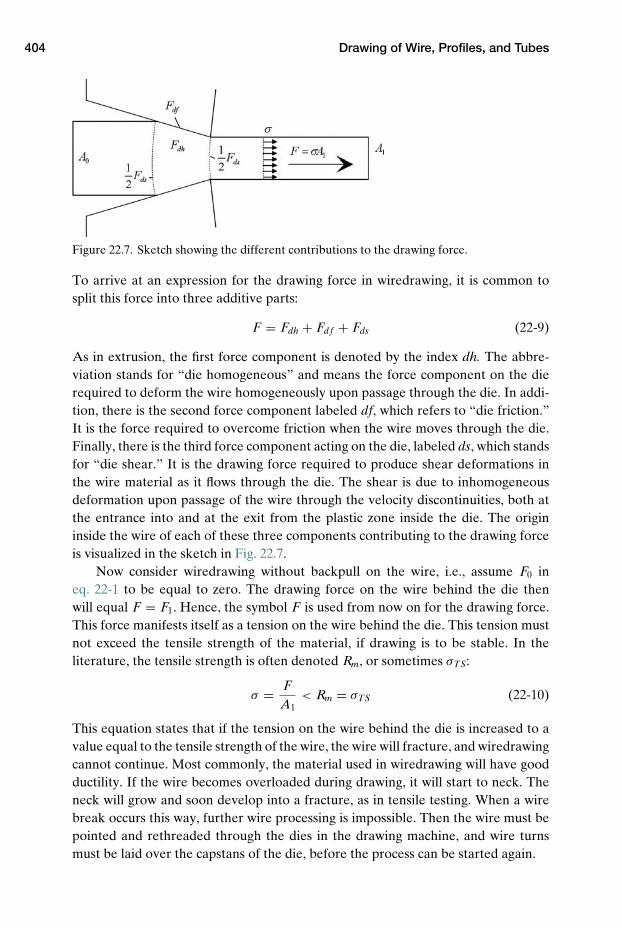
404 Drawing of Wire, Profiles, and Tubes
Figure 22.7. Sketch showing the different contributions to the drawing force.
To arrive at an expression for the drawing force in wiredrawing, it is common tosplit this force into three additive parts:
F = Fdh + Fdf + Fds (22-9)
As in extrusion, the first force component is denoted by the index dh. The abbre-viation stands for “die homogeneous” and means the force component on the dierequired to deform the wire homogeneously upon passage through the die. In addi-tion, there is the second force component labeled df, which refers to “die friction.”It is the force required to overcome friction when the wire moves through the die.Finally, there is the third force component acting on the die, labeled ds, which standsfor “die shear.” It is the drawing force required to produce shear deformations inthe wire material as it flows through the die. The shear is due to inhomogeneousdeformation upon passage of the wire through the velocity discontinuities, both atthe entrance into and at the exit from the plastic zone inside the die. The origininside the wire of each of these three components contributing to the drawing forceis visualized in the sketch in Fig. 22.7.
Now consider wiredrawing without backpull on the wire, i.e., assume F0 ineq. 22-1 to be equal to zero. The drawing force on the wire behind the die thenwill equal F = F1. Hence, the symbol F is used from now on for the drawing force.This force manifests itself as a tension on the wire behind the die. This tension mustnot exceed the tensile strength of the material, if drawing is to be stable. In theliterature, the tensile strength is often denoted Rm, or sometimes σTS:
σ = FA1
< Rm = σTS (22-10)
This equation states that if the tension on the wire behind the die is increased to avalue equal to the tensile strength of the wire, the wire will fracture, and wiredrawingcannot continue. Most commonly, the material used in wiredrawing will have goodductility. If the wire becomes overloaded during drawing, it will start to neck. Theneck will grow and soon develop into a fracture, as in tensile testing. When a wirebreak occurs this way, further wire processing is impossible. Then the wire must bepointed and rethreaded through the dies in the drawing machine, and wire turnsmust be laid over the capstans of the die, before the process can be started again.
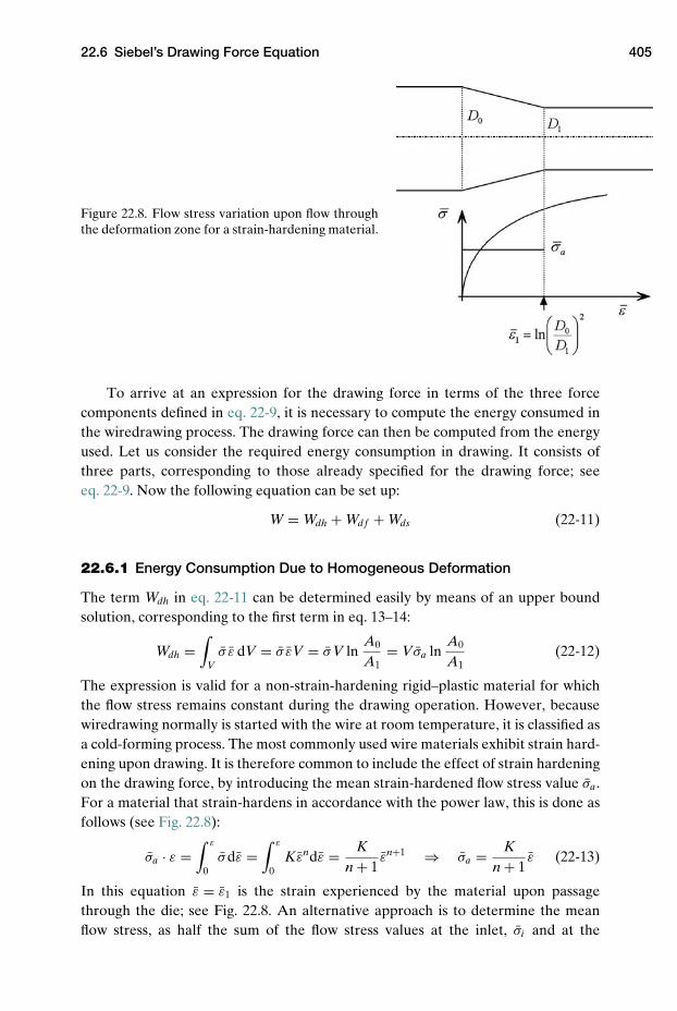
22.6 Siebel’s Drawing Force Equation 405
Figure 22.8. Flow stress variation upon flow throughthe deformation zone for a strain-hardening material.
To arrive at an expression for the drawing force in terms of the three forcecomponents defined in eq. 22-9, it is necessary to compute the energy consumed inthe wiredrawing process. The drawing force can then be computed from the energyused. Let us consider the required energy consumption in drawing. It consists ofthree parts, corresponding to those already specified for the drawing force; seeeq. 22-9. Now the following equation can be set up:
W = Wdh + Wdf + Wds (22-11)
22.6.1 Energy Consumption Due to Homogeneous Deformation
The term Wdh in eq. 22-11 can be determined easily by means of an upper boundsolution, corresponding to the first term in eq. 13–14:
Wdh =∫
Vσ ε dV = σ εV = σ V ln
A0
A1= Vσa ln
A0
A1(22-12)
The expression is valid for a non-strain-hardening rigid–plastic material for whichthe flow stress remains constant during the drawing operation. However, becausewiredrawing normally is started with the wire at room temperature, it is classified asa cold-forming process. The most commonly used wire materials exhibit strain hard-ening upon drawing. It is therefore common to include the effect of strain hardeningon the drawing force, by introducing the mean strain-hardened flow stress value σa .For a material that strain-hardens in accordance with the power law, this is done asfollows (see Fig. 22.8):
σa · ε =∫ ε
0σdε =
∫ ε
0Kεndε = K
n + 1εn+1 ⇒ σa = K
n + 1ε (22-13)
In this equation ε = ε1 is the strain experienced by the material upon passagethrough the die; see Fig. 22.8. An alternative approach is to determine the meanflow stress, as half the sum of the flow stress values at the inlet, σi and at the
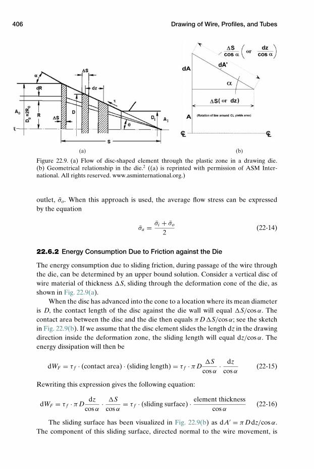
406 Drawing of Wire, Profiles, and Tubes
(a) (b)
Figure 22.9. (a) Flow of disc-shaped element through the plastic zone in a drawing die.(b) Geometrical relationship in the die.2 ((a) is reprinted with permission of ASM Inter-national. All rights reserved. www.asminternational.org.)
outlet, σo. When this approach is used, the average flow stress can be expressedby the equation
σa = σi + σo
2(22-14)
22.6.2 Energy Consumption Due to Friction against the Die
The energy consumption due to sliding friction, during passage of the wire throughthe die, can be determined by an upper bound solution. Consider a vertical disc ofwire material of thickness �S, sliding through the deformation cone of the die, asshown in Fig. 22.9(a).
When the disc has advanced into the cone to a location where its mean diameteris D, the contact length of the disc against the die wall will equal �S/cos α. Thecontact area between the disc and the die then equals π D�S/cos α; see the sketchin Fig. 22.9(b). If we assume that the disc element slides the length dz in the drawingdirection inside the deformation zone, the sliding length will equal dz/cos α. Theenergy dissipation will then be
dWF = τ f · (contact area) · (sliding length) = τ f · π D�S
cos α· dz
cos α(22-15)
Rewriting this expression gives the following equation:
dWF = τ f · π Ddz
cos α· �S
cos α= τ f · (sliding surface) · element thickness
cos α(22-16)
The sliding surface has been visualized in Fig. 22.9(b) as dA′ = π Ddz/cos α.The component of this sliding surface, directed normal to the wire movement, is
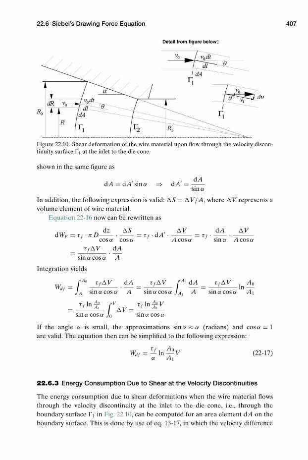
22.6 Siebel’s Drawing Force Equation 407
Figure 22.10. Shear deformation of the wire material upon flow through the velocity discon-tinuity surface �1 at the inlet to the die cone.
shown in the same figure as
dA = dA′ sin α ⇒ dA′ = dAsin α
In addition, the following expression is valid: �S = �V/A, where �V represents avolume element of wire material.
Equation 22-16 now can be rewritten as
dWF = τ f · π Ddz
cos α· �S
cos α= τ f · dA′ · �V
A cos α= τ f · dA
sin α· �V
A cos α
= τ f �Vsin α cos α
· dAA
Integration yields
Wdf =∫ A0
A1
τ f �Vsin α cos α
· dAA
= τ f �Vsin α cos α
∫ A0
A1
dAA
= τ f �Vsin α cos α
lnA0
A1
= τ f ln A0A1
sin α cos α
∫ V
0�V = τ f ln A0
A1V
sin α cos α
If the angle α is small, the approximations sin α ≈ α (radians) and cos α = 1are valid. The equation then can be simplified to the following expression:
Wdf = τ f
αln
A0
A1V (22-17)
22.6.3 Energy Consumption Due to Shear at the Velocity Discontinuities
The energy consumption due to shear deformations when the wire material flowsthrough the velocity discontinuity at the inlet to the die cone, i.e., through theboundary surface �1 in Fig. 22.10, can be computed for an area element dA on theboundary surface. This is done by use of eq. 13-17, in which the velocity difference
408 Drawing of Wire, Profiles, and Tubes
at the present velocity discontinuity is introduced (see Fig. 22.10):
WS =∫
Ak · |�v|dA ⇒ dWS = k · v0 sin θ dA dt (22-18)
This expression can further be developed into
dWS = k · v0 dt · sin θ dA = k · dlcos θ
· sin θ dA = k tan θ dl dA = k tan θ dV
(22-19)The quantities v0dt and dl represent the displacements of the wire into the defor-mation cone of the die, as shown in Fig. 22.10. Here dV represents the volume ofmaterial flowing through the area element dA during the time dt .
Assume the wire to be made of a von Mises material having the flow stress σ0 atthe inlet to the die. Then the following substitutions can be made in eq. 22–19:
k = σ0√3, dV = 2πR dR �S
In the latter expression, �S denotes the thickness of a disc of material at the inlet tothe die, as shown in Fig. 22.9(a). For small angles α and θ , the following approxima-tions can be made:
tan θ ≈ θ ≈ RS
, tan α ≈ α ≈ R0
S= D0
2S
In this expression, S denotes the whole length of the deformation cone; seeFig. 22.9(a). Equation 22-19 now can be transformed into the expression
�WS =∫ R0
0k tan θ dV = k
∫ R0
0
RS
2π RdR�S = k 2π�SS
∫ R0
0R2dR
= k 2π�SS
13
R30 = 2
3k
R0
Sπ R2
0 �S = 23
σ0√3α �V (22-20)
Here �V represents the material volume flowing through the deformation zone inthe time step dt . A total volume of wire material, V, flowing through the velocitydiscontinuity surface, yields the energy dissipation:
W�1S = �WS
V�V
= 23
σ0√3α �V · V
�V= 2
3σ0√
3αV (22-21)
A corresponding calculation of energy dissipation can be done for the same vol-ume of material when it flows through the velocity discontinuity line at the exit sideof the die, i.e., �2. This energy dissipation is equal to that during flow through thefirst discontinuity line, except for the effect of strain hardening of the material. Onits way through the plastic zone the material has strain-hardened up to a flow stressσ1. Hence, the total energy dissipation due to shearing when the material volume Vflows through the die will be
W�1+�2 = WS = 2
3√
3αV (σ0 + σ1) (22-22)
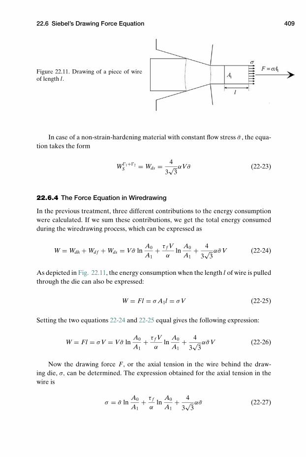
22.6 Siebel’s Drawing Force Equation 409
Figure 22.11. Drawing of a piece of wireof length l.
In case of a non-strain-hardening material with constant flow stress σ , the equa-tion takes the form
W�1+�2S = Wds = 4
3√
3αVσ (22-23)
22.6.4 The Force Equation in Wiredrawing
In the previous treatment, three different contributions to the energy consumptionwere calculated. If we sum these contributions, we get the total energy consumedduring the wiredrawing process, which can be expressed as
W = Wdh + Wdf + Wds = Vσ lnA0
A1+ τ f V
αln
A0
A1+ 4
3√
3ασ V (22-24)
As depicted in Fig. 22.11, the energy consumption when the length l of wire is pulledthrough the die can also be expressed:
W = Fl = σ A1l = σ V (22-25)
Setting the two equations 22-24 and 22-25 equal gives the following expression:
W = Fl = σ V = Vσ lnA0
A1+ τ f V
αln
A0
A1+ 4
3√
3ασ V (22-26)
Now the drawing force F , or the axial tension in the wire behind the draw-ing die, σ, can be determined. The expression obtained for the axial tension in thewire is
σ = σ lnA0
A1+ τ f
αln
A0
A1+ 4
3√
3ασ (22-27)
410 Drawing of Wire, Profiles, and Tubes
To arrive at a final equation for the drawing force (the wire tension in drawing), itis required to replace the friction stress term, τ f in eq. 22-27, by parameters easierto determine. When this is done, there are two options:
(1) Friction obeys the Tresca friction model, and the flow stress of the materialconforms to the von Mises flow criterion. In this case, the shear stress againstthe drawing die can be expressed by eq. 10-8, i.e., by
τ f = mσ√3
Substituting τ f in eq. 22-27 and then solving for the drawing force yields
F = σ A1 =(
σ lnA0
A1+ mσ√
3αln
A0
A1+ 4
3√
3ασ
)A1 (22-28)
(2) Friction obeys the Coulomb friction model, and the flow stress of the materialconforms to the Tresca flow criterion. Then the shear stress of the material canbe expressed as
k = σ
2
This modifies the term calculated in eq. 22-20. Let us also assume the wire mate-rial to be rigid–plastic without strain hardening, so the material has constantflow stress σ . Then eq. 22-27 instead can be expressed as
σ = σ lnA0
A1+ τ f
αln
A0
A1+ 2
3ασ (22-29)
In the case of Coulomb friction, the shear stress against the die wall can beexpressed by
τ f = µp = µσ
In this expression, σ is the normal stress transferred from the wire onto the diewall. For small angles α, this stress approximately equals the flow stress of thewire material:
τ f = µσ = µσ
The tension on the wire due to drawing, and thus the drawing force, then willbe given by
σ = σ lnA0
A1+ µσ
αln
A0
A1+ 2
3ασ (22-30)
and
F = A1σ = A1
(σ ln
A0
A1+ µσ
αln
A0
A1+ 2
3ασ
)(22-31)
The latter equation is commonly called Siebel’s drawing force equation, afterthe scientist who first developed it. If the wire material strain-hardens, the flowstress σ in the equation can be replaced by the mean flow stress of the materialin the drawing cone, expressed by eq. 22-13.
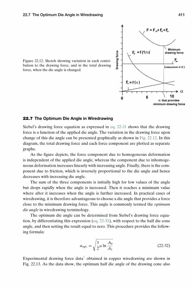
22.7 The Optimum Die Angle in Wiredrawing 411
Figure 22.12. Sketch showing variation in each contri-bution to the drawing force, and in the total drawingforce, when the die angle is changed.
22.7 The Optimum Die Angle in Wiredrawing
Siebel’s drawing force equation as expressed in eq. 22-31 shows that the drawingforce is a function of the applied die angle. The variation in the drawing force uponchange of this die angle can be presented graphically as shown in Fig. 22.12. In thisdiagram, the total drawing force and each force component are plotted as separategraphs.
As the figure depicts, the force component due to homogeneous deformationis independent of the applied die angle, whereas the component due to inhomoge-neous deformation increases linearly with increasing angle. Finally, there is the com-ponent due to friction, which is inversely proportional to the die angle and hencedecreases with increasing die angle.
The sum of the three components is initially high for low values of the anglebut drops rapidly when the angle is increased. Then it reaches a minimum valuewhere after it increases when the angle is further increased. In practical cases ofwiredrawing, it is therefore advantageous to choose a die angle that provides a forceclose to the minimum drawing force. This angle is commonly termed the optimumdie angle in wiredrawing terminology.
The optimum die angle can be determined from Siebel’s drawing force equa-tion, by differentiating this expression (eq. 22-31), with respect to the half die coneangle, and then setting the result equal to zero. This procedure provides the follow-ing formula:
αopt. =√
32µ ln
A0
A1(22-32)
Experimental drawing force data7 obtained in copper wiredrawing are shown inFig. 22.13. As the data show, the optimum half die angle of the drawing cone also
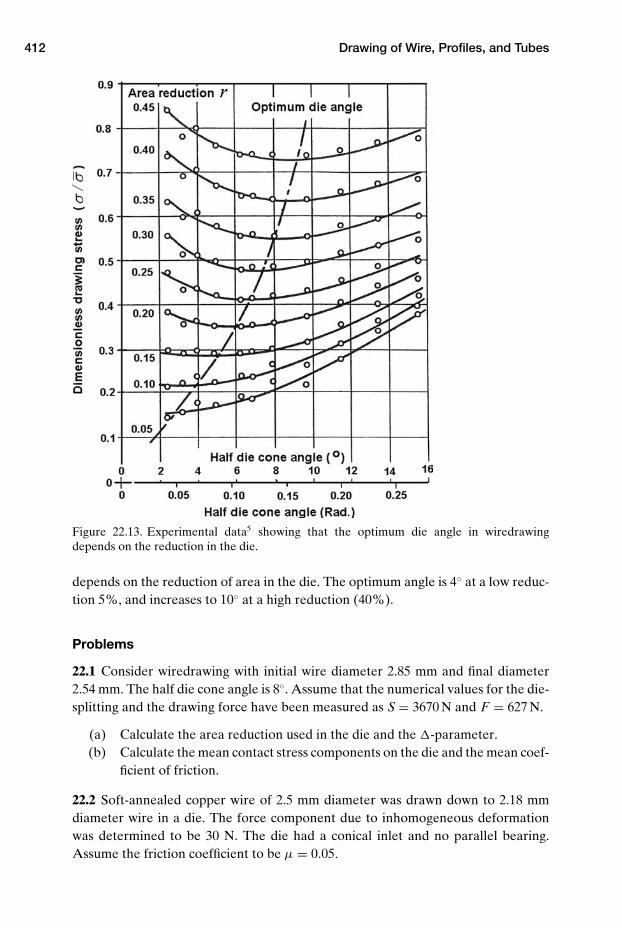
412 Drawing of Wire, Profiles, and Tubes
Figure 22.13. Experimental data5 showing that the optimum die angle in wiredrawingdepends on the reduction in the die.
depends on the reduction of area in the die. The optimum angle is 4◦ at a low reduc-tion 5%, and increases to 10◦ at a high reduction (40%).
Problems
22.1 Consider wiredrawing with initial wire diameter 2.85 mm and final diameter2.54 mm. The half die cone angle is 8◦. Assume that the numerical values for the die-splitting and the drawing force have been measured as S = 3670 N and F = 627 N.
(a) Calculate the area reduction used in the die and the �-parameter.(b) Calculate the mean contact stress components on the die and the mean coef-
ficient of friction.
22.2 Soft-annealed copper wire of 2.5 mm diameter was drawn down to 2.18 mmdiameter wire in a die. The force component due to inhomogeneous deformationwas determined to be 30 N. The die had a conical inlet and no parallel bearing.Assume the friction coefficient to be µ = 0.05.

Notes 413
(a) Find the required drawing force for the process by use of Siebel’s drawingforce equation. Assume the flow stress to be given by σ = 160ε0.3 MPa.
(b) Discuss the different components that contribute to the total drawing force.(c) Determine the optimum die cone angle for this wiredrawing operation.
NOTES
1. Dieter, G.: “Mechanical Metallurgy,” McGraw-Hill Book Company, 1987, p. 636.2. Altan, T., Oh, S.-I., and Gegel, H. L.: “Metal Forming, Fundamentals and Applications,”
ASM Int., 1983, pp. 277–293.3. MacLellan, G. D. S.: “A critical survey of wire-drawing theory,” J. Iron and Steel Insti-
tuta, 1948, pp. 347–356.4. MacLellan, G. D. S.: “Some friction effects in wiredrawing,” J. Institute of Metals,
Vol. 81, 1952–53, pp. 1–13.5. Wistreich J. G.: “Investigation of the mechanics of wire drawing,” Proc. Institute of
Mechanical Engineers, 169, 1955, pp. 654–665.6. Lange, Kurt (Ed.): “Handbook of Metal Forming,” McGraw-Hill, p. 13.20.7. Wistreich, J. G.: “The fundamentals of wiredrawing,” Metallurgical Rev., Vol. 3, 1958,
pp. 97–142.
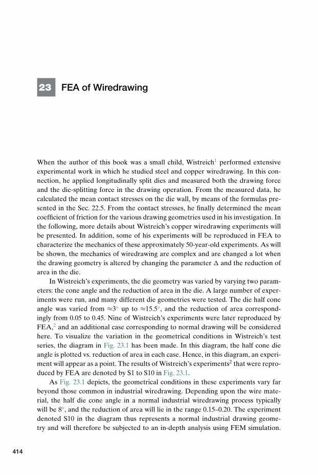
23 FEA of Wiredrawing
When the author of this book was a small child, Wistreich1 performed extensiveexperimental work in which he studied steel and copper wiredrawing. In this con-nection, he applied longitudinally split dies and measured both the drawing forceand the die-splitting force in the drawing operation. From the measured data, hecalculated the mean contact stresses on the die wall, by means of the formulas pre-sented in the Sec. 22.5. From the contact stresses, he finally determined the meancoefficient of friction for the various drawing geometries used in his investigation. Inthe following, more details about Wistreich’s copper wiredrawing experiments willbe presented. In addition, some of his experiments will be reproduced in FEA tocharacterize the mechanics of these approximately 50-year-old experiments. As willbe shown, the mechanics of wiredrawing are complex and are changed a lot whenthe drawing geometry is altered by changing the parameter � and the reduction ofarea in the die.
In Wistreich’s experiments, the die geometry was varied by varying two param-eters: the cone angle and the reduction of area in the die. A large number of exper-iments were run, and many different die geometries were tested. The die half coneangle was varied from ≈3◦ up to ≈15.5◦, and the reduction of area correspond-ingly from 0.05 to 0.45. Nine of Wistreich’s experiments were later reproduced byFEA,2 and an additional case corresponding to normal drawing will be consideredhere. To visualize the variation in the geometrical conditions in Wistreich’s testseries, the diagram in Fig. 23.1 has been made. In this diagram, the half cone dieangle is plotted vs. reduction of area in each case. Hence, in this diagram, an experi-ment will appear as a point. The results of Wistreich’s experiments2 that were repro-duced by FEA are denoted by S1 to S10 in Fig. 23.1.
As Fig. 23.1 depicts, the geometrical conditions in these experiments vary farbeyond those common in industrial wiredrawing. Depending upon the wire mate-rial, the half die cone angle in a normal industrial wiredrawing process typicallywill be 8◦, and the reduction of area will lie in the range 0.15–0.20. The experimentdenoted S10 in the diagram thus represents a normal industrial drawing geome-try and will therefore be subjected to an in-depth analysis using FEM simulation.
414
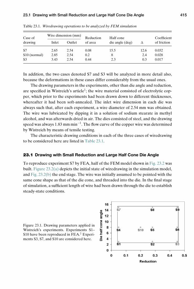
23.1 Drawing with Small Reduction and Large Half Cone Die Angle 415
Table 23.1. Wiredrawing operations to be analyzed by FEM simulation
Wire dimension (mm)Case of Reduction Half cone Coefficientdrawing Inlet Outlet of area die angle (deg) � of friction
S7 2.65 2.54 0.08 15.5 12.6 0.032S10 (normal) 2.85 2.54 0.2 8 2.4 0.028S3 3.43 2.54 0.44 2.3 0.3 0.017
In addition, the two cases denoted S7 and S3 will be analyzed in more detail also,because the deformations in these cases differ considerably from the usual ones.
The drawing parameters in the experiments, other than die angle and reduction,are specified in Wistreich’s article1; the wire material consisted of electrolytic cop-per, which prior to the experiments had been drawn down to different thicknesses,whereafter it had been soft-annealed. The inlet wire dimension in each die wasalways such that, after each experiment, a wire diameter of 2.54 mm was obtained.The wire was lubricated by dipping it in a solution of sodium stearate in methylalcohol, and was afterwards dried in air. The dies consisted of steel, and the drawingspeed was always 1.83 mm min−1. The flow curve of the copper wire was determinedby Wistreich by means of tensile testing.
The characteristic drawing conditions in each of the three cases of wiredrawingto be considered here are listed in Table 23.1.
23.1 Drawing with Small Reduction and Large Half Cone Die Angle
To reproduce experiment S7 by FEA, half of the FEM model shown in Fig. 23.2 wasbuilt. Figure 23.2(a) depicts the initial state of wiredrawing in the simulation model,and Fig. 23.2(b) the end stage. The wire was initially assumed to be pointed with thesame cone shape as that of the die cone, and threaded into the die. In the final stageof simulation, a sufficient length of wire had been drawn through the die to establishsteady-state conditions.
Figure 23.1. Drawing parameters applied inWistreich’s experiments. Experiments S1–S10 have been reproduced in FEA.2 Experi-ments S3, S7, and S10 are considered here.
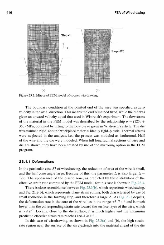
416 FEA of Wiredrawing
(a) (b)
Step -526
Step -1
Y
X
Figure 23.2. Mirrored FEM model of copper wiredrawing.
The boundary condition at the pointed end of the wire was specified as zerovelocity in the axial direction. This means the end remained fixed, while the die wasgiven an upward velocity equal that used in Wistreich’s experiment. The flow stressof the material in the FEM model was described by the relationship σ = (125ε +360) MPa, obtained by fitting to the flow curve given in Wistreich’s article. The diewas assumed rigid, and the workpiece material ideally rigid–plastic. Thermal effectswere neglected in the analysis, i.e., the process was modeled as isothermal. Halfof the wire and the die were modeled. When full longitudinal sections of wire anddie are shown, they have been created by use of the mirroring option in the FEMprogram.
23.1.1 Deformations
In the particular case S7 of wiredrawing, the reduction of area of the wire is small,and the half cone angle large. Because of this, the parameter � is also large: � =12.6. The appearance of the plastic zone, as predicted by the distribution of theeffective strain rate computed by the FEM model, for this case is shown in Fig. 23.3.
There is close resemblance between Fig. 23.3(b), which represents wiredrawing,and Fig. 21.2(b), which represents plane strain rolling, both characterized by use ofsmall reduction in the forming step, and therefore a large �. As Fig. 23.3 depicts,the deformation rate in the core of the wire lies in the range ≈5–7 s−1 and is muchlower than the corresponding strain rate toward the surface layer of the wire, whichis >9 s−1. Locally, close to the die surface, it is much higher and the maximumpredicted effective strain rate reaches 168–198 s−1.
In this case of wiredrawing, as shown in Fig. 23.3(a) and (b), the high-strain-rate region near the surface of the wire extends into the material ahead of the die
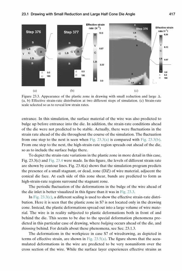
23.1 Drawing with Small Reduction and Large Half Cone Die Angle 417
(a) (b) (c)
Figure 23.3. Appearance of the plastic zone in drawing with small reduction and large �.(a, b) Effective strain-rate distribution at two different steps of simulation. (c) Strain-ratescale selected so as to reveal low strain rates.
entrance. In this simulation, the surface material of the wire was also predicted tobulge up before entrance into the die. In addition, the strain-rate conditions aheadof the die were not predicted to be stable. Actually, there were fluctuations in thestrain rate ahead of the die throughout the course of the simulation. The fluctuationfrom one step to the next is seen when Fig. 23.3(a) is compared with Fig. 23.3(b).From one step to the next, the high-strain-rate region spreads out ahead of the die,so as to include the surface bulge there.
To depict the strain-rate variations in the plastic zone in more detail in this case,Fig. 23.3(c) and Fig. 23.4 were made. In this figure, the levels of different strain rateare shown by contour lines. Fig. 23.4(a) shows that the simulation program predictsthe presence of a small stagnant, or dead, zone (DZ) of wire material, adjacent theconical die face. At each side of this zone shear, bands are predicted to form ashigh-strain-rate regions surround the stagnant zone.
The periodic fluctuation of the deformations in the bulge of the wire ahead ofthe die inlet is better visualized in this figure than it was in Fig. 23.3.
In Fig. 23.3(c), a different scaling is used to show the effective strain-rate distri-bution. Here it is seen that the plastic zone in S7 is not located only in the drawingcone. Instead, the plastic deformations spread out into a large volume of wire mate-rial. The wire is in reality subjected to plastic deformations both in front of andbehind the die. This seems to be due to the special deformation phenomena pre-dicted in this particular case of drawing, where bulging occurs ahead of the die, andthinning behind. For details about these phenomena, see Sec. 23.1.3.
The deformations in the workpiece in case S7 of wiredrawing, as depicted interms of effective strain, are shown in Fig. 23.5(a). The figure shows that the accu-mulated deformations in the wire are predicted to be very nonuniform over thecross section of the wire. While the surface layer experiences effective strains as
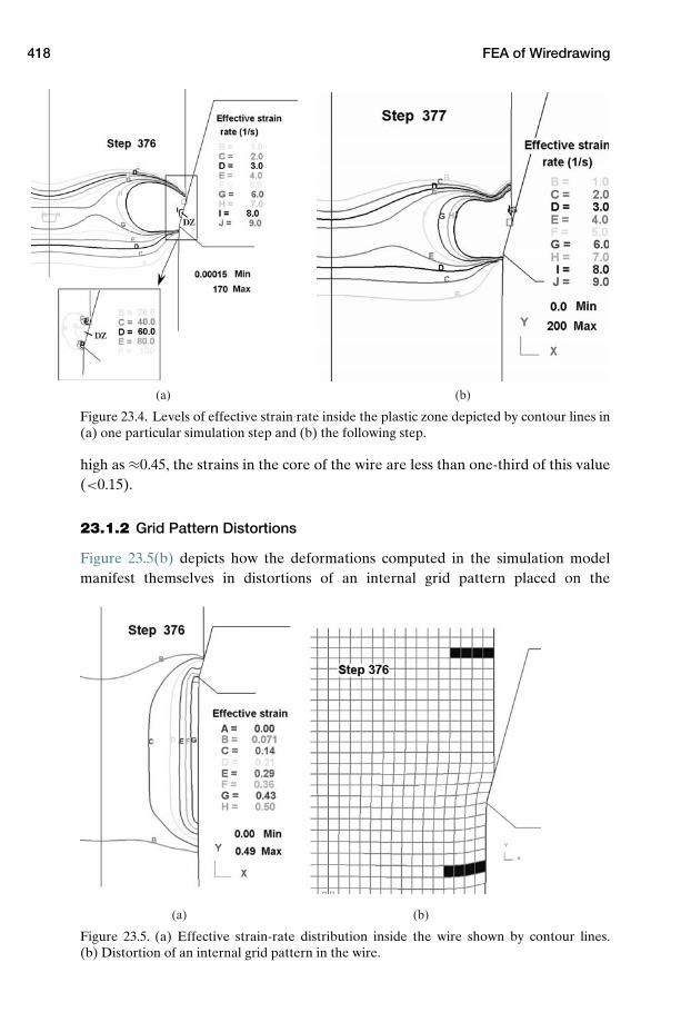
418 FEA of Wiredrawing
(a) (b)
Figure 23.4. Levels of effective strain rate inside the plastic zone depicted by contour lines in(a) one particular simulation step and (b) the following step.
high as ≈0.45, the strains in the core of the wire are less than one-third of this value(<0.15).
23.1.2 Grid Pattern Distortions
Figure 23.5(b) depicts how the deformations computed in the simulation modelmanifest themselves in distortions of an internal grid pattern placed on the
(a) (b)
Figure 23.5. (a) Effective strain-rate distribution inside the wire shown by contour lines.(b) Distortion of an internal grid pattern in the wire.
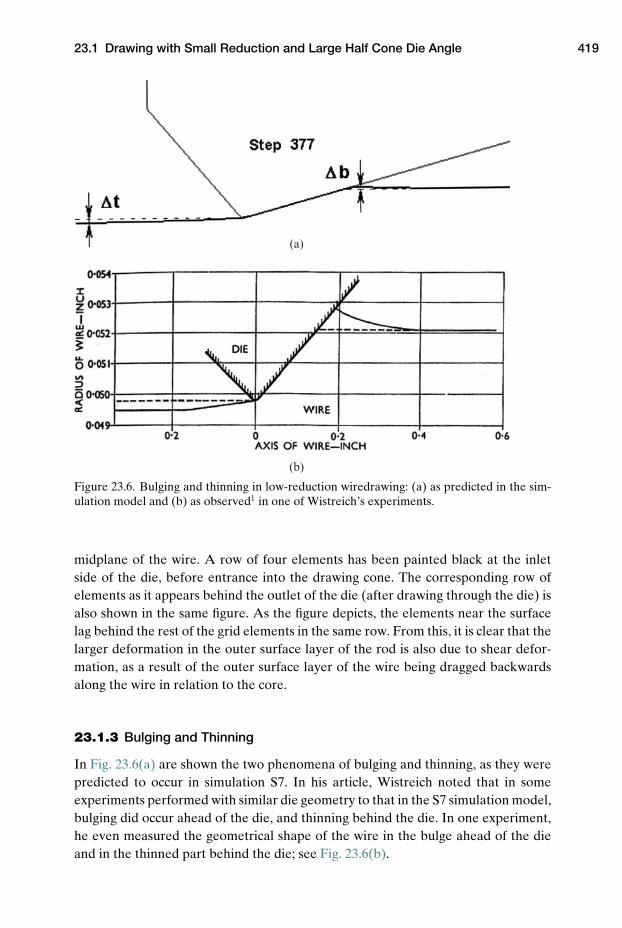
23.1 Drawing with Small Reduction and Large Half Cone Die Angle 419
(a)
(b)
Figure 23.6. Bulging and thinning in low-reduction wiredrawing: (a) as predicted in the sim-ulation model and (b) as observed1 in one of Wistreich’s experiments.
midplane of the wire. A row of four elements has been painted black at the inletside of the die, before entrance into the drawing cone. The corresponding row ofelements as it appears behind the outlet of the die (after drawing through the die) isalso shown in the same figure. As the figure depicts, the elements near the surfacelag behind the rest of the grid elements in the same row. From this, it is clear that thelarger deformation in the outer surface layer of the rod is also due to shear defor-mation, as a result of the outer surface layer of the wire being dragged backwardsalong the wire in relation to the core.
23.1.3 Bulging and Thinning
In Fig. 23.6(a) are shown the two phenomena of bulging and thinning, as they werepredicted to occur in simulation S7. In his article, Wistreich noted that in someexperiments performed with similar die geometry to that in the S7 simulation model,bulging did occur ahead of the die, and thinning behind the die. In one experiment,he even measured the geometrical shape of the wire in the bulge ahead of the dieand in the thinned part behind the die; see Fig. 23.6(b).
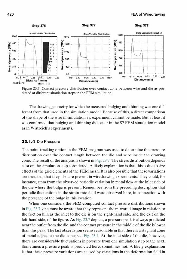
420 FEA of Wiredrawing
Figure 23.7. Contact pressure distribution over contact zone between wire and die as pre-dicted at different simulation steps in the FEM simulation.
The drawing geometry for which he measured bulging and thinning was one dif-ferent from that used in the simulation model. Because of this, a direct comparisonof the shape of the wire in simulation vs. experiment cannot be made. But at least itwas confirmed that bulging and thinning did occur in the S7 FEM simulation modelas in Wistreich’s experiments.
23.1.4 Die Pressure
The point-tracking option in the FEM program was used to determine the pressuredistribution over the contact length between the die and wire inside the drawingcone. The result of the analysis is shown in Fig. 23.7. The stress distribution dependsa lot on the simulation step considered. A likely explanation is that this is due to sizeeffects of the grid elements of the FEM mesh. It is also possible that these variationsare true, i.e., that they also are present in wiredrawing experiments. They could, forinstance, stem from the observed periodic variation in metal flow at the inlet side ofthe die where the bulge is present. Remember from the preceding description thatperiodic fluctuations in the strain-rate field were observed here, in connection withthe presence of the bulge in this location.
When one considers the FEM-computed contact pressure distributions shownin Fig. 23.7, one must be aware that they represent the mirrored image in relation tothe friction hill, as the inlet to the die is on the right-hand side, and the exit on theleft-hand side, of the figure. As Fig. 23.7 depicts, a pressure peak is always predictednear the outlet from the die, and the contact pressure in the middle of the die is lowerthan this peak. The last observation seems reasonable in that there is a stagnant zoneof metal adjacent the die cone; see Fig. 23.4. At the inlet side of the die, however,there are considerable fluctuations in pressure from one simulation step to the next.Sometimes a pressure peak is predicted here, sometimes not. A likely explanationis that these pressure variations are caused by variations in the deformation field in

23.1 Drawing with Small Reduction and Large Half Cone Die Angle 421
Figure 23.8. Distribution of the damage parameter in thelongitudinal section of the wire, shown by grayscale.
the bulge ahead of the die, which in turn generate stepwise fluctuations in the strainrate inside the wire, as already explained in connection with Fig. 23.3 and Fig. 23.4.
23.1.5 Damage Parameter and the Formation of Chevron Cracks
In Fig. 23.8 is shown the FEM-predicted value of the damage parameter, com-puted according to the Cockcroft–Latham criterion. The figure shows this param-eter in terms of the distribution of the parameter along the axial midsection of thedrawn wire. A similar representation of the simulated damage parameter is shown inFig. 23.9, but with a different scaling to visualize predicted variations in the damageparameter at the center of the wire. Here center burst or chevron cracks are likelyto be formed3 when unfavorable geometrical conditions are used in the drawingprocess, as in our analysis.
The highest level of the damage parameter is seen to be along the axis of thewire. In Fig. 23.9, the wire and the die have been oriented horizontally, in contrastto the vertical picture shown in Fig. 23.8. The simulation that was run in this casewas identical to the previously mentioned simulation model of case S7, except thatnow a longer length of wire was pulled through the die.
As shown in Fig. 23.9(a), the FEM program predicts periodic variations in thedamage factor along the axis of the wire. Because of this, voids can in principle beinitiated periodically along this axis, at each maximum of the damage factor. Thiscould explain why chevron cracks tend to appear periodically, with approximatelyconstant distance between them, when wire is drawn through dies with small reduc-tion and large die cone angle.
An attempt was made to find what could cause the variations in the damagefactor. It seemed natural to check the simulated effective strain, for this parametercontributes to the damage factor. It was found that this parameter varied in thesame manner along the axis of the wire as the damage parameter, i.e., with peakvalues occurring at fixed intervals; see Fig. 23.9(b). Further investigations into this
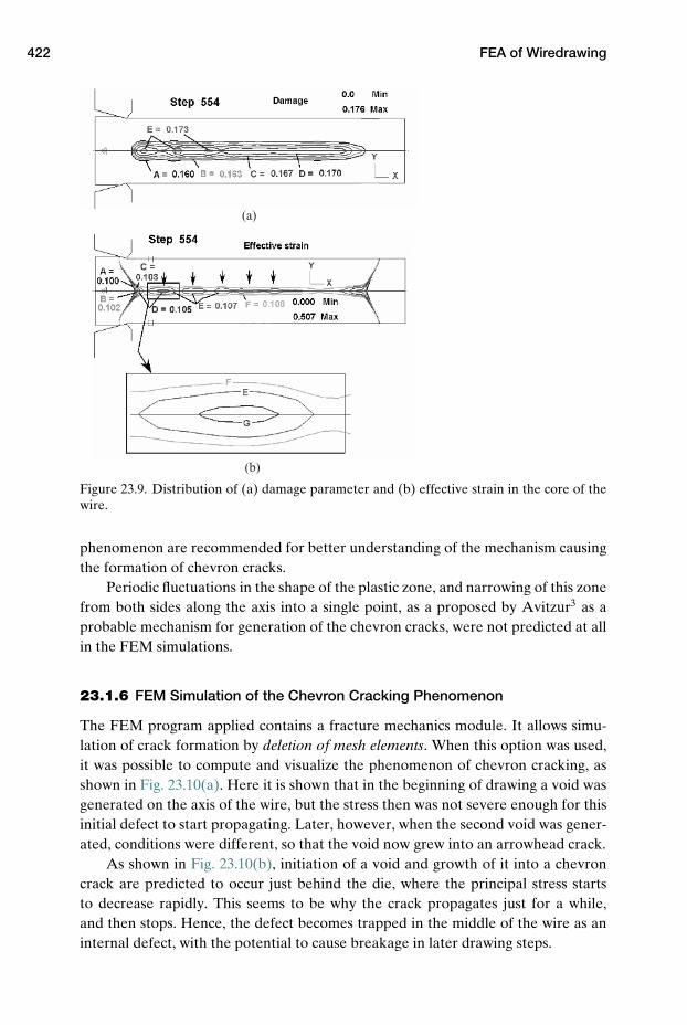
422 FEA of Wiredrawing
(a)
(b)
Figure 23.9. Distribution of (a) damage parameter and (b) effective strain in the core of thewire.
phenomenon are recommended for better understanding of the mechanism causingthe formation of chevron cracks.
Periodic fluctuations in the shape of the plastic zone, and narrowing of this zonefrom both sides along the axis into a single point, as a proposed by Avitzur3 as aprobable mechanism for generation of the chevron cracks, were not predicted at allin the FEM simulations.
23.1.6 FEM Simulation of the Chevron Cracking Phenomenon
The FEM program applied contains a fracture mechanics module. It allows simu-lation of crack formation by deletion of mesh elements. When this option was used,it was possible to compute and visualize the phenomenon of chevron cracking, asshown in Fig. 23.10(a). Here it is shown that in the beginning of drawing a void wasgenerated on the axis of the wire, but the stress then was not severe enough for thisinitial defect to start propagating. Later, however, when the second void was gener-ated, conditions were different, so that the void now grew into an arrowhead crack.
As shown in Fig. 23.10(b), initiation of a void and growth of it into a chevroncrack are predicted to occur just behind the die, where the principal stress startsto decrease rapidly. This seems to be why the crack propagates just for a while,and then stops. Hence, the defect becomes trapped in the middle of the wire as aninternal defect, with the potential to cause breakage in later drawing steps.
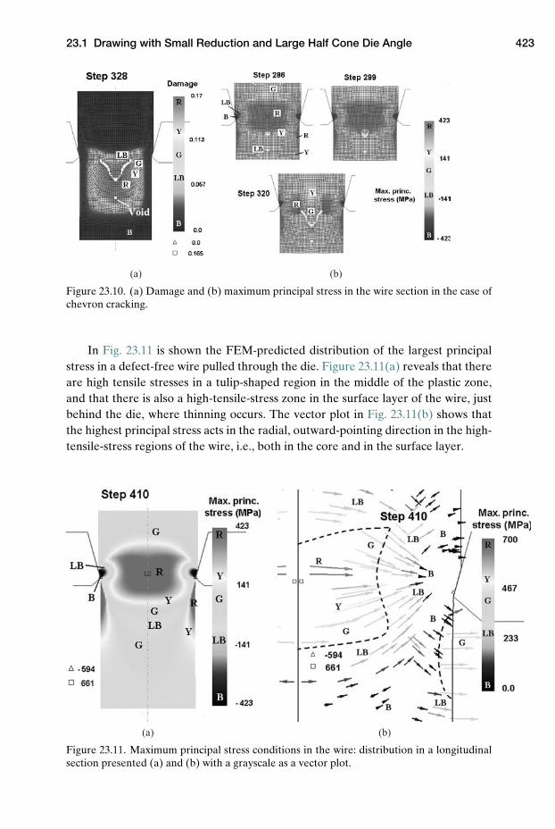
23.1 Drawing with Small Reduction and Large Half Cone Die Angle 423
(a) (b)
Figure 23.10. (a) Damage and (b) maximum principal stress in the wire section in the case ofchevron cracking.
In Fig. 23.11 is shown the FEM-predicted distribution of the largest principalstress in a defect-free wire pulled through the die. Figure 23.11(a) reveals that thereare high tensile stresses in a tulip-shaped region in the middle of the plastic zone,and that there is also a high-tensile-stress zone in the surface layer of the wire, justbehind the die, where thinning occurs. The vector plot in Fig. 23.11(b) shows thatthe highest principal stress acts in the radial, outward-pointing direction in the high-tensile-stress regions of the wire, i.e., both in the core and in the surface layer.
(a) (b)
Figure 23.11. Maximum principal stress conditions in the wire: distribution in a longitudinalsection presented (a) and (b) with a grayscale as a vector plot.
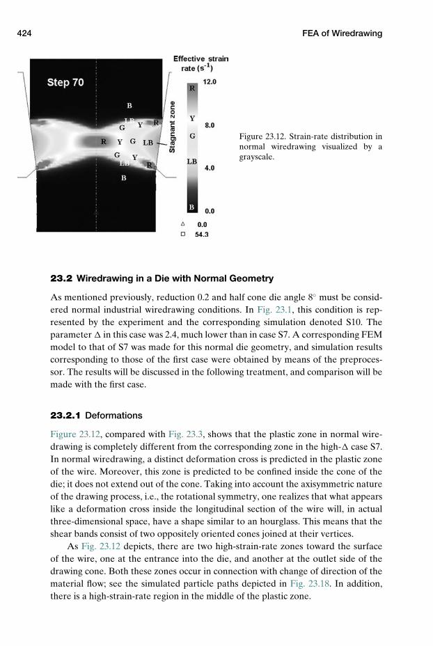
424 FEA of Wiredrawing
Figure 23.12. Strain-rate distribution innormal wiredrawing visualized by agrayscale.
23.2 Wiredrawing in a Die with Normal Geometry
As mentioned previously, reduction 0.2 and half cone die angle 8◦ must be consid-ered normal industrial wiredrawing conditions. In Fig. 23.1, this condition is rep-resented by the experiment and the corresponding simulation denoted S10. Theparameter � in this case was 2.4, much lower than in case S7. A corresponding FEMmodel to that of S7 was made for this normal die geometry, and simulation resultscorresponding to those of the first case were obtained by means of the preproces-sor. The results will be discussed in the following treatment, and comparison will bemade with the first case.
23.2.1 Deformations
Figure 23.12, compared with Fig. 23.3, shows that the plastic zone in normal wire-drawing is completely different from the corresponding zone in the high-� case S7.In normal wiredrawing, a distinct deformation cross is predicted in the plastic zoneof the wire. Moreover, this zone is predicted to be confined inside the cone of thedie; it does not extend out of the cone. Taking into account the axisymmetric natureof the drawing process, i.e., the rotational symmetry, one realizes that what appearslike a deformation cross inside the longitudinal section of the wire will, in actualthree-dimensional space, have a shape similar to an hourglass. This means that theshear bands consist of two oppositely oriented cones joined at their vertices.
As Fig. 23.12 depicts, there are two high-strain-rate zones toward the surfaceof the wire, one at the entrance into the die, and another at the outlet side of thedrawing cone. Both these zones occur in connection with change of direction of thematerial flow; see the simulated particle paths depicted in Fig. 23.18. In addition,there is a high-strain-rate region in the middle of the plastic zone.
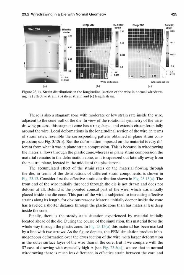
23.2 Wiredrawing in a Die with Normal Geometry 425
(a) (b) (c)
Figure 23.13. Strain distributions in the longitudinal section of the wire in normal wiredraw-ing: (a) effective strain, (b) shear strain, and (c) length strain.
There is also a stagnant zone with moderate or low strain rate inside the wire,adjacent to the cone wall of the die. In view of the rotational symmetry of the wire-drawing process, this stagnant zone has a ring shape, and extends circumferentiallyaround the wire. Local deformations in the longitudinal section of the wire, in termsof strain rates, resemble the corresponding pattern obtained in plane strain com-pression; see Fig. 3.12(b). But the deformation imposed on the material is very dif-ferent from what it was in plane strain compression. This is because in wiredrawingthe material flows through the plastic zone,whereas in plane strain compression thematerial remains in the deformation zone, as it is squeezed out laterally away fromthe neutral plane, located in the middle of the plastic zone.
The accumulated effect of the strain rates on the material flowing throughthe die, in terms of the distributions of different strain components, is shown inFig. 23.13. Consider first the effective strain distribution shown in Fig. 23.13(a). Thefront end of the wire initially threaded through the die is not drawn and does notdeform at all. Behind is the pointed conical part of the wire, which was initiallyplaced inside the die cone. This part of the wire is subjected to increasing effectivestrains along its length, for obvious reasons: Material initially deeper inside the conehas traveled a shorter distance through the plastic zone than has material less deepinside the cone.
Finally, there is the steady-state situation experienced by material initiallylocated ahead of the die. During the course of the simulation, this material flows thewhole way through the plastic zone. In Fig. 23.13(a) this material has been markedby a line with two arrows. As the figure depicts, the FEM simulation predicts inho-mogeneous deformation over the cross section of the wire, with larger deformationin the outer surface layer of the wire than in the core. But if we compare with theS7 case of drawing with especially high � [see Fig. 23.5(a)], we see that in normalwiredrawing there is much less difference in effective strain between the core and
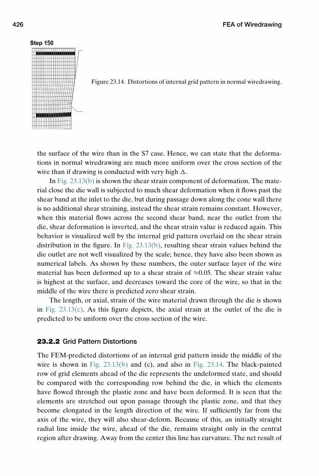
426 FEA of Wiredrawing
Figure 23.14. Distortions of internal grid pattern in normal wiredrawing.
the surface of the wire than in the S7 case. Hence, we can state that the deforma-tions in normal wiredrawing are much more uniform over the cross section of thewire than if drawing is conducted with very high �.
In Fig. 23.13(b) is shown the shear strain component of deformation. The mate-rial close the die wall is subjected to much shear deformation when it flows past theshear band at the inlet to the die, but during passage down along the cone wall thereis no additional shear straining, instead the shear strain remains constant. However,when this material flows across the second shear band, near the outlet from thedie, shear deformation is inverted, and the shear strain value is reduced again. Thisbehavior is visualized well by the internal grid pattern overlaid on the shear straindistribution in the figure. In Fig. 23.13(b), resulting shear strain values behind thedie outlet are not well visualized by the scale; hence, they have also been shown asnumerical labels. As shown by these numbers, the outer surface layer of the wirematerial has been deformed up to a shear strain of ≈0.05. The shear strain valueis highest at the surface, and decreases toward the core of the wire, so that in themiddle of the wire there is predicted zero shear strain.
The length, or axial, strain of the wire material drawn through the die is shownin Fig. 23.13(c). As this figure depicts, the axial strain at the outlet of the die ispredicted to be uniform over the cross section of the wire.
23.2.2 Grid Pattern Distortions
The FEM-predicted distortions of an internal grid pattern inside the middle of thewire is shown in Fig. 23.13(b) and (c), and also in Fig. 23.14. The black-paintedrow of grid elements ahead of the die represents the undeformed state, and shouldbe compared with the corresponding row behind the die, in which the elementshave flowed through the plastic zone and have been deformed. It is seen that theelements are stretched out upon passage through the plastic zone, and that theybecome elongated in the length direction of the wire. If sufficiently far from theaxis of the wire, they will also shear-deform. Because of this, an initially straightradial line inside the wire, ahead of the die, remains straight only in the centralregion after drawing. Away from the center this line has curvature. The net result of
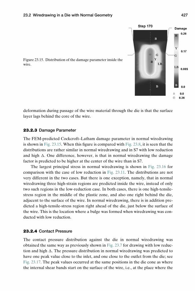
23.2 Wiredrawing in a Die with Normal Geometry 427
Figure 23.15. Distribution of the damage parameter inside thewire.
deformation during passage of the wire material through the die is that the surfacelayer lags behind the core of the wire.
23.2.3 Damage Parameter
The FEM-predicted Cockcroft–Latham damage parameter in normal wiredrawingis shown in Fig. 23.15. When this figure is compared with Fig. 23.8, it is seen that thedistributions are rather similar in normal wiredrawing and in S7 with low reductionand high �. One difference, however, is that in normal wiredrawing the damagefactor is predicted to be higher at the center of the wire than in S7.
The largest principal stress in normal wiredrawing is shown in Fig. 23.16 forcomparison with the case of low reduction in Fig. 23.11. The distributions are notvery different in the two cases. But there is one exception, namely, that in normalwiredrawing three high-strain regions are predicted inside the wire, instead of onlytwo such regions in the low-reduction case. In both cases, there is one high-tensile-stress region in the middle of the plastic zone, and also one right behind the die,adjacent to the surface of the wire. In normal wiredrawing, there is in addition pre-dicted a high-tensile-stress region right ahead of the die, just below the surface ofthe wire. This is the location where a bulge was formed when wiredrawing was con-ducted with low reduction.
23.2.4 Contact Pressure
The contact pressure distribution against the die in normal wiredrawing wasobtained the same way as previously shown in Fig. 23.7 for drawing with low reduc-tion and high �. The pressure distribution in normal wiredrawing was predicted tohave one peak value close to the inlet, and one close to the outlet from the die; seeFig. 23.17. The peak values occurred at the same positions in the die cone as wherethe internal shear bands start on the surface of the wire, i.e., at the place where the
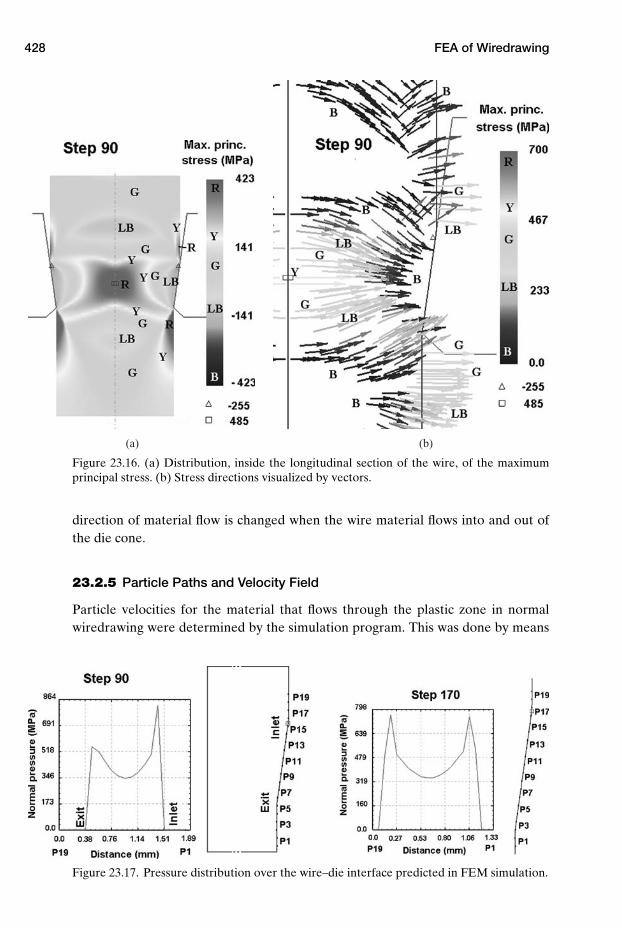
428 FEA of Wiredrawing
(a) (b)
Figure 23.16. (a) Distribution, inside the longitudinal section of the wire, of the maximumprincipal stress. (b) Stress directions visualized by vectors.
direction of material flow is changed when the wire material flows into and out ofthe die cone.
23.2.5 Particle Paths and Velocity Field
Particle velocities for the material that flows through the plastic zone in normalwiredrawing were determined by the simulation program. This was done by means
Figure 23.17. Pressure distribution over the wire–die interface predicted in FEM simulation.
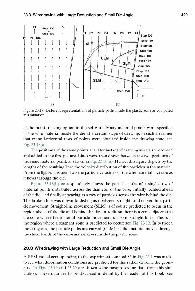
23.3 Wiredrawing with Large Reduction and Small Die Angle 429
(a) (b)
Figure 23.18. Different representations of particle paths inside the plastic zone as computedin simulation.
of the point-tracking option in the software. Many material points were specifiedin the wire material inside the die at a certain stage of drawing, in such a mannerthat many horizontal rows of points were obtained inside the drawing cone; seeFig. 23.18(a).
The positions of the same points at a later instant of drawing were also recordedand added to the first picture. Lines were then drawn between the two positions ofthe same material point, as shown in Fig. 23.18(a). Hence, this figure depicts by thelengths of the resulting lines the velocity distribution of the particles in the material.From the figure, it is seen how the particle velocities of the wire material increase asit flows through the die.
Figure 23.18(b) correspondingly shows the particle paths of a single row ofmaterial points distributed across the diameter of the wire, initially located aheadof the die, and finally appearing as a row of particles across the wire behind the die.The broken line was drawn to distinguish between straight- and curved-line parti-cle movement. Straight-line movement (SLM) is of course predicted to occur in theregion ahead of the die and behind the die. In addition there is a zone adjacent thedie cone where the material particle movement is also in straight lines. This is inthe region where a stagnant zone is predicted to occur; see Fig. 23.12. In betweenthese regions, the particle paths are curved (CLM), as the material moves throughthe shear bands of the deformation cross inside the plastic zone.
23.3 Wiredrawing with Large Reduction and Small Die Angle
A FEM model corresponding to the experiment denoted S3 in Fig. 23.1 was made,to see what deformation conditions are predicted for this rather extreme die geom-etry. In Figs. 23.19 and 23.20 are shown some postprocessing data from this sim-ulation. These data are to be discussed in detail by the reader of this book; see
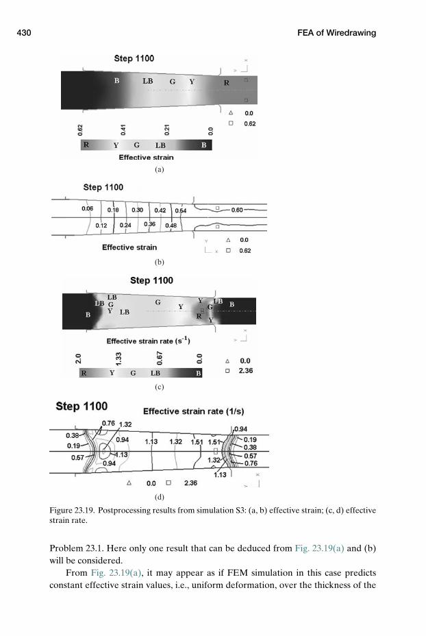
430 FEA of Wiredrawing
(a)
(b)
(c)
(d)
Figure 23.19. Postprocessing results from simulation S3: (a, b) effective strain; (c, d) effectivestrain rate.
Problem 23.1. Here only one result that can be deduced from Fig. 23.19(a) and (b)will be considered.
From Fig. 23.19(a), it may appear as if FEM simulation in this case predictsconstant effective strain values, i.e., uniform deformation, over the thickness of the
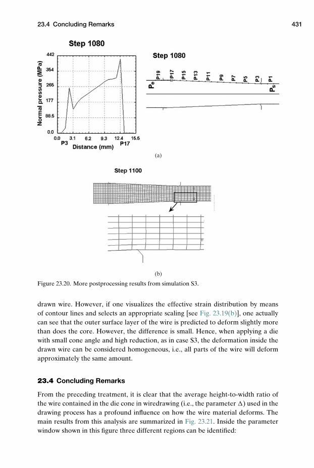
23.4 Concluding Remarks 431
(a)
(b)
Figure 23.20. More postprocessing results from simulation S3.
drawn wire. However, if one visualizes the effective strain distribution by meansof contour lines and selects an appropriate scaling [see Fig. 23.19(b)], one actuallycan see that the outer surface layer of the wire is predicted to deform slightly morethan does the core. However, the difference is small. Hence, when applying a diewith small cone angle and high reduction, as in case S3, the deformation inside thedrawn wire can be considered homogeneous, i.e., all parts of the wire will deformapproximately the same amount.
23.4 Concluding Remarks
From the preceding treatment, it is clear that the average height-to-width ratio ofthe wire contained in the die cone in wiredrawing (i.e., the parameter �) used in thedrawing process has a profound influence on how the wire material deforms. Themain results from this analysis are summarized in Fig. 23.21. Inside the parameterwindow shown in this figure three different regions can be identified:
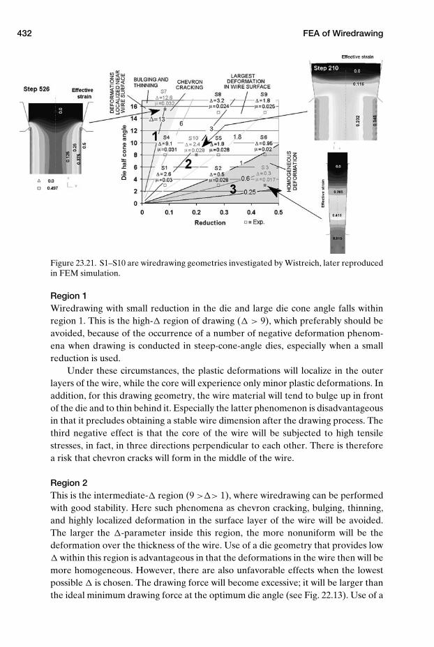
432 FEA of Wiredrawing
Figure 23.21. S1–S10 are wiredrawing geometries investigated by Wistreich, later reproducedin FEM simulation.
Region 1Wiredrawing with small reduction in the die and large die cone angle falls withinregion 1. This is the high-� region of drawing (� > 9), which preferably should beavoided, because of the occurrence of a number of negative deformation phenom-ena when drawing is conducted in steep-cone-angle dies, especially when a smallreduction is used.
Under these circumstances, the plastic deformations will localize in the outerlayers of the wire, while the core will experience only minor plastic deformations. Inaddition, for this drawing geometry, the wire material will tend to bulge up in frontof the die and to thin behind it. Especially the latter phenomenon is disadvantageousin that it precludes obtaining a stable wire dimension after the drawing process. Thethird negative effect is that the core of the wire will be subjected to high tensilestresses, in fact, in three directions perpendicular to each other. There is thereforea risk that chevron cracks will form in the middle of the wire.
Region 2This is the intermediate-� region (9 >�> 1), where wiredrawing can be performedwith good stability. Here such phenomena as chevron cracking, bulging, thinning,and highly localized deformation in the surface layer of the wire will be avoided.The larger the �-parameter inside this region, the more nonuniform will be thedeformation over the thickness of the wire. Use of a die geometry that provides low� within this region is advantageous in that the deformations in the wire then will bemore homogeneous. However, there are also unfavorable effects when the lowestpossible � is chosen. The drawing force will become excessive; it will be larger thanthe ideal minimum drawing force at the optimum die angle (see Fig. 22.13). Use of a
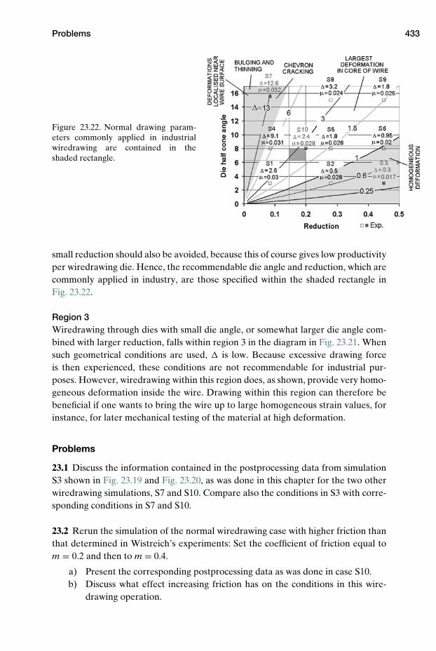
Problems 433
Figure 23.22. Normal drawing param-eters commonly applied in industrialwiredrawing are contained in theshaded rectangle.
small reduction should also be avoided, because this of course gives low productivityper wiredrawing die. Hence, the recommendable die angle and reduction, which arecommonly applied in industry, are those specified within the shaded rectangle inFig. 23.22.
Region 3Wiredrawing through dies with small die angle, or somewhat larger die angle com-bined with larger reduction, falls within region 3 in the diagram in Fig. 23.21. Whensuch geometrical conditions are used, � is low. Because excessive drawing forceis then experienced, these conditions are not recommendable for industrial pur-poses. However, wiredrawing within this region does, as shown, provide very homo-geneous deformation inside the wire. Drawing within this region can therefore bebeneficial if one wants to bring the wire up to large homogeneous strain values, forinstance, for later mechanical testing of the material at high deformation.
Problems
23.1 Discuss the information contained in the postprocessing data from simulationS3 shown in Fig. 23.19 and Fig. 23.20, as was done in this chapter for the two otherwiredrawing simulations, S7 and S10. Compare also the conditions in S3 with corre-sponding conditions in S7 and S10.
23.2 Rerun the simulation of the normal wiredrawing case with higher friction thanthat determined in Wistreich’s experiments: Set the coefficient of friction equal tom = 0.2 and then to m = 0.4.
a) Present the corresponding postprocessing data as was done in case S10.b) Discuss what effect increasing friction has on the conditions in this wire-
drawing operation.

434 FEA of Wiredrawing
23.3 Use simulation models S7 and S10 to compute the smallest principal stress inthe wire. Show the data as stress distributions inside the longitudinal section of thewire. Consider also the maximum principal stress distribution for the two cases pre-sented in Fig. 23.11 and Fig. 23.16.
a) Discuss the stress conditions in the center of the wire in these two cases.b) Try to find a good explanation why chevron cracks are likely to form in case
S7, while they are not in case S10.
NOTES
1. Wistreich, J. G.: “Investigation of the mechanics of wire drawing,” Proc. Inst. MechanicalEngineers, Vol. 169, 1955, pp. 654–665.
2. Valberg, H., and Wanheim, T.: “FE-analysis as a tool for the investigation of the mechan-ics of wire-drawing,” Int. J. Materials and Product Technology, Vol. 13, 1998, No. 3–6,pp. 234–265.
3. Avitzur, B.: “Study of flow through conical converging dies,” in “Metal Forming,” A. L.Hoffmanner (Ed.), Plenum Press, New York, 1971, pp. 1–46.

24 Sheet-Metal Forming
As pointed out previously in Ch. 2, sheet-metal forming differs a lot from bulk-metalforming in that the stress condition in a sheet-metal forming operation usually ischaracterized by tensile stress, whereas most commonly in bulk-metal forming thereis compressive stress. Because of this, necking and fracturing of the workpiece mate-rial is a much larger problem in sheet-metal forming than in bulk-metal forming. Auseful tool for optimization of sheet-metal forming processes, so that they can beconducted without problems due to necking or fracture, is circle grid analysis. Theprinciples applied in circle grid analysis will therefore be described in this chapter.After this, some technological test methods applied in order to test the formabilityof sheet metals will be described: plane strain stretching, biaxial stretching, and theErichsen test.
The principles used when forming-limit diagrams (FLDs) are made will beexplained. It will also be shown how such diagrams and circle grid analysis can beused in order to optimize the deformation conditions in a typical industrial sheet-metal forming operation.
Elastic springback is a phenomenon of great importance in sheet-metal forming.Commonly the cross section of the sheet does not become fully plasticized in suchprocesses. In bending, the midlayer of the sheet will deform elastically only, and willtherefore cause elastic springback in the material when the forming load is removed.
Sheet metals used for forming are commonly anisotropic, i.e., they have differ-ent properties in different directions. In the forthcoming sections, it will be shownhow such anisotropy can be described and quantified by measurements performedon sheet-metal specimens deformed in technological tests. Finally, the phenomenonof springback in sheet metals will be discussed in more depth. It will be shown howdifferent material and process parameters affect the amount of springback occurringin bending operations.
24.1 Circle Grid Analysis
The deformations that the workpiece is subjected to in sheet-metal forming can bequantified by means of circles on the surface of a sheet-metal specimen. Such circles
435
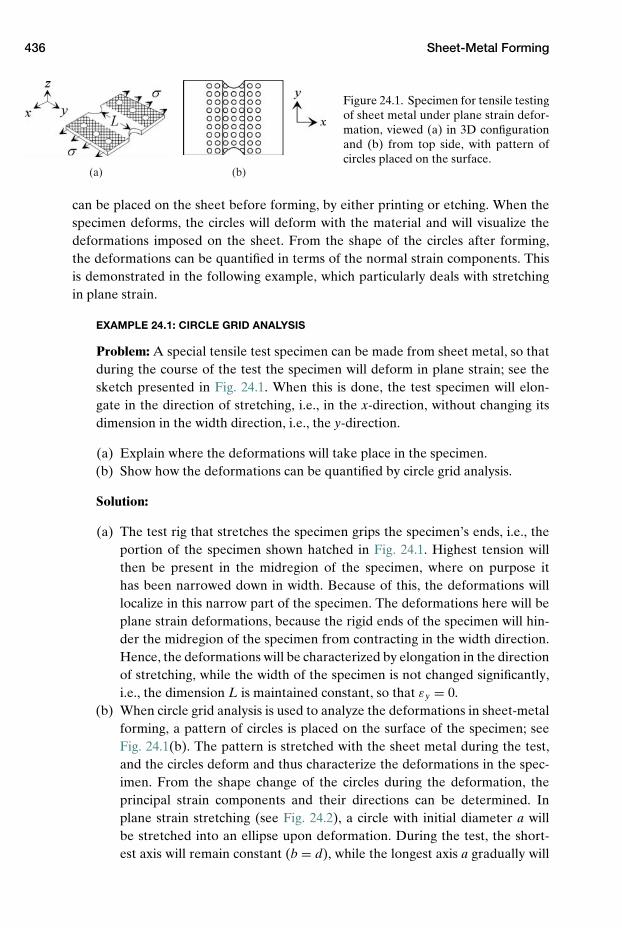
436 Sheet-Metal Forming
(a) (b)
Figure 24.1. Specimen for tensile testingof sheet metal under plane strain defor-mation, viewed (a) in 3D configurationand (b) from top side, with pattern ofcircles placed on the surface.
can be placed on the sheet before forming, by either printing or etching. When thespecimen deforms, the circles will deform with the material and will visualize thedeformations imposed on the sheet. From the shape of the circles after forming,the deformations can be quantified in terms of the normal strain components. Thisis demonstrated in the following example, which particularly deals with stretchingin plane strain.
EXAMPLE 24.1: CIRCLE GRID ANALYSIS
Problem: A special tensile test specimen can be made from sheet metal, so thatduring the course of the test the specimen will deform in plane strain; see thesketch presented in Fig. 24.1. When this is done, the test specimen will elon-gate in the direction of stretching, i.e., in the x-direction, without changing itsdimension in the width direction, i.e., the y-direction.
(a) Explain where the deformations will take place in the specimen.(b) Show how the deformations can be quantified by circle grid analysis.
Solution:
(a) The test rig that stretches the specimen grips the specimen’s ends, i.e., theportion of the specimen shown hatched in Fig. 24.1. Highest tension willthen be present in the midregion of the specimen, where on purpose ithas been narrowed down in width. Because of this, the deformations willlocalize in this narrow part of the specimen. The deformations here will beplane strain deformations, because the rigid ends of the specimen will hin-der the midregion of the specimen from contracting in the width direction.Hence, the deformations will be characterized by elongation in the directionof stretching, while the width of the specimen is not changed significantly,i.e., the dimension L is maintained constant, so that εy = 0.
(b) When circle grid analysis is used to analyze the deformations in sheet-metalforming, a pattern of circles is placed on the surface of the specimen; seeFig. 24.1(b). The pattern is stretched with the sheet metal during the test,and the circles deform and thus characterize the deformations in the spec-imen. From the shape change of the circles during the deformation, theprincipal strain components and their directions can be determined. Inplane strain stretching (see Fig. 24.2), a circle with initial diameter a willbe stretched into an ellipse upon deformation. During the test, the short-est axis will remain constant (b = d), while the longest axis a gradually will
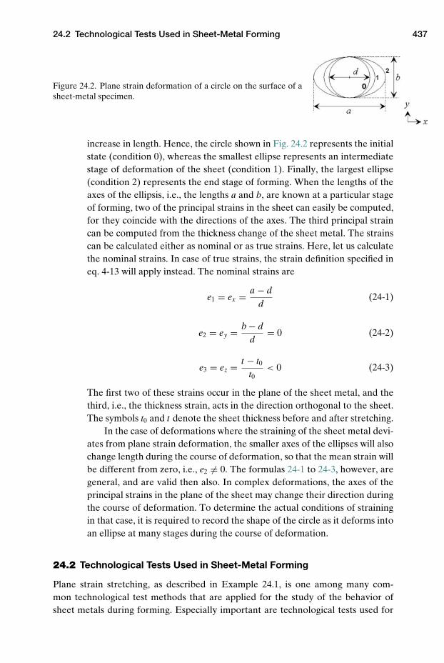
24.2 Technological Tests Used in Sheet-Metal Forming 437
Figure 24.2. Plane strain deformation of a circle on the surface of asheet-metal specimen.
increase in length. Hence, the circle shown in Fig. 24.2 represents the initialstate (condition 0), whereas the smallest ellipse represents an intermediatestage of deformation of the sheet (condition 1). Finally, the largest ellipse(condition 2) represents the end stage of forming. When the lengths of theaxes of the ellipsis, i.e., the lengths a and b, are known at a particular stageof forming, two of the principal strains in the sheet can easily be computed,for they coincide with the directions of the axes. The third principal straincan be computed from the thickness change of the sheet metal. The strainscan be calculated either as nominal or as true strains. Here, let us calculatethe nominal strains. In case of true strains, the strain definition specified ineq. 4-13 will apply instead. The nominal strains are
e1 = ex = a − dd
(24-1)
e2 = ey = b − dd
= 0 (24-2)
e3 = ez = t − t0t0
< 0 (24-3)
The first two of these strains occur in the plane of the sheet metal, and thethird, i.e., the thickness strain, acts in the direction orthogonal to the sheet.The symbols t0 and t denote the sheet thickness before and after stretching.
In the case of deformations where the straining of the sheet metal devi-ates from plane strain deformation, the smaller axes of the ellipses will alsochange length during the course of deformation, so that the mean strain willbe different from zero, i.e., e2 �= 0. The formulas 24-1 to 24-3, however, aregeneral, and are valid then also. In complex deformations, the axes of theprincipal strains in the plane of the sheet may change their direction duringthe course of deformation. To determine the actual conditions of strainingin that case, it is required to record the shape of the circle as it deforms intoan ellipse at many stages during the course of deformation.
24.2 Technological Tests Used in Sheet-Metal Forming
Plane strain stretching, as described in Example 24.1, is one among many com-mon technological test methods that are applied for the study of the behavior ofsheet metals during forming. Especially important are technological tests used for
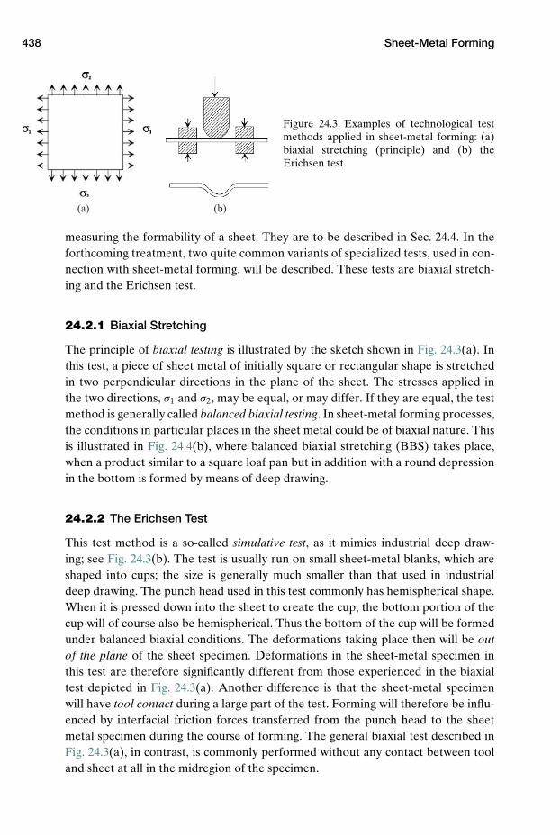
438 Sheet-Metal Forming
(a) (b)
Figure 24.3. Examples of technological testmethods applied in sheet-metal forming: (a)biaxial stretching (principle) and (b) theErichsen test.
measuring the formability of a sheet. They are to be described in Sec. 24.4. In theforthcoming treatment, two quite common variants of specialized tests, used in con-nection with sheet-metal forming, will be described. These tests are biaxial stretch-ing and the Erichsen test.
24.2.1 Biaxial Stretching
The principle of biaxial testing is illustrated by the sketch shown in Fig. 24.3(a). Inthis test, a piece of sheet metal of initially square or rectangular shape is stretchedin two perpendicular directions in the plane of the sheet. The stresses applied inthe two directions, σ1 and σ2, may be equal, or may differ. If they are equal, the testmethod is generally called balanced biaxial testing. In sheet-metal forming processes,the conditions in particular places in the sheet metal could be of biaxial nature. Thisis illustrated in Fig. 24.4(b), where balanced biaxial stretching (BBS) takes place,when a product similar to a square loaf pan but in addition with a round depressionin the bottom is formed by means of deep drawing.
24.2.2 The Erichsen Test
This test method is a so-called simulative test, as it mimics industrial deep draw-ing; see Fig. 24.3(b). The test is usually run on small sheet-metal blanks, which areshaped into cups; the size is generally much smaller than that used in industrialdeep drawing. The punch head used in this test commonly has hemispherical shape.When it is pressed down into the sheet to create the cup, the bottom portion of thecup will of course also be hemispherical. Thus the bottom of the cup will be formedunder balanced biaxial conditions. The deformations taking place then will be outof the plane of the sheet specimen. Deformations in the sheet-metal specimen inthis test are therefore significantly different from those experienced in the biaxialtest depicted in Fig. 24.3(a). Another difference is that the sheet-metal specimenwill have tool contact during a large part of the test. Forming will therefore be influ-enced by interfacial friction forces transferred from the punch head to the sheetmetal specimen during the course of forming. The general biaxial test described inFig. 24.3(a), in contrast, is commonly performed without any contact between tooland sheet at all in the midregion of the specimen.
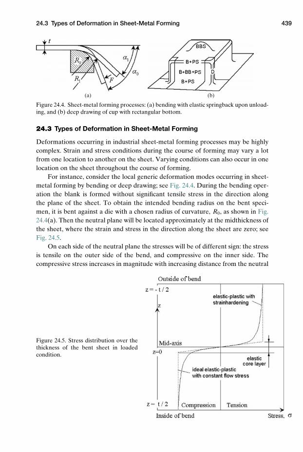
24.3 Types of Deformation in Sheet-Metal Forming 439
(a) (b)
Figure 24.4. Sheet-metal forming processes: (a) bending with elastic springback upon unload-ing, and (b) deep drawing of cup with rectangular bottom.
24.3 Types of Deformation in Sheet-Metal Forming
Deformations occurring in industrial sheet-metal forming processes may be highlycomplex. Strain and stress conditions during the course of forming may vary a lotfrom one location to another on the sheet. Varying conditions can also occur in onelocation on the sheet throughout the course of forming.
For instance, consider the local generic deformation modes occurring in sheet-metal forming by bending or deep drawing; see Fig. 24.4. During the bending oper-ation the blank is formed without significant tensile stress in the direction alongthe plane of the sheet. To obtain the intended bending radius on the bent speci-men, it is bent against a die with a chosen radius of curvature, R0, as shown in Fig.24.4(a). Then the neutral plane will be located approximately at the midthickness ofthe sheet, where the strain and stress in the direction along the sheet are zero; seeFig. 24.5.
On each side of the neutral plane the stresses will be of different sign: the stressis tensile on the outer side of the bend, and compressive on the inner side. Thecompressive stress increases in magnitude with increasing distance from the neutral
Figure 24.5. Stress distribution over thethickness of the bent sheet in loadedcondition.
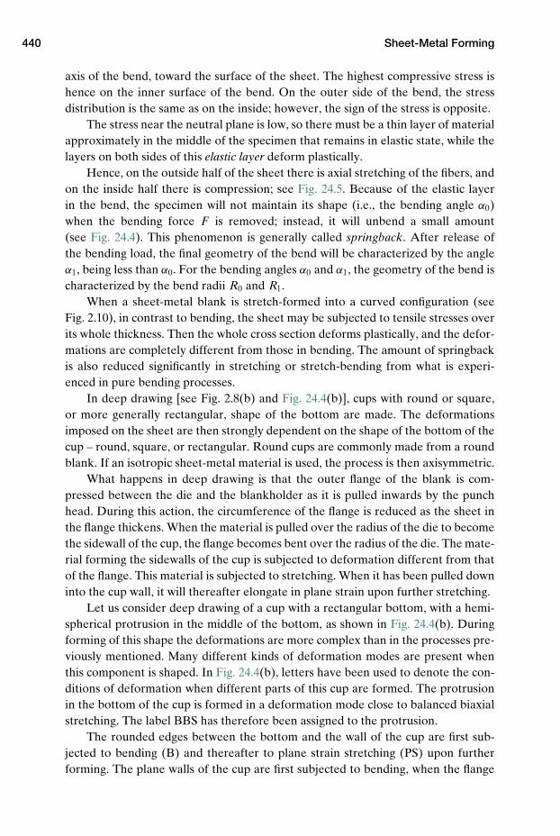
440 Sheet-Metal Forming
axis of the bend, toward the surface of the sheet. The highest compressive stress ishence on the inner surface of the bend. On the outer side of the bend, the stressdistribution is the same as on the inside; however, the sign of the stress is opposite.
The stress near the neutral plane is low, so there must be a thin layer of materialapproximately in the middle of the specimen that remains in elastic state, while thelayers on both sides of this elastic layer deform plastically.
Hence, on the outside half of the sheet there is axial stretching of the fibers, andon the inside half there is compression; see Fig. 24.5. Because of the elastic layerin the bend, the specimen will not maintain its shape (i.e., the bending angle α0)when the bending force F is removed; instead, it will unbend a small amount(see Fig. 24.4). This phenomenon is generally called springback. After release ofthe bending load, the final geometry of the bend will be characterized by the angleα1, being less than α0. For the bending angles α0 and α1, the geometry of the bend ischaracterized by the bend radii R0 and R1.
When a sheet-metal blank is stretch-formed into a curved configuration (seeFig. 2.10), in contrast to bending, the sheet may be subjected to tensile stresses overits whole thickness. Then the whole cross section deforms plastically, and the defor-mations are completely different from those in bending. The amount of springbackis also reduced significantly in stretching or stretch-bending from what is experi-enced in pure bending processes.
In deep drawing [see Fig. 2.8(b) and Fig. 24.4(b)], cups with round or square,or more generally rectangular, shape of the bottom are made. The deformationsimposed on the sheet are then strongly dependent on the shape of the bottom of thecup – round, square, or rectangular. Round cups are commonly made from a roundblank. If an isotropic sheet-metal material is used, the process is then axisymmetric.
What happens in deep drawing is that the outer flange of the blank is com-pressed between the die and the blankholder as it is pulled inwards by the punchhead. During this action, the circumference of the flange is reduced as the sheet inthe flange thickens. When the material is pulled over the radius of the die to becomethe sidewall of the cup, the flange becomes bent over the radius of the die. The mate-rial forming the sidewalls of the cup is subjected to deformation different from thatof the flange. This material is subjected to stretching. When it has been pulled downinto the cup wall, it will thereafter elongate in plane strain upon further stretching.
Let us consider deep drawing of a cup with a rectangular bottom, with a hemi-spherical protrusion in the middle of the bottom, as shown in Fig. 24.4(b). Duringforming of this shape the deformations are more complex than in the processes pre-viously mentioned. Many different kinds of deformation modes are present whenthis component is shaped. In Fig. 24.4(b), letters have been used to denote the con-ditions of deformation when different parts of this cup are formed. The protrusionin the bottom of the cup is formed in a deformation mode close to balanced biaxialstretching. The label BBS has therefore been assigned to the protrusion.
The rounded edges between the bottom and the wall of the cup are first sub-jected to bending (B) and thereafter to plane strain stretching (PS) upon furtherforming. The plane walls of the cup are first subjected to bending, when the flange
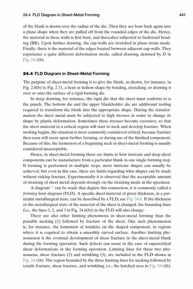
24.4 FLD Diagram in Sheet-Metal Forming 441
of the blank is drawn over the radius of the die. Then they are bent back again intoa plane shape when they are pulled off from the rounded edges of the die. Hence,the material in these walls is first bent, and thereafter subjected to backward bend-ing (BB). Upon further drawing, the cup walls are stretched in plane strain mode.Finally, there is the material of the edges located between adjacent cup walls. Theyexperience a quite different deformation mode, called drawing, denoted by D inFig. 24.4(b).
24.4 FLD Diagram in Sheet-Metal Forming
The purpose of sheet-metal forming is to give the blank, as shown, for instance, inFig. 2.8(b) to Fig. 2.11, a bent or hollow shape by bending, stretching, or drawing itover or onto the surface of a rigid forming die.
In deep drawing, for instance, the rigid die that the sheet must conform to isthe punch. The bottom die and the upper blankholder die are additional toolingrequired to transform the blank into the appropriate shape. During the transfor-mation the sheet metal must be subjected to high stresses in order to change itsshape by plastic deformation. Sometimes these stresses become excessive, so thatthe sheet material in a critical region will start to neck and develop fracture. Whennecking begins, the situation is most commonly considered critical, because fracturethen soon will occur upon further forming, or during use of the finished component.Because of this, the formation of a beginning neck in sheet-metal forming is usuallyconsidered unacceptable.
Hence, in sheet-metal forming there are limits to how intricate and deep sheetcomponents can be manufacture from a particular blank in one single forming step.If forming is performed in multiple steps, more intricate shapes can usually beachieved, but even in this case, there are limits regarding what shapes can be madewithout risking fracture. Experimentally it is observed that the acceptable amountof straining of sheet metal depends strongly on the straining mode in the specimen.
A diagram1,2 can be made that depicts this connection; it is commonly called aforming limit diagram (FLD). A specific sheet material of given thickness, in a par-ticular metallurgical state, can be described by a FLD; see Fig. 24.6. If the thicknessor the metallurgical state of the material of the sheet is changed, the bounding lines(i.e., the lines 1, 2, and 3 in Fig. 24.6(b)) in the FLD will also change.
There are also other limiting phenomena in sheet-metal forming than thepossible necking (1) followed by fracture of the sheet. One such phenomenonis, for instance, the formation of wrinkles on the shaped component, in regionswhere it is required to obtain a smoothly curved surface. Another limiting phe-nomenon is the eventual development of shear fracture in the sheet-metal blankduring the forming operation. Such defects can occur in the case of supercriticalshear deformations in the forming operation. Limiting lines for these two phe-nomena, shear fracture (2) and wrinkling (3), are included in the FLD shown inFig. 24.6(b). The region bounded by the three limiting lines for necking followed bytensile fracture, shear fracture, and wrinkling, i.e., the hatched area in Fig. 24.6(b),
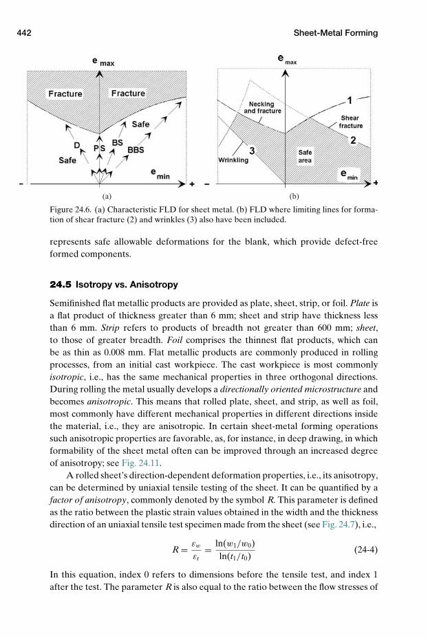
442 Sheet-Metal Forming
(a) (b)
Figure 24.6. (a) Characteristic FLD for sheet metal. (b) FLD where limiting lines for forma-tion of shear fracture (2) and wrinkles (3) also have been included.
represents safe allowable deformations for the blank, which provide defect-freeformed components.
24.5 Isotropy vs. Anisotropy
Semifinished flat metallic products are provided as plate, sheet, strip, or foil. Plate isa flat product of thickness greater than 6 mm; sheet and strip have thickness lessthan 6 mm. Strip refers to products of breadth not greater than 600 mm; sheet,to those of greater breadth. Foil comprises the thinnest flat products, which canbe as thin as 0.008 mm. Flat metallic products are commonly produced in rollingprocesses, from an initial cast workpiece. The cast workpiece is most commonlyisotropic, i.e., has the same mechanical properties in three orthogonal directions.During rolling the metal usually develops a directionally oriented microstructure andbecomes anisotropic. This means that rolled plate, sheet, and strip, as well as foil,most commonly have different mechanical properties in different directions insidethe material, i.e., they are anisotropic. In certain sheet-metal forming operationssuch anisotropic properties are favorable, as, for instance, in deep drawing, in whichformability of the sheet metal often can be improved through an increased degreeof anisotropy; see Fig. 24.11.
A rolled sheet’s direction-dependent deformation properties, i.e., its anisotropy,can be determined by uniaxial tensile testing of the sheet. It can be quantified by afactor of anisotropy, commonly denoted by the symbol R. This parameter is definedas the ratio between the plastic strain values obtained in the width and the thicknessdirection of an uniaxial tensile test specimen made from the sheet (see Fig. 24.7), i.e.,
R = εw
εt= ln(w1/w0)
ln(t1/t0)(24-4)
In this equation, index 0 refers to dimensions before the tensile test, and index 1after the test. The parameter R is also equal to the ratio between the flow stresses of
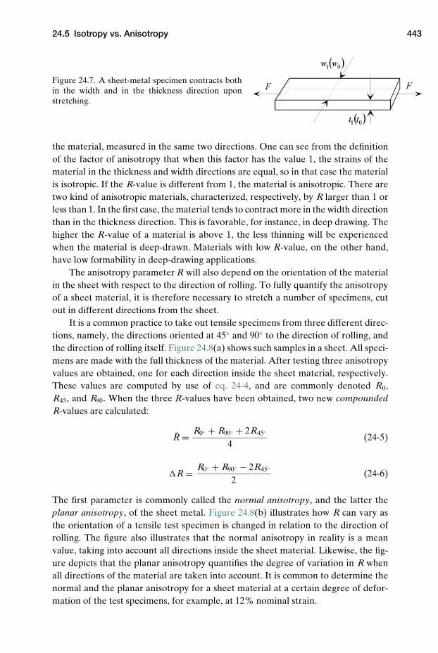
24.5 Isotropy vs. Anisotropy 443
Figure 24.7. A sheet-metal specimen contracts bothin the width and in the thickness direction uponstretching.
the material, measured in the same two directions. One can see from the definitionof the factor of anisotropy that when this factor has the value 1, the strains of thematerial in the thickness and width directions are equal, so in that case the materialis isotropic. If the R-value is different from 1, the material is anisotropic. There aretwo kind of anisotropic materials, characterized, respectively, by R larger than 1 orless than 1. In the first case, the material tends to contract more in the width directionthan in the thickness direction. This is favorable, for instance, in deep drawing. Thehigher the R-value of a material is above 1, the less thinning will be experiencedwhen the material is deep-drawn. Materials with low R-value, on the other hand,have low formability in deep-drawing applications.
The anisotropy parameter R will also depend on the orientation of the materialin the sheet with respect to the direction of rolling. To fully quantify the anisotropyof a sheet material, it is therefore necessary to stretch a number of specimens, cutout in different directions from the sheet.
It is a common practice to take out tensile specimens from three different direc-tions, namely, the directions oriented at 45◦ and 90◦ to the direction of rolling, andthe direction of rolling itself. Figure 24.8(a) shows such samples in a sheet. All speci-mens are made with the full thickness of the material. After testing three anisotropyvalues are obtained, one for each direction inside the sheet material, respectively.These values are computed by use of eq. 24-4, and are commonly denoted R0,R45, and R90. When the three R-values have been obtained, two new compoundedR-values are calculated:
R = R0◦ + R90◦ + 2R45◦
4(24-5)
�R = R0◦ + R90◦ − 2R45◦
2(24-6)
The first parameter is commonly called the normal anisotropy, and the latter theplanar anisotropy, of the sheet metal. Figure 24.8(b) illustrates how R can vary asthe orientation of a tensile test specimen is changed in relation to the direction ofrolling. The figure also illustrates that the normal anisotropy in reality is a meanvalue, taking into account all directions inside the sheet material. Likewise, the fig-ure depicts that the planar anisotropy quantifies the degree of variation in R whenall directions of the material are taken into account. It is common to determine thenormal and the planar anisotropy for a sheet material at a certain degree of defor-mation of the test specimens, for example, at 12% nominal strain.
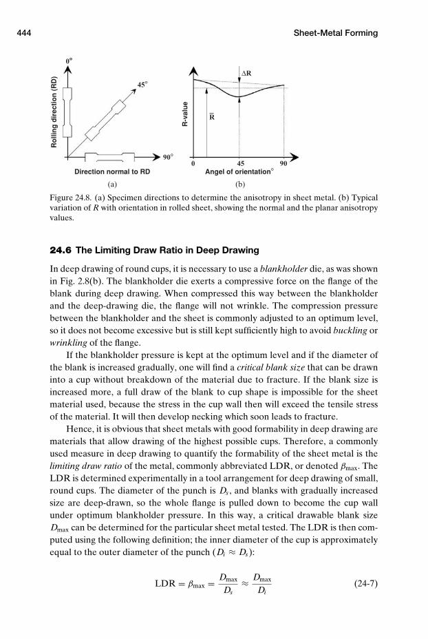
444 Sheet-Metal Forming
0°°
45°
90°0 45 90
∆R
R
Direction normal to RD Angel of orientation°
Ro
llin
g d
irec
tio
n (
RD
)
R-v
alu
e(a) (b)
Figure 24.8. (a) Specimen directions to determine the anisotropy in sheet metal. (b) Typicalvariation of R with orientation in rolled sheet, showing the normal and the planar anisotropyvalues.
24.6 The Limiting Draw Ratio in Deep Drawing
In deep drawing of round cups, it is necessary to use a blankholder die, as was shownin Fig. 2.8(b). The blankholder die exerts a compressive force on the flange of theblank during deep drawing. When compressed this way between the blankholderand the deep-drawing die, the flange will not wrinkle. The compression pressurebetween the blankholder and the sheet is commonly adjusted to an optimum level,so it does not become excessive but is still kept sufficiently high to avoid buckling orwrinkling of the flange.
If the blankholder pressure is kept at the optimum level and if the diameter ofthe blank is increased gradually, one will find a critical blank size that can be drawninto a cup without breakdown of the material due to fracture. If the blank size isincreased more, a full draw of the blank to cup shape is impossible for the sheetmaterial used, because the stress in the cup wall then will exceed the tensile stressof the material. It will then develop necking which soon leads to fracture.
Hence, it is obvious that sheet metals with good formability in deep drawing arematerials that allow drawing of the highest possible cups. Therefore, a commonlyused measure in deep drawing to quantify the formability of the sheet metal is thelimiting draw ratio of the metal, commonly abbreviated LDR, or denoted βmax. TheLDR is determined experimentally in a tool arrangement for deep drawing of small,round cups. The diameter of the punch is Ds , and blanks with gradually increasedsize are deep-drawn, so the whole flange is pulled down to become the cup wallunder optimum blankholder pressure. In this way, a critical drawable blank sizeDmax can be determined for the particular sheet metal tested. The LDR is then com-puted using the following definition; the inner diameter of the cup is approximatelyequal to the outer diameter of the punch (Di ≈ Ds):
LDR = βmax = Dmax
Ds≈ Dmax
Di(24-7)
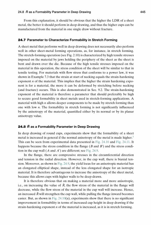
24.8 R as a Formability Parameter in Deep Drawing 445
From this explanation, it should be obvious that the higher the LDR of a sheetmetal, the better it should perform in deep drawing, and thus the higher cups can bemanufactured from the material in one single draw without fracture.
24.7 Parameter to Characterize Formability in Stretch Forming
A sheet metal that performs well in deep drawing does not necessarily also performwell in other sheet-metal forming operations, as, for instance, in stretch forming.The stretch-forming operation (see Fig. 2.10) is characterized by high tensile stressesimposed on the material by jaws holding the periphery of the sheet as the sheet isbent and drawn over the die. Because of the high tensile stresses imposed on thematerial in this operation, the stress condition of the sheet will be similar to that intensile testing. For materials with flow stress that conforms to a power law, it wasshown in Example 7.3 that the strain at start of necking equals the strain-hardeningexponent n of the material. This implies that the higher the strain hardening expo-nent is for a material, the more it can be deformed by stretching before necking(and fracture) occurs. This is also demonstrated in Sec. 9.2. The strain-hardeningexponent of the material is therefore a parameter that should preferably be highto secure good formability in sheet metals used in stretch-forming applications. Amaterial with high n allows deeper components to be made by stretch forming thanone with low n. The formability in stretch forming is not significantly influencedby the anisotropy of the material, quantified either by its normal or by its planaranisotropy value.
24.8 R as a Formability Parameter in Deep Drawing
In deep drawing of round cups, experiments show that the formability of a sheetmetal is increased in general if the normal anisotropy of the metal is made higher.3
This can be seen from experimental data presented in Fig. 24.10 and Fig. 24.11. Ithappens because the stress condition in the flange (B and B′) and the stress condi-tion in the cup wall (A and A′) are different; see Fig. 24.9.
In the flange, there are compressive stresses in the circumferential directionand tension in the radial direction. However, in the cup wall, there is biaxial ten-sion. Moreover, as shown in Fig. 24.9, the yield locus for an anisotropic material hasan elongated elliptical shape, instead of the less elongated shape for an isotropicmaterial. It is therefore advantageous to increase the anisotropy of the sheet metal,because this allows cups with higher walls to be deep-drawn.
It is therefore obvious that on making a material more and more anisotropic,i.e., on increasing the value of R, the flow stress of the material in the flange willdecrease, while the flow stress of the material in the cup wall will increase. Hence,an increased R will strengthen the cup wall, while pulling the flange inward becomeseasier. But, as shown in Fig. 24.10(a), experiments show that there is no significantimprovement in formability in terms of increased cup height in deep drawing if thestrain-hardening exponent n of the material is increased, as it is in stretch forming.
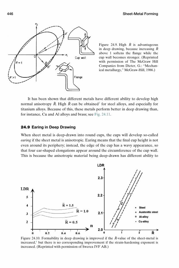
446 Sheet-Metal Forming
Figure 24.9. High R is advantageousin deep drawing, because increasing Rabove 1 softens the flange while thecup wall becomes stronger. (Reprintedwith permission of The McGraw HillCompanies from Dieter, G.: “Mechan-ical metallurgy,” McGraw-Hill, 1986.)
It has been shown that different metals have different ability to develop highnormal anisotropy R. High R can be obtained3 for steel alloys, and especially fortitanium alloys. Because of this, these metals perform better in deep drawing than,for instance, Cu and Al alloys and brass; see Fig. 24.11.
24.9 Earing in Deep Drawing
When sheet metal is deep-drawn into round cups, the cups will develop so-calledearing if the sheet metal is anisotropic. Earing means that the final cup height is noteven around its periphery; instead, the edge of the cup has a wavy appearance, sothat four ear-shaped elongations appear around the circumference of the cup wall.This is because the anisotropic material being deep-drawn has different ability to
Figure 24.10. Formability in deep drawing is improved if the R-value of the sheet-metal isincreased,4 but there is no corresponding improvement if the strain-hardening exponent isincreased. (Reprinted with permission of Swerea IVF AB.)
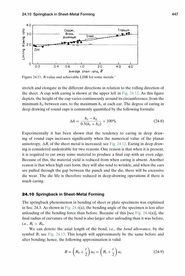
24.10 Springback in Sheet-Metal Forming 447
Figure 24.11. R-value and achievable LDR for some metals.5
stretch and elongate in the different directions in relation to the rolling direction ofthe sheet. A cup with earing is shown at the upper left in Fig. 24.12. As this figuredepicts, the height of the cup varies continuously around its circumference, from theminimum hd between ears, to the maximum he at each ear. The degree of earing indeep drawing of round cups is commonly quantified by the following formula:
�h = he − hd
0.5(he + hd)× 100% (24-8)
Experimentally it has been shown that the tendency to earing in deep draw-ing of round cups increases significantly when the numerical value of the planaranisotropy, �R, of the sheet metal is increased; see Fig. 24.12. Earing in deep draw-ing is considered undesirable for two reasons. One reason is that when it is present,it is required to cut away some material to produce a final cup with an even edge.Because of this, the material yield is reduced from when earing is absent. Anotherreason is that when high ears form, they will also tend to wrinkle, and when the earsare pulled through the gap between the punch and the die, there will be excessivedie wear. The die life is therefore reduced in deep-drawing operations if there ismuch earing.
24.10 Springback in Sheet-Metal Forming
The springback phenomenon in bending of sheet or plate specimens was explainedin Sec. 24.3. As shown in Fig. 24.4(a), the bending angle of the specimen is less afterunloading of the bending force than before. Because of this [see Fig. 24.4(a)], thefinal radius of curvature of the bend is also larger after unloading than it was before,i.e., R1 > R0.
We can denote the axial length of the bend, i.e., the bend allowance, by thesymbol B; see Fig. 24.13. This length will approximately be the same before andafter bending; hence, the following approximation is valid:
B =(
R0 + t2
)α0 =
(R1 + t
2
)α1 (24-9)
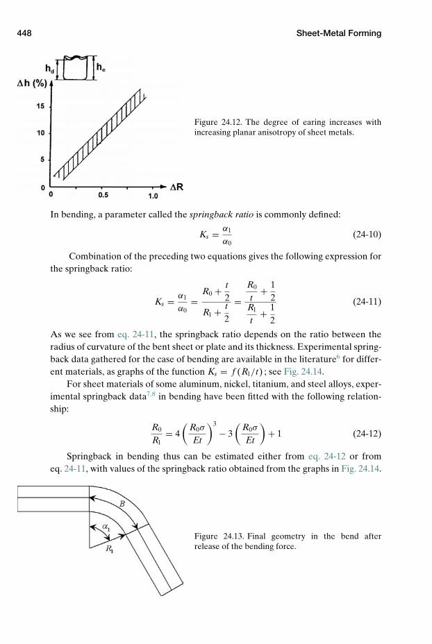
448 Sheet-Metal Forming
Figure 24.12. The degree of earing increases withincreasing planar anisotropy of sheet metals.
In bending, a parameter called the springback ratio is commonly defined:
Ks = α1
α0(24-10)
Combination of the preceding two equations gives the following expression forthe springback ratio:
Ks = α1
α0=
R0 + t2
R1 + t2
=R0
t+ 1
2R1
t+ 1
2
(24-11)
As we see from eq. 24-11, the springback ratio depends on the ratio between theradius of curvature of the bent sheet or plate and its thickness. Experimental spring-back data gathered for the case of bending are available in the literature6 for differ-ent materials, as graphs of the function Ks = f (R1/t) ; see Fig. 24.14.
For sheet materials of some aluminum, nickel, titanium, and steel alloys, exper-imental springback data7,8 in bending have been fitted with the following relation-ship:
R0
R1= 4
(R0σ
Et
)3
− 3(
R0σ
Et
)+ 1 (24-12)
Springback in bending thus can be estimated either from eq. 24-12 or fromeq. 24-11, with values of the springback ratio obtained from the graphs in Fig. 24.14.
Figure 24.13. Final geometry in the bend afterrelease of the bending force.
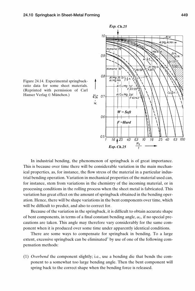
24.10 Springback in Sheet-Metal Forming 449
Figure 24.14. Experimental springback-ratio data for some sheet materials.(Reprinted with permission of CarlHanser Verlag c© Munchen.)
In industrial bending, the phenomenon of springback is of great importance.This is because over time there will be considerable variation in the main mechan-ical properties, as, for instance, the flow stress of the material in a particular indus-trial bending operation. Variation in mechanical properties of the material used can,for instance, stem from variations in the chemistry of the incoming material, or inprocessing conditions in the rolling process when the sheet metal is fabricated. Thisvariation has great effect on the amount of springback obtained in the bending oper-ation. Hence, there will be shape variations in the bent components over time, whichwill be difficult to predict, and also to correct for.
Because of the variation in the springback, it is difficult to obtain accurate shapeof bent components, in terms of a final constant bending angle, α1, if no special pre-cautions are taken. This angle may therefore vary considerably for the same com-ponent when it is produced over some time under apparently identical conditions.
There are some ways to compensate for springback in bending. To a largeextent, excessive springback can be eliminated9 by use of one of the following com-pensation methods:
(1) Overbend the component slightly; i.e., use a bending die that bends the com-ponent to a somewhat too large bending angle. Then the bent component willspring back to the correct shape when the bending force is released.
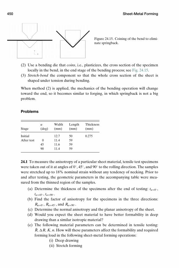
450 Sheet-Metal Forming
Figure 24.15. Coining of the bend to elimi-nate springback.
(2) Use a bending die that coins, i.e., plasticizes, the cross section of the specimenlocally in the bend, in the end stage of the bending process; see Fig. 24.15.
(3) Stretch-bend the component so that the whole cross section of the sheet isshaped under tension during bending.
When method (2) is applied, the mechanics of the bending operation will changetoward the end, so it becomes similar to forging, in which springback is not a bigproblem.
Problems
α Width Length ThicknessStage (deg) (mm) (mm) (mm)
Initial 12.7 50 0.275After test 0 11.4 59
45 11.6 5990 11.4 59
24.1 To measure the anisotropy of a particular sheet material, tensile test specimenswere taken out of it at angles of 0◦, 45◦, and 90◦ to the rolling direction. The sampleswere stretched up to 18% nominal strain without any tendency of necking. Prior toand after testing, the geometric parameters in the accompanying table were mea-sured from the thinned region of the samples.
(a) Determine the thickness of the specimens after the end of testing: tα=0◦ ,tα=45◦ , tα=90◦ .
(b) Find the factor of anisotropy for the specimens in the three directions:Rα=0◦ , Rα=45◦ , and Rα=90◦ .
(c) Determine the normal anisotropy and the planar anisotropy of the sheet.(d) Would you expect the sheet material to have better formability in deep
drawing than a similar isotropic material?(e) The following material parameters can be determined in tensile testing:
R,�R, K, n. How will these parameters affect the formability and requiredforming load in the following sheet-metal forming operations:
(i) Deep drawing(ii) Stretch forming
References 451
24.2 Describe as briefly as possible, but completely, how the normal anisotropy andthe planar anisotropy of a rolled plate are determined.
24.3 The anisotropic properties of a plate are determined to be �R = 0.2 and R =2.2. A round cup of 300 mm diameter is to be produced from this plate by means ofdeep drawing.
(a) Determine the height of the highest possible cup that can be made from thisplate in a single deep drawing operation. Assume that the wall-thickness ofthe cup remains constant and equal to the thickness of the plate over thewhole cup wall.
(b) Specify the maximum cup height that can be made, as a fraction of the innerdiameter of the cup. Discuss the validity of the assumption made.
(c) Determine the height of the ears obtained on the resulting cup.
NOTES
1. Keeler, S. P.: “Rating the formability of sheet metal,” Metals Progress, Oct. 1966,pp. 148–153.
2. Goodwin, G. M.: “Application of strain analysis to sheet metal problems in press shop,”Metallurgica Italiana, Vol. 60, 1968, pp. 767–774.
3. Dieter, G.: “Mechanical Metallurgy,” McGraw-Hill, 1986.4. Weidemann, C.: “Determination of the deep drawability of materials,” Expert Confer-
ence, Lerum, Sweden, 14–15 Sept., 1972, Jernkontoret, Stockholm.5. Atkinson, M.: “Assessing normal anisotropic plasticity of sheet metals,” Sheet Metal
Industries, Vol. 44, 1967, pp. 167–178.6. Oehler, G.: “Biegen,” Hanser, Munchen, 1963 (in German).7. Gardiner, F. J.: “The springback of metals,” Trans. ASME, Vol. 79, 1957, pp. 1–9.8. Queener, C. A., and De Angelis, R. J.: “Elastic springback and residual stresses in sheet
metal formed by bending,” ASM Trans. Quarterly, Vol. 61, 1968, pp. 757–768.9. Kalpakjian, S., and Schmid, S. R.: “Manufacturing Processes for Engineering Materials,”
5th ed., Prentice-Hall, 2008, p. 410.
REFERENCES
Boljanovic, V.: “Sheet Metal Forming Processes and Design,” Industrial Press, New York,2004.
Hu, J., Marciniak, Z., and Duncan, J.: “Mechanics of Sheet Metal Forming,” 2nd ed.,Butterworth-Heinemann, 2002.
Oehler, G.: “Bending,” Hanser Verlag, Munchen, 1963.Szumera, J.: “The Metal Stamping Process: Your Product from Concept to Customer,” Indus-
trial Press, New York, 2002.


Index
accumulation of outer layer of billet in discard,322
adaptive remeshing, 223adhesion of lubricant to workpiece, 146advantage and disadvantage of backward
extrusion, 24, 324allotropic behavior of steel, 118analogy, between stress and strain, 62,
66anisotropy
factor of, 442measurement, 443normal, 443planar, 443in sheet-metal, 442in worked metals, 7
area reduction, 77aspect ratio in
cylinder compression, 81plain strain compression, 35
asperity, 141plastification, 142
atoms, packing of, 3austenite, 118average
length strain, 78pressure in frictionless compression, 81
axi-symmetric FEM model, 225
back-pull in wiredrawing, 398backward cup extrusion
effective strain rate distribution, 286effective strain distribution, 288FEA of process, 285–301
balanced biaxial stretching, 438barreling of cylinder in compression, 108bearing in wiredrawing dies, 399bend allowance, 447bending, 28
of sheet-metal, 439biaxial stretching, 438
billet, 22removal without deformation, 350
blank holder, 27, 444blanking, 30
conventional, 30fine, 30
blister defect, 323, 331bloom, 22bottleneck in forming, 12boundary
film lubrication, 146, 147–149lubrication, 146
boundary conditions in FEA, 224breakdown of material, 127
due to cracking, 134breakdown of
cast microstructure, 4lubricant film, 13
Bridgman’sassumptions in necking analysis, 243correction factor in tensile testing, 105theoretical analysis of, 104
buckling, 19in deep-drawing, 444
bulging incylinder compression, 108wire drawing, 417, 418
bulk metal forming, 9, 18burp cycle, 332
calibration draw, 395capstan, 396casting
defect formation, 5material loss, 5
cast iron, 3cavity filling, 268cementite flakes 2, 3center bursts, 421center zone in plain strain compression, 41cermets, 398
453

454 Index
material model, 115chevron cracks, 421
growth in FEA, 423circle grid analysis, 435, 436
to determine strains, 68classification system
extrudability of Al-alloys, 335extrusion processes, 10metal forming, 9, 18shapes of Al-profiles, 334shapes of forgings, 271, 272subdivision metal forming processes, 10types of metal flow in extrusion, 326
clay, deformation of, 1deformation mechanism, 3
clean cut in shearing, 30cleaning, of surfaces, 144closed die forging, 20–21
die filling in, 302example of laboratory process, 302FEA of, 302–316optimized process, 279
Cockroft-Latham failure criterion, 134coefficient of friction, 142cogging, 20coiling of wire, 396cold drawing of wire, 27cold forming
cold working by wiredrawing, 27to gain high strength, 7temperature range of, 118vs. hot forming, 34
complex strain path in sheet-metal forming, 437compression
axial, 87homogeneous slab, 87retarded stroke for constant strain rate,
108compression testing, advantages over tensile
testing, 95compressive stress
on inside of bend, 439in wiredrawing die, 398
cone angle in wiredrawing, 400confinement of air in extrusion material, 332constancy of volume, 63
deviation from rule of, 64constitutive equation
definition, 115in cold forming, 118general expression, 117in hot forming, 122including microstructural mechanisms, 122metals in general, 115–118
contact angle in rolling, 370contact area
apparent area, 141in compression, 107real area, 141
contact conditions betweenbillet and container, in extrusion, 351roll and workpiece, in rolling, 365
contact mechanisms, workpiece-die, 143contact pressure against die as process parameter,
14contact pressure against die in
cylinder compression, 230–233deep drawing, 27from the slab method, 373light slab rolling, 380normal slab rolling, 387normal wiredrawing, 427strip rolling, 391wiredrawing, 400
contact zone againstdie in closed-die forging, 302–305
contaminationas subsurface defect in extrusion, 330of surfaces, 144
continuous casting, 22continuum
mechanics, 2medium, 2
converging channel of wiredrawing die, 399conversion coating, 300cooling
effects, 159, 162of plate against die, 163–164
copper wiredrawing, 414Coulomb friction
model, 140–142validity of model, 142
cracking, 127due to lamination, 8in cylinder bulge, 134, 136in shear, 136transverse cracking in extrusion, 134
critical blank size in deep-drawing, 444crystals, aggregate of, 3cup forming by deep drawing, 27curve fitting
applied for the flow stress, 118determination of constants, 119
cutting, 10cylinder compression
basic mechanics of test method, 106compression velocity, 106deformation in corner of bulge, 252deformations in compression test, 253–254dies applied in test, 106experimental set-up, 106FEA of test, 229flow curve in test, 107with friction, 108friction effects, 199friction measurement using pins, 153–154frictionless compression, 1homogeneous compression, 107, 251

Index 455
principal stress in frictionless case, 210reduced friction in test, 109strain rate field in frictionless case, 210as technological test, 93, 95velocity field in frictionless case, 209
damage parameter inlight slab rolling pass, 381normal slab rolling pass, 386normal wiredrawing from FEA, 427plain strain compression, 47small reduction, large cone angle wiredrawing,
421strip rolling pass, 392wiredrawing, 421
damage parameter, critical value, 134dead zone in
backward cup extrusion, 286cylinder compression, 109extrusion, 183, 322plain strain compression, 41strip rolling, 390
deep drawing, 27applied tooling, 27fracture in, 28of rectangular cup, 440of round cup, 440of sheet-metal, 439wrinkling, 28
defectsavoid defects because of economy, 14blisters in extrusion, 323of critical size, 130in forging, 279hot tearing in Al-extrusion, 159
DEFORM R©-code, 223FEM-approach used, 224
deformationcomparison of compression and tension, 59over edge of plain strain compression die, 44effect of varying clearance in shearing,
260–263elastic, 1energy, 160fluctuations in wiredrawing, 417homogeneity in cylinder compression, 108homogeneity in extrusion seam, 238of inhomogeneous nature, 2macroscopic, 2mapping of, 2mechanism of, 4microscopic, 3multiplication of deformation crosses, 46near punch in backward cup extrusion, 296patterns in wiredrawing, 431of permanent character, 116plastic, 1simple measure of total deformation, 77
deformation analysis, 40–46
deformation characteristics of extruded rod, 192deformation cross in
normal wiredrawing, 424plain strain compression, 44strip rolling, 390cylinder compression, 253
deformation fromdeformed grid pattern, 182effective strain distribution, 43effective strain rate distribution, 43grid pattern in backward extrusion, 290–292strain rate distribution in wiredrawing, 425velocity field, 85–87
deformation inbackward cup extrusion, 286deep-drawing, 440extruded rod from grid pattern, 192–195extruded rod, 361extrusion, 24extrusion billet from strain rate, 362front end of extruded rod, 322hot closed die forging, 310–314light pass slab rolling, 377, 379neck from circle pattern, 247necking section, 243neck in tensile test, 103normal pass slab rolling, 383plain strain compression test, 40–46shearing, 30, 259sheet-metal forming, 438strip rolling, 389wiredrawing, low reduction – large angle, 416wiredrawing, normal drawing geometry, 425
degree of reduction, 79deletion of FEM-mesh to model cracking, 422�-parameter, 81
in plain strain compression, 36in rolling, 376in strip rolling, 393in wiredrawing, 403, 414in Wistreich’s wiredrawing experiments,
414diamond in wiredrawing die, 398die bridge in extrusion, 333die cavity, 20die filling in closed-die forging, 277, 302die geometry, characteristic parameters, 400die-life, influenced by fatigue, 142die orifice, 23dies
in metal forming, 13wear of, 13
die splitting force instrip drawing, 149wiredrawing, 401, 414
diffuse necking, 131dimensional stability in drawing, 395direct contact between surfaces, 144directionally oriented microstructure, 442

456 Index
discardin extrusion, 321, 323removal of, 324
dislocation, 3density, 3movement, 3
dislocation networks in cold and hot forming,122
displacement components, 86division processes, shearing, 30draft in rolling, 383drawing
as continuous process, 396as discontinuous process, 396of strip, 64unit in wiredrawing machine, 397wheel, 396
drawing cell in drawing machine, 398drawing conditions in normal wiredrawing,
424ductility, 128
increase through metal working, 7
earingfactors influencing earing, 447phenomenon in deep-drawing, 446
ease of working, 128economy in metal forming, 14edges for cutting, 30effective strain distribution, plain strain
compression, 43effective strain rate distribution, plain strain
compression, 43elastic
layer in bend, 440zone, 191
elastic deformationof dies, 53in tensile test, 102
elasticity theory, 53elastic-plastic
materials, 116emissitivity, 164emptying diagram
in backward cup extrusion, 296concept, 195in extrusion made by FEA, 359
emptying linelongitudinal, 199transverse, 197
energy consumptiondefinition of, 69in extrusion, 325friction energy, 406for homogeneous deformation, 405for inhomogeneous deformation, 407–409total in wiredrawing, 405, 409
energy dissipation, 69entrance into roll gap, 376
equation to find friction in split die experiment,401
Erichsen-test, 438Eulerian description, 222eutectic phases, as contamination in extrusion, 324excessive stresses in sheet-metal forming, 441experiments to validate FEM analysis, 35explicit FEM-method, 222exponent of strain hardening, 118extrudability of
Al, 25Al-alloys, 335
extrudate, 320extruded profiles, 23extrusion, 23–26, 320
advantage of direct over indirect, 24backward process, 23billet, 23classification of processes, 10complex hollow profile extrusion, 25container, 23of copper and brass, 24defect, 331direct process, 23division into subprocesses, 326, 347flow of outer layer of billet, 24force, 337force against container wall, 338forward process, 23friction force, 341homogeneous deformation force, 341hot extrusion of Al, 322hot lubricated, 25indirect process, 23inhomogeneous deformation force, 342limitations in backward extrusion, 24of light metals, 24load in backward extrusion, 325metal flow in direct and indirect process, 24in multi-hole dies, 24peripheral billet layer, 24practice in forward extrusion, 323pressure, 337pressure welding, 25punch, 23ram, 23residue, 321, 323seam welds, 26shell extrusion, 24of steel, 25tooling in porthole die extrusion, 25total force, 337, 343welding, 26welding, FEM-model of, 233–238welding chamber, 25
failurecriteria, 134catastrophic, 130

Index 457
FEAcorrection of flow curve, 245–246to determine thermal effects, 168–173in general, 220general importance in metal forming, 221graphical presentation of results, 229results as parameter distribution, 229
FEM-codesdevelopment of, 221to model metal forming, 223
FEM model, 2Dbackward Al-extrusion, 358–362backward cup extrusion, 285–301cylinder compression, 136, 200–201, 229–233,
250–253extrusion welding, 237–238, 333forward Al-extrusion, 352–357forward extrusion, subprocesses,
347–349plain strain compression, 225, 226shearing, deformations in sheared layer,
257–263shearing, to find K and n, 264–265slab rolling pass, 376–393tensile test, formability consideration,
130–131tensile testing, risk of cracking, 135–136tensile testing, stress conditions in neck,
243–246wiredrawing, 415–431
FEM model, 3Dclosed-die forging, 302–316cylinder compression, 253extrusion welding, 233–237plain strain compression, 37–50tensile testing, necking, 247
FEM-modeling, in general, 220FEM-solver, 224ferrite, 2, 118finished product, 13finishing die, 274finite difference method, 204finite element analysis (FEA), 34
validation of, 35finite element method (FEM), 34finite elements, 221flash, 21
formation of, 4flash gap, 277
characteristic geometrical conditions, 281common designs, 281design rules in closed-die forging, 280
flash less forging, 20flat rolling, 22flat-faced die, in extrusion, 322FLD-diagram, 130, 441flow criteria, the von Mises and Tresca criterion,
111flow criterion, correctness of, 38
flow curve, 116determination in cold forming, 107determination curve in hot forming, 107from tensile test, 102true and nominal curve, 103
flow direction of outer layer of billet in extrusion,331
flow formulation, 222flow patterns in extrusion, 326–328flow rule of Levy-Mises, 73flow stress
of Al-alloys in bending experiments,in cold, warm, and hot forming, 115, 116from compression test, 107of copper wire, 117, 416general function, 118to get right metal flow in Al-extrusion,
353mean value of in wiredrawing, 405parameter influence, 116as process parameter, 14from shearing test, 263–265temperature dependence, 117variation due to microstructure, 118
flow types in extrusion, 190foil, 442folds, 279force
on the roll, 367total force in wiredrawing, 399
forgeability, 269of different metals, 270
forgingas a requirement, 7avoiding unsound grain flow, 8as nonstationary process, 85deformation in hot closed die forging,
310–314design of multistep series, 274–276design principles, 276design to avoid defects, 280to improve fatigue resistance, 8mass distribution principle in, 276optimum temperature, 269stock, 274typical multi-step forging sequence, 275
forgingscomplexity of, 271shapes difficulty to forge, 272
formability, 127to avoid defect formation, 14improvements in deep-drawing, 442limits, 441of metals in deep-drawing, 446parameter in deep-drawing, 445parameter in stretch forming, 445
forming undercompressive stress, 9, 18tensile stress, 9, 18

458 Index
fracture, 127elongation, 94, 103in forgings due to defects, 280in shear, 138strain, 94, 103
free forming, 19friction
in backward cup extrusion, 300Causing load increase in bending, 216determination in plain strain compression, 37dry friction, 144–145effects in metal forming, 139effects on flow curve from compression,
254energy dissipation, 162factor, 143force, 141force as process parameter, 14heating, 161hill, 208influence on forming load, 139measurement in forming, 149–155measurement in wiredrawing, 400measurement using pins, 152shear stress, 142shear stress in wiredrawing, 400from surface ring pattern, 199
friction coefficient, 142value, boundary film lubrication, 148value, hydrodynamic lubrication, 147
frictionless compression, average pressure vs. �,81
friction models, 140comparison of models, 143implementation of in FEM-codes, 229
full separation of contact surfaces, 144fusion welding, 26
general extrusion, part of extrusion process, 349generic deformation modes in sheet-metal
forming, 439Gleeble simulator, 96
testing, 35working principle of simulator, 96
grainboundaries, 2as crystals, 3flow in forgings, 8
graphical tools in FEM analysis, 224grid pattern analysis
in compression experiment, 249deformation of grid elements, 41in extrusion welding, 237in FEA of compression, 250in shearing experiment, 259
grid pattern distortions inbackward Al-extrusion, 359light slab rolling pass, 379normal slab rolling pass, 385
normal wiredrawing, 426strip rolling pass, 390wiredrawing, small reduction, large cone angle,
418grid pattern technique, 2, 181
advantage of pattern from pins, 184appearance of grid, 182in backward extrusion of Al cup, 290–292,
357contrast materials, 184deformed pattern in extrudate, 183, 188identification of grid elements, 186, 189intrinsic pattern, 184making pattern from contrast pins, 184, 185notation to identify grid lines, 186parting agent to avoid welding, 182perfect deformed pattern in Al-extrusion, 187in plain strain compression, 36scratched patterns, 181
hardness testingcontact pressure, 82indenter, 93test method, 93
heatcapacity, 160effects, 159transfer coefficient, 163
height strain, 80height-to-diameter-ratio, in cylinder compression,
80Hensel-Spittel constitutive equation, 118high-strain-rate zone in
normal wiredrawing, 424plain strain compression, 45rolling, 377wiredrawing, 416
hollowextrusion dies, 25profile extrusion, 333
homogeneous deformation in cylindercompression, 109
Hooke’s law, 73, 115hot forming
temperature range of, 118vs. cold forming, 34
hot tearing, 159mechanism in Al-extrusion, 178
hottest spot in Al-extrusion die, 178hydra-wedge for multistep compression, 98hydrostatic extrusion, 322
ideal work method, 204impact extrusion, 21
backward method, 21forward method, 21
implicit FEM-method, 222inclusions, of MnS, 7incremental strain from velocity field, 85

Index 459
index notation for stress tensor, 55inferior properties due to lamination, 8ingot, 19inhomogeneous deformation in
cylinder compression, 109light slab rolling pass, 379normal slab rolling pass, 383normal wiredrawing from FEA, 425strip rolling pass, 390
inserts, used in wiredrawing dies, 398instability, 18
causing necking, 131criterion for start of necking, 104in high slender cylinder compression, 95in tensile testing, 103
integrity of materials, 128interface between die and workpiece, 13intrinsic ductility, 128inverse modeling, 37
determine flow curve in tensile testing, 246determine friction in backward cup extrusion,
299–301inverse parameter identification to
determine friction, 37get right localized shear, 37
inverse segregation in extrusion billet, 324inward compression, part of extrusion process,
349isothermal FEM model, 225isotropic materials, 63isotropy of sheet-metal, 442
joiningof metal streams in extrusion, 25processes, 9
Lagrangian description, 222lamination, 8
in extrusion, 321laps, 279largest principal stress in normal wiredrawing, 427layered appearance, 8length
strain, transformed to reduction of area, 79Levy-Mises flow rule, 73limiting draw ratio, LDR in deep-drawing, 444load-stroke curve
cylinder compression, 107extrusion, 325forging, 277optimized curve in closed-die forging, 315
localized necking, 94, 131logs of Al, 24loss of material, 4low-cycle fatigue of dies, 142lubricant, 13
thick lubricant film through wedge effect, 147viscosity of, 147
lubricated extrusion, 322
lubricationboundary film, 147boundary films in, 148in drawing, 397in forging, 271glass in extrusion, 25hydrodynamic, 146–147mechanisms, 144
Ludvig’s law, 119
machines, used in metal forming, 13machining
material removal, 6macro etching, 8malleability, 128, 269manufacturing
cheapest process, 7classification system, 9comparison of processes, 4methods, 1of rod and wire, 26
mass production, 6material
failure in forming, 127flow phenomena in wiredrawing, 431inhomogeneity on micro-scale, 3loss, 4loss reduction in forging, 314models implemented in FEA, 227removal, 4
matte surface, hydrodynamic lubrication, 146maximum principal stress to explain chevron
cracking, 423mean through thickness strain rate in rolling, 370measurement techniques applied in Al-extrusion,
175mechanical properties
improved by forming, 4of a material, 103of finished product, 15
mechanical working to gain high strength, 7mechanism of chevron crack formation, 422metal flow analysis, 181metal flow in
direct compared to indirect extrusion, 195Al-extrusion from FEA, 354extrusion, 326–328in FEA, validated experimentally, 354idealized 2D extrusion welding, 235unlubricated direct extrusion, 189–191
metal formingcharacteristics of, 4classification system, 9definition of, 1overview of processes, 10requirements for sound process economy,
13simulator, 93stable process, requirement, 7, 13

460 Index
metal removalprocesses, 9by shearing, 30
metallic bond formed in extrusion welding,334
mixed lubrication, 149modeling techniques
description of methods, 220goal for performing engineering analysis,
219model material, 181Mohr’s circle, 56
sign convention, 57for strains, 62
multistepforming, 19, 98wiredrawing, 398
near net shaping, 20neck
average axial stress in, 105as defect in sheet metal forming,
103formation, 18growth in tensile testing, 102radius of curvature in, 105tri-axial stress state in, 104
neckingfailure in sheet-metal forming, 130,
441FEM model of, 130instability in, 94localized, 131in tensile testing, 94, 102, 130
neutral plane inbending, 439plane strain compression, 34
neutral point in rolling, 367node in FEM-mesh, 221nominal strain from
circle grid analysis, 437tensile test, 102
nominal stress from tensile test, 101nonstationary processes, 84normal stress, definition of, 53Northon-Hoff constitutive equation, 118numerical modeling, 220
open die forging, 19–20optimum die cone angle in wiredrawing, 411origin inside billet of surface layer of rod, 195outer billet layer, outflow of in extrusion,
329–331out of the plane stretching, 438overfolding, 279
in extrusion, 329overloading of tools, 53oxide layer, 144
oxide layer onAl, 145Al, oxide effect on emissitivity, 165Cu, 145
particle paths, 85in wiredrawing, 429
pearlite, 2peripheral billet skin, flow of in extrusion, 328physical
in big WUMSI simulator, 98metal forming simulation, 35modeling, 37, 96–101modeling techniques, 220simulation, 92, 96
pinching, part of extrusion process, 349pin measurement of friction, 149pipe, defect in extrusion, 181, 331plain strain compression
applied to sheet metals, 109average contact pressure in, 111effective strain in, 111effective stress in, 111inside channel-shaped die, 95maintain ideal conditions 35, 109, 111mechanics of ideal test, 110relative contact pressure in, 82technological test, 34, 93, 95test to mimic rolling, 109thermal effects in test, 227thickness strain in, 111with overhanging platens, 96
plain straintensile test, 436FEM model, 225
plasticconstraint in plain strain compression, 110straining, 4yield, 70, 116
plasticity theory, 53plastic zone, 12
geometrical shape of, 81in backward cup extrusion, 286in normal wiredrawing, 424in wiredrawing, 400, 416
plastification, 4, 53of forming dies, 142
plate material, 442pointing of wire or rod before drawing, 396point-tracking, in FEA to trace metal flow, 361polymers
deformation mechanism, 3deformation of, 1
porthole die extrusion, 25, 333postprocessing results in plain strain compression,
40–50postextrusion deformation, avoiding
phenomenon, 351

Index 461
postprocessing, 224power law
cold forming, 119hot forming, 122
power of deformation, 70Prandtl-Reuss equations, 222precision forging, 20predeformation of back end of billet, 193, 328preforming in forging, 274preform optimization in closed-die forging, 314preprocessing, 224prescribed circumference of extruded profile,
24pressure
through boundary interface, 141distribution against die in wiredrawing,
420pad, 321peak in friction hill in wiredrawing, 420peak in friction hill in rolling, 380welding, 26welding in extrusion, 334welding onto the die, 13
primarydead zone in extrusion, 191, 356deformation zone (extrusion), 190, 322, 356shear zone in extrusion, 356
principal strains from circle grid analysis, 437principal stress
definition of, 55distribution of parameter in neck, 243largest value in light slab rolling pass, 382largest value in normal slab rolling pass, 386in plain strain compression, 48
problem areas, in forming, 12process parameters, 14
importance of, 14in metal forming, 14
product in forming, 13production processes
characteristics of, 6select the best process, 6
production in low numbers, 6productivity, high level of, 13profile drawing, 396projected length of arc of contact, 368, 372punch load, friction effects in backward cup
extrusion, 296pure shear in torsion test, 111pyrometry, 159, 164
radial compression, part of the extrusion process,349
radiation of heat, 159Ramberg-Osgoods equation, 119recovery, 122recrystalization, 7, 122redefined strain in compression, 80
reduction ratiodefinition of, 77in extrusion, 79
reduction inpercent, 79wiredrawing, 399, 403
remeshing, 223to get good FEM mesh, 223
removal of material, 4results of FEM-analysis, 224retention of peripheral layer of billet, 191, 327rigid-plastic materials, 116rigid zone, 42ring compression test, 149–152
measurement technique, 149ring proportions, 151
riser, in casting, 5rod, drawing of, 27, 395roll
force equation, 367forging, 275gap, 366
rollingforce, 367problem areas, 12processes, 22–23schedule, 23
roughening rolling mill, 22
sawing to make workpiece, 7scaling defect in extrusion, 330scalping operation in extrusion, 324scraping of ram against container, 193scraping
of ram head against container wall, 328part of extrusion process, 349
scratchingat rear end of container, 351part of extrusion process, 349
secondarydead zone, 191deformation zone, 190, 322shear zone, in extrusion, 356
section rolling, 22security components, 6, 302seizure of workpiece in rolling, 376selection of forward or backward extrusion
method, 324semifinished products, 22shape change, permanent type, 53shaping methods, 1shear
band formation in plain strain compression,42
cracking, 136cross in cylinder compression, 136flow stress, 71, 143fracture in sheet-metal forming, 441

462 Index
shear (cont.)layer of moderate shear, 42localization, 138strain in wiredrawing, 426zone in Al-extrusion, 183, 191
shearing, 10, 30part of extrusion process, 348as technological test, 257FEM model of process, 257to make workpiece, 7
shear stressat an interface, as process parameter, 14definition of, 53maximum value of, 56positive or negative stress, 55
sheet material, 442sheet metal forming, 9, 18, 27–29shiny surface appearance in thin-film lubrication,
146shut lap, 280Siebel’s drawing force equation, 403simulation, 224simulative tests in sheet-metal forming, 438slab, 22slab method, 205
applied in cylinder compression, 209–212applied in extrusion, 338applied in plain strain compression, 205applied in rolling, 373die pressure in cylinder compression, 212die pressure in plane strain compression, 208the force balance, 207force in cylinder compression, 212force in plane strain compression, 208general assumptions, 206
slab rolling, 376description normal pass, 383
slidingcontact zone at rear end of billet, 351against die, plane strain compression, 161friction, 145
slipin rolling, 367of wire against capstan, 399
slip line field method, 204slow flowing zone in extrusion, 329slug in backward cup extrusion, 285soft annealed condition, formability of material
in, 131soft annealing, 27
in wiredrawing production, 397of workpiece in backward cup extrusion,
285softening, strain-induced, 136solid formulation, 222spinning, 29
tooling in, 29split billet technique, 182
split die principle, to measure friction, 400springback
because of elasticity, 440compensation by coning of bend, 450compensation by overbending, 449compensation by stretch bending, 450compensation methods, 449phenomenon of, 447prediction in FEA, 227ratio, definition of, 448ratio, experimental data for metals, 448reduced by stretch forming, 29, 440why difficult to predict, 449
stable drawing as requirement, 399stagnant zone in
cylinder compression, 109plain strain compression, 41, 45in wiredrawing, 425
static remeshing, 223stationary processes, 84steel
C-Mn-steels, 2of high strength, 7
sticking, 143between billet and container, 351friction, 145
stock material in wiredrawing, 397straight line particle movement in wiredrawing,
429strain
additive nature of true strain, 59conditions in rolling, 369definition of, 58deviatoric, 66effective value of, 67engineering shear strain, 61finding direction of principal strain, 62hydrostatic, 66increment, 58logarithmic, 58maximum shear strain, 62mean strain, 66natural, 58nominal, 58normal strain definition, 61plane strain state, 60principal value of, 62as process parameter, 14shear strain definition, 61transformation from true to nominal value,
59true strain, 58true strain in the neck, 105volume strain, 63
strain and strain rate from velocity field, 88strain hardening, 116
as parameter influencing necking, 131exponent, 118

Index 463
strain-induced softening, 136straining to improve mechanical properties,
4strain rate
conditions in rolling, 370constant value in plain strain compression,
36definition, 67effective value in frictionless compression,
107effective value of, 67as process parameter, 14as tensor, 67sensitivity, 118from velocity field, 86
strength coefficient, 118stress
bi-axial, 56components, 55definition of, 53deviator, 65effective value of, 67finding principal stress, 56general state of, 55homogeneous, 54hydrostatic, 65mean (normal) stress, 65nominal, 54plane, 56positive or negative stress, 55states in technological tests, 111tensor, 55transformation, 54transformation by Mohr’s circle, 56true, 54
stress, strain, strain rate, compared by effectivevalue, 67
stretch forming, 28strip
drawing, 149material, 442rolling, 376rolling as cold working process, 388
subsurfacelamination, 321layer of billet, flow of, 328
subsurface sliding, 143surface appearance, speckled, 149surface expansion
in backward cup extrusion, 297–299in closed-die forging, 316
surface layer of billet, 24surface quality
in extrusion, 322friction influence, 139importance of, 13
surface ring patternin backward cup extrusion, 299
in plain strain compression, 36technique, 199–201
surfaceappearance, boundary film lubrication, 148contamination of, 144created in metal forming, 13finish, 13quality, 13skin of billet, outflow of in extrusion, 329–331
Swift’s equation, 119
T4-condition, formability of material, 131taper, used in extrusion, 332technological tests, 92
description of test methods, 93mechanics of tests, 92in sheet-metal forming, 437
temperatureconditions in extrusion, 175determined indirectly by microstructure,
176generation in metal forming, 160at hot spot inside extrusion die, 173in the die bearing in extrusion, 172measurement, 164–167as process parameter, 14sensitivity, 118at surface of Al-profile, 176
tensile cracking, FEA study of tensile test,134
tensile strength, 103tensile stress cracking, 134
FEA of for compression test, 136tensile stress zone
in normal wiredrawing, 427on outside of bend, 439behind roll gap in normal slab rolling, 387in strip rolling, 392
tensile testingto find flow curve, 94mechanics of test method, 101as technological test, 93, 94
tensorto describe strains, 62notation, 55
theoretical methods in metal forming, 204thermal
effects, 159–164gradients in forging dies, 167response of thermocouple, 165
thermal conditions inAl-extrusion, 171–176light slab rolling pass, 380normal slab rolling pass, 387nonstationary forging, 167–169stationary processes, 169–175wire drawing, 170–171
thermally coupled FEM models, 226

464 Index
thermocouple, 159, 165with short thermal response time, 165
thermomechanical treatment, 7thick-film lubrication, 146thin film lubrication, 148thinning
in sheet metal forming, 283D-DEPORM R©, 224of wire behind drawing die, 417, 418
torsion testingdeformation without shape change, 96to determine flow stress and ductility, 96as technological test, 93, 96
transformation of microstructure in steel, 118transient, thermal, 164Tresca friction model, 140
description of, 142–144mathematical expression, 143
Tresca yield criterion, 71trimming
of flash, 4, 21by shearing, 30
true strain from tensile test, 102true stress
best stress definition, 54from tensile test, 101
tube drawing, 396using floating plug, 396using internal mandrel, 396
tube extrusion, 25turns of wire over capstan, 3992D-DEFORM R©, 223types of metal flow in Al extrusion, 190
uniformdeformation in tensile test, 102energy method, 204
unlubricated extrusion, 321upper bound method, 213
in cylinder compression, 216friction sliding energy, 214homogeneous deformation energy, 214inhomogeneous deformation power, 214power consumed in velocity discontinuity,
215power consumption, 213, 342in wiredrawing, 406
upsettingoptimization of process, 331of the extrusion billet, 323
validation offorging load in closed die forging, 309friction in plain strain compression, 39metal flow in plain strain compression,
39velocity
in backward cup extrusion, 292
components, 86conditions in wiredrawing, 399discontinuities in wiredrawing, 407discontinuity in extrusion, 341discontinuity lines, 214field, 84field in normal wiredrawing, 428requirement to velocity field, 87
velocityof material particle through roll gap,
365visualization in FEA, 225Voce’s equations, 119volume constancy, 63von Mises yield criterion, 71
Wanheim and Bay’s friction model,140
warm forming, temperature range of,118
weaklayers (z-direction lamination), 8planes, 8
wear of dies, 13influence of friction, 139
web of extrusion die, 333welding chamber in extrusion, 333weld joint of thermocouple, 165wire breaks, 26, 397
avoiding breaks in drawing, 399, 404wiredrawing, 26–27, 395
bearing channel, 26as calibration process, 27capstan used in, 26as cold-forming process, 397as continuous process, 26converging die channel, 26experiments of Wistreich, 414force, 404force from Siebel’s equation, 410as industrial process, 397, 399machines, 397parameters in industrial process, 414spooling of the wire, 27tension on the wire, 410
Wistreich’s experiments, drawing parametersused, 414
workability, 127, 269of Al-alloys in extrusion, 335judged from tensile test, 94
workingof metal, 19of microstructure, 7
working conditions, unfavorable in rolling,383
workpiece, 1final stage, 13initial stage, 12

Index 465
wrinkling, 19in deep-drawing, 444in sheet-metal forming, 441
wrought products, 13WUMSI simulator, working principle, 98
X-ray inspection, 130
yield criterion, 70graphical representation of, 71shear stress criterion, 71Tresca or von Mises, 71
yield stress, 103
Zener-Hollomon constitutive equation, 122