11th World Congress on Computational Mechanics (WCCM XI)5th European Conference on Computational Mechanics (ECCM V)

6th European Conference on Computational Fluid Dynamics (ECFD VI)E. Onate, J. Oliver and A. Huerta (Eds)

A NURBS BASED COLLOCATION APPROACH FORSB-FEM

LIN CHEN∗, WOLFGANG DORNISCH∗ AND SVEN KLINKEL∗

∗ Lehrstuhl fur Baustatik und BaudynamikRWTH Aachen University

Mies-van-der-Rohe-Str. 1, 52074 Aachen, Germanye-mail: lin.chen@lbb.rwth-aachen.de, web page: http://www.lbb.rwth-aachen.de/

Key words: Scaled boundary finite element method, Isogeometric collocation method,NURBS basis functions, Body forces, Stiffness matrix

Abstract. The paper is concerned with a new numerical method to solve the in-planemotion problem of elastic solids. An element formulation is derived, which is based onthe so-called scaled boundary finite-element method (SB-FEM). In the procedure, onlythe boundary of the element is discretized. The domain inside the element is describedby a radial scaling factor. Applying the weak form in circumferential direction, the gov-erning partial differential equations of elasticity are transformed to the scaled boundaryfinite element equation, where the unknown displacements are a function of the radialscaling factor. To solve this equation, the isogeometric collocation method is employed.It is directly applied to the strong form of the equation with a finite-dimensional space ofcandidate solutions (NURBS basis functions) and a number of collocation points. Then,a linear system of equations is attained, which can be solved with common solvers. Thisprocedure is used to evaluate the displacements of a cantilever beam. Comparisons withthe analytical solution are presented. Very promising results are obtained, which demon-strates that the method is stable, robust, higher-order accurate and efficient.

1 INTRODUCTION

Recently, in solids mechanics, a novel semi-analytical procedure called the scaledboundary finite-element method (SB-FEM) has been developed, which is a fundamental-solution-less boundary element method based on finite elements. In this approach, onlythe boundary of the analysis domain is discretized. The fundamental solution is notneeded in the analysis, see [1, 2]. Standard finite element methods are employed to repre-sent the geometry and the displacements of the boundary. Several applications in differentfields, such as wave propagation [3], structural analysis [4, 5] and fracture mechanics [6]were addressed. The derivation of the fundamental equations of SB-FEM was presented

1

Lin Chen, Wolfgang Dornisch and Sven Klinkel

in various publications [1, 2]. The readers can find the detailed theoretical derivationsof the method in the aforementioned contributions. In general, the essence of SB-FEMis the derivation of the scaled boundary finite element equation (SB-FEE). The commonsolution procedure for this equation is based on the eigenvalue method, see e.g. [7, 8]. Thedisplacement field is formulated as a power series in terms of the radial scaling parame-ter. The eigenvalues determine the powers of the terms in the series. The correspondingeigenvectors describe the angular variations. However, present eigenvalue solving methodsrequire additional treatments for multiple eigenvalues with parallel eigenvectors. It re-sults in logarithmic terms in the solutions, which deteriorates the accuracy of the method,see [4]. An additional approach to solve the SB-FEE is the matrix function solution [4],which is based on the theory of matrix functions and the real Schur decomposition. Inthe analysis, it is not necessary to employ the logarithmic functions in the solution. Itis possible to simulate the stress fields with logarithmic singularity. However, the Schurdecomposition is not unique for the square matrix.In the present paper the isogeometric collocation method will be employed to solve theSB-FEE. Isogeometric analysis (IGA) [9] employs the basis functions for the descriptionof the geometry in the design process also for the structural analysis. Thus, in the analysisprocess, it is ensured that the geometry is represented exactly. Different types of geometrydescriptions can be used, we restrain ourselves to non-uniform rational B-splines (NURBS)in the following. The higher continuity provided by NURBS allows to use collocation ofthe strong form of the equation instead of using the Galerkin method for the weak form. Itis more efficient than Galerkin based schemes [10]. A finite-dimensional space of candidatesolutions (NURBS basis functions) and a number of points - called collocation points -are constructed. The solutions, which satisfy the given equation at the collocation points,are selected. If a certain set of collocation points is used, the method is numericallystable [11]. For the implementation in the present study, the SB-FEE is evaluated atall collocation points, and assembled to a system of linear equations. A standard linearsolver is used. This procedure is used to evaluate the displacements of a cantilever beam.Comparisons between the proposed approach and the analytical solutions are presented.

2 Scaled boundary finite element method

In the finite element method, the motion equations of a single element are firstly derivedwhich leads to its static stiffness matrix and mass matrix. Assembling all finite elementsand enforcing equilibrium and compatibility, it yields the equations of motion in the globalsystem with its corresponding property matrices. The derivation of SB-FEM is analogous.The details of the method can be found in the work of Song and Wolf [1, 2]. Here, onlythe application of the method in the present study will be addressed.For the sake of illustration, the linear analysis of a bounded domain (Fig.1a) in elasto-statics is addressed. In the domain, the body forces p are applied. On the boundary,the displacement u on Bu, surface tractions t on Bt and nodal forces F are prescribed.Analogous to the standard finite element method, the domain V is discritzied into finite

2

Lin Chen, Wolfgang Dornisch and Sven Klinkel

(a) Analysis domain (b) Discretization of the domain

uB

F

tB

pp

F

(a) Analysis domain (b) Discretization of the domain

Figure 1: Problem definition and discretization of the medium with finite elements

elements (Fig.1b). It is very flexible to define the finite elements. There is no restrictionon the geometry and the number of nodes of each element. The analysis is firstly carriedout on each element to obtain its stiffness matrix and nodal forces due to the body forces.

Fig.2. Two-dimensional elastic element: (a) scaled boundary coordinates; (b) two nodes line element

x x

x p

R

x

y

eS

O

p

tS

R

iS

A B

-1 +1

A

B

eC

iC

eD

iD

O

1

eS

(a)

(b)

(c)

Figure 2: Two-dimensional elastic element: (a) scaled boundary coordinates; (b) two nodes line elementand (c) isoperimetric surface.

Considering a two-dimensional elastic element ℜ from Fig.1b (See Fig.2), a scaling centerO is chosen in a zone from which the total boundary of the element is visible. Here,the scaling center O is employed to describe the whole element, which will be addressedin detail later. The Cartesian coordinate system (x, y) is set as shown in Fig.2. (x0, y0)is introduced to denote the scaling center O, as the coordinates (x, y) are reserved forthe boundary of the element. The body forces p are presented inside the element. Thenodal forces R at each node of the element and surface tractions t on the boundary ofthe element are prescribed. In addition, two local coordinates are defined to describe theelement. One is the curvilinear coordinate η in the circumference along the direction ofthe element boundary; while another one is the radial coordinate ξ pointing from thescaling center O to a point on the element boundary, ξ = 0 in O and ξ = 1 on theboundary of the element are chosen. This is similar to the isoparametric concept in thefinite element method; the corresponding isoparametric surface is shown in Fig.2c. By

3

Lin Chen, Wolfgang Dornisch and Sven Klinkel

scaling the element boundary in the radial direction with respect toO, the whole element iscovered, which means the geometry of the element can be defined by the radial coordinateξ (with 0 ≤ ξ ≤ 1) and η. When ξ = 1, the element boundary Se (superscript ‘e’ forelement) is defined (Fig.2a). When ξ < 1, with the scaling strategy, the element boundarySe will zoom out to inner boundary Si (superscript ‘i ’ for inside element) (Fig.2a).In the derivation, the standard finite element is employed to discretize the element bound-ary Se. As described before, the curvilinear coordinate η is used to parameterize it. Inthe present study, finite elements with two nodes are employed. To distinguish it fromthe parent element ℜ in Fig.2a, it is called sub-element. A typical curved line sub-elementAB on part of the boundary Se is shown in Fig.2b with the parameterization coordinateη. Scaling the sub-element AB with respect to O, a shaded triangular area OAB will beobserved (See Fig.2a). Inside the element ℜ, the nodes on the inner boundary Si, such asnodes Ci and Di here, can be obtained by scaling the nodes Ce and De from Se (Fig.2a).For the element ℜ, applying the weak form in circumferential direction, the governingpartial differential equations of elasticity are transformed to the scaled boundary finiteelement equation (SB-FEE), which is a non-homogenous ordinary differential equation ofEuler type. In the equation, the unknowns are nodal displacements of the boundary Si

and Se. The final equations are expressed as follows [7]:

ξ2K11U (ξ) ,ξξ + ξ (K12 −K21 +K11) U (ξ) ,ξ −K22U (ξ) + F (ξ) = 0 (1)

where U (ξ) represents the nodal displacement of the boundary Si (Fig.2a). It reads

U (ξ) =U1 (ξ) U2 (ξ) . . . Um−1 (ξ) Um (ξ)

T(2)

with the nodal values Ui (ξ) =

Uix (ξ) Uiy (ξ)T

, where m is the number of nodes onthe boundary Si. This number is identical to the number of nodes on the boundary Se

due to the scaling effect. The abbreviation (·) ,ξ = ∂ (·) /∂ξ holds,. Analogously (·) ,i isdefined.The coefficient matrices K11, K12, K21 and K22 are defined on the boundary Se. They areobtained by assembling the corresponding matrices of each sub-element on the boundarySe (Fig.2a) as in the standard finite element method [4]. Thus, it is significant to calculatethe coefficient matrices of the sub-element. To simplify the nomenclature, the samesymbols of the coefficient matrices are used for the final assembled matrices and for thematrices of the sub-element. Here, the coefficient matrices of the sub-element AB inFig.2b will be presented for illustration [12]

K11 =1∫

−1

B1(η)TDB1 (η) |J (η)| dη K12 =

1∫−1

B1(η)TDB2 (η) |J (η)| dη

K21 =1∫

−1

B2(η)TDB1 (η) |J (η)| dη K22 =

1∫−1

B1(η)TDB1 (η) |J (η)| dη

(3)

4

Lin Chen, Wolfgang Dornisch and Sven Klinkel

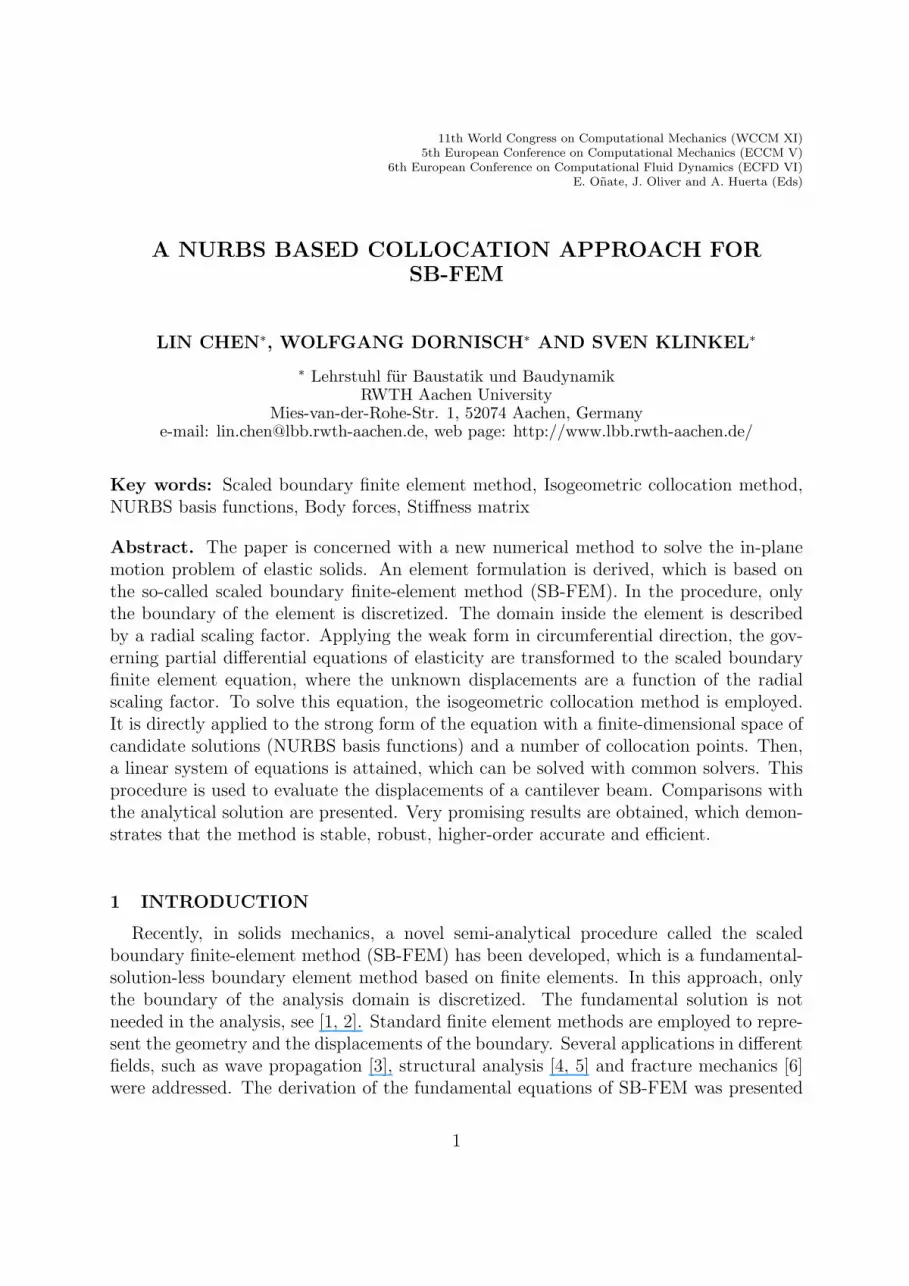
where D is the elasticity matrix. Any general anisotropic material can be used. Forexample, the elasticity matrix of a plane stress linear isotropic material is:

D =E

1− ν2

1 ν 0ν 1 00 0 (1− ν)/2

(4)

The matrices B1 (η) and B2 (η) in the integrand can be obtained as shown in [12] by

B1 (η) =1

|J(η)|b1 (η)N (η) B2 (η) =1

|J(η)|b2 (η)N (η) ,η (5)

in which N (η) is any general shape functions matrix. In the present study it is expressedby

N (η) =

[(1− η)/2 0 (1 + η)/2 0

0 (1− η)/2 0 (1 + η)/2

]. (6)

In Eqs. (3) and (5), |J (η)| is the determination of the Jacob matrix J (η), which is definedby

J (η) =

[x− x0 y − y0x,η y,η

], (7)

where (x, y) are the coordinates of the point on the sub-element AB, which is approxi-mated by the standard finite element method yielding(

xy

)= N (η) (xA, yA, xB, yB)

T . (8)

The coordinate of points inside the shaded triangular area OAB (Fig.2a) are obtained by(xy

)=

(x0

y0

)+ ξ

(N (η) (xA, yA, xB, yB)

T −(

x0

y0

)). (9)

The matrices b1 (η) and b2 (η) in Eq. (5) read

b1(η)T =

[y,η 0 −x,η0 −x,η y,η

]b2(η)

T =

[−y 0 x0 x −y

]. (10)

As the integrations over the sub-element AB are regular, the standard numerical tech-niques in the finite element method, such as Gauss-Legendre quadrature method, aredirectly applicable in Eq. (1).The vector F (ξ) in Eq. (1) is the contribution from the body forces and tractions [13]

F (ξ) = ξ2Fb (ξ) + ξFt (ξ) , (11)

where Fb (ξ) is the contribution of the body force p (ξ) with p (ξ) =[px (ξ) py (ξ)

]T.

Ft (ξ) is the contribution of the prescribed surface tractions t (ξ) =[tx (ξ) ty (ξ)

]T. In

5

Lin Chen, Wolfgang Dornisch and Sven Klinkel

order to obtain F (ξ), akin to the calculation of K11, the corresponding vector of eachsub-element should be calculated firstly, and then assembled. The stress-displacementrelationships reads

σ (ξ, η) = D

(B1 (η) U (ξ) ,ξ +

1

ξB2 (η) U (ξ)

), (12)

see [12]. Here, B1 (η) and B2 (η) are assembled matrices of all sub-elements on the bound-ary Se. According to [13] the internal nodal forces on the inner boundary Si (constant ξ)are equal to

q (ξ) = ξK11U (ξ) ,ξ +K12U (ξ) (13)

where q (ξ) =q1 (ξ) q2 (ξ) . . . qm−1 (ξ) qm (ξ)

Tdenotes the internal nodal forces

of the inner boundary Si (Fig.2a) and qi (ξ) (i = 1, 2, ....,m) are the internal forces of node

i with qi (ξ) =

qix (ξ) qiy (ξ)T

with m being the number of nodes on the boundarySi.For the nodal forces R on the boundary Se of the element ℜ (ξ = 1), it holds R =q (ξ = 1). The stiffness matrix K of the element ℜ relating the nodal forces R and nodaldisplacements U on the boundary Se of the element (ξ = 1) is defined as

R = q (ξ = 1) = KU (ξ = 1)−RF , (14)

whereRF denotes the nodal forces due to body forces and surface tractions of the element.

3 Solution procedure for the scaled boundary finite element equation

The present common solution procedure for the scaled boundary finite element equa-tion (SB-FEE) is based on the eigenvalue method [8] and the matrix function solution [4].However, there are some restrictions existing in both approaches. Thus, in the presentstudy, the isogeometric collocation method is employed to solve the SB-FEE, which is in-troduced in Ref. [11] to solve differential equations. It has been proved to be numericallystable [11]. In isogeometric analysis, both the geometry and the unknown variables arediscretized with the same basis functions. Here Non-uniform Rational B-Splines (NURBS)are used. NURBS are smooth approximating functions constructed by piecewise polyno-mials. To define such functions, a knot vector as a set of non-decreasing real numbersrepresenting coordinates in the parametric space is introduced

Ξ = ξ1 = 0, ...., ξn+p+1 = 1 (15)

where p denotes the order of NURBS and n is the number of basis functions (and controlpoints). For the present study one knot span with p-refinement is used. This has inher-ently benefits for the isogeometric collocation method due to the radial coordinate beingdefined in 0 ≤ ξ ≤ 1. Thus, coordinate transformation is not necessary. The analysis candirectly be carried out with the radial coordinate ξ, which means the radial coordinate ξ

6

Lin Chen, Wolfgang Dornisch and Sven Klinkel

represents the parametric space in the isogeometric analysis. The knot values ξ = 0 andξ = 1 denote the scaling center O and the boundary Se of the element ℜ.In order to construct the NURBS basis functions, B-splines basis function are computedwith the Cox–De Boor formula

p = 0 : Ni,0 (ξ) =

1 if ξi ≤ ξ ≤ ξi+1

0 otherwise

p > 0 : Ni,p (ξ) =ξ − ξi

ξi+p − ξiNi,p−1 (ξ) +

ξi+p+1 − ξ

ξi+p+1 − ξi+1

Ni+1,p−1 (ξ) ,

(16)

in which the specific convention 0/0 = 0 is introduced. Then, the NURBS basis functionsof order p are defined as

Ri,p (ξ) =Ni,p (ξ)ωi∑nj=1Nj,p (ξ)ωj

, (17)

where ωi(i = 1, 2, ...., n) denotes the weight of the i− th basis functions. Obviously, whenall the weights of the NURBS basis functions are equal, the NURBS basis functions willreduce to the B-splines basis functions. Therefore, B-splines are a special case of NURBS.The kth derivative with respect to ξ is given as

dk

dξkRi,p (ξ) =

p

ξi+p − ξi

(dk−1

dξk−1Ri,p−1 (ξ)

)− p

ξi+p+1 − ξi+1

(dk−1

dξk−1Ri+1,p−1 (ξ)

). (18)

Within an isogeometric framework, the radial coordinate ξ and the displacement U (ξ) inthe element ℜ are approximated by NURBS basis functions as

ξ =n∑

i=1

Ri,p (ξ) ξi U(ξ)h =∑n

i=1Ri,p (ξ) U

(ξi)c, (19)

where U(ξi)c

(i = 1, 2, ...., n) are the unknown control variables; ξi are the coordinates ofthe control points, which are obtained by the Greville abscissae due to the specificity ofthe present analysis (1D case with p-refinement):

ξi =ξi+1 + ξi+2 + ....+ ξi+p

p(i = 1, 2, ...., n) (20)

Due to the property of the p-refinement, ξ1 = 0 and ξn = 1 holds.With these approximations, SB-FEE (Eq.(1)) is collocated at the images of the Grevilleabscissae ξi excluding the force boundary of the element ℜ. This can be formally startedby employing Eq.(1), (13) and (14):

ξ2iK11U(ξi),hξξ +ξi (K12 −K21 +K11) U

(ξi),hξ −K22U

(ξi)h

+ F(ξi)= 0 (i = 1, 2, ...., n− 1) (21)

ξnK11U(ξn),hξ +K12U

(ξn)h

= R (22)

7

Lin Chen, Wolfgang Dornisch and Sven Klinkel

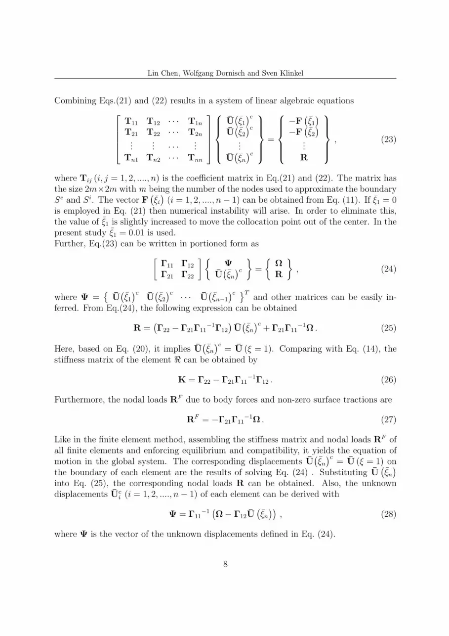
Combining Eqs.(21) and (22) results in a system of linear algebraic equationsT11 T12 · · · T1n

T21 T22 · · · T2n...

... · · · ...Tn1 Tn2 · · · Tnn

U(ξ1)c

U(ξ2)c

...U(ξn)c

=

−F

(ξ1)

−F(ξ2)

...R

, (23)

where Tij (i, j = 1, 2, ...., n) is the coefficient matrix in Eq.(21) and (22). The matrix hasthe size 2m×2m with m being the number of the nodes used to approximate the boundarySe and Si. The vector F

(ξi)(i = 1, 2, ...., n− 1) can be obtained from Eq. (11). If ξ1 = 0

is employed in Eq. (21) then numerical instability will arise. In order to eliminate this,the value of ξ1 is slightly increased to move the collocation point out of the center. In thepresent study ξ1 = 0.01 is used.Further, Eq.(23) can be written in portioned form as[

Γ11 Γ12

Γ21 Γ22

]Ψ

U(ξn)c

=

ΩR

, (24)

where Ψ =

U(ξ1)c

U(ξ2)c · · · U

(ξn−1

)c Tand other matrices can be easily in-

ferred. From Eq.(24), the following expression can be obtained

R =(Γ22 − Γ21Γ11

−1Γ12

)U(ξn)c

+ Γ21Γ11−1Ω . (25)

Here, based on Eq. (20), it implies U(ξn)c

= U (ξ = 1). Comparing with Eq. (14), thestiffness matrix of the element ℜ can be obtained by

K = Γ22 − Γ21Γ11−1Γ12 . (26)

Furthermore, the nodal loads RF due to body forces and non-zero surface tractions are

RF = −Γ21Γ11−1Ω . (27)

Like in the finite element method, assembling the stiffness matrix and nodal loads RF ofall finite elements and enforcing equilibrium and compatibility, it yields the equation ofmotion in the global system. The corresponding displacements U

(ξn)c

= U (ξ = 1) onthe boundary of each element are the results of solving Eq. (24) . Substituting U

(ξn)

into Eq. (25), the corresponding nodal loads R can be obtained. Also, the unknowndisplacements Uc

i (i = 1, 2, ...., n− 1) of each element can be derived with

Ψ = Γ11−1

(Ω− Γ12U

(ξn))

, (28)

where Ψ is the vector of the unknown displacements defined in Eq. (24).

8

Lin Chen, Wolfgang Dornisch and Sven Klinkel

Substituting U(ξn)and Eq. (28) into (19), the displacement U (ξ) of each element can

be obtained. The displacement U (ξ, η) inside each element can be calculated as [13]:

U (ξ, η) = N (η) U (ξ) (29)

The stress σ (ξ, η) inside each element can be obtained by substituting Eq. (19) intoEq. (12). Here, the displacement U (ξ, η) and stress σ (ξ, η) are defined in the localcoordinate system (ξ, η). The corresponding values in the global coordinate system (x, y)are obtained by the coordinate transformation from Eq. (9).

10

3

1000P

1000P

x

y

A

BE

F

Figure 3: Cantilever beam under pure bending moment

0

0.5

1

1.5

2

2.5

3

3.5

4

4.5

5

0 10 20 30 40 50 60

Ver

tica

l D

isp

lace

men

t

Total Number of Dof

1 Elem

2 Elem

4 Elem

8 Elem

16 Elem

FEM

Figure 4: Vertical displacement at point A of the cantilever beam

4 Numerical example

In order to verify the theory, calculations were performed for a cantilever beam (Fig.3).Pure bending moment M = 3P is exerted at the end of the beam. The properties of thebeam are: Young’s modulus E = 15000, thickness d = 1 and Poisson’s ratio µ = 0.0. Fig.3shows the diagram in which the vertical displacement vA at point A is plotted versus thetotal number of degree-of-freedom in the calculation. In the analysis, the beam is equally

9

Lin Chen, Wolfgang Dornisch and Sven Klinkel

discretized by rectangular elements along x-direction. In y-direction, one element throughthe thickness is employed. The total number of nodes, employed in the discretization, is4, 6, 10, 18 and 34 nodes, respectively, which are uniformly distributed at the boundaryAF and BE. For example, if 4 nodes are employed, there are 2 nodes on the boundary AFand BE separately. For such amount of nodes, the maximum number of elements is 16with 4 nodes per element. Since there is no restriction of the number of nodes per elementin the proposed approach, we examined one element with different number of nodes. Forexample, when the beam is only modeled by one element, there could be with 4, 6, 10,18 and 34 nodes on the element. Analogously, if the beam is discretized by 2 elements,the number of nodes per element could be 4, 6, 10 and 18 nodes, correspondingly. Also,for better illustration, comparison with standard finite element method (FEM) with the4-node quadrilateral plane element (linear shape functions) is made. In FEM, the beamis only discretized along x-direction. In y-direction, only one element is used throughthe height. Thus, we could have 1, 2, 4, 8 and 16 elements with 4, 6, 10, 18 and 34nodes, respectively. The results of the proposed method converge to the exact solutionwith increasing number of elements and nodes (See Fig.4). In general, the solutions ofstandard finite element method (FEM) are less accurate compared to those of the proposedapproach. One could have results almost identical to those of FEM by discretizing thebeam with one element in the present study.

0

1

2

3

A

B

0

1

2

3

A

B

O

(a) 16 elements (b) 15 major elements plus 10 sub-elements

Figure 5: Dicretization of the beam

Next, in order to illustrate the proficiency of the proposed approach, the cantilever beamin Fig.3 is employed. The beam is firstly divided by 8 elements with 4-node quadrilateralplane elements (See Fig.5a), which is termed as ’initial mesh’. For such discretization, thedisplacement at the boundary AB is linear. However, the real displacement distribution atAB is non-linear. To represent it, the beam is further discretized by several quadrilateralplane sub-elements (See Fig.5b), which is termed as ’re-mesh’. The deflection of boundaryAB with respect to the neutral point O is shown in Fig.6. It can be observed that theboundary AB is non-linearly deflected, which implies that the proposed approach caneasily obtain more accurate solutions by refining one element with many sub-elementswithout adding new calculation effort. It is worth noting that such ability of elementrefinement allows local refinement at concentration problem in solids mechanics. Also, itis interesting to note that the standard finite element method (FEM) cannot deal with

10

Lin Chen, Wolfgang Dornisch and Sven Klinkel

-1.5

-1

-0.5

0

0.5

1

1.5

-0.3 -0.2 -0.1 0 0.1 0.2 0.3

Hei

gh

t

Deflection

Re-mesh

Initial Mesh

Figure 6: Deflection of boundary AB

this type of discretization in Fig.5b.

5 Conclusions

In this paper, a new numerical method is proposed to solve the in-plane motion prob-lem of elastic solids. A novel element formulation is derived, which is based on the scaledboundary finite element method (SB-FEM) and isogeometric collocation method. In theprocedure, the analysis domain is discretized to finite elements. The calculation is firstlyperformed to obtain the stiffness matrix of each element and the nodal forces due to bodyforces. In the implementation, SB-FEM is employed to transform the governing partialdifferential equations of elasticity to the so-called scaled boundary finite element equation,which is a non-homogenous ordinary differential equation of Euler type for the displace-ments. In order to solve it, the isogeometric collocation method is employed. The SB-FEequation is evaluated at all collocation points, assembled to a system of linear algebraicequations and solved. Displacements and stresses can be computed. The numerical exam-ples demonstrate, that the procedure is stable, robust, higher-order accurate and efficient.Further applications of this approach can be extended to trimmed-NURBS, because theboundary-oriented character of SB-FEM ideally corresponds to the trimming of elementswith NURBS curves, which is the way trimmed-NURBS surfaces are described.

Acknowledgements

The financial support of the Siemens AG and DAAD (German Academic ExchangeService) for the research is gratefully acknowledged.

11

Lin Chen, Wolfgang Dornisch and Sven Klinkel

References

[1] C. Song, J. P. Wolf, The scaled boundary finite-element method-alias consistentinfinitesim.al finite-element cell method-for elastodynamics, Comput. Methods Appl.Mech. Engrg. 147 (1997) 329–355.

[2] J. P. Wolf, C. Song, The scaled boundary finite-element method - a fundamentalsolution-less boundary-element method, Comput. Methods Appl. Mech. Engrg. 190(2001) 5551–5568.

[3] H. Gravenkamp, F. Bause, C. Song, On the computation of dispersion curves foraxisymmetric elastic waveguides using the scaled boundary finite element method,Comput. Struct. 131 (2014) 46–55.

[4] C. Song, A matrix function solution for the scaled boundary finite-element equationin statics, Comput. Methods Appl. Mech. Engrg. 193 (2004) 2325–2356.

[5] G. Lin, Y. Zhang, Z. Hu, H. Zhong, Scaled boundary isogeometric analysis for 2delastostatics, Science China Physics, Mechanics and Astronomy 57 (2014) 286–300.

[6] S. Goswami, W. Becker, Computation of 3-d stress singularities for multiple cracksand crack intersections by the scaled boundary finite element method, Int. J. Fracture175 (2012) 13–25.

[7] C. Song, J. P. Wolf, The scaled boundary finite-element method: analytical solutionin frequency domain, Comput. Methods Appl. Mech. Engrg. 164 (1998) 249–264.

[8] C. Song, J. P. Wolf, The scaled boundary finite-element method–a primer: solutionprocedures, Comput. Struct. 78 (2000) 211–225.

[9] T. J. R. Hughes, J. A. Cottrell, Y. Bazilevs, Isogeometric analysis: CAD, finiteelements, NURBS, exact geometry and mesh refinement, Comput. Meth. Appl.Mech. Engrg. 194 (2005) 4135–4195.

[10] D. Schillinger, J. A. Evans, A. Reali, M. A. Scott, T. J. Hughes, Isogeometric colloca-tion: Cost comparison with galerkin methods and extension to adaptive hierarchicalnurbs discretizations, Comput. Methods Appl. Mech. Engrg. 267 (2013) 170–232.

[11] F. Auricchio, L. B. Da Veiga, T. Hughes, A. Reali, G. Sangalli, Isogeometric collo-cation methods, Math. Mod. Meth. Appl. S. 20 (2010) 2075–2107.

[12] J. P. Wolf, C. Song, The scaled boundary finite-element method–a primer: deriva-tions, Comput. Struct. 78 (2000) 191–210.

[13] C. Song, J. P. Wolf, Body loads in scaled boundary finite-element method, Comput.Methods Appl. Mech. Engrg. 180 (1999) 117–135.

12