Numerische Mathematik manuscript No.(will be inserted by the editor)

Multiscale RBF collocation for solving PDEs on spheres

Q. T. Le Gia · I. H. Sloan · H. Wendland

Received: date / Accepted: date

Abstract In this paper, we discuss multiscale radial basis function collocation methods forsolving certain elliptic partial differential equations on the unit sphere. The approximatesolution is constructed in a multi-level fashion, each level using compactly supported radialbasis functions of smaller scale on an increasingly fine mesh. Two variants of the collocationmethod are considered (sometimes called symmetric and unsymmetric, although here bothare symmetric). A convergence theory is given, which buildson recent theoretical advancesfor multiscale approximation using compactly supported radial basis functions.

Keywords partial differential equation· multiscale· collocation· unit sphere

Mathematics Subject Classification (2000)65N35· 65N55

1 Introduction

Partial differential equations (PDEs) on the unit sphere have many applications in the geo-sciences. Since analytic solutions are difficult or impossible to find, good algorithms forfinding approximate solutions are essential. Radial basis functions (RBFs) present a simpleand effective way to construct approximate solutions to PDEs on spheres, via a colloca-tion method [16] or a Galerkin method [13]. They have been used successfully for solvingtransport-like equations on the sphere [3,4].

The quality of the approximation depends on the distribution of the centers of the RBFsused to define the approximate solution. However, in practice the solution usually repre-sents some physical quantities, which are available in manyphysical scales. A solution usingRBFs with a single scale may fail to capture these features, unless the radial basis functionhas a large support and the number of centers is also large, a combination which can be com-putationally prohibitive. To overcome this, we propose a multiscale approximation scheme,

Q. T. Le GiaSchool of Mathematics and Statistics, University of New South Wales, Sydney, NSW 2052, Australia.

I. H.SloanSchool of Mathematics and Statistics, University of New South Wales, Sydney, NSW 2052, Australia.

H. WendlandMathematical Institute, University of Oxford, 24-29 St Giles’ Oxford, OX1 3LB England.

2

in which the approximate solution is constructed using a multi-stage process, in which theresidual of the current stage is the target function for the next stage, and in each stage, RBFswith smaller support and with more closely spaced centers will be used as basis functions.

While meshless methods using RBFs have been employed to derive numerical solutionsfor PDEs on the sphere only recently [16,13,3,4], it should be mentioned that approxima-tion methods using RBFs for PDEs on bounded domains have beenaround for the last twodecades. Originally proposed by Kansa [11,12] for fluid dynamics, approximation methodsfor many types of PDEs defined on bounded domains inR

n using RBFs have since beenused widely. Examples include [1,6,9,10].

For boundary value problems, the technique predominantly used in the literature, withthe exception of [23], where a Galerkin method was used, has been collocation, mainly be-cause of the simplicity and the fact that there is no requirement for numerical integration,which is still a problematic issue in all meshfree methods. There are two popular approachesto deriving the approximation scheme, usually called unsymmetric and symmetric colloca-tion. In the first approach the collocation matrix is unsymmetric on bounded domains be-cause of the two different operators involved, the differential operator and the boundaryoperator. This however can lead to nonsolvable systems [10]. Nonetheless, the method iswidely used since the solution is just a linear combination of the RBFs and usually showsgood approximation properties. In our case, where our differential operator is independentof position and we do not have a boundary, the nonsymmetric approach turns out actuallyto be an alternative symmetric approach, which we will referto as thestandard collocationmethod.

In the classical symmetric approach the operators are incorporated into the approxima-tion space and hence the collocation matrix is symmetric andalways positive definite, butthe numerical solution is slightly more complicated to construct. Since the solution mini-mizes a certain Hilbert space norm amongst all possible functions satisfying the collocationcondition, we will refer to this approach asnorm-minimal collocation. A comparison of thetwo variants can be found in [19].

A common drawback of using RBFs in approximation schemes forPDEs is that the col-location matrix arising from the approximation problem tends to be ill-conditioned. Thereare two main approaches to overcome this: either to use a preconditioner, or to use a multi-level approximation approach. With a multilevel method, the condition number of the matrixat each level can be relatively small, and has only slow growth. There are papers [1,2] deal-ing with multilevel approximation methods for PDEs using compactly supported radial basisfunctions on bounded domains inRn, however the theory there is incomplete. In this work,we will prove convergence results in Sobolev spaces for bothkinds of collocation for a classof elliptic PDEs defined on the unit sphereS

n ⊂ Rn+1.

The present paper builds upon theoretical advances in multiscale approximation for thesphere [15], which were subsequently extended to bounded regions inR

n [25].

In Section 2 we will review necessary background on spherical harmonics, positive defi-nite kernels, and Sobolev spaces on the unit sphere. In Section 3 we will present two variantsof the collocation method for solving PDEs on the unit sphereusing RBFs of a single scale.In Section 4 we present the corresponding multiscale methods. A convergence theorem forthe multiscale methods will be proved. Finally, Section 5 presents some numerical examples.

3

2 Preliminaries

In our work, we will use zonal functions to construct approximate solutions for the PDEs.Zonal functions onSn are functions that can be represented asφ(x · y) for all x,y ∈ S

n,whereφ(t) is a continuous function on[−1,1]. We shall be concerned exclusively withzonal kernels of the type

Φ(x,y) = φ(x ·y) =∞

∑ℓ=0

aℓPℓ(n+1;x ·y), aℓ > 0,∞

∑ℓ=0

aℓ < ∞, (1)

where{Pℓ(n+1;t)}∞ℓ=0 is the sequence of(n+1)-dimensional Legendre polynomials nor-

malized toPℓ(n+ 1;1) = 1. Thanks to the seminal work of Schoenberg [22] and the laterwork of [26], we know that such aφ is (strictly) positive definite onSn, that is, the matrixA := [φ(xi · x j)]

Mi, j=1 is positive definite for every set of distinct points{x1, . . . ,xM} on S

n

and every positive integerM.For mathematical analysis it is sometimes convenient to expand the kernelΦ(x,y) into

a series of spherical harmonics. A detailed discussion on spherical harmonics can be foundin [17]. In brief, spherical harmonics are the restriction to S

n of homogeneous polynomialsY(x) in R

n+1 which satisfy∆Y(x) = 0, where∆ is the Laplacian operator inRn+1. Thespace of all spherical harmonics of degreeℓ on S

n, denoted byHℓ, has anL2 orthonormalbasis

{Yℓk : k = 1, . . . ,N(n, ℓ)},

where

N(n,0) = 1 andN(n, ℓ) =(2ℓ+n−1)Γ (ℓ+n−1)

Γ (ℓ+1)Γ (n)for ℓ ≥ 1,

thus ∫

SnYℓkYℓ′k′dS= δℓℓ′δkk′ ,

wheredS is the surface measure of the unit sphere. The space of spherical harmonics ofdegree≤ L will be denoted byPL :=

⊕Lℓ=0Hℓ; it has dimensionN(n+1,L). Every function

g∈ L2(Sn) can be expanded in terms of spherical harmonics,

g =∞

∑ℓ=0

N(n,ℓ)

∑k=1

gℓkYℓk, gℓk =∫

SngYℓkdS.

Using the addition theorem for spherical harmonics (see, for example, [17, page 10]),

N(n,ℓ)

∑k=1

Yℓk(x)Yℓk(y) =N(n, ℓ)

ωnPℓ(n+1;x ·y), (2)

we can write

Φ(x,y) =∞

∑ℓ=0

N(n,ℓ)

∑k=1

φ(ℓ)Yℓk(x)Yℓk(y), whereφ(ℓ) =ωn

N(n, ℓ)aℓ, (3)

whereωn is the surface area ofSn. We shall assume that, for someσ > n/2,

c1(1+ ℓ)−2σ ≤ φ(ℓ) ≤ c2(1+ ℓ)−2σ , ℓ ≥ 0. (4)

4

In the remainder of the paper, we usec1,c2, . . . to denote specific constants whilec,c′,C aregeneric constants, which may take different values at each occurrence.

Assume that we are given a positive definite kernel onSn defined from a compactly

supported radial basis functionR : Rn+1 → R

Φ(x,y) = R(x−y) = ρ(|x−y|), x,y ∈ Sn,

where| · | is the Euclidean distance inRn+1. We may then define a scaled version,

Φδ (x,y) =1

δ n R

(x−y

δ

), x,y ∈ S

n, (5)

whereδ > 0 is a scaling parameter. In the following, we expandΦδ as

Φδ (x,y) =∞

∑ℓ=0

N(n,ℓ)

∑k=1

φδ (ℓ)Yℓk(x)Yℓk(y), x,y ∈ Sn. (6)

We assume, strengthening (4), that for someσ > n/2,

c1(1+δℓ)−2σ ≤ φδ (ℓ) ≤ c2(1+δℓ)−2σ , ℓ ≥ 0. (7)

In fact, we have shown previously ([15, Theorem 6.2]) that condition (7) is satisfied ifR isa compactly supported RBF of Wendland’s type [24].

Thenative spaceassociated withΦ is defined to be

NΦ =

{g∈ D

′(Sn) : ‖g‖2Φ =

∞

∑ℓ=0

N(n,ℓ)

∑k=1

|gℓk|2

φ(ℓ)< ∞

},

whereD ′(Sn) is the space of distributions onSn. More details on native spaces can be foundin [24]. It can be shown thatNΦ is a Hilbert space with respect to the following innerproduct

〈 f ,g〉Φ =∞

∑ℓ=0

N(n,ℓ)

∑k=1

fℓkgℓk

φ(ℓ), f ,g∈ NΦ .

Moreover, we can show thatΦ is a reproducing kernel forNΦ , i.e. for allg∈ NΦ ,

〈g(·),Φ(x, ·)〉Φ = g(x), x ∈ Sn. (8)

The Sobolev spaceHσ = Hσ (Sn) with real parameterσ is defined by

Hσ (Sn) :=

{g∈ D

′(Sn) : ‖g‖2Hσ :=

∞

∑ℓ=0

N(n,ℓ)

∑k=1

(1+ ℓ)2σ |gℓk|2 < ∞

}.

Under the conditionσ > n/2, the norms‖ · ‖Φ and‖ · ‖Hσ are equivalent if (4) holds, withthe norms related by

c1/21 ‖g‖Φ ≤ ‖g‖Hσ ≤ c1/2

2 ‖g‖Φ . (9)

Using the scaled version of the kernelΦδ (x,y), for a functiong ∈ NΦ we define thefollowing norm:

‖g‖Φδ :=

(∞

∑ℓ=0

N(n,ℓ)

∑k=1

|gℓk|2

φδ (ℓ)

)1/2

. (10)

This norm, too, is equivalent to the norm‖g‖Hσ . The following lemma gives informationabout that equivalence.

5

Lemma 1 For σ > n/2 andδ ≤ 2, for all g∈ Hσ (Sn), we have

2−σ c1/21 ‖g‖Φδ ≤ ‖g‖Hσ ≤ 2σ δ−σ c1/2

2 ‖g‖Φδ .

Proof. This is essentially Lemma 3.1 in [15]. ⊓⊔

3 Single-scale Collocation for Solving PDEs

We consider the following PDE

Lu = f on Sn, (11)

whereL is an elliptic self-adjoint differential operator with constant symbolL(ℓ) and ordert, for somet > 0. That is, we can expandLu as a Fourier series

Lu =∞

∑ℓ=0

N(n,ℓ)

∑k=1

L(ℓ)uℓkYℓk

in which

c3(1+ ℓ)t ≤ L(ℓ) ≤ c4(1+ ℓ)t , ℓ ≥ 0, (12)

wherec3,c4 are two positive constants independent ofℓ. For example, we may takeL =−∆ ∗ + ω2, where∆ ∗ is the Laplace–Beltrami operator andω > 0, in which caseL(ℓ) =ℓ(ℓ+n−1)+ω2 andt = 2.

SinceL(ℓ) > 0 for ℓ ≥ 0, we can defineL1/2 by

L1/2u =∞

∑ℓ=0

N(n,ℓ)

∑k=1

√L(ℓ)uℓkYℓk.

Note that we have an intrinsic relation between the smoothness of the given functionfand the solutionu of (11), as follows:f ∈ Hσ if and only if u∈ Hσ+t . Hence, in the futurewe can make assumptions on the smoothness of the solutionu, which translate immediatelyto assumptions onf .

In this section, we will discuss collocation methods to solve (11) approximately. Initially,our collocation methods will be based upon radial basis functions of a single scale. We willdiscuss two single scale approaches, known in the literature as symmetric and unsymmetriccollocation.

SupposeX := {x1, . . . ,xN} ⊆ Sn is a given discrete set of scattered points on then-

dimensional sphereSn. Then solving equation (11) by collocation on the setX means to finda functionuh from a given approximation space which satisfies the collocation equations

Luh(x j) = Lu(x j) = f (x j), 1≤ j ≤ N. (13)

6

3.1 Standard Collocation

When working with radial basis functions, an obvious approach to finding such an approxi-mate solution is as follows.

Suppose thatΦ is a kernel that satisfies condition (4) for someσ > (t + n)/2. Thisassumption guarantees that we may applyL to one of the arguments ofΦ and still havea continuous function. Hence, we may pick our approximationuh from the approximationspace

VX := span{Φ(·,x j) : x j ∈ X}. (14)

To finduh ∈VX, we representuh as a linear combination of the basis functions inVX:

uh =N

∑j=1

b jΦ(·,x j),

and the condition (13) leads now to the linear system

Ab = f, (15)

whereA is the collocation matrix with entriesai, j = LΦ(xi ,x j) and the right-hand side isgiven byf = ( f (x j)).

Here, the functionLΦ is defined to be the kernel having the Fourier expansion

LΦ(x,y) =∞

∑ℓ=0

N(n,ℓ)

∑k=1

φ(ℓ)L(ℓ)Yℓk(x)Yℓk(y), (16)

which can be computed by applyingL to either of the arguments ofΦ . In particular, thenew kernelLΦ is symmetric and positive definite, since its Fourier coefficientsL(ℓ)φ(ℓ) arepositive. This ensures that the system (15) is always uniquely solvable.

Lemma 2 Letσ > (t +n)/2 and assume thatΦ satisfies(4) and VX is given by(14). Thereexists a unique function uh ∈VX satisfying the collocation conditions (13). The solution uh

belongs to Hσ+t/2.

Proof. Existence and uniqueness have been established already. The second part followsfrom the fact that eachϕ j := Φ(·,x j) belongs toHσ+t/2. To see this, we note from (3) thatϕ j(ℓ) = φ(ℓ)Yℓk(x j), which leads via (4) to

‖ϕ j‖2Hσ+t/2 =

∞

∑ℓ=0

N(n,ℓ)

∑k=1

φ(ℓ)2Yℓk(x j)2(1+ ℓ)2σ+t

≤ c22

∞

∑ℓ=0

N(n,ℓ)

∑k=1

Yℓk(x j)2(1+ ℓ)t−2σ

= c22

∞

∑ℓ=0

N(n, ℓ)

ωnPℓ(n+1;1)(1+ ℓ)t−2σ

≤ c∞

∑ℓ=0

(1+ ℓ)t−2σ+n−1,

where we have used the addition theorem (2), the fact that theLegendre polynomials are nor-malized toPℓ(n+1;1) = 1, and the fact that the dimensionN(n, ℓ) behaves like(1+ ℓ)n−1.This sum is finite ift −2σ +n−1 < −1 which is equivalent to our assumption onσ . ⊓⊔

7

This result stands in sharp contrast to standard RBF collocation for boundary valueproblems. In the situation of solving a PDE on a bounded domain with given boundaryvalues, this approach does not always lead to an invertible collocation matrix, see [10].Nonetheless, it is widely used, usually under the nameunsymmetric collocation.

To understand the solution process, we introduce a new kernel Ψ defined by

Ψ = L−1Φ .

This kernel has Fourier coefficientsψ(ℓ) = φ(ℓ)/L(ℓ) and hence defines an inner product〈·, ·〉Ψ ,

〈 f ,g〉Ψ =∞

∑ℓ=0

N(n,ℓ)

∑k=1

L(ℓ) fℓkgℓk

φ(ℓ), f ,g∈ Hσ+t/2, (17)

and the corresponding norm by‖g‖2Ψ = 〈g,g〉Ψ . Under our assumptions (4) and (12) on the

kernelΦ and the operatorL, respectively, we easily see that the‖ · ‖Ψ norm is equivalent tothe Sobolev norm‖ · ‖Hσ+t/2, and thatHσ+t/2 with the inner product (17) is a reproducingkernel Hilbert space with kernelΨ . As in the case of the original kernelΦ , we can define ascaled version ofΨ , that is

Ψδ := L−1Φδ .

This kernel defines an inner product〈·, ·〉Ψδ, which is defined by

〈 f ,g〉Ψδ=

∞

∑ℓ=0

N(n,ℓ)

∑k=1

L(ℓ) fℓkgℓk

φδ (ℓ), f ,g∈ Hσ+t/2, (18)

and the corresponding norm is‖g‖Ψδ =√〈g,g〉Ψδ

. This norm is also equivalent to the

Sobolev norm‖ · ‖Hσ+t/2, as given in the following lemma.

Lemma 3 For σ > n/2 andδ ≤ 2, for all g∈ Hσ+t/2(Sn), we have

c5‖g‖Ψδ ≤ ‖g‖Hσ+t/2 ≤ c6δ−σ‖g‖Ψδ .

Proof. Sinceδ ≤ 2, using (7), (12) and (18) we have

‖g‖2Ψδ

=∞

∑ℓ=0

N(n,ℓ)

∑k=1

L(ℓ)|gℓk|2

φδ (ℓ)

≤ c4

c1

∞

∑ℓ=0

N(n,ℓ)

∑k=1

(1+ ℓ)t |gℓk|2(1+δℓ)2σ

≤ 22σ c4

c1

∞

∑ℓ=0

N(n,ℓ)

∑k=1

|gℓk|2(1+ ℓ)2σ+t =22σ c4

c1‖g‖2

Hσ+t/2.

We also have(1+δℓ) = δ (1/δ + ℓ) ≥ δ (1/2+ ℓ/2). Hence,

(1+ ℓ)2σ ≤ 22σ δ−2σ (1+δℓ)2σ ,

and again using (7) and (18),

‖g‖2Hσ+t/2 =

∞

∑ℓ=0

N(n,ℓ)

∑k=1

|gℓk|2(1+ ℓ)2σ+t

≤ 22σ δ−2σ∞

∑ℓ=0

N(n,ℓ)

∑k=1

(1+ ℓ)t |gℓk|2(1+δℓ)2σ ≤ 22σ δ−2σ c2c−13 ‖g‖2

Ψδ.

Settingc5 := (c1/c4)1/22−σ andc6 := 2σ (c2/c3)

1/2 we obtain the result of the lemma.⊓⊔

8

Lemma 4 Let u∈ Hσ+t/2 with σ > (t +n)/2. Let uh ∈VX be the solution of the collocationequation(13)by the standard approach. Then

〈u−uh,χ〉Ψ = 0 for all χ ∈VX, (19)

and hence‖u−uh‖Ψ ≤ ‖u‖Ψ . (20)

Proof. From the collocation equation (13) we haveLu(x j) = Luh(x j) for all x j ∈ X. Thismeans that the error functioneh = u− uh satisfiesLeh(x j) = 0 for all x j ∈ X, and hence,sinceL is invertible and self-adjoint,

⟨eh,Φ(·,x j)

⟩Ψ =

⟨Leh,L

−1Φ(·,x j)⟩

Ψ

=⟨Leh,Ψ(·,x j)

⟩Ψ

= Leh(x j) = 0.

SinceVX is the finite dimensional space spanned byΦ(·,x j) we obtain (19), which immedi-ately implies Pythagoras’ theorem,

‖u−uh‖2Ψ +‖uh‖2

Ψ = ‖u‖2Ψ ,

from which inequality (20) follows. ⊓⊔We will now discuss the erroru−uh. As usual, we will use the mesh normhX, which is

defined byhX := sup

x∈Snminx j∈X

θ(x,x j),

whereθ(x,y) = cos−1(x ·y) is the geodesic distance betweenx andy.

Theorem 1 Assume that the exact solution u belongs to Hσ+t/2 with σ > (t +n)/2. Let hX

be the mesh norm of the scattered set X, letΦ be a positive definite kernel satisfying(4) andlet uh ∈VX be the approximate solution obtained by the collocation equation (13). Then,

‖u−uh‖L2 ≤ c‖L1/2(u−uh)‖L2 ≤ chσ−t/2X ‖u−uh‖Hσ+t/2 ≤ chσ−t/2

X ‖u‖Hσ+t/2.

Proof. Since the functionLu− Luh vanishes onX and belongs toHσ−t/2, the “samplinginequality”, [14, Theorem 3.3], guarantees the existence of a constantc > 0 such that

‖Lu−Luh‖L2 ≤ chσ−t/2X ‖Lu−Luh‖Hσ−t/2 ≤ chσ−t/2

X ‖u−uh‖Hσ+t/2,

where, in the last step, we have used the condition (12) and the definition of Sobolev norms.Using (12) again and the equivalence between the‖ · ‖Ψ norm and the norm‖ · ‖Hσ+t/2, weobtain

‖u−uh‖L2 ≤ c‖L1/2(u−uh)‖L2

≤ c‖Lu−Luh‖L2

≤ chσ−t/2X ‖u−uh‖Hσ+t/2

≤ chσ−t/2X ‖u−uh‖Ψ

≤ chσ−t/2X ‖u‖Ψ

≤ chσ−t/2X ‖u‖Hσ+t/2,

where we used Lemma 4 in the last but one step. ⊓⊔

9

3.2 Norm-minimal Collocation

We will now discuss another collocation technique. Assume that we know that the exactsolutionu belongs toHσ and assume thatΦ is a reproducing kernel ofHσ in the sense thatits Fourier coefficients satisfy (4). Then, it seems naturalto choose an approximate solutionuh as the solution of

min{‖s‖Φ : s∈ Hσ with Ls(x j) = f (x j), 1≤ j ≤ N

}, (21)

i.e.,uh is minimizing the native space norm amongst all possible functions that collocate thegiven data. It turns out that this corresponds to what is known as thesymmetric collocationmethod, see [24]. However, we have now to assume thatσ > t +n/2.

It can be shown, in a much more general context, that the solution of (21) must neces-sarily come from the finite dimensional space

WX := span{LΦ(·,x j) : 1≤ j ≤ N},

and that the concrete solutionuh ∈WX can be computed by imposing the collocation condi-tions (13). To finduh, we can representuh as a linear combination of the basis functions inWX:

uh =N

∑j=1

b jLΦ(·,x j)

and condition (13) will then lead to the linear system

Ab = f, (22)

whereA is now the collocation matrix with entriesai j = LLΦ(xi ,x j) and the right-hand sideis again given byf = ( f (x j)).

It is also well-known that this symmetric collocation solution is the best approximationfrom WX in the native space norm, see [24].

Lemma 5 Suppose u∈ Hσ with σ > t +n/2 is the exact solution of(11). Let uh ∈WX bethe solution of (21). Then,

〈u−uh,χ〉Φ = 0 for all χ ∈WX, (23)

and hence‖u−uh‖Φ ≤ ‖u‖Φ . (24)

Proof. For j = 1, . . . ,N we have, using the reproducing property ofΦ and the self-adjointproperty ofL,

⟨u−uh,LΦ(·,x j)

⟩Φ =

⟨L(u−uh),Φ(·,x j)

⟩Φ

= Lu(x j)−Luh(x j) = 0,

from which the result follows immediately. ⊓⊔Error estimates for the norm-minimal collocation method have, even in the more com-

plicated situation of bounded domains, been derived in [5,8].The error between the solution and the approximate solutiondepends on the mesh norm

hX of the setX, as given in the following convergence theorem.

10

Theorem 2 Assume that u∈ Hσ , for σ > t +n/2, is the exact solution of(11)and uh ∈WX

is the solution of (21). Then, provided hX is sufficiently small,

‖u−uh‖L2 ≤ chσ−tX ‖u−uh‖Hσ ≤ chσ−t

X ‖u‖Hσ .

Proof. Since the functionLu− Luh vanishes onX, we can again employ the “samplinginequality” from [14, Theorem 3.3], which gives a constantc > 0 such that

‖Lu−Luh‖L2 ≤ chσ−tX ‖Lu−Luh‖Hσ−t ≤ chσ−t

X ‖u−uh‖Hσ

≤ chσ−tX ‖u−uh‖Φ ,

where in the last two steps we have used condition (12), the definition of Sobolev normsand the equivalence (9). Using condition (12) again and the equivalence between the nativespace norm‖ · ‖Φ and the Sobolev norm‖ · ‖Hσ we obtain

‖u−uh‖L2 ≤ c‖Lu−Luh‖L2 ≤ chσ−tX ‖u−uh‖Φ ≤ chσ−t

X ‖u‖Φ

≤ chσ−t‖u‖Hσ ,

where in the second to last step we have used (24) from Lemma 5. ⊓⊔

3.3 Sharpness of the Results

In both Theorems 1 and 2 we used an inequality of the form

‖u−uh‖L2 ≤ ‖Lu−Luh‖L2.

This clearly is a coarse estimate, which one might think would leave some leeway for betterestimates. Interestingly, the following 1-dimensional example shows that the estimates inTheorems 1 and 2 are the best we can hope for.

Lemma 6 Consider Lu= f on S1 where L is defined byL(ℓ) = (1+ ℓ)t , t > 0. Let X =

{x j = jπ/m : 1≤ j ≤ 2m} and let uh be any collocation solution satisfying Luh(x j) = f (x j).Assume that the collocation solution is constructed from a kernelΦ which satisfies(4) forsomeσ > t/2+1/2 for the standard method, orσ > t +1/2 for the norm-minimal method.Then, for the standard collocation method

supu∈Hσ+t/2

‖u−uh‖L2

‖u‖Hσ+t/2≥Chσ−t/2

X ,

while for the norm-minimal collocation method

supu∈Hσ

‖u−uh‖L2

‖u‖Hσ≥Chσ−t

X .

Proof. Let f (x)= sin2(mx)= 12(1−cos2mx), m∈N, and letk= 2m. The pseudo-differential

operatorL of ordert is defined by its effect on the eigenfunctions,

L(cos(ℓx)) = (1+ ℓ)t cos(ℓx), L(sin(ℓx)) = (1+ ℓ)t sin(ℓx).

Then the pseudo-differential equationLu = f admits the exact solution

u(x) =12

(1− cos(kx)

(1+k)t

).

11

For the chosen collocation points we havef (x j) = 0 and hence the approximate solutionuh

is identically zero. It is easily seen that the mesh norm ofX is hX = π/k. We therefore have

‖u−uh‖2L2

= ‖u‖2L2

=π2

+π

4(1+k)2t ≥π2

.

TheHσ norm ofu can also be computed,

‖u‖2Hσ =

π2

+π4

(1+k)2(σ−t).

For the norm-minimal case we haveσ > t, and hence‖u‖2Hσ ≤ ck2(σ−t), and

‖u−uh‖L2

‖u‖Hσ=

‖u‖L2

‖u‖Hσ≥ ck−(σ−t) = Chσ−t

X .

Similarly, theHσ+t/2 norm ofu can also be computed,

‖u‖2Hσ+t/2 =

π2

+π4

(1+k)2σ−t .

Thus, for the standard collocation case we have (sinceσ > t/2) ‖u‖2Hσ+t/2 ≤ ck2σ−t , and

hence‖u−uh‖L2

‖u‖Hσ+t/2=

‖u‖L2

‖u‖Hσ+t/2≥ ck−(σ−t/2) = Chσ−t/2

X .

⊓⊔

4 Multiscale Collocation for Solving PDEs

While the (fixed) single scale approach for solving PDEs via collocation yields good ap-proximation in both the standard and the norm-minimizing approaches, it suffers from twomajor drawbacks. On the one hand, the condition number growsrapidly with decreasingfill distance. On the other hand, even when using compactly supported RBFs, the matricesquickly become dense, and as a result the computational costbecomes prohibitive.

Recently (see [15,25]), in the case of interpolation, a multiscale technique has beenproven to have the advantages of good approximation and computational efficiency. Weare now going to analyze how this method can be carried over tosolving PDEs. We knowalready from numerical examples that, at least in the boundary value PDE case (see [1]),the approach has to be modified to be successful. The theory below will guide us to anappropriate modification for PDEs on the sphere.

The general idea of the multiscale approach can be describedas follows.We start with a widely spread set of pointsX1 and use a basis function with a large

scaleδ1 to recover the global behavior of the solutionu, by solving the collocation equationLs1|X1 = f |X1. We then setu1 = s1 as the first approximation, so that the residual at the firststep is f1 = f −Ls1. To reduce the residual, at the next step we use a finer set of points X2

and a smaller scaleδ2, and compute a corrections2 from an appropriate finite dimensionalspace by solvingLs2|X2 = f1|X2. We then obtain a new approximationu2 = u1 +s2, so thatthe new residual isf2 = f1−Ls2; and so on. Stated as an algorithm, this takes the followingform. We first setu0 = 0 and f0 = f . Then, we do forj = 1,2, . . .:

12

– Determine a correctionsj as the solution in a prescribed finite-dimensional space of

Lsj(x) = f j−1(x) for all x ∈ Xj .

– Update the solution and the residual according to

u j = u j−1 +sj

f j = f j−1−Lsj .

As a consequence, forj ≥ 1, we have

Lu j + f j = Lu j−1 + f j−1 = . . . = Lu0 + f0 = f .

Hence, the residual at levelj is f j = f −Lu j . SinceL is injective, letej := L−1 f j , for j ≥ 1.We note that

ej = L−1 f j = L−1 f −u j = u−u j ,

thusej is the error at stepj, and also we have

ej = ej−1−sj . (25)

In the following, we will analyze this multiscale algorithmusing either standard collo-cation or norm-minimal collocation for the local reconstruction step. The proofs are similarto each other and follow proofs from [15,25] but require careful consideration of the details.

4.1 Standard Multiscale Collocation

We begin with standard collocation for the local reconstruction. Hence, the setting is asfollows. SupposeX1,X2, . . . is a sequence of point sets onS

n with decreasing mesh normsh1,h2, . . . respectively. For everyj = 1,2, . . . we choose a basis functionΦ j = Φδ j

, whereδ j

is a scaling parameter depending onh j . Specifically, we will choose

δ j = νh1−t/(2σ)j

for some fixed constantν > 1, which means thatδ j/h j = νh−t/(2σ)j is not a constant but

grows mildly withh j decreasing to zero. We also define for eachj = 1,2, . . . finite dimen-sional spaces

Vj = span{Φ j(·,x) : x ∈ Xj}.

Hence, we pick the local solutionsj from Vj such thatLsj(x) = f j−1(x) for all x ∈ Xj . Thismeans thatsj ∈ Vj is the standard collocation approximation toLej−1 = f j−1 on Xj usingthe kernelΦ j .

To analyze the convergence of the algorithm, we introduce, as in the case of the singlescale method, kernelsΨj = L−1Φ j .

With this notation, we are able to formulate and prove our first convergence result.

13

Theorem 3 Assume that u∈ Hσ+t/2 is the exact solution of(11) with σ > (t +n)/2. Sup-pose that X1,X2, . . . is a sequence of point sets onS

n with decreasing mesh norms h1,h2, . . .respectively. The mesh norms are assumed to satisfyγµ ≤ h j+1/h j ≤ µ for some fixed con-stantsγ andµ in (0,1). LetΦ be a kernel satisfying(4) and letΦ j = Φδ j

be a sequence of

scaled kernels, where the scales are defined byδ j = (h j/µ)1−t/(2σ). LetΨj = L−1Φ j . Thenthere exists a constant C independent ofµ, j and f such that

‖u−u j‖Ψj+1 ≤ β‖u−u j−1‖Ψj for j = 1,2, . . . ,

with β = Cµ2σ−t , and hence there exists c> 0 such that

‖u−uk‖L2 ≤ cβ k‖u‖Hσ+t/2 for k = 1,2, . . . .

Thus the standard multiscale collocation uk converges linearly to u in the L2 norm if µ <C−1/(2σ−t).

Proof. From (18) and (7) we have, withej = u−u j ,

‖ej‖2Ψj+1

≤ 1c1

∑ℓ≤1/δ j+1

N(n,ℓ)

∑k=1

L(ℓ)|ej,ℓk|2(1+δ j+1ℓ)2σ

+1c1

∑ℓ>1/δ j+1

N(n,ℓ)

∑k=1

L(ℓ)|ej,ℓk|2(1+δ j+1ℓ)2σ

=:1c1

(S1 +S2).

Sinceδ j+1ℓ ≤ 1 in the first term, we have

S1 ≤ 22σ‖L1/2ej‖2L2

.

We note thatsj ∈ Vj is the approximate solution with the standard collocation method ofLej−1 = f j−1. Thus by (25) and Theorem 1 and Lemma 3 we have

‖L1/2ej‖L2 = ‖L1/2(ej−1−sj)‖L2 ≤ chσ−t/2j ‖ej−1‖Hσ+t/2

≤ chσ−t/2j δ−σ

j ‖ej−1‖Ψj = cµσ−t/2‖ej−1‖Ψj ,

and henceS1 ≤ c′22σ µ2σ−t‖ej−1‖2

Ψj,

where we have usedδ j = (h j/µ)1−t/(2σ).For the second sumS2, we note that

δ j+1/δ j = (h j+1/h j)1−t/(2σ) ≤ µ1−t/(2σ),

and sinceδ j+1ℓ > 1 we have

(1+δ j+1ℓ)2σ < (2δ j+1ℓ)

2σ ≤ (2µ1−t/(2σ)δ jℓ)2σ ≤ 22σ µ2σ−t(1+δ jℓ)

2σ .

Therefore, from (7) and (18)

S2 ≤ c222σ µ2σ−t‖ej‖2Ψj

= c222σ µ2σ−t‖ej−1−sj‖2Ψj

≤ c222σ µ2σ−t‖ej−1‖2Ψj

,

14

where in the last step we used Lemma 4 withu replaced byej−1 andΨ byΨj . Therefore

‖ej‖2Ψj+1

≤ 22σ

c1(c′ +c2)µ2σ−t‖ej−1‖2

Ψj

So if we writeβ = Cµσ−t/2 whereC := 2σ (c′ +c2)1/2/c1/2

1 then

‖ej‖Ψj+1 ≤ β‖ej−1‖Ψj . (26)

Using (25), Theorem 1 and Lemma 3 and then repeating (26)k times gives

‖u−uk‖L2 = ‖ek‖L2 = ‖ek−1−sk‖L2 ≤ chσ−t/2k ‖ek−1−sk‖Hσ+t/2

= chσ−t/2k ‖ek‖Hσ+t/2

≤ chσ−t/2k δ−σ

k+1‖ek‖Ψk+1

≤ c‖ek‖Ψk+1

≤ cβ k‖u‖Ψ1 ≤ cβ k‖u‖Hσ+t/2,

where we have used the fact that

hσ−t/2k δ−σ

k+1 = (µhk/hk+1)σ−t/2 ≤ γ t/2−σ .

⊓⊔

4.2 Norm-minimal Multiscale Collocation

We will now analyze the multiscale method using norm-minimal collocation in the localreconstruction step. Again, we have a sequence of point setsX1,X2, . . . onS

n with decreasingmesh normsh1,h2, . . .. For every j = 1,2, . . . we choose a scaled basis functionΦ j = Φδ j

,whereδ j is a scaling parameter depending onh j . This time, however, we choose

δ j = νh1−t/σj

for some fixed constantν > 1, which means thatδ j/h j = νh−t/σj is again not a constant but

grows mildly withh j decreasing to zero. Again, in a similar way to the single scale case, wealso define, forj = 1,2, . . ., finite dimensional spaces

Wj = span{LΦ j(·,x) : x ∈ Xj}

and pick the local reconstructionsj from Wj as the norm-minimal collocation solution toLej−1 = f j−1 based on the setXj and the kernelΦ j .

Our convergence result this time takes the following form.

Theorem 4 Assume that u∈Hσ is the exact solution of(11)with σ > t +n/2. Let X1,X2, . . .be a sequence of point sets onS

n with mesh norms h1,h2, . . . satisfyingγµh j ≤ h j+1 ≤ µh j

for all j = 1,2, . . ., for some fixedµ ∈ (0,1) andγ ∈ (0,1).Let δ j = (h j/µ)1−t/σ , for j = 1,2, . . ., be a sequence of scale factors. LetΦ j = Φδ j

bea kernel satisfying(7). Then there exists a constant C independent ofµ, j and f such that

‖u−u j‖Φ j+1 ≤ α‖u−u j−1‖Φ j for j = 1,2, . . . ,

15

with α = Cµσ−t , and hence there exists c> 0 such that

‖u−uk‖L2 ≤ cαk‖u‖Hσ for k = 1,2, . . . .

Thus the norm-minimal multiscale collocation uk converges linearly to u in the L2 norm ifµ < C−1/(σ−t).

Proof. From (10) and (7) we have, withej = u−u j ,

‖ej‖2Φ j+1

≤ 1c1

∑ℓ≤1/δ j+1

N(n,ℓ)

∑k=1

|ej,ℓk|2(1+δ j+1ℓ)2σ

+1c1

∑ℓ>1/δ j+1

N(n,ℓ)

∑k=1

|ej,ℓk|2(1+δ j+1ℓ)2σ

=:1c1

(S1 +S2).

Sinceδ j+1ℓ ≤ 1 in the first term, we have

S1 ≤ 22σ‖ej‖2L2

.

We note thatsj ∈ Wj is the approximate solution ofLej−1 = f j−1 with the norm-minimalcollocation method. Hence, by using Theorem 2 and Lemma 1 we can conclude that

‖ej‖L2 = ‖ej−1−sj‖L2 ≤ chσ−tj ‖ej−1‖Hσ

≤ 2σ c1/22 chσ−t

j δ−σj ‖ej−1‖Φ j = c2σ µσ−t‖ej−1‖Φ j ,

where in the last step we have usedδ j = (h j/µ)1−t/σ . This means that

S1 ≤ 22σ c′µ2σ−2t‖ej−1‖2Φ j

.

For S2, note thatδ j+1/δ j = (h j+1/h j)1−t/σ ≤ µ1−t/σ . Sinceδ j+1ℓ > 1 we have

(1+δ j+1ℓ)2σ < (2δ j+1ℓ)

2σ ≤ (2µ1−t/σ δ jℓ)2σ ≤ 22σ µ2σ−2t(1+δ jℓ)

2σ .

Thus, we have the upper bound

S2 ≤ c222σ µ2σ−2t‖ej‖2Φ j

= c222σ µ2σ−2t‖ej−1−sj‖2Φ j

≤ c222σ µ2σ−2t‖ej−1‖2Φ j

,

where in the last step we used Lemma 5 withΦ replaced byΦ j .Therefore

‖ej‖2Φ j+1

≤ 22σ

c1(c′ +c2)µ2σ−2t‖ej−1‖2

Φ j

Hence, if we chooseα = Cµσ−t whereC = 2σ (c′ +c2)1/2/c1/2

1 then

‖ej‖Φ j+1 ≤ α‖ej−1‖Φ j . (27)

Using (25), Theorem 2, Lemma 1 and then (27) repeatedlyk times, gives

‖u−uk‖L2 = ‖ek‖L2 = ‖ek−1−sk‖L2

≤ chσ−tk ‖ek−1−sk‖Hσ = chσ−t

k ‖ek‖Hσ

≤ chσ−tk δ−σ

k+1‖ek‖Φk+1

≤ cγτ−σ‖ek‖Φk+1

≤ cαk‖u‖Φ1 ≤ cαk‖u‖Hσ .

⊓⊔

16

4.3 Condition Numbers of Collocation Matrices

In each step of the multiscale algorithm, we have to solve a linear system arising from thecollocation condition on a setX = {x1, . . . ,xN}:

Aδ b = f, (28)

where the collocation matrixAδ is the collocation matrix with entries eitherLΦδ (xi ,x j)(standard collocation) orLLΦδ (xi ,x j) (norm-minimal collocation).

Since the matrixAδ is symmetric and positive definite in both cases, an iterative methodsuch as the conjugate gradient method can be used to solve (28) efficiently. The complexityof the conjugate gradient method depends on the condition number of the matrixAδ and onthe cost of a matrix-vector multiplication.

The collocation equation (13) can be viewed as an interpolation problem with the kernelLΦδ (x,y) (or LLΦδ (x,y) in the norm-minimal case). It is well known, see for example [24,Section 12.2] that the lower bound of the interpolation matrix depends on the smoothness ofthe kernel and the separation radiusqX of the setX,

qX :=12

mini 6= j

θ(xi ,x j),

whereθ(x,y) := cos−1(x,y) is the geodesic distance between two pointsx andy on the unitsphereSn. This geodesic separation radius is comparable to the Euclidean separation radiusqX of the setX when being viewed as a subset ofR

n+1,

qX :=12

mini 6= j

|xi −x j |.

We can use a result for condition numbers of multiscale interpolation [15, Theorem 7.3]to arrive at the following conclusion.

Theorem 5 The condition numberκ(Aδ ) in the standard approach is bounded by

κ(Aδ ) ≤C

(δqX

)1+2σ−t

, (29)

while the condition numberκ(Aδ ) of the collocation matrixAδ in the norm-minimal ap-proach is bounded by

κ(Aδ ) ≤C

(δqX

)1+2(σ−t)

. (30)

Proof. The kernelLΦ(x,y) can be expanded as

LΦ(x,y) =∞

∑ℓ=0

N(n,ℓ)

∑k=1

L(ℓ)φ(ℓ)Yℓk(x)Yℓk(y).

Using the assumptions (4) and (12) on the unscaled kernelΦ and the differential operatorLwe obtainL(ℓ)φ(ℓ) ∼ (1+ ℓ)−2σ+t . (Here,A∼ B means that there a two positive constantsc andc′ such thatcB≤ A≤ c′B). Thus we can apply [15, Theorem 7.3] with 2τ = 1+2σ − tto derive (29).

Similarly, using the Fourier expansion ofLLΦ(x,y), since[L(ℓ)]2φ(ℓ) ∼ (1+ ℓ)−2σ+2t

we can apply [15, Theorem 7.3] with 2τ = 1+2σ −2t to derive (30). ⊓⊔

17

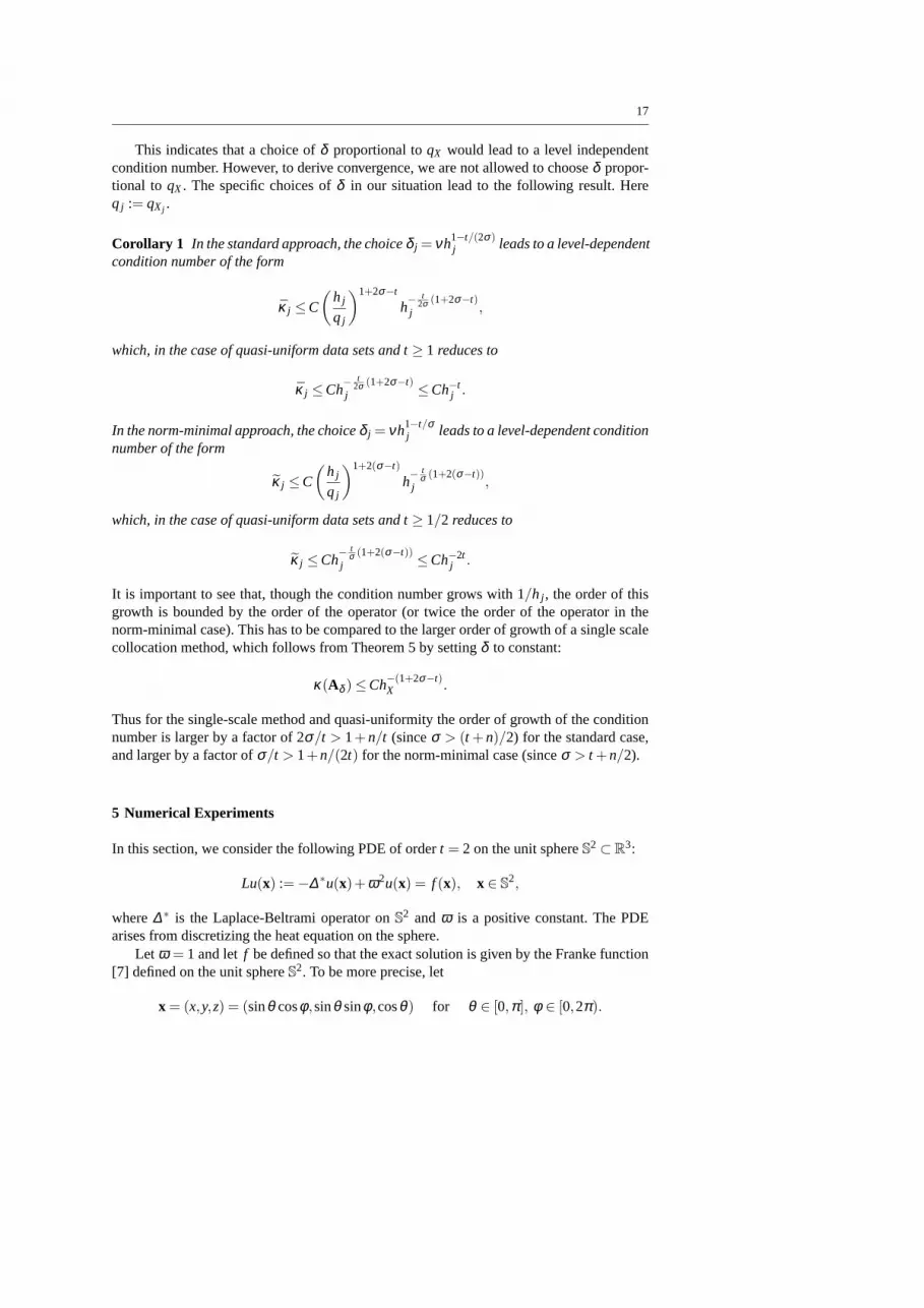
This indicates that a choice ofδ proportional toqX would lead to a level independentcondition number. However, to derive convergence, we are not allowed to chooseδ propor-tional to qX. The specific choices ofδ in our situation lead to the following result. Hereq j := qXj .

Corollary 1 In the standard approach, the choiceδ j = νh1−t/(2σ)j leads to a level-dependent

condition number of the form

κ j ≤C

(h j

q j

)1+2σ−t

h− t

2σ (1+2σ−t)j ,

which, in the case of quasi-uniform data sets and t≥ 1 reduces to

κ j ≤Ch− t

2σ (1+2σ−t)j ≤Ch−t

j .

In the norm-minimal approach, the choiceδ j = νh1−t/σj leads to a level-dependent condition

number of the form

κ j ≤C

(h j

q j

)1+2(σ−t)

h− t

σ (1+2(σ−t))j ,

which, in the case of quasi-uniform data sets and t≥ 1/2 reduces to

κ j ≤Ch− t

σ (1+2(σ−t))j ≤Ch−2t

j .

It is important to see that, though the condition number grows with 1/h j , the order of thisgrowth is bounded by the order of the operator (or twice the order of the operator in thenorm-minimal case). This has to be compared to the larger order of growth of a single scalecollocation method, which follows from Theorem 5 by settingδ to constant:

κ(Aδ ) ≤Ch−(1+2σ−t)X .

Thus for the single-scale method and quasi-uniformity the order of growth of the conditionnumber is larger by a factor of 2σ/t > 1+n/t (sinceσ > (t +n)/2) for the standard case,and larger by a factor ofσ/t > 1+n/(2t) for the norm-minimal case (sinceσ > t +n/2).

5 Numerical Experiments

In this section, we consider the following PDE of ordert = 2 on the unit sphereS2 ⊂ R3:

Lu(x) := −∆ ∗u(x)+ω2u(x) = f (x), x ∈ S2,

where∆ ∗ is the Laplace-Beltrami operator onS2 andω is a positive constant. The PDEarises from discretizing the heat equation on the sphere.

Let ω = 1 and letf be defined so that the exact solution is given by the Franke function[7] defined on the unit sphereS2. To be more precise, let

x = (x,y,z) = (sinθ cosφ ,sinθ sinφ ,cosθ) for θ ∈ [0,π], φ ∈ [0,2π).

18

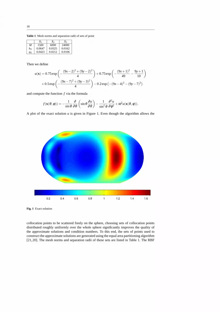
Table 1 Mesh norms and separation radii of sets of point

X1 X2 X3

M 1500 6000 24000hX 0.0647 0.0325 0.0162qX 0.0423 0.0212 0.0106

Then we define

u(x) = 0.75exp

(− (9x−2)2 +(9y−2)2

4

)+0.75exp

(− (9x+1)2

49− 9y+1

10

)

+0.5exp

(− (9x−7)2 +(9y−3)2

4

)−0.2exp

(−(9x−4)2− (9y−7)2)

and compute the functionf via the formula

f (x(θ ,φ)) = − 1sinθ

∂∂θ

(sinθ

∂u∂θ

)− 1

sin2 θ∂ 2u∂φ2 +ω2u(x(θ ,φ)).

A plot of the exact solutionu is given in Figure 1. Even though the algorithm allows the

Fig. 1 Exact solution

collocation points to be scattered freely on the sphere, choosing sets of collocation pointsdistributed roughly uniformly over the whole sphere significantly improves the quality ofthe approximate solutions and condition numbers. To this end, the sets of points used toconstruct the approximate solutions are generated using the equal area partitioning algorithm[21,20]. The mesh norms and separation radii of these sets are listed in Table 1. The RBF

19

used isψ(r) = (1− r)6

+(3+18r +35r2), ψδ (r) = δ−2ψ(r/δ ),

andΦδ (x,y) = ψδ (|x−y|) = ψδ (

√2−2x ·y).

It can be shown thatΦδ is a kernel which satisfies condition (7) withσ = 7/2 ([18]).The kernelΦδ is a zonal function, i.e.Φδ (x,y) = φδ (x · y) whereφδ (t) is a univariate

function. For zonal functions, the Laplace-Beltrami operator can be computed via

∆ ∗φδ (x ·y) = L φδ (t), t = x ·y,

where

L =ddt

(1− t2)ddt

In our case,

L φδ (t) =112δ 10 (

√2−2t −δ )4

(25t2−10t +δ 2t −15+

−8δ t2 +8δ t√2−2t

).

At each level the normalizedL2 error‖ej‖ is approximated by anℓ2 error, thus in principlewe define

‖ej‖ :=

(1

4π

∫

S2|u(x)−u j(x)|2dx

)1/2

=

(1

4π

∫ π

0

∫ 2π

0|u(θ ,φ)−u j(θ ,φ)|2sinθdφdθ

)1/2

,

and in practice approximate this by the midpoint rule at 1 degree intervals,(

14π

2π2

|G | ∑x(θ ,φ)∈G

|u(θ ,φ)−u j(θ ,φ)|2sinθ

)1/2

,

whereG is a longitude-latitude grid containing the centers of rectangles of size 1 degreetimes 1 degree and|G |= 180·360= 64800. We also record the condition numbersκ j of thecollocation matrix

Aδ j= [LΦ j(x,y)]x,y∈Xj

for the standard approach and the condition numbersκ j of the collocation matrix

Aδ j= [LLΦ j(x,y)]x,y∈Xj

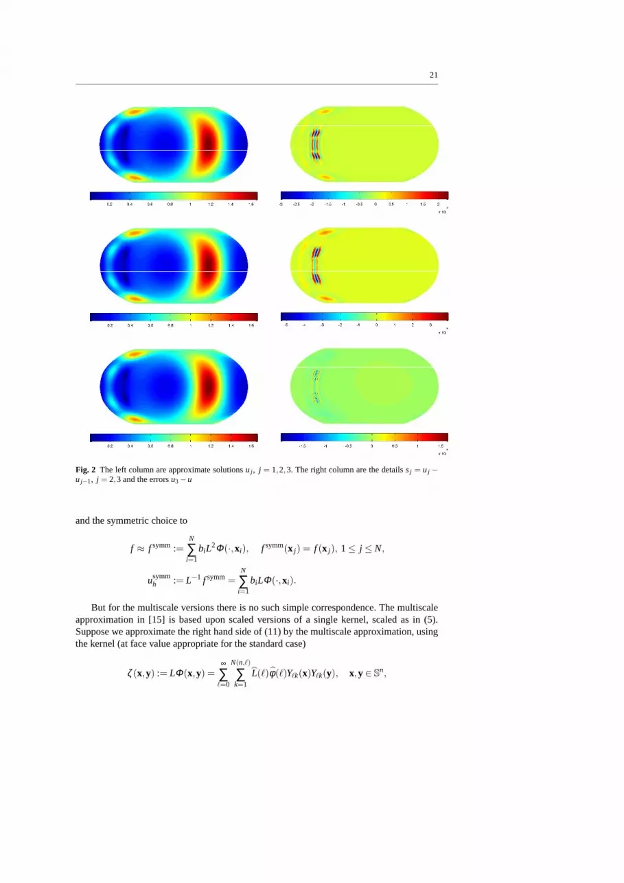
for the norm-minimal approach. The errors and condition numbers of the collocation matri-ces at each step of the multiscale algorithm for two variantsof the collocation method arelisted in Tables 2 and 3, respectively. In the upper part of each table we use the results for thescaleδ j taken proportional toh j , whereas in the lower part we use the scale in accordancewith Theorem 3 or 4. As can be seen from the tables, if the scaling parametersδ j decreaselinearly with respect to the mesh normsh j , we may not get a good convergence rate, atleast in the norm-minimal case, whereas in both cases we get agood convergence rate ifwe follow the theoretical predictions. Figure 2 shows the approximate solutions using thestandard approach at each level corresponding toδ j = 2;1.2230;0.7438, in accordance withTheorem 3. If we use one-shot approximation on the final set of24000 points with variousscalesδ then we obtain the errors listed in Tables 4 and 5. As can be seen from the tables,the multiscale approach provides a more accurate approximation with a collocation matrixof a smaller condition number.

20

Table 2 The approximation errors and condition numbers of multiscale approximation using the standardapproach

Level 1 2 3M 1500 6000 24000δ j 2.0 1.0 0.5‖ej‖ 2.1173E-04 3.9021E-06 1.1509E-07κ j 4.4028E+04 4.4172E+04 4.4562E+04δ j 2.0000 1.2230 0.7438‖ej‖ 2.1173E-04 3.8357E-06 1.0944E-07κ j 4.4028E+04 1.2154E+05 3.2279E+05

Table 3 The approximation errors and condition numbers of multiscale approximation using the norm-minimal approach

Level 1 2 3M 1500 6000 24000δ j 2.0 1.0 0.5‖ej‖ 5.1048E-02 3.4713E-02 3.3648E-02κ j 1.7471E+02 2.1987E+02 3.1605E+02δ j 2.0000 1.4820 1.1033‖ej‖ 5.1048E-02 7.2364E-03 2.6972E-04κ j 1.7471E+02 5.7738E+02 1.8929E+03

Table 4 Errors by one-shot approximation ofu with various scales using the final set of 24000 points (stan-dard approach)

δ 2.0000 1.2230 1.0000 0.7438 0.5000‖e‖ 1.1372E-07 2.8564E-07 1.0765E-06 8.4260E-06 1.3642E-04κ 4.6265E+07 3.9109E+06 1.4203E+06 3.2273E+05 4.4562E+04

Table 5 Errors by one-shot approximation ofu with various scales using the final set of 24000 points (norm-minimal approach)

δ 2.000 1.4820 1.1033 1.000 0.500‖e‖ 3.9640E-04 8.0738E-03 6.2875E-02 1.1298E-01 5.7892E-01κ 1.1200E+04 4.6228E+03 1.8927E+03 1.8927E+03 3.1605E+02

6 Concluding remarks

In this paper we have developed a multiscale approximation for elliptic PDEs on spheres,by adapting the method and the proof of the multiscale approximation scheme in [15].

A natural question is whether the scheme so developed is equivalent to applying themultiscale approximation scheme to the right hand side of equation (11), with an appropriateredefinition of the kernel.

For the single-scale collocation schemes withδ = 1 there is indeed a close connection,in that the standard and symmetric collocation schemes of Sections 3.1 and 3.2 can be re-expressed this way: the standard choice is equivalent to

f ≈ f stand:=N

∑i=1

biLΦ(·,xi), f stand(x j) = f (x j), 1≤ j ≤ N,

ustandh := L−1 f stand=

N

∑i=1

biΦ(·,xi),

21

Fig. 2 The left column are approximate solutionsu j , j = 1,2,3. The right column are the detailssj = u j −u j−1, j = 2,3 and the errorsu3−u

and the symmetric choice to

f ≈ f symm :=N

∑i=1

biL2Φ(·,xi), f symm(x j) = f (x j), 1≤ j ≤ N,

usymmh := L−1 f symm=

N

∑i=1

biLΦ(·,xi).

But for the multiscale versions there is no such simple correspondence. The multiscaleapproximation in [15] is based upon scaled versions of a single kernel, scaled as in (5).Suppose we approximate the right hand side of (11) by the multiscale approximation, usingthe kernel (at face value appropriate for the standard case)

ζ (x,y) := LΦ(x,y) =∞

∑ℓ=0

N(n,ℓ)

∑k=1

L(ℓ)φ(ℓ)Yℓk(x)Yℓk(y), x,y ∈ Sn,

22

We can define a scaled version of the new kernel after extending the definition toRn+1, butthe difficulty is that the scaled kernelζδ is not related in any simple way toLΦδ , even for thecaseL = −∆ +1. To state the problem differently, an effective multiscale method based onthe scaled kernelζδ would require an ability to solve analytically the equationLg= ζδ (·,xi),something that does not seem possible in general.

The multiscale method presented in Section 4 is therefore significantly different fromthe multiscale approximation in [15].

Acknowledgements The support of the Australian Research Council is gratefully acknowledged.

References

1. G. E. Fasshauer. Solving differential equations with radial basis functions: multilevel methods andsmoothing.Advances in Comput. Math., 11:139–159, 1999.

2. G. E. Fasshauer and J. W. Jerome. Multistep approximation algorithms: improved convergence ratesthrough postconditioning with smooth kernels.Advances in Comput. Math., 10:1–27, 1999.

3. N. Flyer and G. Wright. Transport schemes on a sphere using radial basis functions.J. Comp. Phys.,226:1059–1084, 2007.

4. N. Flyer and G. Wright. A radial basis function method for theshallow water equations on a sphere.Proc. R. Soc. A, 465:1949–1976, 2009.

5. C. Franke and R. Schaback. Convergence order estimates of meshless collocation methods using radialbasis functions.Adv. in Comp. Math., 8:381–399, 1998.

6. C. Franke and R. Schaback. Solving partial differential equations by collocation using radial basisfunctions.Appl. Math. Comput., 93:73–82, 1998.

7. R. Franke. A critical comparison of some methods for interpolation of scattered data. Technical ReportNPS-53-79-003, Naval Postgraduate School, 1979.

8. P. Giesl and H. Wendland. Meshless collocation: Error estimates with application to dynamical systems.SIAM J. Num. Analysis, 45:1723–1741, 2007.

9. Y. C. Hon and X. Z. Mao. An efficient numerical scheme for Burgers’ equation.Appl. Math. Comput.,95:37–50, 1998.

10. Y. C. Hon and R. Schaback. On unsymmetric collocation by radial basis functions.Appl. Math. Comput.,119:177–186, 2001.

11. E. J. Kansa. Multiquadrics - A scattered data approximation scheme with applications to computationalfluid-dynamics i.Comput. Math., 19:127–145, 1990.

12. E. J. Kansa. Multiquadrics - A scattered data approximation scheme with applications to computationalfluid-dynamics ii: solutions to parabolic, hyperbolic and elliptic partial differential equations.Comput.Math., 19:147–161, 1990.

13. Q. T. Le Gia. Galerkin approximation for elliptic PDEs on spheres.J. Approx. Theory, 130:123–147,2004.

14. Q. T. Le Gia, F. J. Narcowich, J. D. Ward, and H. Wendland. Continuous and discrete least-squareapproximation by radial basis functions on spheres.J. Approx. Theory, 143:124–133, 2006.

15. Q. T. Le Gia, I. H. Sloan, and H. Wendland. Multiscale analysis in Sobolev spaces on the sphere.SIAMJ. Numerical Analysis, 48:2065–2090, 2010.

16. T. M. Morton and M. Neamtu. Error bounds for solving pseudodifferential equations on spheres.J.Approx. Theory, 114:242–268, 2002.

17. C. Muller. Spherical Harmonics, volume 17 ofLecture Notes in Mathematics. Springer-Verlag, Berlin,1966.

18. F. J. Narcowich and J. D. Ward. Scattered data interpolation on spheres: error estimates and locallysupported basis functions.SIAM J. Math. Anal., 33:1393–1410, 2002.

19. H. Power and V. Barraco. A comparison analysis between unsymmetric and symmetric radial basisfunction collocation methods for the numerical solution of partial differential equations.Comput. Math.Appl., 43:551–583, 2002.

20. E. B. Saff and A. B. J. Kuijlaars. Distributing many pointson a sphere.Math. Intelligencer, 19:5–11,1997.

21. E. B. Saff, E. A. Rakhmanov, and Y. M. Zhou. Minimal discreteenergy on the sphere.MathematicalResearch Letters, 1:647–662, 1994.

22. I. J. Schoenberg. Positive definite function on spheres.Duke Math. J., 9:96–108, 1942.

23

23. H. Wendland. Meshless Galerkin methods using radial basis functions. Math. Comp., 68:1521–1531,1999.

24. H. Wendland.Scattered Data Approximation. Cambridge University Press, Cambridge, 2005.25. H. Wendland. Multiscale analysis in Sobolev spaces on bounded domains.Numerische Mathematik,

page (to appear), 2010.26. Y. Xu and E. W. Cheney. Strictly positive definite functions on spheres.Proc. Amer. Math. Soc., 116:977–

981, 1992.