Gypsilab : a MATLAB toolbox for FEM-BEMcoupling

François Alouges,(joint work with Matthieu Aussal)

Workshop on Numerical methods for wave propagation andapplications

Sept. 1st 2017

Facts

New numerical techniques in FEM (e.g. DDM) or BEM(compression techniques).Difficult to test them on different applications (equationsmight be quite complex).Numericians might not be specialists influid/elasticity/electromagnetic/acoustic/etc. domains.Difficult to transfer one technique that worked in a domainto another one.Difficult to transfer the new techniques to other people (e.g.companies).

FEM and BEM specificities

FEM leads to sparse matrices N unknowns O(N) storage(2D-3D)FEM softwares are numerous. Some are free (e.g.FreeFem++, GetDP, Xlife++, FENICS), others arecommercial products (COMSOL, Fluent, etc.).BEM leads to O(N2) storage (usually on the boundary 2D)BEM softwares are more rare (BEM++, Xlife++)BEM methods often need compression techniques (FMM,H-Matrices, SCSD) and singular integration techniques.This is often very technical.FEM-BEM coupling is even more difficult (coupling sparseand H-Matrices, direct vs iterative methods, etc.).

Prototyping languages

When one creates a new numerical technique it is practical tohave a prototyping environment (Matlab, Python, Julia).

FreeFem++ (Nice for FEM, no BEM yet)FENICS/FireDrake (FEM in Python, BEM++ is beinginterfaced)Julia ?Matlab : everybody has his own library for FEM, somepeople implement BEM

Need for a versatile easy to use toolbox “à la FreeFem++” forFEM-BEM

Gypsilab

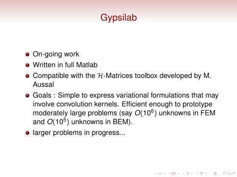
On-going workWritten in full MatlabCompatible with the H-Matrices toolbox developed by M.AussalGoals : Simple to express variational formulations that mayinvolve convolution kernels. Efficient enough to prototypemoderately large problems (say O(106) unknowns in FEMand O(105) unknowns in BEM).larger problems in progress...

Formalism

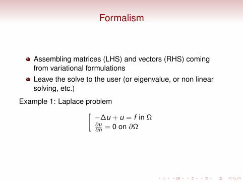
Assembling matrices (LHS) and vectors (RHS) comingfrom variational formulationsLeave the solve to the user (or eigenvalue, or non linearsolving, etc.)

Example 1: Laplace problem[−∆u + u = f in Ω∂u∂n = 0 on ∂Ω

Laplace example

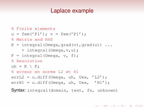
% Finite elementsu = fem(’P1’); v = fem(’P1’);% Matrix and RHSK = integral(Omega,grad(v),grad(u)) ...

+ integral(Omega,v,u);F = integral(Omega, v, f);% Resolutionuh = K \ F;% erreur en norme L2 et H1errL2 = u.diff(Omega, uh, Uex, ’L2’);errH1 = u.diff(Omega, uh, Uex, ’H1’);

Syntax: integral(domain, test, fn, unknown)

Full program

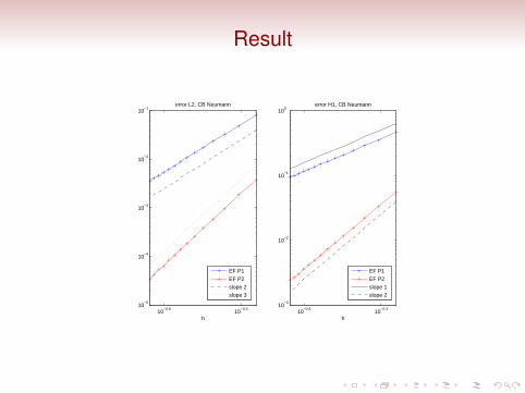
Result

10−0.8

10−0.3

10−5

10−4

10−3

10−2

10−1

h

error L2, CB Neumann

EF P1

EF P2

slope 2

slope 3

10−0.8

10−0.3

10−3

10−2

10−1

100

h

error H1, CB Neumann

EF P1

EF P2

slope 1

slope 2

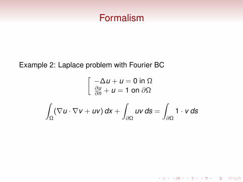
Formalism

Example 2: Laplace problem with Fourier BC[−∆u + u = 0 in Ω∂u∂n + u = 1 on ∂Ω∫

Ω(∇u · ∇v + uv) dx +

∫∂Ω

uv ds =

∫∂Ω

1 · v ds

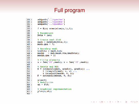
Full program

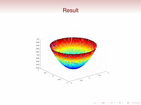
Result

−1

−0.5

0

0.5

1

−1

−0.5

0

0.5

10.52

0.54

0.56

0.58

0.6

0.62

0.64

0.66

0.68

0.7

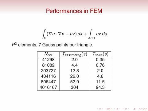
Performances in FEM

∫Ω

(∇u · ∇v + uv) dx +

∫∂Ω

uv ds

P2 elements, 7 Gauss points per triangle.

Ndof Tassembling(s) Tsolve(s)

41298 2.0 0.3581082 4.4 0.76

203727 12.3 2.0404116 26.0 4.6806447 52.9 11.5

4016167 304 94.3

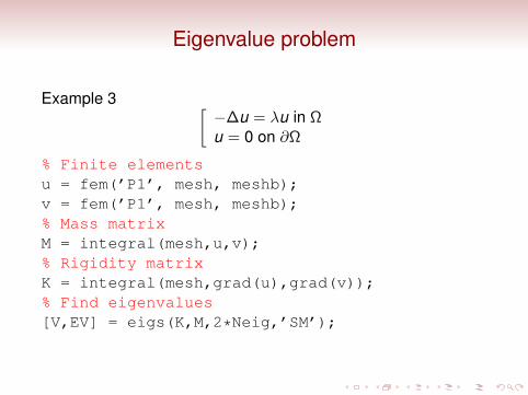
Eigenvalue problem

Example 3 [−∆u = λu in Ωu = 0 on ∂Ω

% Finite elementsu = fem(’P1’, mesh, meshb);v = fem(’P1’, mesh, meshb);% Mass matrixM = integral(mesh,u,v);% Rigidity matrixK = integral(mesh,grad(u),grad(v));% Find eigenvalues[V,EV] = eigs(K,M,2*Neig,’SM’);

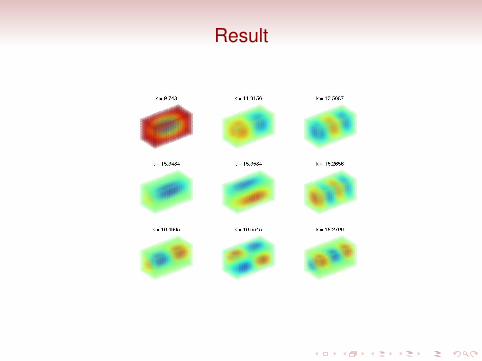
Result

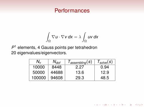
Performances

∫Ω∇u · ∇v dx = λ

∫Ω

uv dx

P1 elements, 4 Gauss points per tetrahedron20 eigenvalues/eigenvectors.

Nv Ndof Tassembling(s) Tsolve(s)

10000 8448 2.27 0.9450000 44688 13.6 12.9

100000 94608 29.3 48.5

Inside the box - FEM

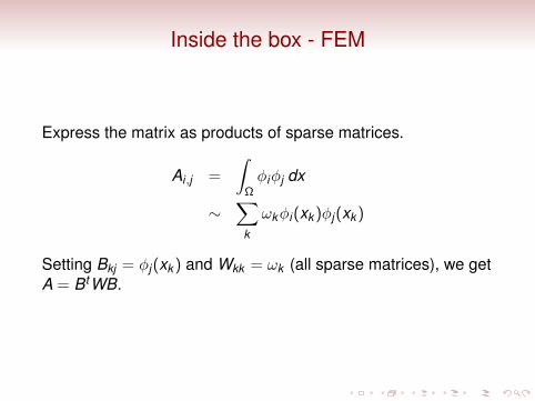
Express the matrix as products of sparse matrices.

Ai,j =

∫Ωφiφj dx

∼∑

k

ωkφi(xk )φj(xk )

Setting Bkj = φj(xk ) and Wkk = ωk (all sparse matrices), we getA = BtWB.

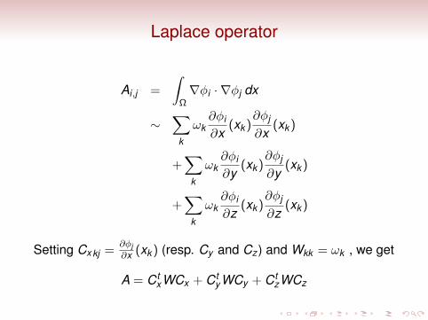
Laplace operator

Ai,j =

∫Ω∇φi · ∇φj dx

∼∑

k

ωk∂φi

∂x(xk )

∂φj

∂x(xk )

+∑

k

ωk∂φi

∂y(xk )

∂φj

∂y(xk )

+∑

k

ωk∂φi

∂z(xk )

∂φj

∂z(xk )

Setting Cx kj =∂φj∂x (xk ) (resp. Cy and Cz) and Wkk = ωk , we get

A = CtxWCx + Ct

yWCy + CtzWCz

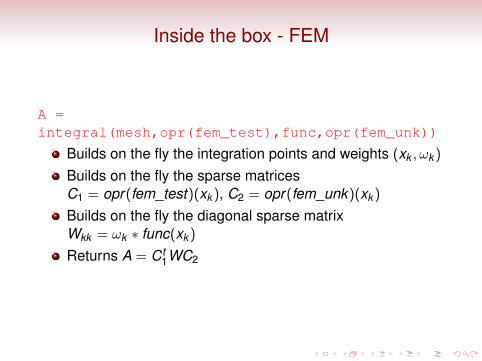
Inside the box - FEM

A =integral(mesh,opr(fem_test),func,opr(fem_unk))

Builds on the fly the integration points and weights (xk , ωk )

Builds on the fly the sparse matricesC1 = opr(fem_test)(xk ), C2 = opr(fem_unk)(xk )

Builds on the fly the diagonal sparse matrixWkk = ωk ∗ func(xk )

Returns A = Ct1WC2

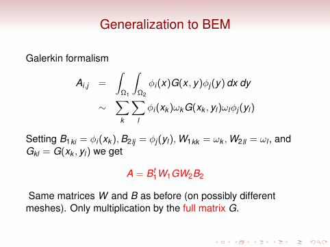
Generalization to BEM

Galerkin formalism

Ai,j =

∫Ω1

∫Ω2

φi(x)G(x , y)φj(y) dx dy

∼∑

k

∑l

φi(xk )ωkG(xk , yl)ωlφj(yl)

Setting B1ki = φi(xk ),B2lj = φj(yl),W1kk = ωk ,W2ll = ωl , andGkl = G(xk , yl) we get

A = Bt1W1GW2B2

Same matrices W and B as before (on possibly differentmeshes). Only multiplication by the full matrix G.

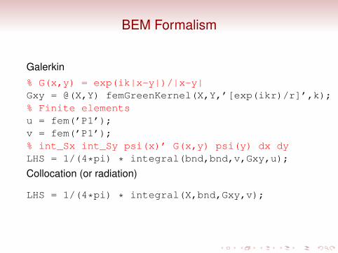
BEM Formalism

Galerkin% G(x,y) = exp(ik|x-y|)/|x-y|Gxy = @(X,Y) femGreenKernel(X,Y,’[exp(ikr)/r]’,k);% Finite elementsu = fem(’P1’);v = fem(’P1’);% int_Sx int_Sy psi(x)’ G(x,y) psi(y) dx dyLHS = 1/(4*pi) * integral(bnd,bnd,v,Gxy,u);

Collocation (or radiation)

LHS = 1/(4*pi) * integral(X,bnd,Gxy,v);

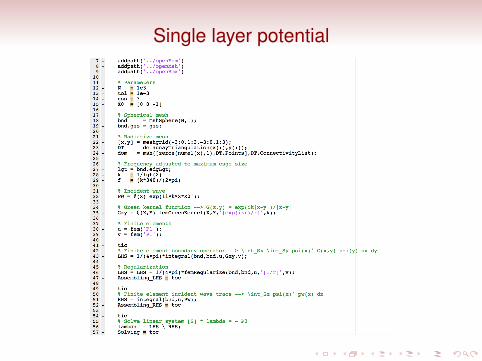
Single layer potential

Single layer potential

0 1 2 3 4 5 6 7−1

−0.5

0

0.5

1

1.5

−0.50

0.5

−3

−2

−1

0

1

2

3−3

−2

−1

0

1

2

3

Total field solution

0.2

0.4

0.6

0.8

1

1.2

1.4

1.6

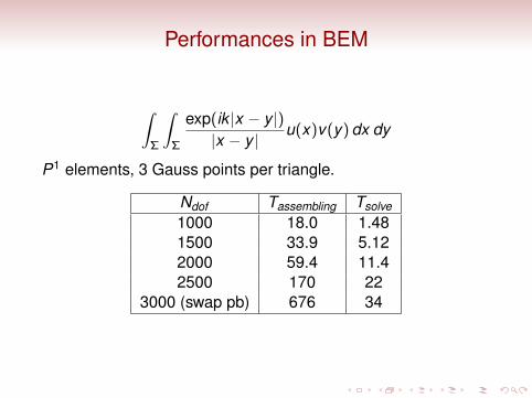
Performances in BEM

∫Σ

∫Σ

exp(ik |x − y |)|x − y |

u(x)v(y) dx dy

P1 elements, 3 Gauss points per triangle.

Ndof Tassembling Tsolve1000 18.0 1.481500 33.9 5.122000 59.4 11.42500 170 22

3000 (swap pb) 676 34

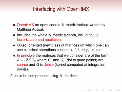
Interfacing with OpenHMX

OpenHMX an open source H-matrix toolbox written byMatthieu Aussal.Includes the whole H-matrix algebra, including LUfactorization and resolution.Object oriented (new class of matrices on which one canuse classical operations such as +, *, \, spy, lu, etc.In principle the matrices that we consider are of the formA = Ct

1GC2 where C1 and C2 (dof to quad points) aresparse and G is dense (kernel computed at integrationpoints).

G could be compressed using H-matrices...

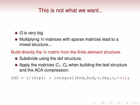
This is not what we want..

G is very big.Multiplying H-matrices with sparse matrices lead to amixed structure...

Build directly the H-matrix from the finite element structure.Subdivide using the dof structure.Apply the matrices C1, C2 when building the leaf structureand the ACA compression.

LHS = 1/(4*pi) * integral(bnd,bnd,v,Gxy,u,tol);

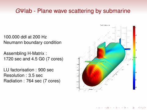
GΨlab - Plane wave scattering by submarine

100.000 ddl at 200 HzNeumann boundary condition

Assembling H-Matrix :1720 sec and 4.5 G0 (7 cores)

LU factorisation : 900 secResolution : 3.5 secRadiation : 764 sec (7 cores)

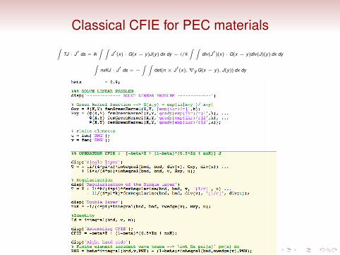
Classical CFIE for PEC materials∫

TJ · J′ ds = ik∫ ∫

J′(x) · G(x − y)J(y) dx dy − i/k∫ ∫

div(J′)(x) · G(x − y)div(J)(y) dx dy

∫nxKJ · J′ ds = −

∫ ∫det(n × J′(x),∇y G(x − y), J(y)) dx dy

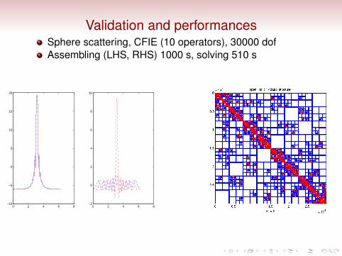
Validation and performancesSphere scattering, CFIE (10 operators), 30000 dofAssembling (LHS, RHS) 1000 s, solving 510 s

0 2 4 6 8−10

−5

0

5

10

15

20

0 2 4 6 8−2

0

2

4

6

8

10

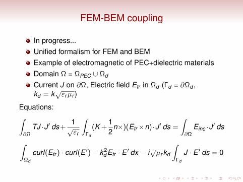
FEM-BEM coupling

In progress...Unified formalism for FEM and BEMExample of electromagnetic of PEC+dielectric materialsDomain Ω = ΩPEC ∪ Ωd

Current J on ∂Ω, Electric field Etr in Ωd (Γd = ∂Ωd ,kd = k

√εrµr )

Equations:∫∂Ω

TJ ·J ′ ds+1√εr

∫Γd

(K +12

n×)(Etr×n) ·J ′ ds =

∫∂Ω

Einc ·J ′ ds

∫Ωd

curl(Etr ) · curl(E ′)− k2d Etr · E ′ dx − i

õr kd

∫Γd

J · E ′ ds = 0

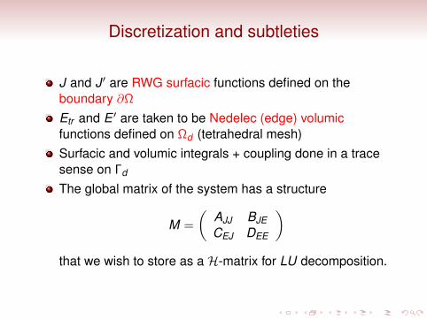
Discretization and subtleties

J and J ′ are RWG surfacic functions defined on theboundary ∂Ω

Etr and E ′ are taken to be Nedelec (edge) volumicfunctions defined on Ωd (tetrahedral mesh)Surfacic and volumic integrals + coupling done in a tracesense on Γd

The global matrix of the system has a structure

M =

(AJJ BJECEJ DEE

)that we wish to store as a H-matrix for LU decomposition.

Conclusion

GΨlab is a matlab toolbox for FEM-BEM programmingEasy to use interfaceIncludes H-matrix toolboxGΨlab is open source (GPL like license), downloadable atwww.cmap.polytechnique.fr/˜aussal/gypsilab