an evolutionary programming algorithm for solving unit

Journal of Renewable Energy and Smart Grid Technology, Vol. 16, No. 1, January-June 2021

An Evolutionary Programming Algorithm for Solving Unit Commitment

Problem in Smart Grid Environment

Charles Christober Asir Rajan

Department of EEE, Puducherry Technological University, Puducherry 605014, India

Corresponding author’s email: [email protected]

Received: 12/12/2020, Accepted: 11/06/2021

Abstract

This paper presents a new approach to solving the unit commitment problem using Evolutionary

Programming Algorithm (EPA) in smart grid environment. The objective of this paper is to find the

generation scheduling such that the total operating cost can be minimized, when subjected to a variety

of constraints. This also means that it is desirable to find the optimal generating unit commitment in the

power system for the next H hours. This paper proposes distributed sources which includes electric

vehicles and distributed generation. EPA, which happens to be a Global Optimisation technique for

solving Unit Commitment Problem, operates on a system, which is designed to encode each unit’s

operating schedule with regard to its minimum up/down time. In this, the unit commitment schedule is

coded as a string of symbols. An initial population of parent solutions is generated at random. Here,

each schedule is formed by committing all the units according to their initial status (“flat start”). Here

the parents are obtained from a pre-defined set of solution’s i.e. each and every solution is adjusted to

meet the requirements. Then, a random recommitment is carried out with respect to the unit’s minimum

down times. The Neyveli Thermal Power Station (NTPS) Unit - II in India demonstrates the

effectiveness of the proposed approach; extensive studies have also been performed for different power

systems consists of IEEE 10, 26, 34 generating units. Numerical results are shown comparing the cost

solutions and computation time obtained by using the EPA and other conventional methods like

Dynamic Programming, Legrangian Relaxation and Simulated Annealing and Tabu Search in reaching

proper unit commitment.

Keywords: Unit Commitment, Evolutionary Programming, Simulated Annealing, Legrangian Relaxation,

Dynamic Programming

1. Introduction

Power Stations and electricity generating companies and power systems has the problem of deciding

how best to meet the varying demand for electricity, which has a daily and weekly cycle. The short-term

optimisation problem is how to schedule generation to minimize the total fuel cost or to maximize the

total profit over a study period of typically a day, subject to a large number of constraints that must be

satisfied. The daily load pattern for a given system may exhibit large differences between minimum and

maximum demand. Therefore, enough reliable power generation to meet the peak load demand must

therefore be synchronized prior to the actual occurrence of the load. Thus it is clear that it is not proper

and economical to run all the units available all the time. Since the load varies continuously with time,

the optimum condition of units may alter during any period. Therefore, the problem of determining the

units of a plant that should operate for a given load is the problem of unit commitment. For total number

of units of higher order, the problems associated with unit commitment have generally been difficult to

solve because of uncertainty of particular aspects of the problem. For instance, the availability of fuel in

precise, load forecast variable costs affected by the loading of generator units and the losses caused by

reactive flows are some of the unpredictable issues. There are other problems of inconsistency that affect

mailto:[email protected]


52

the overall economic operation of the electric power station. In order to reach a feasible solution for Unit

Commitment Problem (UCP), different considerations must be considered.

Research endeavours, therefore, have been focused on; efficient, near-optimal UC algorithms, which

can be applied to large-scale, power systems and have reasonable storage and computation time

requirements. A survey of existing literature [1-33] on the problem reveals that various numerical

optimisation techniques have been employed to approach the complicated unit commitment problem.

More specifically, these are the Dynamic Programming method (DP), the Mixed Integer Programming

method (MIP), the Lagrangian relaxation method (LR), the Branch and Bound method (BB), the Expert

system (ES), the Fuzzy Theorem method (FT), the Hop Field method (H), the Simulated Annealing

method (SA), the Tabu Search (TS), the Genetic Algorithm (GA), the Artificial Neural Network (ANN),

the Cuckoo Optimization Algorithm (COA) and so on. The major limitations of the numerical techniques

are the problem dimensions, large computational time and complexity in programming.

The DP method [1-2,13] is flexible but the disadvantage is the “curse of dimensionality”, which

results it may leads to more mathematical complexity and increase in computation time if the constraints

are taken in to consideration. The MIP methods [3-4] for solving the unit commitment problems fail

when the number of units increases because they require a large memory and suffer from great

computational delay. The LR approach [5-8] to solve the short-term UC Problems was found that it

provides faster solution but it will fail to obtain solution feasibility and solution quality problems and

becomes complex if the number of units increased. The BB method [9] employs a linear function to

represent fuel cost and start-up cost and obtains a lower and upper bounds. The difficulty of this method

is the exponential growth in the execution time for systems of a practical size. An ES algorithm [10,13]

rectifies the complexity in calculations and saving in computation time. But it will face the problem if

the new schedule is differing from schedule in database. In the FT method [11, 13, 24] using fuzzy set

solves the forecasted load schedules error but it will also suffer from complexity. The H neural network

technique [12] considers more constraints but it may suffer from numerical convergence due to its

training process. SA [14-17,23-24] is a powerful, general-purpose stochastic optimisation technique,

which can theoretically converge asymptotically to a global optimum solution with probability one. But

it will take much time to reach the near-global minimum. The TS [18-20, 23] is an iterative improvement

procedure that starts from some initial feasible solution and attempts to determine a better solution in the

manner of a greatest – decent algorithm. However, TS is characterized by an ability to escape local optima

by using a short-term memory of recent solutions.

GA [13,21-24] is a general-purpose stochastic and parallel search method based on the mechanics

of natural selection and natural genetics. It is a search method to have potential of obtaining near-global

minimum. And it has the capability to obtain the accurate results within short time and the constraints

are included easily. The ANN [12] has the advantages of giving good solution quality and rapid

convergence. And this method can accommodate more complicated unit-wise constraints and are claimed

for numerical convergence and solution quality problems. The solution processing in each method is very

unique. The EP [25-26] has the advantages of good convergent property and a significant speedup over

traditional GA’s and can obtain high quality solutions. The “Curse of dimensionality” is surmounted, and

the computational burden is almost linear with the problem scale. Electric Vehicle (EV) and its impact

on the cost and emission of power system are studied on basis of UC model in [28–30]. The significance

and feasibility of DR and its role in supply-demand schedule are examined in [31–32]. Economical

operation of distributed generation (DG) and chance-constrained schedule of active network with DG are

researched [33].

From the literature review, it has been observed that there exists a need for evolving simple and

effective methods, for obtaining an optimal solution for the UCP. Hence, in this paper, an attempt has

been made to EPA for meeting these requirements of the UCP, which eliminates the above-mentioned

drawbacks. EPA seems to be promising and is still evolving. EPA has the great advantage of good

convergent property and, hence, the computation time is considerably reduced. EPA is capable of

determining the global or near global solution. It is based on the basic genetic operation of human


53

chromosomes. It operates with the stochastic mechanics, which combine offspring creation based on

the performance of current trail solutions and competition and selection based on the successive

generations, form a considerably robust scheme for large-scale real-valued combinational optimisation.

In this proposed work, the parents are obtained from a pre-defined set of solution’s i.e. each and every

solution is adjusted to meet the requirements. And the selection process is done using Evolutionary

Strategy [25-26]. The application on the NTPS and IEEE systems consists of 10, 26, 34 generating

units’ shows that we can find the optimal solution effectively and these results are compared with the

conventional methods.

2. Problem Formulation

2.1. Smart Grid Environment

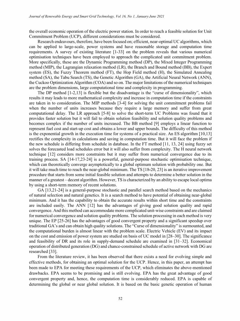
With the progress of smart grid, DR become more active. They may play an increasingly essential

part in power system operation. In this paper, EV and DG are considered in the UC model.

1) EV: Smart grid is a perfect platform for the collaborations between the system operators and

EVs. With the associated techniques getting settled, it is feasible for EV to sold electricity back to the

grid. There is fictional to be an aggregator to link between the system operator and a great number of

EV owners [28-30]. If an EV is indolent for a certain period, its owner can sign a contract with the

system operator for commitment via the load aggregator. The sum of EV can be preserved as a special

unit. Considering there is an increasing peripheral cost to involve more EV proprietors, the cost function

of EV is expected to be a quadratic function

EVeTC(EVek) = a1 + b1EVek + c1EVek2

(1)

where:

EVeTC = EV export total cost

EVek = EV export at time k

a1, b1EVek, c1EVek = cost coefficients of EV export at time k

Firstly, in case of emergent use of EV’s owners, a lower limit of SoC is considered (2). Secondly,

for the sake of safe operation of the gird, an upper limit on total output of EVs at each hour should be

stipulated (4). Thirdly, now that EV may not be connected to the grid all the 24 h, it is sensible to set a

time range limit when EV is available for the system operator (5). Fourthly, the available capacity of

EVe at each hour has an upper limit, respectively.

SoCk,t≥SoCmin (2)

k

k

x

tx

k

x

txko

tkC

EVeEViC

SoC==

−+

= 1

,

1

,,

,

(3)

EVek=∑EVek,t≤

m

t=1

EVemax

(4)


54

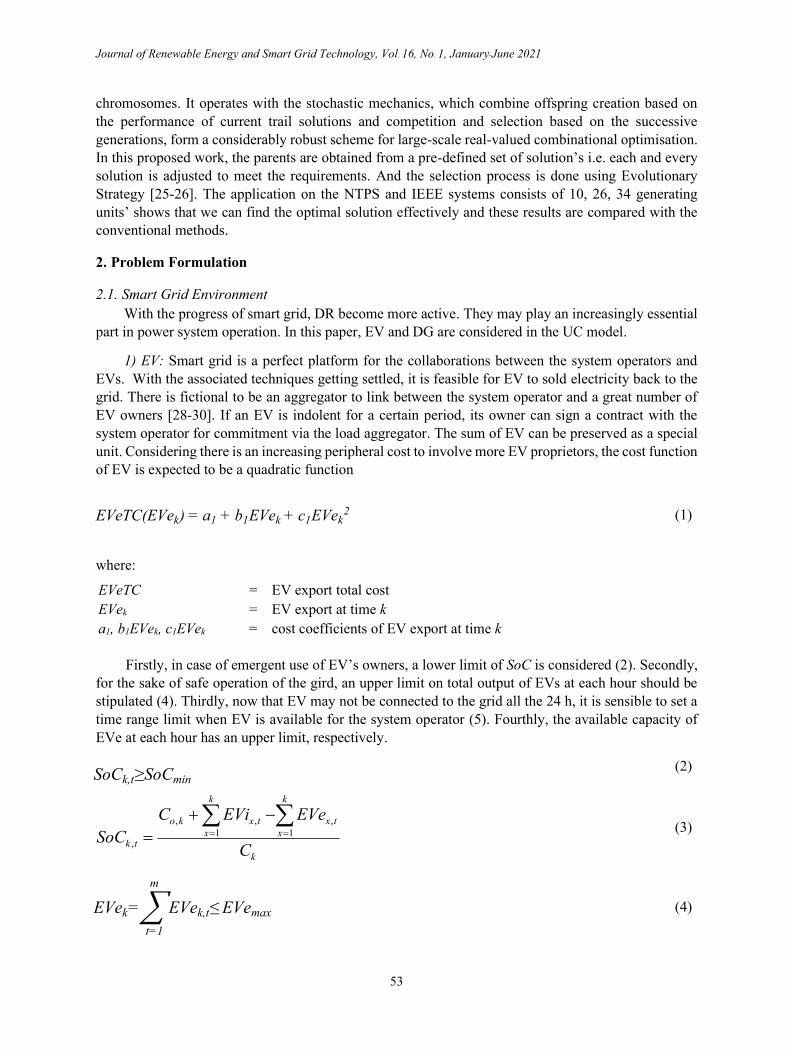
],[,0 21, kkkEVe tk =

(5)

EVek≤EVek,max (6)

where:

SoC = state of charge of EV

SoCk,t = state of charge of EV t at time k

SoCmin = minimum limit of SoC at each hour

Co,k = initial charging state of EV at time k

EVek,t = EV export t at time k

EVemax = maximum limit of EV export capacity

EVek,max = maximum available EV export capacity at time k

2) DG: When more DG’s are connected to the grid, then both importing and exporting power from

and to the DG’s should be taken into consideration in the UC model. Here the power can be sold to grid

is DGe and the power purchased from the grid is DGi. The cost function of the DG is expected to be a

quadratic equation

2

111)( kkk DGecDGebaDGeDG ++= (7)

where:

DGek = DG export at time k

a1, b1DGek, c1DGek = cost coefficients of DG

Firstly, DG’s output is subject to natural resource and weather condition, so an upper limit on

available DG at each hour is considered. Secondly, DG tends to be intermittent and volatile, an upper

limit on its penetration rate should be set to ensure a reliable operation of the power system

DGek≤DGek,max

(8)

ηk=

DGek

∑ (Pi,kIi,k)+EVek+DGekNi=1

≤ηmax

(9)

where:

2.2. UC Model

The objective is to find the generation scheduling such that the total operating cost can be

minimized, when subjected to a variety of constraints [27]. In the UCP under consideration, an

interesting solution would be minimizing the total operating cost of the generating units with several

constraints being satisfied. The major component of the operating cost, for thermal and nuclear units, is

the power production cost of the committed units and this is given in a quadratic form in (10).

DGek,max = maximum available DG export capacity at time k

ηk = penetration rate of DG at time t

ηmax = max penetration rate of DG at time t

Pi,k = output of unit i at time k

Ii,k = on/off status of unit I at time k


55

hrRsCPBPAPF iitiitiitit /)( 2 ++= (10)

where:

The startup cost depends upon the down time of the unit, which can vary from a maximum value,

when the unit i is started from cold state, to a much smaller value, if the unit i has been turned off

recently. The startup cost calculation depends upon the treatment method for the thermal unit during

down time periods. The start-up cost Sit, is a function of the down time of unit i as given in (11).

where:

The overall objective function of the UCP is given in (12).

== =

+++=24

11 1

/)]()([)])([(k

kk

T

t

N

i

itititititT HrRsDGeDGEVeEVeVSUPFF (12)

where:

2.3. Constraints

Depending on the nature of the power system under study, the UCP is subject to many constraints,

the main being the load balance constraints and the spinning reserve constraints. The other constraints

include the thermal constraints, fuel constraints, security constraints etc. [27]

1) Load Balance Constraints

The real power generated must be sufficient enough to meet the load demand and must satisfy

the following factors given in (13).

=

+−−−=N

i

kkkktitit PLDGeDGiEVePDUP1

(13)

where:

Ai, Bi, Ci = the cost function parameters of unit i (Rs./MW2hr, Rs./MWhr, Rs/hr)

Fit(Pit ) = production cost of unit i at a time t (Rs/hr)

Pit = output power from unit i at time t (MW)

Sit = Soi[1-Di exp ( -Toffi / Tdowni)] + Ei Rs (11)

Soi = unit i cold start – up cost (Rs)

Di, Ei = start – up cost coefficients for unit i

Uit = unit i status at hour t =1(if unit is ON) =0 (if unit is OFF)

Vit = unit i start up / shut down status at hour t =1 if the unit is started at hour t and 0 otherwise

FT = total operating cost over the schedule horizon (Rs/Hr)

Sit = start up cost of unit i at hour t (Rs)

PDt = system peak demand at hour t (MW)

N = number of available generating units

U (0,1) = the uniform distribution with parameters 0 and 1

UD (a,b) = the discrete uniform distribution with parameters a and b


56

2) Spinning Reserve Constraints

The spinning reserve is the total amount of real power generation available from all

synchronized units minus the present load plus the losses. The reserve is considered to be a pre

specified amount or a given percentage of the forecasted peak demand. It must be sufficient enough to

meet the loss of the most heavily loaded unit in the system. This has to satisfy the equation given in

(14).

=

+N

i

ttiti TtRPDUP1

1);(max (14)

where:

3) Thermal Constraints

The temperature and pressure of the thermal units vary very gradually and the units must be

synchronized before they are brought online. A time period of even 1 hour is considered as the minimum

down time of the units. There are certain factors, which govern the thermal constraints, like minimum

up time, minimum down time and crew constraints.

a) Minimum up time:

If the units have already been shut down, there will be a minimum time before they can be

restarted and the constraint is given in (15).

Toni ≥ Tupi (15)

where:

b) Minimum down time:

If all the units are running already, they cannot be shut down simultaneously and the

constraint is given in (16).

where:

4) Must Run Units

Generally in a power system, some of the units are given a must run status in order to provide

voltage support for the network.

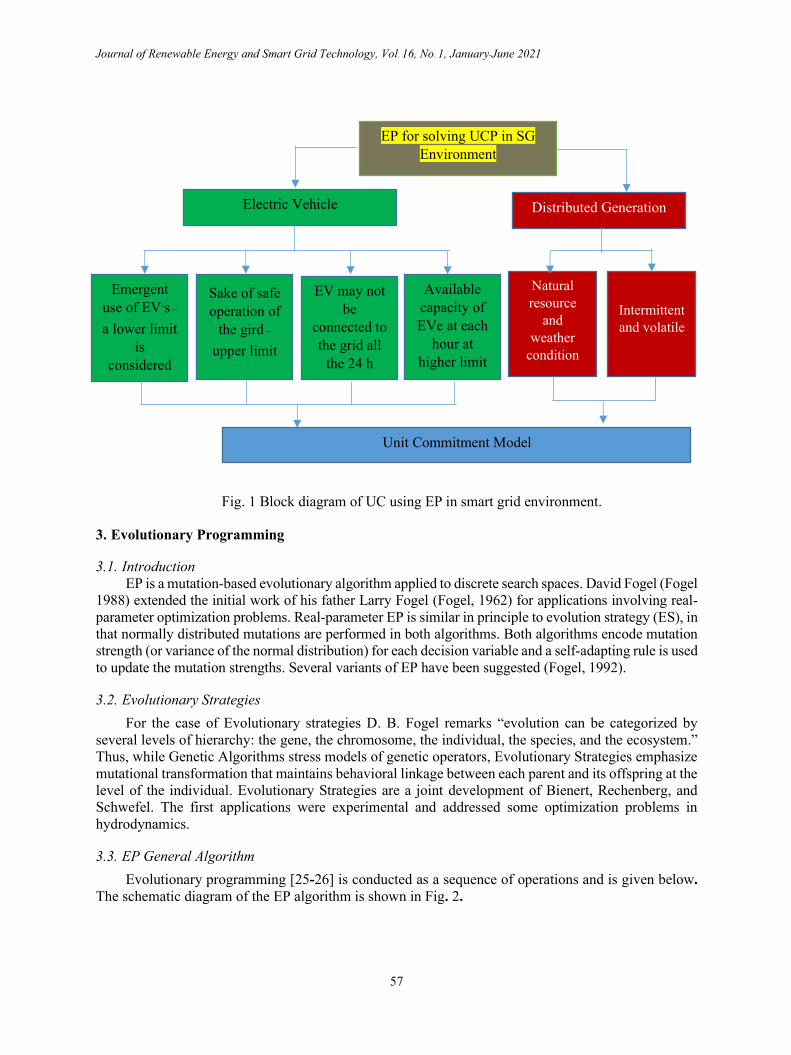
The entire problem formulation for solving the UC using EP in Smart Grid environment is

formulated as block diagram and is shown in Fig. 1.

Pmaxi = Maximum generation limit of unit i

Rt = spinning reserve at time t (MW)

T = scheduled time horizon (24 hr)

Toni = duration for which unit i is continuously ON (Hr)

Tupi = unit i minimum up time (Hr)

Toffi ≥ Tdowni (16)

Tdowni = unit i minimum down time (Hr)

Toffi = duration for which unit i is continuously OFF (Hr)


57

Fig. 1 Block diagram of UC using EP in smart grid environment.

3. Evolutionary Programming

3.1. Introduction

EP is a mutation-based evolutionary algorithm applied to discrete search spaces. David Fogel (Fogel

1988) extended the initial work of his father Larry Fogel (Fogel, 1962) for applications involving real-

parameter optimization problems. Real-parameter EP is similar in principle to evolution strategy (ES), in

that normally distributed mutations are performed in both algorithms. Both algorithms encode mutation

strength (or variance of the normal distribution) for each decision variable and a self-adapting rule is used

to update the mutation strengths. Several variants of EP have been suggested (Fogel, 1992).

3.2. Evolutionary Strategies

For the case of Evolutionary strategies D. B. Fogel remarks “evolution can be categorized by

several levels of hierarchy: the gene, the chromosome, the individual, the species, and the ecosystem.”

Thus, while Genetic Algorithms stress models of genetic operators, Evolutionary Strategies emphasize

mutational transformation that maintains behavioral linkage between each parent and its offspring at the

level of the individual. Evolutionary Strategies are a joint development of Bienert, Rechenberg, and

Schwefel. The first applications were experimental and addressed some optimization problems in

hydrodynamics.

3.3. EP General Algorithm

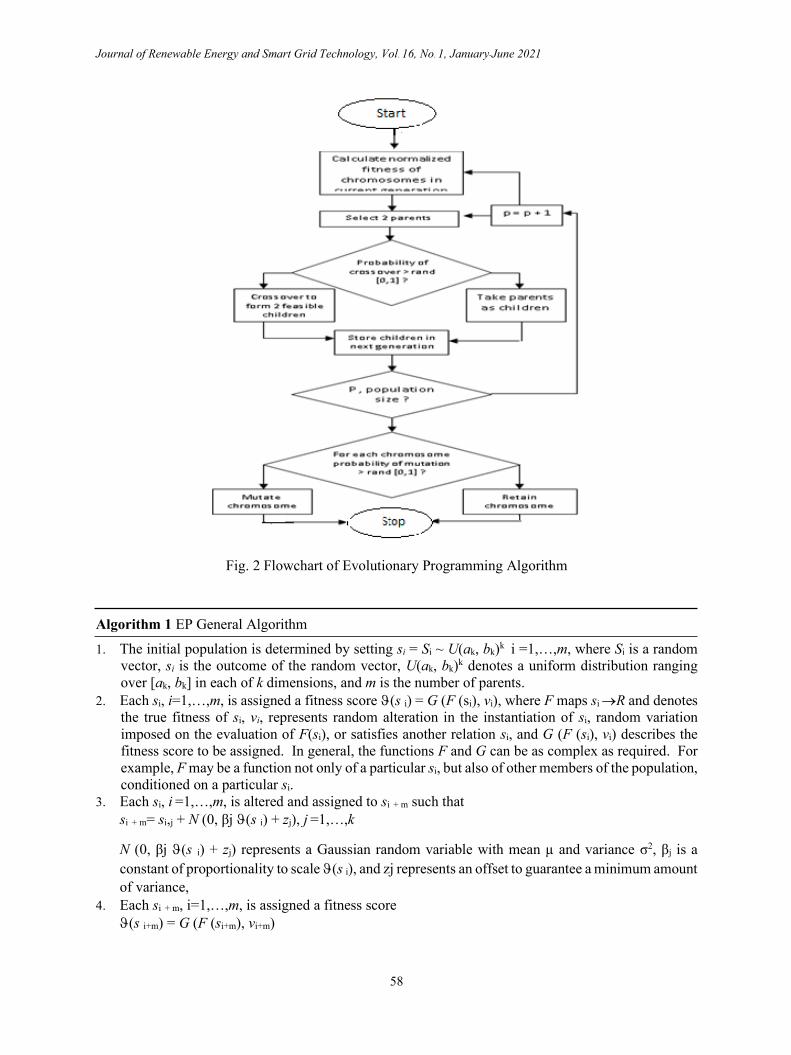
Evolutionary programming [25-26] is conducted as a sequence of operations and is given below.

The schematic diagram of the EP algorithm is shown in Fig. 2.

EP for solving UCP in SG

Environment

Electric Vehicle Distributed Generation

Emergent

use of EV’s –

a lower limit

is

considered

Available

capacity of

EVe at each

hour at

higher limit

EV may not

be

connected to

the grid all

the 24 h

Sake of safe

operation of

the gird – upper limit

Natural

resource

and

weather

condition

Intermittent

and volatile

Unit Commitment Model


58

Fig. 2 Flowchart of Evolutionary Programming Algorithm

Algorithm 1 EP General Algorithm

1. The initial population is determined by setting si = Si ~ U(ak, bk)k i =1,…,m, where Si is a random

vector, si is the outcome of the random vector, U(ak, bk)k denotes a uniform distribution ranging

over [ak, bk] in each of k dimensions, and m is the number of parents.

2. Each si, i=1,…,m, is assigned a fitness score (s i) = G (F (si), vi), where F maps si →R and denotes

the true fitness of si, vi, represents random alteration in the instantiation of si, random variation

imposed on the evaluation of F(si), or satisfies another relation si, and G (F (si), vi) describes the

fitness score to be assigned. In general, the functions F and G can be as complex as required. For

example, F may be a function not only of a particular si, but also of other members of the population,

conditioned on a particular si.

3. Each si, i =1,…,m, is altered and assigned to si + m such that

si + m= si,j + N (0, βj (s i) + zj), j =1,…,k

N (0, βj (s i) + zj) represents a Gaussian random variable with mean µ and variance σ2, βj is a

constant of proportionality to scale (s i), and zj represents an offset to guarantee a minimum amount

of variance,

4. Each si + m, i=1,…,m, is assigned a fitness score

(s i+m) = G (F (si+m), vi+m)


59

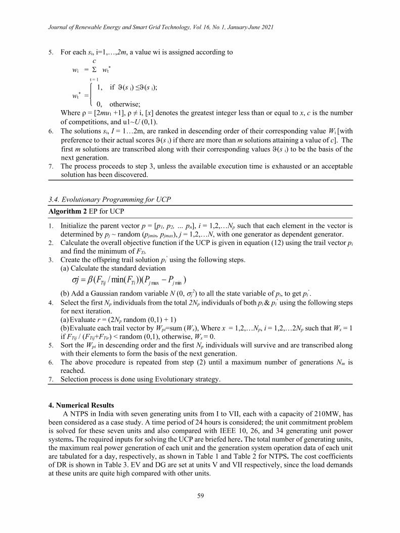
5. For each si, i=1,…,2m, a value wi is assigned according to

c

wi = wt*

t = 1

1, if (s i) ≤(s i);

wt* =

0, otherwise;

Where ρ = [2mu1 +1], ρ ≠ i, [x] denotes the greatest integer less than or equal to x, c is the number

of competitions, and u1~U (0,1).

6. The solutions si, I = 1…2m, are ranked in descending order of their corresponding value Wi [with

preference to their actual scores (s i) if there are more than m solutions attaining a value of c]. The

first m solutions are transcribed along with their corresponding values (s i) to be the basis of the

next generation.

7. The process proceeds to step 3, unless the available execution time is exhausted or an acceptable

solution has been discovered.

3.4. Evolutionary Programming for UCP

Algorithm 2 EP for UCP

1. Initialize the parent vector p = [p1, p2, … pn], i = 1,2,…Np such that each element in the vector is

determined by pj ~ random (pjmin, pjmax), j = 1,2,…N, with one generator as dependent generator.

2. Calculate the overall objective function if the UCP is given in equation (12) using the trail vector pi

and find the minimum of FTi.

3. Create the offspring trail solution pi’ using the following steps.

(a) Calculate the standard deviation

)))(min(/( minmax jjTiTij PPFFj −=

(b) Add a Gaussian random variable N (0, j2) to all the state variable of pi, to get pi

’.

4. Select the first Np individuals from the total 2Np individuals of both pi & pi’ using the following steps

for next iteration.

(a) Evaluate r = (2Np random (0,1) + 1)

(b) Evaluate each trail vector by Wpi=sum (Wx), Where x = 1,2,…Np, i = 1,2,…2Np such that Wx = 1

if FTij / (FTij+FTir) < random (0,1), otherwise, Wx = 0.

5. Sort the Wpi in descending order and the first Np individuals will survive and are transcribed along

with their elements to form the basis of the next generation.

6. The above procedure is repeated from step (2) until a maximum number of generations Nm is

reached.

7. Selection process is done using Evolutionary strategy.

4. Numerical Results

A NTPS in India with seven generating units from I to VII, each with a capacity of 210MW, has

been considered as a case study. A time period of 24 hours is considered; the unit commitment problem

is solved for these seven units and also compared with IEEE 10, 26, and 34 generating unit power

systems. The required inputs for solving the UCP are briefed here. The total number of generating units,

the maximum real power generation of each unit and the generation system operation data of each unit

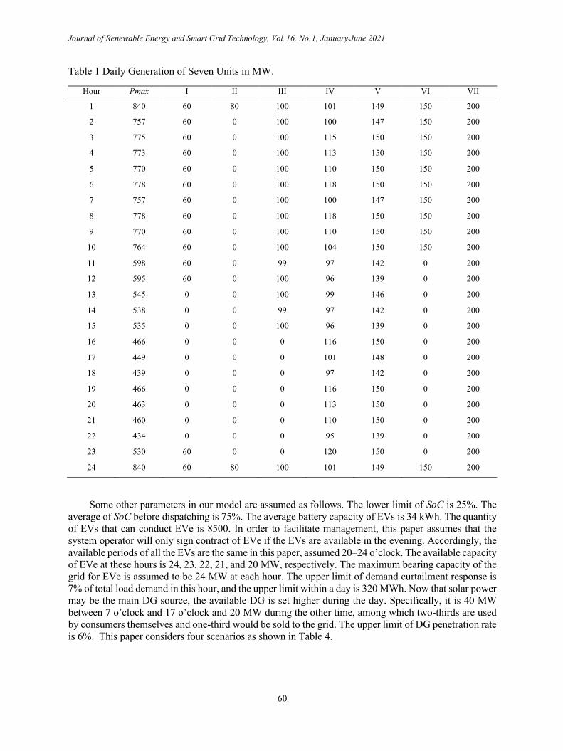
are tabulated for a day, respectively, as shown in Table 1 and Table 2 for NTPS. The cost coefficients

of DR is shown in Table 3. EV and DG are set at units V and VII respectively, since the load demands

at these units are quite high compared with other units.


60

Table 1 Daily Generation of Seven Units in MW.

Hour Pmax I II III IV V VI VII

1 840 60 80 100 101 149 150 200

2 757 60 0 100 100 147 150 200

3 775 60 0 100 115 150 150 200

4 773 60 0 100 113 150 150 200

5 770 60 0 100 110 150 150 200

6 778 60 0 100 118 150 150 200

7 757 60 0 100 100 147 150 200

8 778 60 0 100 118 150 150 200

9 770 60 0 100 110 150 150 200

10 764 60 0 100 104 150 150 200

11 598 60 0 99 97 142 0 200

12 595 60 0 100 96 139 0 200

13 545 0 0 100 99 146 0 200

14 538 0 0 99 97 142 0 200

15 535 0 0 100 96 139 0 200

16 466 0 0 0 116 150 0 200

17 449 0 0 0 101 148 0 200

18 439 0 0 0 97 142 0 200

19 466 0 0 0 116 150 0 200

20 463 0 0 0 113 150 0 200

21 460 0 0 0 110 150 0 200

22 434 0 0 0 95 139 0 200

23 530 60 0 0 120 150 0 200

24 840 60 80 100 101 149 150 200

Some other parameters in our model are assumed as follows. The lower limit of SoC is 25%. The

average of SoC before dispatching is 75%. The average battery capacity of EVs is 34 kWh. The quantity

of EVs that can conduct EVe is 8500. In order to facilitate management, this paper assumes that the

system operator will only sign contract of EVe if the EVs are available in the evening. Accordingly, the

available periods of all the EVs are the same in this paper, assumed 20–24 o’clock. The available capacity

of EVe at these hours is 24, 23, 22, 21, and 20 MW, respectively. The maximum bearing capacity of the

grid for EVe is assumed to be 24 MW at each hour. The upper limit of demand curtailment response is

7% of total load demand in this hour, and the upper limit within a day is 320 MWh. Now that solar power

may be the main DG source, the available DG is set higher during the day. Specifically, it is 40 MW

between 7 o’clock and 17 o’clock and 20 MW during the other time, among which two-thirds are used

by consumers themselves and one-third would be sold to the grid. The upper limit of DG penetration rate

is 6%. This paper considers four scenarios as shown in Table 4.


61

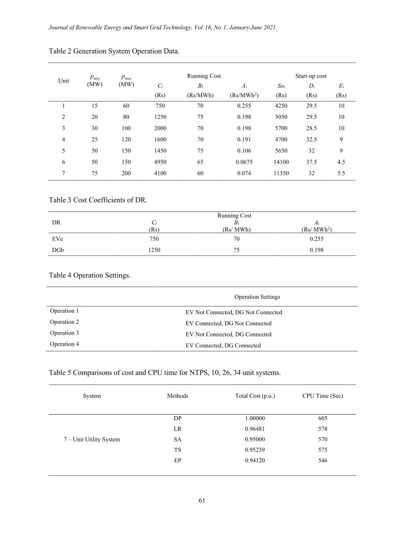
Table 2 Generation System Operation Data.

Unit

Pmin (MW)

Pmax (MW)

Running Cost

Start-up cost

Ci

(Rs)

BI

(Rs/MWh)

Ai

(Rs/MWh2)

Soi

(Rs)

Di

(Rs)

Ei

(Rs)

1 15 60 750 70 0.255 4250 29.5 10

2 20 80 1250 75 0.198 5050 29.5 10

3 30 100 2000 70 0.198 5700 28.5 10

4 25 120 1600 70 0.191 4700 32.5 9

5 50 150 1450 75 0.106 5650 32 9

6 50 150 4950 65 0.0675 14100 37.5 4.5

7 75 200 4100 60 0.074 11350 32 5.5

Table 3 Cost Coefficients of DR.

DR

Running Cost

Ci

(Rs)

Bi

(Rs/ MWh)

Ai

(Rs/ MWh2)

EVe 750 70 0.255

DGb 1250 75 0.198

Table 4 Operation Settings.

Operation Settings

Operation 1 EV Not Connected, DG Not Connected

Operation 2 EV Connected, DG Not Connected

Operation 3 EV Not Connected, DG Connected

Operation 4 EV Connected, DG Connected

Table 5 Comparisons of cost and CPU time for NTPS, 10, 26, 34 unit systems.

System Methods Total Cost (p.u.)

CPU Time (Sec)

7 – Unit Utility System

DP

LR

SA

TS

EP

1.00000

0.96481

0.95000

0.95239

0.94120

605

578

570

575

546


62

System Methods Total Cost (p.u.)

CPU Time (Sec)

10 – Unit IEEE System

DP [1]

LR [6]

SA [17]

TS [18]

EP

1.00000

0.94123

0.93210

0.93435

0.92336

325

279

285

290

254


DP [1]

LR [6]

SA [17]

TS [18]

EP

1.00000

0.95968

0.94570

0.94750

0.93680

509

495

489

494

478


DP [1]

LR [6]

SA [17]

TS [18]

EP

1.00000

0.99910

0.98015

0.98291

0.97210

1452

1368

1370

1376

1362

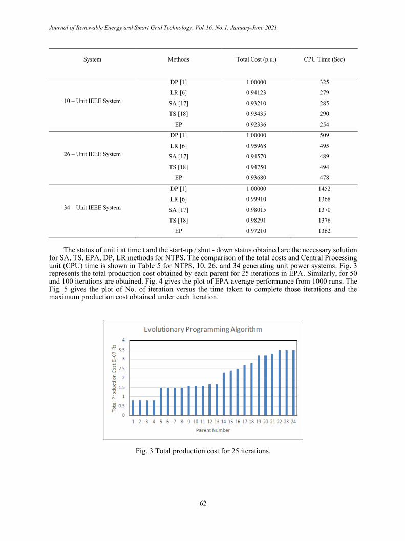
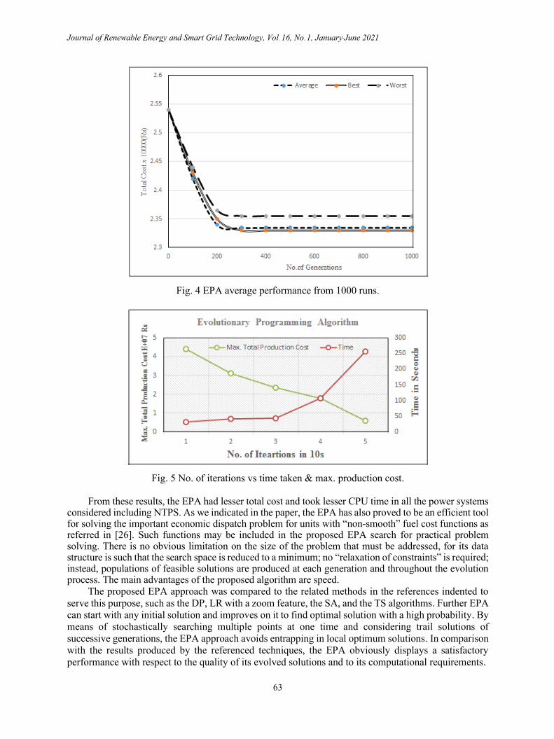
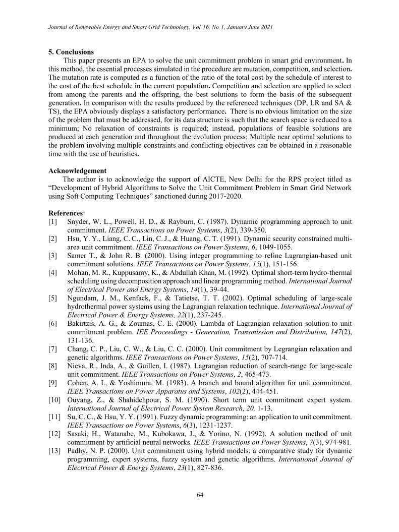
The status of unit i at time t and the start-up / shut - down status obtained are the necessary solution for SA, TS, EPA, DP, LR methods for NTPS. The comparison of the total costs and Central Processing unit (CPU) time is shown in Table 5 for NTPS, 10, 26, and 34 generating unit power systems. Fig. 3 represents the total production cost obtained by each parent for 25 iterations in EPA. Similarly, for 50 and 100 iterations are obtained. Fig. 4 gives the plot of EPA average performance from 1000 runs. The Fig. 5 gives the plot of No. of iteration versus the time taken to complete those iterations and the maximum production cost obtained under each iteration.

Fig. 3 Total production cost for 25 iterations.


63

Fig. 4 EPA average performance from 1000 runs.

Fig. 5 No. of iterations vs time taken & max. production cost.

From these results, the EPA had lesser total cost and took lesser CPU time in all the power systems

considered including NTPS. As we indicated in the paper, the EPA has also proved to be an efficient tool for solving the important economic dispatch problem for units with “non-smooth” fuel cost functions as referred in [26]. Such functions may be included in the proposed EPA search for practical problem solving. There is no obvious limitation on the size of the problem that must be addressed, for its data structure is such that the search space is reduced to a minimum; no “relaxation of constraints” is required; instead, populations of feasible solutions are produced at each generation and throughout the evolution process. The main advantages of the proposed algorithm are speed.

The proposed EPA approach was compared to the related methods in the references indented to

serve this purpose, such as the DP, LR with a zoom feature, the SA, and the TS algorithms. Further EPA

can start with any initial solution and improves on it to find optimal solution with a high probability. By

means of stochastically searching multiple points at one time and considering trail solutions of

successive generations, the EPA approach avoids entrapping in local optimum solutions. In comparison

with the results produced by the referenced techniques, the EPA obviously displays a satisfactory

performance with respect to the quality of its evolved solutions and to its computational requirements.


64

5. Conclusions

This paper presents an EPA to solve the unit commitment problem in smart grid environment. In

this method, the essential processes simulated in the procedure are mutation, competition, and selection.

The mutation rate is computed as a function of the ratio of the total cost by the schedule of interest to

the cost of the best schedule in the current population. Competition and selection are applied to select

from among the parents and the offspring, the best solutions to form the basis of the subsequent

generation. In comparison with the results produced by the referenced techniques (DP, LR and SA &

TS), the EPA obviously displays a satisfactory performance. There is no obvious limitation on the size

of the problem that must be addressed, for its data structure is such that the search space is reduced to a

minimum; No relaxation of constraints is required; instead, populations of feasible solutions are

produced at each generation and throughout the evolution process; Multiple near optimal solutions to

the problem involving multiple constraints and conflicting objectives can be obtained in a reasonable

time with the use of heuristics.

Acknowledgement

The author is to acknowledge the support of AICTE, New Delhi for the RPS project titled as

“Development of Hybrid Algorithms to Solve the Unit Commitment Problem in Smart Grid Network

using Soft Computing Techniques” sanctioned during 2017-2020.

References

[1] Snyder, W. L., Powell, H. D., & Rayburn, C. (1987). Dynamic programming approach to unit

commitment. IEEE Transactions on Power Systems, 3(2), 339-350.

[2] Hsu, Y. Y., Liang, C. C., Lin, C. J., & Huang, C. T. (1991). Dynamic security constrained multi-

area unit commitment. IEEE Transactions on Power Systems, 6, 1049-1055.

[3] Samer T., & John R. B. (2000). Using integer programming to refine Lagrangian-based unit

commitment solutions. IEEE Transactions on Power Systems, 15(1), 151-156.

[4] Mohan, M. R., Kuppusamy, K., & Abdullah Khan, M. (1992). Optimal short-term hydro-thermal

scheduling using decomposition approach and linear programming method. International Journal

of Electrical Power and Energy Systems, 14(1), 39-44.

[5] Ngundam, J. M., Kenfack, F., & Tatietse, T. T. (2002). Optimal scheduling of large-scale

hydrothermal power systems using the Lagrangian relaxation technique. International Journal of

Electrical Power & Energy Systems, 22(1), 237-245.

[6] Bakirtzis, A. G., & Zoumas, C. E. (2000). Lambda of Lagrangian relaxation solution to unit

commitment problem. IEE Proceedings - Generation, Transmission and Distribution, 147(2),

131-136.

[7] Chang, C. P., Liu, C. W., & Liu, C. C. (2000). Unit commitment by Legrangian relaxation and

genetic algorithms. IEEE Transactions on Power Systems, 15(2), 707-714.

[8] Nieva, R., Inda, A., & Guillen, I. (1987). Lagrangian reduction of search-range for large-scale

unit commitment. IEEE Transactions on Power Systems, 2, 465-473.

[9] Cohen, A. I., & Yoshimura, M. (1983). A branch and bound algorithm for unit commitment.

IEEE Transactions on Power Apparatus and Systems, 102(2), 444-451.

[10] Ouyang, Z., & Shahidehpour, S. M. (1990). Short term unit commitment expert system.

International Journal of Electrical Power System Research, 20, 1-13.

[11] Su, C. C., & Hsu, Y. Y. (1991). Fuzzy dynamic programming: an application to unit commitment.

IEEE Transactions on Power Systems, 6(3), 1231-1237.

[12] Sasaki, H., Watanabe, M., Kubokawa, J., & Yorino, N. (1992). A solution method of unit

commitment by artificial neural networks. IEEE Transactions on Power Systems, 7(3), 974-981.

[13] Padhy, N. P. (2000). Unit commitment using hybrid models: a comparative study for dynamic

programming, expert systems, fuzzy system and genetic algorithms. International Journal of

Electrical Power & Energy Systems, 23(1), 827-836.


65

[14] Zhuang, F., & Galiana, F. D. (1990). Unit commitment by simulated annealing. IEEE

Transactions on Power Systems, 5(1), 311-318.

[15] Kirkpatrick, S., Gelatt, C. D., & Vecehi, M. P. (1983). Optimisation by simulated annealing.

Science, 220, 671-680.

[16] Shokri, Z., Selim, & Alsultan, K. (1991). A simulated annealing algorithm for the clustering

problem. Pattern Recognition, 24(10), 1003-1008.

[17] Mantawy, A. H., Abdel-Magid, Y. L. & Selim, S. Z. (1998). A simulated annealing algorithm for

unit commitment. IEEE Transactions on Power Systems, 13(1), 197-204.

[18] Mantawy, A. H., Abdel-Magid, Y. L. & Selim, S. Z. (1998). A unit commitment by Tabu Search.

IEE Proceedings - Generation, Transmission and Distribution, 145(1), 56-64.

[19] Lin, W. M., Cheng, F. S., & Tsay, M. T. (2002). An improved tabu search for economic dispatch

with multiple minima. IEEE Transactions on Power Systems, 17(1), 108-112.

[20] Bai, X., & Shahidehpour, M. (1996). Hydro-thermal scheduling by tabu search and

decomposition method. IEEE Transactions on Power Systems, 11(2), 968-975.

[21] Wu, Y. G., Ho, C. Y., & Wang, D. Y. (2000). A diploid genetic approach to short-term Scheduling

of hydro-thermal system. IEEE Transactions on Power Systems, 15(4), 1268-1274.

[22] Hong, Y. Y., & Li, C. Y. (2002). Genetic algorithm based economic dispatch for cogeneration

units considering multiplant multibuyer wheeling. IEEE Transactions on Power Systems, 17(1),

134-140.

[23] Mantawy, A. H., Abdel-Magid, Y. L. & Selim, S. Z. (1999). Integrating Genetic Algorithm, Tabu

Search and Simulated Annealing For the Unit Commitment Problem. IEEE Transactions on

Power Systems, 14(3), 829-836.

[24] Wong, K. P., & Wong, Y. W. (1996). Combined genetic algorithm / simulated annealing / fuzzy

set approach to short-term generation scheduling with take-or-pay fuel contract. IEEE

Transactions on Power Systems, 11(1), 128-135.

[25] Juste, K. A., Kita, H., Tanaka, E., & Hasegawa, J. (1999). An evolutionary programming solution

to the unit commitment problem. IEEE Transactions on Power Systems, 14(4), 1452-1459.

[26] Yang, H. T., Yang, P. C., & Huang, C. L. (1996). Evolutionary programming based economic

dispatch for units with non-smooth fuel cost functions. IEEE Transactions on Power Systems,

11(1), 112-117.

[27] Wood, A. J. & Woolenberg, B. F. (1996). Power Generation and control (2nd Edn). New York,

USA: John Wiley and Sons.

[28] Lu, L., Wen, F., Xue, Y., & Xin, J. (2011). Unit commitment in power systems with plug-in

electric vehicles. Dianli Xitong Zidonghua/Automation of Electric Power Systems, 35, 16–20.

[29] Khodayar, M. E., Wu, L., & Shahidehpour, M. (2012). Hourly coordination of electric vehicle

operation and volatile wind power generation in SCUC. IEEE Transactions on Smart Grid, 3(3),

1271–1279.

[30] Ikeda, Y., Ikegami, T., Kataoka, K. & Ogimoto, K. (2012, July 22-26). A unit commitment model

with demand response for the integration of renewable energies. 2012 IEEE Power and Energy

Society General Meeting, San Diego, CA, USA.

[31] Du, P., & Lu, N. (2011). Appliance commitment for household load scheduling. Appliance

commitment for household load scheduling, 2(2), 411–419.

[32] Moghimi, H., Ahmadi, A., Aghaei, J., & Rabiee, A. (2013). Stochastic techno economic operation

of power systems in the presence of distributed energy resources. International Journal of

Electrical Power & Energy Systems, 45, 477–488.

[33] Goleijani, S., Ghanbarzadeh, T., Nikoo, F. S., &. Moghaddam, M. P. (2013). Reliability

constrained unit commitment in smart grid environment. Electric Power Systems Research, 97,

100–108.

an evolutionary programming algorithm for solving unit

Documents