solving a multiobjective possibilistic problem through compromise programming

European Journal of Operational Research 164 (2005) 748–759

www.elsevier.com/locate/dsw

Decision Aiding

Solving a multiobjective possibilistic problemthrough compromise programming q

M. Arenas Parra, A. Bilbao Terol, B. P�erez Gladish, M.V. Rodr�ıguez Ur�ıa *

Dpto. Economia Cuantitativa, Facultad de Ciencias Econ�omicas y Empresariales, Avda. del Cristo s/n,

University of Oviedo, Oviedo, Spain

Received 30 September 2002; accepted 28 November 2003

Available online 12 March 2004

Abstract

Real decision problems usually consider several objectives that have parameters which are often given by the

decision maker in an imprecise way. It is possible to handle these kinds of problems through multiple criteria models in

terms of possibility theory.

Here we propose a method for solving these kinds of models through a fuzzy compromise programming approach.

To formulate a fuzzy compromise programming problem from a possibilistic multiobjective linear programming

problem the fuzzy ideal solution concept is introduced. This concept is based on soft preference and indifference

relationships and on canonical representation of fuzzy numbers by means of their a-cuts. The accuracy between the

ideal solution and the objective values is evaluated handling the fuzzy parameters through their expected intervals and a

definition of discrepancy between intervals is introduced in our analysis.

� 2004 Elsevier B.V. All rights reserved.

Keywords: Multiple criteria decision making; Multiobjective programming; Compromise programming; Fuzzy number; Possibility

distribution; Expected interval

1. Introduction

In many complex decision situations data available may not be sufficient to define the parameters of a

real problem in an exact or objective form. It is possible to handle imprecision through the possibility

theory.

Possibility theory was proposed by Zadeh (1978) and developed by Dubois and Prade (1988); in it, fuzzy

parameters are associated with possibility distributions in the same way that random variables are

qThis work was supported by the Spanish Department of Science and Technology (project BFM2000-0010). This support is

gratefully acknowledged.* Corresponding author. Tel.: +34-8-510-2802; fax: +34-8-510-2806.

E-mail addresses: [email protected] (M. Arenas Parra), [email protected] (A. Bilbao Terol), [email protected] (B. P�erezGladish), [email protected] (M.V. Rodr�ıguez Ur�ıa).

0377-2217/$ - see front matter � 2004 Elsevier B.V. All rights reserved.

doi:10.1016/j.ejor.2003.11.028

mail to: [email protected]

M. Arenas Parra et al. / European Journal of Operational Research 164 (2005) 748–759 749

associated with probability distributions. Possibility distributions are represented as normal convex fuzzysets, such as L–R fuzzy numbers. Since the 1980s, the possibility theory has become more and more

important in the decision field and several methods have been developed to solve possibilistic programming

problems (see Buckley, 1988, 1989; Lai and Hwang, 1992; Julien, 1994; Arenas et al., 1998a,b, 1999a,b,

2001; Jim�enez et al., 2000; Saati et al., 2001).

We shall consider here a multiobjective possibilistic linear programming problem (FP-MOLP) in which

all the parameters are fuzzy. We suppose that they are represented by fuzzy numbers described by their

possibility distribution estimated by the analyst from the information supplied by the Decision Maker

(Tanaka, 1987).The uncertain and/or imprecise nature of the problem’s parameters involves two main problems: fea-

sibility and optimality. Feasibility may be handled by comparing fuzzy numbers. In this paper we use a

fuzzy relationship to compare fuzzy numbers (Jim�enez, 1996) that verifies suitable properties and that,

besides, is computationally efficient to solve linear problems because it preserves its linearity. Since this

fuzzy preference relation does not admit degrees of indifference, we have defined––in Section 2––the

concept of b-indifference.Optimality is handled through Compromise Programming (CP). CP is a well-known Multiple Criteria

Decision Making approach developed by Yu (1985) and Zeleny (1973). The basic idea in CP is the iden-tification of an ideal solution as a point where each attribute under consideration achieves its optimum

value. Zeleny states that alternatives that are closer to the ideal are preferred to those that are farther from

it because being as close as possible to the perceived ideal is the rationale of human choice.

As a natural extension of the concept of an ideal solution for a crisp multiobjective linear program-

ming problem, we are going to introduce the concept of fuzzy ideal solution. The accuracy between the

fuzzy ideal solution and the objective values is evaluated handling fuzzy parameters through their ex-

pected intervals and using some of the interval results developed in this work. In Section 3 we define the

discrepancy set and the discrepancy between intervals and also between fuzzy numbers. From these wewill transform the initial multiobjective possibilistic linear programming problem (FP-MOLP) into a

family of crisp problems.

2. Feasibility in the multiobjective possibilistic linear programming problem

We shall consider the following multiobjective possibilistic programming problem:

min ~z ¼ ð~z1;~z2; . . . ;~zkÞ ¼ ð~c1x;~c2x; . . . ;~ckxÞ

s:t: x 2 vð~A; ~bÞ ¼~aix6 ~bi; i ¼ 1; . . . ; l;

~aix ¼ ~bi; i ¼ lþ 1; . . . ;m;

xP 0;

8><>: ðFP-MOLPÞ

where xt ¼ ðx1; x2; . . . ; xnÞ is the crisp decision vector, ~ct ¼ ð~c1;~c2; . . . ;~ckÞ is composed of fuzzy vectors

which are the fuzzy coefficients of the k considered objectives, ~A ¼ ½~aij�m�n is the fuzzy technological

matrix and ~bt ¼ ð~b1; ~b2; . . . ; ~bmÞ are fuzzy parameters. We suppose that all fuzzy parameters of the

problem are given by fuzzy numbers (see Dubois and Prade, 1978, 2000) described, as we have said, by

their possibility distributions estimated by the analyst from the information supplied by the DecisionMaker.

The uncertain and/or imprecise nature of the technological matrix and of the resource vector which

defines the set of constraints of the model leads us to compare fuzzy numbers, so that the concept of b-feasibility of a decision vector has to be introduced.

750 M. Arenas Parra et al. / European Journal of Operational Research 164 (2005) 748–759

In this work we handle fuzzy numbers through their expected intervals. In particular, we are workingwith triangular fuzzy numbers. Heilpern (1992) defined the expected interval of a fuzzy triangular number~a ¼ ðaL; aC; aRÞ, as follows:

EIð~aÞ ¼ ½EIð~aÞL;EIð~aÞR� ¼ aL þ aC

2;aC þ aR

2

� �; ð1Þ

where aL is the left value, aC is the central value and aR is the right value of the fuzzy number.It can be proved that the expected interval of fuzzy numbers is a linear operator (Heilpern, 1992, the-

orem 2).

The expected interval of the fuzzy vector ~ai ¼ ð~ai1; ~ai2; . . . ; ~ainÞ is a vector whose components are the

expected intervals of each fuzzy number of vector ~ai, that is

EIð~aiÞ ¼ ðEIð~ai1Þ;EIð~ai2Þ; . . . ;EIð~ainÞÞ:
In order to compare fuzzy numbers represented by their expected intervals we use the following pref-
erence relationship:

Definition 1 (Jim�enez, 1996). For any pair of fuzzy numbers ~a and ~b the relationship of fuzzy preference

between them is defined as follows:

lMð~a; ~bÞ ¼

0 if EIð~aÞL > EIð~bÞR;EIð~bÞR � EIð~aÞL

EIð~aÞR � EIð~aÞL þ EIð~bÞR � EIð~bÞLif 0 2 ½EIð~bÞL � EIð~aÞR;EIð~bÞR � EIð~aÞL�;

1 if EIð~aÞR < EIð~bÞL;

8>>><>>>: ð2Þ

where lMð~a; ~bÞ is the degree of preference of ~a over ~b.

If lMð~a; ~bÞP b, with b 2 ½0; 1�, we say that ‘‘~a is smaller than ~b at least in a degree b’’ and it is denoted by~a6 b

~b. From Definition 1 this is equivalent to

ð1� bÞEIð~aÞL þ bEIð~aÞR 6 bEIð~bÞL þ ð1� bÞEIð~bÞR: ð3Þ

Proposition 1 (Monotony of the relationship 6 b). If 06b1 < b2 6 1 then

~a6 b2~b ) ~a6 b1

~b: ð4Þ

Definition 1 implies that if lMð~a; ~bÞ ¼ 12then the following relationships simultaneously hold: ~a6 1

2

~b and~b6 1

2~a. In this case, Jim�enez (1996) considers the fuzzy numbers ~a and ~b to be indifferent.

The previous concept implies ~a and ~b to be indifferent in an ungraduated sense, which does not allow us

to handle indifference in a flexible way. To establish flexible indifference, we define b-indifference between ~aand ~b, whose semantic would be: ‘‘lMð~a; ~bÞ is approximately 1

2’’.

Definition 2. For any pair of fuzzy numbers ~a and ~b we say that ~a is indifferent to ~b in a degree b, 06 b6 1,

denoted by ~a �b~b, if the following relationships hold simultaneously: ~a6 b

2

~b and ~b6 b2~a, i.e., ~a is indifferent

to ~b in a degree b if b26 lMð~a; ~bÞ6 1� b

2.

If b ¼ 1 then ~a and ~b are indifferent in Jim�enez’s sense.Observe that if ~a and ~b are b-indifferent then

b6 2minðlMð~a; ~bÞ; lMð~b; ~aÞÞ: ð5Þ


This b-indifference relationship verifies the following monotonicity property:

Proposition 2 (Monotony of the relationship �b). If 06 b1 < b2 6 1 then

~a �b2~b ) ~a �b1

~b: ð6Þ

Considering now the initial problem (FP-MOLP), let us introduce the following definition:

Definition 3. A decision vector x 2 IRn, is said to be b-feasible for the problem FP-MOLP if x verifies the

constraints at least in a degree b. That is

~aix6 b~bi; i ¼ 1; . . . ; l;

~aix �b~bi; i ¼ lþ 1; . . . ;m:

ð7Þ

The set of all b-feasible decision vectors is denoted by vðbÞ. From Propositions 1 and 2 the following

property immediately follows:

b1 < b2 ) vðb1Þ � vðb2Þ: ð8Þ
Observe that if the feasibility degree of each constraint is b, then 1� b is the maximum degree of
constraints unfeasibility.

According to the above considerations we shall solve the FP-MOLP through a family of problems b-FP-MOLP, 06 b6 1:


s:t: x 2 vðbÞ ¼x 2 IRn=~aix6 b

~bi; i ¼ 1; . . . ; l;

~aix �b~bi; i ¼ lþ 1; . . . ;m;

xP 0:

8><>: ðb-FP-MOLPÞ

Taking into account (3) this problem is equivalent to


s:t:

ð1� bÞEIð~aiÞL þ bEIð~aiÞRh i

x6 bEIð~biÞL þ ð1� bÞEIð~biÞR; i ¼ 1; . . . ; l;

1� b2

� �EIð~aiÞL þ b

2EIð~aiÞR

h ix6 b

2EIð~biÞL þ 1� b

2

� �EIð~biÞR; i ¼ lþ 1; . . . ;m;

b2EIð~aiÞL þ 1� b

2

� �EIð~aiÞR

h ixP 1� b

2

� �EIð~biÞL þ b

2EIð~biÞR; i ¼ lþ 1; . . . ;m;

xP 0:

9>>>>>>=>>>>>>;¼ vðbÞ:

The optimality of the initial problem is evaluated using CP and handling the fuzzy objectives, ~zr ¼ ~crx,through their expected intervals. In the next section we are going to introduce the concept of b-fuzzy ideal

solution and the discrepancy between fuzzy numbers. From these we will transform the initial FP-MOLP

into a crisp one.

3. Optimality in the multiobjective possibilistic linear programming problem

In order to apply the CP approach to solve the problem, we need to obtain the fuzzy ideal solution of b-FP-MOLP problem. For this, it is necessary to solve the following mono-objective fuzzy linear pro-

gramming problems:


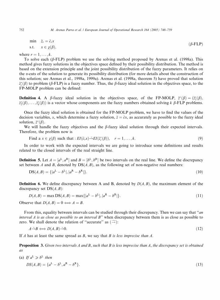
min ~zr ¼ ~crx

s:t: x 2 vðbÞ;ðb-FLPÞ

where r ¼ 1; . . . ; k.To solve each (b-FLP) problem we use the solving method proposed by Arenas et al. (1998a). This

method gives fuzzy solutions in the objectives space defined by their possibility distribution. The method isbased on the extension principle and the joint possibility distribution of the fuzzy parameters. It relies on

the a-cuts of the solution to generate its possibility distribution (for more details about the construction of

this solution; see Arenas et al., 1998a, 1999a). Arenas et al. (1998a, theorem 5) have proved that solution

~z�r ðbÞ to problem (b-FLP) is a fuzzy number. Thus, the b-fuzzy ideal solution in the objectives space, to the

FP-MOLP problem can be defined:

Definition 4. A b-fuzzy ideal solution in the objectives space, of the FP-MOLP, ~z�ðbÞ ¼ ð~z�1ðbÞ;~z�2ðbÞ; . . . ;~z�kðbÞÞ is a vector whose components are the fuzzy numbers obtained solving k b-FLP problems.

Once the fuzzy ideal solution is obtained for the FP-MOLP problem, we have to find the values of the

decision variables, x, which determine a fuzzy solution, ~z ¼ ~cx, as accurately as possible to the fuzzy ideal

solution, ~z�ðbÞ.We will handle the fuzzy objectives and the b-fuzzy ideal solution through their expected intervals.

Therefore, the problem now is

Find a x 2 vðbÞ such that : EIð~crxÞ ~!EIð~z�r ðbÞÞ; r ¼ 1; . . . ; k: ð9Þ
In order to work with the expected intervals we are going to introduce some definitions and results
related to the closed intervals of the real straight line.

Definition 5. Let A ¼ ½aL; aR� and B ¼ ½bL; bR� be two intervals on the real line. We define the discrepancy

set between A and B, denoted by DSðA;BÞ, as the following set of non-negative real numbers:

DSðA;BÞ ¼ fjaL � bLj; jaR � bRjg: ð10Þ

Definition 6. We define discrepancy between A and B, denoted by DðA;BÞ, the maximum element of the

discrepancy set DSðA;BÞ:
DðA;BÞ ¼ maxDSðA;BÞ ¼ maxfjaL � bLj; jaR � bRjg: ð11Þ
Observe that DðA;BÞ ¼ 0 () A ¼ B.

From this, equality between intervals can be studied through their discrepancy. Then we can say that ‘‘an

interval A is as close as possible to an interval B’’ when discrepancy between them is as close as possible tozero. We shall denote the relation of ‘‘accurate’’ as ðf!Þ:

A ~!B () DðA;BÞ ~!0: ð12Þ
If A has at least the same spread as B, we say that B is less imprecise than A.
Proposition 3. Given two intervals A and B, such that B is less imprecise than A, the discrepancy set is obtainedas

(a) If aL P bL then

DSðA;BÞ ¼ faL � bL; aR � bRg: ð13Þ


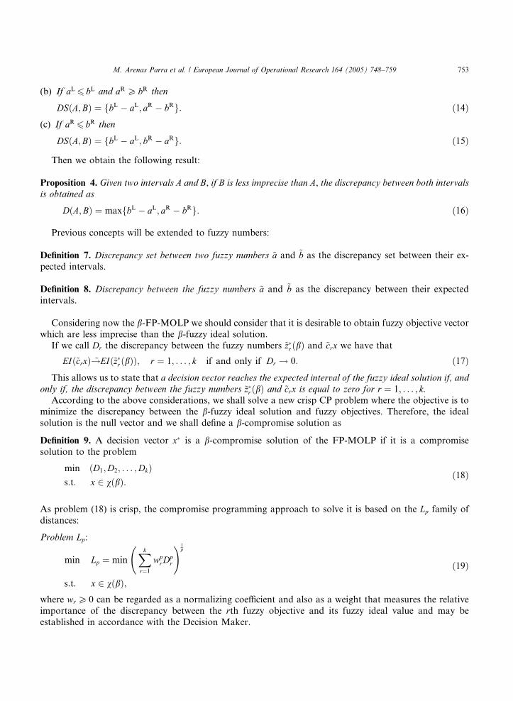
(b) If aL 6 bL and aR P bR then

DSðA;BÞ ¼ fbL � aL; aR � bRg: ð14Þ(c) If aR 6 bR then

DSðA;BÞ ¼ fbL � aL; bR � aRg: ð15Þ

Then we obtain the following result:

Proposition 4. Given two intervals A and B, if B is less imprecise than A, the discrepancy between both intervalsis obtained as

DðA;BÞ ¼ maxfbL � aL; aR � bRg: ð16Þ

Previous concepts will be extended to fuzzy numbers:

Definition 7. Discrepancy set between two fuzzy numbers ~a and ~b as the discrepancy set between their ex-

pected intervals.

Definition 8. Discrepancy between the fuzzy numbers ~a and ~b as the discrepancy between their expected

intervals.

Considering now the b-FP-MOLP we should consider that it is desirable to obtain fuzzy objective vectorwhich are less imprecise than the b-fuzzy ideal solution.

If we call Dr the discrepancy between the fuzzy numbers ~z�r ðbÞ and ~crx we have that

EIð~crxÞ ~!EIð~z�r ðbÞÞ; r ¼ 1; . . . ; k if and only if Dr ! 0: ð17Þ
This allows us to state that a decision vector reaches the expected interval of the fuzzy ideal solution if, and
only if, the discrepancy between the fuzzy numbers ~z�r ðbÞ and ~crx is equal to zero for r ¼ 1; . . . ; k.According to the above considerations, we shall solve a new crisp CP problem where the objective is to

minimize the discrepancy between the b-fuzzy ideal solution and fuzzy objectives. Therefore, the ideal

solution is the null vector and we shall define a b-compromise solution as

Definition 9. A decision vector x� is a b-compromise solution of the FP-MOLP if it is a compromise

solution to the problem

min ðD1;D2; . . . ;DkÞs:t: x 2 vðbÞ:

ð18Þ

As problem (18) is crisp, the compromise programming approach to solve it is based on the Lp family of

distances:

Problem Lp:

min Lp ¼ minXkr¼1

wprD

pr

!1p

s:t: x 2 vðbÞ;

ð19Þ

where wr P 0 can be regarded as a normalizing coefficient and also as a weight that measures the relative

importance of the discrepancy between the rth fuzzy objective and its fuzzy ideal value and may be

established in accordance with the Decision Maker.


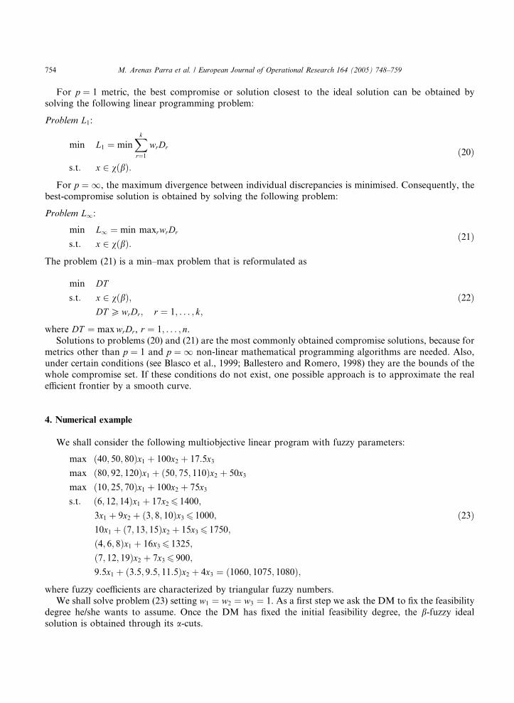
For p ¼ 1 metric, the best compromise or solution closest to the ideal solution can be obtained bysolving the following linear programming problem:

Problem L1:

min L1 ¼ minXkr¼1

wrDr

s:t: x 2 vðbÞ:ð20Þ

For p ¼ 1, the maximum divergence between individual discrepancies is minimised. Consequently, the

best-compromise solution is obtained by solving the following problem:

Problem L1:

min L1 ¼ min maxrwrDr

s:t: x 2 vðbÞ:ð21Þ

The problem (21) is a min–max problem that is reformulated as

min DT

s:t: x 2 vðbÞ;DT PwrDr; r ¼ 1; . . . ; k;

ð22Þ

where DT ¼ maxwrDr, r ¼ 1; . . . ; n.Solutions to problems (20) and (21) are the most commonly obtained compromise solutions, because for

metrics other than p ¼ 1 and p ¼ 1 non-linear mathematical programming algorithms are needed. Also,

under certain conditions (see Blasco et al., 1999; Ballestero and Romero, 1998) they are the bounds of the

whole compromise set. If these conditions do not exist, one possible approach is to approximate the real

efficient frontier by a smooth curve.

4. Numerical example

We shall consider the following multiobjective linear program with fuzzy parameters:

max ð40; 50; 80Þx1 þ 100x2 þ 17:5x3max ð80; 92; 120Þx1 þ ð50; 75; 110Þx2 þ 50x3max ð10; 25; 70Þx1 þ 100x2 þ 75x3s:t: ð6; 12; 14Þx1 þ 17x2 6 1400;

3x1 þ 9x2 þ ð3; 8; 10Þx3 6 1000;

10x1 þ ð7; 13; 15Þx2 þ 15x3 6 1750;

ð4; 6; 8Þx1 þ 16x3 6 1325;

ð7; 12; 19Þx2 þ 7x3 6 900;

9:5x1 þ ð3:5; 9:5; 11:5Þx2 þ 4x3 ¼ ð1060; 1075; 1080Þ;

ð23Þ

where fuzzy coefficients are characterized by triangular fuzzy numbers.We shall solve problem (23) setting w1 ¼ w2 ¼ w3 ¼ 1. As a first step we ask the DM to fix the feasibility

degree he/she wants to assume. Once the DM has fixed the initial feasibility degree, the b-fuzzy ideal

solution is obtained through its a-cuts.


If Dr ¼ maxðjEIð~crxÞL � EIð~z�r ÞLj, jEIð~z�r Þ

R � EIð~crxÞRjÞ and DT ¼ max Dr for r ¼ 1; 2; 3, for each fea-sibility degree b fixed by the Decision Maker, b-compromise solutions can be obtained solving the following

problems:

b-Compromise solution L1

min D1 þ D2 þ D3 þ d1 þ d2 þ d3

s:t:

45x1 þ 100x2 þ 17:5x3 � EIð~z�1ÞL � D1 6Md1;

�45x1 � 100x2 � 17:5x3 þ EIð~z�1ÞL � D1 6Mð1� d1Þ;

86x1 þ 62:5x2 þ 50x3 � EIð~z�2ÞL � D2 6Md2;

�86x1 � 62:5x2 � 50x3 þ EIð~z�2ÞL � D2 6Mð1� d2Þ;

17:5x1 þ 100x2 þ 75x3 � EIð~z�3ÞL � D3 6Md3;

�17:5x1 � 100x2 � 75x3 þ EIð~z�3ÞL � D3 6Mð1� d3Þ;

EIð~z�1ÞR � 65x1 � 100x2 � 17:5x3 � D1 6Md1;

�EIð~z�1ÞR þ 65x1 þ 100x2 þ 17:5x3 � D1 6Mð1� d1Þ;

EIð~z�2ÞR � 106x1 � 92:5x2 � 50x3 � D2 6Md2;

�EIð~z�2ÞR þ 1062x1 þ 92:5x2 þ 50x3 � D2 6Mð1� d2Þ;

EIð~z�3ÞR � 47:5x1 � 100x2 � 75x3 � D3 6Md3;

�EIð~z�3ÞR þ 47:5x1 þ 100x2 þ 75x3 � D3 6Mð1� d3Þ;

20x1 6 ðEIð~z�1ÞR � EIð~z�1Þ

LÞ þMd1

20x1 þMð1� d1ÞP ðEIð~z�1ÞR � EIð~z�1Þ

LÞ

20x1 þ 30x2ðEIð~z�2ÞR � EIð~z�2Þ

LÞ þMd2

20x1 þ 30x2 þMð1� d2ÞP ðEIð~z�2ÞR � EIð~z�2Þ

LÞ

30x1 6 ðEIð~z�3ÞR � EIð~z�3Þ

LÞ þMd3

30x1 þMð1� d3ÞP ðEIð~z�3ÞR � EIð~z�3Þ

LÞð13bþ ð1� bÞ9Þx1 þ 17x2 6 1400

9>>>>>>>>>>>>>>>=>>>>>>>>>>>>>>>;

ð1Þ

3x1 þ 9x2 þ ð9bþ ð1� bÞ5:5Þx3 6 1000

10x1 þ ð14bþ ð1� bÞ10Þx2 þ 15x3 6 1750

ð7bþ ð1� bÞ5Þx1 þ 16x3 6 1325

ð15:5bþ ð1� bÞ9:5Þx2 þ 7x3 6 900

9:5x1 þ 10:5 b2þ 1� b

2

� �6:5

� �x2 þ 4x3 6 1077:5 1� b

2

� �þ b

21067:5

9:5x1 þ 10:5 1� b2

� �þ b

26:5

� �x2 þ 4x3 P 1077:5 b

2þ 1� b

2

� �1067:5

xi P 0; i ¼ 1; 2; 3; dk 2 f0; 1g; k ¼ 1; 2; 3

9>>>>>>>>>>>>>=>>>>>>>>>>>>>;ð2Þ


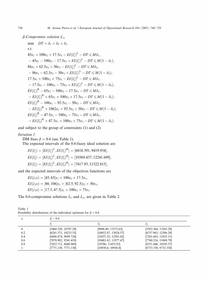
b-Compromise solution L1

Table

Possib

a

0

0.2

0.4

0.6

0.8

1

min DT þ d1 þ d2 þ d3s:t:

45x1 þ 100x2 þ 17:5x3 � EIð~z�1ÞL � DT 6Md1;

� 45x1 � 100x2 � 17:5x3 þ EIð~z�1ÞL � DT 6Mð1� d1Þ;

86x1 þ 62:5x2 þ 50x3 � EIð~z�2ÞL � DT 6Md2;

� 86x1 � 62:5x2 � 50x3 þ EIð~z�2ÞL � DT 6Mð1� d2Þ;

17:5x1 þ 100x2 þ 75x3 � EIð~z�3ÞL � DT 6Md3;

� 17:5x1 � 100x2 � 75x3 þ EIð~z�3ÞL � DT 6Mð1� d3Þ;

EIð~z�1ÞR � 65x1 � 100x2 � 17:5x3 � DT 6Md1;

� EIð~z�1ÞR þ 65x1 þ 100x2 þ 17:5x3 � DT 6Mð1� d1Þ;

EIð~z�2ÞR � 106x1 � 92:5x2 � 50x3 � DT 6Md2;

� EIð~z�2ÞR þ 1062x1 þ 92:5x2 þ 50x3 � DT 6Mð1� d2Þ;

EIð~z�3ÞR � 47:5x1 � 100x2 � 75x3 � DT 6Md3;

� EIð~z�3ÞR þ 47:5x1 þ 100x2 þ 75x3 � DT 6Mð1� d3Þ

and subject to the group of constraints (1) and (2).

Iteration 1

DM fixes b ¼ 0:6 (see Table 1).

The expected intervals of the 0.6-fuzzy ideal solution are

EIð~z�1Þ ¼ ½EIð~z�1ÞL;EIð~z�1Þ

R� ¼ ½6818:391; 9419:934�;


R� ¼ ½10369:437; 12241:699�;


R� ¼ ½7417:93; 11322:815�;

and the expected intervals of the objectives functions are

EIð~c1xÞ ¼ ½45; 65�x1 þ 100x2 þ 17:5x3;

EIð~c2xÞ ¼ ½86; 106�x1 þ ½62:5; 92:5�x2 þ 50x3;

EIð~c3xÞ ¼ ½17:5; 47:5�x1 þ 100x2 þ 75x3:

The 0.6-compromise solutions L1 and L1 are given in Table 2.

1

ility distributions of the individual optimum for b ¼ 0:6

b ¼ 0:6

~z�1 ~z�2 ~z�3

[5468.520, 10797.29] [9808.49, 13572.63] [5383.364, 13265.29]

[6281.571, 10233.35] [10032.87, 13024.57] [6757.963, 12586.29]

[6686.874, 9699.724] [10257.25, 12501.02] [7261.665, 11853.11]

[7070.982, 9241.418] [10481.62, 11977.47] [7760.216, 11069.79]

[7432.712, 8640.969] [10706, 11453.92] [8251.446, 10105.57]

[7771.130, 7771.130] [10930.4, 10930.4] [8733.338, 8733.338]

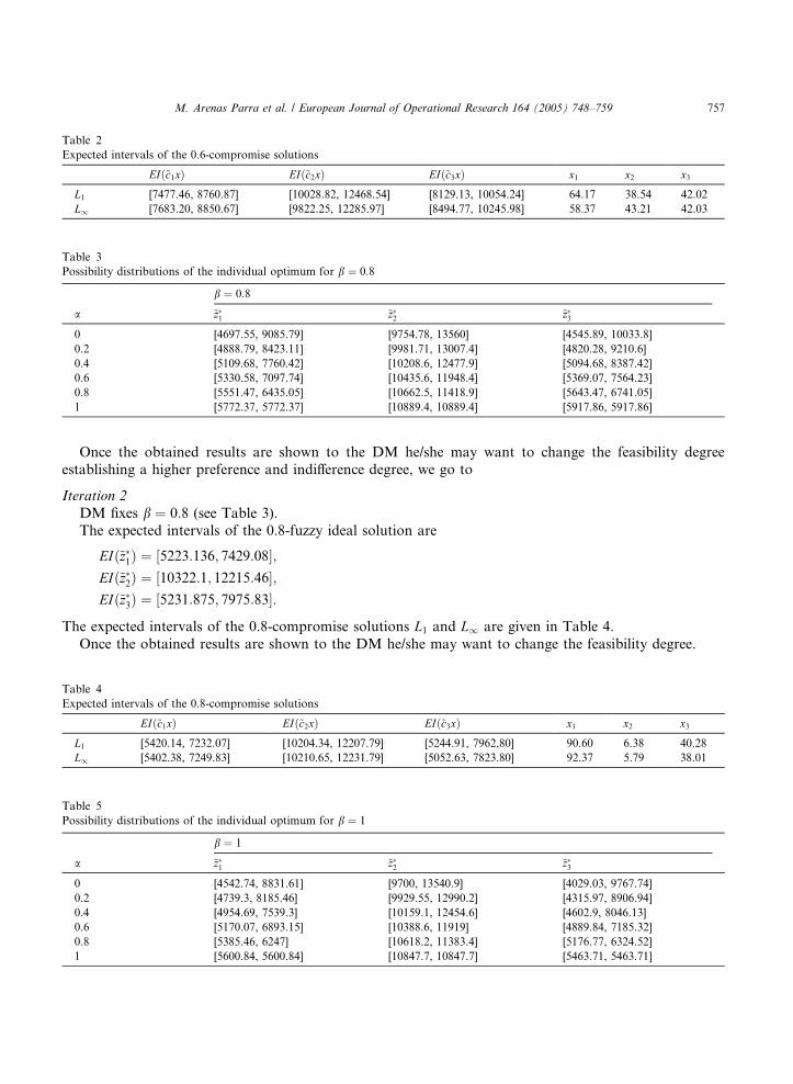
Table 2

Expected intervals of the 0.6-compromise solutions

EIð~c1xÞ EIð~c2xÞ EIð~c3xÞ x1 x2 x3

L1 [7477.46, 8760.87] [10028.82, 12468.54] [8129.13, 10054.24] 64.17 38.54 42.02

L1 [7683.20, 8850.67] [9822.25, 12285.97] [8494.77, 10245.98] 58.37 43.21 42.03

Table 3

Possibility distributions of the individual optimum for b ¼ 0:8

b ¼ 0:8

a ~z�1 ~z�2 ~z�3

0 [4697.55, 9085.79] [9754.78, 13560] [4545.89, 10033.8]

0.2 [4888.79, 8423.11] [9981.71, 13007.4] [4820.28, 9210.6]

0.4 [5109.68, 7760.42] [10208.6, 12477.9] [5094.68, 8387.42]

0.6 [5330.58, 7097.74] [10435.6, 11948.4] [5369.07, 7564.23]

0.8 [5551.47, 6435.05] [10662.5, 11418.9] [5643.47, 6741.05]

1 [5772.37, 5772.37] [10889.4, 10889.4] [5917.86, 5917.86]


Once the obtained results are shown to the DM he/she may want to change the feasibility degreeestablishing a higher preference and indifference degree, we go to

Iteration 2

DM fixes b ¼ 0:8 (see Table 3).The expected intervals of the 0.8-fuzzy ideal solution are

Table

Expect

L1

L1

Table

Possib

a

0

0.2

0.4

0.6

0.8

1

EIð~z�1Þ ¼ ½5223:136; 7429:08�;EIð~z�2Þ ¼ ½10322:1; 12215:46�;EIð~z�3Þ ¼ ½5231:875; 7975:83�:

The expected intervals of the 0.8-compromise solutions L1 and L1 are given in Table 4.

Once the obtained results are shown to the DM he/she may want to change the feasibility degree.

4

ed intervals of the 0.8-compromise solutions


[5420.14, 7232.07] [10204.34, 12207.79] [5244.91, 7962,80] 90.60 6.38 40.28

[5402.38, 7249.83] [10210.65, 12231.79] [5052.63, 7823.80] 92.37 5.79 38.01

5

ility distributions of the individual optimum for b ¼ 1

b ¼ 1

~z�1 ~z�2 ~z�3

[4542.74, 8831.61] [9700, 13540.9] [4029.03, 9767.74]

[4739.3, 8185.46] [9929.55, 12990.2] [4315.97, 8906.94]

[4954.69, 7539.3] [10159.1, 12454.6] [4602.9, 8046.13]

[5170.07, 6893.15] [10388.6, 11919] [4889.84, 7185.32]

[5385.46, 6247] [10618.2, 11383.4] [5176.77, 6324.52]

[5600.84, 5600.84] [10847.7, 10847.7] [5463.71, 5463.71]

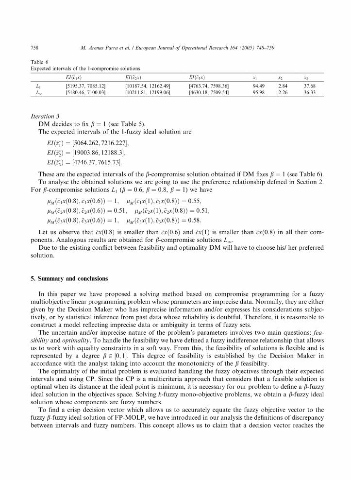
Table 6

Expected intervals of the 1-compromise solutions


L1 [5195.37, 7085.12] [10187.54, 12162.49] [4763.74, 7598.36] 94.49 2.84 37.68

L1 [5180.46, 7100.03] [10211.81, 12199.06] [4630.18, 7509.54] 95.98 2.26 36.33


Iteration 3

DM decides to fix b ¼ 1 (see Table 5).

The expected intervals of the 1-fuzzy ideal solution are

EIð~z�1Þ ¼ ½5064:262; 7216:227�;EIð~z�2Þ ¼ ½19003:86; 12188:3�;EIð~z�3Þ ¼ ½4746:37; 7615:73�:

These are the expected intervals of the b-compromise solution obtained if DM fixes b ¼ 1 (see Table 6).

To analyse the obtained solutions we are going to use the preference relationship defined in Section 2.

For b-compromise solutions L1 (b ¼ 0:6, b ¼ 0:8, b ¼ 1) we have

lMð~c1xð0:8Þ;~c1xð0:6ÞÞ ¼ 1; lMð~c1xð1Þ;~c1xð0:8ÞÞ ¼ 0:55;

lMð~c2xð0:8Þ;~c2xð0:6ÞÞ ¼ 0:51; lMð~c2xð1Þ;~c2xð0:8ÞÞ ¼ 0:51;

lMð~c3xð0:8Þ;~c3xð0:6ÞÞ ¼ 1; lMð~c3xð1Þ;~c3xð0:8ÞÞ ¼ 0:58:

Let us observe that ~cxð0:8Þ is smaller than ~cxð0:6Þ and ~cxð1Þ is smaller than ~cxð0:8Þ in all their com-

ponents. Analogous results are obtained for b-compromise solutions L1.

Due to the existing conflict between feasibility and optimality DM will have to choose his/ her preferred

solution.

5. Summary and conclusions

In this paper we have proposed a solving method based on compromise programming for a fuzzy

multiobjective linear programming problem whose parameters are imprecise data. Normally, they are either

given by the Decision Maker who has imprecise information and/or expresses his considerations subjec-

tively, or by statistical inference from past data whose reliability is doubtful. Therefore, it is reasonable toconstruct a model reflecting imprecise data or ambiguity in terms of fuzzy sets.

The uncertain and/or imprecise nature of the problem’s parameters involves two main questions: fea-sibility and optimality. To handle the feasibility we have defined a fuzzy indifference relationship that allows

us to work with equality constraints in a soft way. From this, the feasibility of solutions is flexible and is

represented by a degree b 2 ½0; 1�. This degree of feasibility is established by the Decision Maker in

accordance with the analyst taking into account the monotonicity of the b feasibility.

The optimality of the initial problem is evaluated handling the fuzzy objectives through their expected

intervals and using CP. Since the CP is a multicriteria approach that considers that a feasible solution isoptimal when its distance at the ideal point is minimum, it is necessary for our problem to define a b-fuzzyideal solution in the objectives space. Solving k-fuzzy mono-objective problems, we obtain a b-fuzzy ideal

solution whose components are fuzzy numbers.

To find a crisp decision vector which allows us to accurately equate the fuzzy objective vector to the

fuzzy b-fuzzy ideal solution of FP-MOLP, we have introduced in our analysis the definitions of discrepancy

between intervals and fuzzy numbers. This concept allows us to claim that a decision vector reaches the


expected interval of the fuzzy ideal solution if the discrepancy between the b-fuzzy ideal solution and thefuzzy objectives is equal to zero. Then we have solved a crisp CP problem.

The described solving method includes Decision Maker preferences about discrepancy weights, as well as

the degree of feasibility of the decision variables that he/she is willing to accept in each case.

Acknowledgements

We are grateful to the referees for their useful comments and suggestions.

References

Arenas, M., Bilbao, A., Jim�enez, M., Rodr�ıguez, M.V., 1998a. A theory of possibilistic approach to the solution of a fuzzy linear

programming. In: Giron, J. (Ed.), Applied Decision Analysis. Kluwer Academic Publishers.

Arenas, M., Bilbao, A., Jim�enez, M., Rodr�ıguez, M.V., 1998b. M�etodo Interactivo de Resoluci�on de un Programa Multiobjetivo

Linear Posibil�ıstico. Monogr�afico: Problemas complejos de decisi�on. Rev. R. Acad. Cien. Exact. Fis. Nat. (Esp), vol. 92, no. 4, pp.

423–428.

Arenas, M., Bilbao, A., Rodr�ıguez, M.V., 1999a. Solving the multiobjective possibilistic linear programming problem. European

Journal of Operational Research 117, 175–182.

Arenas, M., Bilbao, A., Rodr�ıguez, M.V., 1999b. Solution of a possibilistic multiobjective linear programming problem. European

Journal of Operational Research 119, 338–344.

Arenas, M., Bilbao, A., Rodr�ıguez, M.V., 2001. A fuzzy goal programming approach to portfolio selection. European Journal of

Operational Research 133, 287–297.

Ballestero, E., Romero, C., 1998. Multiple Criteria Decision Making and Its Applications to Economic Problems. Kluwer Academic

Publishers, Boston.

Blasco, E., Cuchillo-Ib�a~nez, E., Mor�on, M.A., Romero, C., 1999. On the monotonicity of the compromise set in multicriteria

problems. Journal of Optimization Theory and its Applications 102 (1), 69–82.

Buckley, J.J., 1988. Possibilistic linear programming with triangular fuzzy numbers. Fuzzy Sets and Systems 26, 135–138.

Buckley, J.J., 1989. Solving possibilistic linear programming problems. Fuzzy Sets and Systems 31, 329–341.

Dubois, D., Prade, H., 1978. Operations on fuzzy numbers. International Journal of Systems Sciences 9 (6), 613–626.

Dubois, D., Prade, H., 1988. Possibility Theory. Plenum Press, New York.

Dubois, D., Prade, H., 2000. Fundamentals of Fuzzy Sets. In: Handbooks of Fuzzy Sets Series. Kluwer Academic Publishers.

Heilpern, S., 1992. The expected value of a fuzzy number. Fuzzy Sets and Systems 47, 81–86.

Jim�enez, M., 1996. Ranking fuzzy numbers through the comparison of their expected intervals. International Journal of Uncertainty.

Fuzziness and Knowledge-Based Systems 4 (4), 379–388.

Jim�enez, M., Arenas, M., Bilbao, A., Rodr�ıguez, M.V., 2000. Solving a possibilistic linear program through compromise

programming. Mathware & Soft Computing 7 (2–3), 175–184.

Julien, B., 1994. An extension to possibilistic linear programming. Fuzzy Sets and Systems 64, 195–206.

Lai, Y.J., Hwang, C.L., 1992. A new approach to some possibilistic linear programming problem. Fuzzy Sets and Systems 49, 121–133.

Saati, M.S., Memariani, A., Jahanshahloo, G.R., 2001. a-cut Based Possibilistic Programming. In: Proceedings of the First National

Industrial Engineering Conference, Iran, pp. 1–10.

Tanaka, H., 1987. Fuzzy data analysis by possibilistic linear models. Fuzzy Sets and Systems 24, 363–375.

Yu, P.L., 1985. M�ultiple-Criteria Decisi�on Making. Concepts, Techniques and Extensions. Plenum Press, New York.

Zadeh, L.A., 1978. Fuzzy sets as a basis for a theory of possibility. Fuzzy Sets and Systems 1, 3–28.

Zeleny, M., 1973. Compromise programming. In: Cochrane, J.L., Zeleny, M. (Eds.), Multiple Criteria Decision Making. University of

South Carolina, Columbia, SC, pp. 262–301.

solving a multiobjective possibilistic problem through compromise programming

Documents