multiobjective modelling of biofuels supply systems
TRANSCRIPT
The copyright of this thesis vests in the author. No quotation from it or information derived from it is to be published without full acknowledgement of the source. The thesis is to be used for private study or non-commercial research purposes only.
Published by the University of Cape Town (UCT) in terms of the non-exclusive license granted to UCT by the author.
Univers
ity of
Cap
e Tow
n
MULTIOBJECTIVE MODELLING OF BIOFUEL SUPPLY
SYSTEMS
A thesis submitted to the
UNIVERSITY OF CAPE TOWN
In fulfilment of the requirements for the Degree of
MASTER OF SCIENCE IN ENGINEERING
(CHEMICAL ENGINEERING)
BY
THAPELO CLIFFORD MOHALE LETETE
B.Sc Mathematics & Applied Chemistry, Lesotho; B.Sc (ENG) Chemical, UCT
March 2009
Univers
ity of
Cap
e Tow
n
Thapelo Letete – Multiobjective modelling of biofuels supply systems i
"I know the meaning of plagiarism and declare that all the work in the document, save for that which is properly acknowledged, is my own"
Univers
ity of
Cap
e Tow
n
Thapelo Letete – Multiobjective modelling of biofuels supply systems ii
EXECUTIVE SUMMARY
Biomass was the world’s primary source of energy in the transportation sector until the late 1920’s when
cheap and abundant fossil fuel brought about the petroleum fuel paradigm, and bioenergy usage was
virtually abandoned. The threat of constantly depleting fossil fuel reserves and the ever-increasing
evidence of climate change associated with the use of fossil fuels have, however, sparked renewed
interest in the use of bioenergy in recent years, forcing energy planners and policy-makers to rethink its
role in the energy system for the coming years. In particular, liquid biofuels have been receiving the
most attention throughout the world for their potential to substitute conventional transportation fuels.
South Africa has also recognized the need to integrate biofuels into the national energy mix, and
consequently the government has established a National Industrial Biofuels Strategy, which sets a
national biofuel target of 2% of road liquid transport fuels for 2013. Contrary to the international
situation, the main driver for the development of a biofuels industry in South Africa is the need to create
a link between the country’s first and second economies, and this centres around the development of
agriculture and the use of currently underutilized land in those areas of the country that were previously
neglected by the apartheid regime. Because of the scarcity of arable land in South Africa, however, it is
necessary to facilitate the effective utilisation of this limited resource if sustainability and maximum
return on input are to be achieved. The aim of this thesis is to determine the optimal land use options
offered by different bioenergy crops and technologies available to South Africa for the development of
the most efficient and sustainable agriculture-based biofuels industry.
A review of relevant literature showed that biofuels are a potential low-carbon energy source, but
whether they actually offer the carbon savings depends on the location, type of feedstock and method of
production, and life-cycle assessment methods were found to be the right tools for analysing the
sustainability of biofuel supply chains. It was also found that land use change and deforestation for
biofuel production strongly influence the success and sustainability of bioenergy systems, and that their
effects should always be taken into account in analysing the environmental and social impacts of
bioenergy systems from a life-cycle perspective. The literature review further revealed that while energy
modelling can be used to analyse bioenergy systems from an economic viewpoint only and life-cycle
assessment tools can be adequately used to analyse their social and environmental aspects,
multiobjective optimization is the best method for integrated analysis of all three dimensions.
The system analysed in this thesis comprises of underutilized arable land that can be used for growing
maize, wheat, sugarcane or sweet sorghum for ethanol production, and soybean, sunflower or canola for
biodiesel production, depending on the different area suitabilities of these crops in South Africa.
Univers
ity of
Cap
e Tow
n
Thapelo Letete – Multiobjective modelling of biofuels supply systems iii
Firstly, analyses of energy balances and land use change were carried out on the respective biofuel
supply chains, and the results showed that the production of biofuels from maize grain, wheat grain,
sugarcane, sweet sorghum cane, soybean, sunflower and canola in South Africa all result in net energy
gains, with sugarcane having the highest Net Energy Balance ratio of 3.72 while maize grain had the
lowest at 1.20. The results also showed that bringing land that has not been cultivated for a period of two
years into biofuel production results in a once-off carbon debt of about 13,900 kgCO2/ha which the
biofuels can only repay if their production and use avoid the emission of greenhouse gases in each
subsequent year. Sugarcane ethanol was found to have the shortest repayment period of 3 years, while
sweet sorghum ethanol and maize grain ethanol would not be able to repay the carbon debt under the
assumptions of this thesis.
These analyses were followed by the development of a multiobjective optimization model which was
then applied to the system. The model simultaneously maximises three objectives; economic gain by the
processing plant, direct job creation in the biofuels industry and greenhouse gas emissions avoided by
using the biofuels, all at minimal use of agricultural land. The objectives were chosen as the most
prominent economic, social and environmental objectives respectively for the establishment of a
biofuels industry in South Africa. Two scenarios were investigated here; a scenario where there is no
targeted market penetration of biofuels and scenario of B2 (2% biodiesel mix with 98% diesel) and E8
(8% ethanol mix with 92% petrol) national target.
The results showed that in the absence of a market penetration target, sugarcane is the most preferable
crop for maximising all three objectives wherever it can grow throughout the country. In the Western
Cape areas where sugarcane cannot grow, canola is the most preferred for maximising avoided
greenhouse gas emissions and job creation. For maximising economic gain in these areas, however,
canola is only better than wheat but it is actually more economical to leave the land uncultivated than to
use it for growing crops for biofuels production. In the areas outside the Western Cape where sugarcane
cannot grow, sweet sorghum is the most preferred for maximizing both economic gain and job creation,
while sunflower and canola are the most preferred and second most preferred crops respectively for
maximizing avoided greenhouse gas emissions. A trade-off analysis of the objectives in the absence of a
national market target revealed that an estimated 47 kg of CO2-eqt emissions per hectare are avoided
when maximizing economic gain and job creation, but any additional kilogram of CO2-eqt emissions
avoided thereafter comes at a price of R4.50 of economic gain and 0.2 man-hours of labour.
The results of the model also showed that in the presence of the three objectives are maximized by three
distinct crop combinations; economic gain is maximized by growing as much sugarcane as possible for
ethanol production and as much canola as possible where sugarcane cannot be grown and then
supplementing them with maize and sunflower respectively to achieve the required ratio of B2 and E8.
Univers
ity of
Cap
e Tow
n
Thapelo Letete – Multiobjective modelling of biofuels supply systems iv
Job creation is maximised by the same distribution as economic gain except that sweet sorghum, instead
of maize, supplements sugarcane. Avoided greenhouse gas emissions, on the other hand, are maximized
by growing as much sugarcane as possible for ethanol production and then balancing between sunflower
for biodiesel production and wheat for ethanol production to achieve the desired proportion. The crop
combination that maximises job creation was found to produce the largest quantity of biofuels per
hectare per annum, followed by the combination that maximises economic gain.
Lastly a case study was conducted on a local municipal area of Maluti-a-Phofung to demonstrate the use
of the multiobjective optimization model to support biofuel decision-making in South Africa. This area
was chosen because it fits all the criteria of the National Industrial Biofuels Strategy of South Africa
perfectly, in terms of its history, economic situation and availability of underutilized arable land. An
analysis of the current situation in Maluti-a-phofung revealed that local economic development and
poverty eradication through job creation would be the two major objectives to be achieved by the
development of a local biofuels programme in this area, and that Integrated Development Planning
(IDP), would be the right context in which decisions about the areas’ approach in developing such a
programme would be taken.
Two scenarios were modelled in the case study; a scenario involving only the four crops familiar to the
local farmers, namely maize, wheat, soybean and sunflower (four crops scenario), and a scenario where
the farmers would be willing to include sweet sorghum in the programme (all crops scenario). A
biodiesel plant would be established in the area for biodiesel production while bioethanol crops would
be sent to the nearest processing plants outside the bounds of the municipality.
The case study results showed that, in both scenarios, growing wheat for ethanol production would
result in maximum net economic gain for the municipal area as a whole, while growing maize and sweet
sorghum would result in maximum job creation in the four crops scenario and in the all crops scenario
respectively. A trade-off analysis of the objectives showed that while the creation of 6.1 man-hours of
labour comes with maximising economic gain, any additional man-hour of labour created thereafter
would come at a loss of R11.30 and R193.00 of economic gain to the municipality in the all-crops
scenario and in the four crops scenario respectively. The Maluti-a-Phofung IDP team would then use
this information to pick the scenario and the crop combination that best represent the interests of the
people of Maluti-a-Phofung.
It was recommended that the model be broadened in future research to incorporate other objectives like
water usage and plant capital cost which can influence the choice of crops and processing technologies.
Univers
ity of
Cap
e Tow
n
Thapelo Letete – Multiobjective modelling of biofuels supply systems v
ACKNOWLEDGEMENTS
Glory be to God without whom this thesis would not have been possible!
Special thanks go to A/Professor Harro von Blottnitz for his guidance and mentorship throughout the
course of my project.
I would also like to extend my thanks to the Thabo Mofutsanyana district agricultural office and the
Maluti-a-Phofung municipal office for assisting me with data collection. Thanks also go to Bolelang
Sibolla for her assistance with interpreting mapping data, Rethabile Melamu and Dr. Andrew Marquard
for assisting me with editing and proofreading of the thesis. Finally, I would like to thank my entire
family for being there for me and motivating me throughout my studies.
This thesis is dedicated to my wife ‘Mampepuoa and our little baby girl Mpepuoa.
Univers
ity of
Cap
e Tow
n
Thapelo Letete – Multiobjective modelling of biofuels supply systems vi
TABLE OF CONTENTS
EXECUTIVE SUMMARY ........................................................................................................................ ii
ACKNOWLEDGEMENTS........................................................................................................................ v
TABLE OF CONTENTS........................................................................................................................... vi
LIST OF FIGURES ................................................................................................................................... xi
LIST OF TABLES................................................................................................................................... xiii
MODEL INPUTS .................................................................................................................................... xiv
1. INTRODUCTION .............................................................................................................................. 1
1.1. Background................................................................................................................................. 1
1.2. Problem Statement ...................................................................................................................... 3
1.3. Objectives ................................................................................................................................... 3
1.4. Key Questions............................................................................................................................. 4
1.5. Scope and Limitations................................................................................................................. 4
1.6. Thesis Outline ............................................................................................................................. 5
2. LITERATURE REVIEW ................................................................................................................... 7
2.1. Review of Bioenergy .................................................................................................................. 7
2.1.1. Bioenergy Supply Chains ................................................................................................... 7
2.1.2. The Potential of Biomass contribution to Energy............................................................... 8
2.1.3. Biofuels ............................................................................................................................... 8
2.1.3.1. Bioethanol ................................................................................................................... 9
2.1.3.2. Biodiesel ..................................................................................................................... 9
2.2. Bioenergy developments in South Africa ................................................................................. 10
2.3. Sustainability of bioenergy from a life-cycle perspective ........................................................ 15
2.3.1. Energy balancing .............................................................................................................. 16
2.3.2. Carbon balancing .............................................................................................................. 17
2.4. Concerns over biofuels ............................................................................................................. 17
2.5. Energy Modelling ..................................................................................................................... 21
2.5.1. A Review of Energy models ............................................................................................. 22
Univers
ity of
Cap
e Tow
n
Thapelo Letete – Multiobjective modelling of biofuels supply systems vii
2.5.2. Application of modelling to Bioenergy ............................................................................ 24
2.5.3. Bioenergy Modelling in South Africa............................................................................... 25
2.6. Multicriteria Decision-making in Energy Systems................................................................... 26
2.6.1. Principles of Multicriteria Decision-making .................................................................... 27
2.6.2. Multiobjective optimization solution methods ................................................................. 28
2.6.2.1. The Parameter Spacing Method................................................................................ 28
2.6.2.2. The Weighting Method............................................................................................. 29
2.6.2.3. The ε-constraint method............................................................................................ 29
2.7. Summary of the Literature Review and outlook....................................................................... 30
3. SYSTEM DESCRIPTION AND MULTICRITERIA MODELLING ............................................. 31
3.1. Adopted Methodology .............................................................................................................. 31
3.2. System Description ................................................................................................................... 31
3.2.1. Processing Technologies................................................................................................... 32
3.2.1.1. Grain processing ....................................................................................................... 32
3.2.1.2. Cane Processing........................................................................................................ 34
3.2.1.3. Oilseed Processing.................................................................................................... 34
3.2.2. Bioenergy Crops ............................................................................................................... 35
3.2.2.1. Maize......................................................................................................................... 35
3.2.2.2. Wheat ........................................................................................................................ 36
3.2.2.3. Sugarcane.................................................................................................................. 36
3.2.2.4. Sweet Sorghum ......................................................................................................... 36
3.2.2.5. Soybean..................................................................................................................... 37
3.2.2.6. Sunflower seed.......................................................................................................... 38
3.2.2.7. Canola ....................................................................................................................... 38
3.2.3. Land suitability of biofuel crops ....................................................................................... 39
3.2.4. System Boundary.............................................................................................................. 40
3.3. Allocation.................................................................................................................................. 41
3.4. Model Objectives ...................................................................................................................... 42
Univers
ity of
Cap
e Tow
n
Thapelo Letete – Multiobjective modelling of biofuels supply systems viii
3.4.1. Economic objective........................................................................................................... 42
3.4.2. Social objective................................................................................................................. 42
3.4.3. Environmental objective ................................................................................................... 43
3.5. Problem Formulation ................................................................................................................ 43
3.6. Objective Equations .................................................................................................................. 44
3.6.1. Maximisation of Economic gain....................................................................................... 44
3.6.2. Maximisation of Avoided Greenhouse gas emissions...................................................... 45
3.6.3. Maximisation of job creation............................................................................................ 48
3.7. Problem Constraints.................................................................................................................. 48
3.7.1. Crop suitability constraints ............................................................................................... 49
3.7.2. Land availability ............................................................................................................... 50
3.8. Model Formulation ................................................................................................................... 50
3.8.1. No target market penetration ............................................................................................ 50
3.8.2. B2 and E8 market penetration........................................................................................... 50
3.9. Solution Method........................................................................................................................ 51
3.10. Inventory Preparation............................................................................................................ 51
3.10.1. Inputs................................................................................................................................. 52
3.10.1.1. Seeds ......................................................................................................................... 52
3.10.1.2. Farm fossil fuel use................................................................................................... 52
3.10.1.3. Fertilizers and Agrochemicals .................................................................................. 52
3.10.1.4. Machinery and Facility construction ........................................................................ 53
3.10.1.5. Farm and biofuel labour............................................................................................ 54
3.10.1.6. Transportation ........................................................................................................... 54
3.10.1.7. Facility Energy use ................................................................................................... 55
3.10.2. Outputs.............................................................................................................................. 55
3.10.2.1. By-Product Credits.................................................................................................... 56
3.10.3. Energy coefficients and emission factors ......................................................................... 57
3.10.4. Labour requirement and Costing ...................................................................................... 59
Univers
ity of
Cap
e Tow
n
Thapelo Letete – Multiobjective modelling of biofuels supply systems ix
3.10.4.1. Labour Requirement ................................................................................................. 59
3.10.4.2. Costing ...................................................................................................................... 60
3.10.5. Land Use Change parameters ........................................................................................... 60
3.11. Conclusion ............................................................................................................................ 61
4. NATIONAL MODEL RESULTS .................................................................................................... 62
4.1. Net Energy Balances................................................................................................................. 62
4.1.1. Maize Grain Ethanol ......................................................................................................... 65
4.1.2. Wheat Grain Ethanol......................................................................................................... 65
4.1.3. Sugarcane Ethanol ............................................................................................................ 65
4.1.4. Sweet Sorghum Ethanol.................................................................................................... 66
4.1.5. Soybean Biodiesel............................................................................................................. 66
4.1.6. Sunflower Biodiesel.......................................................................................................... 67
4.1.7. Canola Biodiesel ............................................................................................................... 67
4.1.8. Conclusions....................................................................................................................... 67
4.2. Environmental effects of Land use change............................................................................... 68
4.2.1. Sensitivity analysis of the repayment periods................................................................... 71
4.2.2. Conclusions....................................................................................................................... 74
4.3. Results of Multicriteria Modelling............................................................................................ 75
4.3.1. No market penetration target ............................................................................................ 75
4.3.1.1. Price sensitivity of crop distributions – No market penetration target ..................... 81
4.3.2. B2 and E8 market penetration........................................................................................... 83
4.3.2.1. Price sensitivity of crop distributions – B2 and E8 market penetration ................... 87
4.4. Summary of key findings and outlook...................................................................................... 89
5. MALUTI-A-PHOFUNG LOCAL GOVERNMENT CASE STUDY.............................................. 91
5.1. Area Description ....................................................................................................................... 91
5.1.1. The economic situation ..................................................................................................... 93
5.1.2. The Agricultural situation................................................................................................. 94
5.1.3. Integrated Development Planning..................................................................................... 96
Univers
ity of
Cap
e Tow
n
Thapelo Letete – Multiobjective modelling of biofuels supply systems x
5.2. Biofuels in Maluti-a-phofung ................................................................................................... 97
5.2.1. Feedstock and land use ..................................................................................................... 98
5.2.2. Biofuel options for Maluti-a-Phofung .............................................................................. 99
5.2.2.1. Biodiesel-only approach ......................................................................................... 100
5.2.2.2. Bioethanol-only approach....................................................................................... 100
5.2.2.3. Biodiesel and Bioethanol approach ........................................................................ 100
5.3. The Decision Support System................................................................................................. 101
5.3.1. DSS Model Equations..................................................................................................... 101
5.3.1.1. Economic gain in Maluti-a-Phofung....................................................................... 101
5.3.1.2. Job-creation in Maluti-a-Phofung........................................................................... 103
5.3.1.3. DSS Model formulation.......................................................................................... 103
5.3.2. Case-study Inventory ...................................................................................................... 104
5.3.3. DSS Results and Discussions ......................................................................................... 104
5.3.3.1. Results of baseline scenarios .................................................................................. 104
5.3.3.2. Sensitivity analysis.................................................................................................. 108
5.3.4. Conclusions..................................................................................................................... 110
6. CONCLUSIONS AND RECOMMENDATIONS ......................................................................... 112
6.1. Responding to the key questions............................................................................................. 115
6.2. Recommendations for future work ......................................................................................... 116
7. REFERENCES ............................................................................................................................... 117
APPENDICES ........................................................................................................................................ 123 Univ
ersity
of C
ape T
own
Thapelo Letete – Multiobjective modelling of biofuels supply systems xi
LIST OF FIGURES
Figure 1. 1: Outline of thesis structure........................................................................................................ 5
Figure 2. 1: Summary of Common Bioenergy Pathways (European Biomass Association, 2009) ........... 7
Figure 2. 2: methanol-catalysed production of biodiesel............................................................................ 9
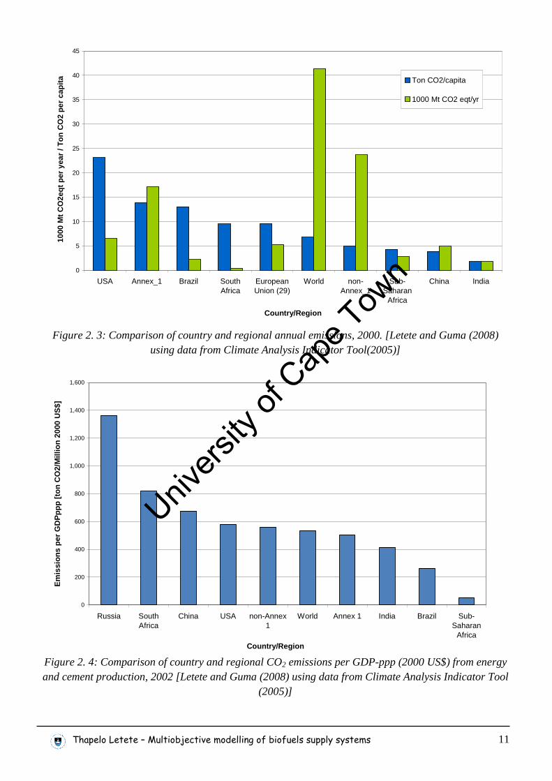
Figure 2. 3: Comparison of country and regional annual emissions, 2000. [Letete and Guma (2008) using data from Climate Analysis Indicator Tool(2005)]......................................................................... 11
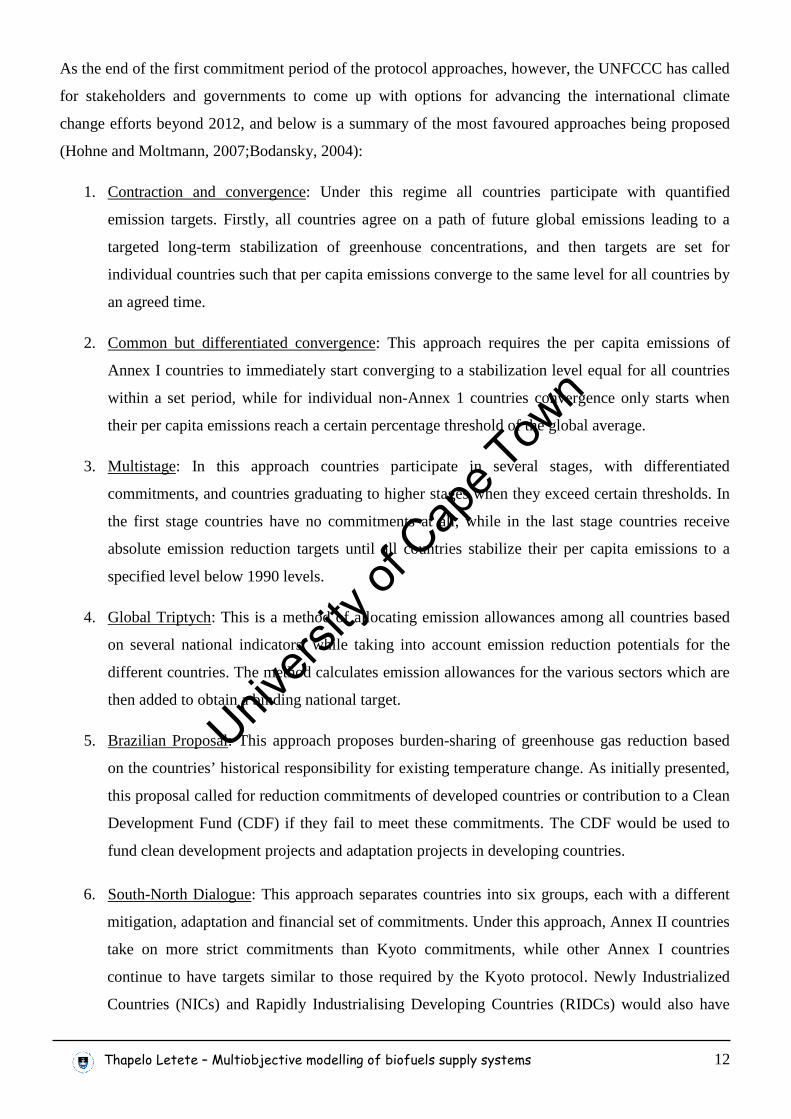
Figure 2. 4: Comparison of country and regional CO2 emissions per GDP-ppp (2000 US$) from energy and cement production, 2002 [Letete and Guma (2008) using data from Climate Analysis Indicator Tool (2005)]....................................................................................................................................................... 11
Figure 2. 5: The carbon debts for nine scenarios of converting habitats to biofuel production (Fargoine et al., 2008) ................................................................................................................................................... 19
Figure 2. 6: Comparison of of GHG reduction capacities of food-based biofuels grown on fertile soils with LIHD-based biofuels from agriculturally degraded soil (Tilman et al., 2006)................................. 21
Figure 3. 1: Biofuel supply chain network modelled in this thesis........................................................... 33
Figure 3. 2: The locations of all the bioethanol plants in the model......................................................... 34
Figure 3. 3: The crop suitability of bioenergy crops as modelled in the thesis ........................................ 40
Figure 3. 4: Greenhouse gas emissions associated with biofuel production............................................. 46
Figure 4. 1: Net Energy Balance of biofuels in South Africa................................................................... 62
Figure 4. 2: Agricultural energy inputs in biofuel production per hectare ............................................... 63
Figure 4. 3: Post-harvest energy inputs in biofuel production.................................................................. 64
Figure 4. 4: Avoided GHG emissions of biofuels produced from the different energy crops.................. 69
Figure 4. 5: Sensitivity of avoided GHG emissions to changes in crop transportation distances ............ 70
Figure 4. 6: Number of years required to repay the carbon debt. ............................................................. 71
Figure 4. 7: Sensitivity of number of repayment years to number of years land was abandoned ............ 72
Figure 4. 8: Sensitivity of repayment period to changes in crop yields.................................................... 73
Figure 4. 9: Variation of sweet sorghum repayment period with transportation distance........................ 74
Figure 4. 10: Area-based crop distribution that results in maximum economic gain and job creation – no market penetration target .......................................................................................................................... 76
Figure 4. 11: Area-based crop distribution that results in maximum avoided greenhouse gas emissions – no market penetration target ..................................................................................................................... 76
Figure 4. 12: Economic gain abilities of the different biofuels ................................................................ 77
Figure 4. 13: Job creation abilities of different biofuels........................................................................... 77
Figure 4. 14: 3-Dimensional trade-off curve (Pareto curve) for target-free market penetration .............. 78
Univers
ity of
Cap
e Tow
n
Thapelo Letete – Multiobjective modelling of biofuels supply systems xii
Figure 4. 15: 2-Dimensional trade-off curves in the absence of a market penetration target................... 79
Figure 4. 16: Variation of the trade-off curve crop distributions with avoided emissions ....................... 80
Figure 4. 17: Variation of the trade-off curve crop distributions with economic gain ............................. 80
Figure 4. 18: Variation of optimal crop distributions with changes in fuel prices and commodity prices – no market penetration target ..................................................................................................................... 82
Figure 4. 19: Area-based crop distribution resulting in maximum economic gain – B2E8 market penetration................................................................................................................................................. 83
Figure 4. 20: Area-based crop distribution resulting in the maximum job creation – B2E8 market penetration................................................................................................................................................. 84
Figure 4. 21: Area-based crop distribution that gives the maximum avoided greenhouse gas emissions – B2E8 market penetration .......................................................................................................................... 84
Figure 4. 22: Trade-off curve of the E2E8 market penetration target in 3-dimensions............................ 85
Figure 4. 23: Trade-off curve of the E2E8 market penetration target in 2-dimensions............................ 86
Figure 4. 24: Crop combinations of the trade-off curve that achieves a market penetration of B2 and E8................................................................................................................................................................... 87
Figure 4. 25: Variation of optimal crop distributions with changes in fuel prices and commodity prices – B2 and E8 market penetration................................................................................................................... 88
Figure 5. 1: Map of Maluti-a-phofung local municipality (Municipal Demarcation Board, 2008) ......... 92
Figure 5. 2: The contribution of each economic sector to GDP and employment in Maluti-a-phofung (Business Trust and DPLG, 2007) ............................................................................................................ 93
Figure 5. 3: Land-use distribution in the Maluti-a-Phofung municipality (Thabo Mofutsanyana district DoA, 2008) ............................................................................................................................................... 99
Figure 5. 4: Economic gain and job creation trade-off curve for Maluti-a-Phofung.............................. 106
Figure 5. 5: Pareto optimal crop distribution of the all-crops scenario .................................................. 107
Figure 5. 6: Pareto optimal crop distributions for the four crop scenario............................................... 107
Figure 5. 7: The effect of assumed current land-use fraction on the objectives ..................................... 108
Figure 5. 8: Sensitivity of maximum economic gain to changes in the fraction of grain currently sold as second grade............................................................................................................................................ 109
Figure 5. 9: Sensitivity of Economic-gain to changes in commodity prices .......................................... 110
Univers
ity of
Cap
e Tow
n
Thapelo Letete – Multiobjective modelling of biofuels supply systems xiii
LIST OF TABLES
Table 2. 1: Comparative energy flows in producing ethanol from switchgrass and corn (McLaughlin and Walsh, 1998)............................................................................................................................................. 20
Table 2. 2: Characteristics of top-down models and bottom-up models (Nakata, 2004) ......................... 22
Table 2. 3: Typical Energy-economic models (Becker and Barry, 2006) ................................................ 23
Table 3. 1: National Crop Suitability........................................................................................................ 39
Table 3.2: Material and Energy inputs to the system................................................................................ 41
Table 3. 3: Sources of emissions in agricultural operations ..................................................................... 47
Table 3. 4: Fertilizer and Pesticide application rates ................................................................................ 53
Table 3. 5: Energy consumption in processing plant per litre of biofuel.................................................. 55
Table 3. 6: Crop and biofuel Yields.......................................................................................................... 55
Table 3. 7: Energy and greenhouse gas emission coefficients of selected inputs..................................... 57
Table 3. 8: By-product emission factors ................................................................................................... 58
Table 3. 9: Job-creation parameters.......................................................................................................... 59
Table 3. 10: Manufacturing costs and by-product prices.......................................................................... 60
Table 3. 11: Growth and carbon sequestration properties of grasses ....................................................... 61
Table 4.1: carbon debt resulting from land use change ............................................................................ 68
Table 4. 2: No target payoff table ............................................................................................................. 75
Table 4. 3: B2 and E8 market penetration payoff table ............................................................................ 83
Table 5. 1: Model parameters for the case study .................................................................................... 104
Table 5. 2: Maxima of objective functions ............................................................................................. 105
Univers
ity of
Cap
e Tow
n
Thapelo Letete – Multiobjective modelling of biofuels supply systems xiv
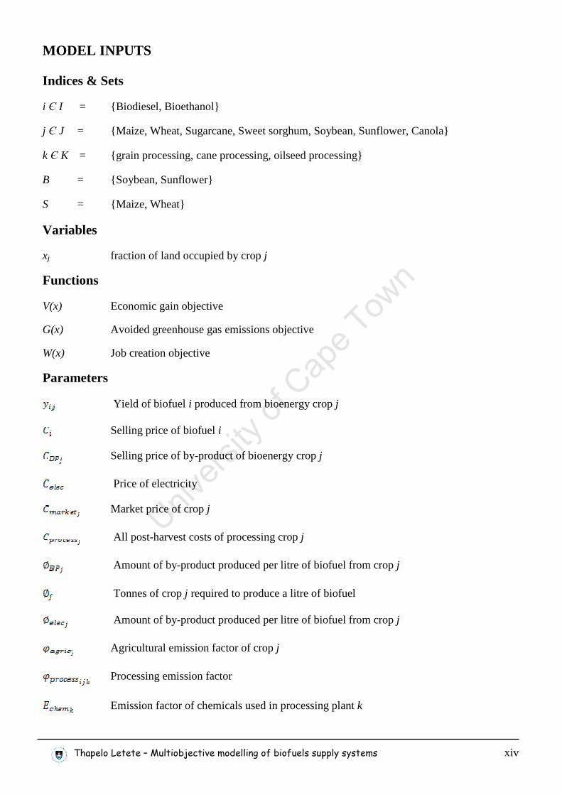
MODEL INPUTS
Indices & Sets
i Є I = {Biodiesel, Bioethanol}
j Є J = {Maize, Wheat, Sugarcane, Sweet sorghum, Soybean, Sunflower, Canola}
k Є K = {grain processing, cane processing, oilseed processing}
B = {Soybean, Sunflower}
S = {Maize, Wheat}
Variables
xj fraction of land occupied by crop j
Functions
V(x) Economic gain objective
G(x) Avoided greenhouse gas emissions objective
W(x) Job creation objective
Parameters
Yield of biofuel i produced from bioenergy crop j
Selling price of biofuel i
Selling price of by-product of bioenergy crop j
Price of electricity
Market price of crop j
All post-harvest costs of processing crop j
Amount of by-product produced per litre of biofuel from crop j
Tonnes of crop j required to produce a litre of biofuel
Amount of by-product produced per litre of biofuel from crop j
Agricultural emission factor of crop j
Processing emission factor
Emission factor of chemicals used in processing plant k
Univers
ity of
Cap
e Tow
n
Thapelo Letete – Multiobjective modelling of biofuels supply systems xv
Emission factor of fossil energy used in plant k
Emission factor associated with transportation of crop j
Emission factor of transporting biofuel i
Emission factor associated with human labour
Emission factor associated with steel
Emission factor associated with concrete
Labour requirements of processing technology k
Steel requirements of processing technology k
Concrete requirements of processing technology k
Matrix that matches the crops to the correct processing technologies
h = 8 number of working hours per day
W jagrp ,_ Number of permanent agricultural workers required per ha of j grown
Sj Length of farming season for crop j
L jagrt ,_ Temporary agricultural labour required for growing crop j
L kpro, Labour requirements of processing technology k
F ji , Flow of biofuel i produced from crop j
σ land Fraction of the underutilized land that is currently being cultivated
P j Profit made by farmers from selling crop j at market price
P j,2 Profit made by farmers from selling crop j at 2nd grade market price
g2 Fraction of emerging farmers’ grains (maize & wheat) currently sold as second grade
δ j Cost of transporting crop j to processing plant
P sorghumsBP _, Profit made by farmers from selling sweet sorghum grain
Univers
ity of
Cap
e Tow
n
Thapelo Letete – Multiobjective modelling of biofuels supply systems xvi
ACRONYMS
CAIT Climate Analysis Indicator Tool
CDF Clean Development Fund
CO2-eqt Carbon dioxide equivalent
DCs Developing countries
DEAT Department of Environment and Tourism
DME Department of Minerals and Energy
DoA Department of Agriculture
DPLG Department of Local and Provincial Government
DSS Decision support system
ERC Energy Research Centre
FDC Free State Development Corporation
GHG Greenhouse gas
IDP Integrated Development Plan
IPCC International Panel on Climate Change
LDCs Least Developed countries
LED Local Economic Development
LIHDs Low-input high-diversity mixtures
LTMS Long Term Mitigation Scenarios
NEB Net Energy balance
NEB-ratio Net Energy Balance ratio
NICs Newly Industrialized Countries
RIDCs Rapidly Industrialising
UNFCCC United Nations Framework Convention on Climate Change
Univers
ity of
Cap
e Tow
n
Thapelo Letete – Multiobjective modelling of biofuels supply systems 1
1. INTRODUCTION
This chapter sets the scene for the thesis by outlining the background of the project, the problem
addressed by the thesis and the key objectives. The scope is laid out and the chapter then concludes by
summarizing the structure of the rest of this thesis.
1.1. Background
Biomass was the world’s primary source of energy in the transportation sector until the late 1920’s,
which saw the emergence of seemingly abundant and cheaper petroleum oil. So the oil liquid fuel
paradigm took root and gave rise to the petroleum refinery and distribution network. Everyone simply
abandoned biomass and focused on petroleum oil. Even machinery which was originally designed to run
on ethanol from biomass was modified to run only on gasoline (Miller, 2005).
The energy crisis of the 1970s, however, sparked renewed interest in the synthesis of fuels and materials
from bio-resources. But this interest quickly waned as the oil price fell again in the decades that
followed and global consumption of liquid petroleum tripled in the ensuing years. With the current
global energy consumption, the demand of oil is projected to grow by more than 50% by 2025, and most
experts agree that we will soon reach “peak oil”, if we have not reached it already (Ragauskas et al.,
2006;Buchanan, 2006). Even with new technologies and new sites to search, oil will run out in 50 to 100
years.
This depletion of crude petroleum oil is not the only problem of reliance on petroleum fuels for energy;
the negative environmental effects associated with their continued use pose even further problems.
According to the International Panel on Climate Change (IPCC, 2007) the use of fossil fuels is the main
reason for the increased atmospheric concentration of carbon dioxide which is resulting in
anthropogenic global climate change. Indeed the warming of the climate system is indisputable, “as is
now evident from observations of increased global average air and ocean temperatures, widespread
melting of snow and ice and rising global average sea level” (IPCC, 2007).
These are some of the reasons which, in recent years, have forced the world to rethink the role of
biomass in the energy sector. Since 1976 there has not been a single new petroleum refinery built in the
United States. Instead more than 85 bioethanol plants, based on the standard sugar fermentation process
using maize kernels as feedstock, have been built (Miller, 2005). The same is true for the world’s largest
bioethanol producer Brazil. It would thus seem that the world is experiencing the beginning of an
entirely new energy paradigm.
Univers
ity of
Cap
e Tow
n
Thapelo Letete – Multiobjective modelling of biofuels supply systems 2
Biomass is a renewable energy resource with the advantage of being greenhouse gas neutral if used
efficiently. If derived from sustainable agricultural practices, biomass energy also provides an
opportunity for developing countries to utilise their own resources, resulting in increased job and wealth
creation, as well as the attraction of international benefits and investment (Ugarte, 2005). With modern
technologies, biomass can be converted into useful energy carriers: heat, electricity and biofuels (solid,
liquid and gaseous fuels). Of these bioenergy carriers, liquid biofuels have, in recent years, received the
most attention throughout the world for their potential to substitute conventional transportation fuels.
According to Hamelinck (2004), the global transportation sector is almost entirely based on fossil fuel
and it represents about 27% of the world’s secondary energy consumption; a percentage that is expected
to increase to 29 – 32 % in 2050. This implies that biofuels are envisaged to take up a significant share
of the world’s energy consumption in the coming years.
South Africa has also recognised the need to reduce its dependence on fossil fuels as the primary source
of energy. In 2003 South Africa’s deputy minister of Minerals and Energy (DME, 2003) declared that
the time has come for renewable energy to take its rightful place in the South African Energy Sector,
and to play a significant role in contributing towards sustainable development. It was in this context that
the government established a target for 2013 of 10,000 GWh renewable energy contributions to the final
national energy consumption, of which 30% should be in the form of liquid biofuels (DME, 2007;DME,
2003).
Contrary to the international situation, however, the main driver for the development of a biofuel
industry in South Africa is neither the constantly increasing oil prices, the issue of energy security nor
anthropogenic climate change, but the need to create a link between the country’s first and second
economies. This involves stimulating economic development and reducing poverty by creating
sustainable income-earning opportunities in under-developed areas (DME, 2007). According to the
Industrial Biofuels Strategy of the Republic of South Africa (DME, 2007), the focus is primarily on “the
promotion of farming in areas that were previously neglected by the apartheid system and areas of the
country that did not have market access for their produce, most of these areas are in the former
homeland areas”. Thus the issue of land use is central to the development of South Africa’s biofuel
industry.
While the National Biofuels Study, which was commissioned to support the development of the Biofuels
Strategy, shows that an agriculture-based biofuel industry in South Africa is likely to encounter
problems relating to small-scale subsistence farming, emerging farmers and scarcity of arable land, it
gives no insight into how efficient land use may be achieved (National Biofuels Task Team, 2006).
Moreover, the National Biofuels Study is primarily an economic impact study, and therefore its analyses
were mainly concerned with optimization of economic benefits, and only when this had been achieved
Univers
ity of
Cap
e Tow
n
Thapelo Letete – Multiobjective modelling of biofuels supply systems 3
were the analyses of maximizing the social and environmental benefits conducted. Thus the overall
interdependence of the different socio-economic and environmental objectives of the National Biofuels
Strategy and the subsequent effect that their optimization has on land use are still largely unknown.
1.2. Problem Statement
Globally the increasing shift from the use of conventional petroleum fuels in the transportation sector to
liquid biofuels is mainly motivated by issues of energy security and anthropogenic global warming. In
South Africa, however, the development of a biofuel industry is primarily seen as a local economic
development and poverty alleviation issue, especially in those areas of the country that were previously
neglected by the apartheid regime. The Biofuels Industrial Strategy of South Africa is thus structured
such that it centres on the development of agriculture in these areas. In fact, only those biofuels
produced from crops grown in these areas will qualify for government support. Arable land, however, is
very limited in South Africa; with only 14% of the total land in South Africa receiving enough rainfall
for arable crop production. Clearly the percentage of arable land that fits the criteria of the Industrial
Biofuels Strategy and that can be dedicated to biofuel production is even smaller. There is, therefore, a
need to facilitate the effective utilisation of this limited resource if sustainability and maximum return on
input are to be achieved.
Given a fixed amount of arable land dedicated to biofuels production, a choice of energy crops that can
be locally grown and a choice of processing technologies for these crops, the problem is that of land-use
optimization, such that the economic, social and environmental objectives of the National Biofuels
Strategy are satisfied in the best possible way.
1.3. Objectives
Specific objectives of this thesis are:
1. To analyse the Life-cycle energy balances, climate change mitigation potentials and economic
performances of the various biofuel supply chains available to South Africa, involving the
different bioenergy crops that can be grown locally
2. To determine the environmental effects of land use change in the development of an agriculture-
based biofuels industry in South Africa
3. To develop a multiobjective model for minimizing land use in the biofuel industry, while
optimizing one objective from each of the economic, social and environmental spheres of the
industry
4. To demonstrate the use of multiobjective optimisation models as decision support systems for
bioenergy decisions both at national and local government levels
Univers
ity of
Cap
e Tow
n
Thapelo Letete – Multiobjective modelling of biofuels supply systems 4
1.4. Key Questions
The thesis seeks to answer the following key questions:
• Based on the current agricultural practices and various crop yields in the country, how much
return on energy input can be achieved by the different biofuel supply chains?
• What are the climate change implications of land use change in the development of a biofuel
industry in South Africa? If there are negative effects, how long would it take for the biofuels to
ultimately repay the initial “carbon debt”?
• Given a fixed amount of arable land and a choice of energy crops that can be locally grown,
which crop distribution will result in optimum land use in the South African biofuel industry?
What are the factors affecting this optimum crop distribution?
• What are the land use options available to South Africa to achieve its biofuel target of 2% market
penetration of liquid road transport fuels involving B2 (2% biodiesel mix with 98% diesel) and
E8 (8% bioethanol blend with 92% petrol) beyond 2013 with minimal resource utilization?
• What effects do commodity and fossil fuel prices have on the optimum crop distributions?
1.5. Scope and Limitations
This study analyses the possible biofuel supply chains for an agriculture-based biofuels industry in
South Africa. This includes agricultural land and practices, technologies, fuel prices and commodity
prices specific to South Africa. The overall optimisation model algorithm, however, is developed as an
open multi-objective optimisation model that can easily be applied to other areas, provided that
appropriate physical data and constraints for that area are available.
The main limitation of this thesis is that the life-cycle analyses carried out herein are only cradle-to-
blending-station assessments which exclude the end-use of the biofuels, thus the results obtained cannot
readily be compared with results of the studies assessing the energy balances and environmental burdens
of the different crops on the basis of passenger kilometres driven. Another limitation to the analyses in
this study is that ability of the livestock industry to absorb the oilmeal by-products from biodiesel
processing has not been considered.
Univers
ity of
Cap
e Tow
n
Thapelo Letete – Multiobjective modelling of biofuels supply systems 5
1.6. Thesis Outline
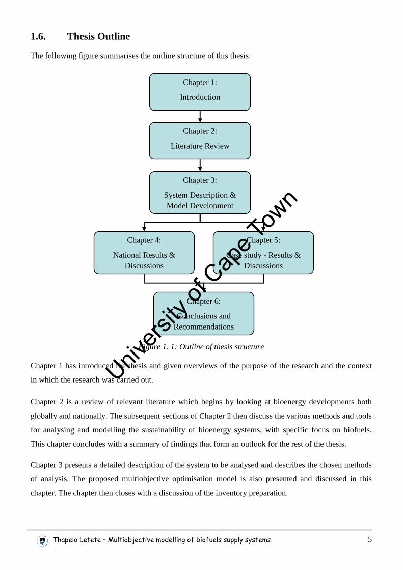
The following figure summarises the outline structure of this thesis:
Figure 1. 1: Outline of thesis structure
Chapter 1 has introduced the thesis and given overviews of the purpose of the research and the context
in which the research was carried out.
Chapter 2 is a review of relevant literature which begins by looking at bioenergy developments both
globally and nationally. The subsequent sections of Chapter 2 then discuss the various methods and tools
for analysing and modelling the sustainability of bioenergy systems, with specific focus on biofuels.
This chapter concludes with a summary of findings that form an outlook for the rest of the thesis.
Chapter 3 presents a detailed description of the system to be analysed and describes the chosen methods
of analysis. The proposed multiobjective optimisation model is also presented and discussed in this
chapter. The chapter then closes with a discussion of the inventory preparation.
Chapter 1:
Introduction
Chapter 3:
System Description & Model Development
Chapter 2:
Literature Review
Chapter 4:
National Results & Discussions
Chapter 5:
Case study - Results & Discussions
Chapter 6:
Conclusions and Recommendations
Univers
ity of
Cap
e Tow
n
Thapelo Letete – Multiobjective modelling of biofuels supply systems 6
Chapter 4 and Chapter 5 are essentially results and discussion chapters. While the former presents and
discusses results on a national scale, the latter is a case study that applies the developed model to support
decision-making at local municipal level.
In Chapter 6 the findings of the preceding two chapters are used to draw conclusions in line with the key
questions, after which relevant recommendations are then made.
Univers
ity of
Cap
e Tow
n
Thapelo Letete – Multiobjective modelling of biofuels supply systems 7
2. LITERATURE REVIEW
In this chapter, the potential contribution of bioenergy to future global energy supply is discussed,
followed by the bioenergy situation in South Africa. Energy planning by mathematical modelling is also
reviewed with focus on the appropriate model for South Africa.
2.1. Review of Bioenergy
2.1.1. Bioenergy Supply Chains
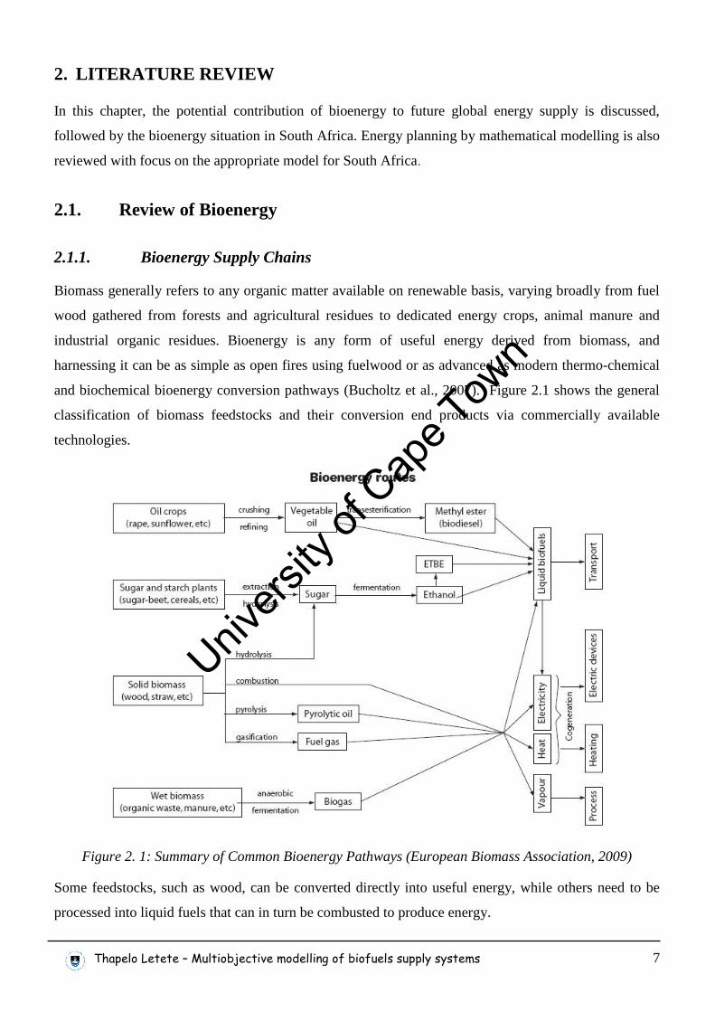
Biomass generally refers to any organic matter available on renewable basis, varying broadly from fuel
wood gathered from forests and agricultural residues to dedicated energy crops, animal manure and
industrial organic residues. Bioenergy is any form of useful energy derived from biomass, and
harnessing it can be as simple as open fires using fuelwood or as advanced as modern thermo-chemical
and biochemical bioenergy conversion pathways (Bucholtz et al., 2007). Figure 2.1 shows the general
classification of biomass feedstocks and their conversion end products via commercially available
technologies.
Figure 2. 1: Summary of Common Bioenergy Pathways (European Biomass Association, 2009)
Some feedstocks, such as wood, can be converted directly into useful energy, while others need to be
processed into liquid fuels that can in turn be combusted to produce energy.
Univers
ity of
Cap
e Tow
n
Thapelo Letete – Multiobjective modelling of biofuels supply systems 8
2.1.2. The Potential of Biomass contribution to Energy
Global fossil fuel use in 1994 was estimated at 302 EJ, while biomass, mostly used for cooking over
open fires and mostly unreported in global statistics, was estimated at 55EJ (Hall et al., 1993). In 2004
the total global energy consumption was reported to be 470 EJ and is expected to reach 700 EJ (EIA,
2006) and 1041 EJ (World Energy Council, 2007) in 2025 and 2050 respectively.
Many studies have been undertaken to assess the potential contribution of biomass to the global energy
network. In an analysis of a selection of seventeen studies on the potential contribution of bioenergy to
the global energy supply, Berndes et al (2003) found the conclusions to vary from below 100 EJ/yr to
above 400 EJ/yr in 2050. The Group Planning Division of the Shell International Petroleum Company
developed a predictive energy scenario which showed a dramatic expanding role for biomass beginning
early in the 21st century, rising to over 200 EJ/yr by 2050 (Kassler, 1994). The Second Assessment
Report of the Intergovernmental Panel on Climate Change (IPCC) also shows a biomass-intensive
energy scenario for the world that predicts 75 EJ of modernized, commercial bioenergy production in
2025, reaching over 180 EJ of sustainable biomass use by 2050 (Williams, 1995).
In a preliminary analysis, Marrison and Larson (1996) reported a biomass potential to produce
bioenergy of 18.4 EJ/yr in 2025 for Africa alone, while Smeets et al. (2007) estimate it to be between 48
EJ/yr and 389 EJ/yr in 2050, with Sub-Saharan Africa accounting for more than 90%.
2.1.3. Biofuels
Of all modern bioenergy carriers, liquid biofuels have, in recent years, received the most attention
throughout the world as potential substitutes of conventional transportation fuels. A biofuel is broadly
defined as a solid, liquid, or gas fuel derived predominantly or exclusively from biomass. Liquid
biofuels have recently been classified as “first-generation” or “second-generation” biofuels depending
on the type of feedstock or technology used to manufacture them. According to the United Nations
Conference on Trade and Development (2008), there are no strict technical definitions for these two
terms.
First-generation biofuels are primarily produced from sugars, starches, oil bearing crops or animal fats,
and tend to only utilize those portions of the plant biomass that are also used as food. Technologies for
producing these fuels are generally well established and significant commercial quantities of first-
generation biofuels are already produced in many countries around the world.
Second-generation biofuels are those produced from non-edible lignocellulosic biomass such as residues
from food crop production or forestry biomass. Technologies for these fuels are neither as well
Univers
ity of
Cap
e Tow
n
Thapelo Letete – Multiobjective modelling of biofuels supply systems 9
established nor as mature as those of first-generation biofuels, hence the former are not yet produced
commercially in any country (UNCTAD, 2008).
The two most common first-generation biofuels are bioethanol and biodiesel:
2.1.3.1. Bioethanol
The most widely-used first-generation liquid biofuel is ethanol (or ethyl alcohol) produced by the
biological fermentation of plant sugars and starches. While sugarcane and maize are the most common
feedstocks for ethanol production, other feedstocks include wheat, cassava, potatoes, sugar beets and
most recently sweet sorghum. Bioethanol can either be blended with petrol to increase the octane level
of petrol and used in existing spark ignition engines, or used unblended, in modified 100% alcohol-
fuelled engines or even used as hydrous ethanol in any proportion with petrol in flexi-fuel vehicles. The
latter practice is common in Brazil (Macedo et al., 2008).
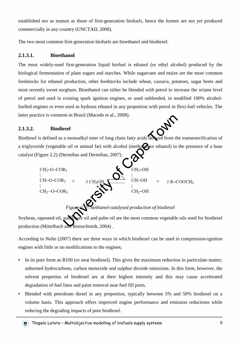
2.1.3.2. Biodiesel
Biodiesel is defined as a monoalkyl ester of long chain fatty acids derived from the transesterification of
a triglyceride (vegetable oil or animal fat) with alcohol (methanol or ethanol) in the presence of a base
catalyst (Figure 2.2) (Dermibas and Dermibas, 2007).
Figure 2. 2: methanol-catalysed production of biodiesel
Soybean, rapeseed oil, sunflower oil and palm oil are the most common vegetable oils used for biodiesel
production (Mittelbach and Remschmidt, 2004) .
According to Nolte (2007) there are three ways in which biodiesel can be used in compression-ignition
engines with little or no modifications to the engines;
• In its pure form as B100 (or neat biodiesel). This gives the maximum reduction in particulate matter,
unburned hydrocarbons, carbon monoxide and sulphur dioxide emissions. In this form, however, the
solvent properties of biodiesel are at their highest intensity and this may cause accelerated
degradation of fuel lines and paint removal near fuel fill ports.
• Blended with petroleum diesel in any proportion, typically between 5% and 50% biodiesel on a
volume basis. This approach offers improved engine performance and emission reductions while
reducing the degrading impacts of pure biodiesel.
Univers
ity of
Cap
e Tow
n
Thapelo Letete – Multiobjective modelling of biofuels supply systems 10
• As an additive to petroleum diesel, typically in proportions of 1%-2% biodiesel on volume basis, to
enhance the lubricity of petroleum diesel.
2.2. Bioenergy developments in South Africa
South Africa’s economy is one of the most energy-intensive in Africa, heavily relying on fossil fuels as
a primary source of energy. The national energy supply is dominated by coal, which accounts for more
than 70% of the country’s fossil-based energy supply, while biomass is estimated to supply just below
20% of the national energy consumption, mostly in the form of fuel wood consumed in relatively low-
efficiency devices or waste products used for electricity and process heat generation in the sugar, pulp
and paper industries (Davidson, 2006).
As a result of this high dependence on coal, South Africa is by far the most carbon emission-intensive
country in the continent and one of the largest greenhouse gas emitters in the world (Figure 2.3). In
terms of energy CO2 emissions per GDP per purchasing power parity (GDP-ppp), South Africa ranks 24
in the world, surpassing world giants like the USA and Brazil as shown in Figure 2.4. According to data
from the Climate Analysis Indicator Tool (CAIT) (2005), South Africa can be ranked between 14 and
65, out of over 200 countries in the world, in terms of greenhouse gas emissions, depending on the
number of gases and emission sources being considered. In light of the increasing evidence of global
climate change due to increased concentrations of greenhouse gases in the atmosphere, these emission
rankings of South Africa have been points of much discussion in recent years, both locally and in the
context of international efforts against climate change to which South Africa is party.
The most relevant international climate change effort is the Kyoto Protocol – a multilateral agreement of
the United Nations Framework Convention on Climate Change (UNFCCC) to which South Africa
acceded in March 2002. This protocol is aimed at achieving stabilization of greenhouse gas emissions in
the atmosphere at a level that would prevent dangerous anthropogenic interference with the climate
system. Under both the convention and the protocol, however, South Africa is recognised as a
developing country and as a result, it is not committed to any emission reduction targets during the first
commitment period of the protocol ending in 2012.
Univers
ity of
Cap
e Tow
n
Thapelo Letete – Multiobjective modelling of biofuels supply systems 11
0
5
10
15
20
25
30
35
40
45
USA Annex_1 Brazil SouthAfrica
EuropeanUnion (29)
World non-Annex_1
Sub-Saharan
Africa
China India
Country/Region
1000
Mt C
O2e
qt p
er y
ear
/ Ton
CO
2 pe
r ca
pita
Ton CO2/capita
1000 Mt CO2 eqt/yr
Figure 2. 3: Comparison of country and regional annual emissions, 2000. [Letete and Guma (2008)
using data from Climate Analysis Indicator Tool(2005)]
0
200
400
600
800
1,000
1,200
1,400
1,600
Russia SouthAfrica
China USA non-Annex1
World Annex 1 India Brazil Sub-Saharan
Africa
Country/Region
Em
issi
ons
per
GD
Ppp
p [to
n C
O2/
Mill
ion
2000
US
$]
Figure 2. 4: Comparison of country and regional CO2 emissions per GDP-ppp (2000 US$) from energy and cement production, 2002 [Letete and Guma (2008) using data from Climate Analysis Indicator Tool
(2005)]
Univers
ity of
Cap
e Tow
n
Thapelo Letete – Multiobjective modelling of biofuels supply systems 12
As the end of the first commitment period of the protocol approaches, however, the UNFCCC has called
for stakeholders and governments to come up with options for advancing the international climate
change efforts beyond 2012, and below is a summary of the most favoured approaches being proposed
(Hohne and Moltmann, 2007;Bodansky, 2004):
1. Contraction and convergence: Under this regime all countries participate with quantified
emission targets. Firstly, all countries agree on a path of future global emissions leading to a
targeted long-term stabilization of greenhouse concentrations, and then targets are set for
individual countries such that per capita emissions converge to the same level for all countries by
an agreed time.
2. Common but differentiated convergence: This approach requires the per capita emissions of
Annex I countries to immediately start converging to a stabilization level equal for all countries
within a set period, while for individual non-Annex 1 countries convergence only starts when
their per capita emissions reach a certain percentage threshold of the global average.
3. Multistage: In this approach countries participate in several stages, with differentiated
commitments, and countries graduating to higher stages when they exceed certain thresholds. In
the first stage countries have no commitments at all, while in the last stage countries receive
absolute emission reduction targets until all countries stabilize their per capita emissions to a
specified level below 1990 levels.
4. Global Triptych: This is a method of allocating emission allowances among all countries based
on several national indicators, while taking into account emission reduction potentials for the
different countries. The method calculates emission allowances for the various sectors which are
then added to obtain a binding national target.
5. Brazilian Proposal: This approach proposes burden-sharing of greenhouse gas reduction based
on the countries’ historical responsibility for existing temperature change. As initially presented,
this proposal called for reduction commitments of developed countries or contribution to a Clean
Development Fund (CDF) if they fail to meet these commitments. The CDF would be used to
fund clean development projects and adaptation projects in developing countries.
6. South-North Dialogue: This approach separates countries into six groups, each with a different
mitigation, adaptation and financial set of commitments. Under this approach, Annex II countries
take on more strict commitments than Kyoto commitments, while other Annex I countries
continue to have targets similar to those required by the Kyoto protocol. Newly Industrialized
Countries (NICs) and Rapidly Industrialising Developing Countries (RIDCs) would also have
Univers
ity of
Cap
e Tow
n
Thapelo Letete – Multiobjective modelling of biofuels supply systems 13
quantified targets, but only on condition that all major Annex I have binding quantified emission
reduction obligations. For RIDCs the targets would only be binding on receipt of significant
financial and technological assistance from Annex II countries. Instead of targets, Other
Developing countries (DCs) and Least Developed countries (LDCs) would adopt obligatory and
optional Sustainable Development Policies respectively.
From these proposals, it is clear that most of the international community supports some level of
commitment of some of the developing countries in the protocol. This means that South Africa’s role in
the protocol is very likely to change in the second commitment period to be agreed upon at the 15th
United Nations Climate Change Conference of Parties in Copenhagen in 2009. Any commitment for
South Africa in the protocol would thus require the country to seriously consider the role of renewable
energy sources, including biomass, in the country’s economy.
Regardless of the outcome of the Copenhagen negotiations, however, the South African government has
already committed to ensuring a climate resilient and low-carbon economy and society, and
consequently outlined its vision, strategic direction and policy framework on climate change in July
2008 (Schalkwyk, 2008). Informed by the Long Term Mitigation Scenarios (LTMS) process, the
government’s strategy includes setting mandatory targets for electricity generated from both renewable
and nuclear energy sources and using feed-in-tarrifs as incentives for renewable energy. The final
national policy on climate change is envisaged to be adopted by the end of 2010.
Independent of the climate change threat, still, the South African minister of Environmental Affairs and
Tourism, Martinus van Schkalwyk, has also declared that another challenge for South Africa in the
coming decades “will be to diversify our energy dependence – developing alternative renewable and
non-carbon based sources of energy (DEAT, 2005).” Echoed also in the government’s climate change
policy framework, the need for diversifying the country’s energy mix and promoting alternative
transport fuels has been acknowledged in South Africa as early as the late 1990’s, and since then, the
government has developed various policies and frameworks aimed at achieving this goal. In 2003, the
government published a White Paper on Renewable Energy (DME, 2003); a policy document aimed at
creating conditions to bring about integration of renewable energies into the country’s mainstream
energy economy. The economic, social, and environmental benefits offered by renewable energy are
identified in this document as follows:
• Renewable sources of energy have substantial potential to increase security of supply by
diversifying the energy supply portfolio and thereby contributing towards a long-term sustainable
energy future.
Univers
ity of
Cap
e Tow
n
Thapelo Letete – Multiobjective modelling of biofuels supply systems 14
• Renewable energy generation results in the emission of less greenhouse gases, airborne
particulates and other pollutants when compared to fossil fuels.
• Renewable energy can be generated centrally and distributed for use near its point of production
thus reducing the cost of infrastructure required for energy distribution and energy delivery
losses.
• A renewable energy industry that meets international standards will attract investment that would
otherwise be lost to the country.
• A sustainable renewable energy programme has the potential for increased industrial growth and
thereby supporting a variety of national priorities, including job-creation and sustainable
development.
• Renewable energy technologies provide significant potential export market opportunities to the
southern African region.
In view of these benefits, the White Paper clearly sets out the government’s long term goal as the
establishment of a South African renewable energy industry that produces modern energy carriers and
offering in future years a sustainable, fully non-subsidised alternative to fossil fuels. As a first step
towards achieving this goal, the government has set a target of “10,000 GWh (0.8 Mtoe) renewable
energy contribution to final energy consumption by 2013, to be produced mainly from biomass, wind,
solar and small-scale hydro,” and for utilization in power generation and other technologies like solar
water heating and biofuels (DME, 2003).
In 2007, the government released a Biofuels Industrial Strategy of the Republic of South Africa (2007)
targeted at “creating jobs in the energy-crop and biofuel chain, and to act as a bridge between the first
and second economies.” This strategy stresses on the promotion of “currently underutilized, high
potential agricultural areas” that were previously neglected by the apartheid system and areas that had
no market to their produce, most of which are located in the former homelands. The strategy proposes a
5 year pilot period in which a biofuels average market penetration of 2% of liquid road transport fuels
(petrol and diesel) will be targeted. This target amounts to 30% of the national Renewable Energy target
for 2013, and to meet it, a scenario of E8 (national basis of 8% bioethanol and 92% fossil petrol) and B2
(national basis of 2% biodiesel and 98% fossil diesel) will be adopted (DME, 2007). The strategy,
however, has some ambiguities because it does not show how this E8 and B2 scenario is supposed to
achieve a 2% national market penetration of biofuels. For food security purposes, however, the strategy
proposes that maize be excluded as a feedstock for bioethanol production in this pilot period of the
strategy.
There are currently no large scale biofuel producers in South Africa, but there is a lot of interest both in
the agricultural and corporate world. Sugar producers and maize farmers represent the majority of the
Univers
ity of
Cap
e Tow
n
Thapelo Letete – Multiobjective modelling of biofuels supply systems 15
parties looking to drive the South African bioethanol industry, with some of the former having been
involved in bioethanol production for the potable and export alcohol markets even before the National
Biofuels Industry Strategy was released (DME, 2007). The maize-to-ethanol industry, however, has
never taken off due to the restrictions of the National Biofuels Strategy.
Biodiesel, mostly from recycled sunflower oil, is produced on small-scale (less than 300,000 litres per
year) by many farmers and small companies across the country (Murray, 2008). Virgin Soybean,
sunflower and canola oils have also been used for biodiesel production.
2.3. Sustainability of bioenergy from a life-cycle perspective
Life-cycle analysis is an approach for systematically evaluating the environmental effects of a product or
service from the initial gathering of raw materials from the earth until the point at which all residuals are
returned to the earth. This concept, known as “cradle to grave”, provides a holistic environmental
analysis by considering the potential impacts at every stage of the life a product, process, package or
activity (Vigon et al., 1993).
Although it is not a single uniform method, life-cycle assessment as a tool for measuring environmental
impacts has been standardized to allow comparisons. According to the International Organization for
Standardization (ISO, 1997), there are four separate yet interrelated components to every life-cycle
assessment:
1 Goal definition and scoping: This entails clearly defining the goal of the study, the functional
unit with which alternative products or services are to be compared, the unit processes making
up the systems under study and the boundaries of the system. This is the step that defines the
analysis and determines the type and detail of information required in the subsequent sections.
2 Inventory Analysis: This is a technical, data-based stage where identification and quantification
of energy use, raw material requirements, environmental emissions and waste given off for the
entire life-cycle of the product or activity under study are made.
3 Impact Analysis: This is a quantitative evaluation of the impacts of resource requirements and
environmental burdens identified in the inventory analysis stage. The eight most commonly
used impact categories are listed below:
• Natural resource depletion
• Global warming potential
• Ozone depletion potential
• Ecological toxicity potential
Univers
ity of
Cap
e Tow
n
Thapelo Letete – Multiobjective modelling of biofuels supply systems 16
• Acidification potential
• Human toxicity
• Photochemical oxidant creation potential
• Eutrophication potential
These impacts are quantified by internationally-agreed units and potency factors for each source
category.
4 Interpretation: At this stage impacts are assessed, and a systematic evaluation of the needs and
opportunities to reduce the environmental burdens is employed. This analysis may be both
quantitative and qualitative in nature, and many different approaches have been used depending
on the goal of the life-cycle assessment.
In bioenergy systems, life-cycle assessment is commonly used to describe environmental sustainability
and to “determine whether bio-based fuels (biofuels) are helping us to achieve the goal of providing
environmentally sustainable transportation” (von Blottnitz and Curran, 2007).
Apart from the “standardized” life-cycle assessment, two other tools have been widely used to determine
the sustainability of bioenergy systems; energy balancing and carbon balancing. Although these methods
all stem from a common life-cycle approach, these latter two methods are usually simpler and more
specific in nature as described below:
2.3.1. Energy balancing
In an energy balance analysis all the fossil energy inputs in upstream processing of the biofuel are
calculated and compared with the energy value of the biofuel product and its by-products.
Two indicators are usually employed in energy balance analyses; the first is the Net Energy balance
(NEB) defined as:
and second is the Net Energy Balance ratio (NEB-ratio) defined as:
where Energy-InputTotal is the total fossil energy input in upstream processing of the biofuel and Energy-
OutputTotal is the energy retrieved from the biofuel and its by-products.
Univers
ity of
Cap
e Tow
n
Thapelo Letete – Multiobjective modelling of biofuels supply systems 17
For a bioenergy system to be considered to have some renewability, it must have a positive NEB or
NEB-ratio greater than 1, the higher the ratio, the closer the system approaches to complete renewability
(complete renewability is a theoretical term that defines a system with a ratio of infinity) (von Blottnitz
and Curran, 2007).
2.3.2. Carbon balancing
Carbon balancing evaluates the net greenhouse gas emissions of the biofuel through its life-cycle. The
most common indicator employed in carbon balancing is Avoided emissions which is defined as: The
difference of the greenhouse gas emissions that would have resulted from the production, transportation
and use of the products that are replaced by all biomass products (GHG-emissionsReplaced-products) and the
greenhouse gas emissions released in the upstream production of the biofuel (GHG-emissionsBiofuel-
production) as shown below:
Both GHG-emissionsReplaced-products and GHG-emissionsBiofuel-production are usually expressed in units of kg
CO2-equivalent.
2.4. Concerns over biofuels
In 2003, Berndes et al. (2003) showed that all the studies undertaken on future bioenergy potential do
not provide much insight on how the expanding bioenergy sector will interact with other land uses, and
the socio-economic consequences of realizing the reported bioenergy potentials. In particular, the
development of the food and materials sector is exogenously defined in these studies, and the bioenergy
sector evolves in parallel, using residues and land not required for food or materials production. Hence,
according to these studies, the expanding bioenergy sector does not, by definition, affect the food and
materials sector. Recent studies (Searchinger et al., 2008;Fargoine et al., 2008), however, have shown
that bioenergy industries, especially biofuels, not only compete with other commodities for land but may
actually drive all other land-use competitors away in the long run.
The following consequences have been observed to arise from this competition of biofuels with other
commodities over land:
1. Accelerated global warming: As a result of increasing demand for biofuels, previously
undisturbed ecosystems, especially in the Americas and Southeast Asia are being cleared out to
make way for biofuel crops; In Malaysia and Indonesia, tropical rain forests are being burned
and converted to palm oil plantations for biodiesel production, while grassland in the United
States, primarily rangeland or former cropland currently retired in conservation programs, is
Univers
ity of
Cap
e Tow
n
Thapelo Letete – Multiobjective modelling of biofuels supply systems 18
being converted to maize production. Perhaps the case that has brought the most attention is that
of the Brazilian Amazon and Cerrado, which are rapidly being converted to sugarcane and
soybean plantations.
According to Fargione et al. (2008) soils and plant biomass are the two largest biologically
active stores of terrestrial carbon, together storing up to 2.7 times more carbon than the
atmosphere, and converting these native habitats to cropland not only takes away the dearly
needed sinks of CO2, but releases all this stored CO2 into the atmosphere, leading to accelerated
anthropogenic climate change.
2. Food price inflation: Studies have also shown that the rise in tortilla prices in Mexico and flour
prices in Pakistan can be associated with the increasing demand for food-based biofuels in the
Americas and Southeast Asia (Grunwald, 2008). As more grains and oilseed crops are diverted
from the food market to the biofuel market, a shortage in food availability is observed, leading
to food price increases. According to Searchinger et al. (2008) and Grunwald (2008) this
increase in food prices is another cause for deforestation in the Brazilian Amazon and Cerrado;
as ethanol demand for maize in the United States increases, soybean and wheat farmers switch
to maize, causing the prices of maize, soybeans and wheat to increase by 40%, 20% and 17%
respectively. In response to these price increases Brazilian farmers further expand into fields
previously used as cattle pastures, displacing ranchers, who in turn clear grazing lands in the
Cerrado and the Amazon.
The global warming potentials of the prolonged CO2 emissions as a result of burning or microbial
decomposition of organic carbon stored in plants and soils when native habitats are converted to biofuel
croplands have been intensively studied by Fargione et al. (2008). Looking only at the amount of CO2
released in the first 50 years of this process, which they refer to as the “carbon debt”, Fargione et al.
have shown that the debt can be repaid by biofuels over time, provided that the production and
combustion of the biofuels have net greenhouse gas emissions that are less than the life cycle emissions
of the fossil fuels they displace.
Fargione et al. went further to calculate the biofuel carbon debts and the number of years required to
repay these debts for the Brazillian, United States, Indonesian and Malaysian native habitat conversions,
and compared them with the cultivation of Low-input high-diversity mixtures (LIHDs) of native
American grassland perennials in retired United States cropland. The results, presented as Figure 2.5
below, showed that biofuels produced from crops grown on degraded cropland, especially perennial
grasses, and waste biomass would minimize habitat destruction, competition with food production and
carbon debts associated with clearing land for biofuel production.
Univers
ity of
Cap
e Tow
n
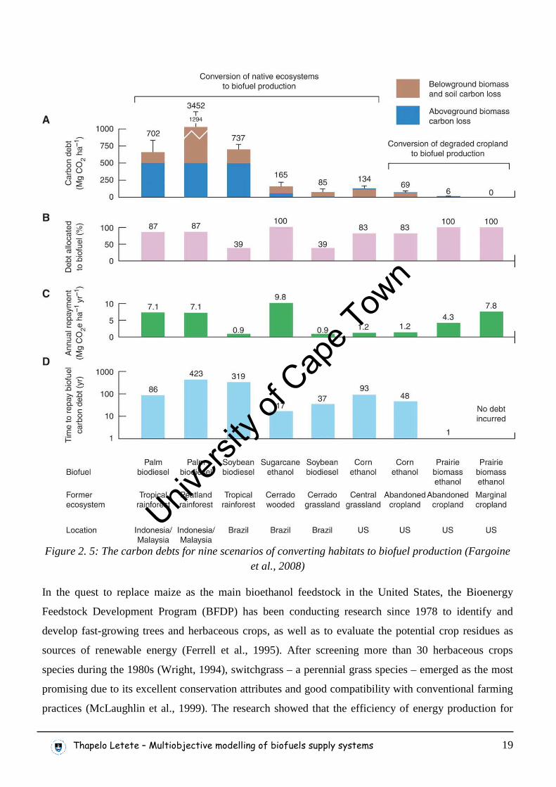
Thapelo Letete – Multiobjective modelling of biofuels supply systems 19
Figure 2. 5: The carbon debts for nine scenarios of converting habitats to biofuel production (Fargoine
et al., 2008)
In the quest to replace maize as the main bioethanol feedstock in the United States, the Bioenergy
Feedstock Development Program (BFDP) has been conducting research since 1978 to identify and
develop fast-growing trees and herbaceous crops, as well as to evaluate the potential crop residues as
sources of renewable energy (Ferrell et al., 1995). After screening more than 30 herbaceous crops
species during the 1980s (Wright, 1994), switchgrass – a perennial grass species – emerged as the most
promising due to its excellent conservation attributes and good compatibility with conventional farming
practices (McLaughlin et al., 1999). The research showed that the efficiency of energy production for
Univers
ity of
Cap
e Tow
n
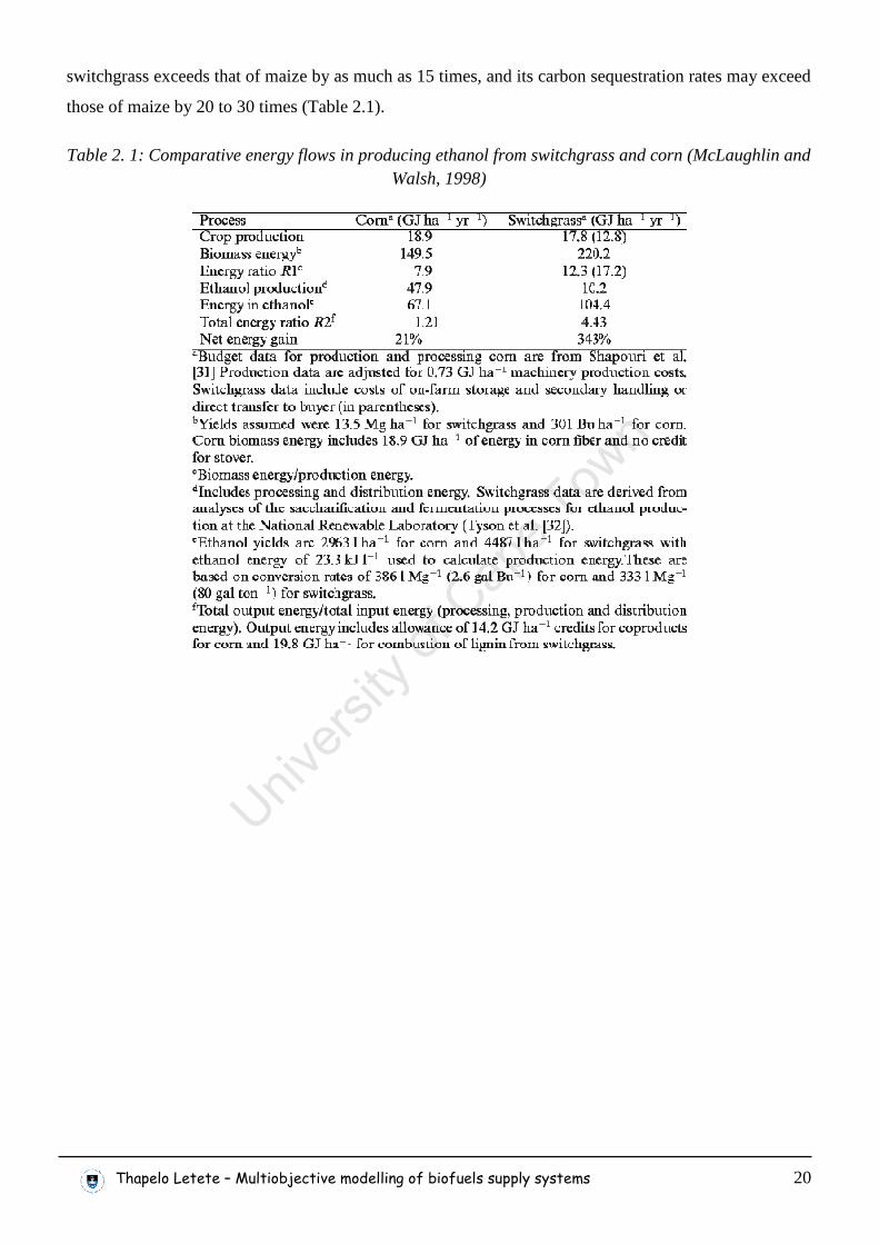
Thapelo Letete – Multiobjective modelling of biofuels supply systems 20
switchgrass exceeds that of maize by as much as 15 times, and its carbon sequestration rates may exceed
those of maize by 20 to 30 times (Table 2.1).
Table 2. 1: Comparative energy flows in producing ethanol from switchgrass and corn (McLaughlin and Walsh, 1998)
Univers
ity of
Cap
e Tow
n
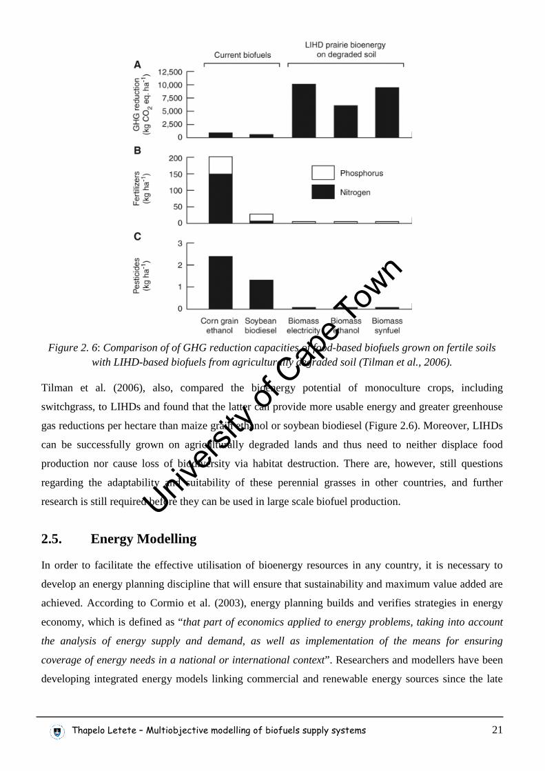
Thapelo Letete – Multiobjective modelling of biofuels supply systems 21
Figure 2. 6: Comparison of of GHG reduction capacities of food-based biofuels grown on fertile soils with LIHD-based biofuels from agriculturally degraded soil (Tilman et al., 2006).
Tilman et al. (2006), also, compared the bioenergy potential of monoculture crops, including
switchgrass, to LIHDs and found that the latter can provide more usable energy and greater greenhouse
gas reductions per hectare than maize grain ethanol or soybean biodiesel (Figure 2.6). Moreover, LIHDs
can be successfully grown on agriculturally degraded lands and thus need to neither displace food
production nor cause loss of biodiversity via habitat destruction. There are, however, still questions
regarding the adaptability and suitability of these perennial grasses in other countries, and further
research is still required before they can be used in large scale biofuel production.
2.5. Energy Modelling
In order to facilitate the effective utilisation of bioenergy resources in any country, it is necessary to
develop an energy planning discipline that will ensure that sustainability and maximum value added are
achieved. According to Cormio et al. (2003), energy planning builds and verifies strategies in energy
economy, which is defined as “that part of economics applied to energy problems, taking into account
the analysis of energy supply and demand, as well as implementation of the means for ensuring
coverage of energy needs in a national or international context”. Researchers and modellers have been
developing integrated energy models linking commercial and renewable energy sources since the late
Univers
ity of
Cap
e Tow
n
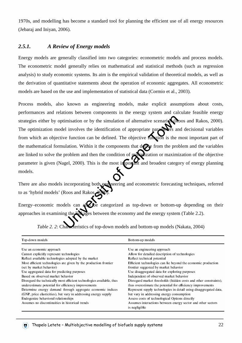
Thapelo Letete – Multiobjective modelling of biofuels supply systems 22
1970s, and modelling has become a standard tool for planning the efficient use of all energy resources
(Jebaraj and Iniyan, 2006).
2.5.1. A Review of Energy models
Energy models are generally classified into two categories: econometric models and process models.
The econometric model generally relies on mathematical and statistical methods (such as regression
analysis) to study economic systems. Its aim is the empirical validation of theoretical models, as well as
the derivation of quantitative statements about the operation of economic aggregates. All econometric
models are based on the use and implementation of statistical data (Cormio et al., 2003).
Process models, also known as engineering models, make explicit assumptions about costs,
performances and relations between components in the energy system and calculate feasible energy
strategies either by optimisation or by the simulation of alternative scenarios (Roos and Rakos, 2000).
The optimization model involves the identification of appropriate parameters and decisional variables
from which an objective function can be defined. The objective function is the most important part of
the mathematical formulation. Within it the components that derive from the problem and the variables
are linked to solve the problem and then the condition of minimization or maximization of the objective
parameter is given (Nagel, 2000). This is the most important and broadest category of energy planning
models.
There are also models incorporating both engineering and econometric forecasting techniques, referred
to as ‘hybrid models’ (Roos and Rakos, 2000).
Energy–economic models can also be categorized as top-down or bottom-up depending on their
approaches in examining the linkages between the economy and the energy system (Table 2.2).
Table 2. 2: Characteristics of top-down models and bottom-up models (Nakata, 2004)
Univers
ity of
Cap
e Tow
n
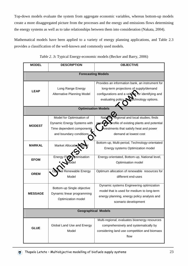
Thapelo Letete – Multiobjective modelling of biofuels supply systems 23
Top-down models evaluate the system from aggregate economic variables, whereas bottom-up models
create a more disaggregated picture from the processes and the energy and emissions flows determining
the energy systems as well as to take relationships between them into consideration (Nakata, 2004).
Mathematical models have been applied to a variety of energy planning applications, and Table 2.3
provides a classification of the well-known and commonly used models.
Table 2. 3: Typical Energy-economic models (Becker and Barry, 2006)
MODEL DESCRIPTION OBJECTIVE
Forecasting Models
LEAP Long Range Energy
Alternative Planning Model
Provides an information bank, an instrument for
long-term projections of supply/demand
configurations and a vehicle for identifying and
evaluating policy and technology options.
Optimisation Models
MODEST
Model for Optimisation of
Dynamic Energy Systems with
Time dependent components
and boundary conditions
National, regional and local studies; finds
operation profile of existing plants and potential
investments that satisfy heat and power
demand at lowest cost
MARKAL Market Allocation Model Bottom-up, Multi-period, Technology-orientated
Energy systems Optimization model
EFOM Energy Flow Optimisation
Model
Energy-orientated, Bottom-up, National level,
Optimisation model
OREM Optimal Renewable Energy
Model
Optimum allocation of renewable resources for
different end-uses
MESSAGE
Bottom-up Single objective
Dynamic linear programming
Optimization model
Dynamic systems Engineering optimization
model that is used for medium to long-term
energy planning, energy policy analysis and
scenario development
Geographical Models
GLUE Global Land Use and Energy
Model
Multi-regional; evaluates bioenergy resources
comprehensively and systematically by
considering land use competition and biomass
flow
Univers
ity of
Cap
e Tow
n
Thapelo Letete – Multiobjective modelling of biofuels supply systems 24
The EFOM model has been used by the Commission of the European Communities since the 1970s.
They used it in their ‘Energy 2000’ study in the mid-1980s for a reference projection of the energy
systems in member countries; scenario assumptions concerning economic growth levels, oil import
prices, and the role of solid fuels and nuclear power were studied (Grohnheit, 1991). MODEST has been
applied to a typical local Swedish electricity and district-heating utility and to the national power system
in order to minimise the capital and operation costs of energy supply and demand side management
(Henning, 1997). Tseng et al. (2005) used MARKAL to simulate the impacts of hydrogen technologies
on the US energy system and to identify potential impediments to a successful transition, whereas De
Musgrove (1984) used it to analyze minimum discounted cost configurations for the Australian energy
system during the period 1980–2020. Bala (1997) used the LEAP model to present projections of rural
energy supply and demand and to assess the contributions to global warming. Messner and
Schrattenholzer (2000), on the other hand, developed a tool that generates energy–economy–
environment scenarios that are consistent in two respects: one is consistency between energy demand
and energy supply cost curves owing to a price-responsive macroeconomic production function, and the
other is consistency between two scenarios that describe the same economy but where one scenario
includes additional constraints on its energy system. The result was a model called MESSAGE-MACRO,
which is formed by linking a macroeconomic model, MACRO, with a detailed energy supply model,
MESSAGE.
2.5.2. Application of modelling to Bioenergy
Of particular interest to this thesis is the application of these models to bioenergy systems. Roos and
Rakos (2000) have shown that in modelling bioenergy systems, three features have to be carefully
considered. Firstly, biomass fuel sources and conversion techniques are, more often than fossil fuel
systems, dependent on local conditions concerning feedstock supply and energy use, and this restricts
the applicability of a model that has been developed under one set of conditions to other situations.
Secondly, there are few developed and documented full-scale bioenergy systems in operation, most of
which are restricted geographically with prices and flows sometimes not statistically recorded. This
causes problems for econometric analyses of biomass fuel markets. Lastly, biomass fuels are frequently
by-products generated in another main activity, e.g. forestry, agriculture, and waste management. This
means that the different stages in the biomass-to-energy chain often share costs with complementary
activities, which constitutes a special challenge for the modeller to acquire insights not only about
bioenergy production, but also in the related activities.
Despite these complexities and challenges, modelling has been successfully used in bioenergy planning
in many countries. Yamamoto et al. (2000) evaluated the bioenergy supply potentials, land use changes
Univers
ity of
Cap
e Tow
n
Thapelo Letete – Multiobjective modelling of biofuels supply systems 25
and CO2 emissions in the world using a global land use model (GLUE), while Lehtila and Pirila (1996)
and Cormio et al. (2003) used the energy flow optimization model (EFOM) to support policy planning
for the sustainable use of renewable energy, including bioenergy, in Finland and the Apulia region in
southern Italy respectively. The environmental constraints are also considered in the latter case. The
Long Range Energy Alternative Planning (LEAP) model was used by Kumar et al. (2002) to assess
different energy scenario options for Vietnam, namely the replacement of kerosene and liquefied
petroleum gas (LPG) by biogas stove, substitution of gasoline by ethanol in transport sector,
replacement of coal by wood as fuel in industrial boilers, electricity generation with biomass energy
technologies and an integrated scenario including all the options together. Iniyan and Sumathy (2000)
analysed the effect of introducing renewable energy sources on the commercial energy scene in India
using the Optimal Renewable Energy Model (OREM).
Second and third generation hybrid simulation models like FORECAST and FORCEE, have also been
considered for evaluating the sustainability of bioenergy plantations (Kimmins, 1997).
2.5.3. Bioenergy Modelling in South Africa
Bioenergy modelling in South Africa has mainly been concerned with sustainability of traditional
biomass usage and meeting the electricity demands:
Banks et al. (1996) used numerical modelling to combine data on fuelwood harvesting, construction
timber requirements and the number of people in two settlements in the Eastern Transvaal Lowveld
(Athol and Welverdiend) with woody biomass information to investigate the relationship between
woodland supply and local wood demand. The results showed that significant changes in per capita
fuelwood harvest seriously impacts on households, and it is thus important that the models be utilized
within a much broader holistic framework in the development of solutions appropriate for local areas.
Likewise, Aron et al. (1991) present a fuelwood supply and demand model which projects likely
fuelwood supply deficits to the year 2000 AD.
In recent years MARKAL and LEAP have been employed by the Energy Research Centre (ERC) at the
University of Cape Town, primarily for supporting the development of energy policies for sustainable
development in South Africa and solving the problem of electrification (ERC, 2007).
In their assessment of the national energy modelling initiatives in South Africa, however, Doppegieter
and Du Toit (1999) found that there is a need for an integrated national energy modelling system, with a
focus on modelling the interaction between energy and the environment. The study also found that,
affordability, flexibility, accessibility, time horizon (± 10-20 yrs) and compatibility constitute the
important criteria in a South African energy model.
Univers
ity of
Cap
e Tow
n
Thapelo Letete – Multiobjective modelling of biofuels supply systems 26
2.6. Multicriteria Decision-making in Energy Systems
The development of a sustainable bioenergy industry is a particularly complex task because “its three
components – feedstock supply, conversion technology, and energy allocation – are influenced
simultaneously by social, economic and ecological factors. “Understanding these factors, their
interdependency, and their integration is essential, because failure of just one factor has led to the
failure of many earlier attempts to introduce bioenergy systems delivering modern energy” (Karekezi,
2001). According to Hobbs and Meier (2000) these factors are often conflicting in nature, and the
question to be asked is not whether tradeoffs should be made among them, but how they should be
made.
According to Munasinghe (2007) there are two major methods for integrated analysis of the social,
economic and environmental dimensions of any system: Cost-benefit analysis and multicriteria decision-
making. Cost-benefit analysis is a single-valued approach, based on neoclassical economics, which
seeks to assign monetary values to the consequences of an economic activity. The resulting costs and
benefits, defined as the difference between what would occur with and without the activity being carried
out, are combined into one decision-making criterion. These values may be expressed in economic terms
(looking at shadow prices and opportunity costs) or financial terms (money profits obtained from an
activity using market prices), incorporating all significant social and environmental impacts and
externalities as penalties or quantity controls. This method, however, suffers from various drawbacks as
listed below (Hobbs and Meier, 2000):
• Many environmental and social effects are difficult to measure, not only in physical terms, but
more so in monetary terms
• The basic assumptions of welfare economics are not universally accepted
• The fundamental value judgements concerning, for instance, the worth of a human life are made
by analysts and may be buried in the calculations, rather than left in the hands of stakeholders
where they belong
• The most valid methods can be difficult or even impossible to apply in practice, leading to the
use of more expedient yet less valid methods.
It is these drawbacks of the cost-benefit analysis method that have made Multicriteria Decision-making
the most preferable method for integrated analysis, especially in issues that relate to energy and
sustainable development. The following subsection presents a detailed outline of the multicriteria
decision-making methods for integrated socio-economic and environmental analyses.
Univers
ity of
Cap
e Tow
n
Thapelo Letete – Multiobjective modelling of biofuels supply systems 27
2.6.1. Principles of Multicriteria Decision-making
Multicriteria decision-making (or multiobjective optimization) is a field of methods used to analyse
problems with several, often conflicting, objectives, goals, criteria, attributes or performance indices and
to facilitate agreement among diverse stakeholders. A multiobjective optimization problem consists of a
number of objectives to be optimized simultaneously under a set of constraints. Without loss of
generality, a multiobjective problem can be stated mathematically as:
Subject to:
where fi is the i-th objective function, x is a decision vector that represents a solution and N is the
number of objectives. M and K are the numbers of equality and inequality constraints respectively, while
A and B are explicit variable bounds.
Unlike a single optimization problem, a multiobjective problem has no single optimal solution that
simultaneously optimizes all objective functions; instead a set of efficient, Pareto optimal solutions is
obtained. A Pareto optimal set of solutions is a set that cannot be improved in one objective function
without deteriorating its performance in at least one of the rest. In other words a Pareto optimal set is an
efficient or non-dominated set of solutions to the multiobjective optimization problem. Without loss of
generality, if all objective functions are for minimization, a feasible solution xa dominates another
feasible solution xb if the following two conditions are satisfied:
1. for every i =1, 2, …, N;
2. There exists j Є {1, 2, …, N } s.t.
If any of the above conditions is violated, then solution xa does not dominate solution xb. The Pareto
optimal set is, therefore, made up of those solutions xb for which there exists no solution xa satisfying
both conditions. In the absence of any other information, none of the Pareto optimal solutions can be
said to be better than the other, and usually a decision maker is needed to provide additional preference
information and to identify the “most preferred” solution. For a given Pareto optimal set, the
corresponding objective function values in the objective space are called the Pareto front.
Univers
ity of
Cap
e Tow
n
Thapelo Letete – Multiobjective modelling of biofuels supply systems 28
2.6.2. Multiobjective optimization solution methods
Depending on the phase in which the decision makers are brought in to express their preferences, the
methods for solving multiobjective optimization problems are classified as a priori, interactive or a
posteriori (Hwang and Masud, 1979). In a priori methods, decision makers express their preferences
before the solution process in the form of goals or weights for the objective functions. The major
drawback about these methods is that it is very difficult, and therefore rare, for the decision makers to
know and be able to accurately quantify their preferences beforehand. In interactive methods phases of
dialogues with decision makers are interchanged with phases of calculations and the process usually
converges after a series of iterations to the most preferred solution. The problem with these types of
methods is that the decision makers never get to see the whole picture, and the most preferred solution is
only “most preferred” in relation to what they have seen so far. In a posteriori methods (or generation
methods) a sufficient representation of the most efficient solutions is first generated and then the
decision makers are involved in order to select, among them, the most preferred one (Mavrotas, 2007).
Because decision makers are hardly available and interaction with them is generally difficult, posteriori
(or computational) methods are usually the most favourable since they only involve the decision makers
in the second phase, when all alternatives have been determined. The three most common computational
methods are the parameter space investigation method, the weighting method and the ε-constraint
method:
2.6.2.1. The Parameter Spacing Method
The Parameter spacing method is particularly suitable for solving low-dimension multiobjective
problems that are highly nonlinear and non-convex in nature. It is basically a random sampling
procedure involving the following steps (Lim et al., 1999):
i. Sampling points on a uniform grid in the space of the decision variables constrained only by
finite bounds
ii. Evaluating the objectives and constraints at each point
iii. Discarding the points that do not satisfy the inequality constraints
iv. Ordering the objective vectors and retaining the non-dominated points.
After one such run, the programmer sets goals on the objectives and tries to find objective vectors that
satisfy them. If the objective vectors satisfying the goals cannot be obtained, goals are either relaxed or
more points are sampled. This process is repeated until a sufficient number of solutions are obtained.
According to Steuer and Sun (1995), it is practically impossible to apply this method to problems with
more than ten variables because of the amount of computational work required.
Univers
ity of
Cap
e Tow
n
Thapelo Letete – Multiobjective modelling of biofuels supply systems 29
2.6.2.2. The Weighting Method
Here the multiobjective optimization problem is reduced to a single optimization problem by combining
the objectives to form a weighted sum of the objective functions as follows:
Subject to:
By varying the weighting factors, , different non-dominated solutions are obtained.
2.6.2.3. The ε-constraint method
In the ε-constraint method one objective function is optimized using the other objective functions as
constraints, and incorporating them in the constraint part of the model as follows:
Subject to:
The different non-dominated solutions are obtained by parametrically varying the RHS of the
constrained objective functions εi.
This method has several advantages over the weighting method (Mavrotas, 2007):
1. For linear problems, the weighting method is applied to the original feasible region, which
results in a set of corner (or clustered) solutions that provide little insight into the shape of the
complete trade-off curve. The ε-constraint method, on the other hand, alters the original feasible
region and, therefore, able to give solutions that are more representative of the Pareto curve.
2. Unlike with the weighting method, unsupported non-dominated solutions in multiobjective
integer and mixed integer programming problems can be obtained with the ε-constraint method.
3. In the weighting method the solutions are strongly dependant on the scaling of the objective
functions. The objective functions, therefore, need to be brought to a common scale before
optimization is done; a process that is not necessary in the ε-constraint method.
Univers
ity of
Cap
e Tow
n
Thapelo Letete – Multiobjective modelling of biofuels supply systems 30
4. Unlike with the weighting method, the number of the generated non-dominated solutions can
easily controlled with the ε-constraint method by properly adjusting the number of grid points in
each one of the objective function ranges.
2.7. Summary of the Literature Review and outlook
The following conclusions can be drawn from the literature review:
• More than half of the global potential of biomass contribution to the energy sector lies in the sub-
Saharan part of Africa, and the extent to which this potential can be unlocked is greatly
dependant on the location, choice of feedstock and method of production.
• Biofuels are a potential low-carbon energy source, but whether they actually offer the carbon
savings depends on how they are produced. Producing biofuels from crops grown on degraded
land and waste biomass minimizes habitat destruction, competition with food production and
carbon debts associated with clearing land.
• South Africa has set bioenergy targets for 2013 in light of various economic, environmental and
social benefits to be gained therein, and to achieve these goals, there is need for an energy
planning discipline that will facilitate the effective utilisation of this renewable energy source so
that sustainability and maximum value added are achieved.
• Land use change and deforestation for biofuel production have a strong influence on the success
and sustainability of bioenergy systems and their effects should always be taken into account in
analysing the environmental and social impacts of bioenergy systems from a life-cycle
perspective.
• While energy modelling can be used to analyse bioenergy systems only from an economic view
and life-cycle assessment can be used to analyse the social and environmental aspects,
multiobjective optimization is the best method for analysing the interactions and tradeoffs
between all three dimensions.
Having painted an overall picture of the whole thesis in the first chapter and reviewed what already exits
in literature in this chapter, the next chapter then describes the system under study and the
methodological approach of the thesis in detail.
Univers
ity of
Cap
e Tow
n
Thapelo Letete – Multiobjective modelling of biofuels supply systems 31
3. SYSTEM DESCRIPTION AND MULTICRITERIA MODELLING
3.1. Adopted Methodology
Based on the analysis of the introductory chapter and the findings of the literature review, the following
methodology was adopted:
Firstly, spreadsheet-based analyses of the energy balances and land use change effects of the different
biofuels were carried out. Then a 3-objective nationwide optimization model was developed to quantify
and to analyse trade-offs among the different social, environmental and economic objectives of the
biofuel industry for different biofuels, and to determine the crop combinations that offer the most
optimal benefits for the country as a whole.
Although a model at national level is useful for showing a broad picture of how national targets and
objectives can be achieved optimally with minimal land use, it is important to realise that the areas of
the country that fit the criteria of the National Biofuels Strategy are not grouped together in one part of
the country, but are scattered all over the 9 provinces of the country, with varying geographic and
climatic characteristics. Each area is thus unique in terms of the type of energy crops that can be grown,
the yields of the suitable energy crops and the infrastructure that is available to support biofuel
production. This means that the different areas will adopt different biofuel programmes to suit each
individual area. Thus a model was also developed for a local municipal area specifically to demonstrate
how multicriteria modelling can also be used to aid decision-making at local government level for a
local biofuel programme.
The next sections of this chapter present and describe the system under study, and outline the specific
methodological procedures in greater detail. The inventory preparation method is also presented.
3.2. System Description
The system modelled in this dissertation is the supply chain network of bioethanol and biodiesel
produced from biofuel crops grown in South Africa. This thesis investigates the use of “currently
underutilized, high potential agricultural land” to produce bioenergy crops that are transformed via
different processing techniques to produce appropriate biofuels. These biofuels are then transported to
local blending stations for blending with liquid petroleum fuels. Figure 3.1 is a representation of the
biofuel supply chain modelled in the thesis.
Univers
ity of
Cap
e Tow
n
Thapelo Letete – Multiobjective modelling of biofuels supply systems 32
The shaded block in Figure 3.1 represents an aggregation of all pieces of agricultural land in different
parts of the country that are dedicated to biofuel production, where a range of bioenergy crops can be
grown in any combination, subject to crop suitability in the different areas. Depending on the type, the
crops are then taken to grain processing plants, cane processing plants or oilseed processing plants
where different technologies are employed to transform them to either bioethanol or biodiesel.
3.2.1. Processing Technologies
The different processing technologies considered in this thesis are discussed below:
3.2.1.1. Grain processing
Although there are currently no industrial-scale plants in the country producing bioethanol from grains,
there has certainly been a strong interest in this processing technology in recent years, both from the
corporate world and the government. The main issue that has been holding back the actual
implementation is the development of the Industrial Biofuels Strategy which was only published in
November 2007.
The most predominant early venture was that of Ethanol Africa; a corporation between maize farmers,
technologists and specialists in the clean technology market. The main focus of Ethanol Africa was to
unlock the value contained in maize through the conversion of maize to ethanol. In 2005 the company
released its eight year plan to build eight grain processing bioethanol plants from 2005 to 2012 around
the central and north eastern part of the country, starting with Bothaville in the heart of South Africa’s
maize triangle (Ethanol Africa, 2007). This, however, was before the release of the final Biofuels
Industrial Strategy which excludes maize in the initial (five year pilot) period of biofuel development in
South Africa.
In 2006 the Western Cape Provincial Department of Agriculture also published the findings of a study,
carried out by Grain South Africa on their behalf, on the feasibility of an ethanol plant based on wheat
produced in the Western Cape. Their report presents a bioethanol plant with a capacity of 108 million
litres per annum and capable of utilizing cereals other than winter wheat as feedstock (Lemmer, 2006).
In this thesis, all the nine grain processing plants are included in the model; those proposed by Ethanol
Africa and the one proposed by the Western Cape provincial Department of Agriculture. For the
purposes of the model, it was assumed that the latter plant is located in the Swartland, the largest wheat
growing area in the Western Cape Province. It was further assumed that all the plants are capable of
processing all types of grain at the same efficiency. All the plants are modelled as dry milling plants that
produce only DDGS as by-product.
Univers
ity of
Cap
e Tow
n
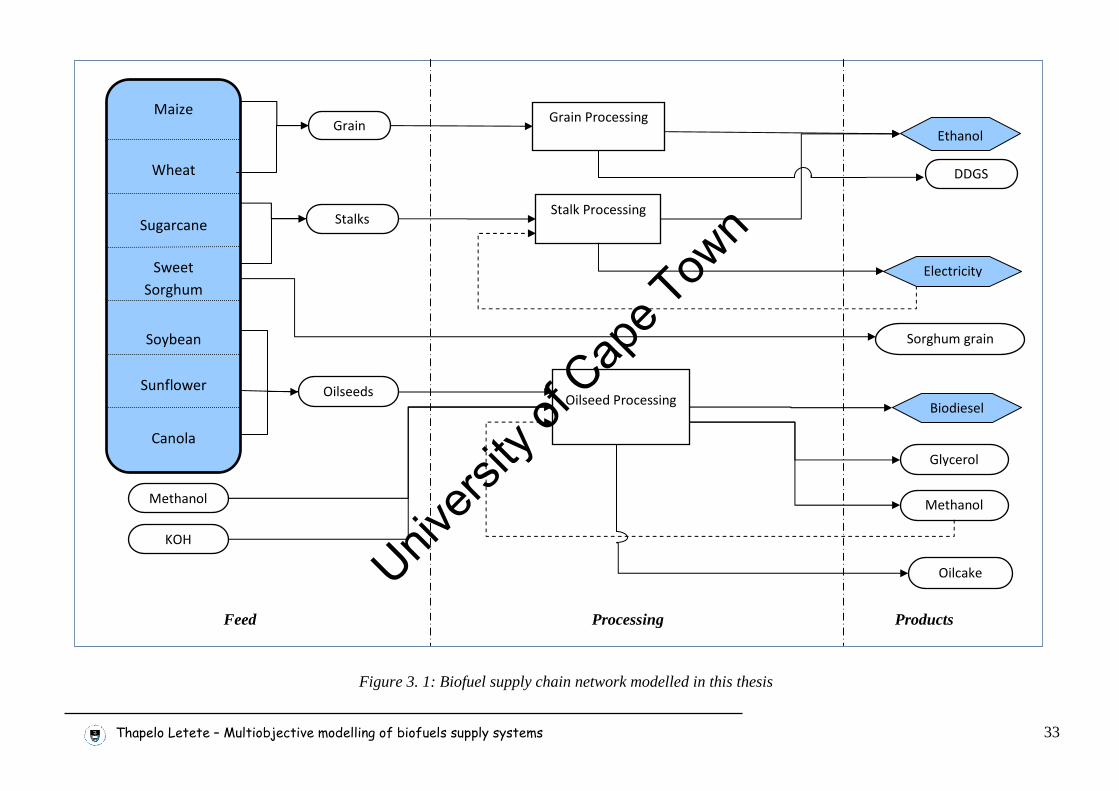
Thapelo Letete – Multiobjective modelling of biofuels supply systems 33
Figure 3. 1: Biofuel supply chain network modelled in this thesis
KOH
Oilseeds
Methanol
Stalks
Oilseed Processing
Oilcake
Glycerol
Methanol
Sorghum grain
Grain
Stalk Processing
Feed Processing Products
Grain Processing
DDGS
Ethanol
Biodiesel
Electricity
Maize
Wheat
Sugarcane
Sweet
Sorghum
Soybean
Sunflower
Canola
Univers
ity of
Cap
e Tow
n
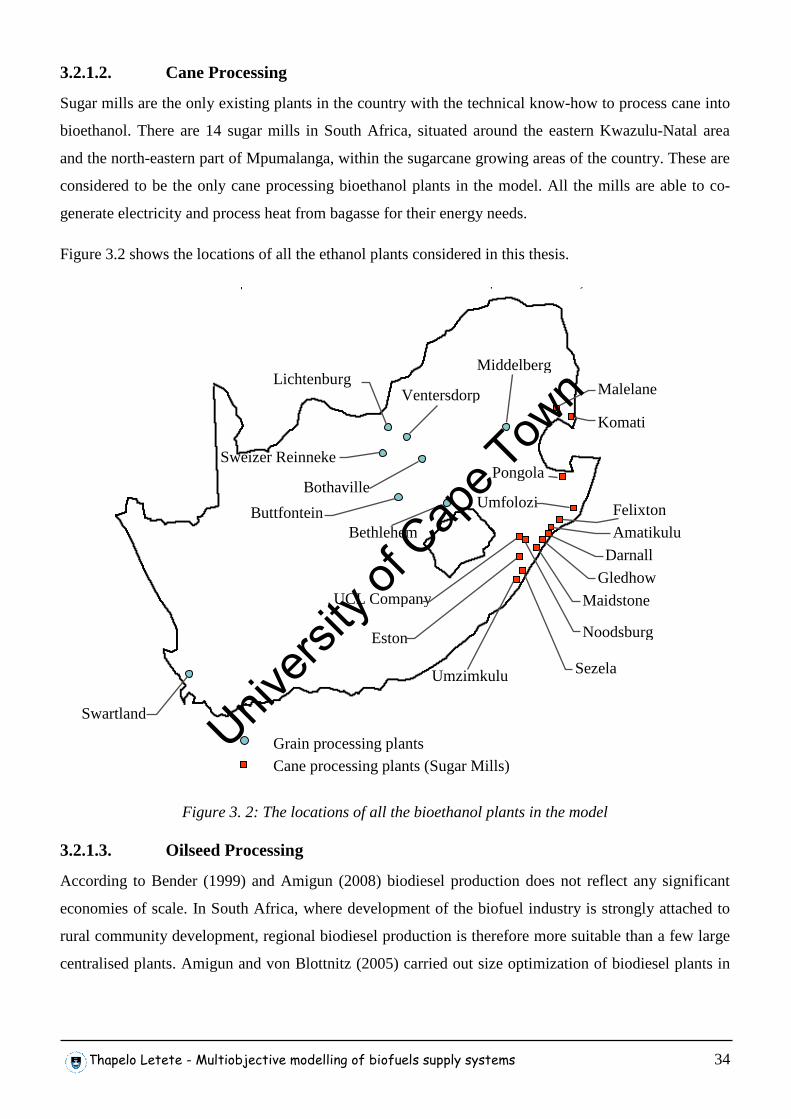
Thapelo Letete - Multiobjective modelling of biofuels supply systems 34
3.2.1.2. Cane Processing
Sugar mills are the only existing plants in the country with the technical know-how to process cane into
bioethanol. There are 14 sugar mills in South Africa, situated around the eastern Kwazulu-Natal area
and the north-eastern part of Mpumalanga, within the sugarcane growing areas of the country. These are
considered to be the only cane processing bioethanol plants in the model. All the mills are able to co-
generate electricity and process heat from bagasse for their energy needs.
Figure 3.2 shows the locations of all the ethanol plants considered in this thesis.
Figure 3. 2: The locations of all the bioethanol plants in the model
3.2.1.3. Oilseed Processing
According to Bender (1999) and Amigun (2008) biodiesel production does not reflect any significant
economies of scale. In South Africa, where development of the biofuel industry is strongly attached to
rural community development, regional biodiesel production is therefore more suitable than a few large
centralised plants. Amigun and von Blottnitz (2005) carried out size optimization of biodiesel plants in
Grain processing plants
Cane processing plants (Sugar Mills)
Malelane
Komati
Pongola
Umfolozi Buttfontein
Bothaville
Sweizer Reinneke
Ventersdorp
Swartland
Lichtenburg Middelberg
Maidstone
Darnall
Gledhow
Amatikulu
Felixton
Bethlehem
Sezela Umzimkulu
Noodsburg Eston
UCL Company
Univers
ity of
Cap
e Tow
n
Thapelo Letete - Multiobjective modelling of biofuels supply systems 35
South Africa using Jatropha curcas as feedstock and concluded that the optimal plant size lies in the
range of 1500 kg/hr – 3500 kg/hr.
The specifications of oilseed processing plants modelled in this thesis were based on a scenario
presented by Nolte (2007): Assuming an optimal plant size of 2500 kg/hr, Nolte proposes the use of
containerized biodiesel plants manufactured by a Dutch biodiesel equipment specialist, BioKing®, with
production capacities of 2640 kg/hr. These plants consist of 20 tonne/hr hexane oil extractors,
transesterification systems and batch glycerol purifiers (Appendix A).
Other specific properties of the plants are summarized below:
1. They are small and relatively easy to move around
2. They are fitted with continuous transesterification reactors with high yields and fast reaction
times
3. For biodiesel/glycerol separation centrifuges are used, thereby speeding up the whole process
4. The methanol obtained from the glycerol purifier can be recycled to reduce processing costs
5. Only the hexane extractor is powered by electricity while the rest of the plant is fitted with a
burner and generator that run on some of the biodiesel and glycerol produced by the plant.
In this thesis it is assumed that each biodiesel plant can adequately service one local municipal area, and
it can either be permanently located at centre of the municipal agricultural area or periodically be moved
between two or three oilseed-growing areas within the municipality.
3.2.2. Bioenergy Crops
Seven bioenergy crops have been considered in this thesis; two grains, two sugar crops and three
oilseeds. This section discusses all these crops in detail.
3.2.2.1. Maize
Maize is the most important grain crop in the Southern African Development Community (SADC),
being the primary feed grain for animals and a staple food for people. South Africa is by far the largest
producer of maize in the continent with an average production of 8.5 million tonnes per year between
1993 and 2007. About 60% of maize produced in South Africa is white and the remainder is yellow
maize (DoA, 2006).
For food security purposes the National Industrial Biofuels Strategy (DME, 2007) excludes the use of
maize to produce bioethanol in the initial phases of the biofuels industry development. The strategy
Univers
ity of
Cap
e Tow
n
Thapelo Letete - Multiobjective modelling of biofuels supply systems 36
further states that this restraint on maize will only be lifted once “certainty on the ability of the current
underutilized land to produce has been ascertained and the necessary measures are in place to guard
against extreme food inflation”.
The focus of this thesis is solely on the use of currently underutilized land dedicated to biofuels
production, and therefore it is not inappropriate to include maize in the model. It was assumed that only
yellow maize is dedicated to bioethanol production.
3.2.2.2. Wheat
Wheat is the third most important field crop in South Africa, after maize and sugarcane, in terms of
value of production. As a staple food, however, wheat is only surpassed by maize in importance,
especially in the rapidly urbanizing areas of the country. In South Africa wheat is produced primarily for
human consumption with only small quantities of poorer quality wheat used as animal feed. Before the
1970’s wheat was only produced in the winter rainfall area of the Cape but has since been grown in the
Free State and other parts of the country (FPM, 2004). In the Western Cape, wheat remains the primary
grain of focus for bioethanol production, while other feedstocks under consideration include triticale,
barley and other forage crops grown in smaller quantities.
3.2.2.3. Sugarcane
South Africa used ethanol produced from sugarcane as fuel for automobiles as early as the 1920’s
through to the 1960’s when the world saw the emergence of cheap and abundant crude petroleum oil.
The South African sugarcane growing industry is composed of approximately 50 000 registered cane
growers who produce some 20 million tons of sugarcane per annum in areas around the 14 sugar mills,
extending from the Eastern Cape through kwaZulu-Natal to the subtropical area of Mpumalanga (FPM,
2004). Although the South African Sugar Industry produces some by-products, the industry has sugar as
its only significant commercial product, which makes it susceptible to fluctuations in the world sugar
market (Wienese and Purchase, 2004). According to the first national biofuels report (Germishuis,
2006), the production of ethanol from sugarcane “has the potential to enhance the sustainability of the
sugar industry in South Africa and to stimulate growth both industrially and agriculturally in the areas
where the industry operates”. Sugarcane is one of the two crops specifically targeted by the national
Biofuels Industry Strategy to drive the bioethanol industry in South Africa.
3.2.2.4. Sweet Sorghum
Sorghum is a C4 crop which finds its origins in the central-eastern part of Africa. Sorghums are drought
resistant crops, making them favourable for growth in semi-arid areas where maize would not thrive
Univers
ity of
Cap
e Tow
n
Thapelo Letete - Multiobjective modelling of biofuels supply systems 37
(Grassi, 2001). Sorghums are generally classified as grain sorghum, fibre sorghum and sweet sorghum
depending on their characteristics and use.
In South Africa grain sorghum is the only type of sorghum produced commercially, mainly cultivated on
low-potential, shallow soils with high clay content in the Free State, Limpopo, Mpumalanga and North
West provinces. Although it is the third most important grain in the country, after maize and wheat,
grain sorghum only contributes a small percentage to the total domestic grains. Sorghum grain is mainly
used for human consumption and the animal market serves as an outlet channel for surpluses since
sorghum can be used to successfully substitute maize as an energy source (FPM, 2004).
Sweet sorghum is similar to grain sorghum but features more rapid growth, higher biomass production,
wider adaptation and, most importantly, higher sugar content in the stalk (Reddy, 2007). The latter
characteristic makes sweet sorghum well suited for making sugar in China and liquid food sweeteners in
India. In Southern Africa the juicy sweet sorghum stems are used in the food market as snack (Balole,
2001). Sweet sorghum is seen as the most versatile field crop for its ability to produce multiple products
at the same time: grain for human consumption from its ear-head, sugary juice and bagasse from its stalk
and also green foliage that can be used as fodder for animals. This characteristic of sweet sorghum has
seen it gain world attention as a promising bioenergy crop and alternative raw material for the
production of ethanol (TNAU, 2007). Since 1983, research has been undertaken in China, India and,
more recently, Australia to breed and test new hybrids of sweet sorghum for use as raw material in
ethanol production (Gnansounou et al., 2005;ICRISAT, 2006;Hallam, 2007).
This thesis looks at a scenario where South African farmers use their experience with grain sorghum to
grow sweet sorghum for ethanol production. The modelled system assumes that only the sorghum stalk
is used for ethanol production while the grain is directed to the food market in an attempt to address
food security as opposed to threatening it.
3.2.2.5. Soybean
Soybean is a relatively difficult crop to grow, ideally requiring warm, fertile clayish soils. In South
Africa, the crop is mainly grown in Mpumalanga, the Free State and Kwazulu-Natal with small
quantities cultivated in the other north-eastern provinces. The main use of soybean in South Africa is in
the animal feed market. Over a period of 10 years the production of soybean in the country increased 5-
fold, from 80 000 tonnes in 1996 to 424 000 tonnes in 2006. This increase is attributed to the growing
interest in soy products by South Africans because of the associated health benefits, and also the
farmers’ view of soybean as an economical replacement for maize and a crop for the future (FPM,
2004).
Univers
ity of
Cap
e Tow
n
Thapelo Letete - Multiobjective modelling of biofuels supply systems 38
The world’s largest producer of Coal-to-liquid fuels, SASOL, has shown interest in building a 400 000
ton/yr soybean fed biodiesel plant. According to Prasad and Visagie (2005) soy appears to be the most
appropriate crop because, apart from the oil used for making biodiesel, it also produces soymeal as by-
product. The latter is needed by both the animal feed and human consumption markets for alleviating
protein deficiency.
3.2.2.6. Sunflower seed
The primary use of sunflower seed in South Africa is in the production of oil and oilcake for human and
animal consumption respectively. Because of its relatively high resistance to drought, sunflower is
mainly grown in the marginal production areas of the Free State and North West Province. Sunflower
seed is the major source of plant oil for human consumption in the country, with local production
meeting only about half the national demand while the balance is made up of imports and other locally
produced oil seeds. The demand for sunflower seed is strongly dependant on the demand for its oilcake
because, unlike soymeal, sunflower meal is characterized by a high fibre content which restricts its
inclusion in pig and poultry feeds (FPM, 2004).
The national Biofuels Industrial Strategy proposes the use of sunflower seed as a major feedstock,
together with soybean and canola, for the development of a local biodiesel industry.
3.2.2.7. Canola
Canola refers to genetically selected and nutritionally superior rapeseed that contains oil with less than
2% ericic acid and less than 30 µmol/g aliphatic glucosinulates (Tesfamariam, 2004). In South Africa,
canola is mainly grown in the Western Cape Province, although since 2001, small quantities have also
been planted in the northern parts of the country. In the wheat producing areas of the Western and
Southern Cape, canola is becoming increasingly important for crop rotation as it provides a disease
break for cereal crops and allows the use of alternative weed and pest control chemicals while also
diversifying farm income (Hardy et al., 2004). Canola competes with other oilseeds both in the human
consumption and the animal feed markets. The unique fatty acid composition of canola oil, however,
provides a niche market for it as a healthier choice for human consumption, thus it is expected that its
consumption in the human market will continue to rise (FPM, 2004).
As the major oilseed grown in the Western and southern Cape, canola has become the primary focus for
biodiesel production in these areas and there are several private companies looking to explore this new
energy venture. The Biodiesel centre, housed in Bellville in greater Cape Town, is one such organization
which is currently conducting tests and creating awareness on the use of canola for biodiesel production.
Univers
ity of
Cap
e Tow
n
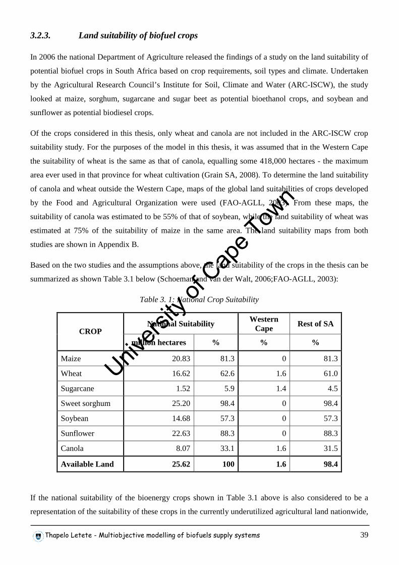
Thapelo Letete - Multiobjective modelling of biofuels supply systems 39
3.2.3. Land suitability of biofuel crops
In 2006 the national Department of Agriculture released the findings of a study on the land suitability of
potential biofuel crops in South Africa based on crop requirements, soil types and climate. Undertaken
by the Agricultural Research Council’s Institute for Soil, Climate and Water (ARC-ISCW), the study
looked at maize, sorghum, sugarcane and sugar beet as potential bioethanol crops, and soybean and
sunflower as potential biodiesel crops.
Of the crops considered in this thesis, only wheat and canola are not included in the ARC-ISCW crop
suitability study. For the purposes of the model in this thesis, it was assumed that in the Western Cape
the suitability of wheat is the same as that of canola, equalling some 418,000 hectares - the maximum
area ever used in that province for wheat cultivation (Grain SA, 2008). To determine the land suitability
of canola and wheat outside the Western Cape, maps of the global land suitabilities of crops developed
by the Food and Agricultural Organization were used (FAO-AGLL, 2003). From these maps, the
suitability of canola was estimated to be 55% of that of soybean, while the land suitability of wheat was
estimated at 75% of the suitability of maize in the same area. The land suitability maps from both
studies are shown in Appendix B.
Based on the two studies and the assumptions above, the land suitability of the crops in the thesis can be
summarized as shown Table 3.1 below (Schoeman and van der Walt, 2006;FAO-AGLL, 2003):
Table 3. 1: National Crop Suitability
National Suitability Western Cape
Rest of SA CROP
million hectares % % %
Maize 20.83 81.3 0 81.3
Wheat 16.62 62.6 1.6 61.0
Sugarcane 1.52 5.9 1.4 4.5
Sweet sorghum 25.20 98.4 0 98.4
Soybean 14.68 57.3 0 57.3
Sunflower 22.63 88.3 0 88.3
Canola 8.07 33.1 1.6 31.5
Available Land 25.62 100 1.6 98.4
If the national suitability of the bioenergy crops shown in Table 3.1 above is also considered to be a
representation of the suitability of these crops in the currently underutilized agricultural land nationwide,
Univers
ity of
Cap
e Tow
n
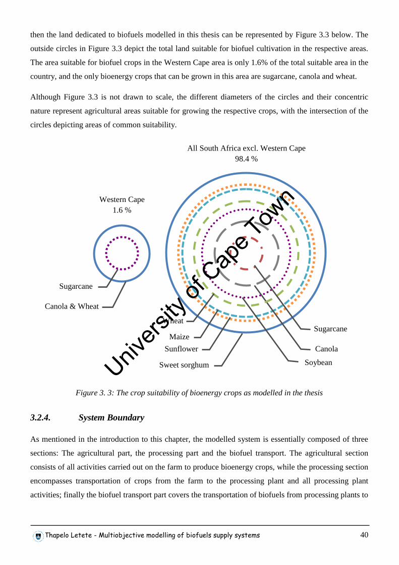
Thapelo Letete - Multiobjective modelling of biofuels supply systems 40
then the land dedicated to biofuels modelled in this thesis can be represented by Figure 3.3 below. The
outside circles in Figure 3.3 depict the total land suitable for biofuel cultivation in the respective areas.
The area suitable for biofuel crops in the Western Cape area is only 1.6% of the total suitable area in the
country, and the only bioenergy crops that can be grown in this area are sugarcane, canola and wheat.
Although Figure 3.3 is not drawn to scale, the different diameters of the circles and their concentric
nature represent agricultural areas suitable for growing the respective crops, with the intersection of the
circles depicting areas of common suitability.
Figure 3. 3: The crop suitability of bioenergy crops as modelled in the thesis
3.2.4. System Boundary
As mentioned in the introduction to this chapter, the modelled system is essentially composed of three
sections: The agricultural part, the processing part and the biofuel transport. The agricultural section
consists of all activities carried out on the farm to produce bioenergy crops, while the processing section
encompasses transportation of crops from the farm to the processing plant and all processing plant
activities; finally the biofuel transport part covers the transportation of biofuels from processing plants to
Western Cape 1.6 %
All South Africa excl. Western Cape 98.4 %
Canola & Wheat
Soybean
Canola
Sweet sorghum
Sunflower
Sugarcane
Maize
Sugarcane
Wheat
Univers
ity of
Cap
e Tow
n
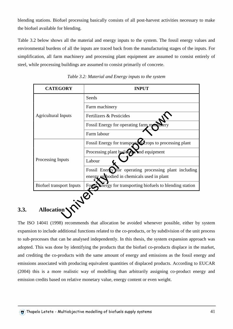
Thapelo Letete - Multiobjective modelling of biofuels supply systems 41
blending stations. Biofuel processing basically consists of all post-harvest activities necessary to make
the biofuel available for blending.
Table 3.2 below shows all the material and energy inputs to the system. The fossil energy values and
environmental burdens of all the inputs are traced back from the manufacturing stages of the inputs. For
simplification, all farm machinery and processing plant equipment are assumed to consist entirely of
steel, while processing buildings are assumed to consist primarily of concrete.
Table 3.2: Material and Energy inputs to the system
CATEGORY INPUT
Seeds
Farm machinery
Fertilizers & Pesticides
Fossil Energy for operating farm machinery
Agricultural Inputs
Farm labour
Fossil Energy for transporting crops to processing plant
Processing plant buildings and equipment
Labour Processing Inputs
Fossil Energy for operating processing plant including energy embodied in chemicals used in plant
Biofuel transport Inputs Fossil Energy for transporting biofuels to blending station
3.3. Allocation
The ISO 14041 (1998) recommends that allocation be avoided whenever possible, either by system
expansion to include additional functions related to the co-products, or by subdivision of the unit process
to sub-processes that can be analysed independently. In this thesis, the system expansion approach was
adopted. This was done by identifying the products that the biofuel co-products displace in the market,
and crediting the co-products with the same amount of energy and emissions as the fossil energy and
emissions associated with producing equivalent quantities of displaced products. According to EUCAR
(2004) this is a more realistic way of modelling than arbitrarily assigning co-product energy and
emission credits based on relative monetary value, energy content or even weight.
Univers
ity of
Cap
e Tow
n
Thapelo Letete - Multiobjective modelling of biofuels supply systems 42
Five types of by-products are produced in the system; DDGS, green electricity, sweet sorghum grain,
oilcakes and glycerol. In this thesis it was assumed that DDGS replaces both soymeal and maize as
animal feed, while green electricity and sweet sorghum grain replace electricity from Eskom and grain
sorghum grown for human consumption respectively. Both sunflower cake and canola cake replace
soymeal as feed for animals. In determining the energy credit and environmental burdens of soymeal,
allocation could not be avoided and therefore mass allocation was employed. It was assumed that
glycerol replaces synthetic glycerine in the world market.
3.4. Model Objectives
The development of a biofuel industry in South Africa is a process that inevitably affects the economic
and social spheres, whilst also impacting on the bio-physical environment. This section identifies and
discusses key economic, social and environmental issues affecting the choice and quantity of bioenergy
crops grown for biofuels production in different areas of the country. For each of the three spheres, the
identified indicator is then defined as an objective for the model.
3.4.1. Economic objective
For investors the return on financial investment of any business venture is the all-important factor that
determines whether or not the investors can take part. In the biofuel industry the key economic indicator
is value added by the biofuel producer, which can be defined as:
Value Added = (Biofuel revenue + By-product revenue) – (Raw material cost + processing cost).
Here the processing cost includes the cost of all consumables, energy and labour at the processing plant
and all transportation costs. In this thesis it was assumed that processing plants buy crops from farmers
at market prices and sell the biofuels and by-products at market prices as well.
For modelling at national level the economic objective as thus described – focusing only on processing
plant value addition – was deemed appropriate as it is a common way of assessing the economic
feasibility of biofuel projects (BFAP, 2007). As will be seen in Chapter 5, however, it was no longer
possible at local government level modelling to ignore the other economic benefits associated with
agricultural value addition.
3.4.2. Social objective
The Biofuels Industrial Strategy of South Africa (DME, 2007) reports that the development of a biofuels
industry in South Africa is “driven predominantly by the need to address issues of poverty and economic
Univers
ity of
Cap
e Tow
n
Thapelo Letete - Multiobjective modelling of biofuels supply systems 43
development”; hence the strategy is specifically targeted at “creating jobs in the energy-crop and
biofuels value chain, and to act as a bridge between the first and second economy.” This implies that
job-creation is the single most important social objective to be monitored in any biofuel project in the
country.
This thesis focuses only on the direct jobs created within both the agricultural and the processing
sections of the biofuels supply chain, and does not consider any jobs created outside the supply chain as
a result of the production of biofuels as shown in the following equation:
Job-creation = Agricultural Jobs-Permanent + Agricultural jobs-Temporary + Processing Jobs
3.4.3. Environmental objective
Although South Africa does not have quantified greenhouse gas emission reduction targets during this
first commitment period of the Kyoto protocol, many of the proposals for a post-2012 climate action
plan support emission reduction commitments for many developing countries including South Africa. In
the very least South Africa will be obliged to make and implement low-carbon sustainable development
policies. This means that the carbon dioxide emissions reduction capacity of any bioenergy venture in
the country is important in determining its long-term relevance and importance to the country’s targets
and goals.
The emission reduction capacity of a biofuel supply chain can be expressed as the Avoided greenhouse
gas emissions, defined as: The difference of the greenhouse gas emissions that would have resulted from
the production, transportation and use of the products that are replaced by all biomass products (biofuels
and by-products) and the greenhouse gas emissions released as a result of producing the biofuels.
Avoided GHG emissions = GHG emissions-Replaced products – GHG emissions-Biofuel production
3.5. Problem Formulation
The problem is set up as a multi-objective optimization problem, maximizing economic gain, avoided
greenhouse gas emissions and the number of jobs created within the supply chain. The basis of the
analysis is one hectare of available land dedicated to biofuels production.
In the analysis, two approaches addressing two different key questions are adopted:
In the first approach, the problem is formulated to compare all crops and to determine the overall
optimum crop or combination of crops based on the economic, social and environmental objectives
selected. Given one hectare of currently underutilized agricultural land, this approach seeks to determine
Univers
ity of
Cap
e Tow
n
Thapelo Letete - Multiobjective modelling of biofuels supply systems 44
which biofuel crop (and subsequently biofuel) offers the most benefits. A sensitivity analysis of this
approach is also useful in establishing the key variables that determine the preference of one biofuel
over the other.
The second approach serves to determine a combination of crops that result in optimal land use, based
on the selected objectives, to achieve the 2% biodiesel and 8% bioethanol market penetration target
proposed by the Biofuels Industrial Strategy of South Africa. In this approach the comparison is solely
on the crops competing for the production of the same type of biofuel.
It must be noted that the model objectives as described in section 3.4 above have different system
boundaries; while the economic objective is focused on processing plant value addition, the
environmental and social objectives look at cradle-to-grave emissions and farm-to-blending station job
creation respectively. Full cradle-to-grave analyses for all three objectives would be ideal, but because
of the complexities associated with full social and economic life-cycle analyses and the scarcity of data
for such analyses, it was not possible to do the full cradle-to-grave analyses for them.
3.6. Objective Equations
In this section, the model objectives outlined in section 3.4 are translated into mathematical equations
that can readily be formulated into multi-objective optimization problems.
3.6.1. Maximisation of Economic gain
In section 3.4.1 the Economic Gain or Value added V(x) is defined as:
Value Added = (Biofuel revenue + By-product revenue) – (Raw material cost + processing cost).
If I and J are sets of biofuels and biofuel crops respectively, defined as follows:
i Є I = {Biodiesel, Bioethanol}
j Є J= { Maize, Wheat, Sugarcane, Sweet sorghum, Soybean, Sunflower, Canola}
then the economic gain can be expressed in R/ha/yr as
where
= Fraction of Land occupied by bioenergy crop j
= Yield of biofuel i produced from bioenergy crop j [litres/hectare/yr]
Univers
ity of
Cap
e Tow
n
Thapelo Letete - Multiobjective modelling of biofuels supply systems 45
= = = = 0
= = =0
= Selling price of biofuel i [R/litre]
= Selling price of by-product of bioenergy crop j [R/kg]
= price of electricity [R/kWh]
= Market price of crop j [R/tonne]
= All post-harvest costs of processing crop j [R/litre]
= Amount of by-product produced per litre of biofuel from crop j [kg/litre]
= tonnes of crop j required to produce a litre of biofuel [tonne/litre]
= Amount of excess co-generated electricity from crop j [kWh/ha].
3.6.2. Maximisation of Avoided Greenhouse gas emissions
As outlined in section 3.4.2, Avoided greenhouse gas emissions, G(x), is defined as an objective
function as:
Avoided GHG emissions = GHG emissions-Replaced products – GHG emissions-Biofuel production.
Three types of emissions resulting from biofuel production have been identified:
i. CO2 emissions from direct consumption of fossil fuels in agricultural and processing operations,
including transportation of energy crops and transportation of biofuels. (Direct fossil fuel
emissions)
ii. CO2 emitted during the production and transportation of all chemicals, fertilizers, steel used for
making agricultural implements and processing plant equipment, concrete used for industrial
buildings, fossil fuels, electricity and seeds. (Indirect fossil fuel emissions)
iii. Emissions that are not related to fossil energy use, comprising of CH4 and N2O emissions from
the burning of sugarcane trash before harvesting, and CO2 and N2O emissions from the soil as a
result of fertilizer and lime application. (Non-fossil fuel emissions)
Figure 3.4 below shows all the greenhouse gas emissions from biofuel production.
Univers
ity of
Cap
e Tow
n
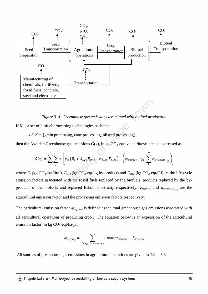
Thapelo Letete - Multiobjective modelling of biofuels supply systems 46
Figure 3. 4: Greenhouse gas emissions associated with biofuel production
If K is a set of biofuel processing technologies such that
k Є K = {grain processing, cane processing, oilseed processing}
then the Avoided Greenhouse gas emissions G(x), in kg CO2-equivalent/ha/yr, can be expressed as
where Ei (kg CO2-eqt/litre), EBPj (kg CO2-eqt/kg by-product) and Eelec (kg CO2-eqt/GJ)are the life-cycle
emission factors associated with the fossil fuels replaced by the biofuels, products replaced by the by-
products of the biofuels and replaced Eskom electricity respectively. and are the
agricultural emission factor and the processing emission factors respectively.
The agricultural emission factor is defined as the total greenhouse gas emissions associated with
all agricultural operations of producing crop j. The equation below is an expression of the agricultural
emission factor, in kg CO2-eqt/ha/yr:
All sources of greenhouse gas emissions in agricultural operations are given in Table 3.3.
Seed Transportation
Biofuel Transportation
Transportation Manufacturing of chemicals, fertilizers, fossil fuels, concrete, steel and electricity
Seed preparation
CO2
Crop Transportation
CO2, N2O, CH4,
CO2
CO2
CO2 CO2 CO2
CO2
Agricultural operations
Biofuel production
Univers
ity of
Cap
e Tow
n

Thapelo Letete - Multiobjective modelling of biofuels supply systems 47
Table 3. 3: Sources of emissions in agricultural operations
Units Source
Amount E (Emission factor)
Seed kg/ha Kg CO2-eqt/kg
Diesel GJ/ha Kg CO2-eqt/GJ
Nitrogen kg/ha Kg CO2-eqt/kg
P2O5 kg/ha Kg CO2-eqt/kg
K2O kg/ha Kg CO2-eqt/kg
Lime kg/ha Kg CO2-eqt/kg
Herbicides kg/ha Kg CO2-eqt/kg
Pesticides kg/ha Kg CO2-eqt/kg
Fungicides kg/ha Kg CO2-eqt/kg
Trash burning kg trash/ha Kg CO2-eqt/kg trash
Agricultural machinery kg steel/ha Kg CO2-eqt/kg steel
Agricultural labour Persons/ha Kg CO2-eqt/person
is an aggregation of all post-harvest emissions associated with the production of biofuel i
from crop j. Expressed in kg CO2-eqt/litre/yr, the processing emission factor is given by
where
= emission factor of chemicals used in processing plant k [kgCO2-eqt/litre biofuel]
= emission factor of fossil energy used in plant k [kgCO2-eqt/litre biofuel]
= emission factor associated with transportation of crop j [kg CO2-eqt/ton crop]
= emission factor of transporting biofuel i [kg CO2-eqt/litre biofuel]
= emission factor associated with human labour [kg CO2-eqt/person]
= emission factor associated with steel [kg CO2-eqt/kg steel]
= emission factor associated with concrete [kg CO2-eqt/kg concrete]
= labour requirements of processing technology k [persons/litre biofuel]
Univers
ity of
Cap
e Tow
n
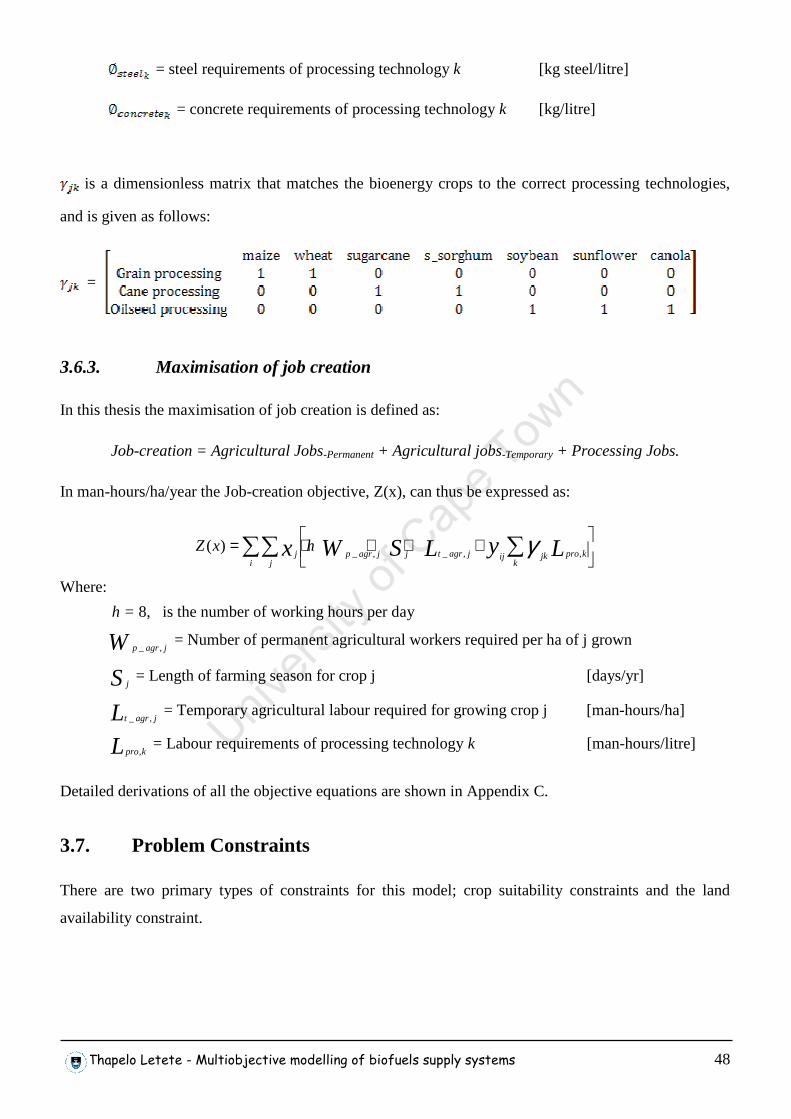
Thapelo Letete - Multiobjective modelling of biofuels supply systems 48
= steel requirements of processing technology k [kg steel/litre]
= concrete requirements of processing technology k [kg/litre]
is a dimensionless matrix that matches the bioenergy crops to the correct processing technologies,
and is given as follows:
=
3.6.3. Maximisation of job creation
In this thesis the maximisation of job creation is defined as:
Job-creation = Agricultural Jobs-Permanent + Agricultural jobs-Temporary + Processing Jobs.
In man-hours/ha/year the Job-creation objective, Z(x), can thus be expressed as:
∑∑ ∑
++⋅⋅=i j k
kprojkijjagrtjjagrpj LyLSWx hxZ,,_,_
)( γ
Where:
h = 8, is the number of working hours per day
W jagrp ,_ = Number of permanent agricultural workers required per ha of j grown
Sj = Length of farming season for crop j [days/yr]
L jagrt ,_ = Temporary agricultural labour required for growing crop j [man-hours/ha]
L kpro, = Labour requirements of processing technology k [man-hours/litre]
Detailed derivations of all the objective equations are shown in Appendix C.
3.7. Problem Constraints
There are two primary types of constraints for this model; crop suitability constraints and the land
availability constraint.
Univers
ity of
Cap
e Tow
n
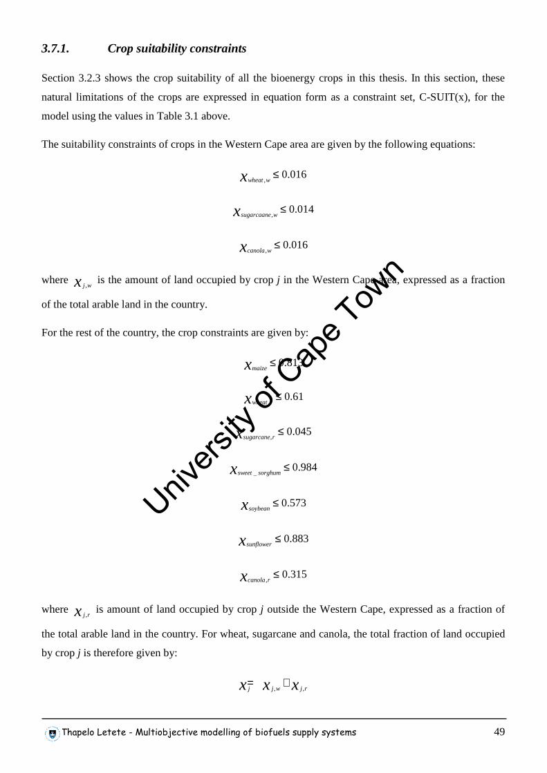
Thapelo Letete - Multiobjective modelling of biofuels supply systems 49
3.7.1. Crop suitability constraints
Section 3.2.3 shows the crop suitability of all the bioenergy crops in this thesis. In this section, these
natural limitations of the crops are expressed in equation form as a constraint set, C-SUIT(x), for the
model using the values in Table 3.1 above.
The suitability constraints of crops in the Western Cape area are given by the following equations:
016.0,
≤x wwheat
014.0,
≤x wsugarcaane
016.0,
≤x wcanola
where x wj , is the amount of land occupied by crop j in the Western Cape area, expressed as a fraction
of the total arable land in the country.
For the rest of the country, the crop constraints are given by:
813.0≤xmaize
61.0,
≤x rwheat
045.0,
≤x rsugarcane
984.0_
≤x sorghumsweet
573.0≤xsoybean
883.0≤xsunflower
315.0,
≤x rcanola
where x rj , is amount of land occupied by crop j outside the Western Cape, expressed as a fraction of
the total arable land in the country. For wheat, sugarcane and canola, the total fraction of land occupied
by crop j is therefore given by:
xxx rjwjj ,,+=
Univers
ity of
Cap
e Tow
n
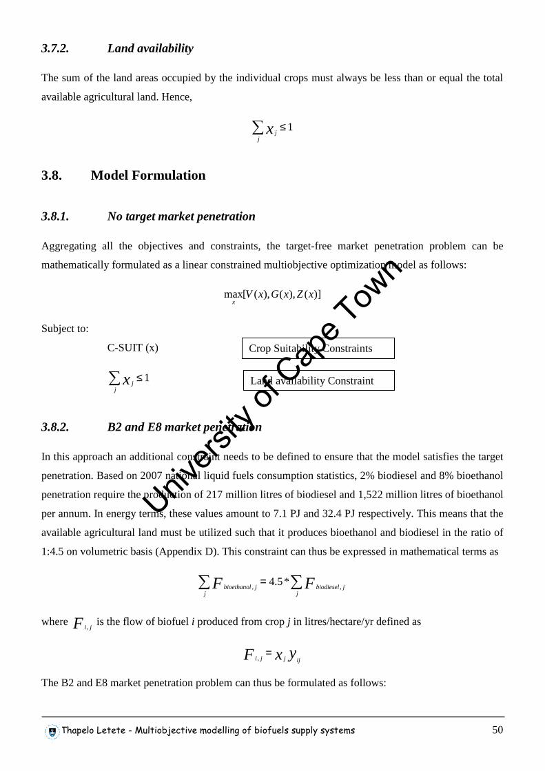
Thapelo Letete - Multiobjective modelling of biofuels supply systems 50
3.7.2. Land availability
The sum of the land areas occupied by the individual crops must always be less than or equal the total
available agricultural land. Hence,
∑ ≤j
jx 1
3.8. Model Formulation
3.8.1. No target market penetration
Aggregating all the objectives and constraints, the target-free market penetration problem can be
mathematically formulated as a linear constrained multiobjective optimization model as follows:
)](),(),([max xZxGxVx
Subject to:
C-SUIT (x)
∑ ≤j
jx 1
3.8.2. B2 and E8 market penetration
In this approach an additional constraint needs to be defined to ensure that the model satisfies the target
penetration. Based on 2007 national liquid fuels consumption statistics, 2% biodiesel and 8% bioethanol
penetration require the production of 217 million litres of biodiesel and 1,522 million litres of bioethanol
per annum. In energy terms, these values amount to 7.1 PJ and 32.4 PJ respectively. This means that the
available agricultural land must be utilized such that it produces bioethanol and biodiesel in the ratio of
1:4.5 on volumetric basis (Appendix D). This constraint can thus be expressed in mathematical terms as
∑ ∑=j j
jbiodieseljbioethanol FF ,,*5.4
where F ji , is the flow of biofuel i produced from crop j in litres/hectare/yr defined as
yxF ijjji=
,
The B2 and E8 market penetration problem can thus be formulated as follows:
Crop Suitability Constraints
Land availability Constraint
Univers
ity of
Cap
e Tow
n
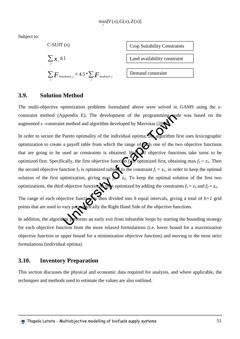
Thapelo Letete - Multiobjective modelling of biofuels supply systems 51
)](),(),([max xZxGxVx
Subject to:
C-SUIT (x)
∑ ≤j
jx 1
∑ ∑=j j
jbiodieseljbioethanol FF ,,*5.4
3.9. Solution Method
The multi-objective optimization problems formulated above were solved in GAMS using the ε-
constraint method (Appendix E). The development of the programming code was based on the
augmented ε -constraint method and algorithm developed by Mavrotas (2007).
In order to secure the Pareto optimality of the individual optima, the algorithm first uses lexicographic
optimization to create a payoff table from which the range of each one of the two objective functions
that are going to be used as constraints is obtained. Here all objective functions take turns to be
optimized first. Specifically, the first objective function f1 is optimized first, obtaining max f1 = z1. Then
the second objective function f2 is optimized subject to the constraint f1 = z1, in order to keep the optimal
solution of the first optimization, giving max f2 = z2. To keep the optimal solution of the first two
optimizations, the third objective function is then optimized by adding the constraints f1 = z1 and f2 = z2.
The range of each objective function is then divided into h equal intervals, giving a total of h+1 grid
points that are used to vary parametrically the Right Hand Side of the objective functions.
In addition, the algorithm performs an early exit from infeasible loops by starting the bounding strategy
for each objective function from the more relaxed formulations (i.e. lower bound for a maximization
objective function or upper bound for a minimization objective function) and moving to the most strict
formulations (individual optima).
3.10. Inventory Preparation
This section discusses the physical and economic data required for analysis, and where applicable, the
techniques and methods used to estimate the values are also outlined.
Crop Suitability Constraints
Land availability constraint
Demand constraint
Univers
ity of
Cap
e Tow
n
Thapelo Letete - Multiobjective modelling of biofuels supply systems 52
3.10.1. Inputs
Average national data were used to determine the physical quantities of the inputs to the system, and
when such information was not available, international data were used, adopting in the preference those
values that best represent the South African situation.
3.10.1.1. Seeds
Based on personal interviews with five maize and soybean farmers in the Eastern Free State, the average
seed application rates of maize and soybean were found to be around 12.5 kg of maize seed per hectare
and 76.1 kg of soybean seed per hectare (Ntholeng, 2008;Ballod, 2008;Macaphasa, 2008;Makoele,
2008). According to the Agricultural Research Council (ARC, 2008), the optimum planting rate of
wheat cultivars in the Cape is about 120 kg per hectare and it was assumed that this is also the case for
the rest of the country. In the absence of local application rates for sweet sorghum and sunflower,
international rates were used in this thesis. For sweet sorghum cultivation an optimal seed rate of 10
kg/ha (TNAU, 2007) was used, while a seed application rate of 3.5 kg/ha was assumed for sunflower
(Kallivroussis et al., 2002) based on agricultural practices in Greece. Hardy et al. (2004) report an
average seeding rate of 4.5 kg/ha of canola in the canola farming areas of the Western Cape.
3.10.1.2. Farm fossil fuel use
Farm fuel energy consists of fossil fuel directly used by farm machinery for ploughing, harrowing,
fertilizing, weed and pest control, sowing and harvesting. In the 2006/2007 farming season, the average
fuel expenses for maize, wheat, soybean and sunflower farming were R505 per ha, R445 per ha, R461
per ha and R439 per ha respectively (Grain SA, 2008). Using the season’s average diesel wholesale
prices of R5.94 per litre for summer grains and R5.83 per litre for winter grains (DME, 2008), the
agricultural fuel use of maize, wheat, soybean and sunflower were calculated to be 85 litres/ha, 78
litres/ha, 76 litres/ha, and 74 litres/ha respectively. Theka (2002) reports a diesel consumption of 88
litres/ha in sugarcane farming in the Kwazulu-Natal province, while Karolina and Hansson (1999)
estimate the diesel consumption for Canola farming at 74 litres/ha based on agricultural practices in
Sweden. In the absence of local data, farm fuel use for sweet sorghum was estimated at 184 litres/ha
using two studies based on agricultural practices in Europe. (Monti and Venturi, 2003;Grassi, 2001)
3.10.1.3. Fertilizers and Agrochemicals
Fertilizer application rates for the cultivation of maize, wheat, sugarcane, soybean and sunflower were
obtained from a study by FAO (2005) on South Africa’s fertilizer usage, while fertilizer application data
relating to canola farming was estimated from conversations with canola farmers in the Western Cape
province (Stephenson, 2007). For sweet sorghum, nitrogen application rates were obtained from a study
Univers
ity of
Cap
e Tow
n
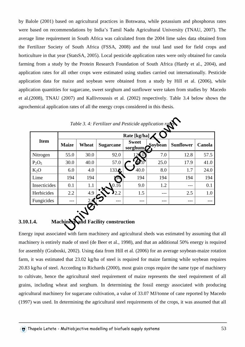
Thapelo Letete - Multiobjective modelling of biofuels supply systems 53
by Balole (2001) based on agricultural practices in Botswana, while potassium and phosphorus rates
were based on recommendations by India’s Tamil Nadu Agricultural University (TNAU, 2007). The
average lime requirement in South Africa was calculated from the 2004 lime sales data obtained from
the Fertilizer Society of South Africa (FSSA, 2008) and the total land used for field crops and
horticulture in that year (StatsSA, 2005). Local pesticide application rates were only obtained for canola
farming from a study by the Protein Research Foundation of South Africa (Hardy et al., 2004), and
application rates for all other crops were estimated using studies carried out internationally. Pesticide
application data for maize and soybean were obtained from a study by Hill et al. (2006), while
application quantities for sugarcane, sweet sorghum and sunflower were taken from studies by Macedo
et al.(2008), TNAU (2007) and Kallivroussis et al. (2002) respectively. Table 3.4 below shows the
agrochemical application rates of all the energy crops considered in this thesis.
Table 3. 4: Fertilizer and Pesticide application rates
Rate [kg/ha] Item
Maize Wheat Sugarcane Sweet sorghum
Soybean Sunflower Canola
Nitrogen 55.0 30.0 92.0 120.0 7.0 12.8 57.5
P2O5 30.0 40.0 57.0 40.0 25.0 17.9 41.0
K2O 6.0 4.0 133.0 40.0 8.0 1.7 24.0
Lime 194 194 194 194 194 194 194
Insecticides 0.1 1.1 0.16 9.0 1.2 --- 0.1
Herbicides 2.2 4.9 2.2 1.5 --- 2.5 1.0
Fungicides --- 2.0 --- --- --- --- ---
3.10.1.4. Machinery and Facility construction
Energy input associated with farm machinery and agricultural sheds was estimated by assuming that all
machinery is entirely made of steel (de Beer et al., 1998), and that an additional 50% energy is required
for assembly (Graboski, 2002). Using data from Hill et al. (2006) for an average soybean-maize rotation
farm, it was estimated that 23.02 kg/ha of steel is required for maize farming while soybean requires
20.83 kg/ha of steel. According to Richards (2000), most grain crops require the same type of machinery
to cultivate, hence the agricultural steel requirement of maize represents the steel requirement of all
grains, including wheat and sorghum. In determining the fossil energy associated with producing
agricultural machinery for sugarcane cultivation, a value of 33.07 MJ/tonne of cane reported by Macedo
(1997) was used. In determining the agricultural steel requirements of the crops, it was assumed that all
Univers
ity of
Cap
e Tow
n
Thapelo Letete - Multiobjective modelling of biofuels supply systems 54
farm machinery is used for 15 years on an average farm of 164 hectares. The latter was calculated from
the number of cultivated crop fields in South Africa and the total land they occupy (DoA, 2007).
According to Hill et al. (2006) buildings of the processing plants are mostly composed of concrete,
while all industrial processing equipment is made entirely of steel. Considering a 20-year life span for
all facilities, Hill calculated the concrete requirements of grain processing plants to be 6.23 g/litre of
bioethanol and the steel requirements to be 0.67 g/litre of bioethanol. For oilseed processing plants these
values are 8.83 and 1.08 g/litre of biodiesel respectively. For cane processing facility construction, the
concrete and steel requirements are 5.11 g/litre and 1.53 g/litre respectively (Macedo et al., 2008).
Detailed facility construction energy requirements are presented in Appendix G.
3.10.1.5. Farm and biofuel labour
Personal interviews with five farm owners in the Eastern Free State show that 8 permanent workers are
required on average per every 1000 hectares in grain and oilseed farms (Macaphasa, 2008;Makoele,
2008;Moloi, 2008;Ntholeng, 2008). For sugarcane, an award-winning sugarcane farmer in Mpumalanga
reports an optimal permanent labour requirement of about 8 workers per 100 hectares (Khosa, 2007).
Hill et al. (2006) reports average post-harvest labour requirements of 4.24 x 10⁻⁷ workers per litre of
grain ethanol and 3.05 x 10⁻⁶ workers per litre of biodiesel, while cane ethanol requires about 1.54 x 10⁻⁶
according to Ometto et al.(2004). The latter values include workers required at the processing plants and
those labourers involved in transportation of feed materials and transportation of the biofuels
themselves.
3.10.1.6. Transportation
The average crop transportation distances were determined based on crop area suitability values shown
in section 3.2.3 and the number of appropriate processing plants available in that area. For maize and
wheat, the average crop transportation return distances are about 196 km and 160 km respectively. On
average the transportation distance for sweet sorghum was found to be 558 km. Assuming that each
biodiesel plant only processes oilseeds grown within one local municipal area, then the return distance
for soybean, sunflower and canola was estimated at 74 km. Detailed distance calculations are shown in
Appendix F.
Regional blending and distributing stations are assumed to be located within 250 km diameters of all
processing plants. It was assumed that all transportation over return distances shorter than 250 km can
be done using a rented 10 ton truck, while all others are done by train.
Univers
ity of
Cap
e Tow
n
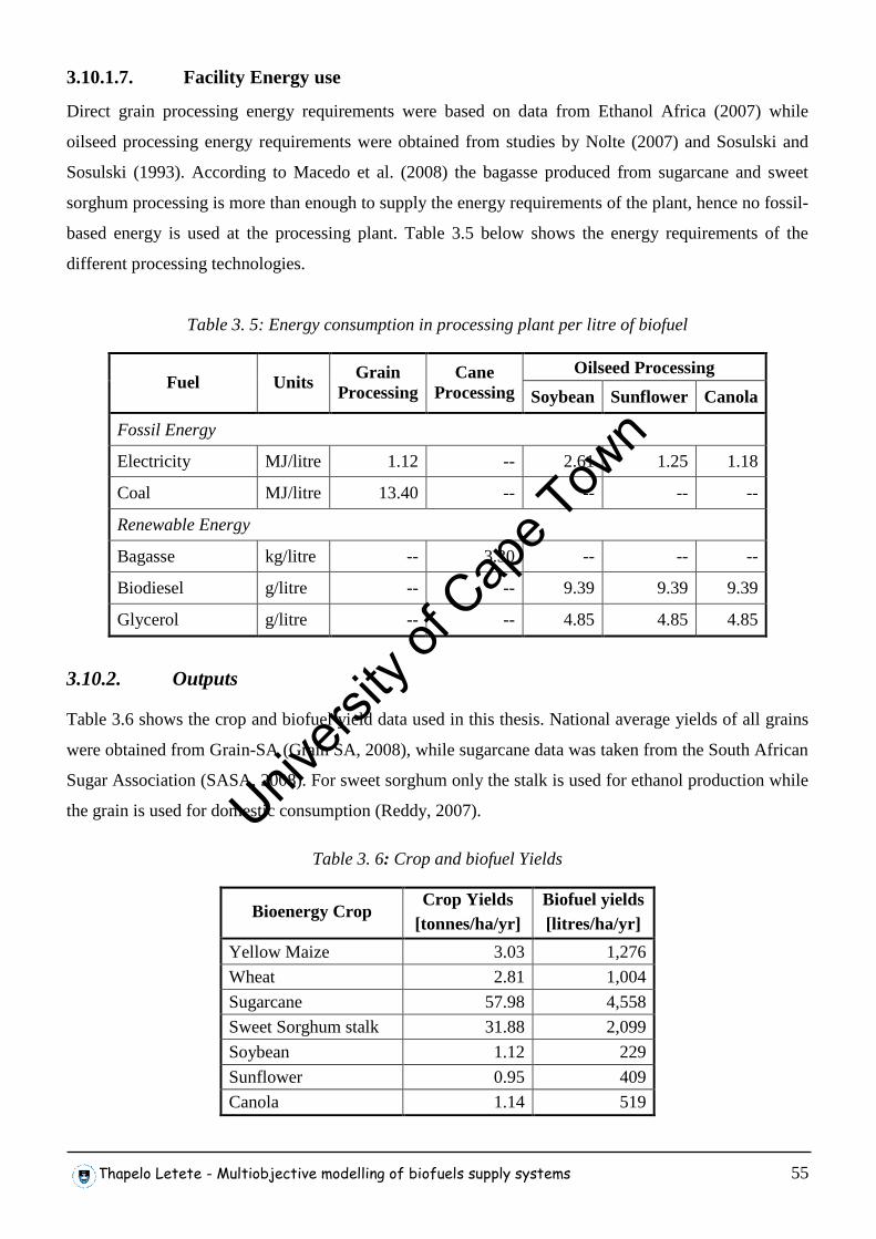
Thapelo Letete - Multiobjective modelling of biofuels supply systems 55
3.10.1.7. Facility Energy use
Direct grain processing energy requirements were based on data from Ethanol Africa (2007) while
oilseed processing energy requirements were obtained from studies by Nolte (2007) and Sosulski and
Sosulski (1993). According to Macedo et al. (2008) the bagasse produced from sugarcane and sweet
sorghum processing is more than enough to supply the energy requirements of the plant, hence no fossil-
based energy is used at the processing plant. Table 3.5 below shows the energy requirements of the
different processing technologies.
Table 3. 5: Energy consumption in processing plant per litre of biofuel
Oilseed Processing Fuel Units Grain
Processing Cane
Processing Soybean Sunflower Canola
Fossil Energy
Electricity MJ/litre 1.12 -- 2.61 1.25 1.18
Coal MJ/litre 13.40 -- -- -- --
Renewable Energy
Bagasse kg/litre -- 3.30 -- -- --
Biodiesel g/litre -- -- 9.39 9.39 9.39
Glycerol g/litre -- -- 4.85 4.85 4.85
3.10.2. Outputs
Table 3.6 shows the crop and biofuel yield data used in this thesis. National average yields of all grains
were obtained from Grain-SA (Grain SA, 2008), while sugarcane data was taken from the South African
Sugar Association (SASA, 2008). For sweet sorghum only the stalk is used for ethanol production while
the grain is used for domestic consumption (Reddy, 2007).
Table 3. 6: Crop and biofuel Yields
Bioenergy Crop Crop Yields
[tonnes/ha/yr] Biofuel yields [litres/ha/yr]
Yellow Maize 3.03 1,276
Wheat 2.81 1,004
Sugarcane 57.98 4,558
Sweet Sorghum stalk 31.88 2,099
Soybean 1.12 229
Sunflower 0.95 409
Canola 1.14 519
Univers
ity of
Cap
e Tow
n
Thapelo Letete - Multiobjective modelling of biofuels supply systems 56
In the absence of local data, the yield of sweet sorghum was estimated based on the national average
yield of grain sorghum obtained from Grain-SA (2007). This was done by using the relative sweet
sorghum stalk yield to grain sorghum yield of 3.57 in arid and semi-arid areas reported by the
International Crops Research Institute for Semi-Arid Tropics (ICRISAT, 2006).
Ethanol production rates of 421 litres/ton of maize (Ethanol Africa, 2007), 358 litres/ton of wheat
(Elsayed et al., 2003), 78.6 litres/ton of sugarcane (Ferguson, 1999) and 65.8 litres/ton of sweet sorghum
stalk (Gnansounou et al., 2005) were used in this thesis. Using average oil content values of 18% for
soybean, 38% for sunflower and 40% for canola, a 95% recovery of oil and a yield of 1 litre of biodiesel
per litre of oil the biodiesel conversion rates are therefore 204.5 litres/ton of soybeans (Hill et al., 2006),
432 litres/ton of sunflower seeds (BFAP, 2007) and 454 litres/ton of canola seeds (Richards, 2000).
3.10.2.1. By-Product Credits
The only by-product of maize ethanol production considered in this thesis is DDGS, produced at a rate
of 304 kg/ton of maize. For every litre of ethanol produced from maize, enough DDGS is produced to
displace 1.077 kg of maize and 0.823 kg of soybean meal as animal feed. 431 kg of DDGS is produced
per tonne of wheat processed, and this can be used as animal feed to replace 431 kg of maize and 448 kg
of soybean (S&T2 Consultants Inc., 2003). According to Wienese (1999) and Macedo et al. (2008),
259 kg of the 333 kg of bagasse available per tonne of sugarcane can be used to co-generate enough
electricity and heat to supply all the processing plant energy requirements with the technology currently
available in the South African sugar industry. While Macedo et al. (2008) does not report the efficiency
of the technology used by the bioethanol plants in Brazil, Wienese (1999) argues that the efficiency of
the technology that is currently used in South Africa’s Sugar industry is so low (about 11.5%) that for
every tonne of sugarcane processed, the 74 kg of excess bagasse, with a calorific value of 503.9, is only
able to co-generate 58.3 MJ of surplus electricity that can be sold as by-product. With sweet sorghum,
co-product credits were awarded to both the 37.2 MJ of surplus electricity produced per tonne of cane
and the 47.2 kg of grain available per tonne of sorghum cane. It was assumed that a tonne of sweet
sorghum grain can displace the same amount of grain sorghum in domestic uses.
For all the oilseeds, both the meal and glycerol are considered as by-products. At a meal recovery of
95%, 779 kg of soymeal and 14.5 kg of glycerol are produced per tonne of soybeans, while 589 kg of
sunflower cake and 29.3 kg of glycerol are produced for every tonne of sunflower seeds processed.
Similarly, 570 kg of canola meal and 39.5 kg of glycerol are produced per tonne of canola seeds
processed. According to Nel (2001) and the Protein Research Foundation (2008) the values of sunflower
and canola meals as animal feed are roughly 72 % and 59 % of soymeal on a weight basis respectively.
Considering a soybean oil content of 18%, the soymeal is then credited with 82% of the energy and
Univers
ity of
Cap
e Tow
n
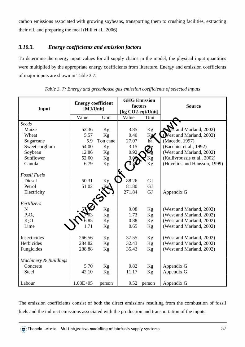
Thapelo Letete - Multiobjective modelling of biofuels supply systems 57
carbon emissions associated with growing soybeans, transporting them to crushing facilities, extracting
their oil, and preparing the meal (Hill et al., 2006).
3.10.3. Energy coefficients and emission factors
To determine the energy input values for all supply chains in the model, the physical input quantities
were multiplied by the appropriate energy coefficients from literature. Energy and emission coefficients
of major inputs are shown in Table 3.7.
Table 3. 7: Energy and greenhouse gas emission coefficients of selected inputs
Energy coefficient [MJ/Unit]
GHG Emission factors
[kg CO2-eqt/Unit] Input
Value Unit Value Unit
Source
Seeds Maize 53.36 Kg 3.85 Kg (West and Marland, 2002) Wheat 5.57 Kg 0.40 Kg (West and Marland, 2002) Sugarcane 5.9 Ton cane 27.07 ha (Macedo, 1997) Sweet sorghum 54.00 Kg 3.15 Kg (Bacchiet et al., 1992) Soybean 12.86 Kg 0.92 Kg (West and Marland, 2002) Sunflower 52.60 Kg 3.06 Kg (Kallivroussis et al., 2002) Canola 6.79 Kg 0.32 Kg (Hovelius and Hansson, 1999) Fossil Fuels Diesel 50.31 Kg 88.26 GJ Petrol 51.02 Kg 81.80 GJ Electricity 271.84 GJ Appendix G Fertilizers N 57.46 Kg 9.08 Kg (West and Marland, 2002) P2O5 7.03 Kg 1.73 Kg (West and Marland, 2002) K2O 6.85 Kg 0.88 Kg (West and Marland, 2002) Lime 1.71 Kg 0.65 Kg (West and Marland, 2002) Insecticides 266.56 Kg 37.55 Kg (West and Marland, 2002) Herbicides 284.82 Kg 32.43 Kg (West and Marland, 2002) Fungicides 288.88 Kg 35.43 Kg (West and Marland, 2002) Machinery & Buildings Concrete 5.70 Kg 0.82 Kg Appendix G Steel 42.10 Kg 11.17 Kg Appendix G Labour 1.08E+05 person 9.52 person Appendix G
The emission coefficients consist of both the direct emissions resulting from the combustion of fossil
fuels and the indirect emissions associated with the production and transportation of the inputs.
Univers
ity of
Cap
e Tow
n
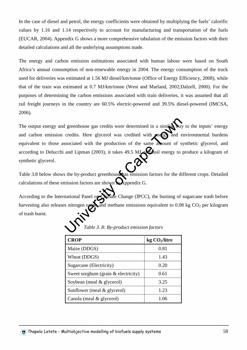
Thapelo Letete - Multiobjective modelling of biofuels supply systems 58
In the case of diesel and petrol, the energy coefficients were obtained by multiplying the fuels’ calorific
values by 1.16 and 1.14 respectively to account for manufacturing and transportation of the fuels
(EUCAR, 2004). Appendix G shows a more comprehensive tabulation of the emission factors with their
detailed calculations and all the underlying assumptions made.
The energy and carbon emission estimations associated with human labour were based on South
Africa’s annual consumption of non-renewable energy in 2004. The energy consumption of the truck
used for deliveries was estimated at 1.56 MJ diesel/km/tonne (Office of Energy Efficiency, 2008), while
that of the train was estimated at 0.7 MJ/km/tonne (West and Marland, 2002;Dalzell, 2000). For the
purposes of determining the carbon emissions associated with train deliveries, it was assumed that all
rail freight journeys in the country are 60.5% electric-powered and 39.5% diesel-powered (IMCSA,
2006).
The output energy and greenhouse gas credits were determined in a similar way to the inputs’ energy
and carbon emission credits. Here glycerol was credited with energy and environmental burdens
equivalent to those associated with the production of the same amount of synthetic glycerol, and
according to Delucchi and Lipman (2003), it takes 49.5 MJ of fossil energy to produce a kilogram of
synthetic glycerol.
Table 3.8 below shows the by-product greenhouse gas emission factors for the different crops. Detailed
calculations of these emission factors are shown in Appendix G.
According to the International Panel on Climate Change (IPCC), the burning of sugarcane trash before
harvesting also releases nitrogen oxide and methane emissions equivalent to 0.08 kg CO2 per kilogram
of trash burnt.
Table 3. 8: By-product emission factors
CROP kg CO2/litre
Maize (DDGS) 0.81
Wheat (DDGS) 1.43
Sugarcane (Electricity) 0.20
Sweet sorghum (grain & electricity) 0.61
Soybean (meal & glycerol) 3.25
Sunflower (meal & glycerol) 1.23
Canola (meal & glycerol) 1.06
Univers
ity of
Cap
e Tow
n
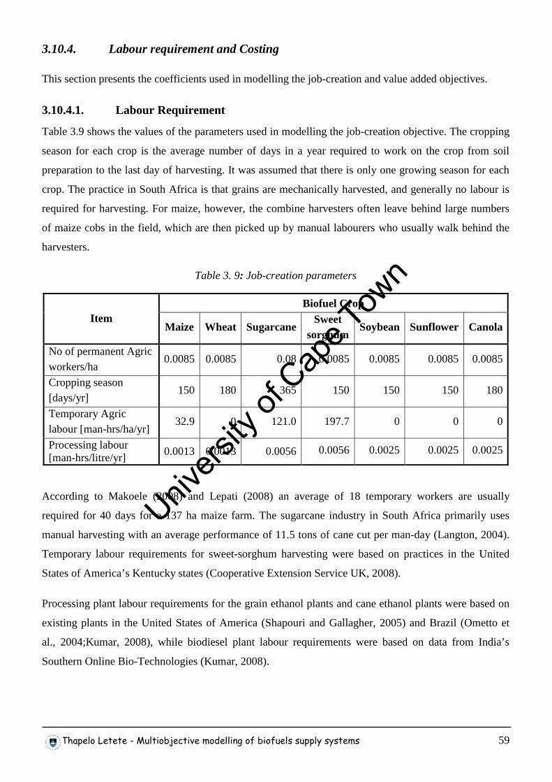
Thapelo Letete - Multiobjective modelling of biofuels supply systems 59
3.10.4. Labour requirement and Costing
This section presents the coefficients used in modelling the job-creation and value added objectives.
3.10.4.1. Labour Requirement
Table 3.9 shows the values of the parameters used in modelling the job-creation objective. The cropping
season for each crop is the average number of days in a year required to work on the crop from soil
preparation to the last day of harvesting. It was assumed that there is only one growing season for each
crop. The practice in South Africa is that grains are mechanically harvested, and generally no labour is
required for harvesting. For maize, however, the combine harvesters often leave behind large numbers
of maize cobs in the field, which are then picked up by manual labourers who usually walk behind the
harvesters.
Table 3. 9: Job-creation parameters
Biofuel Crop Item
Maize Wheat Sugarcane Sweet
sorghum Soybean Sunflower Canola
No of permanent Agric workers/ha
0.0085 0.0085 0.08 0.0085 0.0085 0.0085 0.0085
Cropping season [days/yr]
150 180 365 150 150 150 180
Temporary Agric labour [man-hrs/ha/yr]
32.9 0 121.0 197.7 0 0 0
Processing labour [man-hrs/litre/yr]
0.0013 0.0013 0.0056 0.0056 0.0025 0.0025 0.0025
According to Makoele (2008) and Lepati (2008) an average of 18 temporary workers are usually
required for 40 days for a 137 ha maize farm. The sugarcane industry in South Africa primarily uses
manual harvesting with an average performance of 11.5 tons of cane cut per man-day (Langton, 2004).
Temporary labour requirements for sweet-sorghum harvesting were based on practices in the United
States of America’s Kentucky states (Cooperative Extension Service UK, 2008).
Processing plant labour requirements for the grain ethanol plants and cane ethanol plants were based on
existing plants in the United States of America (Shapouri and Gallagher, 2005) and Brazil (Ometto et
al., 2004;Kumar, 2008), while biodiesel plant labour requirements were based on data from India’s
Southern Online Bio-Technologies (Kumar, 2008).
Univers
ity of
Cap
e Tow
n
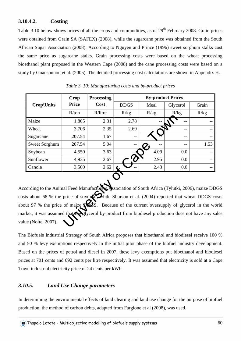
Thapelo Letete - Multiobjective modelling of biofuels supply systems 60
3.10.4.2. Costing
Table 3.10 below shows prices of all the crops and commodities, as of 29th February 2008. Grain prices
were obtained from Grain SA (SAFEX) (2008), while the sugarcane price was obtained from the South
African Sugar Association (2008). According to Nguyen and Prince (1996) sweet sorghum stalks cost
the same price as sugarcane stalks. Grain processing costs were based on the wheat processing
bioethanol plant proposed in the Western Cape (2008) and the cane processing costs were based on a
study by Gnansounou et al. (2005). The detailed processing cost calculations are shown in Appendix H.
Table 3. 10: Manufacturing costs and by-product prices
By-product Prices Crop Price
Processing Cost DDGS Meal Glycerol Grain Crop\Units
R/ton R/litre R/kg R/kg R/kg R/kg
Maize 1,805 2.31 2.78 -- -- --
Wheat 3,706 2.35 2.69 -- -- --
Sugarcane 207.54 1.67 -- -- -- --
Sweet Sorghum 207.54 5.04 -- -- -- 1.53
Soybean 4,550 3.63 -- 4.09 0.0 --
Sunflower 4,935 2.67 -- 2.95 0.0 --
Canola 3,500 2.62 -- 2.43 0.0 --
According to the Animal Feed Manufacturers Association of South Africa (Tylutki, 2006), maize DDGS
costs about 68 % the price of soymeal, while Shurson et al. (2004) reported that wheat DDGS costs
about 97 % the price of maize DDGS. Because of the current oversupply of glycerol in the world
market, it was assumed that the glycerol by-product from biodiesel production does not have any sales
value (Nolte, 2007).
The Biofuels Industrial Strategy of South Africa proposes that bioethanol and biodiesel receive 100 %
and 50 % levy exemptions respectively in the initial pilot phase of the biofuel industry development.
Based on the prices of petrol and diesel in 2007, these levy exemptions put bioethanol and biodiesel
prices at 701 cents and 692 cents per litre respectively. It was assumed that electricity is sold at a Cape
Town industrial electricity price of 24 cents per kWh.
3.10.5. Land Use Change parameters
In determining the environmental effects of land clearing and land use change for the purpose of biofuel
production, the method of carbon debts, adapted from Fargione et al (2008), was used.
Univers
ity of
Cap
e Tow
n
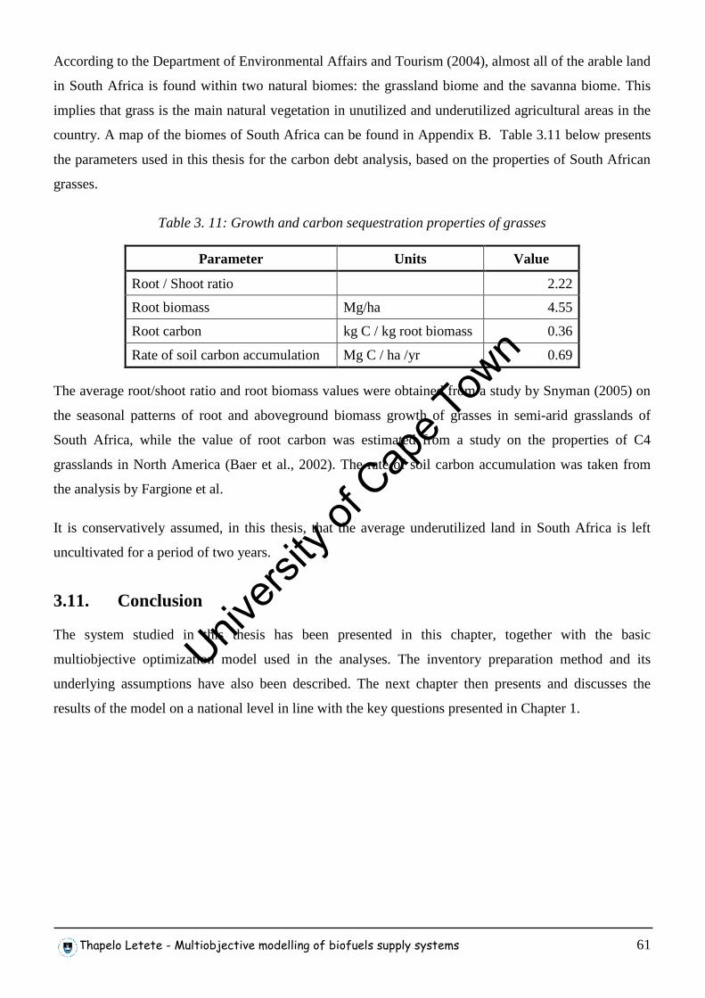
Thapelo Letete - Multiobjective modelling of biofuels supply systems 61
According to the Department of Environmental Affairs and Tourism (2004), almost all of the arable land
in South Africa is found within two natural biomes: the grassland biome and the savanna biome. This
implies that grass is the main natural vegetation in unutilized and underutilized agricultural areas in the
country. A map of the biomes of South Africa can be found in Appendix B. Table 3.11 below presents
the parameters used in this thesis for the carbon debt analysis, based on the properties of South African
grasses.
Table 3. 11: Growth and carbon sequestration properties of grasses
Parameter Units Value
Root / Shoot ratio 2.22
Root biomass Mg/ha 4.55
Root carbon kg C / kg root biomass 0.36
Rate of soil carbon accumulation Mg C / ha /yr 0.69
The average root/shoot ratio and root biomass values were obtained from a study by Snyman (2005) on
the seasonal patterns of root and aboveground biomass growth of grasses in semi-arid grasslands of
South Africa, while the value of root carbon was estimated from a study on the properties of C4
grasslands in North America (Baer et al., 2002). The rate of soil carbon accumulation was taken from
the analysis by Fargione et al.
It is conservatively assumed, in this thesis, that the average underutilized land in South Africa is left
uncultivated for a period of two years.
3.11. Conclusion
The system studied in this thesis has been presented in this chapter, together with the basic
multiobjective optimization model used in the analyses. The inventory preparation method and its
underlying assumptions have also been described. The next chapter then presents and discusses the
results of the model on a national level in line with the key questions presented in Chapter 1.
Univers
ity of
Cap
e Tow
n
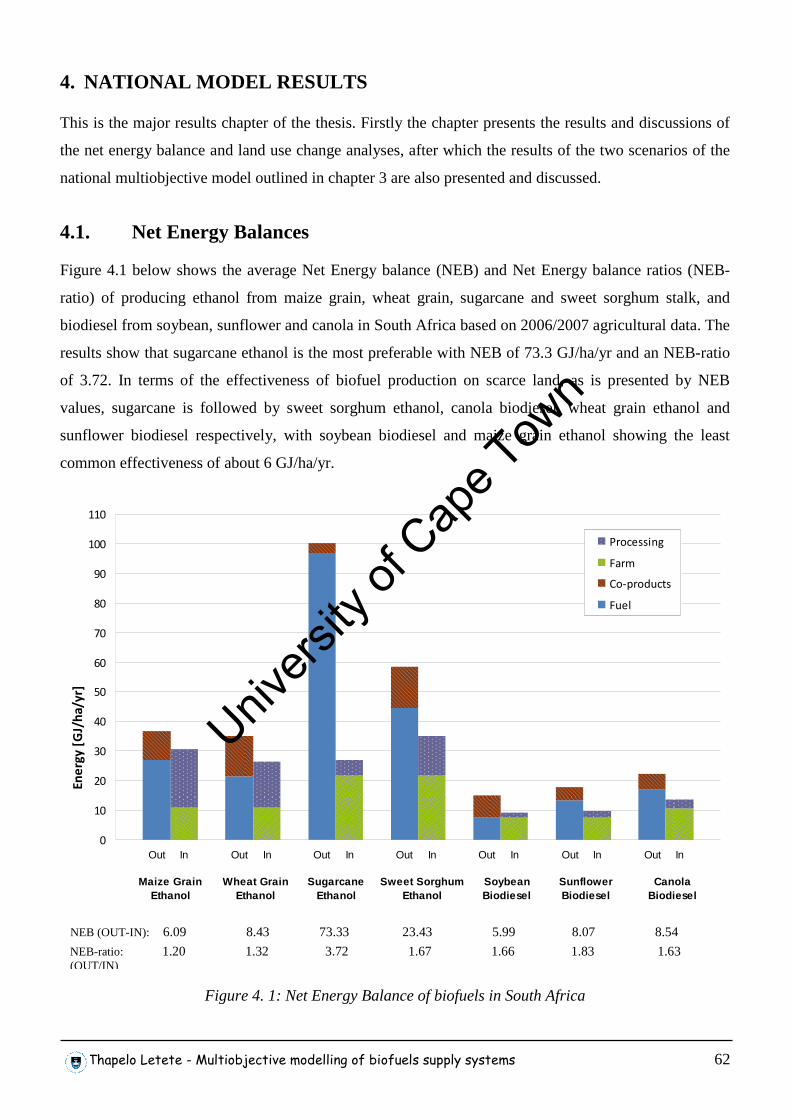
Thapelo Letete - Multiobjective modelling of biofuels supply systems 62
4. NATIONAL MODEL RESULTS
This is the major results chapter of the thesis. Firstly the chapter presents the results and discussions of
the net energy balance and land use change analyses, after which the results of the two scenarios of the
national multiobjective model outlined in chapter 3 are also presented and discussed.
4.1. Net Energy Balances
Figure 4.1 below shows the average Net Energy balance (NEB) and Net Energy balance ratios (NEB-
ratio) of producing ethanol from maize grain, wheat grain, sugarcane and sweet sorghum stalk, and
biodiesel from soybean, sunflower and canola in South Africa based on 2006/2007 agricultural data. The
results show that sugarcane ethanol is the most preferable with NEB of 73.3 GJ/ha/yr and an NEB-ratio
of 3.72. In terms of the effectiveness of biofuel production on scarce land, as is presented by NEB
values, sugarcane is followed by sweet sorghum ethanol, canola biodiesel, wheat grain ethanol and
sunflower biodiesel respectively, with soybean biodiesel and maize grain ethanol showing the least
common effectiveness of about 6 GJ/ha/yr.
0
10
20
30
40
50
60
70
80
90
100
110
Out In Out In Out In Out In Out In Out In Out In
En
erg
y [
GJ/
ha
/yr]
Processing
Farm
Co-products
Fuel
Soybean Biodiesel
Sugarcane Ethanol
Maize Grain Ethanol
Sunflower Biodiesel
Sweet Sorghum Ethanol
Canola Biodiesel
Wheat Grain Ethanol
Figure 4. 1: Net Energy Balance of biofuels in South Africa
NEB (OUT-IN): 6.09 8.43 73.33 23.43 5.99 8.07 8.54
NEB-ratio: 1.20 1.32 3.72 1.67 1.66 1.83 1.63 (OUT/IN)
Univers
ity of
Cap
e Tow
n
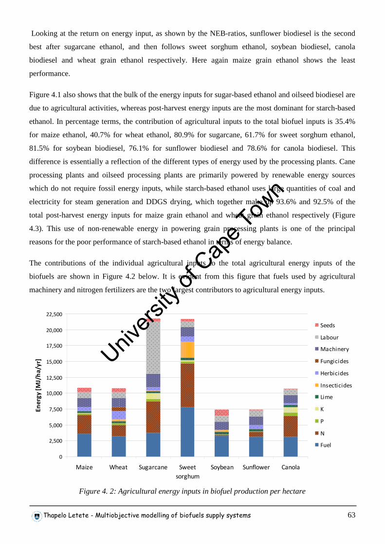
Thapelo Letete - Multiobjective modelling of biofuels supply systems 63
Looking at the return on energy input, as shown by the NEB-ratios, sunflower biodiesel is the second
best after sugarcane ethanol, and then follows sweet sorghum ethanol, soybean biodiesel, canola
biodiesel and wheat grain ethanol respectively. Here again maize grain ethanol shows the least
performance.
Figure 4.1 also shows that the bulk of the energy inputs for sugar-based ethanol and oilseed biodiesel are
due to agricultural activities, whereas post-harvest energy inputs are the most dominant for starch-based
ethanol. In percentage terms, the contribution of agricultural inputs to the total biofuel inputs is 35.4%
for maize ethanol, 40.7% for wheat ethanol, 80.9% for sugarcane, 61.7% for sweet sorghum ethanol,
81.5% for soybean biodiesel, 76.1% for sunflower biodiesel and 78.6% for canola biodiesel. This
difference is essentially a reflection of the different types of energy used by the processing plants. Cane
processing plants and oilseed processing plants are primarily powered by renewable energy sources
which do not require fossil energy inputs, while starch-based ethanol uses large quantities of coal and
electricity for steam generation and DDGS drying, which together make up 93.6% and 92.5% of the
total post-harvest energy inputs for maize grain ethanol and wheat grain ethanol respectively (Figure
4.3). This use of non-renewable energy in powering grain processing plants is one of the principal
reasons for the poor performance of starch-based ethanol in terms of energy balance.
The contributions of the individual agricultural inputs to the total agricultural energy inputs of the
biofuels are shown in Figure 4.2 below. It is evident from this figure that fuels used by agricultural
machinery and nitrogen fertilizers are the two largest contributors to agricultural energy inputs.
0
2,500
5,000
7,500
10,000
12,500
15,000
17,500
20,000
22,500
Maize Wheat Sugarcane Sweet
sorghum
Soybean Sunflower Canola
En
erg
y [
MJ/
ha
/yr]
Seeds
Labour
Machinery
Fungicides
Herbicides
Insecticides
Lime
K
P
N
Fuel
Figure 4. 2: Agricultural energy inputs in biofuel production per hectare
Univers
ity of
Cap
e Tow
n
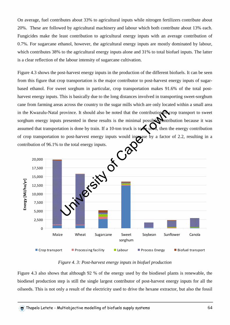
Thapelo Letete - Multiobjective modelling of biofuels supply systems 64
On average, fuel contributes about 33% to agricultural inputs while nitrogen fertilizers contribute about
20%. These are followed by agricultural machinery and labour which both contribute about 13% each.
Fungicides make the least contribution to agricultural energy inputs with an average contribution of
0.7%. For sugarcane ethanol, however, the agricultural energy inputs are mostly dominated by labour,
which contributes 38% to the agricultural energy inputs alone and 31% to total biofuel inputs. The latter
is a clear reflection of the labour intensity of sugarcane cultivation.
Figure 4.3 shows the post-harvest energy inputs in the production of the different biofuels. It can be seen
from this figure that crop transportation is the major contributor to post-harvest energy inputs of sugar-
based ethanol. For sweet sorghum in particular, crop transportation makes 91.6% of the total post-
harvest energy inputs. This is basically due to the long distances involved in transporting sweet-sorghum
cane from farming areas across the country to the sugar mills which are only located within a small area
in the Kwazulu-Natal province. It should also be noted that the contribution of crop transport to sweet
sorghum energy inputs presented in these results is the minimal possible contribution because it was
assumed that transportation is done by train. If a 10-ton truck is to be used, then the energy contribution
of crop transportation to post-harvest energy inputs would increase by a factor of 2.2, resulting in a
contribution of 96.1% to the total energy inputs.
0
2,500
5,000
7,500
10,000
12,500
15,000
17,500
20,000
Maize Wheat Sugarcane Sweet
sorghum
Soybean Sunflower Canola
En
erg
y [
MJ/
ha
/yr]
Crop transport Processing facil ity Labour Process Energy Biofuel transport
Figure 4. 3: Post-harvest energy inputs in biofuel production
Figure 4.3 also shows that although 92 % of the energy used by the biodiesel plants is renewable, the
biodiesel production step is still the single largest contributor of post-harvest energy inputs for all the
oilseeds. This is not only a result of the electricity used to drive the hexane extractor, but also the fossil
Univers
ity of
Cap
e Tow
n
Thapelo Letete - Multiobjective modelling of biofuels supply systems 65
energy required to manufacture and transport the reagents and solvents used in the transesterification
process. On its own, the latter contributes to 49%, 63% and 64% of post-harvest energy inputs for
soybean biodiesel, sunflower biodiesel and canola biodiesel.
The individual NEB-ratio values for each biofuel are discussed in the following sections:
4.1.1. Maize Grain Ethanol
The difference between the NEB-ratio of 1.20 shown in Figure 4.1 above and that calculated by Ethanol
Africa themselves (1.63) is primarily due to the different system boundaries considered in the two cases.
While all life-cycle energy inputs of maize grain ethanol from farming to the blending station have been
considered in this thesis, Ethanol Africa have only included farm fossil fuel use, crop transportation and
processing plant energy use in their analysis; accounting for only 75 % of the energy inputs into the
production of maize grain ethanol. The same is true for the National Biofuels Study (2006) which
reports an energy balance ratio of 1.36. If only 75% of the energy inputs are analysed in this thesis, the
NEB-ratio becomes 1.56. It should be noted, however, that with both the Ethanol Africa and the
National Biofuels Study it is not clear how co-product energy allocation was carried out.
4.1.2. Wheat Grain Ethanol
No studies were found on the net energy balance of wheat grain ethanol production in South Africa.
Instead two studies based on the production of wheat grain ethanol in Europe were used for comparison;
studies by Richards (2000) and Elsayed et al. (2003) which present NEB-ratios of 1.1 and 2.16
respectively. Apart from the fact that the European agricultural inputs and yields are very different from
those in South Africa, there are also a number of analytical differences between this thesis and these
studies that have led to the different NEB-ratios: While both of these studies exclude the fossil energy
inputs associated with labour and the manufacture of agricultural machinery, the study by Richards
further excludes energy inputs associated with construction of the processing plant and biofuel
distribution. This amounts to 9.5% and 9.1% of energy inputs excluded in the analyses by Richards and
Elsayed et al. respectively. With regards to allocation, the study by Richards does not mention any
allocation, although the analysis simply excludes energy credits for DDGS. In the study by Elsayed et al.
allocation of co-product energy credits is based on market prices and not product substitution, and also it
is assumed that wheat straw has a market value hence not ploughed back into the field.
4.1.3. Sugarcane Ethanol
The National Biofuels Study (2006) reports an NEB-ratio of 6.02 for South African fuel bio-ethanol
made from sugarcane. Similar to the previous cases, the difference between this value and that of 3.72
Univers
ity of
Cap
e Tow
n
Thapelo Letete - Multiobjective modelling of biofuels supply systems 66
reported in Figure 4.1 is mainly due to the difference in the energy inputs included in these analyses.
The National Biofuels study leaves out the energy inputs associated with labour, seed production,
production of agricultural machinery and facility construction, all of which amount to 45 % of energy
inputs that are not accounted for. If the contributions of energy inputs associated with labour, seed
production, agricultural machinery production and process facility construction are excluded in this
thesis, then the NEB-ratio also increases to 6.81; a value which differs from that reported by the
National Biofuels Study by only 13%.
4.1.4. Sweet Sorghum Ethanol
Grassi (2001) estimated the NEB-ratio of sweet sorghum ethanol production in Brazil and sub-Saharan
Africa at 6.5. Unfortunately the calculations and allocation procedures are not clearly given in that
study, making it impossible to conduct a detailed comparison. It was observed, however, that the system
boundary definition in the study by Grassi is much narrower than that adopted in this thesis; in
particular, the energy inputs associated with production of agricultural machinery, construction of
processing facilities and labour have not been included in that analysis. In total, about 8.5% of the fossil
energy inputs considered here seem to have been excluded in the study by Grassi. Overall, it was noted
that the reason for the poor NEB-ratio in this thesis is the excessive distances assumed for transporting
the sorghum cane from the farm to the processing plants.
4.1.5. Soybean Biodiesel
The difference between the soybean biodiesel NEB-ratio of 1.66 shown in Figure 4.1 and that of 3.22
calculated by Sheehan et al (1998) for the US Midwest case is a result of two major factors; the different
energy inputs considered in the two studies and the different allocation methods adopted in these studies.
In the study by Sheehan et al., the energy associated with farm machinery, labour and construction of
processing facilities have all been excluded in the energy balance, making up 26% of fossil energy
inputs. Sheehan et al. also use mass allocation to assign co-product energy flows instead of product
substitution. That notwithstanding, it appears that there is a tangible geographical difference between
soybean biodiesel production in the US Midwest and in South Africa, with agricultural practices and
yields giving the former an advantage.
The National Biofuels Study (2006) on the other hand reports a net energy balance of 2.40 for biodiesel
production in South Africa. As with the study by Sheehan et al., only energy flows contributing to 74 %
of the energy inputs have been accounted for in the National Biofuels Study, except that in the latter it is
not clear which allocation method was used. If only 74% of the fossil energy inputs to soybean biodiesel
Univers
ity of
Cap
e Tow
n
Thapelo Letete - Multiobjective modelling of biofuels supply systems 67
production are accounted for in this thesis, the NEB-ratio becomes 2.24, which is 93% of that calculated
by the National Biofuels Study.
4.1.6. Sunflower Biodiesel
Studies on the net energy balance of sunflower biodiesel based on South African data were not found,
hence a study by Kallivroussis et al. (2002) based on sunflower production in Greece was used for
comparison. While Figure 4.1 reports NEB-ratio of 1.83, the study by Kallivroussis et al. reports a net
energy balance ratio of 4.5. Apart from the agricultural inputs and yields which are different from those
in South Africa, the difference between this value and the one obtained in Figure 4.1 above is a result of
two major factors: The difference in system boundaries of the two studies and the different allocation
methods adopted. The study by Kallivroussis et al. (2002) only presents an energy balance around the
agricultural production of sunflower oil, and do not include the conversion of sunflower oil into
biodiesel, thus leaving out a total of 41 % of the fossil energy inputs into the production of sunflower
biodiesel. Also in the analysis by Kallivroussis et al., the cake was credited with the energy equivalent to
its calorific value (19.6 MJ/kg); a value which is 5 times larger than the value it would be credited with
if product substitution was used.
4.1.7. Canola Biodiesel
There have not been any studies on the net energy balance of biodiesel production from canola in South
Africa; hence studies based on the production of biodiesel from rapeseed in Europe were used for
comparison. Richards (2000) reports a NEB-ratio value of 1.82 while Elsayed et al. report a NEB-value
of 2.29. As pointed out in section 4.1.2., both of these studies exclude some energy inputs which are
analysed in this thesis. For the production of canola biodiesel, the total percentage of energy inputs that
have not been included in these two studies is 18.8% in the analysis by Richards and 17.6% in the
analysis by Elsayed et al. The study by Richards also excludes glycerol energy credits.
4.1.8. Conclusions
Despite the use of expansive system boundaries for energy inputs in this analysis, it can be concluded
that the South African production of maize grain ethanol, wheat grain ethanol, sugarcane ethanol, sweet
sorghum ethanol, soybean biodiesel, sunflower biodiesel and canola biodiesel all result in net energy
gains. From an energy balance perspective only, sugarcane is by far the best option for ethanol
production in South Africa, while maize is the least preferable.
Univers
ity of
Cap
e Tow
n
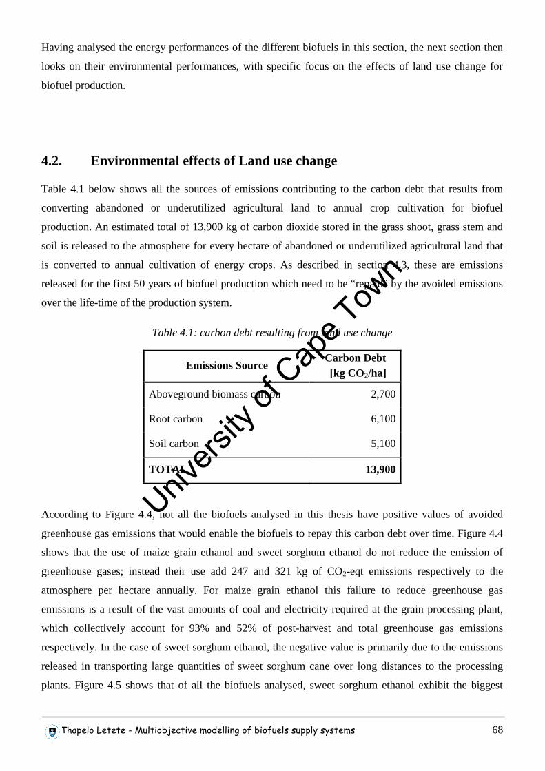
Thapelo Letete - Multiobjective modelling of biofuels supply systems 68
Having analysed the energy performances of the different biofuels in this section, the next section then
looks on their environmental performances, with specific focus on the effects of land use change for
biofuel production.
4.2. Environmental effects of Land use change
Table 4.1 below shows all the sources of emissions contributing to the carbon debt that results from
converting abandoned or underutilized agricultural land to annual crop cultivation for biofuel
production. An estimated total of 13,900 kg of carbon dioxide stored in the grass shoot, grass stem and
soil is released to the atmosphere for every hectare of abandoned or underutilized agricultural land that
is converted to annual cultivation of energy crops. As described in section 4.3, these are emissions
released for the first 50 years of biofuel production which need to be “repaid” by the avoided emissions
over the life-time of the production system.
Table 4.1: carbon debt resulting from land use change
Emissions Source Carbon Debt [kg CO2/ha]
Aboveground biomass carbon 2,700
Root carbon 6,100
Soil carbon 5,100
TOTAL 13,900
According to Figure 4.4, not all the biofuels analysed in this thesis have positive values of avoided
greenhouse gas emissions that would enable the biofuels to repay this carbon debt over time. Figure 4.4
shows that the use of maize grain ethanol and sweet sorghum ethanol do not reduce the emission of
greenhouse gases; instead their use add 247 and 321 kg of CO2-eqt emissions respectively to the
atmosphere per hectare annually. For maize grain ethanol this failure to reduce greenhouse gas
emissions is a result of the vast amounts of coal and electricity required at the grain processing plant,
which collectively account for 93% and 52% of post-harvest and total greenhouse gas emissions
respectively. In the case of sweet sorghum ethanol, the negative value is primarily due to the emissions
released in transporting large quantities of sweet sorghum cane over long distances to the processing
plants. Figure 4.5 shows that of all the biofuels analysed, sweet sorghum ethanol exhibit the biggest
Univers
ity of
Cap
e Tow
n
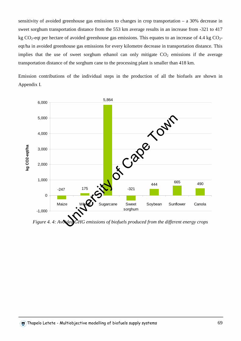
Thapelo Letete - Multiobjective modelling of biofuels supply systems 69
sensitivity of avoided greenhouse gas emissions to changes in crop transportation – a 30% decrease in
sweet sorghum transportation distance from the 553 km average results in an increase from -321 to 417
kg CO2-eqt per hectare of avoided greenhouse gas emissions. This equates to an increase of 4.4 kg CO2-
eqt/ha in avoided greenhouse gas emissions for every kilometre decrease in transportation distance. This
implies that the use of sweet sorghum ethanol can only mitigate CO2 emissions if the average
transportation distance of the sorghum cane to the processing plant is smaller than 418 km.
Emission contributions of the individual steps in the production of all the biofuels are shown in
Appendix I.
175444 490665
5,864
-321-247
-1,000
0
1,000
2,000
3,000
4,000
5,000
6,000
Maize Wheat Sugarcane Sweetsorghum
Soybean Sunflower Canola
kg C
O2-
eqt/h
a
Figure 4. 4: Avoided GHG emissions of biofuels produced from the different energy crops Univ
ersity
of C
ape T
own
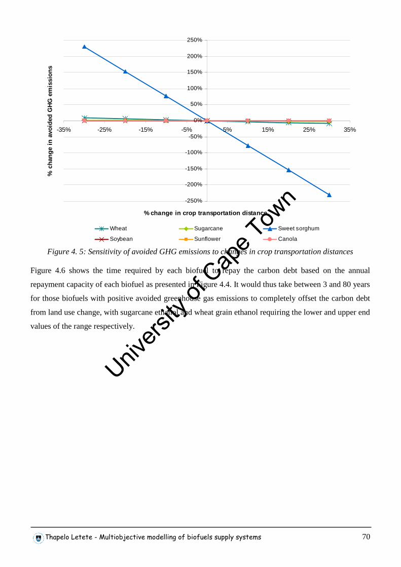
Thapelo Letete - Multiobjective modelling of biofuels supply systems 70
-250%
-200%
-150%
-100%
-50%
0%
50%
100%
150%
200%
250%
-35% -25% -15% -5% 5% 15% 25% 35%
% change in crop transportation distance
% c
hang
e in
avo
ided
GH
G e
mis
sion
s
Wheat Sugarcane Sweet sorghum
Soybean Sunflower Canola
Figure 4. 5: Sensitivity of avoided GHG emissions to changes in crop transportation distances
Figure 4.6 shows the time required by each biofuel to repay the carbon debt based on the annual
repayment capacity of each biofuel as presented in Figure 4.4. It would thus take between 3 and 80 years
for those biofuels with positive avoided greenhouse gas emissions to completely offset the carbon debt
from land use change, with sugarcane ethanol and wheat grain ethanol requiring the lower and upper end
values of the range respectively.
Univers
ity of
Cap
e Tow
n
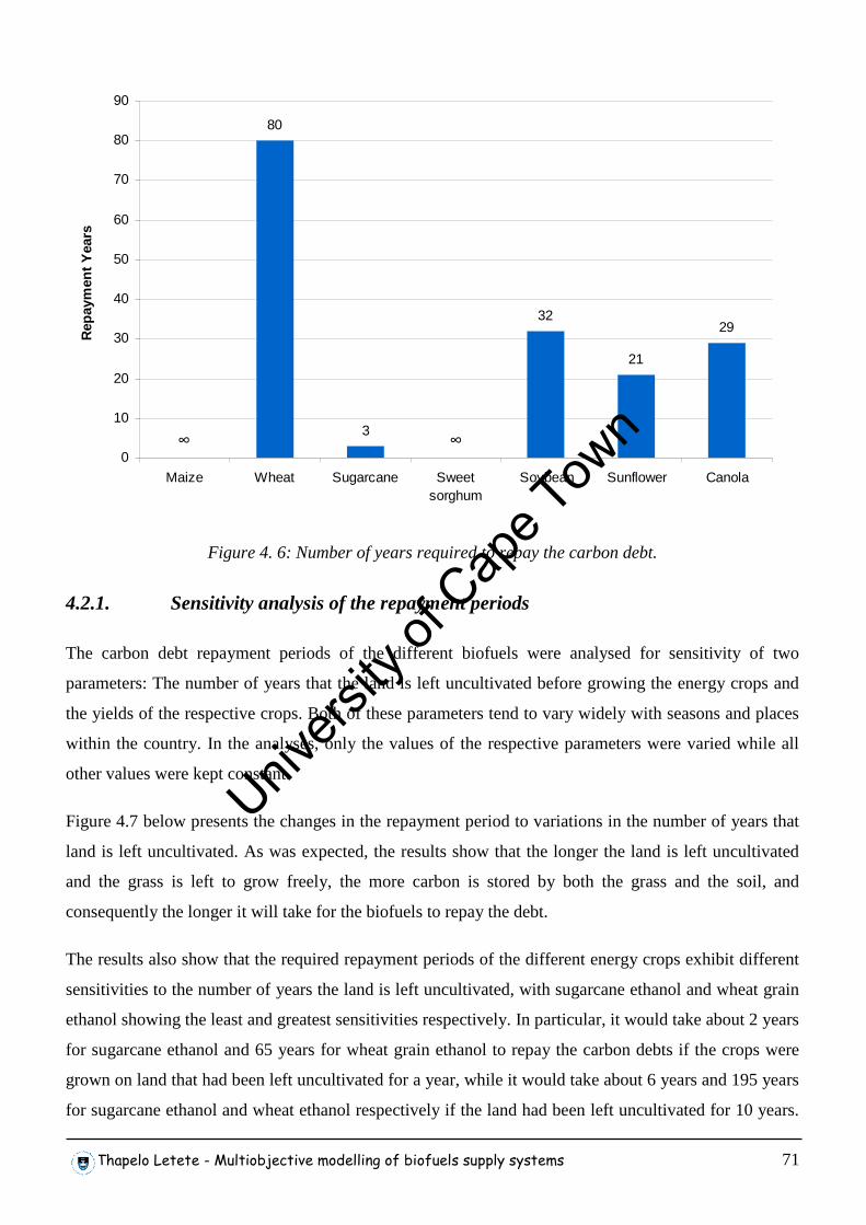
Thapelo Letete - Multiobjective modelling of biofuels supply systems 71
80
3
32
21
29
∞ ∞
0
10
20
30
40
50
60
70
80
90
Maize Wheat Sugarcane Sweetsorghum
Soybean Sunflower Canola
Rep
aym
ent Y
ears
Figure 4. 6: Number of years required to repay the carbon debt.
4.2.1. Sensitivity analysis of the repayment periods
The carbon debt repayment periods of the different biofuels were analysed for sensitivity of two
parameters: The number of years that the land is left uncultivated before growing the energy crops and
the yields of the respective crops. Both of these parameters tend to vary widely with seasons and places
within the country. In the analyses, only the values of the respective parameters were varied while all
other values were kept constant.
Figure 4.7 below presents the changes in the repayment period to variations in the number of years that
land is left uncultivated. As was expected, the results show that the longer the land is left uncultivated
and the grass is left to grow freely, the more carbon is stored by both the grass and the soil, and
consequently the longer it will take for the biofuels to repay the debt.
The results also show that the required repayment periods of the different energy crops exhibit different
sensitivities to the number of years the land is left uncultivated, with sugarcane ethanol and wheat grain
ethanol showing the least and greatest sensitivities respectively. In particular, it would take about 2 years
for sugarcane ethanol and 65 years for wheat grain ethanol to repay the carbon debts if the crops were
grown on land that had been left uncultivated for a year, while it would take about 6 years and 195 years
for sugarcane ethanol and wheat ethanol respectively if the land had been left uncultivated for 10 years.
Univers
ity of
Cap
e Tow
n
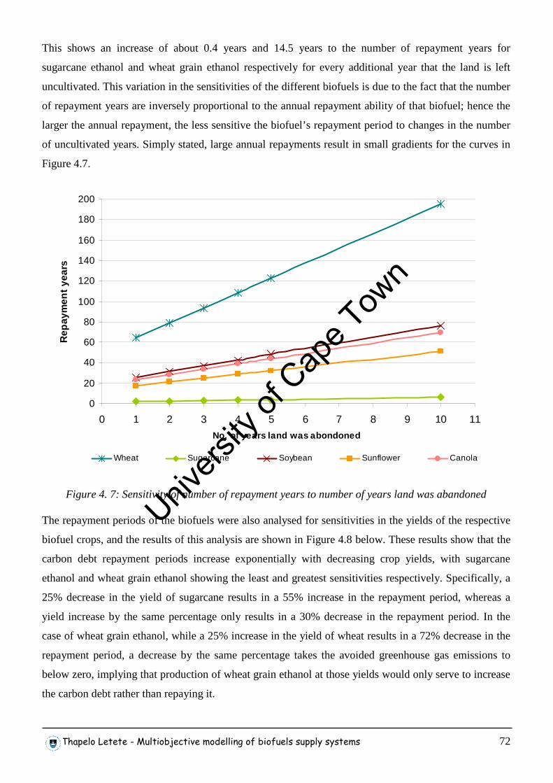
Thapelo Letete - Multiobjective modelling of biofuels supply systems 72
This shows an increase of about 0.4 years and 14.5 years to the number of repayment years for
sugarcane ethanol and wheat grain ethanol respectively for every additional year that the land is left
uncultivated. This variation in the sensitivities of the different biofuels is due to the fact that the number
of repayment years are inversely proportional to the annual repayment ability of that biofuel; hence the
larger the annual repayment, the less sensitive the biofuel’s repayment period to changes in the number
of uncultivated years. Simply stated, large annual repayments result in small gradients for the curves in
Figure 4.7.
0
20
40
60
80
100
120
140
160
180
200
0 1 2 3 4 5 6 7 8 9 10 11
No. of years land was abondoned
Rep
aym
ent y
ears
Wheat Sugarcane Soybean Sunflower Canola
Figure 4. 7: Sensitivity of number of repayment years to number of years land was abandoned
The repayment periods of the biofuels were also analysed for sensitivities in the yields of the respective
biofuel crops, and the results of this analysis are shown in Figure 4.8 below. These results show that the
carbon debt repayment periods increase exponentially with decreasing crop yields, with sugarcane
ethanol and wheat grain ethanol showing the least and greatest sensitivities respectively. Specifically, a
25% decrease in the yield of sugarcane results in a 55% increase in the repayment period, whereas a
yield increase by the same percentage only results in a 30% decrease in the repayment period. In the
case of wheat grain ethanol, while a 25% increase in the yield of wheat results in a 72% decrease in the
repayment period, a decrease by the same percentage takes the avoided greenhouse gas emissions to
below zero, implying that production of wheat grain ethanol at those yields would only serve to increase
the carbon debt rather than repaying it.
Univers
ity of
Cap
e Tow
n
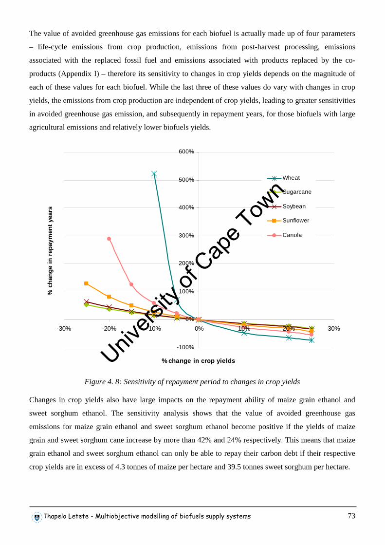
Thapelo Letete - Multiobjective modelling of biofuels supply systems 73
The value of avoided greenhouse gas emissions for each biofuel is actually made up of four parameters
– life-cycle emissions from crop production, emissions from post-harvest processing, emissions
associated with the replaced fossil fuel and emissions associated with products replaced by the co-
products (Appendix I) – therefore its sensitivity to changes in crop yields depends on the magnitude of
each of these values for each biofuel. While the last three of these values do vary with changes in crop
yields, the emissions from crop production are independent of crop yields, leading to greater sensitivities
in avoided greenhouse gas emission, and subsequently in repayment years, for those biofuels with large
agricultural emissions and relatively lower biofuels yields.
-100%
0%
100%
200%
300%
400%
500%
600%
-30% -20% -10% 0% 10% 20% 30%
% change in crop yields
% c
hang
e in
rep
aym
ent y
ears
Wheat
Sugarcane
Soybean
Sunflower
Canola
Figure 4. 8: Sensitivity of repayment period to changes in crop yields
Changes in crop yields also have large impacts on the repayment ability of maize grain ethanol and
sweet sorghum ethanol. The sensitivity analysis shows that the value of avoided greenhouse gas
emissions for maize grain ethanol and sweet sorghum ethanol become positive if the yields of maize
grain and sweet sorghum cane increase by more than 42% and 24% respectively. This means that maize
grain ethanol and sweet sorghum ethanol can only be able to repay their carbon debt if their respective
crop yields are in excess of 4.3 tonnes of maize per hectare and 39.5 tonnes sweet sorghum per hectare.
Univers
ity of
Cap
e Tow
n
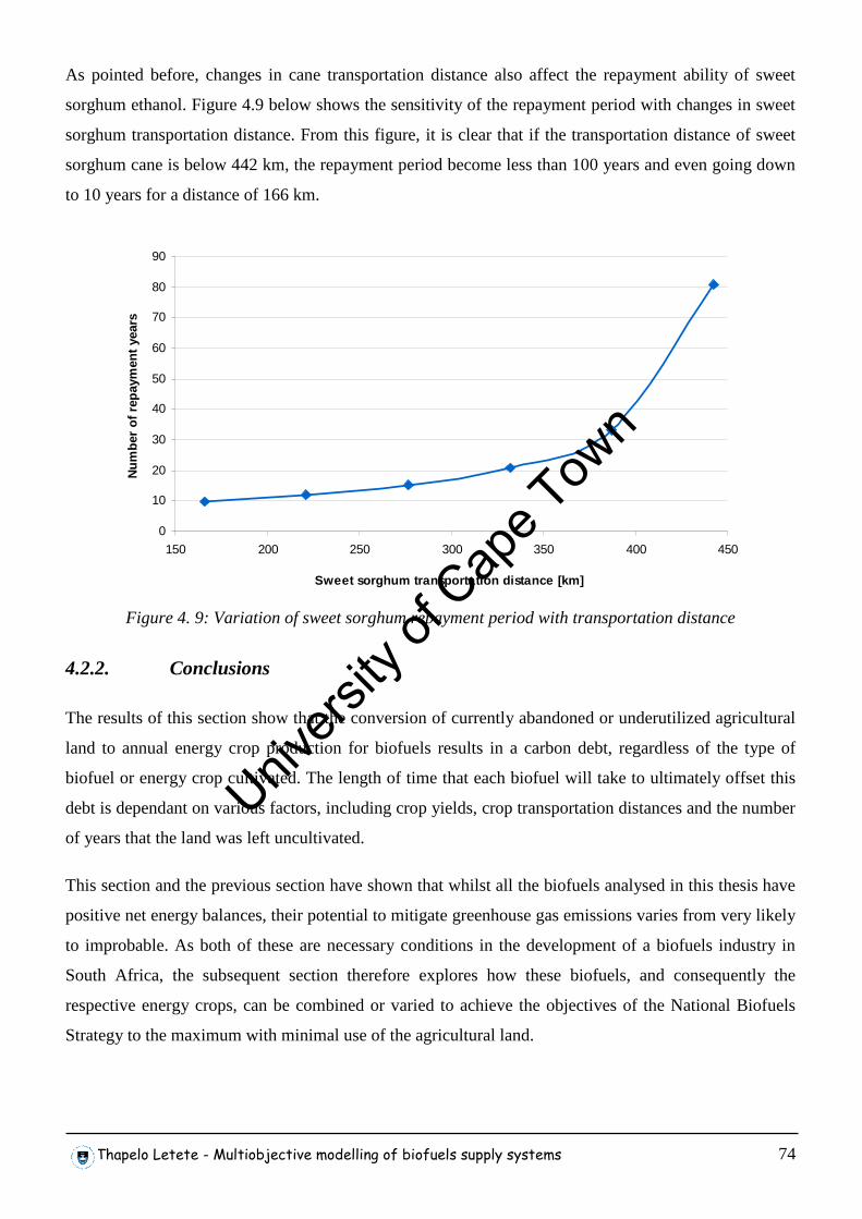
Thapelo Letete - Multiobjective modelling of biofuels supply systems 74
As pointed before, changes in cane transportation distance also affect the repayment ability of sweet
sorghum ethanol. Figure 4.9 below shows the sensitivity of the repayment period with changes in sweet
sorghum transportation distance. From this figure, it is clear that if the transportation distance of sweet
sorghum cane is below 442 km, the repayment period become less than 100 years and even going down
to 10 years for a distance of 166 km.
0
10
20
30
40
50
60
70
80
90
150 200 250 300 350 400 450
Sweet sorghum transportation distance [km]
Num
ber
of r
epay
men
t yea
rs
Figure 4. 9: Variation of sweet sorghum repayment period with transportation distance
4.2.2. Conclusions
The results of this section show that the conversion of currently abandoned or underutilized agricultural
land to annual energy crop production for biofuels results in a carbon debt, regardless of the type of
biofuel or energy crop cultivated. The length of time that each biofuel will take to ultimately offset this
debt is dependant on various factors, including crop yields, crop transportation distances and the number
of years that the land was left uncultivated.
This section and the previous section have shown that whilst all the biofuels analysed in this thesis have
positive net energy balances, their potential to mitigate greenhouse gas emissions varies from very likely
to improbable. As both of these are necessary conditions in the development of a biofuels industry in
South Africa, the subsequent section therefore explores how these biofuels, and consequently the
respective energy crops, can be combined or varied to achieve the objectives of the National Biofuels
Strategy to the maximum with minimal use of the agricultural land.
Univers
ity of
Cap
e Tow
n
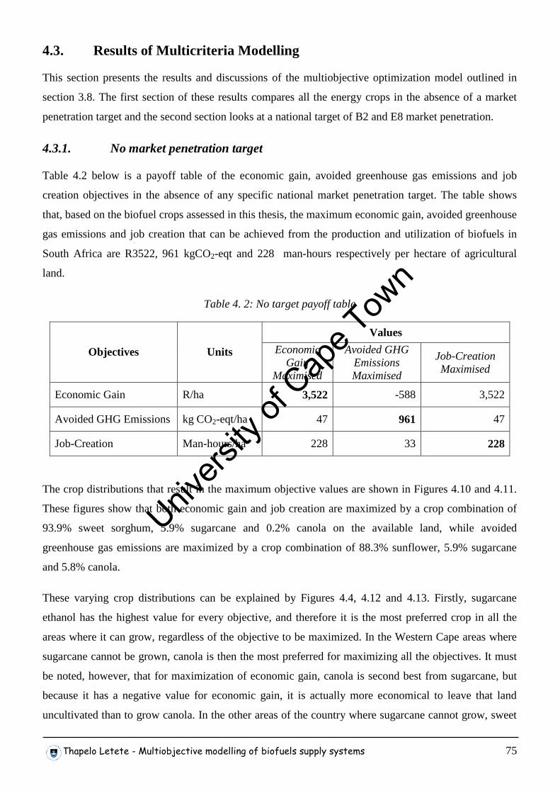
Thapelo Letete - Multiobjective modelling of biofuels supply systems 75
4.3. Results of Multicriteria Modelling
This section presents the results and discussions of the multiobjective optimization model outlined in
section 3.8. The first section of these results compares all the energy crops in the absence of a market
penetration target and the second section looks at a national target of B2 and E8 market penetration.
4.3.1. No market penetration target
Table 4.2 below is a payoff table of the economic gain, avoided greenhouse gas emissions and job
creation objectives in the absence of any specific national market penetration target. The table shows
that, based on the biofuel crops assessed in this thesis, the maximum economic gain, avoided greenhouse
gas emissions and job creation that can be achieved from the production and utilization of biofuels in
South Africa are R3522, 961 kgCO2-eqt and 228 man-hours respectively per hectare of agricultural
land.
Table 4. 2: No target payoff table
Values
Objectives Units Economic Gain
Maximised
Avoided GHG Emissions Maximised
Job-Creation Maximised
Economic Gain R/ha 3,522 -588 3,522
Avoided GHG Emissions kg CO2-eqt/ha 47 961 47
Job-Creation Man-hours/ha 228 33 228
The crop distributions that result in the maximum objective values are shown in Figures 4.10 and 4.11.
These figures show that both economic gain and job creation are maximized by a crop combination of
93.9% sweet sorghum, 5.9% sugarcane and 0.2% canola on the available land, while avoided
greenhouse gas emissions are maximized by a crop combination of 88.3% sunflower, 5.9% sugarcane
and 5.8% canola.
These varying crop distributions can be explained by Figures 4.4, 4.12 and 4.13. Firstly, sugarcane
ethanol has the highest value for every objective, and therefore it is the most preferred crop in all the
areas where it can grow, regardless of the objective to be maximized. In the Western Cape areas where
sugarcane cannot be grown, canola is then the most preferred for maximizing all the objectives. It must
be noted, however, that for maximization of economic gain, canola is second best from sugarcane, but
because it has a negative value for economic gain, it is actually more economical to leave that land
uncultivated than to grow canola. In the other areas of the country where sugarcane cannot grow, sweet
Univers
ity of
Cap
e Tow
n
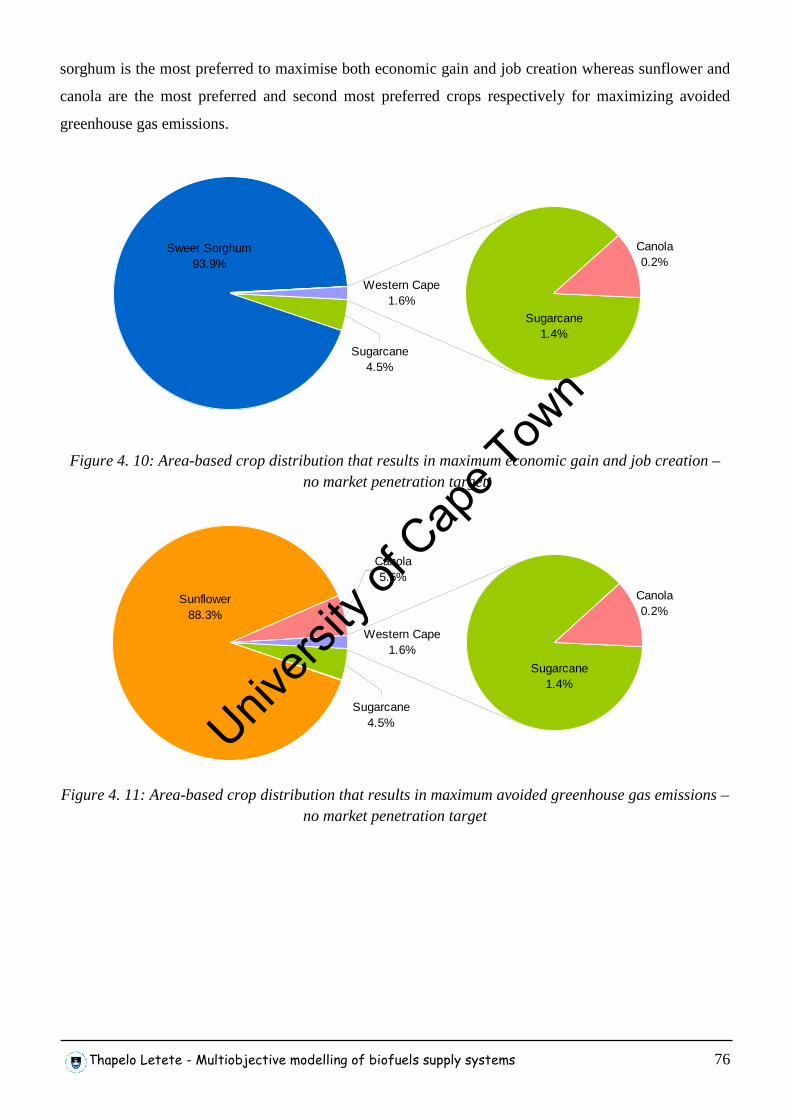
Thapelo Letete - Multiobjective modelling of biofuels supply systems 76
sorghum is the most preferred to maximise both economic gain and job creation whereas sunflower and
canola are the most preferred and second most preferred crops respectively for maximizing avoided
greenhouse gas emissions.
Sugarcane1.4%
Sugarcane4.5%
Sweet Sorghum93.9%
Canola0.2%
Western Cape1.6%
Figure 4. 10: Area-based crop distribution that results in maximum economic gain and job creation – no market penetration target
Western Cape1.6%
Canola0.2%
Sugarcane4.5%
Canola5.6%
Sunflower88.3%
Sugarcane1.4%
Figure 4. 11: Area-based crop distribution that results in maximum avoided greenhouse gas emissions –
no market penetration target
Univers
ity of
Cap
e Tow
n
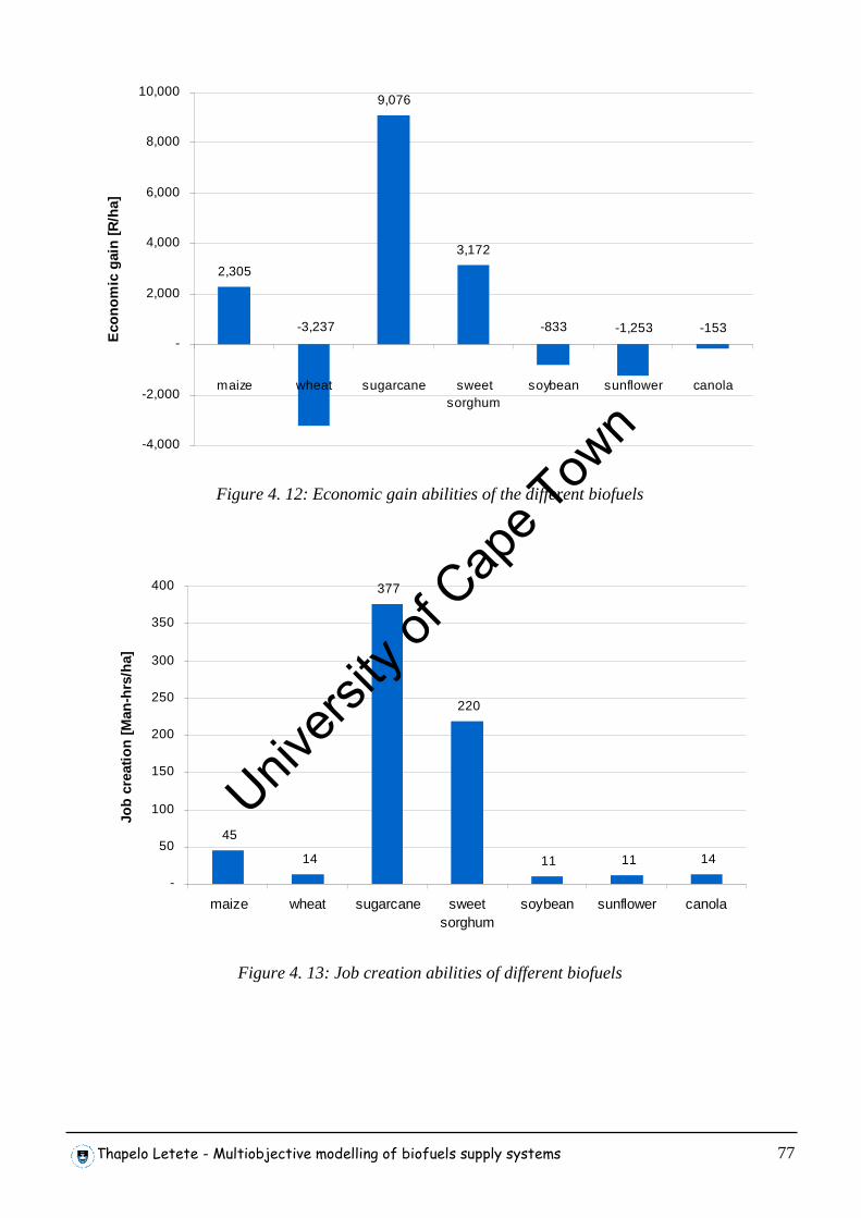
Thapelo Letete - Multiobjective modelling of biofuels supply systems 77
2,305
9,076
3,172
-153 -1,253 -833 -3,237
-4,000
-2,000
-
2,000
4,000
6,000
8,000
10,000
maize wheat sugarcane sweetsorghum
soybean sunflower canola
Eco
nom
ic g
ain
[R/h
a]
Figure 4. 12: Economic gain abilities of the different biofuels
45
14
377
220
11 11 14
-
50
100
150
200
250
300
350
400
maize wheat sugarcane sweetsorghum
soybean sunflower canola
Job
crea
tion
[Man
-hrs
/ha]
Figure 4. 13: Job creation abilities of different biofuels
Univers
ity of
Cap
e Tow
n
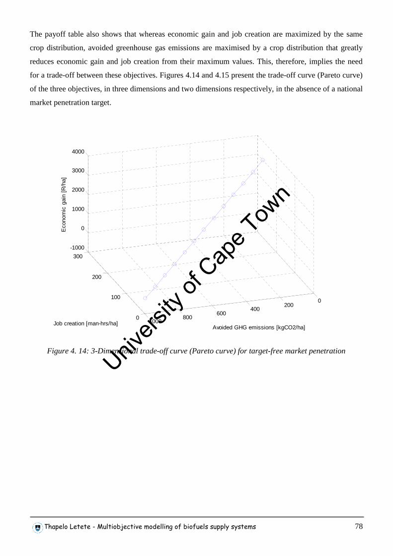
Thapelo Letete - Multiobjective modelling of biofuels supply systems 78
The payoff table also shows that whereas economic gain and job creation are maximized by the same
crop distribution, avoided greenhouse gas emissions are maximised by a crop distribution that greatly
reduces economic gain and job creation from their maximum values. This, therefore, implies the need
for a trade-off between these objectives. Figures 4.14 and 4.15 present the trade-off curve (Pareto curve)
of the three objectives, in three dimensions and two dimensions respectively, in the absence of a national
market penetration target.
0
100
200
300
0200
400600
8001000
-1000
0
1000
2000
3000
4000
Avoided GHG emissions [kgCO2/ha]Job creation [man-hrs/ha]
Eco
nom
ic g
ain
[R/h
a]
Figure 4. 14: 3-Dimensional trade-off curve (Pareto curve) for target-free market penetration
Univers
ity of
Cap
e Tow
n
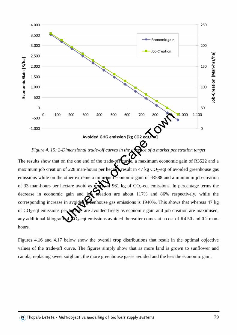
Thapelo Letete - Multiobjective modelling of biofuels supply systems 79
-1,000
-500
0
500
1,000
1,500
2,000
2,500
3,000
3,500
4,000
0 100 200 300 400 500 600 700 800 900 1,000 1,100
Avoided GHG emission [kg CO2 eqt/ha]
Eco
no
mic
Ga
in [
R/h
a]
0
50
100
150
200
250
Job
-Cre
ati
on
[M
an
-hrs
/ha
]
Economic gain
Job-Creation
Figure 4. 15: 2-Dimensional trade-off curves in the absence of a market penetration target
The results show that on the one end of the trade-off curve, a maximum economic gain of R3522 and a
maximum job creation of 228 man-hours per hectare result in 47 kg CO2-eqt of avoided greenhouse gas
emissions while on the other extreme a minimum economic gain of -R588 and a minimum job-creation
of 33 man-hours per hectare avoid as much as 961 kg of CO2-eqt emissions. In percentage terms the
decrease in economic gain and job creation are about 117% and 86% respectively, while the
corresponding increase in avoided greenhouse gas emissions is 1940%. This shows that whereas 47 kg
of CO2-eqt emissions per hectare are avoided freely as economic gain and job creation are maximised,
any additional kilogram of CO2-eqt emissions avoided thereafter comes at a cost of R4.50 and 0.2 man-
hours.
Figures 4.16 and 4.17 below show the overall crop distributions that result in the optimal objective
values of the trade-off curve. The figures simply show that as more land is grown to sunflower and
canola, replacing sweet sorghum, the more greenhouse gases avoided and the less the economic gain.
Univers
ity of
Cap
e Tow
n
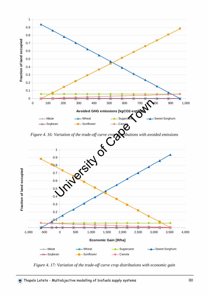
Thapelo Letete - Multiobjective modelling of biofuels supply systems 80
0
0.1
0.2
0.3
0.4
0.5
0.6
0.7
0.8
0.9
1
0 100 200 300 400 500 600 700 800 900 1,000
Avoided GHG emissions [kgCO2-eqt/ha]
Fra
ctio
n of
land
occ
upie
d
Maize Wheat Sugarcane Sweet Sorghum
Soybean Sunflower Canola
Figure 4. 16: Variation of the trade-off curve crop distributions with avoided emissions
0
0.1
0.2
0.3
0.4
0.5
0.6
0.7
0.8
0.9
1
-1,000 -500 0 500 1,000 1,500 2,000 2,500 3,000 3,500 4,000
Economic Gain [R/ha]
Fra
ctio
n of
land
occ
upie
d
Maize Wheat Sugarcane Sweet Sorghum
Soybean Sunflower Canola
Figure 4. 17: Variation of the trade-off curve crop distributions with economic gain
Univers
ity of
Cap
e Tow
n
Thapelo Letete - Multiobjective modelling of biofuels supply systems 81
4.3.1.1. Price sensitivity of crop distributions – No market penetration target
Agricultural commodity prices and fuel prices vary greatly not only from year to year but also with
seasons. The former are determined largely by import parity and local stock supply while the latter are
dependant on the price of crude oil which in turn is determined by global demand, global supply and
political situations in oil producing regions. This subsection presents the results of a sensitivity analysis
of the optimal crop distributions to changes in these prices. In this analysis, the crops were grouped into
grains, cane crops and oilseeds and then the sensitivity of the optimal crop distributions was analysed for
changes in the prices of each group.
The results of the sensitivity analyses are shown in Figure 4.18. Changes in both agricultural commodity
prices and fuel prices do not have any impact on either the maximum job creation or the maximum
avoided greenhouse gas emissions, therefore Figure 4.18 only presents the impacts of these price
changes on the maximum economic gain.
The results show that while a 30% increase in the price of petrol does not have any influence on the
optimal crop distribution, a decrease by the same percentage makes it more preferable to grow maize,
followed by canola, rather than growing sweet sorghum in those areas where sugarcane cannot grow.
Because of the high crop yields and ethanol yields of sweet sorghum, the by-products of sweet sorghum
ethanol are worth much less than those of maize grain ethanol on a litre basis; hence the economic gain
of sweet sorghum ethanol decreases much faster with decreasing biofuel prices than that of maize grain
ethanol. It thus becomes more economical to produce maize grain ethanol than to produce sweet
sorghum ethanol at biofuel prices lower than R5.96. Although a 30% decrease in fuel prices results in a
comparable economic loss for both sweet sorghum and canola on a litre basis, the high yields of sweet
sorghum make its loss much larger than that of canola on a hectare basis, making it more attractive to
produce maize grain ethanol.
The sensitivity analysis also shows that a 30% decrease in the purchase price of grains has the same
effect on the optimal crop distribution as a 30% increase in the purchase price of sugarcane or sweet
sorghum cane. Both of these cases make it more economically attractive to grow maize than to grow
sweet sorghum. It also be observed from the figure that neither a 30% decrease nor a 30% increase in
oilseed prices affect the optimal crop distribution.
Univers
ity of
Cap
e Tow
n
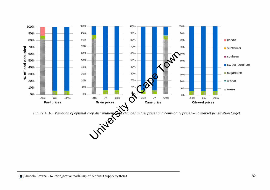
Thapelo Letete - Multiobjective modelling of biofuels supply systems 82
0%
10%
20%
30%
40%
50%
60%
70%
80%
90%
100%
-30% 0% +30%
Fuel prices
% o
f lan
d oc
cupi
ed
0%
10%
20%
30%
40%
50%
60%
70%
80%
90%
100%
-30% 0% +30%
Grain prices
0%
10%
20%
30%
40%
50%
60%
70%
80%
90%
100%
-30% 0% +30%
Cane price
0%
10%
20%
30%
40%
50%
60%
70%
80%
90%
100%
-30% 0% +30%
Oilseed prices
canola
sunflow er
soybean
sw eet_sorghum
sugarcane
w heat
maize
Figure 4. 18: Variation of optimal crop distributions with changes in fuel prices and commodity prices – no market penetration target
Univers
ity of
Cap
e Tow
n
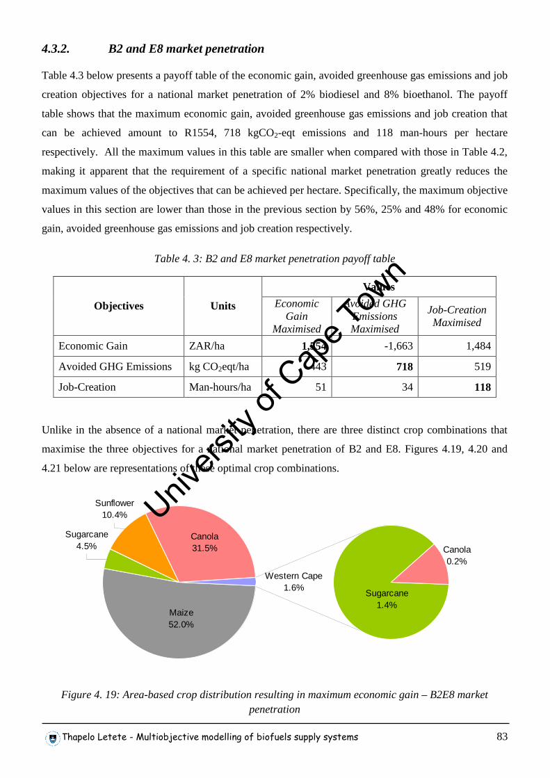
Thapelo Letete - Multiobjective modelling of biofuels supply systems 83
4.3.2. B2 and E8 market penetration
Table 4.3 below presents a payoff table of the economic gain, avoided greenhouse gas emissions and job
creation objectives for a national market penetration of 2% biodiesel and 8% bioethanol. The payoff
table shows that the maximum economic gain, avoided greenhouse gas emissions and job creation that
can be achieved amount to R1554, 718 kgCO2-eqt emissions and 118 man-hours per hectare
respectively. All the maximum values in this table are smaller when compared with those in Table 4.2,
making it apparent that the requirement of a specific national market penetration greatly reduces the
maximum values of the objectives that can be achieved per hectare. Specifically, the maximum objective
values in this section are lower than those in the previous section by 56%, 25% and 48% for economic
gain, avoided greenhouse gas emissions and job creation respectively.
Table 4. 3: B2 and E8 market penetration payoff table
Values
Objectives Units Economic Gain
Maximised
Avoided GHG Emissions Maximised
Job-Creation Maximised
Economic Gain ZAR/ha 1,554 -1,663 1,484
Avoided GHG Emissions kg CO2eqt/ha 443 718 519
Job-Creation Man-hours/ha 51 34 118
Unlike in the absence of a national market penetration, there are three distinct crop combinations that
maximise the three objectives for a national market penetration of B2 and E8. Figures 4.19, 4.20 and
4.21 below are representations of these optimal crop combinations.
Western Cape1.6%
Sugarcane1.4%
Canola0.2%
Canola31.5%
Sugarcane4.5%
Maize52.0%
Sunflower10.4%
Figure 4. 19: Area-based crop distribution resulting in maximum economic gain – B2E8 market
penetration
Univers
ity of
Cap
e Tow
n
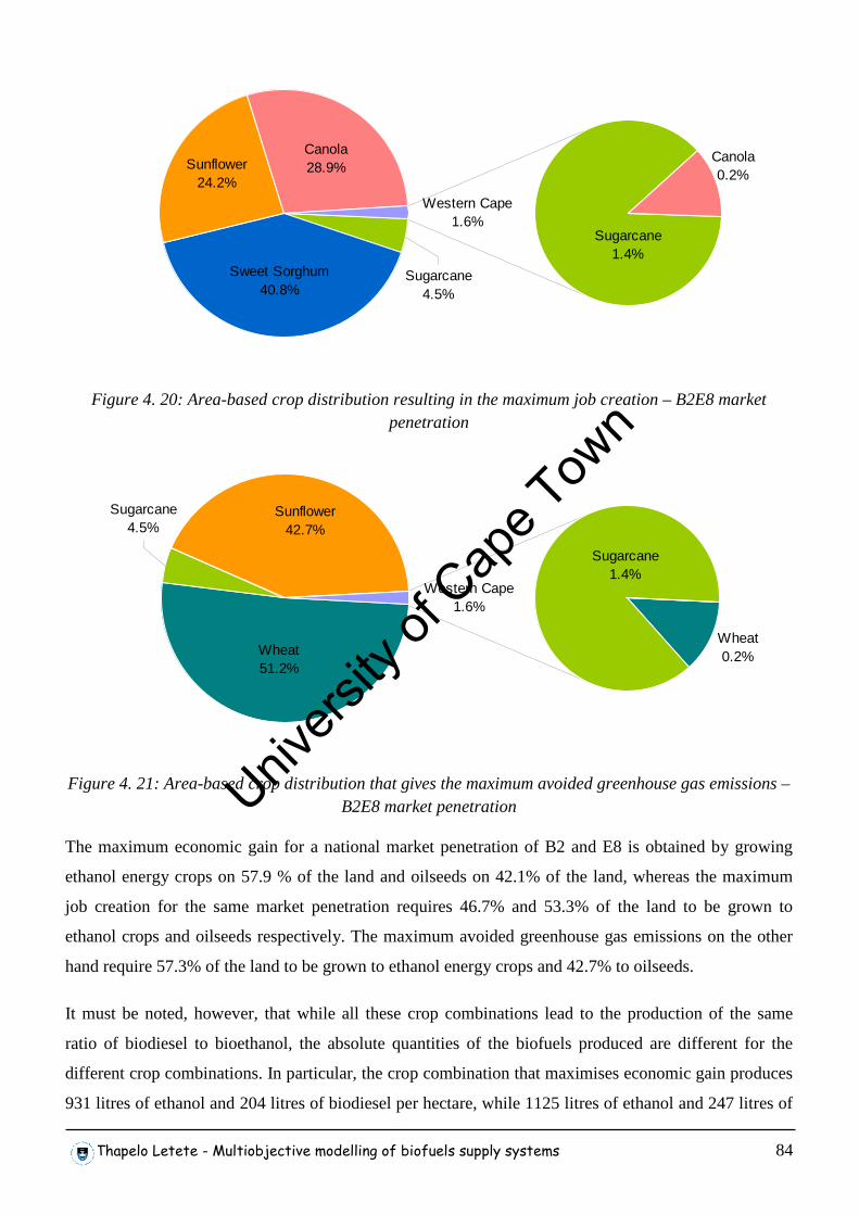
Thapelo Letete - Multiobjective modelling of biofuels supply systems 84
Sunflower24.2%
Sugarcane4.5%
Sweet Sorghum40.8%
Canola28.9%
Sugarcane1.4%
Canola0.2%
Western Cape1.6%
Figure 4. 20: Area-based crop distribution resulting in the maximum job creation – B2E8 market
penetration
Western Cape1.6%
Wheat0.2%
Sugarcane1.4%
Sugarcane4.5%
Wheat51.2%
Sunflower42.7%
Figure 4. 21: Area-based crop distribution that gives the maximum avoided greenhouse gas emissions –
B2E8 market penetration
The maximum economic gain for a national market penetration of B2 and E8 is obtained by growing
ethanol energy crops on 57.9 % of the land and oilseeds on 42.1% of the land, whereas the maximum
job creation for the same market penetration requires 46.7% and 53.3% of the land to be grown to
ethanol crops and oilseeds respectively. The maximum avoided greenhouse gas emissions on the other
hand require 57.3% of the land to be grown to ethanol energy crops and 42.7% to oilseeds.
It must be noted, however, that while all these crop combinations lead to the production of the same
ratio of biodiesel to bioethanol, the absolute quantities of the biofuels produced are different for the
different crop combinations. In particular, the crop combination that maximises economic gain produces
931 litres of ethanol and 204 litres of biodiesel per hectare, while 1125 litres of ethanol and 247 litres of
Univers
ity of
Cap
e Tow
n
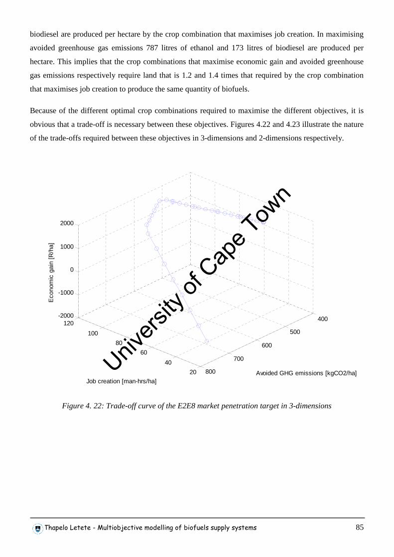
Thapelo Letete - Multiobjective modelling of biofuels supply systems 85
biodiesel are produced per hectare by the crop combination that maximises job creation. In maximising
avoided greenhouse gas emissions 787 litres of ethanol and 173 litres of biodiesel are produced per
hectare. This implies that the crop combinations that maximise economic gain and avoided greenhouse
gas emissions respectively require land that is 1.2 and 1.4 times that required by the crop combination
that maximises job creation to produce the same quantity of biofuels.
Because of the different optimal crop combinations required to maximise the different objectives, it is
obvious that a trade-off is necessary between these objectives. Figures 4.22 and 4.23 illustrate the nature
of the trade-offs required between these objectives in 3-dimensions and 2-dimensions respectively.
20
40
60
80
100
120400
500
600
700
800
-2000
-1000
0
1000
2000
Avoided GHG emissions [kgCO2/ha]Job creation [man-hrs/ha]
Eco
nom
ic g
ain
[R/h
a]
Figure 4. 22: Trade-off curve of the E2E8 market penetration target in 3-dimensions
Univers
ity of
Cap
e Tow
n
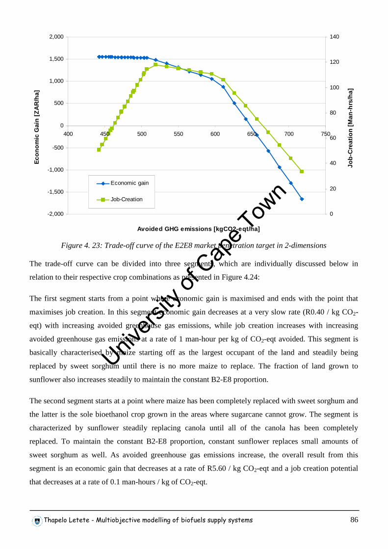
Thapelo Letete - Multiobjective modelling of biofuels supply systems 86
-2,000
-1,500
-1,000
-500
0
500
1,000
1,500
2,000
400 450 500 550 600 650 700 750
Avoided GHG emissions [kgCO2-eqt/ha]
Eco
nom
ic G
ain
[ZA
R/h
a]
0
20
40
60
80
100
120
140
Job-
Cre
atio
n [M
an-h
rs/h
a]
Economic gain
Job-Creation
Figure 4. 23: Trade-off curve of the E2E8 market penetration target in 2-dimensions
The trade-off curve can be divided into three segments, which are individually discussed below in
relation to their respective crop combinations as presented in Figure 4.24:
The first segment starts from a point where economic gain is maximised and ends with the point that
maximises job creation. In this segment economic gain decreases at a very slow rate (R0.40 / kg CO2-
eqt) with increasing avoided greenhouse gas emissions, while job creation increases with increasing
avoided greenhouse gas emissions at a rate of 1 man-hour per kg of CO2-eqt avoided. This segment is
basically characterised by maize starting off as the largest occupant of the land and steadily being
replaced by sweet sorghum until there is no more maize to replace. The fraction of land grown to
sunflower also increases steadily to maintain the constant B2-E8 proportion.
The second segment starts at a point where maize has been completely replaced with sweet sorghum and
the latter is the sole bioethanol crop grown in the areas where sugarcane cannot grow. The segment is
characterized by sunflower steadily replacing canola until all of the canola has been completely
replaced. To maintain the constant B2-E8 proportion, constant sunflower replaces small amounts of
sweet sorghum as well. As avoided greenhouse gas emissions increase, the overall result from this
segment is an economic gain that decreases at a rate of R5.60 / kg CO2-eqt and a job creation potential
that decreases at a rate of 0.1 man-hours / kg of CO2-eqt.
Univers
ity of
Cap
e Tow
n
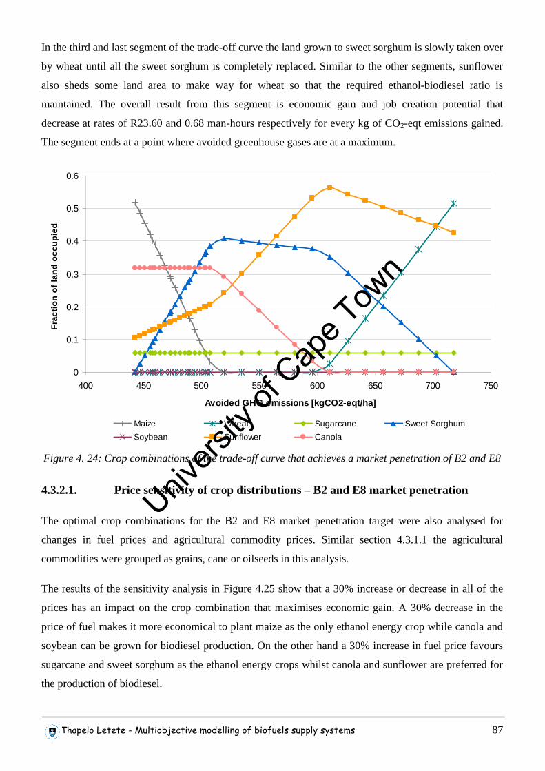
Thapelo Letete - Multiobjective modelling of biofuels supply systems 87
In the third and last segment of the trade-off curve the land grown to sweet sorghum is slowly taken over
by wheat until all the sweet sorghum is completely replaced. Similar to the other segments, sunflower
also sheds some land area to make way for wheat so that the required ethanol-biodiesel ratio is
maintained. The overall result from this segment is economic gain and job creation potential that
decrease at rates of R23.60 and 0.68 man-hours respectively for every kg of CO2-eqt emissions gained.
The segment ends at a point where avoided greenhouse gases are at a maximum.
0
0.1
0.2
0.3
0.4
0.5
0.6
400 450 500 550 600 650 700 750
Avoided GHG emissions [kgCO2-eqt/ha]
Fra
ctio
n of
land
occ
upie
d
Maize Wheat Sugarcane Sweet Sorghum
Soybean Sunflower Canola
Figure 4. 24: Crop combinations of the trade-off curve that achieves a market penetration of B2 and E8
4.3.2.1. Price sensitivity of crop distributions – B2 and E8 market penetration
The optimal crop combinations for the B2 and E8 market penetration target were also analysed for
changes in fuel prices and agricultural commodity prices. Similar section 4.3.1.1 the agricultural
commodities were grouped as grains, cane or oilseeds in this analysis.
The results of the sensitivity analysis in Figure 4.25 show that a 30% increase or decrease in all of the
prices has an impact on the crop combination that maximises economic gain. A 30% decrease in the
price of fuel makes it more economical to plant maize as the only ethanol energy crop while canola and
soybean can be grown for biodiesel production. On the other hand a 30% increase in fuel price favours
sugarcane and sweet sorghum as the ethanol energy crops whilst canola and sunflower are preferred for
the production of biodiesel.
Univers
ity of
Cap
e Tow
n
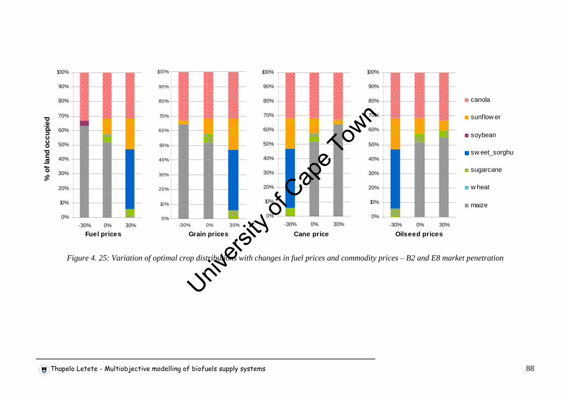
Thapelo Letete - Multiobjective modelling of biofuels supply systems 88
0%
10%
20%
30%
40%
50%
60%
70%
80%
90%
100%
-30% 0% 30%
Fuel prices
% o
f lan
d oc
cupi
ed
0%
10%
20%
30%
40%
50%
60%
70%
80%
90%
100%
-30% 0% 30%
Grain prices
0%
10%
20%
30%
40%
50%
60%
70%
80%
90%
100%
-30% 0% 30%
Cane price
0%
10%
20%
30%
40%
50%
60%
70%
80%
90%
100%
-30% 0% 30%
Oilseed prices
canola
sunflow er
soybean
sw eet_sorghu
sugarcane
w heat
maize
Figure 4. 25: Variation of optimal crop distributions with changes in fuel prices and commodity prices – B2 and E8 market penetration
Univers
ity of
Cap
e Tow
n
Thapelo Letete - Chapter 5: Maluti-a-Phofung Case Study 89
As with the results of section 4.3.1.1, a 30% decrease in the prices of grains has the same effect on the
optimal crop combination as a 30% increase in the price of cane and vice-versa. The decrease in grain
prices makes it more economical to grow maize as the only ethanol energy crop while the increase
makes cane crops the most economical options. In both of these cases canola and sunflower are the most
preferred biodiesel crops.
The results of the analysis also show that a 30% decrease in the prices of oilseeds has exactly the same
effect on the optimal crop combination as a 30% increase in fuel prices or a 30% increase in grain prices
or a 30% decrease in the price of cane crops – they all favour a combination of 5.9% sugarcane, 41.1%
sweet sorghum, 21.3% sunflower and 31.7% canola. This is behaviour that results from a decrease in
oilseed prices can be attributed to the fact that it leads to positive a positive economic gain for sunflower
biodiesel, and when combined with the already large economic gain of sweet sorghum ethanol, the result
is an overall economic gain that surpasses that of any of the combinations involving grain crops. An
increase in the oilseed prices on the other hand does not have significant effects on the optimal crop
combination.
4.4. Summary of key findings and outlook
The results of this chapter can be summarised as follows:
• All the biofuels analysed in this thesis show positive energy balances and energy balance ratios that
are greater than 1.
• The conversion of land to biofuel production results in a ‘once-off’ carbon debt which the biofuels
can only repay if their production and use avoid the emission of greenhouse gases in each year
subsequent to bringing that land into agricultural production. It was found that the production of
maize grain ethanol and sweet sorghum ethanol do not avoid greenhouse gas emissions under the
assumptions of this study, hence would be unable to repay the carbon debt. In the case of sweet
sorghum, the assumption of large transport distances associated with the distant location of currently
existing sugar mills could be reviewed, whereas in the case of maize, the use of fossil fuels in
processing would have to be stopped and replaced by a less greenhouse gas intensive way of
providing industrial heat.
• Economic gain and job creation are maximised by a common crop distribution but a trade-off is
required between these objectives and avoided green house gas emissions in the absence of national
biofuel market penetration targets. For a market penetration target of B2-E8, however, the three
objectives are maximised by different crop combinations, hence trade-offs are required between all
Univers
ity of
Cap
e Tow
n
Thapelo Letete - Chapter 5: Maluti-a-Phofung Case Study 90
three. Both of these cases show marked sensitivities to changes in agricultural commodity prices and
fuel prices.
This chapter has focused on the optimization of land use for biofuel production on a national scale. The
next chapter looks at how this model can be applied to a specific situation and be used to aid decision-
making at a local government level regarding biofuel production.
Univers
ity of
Cap
e Tow
n
Thapelo Letete - Chapter 5: Maluti-a-Phofung Case Study 91
5. MALUTI-A-PHOFUNG LOCAL GOVERNMENT CASE STUDY
In this chapter the use of multiobjective optimization to support decision-making in the development of
a biofuels industry is demonstrated at municipal level.
5.1. Area Description
Maluti-a-phofung is one of the five municipalities of the Thabo Mofutsanyana district, which is located
in the eastern part of the Free State province, bordering with the kwaZulu-Natal province to the east and
the Kingdom of Lesotho to the south. The Maluti-a-phofung municipality is home to 54% of the district
population, while covering only 16% of the district surface area, making it the third most populated area
in the Freestate at 87 people per km2 (Business Trust and DPLG, 2007). As shown in Figure 5.1 below
the municipality is characterized by three urban complexes around which the whole municipality
evolves: The Harrismith complex, Phuthaditjhaba-Qwaqwa complex and the Kestell complex (IDP,
2007).
The Harrismith complex is composed of the town of Harrismith and the two townships of Intabazwe and
Tsiame. It is located in the eastern central part of the municipality, around the intersection of the N3 and
N5 national roads connecting Durban with Johannesburg and Bloemfontein, respectively. According to
the local municipality, the complex derives much of its economic activity from this favourable position
at a major junction, its relative proximity to the export harbour of Durban, as well as the large and
relatively cheap labour force residing in the region. The town of Harrismith, which forms the economic
hub of the complex, is well-serviced in terms of infrastructure and housing, and therefore accommodates
the more affluent communities of the municipality. Intabazwe and Tsiame, on the other hand, are
characterized by low levels of infrastructure and employment. Intabazwe is a former African township
separated from the Harrismith CBD by a mountain and stream, while Tsiame is “a typical apartheid-
engineered dormitory town” located some 12km west of Harrismith.
The Phuthaditjhaba-Qwaqwa complex comprises of Qwaqwa - one of the former homelands which
became part of South Africa in 1994 (Appendix B) – and Phuthaditjhaba – its formal gateway and urban
component. The area of Qwaqwa outside Phuthaditjhaba is mostly composed of traditional and informal
villages, some of which are so remotely located that only a few rudimentary roads connect them to the
rest of the district. The complex is consequently by far the poorest and most densely populated in the
district.
Univers
ity of
Cap
e Tow
n
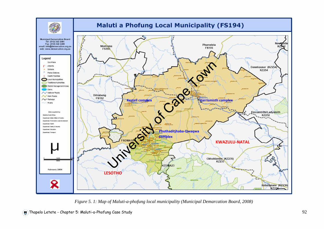
Thapelo Letete - Chapter 5: Maluti-a-Phofung Case Study 92
LESOTHO
KWAZULU-NATAL
Phuthaditjhaba-Qwaqwa
complex
Harrismisth complex Kestell complex
Figure 5. 1: Map of Maluti-a-phofung local municipality (Municipal Demarcation Board, 2008)
Univers
ity of
Cap
e Tow
n
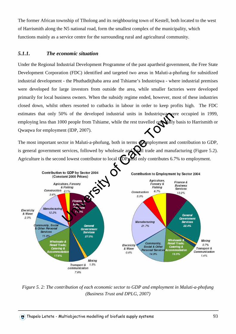
Thapelo Letete - Multiobjective modelling of biofuels supply systems 93
The former African township of Tlholong and its neighbouring town of Kestell, both located to the west
of Harrismith along the N5 national road, form the smallest complex of the municipality, which
functions mainly as a service centre for the surrounding rural and agricultural community.
5.1.1. The economic situation
Under the Regional Industrial Development Programme of the past apartheid government, the Free State
Development Corporation (FDC) identified and targeted two areas in Maluti-a-phofung for subsidized
industrial development - the Phuthaditjhaba area and Tshiame’s Industriqwa - where industrial premises
were developed for large investors from outside the area, while smaller factories were developed
primarily for local business owners. When the subsidy regime ended, however, most of these industries
closed down, whilst others resorted to cutbacks in labour in order to keep profits high. The FDC
estimates that only 50% of the developed industrial units in Industriqwa were occupied in 1999,
employing less than 1000 people from Tshiame, while the rest travelled on a daily basis to Harrismith or
Qwaqwa for employment (IDP, 2007).
The most important sector in Maluti-a-phofung, both in terms of employment and contribution to GDP,
is general government services, followed by wholesale and retail trade and manufacturing (Figure 5.2).
Agriculture is the second lowest contributor to local GDP, and only contributes 6.7% to employment.
Figure 5. 2: The contribution of each economic sector to GDP and employment in Maluti-a-phofung
(Business Trust and DPLG, 2007)
Univers
ity of
Cap
e Tow
n
Thapelo Letete - Multiobjective modelling of biofuels supply systems 94
According to Stats-SA (2008), only 22.6% of the potential workforce in Maluti-a-phofung is employed,
while over 80% live below the national poverty level (subsistence level) of R 19,200 per annum. For the
ten year period between 1995 and 2004, the GDP per capita of Maluti-a-phofung averaged R 6,860 (at
constant 2000 prices) - approximately 38% of the provincial average (Business Trust and DPLG, 2007).
In 2001, Maluti-a-phofung was declared one of the most severely impoverished areas in the country and
therefore, together with about 23 other regions in the country, was enrolled under two initiatives of the
state president –The Urban Renewal Programme (URP) and the Integrated Sustainable Rural
Development Programme (ISRDP) – created specifically to address underdevelopment in such areas
(Business Trust and DPLG, 2007).
5.1.2. The Agricultural situation
The Thabo Mofutsanyana district as a whole can be described as the most fertile region in the Freestate,
with a production capacity and gross income per hectare that are well above the provincial average. On
average, Maluti-a-phofung receives between 700 and 800 mm of rain per annum, mostly in the summer
seasons.
Similar to many parts of the country, Maluti-a-phofung is characterized by two agricultural practices;
commercial farming - which occurs in the flat land surrounding Harrismith and Kestell - and subsistence
farming, mainly in Phuthaditjhaba and the surrounding area of Qwaqwa. Maize, wheat, dry beans,
sunflower and soybeans are the most popular crops for commercial farmers, while subsistence farming
is mainly on livestock, poultry, grain sorghum and vegetables (Business Trust and DPLG, 2007). Grain
crops are sold to AFGRI silos and SASKO while cattle are sold at auctions held by co-operatives in the
district. Perennial grasses like sugarcane cannot thrive because of the high levels of frost that occur
during the winter seasons (Meyers, 2008).
Commercial farming is still dominated by white farmers in Maluti-a-phofung, partly because of the low
numbers of land claims in this area compared to other regions of the province. From the late 1980s to the
early 1990s, however, a total of 95,896 ha of land were awarded to 114 black emerging farmers in the
area between Kestell and Harrismith under the guidance of the Agricultural Development Agency of
Qwaqwa (Agriqwa) (Business Trust and DPLG, 2007). The Agriqwa scheme also involved setting up
three test farms which acted as support centres for these black farmers in terms of technical advice,
training, planning and funding. In 1995, however, this scheme was terminated by government, thus
taking away the much needed support for these emerging farmers. Because of lack of financial,
management and, in some cases, even technical skills, most of these farmers were left burdened with
debt and unable to effectively operate the farms.
Univers
ity of
Cap
e Tow
n
Thapelo Letete - Multiobjective modelling of biofuels supply systems 95
Many schemes have since been proposed by various institutions in an attempt to help the black emerging
farmers, including partnering with financial institutions like FNB, but failed in the end because they
only addressed the problem in part (Meyers, 2008). Since 2006 the following parallel schemes have
been tailor-made and adopted to address the problems of these emerging farmers:
i. The AFGRI Scheme: In this scheme AFGRI recruits and makes contracts with farmers, via an
independent agricultural advisor, to undertake all cultivation activities on the farm and then share
all profits 50:50 with the farmer. AFGRI insures and out-sources all farming activities from
independent and highly skilled contractors. By 2007 the scheme had attracted some 28 farmers,
owning a total of 2,680 ha of arable land, in Maluti-a-phofung. AFGRI’s plan is to grow maize
exclusively, and start rotating with soybean and sunflower only after 3-4 years (Ballod, 2008).
Because of the economies of scale, however, the scheme is only open to farmers with 50 ha of
arable crop land or more.
ii. Department of Agriculture’s cooperative scheme: In this scheme the black emerging farmers, the
subsistence farmers and some small-scale farmers (the latter have been awarded pieces of state-
owned farm land as caretakers) have been organized into co-operatives, and each co-operative has
been given a full set of agricultural machinery and implements by the district Department of
Agriculture. The machinery is rented out for a small fee to any farmer who needs to use it,
including co-operative members, to generate money for maintaining the machinery. The
Department of Agriculture further manages demonstration farms and occasionally holds technical
training workshops to support these farmers (Majake, 2008). According to the farmers (Moloi,
2008), this scheme has done very little to solve their problems because there are only a few sets of
agricultural machinery available yet all farmers often need to use them at the same time. The
limited number of agricultural extension officers and the lack of appropriate skills for most of the
extension officers have also contributed to the limited impact of this scheme.
While the two schemes have somewhat reduced the number of struggling black farmers in the area, they
have not solved the agricultural problems of the municipality. Many emerging and small scale farmers
are still left struggling because the co-operative scheme has failed them and they do not have the
minimum crop land requirement of 50 ha for the AFGRI scheme (Moloi, 2008). On the other hand,
many of those farmers who meet AFGRI’s minimum requirements have remained sceptical about the
scheme and opted to rather work their own land as far as they can (Makoele, 2008). In interviews, three
of these emerging and small-scale farmers in Maluti-a-phofung stated that most of them believe that the
failure of black farmers in the area is mostly due to racial discrimination at the AFGRI and SASKO
Univers
ity of
Cap
e Tow
n
Thapelo Letete - Multiobjective modelling of biofuels supply systems 96
silos, where their produce, mostly grain, is always labelled as inferior to that of their white counterparts
and therefore bought at lower prices (Ntholeng, 2008;Makoele, 2008;Macaphasa, 2008).
5.1.3. Integrated Development Planning
Maluti-a-phofung, like all other local municipalities in South Africa, is required by law to prepare an
Integrated Development Plan (IDP), following every Local Government election, to guide the new
Municipal Council throughout its five year term. The IDP acts as the principal strategic planning
instrument that guides and informs all planning, budgeting, management and decision-making in the
municipality (IDP, 2008).
Although the preparation of the IDP is primarily the responsibility of the municipal councillors and
municipal officers, the following stakeholders within Maluti-a-phofung are also involved to ensure the
relevance of the IDP as the municipality’s strategic plan (IDP, 2008):
• Civil Society: This group incorporates Ward committee representatives, NGO’s in the area,
community-based organisations and faith-based organizations.
• District municipality: These ensure that local municipal planning aligns well with district
planning and plans of other spheres of government
• Provincial government and Corporate Service Providers: The former ensure proper linkage
between national and local priorities while the latter contribute expertise and technical
knowledge. They also ensure that their 5 year plans are integrated into the municipality’s 5 year
capital programmes.
• External Support: Ithuteng Management Consultancy is usually engaged to provide
methodological and technical guidance to the IDP process, and to facilitate the planning of
workshops. They are also responsible for documenting the outcomes of all planning activities.
• The public: This is also involved through structured participation and various forms of media.
The IDP is reviewed on an annual basis to assess the municipality’s performance in the previous year, to
incorporate new information and changed circumstances and to reflect the budget for the new financial
year. The annual strategies for the different priorities of the municipality are also identified and laid out
in the form of projects which are assigned to the relevant departments for implementation. Because of
Maluti-a-Phofung’s limited annual revenue, however, the budget required for the implementation of all
the proposed projects is always much greater than the amount that can be allocated to them. Hence the
projects always need to be prioritised, with preference given to those that immediately address the basic
needs of the community and the well being of the people (Mothekhe, 2008).
Univers
ity of
Cap
e Tow
n
Thapelo Letete - Multiobjective modelling of biofuels supply systems 97
In Maluti-a-phofung’s 2008/2009 annual review of the IDP (2008), the Local Economic Development
and Poverty alleviation sector was by far the largest and most comprehensive; accounting for more than
59% of the budget required for the projects. As outlined in the IDP itself, the main objectives of this
sector are:
• To draw investment to the area
• To expand the agricultural and agro-processing sector in the region
• To expand the tourism sector in the region
• To expand the science and technology sector in the region
• To expand the mining and mineral beneficiation sector in the region
• To expand the manufacturing sector in the area
• To strengthen institutional capacity of SMME’s and increase the number of viable emerging
businesses
• To eradicate poverty
• To protect and secure the environment
According to Thamahane and Nhlapho (2008) the role of the Local Economic Development (LED)
office of the municipality in the proposed projects is simply to create a business environment and help
establish enterprises which should then be run by the relevant beneficiaries or, in some cases, appointed
contractors in the long run. In community-based projects the municipality usually remains involved
throughout the life-time of the project as an overseer and advisor.
5.2. Biofuels in Maluti-a-phofung
The Biofuels Industrial Strategy of the Republic of South Africa (DME, 2007) states that:
“The strategy targets areas of South Africa that are worst hit by poverty and deprivation. It
hopes to generate economic activity, mainly, in the former homelands. Furthermore, only
agricultural products grown in the previous homelands by historically disadvantaged farmers
will qualify for support.”
This means that the national biofuels strategy is basically an economic and agricultural development
programme tailor-made for areas like Maluti-a-phofung.
To achieve its purpose, especially in the agricultural sector, the strategy proposes that the existing
agricultural support programmes of the Department of Agriculture, such as the Comprehensive
Agricultural Support Programme (CASP), be used to support biofuel crops. In particular, it suggests that
Univers
ity of
Cap
e Tow
n
Thapelo Letete - Multiobjective modelling of biofuels supply systems 98
the budget of these programmes be increased and their focus be re-directed at capacitating emerging
farmers to fully utilize their land.
This section investigates practical ways in which the Maluti-a-phofung specifically can take part in the
development of a national biofuels industry based on the tools and the resources available to the
municipality.
5.2.1. Feedstock and land use
As shown in section 2.4, waste biomass is the most environmentally friendly and, therefore, most
preferable feedstock for biofuel production. In Maluti-a-Phofung the two largest potential sources of
waste biomass are the manufacturing industry and the agricultural industry:
• The most significant biomass wastes from the manufacturing sector are sawdust and wood off-cuts
from the four furniture-making factories in the municipality. These factory wastes, however, are
picked up in small vans and wheelbarrows by local residents and used as firewood. Saw dust is also
collected by chicken farmers in the area and used as an insulation material in the chicken sheds
(Kwaja Lounge Suits, 2008;Taurus and Tamasa Furnuture, 2008).
• In the agricultural sector, the grain stalks and bean straw that are left in the field after harvesting are
also potential feedstock for biofuels. The custom in the area, however, is to bring livestock to newly
harvested fields to feed on the stalks and straw, and the little that the animals leave behind is
ploughed back into the soil as a means of preserving nutrients (Meyers, 2008).
Therefore there is really no waste biomass available for biofuel production in the municipality. On the
other hand, there is plenty of underutilized land in Maluti-a-phofung that can be used for growing
energy crops as proposed in the biofuels strategy. The three categories of underutilized land available in
the area are as follows:
i. State land: According to the Department of Provincial and Local Government (Business Trust and
DPLG, 2007), there are 10,000 ha of underutilized semi-urban state land available for agriculture
in and around Phuthaditjhaba. This corresponds to about 3,900 ha of underutilized land suitable for
crop production (Appendix J).
ii. Land owned by black emerging farmers: Excluding the 2,680 ha that are currently under the
AFGRI scheme, an estimated 34,750 ha of crop land owned by black emerging farmers can be
classified under underutilized land in the municipality (Appendix J).
iii. Communal land: Most of the communal land in Maluti-a-phofung is not suitable crop cultivation,
and therefore, only used for raising livestock. The Department of Agriculture estimates that only
Univers
ity of
Cap
e Tow
n
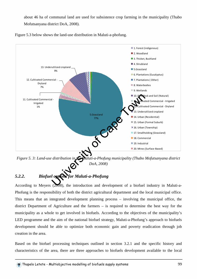
Thapelo Letete - Multiobjective modelling of biofuels supply systems 99
about 46 ha of communal land are used for subsistence crop farming in the municipality (Thabo
Mofutsanyana district DoA, 2008).
Figure 5.3 below shows the land-use distribution in Maluti-a-phofung.
5.Grassland
77%
13. Underutilized cropland
9%
12. Cultivated Commercial -
Dryland
7%
11. Cultivated Commercial -
Irrigated
1%
1. Forest (indigenous)
2. Woodland
3. Thicket, Bushland
4. Shrubland
5.Grassland
6. Plantations (Eucalyptus)
7. Plantations ( Other)
8. Waterbodies
9. Wetlands
10. Bare Rock and Soil (Natural)
11. Cultivated Commercial - Irrigated
12. Cultivated Commercial - Dryland
13. Underutilized cropland
14. Urban (Residential)
15. Urban (Formal Suburb)
16. Urban (Township)
17. Smallholding (Grassland)
18. Commercial
19. Industrial
20. Mines (Surface-Based)
Figure 5. 3: Land-use distribution in the Maluti-a-Phofung municipality (Thabo Mofutsanyana district
DoA, 2008)
5.2.2. Biofuel options for Maluti-a-Phofung
According to Meyers (2008), the introduction and development of a biofuel industry in Maluti-a-
Phofung is the responsibility of both the district agricultural department and the local municipal office.
This means that an integrated development planning process – involving the municipal office, the
district Department of Agriculture and the farmers – is required to determine the best way for the
municipality as a whole to get involved in biofuels. According to the objectives of the municipality’s
LED programme and the aim of the national biofuel strategy, Maluti-a-Phofung’s approach to biofuels
development should be able to optimize both economic gain and poverty eradication through job
creation in the area.
Based on the biofuel processing techniques outlined in section 3.2.1 and the specific history and
characteristics of the area, there are three approaches to biofuels development available to the local
Univers
ity of
Cap
e Tow
n
Thapelo Letete - Multiobjective modelling of biofuels supply systems 100
municipality of Maluti-a-phofung; the biodiesel-only approach, the bioethanol-only approach or a
combination of the two approaches.
5.2.2.1. Biodiesel-only approach
In line with the municipality’s objective of promoting local agro-processing, a biodiesel processing plant
could be established within the Maluti-a-phofung area through the Local Economic Development (LED)
programme. Similar to other LED projects, the daily operations of the plant would be undertaken by
either an appointed local contractor or, more preferably, a co-operative of farmers, while the municipal
office and the district Department of Agriculture would simply oversee plant activities and offer
technical advice respectively. In this approach all the available underutilized land would be used
exclusively for growing one or both of the oil crops which are most familiar to the local farmers –
soybean and sunflower – for biodiesel production. The biodiesel would then be delivered to the regional
blending station while the oil meals would either be sold to the local farmers or marketed outside the
municipality depending on the market.
This approach ensures that the entire supply-chain of the biofuel is confined within the limits of the
municipality; thus, making Maluti-a-phofung an “exporter” of finished products. The approach also
offers the municipality full control over the activities of the supply chain.
5.2.2.2. Bioethanol-only approach
Of the crops considered in this study, maize and wheat are the most appropriate for a bioethanol
programme in Maluti-a-phofung. While the climatic conditions of the area prohibit the cultivation of
sugarcane completely, the farmers may, however, use their familiarity with grain sorghum to grow sweet
sorghum. These energy crops could be grown on the underutilized land available in the municipality and
then sent to the appropriate bioethanol plants, outside the municipality, for processing. Based on the
bioethanol plant distribution shown in Figure 3.2, the closest grain processing ethanol plant to Maluti-a-
phofung would be in Bethlehem, while UCL Company in kwaZulu-Natal is the closest cane processing
plant.
In this approach, only the agricultural section of the bioethanol supply chain and the transportation of
crops to processing plants are within the boundaries of the municipality, while rest of the activities occur
outside the municipality. Although this approach is less demanding to the municipality in financial and
administrative terms, it also offers the municipality very little control over the supply chain as a whole.
5.2.2.3. Biodiesel and Bioethanol approach
This is basically a combination of the biodiesel-only approach and the bioethanol-only approach. Here a
biodiesel plant would be established within the municipality through the LED programme, but the
Univers
ity of
Cap
e Tow
n
Thapelo Letete - Multiobjective modelling of biofuels supply systems 101
available land would be used to grow both oil crops and bioethanol crops. The processing of the
bioethanol crops would be done in Bethlehem and kwaZulu-Natal as in the bioethanol approach.
The major drawback of this approach is that the operation and sustainability of the biodiesel plant will
be strongly influenced by agricultural commodity prices; in the years when the bioethanol energy crops
are fetching good prices or the oil crops are fetching poor prices, the farmers will revert to bioethanol
crops, leaving the biodiesel plant without feedstock, regardless of whether the economics of biodiesel
production may have changed or not.
5.3. The Decision Support System
This section presents a Decision Support System (DSS) that can be used by Maluti-a-phofung’s IDP
team to decide how the underutilized agricultural land available in the area could best be used for
biofuels production such that two of the municipality’s top objectives – local economic development and
job-creation – are maximised.
Two scenarios are considered in this case-study: the first one is termed the “All-crops” scenario where
sweet sorghum is introduced to the farmers as an energy crop that competes with the four energy crops –
maize, wheat, soybean and sunflower – that are already grown in the area, and the second, termed the
“four-crop” scenario, is where the farmers are not willing to take chances with sweet sorghum and
decide to stick to the four crops that they are already familiar with.
5.3.1. DSS Model Equations
5.3.1.1. Economic gain in Maluti-a-Phofung
The first objective – economic gain – is defined here as the net financial gain made by the area of
Maluti-a-Phofung as a whole due to the establishment of a local biofuels programme:
I.e. Economic gain = Net profit made in presence – Net profit made in absence of biofuel programme of biofuel programme
While only a certain percentage of the available agricultural land is currently utilized for production into
the food market, it is assumed here that the farmers will be able to fully utilize the land under the biofuel
programme as argued by the Biofuels strategy. Assuming, therefore, that the processing plants buy the
crops from the farmers at market price, the economic gain from the biodiesel supply chain is simply the
net profit made by the processing plant plus the extra revenue made by the farmers from utilizing the
land fully.
Univers
ity of
Cap
e Tow
n
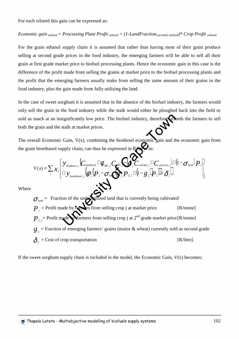
Thapelo Letete - Multiobjective modelling of biofuels supply systems 102
For each oilseed this gain can be expressed as:
Economic gain oilseed = Processing Plant Profit oilseed + (1-LandFractioncurrently utilized)* Crop Profit oilseed.
For the grain ethanol supply chain it is assumed that rather than having most of their grain produce
selling at second grade prices in the food industry, the emerging farmers will be able to sell all their
grain at first grade market price to biofuel processing plants. Hence the economic gain in this case is the
difference of the profit made from selling the grains at market price to the biofuel processing plants and
the profit that the emerging farmers usually make from selling the same amount of their grains in the
food industry, plus the gain made from fully utilizing the land.
In the case of sweet sorghum it is assumed that in the absence of the biofuel industry, the farmers would
only sell the grain in the food industry while the stalk would either be ploughed back into the field or
sold as snack at an insignificantly low price. The biofuel industry, therefore, affords the farmers to sell
both the grain and the stalk at market prices.
The overall Economic Gain, V(x), combining the biodiesel economic gain and the economic gain from
the grain bioethanol supply chain, can thus be expressed in R/ha/yr as:
( ) ( )( )( )( )( )( )∑
−−+−+
−++−+=
jjjjlandjjjbioethanol
jlandjprocessjmarketjjBPjBPbiodieseljbiodiesel
j
PgPgPyPCCCCy
xxVδσφ
σφφ2,22,
,,,,,
1
1)(
Where
σ land= Fraction of the underutilized land that is currently being cultivated
P j = Profit made by farmers from selling crop j at market price [R/tonne]
P j,2= Profit made by farmers from selling crop j at 2nd grade market price [R/tonne]
g2 = Fraction of emerging farmers’ grains (maize & wheat) currently sold as second grade
δ j = Cost of crop transportation [R/litre].
If the sweet sorghum supply chain is included in the model, the Economic Gain, V(x) becomes:
Univers
ity of
Cap
e Tow
n
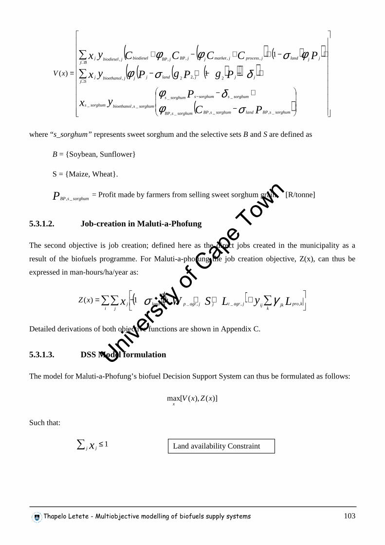
Thapelo Letete - Multiobjective modelling of biofuels supply systems 103
( ) ( )( )( )( )( )( )
( )
−
+−
+−−+−
+−++−+
=
−
∈
∈
∑
∑
PC
Pyx
PgPgPyx
PCCCCyx
sorghumsBPlandsorghumsBPsorghumsBP
sorghumssorghumssorghums
sorghumsbioethanolsorghums
jjjlandjjSj
jbioethanolj
BjjjlandjprocessjmarketjjBPjBPbiodieseljbiodieselj
xV
_,_,_,
__
_,_
2,22,
,,,,,
1
1
)(
σφδφ
δσφφσφφ
where “s_sorghum” represents sweet sorghum and the selective sets B and S are defined as
B = {Soybean, Sunflower}
S = {Maize, Wheat}.
P sorghumsBP _, = Profit made by farmers from selling sweet sorghum grain [R/tonne]
5.3.1.2. Job-creation in Maluti-a-Phofung
The second objective is job creation; defined here as the direct jobs created in the municipality as a
result of the biofuels programme. For Maluti-a-phofung the job creation objective, Z(x), can thus be
expressed in man-hours/ha/year as:
( )( )∑∑ ∑
++⋅⋅−=i j k
kprojkijjagrtjjagrplandj LyLSWx hxZ,,_,_
1)( γσ
Detailed derivations of both objective functions are shown in Appendix C.
5.3.1.3. DSS Model formulation
The model for Maluti-a-Phofung’s biofuel Decision Support System can thus be formulated as follows:
)](),([max xZxVx
Such that:
1≤∑ j jx Land availability Constraint
Univers
ity of
Cap
e Tow
n
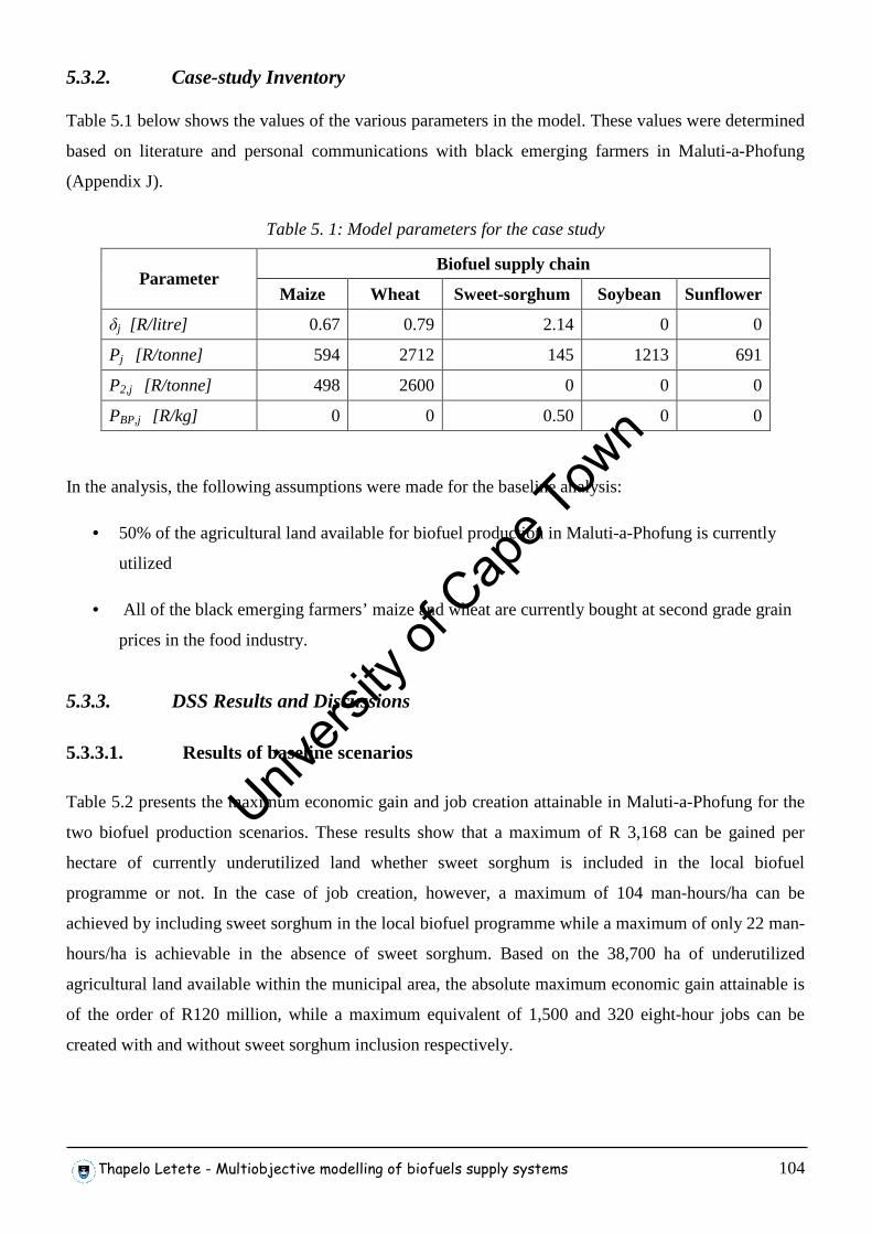
Thapelo Letete - Multiobjective modelling of biofuels supply systems 104
5.3.2. Case-study Inventory
Table 5.1 below shows the values of the various parameters in the model. These values were determined
based on literature and personal communications with black emerging farmers in Maluti-a-Phofung
(Appendix J).
Table 5. 1: Model parameters for the case study
Biofuel supply chain Parameter
Maize Wheat Sweet-sorghum Soybean Sunflower
δj [R/litre] 0.67 0.79 2.14 0 0
Pj [R/tonne] 594 2712 145 1213 691
P2,j [R/tonne] 498 2600 0 0 0
PBP,j [R/kg] 0 0 0.50 0 0
In the analysis, the following assumptions were made for the baseline analysis:
• 50% of the agricultural land available for biofuel production in Maluti-a-Phofung is currently
utilized
• All of the black emerging farmers’ maize and wheat are currently bought at second grade grain
prices in the food industry.
5.3.3. DSS Results and Discussions
5.3.3.1. Results of baseline scenarios
Table 5.2 presents the maximum economic gain and job creation attainable in Maluti-a-Phofung for the
two biofuel production scenarios. These results show that a maximum of R 3,168 can be gained per
hectare of currently underutilized land whether sweet sorghum is included in the local biofuel
programme or not. In the case of job creation, however, a maximum of 104 man-hours/ha can be
achieved by including sweet sorghum in the local biofuel programme while a maximum of only 22 man-
hours/ha is achievable in the absence of sweet sorghum. Based on the 38,700 ha of underutilized
agricultural land available within the municipal area, the absolute maximum economic gain attainable is
of the order of R120 million, while a maximum equivalent of 1,500 and 320 eight-hour jobs can be
created with and without sweet sorghum inclusion respectively.
Univers
ity of
Cap
e Tow
n
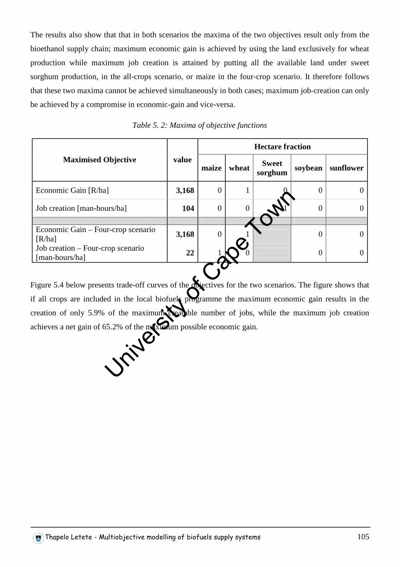
Thapelo Letete - Multiobjective modelling of biofuels supply systems 105
The results also show that that in both scenarios the maxima of the two objectives result only from the
bioethanol supply chain; maximum economic gain is achieved by using the land exclusively for wheat
production while maximum job creation is attained by putting all the available land under sweet
sorghum production, in the all-crops scenario, or maize in the four-crop scenario. It therefore follows
that these two maxima cannot be achieved simultaneously in both cases; maximum job-creation can only
be achieved by a compromise in economic-gain and vice-versa.
Table 5. 2: Maxima of objective functions
Hectare fraction
Maximised Objective value maize wheat Sweet
sorghum soybean sunflower
Economic Gain [R/ha] 3,168 0 1 0 0 0
Job creation [man-hours/ha] 104 0 0 1 0 0
Economic Gain – Four-crop scenario [R/ha]
3,168 0 1 0 0
Job creation – Four-crop scenario [man-hours/ha]
22 1 0 0 0
Figure 5.4 below presents trade-off curves of the objectives for the two scenarios. The figure shows that
if all crops are included in the local biofuels programme the maximum economic gain results in the
creation of only 5.9% of the maximum creatable number of jobs, while the maximum job creation
achieves a net gain of 65.2% of the maximum possible economic gain.
Univers
ity of
Cap
e Tow
n
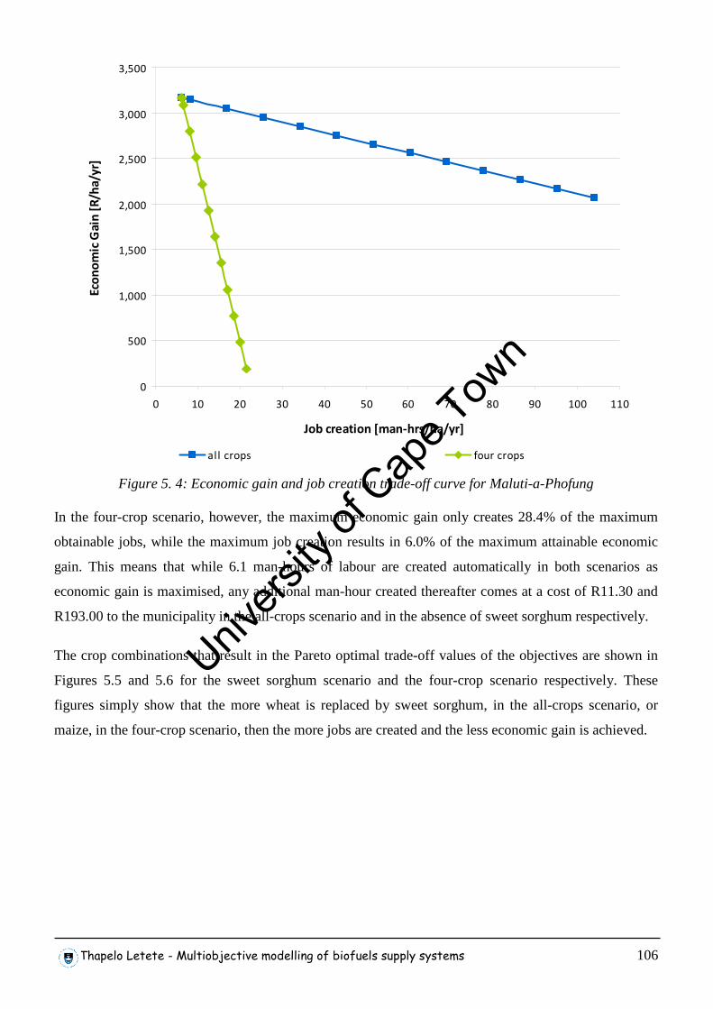
Thapelo Letete - Multiobjective modelling of biofuels supply systems 106
0
500
1,000
1,500
2,000
2,500
3,000
3,500
0 10 20 30 40 50 60 70 80 90 100 110
Job creation [man-hrs/ha/yr]
Eco
no
mic
Ga
in [
R/h
a/y
r]
all crops four crops
Figure 5. 4: Economic gain and job creation trade-off curve for Maluti-a-Phofung
In the four-crop scenario, however, the maximum economic gain only creates 28.4% of the maximum
obtainable jobs, while the maximum job creation results in 6.0% of the maximum attainable economic
gain. This means that while 6.1 man-hours of labour are created automatically in both scenarios as
economic gain is maximised, any additional man-hour created thereafter comes at a cost of R11.30 and
R193.00 to the municipality in the all-crops scenario and in the absence of sweet sorghum respectively.
The crop combinations that result in the Pareto optimal trade-off values of the objectives are shown in
Figures 5.5 and 5.6 for the sweet sorghum scenario and the four-crop scenario respectively. These
figures simply show that the more wheat is replaced by sweet sorghum, in the all-crops scenario, or
maize, in the four-crop scenario, then the more jobs are created and the less economic gain is achieved.
Univers
ity of
Cap
e Tow
n
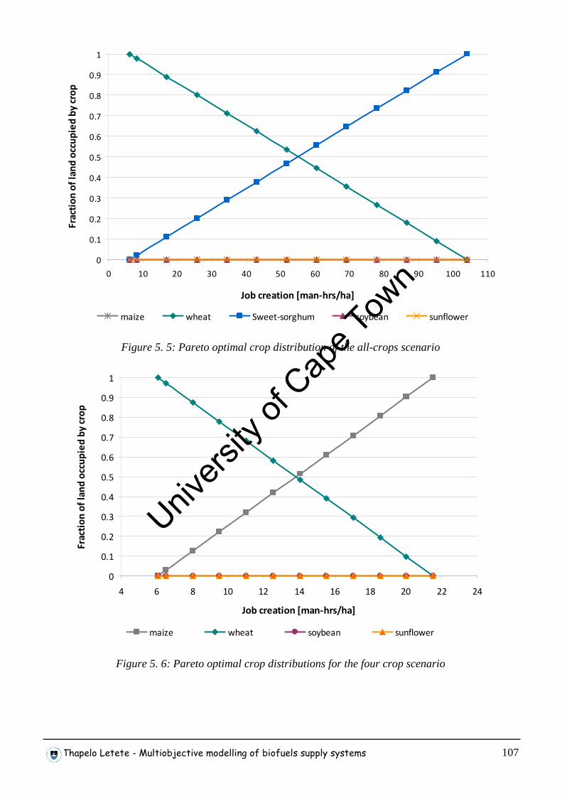
Thapelo Letete - Multiobjective modelling of biofuels supply systems 107
0
0.1
0.2
0.3
0.4
0.5
0.6
0.7
0.8
0.9
1
0 10 20 30 40 50 60 70 80 90 100 110
Job creation [man-hrs/ha]
Fra
ctio
n o
f la
nd
occ
up
ied
by
cro
p
maize wheat Sweet-sorghum soybean sunflower
Figure 5. 5: Pareto optimal crop distribution of the all-crops scenario
0
0.1
0.2
0.3
0.4
0.5
0.6
0.7
0.8
0.9
1
4 6 8 10 12 14 16 18 20 22 24
Job creation [man-hrs/ha]
Fra
ctio
n o
f la
nd
occ
up
ied
by
cro
p
maize wheat soybean sunflower
Figure 5. 6: Pareto optimal crop distributions for the four crop scenario
Univers
ity of
Cap
e Tow
n
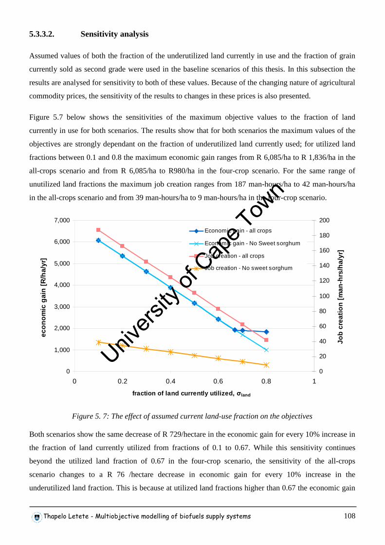
Thapelo Letete - Multiobjective modelling of biofuels supply systems 108
5.3.3.2. Sensitivity analysis
Assumed values of both the fraction of the underutilized land currently in use and the fraction of grain
currently sold as second grade were used in the baseline scenarios of this thesis. In this subsection the
results are analysed for sensitivity to both of these values. Because of the changing nature of agricultural
commodity prices, the sensitivity of the results to changes in these prices is also presented.
Figure 5.7 below shows the sensitivities of the maximum objective values to the fraction of land
currently in use for both scenarios. The results show that for both scenarios the maximum values of the
objectives are strongly dependant on the fraction of underutilized land currently used; for utilized land
fractions between 0.1 and 0.8 the maximum economic gain ranges from R 6,085/ha to R 1,836/ha in the
all-crops scenario and from R 6,085/ha to R980/ha in the four-crop scenario. For the same range of
unutilized land fractions the maximum job creation ranges from 187 man-hours/ha to 42 man-hours/ha
in the all-crops scenario and from 39 man-hours/ha to 9 man-hours/ha in the four-crop scenario.
0
1,000
2,000
3,000
4,000
5,000
6,000
7,000
0 0.2 0.4 0.6 0.8 1
fraction of land currently utilized, σland
econ
omic
gai
n [R
/ha/
yr]
0
20
40
60
80
100
120
140
160
180
200
Job
cre
atio
n [m
an-h
rs/h
a/yr
]
Economic gain - all crops
Economic gain - No Sweet sorghum
Job creation - all crops
Job creation - No sweet sorghum
Figure 5. 7: The effect of assumed current land-use fraction on the objectives
Both scenarios show the same decrease of R 729/hectare in the economic gain for every 10% increase in
the fraction of land currently utilized from fractions of 0.1 to 0.67. While this sensitivity continues
beyond the utilized land fraction of 0.67 in the four-crop scenario, the sensitivity of the all-crops
scenario changes to a R 76 /hectare decrease in economic gain for every 10% increase in the
underutilized land fraction. This is because at utilized land fractions higher than 0.67 the economic gain
Univers
ity of
Cap
e Tow
n
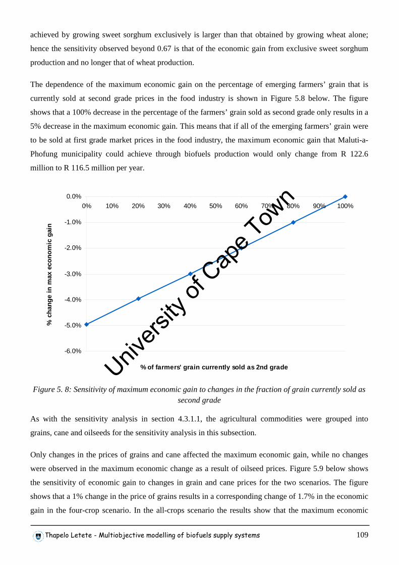
Thapelo Letete - Multiobjective modelling of biofuels supply systems 109
achieved by growing sweet sorghum exclusively is larger than that obtained by growing wheat alone;
hence the sensitivity observed beyond 0.67 is that of the economic gain from exclusive sweet sorghum
production and no longer that of wheat production.
The dependence of the maximum economic gain on the percentage of emerging farmers’ grain that is
currently sold at second grade prices in the food industry is shown in Figure 5.8 below. The figure
shows that a 100% decrease in the percentage of the farmers’ grain sold as second grade only results in a
5% decrease in the maximum economic gain. This means that if all of the emerging farmers’ grain were
to be sold at first grade market prices in the food industry, the maximum economic gain that Maluti-a-
Phofung municipality could achieve through biofuels production would only change from R 122.6
million to R 116.5 million per year.
-6.0%
-5.0%
-4.0%
-3.0%
-2.0%
-1.0%
0.0%
0% 10% 20% 30% 40% 50% 60% 70% 80% 90% 100%
% of farmers' grain currently sold as 2nd grade
% c
hang
e in
max
eco
nom
ic g
ain
Figure 5. 8: Sensitivity of maximum economic gain to changes in the fraction of grain currently sold as second grade
As with the sensitivity analysis in section 4.3.1.1, the agricultural commodities were grouped into
grains, cane and oilseeds for the sensitivity analysis in this subsection.
Only changes in the prices of grains and cane affected the maximum economic gain, while no changes
were observed in the maximum economic change as a result of oilseed prices. Figure 5.9 below shows
the sensitivity of economic gain to changes in grain and cane prices for the two scenarios. The figure
shows that a 1% change in the price of grains results in a corresponding change of 1.7% in the economic
gain in the four-crop scenario. In the all-crops scenario the results show that the maximum economic
Univers
ity of
Cap
e Tow
n
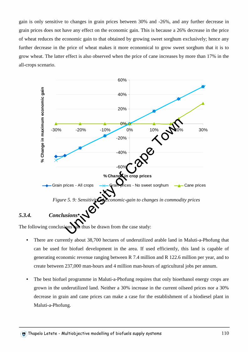
Thapelo Letete - Multiobjective modelling of biofuels supply systems 110
gain is only sensitive to changes in grain prices between 30% and -26%, and any further decrease in
grain prices does not have any effect on the economic gain. This is because a 26% decrease in the price
of wheat reduces the economic gain to that obtained by growing sweet sorghum exclusively; hence any
further decrease in the price of wheat makes it more economical to grow sweet sorghum that it is to
grow wheat. The latter effect is also observed when the price of cane increases by more than 17% in the
all-crops scenario.
-60%
-40%
-20%
0%
20%
40%
60%
-30% -20% -10% 0% 10% 20% 30%
% Change in crop prices
% C
hang
e in
max
imum
eco
nom
ic g
ain
Grain prices - All crops Grain prices - No sweet sorghum Cane prices
Figure 5. 9: Sensitivity of Economic-gain to changes in commodity prices
5.3.4. Conclusions
The following conclusions can thus be drawn from the case study:
• There are currently about 38,700 hectares of underutilized arable land in Maluti-a-Phofung that
can be used for biofuel development in the area. If used efficiently, this land is capable of
generating economic revenue ranging between R 7.4 million and R 122.6 million per year, and to
create between 237,000 man-hours and 4 million man-hours of agricultural jobs per annum.
• The best biofuel programme in Maluti-a-Phofung requires that only bioethanol energy crops are
grown in the underutilized land. Neither a 30% increase in the current oilseed prices nor a 30%
decrease in grain and cane prices can make a case for the establishment of a biodiesel plant in
Maluti-a-Phofung.
Univers
ity of
Cap
e Tow
n
Thapelo Letete - Multiobjective modelling of biofuels supply systems 111
• Of the energy crops currently grown in Maluti-a-Phofung, wheat results in the largest net
financial gain for the area while maize creates the largest number of jobs for biofuel production.
The inclusion of sweet sorghum in a biofuels programme in Maluti-a-phofung has the potential
of creating up to 5 times more jobs in the area than only using the four energy crops familiar to
the local farmers.
Univers
ity of
Cap
e Tow
n
Thapelo Letete - Multiobjective modelling of biofuels supply systems 112
6. CONCLUSIONS AND RECOMMENDATIONS
This thesis set out to analyse and to compare the land use options offered by different bioenergy crops
and technologies available to South Africa for the development of an agriculture-based biofuels
industry. In this chapter the findings of the preceding chapters are recalled to determine how well the
aims of the study have been met, to draw conclusions in line with the key questions and to make
recommendations for further research.
A review of relevant literature revealed that more than half of the global potential of biomass
contribution to the energy sector rests in sub-Saharan Africa, and that the extent to which it can be
unlocked is greatly dependant on the location, choice of feedstock and method of production. Literature
also showed that biofuels are a potential low-carbon energy source, but whether they actually offer the
carbon savings depends on how they are produced, and life-cycle assessment methods were found to be
the right tools for analysing the sustainability of biofuel supply chains. It was also found that land use
change and deforestation for biofuel production strongly influence the success and sustainability of
bioenergy systems, and that their effects should always be taken into account in analysing the
environmental and social impacts of bioenergy systems from a life-cycle perspective.
The literature review further revealed that while energy modelling can be used to analyse bioenergy
systems from an economic viewpoint only and life-cycle assessment tools can be adequately used to
analyse their social and environmental aspects, multiobjective optimization is the best method for
integrated analysis of all three dimensions.
Chapter 3 then described the system under study in detail, together with the developed multiobjective
optimization model. This model simultaneously maximises three objectives; economic gain by the
processing plant, direct job creation and greenhouse gas emissions avoided by using the biofuels, all at
minimal use of agricultural land. These objectives were chosen as the most outstanding economic, social
and environmental objectives respectively for the establishment of a biofuels industry in South Africa.
First presented in chapter 4 are the results of energy balance analyses of the different biofuel supply
chains. The results showed that the South African production of maize grain ethanol, wheat grain
ethanol, sugarcane ethanol, sweet sorghum ethanol, soybean biodiesel, sunflower biodiesel and canola
biodiesel all result in net energy gains. Sugarcane ethanol was found to have the highest effectiveness of
biofuel production with a Net Energy Balance of 73 GJ/ha/yr and the highest return on energy input of
3.72, while maize grain ethanol was the poorest in both cases with 6 GJ/ha/yr and 1.20 respectively. The
main reason for the poor performance of maize grain ethanol was found to be the large quantities of coal
and electricity required for steam generation and DDGS drying during processing.
Univers
ity of
Cap
e Tow
n
Thapelo Letete - Multiobjective modelling of biofuels supply systems 113
For both starch-based ethanol and biodiesel, the largest contribution of post-harvest energy inputs is
from the fossil energy used in processing the crops, hence the use of renewable energy sources for
powering all biofuel plants should be strongly emphasised in future work.
Chapter 4 also presented the environmental effects of land use change for biofuels production. The
results showed that bringing land that has not been cultivated for a period of two years to agricultural
production results in a carbon debt of about 13,900 kgCO2/ha, which the biofuels can only repay if their
production avoid the emission of greenhouse gases in each subsequent year. In terms of ability to repay
this debt, sugarcane ethanol was found to have the highest ability with a repayment period of only 3
years; while maize grain ethanol and sweet sorghum ethanol would not be able repay the debt under the
assumptions of this study. In the case of sweet sorghum ethanol, this is due to the assumption of large
transport distances associated with the distant location of currently existing sugar mills. The use of sweet
sorghum ethanol was found to be able to avoid greenhouse gas emissions only if the sorghum is grown
within return transportation distances of 442 km of the processing plant. As in the energy balance
analysis, the poor performance by maize grain ethanol here was found to be the fossil energy used in
processing, which would have to be replaced by a less greenhouse gas intensive way of providing
industrial heat if greenhouse gas emissions are to be avoided.
Presented last in chapter 4 were the results of the multiobjective model. Here scenarios of no targeted
national market penetration and a national market penetration target of 2% biodiesel and 8% bioethanol
were analysed and the following findings were presented:
• It was found that sugarcane is the most preferable crop for maximising all three objectives
wherever it can grow throughout the country, in the absence of a national market penetration
target. In the Western Cape areas where sugarcane cannot grow, canola is the most preferred for
maximising avoided greenhouse gas emissions and job creation. For maximising economic gain
in these areas, however, canola is only better than wheat but it is actually more economical to
leave the land uncultivated. In the areas outside the Western Cape where sugarcane cannot grow
sweet sorghum is the most preferred for maximizing both economic gain and job creation, while
sunflower and canola are the most preferred and second most preferred crops respectively for
maximizing avoided greenhouse gas emissions.
• The results further revealed that in the absence of a market penetration target trade-offs are
required between avoided greenhouse gas emissions and economic gain or job creation, and
these can be achieved by varying the fractions of sweet sorghum, sunflower and canola grown.
Under these conditions, an estimated 47 kg of CO2-eqt emissions are avoided freely per hectare
Univers
ity of
Cap
e Tow
n
Thapelo Letete - Multiobjective modelling of biofuels supply systems 114
as economic gain and job creation are maximised but any additional kilogram of CO2-eqt
emissions avoided thereafter comes at a cost of R4.50 and 0.2 man-hours.
• In the presence of a national market penetration of 2% biodiesel and 8% bioethanol the three
objectives are maximized by three distinct crop combinations. Economic gain is maximized by
growing as much sugarcane as possible for ethanol production and as much canola as possible
where sugarcane cannot be grown and then supplementing them with maize and sunflower
respectively to achieve the required ratio. Job creation is maximised by the same distribution
except that sweet sorghum instead of maize supplements sugarcane. Avoided greenhouse gas
emissions, on the other hand, is maximized by growing as much sugarcane as possible for
ethanol production and then balancing between sunflower for biodiesel production and wheat for
ethanol production to achieve the desired proportion. In terms of the quantities of biofuels
produced from each hectare, the crop combination that maximises job creation was found to give
the highest value, followed by the combination that maximises economic gain.
• These varying crop combinations imply that trade-offs are indeed required between these three
objectives. The results showed that the trade-off curve in the presence of a market penetration is
essentially made up of three segments; in the first segment the trade-off is between sweet
sorghum and maize for ethanol production, in the second segment sunflower and canola compete
for biodiesel production whilst in the last segment the trade-off is between sweet sorghum and
wheat for ethanol production. It was observed that moving from the first segment to the last
increases the greenhouse gas emissions avoided while reducing economic gain and job creation.
• Analysis of the sensitivity of these results to changes in fuel prices, grain prices, cane prices and
oilseed prices showed that economic gain in the presence of a national market target is sensitive
to changes in all these prices, while in the absence of a market target the economic gain is only
sensitive to changes in the first three.
While the qualitative findings of this modelling exercise are believed to be precise, the quantitative
results can be improved by using crop yields, agricultural practices and land suitabilities of crops
specific to the actual areas, most of which are in the former homelands, where the underutilized land to
be used for biofuel production lies.
In chapter 5 was presented a case study of Maluti-a-Phofung where the use of multiobjective
optimization modelling for supporting decision-making regarding biofuels, specifically at local
government level, was demonstrated. The analysis showed that the area of Maluti-a-Phofung fits all the
criteria of the National Industrial Biofuels Strategy of South Africa perfectly, in terms of its history,
Univers
ity of
Cap
e Tow
n
Thapelo Letete - Multiobjective modelling of biofuels supply systems 115
economic situation and availability of underutilized arable land. Integrated development planning, which
is steered by the local municipal office but also involves other stakeholders in Maluti-a-Phofung, was
found to be the right tool for deciding the areas’ approach in developing a local biofuels programme.
The analysis also showed that local economic development and poverty eradication through job creation
would be the two major objectives to be achieved by such a programme.
Two scenarios were modelled in this case study; a scenario involving only the four crops familiar to the
local farmers, namely maize, wheat, soybean and sunflower (four crop scenario), and a scenario where
the farmers are willing to include sweet sorghum in the programme (all crops scenario). A biodiesel
plant would be established in the area for biodiesel production while bioethanol crops would be sent to
the nearest processing plants outside the bounds of the municipality.
The case study results showed that, in both scenarios, growing wheat for ethanol production would
result in maximum financial gain for the municipal area as a whole, while maize and sweet sorghum
would result in maximum job creation in the four crop scenario and in the all crops scenario
respectively. This confirms the need for tradeoffs between these two objectives, which would involve
varying the area fractions of the two crops that maximise the objectives in both scenarios. The trade-off
curves also illustrated that while 6.1 man-hours of labour come with maximising economic gain in both
scenarios, any additional man-hour created thereafter would come at a cost of R11.30 and R193.00 to
the municipality in the all-crops scenario and in the four crop scenario respectively. With all this
information available, it would then be up to the decision-makers to pick the scenario and the crop
combination that best represent the interests of the people of Maluti-a-Phofung.
6.1. Responding to the key questions
A summary of the answers to the key questions is presented in this section:
• The values of the return on energy input for maize grain ethanol, wheat grain ethanol, sugarcane
ethanol, sweet sorghum ethanol, soybean biodiesel, sunflower biodiesel and canola biodiesel are
1.20, 1.32, 3.72, 1.67, 1.66, 1.83 and 1.63 respectively.
• When land that has not been cultivated for a period of two years is suddenly brought to
agricultural biofuel production a carbon debt of about 13,900 kgCO2/ha is created. It would take
80 years, 3 years, 32 years, 21 years and 29 years for wheat grain ethanol, sugarcane ethanol,
soybean biodiesel, sunflower biodiesel and canola biodiesel respectively to repay this debt, while
maize grain ethanol and sweet sorghum ethanol would not be able repay the debt.
Univers
ity of
Cap
e Tow
n
Thapelo Letete - Multiobjective modelling of biofuels supply systems 116
• Sugarcane is the best crop for maximising economic gain, avoided greenhouse gas emissions and
job creation wherever it can grow. In areas where it cannot grow, sweet sorghum is the best for
maximising economic gain and job creation, while sunflower is the best for maximising avoided
emissions.
• Three scenarios maximize benefits of land use for B2 and E8 market penetration: The first
scenario involves sugarcane, canola, maize and sunflower; the second scenario involves
sugarcane, canola, sweet sorghum and sunflower; the third scenario involves sugarcane,
sunflower and wheat.
• All the crop combinations show sensitivity to changes in fuel prices, grain prices and cane price,
and no sensitivity to changes in oilseed prices in the absence of a market penetration target. In
the presence of a penetration target changes to all the commodity prices influence the optimum
crop distributions.
From these findings it can thus be concluded that the objectives of this thesis have been met.
6.2. Recommendations for future work
The following are recommendations arising both from the conclusions in the previous subsection and the
thesis as a whole for further research:
• The use of renewable energy sources for powering all biofuel plants should be strongly
emphasised in future work
• Crop yields, agricultural practices and land suitabilities of crops specific to the actual areas of the
country where the underutilized land to be used for biofuel production lies should be used in the
model for a more accurate quantitative analysis
• The objective equations and system boundaries of the national level model be revised to
incorporate farm economic benefits as modelled in the case study
• The multiobjective model should be broadened to incorporate other objectives like water usage
and plant capital costs which can also influence the choice of energy crops to be grown for
biofuel production
• The ability of the meat industry to absorb the oilmeal from the biodiesel processing plant should
be incorporated in future work.
Univers
ity of
Cap
e Tow
n
Thapelo Letete - Multiobjective modelling of biofuels supply systems 117
7. REFERENCES
AMIGUN, B., MULLER-LANGER, F. & VON BLOTTNITZ, H. (2008) Predicting the costs of biodiesel
production in Africa: learning from Germany. Energy for Sustainble Development, Volume XII, No 1.
AMIGUN, B. & VON BLOTTNITZ, H. (2005) Size Optimization of a Biodiesel Processing Plant. Cape Town,
Department of Chemical Engineering, University of Cape Town.
ARC (2008) Cultivar recommendations for the winter rainfall region [online].
Available:http://www.arc.org.za, [Accessed
ARON, J., EBERHARD, A. A. & GANDAR, M. V. (1991) Fuelwood deficits in rural South Africa. Biomass and
Biodiversity, 1, 2.
BACCHIET, P., FEDELI, A. & PAOLI, M. (1992) Biomass production and their use. Acts of the Congress,
Biomass for Energy. Coltano, Italy. 84-87
BAER, S. G., KITCHEN, D. J., BLAIR, J. M. & RICE, W. (2002) Changes in ecosystem structure and function
along a chronosequence of restored grasslands. Ecological Applications, 12, 6:1688-1701.
BALA, B. K. (1997) Computer modelling of the rural energy system and CO2 emissions for Bangladesh.
Energy, 22:999-1003.
BALLOD, J. (2008) Personal Communication. Phuthaditjhaba.
BALOLE, T. V. (2001) Strategies to Improve yield and Quality of Sweet Sorghum as a cash Crop for Small
Scale Farmers in Botswana. Department of Plant Production and Soil Science. Pretoria, University of
Pretoria. Doctor of Philosophy,
BANKS, D. I., GRIFFIN, N. J., SHACKLETON, S. E. & MAVRANDONIS, J. M. (1996) Wood supply and demand
around two rural settlements in semi-arid savanna, South Africa. Biomass and Bioenergy, 11:319-
331.
BECKER, J. & BARRY, S. (2006) Optimization of Bioenergy Supply Chains in a South African context. Cape
Town, University of Cape Town.
BENDER, M. (1999) Economic Feasibility for Community-Scale Cooperatives for biodiesel. The Land
Institute. Website:
http://www.landinstitute.org/vnews/display.v/ART/1999/01/18/3e4e6b418401
BERNDES, G., HOOGWIJK, M. & VAN DEN BROEK, R. (2003) The contribution of biomass in the future global
energy supply: a review of 17 studies. Biomass and Bioenergy, 25:1-28.
BFAP (2007) Modelling the impacts of macroeconomic variables on the South African biofuel industry.
Pretoria.
BODANSKY, D. (2004) International Climate-Efforts Beyond 2012: A survey of approaches. Arlington, Pew
Centre on Global Climate Change.
BUCHANAN, G. (2006) Bioeconomic Innovations. IN USDA (Ed.) Newsroom: Transcripts and Speeches.
http://www.ree.usda.gov/news/speech120406.shtml
BUCHOLTZ, T. S., VOLK, T. A. & LUZADIS, V. A. (2007) A participatory systems approach to modeling social,
economic, and ecological components of bioenergy. Energy Policy, 35:6084-6094.
BUSINESS TRUST & DPLG (2007) Nodal Economic Profiling Project - Maloti-a-phofung, Free State.
COOPERATIVE EXTENSION SERVICE UK (2008) Sweet Sorghum for Syrup. New Crop Opportunities Centre
newsletter. Kentucky.
CORMIO, C., DICORATO, M., MINOIA, A. & TROVATO, M. (2003) A regional energy planning methodology
including renewable energy sources and environmental constraint. Renewable and Sustainable
Energy, 7, 99-130.
DALZELL, J. M. (2000) Food industry and the environment in the European Union: practical issuies and cost
implications, Gaithersburg, Aspen Publishers.
DAVIDSON, O. (2006) Energy Policy. IN WINKLER, H. (Ed.) Energy policies for sustainable development in
South Africa: Options for the future. Cape Town, Energy Research Center, University of Cape Town.
DE BEER, J., WORRELL, E. & BLOCK, K. (1998) Annual Revision Energy Environment, 23:123-205.
DE MUSGROVE, A. R. (1984) A linear programming analysis of liquid-fuel production and use options for
Australia. Energy, 9:281-302.
DEAT (2004) National Spatial Biodiversity Assessment. IN DEAT (Ed.) Biomes of South Africa. Pretoria,
Department of Environment and Tourism, South Africa.
http://soer.deat.gov.za/Themes.aspx?m=268
Univers
ity of
Cap
e Tow
n
Thapelo Letete - Multiobjective modelling of biofuels supply systems 118
DEAT (2005) South Africa hails the coming into force of the Kyoto Protocol [online].
Available:http://www.info.gov.za/speeches/2005/05022114151002.htm, [Accessed 01/09/2008]
DELUCCHI, M. A. & LIPMAN, T. (2003) A Lifecycle Emissions Model (LEM): Lifecycle Emissions from
Transportation Fuels, Motor Vehicles, Transportation Modes, Electricity use, Heating and Cooking
Fuels, and Materials. Davis, Institute of Transportation Studies, University of California. UCD-ITS-
RR-03-17A:
DERMIBAS, A. H. & DERMIBAS, I. (2007) Importance of rural bioenergy for developing countries. Energy
Conversion and Management, 48:2386-2398.
DME (2003) White Paper on Renewable Energy. Pretoria.
DME (2007) Biofuels Industrial Strategy of the Republic of South Africa. Pretoria.
DME (2008) [online]. Available:http://www.dme.gov.za [Accessed 02/March/2008]
DOA (2006) Trends in the Agricultural Sector. Pretoria.
DOA (2007) Abstract of Agricultural Statistics. Pretoria.
DOPPEGIETER, J. & DU TOIT, J. (1999) National energy modelling initiatives in South Africa. Journal of
energy in South Africa, 10, 1.
EIA (2006) Annual Energy Outlook 2006. Website: http://www.eia.doe.gov/oiaf/aeo/
ELSAYED, M. A., MATTHEWS, R. & MORTIMER, N. D. (2003) Carbon and Energy Balances for a range of
Biofuel options. Report No: B/B6/00784REP/URN 03/836. Sheffield, Sheffield Hallam University.
ERC (2007) Overview of research focus areas [online]. Available:http:www.erc.uct.ac.za/research.htm,
[Accessed 01/June/2007]
ETHANOL AFRICA (2007) Bioethanol Engineering and Technology [online]. Available:http://www.ethanol-
africa.com, [Accessed 11/06/2007]
EUCAR (2004) Well-to-wheels analysis of future automotive fuels and powertrains in the European
context. IN KODERA, K. (Ed.) Analysis of allocation methods of bioethanol LCA. Amsterdam, Leiden
University.
EUROPEAN BIOMASS ASSOCIATION (2009) Biomass [online].
Available:http://www.aebiom.org/article.php3?id_article=62, [Accessed 19/03/2009]
FAO-AGLL (2003) Land Suitability Maps for Rainfed Cropping [online].
Available:http://www.fao.org/ag/agl/agll/cropsuit.asp?crop=wwhe&inputlevel=i&search=Display
+map+%21, [Accessed 04/02/2008]
FAO (2005) Fertilizer use by crop in South Africa. Rome.
FARGOINE, J., HILL, J., TILMAN, D., POLASKY, S. & HAWTHORNE, P. (2008) Land Clearing and the Biofuel
Carbon Debt. Science, 319, 1235. DOI: 10. 1126/science. 1152747
FERGUSON, A. R. B. (1999) Sugarcane and Energy. Manchester, The Optimum population Trust, UK.
http://www.members.aol.com/optjournal/sugar.doc
FERRELL, J. E., WRIGHT, L. L. & TUSKAN, G. A. (1995) Research to develop improved production methods
for woody and herbaceous biomass crops. IN JANICK, J. (Ed.) Perspectives on new crops and new
uses. Alenxandria, VA, ASHS Press.
FPM (2004).
FSSA (2008) Agricultural Lime sales in South Africa, 1994-2007 [online]. Available:http://www.fssa.co.za
[Accessed 20/February/2008]
GERMISHUIS, H. (2006) Republic of South Africa Biofuels Annual Report 2006. Global Agriculture
Information. Pretoria, USDA Foreign Agricultural Service. SF6021:
GNANSOUNOU, E., DAURIUT, A. & WYMAN, C. E. (2005) Refining sweet sorghum to ethanol and sugar:
economic trade-offs in the context of Northern China. Bioresource Technology, 96:985-1002.
GRABOSKI, M. (2002) Fossil Energy Use in the Manufacture of Corn Ethanol. St. Louis, National Corn
Growers Association.
GRAIN SA (2007) [online]. Available:http://www.grainsa.co.za, [Accessed 11 June 2007]
GRAIN SA (2008) [online]. Available:http://www.grainsa.co.za [Accessed 29/Feb/2008]
GRASSI, G. (2001) Sweet Sorghum: One of the best food-feed-energy crop. Brussels, Latin America Thematic
Network LAMNET.
GROHNHEIT, P. E. (1991) Economic Interpretation of the EFOM model. Butterworth, Heinemann Ltd.
GRUNWALD, M. (2008) The Clean Energy Scam. Time Magazine. 171, 15: 26-30
HALL, D. O., ROSILLO-CALLE, F., WILLIAMS, R. H. & WOODS, J. (1993) Biomass for energy supply prospects.
IN MARRISON, C. & LARSON, E. (Eds.) A preliminary Analysis of the biomass Energy production
Univers
ity of
Cap
e Tow
n
Thapelo Letete - Multiobjective modelling of biofuels supply systems 119
potential in Africa in 2025, considering projected land needs for food production. Biomass and
Bioenergy. 10, 6: 337-351
HALLAM, L. (2007) Sweet sorghum on trial in Australia [online]. [Accessed
HAMELINEK, C. N. (2004) Outlook for Advanced Biofuels, Utrecht, University of Utrecht.
HARDY, M. B., HANEKOM, D. & LANGENHOVEN, W. (2004) Yield and quality of Canola as affected by
cultivar and Nitrogen content [online]. Available:http://www.proteinresearch.net [Accessed
08/Feb/2008]
HENNING, D. (1997) MODEST-an energy system optimisation model applicable to local utilities and
countries. Energy, 22, 12:1135-1150.
HILL, J., NELSON, E., TILMAN, D., POLASKY, S. & TIFFANY, D. (2006) Environmental, economic, and
energetic costs and benefits of biodiesel and ethanol biofuels. PNAS, 103:11206-11210.
HOBBS, B. F. & MEIER, P. (2000) Energy Decisions and the environment: A guide to the use of Multicriteria
Methods, Massachusetts, USA, Kluwer Academic Publishers.
HOHNE, N. & MOLTMANN, S. (2007) Implications of proposals for future international climate policy after
2012 on Sweden. Germany, Ecofys GmbH.
HOVELIUS, K. & HANSSON, P.-A. (1999) Energy-and exergy analysis of rapeseel oil methyl ester (RME)
production under Swedish conditions. Biomass and Bioenergy, 17:279-290.
HWANG, C. L. & MASUD, A. (1979) Multiple Objective Decision making Methods and Applications: A state of
the art survey. IN MAVROTAS, G. (Ed.) Generation of efficient solutions in Multiobjective
Mathematical programming problems using GAMS: Effective implementation of the e-constraint
method. GAMS. http://www.gams.com
ICRISAT (2006) Sweet Sorghum: Food, Feed, Fodder and Fuel Crop.
IDP (2007) Maluti-a-phofung Local Municipality Integrated Development Plan - 2007/2008 IDP Cycle.
Maluti-a-phofung, Free State.
IDP (2008) Maluti-a-phofung Reviewed Integrated Development Plan (IDP) for 2008/2009. Maluti-a-
phofung, Free State.
IMCSA (2006) BUSINESS NEWS: Rail infrastructure continues to shrink [online].
Available:http://www.southafrica.info, [Accessed 15th February 2009]
INIYAN, S. & SUMATHY, K. (2000) An optimal renewable energy model for various end-users. Energy,
25:563-575.
IPCC (2007) The Physical Science Basis - Contribution of Working Group I to the Fourth Assessment Report
of the IPCC. IN IPCC (Ed.) Climate Change 2007. www.ipcc.ch
ISO 14041 (1998) Environmental management - Life cycle assessment - Goal and scope definition and
Inventory analysis. IN KODERA, K. (Ed.) Analysis of allocation methods of biofuel LCA. Amsterdam,
Vrije University.
ISO (1997) Environmental management-Life cycle assessment-principles and framework 40140. Geneva,
International Standards Organization.
JEBARAJ, S. & INIYAN, S. (2006) A review of energy models. Renewable and Sustainable Energy Reviews,
10:281-311.
KALLIVROUSSIS, L., NATSIS, A. & PAPADAKIS, G. (2002) The Energy Balance of Sunflower Production fo
Biodiesel in Greece. Biosystems Engineering, 81, 3:347-354.
KAREKEZI, S. (2001) Renewables in Africa - Meeting the Energy needs of the poor. IN BUCHOLTZ, T. S.,
VOLK, T. A. & LUZADIS, V. A. (Eds.) A participatory systems approach to modeling social, economic
and ecological components of bioenergy. Energy Policy. 35, 6084-6094
KASSLER, P. (1994) Energy for development. IN MARRISON, C. & LARSON, E. (Eds.) A preliminary analysis
of the biomass energy production potential in Africa in 2025 considering projected land needs for food
production. Biomass and Bioenergy. 10, 5: 337-351
KHOSA, T. (2007) Farmer enjoys sweet fruits of her labour. City Press.
KIMMINS, J. P. (1997) Predicting sustainability of forest bioenergy production in the face of changing
paradigms. Biomass and Bioenergy, 13:201-212.
KUMAR, A., BHATTAHARYA, S. C. & PHAM, H. L. (2002) Greenhouse gas mitigation potential of biomas
energy technologies in Vietnam using the long range energy alternative planning system model.
Energy, 28:627-654.
KUMAR, S. (2008) Southern Online Bio Technologies Ltd. [online]. Available:www. sol.net.in [Accessed
KWAJA LOUNGE SUITS (2008) Personal Communication. Phuthaditjhaba.
Univers
ity of
Cap
e Tow
n
Thapelo Letete - Multiobjective modelling of biofuels supply systems 120
LANGTON, M. I. (2004) Methods and Techniques of sugarcane harvesting. School of Bioresources
Engineering and Environmental Hydrology. Pietermaritzburg, University of Natal. Bachelor of
Science in Agriculture,
LEHTILA, A. & PIRILA, P. (1996) Reducing energy related emissions: using an energy systems optimization
model to support policy planning in Finland. Energy Policy, 24:805-819.
LEMMER, W. (2006) Bio-Ethanol Production in the Western Cape: Value Adding to Winter Cereal through
Ethanol, DDGS and CO2-production. Elsenburgh, Department of Agriculture: Western Cape.
LEPATI, M. (2008) Personal Communication. Local farmer, Phuthaditjhaba
LETETE, T. & GUMA, M. (2008) Energy Research Centre website information report. Cape Town, Energy
Research Centre, University of Cape Town.
LIM, Y. I., FLOQUET, P. & JOULIA, X. (1999) Multiobjective Optimization in Terms of Economics and
Potential Environment Impact for Process Design and Analysis in a Chemical Simulator. Ind. Eng.
Chem. Res., 38:4729-4741.
MACAPHASA, L. (2008) Personal Communication. Phuthaditjhaba.
MACEDO, I. C., SEABRA, J. E. A. & SILVA, J. E. A. R. (2008) Greenhouse gases emissions in the production and
use of ethanol from sugarcane in Brazil. Biomass and Bioenergy.
http://dx.doi.org/10.1016/j.biombioe.2007.12.006
MACEDO, I. D. C. (1997) Greenhouse Gas Emissions and Energy Balances in Bio-ethanol Production and
utilization in Brazil. Biomass and Bioenergy, 14, 1:77-81.
MAJAKE, P. (2008) Personal Communication. Phuthaditjhaba, Thabo Mofutsanyana agricultural office.
MAKOELE, L. (2008) Personal Communication. Phuthaditjhaba.
MARRISON, C. I. & LARSON, E. D. (1996) A preliminary Analysis of the biomass Energy production potential
in Africa in 2025, considering projected land needs for food production. Biomass and Bioenergy, 10,
6:337-351.
MAVROTAS, G. (2007) Generation of efficient solutions in Multiobjective Mathematical Programming
problems using GAMS: Effective implementation of the e-constraint method. Website:
http://www.gams.com/
MCLAUGHLIN, S., BOUTON, J., BRANSBY, D., CONGER, B., OCUMPAUGH, W., PARRISH, D., TALIAFERRO, C.,
VOGEL, K. & WULLSCHLEGER, S. (1999) Developing switchgrass as a bioenergy crop. IN JANICK, J.
(Ed.) Perspectives on new crops and new uses. Alenxandria, VA, ASHS Press.
MCLAUGHLIN, S. & WALSH, M. E. (1998) Evaluating Environmental Consequences of Producing herbaceous
Crops for Bioenergy. Biomass and Bioenergy, 14, 4:317-324.
MESSNER, S. & SCHRATTENHOLZER, L. (2000) MESSAGE-MACRO: Linking energy supply model with a
macroeconomic module and solving it iteratively. Energy, 25:267-282.
MEYERS, A. (2008) Personal Communication. Phuthaditjaba, Thabo Mofutsanyana district agricultural
office.
MILLER, S. C. (2005) Overdue for a Paradigm Shift [online].
Available:http://bioconversion.blogspot.com/2005_08_01_archive.html, [Accessed 04/05/2007]
MITTELBACH, M. & REMSCHMIDT, C. (2004) Biodiesel - The Comprehensive Handbook. IN STEPHENSON,
A. (Ed.) The Sustainability of Biofuels using life cycle analysis techniques. Cambridge, university of
Cambridge.
MOLOI, S. (2008) Personal Communication. Phuthaditjhaba.
MONTI, A. & VENTURI, G. (2003) Comparison of the energy performance of fibre sorghum, sweet sorghum
and wheat monocultures in northern Italy. European Journal of Agronomy, 19:35-43.
MOTHEKHE, M. (2008) Personal Communication. Phuthaditjhaba, Maluti-a-Phofung Municipal IDP office.
MUNASINGHE, M. (2007) Making Development More Sustainable: Sustainomics Framework and Practical
Applications, Colombo 5, Sri Lanka, Munasinghe Institute for Development Press.
MUNICIPAL DEMARCATION BOARD (2008) Maluti a phofung local municipality (FS194).
www.demarcation.org.za
MURRAY, N. (2008) Personal Communication. Cape Town.
NAGEL, J. (2000) Determination of an economic energy supply structure based on biomass using mixed-
integer linear optimization model. Ecological Engineering, 16:91-102.
NAKATA, T. (2004) Energy economic models and the environment. Progress in Energy and Combustion
Science, 30:417-475.
Univers
ity of
Cap
e Tow
n
Thapelo Letete - Multiobjective modelling of biofuels supply systems 121
NATIONAL BIOFUELS STUDY (2006) An Investigation into the Feasibility of Establishing a Biofuels
Industry in the Republic of South Africa.
NATIONAL BIOFUELS TASK TEAM (2006) National Biofuels Study: An Investigation into the Feasibility of
Establishing a Biofuels Industry in the Republic of South Africa. Pretoria.
NEL, A. A. (2001) Determinants of sunflower seed quality for processing. Department of Plant Production
and Soil Science. Pretoria, University of Pretoria. PhD in Plant Production: Agronomy,
NGUYEN, M. H. & PRINCE, R. G. H. (1996) A simple rule for Bioenergy conversion plant size optimization:
Bioethanol from sugarcane and sweet sorghum. Biomass and Bioenergy, 10, 5/6:361-365.
NOLTE, M. (2007) Commercial Biodiesel Production in South Africa: A preliminary economic feasibility
study. Department of Chemical Engineering. Stellenbosch, University of Stellenbosch. Master of
Science in Engineering,
NTHOLENG, T. (2008) Personal Communication. Phuthaditjhaba.
OFFICE OF ENERGY EFFICIENCY (2008) Bison Transport - Winnipeg, Manitoba. IN COSTKILLER.NET (Ed.)
Bison Transport - Winnipeg, Manitoba. Canada. http://costkiller.net/tribune/cost-saving-tips-bison-
transport.htm
OMETTO, A. R., ROMA, W. N. L. & ORTEGA, E. (2004) Emergy Life Cycle Assessment of fuel ethanol in Brazil.
IN ORTEGA, E. & ULGIATI, S. (Eds.) IV Biennial International Workshop "Advances in Energy Studies".
Unicamp, Campinas, Brazil. 389-399
PRASAD, G. & VISAGIE, E. (2005) Renewable energy technologies for poverty alleviation: Initial assessment
report-South Afria. RET-GNESD. Cape Town, Energy Research Centre.
PROTEIN RESEARCH FOUNDATION (2008) Price averages: Canola and lupins [online]. [Accessed
RAGAUSKAS, A. J., WILLIAMS, C. K., DAVIDSON, B. H., BRITOVSEK, G., CAIRNEY, J., ECKERT, C. A.,
FREDERICK, W. J. J., HALLET, J. P., LEAK, D. J., LIOTTA, C. L., MIELENZ, J. R., MURPHY, R., TEMPLER,
R. & TSCHAPLINSKI, T. (2006) The Path Forward for Biofuels and Biomaterials. Science, 311,
5760:484-489.
REDDY, B. V. S. (2007) Ethanol from Sweet sorghum does not compromise food security [online].
Available:http://www.scienceinafrica.co.za, [Accessed 10 July 2007]
RICHARDS, I. R. (2000) Energy balances in the growth of oilseed rape for biodiesel and of wheat for
bioethanol. Levington Agriculture Report. Ipswich, BABFO.
ROOS, A. & RAKOS, C. (2000) The limits of modelling. Experiences with bioenergy in practice-could models
have predicted this outcome. Biomass and Bioenergy, 18:331-340.
S&T2 CONSULTANTS INC. (2003) Addition of Wheat Ethanol to GHGenius. IN KODERA, K. (Ed.) Analysis of
Allocation methods of bioethanol LCA. Amsterdam, Vrije University.
SASA (2008) [online]. Available:http://www.sugar.org.za, [Accessed 02 Februrary 2008]
SCHALKWYK, M. (2008) Government outlines vision, strategic direction and framework for climate change
policy [online]. Available:http://www.info.gov.za/speeches/2008/08072816451001.htm,
[Accessed 23/03/2009]
SCHOEMAN, J. L. & VAN DER WALT, M. (2006) Overview of land Suitability for biofuel crops. Pretoria,
Agricultural Research Council.
SEARCHINGER, T., HEIMLICH, R., HOUGHTON, R. A., DONG, F., ELOBEID, A., FABIOSA, J., TOKGOZ, S., HAYES,
D. & YU, T.-H. (2008) Use of U.S. Croplands for Biofuels Increases Greenhouse Gases Through
Emissions from Land-use Change. Science, 319, 1238. DOI: 10.1126/Science. 1151861
SHAPOURI, H. & GALLAGHER, P. (2005) USDA's 2002 Ethanol Cost-of-Production Survery. IN USDA (Ed.)
Agricultural Economic Report.
SHEEHAN, J., CAMOBRECO, V., DUFFIELD, J., GRABOSKI, M. & SHAPOURI, H. (1998) Life Cycle Inventory of
Biodiesel and Petroleum Diesel for Use in an Urban Bus. Colorado, U. S. D. A and U. S. D. E.
SHURSON, J., SPIEHS, M., WHITNEY, M. & KNOTT, J. (2004) Nutritional and value added benefits of feeding
maize DDGS or other dry-mill co-products to swine.
SMEETS, M. W., FAAIJ, A. P. C., LEWANDOWSKI, I. M. & TURKENBURG, W. C. (2007) A bottom-up
assessment and review of global bio-energy potentials to 2050. Progress in Energy and Combustion
Science, 33:56-106.
SNYMAN, H. A. (2005) Short-term influence of fire in a semi-arid grassland on (2): Root distribution,
seasonal root production and root / shoot ratio. Grassroots: Newsletter of the Grassland Society of
South Africa. Vol. 5, No. 3:
SOSULSKI, K. & SOSULSKI, F. W. (1993) Enzyme-Aided vs. Two-Stage processing of Canola: Technology,
Product Quality and Cost Evaluation. Journal of American Oil Chemists' Society, 70, 9:825-829.
Univers
ity of
Cap
e Tow
n
Thapelo Letete - Multiobjective modelling of biofuels supply systems 122
STATSSA (2005) Abstract of Agricultural Statistics 2004. Pretoria.
STEPHENSON, A. (2007) The Sustainability of biofuels using Life Cycle Analysis techniques. Chemical
Engineering Department. Cambridge, University of Cambridge. Certificate of postgraduate study,
101
STEUER, R. E. & SUN, M. (1995) The Parameter of space investigation method of multiple objective
nonlinear programming: A computation investigation. IN LIM, Y. I., FLOQUET, P. & JOULIA, X. (Eds.)
Multiobjective optimization in Terms of Economics and potential environment impact for process
design and analysis in a chemical simulator. Ind. Eng. Chem. Res. 38,
TAURUS AND TAMASA FURNUTURE (2008) Personal Communication. Phuthaditjhaba.
TESFAMARIAM, E. H. (2004) Modelling the soil water balance of canola Brassica napus L (Hyola 60).
Department of Plant Production and Soil Science. Pretoria, University of Pretoria. MSc (Agric) in
irrigation,
THABO MOFUTSANYANA DISTRICT DOA (2008) Municipality Land Distribution. Maloti-a-phofung, Free
State.
THAMAHANE, M. & NHLAPHO, S. (2008) Personal Communication. Phuthaditjhaba, Maluti-a-phofung LED
Municipal office.
THEKA, E. (2002) A life cycle assessment of ethanol produced from sugarcane molasses. Department of
Chemical Engineering. Cape Town, University of Cape Town. MSc, 115
TILMAN, D., HILL, J. & LEHMAN, C. (2006) Carbon-Negative Biofuels from Low-Input High-Diversity
Grassland Biomass. Science, 314, 1598. DOI: 10. 1126/science. 1133306
TNAU (2007) Sweet Sorghum Production Technology. Coimbatore.
TSENG, P., LEE, J. & FRILEY, P. (2005) A hydrogen economy: Opportunities and challenges. Energy, 30, 3:6-
13.
TYLUTKI, T. P. (2006) Distillers grains in cattle diets: Opportunity or challenges. Matrix: magazine of the
Animal Feed Manufacturers Association. 15, 4: 18-25
UGARTE, D. L. T. (2005) The Contribution of Bioenergy to a New Energy Paradigm. EuroChoices, 4, 3:06-13.
UNCTAD (2008) Biofuel production technologies: status, prospects and implications for trade and
development. Geneva, United Nations.
VIGON, B. W., TOLLE, D. A., CORNABY, B. W., C, L. H., HARRISON, C. L., BOGUSKI, T. L., HUNT, R. G. &
SELLERS, J. D. (1993) Life-cycle Assessment inventory guidelines and principles. Cincinnati, U.S.
Environmental Protection Agency. EPA/600/R-92/245:
VON BLOTTNITZ, H. & CURRAN, M. A. (2007) A review of assessments conducted on bio-ethanol as a
transportation fuel from a net energy, greenhouse gas, and environmental life cycle perspective.
Journal of Cleaner production, 15, 607-619.
WEST, T. O. & MARLAND, G. (2002) A Synthesis of carbon sequestration, carbon emission, and net carbon
flux in agriculture: comparing tillage practices in the United States. Agriculture, Ecosystems and
Environment, 91:217-232.
WIENESE, A. (1999) Co-generation in the South African sugar Industry. Processing South African Sugar
Technology Association 73.
WIENESE, A. & PURCHASE, B. S. (2004) Renewable Energy: An opportunity for the South African Sugar
Industry? Processing South African Sugar Technology Association, 78.
WILLIAMS, R. H. (1995) The prospects for renewable energy. Siemens Review. Erlangen, MCD Verlag.
WORLD ENERGY COUNCIL (2007) Global Energy scenarios to 2050 and beyond. Website:
http://www.worldenergy.org/wec-geis/edc/scenario.asp
Climate Analysis Indicators Tool (CAIT), Excel version 3.0.WORLD RESOURCES INSTITUTE (2005).
Washington DC. Available: http://cait.wri.org
WRIGHT, L. L. (1994) Production status of woody and herbaceous crops. Biomass and Bioenergy, 6:191-
209.
YAMAMOTO, H., YAMAJI, K. & FUJINO, J. (2000) Scenario analysis of bioenergy resources and CO2
emissions with a global land use and energy model. Applied Energy, 66:325-337.
Univers
ity of
Cap
e Tow
n
Thapelo Letete - Multiobjective modelling of biofuels supply systems 123
APPENDICES
APPENDIX A: Biodiesel Processing plant description ......................................................................... 124
APPENDIX B: Country Maps................................................................................................................ 125
APPENDIX C: Derivations of Objective equations ............................................................................... 135
APPENDIX D: Calculation of B2:E8 ratio ............................................................................................ 142
APPENDIX E: Gams code for the 3-objective model............................................................................ 143
APPENDIX F: Transportation distance calculations.............................................................................. 157
APPENDIX G: Energy Coefficients and Emission factors .................................................................... 158
APPENDIX H: Transportation and Processing cost calculations .......................................................... 161
APPENDIX I: Avoided GHG emissions calculations............................................................................ 164
APPENDIX J: Estimating Case-Study parameters................................................................................. 166
Univers
ity of
Cap
e Tow
n
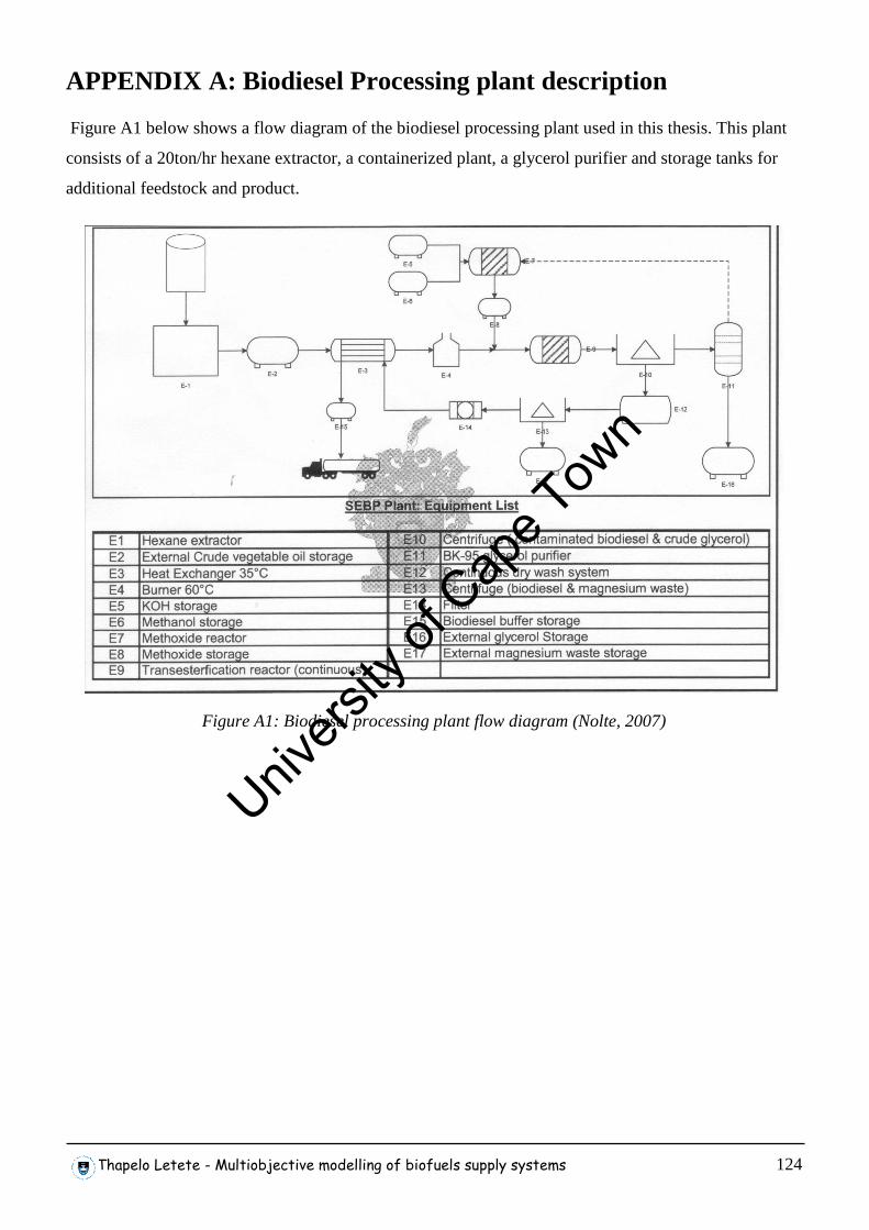
Thapelo Letete - Multiobjective modelling of biofuels supply systems 124
APPENDIX A: Biodiesel Processing plant description
Figure A1 below shows a flow diagram of the biodiesel processing plant used in this thesis. This plant
consists of a 20ton/hr hexane extractor, a containerized plant, a glycerol purifier and storage tanks for
additional feedstock and product.
Figure A1: Biodiesel processing plant flow diagram (Nolte, 2007)
Univers
ity of
Cap
e Tow
n
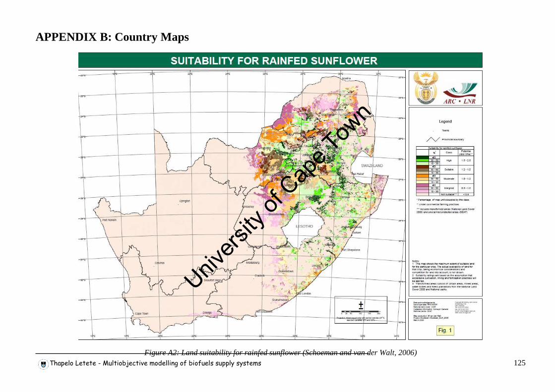
Thapelo Letete - Multiobjective modelling of biofuels supply systems 125
APPENDIX B: Country Maps
Figure A2: Land suitability for rainfed sunflower (Schoeman and van der Walt, 2006) Univ
ersity
of C
ape T
own
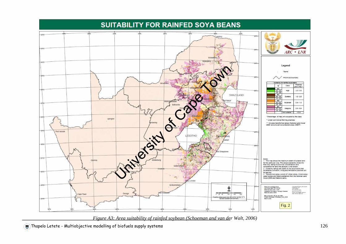
Thapelo Letete - Multiobjective modelling of biofuels supply systems 126
Figure A3: Area suitability of rainfed soybean (Schoeman and van der Walt, 2006) Univ
ersity
of C
ape T
own
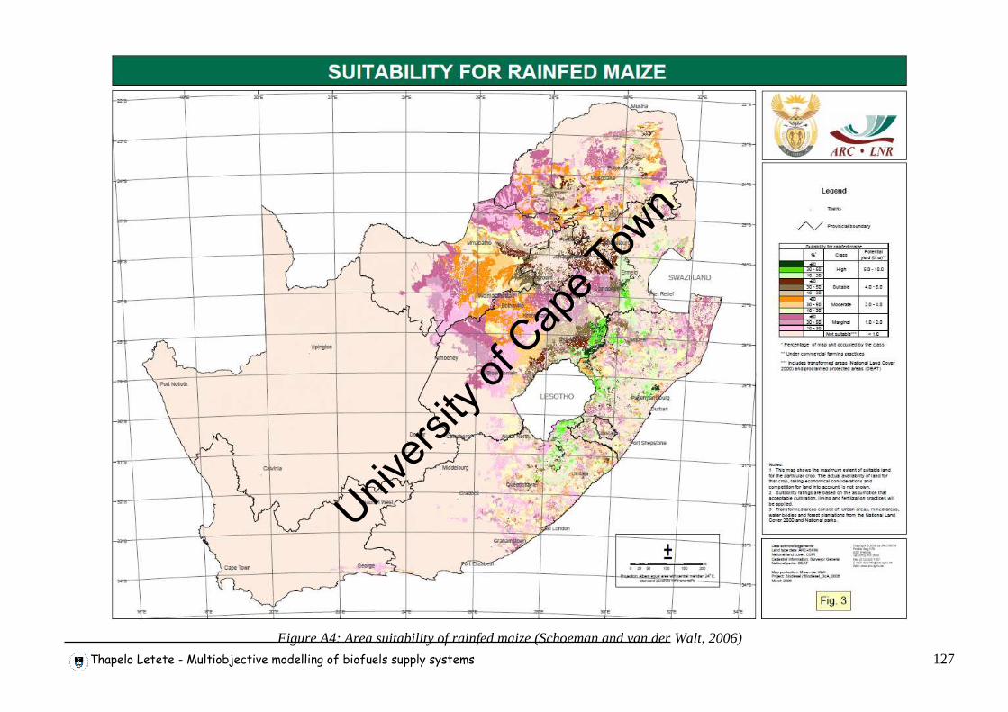
Thapelo Letete - Multiobjective modelling of biofuels supply systems 127
Figure A4: Area suitability of rainfed maize (Schoeman and van der Walt, 2006) Univ
ersity
of C
ape T
own
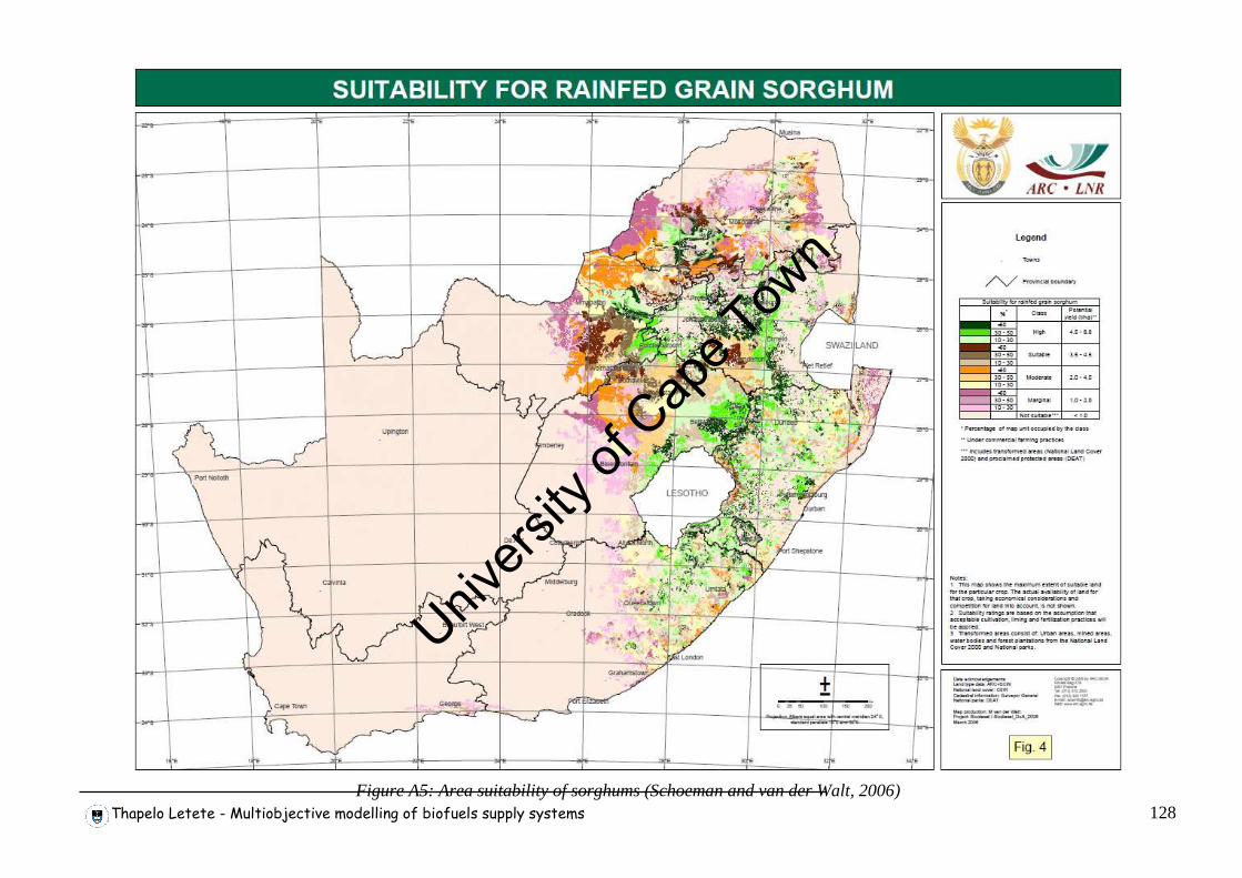
Thapelo Letete - Multiobjective modelling of biofuels supply systems 128
Figure A5: Area suitability of sorghums (Schoeman and van der Walt, 2006) Univ
ersity
of C
ape T
own
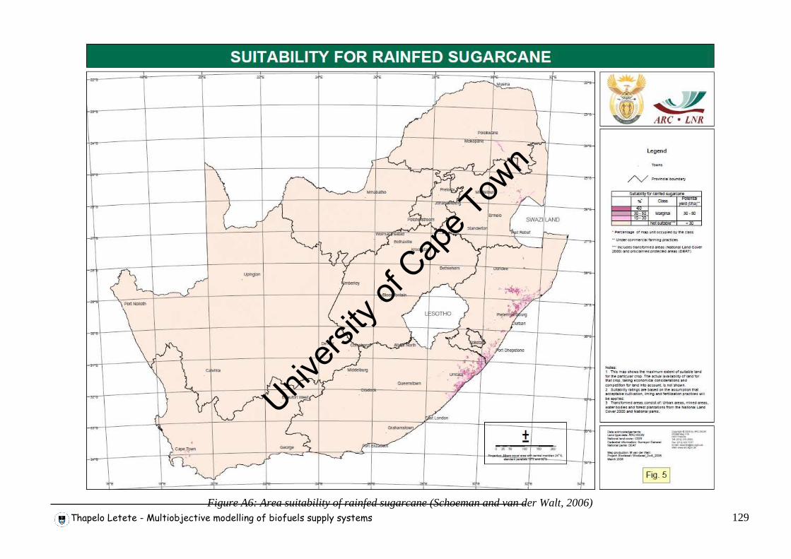
Thapelo Letete - Multiobjective modelling of biofuels supply systems 129
Figure A6: Area suitability of rainfed sugarcane (Schoeman and van der Walt, 2006) Univ
ersity
of C
ape T
own
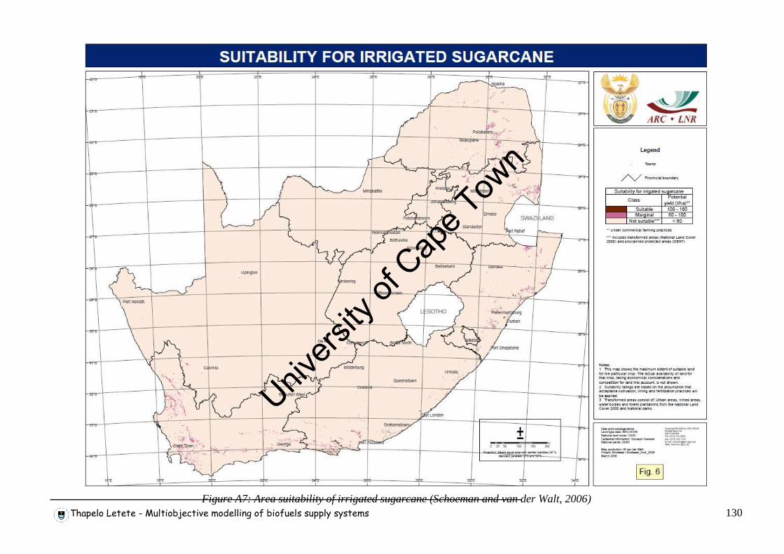
Thapelo Letete - Multiobjective modelling of biofuels supply systems 130
Figure A7: Area suitability of irrigated sugarcane (Schoeman and van der Walt, 2006) Univ
ersity
of C
ape T
own
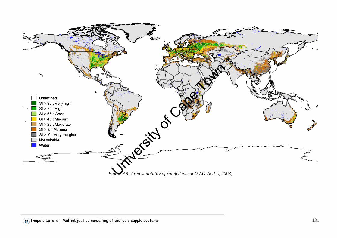
Thapelo Letete - Multiobjective modelling of biofuels supply systems 131
Figure A8: Area suitability of rainfed wheat (FAO-AGLL, 2003)
Univers
ity of
Cap
e Tow
n
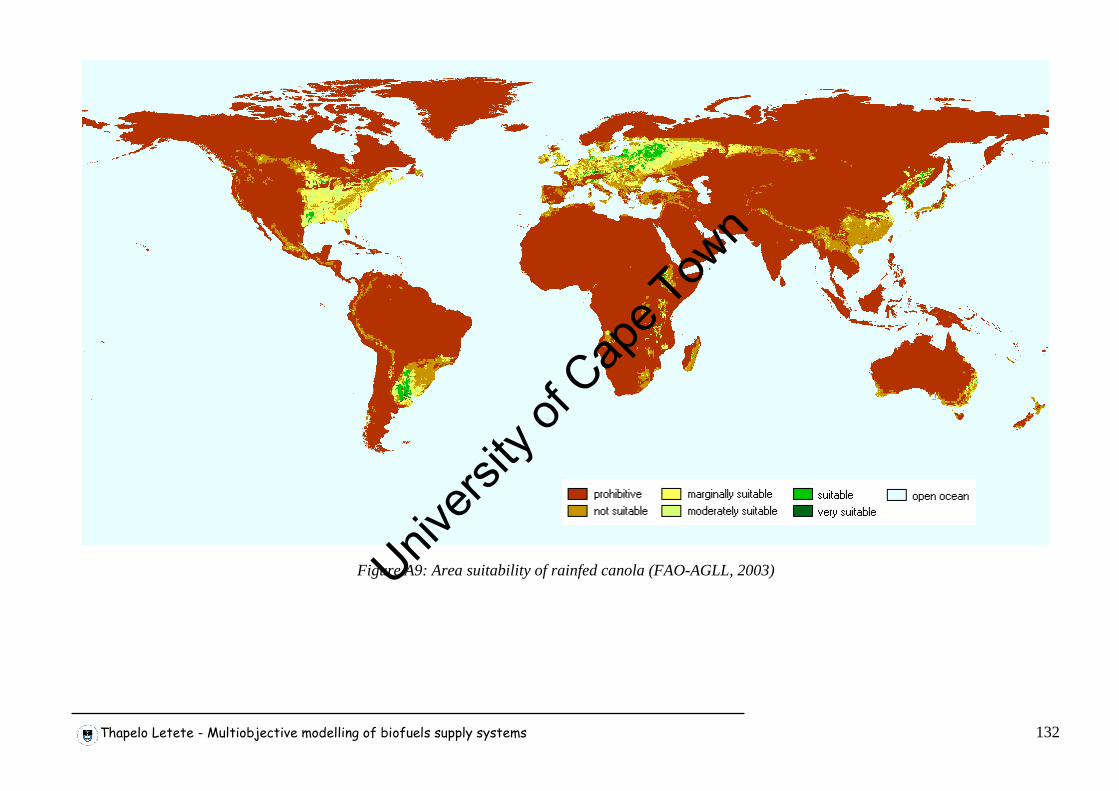
Thapelo Letete - Multiobjective modelling of biofuels supply systems 132
Figure A9: Area suitability of rainfed canola (FAO-AGLL, 2003)
Univ
ersity
of C
ape T
own
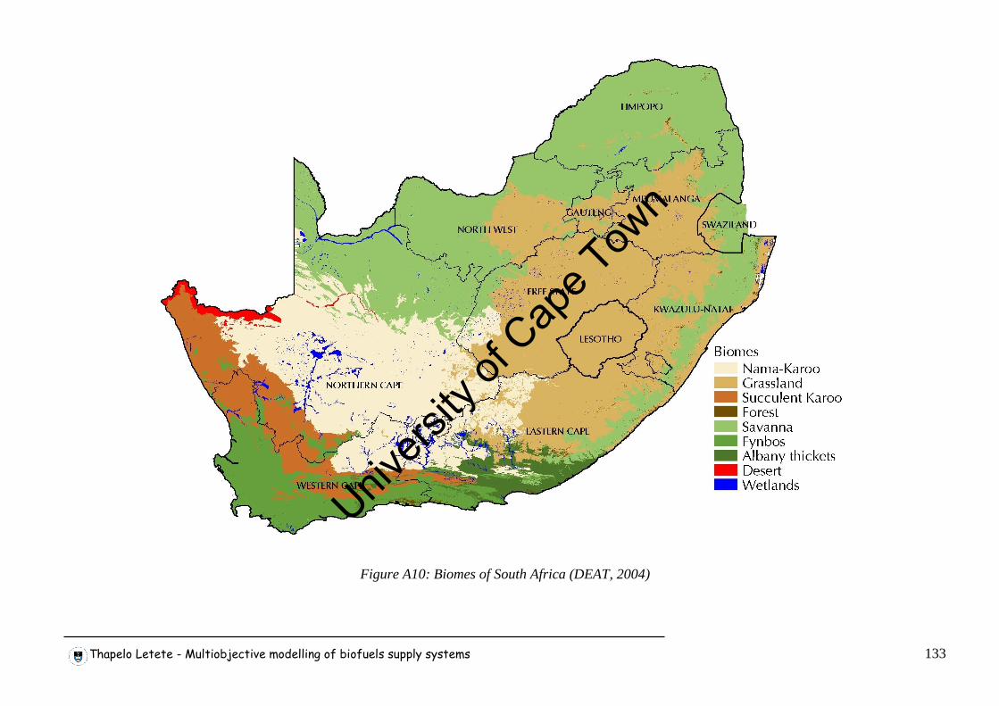
Thapelo Letete - Multiobjective modelling of biofuels supply systems 133
Figure A10: Biomes of South Africa (DEAT, 2004)
Univ
ersity
of C
ape T
own
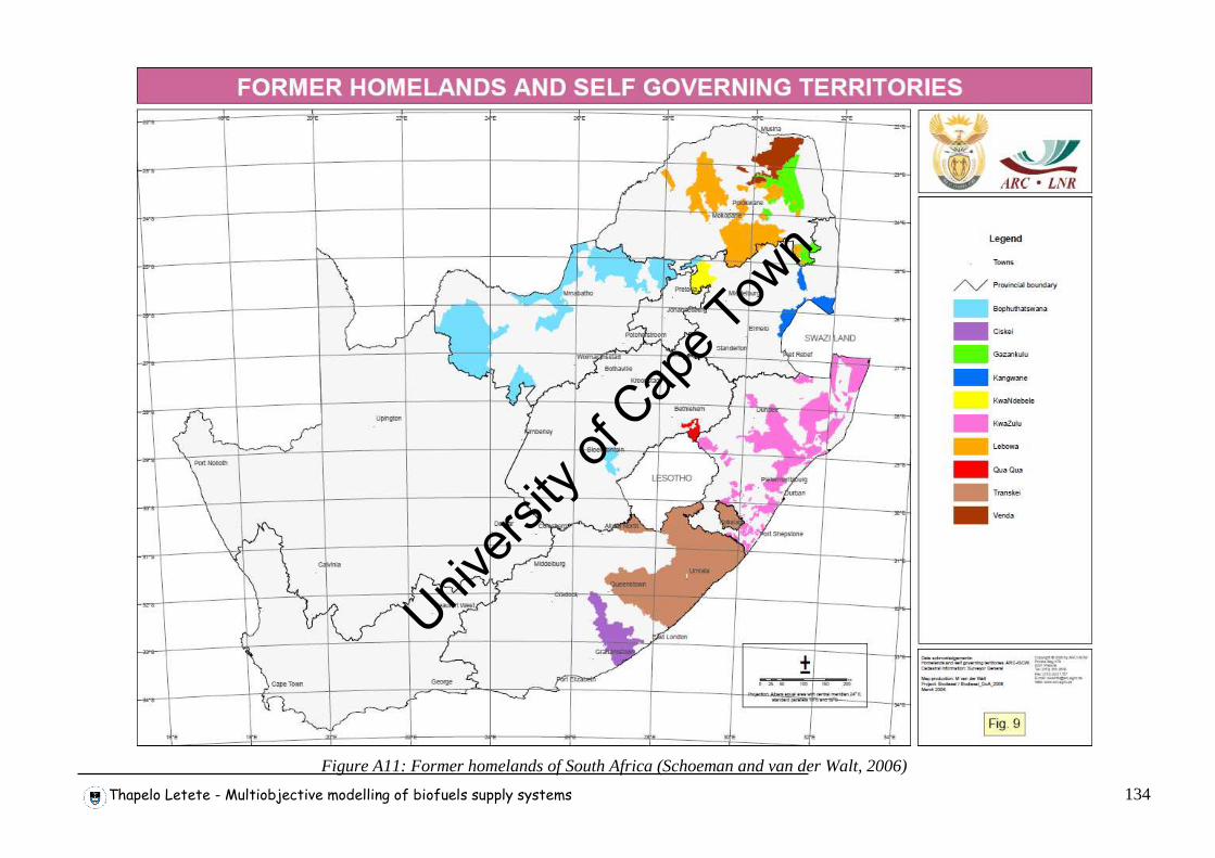
Thapelo Letete - Multiobjective modelling of biofuels supply systems 134
Figure A11: Former homelands of South Africa (Schoeman and van der Walt, 2006)Univ
ersity
of C
ape T
own
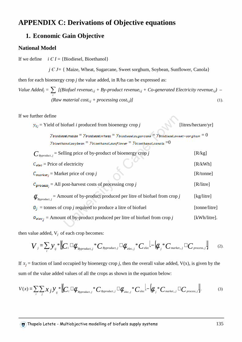
Thapelo Letete - Multiobjective modelling of biofuels supply systems 135
APPENDIX C: Derivations of Objective equations
1. Economic Gain Objective
National Model
If we define i Є I = {Biodiesel, Bioethanol}
j Є J= { Maize, Wheat, Sugarcane, Sweet sorghum, Soybean, Sunflower, Canola}
then for each bioenergy crop j the value added, in R/ha can be expressed as:
Value Addedj = ∑i
[(Biofuel revenuei,j + By-product revenuei,j + Co-generated Electricity revenuei,j) –
(Raw material costi,j + processing costi,j)] (1).
If we further define
= Yield of biofuel i produced from bioenergy crop j [litres/hectare/yr]
= = = = 0
= = =0
C jByproduct,= Selling price of by-product of bioenergy crop j [R/kg]
= Price of electricity [R/kWh]
= Market price of crop j [R/tonne]
= All post-harvest costs of processing crop j [R/litre]
φjByproduct,= Amount of by-product produced per litre of biofuel from crop j [kg/litre]
= tonnes of crop j required to produce a litre of biofuel [tonne/litre]
= Amount of by-product produced per litre of biofuel from crop j [kWh/litre].
then value added, Vj of each crop becomes:
( ) ( )[ ]∑ +−++=i
jprocessjmarketjelecjelecjByproductjByproductiijj CCCCCyV ,,,,,,**** φφφ (2).
If = fraction of land occupied by bioenergy crop j, then the overall value added, V(x), is given by the
sum of the value added values of all the crops as shown in the equation below:
( ) ( )[ ]∑∑ +−++=i j
jprocessjmarketjelecjelecjByproductjByproductiijCCCCCyx jxV
,,,,,,****)( φφφ . (3)
Univers
ity of
Cap
e Tow
n
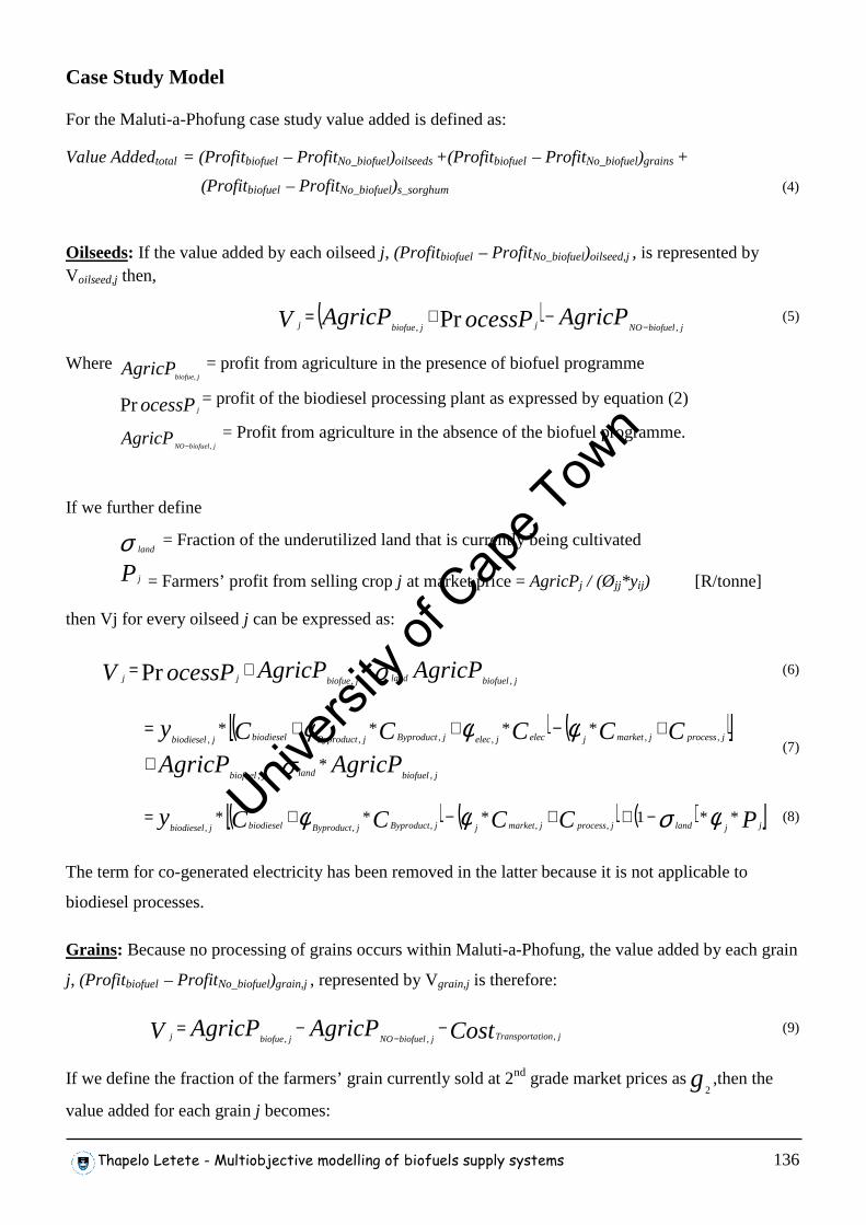
Thapelo Letete - Multiobjective modelling of biofuels supply systems 136
Case Study Model
For the Maluti-a-Phofung case study value added is defined as:
Value Addedtotal = (Profitbiofuel – ProfitNo_biofuel)oilseeds +(Profitbiofuel – ProfitNo_biofuel)grains +
(Profitbiofuel – ProfitNo_biofuel)s_sorghum (4)
Oilseeds: If the value added by each oilseed j, (Profitbiofuel – ProfitNo_biofuel)oilseed,j , is represented by Voilseed,j then,
( ) AgricPocessPAgricPV jbiofuelNOjjbiofuej ,, Pr −−+= (5)
Where AgricPjbiofue,
= profit from agriculture in the presence of biofuel programme
ocessPjPr = profit of the biodiesel processing plant as expressed by equation (2)
AgricPjbiofuelNO ,− = Profit from agriculture in the absence of the biofuel programme.
If we further define
σ land = Fraction of the underutilized land that is currently being cultivated
Pj = Farmers’ profit from selling crop j at market price = AgricPj / (Øjj*y ij) [R/tonne]
then Vj for every oilseed j can be expressed as:
AgricPAgricPocessPV jbiofuellandjbiofuejj ,,Pr σ−+= (6)
( ) ( )[ ]AgricPAgricP
CCCCCy
jbiofuellandjbiofuel
jprocessjmarketjelecjelecjByproductjByproductbiodieseljbiodiesel
,,
,,,,,,
*
****
σφφφ
−+
+−++= (7)
( ) ( ) ( )[ ]PCCCCy jjlandjprocessjmarketjjByproductjByproductbiodieseljbiodiesel**1***
,,,,,φσφφ −++−+= (8)
The term for co-generated electricity has been removed in the latter because it is not applicable to
biodiesel processes.
Grains: Because no processing of grains occurs within Maluti-a-Phofung, the value added by each grain
j, (Profitbiofuel – ProfitNo_biofuel)grain,j , represented by Vgrain,j is therefore:
CostAgricPAgricPV jtionTransportajbiofuelNOjbiofuej ,,,−−=
− (9)
If we define the fraction of the farmers’ grain currently sold at 2nd grade market prices asg2,then the
value added for each grain j becomes:
Univers
ity of
Cap
e Tow
n
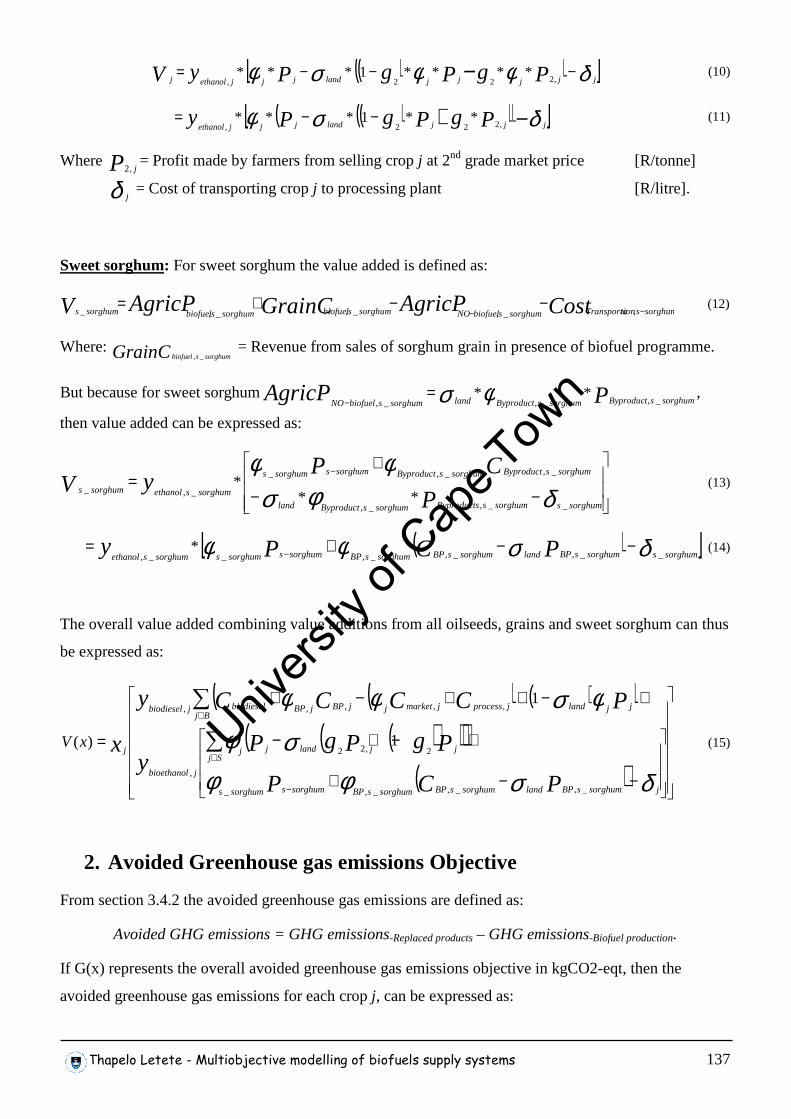
Thapelo Letete - Multiobjective modelling of biofuels supply systems 137
( )( )[ ]δφφσφ jjjjjlandjjjethanolj PgPgPyV −−−= − ,222,****1*** (10)
( )( )( )[ ]δσφ −+−−=jjjlandjjjethanol PgPgPy ,222,
**1*** (11)
Where P j,2= Profit made by farmers from selling crop j at 2nd grade market price [R/tonne]
δ j = Cost of transporting crop j to processing plant [R/litre].
Sweet sorghum: For sweet sorghum the value added is defined as:
CostAgricPGrainCAgricPV sorghumstionTransportasorghumsbiofuelNOsorghumsbiofuelsorghumsbiofuelsorghums −−−−+=
,_,_,_,_ (12)
Where: GrainC sorghumsbiofuel _, = Revenue from sales of sorghum grain in presence of biofuel programme.
But because for sweet sorghum PAgricP sorghumsByproductsorghumsByproductlandsorghumsbiofuelNO _,_,_,**φσ=
−,
then value added can be expressed as:
−−
+=
−
δφσφφ
sorghumssorghumsByproductssorghumsByproductland
sorghumsByproductsorghumsByproductsorghumssorghums
sorghumsethanolsorghums
P
CPyV
__,_,
_,_,_
_,_**
* (13)
( )[ ]δσφφ sorghumssorghumsBPlandsorghumsBPsorghumsBPsorghumssorghumssorghumsethanol PCPy __,_,_,__,* −−+= − (14)
The overall value added combining value additions from all oilseeds, grains and sweet sorghum can thus
be expressed as:
( ) ( )( )( )( )( )
( )
−−+
+−+−
+−++−+
=
−
∈
∈
∑
∑
δσφφσφ
φσφφ
jsorghumsBPlandsorghumsBPsorghumsBPsorghumssorghums
Sjjjlandjj
jbioethanol
BjjjlandjprocessjmarketjjBPjBPbiodieseljbiodiesel
j
PCP
PgPgPy
PCCCCy
xxV
_,_,_,_
2,22
,
,,,,,
1
1
)( (15)
2. Avoided Greenhouse gas emissions Objective
From section 3.4.2 the avoided greenhouse gas emissions are defined as:
Avoided GHG emissions = GHG emissions-Replaced products – GHG emissions-Biofuel production.
If G(x) represents the overall avoided greenhouse gas emissions objective in kgCO2-eqt, then the
avoided greenhouse gas emissions for each crop j, can be expressed as:
Univers
ity of
Cap
e Tow
n
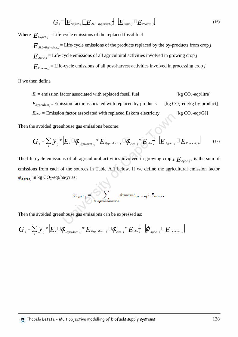
Thapelo Letete - Multiobjective modelling of biofuels supply systems 138
[ ] [ ]EEEEG jocessjAgricjByproductALLjbiofuelj ,Pr,,,+−= + − (16)
Where E jbiofuel,= Life-cycle emissions of the replaced fossil fuel
E jByproductALL ,− = Life-cycle emissions of the products replaced by the by-products from crop j
E jAgric,= Life-cycle emissions of all agricultural activities involved in growing crop j
E jocess,Pr= Life-cycle emissions of all post-harvest activities involved in processing crop j
If we then define
Ei = emission factor associated with replaced fossil fuel [kg CO2-eqt/litre]
EByproduct,j = Emission factor associated with replaced by-products [kg CO2-eqt/kg by-product]
Eelec = Emission factor associated with replaced Eskom electricity [kg CO2-eqt/GJ]
Then the avoided greenhouse gas emissions become:
[ ] [ ]EEEEEyG jocessjAgrici
elecjelecjByproductjByproductiijj ,Pr,,,,*** +−++=∑ φφ (17)
The life-cycle emissions of all agricultural activities involved in growing crop j,E jAgric,, is the sum of
emissions from each of the sources in Table A.1 below. If we define the agricultural emission factor
in kg CO2-eqt/ha/yr as:
Then the avoided greenhouse gas emissions can be expressed as:
[ ] [ ]EEEEyG jocessjagrici
elecjelecjByproductjByproductiijj ,Pr,,,,*** +−++= ∑ ϕφφ
Univers
ity of
Cap
e Tow
n
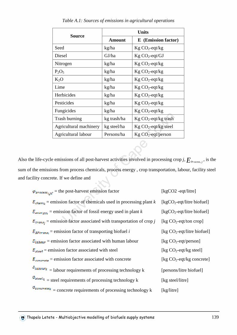
Thapelo Letete - Multiobjective modelling of biofuels supply systems 139
Table A.1: Sources of emissions in agricultural operations
Units Source
Amount E (Emission factor)
Seed kg/ha Kg CO2-eqt/kg
Diesel GJ/ha Kg CO2-eqt/GJ
Nitrogen kg/ha Kg CO2-eqt/kg
P2O5 kg/ha Kg CO2-eqt/kg
K2O kg/ha Kg CO2-eqt/kg
Lime kg/ha Kg CO2-eqt/kg
Herbicides kg/ha Kg CO2-eqt/kg
Pesticides kg/ha Kg CO2-eqt/kg
Fungicides kg/ha Kg CO2-eqt/kg
Trash burning kg trash/ha Kg CO2-eqt/kg trash
Agricultural machinery kg steel/ha Kg CO2-eqt/kg steel
Agricultural labour Persons/ha Kg CO2-eqt/person
Also the life-cycle emissions of all post-harvest activities involved in processing crop j,E jocess,Pr, is the
sum of the emissions from process chemicals, process energy , crop transportation, labour, facility steel
and facility concrete. If we define and
, = the post-harvest emission factor [kgCO2 -eqt/litre]
= emission factor of chemicals used in processing plant k [kgCO2-eqt/litre biofuel]
= emission factor of fossil energy used in plant k [kgCO2-eqt/litre biofuel]
= emission factor associated with transportation of crop j [kg CO2-eqt/ton crop]
= emission factor of transporting biofuel i [kg CO2-eqt/litre biofuel]
= emission factor associated with human labour [kg CO2-eqt/person]
= emission factor associated with steel [kg CO2-eqt/kg steel]
= emission factor associated with concrete [kg CO2-eqt/kg concrete]
= labour requirements of processing technology k [persons/litre biofuel]
= steel requirements of processing technology k [kg steel/litre]
= concrete requirements of processing technology k [kg/litre]
Univers
ity of
Cap
e Tow
n
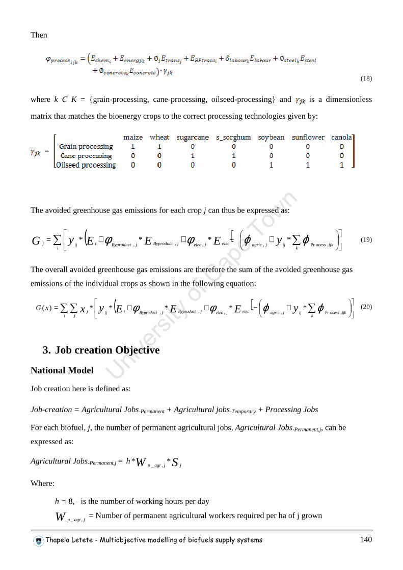
Thapelo Letete - Multiobjective modelling of biofuels supply systems 140
Then
(18)
where k Є K = {grain-processing, cane-processing, oilseed-processing} and is a dimensionless
matrix that matches the bioenergy crops to the correct processing technologies given by:
=
The avoided greenhouse gas emissions for each crop j can thus be expressed as:
( )∑ ∑
+−++=i k
ijkocessijjagricelecjelecjByproductjByproductiijj yEEEyG ϕϕφφ,Pr,,,,
**** (19)
The overall avoided greenhouse gas emissions are therefore the sum of the avoided greenhouse gas
emissions of the individual crops as shown in the following equation:
( )∑∑ ∑
+−++=i j k
ijkocessijjagricelecjelecjByproductjByproductiijj yEEEyxxG ϕϕφφ,Pr,,,,
*****)( (20)
3. Job creation Objective
National Model
Job creation here is defined as:
Job-creation = Agricultural Jobs-Permanent + Agricultural jobs-Temporary + Processing Jobs
For each biofuel, j, the number of permanent agricultural jobs, Agricultural Jobs-Permanent,j, can be
expressed as:
Agricultural Jobs-Permanent,j = SW jjagrph **
,_
Where:
h = 8, is the number of working hours per day
W jagrp ,_ = Number of permanent agricultural workers required per ha of j grown
Univers
ity of
Cap
e Tow
n
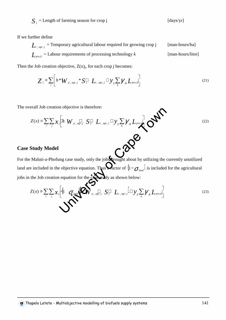
Thapelo Letete - Multiobjective modelling of biofuels supply systems 141
Sj = Length of farming season for crop j [days/yr]
If we further define
L jagrt ,_ = Temporary agricultural labour required for growing crop j [man-hours/ha]
L kpro, = Labour requirements of processing technology k [man-hours/litre]
Then the Job creation objective, Z(x)j, for each crop j becomes:
∑ ∑
++=i k
kprojkijjagrtjjagrpj LyLSWZ h,,_,_
** γ (21)
The overall Job creation objective is therefore:
∑∑ ∑
++⋅⋅=i j k
kprojkijjagrtjjagrpj LyLSWx hxZ,,_,_
)( γ (22)
Case Study Model
For the Maluti-a-Phofung case study, only the jobs brought about by utilizing the currently unutilized
land are included in the objective equation. Thus a factor of ( )σ land−1 is included for the agricultural
jobs in the Job creation equation for the case study as shown below:
( )( )∑∑ ∑
++⋅⋅−=i j k
kprojkijjagrtjjagrplandj LyLSWx hxZ,,_,_
1)( γσ (23)
Univers
ity of
Cap
e Tow
n
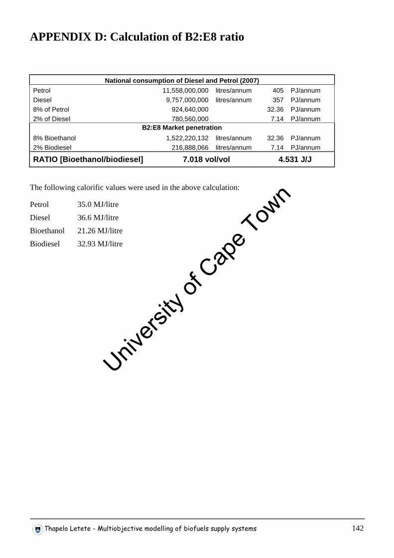
Thapelo Letete - Multiobjective modelling of biofuels supply systems 142
APPENDIX D: Calculation of B2:E8 ratio
National consumption of Diesel and Petrol (2007)
Petrol 11,558,000,000 litres/annum 405 PJ/annum Diesel 9,757,000,000 litres/annum 357 PJ/annum 8% of Petrol 924,640,000 32.36 PJ/annum 2% of Diesel 780,560,000 7.14 PJ/annum
B2:E8 Market penetration
8% Bioethanol 1,522,220,132 litres/annum 32.36 PJ/annum 2% Biodiesel 216,888,066 litres/annum 7.14 PJ/annum
RATIO [Bioethanol/biodiesel] 7.018 vol/vol 4.531 J/J
The following calorific values were used in the above calculation:
Petrol 35.0 MJ/litre
Diesel 36.6 MJ/litre
Bioethanol 21.26 MJ/litre
Biodiesel 32.93 MJ/litre
Univers
ity of
Cap
e Tow
n
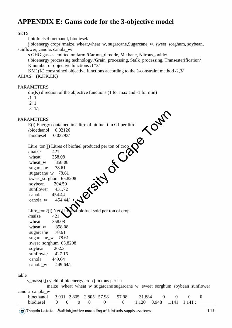
Thapelo Letete - Multiobjective modelling of biofuels supply systems 143
APPENDIX E: Gams code for the 3-objective model
SETS i biofuels /bioethanol, biodiesel/ j bioenergy crops /maize, wheat,wheat_w, sugarcane,Sugarcane_w, sweet_sorghum, soybean, sunflower, canola, canola_w/ s GHG gasses emitted on farm /Carbon_dioxide, Methane, Nitrous_oxide/ t bioenergy processing technology /Grain_processing, Stalk_processing, Transesterification/ K number of objective functions /1*3/ KM1(K) constrained objective functions according to the å-constraint method /2,3/ ALIAS (K,KK,LK) PARAMETERS dir(K) direction of the objective functions (1 for max and -1 for min) /1 1 2 1 3 1/; PARAMETERS E(i) Energy contained in a litre of biofuel i in GJ per litre /bioethanol 0.02126 biodiesel 0.03293/ Litre_ton(j) Litres of biofuel produced per ton of crop /maize 421 wheat 358.08 wheat_w 358.08 sugarcane 78.61 sugarcane_w 78.61 sweet_sorghum 65.8208 soybean 204.50 sunflower 431.72 canola 454.44 canola_w 454.44/ Litre_ton2(j) Net Litres of biofuel sold per ton of crop /maize 421 wheat 358.08 wheat_w 358.08 sugarcane 78.61 sugarcane_w 78.61 sweet_sorghum 65.8208 soybean 202.3 sunflower 427.16 canola 449.64 canola_w 449.64/; table y_mass(i,j) yield of bioenergy crop j in tons per ha maize wheat wheat_w sugarcane sugarcane_w sweet_sorghum soybean sunflower canola canola_w bioethanol 3.031 2.805 2.805 57.98 57.98 31.884 0 0 0 0 biodiesel 0 0 0 0 0 0 1.120 0.948 1.141 1.141 ;
Univers
ity of
Cap
e Tow
n
Thapelo Letete - Multiobjective modelling of biofuels supply systems 144
parameter y(i,j) yield of bioenergy crop j in litres per ha; y(i,j)= Litre_ton(j) * y_mass(i,j); parameters E_dummy(i) dummy parameter for bioethanol /bioethanol 1 biodiesel 0/ D_dummy(i) dummy parameter for biodiesel /bioethanol 0 biodiesel 1/ Maize_(j) dummy parameter for maize /maize 1 wheat 0 wheat_w 0 sugarcane 0 sugarcane_w 0 sweet_sorghum 0 soybean 0 sunflower 0 canola 0 canola_w 0/ Wheat_(j) dummy parameter for wheat /maize 0 wheat 1 wheat_w 0 sugarcane 0 sugarcane_w 0 sweet_sorghum 0 soybean 0 sunflower 0 canola 0 canola_w 0/ Wheat_w_(j) dummy parameter for wheat_w /maize 0 wheat 0 wheat_w 1 sugarcane 0 sugarcane_w 0 sweet_sorghum 0 soybean 0 sunflower 0 canola 0 canola_w 0/ sugarcane_(j) dummy parameter for sugarcane /maize 0 wheat 0 wheat_w 0 sugarcane 1 sugarcane_w 0 sweet_sorghum 0 soybean 0
Univers
ity of
Cap
e Tow
n
Thapelo Letete - Multiobjective modelling of biofuels supply systems 145
sunflower 0 canola 0 canola_w 0/ sugarcane_w_(j) dummy parameter for sugarcane_w /maize 0 wheat 0 wheat_w 0 sugarcane 0 sugarcane_w 1 sweet_sorghum 0 soybean 0 sunflower 0 canola 0 canola_w 0/ Sweetsorghum_(j) dummy parameter for sweet sorghum /maize 0 wheat 0 wheat_w 0 sugarcane 0 sugarcane_w 0 sweet_sorghum 1 soybean 0 sunflower 0 canola 0 canola_w 0/ soybean_(j) dummy parameter for soybean /maize 0 wheat 0 wheat_w 0 sugarcane 0 sugarcane_w 0 sweet_sorghum 0 soybean 1 sunflower 0 canola 0 canola_w 0/ sunflower_(j) dummy parameter for sunflower /maize 0 wheat 0 wheat_w 0 sugarcane 0 sugarcane_w 0 sweet_sorghum 0 soybean 0 sunflower 1 canola 0 canola_w 0/ Canola_(j) dummy parameter for canola /maize 0 wheat 0 wheat_w 0 sugarcane 0 sugarcane_w 0
Univers
ity of
Cap
e Tow
n
Thapelo Letete - Multiobjective modelling of biofuels supply systems 146
sweet_sorghum 0 soybean 0 sunflower 0 canola 1 canola_w 0/ Canola_w_(j) dummy parameter for canola_w /maize 0 wheat 0 wheat_w 0 sugarcane 0 sugarcane_w 0 sweet_sorghum 0 soybean 0 sunflower 0 canola 0 canola_w 1/; parameters Amt_BP_mass(j) kg of by-product per ton of energy crop (grain for sweet sorghum) /maize 318.316 wheat 430.694 wheat_w 430.694 sugarcane 0 sugarcane_w 0 sweet_sorghum 47.193 soybean 779 sunflower 620 canola 600 canola_w 600/ Amt_Elec(j) quantity of excess electricity sold in kWh per litre /maize 0 wheat 0 wheat_w 0 sugarcane 0.21 sugarcane_w 0.21 sweet_sorghum 0.1572 soybean 0 sunflower 0 canola 0 canola_w 0/ C_p_market(j) Market(purchase)price of energy crop j in ZAR per tonne /maize 1805 wheat 3706 wheat_w 3706 sugarcane 207.54 sugarcane_w 207.54 sweet_sorghum 207.54 soybean 4550 sunflower 4935 canola 3500 canola_w 3500/
Univers
ity of
Cap
e Tow
n
Thapelo Letete - Multiobjective modelling of biofuels supply systems 147
C_process(j) Processing cost of energy crop j in ZAR per litre /maize 3.02 wheat 3.11 wheat_w 3.11 sugarcane 2.42 sugarcane_w 2.42 sweet_sorghum 3.48 soybean 3.86 sunflower 2.74 canola 2.67 canola_w 2.67/ C_BP(j) Selling price of by-product from crop j in ZAR per kg by-product /maize 2.78 wheat 2.69 wheat_w 2.69 sugarcane 0 sugarcane_w 0 sweet_sorghum 1.534 soybean 4.09 sunflower 2.95 canola 2.43 canola_w 2.43/ SP(i) Selling price of biofuel i in ZAR per litre(verify these values one last time) /bioethanol 7.01 biodiesel 6.92/ RHS(K) right hand side of the constrained obj.functions in e-constraint MAXOBJ(K) maximum value from the payoff table MINOBJ(K) minimum value from the payoff table w(k) indicator parameters for the objective functions PAYOFF(K,KK) payoff table entries; * necessary initial values for the parameters MAXOBJ(K) = 1; MINOBJ(K) = 0; PAYOFF(K,KK) = 0; parameters *Avoided CO2 emission parameters Amt_DSL(j) kg of Diesel used per ha in agricultural activities of j /maize 71.75 wheat 64.5 wheat_w 64.5 sugarcane 74.26 sugarcane_w 74.26 sweet_sorghum 155.119 soybean 65.47 sunflower 62.4 canola 62.5 canola_w 62.5/
Univers
ity of
Cap
e Tow
n
Thapelo Letete - Multiobjective modelling of biofuels supply systems 148
Amt_N2(j) kg of N2 used per ha of j grown /maize 52.3 wheat 30 wheat_w 30 sugarcane 92 sugarcane_w 92 sweet_sorghum 120 soybean 2.8 sunflower 12.8 canola 57.5 canola_w 57.5/ Amt_P2O5(j) kg of P2O5 used per ha of j grown /maize 28.5 wheat 40 wheat_w 40 sugarcane 57 sugarcane_w 57 sweet_sorghum 40 soybean 10 sunflower 17.9 canola 68.8 canola_w 68.8/ Amt_K2O(j) kg of K2O used per ha of j grown /maize 5.7 wheat 4 wheat_w 4 sugarcane 133 sugarcane_w 133 sweet_sorghum 40 soybean 3.2 sunflower 1.7 canola 65.2 canola_w 65.2/ Amt_Herb(j) kg of Herbicide used per ha of j grown /maize 2.2 wheat 4.935 wheat_w 4.935 sugarcane 2.2 sugarcane_w 2.2 sweet_sorghum 3.0 soybean 0 sunflower 2.5 canola 1.02 canola_w 1.02/ Amt_Ins(j) kg of Insecticide used per ha of j grown /maize 0.08 wheat 1.07 wheat_w 1.07
Univers
ity of
Cap
e Tow
n
Thapelo Letete - Multiobjective modelling of biofuels supply systems 149
sugarcane 0.16 sugarcane_w 0.16 sweet_sorghum 9.0 soybean 1.2 sunflower 0 canola 0.036 canola_w 0.036/ Amt_Fungi(j) kg of Fungicide used per ha of j grown /maize 0.0 wheat 2.0 wheat_w 2.0 sugarcane 0.0 sugarcane_w 0.0 sweet_sorghum 0.0 soybean 0.0 sunflower 0.0 canola 0.0 canola_w 0.0/ Amt_Trash(j) kg of trash burned per ha of j grown /maize 0 wheat 0 wheat_w 0 sugarcane 5705 sugarcane_w 5705 sweet_sorghum 0 soybean 0 sunflower 0 canola 0 canola_w 0/ Amt_Agrsteel(j) kg of steel in agricultural implements per ha of j grown /maize 23.022 wheat 23.022 wheat_w 23.022 sugarcane 33.462 sugarcane_w 33.462 sweet_sorghum 23.02 soybean 20.8 sunflower 20.8 canola 20.8 canola_w 20.8/ Agr_labor(j) Agricultural labour requirements per ha of j grown /maize 0.00848 wheat 0.00848 wheat_w 0.00848 sugarcane 0.0767 sugarcane_w 0.0767 sweet_sorghum 0.00848 soybean 0.00848 sunflower 0.00848
Univers
ity of
Cap
e Tow
n
Thapelo Letete - Multiobjective modelling of biofuels supply systems 150
canola 0.00848 canola_w 0.00848/ Amt_Seed(j) kg of seed required per ha of j grown /maize 12.5 wheat 120 wheat_w 120 sugarcane 1 sugarcane_w 1 sweet_sorghum 7.250 soybean 76.1 sunflower 3.5 canola 4.5 canola_w 4.5/ Em_fuel_eqt(i) CO2-eqt emissions of biofuels per GJ of fuel i burnt /bioethanol 81.8 biodiesel 88.26/ Em_BP(j) CO2-eqt emissions of by-product of j per litre biofuel sold /maize 0.812 wheat 1.438 wheat_w 1.438 sugarcane 0.202 sugarcane_w 0.202 sweet_sorghum 0.606 soybean 3.274 sunflower 1.238 canola 1.067 canola_w 1.067/ Em_Seed(j) CO2-eqt emissions per kg seed of j used /maize 3.85 wheat 0.4033 wheat_w 0.4033 sugarcane 27.07 sugarcane_w 27.07 sweet_sorghum 3.15 soybean 0.92 sunflower 2.77 canola 0.32 canola_w 0.32/ *Technology dependant parameters Em_chem(t) CO2-eqt emissions of chemicals used in technology t per litre of biofuel (grain assumed equal to stalk) /Grain_processing 0.023 Stalk_processing 0.023 Transesterification 0.067/ Em_crop_trans(j) CO2-eqt emissions from transporting a tonne of crop j /maize 26.77 wheat 21.97
Univers
ity of
Cap
e Tow
n
Thapelo Letete - Multiobjective modelling of biofuels supply systems 151
wheat_w 21.97 sugarcane 4.13 sugarcane_w 4.13 sweet_sorghum 77.21 soybean 10.17 sunflower 10.17 canola 10.17 canola_w 10.17/ Em_bf_trans(i) CO2-eqt emissions from transporting a litre of biofuel i /Bioethanol 0.0276 Biodiesel 0.0276/ Tech_labor(t) Post agriculture labour requirements in persons per litre of biofuel /Grain_processing 0.00000042 Stalk_processing 0.00000154 Transesterification 0.00000302/ Amt_techsteel(t) kg of steel used in constructing processing plant t per litre /Grain_processing 0.00067 Stalk_processing 0.0015 Transesterification 0.0011/ Amt_concrete(t) kg of concrete used in constructing processing plant t per litre /Grain_processing 0.0062 Stalk_processing 0.0051 Transesterification 0.0088/; table Em_Energy(t,j) CO2-eqt emissions of FF Energy used in technology t per litre maize wheat wheat_w sugarcane sugarcane_w sweet_sorghum soybean sunflower canola canola_w Grain_processing 670.12 569.97 569.97 0 0 0 0 0 0 0 Stalk_processing 0 0 0 0 0 0 0 0 0 0 Transesterification 0 0 0 0 0 0 144.8 144.8 144.8 144.8; parameters Season(j) length of cropping season for crop j in days /maize 150 wheat 180 wheat_w 180 sugarcane 365 sugarcane_w 365 sweet_sorghum 150 soybean 150 sunflower 150 canola 180 canola_w 180 / Agr_labor_temp(j) Temporary labour required for harvesting crop j in man-hours per ha /maize 32.88
Univers
ity of
Cap
e Tow
n
Thapelo Letete - Multiobjective modelling of biofuels supply systems 152
wheat 0 wheat 0 sugarcane 121.0 sugarcane_w 121.0 sweet_sorghum 197.7 soybean 0 sunflower 0 canola 0 canola_w 0/ Tech_labor_MAP(t) Technology labour requirements in man-hours per litre /Grain_processing 0.00131 Stalk_processing 0.00556 Transesterification 0.00252/; table T_filter(t,j) Technology filter maize wheat wheat_w sugarcane sugarcane_w sweet_sorghum soybean sunflower canola canola_w Grain_processing 1 1 1 0 0 0 0 0 0 0 Stalk_processing 0 0 0 1 1 1 0 0 0 0 Transesterification 0 0 0 0 0 0 1 1 1 1; scalars Em_N2 CO2-eqt emissions per kg of N2 fertilizer /9.08/ Em_P2O5 CO2-eqt emissions per kg of P2O5 fertilizer /1.728/ Em_K2O CO2-eqt emissions per kg of K2O fertilizer /0.882/ Amt_lime kg of lime required per ha per annum (100-150) /194/ Em_lime CO2-eqt emission per kg of lime used /0.6494/ Em_Herb CO2-eqt emissions per kg of herbicide /32.43/ Em_Ins CO2-eqt emissions per kg of insecticide /37.55/ Em_Fungi CO2-eqt emissions per kg of fungicide /35.43/ Em_Trash CO2-eqt emissions per kg of trash burned /0.083/ Em_Steel CO2-eqt emissions per kg steel produced /11.17/ Em_labour National CO2-eqt emissions per capita /9.52/ Em_Concrete CO2-eqt emissions per kg concrete produced /0.82/ Em_DSL CO2-eqt emissions per GJ diesel fuel /88.26/ Diesel_Energy Energy of petroleum diesel in GJ per kg /0.04337/ C_elec cost of electricity in ZAR per kWh /0.2403/ h number of agricultural working hours per day /8/ BP_r fractional price increase of oilcake /1/ BP_r2 fractional price increase of sorghum grain /1/; parameter A_BP(j) Amount of by-product in kg of j per litre of biofuel; A_BP(j) = Amt_BP_mass(j)/Litre_ton2(j); parameter C_p(j) Total cost of producing biofuel from crop j in ZAR per litre; C_p(j) = C_p_market(j)/Litre_ton2(j)+ C_process(j); parameter A_DSL(j) GJ of diesel used per ha in agricultural activities of j; A_DSL(j) = Amt_DSL(j)*Diesel_Energy; parameter Em_AGR(j) Aggregated agricultural emissions factor of j; Em_AGR(j) = A_DSL(j)*Em_DSL+Amt_N2(j)*Em_N2+Amt_P2O5(j)*Em_P2O5+Amt_K2O(j)*Em_K2O+Amt_lim
Univers
ity of
Cap
e Tow
n
Thapelo Letete - Multiobjective modelling of biofuels supply systems 153
e*Em_lime+Amt_Herb(j)*Em_Herb+Amt_Ins(j)*Em_Ins+Amt_Fungi(j)*Em_Fungi+Amt_Trash(j)*Em_Trash+Amt_Agrsteel(j)*Em_Steel+Agr_labor(j)*Em_labour+Amt_Seed(j)*Em_Seed(j); parameter Em_PRO(i,j,t) Aggregated processing emissions factor of j; Em_PRO(i,j,t) = (Em_chem(t)+Em_Energy(t,j)/Litre_ton2(j)+Em_crop_trans(j)/Litre_ton2(j)+Em_bf_trans(i)+Tech_labor(t)*Em_labour+Amt_techsteel(t)*Em_Steel+Amt_concrete(t)*Em_Concrete)*T_filter(t,j); parameter coef_OBJ(K,i,j) Objective function coefficient; coef_OBJ('1',i,j) = y(i,j)*(SP(i)+A_BP(j)*C_BP(j)+Amt_Elec(j)*C_elec-C_p(j)); coef_OBJ('2',i,j) = y(i,j)*(E(i)*Em_fuel_eqt(i)+ Em_BP(j))-(Em_AGR(j)+sum((t),(y(i,j)*Em_PRO(i,j,t)))); coef_OBJ('3',i,j) = h*Agr_labor(j)*Season(j)+ Agr_labor_temp(j)+ y(i,j)*sum((t),(T_filter(t,j)*Tech_labor_MAP(t))); scalars r B2-E8 demand ratio of bioethanol vs biodiesel /4.5/ E_Ethanol Energy content of bioethanol in MJ per litre /21.26/ E_Diesel Energy content of biodiesel in MJ per litre /32.93/ land_w_c Western Cape land constraint constant /0.016/ land_o_c Rest of the country land constraint constant /0.984/ maize_c maize constraint constant /0.813/ wheat_c wheat constraint constant /0.61/ wheat_w_c wheat constraint constant /0.016/ sugar_c sugarcane constraint constant /0.045/ sugar_w_c sugarcane_w constraint constant /0.014/ sorghum_c sweet sorghum constraint constant /0.984/ soybean_c soybean constraint constant /0.573/ sunflower_c sunlower constraint constant /0.883/ canola_c canola constraint constant /0.315/ canola_w_c canola constraint constant /0.016/ * the following scalars are for the implementation of the e-constraint method g2, g3 counter for grid points per objective function 2 and 3 numg2 number of intervals per objective function 2 /5 / numg3 number of intervals per objective function 3 /5 / totcounter total counter of generated points jk counter used in the lexicographic optimization for the payoff table kopt auxiliary parameter ; POSITIVE VARIABLES SL(k) slack for max obj or surplus for min obj variables for e-constraint x(i,j) percentage of land used to grow crop j ; FREE VARIABLES Z(K) objective function variables OBJ auxiliary variable for the objective function during the construction of the payoff table A_OBJVAL auxiliary variable for the objective function of the å-constraint method ; EQUATIONS land_w western cape land availability constraint land_o other land availability constraint demand demand ratio constraint of diesel vs petrol science_E To assure that only sugar crops are grown for bioethanol
Univers
ity of
Cap
e Tow
n
Thapelo Letete - Multiobjective modelling of biofuels supply systems 154
science_D to assure that only oils are grown for biodiesel maize_suitability maize suitability constraint wheat_suitability wheat suitability constraint wheat_w_suitability wheat_w suitability constraint sugarcane_suitability sugarcane suitability constraint sugarcane_w_suitability sugarcane_w suitability constraint s_sorghum_suitability sweet sorghum suitability constraint soybean_suitability soybean suitability constraint sunflower_suitability sunflower suitability constraint canola_suitability canola suitability constraint canola_w_suitability canola suitability constraint OBJF(K) k-th objective function CON_OBJ(K) constrained objective functions AUGM_OBJ augmented objective function in order to avoid weakly efficient solutions ALLOBJ all the objective functions in one expression; land_w.. sum((i,j), x(i,j)*sugarcane_w_(j))+ sum((i,j), x(i,j)*canola_w_(j))+ sum((i,j), x(i,j)*wheat_w_(j)) =e= land_w_c; land_o.. sum((i,j), x(i,j)*maize_(j))+ sum((i,j), x(i,j)*wheat_(j))+ sum((i,j), x(i,j)*sugarcane_(j))+ sum((i,j), x(i,j)*sweetsorghum_(j))+ sum((i,j), x(i,j)*soybean_(j))+ sum((i,j), x(i,j)*sunflower_(j))+ sum((i,j), x(i,j)*canola_(j))=e= land_o_c; demand.. sum((i,j), x(i,j)*y(i,j)*E_dummy(i)) =e= r*sum((i,j), x(i,j)*y(i,j)*D_dummy(i)); science_E.. sum((i,j), x(i,j)*E_dummy(i)*soybean_(j))+ sum((i,j), x(i,j)*E_dummy(i)*sunflower_(j))+ sum((i,j), x(i,j)*E_dummy(i)*canola_(j))+sum((i,j), x(i,j)*E_dummy(i)*canola_w_(j)) =e= 0; science_D.. sum((i,j), x(i,j)*D_dummy(i)*maize_(j))+ sum((i,j), x(i,j)*D_dummy(i)*wheat_(j))+ sum((i,j), x(i,j)*D_dummy(i)*wheat_w_(j))+ sum((i,j), x(i,j)*D_dummy(i)*sugarcane_(j))+ sum((i,j), x(i,j)*D_dummy(i)*sugarcane_w_(j))+ sum((i,j), x(i,j)*D_dummy(i)*sweetsorghum_(j)) =e= 0 ; maize_suitability.. sum((i,j), x(i,j)*E_dummy(i)*maize_(j)) =l= maize_c; wheat_suitability.. sum((i,j), x(i,j)*E_dummy(i)*wheat_(j)) =l= wheat_c; wheat_w_suitability.. sum((i,j), x(i,j)*E_dummy(i)*wheat_w_(j)) =l= wheat_w_c; sugarcane_suitability.. sum((i,j), x(i,j)*E_dummy(i)*sugarcane_(j)) =l= sugar_c; sugarcane_w_suitability.. sum((i,j), x(i,j)*E_dummy(i)*sugarcane_w_(j)) =l= sugar_w_c; s_sorghum_suitability.. sum((i,j), x(i,j)*E_dummy(i)*sweetsorghum_(j)) =l= sorghum_c; soybean_suitability.. sum((i,j), x(i,j)*D_dummy(i)*soybean_(j)) =l= soybean_c; sunflower_suitability.. sum((i,j), x(i,j)*D_dummy(i)*sunflower_(j)) =l= sunflower_c; canola_suitability.. sum((i,j), x(i,j)*D_dummy(i)*canola_(j)) =l= canola_c; canola_w_suitability.. sum((i,j), x(i,j)*D_dummy(i)*canola_w_(j)) =l= canola_w_c; OBJF(K).. sum((i,j), x(i,j)*Coef_OBJ(K,i,j))=e= z(K) ; CON_OBJ(K).. Z(K) - dir(K)*SL(K) =E= RHS(K) ; AUGM_OBJ.. dir('1')*Z('1')+10**(-3)*SUM(K$KM1(K),SL(K)/(MAXOBJ(K)-MINOBJ(K)))=E= A_OBJVAL ; * the augmented objective function is used in the å-constraint method * we optimize the first objective function and put the others as constraints * the second term is for avoiding weakly efficient points ALLOBJ.. sum(K, w(K)*dir(K)*z(K))=e=obj ; * allobj is for the construction of the payoff matrix $ontext explanation: for a max objective the corresponding constraint in the å-constraint method is obj(k)>=rhs(k) ==> obj(k)-s(k)=rhs(k)
Univers
ity of
Cap
e Tow
n
Thapelo Letete - Multiobjective modelling of biofuels supply systems 155
Accordingly for a min objective the corresponding constraint in the å-constraint method is obj(k)<=rhs(k) ==> obj(k)+s(k)=rhs(k) Consequently the only thing that differs in the two cases is the sign of s(k) this is accomplished through the dir(k) parameter $offtext MODEL PGEN /ALL/ ; OPTION ITERLIM = 100000; option bratio = 0.25; $ontext the rhs(k) parameter can be used to set reservation values reservation value is an upper bound for minimization objectives and a lower bound for maximization objectives i.e. objfunc <= res_val for minimization and objfunc >= res_val for maximization these bounds are inactive by setting rhs(k)=-dir(k)*10**9 which means +INF for upper bound and -INF for lower bound $offtext rhs('1')=-dir('1')*10**9; rhs('2')=-dir('2')*10**9; rhs('3')=-dir('3')*0; FILE payofile1 /march09.doc/; PUT payofile1 ; PUT 'PAYOFF TABLE'/ ; $ontext lexicographic optimization for payoff table, loop for the payoff table the optimizations are lexicographic optimizations in order to secure the efficiency of the produced extreme solutions the lk set and the jk parameters are used in order to optimize first the proper objective function in lexicographic optimizations $offtext parameter F(i,j) checking the flow ratio of biodiesel vs bioethanol; loop(lk, for (jk=1 to card(lk), if (ord(lk)+jk-1 > card(lk), kopt=ord(lk)+jk-1-card(lk); else kopt=ord(lk)+jk-1 ); w(kk)=0; * select the objective function to optimize w(kk)$(ord(kk)=kopt)=1; solve PGEN using LP maximizing obj ; payoff(lk,kk)$(ord(kk)=kopt)=z.l(kk)$(ord(kk)=kopt); * freeze the value of the last objective optimized z.fx(kk)$(ord(kk)=kopt)=z.l(kk)$(ord(kk)=kopt); ); loop(kk, put payoff(lk,kk):10:2
Univers
ity of
Cap
e Tow
n
Thapelo Letete - Multiobjective modelling of biofuels supply systems 156
); * release the fixed values of the objective functions for the new loop of optimizations put /; z.up(kk)=10**9 ; z.lo(kk)=-10**9 ; ); MINOBJ(KK)=SMIN(K,PAYOFF(K,KK)); MAXOBJ(KK)=SMAX(K,PAYOFF(K,KK)); putclose payofile1; FILE payofile /march09_1.doc/; PUT payofile ; PUT ' PAYOFF TABLE'/ loop (k, loop(kk, put payoff(k,kk):12:2); put /; ); putclose payofile; payofile.ap=1; PUT ' ' /; option bratio = 0; * option bratio=0 is for exploiting previous basis information in consecutive solve statements totcounter=0 put ' z1 z2 z3 '/; for (g2=0 to numg2, RHS('2') = (dir('2')+1)/2*MINOBJ('2')-(dir('2')-1)/2*MAXOBJ('2') + dir('2')*(g2/numg2)*(MAXOBJ('2')- MINOBJ('2')); for (g3=0 to numg3, RHS('3') = (dir('3')+1)/2*MINOBJ('3')-(dir('3')-1)/2*MAXOBJ('3') + dir('3')*(g3/numg3) * (MAXOBJ('3')-MINOBJ('3')); SOLVE PGEN USING LP MAXIMIZING A_OBJVAL ; loop((i,j), put j.tl, @20, i.tl, @32, x.l(i,j):6:5 /); totcounter=totcounter+1; if (PGEN.modelstat=4 or PGEN.modelstat=9 or PGEN.modelstat=10, PUT totcounter:4:0,' infeasible '/; * force it to exit the loop if infeasible * if g3=0 at infeasibility means that you must also exit the g2 loop if (g3=0, g2=numg2); g3=numg3; Else PUT totcounter:4:0, Z.L('1'):12:2 ; loop(km1, put Z.L(km1):12:2 ; ); put / ; ); ); ); putclose payofile;
Univers
ity of
Cap
e Tow
n
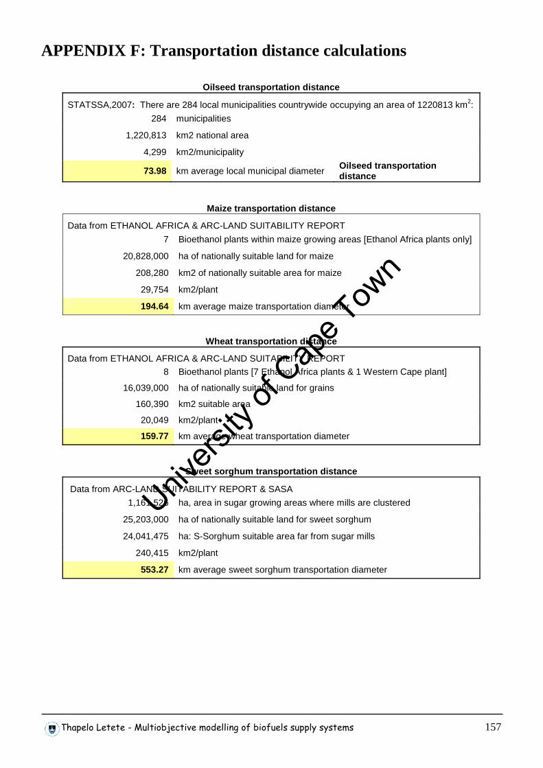
Thapelo Letete - Multiobjective modelling of biofuels supply systems 157
APPENDIX F: Transportation distance calculations
Oilseed transportation distance
STATSSA,2007: There are 284 local municipalities countrywide occupying an area of 1220813 km2:
284 municipalities
1,220,813 km2 national area
4,299 km2/municipality
73.98 km average local municipal diameter Oilseed transportation distance
Maize transportation distance
Data from ETHANOL AFRICA & ARC-LAND SUITABILITY REPORT
7 Bioethanol plants within maize growing areas [Ethanol Africa plants only]
20,828,000 ha of nationally suitable land for maize
208,280 km2 of nationally suitable area for maize
29,754 km2/plant
194.64 km average maize transportation diameter
Wheat transportation distance
Data from ETHANOL AFRICA & ARC-LAND SUITABILITY REPORT
8 Bioethanol plants [7 Ethanol Africa plants & 1 Western Cape plant]
16,039,000 ha of nationally suitable land for grains
160,390 km2 suitable area
20,049 km2/plant
159.77 km average wheat transportation diameter
Sweet sorghum transportation distance
Data from ARC-LAND SUITABILITY REPORT & SASA
1,161,526 ha, area in sugar growing areas where mills are clustered
25,203,000 ha of nationally suitable land for sweet sorghum
24,041,475 ha: S-Sorghum suitable area far from sugar mills
240,415 km2/plant
553.27 km average sweet sorghum transportation diameter
Univers
ity of
Cap
e Tow
n
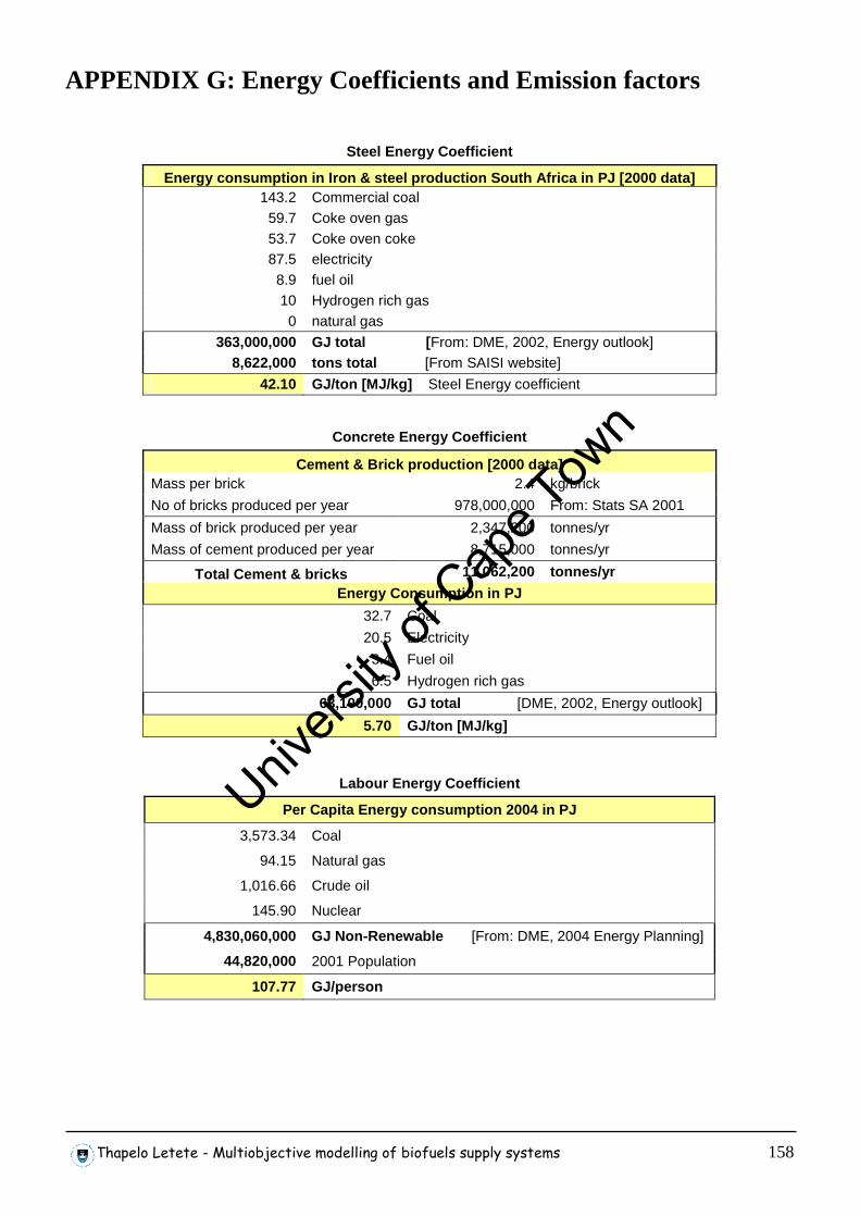
Thapelo Letete - Multiobjective modelling of biofuels supply systems 158
APPENDIX G: Energy Coefficients and Emission factors
Steel Energy Coefficient
Energy consumption in Iron & steel production South Africa in PJ [2000 data] 143.2 Commercial coal
59.7 Coke oven gas 53.7 Coke oven coke 87.5 electricity 8.9 fuel oil 10 Hydrogen rich gas 0 natural gas
363,000,000 GJ total [ From: DME, 2002, Energy outlook] 8,622,000 tons total [From SAISI website]
42.10 GJ/ton [MJ/kg] Steel Energy coefficient
Concrete Energy Coefficient
Cement & Brick production [2000 data] Mass per brick 2.4 kg/brick
No of bricks produced per year 978,000,000 From: Stats SA 2001
Mass of brick produced per year 2,347,200 tonnes/yr
Mass of cement produced per year 8,715,000 tonnes/yr
Total Cement & bricks 11,062,200 tonnes/yr
Energy Consumption in PJ
32.7 Coal
20.5 Electricity
3.4 Fuel oil
6.5 Hydrogen rich gas
63,100,000 GJ total [DME, 2002, Energy outlook]
5.70 GJ/ton [MJ/kg]
Labour Energy Coefficient
Per Capita Energy consumption 2004 in PJ
3,573.34 Coal
94.15 Natural gas
1,016.66 Crude oil
145.90 Nuclear
4,830,060,000 GJ Non-Renewable [From: DME, 2004 Energy Planning]
44,820,000 2001 Population
107.77 GJ/person
Univers
ity of
Cap
e Tow
n
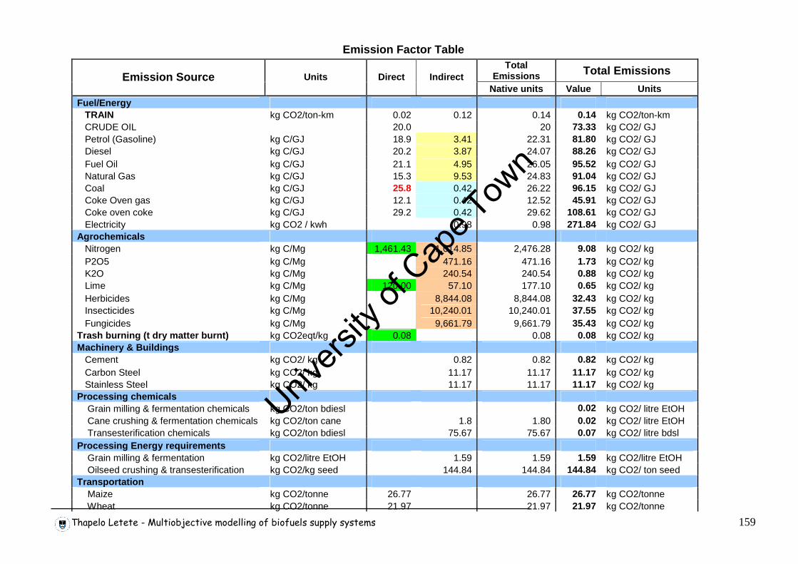
Thapelo Letete - Multiobjective modelling of biofuels supply systems 159
Emission Factor Table Total
Emissions Total Emissions Emission Source Units Direct Indirect Native units Value Units
Fuel/Energy TRAIN kg CO2/ton-km 0.02 0.12 0.14 0.14 kg CO2/ton-km CRUDE OIL 20.0 20 73.33 kg CO2/ GJ Petrol (Gasoline) kg C/GJ 18.9 3.41 22.31 81.80 kg CO2/ GJ Diesel kg C/GJ 20.2 3.87 24.07 88.26 kg CO2/ GJ Fuel Oil kg C/GJ 21.1 4.95 26.05 95.52 kg CO2/ GJ Natural Gas kg C/GJ 15.3 9.53 24.83 91.04 kg CO2/ GJ Coal kg C/GJ 25.8 0.42 26.22 96.15 kg CO2/ GJ Coke Oven gas kg C/GJ 12.1 0.42 12.52 45.91 kg CO2/ GJ Coke oven coke kg C/GJ 29.2 0.42 29.62 108.61 kg CO2/ GJ Electricity kg CO2 / kwh 0.98 0.98 271.84 kg CO2/ GJ Agrochemicals Nitrogen kg C/Mg 1,461.43 1,014.85 2,476.28 9.08 kg CO2/ kg P2O5 kg C/Mg 471.16 471.16 1.73 kg CO2/ kg K2O kg C/Mg 240.54 240.54 0.88 kg CO2/ kg Lime kg C/Mg 120.00 57.10 177.10 0.65 kg CO2/ kg Herbicides kg C/Mg 8,844.08 8,844.08 32.43 kg CO2/ kg Insecticides kg C/Mg 10,240.01 10,240.01 37.55 kg CO2/ kg Fungicides kg C/Mg 9,661.79 9,661.79 35.43 kg CO2/ kg Trash burning (t dry matter burnt) kg CO2eqt/kg 0.08 0.08 0.08 kg CO2/ kg Machinery & Buildings Cement kg CO2/ kg 0.82 0.82 0.82 kg CO2/ kg Carbon Steel kg CO2/ kg 11.17 11.17 11.17 kg CO2/ kg Stainless Steel kg CO2/ kg 11.17 11.17 11.17 kg CO2/ kg Processing chemicals Grain milling & fermentation chemicals kg CO2/ton bdiesl 0.02 kg CO2/ litre EtOH Cane crushing & fermentation chemicals kg CO2/ton cane 1.8 1.80 0.02 kg CO2/ litre EtOH Transesterification chemicals kg CO2/ton bdiesl 75.67 75.67 0.07 kg CO2/ litre bdsl Processing Energy requirements Grain milling & fermentation kg CO2/litre EtOH 1.59 1.59 1.59 kg CO2/litre EtOH Oilseed crushing & transesterification kg CO2/kg seed 144.84 144.84 144.84 kg CO2/ ton seed Transportation Maize kg CO2/tonne 26.77 26.77 26.77 kg CO2/tonne Wheat kg CO2/tonne 21.97 21.97 21.97 kg CO2/tonne
Univers
ity of
Cap
e Tow
n
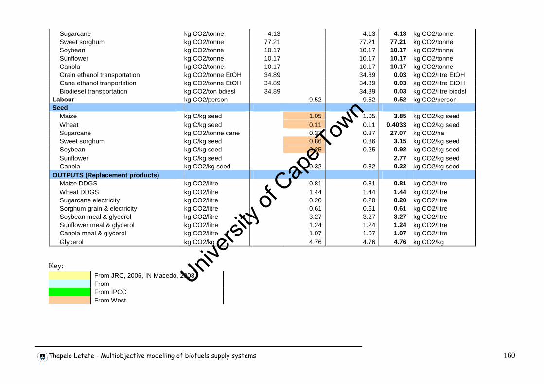
Thapelo Letete - Multiobjective modelling of biofuels supply systems 160
Sugarcane kg CO2/tonne 4.13 4.13 4.13 kg CO2/tonne Sweet sorghum kg CO2/tonne 77.21 77.21 77.21 kg CO2/tonne Soybean kg CO2/tonne 10.17 10.17 10.17 kg CO2/tonne Sunflower kg CO2/tonne 10.17 10.17 10.17 kg CO2/tonne Canola kg CO2/tonne 10.17 10.17 10.17 kg CO2/tonne Grain ethanol transportation kg CO2/tonne EtOH 34.89 34.89 0.03 kg CO2/litre EtOH Cane ethanol tranportation kg CO2/tonne EtOH 34.89 34.89 0.03 kg CO2/litre EtOH Biodiesel transportation kg CO2/ton bdiesl 34.89 34.89 0.03 kg CO2/litre biodsl Labour kg CO2/person 9.52 9.52 9.52 kg CO2/person Seed Maize kg C/kg seed 1.05 1.05 3.85 kg CO2/kg seed Wheat kg C/kg seed 0.11 0.11 0.4033 kg CO2/kg seed Sugarcane kg CO2/tonne cane 0.37 0.37 27.07 kg CO2/ha Sweet sorghum kg C/kg seed 0.86 0.86 3.15 kg CO2/kg seed Soybean kg C/kg seed 0.25 0.25 0.92 kg CO2/kg seed Sunflower kg C/kg seed 2.77 kg CO2/kg seed Canola kg CO2/kg seed 0.32 0.32 0.32 kg CO2/kg seed OUTPUTS (Replacement products) Maize DDGS kg CO2/litre 0.81 0.81 0.81 kg CO2/litre Wheat DDGS kg CO2/litre 1.44 1.44 1.44 kg CO2/litre Sugarcane electricity kg CO2/litre 0.20 0.20 0.20 kg CO2/litre Sorghum grain & electricity kg CO2/litre 0.61 0.61 0.61 kg CO2/litre Soybean meal & glycerol kg CO2/litre 3.27 3.27 3.27 kg CO2/litre Sunflower meal & glycerol kg CO2/litre 1.24 1.24 1.24 kg CO2/litre Canola meal & glycerol kg CO2/litre 1.07 1.07 1.07 kg CO2/litre Glycerol kg CO2/kg 4.76 4.76 4.76 kg CO2/kg
Key:
From JRC, 2006, IN Macedo, 2008 From From IPCC From West
Univers
ity of
Cap
e Tow
n
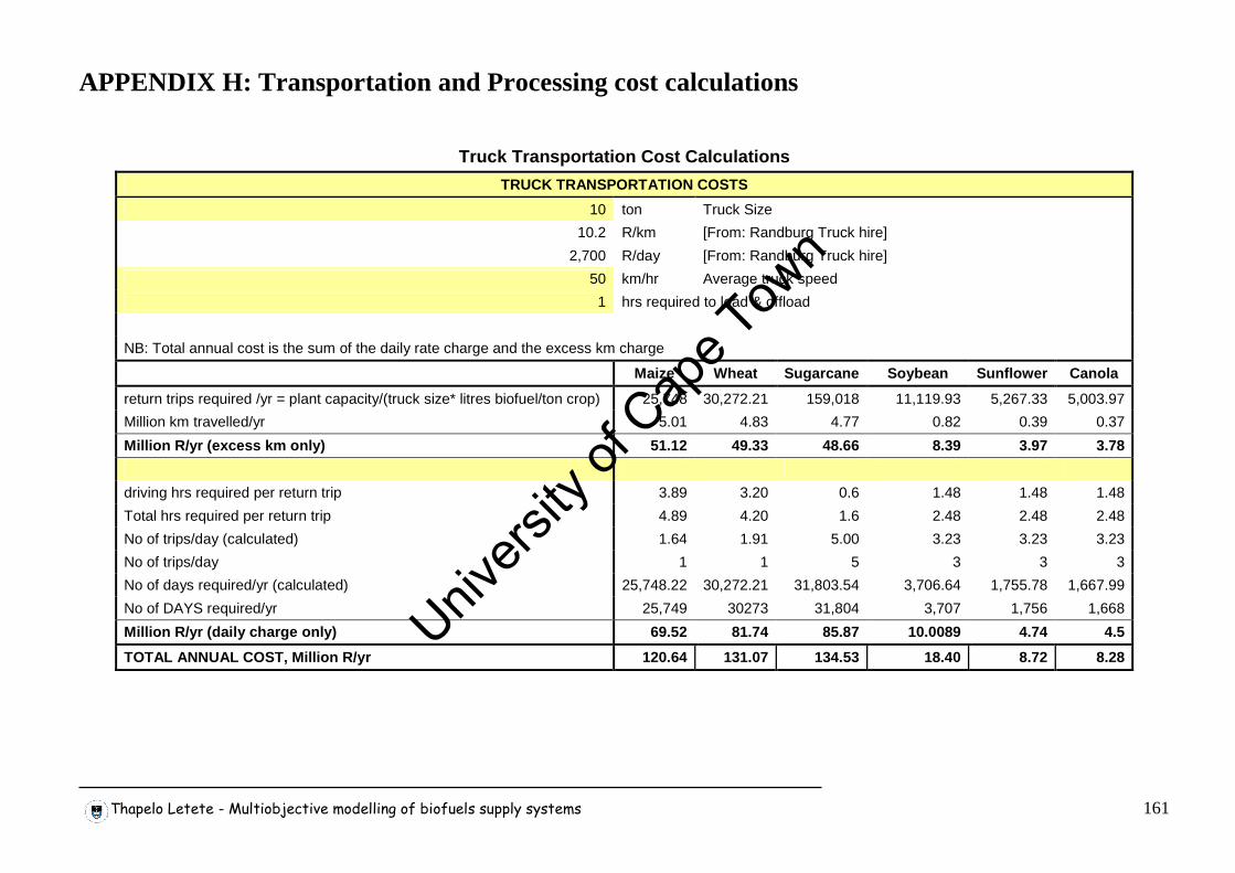
Thapelo Letete - Multiobjective modelling of biofuels supply systems 161
APPENDIX H: Transportation and Processing cost calculations
Truck Transportation Cost Calculations
TRUCK TRANSPORTATION COSTS
10 ton Truck Size
10.2 R/km [From: Randburg Truck hire]
2,700 R/day [From: Randburg Truck hire]
50 km/hr Average truck speed
1 hrs required to load & offload
NB: Total annual cost is the sum of the daily rate charge and the excess km charge
Maize Wheat Sugarcane Soybean Sunflower Canola
return trips required /yr = plant capacity/(truck size* litres biofuel/ton crop) 25,748 30,272.21 159,018 11,119.93 5,267.33 5,003.97
Million km travelled/yr 5.01 4.83 4.77 0.82 0.39 0.37
Million R/yr (excess km only) 51.12 49.33 48.66 8.39 3.97 3.78
driving hrs required per return trip 3.89 3.20 0.6 1.48 1.48 1.48
Total hrs required per return trip 4.89 4.20 1.6 2.48 2.48 2.48
No of trips/day (calculated) 1.64 1.91 5.00 3.23 3.23 3.23
No of trips/day 1 1 5 3 3 3
No of days required/yr (calculated) 25,748.22 30,272.21 31,803.54 3,706.64 1,755.78 1,667.99
No of DAYS required/yr 25,749 30273 31,804 3,707 1,756 1,668
Million R/yr (daily charge only) 69.52 81.74 85.87 10.0089 4.74 4.5
TOTAL ANNUAL COST, Million R/yr 120.64 131.07 134.53 18.40 8.72 8.28
Univ
ersity
of C
ape T
own
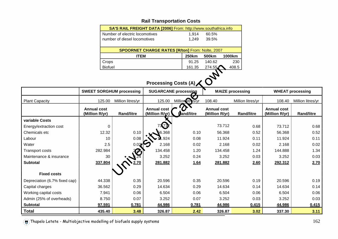
Thapelo Letete - Multiobjective modelling of biofuels supply systems 162
Rail Transportation Costs
SA'S RAIL FREIGHT DATA [2006] From: http://www.southafrica.info Number of electric locomotives 1,914 60.5% number of diesel locomotives 1,249 39.5%
SPOORNET CHARGE RATES [R/ton] From: Nolte, 2007 ITEM 250km 500km 1000km
Crops 91.25 140.62 230 Biofuel 161.35 274.55 408.5
Processing Costs (A)
SWEET SORGHUM processing SUGARCANE processing MAIZE processing WHEAT processing
Plant Capacity 125.00 Million litres/yr 125.00 Million litres/yr 108.40 Million litres/yr 108.40 Million litres/yr
Annual cost (Million R/yr) Rand/litre
Annual cost (Million R/yr) Rand/litre
Annual cost (Million R/yr) Rand/litre
Annual cost (Million R/yr) Rand/litre
variable Costs
Energy/extraction cost 0 73.712 73.712 0.68 73.712 0.68
Chemicals etc 12.32 0.10 56.368 0.10 56.368 0.52 56.368 0.52
Labour 10 0.08 11.924 0.08 11.924 0.11 11.924 0.11
Water 2.5 0.02 2.168 0.02 2.168 0.02 2.168 0.02
Transport costs 282.984 2.26 134.458 1.20 134.458 1.24 144.888 1.34
Maintenance & insurance 30 0.24 3.252 0.24 3.252 0.03 3.252 0.03
Subtotal 337.804 2.70 281.882 1.64 281.882 2.60 292.312 2.70
Fixed costs
Depreciation (6.7% fixed cap) 44.338 0.35 20.596 0.35 20.596 0.19 20.596 0.19
Capital charges 36.562 0.29 14.634 0.29 14.634 0.14 14.634 0.14
Working capital costs 7.941 0.06 6.504 0.06 6.504 0.06 6.504 0.06
Admin (25% of overheads) 8.750 0.07 3.252 0.07 3.252 0.03 3.252 0.03
Subtotal 97.591 0.781 44.986 0.781 44.986 0.415 44.986 0.415
Total 435.40 3.48 326.87 2.42 326.87 3.02 337.30 3.11
Univers
ity of
Cap
e Tow
n
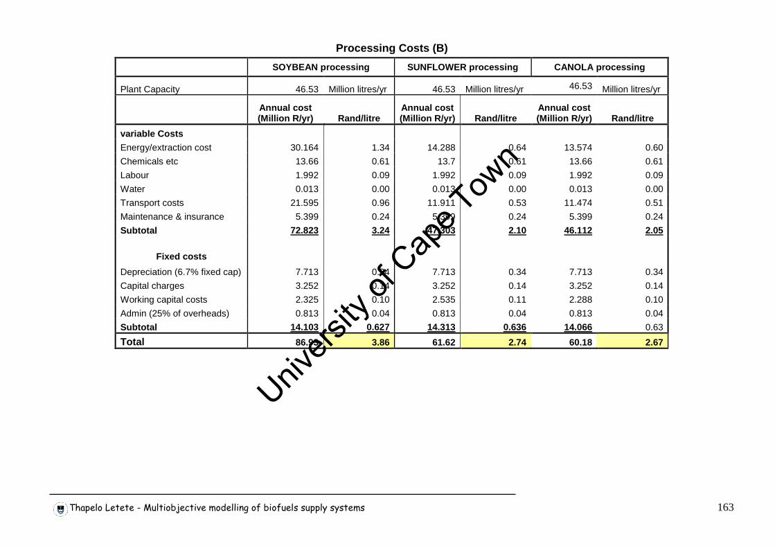
Thapelo Letete - Multiobjective modelling of biofuels supply systems 163
Processing Costs (B)
SOYBEAN processing SUNFLOWER processing CANOLA processing
Plant Capacity 46.53 Million litres/yr 46.53 Million litres/yr 46.53 Million litres/yr
Annual cost (Million R/yr) Rand/litre
Annual cost (Million R/yr) Rand/litre
Annual cost (Million R/yr) Rand/litre
variable Costs
Energy/extraction cost 30.164 1.34 14.288 0.64 13.574 0.60
Chemicals etc 13.66 0.61 13.7 0.61 13.66 0.61
Labour 1.992 0.09 1.992 0.09 1.992 0.09
Water 0.013 0.00 0.013 0.00 0.013 0.00
Transport costs 21.595 0.96 11.911 0.53 11.474 0.51
Maintenance & insurance 5.399 0.24 5.399 0.24 5.399 0.24
Subtotal 72.823 3.24 47.303 2.10 46.112 2.05
Fixed costs
Depreciation (6.7% fixed cap) 7.713 0.34 7.713 0.34 7.713 0.34
Capital charges 3.252 0.14 3.252 0.14 3.252 0.14
Working capital costs 2.325 0.10 2.535 0.11 2.288 0.10
Admin (25% of overheads) 0.813 0.04 0.813 0.04 0.813 0.04
Subtotal 14.103 0.627 14.313 0.636 14.066 0.63
Total 86.93 3.86 61.62 2.74 60.18 2.67
Univers
ity of
Cap
e Tow
n
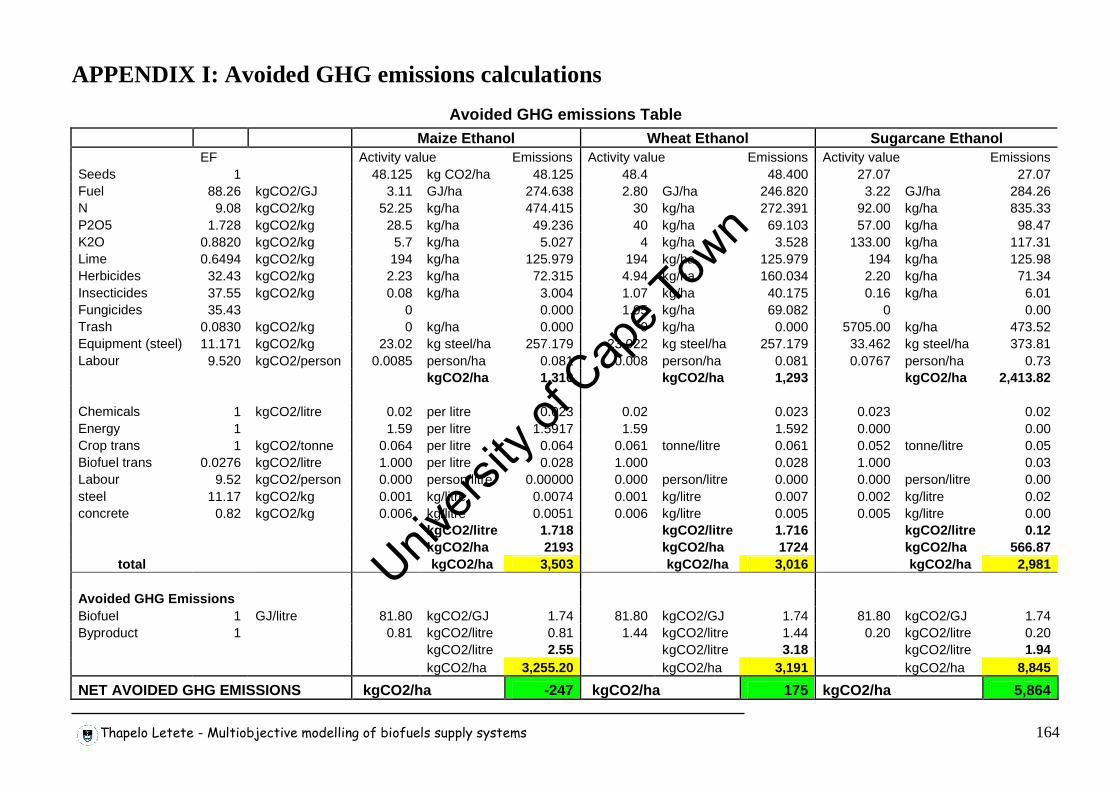
Thapelo Letete - Multiobjective modelling of biofuels supply systems 164
APPENDIX I: Avoided GHG emissions calculations
Avoided GHG emissions Table
Maize Ethanol Wheat Ethanol Sugarcane Ethanol EF Activity value Emissions Activity value Emissions Activity value Emissions Seeds 1 48.125 kg CO2/ha 48.125 48.4 48.400 27.07 27.07 Fuel 88.26 kgCO2/GJ 3.11 GJ/ha 274.638 2.80 GJ/ha 246.820 3.22 GJ/ha 284.26 N 9.08 kgCO2/kg 52.25 kg/ha 474.415 30 kg/ha 272.391 92.00 kg/ha 835.33 P2O5 1.728 kgCO2/kg 28.5 kg/ha 49.236 40 kg/ha 69.103 57.00 kg/ha 98.47 K2O 0.8820 kgCO2/kg 5.7 kg/ha 5.027 4 kg/ha 3.528 133.00 kg/ha 117.31 Lime 0.6494 kgCO2/kg 194 kg/ha 125.979 194 kg/ha 125.979 194 kg/ha 125.98 Herbicides 32.43 kgCO2/kg 2.23 kg/ha 72.315 4.94 kg/ha 160.034 2.20 kg/ha 71.34 Insecticides 37.55 kgCO2/kg 0.08 kg/ha 3.004 1.07 kg/ha 40.175 0.16 kg/ha 6.01 Fungicides 35.43 0 0.000 1.95 kg/ha 69.082 0 0.00 Trash 0.0830 kgCO2/kg 0 kg/ha 0.000 0 kg/ha 0.000 5705.00 kg/ha 473.52 Equipment (steel) 11.171 kgCO2/kg 23.02 kg steel/ha 257.179 23.022 kg steel/ha 257.179 33.462 kg steel/ha 373.81 Labour 9.520 kgCO2/person 0.0085 person/ha 0.081 0.008 person/ha 0.081 0.0767 person/ha 0.73 kgCO2/ha 1,310 kgCO2/ha 1,293 kgCO2/ha 2,413.82 Chemicals 1 kgCO2/litre 0.02 per litre 0.023 0.02 0.023 0.023 0.02 Energy 1 1.59 per litre 1.5917 1.59 1.592 0.000 0.00 Crop trans 1 kgCO2/tonne 0.064 per litre 0.064 0.061 tonne/litre 0.061 0.052 tonne/litre 0.05 Biofuel trans 0.0276 kgCO2/litre 1.000 per litre 0.028 1.000 0.028 1.000 0.03 Labour 9.52 kgCO2/person 0.000 person/litre 0.00000 0.000 person/litre 0.000 0.000 person/litre 0.00 steel 11.17 kgCO2/kg 0.001 kg/litre 0.0074 0.001 kg/litre 0.007 0.002 kg/litre 0.02 concrete 0.82 kgCO2/kg 0.006 kg/litre 0.0051 0.006 kg/litre 0.005 0.005 kg/litre 0.00 kgCO2/litre 1.718 kgCO2/litre 1.716 kgCO2/litre 0.12 kgCO2/ha 2193 kgCO2/ha 1724 kgCO2/ha 566.87
total kgCO2/ha 3,503 kgCO2/ha 3,016 kgCO2/ha 2,981 Avoided GHG Emissions Biofuel 1 GJ/litre 81.80 kgCO2/GJ 1.74 81.80 kgCO2/GJ 1.74 81.80 kgCO2/GJ 1.74 Byproduct 1 0.81 kgCO2/litre 0.81 1.44 kgCO2/litre 1.44 0.20 kgCO2/litre 0.20 kgCO2/litre 2.55 kgCO2/litre 3.18 kgCO2/litre 1.94 kgCO2/ha 3,255.20 kgCO2/ha 3,191 kgCO2/ha 8,845
NET AVOIDED GHG EMISSIONS kgCO2/ha -247 kgCO2/ha 175 kgCO2/ha 5,864 Univ
ersity
of C
ape T
own
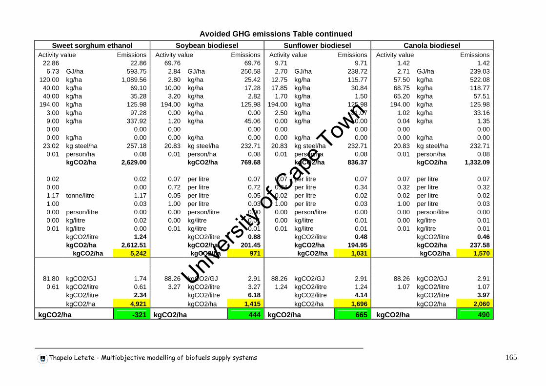
Thapelo Letete - Multiobjective modelling of biofuels supply systems 165
Avoided GHG emissions Table continued
Sweet sorghum ethanol Soybean biodiesel Sunflower bi odiesel Canola biodiesel Activity value Emissions Activity value Emissions Activity value Emissions Activity value Emissions
22.86 22.86 69.76 69.76 9.71 9.71 1.42 1.42 6.73 GJ/ha 593.75 2.84 GJ/ha 250.58 2.70 GJ/ha 238.72 2.71 GJ/ha 239.03
120.00 kg/ha 1,089.56 2.80 kg/ha 25.42 12.75 kg/ha 115.77 57.50 kg/ha 522.08 40.00 kg/ha 69.10 10.00 kg/ha 17.28 17.85 kg/ha 30.84 68.75 kg/ha 118.77 40.00 kg/ha 35.28 3.20 kg/ha 2.82 1.70 kg/ha 1.50 65.20 kg/ha 57.51
194.00 kg/ha 125.98 194.00 kg/ha 125.98 194.00 kg/ha 125.98 194.00 kg/ha 125.98 3.00 kg/ha 97.28 0.00 kg/ha 0.00 2.50 kg/ha 81.07 1.02 kg/ha 33.16 9.00 kg/ha 337.92 1.20 kg/ha 45.06 0.00 kg/ha 0.00 0.04 kg/ha 1.35 0.00 0.00 0.00 0.00 0.00 0.00 0.00 0.00 0.00 kg/ha 0.00 0.00 kg/ha 0.00 0.00 kg/ha 0.00 0.00 kg/ha 0.00
23.02 kg steel/ha 257.18 20.83 kg steel/ha 232.71 20.83 kg steel/ha 232.71 20.83 kg steel/ha 232.71 0.01 person/ha 0.08 0.01 person/ha 0.08 0.01 person/ha 0.08 0.01 person/ha 0.08
kgCO2/ha 2,629.00 kgCO2/ha 769.68 kgCO2/ha 836.37 kgCO2/ha 1,332.09
0.02 0.02 0.07 per litre 0.07 0.07 per litre 0.07 0.07 per litre 0.07 0.00 0.00 0.72 per litre 0.72 0.34 per litre 0.34 0.32 per litre 0.32 1.17 tonne/litre 1.17 0.05 per litre 0.05 0.02 per litre 0.02 0.02 per litre 0.02 1.00 0.03 1.00 per litre 0.03 1.00 per litre 0.03 1.00 per litre 0.03 0.00 person/litre 0.00 0.00 person/litre 0.00 0.00 person/litre 0.00 0.00 person/litre 0.00 0.00 kg/litre 0.02 0.00 kg/litre 0.01 0.00 kg/litre 0.01 0.00 kg/litre 0.01 0.01 kg/litre 0.00 0.01 kg/litre 0.01 0.01 kg/litre 0.01 0.01 kg/litre 0.01
kgCO2/litre 1.24 kgCO2/litre 0.88 kgCO2/litre 0.48 kgCO2/litre 0.46 kgCO2/ha 2,612.51 kgCO2/ha 201.45 kgCO2/ha 194.95 kgCO2/ha 237.58
kgCO2/ha 5,242 kgCO2/ha 971 kgCO2/ha 1,031 kgCO2/ha 1,570
81.80 kgCO2/GJ 1.74 88.26 kgCO2/GJ 2.91 88.26 kgCO2/GJ 2.91 88.26 kgCO2/GJ 2.91 0.61 kgCO2/litre 0.61 3.27 kgCO2/litre 3.27 1.24 kgCO2/litre 1.24 1.07 kgCO2/litre 1.07
kgCO2/litre 2.34 kgCO2/litre 6.18 kgCO2/litre 4.14 kgCO2/litre 3.97 kgCO2/ha 4,921 kgCO2/ha 1,415 kgCO2/ha 1,696 kgCO2/ha 2,060
kgCO2/ha -321 kgCO2/ha 444 kgCO2/ha 665 kgCO2/ha 490
Univers
ity of
Cap
e Tow
n
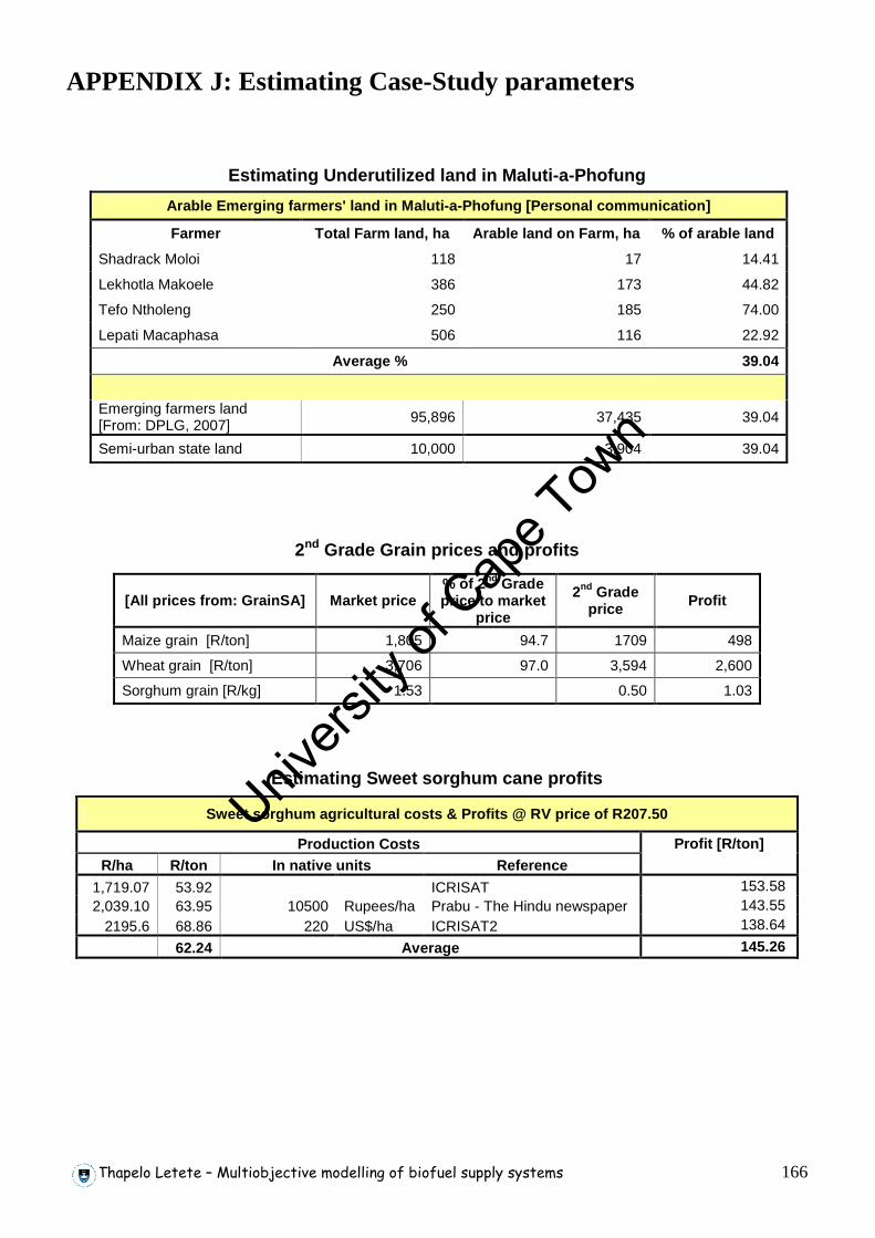
Thapelo Letete – Multiobjective modelling of biofuel supply systems 166
APPENDIX J: Estimating Case-Study parameters
Estimating Underutilized land in Maluti-a-Phofung
2nd Grade Grain prices and profits
Estimating Sweet sorghum cane profits
Sweet sorghum agricultural costs & Profits @ RV price of R207.50
Production Costs R/ha R/ton In native units Reference
Profit [R/ton]
1,719.07 53.92 ICRISAT 153.58 2,039.10 63.95 10500 Rupees/ha Prabu - The Hindu newspaper 143.55
2195.6 68.86 220 US$/ha ICRISAT2 138.64
62.24 Average 145.26
Arable Emerging farmers' land in Maluti-a-Phofung [Personal communication]
Farmer Total Farm land, ha Arable land on Farm, ha % of arable land
Shadrack Moloi 118 17 14.41
Lekhotla Makoele 386 173 44.82
Tefo Ntholeng 250 185 74.00
Lepati Macaphasa 506 116 22.92
Average % 39.04
Emerging farmers land [From: DPLG, 2007] 95,896 37,435 39.04
Semi-urban state land 10,000 3,904 39.04
[All prices from: GrainSA] Market price % of 2 nd Grade price to market
price
2nd Grade price Profit
Maize grain [R/ton] 1,805 94.7 1709 498
Wheat grain [R/ton] 3,706 97.0 3,594 2,600
Sorghum grain [R/kg] 1.53 0.50 1.03
Univers
ity of
Cap
e Tow
n
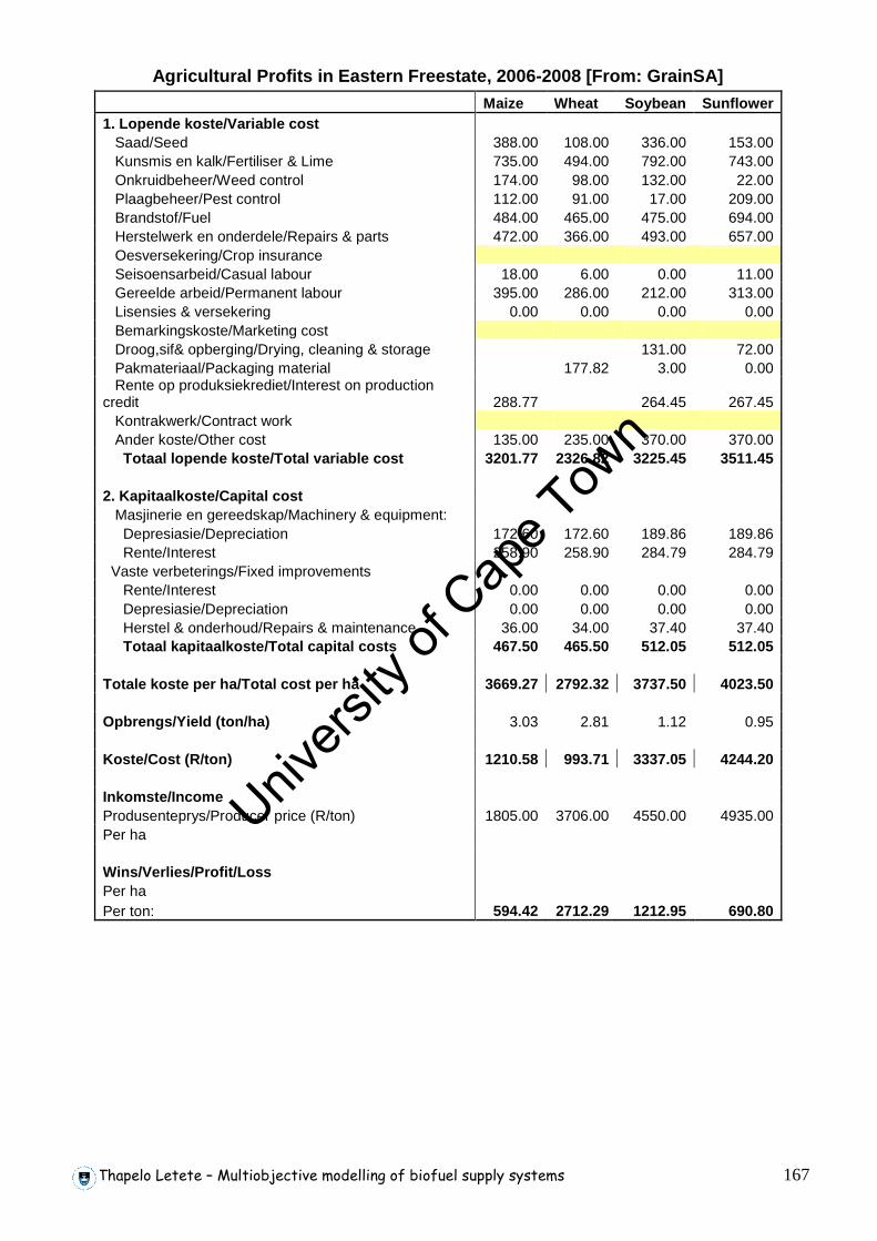
Thapelo Letete – Multiobjective modelling of biofuel supply systems 167
Agricultural Profits in Eastern Freestate, 2006-2008 [From: GrainSA]
Maize Wheat Soybean Sunflower 1. Lopende koste/Variable cost Saad/Seed 388.00 108.00 336.00 153.00 Kunsmis en kalk/Fertiliser & Lime 735.00 494.00 792.00 743.00 Onkruidbeheer/Weed control 174.00 98.00 132.00 22.00 Plaagbeheer/Pest control 112.00 91.00 17.00 209.00 Brandstof/Fuel 484.00 465.00 475.00 694.00 Herstelwerk en onderdele/Repairs & parts 472.00 366.00 493.00 657.00 Oesversekering/Crop insurance Seisoensarbeid/Casual labour 18.00 6.00 0.00 11.00 Gereelde arbeid/Permanent labour 395.00 286.00 212.00 313.00 Lisensies & versekering 0.00 0.00 0.00 0.00 Bemarkingskoste/Marketing cost Droog,sif& opberging/Drying, cleaning & storage 131.00 72.00 Pakmateriaal/Packaging material 177.82 3.00 0.00 Rente op produksiekrediet/Interest on production credit 288.77 264.45 267.45 Kontrakwerk/Contract work Ander koste/Other cost 135.00 235.00 370.00 370.00 Totaal lopende koste/Total variable cost 3201.77 2326.82 3225.45 3511.45 2. Kapitaalkoste/Capital cost Masjinerie en gereedskap/Machinery & equipment: Depresiasie/Depreciation 172.60 172.60 189.86 189.86 Rente/Interest 258.90 258.90 284.79 284.79 Vaste verbeterings/Fixed improvements Rente/Interest 0.00 0.00 0.00 0.00 Depresiasie/Depreciation 0.00 0.00 0.00 0.00 Herstel & onderhoud/Repairs & maintenance 36.00 34.00 37.40 37.40 Totaal kapitaalkoste/Total capital costs 467.50 465.50 512.05 512.05 Totale koste per ha/Total cost per ha 3669.27 2792.32 3737.50 4023.50 Opbrengs/Yield (ton/ha) 3.03 2.81 1.12 0.95 Koste/Cost (R/ton) 1210.58 993.71 3337.05 4244.20 Inkomste/Income Produsenteprys/Producer price (R/ton) 1805.00 3706.00 4550.00 4935.00 Per ha Wins/Verlies/Profit/Loss Per ha Per ton: 594.42 2712.29 1212.95 690.80
Univers
ity of
Cap
e Tow
n
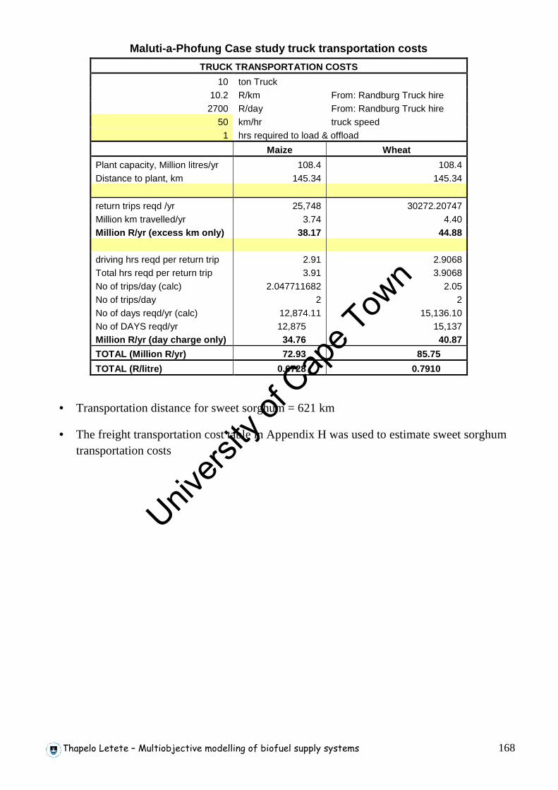
Thapelo Letete – Multiobjective modelling of biofuel supply systems 168
Maluti-a-Phofung Case study truck transportation costs
TRUCK TRANSPORTATION COSTS
10 ton Truck 10.2 R/km From: Randburg Truck hire 2700 R/day From: Randburg Truck hire
50 km/hr truck speed 1 hrs required to load & offload
Maize Wheat
Plant capacity, Million litres/yr 108.4 108.4 Distance to plant, km 145.34 145.34
return trips reqd /yr 25,748 30272.20747 Million km travelled/yr 3.74 4.40 Million R/yr (excess km only) 38.17 44.88 driving hrs reqd per return trip 2.91 2.9068 Total hrs reqd per return trip 3.91 3.9068 No of trips/day (calc) 2.047711682 2.05 No of trips/day 2 2 No of days reqd/yr (calc) 12,874.11 15,136.10 No of DAYS reqd/yr 12,875 15,137 Million R/yr (day charge only) 34.76 40.87
TOTAL (Million R/yr) 72.93 85.75
TOTAL (R/litre) 0.6728 0.7910
• Transportation distance for sweet sorghum = 621 km
• The freight transportation cost table in Appendix H was used to estimate sweet sorghum transportation costs
Univers
ity of
Cap
e Tow
n