multiobjective learner performance-based behavior ... - arxiv
TRANSCRIPT
Cite as: Rahman, C.M., Rashid, T.A., Ahmed, A.M., Seyedali Mirjalili (2022) Multi-objective learner performance-based behavior algorithm with five multi-objective real-world engineering problems. Neural Comput & Applic . https://doi.org/10.1007/s00521-021-06811-z
1
Multiobjective Learner Performance-based Behavior Algorithm with Five Multiobjective Real-world Engineering Problems
Chnoor M. Rahman1, Tarik A. Rashid2, Aram Mahmood Ahmed3, 4 , Seyedali Mirjalili5,6
1 Applied Computer Department, College of Medicals and Applied Sciences, Charmo University, Sulaimany, Iraq. 2 Computer Science and Engineering Department, University of Kurdistan Hewler, Erbil, Iraq. 3 Department of Information Technology, Technical College of Informatics, Sulaimani Polytechnic University, Sulaimany, Iraq. 4 Department of Information Technology, College of Science and Technology, University of Human Development. Sulaimany,
Iraq. 5Centre for Artificial Intelligence Research and Optimization, Torrens University, Australia. 6Yonsei Frontier Lab, Yonsei University, Seoul, Korea.
Abstract In this work, a new multiobjective optimization algorithm called multiobjective learner performance-based behavior
algorithm is proposed. The proposed algorithm is based on the process of transferring students from high school to
college. The proposed technique produces a set of non-dominated solutions. To judge the ability and efficacy of the
proposed multiobjective algorithm, it is evaluated against a group of benchmarks and five real-world engineering
optimization problems. Additionally, to evaluate the proposed technique quantitatively, several most widely used
metrics are applied. Moreover, the results are confirmed statistically. The proposed work is then compared with
three multiobjective algorithms, which are MOWCA, NSGA-II, and MODA. Similar to the proposed technique, the
other algorithms in the literature were run against the benchmarks, and the real-world engineering problems utilized
in the paper. The algorithms are compared with each other employing descriptive, tabular, and graphical
demonstrations. The results proved the ability of the proposed work in providing a set of non-dominated solutions,
and that the algorithm outperformed the other participated algorithms in most of the cases.
Keywords Multiobjective Algorithms, Multiobjective Evolutionary Algorithms, MOLPB, LPB, Learner Performance-Based
Behavior Algorithm, Optimization, Metaheuristic Optimization Algorithm
1. Introduction During the last few decades, some techniques have been proposed to solve engineering optimization problems. The
majority of the techniques were based on nonlinear and linear programming methods. They can find the global
optimum for simple to medium problems. An immense number of real-world optimization problems have more than
one objective function to maximize and/or minimize. These objectives are often conflicting. Biological disciplines,
economic, engineering, and automotive problems are examples of such real-world problems. Thus, since the 1970s,
researchers have been interested in examining multiobjective optimization algorithms (MOAs); see [1-6]. However,
until preparing this paper, no single approach exists to tackle all the various problems with a huge number of
conflicting objectives. While we use the MOAs it is difficult to find one utopian solution which satisfies all the
conflicting objectives. This is because that utopian solution may satisfy one objective, or a subset of the objectives
whilst provides poor regarding another objective, or a subset of objectives. Hence, the MOAs provides a set of
tradeoff solutions instead of one utopian solution. The produced set is known as the non-dominated solution set or
Pareto optimal solution set. The non-dominated solution set provides solutions with a tradeoff that satisfy all the
conflicting objectives without violating any of the existing constraints. The individual solutions in the non-
dominated set are called Pareto optimum. All the Pareto optimum solutions are optimal, and compared to the
optimum solutions no better solutions exist in the search space when considering all the objectives. None of the
Pareto optimum solutions is better than another Pareto optimum solution. However, based on some other
information, which is related to the demands of the problem owner, the problem owner can decide which of the
Cite as: Rahman, C.M., Rashid, T.A., Ahmed, A.M., Seyedali Mirjalili (2022) Multi-objective learner performance-based behavior algorithm with five multi-objective real-world engineering problems. Neural Comput & Applic . https://doi.org/10.1007/s00521-021-06811-z
2
Pareto optimum solutions is better. Hence, finding as many Pareto optimum solutions as possible is necessary. Thus,
MOAs may produce an infinite number of optimal solutions. Plotting the Pareto optimum solutions produce a Pareto
front. The foremost goal of MOAs is to produce a Pareto front for the provided multiobjective optimization problem
(MOP) [7, 8].
Optimization algorithms, in general, are utilized to optimize various problems in various fields. For example, in [9],
a genetic algorithm (GA) was combined with interior point techniques (IPTs) to optimize a new approach that solves
the initial value of the equation of a Painlev´e II, and its variants, utilizing the feed-forward artificial network. The
GA was utilized as a global search technique to optimize the weights of the artificial neural network, and the IPTs
were utilized as a local search technique. The proposed model was validated using relative investigation with plain
Range-Kutta numerical process on nonlinear Painlev´e II through utilizing various magnitudes of forcing factors.
The reason for proposing the technique (GA-IPT) was that with enlarging the iterations, the GA’s ability to optimize
the solutions was reduced, and the improvements in the solutions for a big number of iterations were not reasonable.
Hence, the researchers utilized an effective local search technique to reduce the drawbacks of the global search
technique for the proposed work. The hybrid method utilized in the work was efficient; however, it was more prone
to different runs. Similarly, the study [10] designed a neuro-heuristic schema for the non-linear second order
Thomas-Fermi system. To optimize the schema, the GA and sequential quadratic programming were utilized, and it
was discovered that the examined schema was feasible, precise, and effective. In [11], a salp swarm algorithm (SSA)
with Jaya optimizer was used to optimize the parameters of temperature effect in dam health monitoring utilizing
support vector machines. Jaya and SSA were utilized as search engines to select the parameters of least square
support vector machines (LSSVM) and support vector machines (SVM). In the proposed work, a hybrid technique
was examined to predict the behaviors of concrete dams. The work discussed the influence of incorporating
measured temperatures into the model rather than utilizing a model with indirect temperature. The results proved
that the proposed model has a small value of prediction errors and residuals.
Evolutionary algorithms (EAs) are excellent examples of optimization algorithms. EAs are stochastic and global
search methods. They symbolize the concept of natural selection and the endurance of the fittest. It has been proven
that EAs are powerful and robust search techniques [12, 13]. They excel at finding many tradeoff solutions in the
sole run. Additionally, due to their ability to explore the large promising region and solve problems with many
conflicting objectives, the EAs are well suited to solve MOPs. Hence, one of the effective approaches to solve
MOPs is evolutionary multiobjective optimization algorithms (EMOAs). However, EMOAs usually need a large
number of objective function evaluations to converge and find the Pareto front [8, 13].
In this work, we introduce some MOAs and propose a novel evolutionary multiobjective optimization algorithm
named the multiobjective learner performance-based behavior (MOLPB) algorithm. The basic ideas of this
algorithm are based on the process of transferring graduated students from high school to colleges and the behaviors
of learners that affect their performance during the college study, and the factors that may help the learners to
change their high-school study behaviors that are not effective anymore for studying in the college [14]. The
proposed multiobjective algorithm uses the dominance concept to compare the participated objective functions in a
specific problem.
The contributions of the algorithm:
• A new evolutionary algorithm is proposed for solving multiobjective optimization problems.
• The main population is divided into some subpopulations depending on the fitness of the individuals.
• Non-dominated approach and crowding distance techniques are used to recognize the better (fitter)
solutions.
• The subpopulations direct the algorithm toward a promising area. Because the subpopulation that contains
the best individuals has priority to be used for selecting the parents.
• An archive is employed to store the non-dominated solutions to create the Pareto front set.
• Whenever the number of the non-dominated solution in the archive reaches a number bigger than the
archive size, then we will apply the crowding distance to the archive to delete the solutions that have a low
crowding distance value.
• The results are confirmed by utilizing several benchmarks, including ZDT, and five real-world
multiobjective optimization problems.
• The proposed algorithm is compared against NSGA-II, MODA, and MOWCA for optimizing MOP.

Cite as: Rahman, C.M., Rashid, T.A., Ahmed, A.M., Seyedali Mirjalili (2022) Multi-objective learner performance-based behavior algorithm with five multi-objective real-world engineering problems. Neural Comput & Applic . https://doi.org/10.1007/s00521-021-06811-z
3
2. Related Works In this section, we introduce four multiobjective algorithms. Three of them later tested on the benchmarks and five
real-world multiobjective engineering problems. The results of the algorithms are then compared with the proposed
algorithm.
2.1 Multiobjective Cellular Genetic Algorithm In [15] a cellular genetic algorithm (cGA) was proposed. The proposed algorithm is called the multiobjective
cellular (MOCell) genetic algorithm, which works like a multiobjective version for cGA. cGAs utilize a small
neighborhood concept that provides exploration. The individuals here collaborate only with the individuals in the
close neighbors. This means that the chosen parents are from close neighbors. Mutation and recombination operators
are applied to the chosen individuals to produce offsprings. MOCell utilizes an external archive for storing the
observed non-dominated solution in the course of running the algorithm. To provide reasonable diversity in the
external archive, the crowding distance examined in NSGA-II was utilized. The crowding distance was also utilized
to manage the number of solutions in the external archive. After each iteration, the auxiliary population replaces the
old population, and then a feedback technique is executed. During the feedback procedure, some solutions from the
external archive are departed to the population, and the same number of randomly chosen solutions from the
population will replace them.
2.2 Non-dominated Sorting Genetic Algorithm In [16], an improved version of the non-dominated sorting genetic algorithm (NSGA-II) was proposed. NSGA-II
assigned a rank to individual solutions that are equal to the level of nondomination (level 1 is the best; level 2 is the
next best, and so on). At first, a random population 𝑃0 with size 𝑁 is produced. Then the genetic operations are used
to produce an offspring population 𝑄0 with size 𝑁. At each generation (𝑡), the two populations 𝑃𝑡 and 𝑄𝑡 are
combined to produce a merged population 𝑅𝑡 with size 2𝑁. This step makes elitism secure because all the members
from the current and previous steps are included in the produced population. The solutions in the new population 𝑅𝑡
are then sorted based on the non-dominated solutions. The solutions in the non-dominated set are the best in the
combined population. If the size of the non-dominated set is smaller than the population size, all the solutions from
the non-dominated set are copied to the new population (𝑃𝑡+1). The rest of the members of the 𝑃𝑡+1 population
comes from the next best-non-dominated fronts according to the ranks. This procedure of copying members from the
fronts is continued until all the available fronts are finished. The number of members from all the available fronts
may be larger than 𝑁. Hence, the members come from the last front are sorted in descending order, and crowding
based comparison is used to choose the best members to fill the newly produced population (𝑃𝑡+1). The genetic
operation (selection, crossover, and mutation) are then utilized in the population (𝑃𝑡+1) to produce a new offspring
population (𝑄𝑡+1).
The crowding distance technique shows the diversity of non-dominated solutions on every side of a specific non-
dominated one. The smaller the value produced by the crowding distance shows a better distribution among
solutions in a particular region. It directs the process of selection at the different stages of the multiobjective
algorithm against a well distributes Pareto optimal front. The crowding distance technique can be utilized in the
objective space and the parameter space as well. The ≺𝑛 the operator was used as a crowded comparison operator.
For instance, suppose each individual 𝑖 has two characteristics:
• 𝑖𝑟𝑎𝑛𝑘 indicates the rank of nondomination. • 𝑖𝑑𝑖𝑠𝑡𝑎𝑛𝑐𝑒 indicates crowding distance.
Hence, 𝑖 ≺𝑛 𝑗 if 𝑖𝑟𝑎𝑛𝑘 is smaller than 𝑗𝑟𝑎𝑛𝑘 or if the 𝑟𝑎𝑛𝑘 of both 𝑖 and 𝑗 is equal, but the 𝑑𝑖𝑠𝑡𝑎𝑛𝑐𝑒 of 𝑖 is greater
than the 𝑑𝑖𝑠𝑡𝑎𝑛𝑐𝑒 of 𝑗. This means that between two solutions the one that has a lower rank is better. However, if
the ranks are equal the one that locates in a low crowding region is preferred.
Compared to the original NSGA, NSGA-II has several advantages: 1) the computational complexity of the NSGA-II
is smaller than the original NSGA. The reason for this is the non-dominated sorting procedure utilized by the
NSGA-II. 2) The NSGA-II utilizes the elitism procedure, which according to [17] has a great impact on improving
the performance of a genetic algorithm. Moreover, using elitism prevents losing the best-found solution. 3) To
protect the diversity of the non-dominated solution set, a crowding-based procedure was utilized which does not
need any defined parameters by the user to keep the diversity rate.
Cite as: Rahman, C.M., Rashid, T.A., Ahmed, A.M., Seyedali Mirjalili (2022) Multi-objective learner performance-based behavior algorithm with five multi-objective real-world engineering problems. Neural Comput & Applic . https://doi.org/10.1007/s00521-021-06811-z
4
2.3 Strength Pareto Evolutionary Algorithm In [18] a new elitist non-dominated multiobjective evolutionary algorithm called Strength Pareto Evolutionary
Algorithm (SPEA) was proposed. SPEA has an external population that contains all the non-dominated solutions
found so far. The algorithm maintains the external population during all the generations and makes sure that the
external population has been involved in all the operations. At the beginning of each generation, a merged
population is produced which consists of the current, and the external populations. Depending on the number of
solutions dominated by the non-dominated solutions, fitness is given to each non-dominated solution in the merged
population. Additionally, fitness worse than the worst fitness of the non-dominated solutions is assigned to the
dominated solutions. The procedure of assigning fitness directs the search toward a promising area. Moreover,
SPEA uses a deterministic clustering method to provide a good rate of diversity among non-dominated solutions.
2.4 Multiobjective Water Cycle Algorithm A multiobjective water cycle algorithm (MOWCA) is proposed in [19]. The water cycle algorithm (WCA) was first
introduced in [20]. WCA imitates the observation of the water cycle and the process of flowing the streams and
rivers against the sea. A random population that consists of the raindrops is built as a first step. The best raindrop
(individual) represents the sea. The next best raindrops are considered as a river and the remaining raindrops are
chosen as streams. The water on the rivers comes from streams. Additionally, the water of the rivers flows to the
sea. The amount of water that flows to a river or sea differs from one stream to another.
Similar to nature, here, streams consist of raindrops, and the streams merge to form new rivers. Some of the streams
directly flow to the sea. The final point for all streams and rivers is the sea which is considered as the best
individual. The procedure of flowing streams in various directions represents the exploitation phase of the algorithm.
If the produced solution by a stream is better than the produced solution by a river, the positions of stream and river
are swapped. The same procedure of swapping can happen between the sea and river. The condition of evaporation
was utilized to avoid trapping into local optima. The sea evaporates whenever a river or a stream flows into it.
Hence, the evaporation procedure happens whenever a stream or a river is close enough to the sea. Whenever the
evaporation procedure ends, the raining procedure will apply and new streams will generate in various locations.
The raining process is the same as the mutation in the genetic algorithm. The exploration phase is secured by the
evaporation procedure. Similar to most of the MOAs, MOWCA uses the crowding distance technique to choose the
best solutions as rivers and the sea. Moreover, it utilized an external archive to store the non-dominated solutions.
Additionally, crowding distance is utilized to control which solution should enter or remain in the external archive
when it becomes full. MOWCA has mixed exploration and exploitation. To further clarification, the exploitation
phase in the MOWCA comes first, flowing streams against the rivers and rivers against the sea (exploitation phase).
In the middle of this moving procedure, evaporation occurs (exploration phase). This technique is significant to
explore a wider area of design space while focusing on close optimum non-dominated solutions. For handling
constraints, the MOWCA defines a technique. At each generation, when the solution set is defined, the algorithm
checks all the constraints, and it separates the feasible solutions. Then, the non-dominated solutions are chosen from
the separated feasible solutions. Afterward, these non-dominated solutions are moved to the Pareto archive. Finally,
this Pareto archive is used to choose the rivers and sea.
3. Learner Performance-Based Behavior Algorithm In this section, first, the single version of the learner performance-based behavior algorithm is presented, and then
the multiobjective version of the algorithm is discussed.
3.1 Single-Objective Learner Performance-Based Behavior Algorithm Learner performance-based behavior (LPB) algorithm inspired by the process of accepting graduate students from
high school in colleges. The procedure of transferring high school students to colleges starts with a group of
graduate students from high school. Depending on their GPA, some of the applications of these students are
accepted in different departments and some of them are rejected. Departments specify the minimum GPA that the
students should have. This is like dividing the students into groups depending on their GPA. The students that have a
GPA greater than or equal to the minimum required GPA for a specific department are accepted in that department.
However, the students with higher GPA have priority to be accepted first. The LPB algorithm utilizes the division
Cite as: Rahman, C.M., Rashid, T.A., Ahmed, A.M., Seyedali Mirjalili (2022) Multi-objective learner performance-based behavior algorithm with five multi-objective real-world engineering problems. Neural Comput & Applic . https://doi.org/10.1007/s00521-021-06811-z
5
probability (dp) operator to separate a percentage of individuals (students) randomly [14]. Equation (1) can be used
to separate a percentage of individuals from the main population.
𝑆 = 𝑛𝑃𝑜𝑝 × 𝑑𝑝 (1)
Where:
S indicates the number of separated individuals from the main population, nPop indicates the number of the main
population, dp is a value in the range [0.1, 0.9].
After calculating the fitness of individuals in the separated group, the individuals will be divided into two
subpopulations (good and bad). A good population contains individuals with better fitness (GPA), and a bad
population contains individuals that have lower fitness. After this, the fitness of all individuals in the main
population is calculated. In the main population, the individuals that have a fitness smaller than or equal to the best
fitness in the bad population go to the bad population, as shown in equation (2). The remaining individuals in the
main population are divided into two subpopulations. The individuals that have fitness higher the best fitness in the
good population is moved to the perfect population, as shown in equation (3), and those who have fitness smaller
than or equal to the best fitness in the good population go to the good population, as shown in equation (4). The
individuals in the perfect population have priority to go through the optimization process first, and then the
individuals in the good population, and the individuals in the bad population.
𝑥 ∈ 𝑏𝑎𝑑𝑃𝑜𝑝𝑢𝑙𝑎𝑡𝑖𝑜𝑛
𝑖𝑓𝑓 𝑥 ≤ max (𝑏𝑎𝑑𝑃𝑜𝑝𝑢𝑙𝑎𝑡𝑖𝑜𝑛)
(2)
𝑥 ∈ 𝑝𝑒𝑟𝑓𝑒𝑐𝑡𝑃𝑜𝑝𝑢𝑙𝑎𝑡𝑖𝑜𝑛
𝑖𝑓𝑓 > max (𝑔𝑜𝑜𝑑𝑃𝑜𝑝𝑢𝑙𝑎𝑡𝑖𝑜𝑛)
(3)
𝑥 ∈ 𝑔𝑜𝑜𝑑𝑃𝑜𝑝𝑢𝑙𝑎𝑡𝑖𝑜𝑛
𝑖𝑓𝑓 𝑥 ≤ max (𝑔𝑜𝑜𝑑𝑃𝑜𝑝𝑢𝑙𝑎𝑡𝑖𝑜𝑛)
(4)
Where:
In equations (7-9), the problem is maximization, and 𝑥 is the fitness of an individual in the main population.
Moreover, fresh students should adopt new studying behaviors to be good college students. Additionally, when
students go to colleges, their studying behaviors are affected by the studying behaviors of other students. To show
this in the algorithm, a crossover operator was utilized. A crossover operator is utilized to exchange information
between two individuals (parents) and it produces two offsprings as a result that have different characteristics.
Moreover, the level of metacognition has a big impact on students. The students that have a good level of
metacognition are better compared with those who do not have an adequate level of metacognition. Moreover, when
the level of metacognition is affected all the studying behaviors will be affected as well. So that, stochastically
exchanging positions of behaviors or updating the values of behaviors according to a specific rate can do that. This
was shown in the algorithm by utilizing the mutation operator from the genetic algorithm.
3.2 Multiobjective Learner Performance-Based Behavior Algorithm To change the learner performance-based behavior (LPB) algorithm to an efficacious multiobjective optimization
algorithm, we need to redefine the main features of the method (i.e., the learner that owns the best skills). When a
single objective function requires to be minimized, the best solutions found so far are chosen as the best learner.
However, MOPs have more than one objective to be evaluated (minimized or maximized). Hence, the algorithm
should utilize another criterion for selecting the learners (individuals) from the subgroups. Here, crowding distance
from [16] is utilized to choose the best non-dominated solutions. As shown in previous sections, the crowding
distance procedure shows the diversity of non-dominated solutions on every side of a specific non-dominated one.
Cite as: Rahman, C.M., Rashid, T.A., Ahmed, A.M., Seyedali Mirjalili (2022) Multi-objective learner performance-based behavior algorithm with five multi-objective real-world engineering problems. Neural Comput & Applic . https://doi.org/10.1007/s00521-021-06811-z
6
The smaller the value produced by the crowding distance shows a better distribution among solutions in a particular
region. The crowding distance can be used in both objective and parameter spaces or only in the objective space. To
utilize it in the objective space, we sort all the non-dominated solutions according to the result of one of the
objectives.
Dividing the main population through utilizing the dp operator into various subpopulations and focusing on the
subpopulation that has the best individuals so far directs the search toward a promising area. Selecting the
individuals from the best subpopulation and then the next best is the best guide for selecting solutions in the next
coming iterations. This procedure is counted as an important pace in the multiobjective learner performance-based
behavior (MOLPB) algorithm. To provide a good convergence rate and protect a good diversity, the crowding
distance technique is applied to all non-dominated solutions in each iteration. Afterward, the subpopulations are
rebuilt utilizing the non-dominated solutions that are nominated based on the crowding distance. Therefore, the new
subpopulations have individuals with a smaller value of crowding distance. The crowding distance mechanism from
NSGA-II is used to maintain a good diversity rate.
Besides, it is crucial to have an archive to store the non-dominated solutions to create the Pareto front set. At each
generation, we update the archive and delete the dominated solutions. We assign the archive and the population to
the same size. Whenever the number of the non-dominated solution in the archive reaches a number bigger than the
archive size, then we will apply the crowding distance to the archive to delete the solutions that have a low crowding
distance value.
Steps of the MOLPB Algorithm
1. Initialize the operators (population size, Crossover, Mutation, dp).
2. Randomly generate the initial population.
3. Randomly choose several individuals (learners) by using the dp operator.
4. Run the selected individuals in the previous step through the fitness function.
5. Use the non-dominated approach and crowding distance to choose half of the population in step 3, and call
this group goodPopulation. Rename the other half as badPopulation.
6. Do crossover and mutation between half of the elements in the goodPopulation, and for the other half, we
bring partners from the main population. However, before choosing the partners from the main population
we do the following:
A. We find the best element (the non-dominated one comparing to the other elements) in the
badPopulation.
B. Remove the elements from the main population that are dominated by the best element founded in
A.
7. In the main population, the individuals that have fitness smaller than or equal to the best fitness in the
badPopulation go to the badPopulation.
8. The remaining individuals in the main population are divided into two sub populations:
I. perfectPopulation: contains the individuals that have fitness higher the best fitness in the
goodPopulation.
II. goodPopulation: contains individuals that have fitness smaller than or equal to the best fitness in
the goodPopulation.
9. After filtering the data, do crossover and mutation between the rest of the individuals in the goodPopulation
and the elements in the perfectPopulation. If the individuals from the perfectPopulation were not enough,
bring individuals from the badPopulation.
10. Store the non-dominated solutions in the external archive.
11. Find the crowding distance for the non-dominated solutions in the external archive.
12. Whenever the external archive becomes full, use the crowding distance technique to remove the dominated
solutions (those who have low crowding distance value) in the archive and store the non-dominated
solutions.
13. If the stopping condition is met, the algorithm will quit, otherwise, go to step 3.

Cite as: Rahman, C.M., Rashid, T.A., Ahmed, A.M., Seyedali Mirjalili (2022) Multi-objective learner performance-based behavior algorithm with five multi-objective real-world engineering problems. Neural Comput & Applic . https://doi.org/10.1007/s00521-021-06811-z
7
4. Metrics To evaluate the proposed algorithm quantitatively and compare the results with other multiobjective algorithms, four
performance metrics were used. The utilized metrics are among the most widely used metrics for evaluating the
multiobjective algorithms [21]. These metrics are described in detail in the following subsections.
4.1 Generational Distance Metric Generational Distance (GD) metric was proposed by [22]. According to [21], GD is the second most used metrics by
the researchers to examine the MOEAs. It takes the obtained Pareto front (approximation set) and examines how far
the set is from the optimal Pareto front. It examines the average distance of Euclidean between the members of the
obtained Pareto set and the closest individuals in the optimal Pareto front. This metric is used to count the accuracy
of the algorithm to find the Pareto optimal solutions.
4.2 Reverse Generational Distance Metric The Reverse Generational Distance (RGD) is a reverse form of GD; however, the RGD shows remarkable
differences compared with the GD. Instead of the average distance of Euclidean, it examines the smallest Euclidean
distance among the obtained and optimal Pareto front solutions. Moreover, it utilizes the optimal Pareto front
solutions as a reference instead of the solutions in the obtained Pareto set. Additionally, it is utilized to measure the
accuracy (convergence) and the diversity of the algorithm [23]. Similar to the GD, RGD is counted as one of the
most widely used metrics [21].
4.3 Metric of Spacing The spacing metric (S) is used to measure the distribution of the obtained solutions in the Pareto optimal front.
When the spacing value is zero, it means that the space between individuals is similar [24].
4.4 Metric of Maximum Spread The metric of Maximum Spread (MS) is used for examining the diversity of the solutions in the obtained Pareto
front. It uses the width sum of every participated objective to show the spread of the solutions [25].
5. Results and Discussions In this section, we tested the proposed multiobjective algorithm using a group of standard benchmarks, and five real-
world multiobjective engineering problems. Additionally, to statistically evaluate the ability of the algorithm, the
average (Ave.) and standard deviation (Std.) of the results for all the participated algorithms (MOLPB, MOWCA,
NSGA-II, and MODA) were calculated by the authors. The results are then compared with three multiobjective
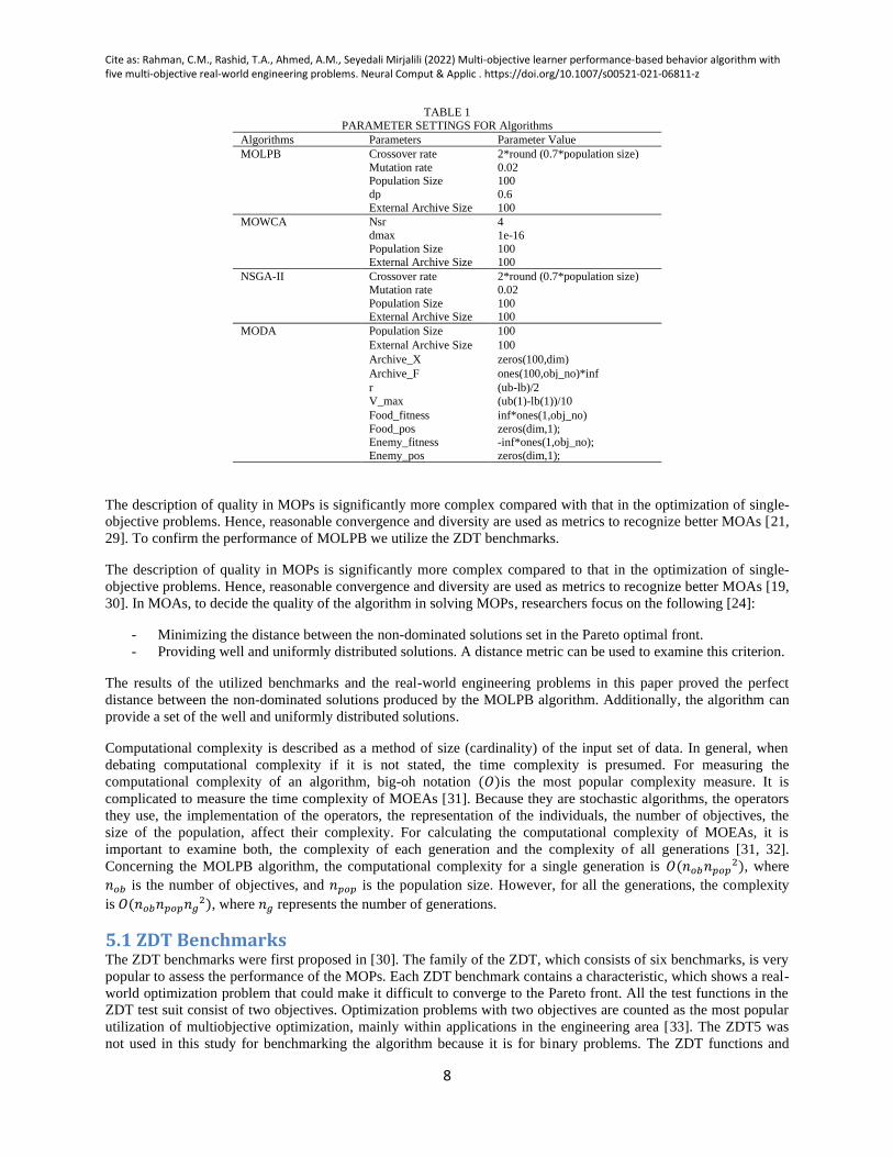
algorithms in the literature (MOWCA, NSGA-II, and MODA). The overall parameters for the MOLPB and other
participated algorithms are shown in Table 1. The parameters and MATLAB code of MOWCA, NSGA-II, and
MODA are from [26], [27], and [28], respectively. However, some of their main parameters are presented in Table
1.
MATLAB programming software was used to code the MOLPB algorithm. For optimizing each benchmark, 30
independent runs were utilized, the algorithm executed over 30 independent runs and 350 iterations each. To store
the non-dominated solutions we utilized an external archive with the size of 100. A standard laptop with a processor
Intel Core i7, 16 GHz was used. Similarly, the same conditions and computing platform are utilized to run all other
participated algorithms (MOWCA, NSGA-II, and MODA) in this paper by the authors of the work.
Cite as: Rahman, C.M., Rashid, T.A., Ahmed, A.M., Seyedali Mirjalili (2022) Multi-objective learner performance-based behavior algorithm with five multi-objective real-world engineering problems. Neural Comput & Applic . https://doi.org/10.1007/s00521-021-06811-z
8
TABLE 1 PARAMETER SETTINGS FOR Algorithms
Algorithms Parameters Parameter Value
MOLPB Crossover rate 2*round (0.7*population size)
Mutation rate 0.02 Population Size 100
dp 0.6
External Archive Size 100
MOWCA Nsr 4
dmax 1e-16
Population Size 100 External Archive Size 100
NSGA-II Crossover rate 2*round (0.7*population size)
Mutation rate 0.02
Population Size 100 External Archive Size 100
MODA Population Size 100
External Archive Size 100
Archive_X zeros(100,dim)
Archive_F ones(100,obj_no)*inf
r
V_max
(ub-lb)/2
(ub(1)-lb(1))/10
Food_fitness
Food_pos Enemy_fitness
Enemy_pos
inf*ones(1,obj_no)
zeros(dim,1); -inf*ones(1,obj_no);
zeros(dim,1);
The description of quality in MOPs is significantly more complex compared with that in the optimization of single-
objective problems. Hence, reasonable convergence and diversity are used as metrics to recognize better MOAs [21,
29]. To confirm the performance of MOLPB we utilize the ZDT benchmarks.
The description of quality in MOPs is significantly more complex compared to that in the optimization of single-
objective problems. Hence, reasonable convergence and diversity are used as metrics to recognize better MOAs [19,
30]. In MOAs, to decide the quality of the algorithm in solving MOPs, researchers focus on the following [24]:
- Minimizing the distance between the non-dominated solutions set in the Pareto optimal front.
- Providing well and uniformly distributed solutions. A distance metric can be used to examine this criterion.
The results of the utilized benchmarks and the real-world engineering problems in this paper proved the perfect
distance between the non-dominated solutions produced by the MOLPB algorithm. Additionally, the algorithm can
provide a set of the well and uniformly distributed solutions.
Computational complexity is described as a method of size (cardinality) of the input set of data. In general, when
debating computational complexity if it is not stated, the time complexity is presumed. For measuring the
computational complexity of an algorithm, big-oh notation (𝑂)is the most popular complexity measure. It is
complicated to measure the time complexity of MOEAs [31]. Because they are stochastic algorithms, the operators
they use, the implementation of the operators, the representation of the individuals, the number of objectives, the
size of the population, affect their complexity. For calculating the computational complexity of MOEAs, it is
important to examine both, the complexity of each generation and the complexity of all generations [31, 32].
Concerning the MOLPB algorithm, the computational complexity for a single generation is 𝑂(𝑛𝑜𝑏𝑛𝑝𝑜𝑝2), where
𝑛𝑜𝑏 is the number of objectives, and 𝑛𝑝𝑜𝑝 is the population size. However, for all the generations, the complexity
is 𝑂(𝑛𝑜𝑏𝑛𝑝𝑜𝑝𝑛𝑔2), where 𝑛𝑔 represents the number of generations.
5.1 ZDT Benchmarks The ZDT benchmarks were first proposed in [30]. The family of the ZDT, which consists of six benchmarks, is very
popular to assess the performance of the MOPs. Each ZDT benchmark contains a characteristic, which shows a real-
world optimization problem that could make it difficult to converge to the Pareto front. All the test functions in the
ZDT test suit consist of two objectives. Optimization problems with two objectives are counted as the most popular
utilization of multiobjective optimization, mainly within applications in the engineering area [33]. The ZDT5 was
not used in this study for benchmarking the algorithm because it is for binary problems. The ZDT functions and
Cite as: Rahman, C.M., Rashid, T.A., Ahmed, A.M., Seyedali Mirjalili (2022) Multi-objective learner performance-based behavior algorithm with five multi-objective real-world engineering problems. Neural Comput & Applic . https://doi.org/10.1007/s00521-021-06811-z
9
their parameters are presented in Table A1 in Appendix A. More information about the ZDT family test suit can be
found in [30]. The average and standard deviation for each of the ZDT benchmarks are counted for all the utilized
metrics (GD, MS, RGD, and S), and they are shown as (Ave.GD, Ave.MS, Ave.RGD, Ave.S) and (Std.GD, Std.MS,
Std.RGD, Std.S), respectively.
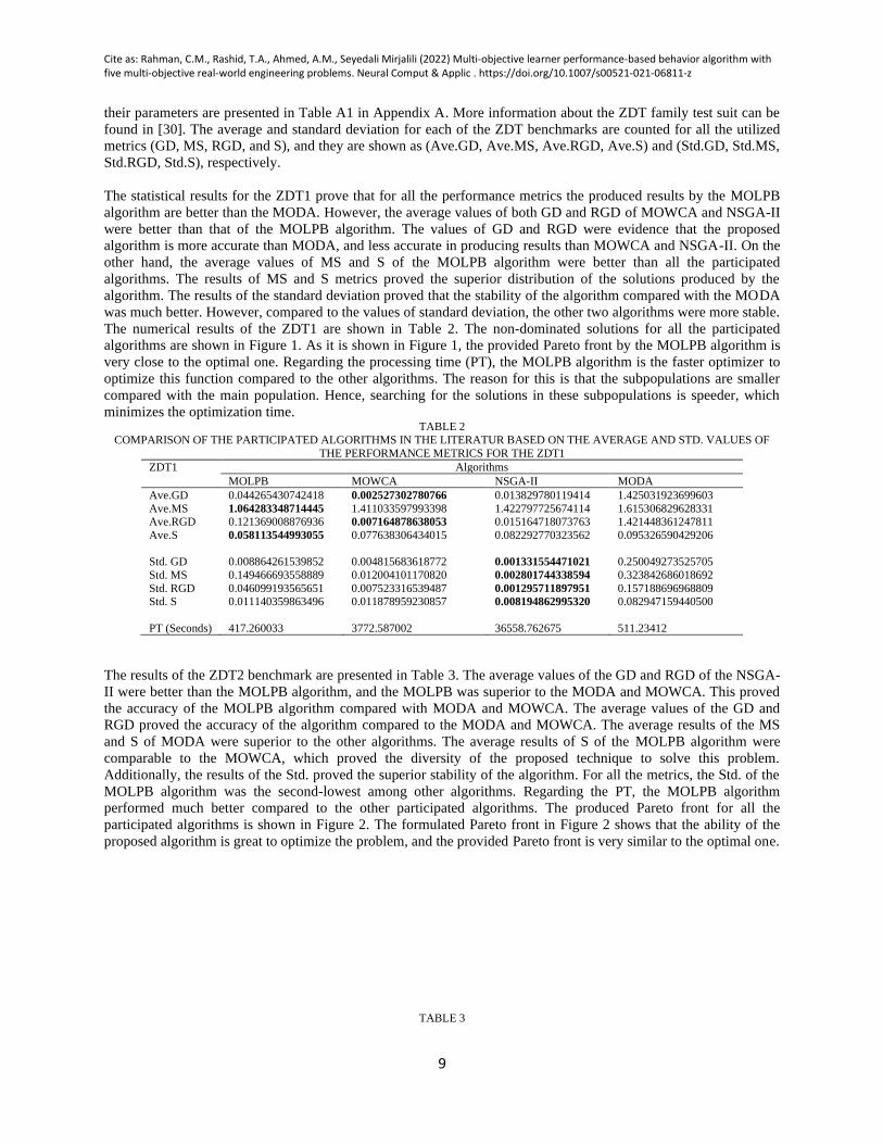
The statistical results for the ZDT1 prove that for all the performance metrics the produced results by the MOLPB
algorithm are better than the MODA. However, the average values of both GD and RGD of MOWCA and NSGA-II
were better than that of the MOLPB algorithm. The values of GD and RGD were evidence that the proposed
algorithm is more accurate than MODA, and less accurate in producing results than MOWCA and NSGA-II. On the
other hand, the average values of MS and S of the MOLPB algorithm were better than all the participated
algorithms. The results of MS and S metrics proved the superior distribution of the solutions produced by the
algorithm. The results of the standard deviation proved that the stability of the algorithm compared with the MODA
was much better. However, compared to the values of standard deviation, the other two algorithms were more stable.
The numerical results of the ZDT1 are shown in Table 2. The non-dominated solutions for all the participated
algorithms are shown in Figure 1. As it is shown in Figure 1, the provided Pareto front by the MOLPB algorithm is
very close to the optimal one. Regarding the processing time (PT), the MOLPB algorithm is the faster optimizer to
optimize this function compared to the other algorithms. The reason for this is that the subpopulations are smaller
compared with the main population. Hence, searching for the solutions in these subpopulations is speeder, which
minimizes the optimization time. TABLE 2
COMPARISON OF THE PARTICIPATED ALGORITHMS IN THE LITERATUR BASED ON THE AVERAGE AND STD. VALUES OF
THE PERFORMANCE METRICS FOR THE ZDT1
ZDT1 Algorithms
MOLPB MOWCA NSGA-II MODA
Ave.GD 0.044265430742418 0.002527302780766 0.013829780119414 1.425031923699603
Ave.MS 1.064283348714445 1.411033597993398 1.422797725674114 1.615306829628331 Ave.RGD 0.121369008876936 0.007164878638053 0.015164718073763 1.421448361247811
Ave.S 0.058113544993055 0.077638306434015 0.082292770323562 0.095326590429206
Std. GD 0.008864261539852 0.004815683618772 0.001331554471021 0.250049273525705
Std. MS 0.149466693558889 0.012004101170820 0.002801744338594 0.323842686018692
Std. RGD 0.046099193565651 0.007523316539487 0.001295711897951 0.157188696968809
Std. S 0.011140359863496 0.011878959230857
0.008194862995320
0.082947159440500
PT (Seconds) 417.260033 3772.587002 36558.762675 511.23412
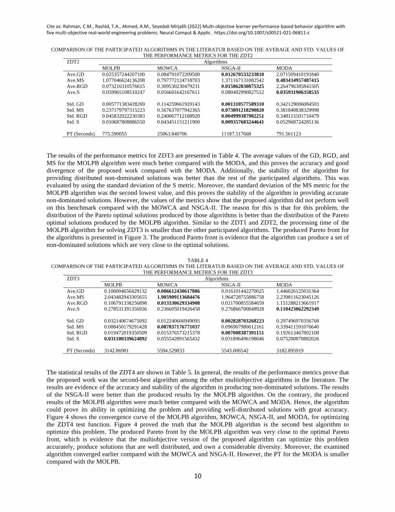
The results of the ZDT2 benchmark are presented in Table 3. The average values of the GD and RGD of the NSGA-
II were better than the MOLPB algorithm, and the MOLPB was superior to the MODA and MOWCA. This proved
the accuracy of the MOLPB algorithm compared with MODA and MOWCA. The average values of the GD and
RGD proved the accuracy of the algorithm compared to the MODA and MOWCA. The average results of the MS
and S of MODA were superior to the other algorithms. The average results of S of the MOLPB algorithm were
comparable to the MOWCA, which proved the diversity of the proposed technique to solve this problem.
Additionally, the results of the Std. proved the superior stability of the algorithm. For all the metrics, the Std. of the
MOLPB algorithm was the second-lowest among other algorithms. Regarding the PT, the MOLPB algorithm
performed much better compared to the other participated algorithms. The produced Pareto front for all the
participated algorithms is shown in Figure 2. The formulated Pareto front in Figure 2 shows that the ability of the
proposed algorithm is great to optimize the problem, and the provided Pareto front is very similar to the optimal one.
TABLE 3
Cite as: Rahman, C.M., Rashid, T.A., Ahmed, A.M., Seyedali Mirjalili (2022) Multi-objective learner performance-based behavior algorithm with five multi-objective real-world engineering problems. Neural Comput & Applic . https://doi.org/10.1007/s00521-021-06811-z
10
COMPARISON OF THE PARTICIPATED ALGORITHMS IN THE LITERATUR BASED ON THE AVERAGE AND STD. VALUES OF THE PERFORMANCE METRICS FOR THE ZDT2
ZDT2 Algorithms
MOLPB MOWCA NSGA-II MODA
Ave.GD 0.025357244207100 0.084791072209500 0.012670533233810 2.071509410191840 Ave.MS 1.077046624136208 0.797772124718703 1.371167131082542 0.483434957487415
Ave.RGD 0.073216310576615 0.309530230479231 0.015862830875325 2.264796385841505
Ave.S 0.059965108510247 0.056601642167611 0.080402990827512 0.035931906358535
Std. GD 0.005771383428269 0.114259661920143 0.001310577589310 0.342129006084503
Std. MS 0.237179797315223 0.567637077942365 0.073891218290820 0.381840838329998 Std. RGD 0.045832022230383 0.240067712168920 0.004999387982251 0.348115501710479
Std. S 0.010687808886550 0.043451151211900
0.009357683244641
0.052968724285136
PT (Seconds) 775.590055 25063.840706 11187.517668 791.561123
The results of the performance metrics for ZDT3 are presented in Table 4. The average values of the GD, RGD, and
MS for the MOLPB algorithm were much better compared with the MODA, and this proves the accuracy and good
divergence of the proposed work compared with the MODA. Additionally, the stability of the algorithm for
providing distributed non-dominated solutions was better than the rest of the participated algorithms. This was
evaluated by using the standard deviation of the S metric. Moreover, the standard deviation of the MS metric for the
MOLPB algorithm was the second lowest value, and this proves the stability of the algorithm in providing accurate
non-dominated solutions. However, the values of the metrics show that the proposed algorithm did not perform well
on this benchmark compared with the MOWCA and NSGA-II. The reason for this is that for this problem, the
distribution of the Pareto optimal solutions produced by those algorithms is better than the distribution of the Pareto
optimal solutions produced by the MOLPB algorithm. Similar to the ZDT1 and ZDT2, the processing time of the
MOLPB algorithm for solving ZDT3 is smaller than the other participated algorithms. The produced Pareto front for
the algorithms is presented in Figure 3. The produced Pareto front is evidence that the algorithm can produce a set of
non-dominated solutions which are very close to the optimal solutions.
TABLE 4
COMPARISON OF THE PARTICIPATED ALGORITHMS IN THE LITERATUR BASED ON THE AVERAGE AND STD. VALUES OF
THE PERFORMANCE METRICS FOR THE ZDT3
ZDT3 Algorithms
MOLPB MOWCA NSGA-II MODA
Ave.GD 0.106004656429132 0.006612430617886 0.016101442270025 1.446026125031364
Ave.MS 2.043482943305655 1.905909113684476 1.964728755886758 2.239811623045126
Ave.RGD 0.106791338256898 0.013330629334908 0.021700855584659 1.151288213661917 Ave.S 0.278531391356936 0.236605019426458 0.276866700848928 0.110423062292349
Std. GD 0.032140674675092 0.012240666949095 0.002828703268223 0.297496970356768 Std. MS 0.088450179291428 0.087837176771037 0.096907980612161 0.339411591076640
Std. RGD 0.019472019350509 0.015376573215378 0.007008387391151 0.192613467802108
Std. S 0.031100339624892 0.055542891565432
0.031896496198046
0.075200870882026
PT (Seconds) 3142.86981 5594.529833 5543.006542 3182.895919
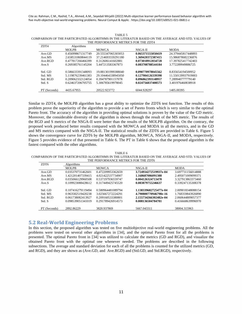
The statistical results of the ZDT4 are shown in Table 5. In general, the results of the performance metrics prove that
the proposed work was the second-best algorithm among the other multiobjective algorithms in the literature. The
results are evidence of the accuracy and stability of the algorithm in producing non-dominated solutions. The results
of the NSGA-II were better than the produced results by the MOLPB algorithm. On the contrary, the produced
results of the MOLPB algorithm were much better compared with the MOWCA and MODA. Hence, the algorithm
could prove its ability in optimizing the problem and providing well-distributed solutions with great accuracy.
Figure 4 shows the convergence curve of the MOLPB algorithm, MOWCA, NSGA-II, and MODA, for optimizing
the ZDT4 test function. Figure 4 proved the truth that the MOLPB algorithm is the second best algorithm to
optimize this problem. The produced Pareto front by the MOLPB algorithm was very close to the optimal Pareto
front, which is evidence that the multiobjective version of the proposed algorithm can optimize this problem
accurately, produce solutions that are well distributed, and own a considerable diversity. Moreover, the examined
algorithm converged earlier compared with the MOWCA and NSGA-II. However, the PT for the MODA is smaller
compared with the MOLPB.
Cite as: Rahman, C.M., Rashid, T.A., Ahmed, A.M., Seyedali Mirjalili (2022) Multi-objective learner performance-based behavior algorithm with five multi-objective real-world engineering problems. Neural Comput & Applic . https://doi.org/10.1007/s00521-021-06811-z
11
TABLE 5
COMPARISON OF THE PARTICIPATED ALGORITHMS IN THE LITERATUR BASED ON THE AVERAGE AND STD. VALUES OF
THE PERFORMANCE METRICS FOR THE ZDT4
ZDT4 Algorithms MOLPB MOWCA NSGA-II MODA
Ave.GD 0.456998671317749 20.555347065303053 0.065371555050419 24.379445817448893
Ave.MS 2.658531869844119 37.214693559291180 1.369420372387415 15.986878682236876 Ave.RGD 0.477817266466399 0.312606141602881 0.073018912034728 17.397825417742403
Ave.S 0.269385761145204 5.447213583367873 0.083708788544184 3.772289949886725
Std. GD 0.586633391348093 19.881301999388040 0.090770978045562 8.835654194500952
Std. MS 5.119876239461383 29.104464338945050 0.127984126339398 11.550139937919003
Std. RGD 0.209062332124054 0.394787901157078 0.096862393148957 7.289940777779140 Std. S 0.624637206705755 5.306785619978045
0.024756837408573 3.401976460838918
PT (Seconds) 4435.67955 20522.923772 6044.928297 1405.00395
Similar to ZDT4, the MOLPB algorithm has a great ability to optimize the ZDT6 test function. The results of this
problem prove the superiority of the algorithm to provide a set of Pareto fronts which is very similar to the optimal
Pareto front. The accuracy of the algorithm in providing optimal solutions is proven by the value of the GD metric.
Moreover, the considerable diversity of the algorithm is shown through the result of the MS metric. The results of
the RGD and S metrics of the NSGA-II were better than the results of the MOLPB algorithm. On the contrary, the
proposed work produced better results compared with the MOWCA and MODA in all the metrics, and in the GD
and MS metrics compared with the NSGA-II. The statistical results of the ZDT6 are provided in Table 6. Figure 5
shows the convergence curve for ZDT6 by the MOLPB algorithm, MOWCA, NSGA-II, and MODA, respectively.
Figure 5 provides evidence of that presented in Table 6. The PT in Table 6 shows that the proposed algorithm is the
fastest compared with the other algorithms.
TABLE 6
COMPARISON OF THE PARTICIPATED ALGORITHMS IN THE LITERATUR BASED ON THE AVERAGE AND STD. VALUES OF
THE PERFORMANCE METRICS FOR THE ZDT6
ZDT6 Algorithms
MOLPB MOWCA NSGA-II MODA
Ave.GD 0.035370731462601 0.472209953362659 3.724934272519937e-04 3.697731156014888
Ave.MS 1.421201407339415 4.021422537734907 1.168687086091388 2.495071009099371 Ave.RGD 0.035066129960508 0.537197936559747 0.004126324713478 3.327913863373460
Ave.S 0.109923088428612 0.317449425745520 0.083879755246637 0.339247135308378
Std. GD 0.107416279119494 0.580964481089794 1.138339682725477e-04 2.009018348088154
Std. MS 0.963582519420238 3.025667272224291 4.790800770946798e-16 1.768359843926890
Std. RGD 0.061738082413927 0.209160533380801 2.155734266302482e-04 2.060644809057377 Std. S 0.098539051341019 0.291789426914573
0.008136504784781 0.416668639996970
PT (Seconds) 2892.86229 3820.937869 5667.043311 38004.315963
5.2 Real-World Engineering Problems In this section, the proposed algorithm was tested on five multiobjective real-world engineering problems. All the
problems were tested on several other algorithms in [34], and the optimal Pareto front for all the problems is
presented. The optimal Pareto front in [34] was utilized to calculate the metrics (GD and RGD), and visualize the
obtained Pareto front with the optimal one whenever needed. The problems are described in the following
subsections. The average and standard deviation for each of all the problems is counted for the utilized metrics (GD,
and RGD), and they are shown as (Ave.GD, and Ave.RGD) and (Std.GD, and Std.RGD), respectively.
Cite as: Rahman, C.M., Rashid, T.A., Ahmed, A.M., Seyedali Mirjalili (2022) Multi-objective learner performance-based behavior algorithm with five multi-objective real-world engineering problems. Neural Comput & Applic . https://doi.org/10.1007/s00521-021-06811-z
12
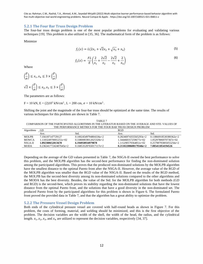
5.2.1 The Four Bar Truss Design Problem The four-bar truss design problem is one of the most popular problems for evaluating and validating various
techniques [19]. This problem is also utilized in [35, 36]. The mathematical form of the problem is as follows:
Minimize
𝑓1(𝑥) = 𝐿(2𝑥1 + √2𝑥2 + √𝑥3 + 𝑥4) (5)
𝑓2(𝑥) = 𝐹𝐿
𝐸(
2
𝑥1
+2√2
𝑥2
−2√2
𝑥3
+2
𝑥4
) (6)
Where
(𝐹
𝜎) ≤ 𝑥1, 𝑥4 ≤ 3 × (
𝐹
𝜎)
√2 × (𝐹
𝜎) ≤ 𝑥2, 𝑥3 ≤ 3 × (
𝐹
𝜎)
The parameters are as follows:
F = 10 kN, E = (2)105 kN/cm2 , L = 200 cm, 𝜎 = 10 kN/cm3 .
Shifting the joint and the magnitude of the four-bar truss should be optimized at the same time. The results of
various techniques for this problem are shown in Table 7.
TABLE 7
COMPARISON OF THE PARTICIPATED ALGORITHMS IN THE LITERATUR BASED ON THE AVERAGE AND STD. VALUES OF
THE PERFORMANCE METRICS FOR THE FOUR BAR TRUSS DESIGN PROBLEM
Algorithms GD RGD
Ave. Std. Ave. Std.
MOLPB 7.356187147729127 0.10024549794804336e+2 0.28246974355565293e+2 0.13866918530380362e+2
MOWCA 1.118324970001251e+02 0.33800859012025320e+2 1.344468357259677e+02 1.052978069707367e+02 NSGA-II 1.892380652813678 6.194958934979878 1.115290579364851e+02 0.25798795805055256e+2
MODA 0.23634177242407645e+2 0.16853528765017117e+2 0.21102208608179346e+2 7.085411854194526
Depending on the average of the GD values presented in Table 7, the NSGA-II owned the best performance to solve
this problem, and the MOLPB algorithm has the second-best performance for finding the non-dominated solution
among the participated algorithms. This proves that the produced non-dominated solutions by the MOLPB algorithm
have the smallest distance to the optimal Pareto front after the NSGA-II. However, the average value of the RGD of
the MOLPB algorithm was smaller than the RGD value of the NSGA-II. Based on the results of the RGD method,
the MOLPB has the second-best diversity among its non-dominated solutions compared to the other algorithms and
the MODA has the best diversity. Besides, the value of the Std. for the MOLPB algorithm for both methods (GD
and RGD) is the second-best, which proves its stability regarding the non-dominated solutions that have the lowest
distance from the optimal Pareto front, and the solutions that have a good diversity in the non-dominated set. The
produced Pareto front by the participated algorithms for this problem is shown in Figure 6. The formulated Pareto
front proved the provided data in Table 7, and that the algorithm has a great ability to optimize the problem.
5.2.2 The Pressure Vessel Design Problem Both ends of the cylindrical pressure vessel are covered with half-round heads as shown in Figure 7. For this
problem, the costs of forming, material, and welding should be minimized, and this is the first objective of the
problem. The decision variables are the width of the shell, the width of the head, the radius, and the cylindrical
length. 𝑥1, 𝑥2, 𝑥3, and 𝑥4 are utilized to represent the decision variables, respectively [34, 37].
Cite as: Rahman, C.M., Rashid, T.A., Ahmed, A.M., Seyedali Mirjalili (2022) Multi-objective learner performance-based behavior algorithm with five multi-objective real-world engineering problems. Neural Comput & Applic . https://doi.org/10.1007/s00521-021-06811-z
13
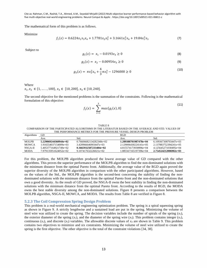
The mathematical form of this problem is as follows.
Minimize
𝑓1(𝑥) = 0.6224𝑥1𝑥3𝑥4 + 1.7781𝑥2𝑥32 + 3.1661𝑥1
2𝑥4 + 19.84𝑥12𝑥3
(7)
Subject to
𝑔1(𝑥) = 𝑥1 − 0.0193𝑥3 ≥ 0
(8)
𝑔2(𝑥) = 𝑥2 − 0.00954𝑥3 ≥ 0
(9)
𝑔3(𝑥) = 𝜋𝑥3
2𝑥4 +4
3𝜋𝑥3
3 − 1296000 ≥ 0
(10)
Where
𝑥1, 𝑥2 ∈ {1, … . . , 100}, 𝑥3 ∈ [10, 200], 𝑥4 ∈ [10, 240].
The second objective for the mentioned problems is the summation of the constraints. Following is the mathematical
formulation of this objective:
𝑓2(𝑥) = ∑ 𝑚𝑎𝑥{𝑔𝑖(𝑥), 0}
3
𝑖=1
(11)
TABLE 8
COMPARISON OF THE PARTICIPATED ALGORITHMS IN THE LITERATUR BASED ON THE AVERAGE AND STD. VALUES OF THE PERFORMANCE METRICS FOR THE PRESSURE VESSEL DESIGN PROBLEM
Algorithms GD RGD
Ave. Std. Ave. Std.
MOLPB 5.229069244360944e+02 0.76606682134282340e+02 1.289388701987478e+04 6.109367308703447e+03 MOWCA 1.916554037154009e+03 3.420966646903447e+03 2.129006430224141e+05 2.137883752394241e+05
NSGA-II 5.405377164921749e+02 0.3665932587233484e+02 4.815574173930896e+04 4.125645271030495e+04
MODA 7.979135951624052e+02 9.107417632226021e+02 1.885567165197396e+04 2.754524212006902e+03
For this problem, the MOLPB algorithm produced the lowest average value of GD compared with the other
algorithms. This proves the superior performance of the MOLPB algorithm to find the non-dominated solutions with
the minimum distance from the optimal Pareto front. Additionally, the average value of the RGD again proved the
superior diversity of the MOLPB algorithm in comparison with the other participated algorithms. However, based
on the values of the Std., the MOLPB algorithm is the second-best concerning the stability of finding the non-
dominated solutions with the minimum distance from the optimal Pareto front and the non-dominated solutions that
own a good diversity. As the result of GD proved, the NSGA-II owns the best stability in finding the non-dominated
solutions with the minimum distance from the optimal Pareto front. According to the results of RGD, the MODA
owns the best stable diversity among the non-dominated solutions. Figure 8 presents a comparison between the
MOLPB algorithm, NSGA-II, MOWCA, and MODA. The results from Table 8 are verified in Figure 8.
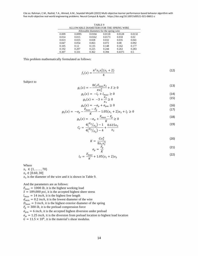
5.2.3 The Coil Compression Spring Design Problem This problem is a real-world mechanical engineering optimization problem. The spring is a spiral squeezing spring
as shown in Figure 9. A strictly lengthwise and a sustained load are put in the spring. Minimizing the volume of
steel wire was utilized to create the spring. The decision variables include the number of spirals of the spring (x1),
the exterior diameter of the spring (x2), and the diameter of the spring wire (x3). This problem contains integer (x1),
continuous (x2), and discrete (x3) variables. The allowable discrete values of x3 are shown in Table 9. This problem
contains two objectives to minimize and six constraints. Minimizing the volume of steel wire utilized to create the
spring is the first objective. The other objective is the total of the constraint violations [34, 38].
Cite as: Rahman, C.M., Rashid, T.A., Ahmed, A.M., Seyedali Mirjalili (2022) Multi-objective learner performance-based behavior algorithm with five multi-objective real-world engineering problems. Neural Comput & Applic . https://doi.org/10.1007/s00521-021-06811-z
14
TABLE 9 ALLOWABLE DIAMETERS FOR THE SPRING WIRE
Allowable diameters for the spring wire
0.009 0.0095 0.0104 0.0118 0.0128 0.0132
0.014 0.015 0.0162 0.0173 0.018 0.02 0.023 0.025 0.028 0.032 0.035 0.041
0.047 0.054 0.063 0.072 0.08 0.092
0.105 0.12 0.135 0.148 0.162 0.177 0.192 0.207 0.225 0.244 0.263 0.283
0.307 0.331 0.362 0.394 0.4375 0.5
This problem mathematically formulated as follows:
𝑓1(𝑥) =
𝜋2𝑥2𝑥32(𝑥1 + 2)
4
(12)
Subject to
𝑔1(𝑥) = −
8𝐶𝑓𝐹𝑚𝑎𝑥𝑥2
𝜋𝑥33 + 𝑆 ≥ 0
(13)
𝑔2(𝑥) = −𝑙𝑓 + 𝑙𝑚𝑎𝑥 ≥ 0 (14)
𝑔3(𝑥) = −3 +𝑥2
𝑥3
≥ 0 (15)
𝑔4(𝑥) = −𝜎𝑝 + 𝜎𝑝𝑚 ≥ 0 (16)
𝑔5(𝑥) = −𝜎𝑝 −
𝐹𝑚𝑎𝑥 − 𝐹𝑝
𝐾− 1.05(𝑥1 + 2)𝑥3 + 𝑙𝑓 ≥ 0
(17)
𝑔6(𝑥) = −𝜎𝑤 +
𝐹𝑚𝑎𝑥 − 𝐹𝑝
𝐾≥ 0
(18)
𝐶𝑓 =
4(𝑥2
𝑥3⁄ ) − 1
4(𝑥2
𝑥3⁄ ) − 4
+0.615𝑥3
𝑥2
(19)
𝐾 =
𝐺𝑥34
8𝑥1𝑥23
(20)
𝜎𝑝 =
𝐹𝑝
𝐾
(21)
𝑙𝐹 =
𝐹𝑚𝑎𝑥
𝐾+ 1.05(𝑥1 + 2)𝑥3
(22)
Where
𝑥1 ∈ {1, … … , 70}
𝑥2 ∈ [0.60, 30] 𝑥3 is the diameter of the wire and it is shown in Table 9.
And the parameters are as follows:
𝐹𝑚𝑎𝑥 = 1000 𝑙𝑏, it is the highest working load
𝑆 = 189,000 𝑝𝑠𝑖, it is the accepted highest sheer stress
𝑙𝑚𝑎𝑥 = 14 𝑖𝑛𝑐ℎ, it is the highest free length
𝑑𝑚𝑖𝑛 = 0.2 𝑖𝑛𝑐ℎ, it is the lowest diameter of the wire
𝐷𝑚𝑎𝑥 = 3 𝑖𝑛𝑐ℎ, it is the highest exterior diameter of the spring
𝐹𝑝 = 300 𝑙𝑏, it is the preload compression force
𝜎𝑝𝑚 = 6 𝑖𝑛𝑐ℎ, it is the accepted highest diversion under preload
𝜎𝑤 = 1.25 𝑖𝑛𝑐ℎ, it is the diversion from preload location to highest load location
𝐺 = 11.5 × 10⁶, it is the material’s shear modulus.
Cite as: Rahman, C.M., Rashid, T.A., Ahmed, A.M., Seyedali Mirjalili (2022) Multi-objective learner performance-based behavior algorithm with five multi-objective real-world engineering problems. Neural Comput & Applic . https://doi.org/10.1007/s00521-021-06811-z
15
𝑓2(𝑥) = ∑ 𝑚𝑎𝑥{𝑔𝑖(𝑥), 0}
6
𝑖=1
(23)
The produced results in Table 10 show that the MOLPB algorithm outperforms other participated algorithms to
solve the coil compression spring design problem. The proposed algorithm produced the minimum average result for
both the GD and RGD methods. These produced results for the GD technique is evidence for the superior
performance of the MOLPB algorithm to find the non-dominated solutions with the smallest distance from the
optimal Pareto front. Moreover, the lowest average result for the RGD proved the superior diversity of the proposed
algorithm. Additionally, the minimum result of the std. for the MOLPB algorithm compared with the other
algorithms showed the stability of the algorithm. Figure 10 proved the results shown in Table 10.
TABLE 10
COMPARISON OF THE PARTICIPATED ALGORITHMS IN THE LITERATUR BASED ON THE AVERAGE AND STD. VALUES OF
THE PERFORMANCE METRICS FOR THE COIL COMPRESSION SPRING DESIGN PROBLEM Algorithms GD RGD
Ave. Std. Ave. Std.
MOLPB 0.001165137348271 5.953683716862298e-04 3.907638898625130e+02 6.995757373604563e+02 MOWCA 0.036219782034087 0.162110588997669 4.782498529340439e+04 1.086536014708315e+05
NSGA-II 1.766560342824665e+02 6.683175803097043e+02 3.579777017698174e+03 6.631512913748524e+03
MODA 1.468585635356069e+04 2.764022957116235e+04 3.579274283635858e+03 2.297668234226298e+03
5.2.4 The Speed Reducer Design Problem This problem was first designed as a single objective optimization problem. It was then converted to many-objective
optimization. It is the design of a gearbox that can be utilized in some airplanes. It contains three objectives, eleven
constraints, and seven decision variables. The first two objectives of the problem are to reduce the volume and the
stress in either of the gear shafts, respectively. The third objective is the total of the constraints. This problem is also
utilized to test other algorithms in [34, 36, 39]. The mathematical formulation of the problem is as follows:
𝑓1(𝑥) = 0.7854𝑥1𝑥2
2 (10𝑥3
2
3+ 14.933𝑥3 − 43.0934)
−1.508𝑥1(𝑥62 + 𝑥7
2) + 7.477(𝑥63 + 𝑥7
3)
+0.7854(𝑥4𝑥62 + 𝑥5𝑥7
2)
(24)
𝑓2(𝑥) = √(
745𝑥4𝑥2𝑥3
⁄ )2
+ 1.69 × 10⁷
0.1𝑥63
(25)
𝑔1(𝑥) =
1
27−
1
𝑥1𝑥23𝑥3
≥ 0 (26)
𝑔2(𝑥) =
1
397.5−
1
𝑥1𝑥22𝑥3
2 ≥ 0 (27)
𝑔3(𝑥) =
1
1.92−
𝑥43
𝑥2𝑥3𝑥64 ≥ 0
(28)
𝑔4(𝑥) =
1
1.93−
𝑥53
𝑥2𝑥3𝑥74 ≥ 0
(29)
𝑔5(𝑥) = 40 − 𝑥2𝑥3 ≥ 0 (30)
𝑔6(𝑥) = 12 −𝑥1
𝑥2
≥ 0 (31)
𝑔7(𝑥) = −5 +𝑥1
𝑥2
≥ 0 (32)
𝑔8(𝑥) = −1.9 + 𝑥4 − 1.6𝑥6 ≥ 0 (33)
Cite as: Rahman, C.M., Rashid, T.A., Ahmed, A.M., Seyedali Mirjalili (2022) Multi-objective learner performance-based behavior algorithm with five multi-objective real-world engineering problems. Neural Comput & Applic . https://doi.org/10.1007/s00521-021-06811-z
16
𝑔9(𝑥) = −1.9 + 𝑥5 − 1.1𝑥7 ≥ 0 (34)
𝑔10(𝑥) = 1300 − 𝑓2(𝑥) ≥ 0 (35)
𝑔11(𝑥) = 1100 −√(
745𝑥5𝑥2𝑥3
⁄ )2
+ 1.575 × 10⁸
0.1𝑥73 ≥ 0
(36)
Where
𝑥1 ∈ [2.6, 3.6], it indicates the width of the gear face. 𝑥2 ∈ [0.7, 0.8], it is the module of the teeth. 𝑥3 ∈{17, … . , 28}, it indicates the number of teeth in the gear. 𝑥4 ∈ [7.8, 8.3], it is the space among the bearings on the
first cylinder. 𝑥5 ∈ [7.8, 8.3], it is the space among the bearings on the second cylinder. 𝑥6 ∈ [2.9, 3.9], and 𝑥7 ∈[5, 5.5], are the diameters of the first and second cylinders, respectively.
The third objective is the total of all the constraints, as follows:
𝑓3 = ∑ 𝑚𝑎𝑥{𝑔𝑖(𝑥), 0}
11
𝑖=1
(37)
In general, the results in Table 11 show that MOLPB was the second-best algorithm to solve this problem. The
NSGA-II produced the smallest value for the GD method. Comparing to the rest of the algorithms in this work, the
MOLPB algorithm produced the minimum average value of the GD technique. This proves the superiority of both
NSGA-II and MOLPB to find the non-dominated solutions with the smallest distance from the optimal Pareto front.
Additionally, the superiority of the proposed algorithm was proved for finding non-dominated solutions that have
good diversity. The result of the RGD method is reasonable evidence for the superior diversity of the algorithm.
Moreover, the results of the Std. showed the stability of the MOLPB algorithm to solve the problem. Figure 11
shows the produced Pareto front by the participated algorithms. The formulated Pareto front is evident to that
provided in Table 11.
TABLE 11
COMPARISON OF THE PARTICIPATED ALGORITHMS IN THE LITERATUR BASED ON THE AVERAGE AND STD. VALUES OF
THE PERFORMANCE METRICS FOR THE SPEED REDUCER DESIGN PROBLEM Algorithms GD RGD
Ave. Std. Ave. Std.
MOLPB 0.11300957429052747e+02 5.353901079223076 4.417567589123142e+02 1.204597287830257e+02 MOWCA 0.12093211543779878e+02 8.095693487854756 4.706728443589605e+02 3.351003926974380e+02
NSGA-II 9.248983587521442 4.355702417490958 8.757171216956020e+02 1.433600470583269e+02 MODA 0.48368624551698005e+02 0.27723667813065873e+02 1.259847489533345e+02 0.757966829513193e+02
5.2.5 The Car Side Impact Design Problem This problem was also addressed in [34, 40, 41]. It consists of four objectives. The aim of the first three objectives
(𝑓1, 𝑓2, and 𝑓3) is reduce the heaviness of the car, the pubic force that passengers went through, and the V-pillar’s
total velocity which is in charge of resisting the impact load, respectively. The original problem consists of eleven
decision variables. However, since we use the problem from [34], the four stochastic variables are excluded. The
formulation of the problem is as follows:
𝑓1(𝑥) = 1.98 + 4.9𝑥1 + 6.67𝑥2 + 6.98𝑥3 + 4.01𝑥4 + 1.78𝑥5 + 10−5𝑥6 + 2.73𝑥7
(38)
𝑓2(𝑥) = 4.72 − 0.5𝑥4 − 0.19𝑥2𝑥3 (39)
𝑓3(𝑥) = 0.5(𝑉𝑀𝐵𝑃(𝑥) + 𝑉𝐹𝐷(𝑥)) (40)
𝑔1(𝑥) = 1 − 1.16 + 0.3717𝑥2𝑥4 + 0.0092928𝑥3 ≥ 0
(41)
Cite as: Rahman, C.M., Rashid, T.A., Ahmed, A.M., Seyedali Mirjalili (2022) Multi-objective learner performance-based behavior algorithm with five multi-objective real-world engineering problems. Neural Comput & Applic . https://doi.org/10.1007/s00521-021-06811-z
17
𝑔2(𝑥) = 0.32 − 0.261 + 0.0159𝑥1𝑥2 + 0.06486𝑥1 +0.019𝑥2𝑥7 − 0.0144𝑥3𝑥5 − 0.0154464𝑥6 ≥ 0
(42)
𝑔3(𝑥) = 0.32 − 0.214 − 0.00817𝑥5 + 0.045195𝑥1 +0.0135168𝑥1 − 0.03099𝑥2𝑥6 + 0.018𝑥2𝑥7 − 0.007176𝑥3
−0.023232𝑥3 + 0.00364𝑥5𝑥6 + 0.018𝑥22 ≥ 0
(43)
𝑔4(𝑥) = 0.32 − 0.74 + 0.61𝑥2 + 0.031296𝑥3 + 0.031872𝑥7 − 0.227𝑥22 ≥ 0 (44)
𝑔5(𝑥) = 32 − 28.98 − 3.818𝑥3 + 4.2𝑥1𝑥2 − 1.27296𝑥6 + 2.68065𝑥7 ≥ 0
(45)
𝑔6(𝑥) = 32 − 33.86 − 2.95𝑥3 + 5.057𝑥1𝑥2 + 3.795𝑥2 + 3.4431𝑥7 − 1.45728 ≥ 0 (46)
𝑔7(𝑥) = 32 − 46.36 + 9.9𝑥2 + 4.4505𝑥1 ≥ 0 (47)
𝑔8(𝑥) = 4 − 𝑓2(𝑥) ≥ 0 (48)
𝑔9(𝑥) = 9.9 − 𝑉𝑀𝐵𝑃(𝑥) ≥ 0 (49)
𝑉𝑀𝐵𝑃(𝑥) = 10.58 − 0.674𝑥1 − 0.67275𝑥2 (50)
𝑉𝐹𝐷(𝑥) = 16.45 − 0.489𝑥3𝑥7 − 0.843𝑥5𝑥6 (51)
Where
𝑥1 ∈ [0.5, 1.5] indicates the width of B-Pillar inner, 𝑥2 ∈ [0.45, 1.35] indicates the width of B-Pillar augmentation,
𝑥3 ∈ [0.5, 1.5] indicates the width of the interior floor side, 𝑥4 ∈ [0.5, 1.5] indicates the width of cross members,
𝑥5 ∈ [0.875, 2.625] indicates the width of the door beam, 𝑥6 ∈ [0.4, 1.2] indicates the width of door augmentation,
𝑥7 ∈ [0.4, 1.2] indicates the width roof rail.
Objective number four is the total of the constraints, as follows:
𝑓4(𝑥) = ∑ 𝑚𝑎𝑥{𝑔𝑖(𝑥), 0}
10
𝑖=1
(52)
As shown in Table 12, the results show the ability of the MOLPB algorithm to solve this problem. In addition to the
high number of objective, decision variables, and constraints the proposed algorithm performed better than the other
algorithms to solve the problem. The results proved the super-diversity and performance of the algorithm. It
performed superior to produce non-dominated solutions with a small distance from the optimal Pareto front.
Additionally, it owned a good diversity and this was proved by the results of the RGD method. The small value of
the Std. showed the amazing stability of the algorithm. Moreover, the result of the GD of the MOLPB algorithm was
better compared with the other algorithms, and this proves the accuracy of the produced results by the algorithm.
Figure 12 shows the produced Pareto front by the participated algorithms. As shown, the proposed algorithm
provided a better Pareto front compared with other algorithms. This is evidence of the ability of the proposed
algorithm to optimize multiobjective problems and produce accurate results.
TABLE 12 COMPARISON OF THE PARTICIPATED ALGORITHMS IN THE LITERATUR BASED ON THE AVERAGE AND STD. VALUES OF
THE PERFORMANCE METRICS FOR THE CAR SIDE-IMPACT DESIGN PROBLEM Algorithms GD RGD
Ave. Std. Ave. Std.
MOLPB 0.303015888766268 0.030579816675289 1.567421887332045 0.285633108011381 MOWCA 3.927957536364954 0.359717355795984 8.715478788882232 0.345128037040276 NSGA-II 0.1993309223566308e+02 0.875884770917414 9.587727366029336 0.184723790431805 MODA 0.310141340133575 0.078033566503663 2.070993601511424 0.623158723216559
Cite as: Rahman, C.M., Rashid, T.A., Ahmed, A.M., Seyedali Mirjalili (2022) Multi-objective learner performance-based behavior algorithm with five multi-objective real-world engineering problems. Neural Comput & Applic . https://doi.org/10.1007/s00521-021-06811-z
18
6. Conclusions In this work, a new multiobjective algorithm called MOLPB was proposed. The MOLPB algorithm is a brand new
algorithm for solving problems that have many objectives. The basic ideas of the MOLPB algorithm were motivated
by the process of transferring graduated learners from high school to university and improving the studying
behaviors of the learners at colleges. The proposed multiobjective algorithm was utilized to optimize a group of
benchmarks, and five real-world engineering problems. To confirm the efficacy and ability of the algorithm several
criteria were utilized. The produced statistical results from the metrics are evidence that the algorithm can approach
the optimal Pareto front and produce a set of good non-dominated solutions compared with other multiobjective
algorithms in the literature. Depending on the reported results, the MOLPB algorithm, in general, provides better or
competitive results compared with the other multiobjective algorithms. However, in some cases, the NSGA-II
outperformed the proposed algorithm. However, the diversity of the algorithm almost was better than the rest of the
algorithms in the literature. Although, the MOLPB algorithm proved its ability to optimize different real-world
engineering problems and a group of benchmarks, the nature of the problem may affect the performance of the
algorithm similar to any other algorithms. In general, the proposed multiobjective algorithm is a suitable technique
to provide Pareto optimal solutions for various multiobjective optimization problems.
For future works, several research directions can be recommended. Firstly, the authors recommend utilizing the
proposed technique to optimize different problems and compare the results with other multiobjective heuristic
techniques. Additionally, proposing a new technique to utilize in the MOLPB algorithm to recognize non-dominated
solutions instead of the crowding-based technique is highly recommended.
Cite as: Rahman, C.M., Rashid, T.A., Ahmed, A.M., Seyedali Mirjalili (2022) Multi-objective learner performance-based behavior algorithm with five multi-objective real-world engineering problems. Neural Comput & Applic . https://doi.org/10.1007/s00521-021-06811-z
19
References [1] Bao, T., Gupta, P., and Mordukhovich, B., 2007. Necessary Conditions in Multiobjective Optimization with
Equilibrium Constraints. Journal of Optimization Theory and Applications, [online] 135(2), pp.179-203. Available
at: <https://link.springer.com/article/10.1007/s10957-007-9209-x> [Accessed 27 June 2020].
[2] Bao, T., and Mordukhovich, B., 2008. Necessary conditions for super minimizers in constrained multiobjective
optimization. Journal of Global Optimization, [online] 43(4), pp.533-552. Available at:
<https://dl.acm.org/doi/10.1007/s10898-008-9336-4> [Accessed 27 June 2020].
[3] Volle, M., 2010. Theorems of the Alternative for Multivalued Mappings and Applications to Mixed
Convex\Concave Systems of Inequalities. Set-Valued and Variational Analysis, [online] 18(3-4), pp.601-616.
Available at: <https://link.springer.com/article/10.1007%2Fs11228-010-0155-7> [Accessed 27 June 2020].
[4] Coello Coello, C., González Brambila, S., Figueroa Gamboa, J., Castillo Tapia, M. and Hernández Gómez, R.,
2019. Evolutionary multiobjective optimization: open research areas and some challenges lying ahead. Complex &
Intelligent Systems, [online] Available at: <https://link.springer.com/article/10.1007/s40747-019-0113-4> [Accessed
27 June 2020].
[5] Deb, K., 2008. Introduction to Evolutionary Multiobjective Optimization. Multiobjective Optimization, [online]
5252, pp.59-96. Available at: <https://link.springer.com/chapter/10.1007/978-3-540-88908-3_3> [Accessed 28 June
2020].
[6] Gunantara, N., 2018. A review of multi-objective optimization: Methods and its applications. Cogent
Engineering, [online] 5(1). Available at: <https://www.tandfonline.com/doi/full/10.1080/23311916.2018.1502242>
[Accessed 28 June 2020].
[7] Zitzler, E. and Thiele, L., 1999. Multiobjective evolutionary algorithms: a comparative case study and the
strength Pareto approach. IEEE Transactions on Evolutionary Computation, 3(4), pp.257-271.
[8] Fawaz, A., 2007. Improving Convergence, Diversity And Pertinency In Multiobjective Optimisation. Ph.D.
Sheffield.
[9] Zahoor Raja, M., Shah, Z., Anwaar Manzar, M., Ahmad, I., Awais, M. and Baleanu, D. (2018). A new stochastic
computing paradigm for nonlinear Painlevé II systems in applications of random matrix theory. The European
Physical Journal Plus, [online] 133(7). Available at: https://link.springer.com/article/10.1140/epjp/i2018-12080-4
[Accessed 10 Dec. 2019].
[10] Sabir, Z., Manzar, M., Raja, M., Sheraz, M. and Wazwaz, A. (2018). Neuro-heuristics for nonlinear singular
Thomas-Fermi systems. Applied Soft Computing, [online] 65, pp.152-169. Available at:
https://www.sciencedirect.com/science/article/abs/pii/S1568494618300152 [Accessed 10 Dec. 2019].
[11] Kang, F., Li, J. and Dai, J., 2019. Prediction of long-term temperature effect in structural health monitoring of
concrete dams using support vector machines with Jaya optimizer and salp swarm algorithms. Advances in
Engineering Software, [online] 131, pp.60-76. Available at:
<https://www.sciencedirect.com/science/article/abs/pii/S0965997818310378> [Accessed 6 March 2021].
[12] Donateo, T., Pascalis, C. and Ficarella, A., 2018. Many-Objective Optimization of Mission and Hybrid Electric
Power System of an Unmanned Aircraft. In: K. Sim and P. Kaufmann, ed., Applications of Evolutionary
Computation. [online] Parma: Springer, Cham, pp.231-246. Available at:
<https://link.springer.com/book/10.1007/978-3-319-77538-8> [Accessed 4 July 2020].
[13] Zitzler, E., Laumanns, M. and Bleuler, S., 2004. A Tutorial on Evolutionary Multiobjective
Optimization. Lecture Notes in Economics and Mathematical Systems, [online] 535, pp.3-37. Available at:
<https://link.springer.com/chapter/10.1007/978-3-642-17144-4_1> [Accessed 4 July 2020].
Cite as: Rahman, C.M., Rashid, T.A., Ahmed, A.M., Seyedali Mirjalili (2022) Multi-objective learner performance-based behavior algorithm with five multi-objective real-world engineering problems. Neural Comput & Applic . https://doi.org/10.1007/s00521-021-06811-z
20
[14] Rahman, C. and Rashid, T., 2020. A new evolutionary algorithm: Learner performance based behavior
algorithm. Egyptian Informatics Journal, [online] Available at:
<https://www.sciencedirect.com/science/article/pii/S1110866520301419> [Accessed 9 September 2020].
[15] Nebro, A., Durillo, J., Luna, F., Dorronsoro, B. and Alba, E., 2009. MOCell: A cellular genetic algorithm for
multiobjective optimization. International Journal of Intelligent Systems, [online] 24(7), pp.726-746. Available at:
<https://onlinelibrary.wiley.com/doi/abs/10.1002/int.20358> [Accessed 7 July 2020].
[16] Deb, K., Pratap, A., Agarwal, S. and Meyarivan, T., 2002. A fast and elitist multiobjective genetic algorithm:
NSGA-II. IEEE Transactions on Evolutionary Computation, [online] 6(2), pp.182-197. Available at:
<https://ieeexplore.ieee.org/document/996017> [Accessed 7 July 2020].
[17] Zitzler, E., Deb, K. and Thiele, L., 2000. Comparison of Multiobjective Evolutionary Algorithms: Empirical
Results. Evolutionary Computation, [online] 8(2), pp.173-195. Available at:
<https://dl.acm.org/doi/10.1162/106365600568202> [Accessed 7 July 2020].
[18] Zitzler, E. and Thiele, L., 1999. Multiobjective evolutionary algorithms: a comparative case study and the
strength Pareto approach. IEEE Transactions on Evolutionary Computation, [online] 3(4), pp.257-271. Available at:
<https://ieeexplore.ieee.org/document/797969> [Accessed 6 July 2020].
[19] Sadollah, A., Eskandar, H. and Kim, J., 2015. Water cycle algorithm for solving constrained multi-objective
optimization problems. Applied Soft Computing, [online] 27, pp.279-298. Available at:
<https://www.sciencedirect.com/science/article/abs/pii/S1568494614005791?via%3Dihub> [Accessed 9 July 2020].
[20] Eskandar, H., Sadollah, A., Bahreininejad, A. and Hamdi, M., 2012. Water cycle algorithm – A novel
metaheuristic optimization method for solving constrained engineering optimization problems. Computers &
Structures, [online] 110-111, pp.151-166. Available at:
<https://www.sciencedirect.com/science/article/abs/pii/S0045794912001770> [Accessed 10 July 2020].
[21] Riquelme, N., Von Lücken, C. and Baran, B., 2015. Performance metrics in multi-objective optimization.
In: 2015 Latin American Computing Conference (CLEI). [online] IEEE, pp.1-11. Available at:
<https://ieeexplore.ieee.org/document/7360024> [Accessed 28 June 2020].
[22] Veldhuizen, D. A. V. and Lamont, G. B. 1998. Multiobjective Evolutionary Algorithm Research: A History
and Analysis. Technical Report TR-98-03, Department of Electrical and Computer Engineering, Graduate
School of Engineering, Air Force Institute of Technology, Wright-Patterson AFB, Ohio.
[23] Zhang, Q., Zhou, A. and Jin, Y., 2008. RM-MEDA: A Regularity Model-Based Multiobjective Estimation of
Distribution Algorithm. IEEE Transactions on Evolutionary Computation, [online] 12(1), pp.41-63. Available at:
<https://ieeexplore.ieee.org/document/4358761> [Accessed 25 July 2020].
[24] Schott, J., 1995. Fault Tolerant Design Using Single And Multicriteria Genetic Algorithm Optimization.
[online] Hdl.handle.net. Available at: <http://hdl.handle.net/1721.1/11582> [Accessed 25 July 2020].
[25] Ishibuchi, H. and Shibata, Y., 2004. Mating Scheme for Controlling the Diversity-Convergence Balance for
Multiobjective Optimization. Genetic and Evolutionary Computation – GECCO 2004, [online] 3102, pp.1259-1271.
Available at: <https://link.springer.com/chapter/10.1007/978-3-540-24854-5_121> [Accessed 3 August 2020].
[26] Ali Sadollah (2021). Multi-objective Water Cycle
Algorithm (https://www.mathworks.com/matlabcentral/fileexchange/56470-multi-objective-water-cycle-algorithm),
MATLAB Central File Exchange. Retrieved February 19, 2021.
[27] Mostapha Kalami Heris, NSGA-II in MATLAB (URL: https://yarpiz.com/56/ypea120-nsga2), Yarpiz, 2015.
Cite as: Rahman, C.M., Rashid, T.A., Ahmed, A.M., Seyedali Mirjalili (2022) Multi-objective learner performance-based behavior algorithm with five multi-objective real-world engineering problems. Neural Comput & Applic . https://doi.org/10.1007/s00521-021-06811-z
21
[28] Seyedali Mirjalili (2021). MODA: Multi-Objective Dragonfly
Algorithm (https://www.mathworks.com/matlabcentral/fileexchange/51033-moda-multi-objective-dragonfly-
algorithm), MATLAB Central File Exchange. Retrieved February 19, 2021
[29] Dai, C. and Lei, X., 2019. A Multiobjective Brain Storm Optimization Algorithm Based on
Decomposition. Complexity, [online] 2019, pp.1-11. Available at:
<https://www.hindawi.com/journals/complexity/2019/5301284/> [Accessed 28 June 2020].
[30] Zitzler, E., Deb, K. and Thiele, L., 2000. Comparison of Multiobjective Evolutionary Algorithms: Empirical
Results. Evolutionary Computation, 8(2), pp.173-195.
[31]Curry, D. and Dagli, C., 2014. Computational Complexity Measures for Many-objective Optimization
Problems. Procedia Computer Science, [online] 36, pp.185-191. Available at:
<https://core.ac.uk/download/pdf/82006684.pdf> [Accessed 5 March 2021].
[32] Oliveto, P., He, J. and Yao, X., 2007. Time complexity of evolutionary algorithms for combinatorial
optimization: A decade of results. International Journal of Automation and Computing, [online] 4(3), pp.281-293.
Available at: <https://www.cs.bham.ac.uk/~xin/papers/IJAC-V4N3-SS-8.pdf> [Accessed 5 March 2021].
[33] Chase, N., Rademacher, M., Goodman, E., Averill, R. and Sidhu, R., n.d. A Benchmark Study Of Multi-
Objective Optimization Methods. [ebook] East Lansing: Red Cedar. Available at:
<http://www.redcedartech.com/pdfs/MO-SHERPA_paper.pdf> [Accessed 19 July 2020].
[34] Tanabe, R. and Ishibuchi, H., 2020. An easy-to-use real-world multi-objective optimization problem
suite. Applied Soft Computing, 89.
[35] Cheng, F. and Li, X., 1999. Generalized center method for multiobjective engineering
optimization. Engineering Optimization, 31(5), pp.641-661.
[36] Coello Coello, C. and Pulido, G., 2005. Multiobjective structural optimization using a microgenetic
algorithm. Structural and Multidisciplinary Optimization, [online] 30(5), pp.388-403. Available at:
<https://link.springer.com/article/10.1007/s00158-005-0527-z> [Accessed 2 September 2020].
[37] Kannan, B. and Kramer, S., 1994. An Augmented Lagrange Multiplier Based Method for Mixed Integer
Discrete Continuous Optimization and Its Applications to Mechanical Design. Journal of Mechanical Design,
[online] 116(2), pp.405-411. Available at <https://asmedigitalcollection.asme.org/mechanicaldesign/article-
abstract/116/2/405/454458/An-Augmented-Lagrange-Multiplier-Based-Method-for?redirectedFrom=fulltext>
[Accessed 4 September 2020].
[38] Lampinen, J. and Zelinka, I., 1999. Mixed integer-discrete-continuous optimization by differential evolution,
part 2: a practical example. In: International Conference on Soft Computing. pp.77-81.
[39] Farhang-Mehr, A. and Azarm, S., 2002. Entropy-based multi-objective genetic algorithm for design
optimization. Structural and Multidisciplinary Optimization, [online] 24(5), pp.351-361. Available at:
<https://link.springer.com/article/10.1007/s00158-002-0247-6> [Accessed 2 September 2020].
[40] Gu, L., Yang, R., Tho, C., Makowskit, M., Faruquet, O. and Li, Y., 2001. Optimisation and robustness for
crashworthiness of side impact. International Journal of Vehicle Design, [online] 26(4), p.348. Available at:
<https://www.inderscience.com/info/inarticle.php?artid=5210> [Accessed 3 September 2020].
[41] Deb, K., Padmanabhan, D., Gupta, S. and Mall, A., 2007. Reliability-Based Multi-objective Optimization
Using Evolutionary Algorithms. Lecture Notes in Computer Science, [online] 4403, pp.66-80. Available at:
<https://link.springer.com/chapter/10.1007/978-3-540-70928-2_9> [Accessed 3 September 2020].
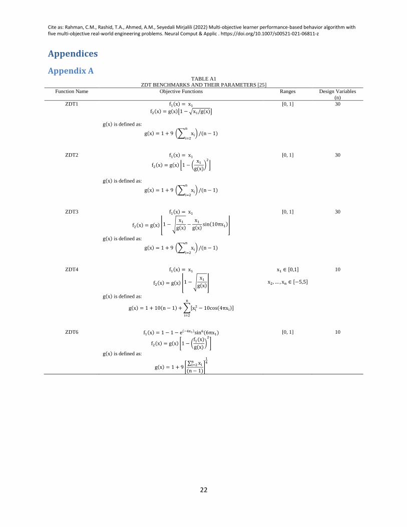
Cite as: Rahman, C.M., Rashid, T.A., Ahmed, A.M., Seyedali Mirjalili (2022) Multi-objective learner performance-based behavior algorithm with five multi-objective real-world engineering problems. Neural Comput & Applic . https://doi.org/10.1007/s00521-021-06811-z
22
Appendices
Appendix A TABLE A1
ZDT BENCHMARKS AND THEIR PARAMETERS [25]
Function Name Objective Functions Ranges Design Variables
(n)
ZDT1 f1(x) = x1
f2(x) = g(x)⌊1 − √x1/g(x)⌋
g(x) is defined as:
g(x) = 1 + 9 (∑ xi
n
i=2) /(n − 1)
[0, 1] 30
ZDT2 f1(x) = x1
f2(x) = g(x) ⌊1 − (x1
g(x))
2
⌋
g(x) is defined as:
g(x) = 1 + 9 (∑ xi
n
i=2) /(n − 1)
[0, 1] 30
ZDT3 f1(x) = x1
f2(x) = g(x) ⌊1 − √x1
g(x)−
x1
g(x)sin(10πx1)
⌋
g(x) is defined as:
g(x) = 1 + 9 (∑ xi
n
i=2) /(n − 1)
[0, 1] 30
ZDT4 f1(x) = x1
f2(x) = g(x) ⌊1 − √x1
g(x)
⌋
g(x) is defined as:
g(x) = 1 + 10(n − 1) + ∑[xi2 − 10cos(4πxi)]
n
i=2
x1 ∈ [0,1]
x2, … , xn ∈ [−5,5]
10
ZDT6 f1(x) = 1 − 1 − e(−4x1)sin6(6πx1)
f2(x) = g(x) [1 − (f1(x)
g(x))
2
]
g(x) is defined as:
g(x) = 1 + 9 [∑ xi
ni=2
(n − 1)]
14
[0, 1] 10