solving stochastic multi-objective programming in multi-attribute portfolio selection through the...

DIPARTIMENTO DI SCIENZE ECONOMICHE AZIENDALI E STATISTICHE

Via Conservatorio 7 20122 Milano

tel. ++39 02 503 21501 (21522) - fax ++39 02 503 21450 (21505) http://www.economia.unimi.it

E Mail: [email protected]

Lavoro presentato alla Conferenza internazionale MAF ’08, Venezia, 26-28 marzo 2008

SOLVING STOCHASTIC MULTI-OBJECTIVE PROGRAMMING THROUGH THE GP MODEL

BELAID AOUNI CINZIA C OLAPINTO DAVIDE LA TORRE

Working Paper n. 2008-18 GIUGNO 2008

Solving Stochastic Multi-ObjectiveProgramming through the GP model

Belaid Aouni, Cinzia Colapinto and Davide La Torre

Abstract The aim of this paper is to present an approach for solving the StochasticMulti-Objective Programming (SMOP) through the Goal Programming (GP) model.We introduce a deterministic equivalent formulation and we show how GP can pro-vide solutions to SMOP. The proposed method will be illustrated through a numer-ical example from the Tunisian stock exchange market.

1 Deterministic multi-objective programming and goalprogramming

Within the multi-criteria decision aid paradigm, several criteria, objectives or at-tributes are considered simultaneously. These dimensions are usually conflicting andthe decision-maker will look for the solution of the best compromise. The generalformulation of the multi-objective programming models can be formulated as fol-lows: Optimize [ f1(x), f2(x), . . . , fp(x)] under the condition that x ∈ D⊂ Rn; wherefi(x) represents the i-th objective function and D designates the set of feasible so-lutions. Let us define a vector function f (x) := [ f1(x), f2(x), . . . , fp(x)]; accordingto this, a classical multi-criteria decision problem can be formulated as (let assumethat all objectives have to be minimized)

minx∈D

f (x). (1)

Belaid AouniLaurentian University, Sudbury, ON, P3E 2C6 Canada e-mail: [email protected]

Cinzia ColapintoUniversity of Milan, Milan, 20122 Italy e-mail: [email protected]

Davide La TorreUniversity of Milan, Milan, 20122 Italy e-mail: [email protected]

1

2 Belaid Aouni, Cinzia Colapinto and Davide La Torre

As usual, we say that a point x ∈ D is a global Pareto solution iff

f (D)⊆ f (x)+(−Rp+\0)c. (2)

The goal programming (GP) model is a well-known aggregating procedure for solv-ing multi-objective programming decision aid processes. This takes into accountsimultaneously several objectives and measured through heterogeneous units andscales are conflicting. Thus the obtained solution through the GP model representsthe best compromise that can be made by the decision maker. The GP model is basedon a satisfying philosophy. The GP model is a distance function where the deviationbetween the achievement and aspiration levels are to be minimized. In fact, bothpositive and negative deviations are unwanted. The first formulation of a GP modelwas presented by Charnes et al. ([11]) and Charnes and Cooper ([12]) and then usedby Lee ([20]) and Lee and Clayton ([21]). GP model is widely applied in severalfields such as: accounting and financial aspect of stock management, marketing,quality control, human resources, production and operations management (see [7]and [24]). According to Aouni and Kettani ([5]) the GP is still alive and supportedby a well established network of researchers and practionners. The popularity of theGP is due to the fact that is a simple model and easy to understand and to apply.Moreover, the GP formulation can be solved through some powerful mathemati-cal programming software such as Lindo and CPLEX. The standard mathematicalformulation of the GP model (see [11]) is as follows:

minp

∑i=1

(δ+i +δ

−i ) (3)

subject tofi(x)+δ

−i −δ

+i = gi, (i = 1 . . . p) (4)

x ∈ D, δ+i ,δ−i ≥ 0, (i = 1 . . . p) (5)

where δ+i and δ

−i are, respectively, the positive and the negative deviations with

respect to the aspiration levels (goals) gi, i = 1, . . . , p.

2 Stochastic multi-objective programming

Stochastic multi-objective programming (SMOP) represents the natural extensionof deterministic multi-objective programming to stochastic contexts. In practicalapplications it is easy to find situations in which the Decision Maker (DM) wishesto optimize several objectives which depend on some random parameters. The factthat the objectives of the decision-making context depend on random parametersmakes the objectives random variables too; so a point in the domain could be anefficient solution of the problem only when some realizations of the random param-eters occur. For this reason, several definitions of efficiency have been introduced.

Solving SMOP through the GP model 3

The solution of such situations usually involves the transformation of the SMOPinto its deterministic equivalent (see [1],[9] and [26]). The aim of this paper is toshow how the GP model can be used for solving deterministic equivalent problemsassociated to SMOP.

Let consider (Ω ,F ,P) be a probability space and consider f : Rn×Ω → Rp befunction such that f (x, ·) is a random variable for each fixed x ∈ X (which means itis measurable for each fixed x) and f (·,ω) is continuous for a.e. ω ∈ Ω . We alsosuppose that for all x ∈ X the random variables f (x, ·) have finite first and secondorder moments, that is the following integrals are finite:

E( f (x, ·)) =∫

Ω

f (x,ω)dP(ω) = (E( f1(x, ·)), . . . ,E( fp(x, ·))) (6)

σ2( f (x, ·)) = E( f (x,ω)−E( f (x, ·)))2 (7)

for all x ∈ Rn. Let D : Ω ⇒ X be a compact random set, that is D(ω) ⊆ X is acompact set for a.e. ω ∈ Ω . A compact random set in Rn is a measurable mappingfrom (Ω ,F ,P) into the family H (Rn) of compact sets in Rn endowed with thetopology generated by the Hausdorff distance dH defined as

dH(A,B) = maxmaxx∈A

miny∈B

d(x,y),maxx∈B

miny∈A

d(x,y) (8)

and the corresponding Borel σ -algebra. Let us recall that for a given A∈H (Rn) thenorm of A is defined as ‖A‖= sup‖x‖ : x ∈ A. A random vector ξ is a selection ofa random set D if ξ (ω) ∈ D(ω) almost surely. Every non-empty random compactset D has at least one selection (see [17]). If at least one selection of D is integrablewe can define the Aumann expectation of D as the set of the expectations of all itsintegrable selections,

E(D) = E(ξ ) : ξ is an integrable selection ofD. (9)

The details of the Aumann expectation concepts can be found for instance in ([8]).As usual, we suppose that given a,b ∈ Rp, a ≥ b iff b−a ∈ Rp

+. Consider now thefollowing program (SMOP):

minx∈D(ω)

f (x,ω). (10)

Using the assumption we did before, we get that the SMOP has at least a solutionover D for a.e. ω ∈ Ω . These developments will be illustrated through examples 1and 2.

Example 1. Let us consider the minimization of following quadratic multi-objectivefunction [ f1, f2, f3] = [ξ11x2

1 +ξ12x22,ξ21x1 + x2,x1 +ξ22x2] subject to:


ξ11x1 +ξ12x2 ≤ 4x1,x2 ≤ 3x1,x2 ≥ 0x1,x2 ∈ N

(11)

As example, suppose that c = (ξ11,ξ12,ξ21,ξ22) is a random vector multinormalwith expected valued (0.5,1,1,2.5) and with positive definite covariance matrixdefined by:

25 0 0 30 25 3 00 3 1 03 0 0 9

(12)

Also in this case D(ω) is the feasible set which is defined through the above system.

Example 2. Let ξ : Ω→Rs be a random vector and consider the following quadraticstochastic multi-objective program (where, for simplicity, we write ξ (ω) = ξω ):

minZ = xA(ξω)x+b(ξω)x+ l(ξω) (13)

subject to:d11(ξω)x1 +d12(ξω)x2 + . . .+d1n(ξω)xn ≤ c1(ξω)

d21(ξω)x1 +d22(ξω)x2 + . . .+d2n(ξω)xn ≤ c2(ξω)

. . .

ds1(ξω)x1 +ds2(ξω)x2 + . . .+dsn(ξω)xn ≤ cs(ξω)

(14)

where A(ξω) = (A1(ξω),A2(ξω), . . . ,Ap(ξω)) ∈ Rn×n×p, b(ξω)=(b1(ξω),b2(ξω),. . . ,bp(ξω) ∈ Rn×p and l(ξω)=(l1(ξω), l2(ξω), . . . , lp(ξω)) ∈ Rp. We observe thatthe inequality constraints describe a random set D(ξω). One usually can find thiskind of decision-making situations in portfolio selection; where the objectives canbe the earn and the risk of the stock set, D(ξ ) represents technological coefficientsand c(ξ ) denote random variables which describe resource limitations.

The following result states a strong law of large numbers for Minkowski sumsand is due to Vitale [28].

Theorem 1. [28] Let A1, A2, . . . be a sequence of independent, identically dis-tributed (iid) random sets with E(‖A‖) < ∞. Then

A1 +A2 + . . .An

n→ E(A) (15)

a.s. as n → ∞ with respect to the Hausdorff distance dH and the sum is theMinkowski sum between sets.


3 Deterministic equivalent formulations and GP model

Following Caballero et al ([9]), we can introduce the following deterministic multi-objective equivalent programs associated to SMOP. Let D be the expectation of therandom set D(ω), that is D = E(D(·)). Notice that in [9] the authors do not assumeany randomness on the set of constraints so these definitions are an extension ofthem.

Definition 1. A point x ∈ D is expected-value Pareto optimal solution of the SMOPif it is a Pareto optimal solution of the following problem

minx∈D

E( f (x, ·)) := (E( f1(x, ·)), . . . ,E( fp(x, ·))) (16)

where E( fi(x, ·)) is the expectation value of the random variable fi(x, ·) for eachfixed x ∈ D.

Definition 2. A point x ∈ D is minimum-variance Pareto optimal solution of theSMOP problem if it is a Pareto optimal solution of the following problem

minx∈D

σ2( f (x, ·)) :=

(σ

2( f1(x, ·)), . . . ,σ2( fp(x, ·)))

(17)

where σ2( fi(x, ·)) is the variance of the random variable fi(x, ·) for each fixed x∈ D.

Definition 3. A point x∈ D is an expected-valued standard deviation Pareto optimalsolution of the SMOP problem if it is a Pareto optimal solution of the followingprogram

minx∈D

(E( f (x, ·),σ( f (x, ·)) := (E( f1(x, ·)), . . . ,E( fp(x, ·),σ( f1(x, ·), . . . ,σ( fp(x, ·))(18)

where σ( f (x, ·)) is the standard deviation of the random variable f (x, ·) for eachfixed ω ∈Ω .

Consider now the aspiration levels gi (i = 1 . . . p) and suppose they are randomvariables gi : Ω → R with finite first and second order moments. Let E(gi) andσ2(gi) be the expectation values and the variances of gi, respectively. Consider thefollowing goal programming model associated to problems (16), (17) and (18), re-spectively.

GP Model 1:

minp

∑i=1

(δ+i +δ

−i ) (19)

subject to:


E( fi(x, ·))+δ−i −δ

+i = E(gi) i = 1 . . . p

x ∈ D

δ+i ,δ−i ≥ 0 i = 1 . . . p

GP Model 2:

minp

∑i=1

(δ+i +δ

−i ) (20)

subject to:σ2( fi(x, ·))+δ

−i −δ

+i = σ2(gi), i = 1 . . . p

x ∈ D, δ+i ,δ−i ≥ 0

GP Model 3:

minp

∑i=1

(δ+i +δ

−i +ϑ

+i +ϑ

−i ) (21)

subject to:E( fi(x, ·))+δ

−i −δ

+i = E(gi), i = 1 . . . p

σ( fi(x, ·))+ϑ−i −ϑ

+i = σ(gi), i = 1 . . . p

x ∈ D, δ+i ,δ−i ,ϑ+,ϑ−i ≥ 0 i = 1 . . . p

Suppose we take a sample of observations of the random vector f (x,ω) and of therandom set D(ω), say ( f (x,ω1), f (x,ω2), . . . f (x,ωm)) ∈ Rp×m and (D(ω1),D(ω2). . .D(ωm)) ∈ (H (Rn))m. If the observations are independent and identically dis-tributed (i.i.d.) we can get an estimation of the mean and the variance of E( f (x, ·)),σ2( f (x, ·)) and E(D(·)) using the formulas

E( f (x, ·))≈ ∑mk=1 f (x,ωk)

m

σ2( f (x, ·))≈ ∑mk=1( f (x,ωk)−E( f (x,·)))2

m−1

E(D(·))≈ ∑mk=1 D(ωk)

m

where the last sum is the Minkowki sum between sets.

4 Numerical example

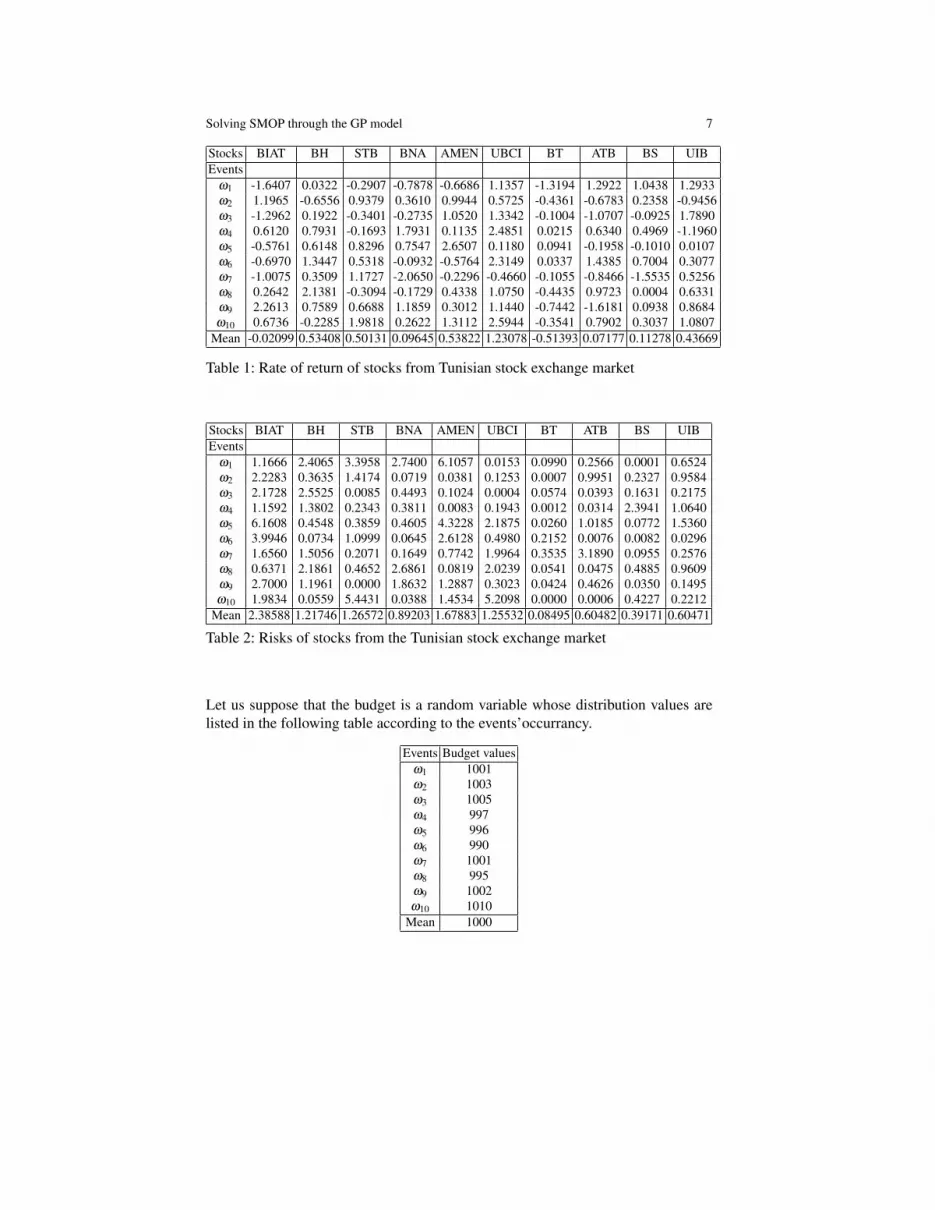
Let us consider the following data which have been simulated starting from real dataabout ten stocks of the Tunisian stock exchange available in [1]. Table 1 describesthe return rate while Table 2 represents the level of risk. The stocks are supposed tobe independent.


Stocks BIAT BH STB BNA AMEN UBCI BT ATB BS UIBEvents

ω1 -1.6407 0.0322 -0.2907 -0.7878 -0.6686 1.1357 -1.3194 1.2922 1.0438 1.2933ω2 1.1965 -0.6556 0.9379 0.3610 0.9944 0.5725 -0.4361 -0.6783 0.2358 -0.9456ω3 -1.2962 0.1922 -0.3401 -0.2735 1.0520 1.3342 -0.1004 -1.0707 -0.0925 1.7890ω4 0.6120 0.7931 -0.1693 1.7931 0.1135 2.4851 0.0215 0.6340 0.4969 -1.1960ω5 -0.5761 0.6148 0.8296 0.7547 2.6507 0.1180 0.0941 -0.1958 -0.1010 0.0107ω6 -0.6970 1.3447 0.5318 -0.0932 -0.5764 2.3149 0.0337 1.4385 0.7004 0.3077ω7 -1.0075 0.3509 1.1727 -2.0650 -0.2296 -0.4660 -0.1055 -0.8466 -1.5535 0.5256ω8 0.2642 2.1381 -0.3094 -0.1729 0.4338 1.0750 -0.4435 0.9723 0.0004 0.6331ω9 2.2613 0.7589 0.6688 1.1859 0.3012 1.1440 -0.7442 -1.6181 0.0938 0.8684ω10 0.6736 -0.2285 1.9818 0.2622 1.3112 2.5944 -0.3541 0.7902 0.3037 1.0807

Mean -0.02099 0.53408 0.50131 0.09645 0.53822 1.23078 -0.51393 0.07177 0.11278 0.43669

Table 1: Rate of return of stocks from Tunisian stock exchange market

Stocks BIAT BH STB BNA AMEN UBCI BT ATB BS UIBEvents

ω1 1.1666 2.4065 3.3958 2.7400 6.1057 0.0153 0.0990 0.2566 0.0001 0.6524ω2 2.2283 0.3635 1.4174 0.0719 0.0381 0.1253 0.0007 0.9951 0.2327 0.9584ω3 2.1728 2.5525 0.0085 0.4493 0.1024 0.0004 0.0574 0.0393 0.1631 0.2175ω4 1.1592 1.3802 0.2343 0.3811 0.0083 0.1943 0.0012 0.0314 2.3941 1.0640ω5 6.1608 0.4548 0.3859 0.4605 4.3228 2.1875 0.0260 1.0185 0.0772 1.5360ω6 3.9946 0.0734 1.0999 0.0645 2.6128 0.4980 0.2152 0.0076 0.0082 0.0296ω7 1.6560 1.5056 0.2071 0.1649 0.7742 1.9964 0.3535 3.1890 0.0955 0.2576ω8 0.6371 2.1861 0.4652 2.6861 0.0819 2.0239 0.0541 0.0475 0.4885 0.9609ω9 2.7000 1.1961 0.0000 1.8632 1.2887 0.3023 0.0424 0.4626 0.0350 0.1495ω10 1.9834 0.0559 5.4431 0.0388 1.4534 5.2098 0.0000 0.0006 0.4227 0.2212

Mean 2.38588 1.21746 1.26572 0.89203 1.67883 1.25532 0.08495 0.60482 0.39171 0.60471

Table 2: Risks of stocks from the Tunisian stock exchange market

Let us suppose that the budget is a random variable whose distribution values arelisted in the following table according to the events’occurrancy.

Events Budget valuesω1 1001ω2 1003ω3 1005ω4 997ω5 996ω6 990ω7 1001ω8 995ω9 1002ω10 1010

Mean 1000


On the other hand, let us suppose for many reasons that the following constraintshave to be satisfied:

BIAT +BH ≤ 200UBCI ≤ 100AMEN ≥ 50

What we show in this example is how to get the expected-value Pareto solution ofthe portfolio selection under study. On the other hand, one could consider the otherdefinitions of Pareto solutions we introduced in the previous section. The mathe-matical formulation based on this data can be as follows:

maxZ1 =−0.02099∗BIAT +0.53408∗BH +0.50131∗ST B+0.09645∗BNA+0.53822∗AMEN +1.23078∗UBCI−0.51393∗BT +0.07177∗AT B+0.11278∗BS +0.43669∗UIB

(22)minZ2 = 2.38588∗BIAT +1.21746∗BH +1.26572∗ST B+0.89203∗BNA+1.67883∗AMEN +1.25532∗UBCI +0.08495∗BT +0.60482∗AT B+0.39171∗BS +0.60471∗UIB

(23)subject to:

BIAT +BH +ST B+BNA+AMEN +UBCI +BT +AT B+BS +UIB = 1000BIAT +BH ≤ 200UBCI ≤ 100AMEN ≥ 50BIAT,BH,ST B,BNA,AMEN,UBCI,BT,AT B,BS,UIB≥ 0

(24)Let g1 and g2 be the two random aspiration levels for the objective functions Z1 andZ2 whose values are listed in the following table.

Events g1 g2ω1 1250.61 0.01ω2 1230.15 0.04ω3 1220.11 0.02ω4 1210.55 0.10ω5 1200.43 0.02ω6 1232.13 0.01ω7 1220.15 0.04ω8 1217.83 0.06ω9 1240.74 0.20ω10 1285.1 0.20

Mean 1230.780 0.07

Let us consider the following GP model:

minZ = δ+1 +δ

−1 +δ

+2 +δ

−2 (25)

subject to:


−0.02099∗BIAT +0.53408∗BH +0.50131∗ST B+0.09645∗BNA+0.53822∗AMEN +1.23078∗UBCI−0.51393∗BT +0.07177∗AT B+0.11278∗BS +0.43669∗UIB−δ

+1 +δ

−1 = 1230.780

2.38588∗BIAT +1.21746∗BH +1.26572∗ST B+0.89203∗BNA+1.67883∗AMEN +1.25532∗UBCI +0.08495∗BT +0.60482∗AT B+0.39171∗BS +0.60471∗UIB−δ

+2 +δ

−2 = 0.07

BIAT +BH +ST B+BNA+AMEN +UBCI +BT +AT B+BS +UIB = 1000BIAT +BH ≤ 200UBCI ≤ 100AMEN ≥ 50BIAT,BH,ST B,BNA,AMEN,UBCI,BT,AT B,BS,UIB≥ 0δ

+1 ,δ−1 ,δ+

2 ,δ−2 ≥ 0

The solution of this program is BIAT = BH = ST B = BNA = BT = AT B = BS = 0,AMEN = 50, UBCI = 100, UIB = 850.

5 Conclusion

In this paper we have considered deterministic equivalent formulation of StochasticMulti-objective Optimization Programs and formulated a GP model that allows toobtain the best solutions to these decision-making situations. The SMOP we con-sider involves a random feasible set. The notion of deterministic equivalent formu-lation we introduce generalizes the one introduced by Caballero et al in [9] sincein order to get it we consider the expectations of random sets according to the def-inition in [28]. The developed model has been illustrated by an example from theTunisian stock exchange market.

Acknowledgements

This work has been carried out during research periods of Cinzia Colapinto andDavide La Torre at School of Commerce and Administration of the Laurentian Uni-versity, Sudbury, Ontario, Canada. We thank Prof. Belaid Aouni for this opportunity.

References

1. Abdelaziz F.B., Aouni B., El Fayedh R., Multi-objective stochastic programming for port-folio selection, European J.Oper.Res., 177 (2007), 1811-1823.


2. Abdelaziz F.B., Lang P., Nadeau R., Dominance and efficiency in multicriteria decisionunder uncertainty, Theory and decisions, 47, 3 (1999), 191-211.

3. Abdelaziz F.B., Lang P., Nadeau R., Distributional unanimity multiobjective stochastic lin-ear programming, in Multicriteria analysis: Proceedings of the XIth International Confer-ence on MCDM (Climaco, J. Ed.), Springer-Verlag, Berlin, 225-236..

4. Aouni B., Linearisation des expressions quadratiques en programmation mathematique: desbornes plus efficaces. Administrative Sciences Association of Canada, Management Sci-ence, 17 (1996), 38-46.

5. Aouni B., Kettani O., Goal programming model: a glorious history and a promising future,European J.Oper.Res., 133, 2 (2001), 1-7.

6. Aouni B., Kettani O., Martel J-M., Estimation through imprecise goal programming model,in Advances in multi-objective and goal programming, Lecture Notes in Economics andMathematical Systems, vol. 455 (1997), Springer, 120-130.

7. Aouni B., Abdelaziz F.B., Martel J-M., Decision-maker’s preferences modeling in thestochastic goal programming, European J.Oper.Res., 162 (2005), 610-618.

8. Aumann R.J., Integrals of set-valued functions, J. Math. Anal. Appl. 12 (1965), pp. 112.9. Caballero R., Cerda E., Munoz M.M., Rey L., Stancu-Minasian I.M., Efficient solution

concepts and their relations in stochastic multiobjective programming, J.Opt.Th.App., 110,1 (2001), 53-74.

10. Caballero R., Cerda E., Munoz M.M., Rey L., Stochastic approach versus multiobjectiveapproach for obtaining efficient solutions in stochastic multiobjective programming prob-lems, European J.Oper.Res., 158 (2004), 633-648.

11. Charnes A., Cooper W.W., Chance constraints and normal deviates,J.Amer.Stat.Association, 57 (1952), 134-148.

12. Charnes A., Cooper W.W., Chance-constrained programming, Management Science, 6(1959), 73-80.

13. Charnes A., Cooper W.W., Management models and industrial applications of linear pro-gramming, Wiley, 1961.

14. Charnes A., Cooper W.W., Deterministic equivalents for optimising and satisfying underchance constraints, Operations Research, 11 (1968), 11-39.

15. Charnes A., Cooper W.W., Ferguson R., Optimal estimation of executive compensation bylinear programming, Management Science, 1 (1955), 138-351.

16. Contini B., A stochastic approach to goal programming, Oper.Res., 16, 3 (1968), 576-586.17. Fernandeza I.C., Molchanovb I., A stochastic order for random vectors and random sets

based on the Aumann expectation, Stat. Prob. Letters, 63 (2003) 295-305.18. Goicoechea A., Hansen D.R., Duckstein L., Multiobjective decision analysis with engineer-

ing and business applications, Wiley, New York, 1982.19. Kharrat A., Chabchoub H., Aouni B., Smaoui S., Serial correlation estimation through the

imprecise goal programming model, European J.Oper.Res., 177 (2007), 1839-1851.20. Lee S.M., Goal programming for decision analysis of multiple objectives, Sloan Manage-

ment Review, 14 (1973), 11-24.21. Lee S.M., Clayton S.R., A goal programming model for academic resource allocation, Man-

agement Science, 18, 8 (1972), B395-B408.22. Lee S.M., Olson D.L., Gradiend algorithm for chance-constrained nonlinear goal program-

ming, European J.Oper.Res., 22, 3 (1985), 359-369.23. Martel J-M., Aouni B., Diverse imprecise goal programming model formulations, J.Global

Opt., 12 (1998), 127-138.24. Romero C., Handbook of critical issues in goal programming, Pergamon Press, 1991.25. Sawaragi Y., Nakayama H., Tanino T., Theory of multiobjective optimization, Academic

Press, New York, 1985.26. Stancu-Minasian I.M., Stochastic programming with Multiple Objective Functions, D. Rei-

del Publishing Company, Dordrecht, 1984.27. Stancu-Minasian I.M., Tigan S., The vectorial minimum risk problem, in Proceedings of

the Colloquium on Approximation and Optimization, Cluj-Napoca, 1984, 321-328.


28. Vitale R.V., An alternate formulation of mean value for random geometric figures. Journalof Microscopy, 151, 3, 1988, 197204.

29. White D.J., Optimality and efficiency, Wiley, Chichester, 1982.

solving stochastic multi-objective programming in multi-attribute portfolio selection through the...

Documents