adaptive anisotropic meshing for steady convection-dominated problems

Adaptive Anisotropic Meshes for Steady-StateConvection-Dominated Problems

Hoa Nguyen

School of Computational Science& Department of Mathematics

Florida State [email protected]

Collaborators: John Burkardt, Max Gunzburger, Lili Ju

Adaptive Anisotropic Meshes

Model Equation

Let Ω ⊂ R2 be a bounded polygonal domain with Lipschitz boundary ∂Ω.Consider the stationary model of the convection diffusion equation:

−a4u + v · ∇u = f in Ωu = g on ∂Ω

(1)

where

• a > 0 is a constant diffusion term;

• v(x) ∈ W 1,∞(Ω) is a convective field;

• f(x) ∈ L2(Ω) is an outer source function;

• g ∈ H12(∂Ω) is the Dirichlet boundary condition.

Adaptive Anisotropic Meshes 1

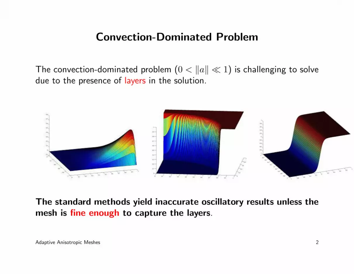
Convection-Dominated Problem

The convection-dominated problem (0 < ‖a‖ 1) is challenging to solvedue to the presence of layers in the solution.

The standard methods yield inaccurate oscillatory results unless themesh is fine enough to capture the layers.


Existing Methods

• Stabilized schemes: the upwind techniques ([1]), the Galerkin/ least-squares method ([2]) and the streamline upwind Petrov Galerkin method(SUPG) ([3]) (mostly done on uniform meshes).

• A posteriori error estimator: detects layer regions for mesh refinement([4]). The refined meshes can be isotropic (regular elements) oranisotropic (stretched elements).

Many researchers have worked on this convection-dominatedproblem since the mid 1980s, but no satisfactory method hasbeen found to completely eliminate the non-physical oscillations inthe solutions.


Our Motivation

To resolve this problem, we realize:

• A good choice of stabilized method can lead to both small discretizationerrors and rapid convergence.

• An optimized meshing scheme can reduce the computational cost andimprove the accuracy of the solution. It is desirable to use anisotropicmeshes, which distribute more points in the layer regions such that themesh elements are stretched along the layers.

• The stabilized method and the optimized meshing scheme can be tiedtogether by a metric tensor, which is computed from the approximatesolution of the stabilized method and then used to generate the mesh.


The Ingredients for Our Algorithm

• A good stabilized method.

• An reliable metric tensor.

• An optimized meshing scheme.


1st Ingredient: the Stabilized Method

The streamline upwind Petrov Galerkin method (SUPG): extradiffusion is added in the streamline direction v · ∇u.

Set H1D(Ω) = φ ∈ H1(Ω) : φ = g on ∂Ω. Assume that τ is a

triangulation of Ω, and VD,h ⊂ H1D(Ω) be the space of continuous,

piecewise linear functions over τ which satisfy the Dirichlet boundarycondition on ∂Ω.

Then the SUPG variational formulation of problem (1) is:

Find uh ∈ VD,h:Bδ(uh, vh) = 〈Fδ, vh〉, ∀vh ∈ VD,h

Bδ(uh, vh) = a(∇uh,∇vh) + (v · ∇uh, vh)+ΣT∈τδT (−a4uh + v · ∇uh, v · ∇vh)T

〈Fδ, vh〉 = (f, vh) + ΣT∈τδT (f, v · ∇vh)T


The Stabilization Parameter δT

The discrete solution uh exists and is unique if the stabilization parametersδT are sufficiently small for each element T . We choose

δT =hmin,T

2‖v‖L2(T )

where hmin,T is the average length of the edges projected onto theconvective field v(x).


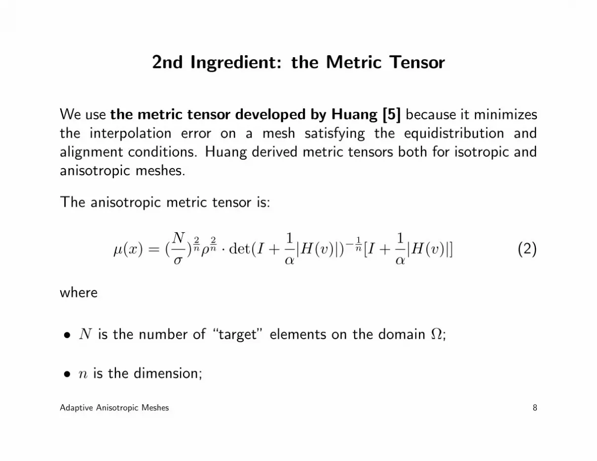
2nd Ingredient: the Metric Tensor

We use the metric tensor developed by Huang [5] because it minimizesthe interpolation error on a mesh satisfying the equidistribution andalignment conditions. Huang derived metric tensors both for isotropic andanisotropic meshes.

The anisotropic metric tensor is:

µ(x) = (N

σ)

2nρ

2n · det(I +

1α|H(v)|)−1

n[I +1α|H(v)|] (2)

where

• N is the number of “target” elements on the domain Ω;

• n is the dimension;


• α is the intensity parameter defined implicitly through the equation:∫Ω

ρ(x) dx = |Ω|1−β ;

• ρ = ‖I + 1α|H(v)|‖

mnq2(n+(2−m)q) det(I + 1

α|H(v)|)(2−m)q

2(n+(2−m)q) is theadaptation function;

• β indicates roughly the percentage of the mesh points concentrated inthe regions of large ρ;

• Wm,q is the interpolation error norm (L2-norm: m = 0, q = 2, H1-norm: m = 1, q = 2);

• H(v) is the Hessian matrix of v.


The Meaning of the Metric Tensor

A metric tensor ↔ A positive definite matrix ↔ An ellipse

Let P be a point in Ω, a metric tensor at P : M(P ) = ETUE

E =

(cosθ sinθ

−sinθ cosθ

)U =

(λ1(P ) 0

0 λ2(P )

)

The unitary volume condition:∫

T

√det(M(x))dx = 1,∀T ∈ T .


3rd Ingredient: the Optimized Meshing Scheme

The optimized meshing scheme contains two parts.

• Part 1: create a mesh directly from the metric tensor without anyinternal optimization. Simmetrix [6] is a commercially available softwarepackage which meets this requirement.

• Part 2: optimize the mesh such that mesh elements are stretched alongthe layers and errors are distributed uniformly. Given a metric tensor,Anisotropic Centroidal Voronoi Tessellations (ACVT) [7] distributes thenodes of mesh elements by minimizing a cost function to improvethe element quality and reduce the sizing distortion. Consequently,the nodes become the centers of mass (centroids) of the associatedVoronoi regions with respect to the given metric tensor.


Anisotropic Centroidal Voronoi Tessellations (ACVT)For simplicity, assume the metric tensor is a 2× 2 identity matrix.

Left: the generators (the blue dots) do not coincide with the centers of mass (the red dots).

Right: the dots are simultaneously the generators and the centers of mass.

The process of moving the initial nodes to the optimal positions (centersof mass) is done by the generalized Lloyd iteration method.


The Generalized Lloyd Iteration Method

⇒oneiteration

⇒manyiterations

A step of Lloyd’s method (top) and the ACVT mesh (bottom) with respect to an identity metric tensor.


The Dual Triangulation Mesh of ACVT Mesh

After projecting the outer points of the ACVT mesh onto the associatedboundary, the dual triangulation mesh is constructed:

The ACVT mesh (blue grid) and the dual triangulation mesh (green grid) with respect to an identity metric tensor.


The Proposed Algorithm

Let Ω ⊂ R2 be a bounded polygonal domain with Lipschitz boundary ∂Ω.

Given an initial coarse mesh, approximate the solution of equation (1) bythe SUPG to compute the metric tensor.

For each level of the refinement, the following steps are done:

• Step 1: generate ACVT mesh based on the computed metric tensor.

• Step 2: solve the equation (1) on the optimized mesh of step 1.

• Step 3: use the approximate solution from step 2 to compute themetric tensor.


Numerical Experiment

We consider the convection dominated equation (1) on Ω = [0, 1]2.

Let a = 10−8, v = (1, 0) and assume the Dirichlet condition on thedomain boundary ∂Ω.

The right-hand side f and the boundary condition are chosen such thatthe solution is:

u(x, y) =

(4x− 1)(3− 4x) for (x, y) ∈ [0.25, 0.75]2,0 otherwise


Exact SolutionThis solution is challenging to solve because it is discontinuous andpossesses two interior layers at x ∈ (0.25, 0.75), y = 0.25 and x ∈(0.25, 0.75), y = 0.75.

This example is similar to the one described in [8] where the existingmethods fail to resolve the nonphysical oscillations near the layers of thesolution.


Adaptive Meshes

Let nt be the number of triangles in a mesh. Our algorithm adaptivelygenerates isotropic and anisotropic meshes to solve the equation (1).

Figure 1 Left: Isotropic mesh (nt = 7498). Right: Anisotropic mesh (nt = 7344).


Approximate Solutions

Figure 2 Approximate solutions on isotropic meshes.

Left: Galerkin, nt = 321, L2 error = 10.17. Right: SUPG, nt = 14308, L2 error = 0.016.

Figure 3 Approximate solutions on anisotropic meshes.

Left: Galerkin, nt = 228, L2 error = 2.535. Right: SUPG, nt = 7344, L2 error = 0.009.


Discussion

The solution (figure 3, right) discretized by the SUPG and solved on ouradaptive anisotropic meshes achieves the best accuracy and convergencerate compared with the others.

These results agree with the theory of the three ingredients in ouralgorithm:

• the SUPG method is essential to resolve the non-physical oscillationsin this type of solution;

• the numerical approximation has better convergence rate on ouradaptive anisotropic meshes than on isotropic or uniform ones;

• our algorithm significantly reduces the computational cost for solvingthis equation.


Conclusion

Compared with the existing methods, our algorithm has substantiallyimproved the numerical approximation for the steady-state convectiondiffusion equation when convection dominates diffusion.

The results converges at a quasi-optimal rate and with low computationalcost.

We will extend our research to the time-dependent case and continueoptimizing our schemes and algorithms to obtain the best numericalapproximation.

Thank You!


References

[1] I. J. C. Heinrich, P.S. Huyakorn, O. C. Zienkiewicz andA. R. Mitchell; An “upwind” finite element scheme for two-dimensional convective transport equation, Int. J. Numer. MethodsEngrg. 11 1977 pp 131–143.

[2] T. J. R. Hughes, L. P. Franca and G. M. Hulbert; A newfinite element formulation for computational fluid dynamics. VIII.The Galerkin/least-squares method for advective-diffusive equations,Computer Methods in Applied Mechanics and Engineering 73 1989pp 173–189.

[3] A. N. Brooks , T. J. R. Hughes; Streamline upwind/Petrov-Galerkin formulations for convection dominated flows with particularemphasis on the incompressible Navier-Stokes equations, ComputerMethods in Applied Mechanics and Engineering 32 1982 pp 199–259.


[4] V. John; A numerical study of a posteriori error estimatorsfor convection-diffusion equations, Computer Methods in AppliedMechanics and Engineering 190 2000 pp 757–781.

[5] W. Huang; Metric tensors for anisotropic mesh generation, J.Comput. Phys. 204 2005 pp 633–665.

[6] Simmetrix software: http://www.simmetrix.com

[7] Q. Du, D. Wang; Anisotropic Centroidal Voronoi Tessellations andtheir Applications, SIAM. Journal on Scientific Computing 26 (3)2005 pp 737–761.

[8] V. John and P. Knobloch; A computational comparison ofmethods diminishing spurious oscillations in finite element solutionsof convection–diffusion equations, Proceedings of the ConferencePrograms and Algorithms of Numerical Mathematics 13 Prague,May 2831, 2006 (to appear).


adaptive anisotropic meshing for steady convection-dominated problems

Documents