numerical multiscale methods for a reaction dominated model
TRANSCRIPT
Comput. Methods Appl. Mech. Engrg. 201–204 (2012) 228–244
Contents lists available at SciVerse ScienceDirect
Comput. Methods Appl. Mech. Engrg.
journal homepage: www.elsevier .com/locate /cma
Numerical multiscale methods for a reaction-dominated model
Honório Fernando 1, Christopher Harder 1, Diego Paredes 2, Frédéric Valentin ⇑,1
Departamento de Matemática Aplicada, Laboratório Nacional de Computação Científica, Av. Getúlio Vargas, 333, 25651-070 Petrópolis, RJ, Brazil
a r t i c l e i n f o
Article history:Received 16 November 2010Received in revised form 25 May 2011Accepted 13 September 2011Available online 22 September 2011
Keywords:MultiscaleReaction–diffusion equationFinite element methodEnriched space
0045-7825/$ - see front matter � 2011 Elsevier B.V. Adoi:10.1016/j.cma.2011.09.007
⇑ Corresponding author. Tel.: +55 24 22336082; faxE-mail addresses: [email protected] (H. Fernando)
[email protected] (D. Paredes), [email protected] (F. Va1 The author is supported by CNPq/Brazil.2 The author is supported by CONICYT/Chile.
a b s t r a c t
A Galerkin enriched finite element method (GEM) is proposed for the singularly perturbed reaction–dif-fusion equation. This new method is an improvement on the Petrov–Galerkin enriched method (PGEM),where now the standard piecewise (bi)linear test space incorporates fine scales. This appears as the fun-damental ingredient for suppressing oscillations in the numerical solutions. Also, new parameter-freestabilized finite element methods derived from both the GEM and the PGEM are driven by local general-ized eigenvalue problems. In the process, jump stabilizing terms belonging to the class of CIP methodsemerge as a result of the enriching procedure. Interestingly, numerical results indicate that jump-basedstabilizations are unnecessary and sometimes undesirable when treating reaction-dominated problems.Finally, we establish relationships with more standard enriched and stabilized methods and show thatthe proposed methods outperform them numerically.
� 2011 Elsevier B.V. All rights reserved.
1. Introduction
Arising from realistic modeling in diverse fields such as biology(ecosystem or neuroscience models), chemistry (reactive pro-cesses), or in mechanical engineering (transport in porous media,turbulence model or wildfire problems, just to cite a few) is thereaction-dominated reaction–diffusion equation. Solutions to suchproblems exhibit boundary layers which must be handled carefullyby numerical schemes. Without such care, approximation of thegradient of the true solution in the natural norm is adversely af-fected, leading to non-physical oscillations in the numerical solu-tion. For example, solving this singularly perturbed model usingthe Galerkin method based on local polynomial interpolation re-quires specially refined meshes (Shishkin meshes [1], for instance)in regions containing boundary layers in order to avoid non-phys-ical oscillations. However, such an approach becomes increasinglyprohibitive for real-life problems defined on complex geometriesand demands prior knowledge of the position of sharp layers. Inthis work, we pursue the idea of constructing robust finite elementmethods for solving reaction-dominated problems on coarse(un)structured meshes.
Among the alternatives is the stabilized finite element method[2]. When applied to the reactive–diffusive model, numerical solu-tions can fulfill the maximum principle property on coarse meshes.The general idea is to select appropriate weak stabilizing terms to
ll rights reserved.
: +55 24 22336124., [email protected] (C. Harder),lentin).
be included in the Galerkin formulation. Several possibilities thatmodify the original formulation exist, among which are the addi-tion of weak terms depending on the gradient of the residual ofthe Lagrange equation [3–5] or the subtraction of weak termsdependent on the residual of the strong model [6,7] (see [8] for acomparison of the performance between several stabilizedmethods). In an attempt to build operator-independent stabilizedmethods, edge-based jump terms have been used to penalizeinter-element fluxes [9–11]. These stabilization alternatives arebalanced by parameters which must be carefully tuned in advance,as their values have a great impact on the accuracy of solutions.
The relationship of these stabilized methods with the Varia-tional Multiscale approach (VMS) [12] has been investigated tobetter understand the mechanism governing the design of the sta-bilization parameters. The Residual-Free Bubble (RFB) method[13,14] and the Petrov–Galerkin enriched (PGEM) methods[15,16] are examples of such an approach (see [17] for an over-view), wherein the standard polynomial space is enriched withfunctions which capture subgrid behavior. Such enrichment func-tions are computed from local boundary value problems arisingfrom a static condensation procedure. Thereby, the unsolved finescales are represented in terms of coarse ones through element-wise residuals. Furthermore, edge residuals play an important rolein the construction of enriching basis functions for the reaction–diffusion model [15]. This is, actually, the PGEM’s distinguishingfeature (see [18] for an overview) and allows the method to pro-duce solutions which are accurate in natural norms. Other ap-proaches rely on nonstandard polynomial basis functions, such asthe PUM (Partition of Unity Method). See [19] for a recentoverview.
H. Fernando et al. / Comput. Methods Appl. Mech. Engrg. 201–204 (2012) 228–244 229
This work presents a threefold contribution. First, a new Galer-kin enriched finite element method (GEM) is proposed by modify-ing the PGEM so that the test space is now defined so as to includefine scales. Such a feature was, indeed, restricted to the trial spacein [15]. Readers are invited to consider [20,21], where such a strat-egy was introduced by observing the presence of fine scales in thetest space in 1D leads to nodal exactness (analogous to what occursin the oscillatory elliptic case [22]). Numerical results show thatthe new method outperforms the original PGEM when the reaction(balanced by the element diameter) and diffusion coefficients arecomparable. This drawback for the PGEM, first pointed out numer-ically in [23], is the result of a resonance error analogous to whatoccurs with oscillatory coefficient models [24], and is explainedby the lack of convergence with respect to the gradient of the solu-tions for intermediate values of diffusive coefficient.
Second, the relationship between some well-establishednumerical strategies and the construction of enriching basis func-tions is considered. Namely, we draw comparisons with theedge-based Continuous Interior Penalty method (CIP) [10] andthe multiscale finite element method (MsFEM) [24]. As for the for-mer, the approach leads to a perturbation of the GEM with bound-ary terms that explicitly control the jump of the flux in a formequivalent to that of CIP methods.
To the best of the authors’ knowledge, this is the first time edge-based finite element methods for the reactive–diffusive equationare derived inside an enriching space strategy (see [25] and [26]for a related idea applied to the Darcy and Stokes models, respec-tively). The upshot of the approach is that no stabilization param-eter needs to be fixed. Also, we show that the most suitable MsFEMversion in [24] may be recovered from the present enhancing ideawith a modified right hand side. Numerical tests attest that thisdifference is fundamental to greatly reduce resonance errors.
Finally, stabilized finite element methods derived from the GEMand the PGEM [15] are introduced. These new methods are of theunusual finite element type [6], in which the elemental stabiliza-tion parameters are fixed through the action of the multiscale basisfunctions. This is a well-known strategy in the context of bubblefunction enrichment for advective–diffusive problems [27,28]. Fol-lowing the methodology [29] of producing stabilization parame-ters through enrichment functions, this idea is extended toreaction-dominated problems using local generalized eigenvalueproblems. The GEM and its stabilized method counterpart arenumerically compared with more classical stabilized methods inorder to highlight the influence of the extra term on the numericalsolution’s accuracy. In particular, it appears that CIP-like stabiliza-tion terms are unable to provide adequate stabilization in reaction-dominated regimes and the MsFEM overpredicts the exactsolution.
The outline of this paper is as follows: notation and definitionsclose out the current section. Next, the model and some prelimin-ary results are given in Section 2. The enriching space methodologyis presented and used to obtain the GEM in Section 3. Sections 4and 5 are dedicated to establishing a relationship of the enrichingspace approach with the MsFEM and CIP methods, respectively.Section 6 is devoted to stabilized methods related to the GEM. Fi-nally, numerical tests are found in Section 7, followed by conclu-sions in Section 8.
1.1. Notation and preliminaries
This section introduces definitions and notation used through-out. Let D be a bounded set in Rd, d 2 {1,2} and suppose L2(D) isthe usual space of square integrable functions over D. This spaceis equipped with an inner-product (�, �)D. The space Hl(D) is thesubspace of L2(D) whose functions have square integrable deriva-tives up to order l. The H1(D) semi-norm is defined by j � j1,D.
Furthermore, the subspace H10ðDÞ � H1ðDÞ consists of functions
with support in D, H�1(D) stands for the dual space of H10ðDÞ, and
the mean value of function v 2 L2(D) is denoted by PDðvÞ :¼ 1jDjR
D v .In what follows, X denotes an open bounded domain in R2 with
polygonal boundary @X, and x = (x,y) is a typical point in X. LetfT hg be a family of regular partitions of X consisting of triangles(or rectangles) K with boundary @K composed of edges F. The setof internal edges of the partition T h is denoted by Eh. Diametersof K and F are denoted by hK and hF, respectively, andh :¼maxfhK : K 2 T hg > 0. The mesh regularity condition impliesthere exists a positive constant C such that hF 6 hK 6 ChF, for allF # @K. Also, a unit normal vector nF is fixed, once and for all, foreach F ¼ K \ K 0 2 Eh, where K; K 0 2 T h, with the only restrictionbeing that it coincides with the unit outward normal vector whenF # @X. Moreover, given F 2 Eh and a function q, one denotes bysqt its jump, defined by:
sqtðxÞ :¼ limd!0þ
qðxþ dnFÞ � limd!0�
qðxþ dnFÞ ð1Þ
and sqt = 0 if F # @X.The classic space of bubble functions H1
0ðT hÞ# H10ðXÞ is defined
by
H10ðT hÞ :¼ �K2T h
H10ðKÞ:
Finally, the standard (bi)linear finite element space reads
V1ðXÞ :¼ fv1 2 C0ðXÞjv1jK 2 S1ðKÞ for all K 2 T hg \ H10ðXÞ; ð2Þ
where S1ðKÞ ¼ P1ðKÞ or Q1ðKÞ, i.e., the space of piecewise linearpolynomials or the space of affine bilinear polynomials,respectively.
2. The model
The reactive–diffusive model problem is as follows: Find usatisfying
Lu ¼ f in X; u ¼ 0 on @X; ð3Þ
where the operator L : H10ðXÞ ! H�1ðXÞ is given by
Lu :¼ �eDuþ ru: ð4Þ
It is assumed that e 2 R is positive and r is a positive, continuous,bounded function in X. Assuming the source function f 2 L2(X),the weak form of problem (3) is well-posed by the Lax–MilgramLemma (see for instance [30], page 59), and u 2 H2(X) if X is a con-vex set.
Letting a(�, �) be the following symmetric bilinear form,
aðu;vÞ :¼ ðeru;rvÞX þ ðru;vÞX;
the Galerkin method reads: Find ug 2 V1(X) such that
aðug ;v1Þ ¼ ðf ;v1ÞX for all v1 2 V1ðXÞ: ð5Þ
In what follows, we assume f ;r 2 R for sake of presentation only. Itis well-known that when e� rh2, the Galerkin method (5) mayyield unacceptable solutions. This may be highlighted from anumerical analysis point of view by observing that, although themethod is stable and optimal in the norm induced by the bilinearform, the relatively small diffusion coefficient leads to a loss of con-trol over the H1(X) semi-norm.
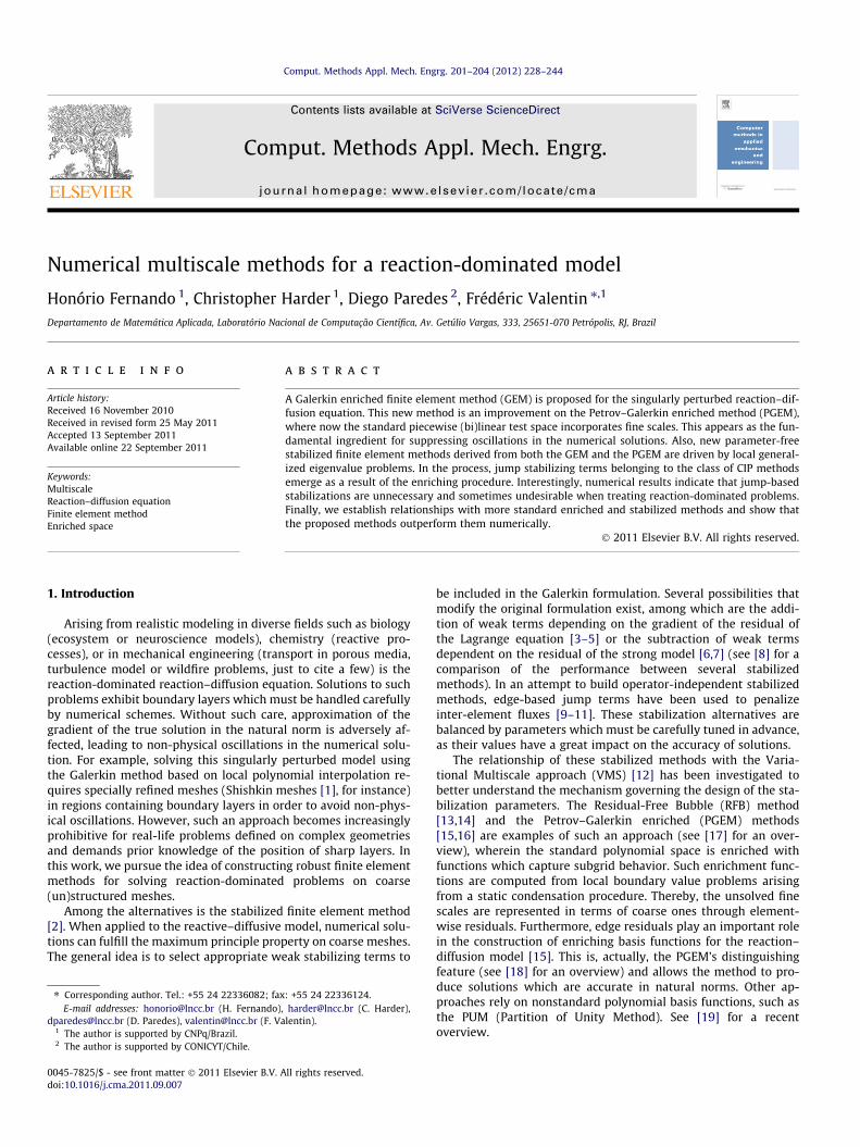
Fig. 1 illustrates such an example. The problem is set in the unitsquare, e = 10�6, r = 1, and f = 1 with homogenous Dirichlet bound-ary conditions. The solution shows a boundary layer region whichis badly approached due to the small scale in e relative to the meshsize. Indeed, the linear basis functions are ignorant of the boundarylayer in the true solution which occurs within the cells. The numer-ical solution therefore displays a poor approximation on boundarycells which is then manifested as a series of oscillations moving
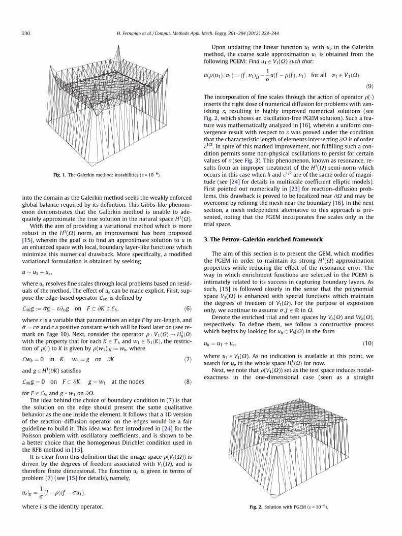
Fig. 1. The Galerkin method: instabilities (e = 10�6).
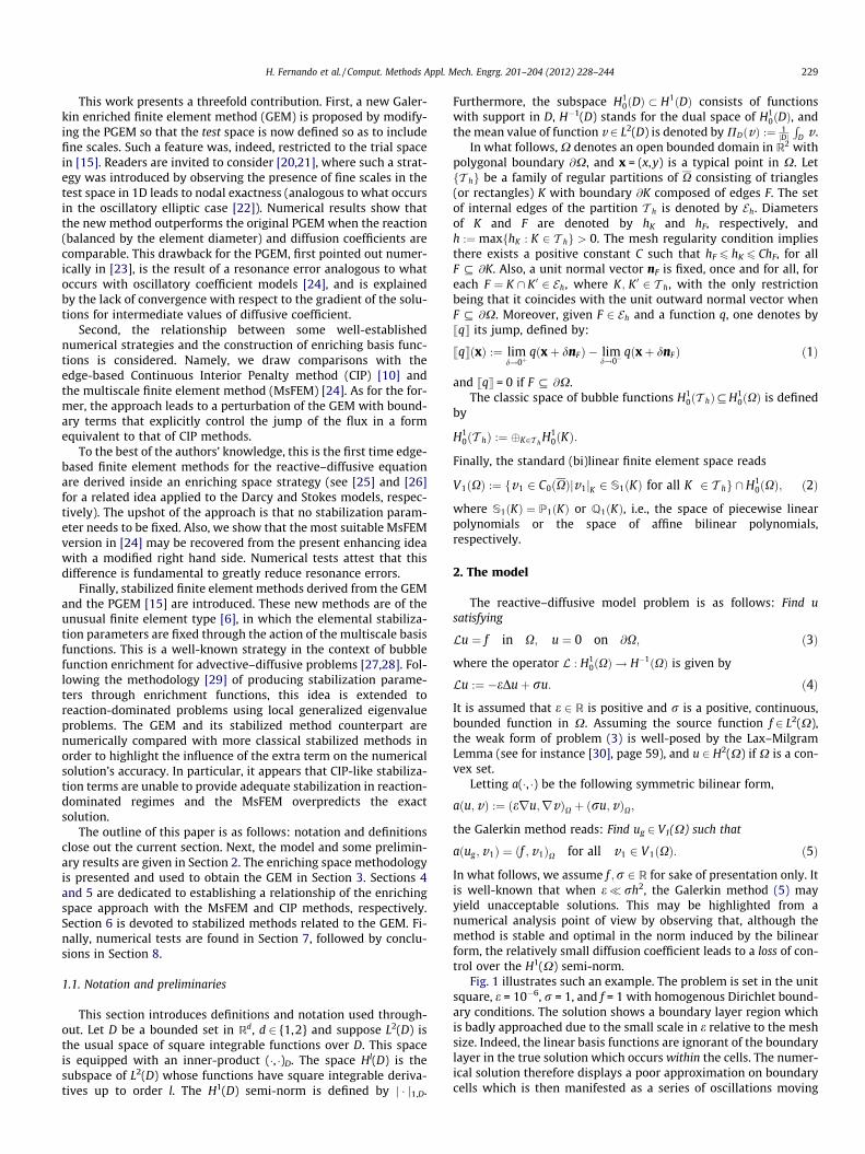
Fig. 2. Solution with PGEM (e = 10�6).
230 H. Fernando et al. / Comput. Methods Appl. Mech. Engrg. 201–204 (2012) 228–244
into the domain as the Galerkin method seeks the weakly enforcedglobal balance required by its definition. This Gibbs-like phenom-enon demonstrates that the Galerkin method is unable to ade-quately approximate the true solution in the natural space H1(X).
With the aim of providing a variational method which is morerobust in the H1(X) norm, an improvement has been proposed[15], wherein the goal is to find an approximate solution to u inan enhanced space with local, boundary layer-like functions whichminimize this numerical drawback. More specifically, a modifiedvariational formulation is obtained by seeking
u � u1 þ ue;
where ue resolves fine scales through local problems based on resid-uals of the method. The effect of ue can be made explicit. First, sup-pose the edge-based operator L@K is defined by
L@K g :¼ �rg � e@ssg on F � @K 2 Eh; ð6Þ
where s is a variable that parametrizes an edge F by arc-length, and�r ¼ cr and c a positive constant which will be fixed later on (see re-mark on Page 10). Next, consider the operator q : V1ðXÞ ! H1
0ðXÞwith the property that for each K 2 T h and w1 2 S1ðKÞ, the restric-tion of q(�) to K is given by q(w1)jK :¼ wh, where
Lwh ¼ 0 in K; wh ¼ g on @K ð7Þ
and g 2 H1(@K) satisfies
L@K g ¼ 0 on F � @K; g ¼ w1 at the nodes ð8Þ
for F 2 Eh, and g = w1 on @X.The idea behind the choice of boundary condition in (7) is that
the solution on the edge should present the same qualitativebehavior as the one inside the element. It follows that a 1D versionof the reaction–diffusion operator on the edges would be a fairguideline to build it. This idea was first introduced in [24] for thePoisson problem with oscillatory coefficients, and is shown to bea better choice than the homogenous Dirichlet condition used inthe RFB method in [15].
It is clear from this definition that the image space q(V1(X)) isdriven by the degrees of freedom associated with V1(X), and istherefore finite dimensional. The function ue is given in terms ofproblem (7) (see [15] for details), namely,
uejK ¼1rðI � qÞðf � ru1Þ;
where I is the identity operator.
Upon updating the linear function u1 with ue in the Galerkinmethod, the coarse scale approximation u1 is obtained from thefollowing PGEM: Find u1 2 V1(X) such that:
aðqðu1Þ;v1Þ ¼ ðf ;v1ÞX �1r
aðf �qðf Þ;v1Þ for all v1 2 V1ðXÞ:
ð9Þ
The incorporation of fine scales through the action of operator q(�)inserts the right dose of numerical diffusion for problems with van-ishing e, resulting in highly improved numerical solutions (seeFig. 2, which shows an oscillation-free PGEM solution). Such a fea-ture was mathematically analyzed in [16], wherein a uniform con-vergence result with respect to e was proved under the conditionthat the characteristic length of elements intersecting @X is of ordere1/2. In spite of this marked improvement, not fulfilling such a con-dition permits some non-physical oscillations to persist for certainvalues of e (see Fig. 3). This phenomenon, known as resonance, re-sults from an improper treatment of the H1(X) semi-norm whichoccurs in this case when h and e1/2 are of the same order of magni-tude (see [24] for details in multiscale coefficient elliptic models).First pointed out numerically in [23] for reaction–diffusion prob-lems, this drawback is proved to be localized near @X and may beovercome by refining the mesh near the boundary [16]. In the nextsection, a mesh independent alternative to this approach is pre-sented, noting that the PGEM incorporates fine scales only in thetrial space.
3. The Petrov–Galerkin enriched framework
The aim of this section is to present the GEM, which modifiesthe PGEM in order to maintain its strong H1(X) approximationproperties while reducing the effect of the resonance error. Theway in which enrichment functions are selected in the PGEM isintimately related to its success in capturing boundary layers. Assuch, [15] is followed closely in the sense that the polynomialspace V1(X) is enhanced with special functions which maintainthe degrees of freedom of V1(X). For the purpose of expositiononly, we continue to assume r; f 2 R in X.
Denote the enriched trial and test spaces by Vh(X) and Wh(X),respectively. To define them, we follow a constructive processwhich begins by looking for uh 2 Vh(X) in the form
uh ¼ u1 þ ue; ð10Þ
where u1 2 V1(X). As no indication is available at this point, wesearch for ue in the whole space H1
0ðXÞ for now.Next, we note that q(V1(X)) set as the test space induces nodal-
exactness in the one-dimensional case (seen as a straight
Fig. 3. Solution with PGEM (e = 10�4).
H. Fernando et al. / Comput. Methods Appl. Mech. Engrg. 201–204 (2012) 228–244 231
adaptation of Remark 4.2 in [22] to the present case). Hence, we se-lect q(V1(X)) (instead of V1(X) as in [15]) to be enhanced withfunctions with local support in each K 2 T h; thereby, a static con-densation procedure can be employed. In other words, the testspace Wh(X) incorporates fine scales and is defined by
WhðXÞ :¼ qðV1ðXÞÞ � H10ðT hÞ: ð11Þ
Accordingly, an element vh 2Wh(X) may be decomposed as
vh ¼ qðv1Þ þ vb;
where v1 2 V1(X) and vb 2 H10ðT hÞ.
The associated Petrov–Galerkin formulation then reads: Finduh 2 Vh(X) such that
aðuh; vhÞ ¼ ðf ;vhÞX for all vh 2WhðXÞ: ð12Þ
Using the decomposition (11) in the definition of space Wh(X),uh 2 Vh(X) clearly satisfies the equivalent system:
aðuh;qðv1ÞÞ ¼ ðf ;qðv1ÞÞX for all v1 2 V1ðXÞ; ð13Þaðuh; vK
b ÞK ¼ ðf ; vKb ÞK for all vK
b 2 H10ðKÞ: ð14Þ
Integrating (14) by parts, together with the condition vKb j@K ¼ 0 and
Du1 = 0, shows the function ue satisfies
Lue ¼ f � ru1 in each K 2 T h: ð15Þ
As the local operator inside elements is fixed, we are now left toprescribe boundary conditions for it. Uniqueness is assured for(15) by prescribing a non-homogenous Dirichlet boundary condi-tion on internal edges given as follows:
ue ¼ g on F � @K n @X ð16Þ
and ue = 0 on @X, where g 2 H1(@K) satisfies
L@K g ¼�rrðf � ru1Þ on F; g ¼ 0 at the nodes: ð17Þ
Remark. At this point, we can revisit Vh(X) and refine itsdefinition as follows
VhðXÞ :¼ V1ðXÞ
� ve 2 H10ðXÞ : vejK ¼
1rðI � qÞðf � rv1Þ; v1 2 V1ðXÞ
� �;
which is a finite dimensional space since f 2 R is fixed and V1(X) isfinite dimensional. h
From Eqs. (15) and (16), it holds that ue is computed with re-spect to f and the degrees of freedom of its coarse-scale counter-part u1. Following this observation, it is convenient to splitue ¼ u1
e þ ufe and g = g1 + gf, where each contribution satisfies,
Lu1e ¼ �ru1 in K; u1
e ¼ g1 on @K; ð18ÞL@K g1 ¼ ��ru1 on F � @K; g1 ¼ 0 at the nodes ð19Þ
and
Lufe ¼ f in K; uf
e ¼ gf on @K; ð20Þ
L@K gf ¼�rr
f on F � @K gf ¼ 0 at the nodes: ð21Þ
Now, using f 2 R, a closed form for the solutions of (18)–(21) isavailable and given in terms of the operator q(�) defined in (7) and(8). In fact, it holds
ufe ¼
1rðf � qðf ÞÞ and u1
e ¼ qðu1Þ � u1: ð22Þ
Using the characterization above, we arrive at
aðuh;qðv1ÞÞ ¼ aðu1 þ u1e ;qðv1ÞÞ þ aðuf
e;qðv1ÞÞ¼ aðqðu1Þ;qðv1ÞÞ þ aðuf
e;qðv1ÞÞ: ð23Þ
Gathering this together with the observation
aðufe;qðv1ÞÞ ¼ ðf ;qðv1ÞÞX �
1r
aðqðf Þ;qðv1ÞÞ;
the GEM follows from (13) and reads: Find u1 2 V1(X) such that
aðqðu1Þ;qðv1ÞÞ ¼1r
aðqðf Þ;qðv1ÞÞ for all v1 2 V1ðXÞ: ð24Þ
Relaxing the assumptions on f and r makes the characterizationfor uf
e in (22) no longer valid. In such a case, the GEM is obtainedreplacing (23) in (13), which gives
aðqðu1Þ;qðv1ÞÞ ¼ ðf ;qðv1ÞÞ � aðufe;qðv1ÞÞ for all v1 2 V1ðXÞ;
ð25Þ
where ufe satisfies (20) and must be approached through a two-level
method. Observe that (24) (or (25)) reflects the effect of the enhanc-ing methodology (12), leading to a redesign of the basis functions.
Remarks.
� The difference between the PGEM (9) and the GEM (24) is thespace of test functions. Whereas the test functions are (bi)linearfor the former, multiscale aspects are incorporated in the latter.The numerical tests in Section 7 indicate this is key to minimiz-ing the resonance error.� The efficiency of method (24) arises from the ability to solve
local problems (15) and (16) analytically (as opposed to atwo-level approach [31]). Indeed, thanks to the linearity ofoperators L and L@K , what is needed is q(wi), where wi repre-sents the (bi)linear basis function associated with node i. Fol-lowing [15,16], a closed formula is made available byselecting the constant c appropriately in (16). On triangularmeshes and rectilinear rectangular meshes, respectively, thefollowing results hold:
qðwiÞ :¼ sinhðaKwiÞsinhðaKÞ
and
qðwiÞ :¼ sinhðaxKwx
i Þsinhðax
KÞsinhðay
Kwyi Þ
sinhðayKÞ
; ð26Þ
where wxi ðxÞw
yi ðyÞ defines the bilinear basis functions and
aK :¼ffiffiffiffiffiffi�rh2
Ke
q; ax
K :¼ffiffiffiffiffiffi�rh2
xe
q; ay
K :¼ffiffiffiffiffiffi�rh2
y
e
q, and hx and hy are the edge
lengths of the rectangle K. We recall that �r :¼ cr, and then, c
232 H. Fernando et al. / Comput. Methods Appl. Mech. Engrg. 201–204 (2012) 228–244
equals 12 for the rectilinear rectangular element, for example (see
[15] for the exact value of c in the triangle element case).� Once u1 is computed from (24), the enriching function ue is given
analytically using the basis functions q(wi). It is then easy to cal-culate uh, which satisfies the point-wise conservation property
Luh ¼ f in each K:
For rough f 2 H1(X), the enriching function ufe must be approxi-
mated by a two level method. However, this extra computationmay be avoided by replacing uf
e by �ufe defined as the solution of
(20) and (21), where the right-hand side is given by PK(f). Then,�uf
e rather than ufe is used in the GEM to obtain the solution �u1.
Using (15) and (16), the result is qð�u1Þ þ �ufe, which satisfies the
local conservation property
ZKLðqð�u1Þ þ �ufeÞ ¼Z
Kf in each K 2 T h;
without impacting accuracy. It is also worth pointing out that,unlike discontinuous Galerkin methods [32], the stated local con-servation properties are reached with the relatively low cost of acontinuous method.� The boundary condition (16) implies uh is a conforming approx-
imation of u, i.e.,
suhtjF ¼ 0 for all F 2 Eh and uhj@X ¼ u1;
once c in �r is uniquely prescribed on each F 2 Eh. Thereby, thebasis functions (26) match on edges when quadrilateral andequilateral triangular meshes are used, and we assume thisholds from now on. Furthermore, integrating Eq. (13) by parts,and using characterization (15) for ue, it holdsXF2Eh
ðesruh � nt;qðv1ÞÞF ¼XK2T h
ðLuh � f ;qðv1ÞÞK
þX
K
ðeruh � n;qðv1ÞÞ@K
¼ aðuh;qðv1ÞÞ � ðf ;qðv1ÞÞX ¼ 0:
Thus, the continuity of the flux is weakly imposed. This is thetype of continuity enforcement which drives the constructionof discontinuous Galerkin methods (see [33] for an interestingviewpoint).� Problems with varying r and e are handled analytically by solv-
ing problems (18)–(21) where PK(r) and PK(e) replace the ori-ginal reactive and diffusive coefficients. No loss of accuracy isexpected as the consistency error relies on the approximationproperty of PK(�) and, thus, does not affect convergence proper-ties of the method. As for the 3D extension, we may adapt theboundary condition constant c and still propose the use of thebasis functions q(wi) given above. We point out that in bothcases the modification is concerned with the redesign of aK
only. h
4. Relationship with the MsFEM
Recall the observation that the space q(V1(X)) as defined by (7)is finite dimensional, consisting of basis functions taking degrees offreedom of V1(X). Observing this basis contains subgrid informa-tion, [24,22] introduced the Multiscale Finite Element Method(MsFEM): Find u1 2 V1(X) such that
aðqðu1Þ;qðv1ÞÞ ¼ ðf ;qðv1ÞÞ for all v1 2 V1ðXÞ ð27Þ
for the case that e is a function with multiple scales and r = 0. It isinteresting to study how a method of this form performs when ex-tended to a highly reactive reaction–diffusion equation, and howthis performance compares to the GEM (24).
In fact, the GEM is closely related to this method in form. We re-call from (25) that the GEM reads: Find u1 2 V1(X) such that
aðqðu1Þ;qðv1ÞÞ ¼ ðf ;qðv1ÞÞ � aðufe;qðv1ÞÞ for all v1 2 V1ðXÞ:
ð28Þ
To better understand the effect of the term on the right-hand side,decompose (20) and (21) as uf
e ¼ ~ufe þ uf
e, where
L~ufe ¼ f in K; ~uf
e ¼ 0 on @K
and
Lufe ¼ 0 in K; uf
e ¼ gf on @K; ð29Þ
L@K gf ¼�rr f on F � @K; gf ¼ 0 at the nodes: ð30Þ
By definition (7) of q(v1) and the fact that ~ufe 2 H1
0ðT hÞ, weobtain
að~ufe;qðv1ÞÞ ¼ 0;
so that (28) becomes
aðqðu1Þ;qðv1ÞÞ¼ðf ;qðv1ÞÞ�aðufe;qðv1ÞÞ for all v1 2V1ðXÞ: ð31Þ
This clearly shows that the portion of the element-based residualassociated with the source term has no impact on the GEM. As itstands, the nonzero boundary condition in (29) implies an extracontribution to the GEM over that which is present in the MsFEMextended to the reaction–diffusion equation. In fact, integrationby parts, applying Eq. (29), and using the continuity of q(v1) implies
aðufe;qðv1ÞÞ ¼
XF2Eh
ðesrufe � nt;qðv1ÞÞF :
Therefore, the ultimate contribution of ufe is the penalization of
jumps of the gradient on internal edges. This result is consistentwith the remark in Section 3 regarding the observation that theGEM may be reduced to a method which imposes the weak continu-ity of the flux on internal edges. Numerical tests in Section 7 explorethe effect of this edge-based contribution by drawing comparisonsbetween the GEM and the MsFEM extended to the reaction–diffu-sion equation.
Remark. In [24,22] another version of the MsFEM was introducedwhere the functions are assumed to vary linearly on internal edges.This has been compared to the RFB method [34], where thedifference arises in the RFB’s calculation of local enrichmentsrelated to the source term. As this term does not appear explicitlyin the coarse problem, the RFB and MsFEM are equivalent in thiscase. However, numerical results in [15] have shown that the RFBmethod lacks precision when applied to reaction-dominatedproblems. h
5. Recovering a CIP method
CIP methods have been used to stabilize singularly perturbedmodels, with an emphasis placed on highly advective problems.Although it has been claimed that they may be made to work inthe reaction-dominated regime as well, to the best of the authors’knowledge no CIP method has been numerically verified for thiscase. Bearing this in mind, the enriched approach presented inthe last section may be used to derive new methods which, in par-ticular cases, have a CIP-like form.
To this end, and mimicking the enriching procedure used to de-rive the GEM (24), consider the modified boundary condition forlocal problem (15) which penalizes the jump of the flux acrossinternal edges:

H. Fernando et al. / Comput. Methods Appl. Mech. Engrg. 201–204 (2012) 228–244 233
ue ¼ g on F 2 Eh ð32Þ
and ue = 0 on @X, where g satisfies
L@K g ¼�rrðf � ru1Þ þ
ehF
sru1 � nt on F � @K; g
¼ 0 at the nodes: ð33Þ
This choice agrees with the a posteriori error estimators proposedfor elliptic problems in [35], wherein the jump of the flux is inter-preted as the residual across edges. Consequently, the function ue
now incorporates an enriching contribution, denoted uJe, which
accounts for the jump of the flux and solves
LuJe ¼ 0 in K; uJ
e ¼ gJ on @K; ð34Þ
L@K gJ ¼e
hFsru1 � nt on F � @K; gJ ¼ 0 at the nodes: ð35Þ
Computed from (18)–(21) and (34) and (35), the redefined ue
still fulfills Eq. (14). The boundary condition gJ may be rewrittenas gJ ¼ bF
ehF
sru1 � nt, where an analytic expression for bF is easilyobtained by solving
L@K bF ¼ 1 on F � @K; bF ¼ 0 at nodes: ð36Þ
From (7), Lqðv1Þ ¼ 0 in each K, which indicates the contribution ofuJ
e in the method may be rewritten as
aðuJe;qðv1ÞÞ ¼
XK2T h
ðuJe;Lqðv1ÞÞK þ
XK2T h
ðuJe; erqðv1Þ � nÞ@K
¼XF2Eh
ðgJ ; esrqðv1Þ � ntÞF
¼XF2Eh
ehFðbFsru1 � nt; esrqðv1Þ � ntÞF : ð37Þ
The characterization above yields an alternative version of theGEM with an explicit control on the flux across internal edges: Findu1 2 V1(X) such that
Bðu1;v1Þ ¼ Fðv1Þ for all v1 2 V1ðXÞ; ð38Þ
with
Bðu1;v1Þ :¼ aðqðu1Þ;qðv1ÞÞ þXF2Eh
ehFðbFsru1 � nt; esrqðv1Þ � ntÞF ;
Fðv1Þ :¼ 1r
aðqðf Þ;qðv1ÞÞ;
where bF solves (36).
Remark. Similarly, the PGEM of [15] may be updated with thejump-dependent enrichment (34) and (35), which leads to analternative PGEM. Following (37), with v1 replacing test functions
–10
0.00020.00040.00060.0008
0.0010.00120.0014
Fig. 4. Value of sK (left) and its correspondin
q(v1), and neglecting the termP
K2T hðuJ
e;rv1ÞK , this alternativePGEM with flux control on the edges reads: Find u1 2 V1(X) suchthat
BFMV ðu1;v1Þ ¼ FFMV ðv1Þ for all v1 2 V1ðXÞ; ð39Þ
with
BFMV ðu1;v1Þ :¼ aðqðu1Þ;v1Þ þXF2Eh
sFðsru1 � nt; esrv1 � ntÞF ;
FFMV ðv1Þ :¼ 1r
aðqðf Þ; v1Þ;
where, given aF :¼ffiffiffiffiffiffi�rh2
Fe
q; sF stands for
sF ¼e
hFPFðbFÞ ¼
1a2
F
2hFð1� coshðaFÞÞaF sinhðaFÞ
þ hF
� �: ð40Þ
The new method (39) contains an edge-based CIP term which is bal-anced by a parameter sF with no free constant (unlike the standardCIP term). The influence of edge-based stabilization on the numer-ical solutions for both (39) and a standard CIP method is explorednumerically in Section 7. h
6. Recovering unusual stabilized methods
Methods (9), (24), (38) and (39) possess terms which may havelarge gradients in the presence of boundary or internal layers. Assuch, special numerical quadratures [36] (or exact integration)are required to ensure their good performance. With the goal ofavoiding the more involved numerical integration without losingaccuracy, this section presents stabilized methods which are for-mally derived from the GEM (24).
Assume that the following approximation holds, K 2 T h,
ðqðw1Þ;qðv1ÞÞK � rkKmaxðw1;v1ÞK v1;w1 2 S1ðKÞ; ð41Þ
where rkKmax 2 ð0;1Þ is the largest generalized eigenvalue l related
to the generalized eigenvalue problem Aw = lBw. The entries of thesymmetric positive definite matrices A and B are [Aji] = (q(-wi),q(wj))K and [Bji] = (wi,wj)K, respectively. We recall that wi arethe standard (bi)linear basis for S1ðKÞ. Furthermore, suppose
eðrqðw1Þ;rqðv1ÞÞK � eðrw1;rv1ÞK v1;w1 2 S1ðKÞ: ð42Þ
Using approximations (41) and (42) with, alternatively, w1 = u1
and w1 = f, and replacing them in (24), the following stabilizedmethod arises: Find u1 2 V1(X) such that
Bsðu1;v1Þ ¼ Fsðv1Þ for all v1 2 V1ðXÞ; ð43Þ
–1
–0.5
0
0.5
1
x
–0.5
0
0.5
1
y
g enriching function (right). Here aK = 1.

–1
–0.5
0
0.5
1
x
–1
–0.5
0
0.5
1
y
0
0.2
0.4
0.6
0.8
1
Fig. 5. Value of sK (left) and its corresponding enriching function (right). Here aK = 10.
–1
–0.5
0
0.5
1
x
–1
–0.5
0
0.5
1
y
0
0.2
0.4
0.6
0.8
1
Fig. 6. Value of sK (left) and its corresponding enriching function (right). Here aK = 25.
234 H. Fernando et al. / Comput. Methods Appl. Mech. Engrg. 201–204 (2012) 228–244
where
Bsðu1;v1Þ :¼ aðu1;v1Þ �XK2T h
sKðru1;rv1ÞK ;
Fsðv1Þ :¼ ðf ;v1Þ �XK2T h
sKðf ;rv1ÞK :
The parameter sK :¼ 1r ð1� rkK
maxÞ reads
sK ¼
1r 1� 6ð4 coshðaK ÞþcoshðaK Þ2�2aK sinhðaK Þ�a2
K�5ÞðaK sinhðaK ÞÞ2
h i
for triangles;
1r 1� 3ðsinhðaK Þ2�a2
K ÞðaK sinhðaK ÞÞ2
h ifor quadrangles:
8>>>><>>>>:
ð44Þ
A stabilized method starting from the PGEM (9) arises byassuming equivalent simplifications. This leads to the followingstabilized method: Find u1 2 V1(X) such that
BsFMV ðu1; v1Þ ¼ Fs
FMVðv1Þ for all v1 2 V1ðXÞ; ð45Þ
where
BsFMVðu1;v1Þ :¼ aðu1; v1Þ �
XK2T h
~sKðru1;rv1ÞK ;
FsFMVðv1Þ :¼ ðf ;v1Þ �
XK2T h
~sKðf ;rv1ÞK ;
with the piecewise function ~sK now reading
~sK ¼1r 1� 6ðsinhðaK Þ�aK Þ
a2K sinhðaK Þ
� �for triangles;
1r 1� 4ðcoshðaK Þ�1Þ
a2Kð1þcoshðaK ÞÞ
� �for quadrangles:
8><>:
This version differs from (43) only in the definition of the elementalstabilization parameter. Figs. 4–6 illustrate the impact variousvalues for aK have on the enriching function wi � q(wi) (picturedon a patch of four triangles) and the value of sK given in (44).
Remarks.
� By following closely the equivalence result in Lemma 1 in[16] we can establish that (37) holds in the particular casew1 = v1, i.e. the norms induced by the bilinear forms areequivalent on the discrete space. The analysis of the errorinvolved is not pursued here, though it will be addressed ina forthcoming work. For now, it is assumed that approxima-tions (41) and (42) hold in the sense that the associated erroris of the order of leading error estimates. This assumption isnumerically verified in Section 7, wherein solutions from (24)(or (9)) and (43) (or (45)) are shown to stay ‘‘close’’.
� Using the approximation strategy in the jump-based versionof the GEM (38), together with the assumption
ehFðbFsru1 � nt; esrqðv1Þ � ntÞF
� ehFðbFsru1 � nt; esrv1 � ntÞF ; ð46Þ
the bilinear form Bs(�, �) in (43) includes the following:
XF2EhsFðsru1 � nt; esrv1 � ntÞF ; ð47Þ
where sF is given in (40). The same extra term also appearswhen applying the approximation strategy to the jump-basedversion of PGEM (45). However, assumption (46) is no
0 0.1 0.2 0.3 0.4 0.5 0.6 0.7 0.8 0.9 10
0.2
0.4
0.6
0.8
1
GEMPGEMGALERKIN
0.75 0.8 0.85 0.9 0.95 10.9
0.92
0.94
0.96
0.98
1
1.02
1.04
1.06
1.08
1.1
GEMPGEMGALERKIN
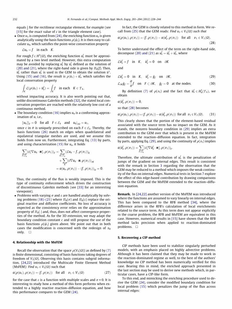
Fig. 7. Solutions from the PGEM and the GEM (top) and profile of solutions from the Galerkin method, the PGEM and the GEM at x = 0.5 (bottom left). Zoom of the curves(bottom right). Here e = 10�4.
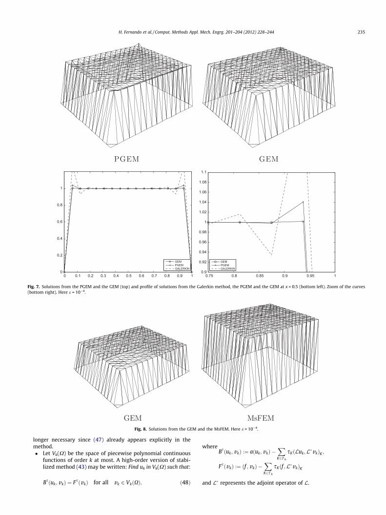
Fig. 8. Solutions from the GEM and the MsFEM. Here e = 10�4.
H. Fernando et al. / Comput. Methods Appl. Mech. Engrg. 201–204 (2012) 228–244 235
longer necessary since (47) already appears explicitly in themethod.� Let Vk(X) be the space of piecewise polynomial continuous
functions of order k at most. A high-order version of stabi-lized method (43) may be written: Find uk in Vk(X) such that:
Bsðuk;vkÞ ¼ FsðvkÞ for all vk 2 VkðXÞ; ð48Þ
wheres
X
B ðuk; vkÞ :¼ aðuk;vkÞ �K2T h
sKðLuk;L vkÞK ;
FsðvkÞ :¼ ðf ; vkÞ �XK2T h
sKðf ;LvkÞK
and L represents the adjoint operator of L.
0 0.1 0.2 0.3 0.4 0.5 0.6 0.7 0.8 0.9 10
0.5
1
1.5
2
GEMPGEM
Fig. 9. Profiles of solution from GEM and MsFEM at x = 0.5 Here e = 10�4.
236 H. Fernando et al. / Comput. Methods Appl. Mech. Engrg. 201–204 (2012) 228–244
� Method (43), together with (47), comprises of stabilizationingredients from the unusual [6] and the edge-based stabi-lized methods [10]. This is accomplished by the new designof elemental and edge stabilization parameters based on theenriching functions. Therefore, the method handles both thediffusive and the reactive limits continuously, with rsK and
Fig. 10. Solution from the new stabilized
Fig. 11. Solutions from the USFEM (left) an
rsF vanishing for the former case and tending to oneotherwise.
� All stabilized methods which have been presented are easilyextended to 3D cases by redefining aK with respect to thecharacteristic length of tetrahedrons (or hexahedrons). Themethods also handle problems with variable physical coeffi-cients by changing the value of aK so that it is defined in termsof PK(e) and PK(r). This last claim is numerically verified inSection 7. h
7. Numerical validations
With a series of three numerical tests, the GEM (24), its stabi-lized counterpart (43) (SGEM), and the stabilized version (45) ofthe PGEM (9) (denoted SPGEM) are shown to offer competitive,and often superior, results when compared with existing methods.All tests are performed on the unit square, which is partitioned intoboth structured (either triangles and rectangles) and unstructuredtriangular meshes. In particular, it is interesting to determine theeffect of e1=2 ¼ OðhÞ as this has been shown to produce a localizedresonance phenomenon [16,23] for the PGEM method (9) (seeFig. 3). Comparisons are made to four existing methods: 1) thePGEM (9), 2) the unusual stabilized finite element method (USFEM)of [6], 3) the CIP method of [10], and 4) the MsFEM (27). For thesake of completeness, the USFEM and the CIP methods are recalled.
The USFEM is: Find u1 2 V1(X) such that
methods (45) and (43). Here e = 10�4.
d the CIP (right) methods. Here 10�4.
10−7 10−6 10−5 10−4 10−30.9
1
1.1
1.2
1.3
1.4
1.5
1.6
1.7
1.8GALERKINGEMPGEMCIP
10−7 10−6 10−5 10−4 10−30.9
1
1.1
1.2
1.3
1.4
1.5
1.6GALERKINGEMPGEMCIP
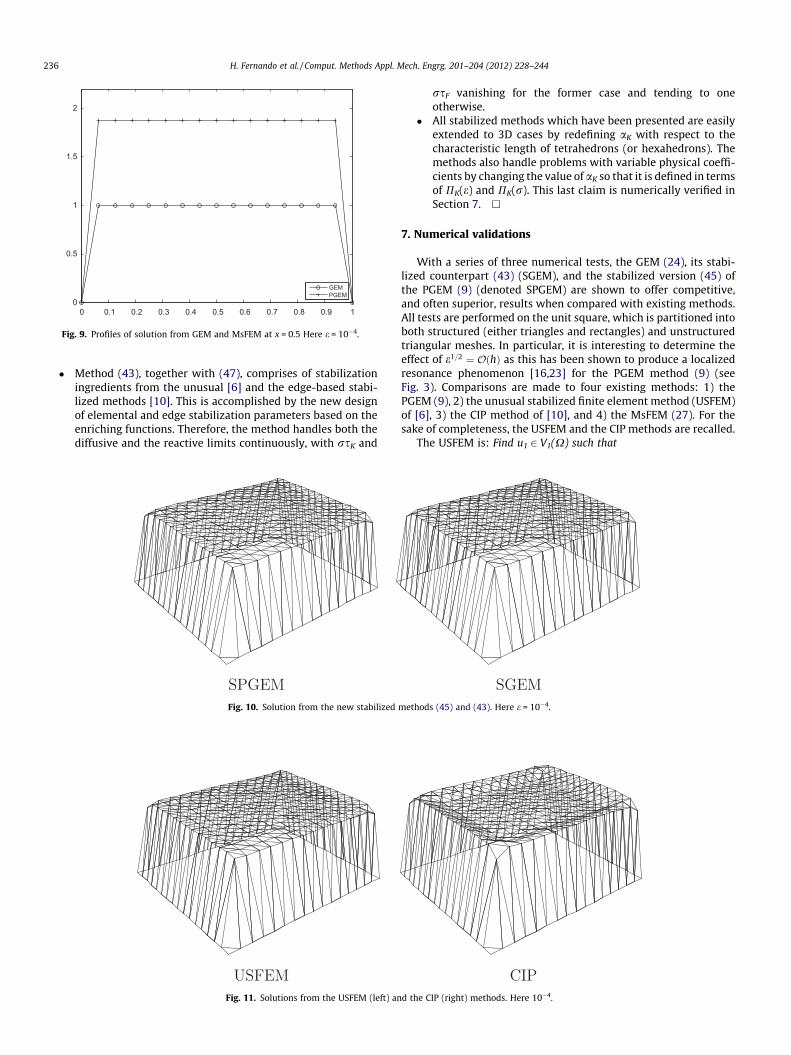
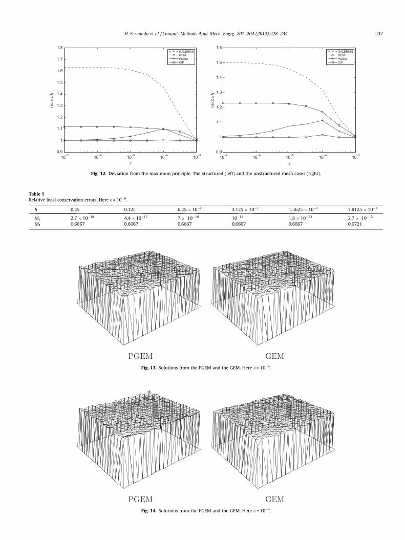
Fig. 12. Deviation from the maximum principle. The structured (left) and the unstructured mesh cases (right).
Table 1Relative local conservation errors. Here e = 10�6.
h 0.25 0.125 6.25 10�2 3.125 10�2 1.5625 10�2 7.8125 10�3
Me 2.7 10�18 4.4 10�17 7 10�16 10�14 1.8 10�13 2.7 10�12
M1 0.6667 0.6667 0.6667 0.6667 0.6667 0.6721
Fig. 13. Solutions from the PGEM and the GEM. Here e = 10�6.
Fig. 14. Solutions from the PGEM and the GEM. Here e = 10�4.
H. Fernando et al. / Comput. Methods Appl. Mech. Engrg. 201–204 (2012) 228–244 237
238 H. Fernando et al. / Comput. Methods Appl. Mech. Engrg. 201–204 (2012) 228–244
aðu1; v1Þ �XK2T h
sUSFEMK ðru1;rv1ÞK
¼ ðf ;v1ÞX �XK2T h
sUSFEMK ðf ;rv1ÞK ; for all v 2 V1ðXÞ ð49Þ
where sUSFEMK reads
sUSFEMK :¼ h2
K
rh2K max 1;aUSFEM
K
þ 6e
and aUSFEMK :¼ 6e
rh2K.
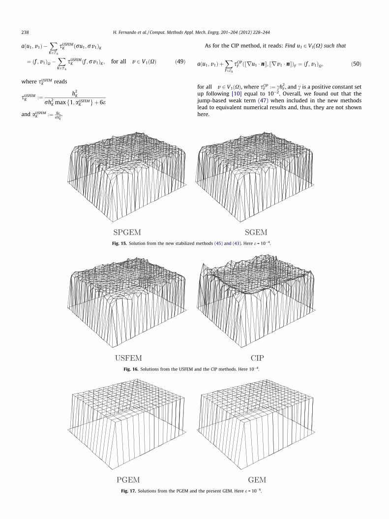
Fig. 15. Solution from the new stabilized
Fig. 16. Solutions from the USFEM a
Fig. 17. Solutions from the PGEM and
As for the CIP method, it reads: Find u1 2 V1(X) such that
aðu1;v1Þ þXF2Eh
sCIPF ðsru1 � nt; srv1 � ntÞF ¼ ðf ; v1ÞX; ð50Þ
for all v 2 V1ðXÞ, where sCIPF :¼ ch2
F , and c is a positive constant setup following [10] equal to 10�2. Overall, we found out that thejump-based weak term (47) when included in the new methodslead to equivalent numerical results and, thus, they are not shownhere.
methods (45) and (43). Here e = 10�4.
nd the CIP methods. Here 10�4.
the present GEM. Here e = 10�6.
H. Fernando et al. / Comput. Methods Appl. Mech. Engrg. 201–204 (2012) 228–244 239
7.1. The unit source problem
For this problem, the source f = 1, the reaction coefficientr = 1 and homogenous Dirichlet boundary conditions are pre-scribed. Consider first a structured mesh made up of triangles.When e = 1, all methods give similar results to the one fromthe Galerkin method.
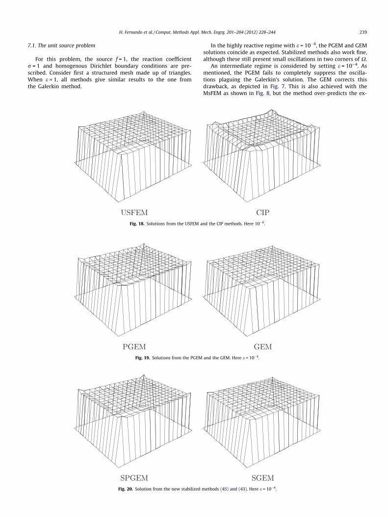
Fig. 18. Solutions from the USFEM a
Fig. 19. Solutions from the PGEM
Fig. 20. Solution from the new stabilized
In the highly reactive regime with e = 10�6, the PGEM and GEMsolutions coincide as expected. Stabilized methods also work fine,although these still present small oscillations in two corners of X.
An intermediate regime is considered by setting e = 10�4. Asmentioned, the PGEM fails to completely suppress the oscilla-tions plaguing the Galerkin’s solution. The GEM corrects thisdrawback, as depicted in Fig. 7. This is also achieved with theMsFEM as shown in Fig. 8, but the method over-predicts the ex-
nd the CIP methods. Here 10�6.
and the GEM. Here e = 10�4.
methods (45) and (43). Here e = 10�4.
0.0039 0.0078 0.0156 0.0312 0.0625 0.125 0.25
0.75
0.8
0.85
0.9
0.95
1
1.1
1.2
1.3
1.4
1.5
GEMGALERKIN
0.0039 0.0078 0.0156 0.0312 0.0625 0.125 0.25
0.75
0.8
0.85
0.9
0.95
1
GEMSGEMUNUSUALCIP
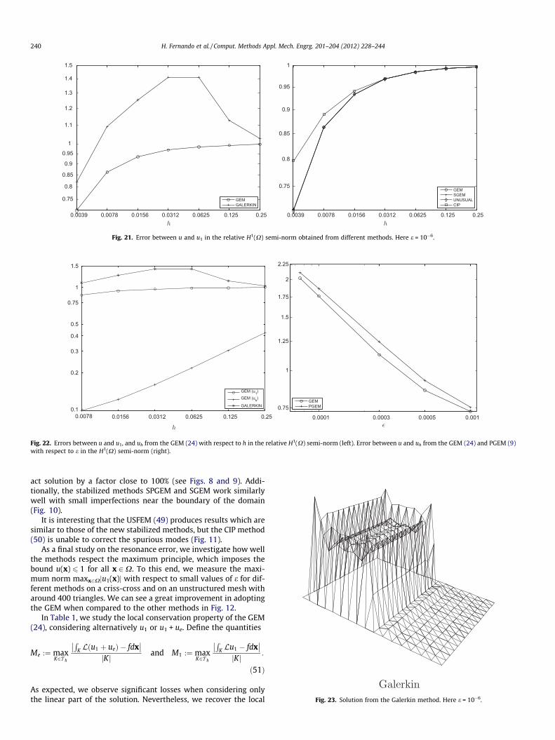
Fig. 21. Error between u and u1 in the relative H1(X) semi-norm obtained from different methods. Here e = 10�6.
0.0078 0.0156 0.0312 0.0625 0.125 0.250.1
0.2
0.3
0.4
0.5
0.75
1
1.5
h
GEM (u1)GEM (uh)
GALERKIN
0.0001 0.0003 0.0005 0.001
0.75
1
1.25
1.5
1.75
2
2.25
GEMPGEM
Fig. 22. Errors between u and u1, and uh from the GEM (24) with respect to h in the relative H1(X) semi-norm (left). Error between u and uh from the GEM (24) and PGEM (9)with respect to e in the H1(X) semi-norm (right).
Fig. 23. Solution from the Galerkin method. Here e = 10�6.
240 H. Fernando et al. / Comput. Methods Appl. Mech. Engrg. 201–204 (2012) 228–244
act solution by a factor close to 100% (see Figs. 8 and 9). Addi-tionally, the stabilized methods SPGEM and SGEM work similarlywell with small imperfections near the boundary of the domain(Fig. 10).
It is interesting that the USFEM (49) produces results which aresimilar to those of the new stabilized methods, but the CIP method(50) is unable to correct the spurious modes (Fig. 11).
As a final study on the resonance error, we investigate how wellthe methods respect the maximum principle, which imposes thebound u(x) 6 1 for all x 2X. To this end, we measure the maxi-mum norm maxx2Xju1(x)j with respect to small values of e for dif-ferent methods on a criss-cross and on an unstructured mesh witharound 400 triangles. We can see a great improvement in adoptingthe GEM when compared to the other methods in Fig. 12.
In Table 1, we study the local conservation property of the GEM(24), considering alternatively u1 or u1 + ue. Define the quantities
Me :¼maxK2T h
RK Lðu1 þ ueÞ � fdx
�� ��jKj and M1 :¼ max
K2T h
RK Lu1 � fdx
�� ��jKj :
ð51Þ
As expected, we observe significant losses when considering onlythe linear part of the solution. Nevertheless, we recover the local
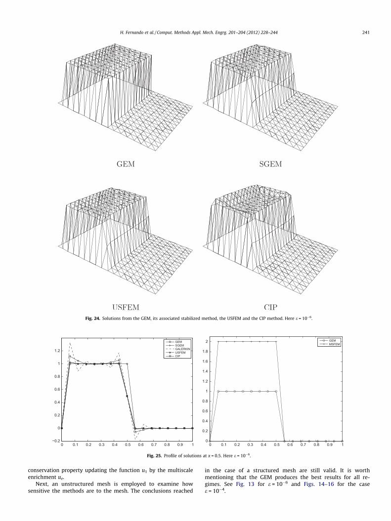
Fig. 24. Solutions from the GEM, its associated stabilized method, the USFEM and the CIP method. Here e = 10�6.
0 0.1 0.2 0.3 0.4 0.5 0.6 0.7 0.8 0.9 1−0.2
0
0.2
0.4
0.6
0.8
1
1.2
GEMSGEMGALERKINUSFEMCIP
0 0.1 0.2 0.3 0.4 0.5 0.6 0.7 0.8 0.9 10
0.2
0.4
0.6
0.8
1
1.2
1.4
1.6
1.8
2 GEMMSFEM
Fig. 25. Profile of solutions at x = 0.5. Here e = 10�6.
H. Fernando et al. / Comput. Methods Appl. Mech. Engrg. 201–204 (2012) 228–244 241
conservation property updating the function u1 by the multiscaleenrichment ue.
Next, an unstructured mesh is employed to examine howsensitive the methods are to the mesh. The conclusions reached
in the case of a structured mesh are still valid. It is worthmentioning that the GEM produces the best results for all re-gimes. See Fig. 13 for e = 10�6 and Figs. 14–16 for the casee = 10�4.
0 0.05 0.1 0.15 0.2 0.250.8
0.85
0.9
0.95
1
1.05
1.1
1.15
GEMSGEMGALERKINUSFEMCIP
0.4 0.45 0.5 0.55 0.6−0.2
0
0.2
0.4
0.6
0.8
1
GEMSGEMGALERKINUSFEMCIP
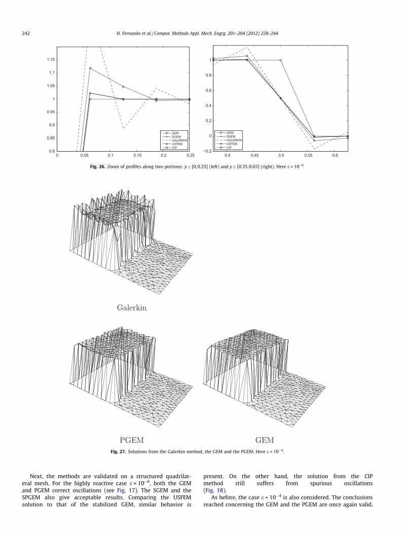
Fig. 26. Zoom of profiles along two portions: y 2 [0,0.25] (left) and y 2 [0.35,0.65] (right). Here e = 10�6.
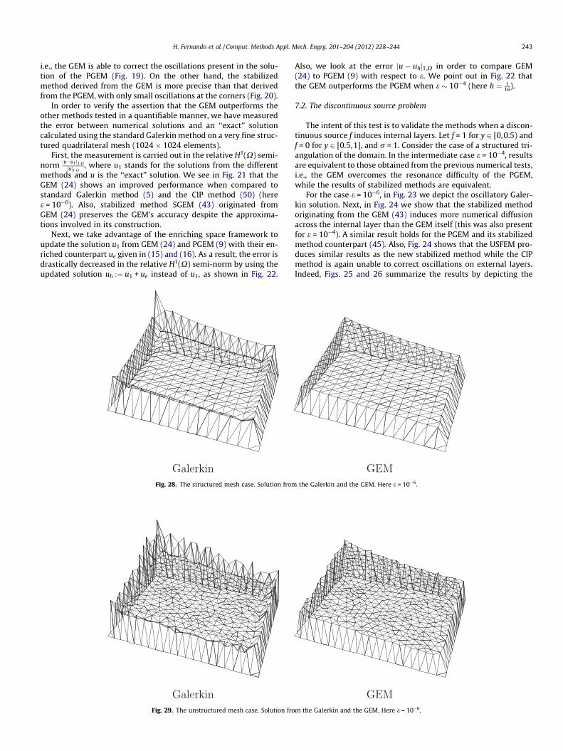
Fig. 27. Solutions from the Galerkin method, the GEM and the PGEM. Here e = 10�4.
242 H. Fernando et al. / Comput. Methods Appl. Mech. Engrg. 201–204 (2012) 228–244
Next, the methods are validated on a structured quadrilat-eral mesh. For the highly reactive case e = 10�6, both the GEMand PGEM correct oscillations (see Fig. 17). The SGEM and theSPGEM also give acceptable results. Comparing the USFEMsolution to that of the stabilized GEM, similar behavior is
present. On the other hand, the solution from the CIPmethod still suffers from spurious oscillations(Fig. 18).
As before, the case e = 10�4 is also considered. The conclusionsreached concerning the GEM and the PGEM are once again valid,
H. Fernando et al. / Comput. Methods Appl. Mech. Engrg. 201–204 (2012) 228–244 243
i.e., the GEM is able to correct the oscillations present in the solu-tion of the PGEM (Fig. 19). On the other hand, the stabilizedmethod derived from the GEM is more precise than that derivedfrom the PGEM, with only small oscillations at the corners (Fig. 20).
In order to verify the assertion that the GEM outperforms theother methods tested in a quantifiable manner, we have measuredthe error between numerical solutions and an ‘‘exact’’ solutioncalculated using the standard Galerkin method on a very fine struc-tured quadrilateral mesh (1024 1024 elements).
First, the measurement is carried out in the relative H1(X) semi-norm ju�u1 j1;X
juj1;X, where u1 stands for the solutions from the different
methods and u is the ‘‘exact’’ solution. We see in Fig. 21 that theGEM (24) shows an improved performance when compared tostandard Galerkin method (5) and the CIP method (50) (heree = 10�6). Also, stabilized method SGEM (43) originated fromGEM (24) preserves the GEM’s accuracy despite the approxima-tions involved in its construction.
Next, we take advantage of the enriching space framework toupdate the solution u1 from GEM (24) and PGEM (9) with their en-riched counterpart ue given in (15) and (16). As a result, the error isdrastically decreased in the relative H1(X) semi-norm by using theupdated solution uh :¼ u1 + ue instead of u1, as shown in Fig. 22.
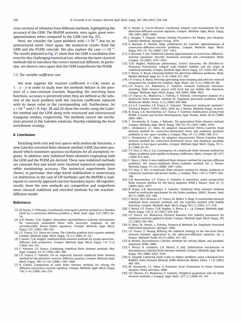
Fig. 28. The structured mesh case. Solution from
Fig. 29. The unstructured mesh case. Solution fro
Also, we look at the error ju � uhj1,X in order to compare GEM(24) to PGEM (9) with respect to e. We point out in Fig. 22 thatthe GEM outperforms the PGEM when e � 10�4 (here h ¼ 1
16).
7.2. The discontinuous source problem
The intent of this test is to validate the methods when a discon-tinuous source f induces internal layers. Let f = 1 for y 2 [0,0.5) andf = 0 for y 2 [0.5,1], and r = 1. Consider the case of a structured tri-angulation of the domain. In the intermediate case e = 10�4, resultsare equivalent to those obtained from the previous numerical tests,i.e., the GEM overcomes the resonance difficulty of the PGEM,while the results of stabilized methods are equivalent.
For the case e = 10�6, in Fig. 23 we depict the oscillatory Galer-kin solution. Next, in Fig. 24 we show that the stabilized methodoriginating from the GEM (43) induces more numerical diffusionacross the internal layer than the GEM itself (this was also presentfor e = 10�4). A similar result holds for the PGEM and its stabilizedmethod counterpart (45). Also, Fig. 24 shows that the USFEM pro-duces similar results as the new stabilized method while the CIPmethod is again unable to correct oscillations on external layers.Indeed, Figs. 25 and 26 summarize the results by depicting the
the Galerkin and the GEM. Here e = 10�6.
m the Galerkin and the GEM. Here e = 10�6.
244 H. Fernando et al. / Comput. Methods Appl. Mech. Engrg. 201–204 (2012) 228–244
cross sections of solutions from different methods, highlighting theaccuracy of the GEM. The MsFEM presents, once again, great over-approximation when compared to the GEM (see Fig. 25).
Next, we consider the same problem with e = 10�6, but on anunstructured mesh. Once again, the numerical results from theGEM and the PGEM coincide. We also explore the case e = 10�4.The results depicted in Fig. 27 show that the GEM is oscillation-freeeven for this challenging numerical test, whereas the more classicalmethods fail to introduce the correct numerical diffusion. In partic-ular, we observe once again that the GEM outperforms the PGEM.
7.3. The variable coefficient case
We now suppose the reaction coefficient r = r(x) varies as1 � x � y in order to study how the methods behave in the pres-ence of a non-constant reaction. Regarding the enriching basisfunctions, accuracy is preserved when they are defined as the solu-tion of the local problem with the reaction coefficient replacedwith its mean value in the corresponding cell. Furthermore, lete = 10�6 and f = 0. Figs. 28 and 29 show the results using the Galer-kin method and the GEM along with structured and unstructuredtriangular meshes, respectively. The methods correct the oscilla-tions present in the Galerkin solutions, thereby validating the localenrichment strategy.
8. Conclusion
Enriching both trial and test spaces with multiscale functions, anew Galerkin enriched finite element method (GEM) has been pro-duced which minimizes spurious oscillations for all asymptotic re-gimes. In addition, new stabilized finite elements originating withthe GEM and the PGEM are derived. These new stabilized methodsare constant-free and avoid more involved numerical integrationswhile maintaining accuracy. The numerical experiments haveshown, in particular, that edge-based stabilization is unnecessary(or deleterious in the case of CIP methods) and the MsFEM is inad-equate to correctly approach reactive boundary layers. All together,results show the new methods are competitive and outperformmore classical stabilized and enriched methods for the reaction–diffusion model.
References
[1] M. Stynes, E. O’Riordan, A uniformly convergent Galerkin method on a Shishkinmesh for a convection diffusion problem, J. Math. Anal. Appl. 214 (1997) 36–54.
[2] A.N. Brooks, T.J.R. Hughes, Streamline upwind/Petrov–Galerkin formulationsfor convection dominated flows with particular emphasis on theincompressible Navier–Stokes equations, Comput. Methods Appl. Mech.Engrg. (32) (1982) 199–259.
[3] L.P. Franca, E.G. Dutra do Carmo, The Galerkin gradient least-squares method,Comput. Methods Appl. Mech. Engrg. 74 (1) (1989) 41–54.
[4] I. Harari, T.J.R. Hughes, Stabilized finite element methods for steady advection–diffusion with production, Comput. Methods Appl. Mech. Engrg. 115 (1-2)(1994) 165–191.
[5] F. Valentin, L.P. Franca, Combining stabilized finite element methods, Mat.Appl. Comput. 14 (3) (1995) 285–300.
[6] L.P. Franca, F. Valentin, On an improved unusual stabilized finite elementmethod for the advective–reactive–diffusive equation, Comput. Methods Appl.Mech. Engrg. 190 (13–14) (2000) 1785–1800.
[7] R. Codina, Comparison of some finite element methods for solving thediffusion-convection-reaction equation, Comput. Methods Appl. Mech. Engrg.156 (1–4) (1998) 185–210.
[8] G. Hauke, A. Garcia-Olivares, Variational subgrid scale formulations for theadvection-diffusion-reaction equation, Comput. Methods Appl. Mech. Engrg.190 (2001) 6847–6865.
[9] J. Douglas, T. Dupont, Interior Penalty Procedures for Elliptic and ParabolicGalerkin Methods, Springer-Verlag, 1976.
[10] E. Burman, P. Hansbo, Edge stabilization for Galerkin approximations ofconvection–diffusion–reaction problems, Comput. Methods Appl. Mech.Engrg. 193 (15–16) (2004) 1437–1453.
[11] E. Burman, A. Ern, Stabilized Galerkin approximation of convection–diffusion–reaction equations: discrete maximum principle and convergence, Math.Comput. 74 (2005) 1637–1652.
[12] T.J.R. Hughes, Multiscale phenomena: Green’s functions, the Dirichlet-to-Neumann formulation, subgrid scale models, bubbles and the origin ofstabilized methods, Comput. Methods Appl. Mech. Engrg. 127 (1995) 387–401.
[13] F. Brezzi, A. Russo, Choosing bubbles for advection-diffusion problems, Math.Models Methods Appl. Sci. 4 (4) (1994) 571–587.
[14] L.P. Franca, A. Russo, Deriving upwinding, mass lumping and selective reducedintegration by residual-free bubbles, Appl. Math. Lett. 9 (5) (1996) 83–88.
[15] L.P. Franca, A.L. Madureira, F. Valentin, Towards multiscale functions:enriching finite element spaces with local but not bubble–like functions,Comput. Methods Appl. Mech. Engrg. 194 (2005) 3006–3021.
[16] L.P. Franca, A.L. Madureira, L. Tobiska, F. Valentin, Convergence analysis of amultiscale finite element method for singularly perturbed problems, SIAMMultiscale Model. Simul. 4 (3) (2005) 839–866.
[17] A.L.G.A. Coutinho, L.P. Franca, F. Valentin, ‘‘Numerical multiscale methods,’’Technical Report, 7/2010, LNCC, 2010, Int. J. Numer. Methods Engrg., in press.
[18] R. Araya, G.R. Barrenechea, L.P. Franca, F. Valentin, Stabilization arising fromPGEM: A review and further developments, Appl. Numer. Math. 59 (9) (2009)2065–2081.
[19] T. Strouboulis, K. Copps, I. Babuska, The generalized finite element method,Comput. Methods Appl. Mech. Engrg. 190 (32–33) (2011) 4081–4193.
[20] L. Demkowicz, J.T. Oden, An adaptive characteristic Petrov–Galerkin finiteelement method for convection-dominated linear and nonlinear parabolicproblems in one space variable, J. Comput. Phys. 67 (1) (1986) 188–213.
[21] L. Demkowicz, J.T. Oden, An adaptive characteristic Petrov–Galerkin finiteelement method for convection-dominated linear and nonlinear parabolicproblems in two space variables, Comput. Methods Appl. Mech. Engrg. 55 (1–2) (1986) 63–87.
[22] T.Y. Hou, X. Wu, Z. Cai, Convergence of a multiscale finite element method forelliptic problems with rapidly oscillating coefficients, Math. Comput. 68 (227)(1999) 913–943.
[23] F. Ilinca, J. Hetu, A new stabilized finite element method for reaction-diffusionproblems: the source-stabilized Petrov–Galerkin method, Int. J. Numer.Methods Engrg. 75 (13) (2008) 1607–1630.
[24] T.Y. Hou, X. Wu, A multiscale finite element method for elliptic problems incomposite materials and porous media., J. Comput. Phys. 134 (1) (1997) 169–189.
[25] G.R. Barrenechea, L.P. Franca, F. Valentin, A symmetric nodal conservativefinite element method for the Darcy equation, SIAM J. Numer. Anal. 47 (5)(2009) 3652–3677.
[26] R. Araya, G.R. Barrenechea, F. Valentin, Stabilized finite element methodsbased on multiscale enrichment for the Stokes problem, SIAM J. Numer. Anal.44 (1) (2006) 322–348.
[27] F. Brezzi, M.O. Bristeau, L.P. Franca, M. Mallet, G. Rogé, A relationship betweenstabilized finite element methods and the Galerkin method with bubblefunctions, Comput. Methods Appl. Mech. Engrg. 96 (1) (1992) 117–129.
[28] F. Brezzi, L.P. Franca, T.J.R. Hughes, A. Russo, b ¼R
g, Comput. Methods Appl.Mech. Engrg. 145 (3–4) (1997) 329–339.
[29] L.P. Franca, A.L. Madureira, Element diameter free stability parameters forstabilized methods applied to fluids, Comput. Methods Appl. Mech. Engrg. 105(3) (1993) 395–403.
[30] H. Roos, M. Stynes, L. Tobiska, Numerical Methods for Singularly PerturbedDifferential Equations, Springer, 1996.
[31] L.P. Franca, F. Hwang, Refining the submesh strategy in the two-level finiteelement method: application to the advection-diffusion equation, Int. J.Numer. Methods Fluids 39 (3) (2002) 161–187.
[32] B. Riviére, Discontinuous Galerkin methods for solving elliptic and parabolicequations, SIAM, 2008.
[33] F. Brezzi, B. Cockburn, L.D. Marini, E. Suli, Stabilization mechanisms indiscontinuous Galerkin finite element methods, Comput. Methods Appl. Mech.Engrg. 195 (2006) 3293–3310.
[34] G. Sangalli, Capturing small scales in elliptic problems using a Residual-FreeBubbles finite element Method, SIAM Multiscale Model. Simul. 1 (3) (2003)485–503.
[35] M. Ainsworth, J.T. Oden, A Posteriori Error Estimation in Finite ElementAnalysis, Wiley and Sons, 2000.
[36] S.P. Oliveira, A.L. Madureira, F. Valentin, Weighted quadrature rules for finiteelement methods, J. Comput. Appl. Math. 227 (1) (2009) 93–101.