multiscale principal component analysis
TRANSCRIPT

Multiscale principal component analysis
A A Akinduko and A N Gorban
Mathematics Department, University of Leicester, Leicestershire, LE1 7RH, UK
E-mail: [email protected] and [email protected]
Abstract. Principal component analysis (PCA) is an important tool in exploring data. The
conventional approach to PCA leads to a solution which favours the structures with large
variances. This is sensitive to outliers and could obfuscate interesting underlying structures.
One of the equivalent definitions of PCA is that it seeks the subspaces that maximize the sum
of squared pairwise distances between data projections. This definition opens up more
flexibility in the analysis of principal components which is useful in enhancing PCA. In this
paper we introduce scales into PCA by maximizing only the sum of pairwise distances between
projections for pairs of datapoints with distances within a chosen interval of values [l,u]. The
resulting principal component decompositions in Multiscale PCA depend on point (l,u) on the
plane and for each point we define projectors onto principal components. Cluster analysis of
these projectors reveals the structures in the data at various scales. Each structure is described
by the eigenvectors at the medoid point of the cluster which represent the structure. We also
use the distortion of projections as a criterion for choosing an appropriate scale especially for
data with outliers. This method was tested on both artificial distribution of data and real data.
For data with multiscale structures, the method was able to reveal the different structures of the
data and also to reduce the effect of outliers in the principal component analysis.
1. Introduction
It is often difficult to extract meaning from multivariate data of high dimension and hence there is a
need for feature extraction to make analysis easier and to spot trends, patterns, outliers and other
interesting relationship and structures in our data. In 1901, Pearson proposed approximating high
dimensional data with lines and planes and hence invented the Principal Component Analysis (PCA).
PCA is a linear technique which transforms data to a new coordinate system using linear orthogonal
transformation such that the new coordinates are ordered by variance. The coordinate with highest
variance is the first principal component; the second principal component is the coordinate with the
second highest variance and so on (an example is given in figure 1). PCA is a powerful analysis tool
and it is judged to be one of the most important results of applied linear algebra [6] with many
interesting applications which include: dimension reduction, blind source separation, data
visualization, image compression, and with relevance in many applied disciplines such as quantitative
finance, biology, pharmaceutics, taxonomy, healthcare and many more. The principal components
from PCA are linear combination of the original components, and even though PCA is limited than
non-linear dimension reduction techniques, it is guaranteed to show genuine properties of the original
data and the low dimension are meaningful [7].

Figure 1. Scatter plot of data. The solid red
arrow and the dashed black arrow indicate the
direction of the first and second principal
components respectively. (color online)
However, despite the many applications of PCA, it is not without its drawbacks. An example of
such drawbacks is that PCA is based on the covariance matrix which is sensitive to outliers. In this
paper, outliers are defined as data elements with large distance from the other data elements in a data
sample. Even though outliers can be filtered before performing PCA on the dataset, however in some
contexts, identifying outliers could be cumbersome. In addition to the above, datasets are usually noisy
(here we define noises as data elements with rather small variance) and the presence of noise in data
analysis can further obfuscate the underlying structure(s) of the data being investigated [6].
One of the definitions of PCA is that PCA finds subspaces (lines, planes or higher dimensional
subspaces) that maximize the sum of point-to-point squared distances between the orthogonal
projections of data points to them.
Let the distance function ),( yxdist be defined by a positive definite quadratic form (Euclidean
distance) for pairs of objects yx, . In clear terms PCA seeks the k dimensional orthogonal projection
that maximizes
),(2
jLiL
ji
PPdist xx
. (1)
where )(xPL is the projection of vector x to plane L . We can observe that the maximization problem
given above favors large pairwise distances. Hence other interesting structure(s) which can be revealed
by smaller pairwise distances may be completely obfuscated. One example of such problem arises
when using PCA on data with outliers as the outliers may obfuscate the structure(s) of the data. Let us
consider the data shown in figure 2, the data is distributed along a line but with outliers (shown in
circles). Figure 3 shows the data projection to the principal components with the x-axis as the first
principal component. However if the outliers were removed the first principal component should be
close to the line on which the data is distributed as shown by the arrow in figure 3.
Figures 4 and 5 are the biplots [1] of the example given above. A biplot is useful for visualizing the
magnitude (this is represented with the lines), and sign of each variable's contribution to the first two
or three principal components and how each observation (represented as points on the graph) is
represented in terms of those components. The axes represent the principal components. From the
biplot below, we can observe a significant change in the contribution of the variables in the PCA due
to the presence of the outliers.
There are several equivalent definitions of principal components. The definition presented above
through maximization of the sum of point-to-point squared distances between the orthogonal
projections of data points gives more flexibility for generalization and control [3] which can be
manipulated to reveal some interesting underlying structure(s) in our data. In addition to this, the
definition above opens up the relationship between PCA and multidimensional scaling [3].

Figure 2. Scatter plot of data distributed
along a line with 2 outliers. The outliers are
shown in circle.
Figure 3. Data projection to the first 2 principal
components (given by the axes). The arrow
indicates the direction of the principal component if
the outliers are removed.
Figure 4. The biplot of the data without
outliers.
Figure 5. The biplot of the data with outliers
In this paper, scale was introduced to enhance the performance of PCA on datasets. That is, we will
use in the definition of multiscale PCA maximization of the sum of point-to-point squared distances
between the orthogonal projections of data points for the pairs of points with distances in some
intervals. The result of this is PCA decomposition of the data which depend on the scale chosen. A
further study of these PCA decompositions reveals some underlying structures which could have been
obfuscated by other structures such has the presence of outliers or repeated patterns as shown later.
We also proposed a criterion for determining the appropriate scale for computing the principal
components for data with outliers.

2. Definitions and Mathematical Background
In this section we consider four classical approaches to PCA which are equivalent as given by [2] and
we also give the necessary mathematical background that will be needed for this paper.
2.1. Definitions of PCA
Let kL be a linear manifold of dimension k given in the parametric form as
kkk aaaL vvvv ...22110 , where Ria , m
Rv 0 and kvvv ,...,, 21 is a set of
orthonormal vectors in mR .
Also let nii ,...,1, x be data elements where mi Rx and let
the data elements be arranged as the
rows of a mn matrix X such that the m coordinates is given by the column of X . For this paper,
the coordinates will be represented by Greek indices while the observations will be represented by
Latin indices (i.e. ix is the th coordinate of the thi observation). For all computations, we assume
that the data is centered. This could be achieved by simple translation of the data.
We shall denote the projection of data nii ,...,2,1, x to the plane kL by )( iLP x
Definition 1 (Data approximation by lines and planes).
PCA computes the sequences )1,...,2,1(, mkLk such that the sum of squared distances from data
points to their orthogonal projections on kL is minimal over all linear manifolds of dimension k
embedded in )1,...,2,1(min,: mk LXMSDR km
.
The mean squared distance between a dataset X and set of vectors y denoted by ),( yXMSD is
defined as
N
ji
ii Pdistn
XMSD1,
2 ,1
),( xxy y .
Remark: Dimensionless variables and normalization. This is exactly the definition given by Pearson
in 1901 [5]. Even though Pearson in his paper on principal component analysis did not use in his
definition of PCA normalization to unit variance, it is necessary to use the same dimension on all axes.
For example we cannot summarise meters with kilograms. Therefore normalization becomes
important when the data is from different dimensions; however the choice of normalization should
depend on the type of data and the problem being solved.
Definition 2 (Variance maximization).
For a dataset X and for a given iv , let us construct a one-dimensional distribution
},,:{ Xii xvxB where , denotes scalar vector product. Then let us define empirical
variance of X along iv as )( iVar B , where ()Var is the standard empirical variance. PCA seeks to
find such kL that the sum of empirical variances of X along kvvv ,...,, 21 would be maximal over
all linear manifolds of dimension k embedded in
ki
im VarR
,...,1
.max)(: B
Definition 3 (mean point-to-point squared distance maximisation)
PCA problem consists in finding such sequence kL that the mean point-to-point squared distance
between the orthogonal projections of data points on kL is maximal over all linear manifolds of
dimension k embedded in max),(1
:1,
2
jL
N
ji
iLm PPdist
nxxR .
We know that all orthogonal projections onto lower-dimensional space lead to contraction of all point-
to-point distances (except for some that do not change), this is equivalent to minimization of mean
squared distance distortion: max)],(),([ 2
1,
2
jLiLj
N
ji
i PPdistdist xxxx .
Definition 4 (correlation cancellation):
PCA seeks such an orthonormal basis kvvv ,...,, 21 in which the covariance matrix for X is diagonal.
Evidently, in this basis the distributions xv ,i and xv ,j , for ji , have zero correlation.
2.2. Mathematics Background
As earlier stated, PCA seeks the k -dimensional projection that maximizes
),(2jLiL
ji
PPdist xx
. (2)
Using the Euclidean distance, this problem can be stated as
ji
jiLX PD xam2||)(|| xx , (3)
where ,,...,1, nji ,
kvaL
1 , Ra , k,...,2,1 and mk .
Also mRv and vv , ( is kronecker delta).
The projection of a vector x to a plane L which is denoted by
k
LP1
),()(
xvvx .
Therefore the problem (3) reduces to maximizing
ji
k
jiXD1
2),(
xxv (4)
This is the same as maximizing the equation (5) below
k
ji
jiXD1
2),(
xxv (5)
The expression in the bracket given as
ji
jiji
ji
ji ),)(,(),( 2 vxxxxvxxv
vv ST ~
. (6)
where
ji
jijiS )()(~
xxxx ,

and each element of S~
is given as
ji
jijiS ))((~
xxxx . (7)
Here, ijS~
is symmetric positive semi-definite because for every ,y yy is positive semi-definite.
Therefore the problem given by (3) is reduced to
kT
vvS
k 1,...,
~max1
vv .
Subject to ),( vv k,..,2,1, .
(8)
Let m ...1 be the sorted eigenvalues of the matrix S~
and mee ,...,1 be the corresponding
eigenvectors, a maximizer of the constrained maximization problem (8) is mee ,...,1 . See theorem 2.1.
Hence, the k orthogonal vectors that maximize (8) are the k eigenvectors corresponding to the
highest k eigenvalues.
If there are q distinct eigenvalues q ...1 of the matrix S~
such that i is of multiplicity in and
,1
mnq
i
i
we have a case called eigenvalue degeneracy. For each i with multiplicity ,1in the
eigenvectors lie in a in dimensional subspace orthogonal to the subspace spanned by the non-
degenerate eigenvalues. For symmetric matrix, these in eigenvectors will be linearly independent and
using Gram-Schmidt procedure we can find in orthogonal vectors that span this subspace.
Now it is left to show that the solution to the problem (8) is actually the principal components. Let us
examine the matrix
n
ji
jiji
ji
jijiS1,2
1~xxxxxxxx
n
i
n
j
n
ji
ijjijjii nn1 1 1,2
1xxxxxxxx (9)
n
i
ii nnn1
2222
1μμμμxx .
Where
n
j
j
n
ji
n
i
iji
11, 1
xxxx and
n
i
in 1
1xμ ,
S~
n
i
iin1
xx (10)
The remaining terms are zero because the data has been centered
)cov(~ 2 XnS
. (11)
We know that given dataset X with empirical covariance matrix S , and let kk ... be the sorted
eigenvalues of the matrix ,S the corresponding eigenvector kee ,...,1 is the principal components of
the data. From equation (11) above SnS .~ 2 , therefore the eigenvectors of S is also the eigenvectors
of S~
and this is the principal component of X since the multiplication of a matrix by a positive

constant does not change the eigenvectors or their order. Hence we have shown that the solution to
maximization problem (8) is the principal component of X .
Now we consider the elements in the matrix S~
.From equation (7) we have
ji
jijiS ))((~
xxxx (12)
n
i
i
n
j
j
n
j
j
n
i
ijj
n
j
ii
n
i
nn111111
........2
1 xxxxxxxx
n
i
i
n
j
j
n
j
j
n
i
iii
n
i
n11111
......22
1 xxxxxx
n
j
j
n
i
iii
n
i
n111
... xxxx
n
ji
jiijji
n
ji
ij Ln1,1,
)1.( xxxx . (13)
In matrix notation, the quadratic form (13), can be written as
)(~
LXXST
)(~
LXXS T.
(14)
Where 1.][ ijij nLL and ij is the kronecker delta. L is an nn symmetric positive-semi
definite matrix with zero column and row sum and this is useful for describing the pairwise
relationship between data elements as shown in Lemma 2.1 which is also available in [7].
Theorem 2.1: Let A be an nn symmetric matrix and let the sorted eigenvalues be given by
n ...., 21 and let nee ,...,1 be the corresponding eigenvectors. Then nee ,...,1 is a maximizer of
the constrained maximization problem
kT A
k 1,...,1
max
uuuu
Subject to: k,..,2,1,,),( uu .
A detailed proof of this theorem is available in [7]
Lemma 2.1: Let L be as defined above and let n
Rx then
.)( 2
n
ji
jiijT LL xxxx
And for k coordinate vectors we have:
n
ji
k
jiij
kT
LL1
2
1
)((
xxxx

.|||| 2
n
ji
jiijL xx
Hence we see that the matrix given by L is useful because the quadratic form associated with it is the
weighted sum of all pairwise squared distances [7].
2.3. Weighted PCA
Definition 3 allows for some flexibility in the analysis of principal components because we have
control over the pairwise distances of projected data. By assigning weights to these pairwise distances,
we can manipulate the resulting PCA decomposition of the data.
We now consider the problem of finding the principal component using weighted pairwise
distances of projected data. This problem is stated below.
)],([ 2jLiL
ji
ij PPdistw xx
ji
jiLijX PwD max||)(|| 2xx
Subject to: ),( vv .
(15)
Where ijw = jiw is the non-negative weight assigned to the distance between element i and j
and ,0ijw for ji .
The equation (15) reduces to maximizing the equation 16 below
ji
k
jiijX wD1
2),(
xxv . (16)
This is the same as
k
ji
jiijX wD1
2),(
xxv .
The expression in the bracket given as
ji
jijiij
ji
jiij ww ),)(,(),( 2 vxxxxvxxv
vv MT ~
, (17)
where
ji
jijiijwM )()(~
xxxx (18)
Let j
iji wR and let i
ijj wC .
Equation (18) can be written as
n
ji
jijiij
ji
jijiij wwM1,
)()(2
1)()(
~xxxxxxxx (19)

)]()[()()(2
1
1,11
ij
n
ji
jiij
n
j
jjj
n
i
iii wCR xxxxxxxx (20)
)]()[(2
1
1,1
ij
n
ji
jiij
n
i
iiii wCR xxxxxx . (21)
Each element is given as
)()(2
1
1,1
ij
n
ji
jiij
n
i
iiii wCRM xxxxxx (22)
)()(1,1
n
ji
jiij
n
i
iii wRM xxxx (23)
because ii CR and
n
ji
ijij
n
ji
jiij ww1,1,
)( xxxx .
Therefore, we can write equation (23) as
jiijiij wRM xx ,
jiij
n
j
ijij wwM xx
1
)( . (24)
Let
ij
n
j
ijijijww wwLL
1
)(][ . This can be written in the form below.
jiw
jiwL
ij
n
j
ij
ij 1
Where ,0ijw for ji .
In matrix notation, the quadratic form (24), can be written as
)(~
XLXM wT (25)
and )(~
XLXM wT.
Therefore the problem given by (15) is reduced to
kT
vvM
k 1,...,
~max1
vv
Subject to ),( vv k,..,2,1, ,
(26)
where M~
is a symmetric positive semi-definite matrix, and from theorem 2.1, the eigenvectors
corresponding to the sorted eigenvalues of the matrix M~
is a maximizer of the constrained
maximization problem (26). In the case of degenerated eigenvalues, the set mee ,...,1 is not uniquely
defined.

3. Multiscale PCA (MPCA)
In this section, we introduce the Multiscale PCA (MPCA) algorithm to enhance the robustness of the
PCA especially in revealing hidden structure(s) that may be present in dataset but which the
conventional approach might not reveal. MPCA compute principal components by maximizing the
sum of pairwise distances between data projection for only pairs of datapoints for which the distance is
within the chosen scale. This is achieved by assigning a weight of 1 to the pairwise distance of
projections of any pair of data points with distance within the chosen scale and a weight of 0
otherwise.
.0
||||1 2
otherwisew
ulw
ij
jiij xx
(27)
In the scale interval, (l,u), l is the lower limit of the scale and u is the upper limit. Let mind be the
minimum pairwise distance greater than zero and maxd be the maximum pairwise distance in the data.
We select the pairs (l,u) from a triangle Δ={(l,u): mind ≤l<u≤ maxd }.
With this control over the pairwise distances, we are able compute PCA at various scales and the
outcome of this is scale dependent PCA which can reveal interesting underlying structure(s) that may
be present in data. For example, reducing the upper limit of the scale while keeping the lower limit at
0 translate to computing PCA by considering smaller distances and excluding very large distances.
This has the effect of minimizing without explicit exclusion the contribution of certain influential data
elements in the analysis of the principal components.
3.1. The Multiscale PCA Algorithm
Here we discuss the Multiscale PCA Algorithm.
1. Given the data sample.
2. Centralize the data by subtracting the mean of the variables from each observation.
3. Find the dissimilarity matrix by computing the Euclidean distance.
4. Choose an appropriate scale between 0 and the maximum distance. For easy analysis, a scale
between 0 and 1 could be chosen and then multiplied by the maximum distance. For this
paper when using scale between 0 and 1 we call it standard scale.
5. Calculated the binary weight as given in equation (27)
6. Calculate the matrix wL as given below
jiw
jiwL
ij
n
j
ijw
ij 1
7. Calculate the matrix YLYA wT , where Y is the centralized data.
8. Find the sorted eigenvalues of the matrix A in descending order of magnitude and project the
data onto their corresponding eigenvectors. This will be the principal components at the
selected scale.

To illustrate the result of MPCA on data, we consider some examples.
3.2. Multiscale PCA on Data with repeated patterns
Example 1
Here we consider an example of a data sample with repeated underlying structure. See figure 6-9.
Figure 6. Scatter plot of data with repeated pattern.
Figure 7. The solid arrow and the dashed arrows show the direction of the first and second principal
components respectively using MPCA at a scale of [0-1108] equivalent to standard scale [0-1]. This is
the same as using PCA .
Figure 8. The solid arrow and the dashed arrow show the direction of the first and second principal
components respectively using MPCA at a scale of [0-200] equivalent to standard scale [0-0.18].

Figure 9. The solid arrow and the dashed arrow show the direction of the first and second principal
components respectively using MPCA at a scale of [0-12] equivalent to standard scale [0-0.01].
From figure 9 we observe that the PCA reveals the inner structure of the data. A better view of this
inner structure and the PCA is given in figure 10.
Figure 10. Magnified view of one cluster in the dataset
with the solid red arrow and dashed black arrow
representing the direction of the first and second principal
components respectively (Color online).
As illustrated in the example above, the principal components changed as the scale changed and
this was able to reveal some underlying structures of the data. Figure one captures the changes in the
first principal component at various scales.
Figure 11. The diagram illustrate the change in the angle of the first principal component as the scale
changed. The angle recorded here is the angle (in gradient) between the first principal component
using PCA and the first principal component using MPCA at a given scale.

4. Clustering Analysis on the Interval of Scales
To further study these structures, we consider clustering analysis on the interval of scales and we
introduce the Ratio of Distortion in this section.
4.1. Representing PCA Structures.
Let us consider the interval of values ul, where l lower limit, u upper limit and ul . The
scale ul, can be represented as point in the plane 2R as shown in figure 12. The resulting principal
component decompositions in MPCA depend on the points ul, on the plane.
Figure 12. This diagram shows
the standard scale represented as
points on the plane 2R .
We will like to study the PCA structure at different scales; therefore we need a representation of
the PCA structure for each point ul, on the plane. We can represent the PCA structure at a point
ul, by the corresponding orthonormal vectors of principal components from MPCA at that point;
however this representation is not convenient for statistical analysis of principal components.
If for example we consider the case of equidistribution of a normalized vector v on 1m sphere
the expectation 0][ vE . This is because of spherical symmetry and the Expectation is the vector in
the sphere which is rotation invariant and that is 0 , and this could be counter intuitive. The space of
principal component bases is a space of orthonormal bases in Rm. This is not a linear space but a rather
complicated symmetric manifold with group Om action on it. We propose to embed this symmetric
space into a Euclidean space using the PCA projector representation and, after that, apply standard
statistical and data mining procedures. Let us recall that the principal component given by ie is the
same as ie , therefore we need a representation such that this condition is satisfied. The principal
components are orthogonal axial frame [7] and one way to represent such data is using the tensor
product iiiP ee , which is the projector of our data onto the principal component ie .
Since this product is bi-linear we know that iiii eeee , hence we have the same
representation for both a vector and its negative as required.
XXXP iiiii eeee , is the projection of data X onto vectors ie and
k
i
ii
k
i
i XXP11
,ee is the data X projected onto the first k - principal component.

For any m orthonormal vectors mee ,...,1 , 11
m
i
ii ee . If e is one of ie with probability m
1, then
m
E1
ee . The rotation invariance gives the same result if e is equidistributed on unit 1m
sphere.
Figure 13. This diagram illustrates how the
projection of vector y changes (given by the
dashed red sphere) as e moves along the blue
solid 1-sphere (Color online).
It follows that the average projection of Xm
kXPE
k
i
i
][1
.
Therefore we represent the PCA structure of the data at any point ul, by the sum of the projectors
corresponding to MPCA at that point. This will be denoted by
k
i
iik
1
ee , 1,,,,2,1 mk .
The full description of the principal components decompositions of data X is given by an ordered
set (“cortege”) of matrices 1,,...,, 121 mm .
If we arrange the ie ki ,...,2,1 as columns of matrix E , then
XEEX Tk and T
k EE . For ,mk .ΙTEE
MPCA lead to scale dependent PCA structures and with these PCA structures represented as
defined above, we can study the structures in our data further by analyzing these projectors.
The PCA structures associated with two different points on the plane is said to be similar if their
corresponding projectors k are similar
4.2. Clustering of Scales.
We guess that in some cases there are clear internal structures in the data which depend on scales.
Performing MPCA on the data leads to a continuum of PCA structures depending on scales used and
to reveal the structures in the data, we join scales with similar PCA structures and separate scales with
dissimilar PCA structures. This leads to the idea of clustering of scales.
We represent the distance between two points on the scale by the distance between their
corresponding PCA structures. Clustering analysis of the scales group similar PCA structures together
and this reveals some structures in the data. We describe each cluster by the projector corresponding to
the medoid point of the cluster. In a later section, we will introduce Ratio of Distortion which is
another criterion that can be used to select the projectors that describe the clusters.

For example, clustering analyses of scales for 2 corresponds to cluster analysis of the MPCA
structures when data is projected onto the first 2 principal components at various scales.
Now let each point ul, in the plane be represented by p , where ),( ulp , Ll , Uu such
that ul . We denote the projector k at a point p byp
. For any pair of points qp , in the
space of scales we can compute the distance between the associated projectors qp , for a given k
using invariant norm. We recall that the Frobenius norm of a real matrix B denoted by
TF BBtraceB |||| , therefore distance between projectors of any pair of points in the space of scale
qpqpqp
PPPPtracePPdistT
,2 .
Any standard clustering algorithm can be used to cluster the scale in order to reveal hidden
structures in the data but in this paper, agglomerative hierarchical clustering was used because we can
measure distance easily. Deciding on the number of true clusters in clustering analysis is a classical
problem and one may want to compare various indices. A typical example of such is the 2tpseudo
statistic.
ba
babat
SSESSE
nnSSESSESSEtpseudo
)2()(2 .
Where aSSE is the sum of square of cluster a , bSSE is the sum of square of cluster b , tSSE is the
sum of square of cluster formed by joining clusters a and b , an and bn are the number of elements in
clusters a and b respectively. If a small value of the 2tpseudo statistic at a step i of the hierarchical
clustering is followed by a distinct large value at the step 1i , the cluster form at the step i is chosen
as the optimal cluster. It is assume that the mean vector of the two clusters being merged at the step
1i can be regarded as different and should probably not be merged.
Let us consider the result of the cluster analysis of the data in example 1 (figure 6) for 1 (i.e.
projection onto first principal component). For illustration purpose points from the subset of L and U
have been selected. )95.0,1.0(),4.0,0(l and )1,2.0(),19.0,11.0(),01.0,005.0(u u . The result is
presented in figure 14.
Figure 14. This diagram shows cluster of
scales on the plane. Scales belonging to
the same cluster are represented by the
same symbol and color. (Color online)
The 2tpseudo statistic indicates three meaningful clusters. This reaffirms the result displayed in
figure 11.
We represent each of these structures by the eigenvector of the medoid point of the cluster
representing it. The result is given in the table 1.
Table 1. This table shows the description of each cluster. Each cluster has been described
by the eigenvector of the projector corresponding to the medoid point of the cluster.
Cluster Interval corresponding to Medoid
point (Projector)
Eigenvector
1 (0.1,0.19) ]0000.1,0019.0[1 e
2 (0,0.01) ]7071.07071.0[1 e
3 (0.3,0.8) ]0000.0,0000.1[1 e
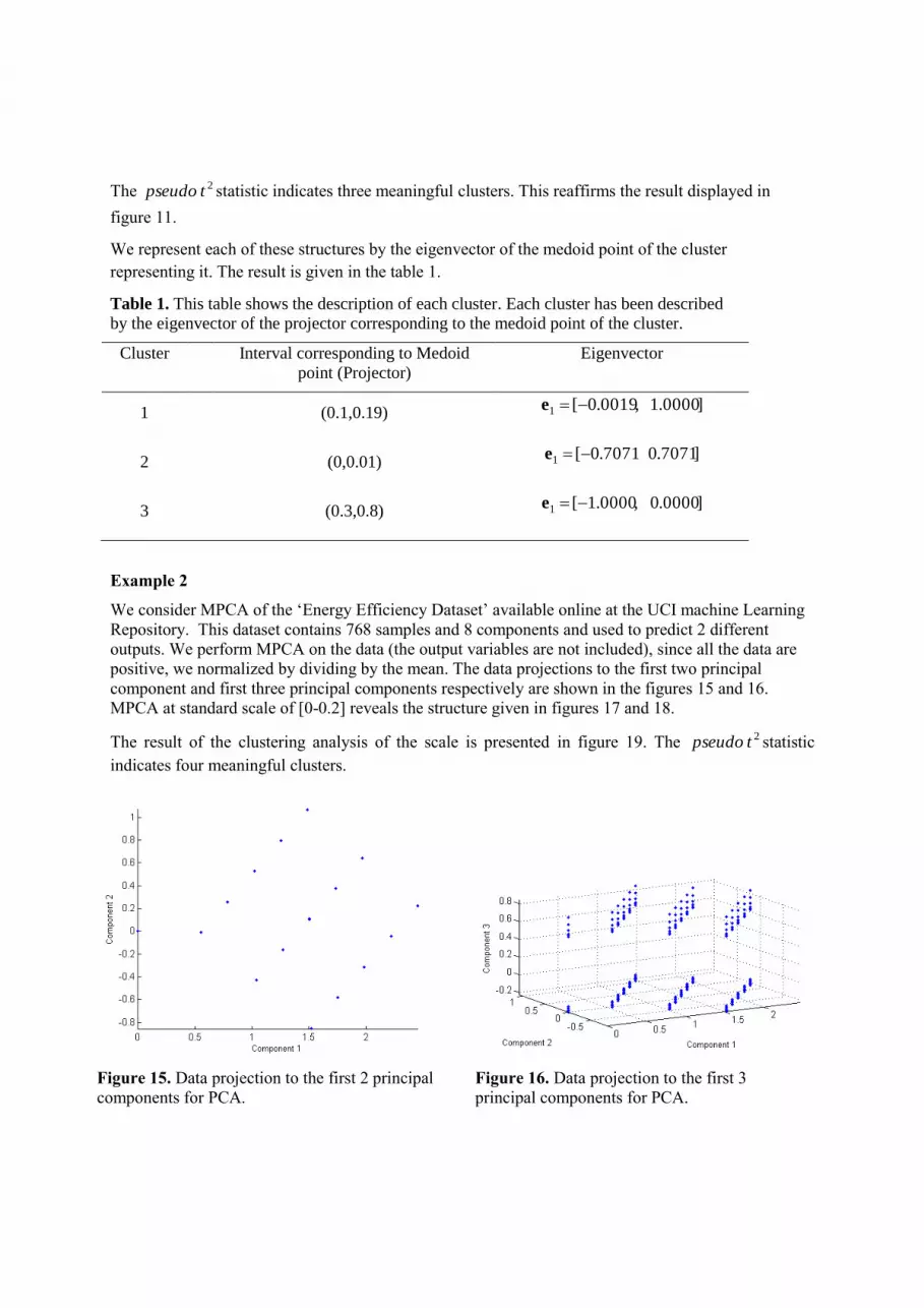
Example 2
We consider MPCA of the ‘Energy Efficiency Dataset’ available online at the UCI machine Learning
Repository. This dataset contains 768 samples and 8 components and used to predict 2 different
outputs. We perform MPCA on the data (the output variables are not included), since all the data are
positive, we normalized by dividing by the mean. The data projections to the first two principal
component and first three principal components respectively are shown in the figures 15 and 16.
MPCA at standard scale of [0-0.2] reveals the structure given in figures 17 and 18.
The result of the clustering analysis of the scale is presented in figure 19. The 2tpseudo statistic
indicates four meaningful clusters.
Figure 15. Data projection to the first 2 principal
components for PCA.
Figure 16. Data projection to the first 3
principal components for PCA.

Figure 17. Data projection to the first 2
principal components using MPCA at standard
scale (0, 0.2).
Figure 18. Data projection to the first 3
principal components using MPCA at standard
scale (0, 0.2)
Figure 19. This diagram shows cluster of
scales on the plane. Scales belonging to the
same cluster are represented by the same
symbol and color. (Color online)
We represent each of these structures by the eigenvector of the medoid point of the cluster
representing it. The result is given in the table 2.
Table 2. This table shows the description of each cluster. Each cluster has been described by the
eigenvectors of the projector corresponding to the medoid point of the cluster.
Cluster Interval corresponding
to Medoid point
Eigenvector
1 (0,0.9) ]6478.0,7618.0,0,0,0,0,0,0[1 e
]7618.0,6478.0,0,0,0,0,0,0[2 e
2 (0,0.2) ]9999.0,0172.0,0,0,0,0,0,0[1 e
]0,0,0000.1,0,0,0,0,0[2 e
3 (0.9-1) ]7190.0,6950.0,0,0,0,0,0,0[1 e
]0,0,0,7355.0,5614.0,0770.0,2587.0,2664.0[2 e
4 0-0.1 ]0,0,0,0762.0,7982.0,4185.0,4266.0[1 e
]0,0,0,0,7979.0,4024.0,2288.0,3860.0[2 e

4.3. Multiscale PCA on Data with Outliers
The presence of outliers in our data serves to obfuscate the underlying structure of the data in PCA.
MPCA is however effective in revealing the underlying structure of data with outliers. By reducing the
upper limit of the scale, we can effectively mitigate the effect of outliers in the analysis of the
principal components without explicit exclusion of these outliers.
Example 3
To test the performance of scaled PCA on data with outliers, data were simulated along known plane
and some outliers were added to this data. This data was embedded into a higher dimensional space
and we seek to recover the original plane from the data by using PCA and MPCA (at various scales).
The angle between the original directional vector and the first principal component of MPCA at
various scales is given in the appendix (see table A1).
We consider a 3-dimensional data sample in which the elements are distributed uniformly on a
plane (2-d) with the directional vectors given as
];0.00000.4472,-0.8944,[u
];0.9129-0.3651,, 0.1826[v
With vector u being the first principal component and few outliers were added as can be seen in figure
19. The projection of the data to the first 2 principal components is shown in figure 20; this has been
influenced by the outliers in the data. MPCA at standard scale of (0-0.8) however gives another
structure which is found to have captured the data quite well as shown in figure 21. The result of the
clustering analysis of the scales is presented in figure 22.
Figure 19. Scatter plot of data in 3-dimension
with a few outlying points.
Figure 20. Data projection to the first 2
principal components using PCA. It can be
observed that the outliers have influenced the
result of the PCA.

Figure 21. Data projection to the first 2 principal
components using MPCA at standard scale of (0,
0.8). The effects of the outliers have been
mitigated.
Figure 22. This diagram shows cluster of scales
on the plane. Scales belonging to the same cluster
are represented by the same symbol and color
(Color online).
We represent each of these structures by the eigenvector of the medoid point of the cluster
representing it. See table 3.
Table 3. This table shows the description of each cluster, described by the eigenvectors of the projector ( 2 )
corresponding to the medoid point of the cluster.
Cluster Interval corresponding to
Medoid point (Projector)
Eigenvector
1 (0.4,1) 0.3704]-0.8579,-,3561.0[1 e
0.2261]-0.4551,,8613.0[2 e
2 (0,0.1) ]0.23490.3382,-0.9113,[1 e
0.8821]0.4679,-0.0538,[2 e
4.4. Criterion for choosing scale for data with outliers
In this section we propose a criterion for deciding an appropriate scale for MPCA in feature extraction
especially for data with outliers.
As mentioned earlier, finding the principal components using definition 3 is equivalent to minimizing
the mean squared distance distortion.
min)],(),([ 2
1,
2
jLiLj
N
ji
i PPdistdist xxxx
Where the dimension k of L is strictly less than the dimension of the data.
Hence we propose that an appropriate scale for a given dimension k could be determined by finding
the ratio of distortion

max,
||)(||
||)()(||
1,
2
1,
2
N
ji
ji
N
ji
jLiL PP
xx
xx
For all ji xx , such that ul ji 2|||| xx
l Is the lower limit of the scale and u is the upper limit.
The ratio of distortion introduced here can also be used in the clustering analysis of scales as a
criterion to determine the PCA structure that describes the cluster.
5. Discussion and Conclusion
5.1. Discussion
For example 3, MPCA at scales ),( ul , 3.00 l , 9.00 u , ul , reveals another structure in the
data that has been obfuscated by the outliers. Table A2 and A3 in the appendix show the results of the
ratio of distortion for 2 different dimensions. This is also consistent with the difference in angle
between the original plane and the principal component computed using MPCA at these scales (see
table A1 in the appendix).
Reducing the upper limit to a very small number may cause MPCA to fit noise while increasing the
lower limit only may cause MPCA to fit outliers if such is present in the data. It is important to note
that by using MPCA, some pairwise distances are exempted in the analysis of principal component
and the percentage of such exempted pairwise distance should be kept to a reasonable number.
As it can be observed in the table A2 and A3 in the appendix, as the lower limit increased, the ratio
of distortion appear to improve (even though the difference in angle is quite large for some scales) but
only because MPCA is fitting outliers. Therefore, in addition to the result of the ratio of distortion, the
percentage of total pairwise distances exempted in the computation of the MPCA at different scales
(especially when 0l ) should be considered in choosing an appropriate scale. A good scale for
MPCA should be one with maximum ratio of distortion and least number of exempted pairwise
distances.
Table A4 in the appendix shows the percentage of pairwise distances of data points exempted in the
computation of MPCA at various scales. It can be concluded that while reducing the upper limit is
good for this data, increasing the lower limit makes MPCA to fit outliers.
5.2. Conclusion
Principal component analysis of high dimension data favour components with high variance. This may
obfuscate hidden geometric structures that may be present in the data. The definition of PCA as the
maximization of the sum of point-to-point squared distances between the orthogonal projections of
data points is a very convenient definition and allows for generalization. In this paper, we introduced
multiscale PCA as maximization of the sum of point-to-point squared distances between the
orthogonal projections of data points for the pairs of points with distances in some intervals (scales).
MPCA is developed to solve the problem of revealing hidden geometric structures in data. The result
of MPCA on data leads to a continuum of PCA structures of the data which is dependent on the
intervals chosen. Analysing the MPCA structures of data reveals some internal structures of the data
especially for data with multiscale structures. To study the MPCA structures of data, we represent the
MPCA structure at a given interval by the cortege of projectors corresponding to MPCA at that
interval; this representation has good and meaningful statistical properties which are discussed. To
reveal underlying geometric structures that may be present in the data, clustering analysis of the PCA
structures at various scales groups together scales with similar PCA structures and separate scales with
dissimilar PCA structures.

For data with clear multiscale structures, the cluster analysis reveals some underlying structures in
the data which conventional PCA cannot reveal due to the fact that such structures are obfuscated by
other structures of higher variance. Each meaningful cluster corresponds to a structure in the data and
we represent each cluster by the medoid point of the cluster and this representative is used to describe
the structure of the data for cluster. We propose the Ratio of Distortion as a criterion for choosing an
appropriate scale for MPCA for feature extraction especially for data with outliers and also as a
criterion for choosing the PCA structure to describe each cluster in the clustering analysis of scales.
Application of MPCA on artificial and real life examples shows that this can be useful. For data with
multi-scale structures, the method was able to reveal some underlying structure in data. The method
was particularly useful in mitigating the influence of outliers on the analysis of principal component
without having to exclude such outliers explicitly.

Appendix
Table A1. The angle between the original component and the result of the first principal
component using MPCA at various scales for the data in example 3. Upper Limit
SCALE 1.0 0.9 0.8 0.7 0.6 0.5 0.4 0.3 0.2 0.1
Lo
wer
Lim
it
0.0 85.2543 6.6465 6.6465 6.6465 6.6465 6.6465 6.6465 6.4516 8.7675 14.918
4
0.1 85.2934 6.5879 6.5879 6.5879 6.5879 6.5879 6.5879 6.3704 8.5396 0.0000
0.2 85.6238 6.1229 6.1229 6.1229 6.1229 6.1229 6.1229 5.6063 0.0000 0.0000
0.3 86.0901 7.2010 7.2010 7.2010 7.2010 7.2010 7.2010 0.0000 0.0000 0.0000
0.4 86.2657 90.0000 90.0000 90.0000 90.0000 90.0000 0.0000 0.0000 0.0000 0.0000
0.5 86.2657 90.0000 90.0000 90.0000 90.0000 0.0000 0.0000 0.0000 0.0000 0.0000
0.6 86.2657 90.0000 90.0000 90.0000 0.0000 0.0000 0.0000 0.0000 0.0000 0.0000
0.7 86.2657 90.0000 90.0000 0.0000 0.0000 0.0000 0.0000 0.0000 0.0000 0.0000
0.8 86.2657 90.0000 0.0000 0.0000 0.0000 0.0000 0.0000 0.0000 0.0000 0.0000
0.9 86.2657 0.0000 0.0000 0.0000 0.0000 0.0000 0.0000 0.0000 0.0000 0.0000
Note: The MPCA at scale 0-1 is the same as PCA. The cell for PCA as being marked with a grey-scale background
Table A2. The ratio of distortion of MPCA at various scales for k = 2. This result is for the
data given in example 3.
Upper Limit
SCALE 1.0 0.9 0.8 0.7 0.6 0.5 0.4 0.3 0.2 0.1
Lo
wer
Lim
it
0.0 0.9030 1.0000 1.0000 1.0000 1.0000 1.0000 1.0000 1.0000 1.0000 1.0000
0.1 0.9196 1.0000 1.0000 1.0000 1.0000 1.0000 1.0000 1.0000 1.0000 0.0000
0.2 0.9734 1.0000 1.0000 1.0000 1.0000 1.0000 1.0000 1.0000 0.0000 0.0000
0.3 0.9906 1.0000 1.0000 1.0000 1.0000 1.0000 1.0000 0.0000 0.0000 0.0000
0.4 0.9971 NaN NaN NaN NaN NaN 0.0000 0.0000 0.0000 0.0000
0.5 0.9971 NaN NaN NaN NaN 0.0000 0.0000 0.0000 0.0000 0.0000
0.6 0.9971 NaN NaN NaN 0.0000 0.0000 0.0000 0.0000 0.0000 0.0000
0.7 0.9971 NaN NaN 0.0000 0.0000 0.0000 0.0000 0.0000 0.0000 0.0000
0.8 0.9971 NaN 0.0000 0.0000 0.0000 0.0000 0.0000 0.0000 0.0000 0.0000
0.9 0.9971 0.0000 0.0000 0.0000 0.0000 0.0000 0.0000 0.0000 0.0000 0.0000
Note: The MPCA at scale 0-1 is the same as PCA. The cell for PCA as being marked with a grey-scale background

Table A3. The ratio of distortion of MPCA at various scales for k = 1. This result is for the
data given in example 3.
Upper Limit
SCALE 1.0 0.9 0.8 0.7 0.6 0.5 0.4 0.3 0.2 0.1
Lo
wer
Lim
it
0.0 0.4695 0.8297 0.8297 0.8297 0.8297 0.8297 0.8297 0.8139 0.7433 0.6748
0.1 0.4989 0.8511 0.8511 0.8511 0.8511 0.8511 0.8511 0.8360 0.7630 0.0000
0.2 0.6467 0.9341 0.9341 0.9341 0.9341 0.9341 0.9341 0.9279 0.0000 0.0000
0.3 0.8679 0.9532 0.9532 0.9532 0.9532 0.9532 0.9532 0.0000 0.0000 0.0000
0.4 0.9851 NaN NaN NaN NaN NaN 0.0000 0.0000 0.0000 0.0000
0.5 0.9851 NaN NaN NaN NaN 0.0000 0.0000 0.0000 0.0000 0.0000
0.6 0.9851 NaN NaN NaN 0.0000 0.0000 0.0000 0.0000 0.0000 0.0000
0.7 0.9851 NaN NaN 0.0000 0.0000 0.0000 0.0000 0.0000 0.0000 0.0000
0.8 0.9851 NaN 0.0000 0.0000 0.0000 0.0000 0.0000 0.0000 0.0000 0.0000
0.9 0.9851 0.0000 0.0000 0.0000 0.0000 0.0000 0.0000 0.0000 0.0000 0.0000
Note: The MPCA at scale 0-1 is the same as PCA. The cell for PCA as being marked with a grey-scale background
Table A4. The percentage of pairwise distances excluded at various scales of MPCA. This
result is for the data given in example 3.
Upper Limit
SCALE 1.0 0.9 0.8 0.7 0.6 0.5 0.4 0.3 0.2 0.1
Lo
wer
Lim
it
0.0 0.00% 11.20% 11.20% 11.20% 11.20% 11.20% 11.20% 15.85% 34.71% 73.53%
0.1 26.47% 37.68% 37.68% 37.68% 37.68% 37.68% 37.68% 42.32% 61.18% 0.00%
0.2 65.29% 76.50% 76.50% 76.50% 76.50% 76.50% 76.50% 81.15% 0.00% 0.00%
0.3 84.15% 95.35% 95.35% 95.35% 95.35% 95.35% 95.35% 0.00% 0.00% 0.00%
0.4 88.80% 100.00% 100.00% 100.00% 100.00% 100.00% 0.00% 0.00% 0.00% 0.00%
0.5 88.80% 100.00% 100.00% 100.00% 100.00% 0.00% 0.00% 0.00% 0.00% 0.00%
0.6 88.80% 100.00% 100.00% 100.00% 0.00% 0.00% 0.00% 0.00% 0.00% 0.00%
0.7 88.80% 100.00% 100.00% 0.00% 0.00% 0.00% 0.00% 0.00% 0.00% 0.00%
0.8 88.80% 100.00% 0.00% 0.00% 0.00% 0.00% 0.00% 0.00% 0.00% 0.00%
0.9 88.80% 0.00% 0.00% 0.00% 0.00% 0.00% 0.00% 0.00% 0.00% 0.00%

References
[1] Jolliffe I T 2002 Principal Component Analysis Second Edition (New York: Springer)
[2] Gorban A N and Zinovyev A Y 2009. Principal Graphs and Manifolds Handbook of Research
on Machine Learning Applications and Trends: Algorithms, Methods and Techniques,.
Information Science Reference.(Preprint arXiv:0809.0490v2)
[3] Zinovyev A 2000 Visualization of Multidimensional Data (In Russian), Krasnoyarsk Technical
State University Press.
[4] Burges C J C 2010 Geometric Methods for Feature Extraction and Dimensional Reduction - A
Guided Tour Data Mining and Knowledge Discovery Handbook (New York: Springer) ed
O Maimon and L Rokach . 2nd Edition ISBN 978-0-387-09822-7 pp 53-82.
[5] Pearson K 1901 On lines and planes of closest fit to systems of points in space. Philosophical
Magazine 2 pp 559-72.
[6] Shlens J 2005. A tutorial on principal component analysis.
http://www.brainmapping.org/NITP/PNA/Readings/pca.pdf (Accessed May 20, 2013)
[7] Arnold R and Jupp P E 2013 Statistics of orthogonal axial frames, Biometrika pp 1-16
(doi: 10.1093/biomet/ast017)
[8] Koren Y and Carmel L 2004 Robust linear dimensionality reduction, Visualization and
Computer Graphics, IEEE Transactions vol.10, no.4, pp.459-70.