improved process monitoring using nonlinear principal component models

Improved Process Monitoring UsingNonlinear Principal Component ModelsDavid Antory,1,† George W. Irwin,2,∗ Uwe Kruger,2,‡ Geoffrey McCullough3,§1Roll-Royce Plc, Controls SCU, PO Box 31, Derby, DE24 8BJ, UK2Intelligent Systems & Control Research Group, School of Electronics &Aerospace Engineering, QUB, Ashby Building, Stranmillis Road, Belfast, BT95AH, UK3Internal Combustion Engines Research Group, School of Mechanical &Aerospace Engineering, QUB, Ashby Building, Stranmillis Road, Belfast, BT95AH, UK

This paper presents two new approaches for use in complete process monitoring. The first concernsthe identification of nonlinear principal component models. This involves the application of linearprincipal component analysis (PCA), prior to the identification of a modified autoassociativeneural network (AAN) as the required nonlinear PCA (NLPCA) model. The benefits are that (i)the number of the reduced set of linear principal components (PCs) is smaller than the number ofrecorded process variables, and (ii) the set of PCs is better conditioned as redundant informationis removed. The result is a new set of input data for a modified neural representation, referred to asa T2T network. The T2T NLPCA model is then used for complete process monitoring, involvingfault detection, identification and isolation.

The second approach introduces a new variable reconstruction algorithm, developed fromthe T2T NLPCA model. Variable reconstruction can enhance the findings of the contributioncharts still widely used in industry by reconstructing the outputs from faulty sensors to producemore accurate fault isolation. These ideas are illustrated using recorded industrial data relatingto developing cracks in an industrial glass melter process. A comparison of linear and nonlinearmodels, together with the combined use of contribution charts and variable reconstruction, ispresented. C© 2008 Wiley Periodicals, Inc.

A preliminary version of this paper entitled “Industrial Process Monitoring Using Nonlin-ear Principal Component Models,” was presented at the 2nd IEEE International Conference onIntelligent Systems, Varna, Bulgaria, June 22–24, 2004.

∗Author to whom all correspondence should be addressed: e-mail: [email protected].†e-mail: [email protected].‡e-mail: [email protected].§e-mail: [email protected].

INTERNATIONAL JOURNAL OF INTELLIGENT SYSTEMS, VOL. 23, 520–544 (2008)C© 2008 Wiley Periodicals, Inc. Published online in Wiley InterScience

(www.interscience.wiley.com). • DOI 10.1002/int.20281

IMPROVED PROCESS MONITORING USING NONLINEAR PCA MODELS 521

1. INTRODUCTION

Modern industrial processes usually involve a large computerized monitoringsystem, where thousands of data values are collected every second. This abundanceof data contains useful information on the process behavior1,2 and is useful forenhancing process efficiency, reliability and safety.3 Statistically based techniquesthat are collectively referred to as multivariate statistical process control (MSPC)have received much attention in this regard.3,4 The multivariate projection methodof MSPC aims to remove the redundancy often observed in the recorded variablesby defining a reduced set of ‘artificial’ or latent variables.5 The variation in therecorded variables is then usually described in terms of these latent variables, withoutsignificant loss of information.

Principal component analysis (PCA) is one of the most popular multivariateprojection methods. It directly analyses the recorded variables without needing priordivision to reflect the input/output structure of the process.6 PCA is a linear steady-state analysis tool. Applying PCA, however, is restricted by the fact that it cannotdescribe nonlinear relationships between the variables. Such behavior often arises,particularly if the process exhibits multiple operating regimes.

To address this, nonlinear extensions to multivariate projection methods havebeen reported, notably by Hastie and Stuetzle7 using principal curves, by Kramer8,9

using autoassociative neural networks (AAN) to implement nonlinear PCA(NLPCA), and by Qin and McAvoy10 using neural networks within the frame-work of partial least squares (PLS). Webb11 and Wilson et al.,12 also proposed anonlinear extension of PCA using radially symmetric kernel functions and radialbasis function (RBF) networks, respectively. In terms of process monitoring, Jiaet al.13 utilized an Input-Training (IT) neural network that was originally proposedby Tan and Mavrouvouniotis.14 An IT network is based on determining a set oflinear principal components (PCs), which is then mapped onto the original plantvariables by a neural network. The number of linear PCs retained is adjusted on thebasis of the accuracy with which the original variable set can be reconstructed. Thefollowing questions arise from the use of an IT network in this context:

(i) What is the geometric meaning of linear PCs in a nonlinear context?(ii) Do linear PCs represent the smallest possible set for representing significant process

variation?(iii) How can the nonlinear relationships between process variables be described?

In this paper, an alternative technique, which exploits the benefits of both AANand IT networks, is presented. This involves the application of PCA, to removelinearly redundant and insignificant information from the recorded process variables,followed by the application of an AAN to these linear PCs, rather than to the processdata. The proposed approach inherits the following benefits from the IT network:fewer variables are used in the AAN, the linear PCs are statistically independent,11

and they are preconditioned, which is favorable for training the AAN. Importantly,the use of an AAN means that the nonlinear PCs can be geometrically interpretedwith respect to the selected network topology, the number of retained nonlinear

International Journal of Intelligent Systems DOI 10.1002/int

522 ANTORY ET AL.

PCs is minimal, and, of course, a nonlinear relationship can be established betweenthe process variables. The new method is thus conceptually superior to using theIT network alone and is computationally less expensive than a conventional AANapplied directly to the original process variables. This modified AAN will be referredto as a T2T network to reflect the identity mapping of the PC scores (see Section 2).

The T2T nonlinear PCA (NLPCA) model is then used for complete conditionmonitoring including fault detection, fault identification, and fault isolation, col-lectively known as fault diagnosis.15 In relation to fault isolation, this paper alsoproposes using a new T2T variable reconstruction algorithm to confirm the findingsof conventional contribution charts.16 For complex industrial processes, relying oncontribution charts alone may not give accurate and reliable fault identification andmay mislead the isolation process. This aspect is illustrated later in an applicationstudy of an industrial glass melter process. Variable reconstruction17,18 is capable ofconfirming the findings of contribution charts. Thus, it produces more reliable faultidentification and strengthens the isolation process.

To demonstrate the utility of these new ideas for fault diagnosis, an industrialapplication study is presented that uses recorded data from an industrial melterprocess. The increased accuracy with which the T2T NLPCA model reconstructsthe process variables leads to a more sensitive monitoring scheme in detecting cracksin the melter compared to the technique proposed by Chen et al.,19 for the sameapplication. This was independently confirmed by ourselves recently.27 Furthermore,when identifying and isolating the source of the faults, it is seen that the contributioncharts only highlight the most significant contributing variables. For a complex fault,such as a developing crack in the melter vessel, this is insufficient since the fault ismanifested in several sensor readings to create a process fault instead of a sensor one.Variable reconstruction enhances the findings by reconstructing the faulty sensors,thus enabling the operator to locate the source of the fault.

The next section gives a brief overview of linear PCA, prior to the descriptionof the AAN in Section 3. The development of the proposed T2T NLPCA modeland T2T variable reconstruction algorithm is presented in Section 4, together with asummary of monitoring statistics and charts for online process monitoring. This isfollowed by the application study to an industrial glass melter process in Section 5.Finally, Section 6 summarizes and concludes this work.

2. LINEAR PCA

For a given data matrix, Z ∈ RK×N , (N � K) in which K observations of N

mean-centered and appropriately scaled process variables are stored as row vectors,the application of PCA gives rise to a reduced set of “artificial” process variables asshown in Figure 1.

T ∈ RK×nL is the score matrix in which K samples of a reduced set of score

variables of dimension nL are stored as column vectors. P ∈ RN×nL is the loading

matrix that represents the contribution of the score variables to the reconstruction (orprediction) of the original process variables, and E ∈ R

K×N is the residual matrix.



Figure 1. Schematic diagram of the PCA decomposition. The original data contains the impor-tant variations for building a model plus noise residuals.

For identifying a PCA model, it is imperative that Z contains reference datadescribing normal process variation. The PCA model is determined by the loadingmatrix, which consists of the n dominant eigenvectors of the covariance matrixSZZ = ZT Z

K−1 ∈ RN×N . For a given observation, z ∈ R

N , the reduced variable set isgiven by

tL = PTz (1)

where tL ∈ RnL is the score vector. The residual vector of this observation, e ∈ R

N ,is then computed as follows:

e = z − PtL = [IN − PPT ]z (2)

where IN is the identity matrix of dimension N . Further information about PCAmay be found in Refs. 6, 20, 21.

3. AUTOASSOCIATIVE NEURAL NETWORKS

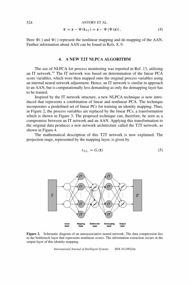
An autoassociative neural network (ANN) is a class of feedforward neuralnetworks that represents a nonlinear identity mapping of a given variable set. Suchnetworks have been proposed as an extension to conventional PCA, where nonlinearscores are represented by the number of nodes in the bottleneck layer as shown inFigure 2.

An AAN consists of mapping, bottleneck and de-mapping layers plus oneinput and one output layer.8 The nodes in the mapping and de-mapping layersusually have sigmoid activation functions, while linear activation functions are usedin the bottleneck and output layers. The input layer takes the measured processvariables (Z) and distributes them to the next layer, while the output layer providesthe prediction of the process variables (Z′).

For a given observation, z, the values of the nonlinear scores variables, tNL ∈R

nNL with nNL being the number of nodes in the bottleneck layer, and the residualvector of the reconstruction �ee, are given by:

tNL = � (z) (3)


524 ANTORY ET AL.

e� = z − � (tNL) = z − � (� (z)) , (4)

Here �(·) and �(·) represent the nonlinear mapping and de-mapping of the AAN.Further information about AAN can be found in Refs. 8, 9.

4. A NEW T2T NLPCA ALGORITHM

The use of NLPCA for process monitoring was reported in Ref. 13, utilizingan IT network.14 The IT network was based on determination of the linear PCAscore variables, which were then mapped onto the original process variables usingan internal neural network adjustment. Hence, an IT network is similar in approachto an AAN, but is computationally less demanding as only the demapping layer hasto be trained.

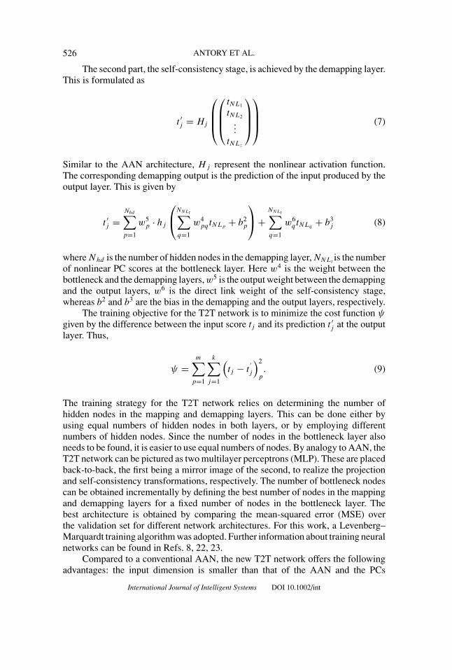
Inspired by the IT network structure, a new NLPCA technique is now intro-duced that represents a combination of linear and nonlinear PCA. The techniqueincorporates a predefined set of linear PCs for training an identity mapping. Thus,in Figure 2, the process variables are replaced by the linear PCs, a transformationwhich is shown in Figure 3. The proposed technique can, therefore, be seen as acompromise between an IT network and an AAN. Applying this transformation tothe original data produces a new network architecture called the T2T network, asshown in Figure 4.

The mathematical description of this T2T network is now explained. Theprojection stage, represented by the mapping layer, is given by

tNLi= Gi(t) (5)

Figure 2. Schematic diagram of an autoassociative neural network. The data compression liesin the bottleneck layer that represents nonlinear scores. The information extraction occurs at theoutput layer of this identity mapping.



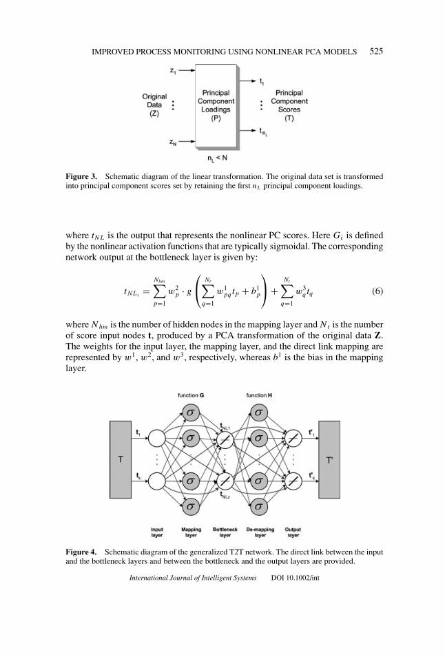
Figure 3. Schematic diagram of the linear transformation. The original data set is transformedinto principal component scores set by retaining the first nL principal component loadings.

where tNL is the output that represents the nonlinear PC scores. Here Gi is definedby the nonlinear activation functions that are typically sigmoidal. The correspondingnetwork output at the bottleneck layer is given by:

tNLi=

Nhm∑p=1

w2p · g

⎛⎝

Nt∑q=1

w1pqtp + b1

p

⎞⎠ +

Nt∑q=1

w3q tq (6)

where Nhm is the number of hidden nodes in the mapping layer and Nt is the numberof score input nodes t, produced by a PCA transformation of the original data Z.The weights for the input layer, the mapping layer, and the direct link mapping arerepresented by w1, w2, and w3, respectively, whereas b1 is the bias in the mappinglayer.

Figure 4. Schematic diagram of the generalized T2T network. The direct link between the inputand the bottleneck layers and between the bottleneck and the output layers are provided.


526 ANTORY ET AL.

The second part, the self-consistency stage, is achieved by the demapping layer.This is formulated as

t ′j = Hj

⎛⎜⎜⎝

⎛⎜⎜⎝

tNL1

tNL2

...tNLz

⎞⎟⎟⎠

⎞⎟⎟⎠ (7)

Similar to the AAN architecture, Hj represent the nonlinear activation function.The corresponding demapping output is the prediction of the input produced by theoutput layer. This is given by

t ′j =Nhd∑p=1

w5p · hj

⎛⎝

NNLt∑q=1

w4pqtNLp

+ b2p

⎞⎠ +

NNLt∑q=1

w6q tNLq

+ b3j (8)

where Nhd is the number of hidden nodes in the demapping layer, NNLtis the number

of nonlinear PC scores at the bottleneck layer. Here w4 is the weight between thebottleneck and the demapping layers, w5 is the output weight between the demappingand the output layers, w6 is the direct link weight of the self-consistency stage,whereas b2 and b3 are the bias in the demapping and the output layers, respectively.

The training objective for the T2T network is to minimize the cost function ψ

given by the difference between the input score tj and its prediction t ′j at the outputlayer. Thus,

ψ =m∑

p=1

k∑j=1

(tj − t

′j

)2

p. (9)

The training strategy for the T2T network relies on determining the number ofhidden nodes in the mapping and demapping layers. This can be done either byusing equal numbers of hidden nodes in both layers, or by employing differentnumbers of hidden nodes. Since the number of nodes in the bottleneck layer alsoneeds to be found, it is easier to use equal numbers of nodes. By analogy to AAN, theT2T network can be pictured as two multilayer perceptrons (MLP). These are placedback-to-back, the first being a mirror image of the second, to realize the projectionand self-consistency transformations, respectively. The number of bottleneck nodescan be obtained incrementally by defining the best number of nodes in the mappingand demapping layers for a fixed number of nodes in the bottleneck layer. Thebest architecture is obtained by comparing the mean-squared error (MSE) overthe validation set for different network architectures. For this work, a Levenberg–Marquardt training algorithm was adopted. Further information about training neuralnetworks can be found in Refs. 8, 22, 23.

Compared to a conventional AAN, the new T2T network offers the followingadvantages: the input dimension is smaller than that of the AAN and the PCs



are preconditioned (statistically independent), which is an advantage for networktraining. The first benefit follows from the number of linear PCs being smallerthan the number of original variables. In addition, the score vectors that representthe linear PCs from the reference data set are mutually orthogonal. Consequently,these represent a preconditioned set of process variables from which insignificantcontributions, such as measurement noise, have been discarded.

The advantages of the proposed T2T NLPCA technique over the IT networkare summarized and elaborated below:

(i) the nonlinear PCs can be geometrically interpreted;(ii) with respect to the selected network topology, the number of retained nonlinear PCs is

minimal; and(iii) the identification of unknown nonlinear scores can be justified.

The geometric interpretation of the proposed technique is as follows: The linearscore variables represent an orthogonal projection of the original process variablesonto the PCA model plane, spanned by the retained loading vectors. This projectionis defined in (1). The T2T network is then used to predict the linear score variablesusing as few nonlinear score variables as possible. In a similar fashion to linearPCA, the T2T network describes a surface, where the mapping layer computes thenonlinear scores variables and the demapping layer calculates the prediction of thelinear score variables. Moreover, this surface is planar for linear PCA, whereas theT2T network describes a nonlinear surface. The dimension of this nonlinear surfaceis given by the number of nonlinear scores retained, i.e., the number of nodes inthe bottleneck layer. Typically, only a few nonlinear scores are necessary for thisidentity mapping.

5. A NEW T2T VARIABLE RECONSTRUCTION ALGORITHM

Linear variable reconstruction (LVR) is based on a subset of recorded processvariables, which have been reconstructed from the rest using an identified PCAmodel.17,18 Fault information in this subset can be removed by such a reconstructionprocess. The new data set will then contain a combination of reconstructed vari-ables and the remaining nonfaulty ones. Using this, condition monitoring (i.e., faultdiagnosis) can be repeated until there is confirmation that abnormal fault signatureshave been successfully removed. This means that the monitored process can rununder normal conditions again. The variable that undergoes reconstruction is theone that contributes most to the fault condition. For sensor faults, this is simplya case of replacing the identified faulty sensor with a reconstructed one to returnthe operation to normal. For a process fault, the interpretation is slightly different.Here reconstruction identifies the sensors affected, although they themselves are notnecessary faulty. This means that an actual sensor may not need to be replaced tobring the process back to normal. Instead, the affected sensors can give a “hint”to the operator as to the fault location. This is illustrated in the application studylater.


528 ANTORY ET AL.

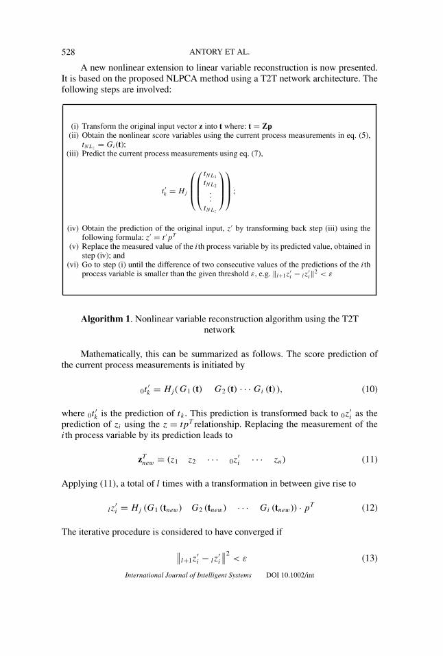
A new nonlinear extension to linear variable reconstruction is now presented.It is based on the proposed NLPCA method using a T2T network architecture. Thefollowing steps are involved:

(i) Transform the original input vector z into t where: t = Zp(ii) Obtain the nonlinear score variables using the current process measurements in eq. (5),

tNLz= Gi(t);

(iii) Predict the current process measurements using eq. (7),

t ′k = Hj

⎛⎜⎜⎝

⎛⎜⎜⎝

tNL1

tNL2

...tNLz

⎞⎟⎟⎠

⎞⎟⎟⎠ ;

(iv) Obtain the prediction of the original input, z′ by transforming back step (iii) using thefollowing formula: z′ = t ′pT

(v) Replace the measured value of the ith process variable by its predicted value, obtained instep (iv); and

(vi) Go to step (i) until the difference of two consecutive values of the predictions of the ithprocess variable is smaller than the given threshold ε, e.g. ‖l+1z

′i − lz

′i‖2 < ε

Algorithm 1. Nonlinear variable reconstruction algorithm using the T2Tnetwork

Mathematically, this can be summarized as follows. The score prediction ofthe current process measurements is initiated by

0t′k = Hj (G1 (t) G2 (t) · · · Gi (t) ), (10)

where 0t′k is the prediction of tk . This prediction is transformed back to 0z

′i as the

prediction of zi using the z = tpT relationship. Replacing the measurement of theith process variable by its prediction leads to

zTnew = (z1 z2 · · · 0z

′i · · · zn) (11)

Applying (11), a total of l times with a transformation in between give rise to

lz′i = Hj (G1 (tnew) G2 (tnew) · · · Gi (tnew)) · pT (12)

The iterative procedure is considered to have converged if

∥∥l+1z

′i − lz

′i

∥∥2< ε (13)



It is straightforward to extend this nonlinear variable reconstruction techniqueto more than one variable.

6. PROCESS MONITORING USING THE T2T NETWORK

Process monitoring can be seen as an integral part of checking a system’s healthto guarantee that it operates normally and without faults. This includes performingfault detection, fault identification, and fault isolation as shown in Figure 5. Theproposed NLPCA technique, built using the T2T network, can be integrated into aprocess-monitoring scheme as follows: The model residuals of the process variablesare used to form a residual-based statistic Q, where

Q = e�T e�. (6)

For this statistic, the 95% and 99% confidence limits are obtained by applying thetheorems developed by Box.24 A Hotelling’s T 2 statistic can also be used to rep-resent the current process variation relative to that incorporated in the referencedata. However, it is important to note that the nonlinear scores may not be normallydistributed and, furthermore, they may not be statistically independent. It is, there-fore, more appropriate to utilize scatter diagrams for which the confidence regionsare obtained based on the kernel density estimation (KDE) of the joint probabilitydensity function (PDF).

A PDF describes the likelihood with which a data point has occurred in theprevious process operation. Nonparametric approaches, like KDE, assume that thedetermination of the density function is carried out by the sum of small kernelfunctions (e.g., Gaussian, triangular or Epanechnikov type25) centered on each datapoint. Examples of the application of the KDE to process monitoring have beenreported in the literature.13,19,26,27

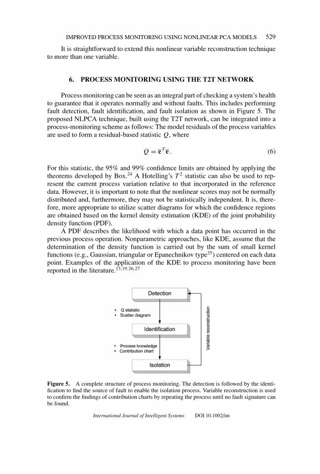
Figure 5. A complete structure of process monitoring. The detection is followed by the identi-fication to find the source of fault to enable the isolation process. Variable reconstruction is usedto confirm the findings of contribution charts by repeating the process until no fault signature canbe found.


530 ANTORY ET AL.

During monitoring, when the process exhibits an “out-of-statistical-control”behavior, it is important to determine the root cause of this.6 In relation to conven-tional MSPC, Miller et al.16 proposed the use of contribution charts for finding thevariable contributions to univariate statistics. In this work, the variable contributionsto the Q statistic were used to diagnose anomalous process behavior. Unfortunately,contribution charts only highlight variables which give the most significant contri-bution to the fault. Relying on contribution charts alone may thus not give accurateand reliable information to the operator on which to take action. Variable reconstruc-tion provides a mechanism to complement the findings of the contribution chartsto identify and isolate the fault source correctly. Reconstruction is performed usingthe remaining nonfaulty sensors to reconstruct the faulty one. Reconstruction is aniterative process which repeats continuously until a certain threshold is reached.Normally, the residual is used as the threshold value. When the new residual fallsbelow the threshold value ε, the reconstruction is terminated.

7. A CRACK DETECTION IN AN INDUSTRIAL

GLASS MELTER PROCESS

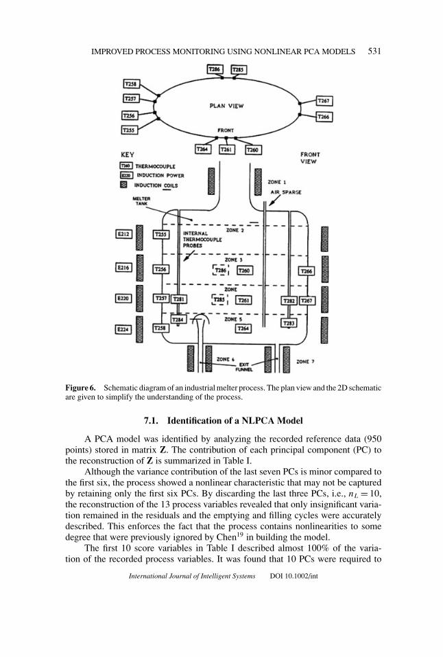
A melter process28 is part of the disposal procedure of a highly radioactivesubstance. The waste material is preprocessed by an evaporation treatment and ahighly radioactive powder remains. This powder is then clad in a glass layer duringthe melter process. The melter consists of a vessel, two exit funnels through whichthe melted load flows out, and several induction coils. The vessel is continuouslyfilled with the radioactive powder, and raw glass is discretely introduced in the formof glass frit. This binary composition is heated by four induction coils, which arepositioned around the vessel. Because of the heating procedure, the glass is meltedhomogeneously. The process of filling and heating continues until the desired heightof the liquid column is reached. The molten mixture is then poured out through oneof the exit funnels. After the content of the vessel has been emptied to the height ofthe nozzle, the next cycle of filling and heating begins. This process is illustrated inFigure 6.

Measurements of eight temperatures, the power in four induction coils, anda voltage were taken every 5 min. The filling and emptying cycles resulted in anonlinear relationship between the temperatures, power in the induction coils, andvoltage. The melter vessel is made of graphite, which is a brittle material. As aresult of the strong temperature variations to which the vessel is frequently exposed,cracks along the regions of high-thermal stress may occur. These cracks not onlydamage the shell of the melter but may also allow radioactive material to escape. Itis, therefore, necessary to detect such cracks at the earliest possible opportunity.

A data set from the melter process was available, which included normal processvariation over a period of about 85 h and an abnormal process situation, resultingfrom a developing crack. This data set contained 13 variables and 1050 samples at asampling frequency of 5 min. The last 100 points correspond to a developing crackin the melter vessel.



Figure 6. Schematic diagram of an industrial melter process. The plan view and the 2D schematicare given to simplify the understanding of the process.

7.1. Identification of a NLPCA Model

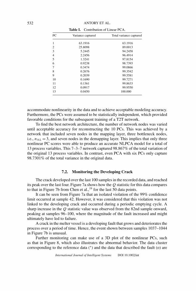
A PCA model was identified by analyzing the recorded reference data (950points) stored in matrix Z. The contribution of each principal component (PC) tothe reconstruction of Z is summarized in Table I.

Although the variance contribution of the last seven PCs is minor compared tothe first six, the process showed a nonlinear characteristic that may not be capturedby retaining only the first six PCs. By discarding the last three PCs, i.e., nL = 10,the reconstruction of the 13 process variables revealed that only insignificant varia-tion remained in the residuals and the emptying and filling cycles were accuratelydescribed. This enforces the fact that the process contains nonlinearities to somedegree that were previously ignored by Chen19 in building the model.

The first 10 score variables in Table I described almost 100% of the varia-tion of the recorded process variables. It was found that 10 PCs were required to


532 ANTORY ET AL.

Table I. Contribution of Linear PCA.

PC Variance captured Total variance captured

1 63.1916 63.19162 25.8098 89.00133 5.2445 94.24584 2.2456 96.49145 1.3241 97.81546 0.9238 98.73937 0.3474 99.08668 0.2676 99.35429 0.2039 99.558110 0.1690 99.727111 0.1361 99.863312 0.0917 99.955013 0.0450 100.000

accommodate nonlinearity in the data and to achieve acceptable modeling accuracy.Furthermore, the PCs were assumed to be statistically independent, which providedfavorable conditions for the subsequent training of a T2T network.

To find the best network architecture, the number of network nodes was varieduntil acceptable accuracy for reconstructing the 10 PCs. This was achieved by anetwork that included seven nodes in the mapping layer, three bottleneck nodes,i.e., nNL = 3, and seven nodes in the demapping layer. This implies that only threenonlinear PC scores were able to produce an accurate NLPCA model for a total of13 process variables. This 7–3–7 network captured 98.867% of the total variation ofthe original 13 process variables. In contrast, even PCA with six PCs only capture98.7301% of the total variance in the original data.

7.2. Monitoring the Developing Crack

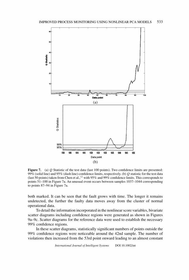
The crack developed over the last 100 samples in the recorded data, and reachedits peak over the last four. Figure 7a shows how the Q statistic for this data comparesto that in Figure 7b from Chen et al.,19 for the last 50 data points.

It can be seen from Figure 7a that an isolated violation of the 99% confidencelimit occurred at sample 42. However, it was considered that this violation was notlinked to the developing crack and occurred during a periodic emptying cycle. Asharp increase in the Q statistic value was observed from the 82nd sample onward,peaking at samples 96–100, where the magnitude of the fault increased and mightultimately have led to failure.

A crack in the melter vessel is a developing fault that grows and deteriorates theprocess over a period of time. Hence, the event shown between samples 1037–1044in Figure 7b is unusual.

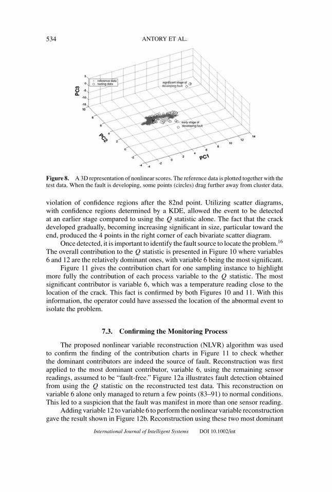
Further monitoring can make use of a 3D plot of the nonlinear PCs, suchas that in Figure 8, which also illustrates the abnormal behavior. The data clustercorresponding to the reference data (∗) and the data that described the fault (o) are



(a)

(b)

Figure 7. (a) Q Statistic of the test data (last 100 points). Two confidence limits are presented:99% (solid line) and 95% (dash line) confidence limits, respectively. (b) Q statistic for the test data(last 50 points) taken from Chen et al.,12 with 95% and 99% confidence limits. This corresponds topoints 51–100 in Figure 7a. An unusual event occurs between samples 1037–1044 correspondingto points 87–94 in Figure 7a.

both marked. It can be seen that the fault grows with time. The longer it remainsundetected, the further the faulty data moves away from the cluster of normaloperational data.

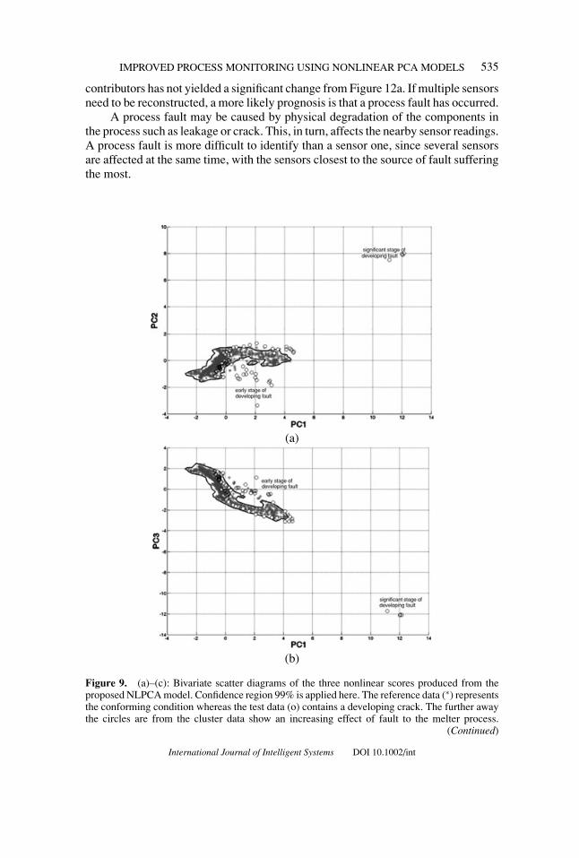
To detail the information incorporated in the nonlinear score variables, bivariatescatter diagrams including confidence regions were generated as shown in Figures9a–9c. Scatter diagrams for the reference data were used to establish the necessary99% confidence regions.

In these scatter diagrams, statistically significant numbers of points outside the99% confidence regions were noticeable around the 42nd sample. The number ofviolations then increased from the 53rd point onward leading to an almost constant


534 ANTORY ET AL.

Figure 8. A 3D representation of nonlinear scores. The reference data is plotted together with thetest data. When the fault is developing, some points (circles) drag further away from cluster data.

violation of confidence regions after the 82nd point. Utilizing scatter diagrams,with confidence regions determined by a KDE, allowed the event to be detectedat an earlier stage compared to using the Q statistic alone. The fact that the crackdeveloped gradually, becoming increasing significant in size, particular toward theend, produced the 4 points in the right corner of each bivariate scatter diagram.

Once detected, it is important to identify the fault source to locate the problem.16

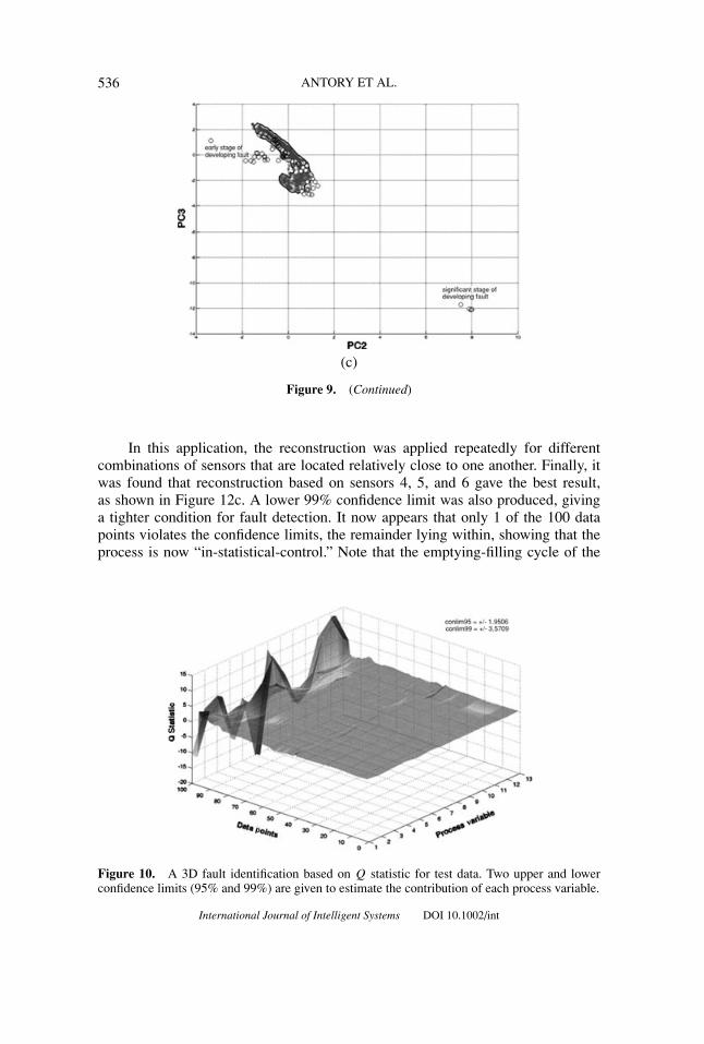
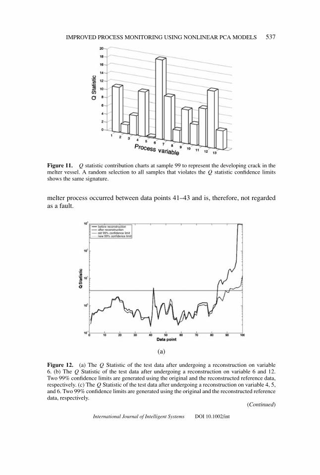
The overall contribution to the Q statistic is presented in Figure 10 where variables6 and 12 are the relatively dominant ones, with variable 6 being the most significant.

Figure 11 gives the contribution chart for one sampling instance to highlightmore fully the contribution of each process variable to the Q statistic. The mostsignificant contributor is variable 6, which was a temperature reading close to thelocation of the crack. This fact is confirmed by both Figures 10 and 11. With thisinformation, the operator could have assessed the location of the abnormal event toisolate the problem.

7.3. Confirming the Monitoring Process

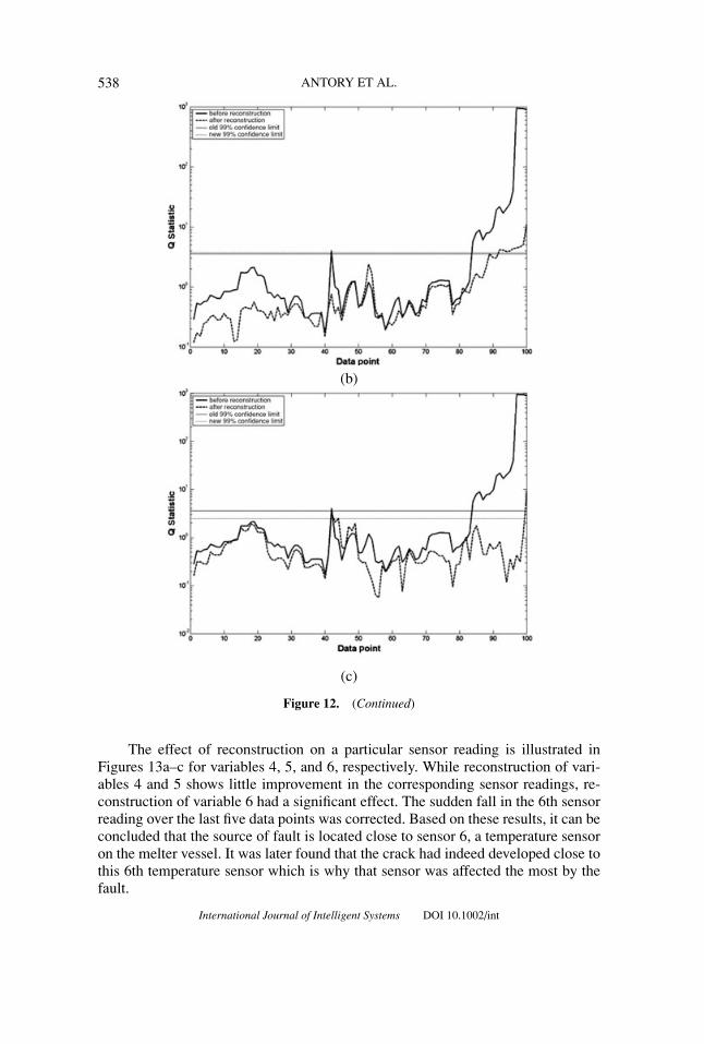
The proposed nonlinear variable reconstruction (NLVR) algorithm was usedto confirm the finding of the contribution charts in Figure 11 to check whetherthe dominant contributors are indeed the source of fault. Reconstruction was firstapplied to the most dominant contributor, variable 6, using the remaining sensorreadings, assumed to be “fault-free.” Figure 12a illustrates fault detection obtainedfrom using the Q statistic on the reconstructed test data. This reconstruction onvariable 6 alone only managed to return a few points (83–91) to normal conditions.This led to a suspicion that the fault was manifest in more than one sensor reading.

Adding variable 12 to variable 6 to perform the nonlinear variable reconstructiongave the result shown in Figure 12b. Reconstruction using these two most dominant



contributors has not yielded a significant change from Figure 12a. If multiple sensorsneed to be reconstructed, a more likely prognosis is that a process fault has occurred.

A process fault may be caused by physical degradation of the components inthe process such as leakage or crack. This, in turn, affects the nearby sensor readings.A process fault is more difficult to identify than a sensor one, since several sensorsare affected at the same time, with the sensors closest to the source of fault sufferingthe most.

(a)

(b)

Figure 9. (a)–(c): Bivariate scatter diagrams of the three nonlinear scores produced from theproposed NLPCA model. Confidence region 99% is applied here. The reference data (∗) representsthe conforming condition whereas the test data (o) contains a developing crack. The further awaythe circles are from the cluster data show an increasing effect of fault to the melter process.

(Continued)


536 ANTORY ET AL.

(c)

Figure 9. (Continued)

In this application, the reconstruction was applied repeatedly for differentcombinations of sensors that are located relatively close to one another. Finally, itwas found that reconstruction based on sensors 4, 5, and 6 gave the best result,as shown in Figure 12c. A lower 99% confidence limit was also produced, givinga tighter condition for fault detection. It now appears that only 1 of the 100 datapoints violates the confidence limits, the remainder lying within, showing that theprocess is now “in-statistical-control.” Note that the emptying-filling cycle of the

Figure 10. A 3D fault identification based on Q statistic for test data. Two upper and lowerconfidence limits (95% and 99%) are given to estimate the contribution of each process variable.



Figure 11. Q statistic contribution charts at sample 99 to represent the developing crack in themelter vessel. A random selection to all samples that violates the Q statistic confidence limitsshows the same signature.

melter process occurred between data points 41–43 and is, therefore, not regardedas a fault.

(a)

Figure 12. (a) The Q Statistic of the test data after undergoing a reconstruction on variable6. (b) The Q Statistic of the test data after undergoing a reconstruction on variable 6 and 12.Two 99% confidence limits are generated using the original and the reconstructed reference data,respectively. (c) The Q Statistic of the test data after undergoing a reconstruction on variable 4, 5,and 6. Two 99% confidence limits are generated using the original and the reconstructed referencedata, respectively.

(Continued)


538 ANTORY ET AL.

(b)

(c)


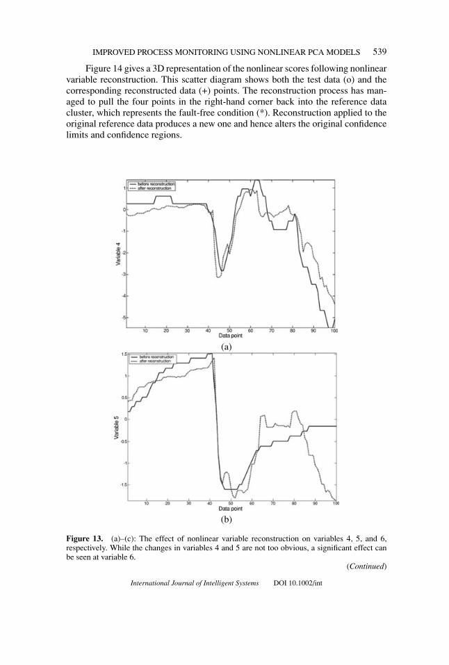
The effect of reconstruction on a particular sensor reading is illustrated inFigures 13a–c for variables 4, 5, and 6, respectively. While reconstruction of vari-ables 4 and 5 shows little improvement in the corresponding sensor readings, re-construction of variable 6 had a significant effect. The sudden fall in the 6th sensorreading over the last five data points was corrected. Based on these results, it can beconcluded that the source of fault is located close to sensor 6, a temperature sensoron the melter vessel. It was later found that the crack had indeed developed close tothis 6th temperature sensor which is why that sensor was affected the most by thefault.



Figure 14 gives a 3D representation of the nonlinear scores following nonlinearvariable reconstruction. This scatter diagram shows both the test data (o) and thecorresponding reconstructed data (+) points. The reconstruction process has man-aged to pull the four points in the right-hand corner back into the reference datacluster, which represents the fault-free condition (*). Reconstruction applied to theoriginal reference data produces a new one and hence alters the original confidencelimits and confidence regions.

(a)

(b)

Figure 13. (a)–(c): The effect of nonlinear variable reconstruction on variables 4, 5, and 6,respectively. While the changes in variables 4 and 5 are not too obvious, a significant effect canbe seen at variable 6.

(Continued)


540 ANTORY ET AL.

(c)


Using scatter diagrams, the process variation encapsulated in the nonlinearscore variables can be shown.27 The confidence regions of the scatter diagrams wereidentified using kernel density estimation (KDE) similar to those in Figures 9a–c.However, this time the new confidence regions were created using the reconstructedreference data. The use of scatter diagrams was motivated by the fact that thenonlinear score variables may not be normally distributed and, consequently, theassumption imposed on the Hotelling’s T 2 statistic may be violated.

Figure 14. 3D representation of nonlinear scores after reconstruction on variable 4, 5, and 6.



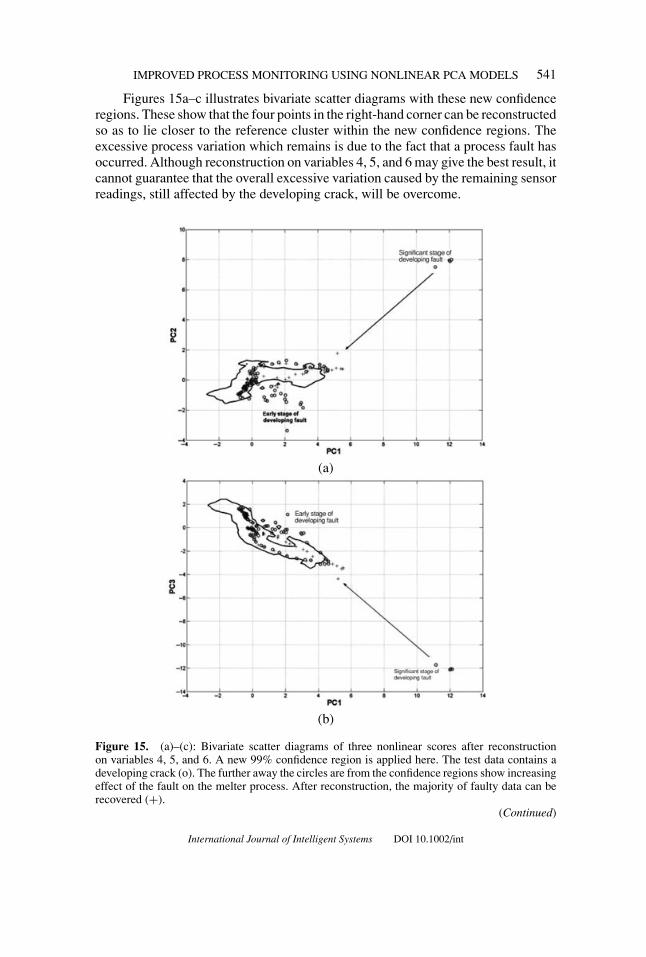
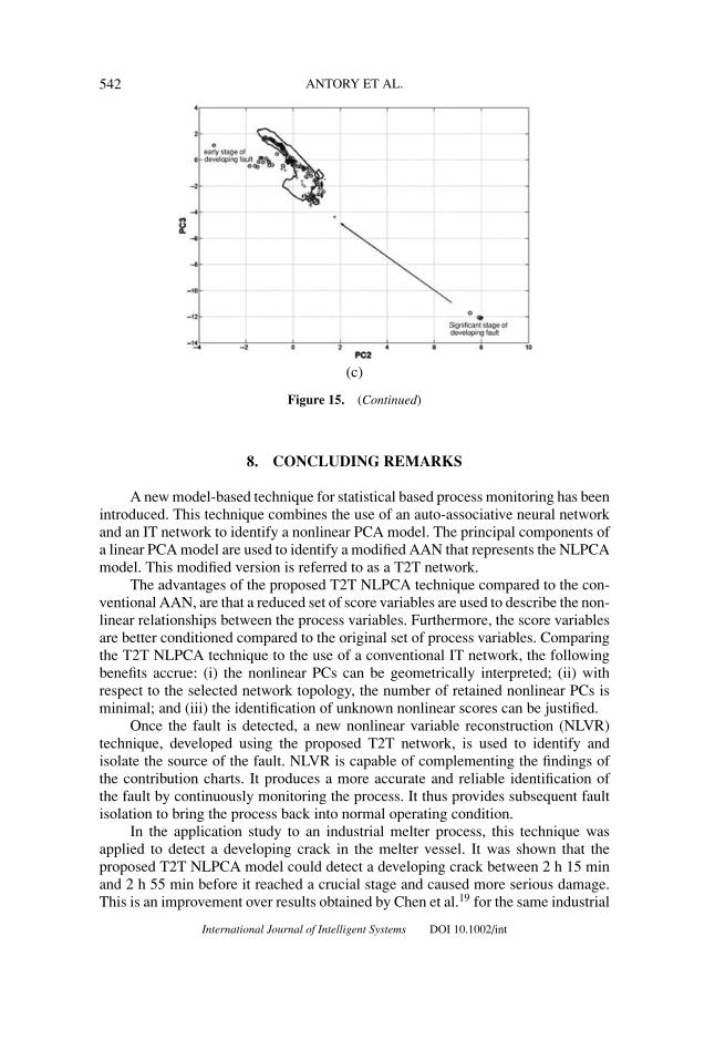
Figures 15a–c illustrates bivariate scatter diagrams with these new confidenceregions. These show that the four points in the right-hand corner can be reconstructedso as to lie closer to the reference cluster within the new confidence regions. Theexcessive process variation which remains is due to the fact that a process fault hasoccurred. Although reconstruction on variables 4, 5, and 6 may give the best result, itcannot guarantee that the overall excessive variation caused by the remaining sensorreadings, still affected by the developing crack, will be overcome.

(a)

(b)

Figure 15. (a)–(c): Bivariate scatter diagrams of three nonlinear scores after reconstructionon variables 4, 5, and 6. A new 99% confidence region is applied here. The test data contains adeveloping crack (o). The further away the circles are from the confidence regions show increasingeffect of the fault on the melter process. After reconstruction, the majority of faulty data can berecovered (+).

(Continued)


542 ANTORY ET AL.

(c)


8. CONCLUDING REMARKS

A new model-based technique for statistical based process monitoring has beenintroduced. This technique combines the use of an auto-associative neural networkand an IT network to identify a nonlinear PCA model. The principal components ofa linear PCA model are used to identify a modified AAN that represents the NLPCAmodel. This modified version is referred to as a T2T network.

The advantages of the proposed T2T NLPCA technique compared to the con-ventional AAN, are that a reduced set of score variables are used to describe the non-linear relationships between the process variables. Furthermore, the score variablesare better conditioned compared to the original set of process variables. Comparingthe T2T NLPCA technique to the use of a conventional IT network, the followingbenefits accrue: (i) the nonlinear PCs can be geometrically interpreted; (ii) withrespect to the selected network topology, the number of retained nonlinear PCs isminimal; and (iii) the identification of unknown nonlinear scores can be justified.

Once the fault is detected, a new nonlinear variable reconstruction (NLVR)technique, developed using the proposed T2T network, is used to identify andisolate the source of the fault. NLVR is capable of complementing the findings ofthe contribution charts. It produces a more accurate and reliable identification ofthe fault by continuously monitoring the process. It thus provides subsequent faultisolation to bring the process back into normal operating condition.

In the application study to an industrial melter process, this technique wasapplied to detect a developing crack in the melter vessel. It was shown that theproposed T2T NLPCA model could detect a developing crack between 2 h 15 minand 2 h 55 min before it reached a crucial stage and caused more serious damage.This is an improvement over results obtained by Chen et al.19 for the same industrial



melter process data. The NLVR algorithm also provides an important means foridentifying and isolating the source of process fault: the developing cracks in themelter vessel in the vicinity of temperature sensor 6th in this case.

Acknowledgment

David Antory wishes to acknowledge the financial support of the Virtual EngineeringCentre, Queen’s University Belfast (www.vec.qub.ac.uk), Belfast, BT9 5AH, Northern Ireland,United Kingdom.

References

1. Piovoso MJ. Process data chemometrics. IEEE Trans Instrum Meas 1992;41(2):262–268.2. MacGregor JF. Using on-line process data to improve quality: challenges for statisticians.

Int Stat Rev 1997:65(3):309–323.3. MacGregor JF, Kourti T. Statistical process control of multivariate processes. Control Eng

Practice 1995;3(3):403–414.4. Kruger U, Chen Q, Sandoz DJ, McFarlane RC. Extended PLS approach for enhanced

condition monitoring of industrial processes. AIChE J 2001;47(9):2076–2091.5. Wise BM, Gallagher NB. The process chemometrics approach to process monitoring and

fault detection. J Process Control 1996;6(6):329–348.6. Jackson JE. A user’s guide to principal components. New York: Wiley; 1991.7. Hastie T, Stuetzle W. Principal curves. J Am Stat Asso 1989:84(406):502–517.8. Kramer MA. Auto-associative neural networks. Comput Chem Eng 1992;16(4):313–328.9. Kramer MA. Nonlinear principal component analysis using auto-associative neural net-

works. AIChE J 1991:37(4):313–328.10. Qin SJ, McAvoy TJ. Nonlinear PLS modeling using neural networks. Comput Chem Eng

1992;16(4):379–391.11. Webb AR. An approach to non-linear principal components analysis using radially symmet-

ric kernel functions. Stat Comput 1996:6:159–168.12. Wilson DJH, Irwin GW, Lightbody G. RBF principal manifolds for process monitoring.

IEEE Trans Neural Netw 1999:10(6):1424–1434.13. Jia F, Martin EB, Morris AJ. Non-linear principal component analysis with applications to

process fault detection. Comput Chem Eng 1998:22: S851–S854.14. Tan S, Mavrovouniotis ML. Reducing data dimensionality through optimizing neural net-

work inputs. AIChE J 1995:41(6):1471–1480.15. Russell EL, Chiang LH, Braatz RD. Data-driven techniques for fault detection and diagnosis

in chemical processes. London: Springer-Verlag; 2000.16. Miller P, Swanson RE, Heckler CE. Contribution plots: A missing link in multivariate quality

control. Appl Math Comp Sci 1998:8 (4):775–792.17. Dunia R, Qin SJ, Edgar TF, McAvoy TJ. Identification of faulty sensors using principal

component analysis. J Process Syst Eng 1996:10(10):2797–2812.18. Dunia R, Qin SJ. Joint diagnosis of process and sensor faults using principal component

analysis. Control Eng Practice 1998:6:457–469.19. Chen Q, Wynne RJ, Goulding P, Sandoz D. The application of principal component anal-

ysis and kernel density estimation to enhance process monitoring. Control Eng Practice2000:8:531–543.

20. Jolliffe IT. Principal component analysis. New York: Springer-Verlag; 1985.21. Jackson JE. Principal components and factor analysis: part i – principal components. J

Quality Technol 1980:12(4):201–213.22. Smith M. Neural networks for statistical modeling. New York: Van Nostrand Reinhold;

1993.


544 ANTORY ET AL.

23. Nørgaard M, Ravn O, Poulsen NK, Hansen LK. Neural networks for modeling and controlof dynamic systems. London: Springer-Verlag; 2000.

24. Box GEP. Some theorems on quadratic forms applied in the study of analysis of varianceproblems. Ann Math Stat 1954:25(2):290–302.

25. Silverman BW. Density estimation. London: Chapman & Hall; 1986.26. Martin EB, Morris AJ. Non-parametric confidence bounds for process performance moni-

toring charts. J Process Control 1996:6(6):349–358.27. Antory D, Kruger U, Irwin GW, McCullough G. Industrial process monitoring using nonlin-

ear principal component models. In: Proc 2nd IEEE Int Conf on Intelligent Systems, Varna,Bulgaria; June 2004. Vol 1, pp 293–298,

28. Kruger U. Multivariate statistical monitoring for improved control of complex industrialprocesses. EngD Thesis, Faculty of Science and Engineering, University of Manchester,UK; 2001.


improved process monitoring using nonlinear principal component models

Documents