guaranteed quality tetrahedral delaunay meshing for medical images
TRANSCRIPT
Guaranteed Quality Tetrahedral Delaunay Meshing for
Medical Images
Panagiotis A. Foteinosa,b,∗, Andrey N. Chernikovb, Nikos P. Chrisochoidesb
aDepartment of Computer Science, College of William & Mary, Williamsburg, 23185,Virginia, USA
bDepartment of Computer Science, Old Dominion University, Norfolk, 23569, Virginia,USA
Abstract
In this paper, we present a Delaunay refinement algorithm for meshing 3Dmedical images. Given that the surface of the represented object is a smooth2-manifold without boundary, we prove that (a) all the tetrahedra of the
output mesh have radius-edge ratio less than√√
3 + 2 (≈ 1.93), (b) all theboundary facets have planar angles larger than 30 degrees, (c) the symmetric(2-sided) Hausdorff distance between the object surface and mesh bound-ary is bounded from above by a user-specified parameter, and (d) the meshboundary is ambient isotopic to the object surface. The first two guaranteesassure that our algorithm produces elements of bounded radius-edge ratio.The last two guarantees assure that the mesh boundary is a good geometricand topological approximation of the object surface. Our method also offerscontrol over the size of tetrahedra in the final mesh. Experimental evaluationof our algorithm on synthetic and real medical data illustrates the theory andshows the effectiveness of our method.
Keywords: Delaunay mesh generation; medical images; quality; fidelity;
1. Introduction
Delaunay meshing is a popular technique for generating tetrahedral meshes,since it is able to mesh various domains such as: polyhedral domains [1, 2],
∗Corresponding authorEmail addresses: [email protected] (Panagiotis A. Foteinos), [email protected]
(Andrey N. Chernikov), [email protected] (Nikos P. Chrisochoides)
Preprint submitted to Elsevier November 16, 2013

domains bounded by surfaces [3, 4], or multi-labeled images [5, 6], offeringat the same time mathematical guarantees on the quality and the fidelity ofthe final mesh.
In the literature, Delaunay refinement techniques have been employed tomesh objects whose surface is already meshed as a Piecewise Linear Complex(PLC) [1, 2, 7–9]. The challenge in this category of techniques is that thequality of the input PLC affects the quality of the final volume mesh. Forexample, if the input angles of the PLC are small, then even terminationmight be compromised [10]. For images, one way to alleviate this challengeis to consider the faces of each outer voxel as the input PLC, since thesefaces meet at large angles (90 or 180). However, this would result in anunnecessarily large final mesh.
Another approach is to assume that the object Ω to be meshed is knownonly through an implicit function f : R3 → Z such that points in differ-ent regions of interest evaluate f differently. This assumption covers a widerange of inputs used in modeling and simulation, such as parametric sur-faces/volumes [3], level-sets, and segmented multi-labeled images [5, 6, 11],the focus of this paper. If the subsequent simulation permits sharp featuresof the domain to be rounded-off, such functions can be used to representPLCs as well [11], a fact that renders this approach quite general. It shouldbe noted that these methods do not suffer from any small input angle arti-facts introduced by the initial conversion to PLCs, since the isosurface ∂Ωof the object Ω is recovered and meshed during refinement. In this paper,we deal with objects whose surface is a smooth 2-manifold (see Section 2).It is the algorithm’s responsibility to mesh both the surface and the interiorof the object such that the mesh boundary describes the object surface in away that meets the predefined fidelity and quality requirements.
The quality of an element is traditionally measured in terms of its circum-radius-to-shortest-edge ratio or radius-edge ratio for short. It is desirablethat the mesh elements have radius-edge ratio bounded from above. Meshessatisfying that bounded ratio property are called almost-good meshes in theliterature [12]. Miller et al. [13] show that almost-good meshes guaranteeoptimal convergence rates for approximate solutions of Poisson’s equation.
Delaunay volume meshing algorithms extend the popular Delaunay sur-face meshing and reconstruction algorithms described in [14, 15], and theyoffer quality and fidelity guarantees [3, 4] under the assumption that the sur-face of the object is smooth [3, 15] or does not form input angles less than90 [4]. However, the quality achieved by these algorithms is somewhat weak:
2

the upper bound for the elements’ radius-edge ratio is larger than 4. In con-
trast, the upper bound guaranteed by our algorithm is√√
3 + 2 (≈ 1.93). Toour knowledge, our algorithm is the first volume Delaunay mesher for surfacesachieving such a small radius-edge ratio with these fidelity guarantees.
Almost-good meshes, however, might contain nearly flat elements, the socalled slivers. The reason is that slivers can have a very small radius-edgeratio and at the same time a very small dihedral angle. In the literature,there are post-processing techniques that given an almost-good mesh, theyare able to remove slivers. See for example the work of Li and Teng [12],the exudation technique of Cheng et al. [8], and the sliver perturbation ofTournois et al. [16]. In fact, the sliver removal technique of Li and Teng [12]requires a low radius-edge ratio, since the lower the radius-edge ratio, thelarger the guaranteed bound on the minimum dihedral angles. This is anothermotivation for achieving low radius-edge ratio.
The success of Delaunay techniques to approximate the surface relies onthe notion of ε-samples, first introduced by Amenta and Bern [17]. The con-struction of ε-samples directly from the surface is a challenging task. In theliterature, however, it is assumed that either such a sample is known [15,17, 18] or that an initial sparse sample is given on every connected compo-nent [3, 4, 19]. In this paper, we propose a method that starts directly fromlabeled images and computes the appropriate sample on the fly.
In summary, we present a Delaunay refinement algorithm which:
• operates directly on images, samples and meshes the surface and thevolume of the represented biological object at the same time,
• is proved to generate tetrahedra with radius-edge ratio less than√√3 + 2 (≈ 1.93) and boundary facets with planar angles more than
30,
• is proved to yield meshes of good fidelity, i.e., the mesh surface isguaranteed to be a faithful geometric and topological approximation ofthe object’s surface, and
• offers control over the size and the grading of the final mesh.
In the literature, there are also non-Delaunay surface and volume meshingalgorithms for 3D images. Marching Cubes [20] is a very popular techniquefor surface meshing; it guarantees, however, neither good quality triangu-lar facets nor faithful surface approximation. Furthermore, since the cubes
3

have a very small size (close to the voxel size), Marching Cubes does notoffer a way to control the size of the mesh. Molino et al. [21] develop theRed-Green Mesh (RGM) method. RGM starts by meshing an initial body-centric cubic (BCC) lattice which is then compressed such that its boundaryfit on the surface. RGM gives, however, no quality or surface approxima-tion guarantees. Another lattice-based method is the Isosurface Stuffing ofLabelle and Shewchuk [11]. They prove that the graded version of the finalmesh consists of elements with dihedral angles larger than 1.66. The LatticeDecimation method proposed by Chernikov and Chrisochoides [22] is guar-anteed to produce a good geometric approximation of the underlying object;however, topological faithfulness is not guaranteed. Alliez et al. [23] intro-duce a Delaunay-based optimization technique. Specifically, they iterativelycompute the new locations of the points by minimizing a quadratic energy.The connectivity of these points is recalculated by finding their Delaunay tri-angulation each time. They show that this technique produces meshes thatrespect the boundary of the domain. Klingner and Shewchuk [24] extend thework of Freitag and Ollivier-Gooch [25] by proposing smoothing and topo-logical transformations which improve the quality of the mesh substantially.The execution time, however, can be very high, even for small mesh sizeproblems.
The rest of this paper is organized as follows: Section 2 provides thenecessary definitions and Section 3 outlines our algorithm. Section 4 provesthe quality, Section 5 proves the good grading, and Section 6 proves thefidelity guarantees. Finally, Section 7 elaborates on certain implementationdetails, Section 8 assesses the practical value of our work on both syntheticand real medical data, and Section 9 concludes our paper.
2. Preliminaries
Let I ⊂ R3 be the (spatial) domain of a multi-tissue segmented image.I is the input of our algorithm that contains the object Ω ⊂ I to be meshed.We assume that the object is partitioned into a finite number of n distinct
tissues Ω =n⋃i
Ωi, i = 1, . . . , n. Each Ωi defines an interface ∂Ωi that consists
of the set of points that lie on the boundary between Ωi and at least one moretissue or the background of the image. The isosurface ∂Ω of Ω is then the
collection of all interfaces; that is, ∂Ω =n⋃i
∂Ωi, i = 1, . . . , n. We assume
4

that we are given a function f : I → −1, 0, 1, . . . , n, which classifies everypoint p ∈ I appropriately. Specifically, p evaluates f to −1 if it lies on ∂Ω,to 0 if it lies in the background (i.e., outside the object), or to a positiveinteger i if it belongs to the tissue Ωi. The existence of such a function isa quite reasonable assumption: f can be constructed or approximated fromthe image voxels quite well for any segmented image (see Section 7 for detailson f ’s implementation).
As is generally the case in the literature [3, 15, 19], we also assume that∂Ω is a smooth (twice differentiable) 2-manifold without boundary.
Definition 1 (medial axis, Blum [26]). The medial axis of ∂Ω is the closureof the set of those points having more than one closest point on ∂Ω.
Definition 2 (local feature size, Amenta and Bern [17]). The local featuresize of a point p ∈ ∂Ω, denoted as lfs∂Ω (p), is the distance from p to themedial axis of ∂Ω.
We denote with lfsinf∂Ω and lfssup
∂Ω the infimum and the supremum of the localfeature sizes of all the points on ∂Ω respectively, that is: lfsinf
∂Ω = inflfs∂Ω (p) :p ∈ ∂Ω and lfssup
∂Ω = suplfs∂Ω (p) : p ∈ ∂Ω. Note that since ∂Ω is assumedto be a smooth manifold, both lfsinf
∂Ω and lfssup∂Ω are positive real constants.
Another useful property is that the local feature size is 1-Lipschitz, that is,
lfs∂Ω (p) ≤ |pq|+ lfs∂Ω (q) . (1)
Definition 3 (ε-sample, Amenta et al. [15]). A point set P ⊂ ∂Ω is calledan ε-sample of ∂Ω, if for every point p ∈ ∂Ω there is a sample point q ∈ P ,such that |pq| ≤ ε · lfs∂Ω (p).
Next, we define a special restriction:
Definition 4 (restricted Delaunay triangulation, Boissonnat et al. [19]). LetD (P ) be the Delaunay triangulation of the point set P . The restriction ofD (P ) to ∂Ω, denoted as D|∂Ω (P ), contains the facets in D (P ) whose dualVoronoi edges intersect ∂Ω.
We shall refer to a facet whose dual Voronoi edge intersects ∂Ω as arestricted facet. We denote the Voronoi edge of a facet f with Vor (f).
In [19], the following useful theorem is proved:
Theorem 1 (Boissonnat et al. [19]). If P is an ε-sample of ∂Ω with ε < 0.09,then:
5

• D|∂Ω (P ) is a 2-manifold ambient isotopic to ∂Ω and
• the 2-sided Hausdorff distance between D|∂Ω (P ) and ∂Ω is O(ε2).
We next define the surface ball of a restricted facet:
Definition 5 (surface ball, Oudot et al. [3]). Let f be a restricted facet ande be f ’s dual Voronoi edge. The surface ball Bsurf (f) of f is a closed ballwhich is centered at a point p ∈ e ∩ ∂Ω and passes through f ’s vertices.
In the rest of the paper, the center and radius of restricted facet f ’ssurface ball Bsurf (f) are denoted by csurf (f) and rsurf (f), respectively.
The following Remark follows directly from the fact that the center ofrestricted facet f ’s surface ball lies on its Voronoi edge:
Remark 1. The surface ball of f contains no vertices in its interior.
A real point p is called a vertex, if it has been already inserted into themesh. Point p is called a feature point (or a feature vertex, if p is insertedinto the mesh), if it is a surface point, i.e., p ∈ ∂Ω. In the rest of the paper,cfp (p) denotes the Closest Feature Point to p.
An element t is a tetrahedron, a (triangular) facet, or an edge. Thediametral ball B(t) of t is the set of points that lie inside or on t’s smallestcircumscribing sphere. The smallest circumscribing sphere of an element twill be sometimes called its diametral sphere and symbolized by S(t). Thecenter of t’s diametral ball/sphere and the radius of t’s diametral sphere aredenoted by c (t) and r(t), respectively. The shortest edge of element t isdenoted by lmin (t). Finally, the radius-edge ratio ρ (t) of a tetrahedron or
facet t is defined as ρ (t) = |r(t)||lmin(t)| .
3. Algorithm
The user specifies as input the target upper radius-edge ratio ρt for themesh tetrahedra, the target upper radius-edge ratio ρf for the mesh boundaryfacets, and parameter δ. It will be clear in Section 6 that the lower δ is, thebetter the mesh boundary will approximate ∂Ω. For brevity, the quantityδ · lfs∂Ω (z) is denoted by ∆∂Ω (z), where z is a feature point.
Our algorithm initially inserts the 8 corners of a cubical box B thatcontains the object Ω, such that the distance between a point p on the boxand any feature point z is at least 2∆∂Ω (z). Since lfs∂Ω (z) ≤ lfssup
∂Ω , it suffices
6
to construct B such that it is separated from the minimum bounding box ofΩ by a distance of at least 2 · δ · lfssup
∂Ω . Let d be the diagonal of the minimumbounding box of Ω. Clearly, constructing box B to be separated from theminimum bounding box by a distance of at least δ ·d fulfills the requirement,since lfssup
∂Ω cannot be larger than d2.
After the computation of this initial triangulation, the refinement startsdictating which extra points (also known as Steiner points) are inserted orwhich vertices are deleted. At any time, the Delaunay triangulation D (V )of the current vertices V is maintained. Note that by construction, D (V )always covers the entire object and that any point on the box is separatedfrom ∂Ω by a distance of at least 2∆∂Ω (z), where z is a feature point.
The users can also define their own customized Size Function sf : Ω 7→ R+
and pass it as input to our mesher. The size function sets an upper bound onthe radii of the circumballs of the tetrahedra, and thus offers the flexibilityof controlling which parts of the domain need a denser representation.
During the refinement, some vertices are inserted exactly on the box;these vertices are called box vertices. The edges that lie precisely on one ofthe 12 edges of the bounding box are called box edges. We further divide thebox vertices into two categories: box-edge vertices and non-box-edge vertices.The former vertices lie precisely on a box edge, while the latter do not. Thefacets that lie precisely on one of the 6 faces of the box are called box facets.For example, the initial triangulation contains just 8 box vertices (which arealso box-edge vertices) and 12 box edges (among other edges). Note that theendpoints of a box edge are always box edge vertices, but the opposite is notalways true. We shall refer to the vertices that are neither box vertices norfeature vertices as free vertices.
Next, we define two types of tetrahedra:
• intersecting tetrahedra: tetrahedra whose circumsphere intersects∂Ω (i.e., there is at least one feature point in their circumball), and
• interior tetrahedra: tetrahedra whose circumcenter lies (strictly) in-side Ω.
Note that a tetrahedron might be both intersecting and interior or mightbelong to neither type.
The algorithm inserts new vertices or removes existing ones for threereasons: to guarantee that the mesh boundary is close to the object surface,to remove tetrahedra or facets with large radius-edge ratio, and to satisfy
7

the sizing requirements. Specifically, let t be a tetrahedron and f a facet inD (V ); the following five rules are checked in this order:
• R1: Let t be an intersecting tetrahedron and z be equal to the ClosestFeature Point cfp (c (t)) of t’s circumcenter c (t). If z is at a distancenot closer than ∆∂Ω (z) to any other feature vertex, then z is insertedand all the free vertices closer than 2∆∂Ω (z) to z are deleted.
• R2: Let t be an intersecting tetrahedron and z be equal to cfp (c (t)).If r(t) ≥ 2 ·∆∂Ω (z), then c (t) is inserted.
• R3: Let f be a restricted facet. If either ρ (f) ≥ ρf or a vertex of f isnot a feature vertex, then z = csurf (f) is inserted. All the free verticescloser than 2∆∂Ω (z) to z are deleted.
• R4: If t is an interior tetrahedron whose radius-edge ratio is largerthan or equal to ρt, then c (t) is inserted.
• R5: Let t be an interior tetrahedron. If |r(t)| ≥ sf (c (t)), where sf (·)is the user-defined Size Function, then c (t) is inserted.
Whenever there is no simplex for which R1, R2, R3, R4, or R5 apply, therefinement process terminates. The final mesh reported is the set of tetrahedrawhose circumcenters lie inside Ω (i.e., interior tetrahedra). Thereafter, thefinal mesh is denoted by M.
Definition 6 (Mesh boundary). Let f be a facet of the final mesh M. Con-sider its two incident tetrahedra. If one tetrahedron has a circumcenter lyinginside a tissue Ωi and the other tetrahedron has a circumcenter lying eitheroutside Ωi or on ∂Ωi, then f belongs to the mesh boundary ∂M.
In Section 6, we prove that ∂M meshes all multi-tissue interfacesn⋃i
∂Ωi (= ∂Ω, see Section 2) accurately, in both geometric and topological
sense.To prove termination (see Section 4), no vertices should be inserted out-
side the bounding box. Notice, however, that vertices inserted due to R2 maylie outside the bounding box. To deal with such cases, we propose specialprojections rules. Their goal is to reject points lying outside the box andinsert other points exactly on the box. They are simple to implement, com-putationally inexpensive, and do not compromise either quality or fidelity.
8

S(t)
c (t)F
c′ (t)
(a) c′ (t) is a box-edge point.
S(t)
c (t)
F
c′ (t)
(b) c′ (t) is a non-box-edge point.
Figure 1: The projection rule. The circumcenter c (t) of a tetrahedron t(not shown) does not lie inside the box. c (t) is rejected for insertion; rather,its projection c′ (t) precisely on the box is computed and inserted into thetriangulation.
Note that the projection rules are different than the traditional encroachmentrules described in [1, 2, 27].
Specifically, assume that R2 is triggered for a (intersecting) tetrahedront and c (t) lies outside the box. In that case, c (t) is rejected for insertion.Instead, its projection c′ (t) on the box is inserted in the triangulation. Thatis, c′ (t) is the closest to c (t) box point. Notice that c′ (t) can either lie exactlyon a box edge (see Figure 1a) or in the interior of a box facet (see Figure 1b).
Recall that tetrahedra with circumcenters on ∂Ω or outside Ω are notpart of the final mesh, and that is why rules R4 and R5 do not check them.
Algorithm 1 summarizes our mesh generation algorithm. Observe thatat line 10, we ask for the closest feature point cfp (c) of a given circumcenterc. Also, given a feature point z ∈ ∂Ω, the algorithm asks for its distancelfs∂Ω (z) from the medial axis. The computation of cfp (·) and lfs∂Ω (·) isexplained in detail in Section 7. In the next section, we will prove thatIntersecting ∪ Interior eventually will run out of elements, and the algorithmterminates.
9
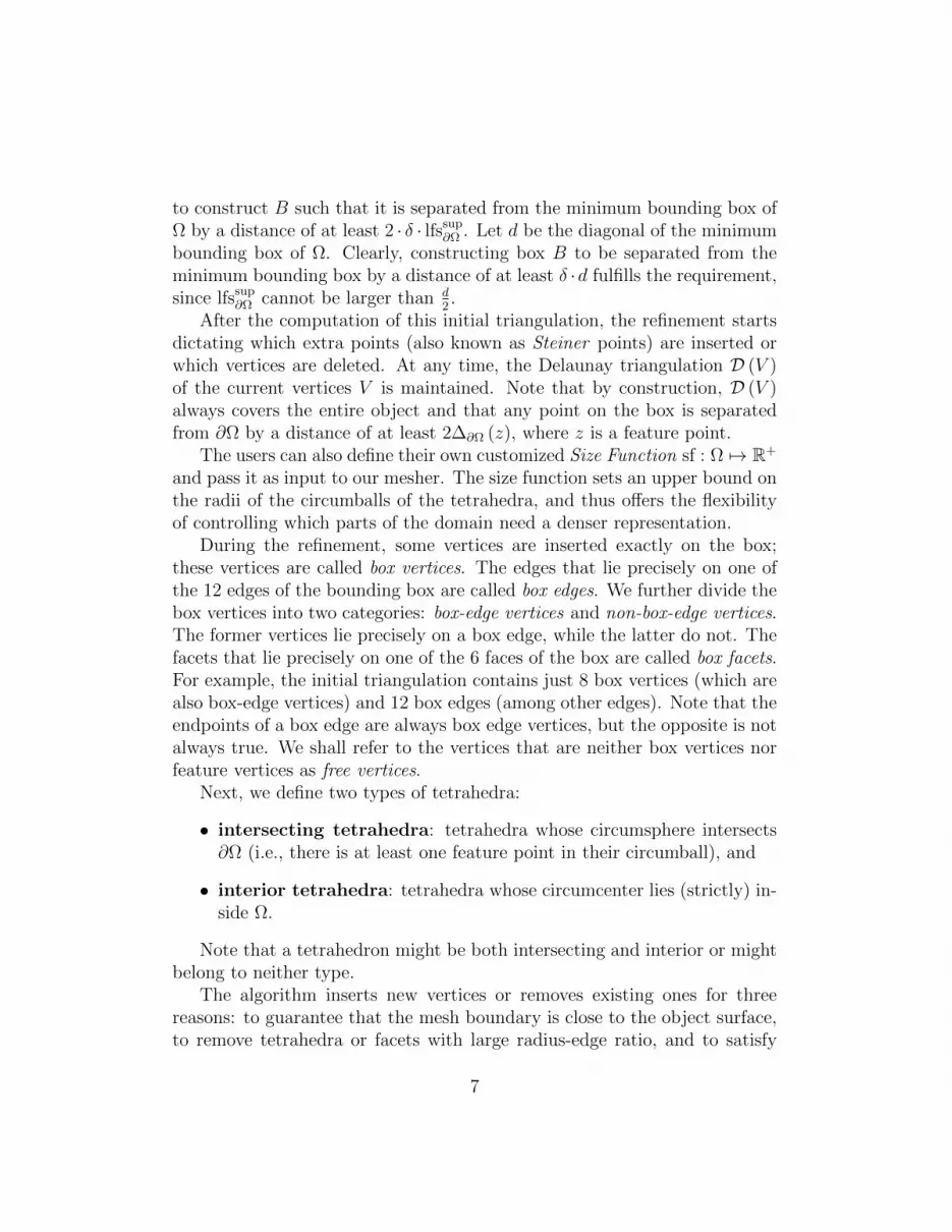
Algorithm 1: The mesh generation algorithm.1 Algorithm: Refine(I, δ, ρt, ρf , sf (·))
Input : I is the image containing Ω,δ is the parameter that determines how dense the surface sampling will be,
ρt (≥√√
3 + 2) is the target radius-edge ratio for the tetrahedra,ρf (≥ 1) is the target radius-edge ratio for the facets,sf (·) is the size function.
Output: A Delaunay mesh M that approximates ∂Ω well and is composed of tetrahedra with radius-edge ratioless than ρt and boundary facets with planar angles larger than 30.
2 Let V be the set of vertices inserted into the triangulation;3 Let D (V ) be the triangulation of the set V ;4 Let Intersecting and Interior be the set of the intersecting and interior tetrahedra in D (V ), respectively;
/* At this point, all the above sets are equal to the empty set. */
5 Insert the 8 vertices of a cubical box which contains Ω such that any point inserted on the box is separated fromany point z ∈ ∂Ω by a distance of at least 2 · δ · lfs∂Ω (z);
6 Update V,D (V ), Intersecting, and Interior ;7 while Intersecting ∪ Interior 6= ∅ do8 if Intersecting 6= ∅ then9 Pick a tetrahedron t ∈ Intersecting;
10 Compute steiner = cfp (c (t));11 if there is no feature vertex closer than δ · lfs∂Ω (steiner) to steiner then
/* R1 applies. */
12 else13 if r(t) ≥ 2 · δ · lfs∂Ω (steiner) then14 Compute steiner = c (t); /* R2 applies. */
15 if steiner lies outside the box then16 Compute steiner = c′ (t); /* Projection rules apply. */
17 end
18 else19 if t is adjacent to a restricted facet f , such that ρ (f) ≥ ρf or f ’s vertices do not lie on ∂Ω
then /* Since f is a restricted facet, f is necessarily incident to at least one
intersecting tetrahedron t. */
20 Compute steiner = csurf (f); /* R3 applies. */
21 else22 Intersecting = Intersecting \ t; /* No steiner point found. */
23 continue;
24 end
25 end
26 end
27 else /* Interior cannot be empty. */
28 if ρ (t) ≥ ρt or r(t) ≥ sf (c (t)) then29 Compute steiner = c (t); /* R4 or R5 apply. */
30 else31 Interior = Interior \ t; /* No steiner point found. */
32 continue;
33 end
34 end35 Insert steiner ;36 if steiner is a feature vertex then37 Delete all the free vertices that are closer than 2 · δ · lfs∂Ω (steiner) to steiner .38 end39 Update V , D (V ), Intersecting, and Interior ;
40 end41 Let the final mesh M be equal to the set of the tetrahedra in D (V ) whose circumcenter lies inside Ω;
10

4. Proof of Quality
In this section, we prove that if the target upper bound ρt for the radius-
edge ratio is no less than√√
3 + 2, then our algorithm terminates outputtingtetrahedra with radius-edge ratio less than ρt and boundary facets with pla-nar angles larger than 30 (see Theorem 2). Note that termination andquality are not compromised by any positive value of δ. Parameter δ affectsonly the fidelity guarantees (see Section 6).
Suppose that an element (tetrahedron or facet) t violates a rule Ri, wherei = 1, 2, 3, 4, 5, proj, where Rproj denotes the projection rules. That is, if tviolates R2, but its circumcenter lies on or outside the box, then we say thatt violates Rproj instead. t is called an Ri element. Ri dictates the insertionof a point p (and possibly the removal of free points). Point p is called an Ripoint. Although the initial 8 box corners inserted into the triangulation donot violate any rule, we shall refer to these corners as Rproj vertices as well.
Following similar terminology to [1, 27], we next define the insertionradius and the parent of a point p.
Definition 7 (Insertion radius). Let v be a vertex inserted into the triangula-tion. Right after the insertion of v (i.e., before any potential vertex removals),the insertion radius R(v) of v is equal to |vq|, where q is:
• v’s closest box vertex already inserted into the mesh, if v is a box vertex,
• v’s closest feature vertex already inserted into the mesh, if v is an R1vertex,
• v’s closest vertex already inserted into the mesh, otherwise.
Definition 8 (Parent). Let v be an Ri vertex inserted into the mesh becausean element (tetrahedron or facet) t violated Ri. The parent Par(v) of v is:
• an arbitrary box vertex, if t is a facet incident to at least one box vertex,
• the most recently inserted vertex of t, if t is a facet with ρ (f) < ρf ,
• the most recently inserted vertex of lmin (t), otherwise.
The following two Lemmata relate the insertion radii of a vertex v withthe distance between v and its neighbors.
11

rv
S(t)
c (t)
c′ (t) = v F
2D diskz ∈ ∂Ω
(a) c′ (t) is not a box-edge vertex.
rv
S(t)
c (t)
c′ (t) = v
F
2D disk
z ∈ ∂Ω
s
G
(b) c′ (t) is a box-edge vertex.
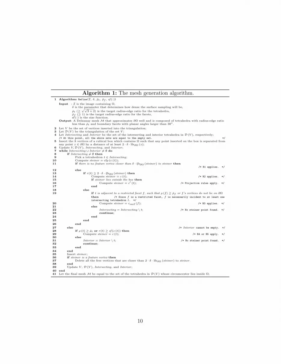
Figure 2: Illustration to the proof of Lemma 3.
Lemma 1. Let w be an R2, R3, R4, or an R5 vertex inserted into thetriangulation and let x be an arbitrary vertex already in the triangulation.Then, R(w) ≤ |wx|.
Proof. According to Definition 7, R(w) is the distance between w and itsclosest neighbor, say q. Therefore, R(w) = |wq| ≤ |wx|.
Lemma 2. Let w be an R1 vertex inserted into the triangulation and let x bean arbitrary feature vertex already in the triangulation. Then, R(w) ≤ |wx|.
Proof. According to Definition 7, R(w) is the distance between w and itsclosest feature vertex, say q. Therefore, R(w) = |wq| ≤ |wx|.
Lemma 3. Let v be a box vertex. Then, R(v) ≥ 2∆∂Ω (z), where z is theclosest feature point of v.
Proof. According to Definition 7, R(v) is the distance between v and itsclosest box vertex.
Initially, only the 8 box vertices of the bounding box are inserted. Byconstruction, no matter the order they are inserted, no box point is closer
12
than 2δlfssup∂Ω ≥ 2δlfs∂Ω (z) for any z ∈ ∂Ω. Therefore, the initial edges are
definitely larger than 4∆∂Ω (z) for any z ∈ ∂Ω, and the statement holds.During the course of refinement, a box point v is inserted either because
the circumcenter c (t) of an intersecting tetrahedron t lies on or outside thebox. According to the projection rules, c (t) is ignored, and its projectionc′ (t) is inserted instead.
See Figure 2 for two examples illustrating the insertion of a non box-edgevertex and a box-edge vertex. In both cases, consider the 2D disk (drawn inboth Figure 2a and Figure 2b) of the t’s sphere S(t) that contains c′ (t) andis perpendicular to the segment c (t) c′ (t). This disk partitions t’s circumballin two parts: the upper part that contains c (t) and the lower part thatintersects the interior of the box. From the empty ball property, we knowthat the insertion radius of c′ (t) cannot be less than the radius of the 2Ddisk. Let z be the closest feature point to c′ (t). Since t is an intersectingtetrahedron, z has to lie in the lower part of t’s circumball, which meansthat R(c′ (t)) ≥ |c′ (t) z|. By construction, however, |c′ (t) z| is larger than2δlfssup
∂Ω ≥ 2∆∂Ω (z), and the proof is complete.
Lemma 4. Let v be a box vertex. Then |vcfp (v)| ≤ R(v)√
3.
Proof. If v is a box vertex inserted because the circumcenter of an R2 elementlies on or outside the box, then the statement holds, because the proof ofLemma 3 directly suggests that |cfp (v) v| ≤ R(v).
Consider the case where the box vertex v is one of the initially inserted 8box corners. Note that the circumballs of all the resulting tetrahedra are thesame with the circumscribed ball of the box. Let us denote with r the lengthof the radius of that ball. Since that ball contains the whole box, we havethat |vcfp (v)| ≤ 2r. It is easy to show that r =
√3
2L, where L is the box’s
edge length edge. From Definition 7, we know that R(v) = L, and therefore,we obtain that |vcfp (v)| ≤ 2r = L
√3 = R(v)
√3.
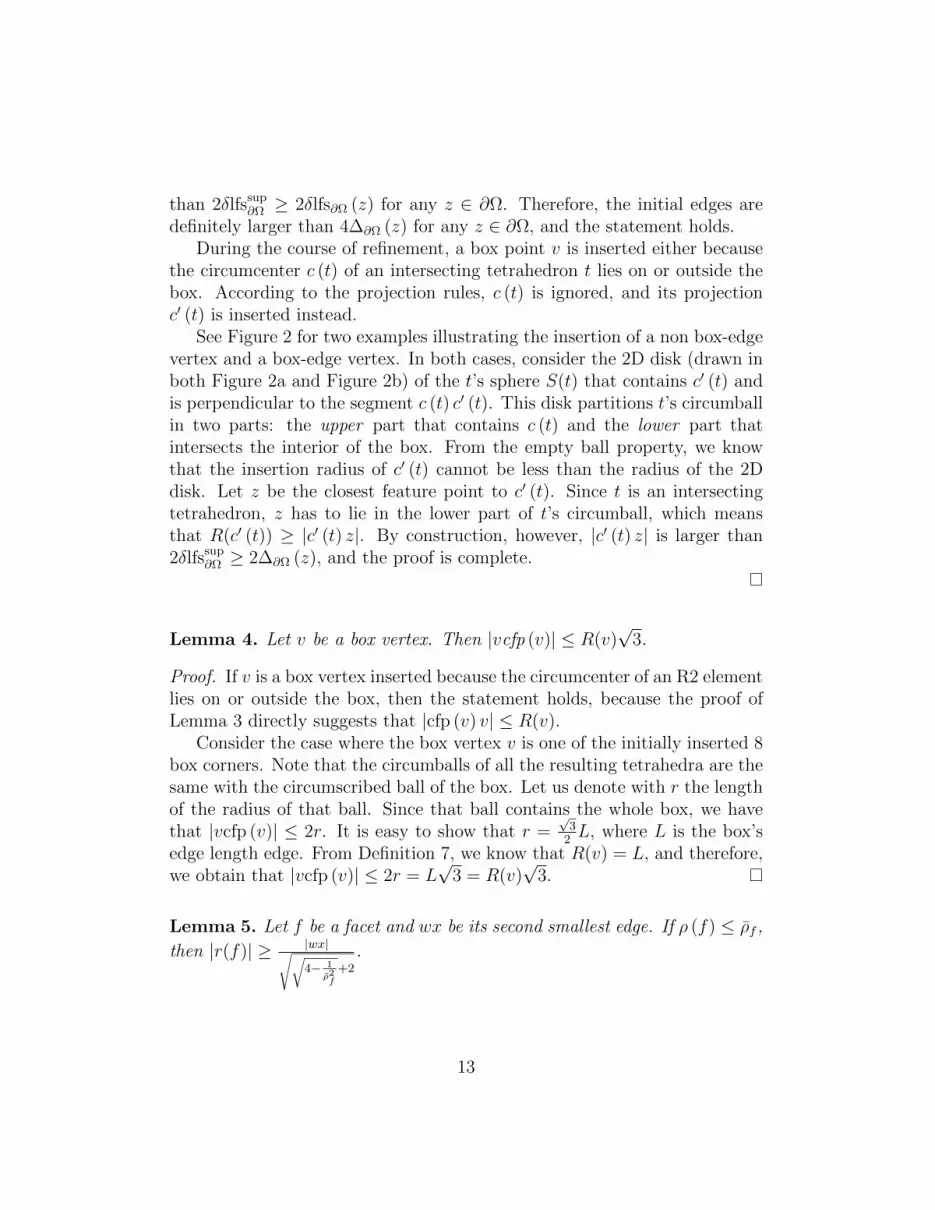
Lemma 5. Let f be a facet and wx be its second smallest edge. If ρ (f) ≤ ρf ,
then |r(f)| ≥ |wx|√√4− 1
ρ2f
+2
.
13
w
qx
c
b
θ
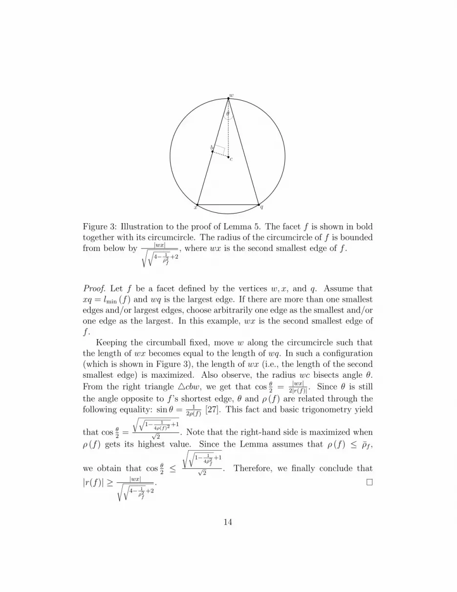
Figure 3: Illustration to the proof of Lemma 5. The facet f is shown in boldtogether with its circumcircle. The radius of the circumcircle of f is boundedfrom below by |wx|√√
4− 1
ρ2f
+2
, where wx is the second smallest edge of f .
Proof. Let f be a facet defined by the vertices w, x, and q. Assume thatxq = lmin (f) and wq is the largest edge. If there are more than one smallestedges and/or largest edges, choose arbitrarily one edge as the smallest and/orone edge as the largest. In this example, wx is the second smallest edge off .
Keeping the circumball fixed, move w along the circumcircle such thatthe length of wx becomes equal to the length of wq. In such a configuration(which is shown in Figure 3), the length of wx (i.e., the length of the secondsmallest edge) is maximized. Also observe, the radius wc bisects angle θ.
From the right triangle 4cbw, we get that cos θ2
= |wx|2|r(f)| . Since θ is still
the angle opposite to f ’s shortest edge, θ and ρ (f) are related through thefollowing equality: sin θ = 1
2ρ(f)[27]. This fact and basic trigonometry yield
that cos θ2
=
√√1− 1
4ρ(f)2+1
√2
. Note that the right-hand side is maximized when
ρ (f) gets its highest value. Since the Lemma assumes that ρ (f) ≤ ρf ,
we obtain that cos θ2≤
√√1− 1
4ρ2f
+1
√2
. Therefore, we finally conclude that
|r(f)| ≥ |wx|√√4− 1
ρ2f
+2
.
14

The following lemma sets a lower bound on the shortest edge introducedinto the mesh after the insertion of a point according to the five rules.
Lemma 6. Let v be inserted as dictated by the five rules and w be its parent.Then,
• R(v) ≥ ∆∂Ω (z), if v is an R1 or an R2 vertex, where z is the closestfeature point to v,
• R(v) ≥ min
R(w)√√4− 1
ρ2f
+2
, ρfR(w),∆∂Ω (v)
, if v is an R3 vertex and w
is a free or a box vertex,
• R(v) ≥ minρfR(w),∆∂Ω (w)
, if v is an R3 vertex and w is a feature
vertex,
• R(v) ≥ ρtR(w), if v is an R4 vertex,
• R(v) ≥ sf (v), if v is an R5 vertex.
Proof. We separate cases according to the type of v.
• Case 1: v is an R1 or an R2 vertex.
If R1 is triggered, then v is equal to z. According to Definition 7,R(v) is the distance between v and its closest feature vertex. Vertex v,however, is inserted only if v is separated from any other feature vertexby a distance of at least ∆∂Ω (v) = R(v), and the statement holds.
Otherwise, R2 applies for a tetrahedron t and v is equal to c (t). Ac-cording to Definition 7, R(v) is the distance between v and its clos-est neighbor. Because of the empty ball property, R(v) is at leastr(t) ≥ 2∆∂Ω (cfp (v)), and the statement holds.
• Case 2: v is an R3 vertex.
In this case, v is equal to the center csurf (f) of f ’s surface ball, wheref is the restricted facet that violates R3. According to Definition 7,R(v) is the distance between v and its closest neighbor. Since anysurface ball is empty of vertices in its interior (Remark 1), we know thatR(v) = |rsurf (f)|. The rest of this proof attempts to bound |rsurf (f)|from below. We separate three scenaria:
15

(a) First, consider the case where f is incident to at least on boxvertex. According to Definition 8, this box vertex can be the parent wof v. By construction, the distance between csurf (f) and w is at least2∆∂Ω (z) for any feature point z. Therefore, the surface radius is atleast 2∆∂Ω (v) > ∆∂Ω (v), and the statement holds.
(b) Second, consider the case where ρ (f) ≥ ρf . According to Defini-tion 8, w is the most recently inserted vertex incident to wq = lmin (f).Since ρ (f) is no less than ρf , |r(f)| = ρ (f) |lmin (f)| ≥ ρf |lmin (f)|.If w is not an R1 vertex, from Lemma 1, we get that |r(f)| ≥ ρf |lmin (f)| ≥ρfR(w).
If w is an R1 vertex and q is a feature vertex (that is, q is either an R1 oran R3 vertex), then from Lemma 2, we get that |r(f)| ≥ ρf |lmin (f)| ≥ρfR(w).
If w is an R1 vertex and q is a free vertex then q has to be separated fromw by a distance of at least 2∆∂Ω (w), because R1 deleted all the freepoints closer than 2∆∂Ω (w) to w. That means that |wq| ≥ 2∆∂Ω (w),
a fact that also bounds |r(t)| from below by |wq|2≥ ∆∂Ω (w).
(c) Lastly, consider the case where f ’s radius-edge ratio is less than ρf .Since R3 is triggered, f has to be incident to at least one free vertexq. According to Definition 8, w is the most recently inserted vertex off . If w is a feature vertex (i.e., w is either an R1 or an R3 vertex),then q must be separated from w by a distance of at least 2∆∂Ω (w),because w was inserted after q, and by R1 and R3, all the free pointscloser than 2∆∂Ω (w) to w were deleted. Since wq is an edge of f , the
radius of any surface ball of f has to be at least 2∆∂Ω(w)2
= ∆∂Ω (w) inlength. Otherwise, w is in fact a free vertex (i.e., it is an R2, R4, orR5 vertex).
Any vertex w of f is incident to f ’s shortest edge (say L1), or f ’ssecond shortest edge (say L2), or both. From Lemma 5, we have that
|r(f)| ≥ |L2|√√4− 1
ρ2f
+2
≥ |L1|√√4− 1
ρ2f
+2
. From Lemma 1, we finally get that:
|r(f)| ≥ R(w)√√4− 1
ρ2f
+2
.
• Case 3: v is an R4 vertex.
16

There has to be a tetrahedron t that violates R4, and therefore, |r(t)| ≥ρt |lmin (t)|. According to Definition 7, R(v) is the distance between vand its closest neighbor. Because of the empty ball property, R(v) =|r(t)| ≥ ρt |lmin (t)|. According to Definition 8, the parent w of v is themost recently inserted vertex of wq = lmin (t).
If w is not an R1 vertex, from Lemma 1, we get that ρt |lmin (t)| ≥ρtR(w).
If w is an R1 vertex and q is a feature vertex (that is, q is either an R1or an R3 vertex), then from from Lemma 2, we get that ρt |lmin (t)| ≥ρtR(w).
If w is an R1 vertex and q is a free vertex then q has to be separated fromw by a distance of at least 2∆∂Ω (w), because R1 deleted all the freepoints closer than 2∆∂Ω (w) to w. That means that |wq| ≥ 2∆∂Ω (w),
a fact that also bounds |r(t)| from below by |wq|2≥ ∆∂Ω (w).
• Case 4: v is an R5 vertex.
v is the circumcenter of a tetrahedron t with radius no less than sf (c (t)) =sf (v). According to Definition 7 and the empty ball property, however,the radius of t is equal to R(v).
The next Lemma shows that the boundary facets of the output mesh arein fact restricted facets.
Lemma 7. Let V be the set of vertices inserted into the triangulation. Theset ∂M of the boundary facets of the final mesh M is a subset of D|∂Ω (V ).
Proof. It follows directly from Definition 6. A facet f is a facet of the meshboundary, if it is incident upon a tetrahedron t1 whose circumcenter liesinside Ωi (see Section 2) and upon a tetrahedron t2 whose circumcenter lieseither outside Ωi or on its surface ∂Ωi. However, this means that the dualVoronoi edge e of f intersects ∂Ωi, and as a subsequence, e also intersects∂Ω (⊇ ∂Ωi). Hence, f belongs to D|∂Ω (V ).
17

ρt
ρt
ρt
ρt
∆∂Ω (z)
∆∂Ω (z)
∆∂Ω (z)
∆∂Ω (z)
∆∂Ω (z)
∆∂Ω (z)
1√√√√√
4− 1ρ2f
+2
1√√√√√
4− 1ρ2f
+2
1√√√√√
4− 1ρ2f
+2
ρf
ρf
ρf
ρf
sf
sfsf
R3 R4
R5
R1/R2/projection
Figure 4: Flow diagram depicting the relationship among the insertion radiiof the vertices inserted because of the rules, where the arrows point fromparents to their offspring. A solid arrow from Ri to Rj with label x impliesthat the insertion radius of an Rj point v is at least x times larger than theinsertion radius of its Ri parent w. The label of the dashed arrows is theabsolute value of R(v). No solid cycle should have a product less than 1.The dashed arrows break the cycle.
Theorem 2 (Termination and quality). Let ρf ≥ 1 and let
ρt ≥√√
4− 1ρ2f
+ 2(≥√√
3 + 2 ≈ 1.93)
. The algorithm terminates pro-
ducing tetrahedra of radius-edge ratio less than ρt and boundary facets ofplanar angles larger than 30.
Proof. Figure 4 shows the insertion radius of the inserted point as a fractionof the insertion radius of its parent, as proved in Lemma 3 and Lemma 6.An arrow from Ri to Rj with label x implies that the insertion radius ofan Rj point v is at least x times larger than the insertion radius of its Riparent w. The label of the dashed arrows is the absolute value of R(v), withsf denoting that the insertion radius of v is no less than sf (v). Note that the
18

labels of the dashed arrows depend on the local feature size of ∂Ω and thesize function sf, and as such are always positive constants.
Recall that during refinement, free vertices might be deleted (because ofR1 or R3). Nevertheless, such deletions of vertices are always preceded byinsertion of feature points. Considering the fact that feature vertices arenever deleted from the mesh, termination is guaranteed if we prove that theinsertion radii of the inserted vertices cannot approach zero. Clearly [1, 27],it is enough to prove that Figure 4 contains no solid cycle of product lessthan 1. By requiring ρf to be no less than 1 (cycle R3 → R3) and ρt to be
no less than
√√4− 1
ρ2f
+ 2 ≥√√
3 + 2 (cycle R3 → R4 → R3), no solid
cycle of Figure 4 has product less than 1, and termination is guaranteed.Upon termination, the tetrahedra reported as part of the mesh have cir-
cumcenters that lie inside Ω and therefore they cannot be skinny, becauseotherwise R4 would apply. This implies that any mesh tetrahedron hasradius-edge ratio less than ρt.
Since a boundary facet f is a restricted facet (by Lemma 7), R3 guaranteesthat the radius-edge ratio ρ (f) of f ’s diametral ball cannot be larger thanor equal to ρf . Also, note that ρ (f) is equal to 1
2 sin θ, where θ is the smallest
angle of f [27]. It follows that the planar angles are larger than 30.
5. Proof of Good Grading
In this Section, we show that the shortest edge connected to an insertedvertex v is proportional to v’s local feature size, a property that is alsoknown as good grading. Although good grading implies size optimality in2D domains [28], the same does not hold in general 3D domains, a mishapassociated to the fact that slivers are not provably eliminated. As explainedand demonstrated in [1], there are cases such that the local feature sizebecomes arbitrary close to zero, while there is a way to mesh the domainwith very few (and poor) elements. However, infinitesimal local feature sizemeans that even a very large number of elements satisfy the good gradingproperty, despite the fact that many fewer elements would suffice. This is apossible non size-optimal scenario.
Nevertheless, it is useful to show that parts of the domain with large localfeature sizes are meshed with larger and fewer elements than parts of smallerlocal feature sizes. We also wish to show that dense size functions on certain
19

parts will not affect considerably the density of vertices on other parts of thedomain.
Following similar terminology to [3], we define the general local featuresize and the general size function on a vertex v as follows:
Definition 9 (General Local Feature Size). The general local feature sizeglfs∂Ω (v) on a vertex v is defined as
glfs∂Ω (v) = infz∈∂Ω
|vz|+ lfs∂Ω (z) (2)
Definition 10 (General Size Function). The general size function gsf (v) ona vertex v is defined as
gsf (v) = infp∈Ω
|pv|+ sf (p)
(3)
The definition of glfs∂Ω (·) implies that vertices far from ∂Ω will tend tohave large general local feature sizes. In the case where the vertex lies onthe surface, the general local feature size coincides with the local feature size(see Definition 2) of the vertex, and it increases when the vertex lies far fromthe medial axis. The definition of gsf (·) implies that vertices close to partsof the domain on which the user-defined size function is small will evaluatethe general size function to a small number as well.
The following Remark states a few useful properties of the general localfeature size and the general size function:
Remark 2 (From [23, 29]). glfs∂Ω (·) and gsf (·) are 1-Lipschitz. Moreover,glfs∂Ω (z) = lfs∂Ω (v), ∀z ∈ ∂Ω.
Following the terminology of [1, 27], the density D (v) of a vertex v isdefined as:
D (v) =minglfs∂Ω (v) , gsf (v)
R(v)(4)
Our goal is to bound from above the density of all inserted vertices by aconstant depending only on Ω and the input parameters. Notice that sinceD (v) ≤ glfs∂Ω(v)
R(v)and D (v) ≤ gsf(v)
R(v), it is enough to bound from above either
glfs∂Ω(v)R(v)
or gsf(v)R(v)
.The following Lemma relates the insertion radius of a vertex with its
distance from its parent:
20

Lemma 8. Let v be an R3 or an R4 vertex inserted into the mesh and w beits parent. Then, R(v) = |vw|.
Proof. If v is an R3 or R4 vertex, then v is the center of an element t’scircumball or surface ball. According to Definition 8, the parent w of v isone vertex of t. Because of the empty circumball and surface ball property,Definition 7 implies that R(v) = |vw|.
The following Lemma relates the density of a vertex v with that of itsparent:
Lemma 9. Let v be an R3 or R4 vertex and R(v) ≥ c · R(w), where w =Par(v). Then
D (v) ≤ 1 +D (w)
c. (5)
Proof. The proof is similar to the proof of Lemma 6 in [27].Let w = Par(v). Since glfs∂Ω (·) and gsf (·) are 1-Lipschitz (see Re-
mark 2), we have that:
minglfs∂Ω (v) , gsf (v) ≤ min|vw|+ glfs∂Ω (w) , |vw|+ gsf (w)= |vw|+ minglfs∂Ω (w) , gsf (w)= R(v) + minglfs∂Ω (w) , gsf (w) (from Lemma 8)
= R(v) +R(w)D (w) (from Equation (4))
≤ R(v) + R(v)c D (w) ,
and the result follows by dividing both sides by R(v).
Before we proceed to the proof of good grading, we need two auxiliaryLemmata:
Lemma 10. Let v be an R2 vertex. Then, |vcfp (v)| ≤ R(v).
Proof. Vertex v is an R2 vertex because of an intersecting tetrahedron t.Since t is an intersecting tetrahedron and v is the center of t, we have that|vcfp (v)| ≤ |r(t)|. Definition 7, however, implies that |r(t)| = R(v), and thestatement holds.
Lemma 11. Let v be a vertex inserted into the mesh. Then,
• D (v) ≤ 1+δ√
3δ
, if v is an R1, R2, or a box vertex,
• D (v) ≤ 1+δδ
, if v is an R3 vertex and R(v) ≥ min∆∂Ω (w) ,∆∂Ω (v),where w = Par(v) ∈ ∂Ω, and
21

• D (v) ≤ 1, if v is an R5 vertex.
Proof. We separate cases.Let v be an R1 vertex. According to the flow diagram of Figure 4, we
have that R(v) ≥ ∆∂Ω (cfp (v)) = ∆∂Ω (v) = δ · lfs∂Ω (z). From Remark 2, we
have that R(v) ≥ δ · lfs∂Ω (z) = δ · glfs∂Ω (z), giving that D (v) ≤ 1δ≤ 1+δ
√3
δ,
and the statement holds.Let v be an R2 or a box vertex. According to the flow diagram, R(v) ≥
∆∂Ω (cfp (v)) = δ·lfs∂Ω (cfp (v)) = δ·glfs∂Ω (cfp (v)), and from the fact that thegeneral local feature size is 1-Lipschitz, we have thatR(v) ≥ δ (glfs∂Ω (v)− |vcfp (v)|).From Lemma 4 and Lemma 10, we know that |vcfp (v)| ≤ R(v)
√3. There-
fore, we obtain that R(v) ≥ δ(glfs∂Ω (v)−R(v)
√3). Dividing both sides by
R(v) finally gives that D (v) ≤ 1+δ√
3δ
, and the statement holds.Let v be an R3 vertex and R(v) ≥ ∆∂Ω (v) = δ · lfs∂Ω (v). It follows
directly that D (v) ≤ 1δ< 1+δ
δ.
Let v be an R3 vertex and R(v) ≥ ∆∂Ω (w), where w ∈ ∂Ω is the parentof v. From Remark 2, we obtain that R(v) ≥ ∆∂Ω (w) = δ · lfs∂Ω (w) =δ · glfs∂Ω (w) ≥ δ (glfs∂Ω (v)− |vw|). From Definition 8, w is one of thevertices of a restricted facet whose surface ball has v as the center. Fromthe empty surface ball property and Definition 7, we know that R(v) = |vw|.Therefore, R(v) ≥ δ (glfs∂Ω (v)−R(v)). Dividing both sides by R(v) finallygives that D (v) ≤ 1+δ
δ, and the statement holds.
Let v be an R5 vertex. According to the flow diagram, all the arrowspointing to R5 are dashed and labeled as sf. The label of dashed arrowsis the absolute value of R(v) and therefore, R(v) ≥ sf (v). Since, however,gsf (v) = inf
p∈Ω
|pv|+sf (p)
≤ |vv|+sf (v) = sf (v), we get that R(v) ≥ gsf (v),
and the proof is complete.
Finally, the following Theorem proves that our algorithm achieves goodgrading:
Theorem 3 (Good Grading). Let ρf be strictly larger than 1 and let ρt be
strictly larger than X =
√√4− 1
ρ2f
+ 2(≥√√
3 + 2 ≈ 1.93)
. Let v be an
Ri vertex inserted into the mesh, i = 1, 2, 3, 4, 5, proj. Then, right after itsinsertion, its density D (v) is bounded from above by a fixed constant Di > 0.
Proof. This theorem will be proved via induction.
22

Initially, only the 8 box corners are inserted into the triangulation. Ac-cording to Lemma 11, the induction basis holds, if
Dproj =1 + δ
√3
δ. (6)
For the induction hypothesis, assume that the density D (w) of v’s parentRj vertex w is bounded from above by Dj, where j = 1, 2, 3, 4, 5, proj. Weneed to show that one constant Di bounds from above the density of Ri
vertex v, where i = 1, 2, 3, 4, 5, proj.We separate cases according to the type of v:
• v is an R1, R2, or a box vertexAccording to Lemma 11, the insertion radius of v is bounded fromabove by 1+δ
√3
δ. Therefore, no matter what the parent of v is, the
induction step holds, if
D1 = D2 = Dproj =1 + δ
√3
δ. (7)
• v is an R5 vertexSimilarly to the case above, Lemma 11 suggests that no matter whatthe parent of v is, the induction step holds, if
D5 = 1. (8)
• v is an R4 vertexFrom the flow diagram, all the arrows pointing to R4 are labeled with ρt.Therefore, from Lemma 9 and Lemma 6, we get that D (v) ≤ 1 + D(w)
c,
with c equal to ρt for any parent w. Thus, the induction step wouldbe proved, if D4 was set to a value that satisfied all the followinginequalities:
1 +D1
ρt≤ D4 (9)
1 +D3
ρt≤ D4 (10)
23

1 +D4
ρt≤ D4 (11)
1 +D5
ρt= 1 +
1
ρt≤ D4 (12)
Observe that the D5 term in Inequality (12) is replaced by 1, accordingto Equality (8).
• v is an R3 vertexAccording to Lemma 11, D (v) is bounded from above by 1+δ
δfor the
relationships of Figure 4 that are depicted by the dashed arrows point-ing to R3. Therefore, for the induction step to be proved, D3 has tosatisfy at least the following inequality:
1 + δ
δ≤ D3 (13)
For the rest of the relationships (i.e., solid arrows), we know from
Lemma 9 and Lemma 6 that D (v) ≤ 1 + D(w)c
, where c is equal to
ρf if w is an R3 vertex or equal to min
1X, ρf
if w is an R1, R2,
Rproj, R4 or R5 vertex.
Therefore, the induction step would be proved, if D3 was set to a valuethat satisfied also the following inequalities:
1 +D1 max
X,
1
ρf
= 1 +D1X ≤ D3 (14)
1 +D3
ρf≤ D3 (15)
1 +D4 max
X,
1
ρf
= 1 +D4X ≤ D3 (16)
1 +D5 max
X,
1
ρf
= 1 +X ≤ D3 (17)
24

Observe that X is always larger than 1ρf
when ρf > 1 and that is
why the 1ρf
term is eliminated from Inequalities (14), (16), and (17).
Also, the D5 term in Inequality (17) is replaced by 1, according toEquality (8).
Putting it all together and simplifying the results, Inequalities (9)- (17)above are simultaneously satisfied by choosing:
D4 = max
ρt + 1
ρt −X,δ (ρt + 1) +X
(1 + δ
√3)
δρt,ρt (ρf − 1) + ρfρt (ρf − 1)
(18)
and
D3 = max
δ +X
(1 + δ
√3)
δ,δρt (1 +X) +X
(1 + δ
√3)
δρt,
ρfρf − 1
,ρt (1 +X)
ρt −X
(19)
Equalities (6), (7), (8), (18), and (19) satisfy both the induction basisand the induction step for any number and type of vertices, and therefore,the proof is complete.
6. Proof of Fidelity
In this section, we derive an upper bound for δ, such that the boundaryof the final mesh is a provably good topological and geometric approximationof ∂Ω. Our goal is to prove that the mesh boundary ∂M (see Definition 6) isequal to D|∂Ω (E) for E a 0.09-sample of ∂Ω (see Theorem 4 of this section).To see why this is enough, recall that from Theorem 1, the restriction of a0.09-sample of ∂Ω to ∂Ω is a good topological and geometric approximationof ∂Ω.
First, we show that δ directly controls the density of the feature vertices.Let V be the set of vertices in the triangulation and E be equal to V ∩ ∂Ω.
Lemma 12. Let δ < 14. Then E is a 5δ
1−4δ-sample of ∂Ω.
25

S(t)
p
p′
c
v
Figure 5: Illustration to the proof of Lemma 12.
Proof. Recall that upon termination, there is no tetrahedron for which R1,R2, R3, R4, or R5 apply.
See Figure 5. Let p be an arbitrary point on ∂Ω. Since D (V ) covers allthe domain, point p has to lie on or inside the circumsphere of a tetrahedront (not shown). Hence, t is an intersecting tetrahedron. Let point p′ be thefeature point closest to c (t). Note that |c (t) p| ≥ |c (t) p′| and therefore p′
lies on or inside t’s circumsphere. We also know that t’s circumradius has tobe less than 2∆∂Ω (p′), since otherwise R2 would apply for t. Therefore, wehave the following:
|pp′| < 2r(t) (because both p and p′ lie on or inside B(t))< 4∆∂Ω (p′) (because of R2)≤ 4δ (|pp′|+ lfs∂Ω (p)) (from Inequality (1)),
and by reordering the terms, we obtain that:
|pp′| < 4δ
1− 4δlfs∂Ω (p) , with δ <
1
4. (20)
Moreover, there must exist a feature vertex v in the triangulation closerthan ∆∂Ω (p′) = δ · lfs∂Ω (p′) to p′, since otherwise R1 would apply for t.Hence, |vp′| < δ · lfs∂Ω (p′), and using Inequality (1), we have that:
|vp′| < δ (|pp′|+ lfs∂Ω (p)) (21)
26

Applying the triangle inequality for 4pvp′ yields the following:
|pv| ≤ |pp′|+ |vp′|< |pp′|+ δ (|pp′|+ lfs∂Ω (p)) (from Inequality (21))= |pp′| (1 + δ) + δ · lfs∂Ω (p)< 4δ
1−4δlfs∂Ω (p) (1 + δ) + δ · lfs∂Ω (p) (from Inequality (20))
=(
4δ(1+δ)1−4δ
+ δ)
lfs∂Ω (p)
= 5δ1−4δ
lfs∂Ω (p) ,
and the proof is complete.
Recall from Section 2 that the multi-tissue object Ω could be described
as a union of materials Ω =n⋃i
Ωi. Let us denote by Ωji , the jth connected
component of a specific tissue Ωi, j = 1, . . . ,m.Similar to Definition 4, D|∂Ωji
(V ) denotes the set of those facets in the De-
launay triangulation of the vertices in V whose dual Voronoi edge intersects
the surface ∂Ωji of Ωj
i . Also, note that ∂Ω =n⋃i
m⋃j
∂Ωji .
From Lemma 12 and Definition 3, the following Corollary follows:
Corollary 1. Let δ ≤ 0.095.36≈ 0.0168 and let Ej
i = V ∩ ∂Ωji . Then, Ej
i is a
0.09-sample of ∂Ωji .
As we have already mentioned in Section 3, the final mesh M reportedconsists of tetrahedra whose circumcenter lies inside Ω. Let Mj
i be the setof tetrahedra whose circumcenter lies inside Ωj
i .Similar to Definition 6, ∂Mj
i denotes the set of the boundary facets ofsubmesh Mj
i . That is, ∂Mji contains the facets incident to two tetrahedra
such that one tetrahedron has a circumcenter lying inside Ωji and the other
has a circumcenter lying either outside Ωji or on ∂Ωj
i .
Lemma 13. Let t be an intersecting tetrahedron whose circumball B(t) con-tains a point m of ∂Ω’s medial axis. Then, δ > 1
4.
Proof. Upon termination, rule R2 cannot apply for any tetrahedron. There-
27
fore, we have the following:
2 · δ · lfs∂Ω (cfp (c (t))) > |r(t)| (from R2)
≥ |cfp(c(t))m|2 (since m and cfp (c (t)) lie inside B(t))
≥ lfs∂Ω(cfp(c(t)))2 (since m is on the medial axis) ⇒
δ > 14 .
Lemma 14. Let δ ≤ 14. Any facet f ∈ ∂Mj
i belongs to D|∂Ωji(V ) and has its
vertices on ∂Ωji .
Proof. Since f belongs to ∂Mji , f is incident to two tetrahedra t1, t2 ∈ D (V ),
such that the circumcenter of t1 lies inside Ωji and the circumcenter of t2 lies
outside Ωji or ∂Ωj
i . However, this means that the Voronoi edge of f intersects∂Ωj
i , and therefore, f ∈ D|∂Ωji(V ). This completes the first part.
For the second part and for the sake of contradiction, assume that thereis at least one vertex v of f that does not lie on ∂Ωj
i , but on another ∂Ωj′
i′ .Consider the tetrahedron t1, one of the two tetrahedra incident to f withcircumcenter lying inside Ωj
i . Since v lies on ∂Ωj′
i′ , the circumball B(t1) of t1intersects ∂Ω in more than one connected component. According to Lemma7 of Amenta and Bern [17], this implies that B(t) contains a point m ofthe medial axis of ∂Ω. Moreover, observe that t1 is in fact an intersectingtetrahedron. From Lemma 13, we finally get that δ > 1
4. However, this raises
a contradiction, since δ is assumed to be no larger than 14.
The next two Lemmas prove a few useful properties for the meshM andits boundary ∂M. Our goal is to show that ∂Mj
i is always non-empty anddoes not have boundary (Lemma 16), a fact that will be used for proving thefidelity guarantees (Theorem 4).
Lemma 15. Let δ ≤ 14. Then, Mj
i 6= ∅.
Proof. For the sake of contradiction, assume thatMji is empty. That means
that there is no tetrahedron whose circumcenter lies inside Ωji . Since the
triangulation D (V ) covers all the domain, the circumballs of the tetrahedrain D (V ) also cover the tissue Ωj
i . Therefore, there has to be a circumballB(t) (t ∈ D (V )) which contains a point m on the medial axis of ∂Ωj
i , such
28

that m lies inside Ωji . By our assumption, the circumcenter c (t) cannot lie
inside Ωji . Therefore, t is an intersecting tetrahedron. From Lemma 13, we
finally get that δ > 14. However, this raises a contradiction, since δ is assumed
to be no larger than 14.
Lemma 16. Let δ ≤ 14. Then ∂Mj
i is a non-empty set and does not haveboundary.
Proof. The fact that ∂Mji is a non-empty set follows directly from Lemma 15:
sinceMji cannot be empty, its boundary ∂Mj
i cannot be empty too. For theother part, since ∂Mj
i is the boundary of a set of tetrahedra, it cannot haveboundary.
The following Theorem proves the fidelity guarantees achieved by ouralgorithm:
Theorem 4. Let δ = 0.0168. Then the mesh boundary ∂M is a 2-manifoldambient isotopic to ∂Ω and the 2-sided Hausdorff distance between the meshboundary and ∂Ω is O(δ2).
Proof. By Theorem 1, it is enough to prove that ∂M is the restriction to∂Ω of the Delaunay triangulation of a 0.09-sample. We will, in fact, showthat the boundary ∂Mj
i of the submesh Mji is equal to D|∂Ωji
(Eji
)(recall
that Eji is equal to V ∩ ∂Ωj
i ) which is the restriction to ∂Ωji of the Delaunay
triangulation of a 0.09-sample of ∂Ωji , by Corollary 1. This is enough, since
this would prove that the boundary of each submesh Mji is an accurate
representation of the interface ∂Ωji , for any i and j.
Let f be a facet in ∂Mji . From Lemma 14, we know that f ∈ D|∂Ωji
(V )
that f ’s vertices lie on ∂Ωji . Let B be the surface ball of f . From Definition 5,
the interior int (B) of B is empty of vertices in V . Therefore, int (B) is emptyof vertices in V ∩∂Ωj
i also. Without loss of generality, assume that the verticesin V are in general position. Since there is a ball B that circumscribes f anddoes not contain vertices of V ∩∂Ωj
i in its interior, f has to appear as a simplexin D
(V ∩ ∂Ωj
i
). Since the center of B lies on ∂Ωj
i , then the Voronoi dual of
f intersects ∂Ωji in D|∂Ω
(V ∩ ∂Ωj
i
), as well. Hence, ∂Mj
i ⊆ D|∂Ωji
(V ∩ ∂Ωj
i
).
For the other direction, we will prove that ∂Mji cannot be a proper subset
of D|∂Ωji
(V ∩ ∂Ωj
i
), and therefore, equality between these two sets is forced.
29

Toward this direction, we will prove that any proper non-empty subset ofD|∂Ωji
(V ∩ ∂Ωj
i
)has boundary; this is enough, because we have proved in
Lemma 16 that ∂Mji is non-empty and does not have boundary.
Since V ∩ ∂Ωji meets the requirements of Theorem 1, D|∂Ωji
(V ∩ ∂Ωj
i
)is a 2-manifold without boundary. Therefore, any edge in D|∂Ωji
(V ∩ ∂Ωj
i
)is incident to exactly two facets of D|∂Ωji
(V ∩ ∂Ωj
i
). Since any proper non-
empty subset A of D|∂Ωji
(V ∩ ∂Ωj
i
)has fewer facets, A contains at least an
edge e incident to only one facet. However, this implies that e belongs to theboundary of A, and the proof is complete.
7. Implementation details
We used the Insight Toolkit (ITK) for image processing [30]. ITK pro-vides, among others, the implicit function f that describes object Ω to bemeshed (see Section 2). Specifically, given a real point p, f returns 0 if thevoxel enclosing p is in the background, or it returns the identifier i of thetissue Ωi if that voxel belongs to Ωi, i = 1, . . . , n. In order to compute theclosest feature point function cfp (p) and identify the cloud of points lying on∂Ω, we make use of the Euclidean Distance Transform (EDT) as implementedin ITK and presented in [31]. Specifically, the EDT returns the boundary
voxel p′ which is closest to p. Then, we traverse the ray−→pp′ and we compute
the intersection between the ray and ∂Ω by interpolating the positions wheref changes value [20]. The actual mesh generator was built on top of the Com-putational Geometry Algorithms Library (CGAL) [32]. CGAL offers flexibledata structures for Delaunay point insertions and removals and robust exactgeometric predicates.
The rest of this section describes important implementation aspects.
7.1. Medial Axis Approximation
Recall that rules R1 and R2 make an extensive use of lfs∂Ω (·), and there-fore, knowledge about the medial axis is needed.
Since the computation of the exact medial axis is a difficult problem [33,34], we seek a good (for our purposes) approximation of it. Precisely, we
are interested in computing lfs∂Ω (p): the approximation of lfs∂Ω (p), wherep ∈ ∂Ω.
30
Remark 3. In this subsection, we do not alter the fidelity guarantees ofTheorem 4, since the theorem assumes that lfs∂Ω (·) is known and accurate;in this subsection, we attempt to provide a fast way to approximate lfs∂Ω (·).
For an excellent review of image-based medial axis approximation meth-ods, see the work of Coeurjolly and Montanvert [35]. The authors also de-scribe an optimal algorithm (MAEVA1) for the computation of the medialaxis, which is a free implementation to download. We found out, however,that although the method is fast, the resulted discrete medial axis was notaccurate enough for our purposes. We attribute this behavior to the factthat image-based methods do not realize the underlying shape; they com-pute the medial axis of volumetric data, which contains discontinuities andthus, renders the computation unstable.
Amenta et al. [18] and Dey and Zhao [33] (and the references therein)consider methods that given a set of sample points on the surface, they ap-proximate the medial axis from their Voronoi diagram. Their key conceptis the Pole of a feature vertex, a technique that we integrate into our al-gorithm in order to compute lfs∂Ω (·). Boissonnat and Oudot [19] describea two-phase algorithm that is able to approximate the medial axis basedon the notion of the Lambda-Medial Axis [36]. The Lambda-Medial Axismakes weaker assumptions about the sample and as such, it is suitable fornoisy data. Nevertheless, we found that the Pole technique is easier to im-plement and quite robust for our purposes in all the input images we tried.It should also be mentioned that both the Pole and the Lambda-Medial Axistechnique focus on surface recovery and not volume meshing. That meansthat they assume that only vertices on the isosurface are allowed (i.e., thesample). This is not the case in this work, since the quality criteria mightdictate the insertion of vertices in the interior of the domain. As we explainbelow, this difference necessitates the simultaneous maintenance of a secondtriangulation.
Let E be a vertex set on ∂Ω and consider the voronoi vertices of thevoronoi cell of a feature vertex v ∈ E. The voronoi vertices inside Ω (ifany) are called internal and the rest (if any) external. Amenta et al. [18]shows that if E is dense, the internal pole (i.e., the furthest from v internalvoronoi vertex) is close to the medial axis contained in Ω, and the externalpole (i.e., the furthest from v external voronoi vertex) is close to the medial
1http://liris.cnrs.fr/david.coeurjolly/doku/doku.php?id=code:maeva
31

axis contained in the complement of Ω. Therefore, the poles of each samplepoint form a good discrete approximation of the medial axis.
The problem with the poles (as a good approximation of the medial axis)is that E has to be a dense sample of the surface; however, our algorithmneeds the approximation of the medial axis, so it can create a graded sampleE. Recall that we do not assume that a starting sample set is known a priori.In fact, when the algorithm starts, there is not a even a single feature vertexinserted into the triangulation. In order to resolve this cyclic dependency,our algorithm alternates between two modes: a “uniform” and a “graded”.
Specifically, the algorithm maintains a second triangulation D (Z) (to-gether with the triangulation D (V ), see Section 3) which contains only fea-
ture vertices. To compute lfs∂Ω (z), z is inserted into the current set of featurevertices Z, and D (Z) is updated. Next, the poles of z are computed fromD (Z), and the distance from z to its closest pole is returned as the ap-proximation of the distance from z to the medial axis. Clearly, in the earlystages of the refinement, Z is a very sparse sample set, and, therefore, thepoles of z ∈ Z are not to be trusted as a good approximation of the medialaxis. Note, however, that these poles can only be further from z, than thepoles computed at a much denser sample set. In other words, when Z issparse, lfs∂Ω (z) gives a larger value than it should (i.e, lfs∂Ω (z) is larger thanlfs∂Ω (z)). This has severe consequences, since it is possible for the resultingsample not to be as dense as it should.
For this reason, instead of returning just the value of lfs∂Ω (z), we choose
to return the following quantity: minλ, lfs∂Ω (z), where λ will be specified
shortly. When lfs∂Ω (z) is too large (i.e., larger than λ), the value of λ isreturned. Parameter λ acts as a safety net and simulates the uniform modeof the algorithm: in the worst case, a uniform sample set will be generated,whose density depends on λ. Note that the uniform mode is triggered mostlyin the early stages of the algorithm. Later on, more and more feature ver-tices are inserted into the triangulation, and the medial axis is sufficientlydescribed by the poles; and this is when the graded mode of the algorithmis activated.
Specifying a value for λ is not intuitive. If λ is small, then the approxima-tion of the medial axis would be more accurate, but the graded mode wouldbe activated fewer times, sacrificing in this way a well-graded surface mesh.On the other hand, if λ is large, then we would expect to see better grading,but it is likely for the approximation of medial axis to be so bad (i.e., it is
32
likely that lfs∂Ω (·) is too large), such that the graded mode would fail to cap-ture the curvature of ∂Ω. Nevertheless, extensive experimental evaluation onboth synthetic and real medical images has shown that in most cases, settingλ to a value 12 times the size of the voxel suffices.
Note that if the users are not interested in achieving grading along thesurface, the second triangulation D (Z) is not needed at all, since they could
define lfs∂Ω (p) to be simply equal to λ.
7.2. Dihedral angle improvement
Provable theoretical guarantees on the minimum and maximum dihedralangles are outside the scope of this paper. Nevertheless, for practical pur-poses, we felt that the issue of sliver removal and dihedral angle improvementshould be addressed.
We could apply the sliver exudation technique [8] in order to improvethe dihedral angles. Edelsbrunner and Guoy [37], however, have shown thatin most cases sliver exudation does not remove all poor tetrahedra: ele-ments with dihedral angles less than 5 survive. The random perturbationtechnique [12] offers very small guarantees and sometimes requires many(random) trials for the elimination of a single sliver as reported in [16].
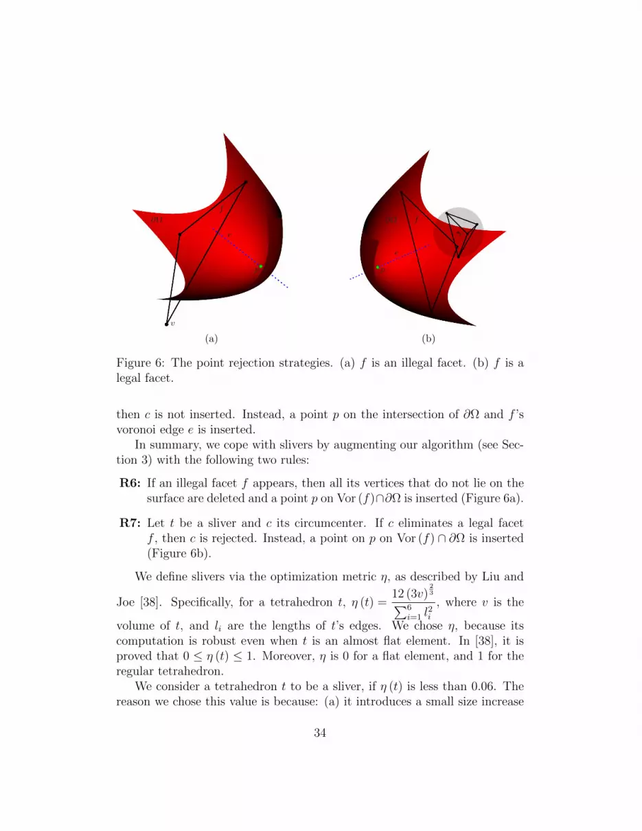
A straightforward and inexpensive way to eliminate slivers is to try to splitthem by inserting their circumcenter. Shewchuk [1] shows that this techniqueworks when the slivers are far away from the mesh boundary. However, whenslivers are close to the mesh boundary, the newly inserted points alter theboundary triangles. In fact, the boundary triangles might not have theirvertices on the surface any more, or might not even belong to the restrictedtriangulation. In this subsection, we propose point rejection strategies thatprevent the insertion of points which hurt fidelity.
Our algorithm first tries to convert illegal facets to legal ones. We definelegal facets to be those restricted facets whose vertices lie precisely on ∂Ω.Conversely, a restricted facet with at least one vertex not lying on ∂Ω iscalled an illegal facet.
Let f be an illegal facet and e its voronoi edge (see Figure 6a). Recallthat e has to intersect ∂Ω (see Section 2) at a point p. Any vertex v of fwhich do not lie precisely on ∂Ω is deleted from the triangulation, while pointp is inserted.
In addition, the algorithm tries to keep in the Delaunay triangulation asmany legal facets as possible. Let c be the circumcenter of a sliver consideredfor insertion. If the insertion of c eliminates a legal facet f (see Figure 6b),
33
e
p
f
v
∂Ω
(a)
e
p
c
f∂Ω
(b)
Figure 6: The point rejection strategies. (a) f is an illegal facet. (b) f is alegal facet.
then c is not inserted. Instead, a point p on the intersection of ∂Ω and f ’svoronoi edge e is inserted.
In summary, we cope with slivers by augmenting our algorithm (see Sec-tion 3) with the following two rules:
R6: If an illegal facet f appears, then all its vertices that do not lie on thesurface are deleted and a point p on Vor (f)∩∂Ω is inserted (Figure 6a).
R7: Let t be a sliver and c its circumcenter. If c eliminates a legal facetf , then c is rejected. Instead, a point on p on Vor (f) ∩ ∂Ω is inserted(Figure 6b).
We define slivers via the optimization metric η, as described by Liu and
Joe [38]. Specifically, for a tetrahedron t, η (t) =12 (3v)
23∑6
i=1 l2i
, where v is the
volume of t, and li are the lengths of t’s edges. We chose η, because itscomputation is robust even when t is an almost flat element. In [38], it isproved that 0 ≤ η (t) ≤ 1. Moreover, η is 0 for a flat element, and 1 for theregular tetrahedron.
We consider a tetrahedron t to be a sliver, if η (t) is less than 0.06. Thereason we chose this value is because: (a) it introduces a small size increase
34

(about 15%) over the mesh obtained without our sliver removal heuristic (i.e.,without rules R6 and R7), and (b) it introduces a negligible time overhead.In the Experimental Section 8, we show that this 0.06 bound corresponds tomeshes consisting of tetrahedra with dihedral angles between 4.6 and 171.
Note that R6 and R7 never remove feature vertices; on the contrary, theymight insert more to “protect” the surface. Hence, they do not violate The-orem 4: the mesh boundary continues being equal to the restricted Delaunaytriangulation D|∂Ω (V ∩ ∂Ω), and therefore a good approximation of the sur-face. In order not to compromise termination (and the guarantees we give forthe radius-edge ratio and the boundary planar angles), if R6 or R7 introducean edge shorter than the shortest edge already present in the mesh, then theoperation is rejected and the sliver in question is ignored.
We experimentally found that the point rejection strategies were able togenerate tetrahedra with angles more than 4.5 and less than 171. We em-phasize that neither fidelity (see Theorem 4) nor termination (see Theorem 2)is compromised with this heuristic.
8. Experimental Evaluation
This section presents the final meshes generated by our algorithm onsynthetic and real medical data. All the experiments were conducted on a 64bit machine equipped with a 2.8 GHz Intel Core i7 CPU and 8 GB of mainmemory. For the 3D visualization of the final meshes, we used ParaView [39],an open source visualization application.
Although the fidelity guarantees we give hold for a very small value of δ(see Theorem 4), we wanted to see if our algorithm works well for much largervalues of δ. Specifically, for all the experiments, we set δ to 2, i.e., we setδ to a value about 200 times larger than Theorem 4 recommends. A largervalue of δ also implies that the size of the output mesh is smaller. Small-size meshes are desirable for two reasons: first, because the mesh generationexecution time is considerably less (as it can be seen below, see Table 1a),and second, because finite element simulations [40, 41] on them run faster.We observed that even though the fidelity guarantees proved in Section 6do not hold for large δ, the results in fact are pretty good. (We should alsonote that in some applications fidelity is not that important. For instance,a study on the impact of δ for the non-rigid registration problem [42] showsthat the accuracy and speed of the solver is not very sensitive to fidelity.)
35
(a) sf1 (·): the radii are smaller than 5mm.
(b) sf2 (·): the radii are smaller than 1mm.
(c) sf3 (·): the radii are smaller than 5mm for z ≥ 0 and smaller than1mm for z < 0.
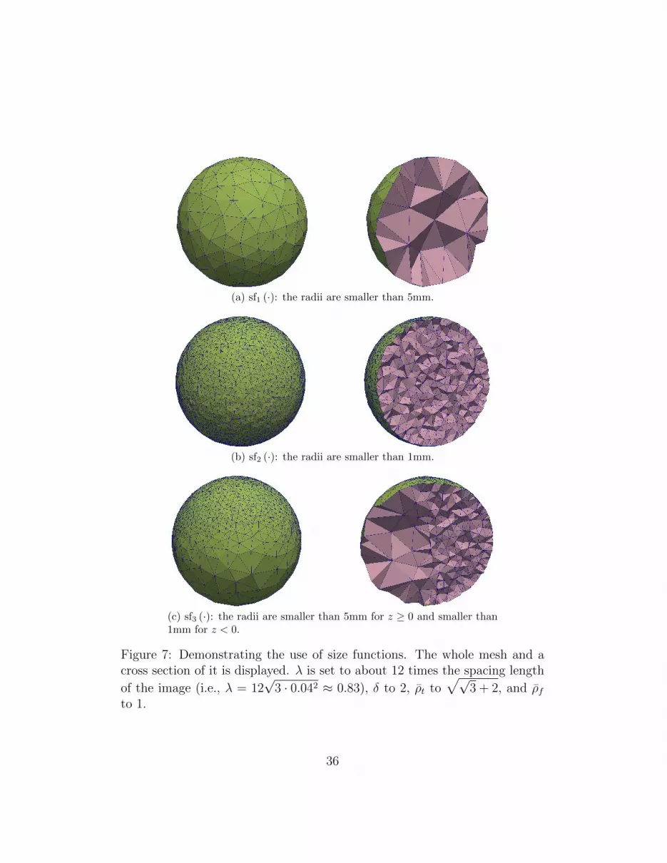
Figure 7: Demonstrating the use of size functions. The whole mesh and across section of it is displayed. λ is set to about 12 times the spacing length
of the image (i.e., λ = 12√
3 · 0.042 ≈ 0.83), δ to 2, ρt to√√
3 + 2, and ρfto 1.
36
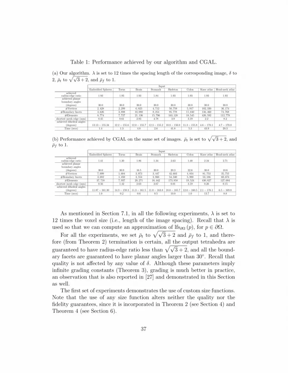
Table 1: Performance achieved by our algorithm and CGAL.
(a) Our algorithm. λ is set to 12 times the spacing length of the corresponding image, δ to
2, ρt to√√
3 + 2, and ρf to 1.
InputEmbedded Spheres Torus Brain Stomach Skeleton Colon Knee atlas Head-neck atlas
achievedradius-edge ratio 1.93 1.93 1.93 1.84 1.93 1.93 1.93 1.93achieved planarboundary angles
(degrees) 30.0 30.0 30.0 30.0 30.0 30.0 30.0 30.0#Vertices 2, 428 2, 299 6, 023 4, 712 50, 759 5, 917 102, 330 36, 174
#Boundary facets 3, 626 3, 898 10, 080 8, 254 95, 778 11, 040 146, 460 74, 768#Elements 8, 774 7, 727 21, 136 15, 796 163, 120 18, 545 426, 592 112, 778
shortest mesh edge (mm) 0.45 0.61 2.83 4.78 3.9 3.19 2.2 8.2achieved dihedral angles
(degrees) 13.13− 155.34 12.2− 155.6 12.0− 155.7 12.3− 155.2 10.8− 156.0 11.3− 155.8 4.6− 170.1 4.7− 170.0Time (secs) 1.4 1.3 4.8 2.6 41.8 5.3 43.9 20.3
(b) Performance achieved by CGAL on the same set of images. ρt is set to√√
3 + 2, andρf to 1.
InputEmbedded Spheres Torus Brain Stomach Skeleton Colon Knee atlas Head-neck atlas
achievedradius-edge ratio 1.41 1.30 1.86 1.34 2.63 1.40 2.34 2.71achieved planarboundary angles
(degrees) 30.0 30.0 16.5 30.0 20.3 22.6 30.0 10.6#Vertices 7, 099 1, 684 3, 973 3, 447 42, 603 4, 834 81, 753 35, 755
#Boundary facets 3, 682 1, 450 2, 554 2, 866 54, 340 5, 980 53, 186 60, 674#Elements 37, 718 7, 937 20, 271 16, 442 173, 858 19, 524 430, 827 127, 684
shortest mesh edge (mm) 0.56 1.42 2.63 3.67 0.01 3.19 0.26 0.15achieved dihedral angles
(degrees) 11.87− 161.30 14.3− 159.3 11.3− 161.5 11.0− 163.8 10.0− 165.7 12.0− 160.5 2.1− 176.1 6.5− 169.8Time (secs) 1.0 0.2 0.6 0.5 10.0 1.0 13.7 8.8
As mentioned in Section 7.1, in all the following experiments, λ is set to12 times the voxel size (i.e., length of the image spacing). Recall that λ isused so that we can compute an approximation of lfs∂Ω (p), for p ∈ ∂Ω.
For all the experiments, we set ρt to√√
3 + 2 and ρf to 1, and there-fore (from Theorem 2) termination is certain, all the output tetrahedra are
guaranteed to have radius-edge ratio less than√√
3 + 2, and all the bound-ary facets are guaranteed to have planar angles larger than 30. Recall thatquality is not affected by any value of δ. Although these parameters implyinfinite grading constants (Theorem 3), grading is much better in practice,an observation that is also reported in [27] and demonstrated in this Sectionas well.
The first set of experiments demonstrates the use of custom size functions.Note that the use of any size function alters neither the quality nor thefidelity guarantees, since it is incorporated in Theorem 2 (see Section 4) andTheorem 4 (see Section 6).
37

Table 2: Information about the input images.
Image Resolution Spacing (mm3) Tissues
Single Sphere 416× 416× 416 0.04× 0.04× 0.04 1Embedded Spheres 634× 416× 416 0.04× 0.04× 0.04 3
Torus 147× 147× 67 0.25× 0.25× 0.25 1Brain 316× 316× 188 0.93× 0.93× 1.5 1
Stomach 140× 186× 86 0.96× 0.96× 2.4 1Skeleton 359× 265× 218 0.96× 0.96× 2.4 1Colon 296× 167× 117 0.96× 0.96× 1.8 1
Knee atlas 413× 400× 116 0.27× 0.27× 1 49Head-neck atlas 241× 216× 228 0.97× 0.97× 1.4 60
We synthetically created the image of a sphere of radius 10mm and center(0, 0, 0). See Table 2 for information about this image. We ran our algorithmon the sphere image three times, each of which with a different size function:sf1 (·) , sf2 (·) , and sf3 (·). sf1 (·) restricts the radii of the elements to be smallerthan 5mm, while sf2 (·) restricts the radii of the elements to be smaller than1mm. sf3 (·) is a non-uniform size function. Specifically, it behaves as sf1 (·)for z ≥ 0 and as sf2 (·) for the other part of the sphere.
Figure 7 depicts the results. In all these three experiments, the achieved
radius-edge ratio is less than√√
3 + 2, and the planar angles are largerthan 30, as theory dictates. Moreover, the dihedral angles of the outputtetrahedra are between 12.9 and 155.8.
Observe that although parameters δ and λ (the ones directly responsiblefor the sampling density) are fixed for all three runs, the sample densityvaries. In fact, small size functions (i.e., size functions that take low values)make the boundary vertices denser (compare Figure 7a and Figure 7b forexample). Figure 7c shows better exactly that: the surface is sampled morewhere the size function takes low values, and less otherwise. This indirecteffect is expected and it is due to R3. Because of a small size function,more free vertices are inserter close to the surface. This, in turn, is likely toinvalidate more restricted facets; that is, more restricted facets will not havetheir vertices on the surface, and thus, R3 is triggered dictating the insertionof more feature vertices to protect the restricted facets.
The next set of experiments shows the output of our method on difficultgeometries both manifold and non manifold. Although the fidelity guarantees
38

(a) embedded spheres
(b) torus
Figure 8: The final meshes produced by our algorithm for the embeddedspheres and the torus. The first mesh of each row illustrates the whole meshand the second a cross-section of it.
about the topology of the output mesh are proved only for manifold domains,in this Section we show that our method behaves fairly well for non-manifoldcases (see Figure 11 for example) as well.
The first couple of images are the embedded spheres and a torus we syn-thetically created. The third is an MRI brain image obtained from HuashanHospital2. The next three images are CT segmented scans of a skeleton,a colon, and a stomach, obtained from IRCAD Laparoscopic Center3. Thelast two images are the MRI knee atlas [43] and the CT head-neck [44] atlasobtained from the Surgical Planning Laboratory of Brigham and Women’s
2Huashan Hospital, 12 Wulumuqi Zhong Lu, Shanghai, China.3http://www.ircad.fr/
39

(a) brain
(b) stomach
Figure 9: The final meshes produced by our algorithm for the brain and thestomach.
Hospital4. Information about the input images is shown in Table 2. Fig-ure 8, Figure 9, Figure 10, and Figure 11 show the meshes produced by ouralgorithm on these input images.
Table 1a reports some statistics for the meshes generated by our algo-rithm. The observed largest radius-edge ratio in all the meshes is no more
than√√
3 + 2 and the observed planar angles of the boundary facets in allmeshes is no smaller than 30 corroborating in this way the theory.
Also, for the meshes of Figure 8, Figure 9, Figure 10, and Figure 11, noticethat: (a) the interior of the object (i.e. the part away from the surface) ismeshed with fewer and bigger elements (volume grading), and (b) in mostcases, more and smaller boundary triangles mesh parts of the surface closeto the medial axis (surface grading). Graded meshes greatly reduce the total
4http://www.spl.harvard.edu/
40
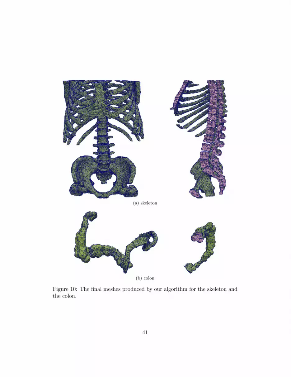
(a) skeleton
(b) colon
Figure 10: The final meshes produced by our algorithm for the skeleton andthe colon.
41

(a) knee atlas
(b) head-neck atlas
Figure 11: The final meshes produced by our algorithm for the multi-tissueknee and head-neck atlases.
number of elements, representing, at the same time, difficult geometries (i.e.,geometries with high curvature and/or non-manifold parts) accurately.
For comparison, Table 1b shows the meshes generated by CGAL [32], thestate of the art mesh generation tool we are aware of, able to operate directlyon images as well. We set the quality parameters to the same values with theones used in our algorithm. Note, however, that CGAL does not offer surfacegrading according to the local feature size. Nevertheless, we were able to setan upper limit on the radii of all the tetrahedra, so that the resulting mesheshave similar number of elements to the meshes produced by our algorithm.
Indeed, observe that both Table 1a and Table 1b report similar mesh
42

sizes on the same input image, with one exception: the mesh size on theEmbedded Spheres generated by CGAL is more than 4 times larger than theone generated by our method. The reason for this mismatch is the fact thatCGAL found it difficult to recover the red ball (see Figure 8a) with a smallnumber of elements. We had to considerably increase the size of the wholemesh so that CGAL could represent both connected components.
Table 1a and Table 1b suggest that the quality achieved by our method iscomparable to CGAL’s. The execution time of our method is much higher,but this is expected since the surface grading offered by our algorithm neces-sitates the computation of the poles and the maintenance of a second mesh,slowing down the overall meshing time. Improving the speed of our algorithmis outside the scope of this paper and is left for future work.
9. Conclusions
In this paper, we presented a 3D Delaunay refinement image-to-meshconversion algorithm that operates directly on segmented images. It is ableto create an appropriate sample set on the object’s surface, and to mesh thevolume and the surface at the same time. This flexibility (besides the factthat it solves three distinct problems, that is, sampling, surface recovery, andvolume meshing) results in a generally lower number of vertices than in thecase where the surface is meshed without considering the rules of quality.For instance, the insertion of points that improve the quality might help thedensity requirement at the same time.
Apart from the fidelity guarantees we give (namely, that the mesh bound-ary is a good geometric and topological approximation of the object’s sur-face), our algorithm provably achieves very low radius-edge ratio withoutsacrificing fidelity. The planar angles of the boundary facets are also guar-anteed to be larger than 30. Moreover, by slightly relaxing the qualityguarantees, our algorithm provably exhibits good grading.
Experimental evaluation on various images shows that the final meshesare free of slivers and exhibit both volume and (in most cases) surface grading,a fact that greatly reduces the size of the mesh making the subsequent FEManalysis [40, 41, 45] faster. Lastly, demonstration of the use of custom sizefunctions shows that our algorithm allows for additional flexibility to meetuser-defined mesh density.
43
Acknowledgments
The authors are deeply grateful to the reviewers for improving the manu-script with their constructive suggestions and comments. This work is sup-ported in part by NSF grants: CCF-1139864, CCF-1136538, and CSI-1136536and by the John Simon Guggenheim Foundation and the Richard T. ChengEndowment.
References
[1] J. R. Shewchuk, Tetrahedral mesh generation by Delaunay refinement,in: Proceedings of the 14th ACM Symposium on Computational Geom-etry, ACM, Minneapolis, MN, 1998, pp. 86–95.
[2] A. Chernikov, N. Chrisochoides, Three-Dimensional Semi-GeneralizedPoint Placement Method for Delaunay Mesh Refinement, in: Proceed-ings of the 16th International Meshing Roundtable, Elsevier, Seattle,WA, 2007, pp. 25–44.
[3] S. Oudot, L. Rineau, M. Yvinec, Meshing volumes bounded by smoothsurfaces, in: Proceedings of the International Meshing Roundtable,Springer-Verlag, 2005, pp. 203–219.
[4] L. Rineau, M. Yvinec, Meshing 3D domains bounded by piece-wise smooth surfaces, in: Proceedings of the International MeshingRoundtable, pp. 443–460.
[5] D. Boltcheva, M. Yvinec, J.-D. Boissonnat, Mesh Generation from 3DMulti-material Images, in: Medical Image Computing and Computer-Assisted Intervention, Springer, 2009, pp. 283–290.
[6] J.-P. Pons, F. Segonne, J.-D. Boissonnat, L. Rineau, M. Yvinec,R. Keriven, High-Quality Consistent Meshing of Multi-label Datasets,in: Information Processing in Medical Imaging, Springer Berlin Heidel-berg, 2007, pp. 198–210.
[7] L. P. Chew, Guaranteed-quality Delaunay meshing in 3D, in: Proceed-ings of the 13th ACM Symposium on Computational Geometry, Nice,France, pp. 391–393.
44
[8] S.-W. Cheng, T. K. Dey, H. Edelsbrunner, M. A. Facello, S.-H. Teng,Sliver exudation, Journal of the ACM 47 (2000) 883–904.
[9] P.-L. George, H. Borouchaki, Delaunay triangulation and meshing, Ap-plication to finite elements, HERMES, 1998.
[10] H. Si, Constrained Delaunay tetrahedral mesh generation and refine-ment, Finite Elements in Analysis and Design 46 (2010) 33–46.
[11] F. Labelle, J. R. Shewchuk, Isosurface stuffing: fast tetrahedral mesheswith good dihedral angles, ACM Transactions on Graphics 26 (2007)57.1–57.10.
[12] X.-Y. Li, S.-H. Teng, Generating Well-Shaped Delaunay meshed in3D, in: Proceedings of the 12th annual ACM-SIAM Symposium onDiscrete Algorithms, Society for Industrial and Applied Mathematics,Philadelphia, PA, USA, 2001, pp. 28–37.
[13] G. L. Miller, D. Talmor, S.-H. Teng, N. Walkington, A Delaunay basednumerical method for three dimensions: generation, formulation, andpartition, in: Proceedings of the 27th Annu. ACM Sympos. TheoryComput, ACM, 1995, pp. 683–692.
[14] L. P. Chew, Guaranteed-quality mesh generation for curved surfaces, in:Proceedings of the 9th ACM Symposium on Computational Geometry,San Diego, CA, pp. 274–280.
[15] N. Amenta, S. Choi, T. K. Dey, N. Leekha, A Simple Algorithm forHomeomorphic Surface Reconstruction, International Journal of Com-putational Geometry and Applications 12 (2002) 125–141.
[16] Jane Tournois, Rahul Srinivasan, Pierre Alliez, Perturbing Slivers in3D Delaunay Meshes, in: Proceedings of the 18th International MeshingRoundtable, Sandia Labs, Salt Lake City, Utah, USA, pp. 157–173.
[17] N. Amenta, M. Bern, Surface reconstruction by Voronoi filtering, in:SCG ’98: Proceedings of the fourteenth annual symposium on Compu-tational geometry, ACM, New York, NY, USA, 1998, pp. 39–48.
[18] N. Amenta, S. Choi, R. K. Kolluri, The power crust, in: Proceedingsof the sixth ACM symposium on Solid modeling and applications, SMA’01, ACM, New York, NY, USA, 2001, pp. 249–266.
45

[19] J.-D. Boissonnat, S. Oudot, Provably good sampling and meshing ofsurfaces, Graphical Models 67 (2005) 405–451.
[20] W. E. Lorensen, H. E. Cline, Marching cubes: A high resolution 3D sur-face construction algorithm, SIGGRAPH Computer Graphics 21 (1987)163–169.
[21] N. Molino, R. Bridson, J. Teran, R. Fedkiw, A crystalline, red greenstrategy for meshing highly deformable objects with tetrahedra, in: Pro-ceedings of the 12th International Meshing Roundtable, Sandia NationalLaboratories, 2003, pp. 103–114.
[22] A. Chernikov, N. Chrisochoides, Tetrahedral image-to-mesh conversionfor biomedical applications, in: ACM Conference on Bioinformatics,Computational Biology and Biomedicine, Chicago, IL, pp. 125–134.
[23] P. Alliez, D. Cohen-Steiner, M. Yvinec, M. Desbrun, Variational tetra-hedral meshing, ACM Trans. Graph. 24 (2005) 617–625.
[24] B. M. Klingner, J. R. Shewchuk, Aggressive tetrahedral mesh im-provement, in: Proceedings of the International Meshing Roundtable,Springer, 2007, pp. 3–23.
[25] L. A. Freitag, C. Ollivier-Gooch, Tetrahedral mesh improvement usingswapping and smoothing, International Journal for Numerical Methodsin Engineering 40 (1997) 3979–4002.
[26] H. Blum, A Transformation for Extracting New Descriptors of Shape,in: W. Wathen-Dunn (Ed.), Models for the Perception of Speech andVisual Form, MIT Press, Cambridge, 1967, pp. 362–380.
[27] J. R. Shewchuk, Delaunay refinement algorithms for triangular meshgeneration, Computational Geometry: Theory and Applications 22(2002) 21–74.
[28] S. A. Mitchell, Cardinality bounds for triangulations with boundedminimum angle, in: CCCG, pp. 326–331.
[29] G. L. Miller, D. Talmor, S.-H. Teng, Data generation for geometricalgorithms on non-uniform distributions, Int. J. Comput. GeometryAppl. 9 (1999) 577–598.
46

[30] ITK, Insight Segmentation and Registration Toolkit, http://www.itk.org, v4.1.0.
[31] C. R. Maurer, Q. Rensheng, V. Raghavan, A linear time algorithm forcomputing exact euclidean distance transforms of binary images in arbi-trary dimensions, IEEE Transactions on Pattern Analysis and MachineIntelligence 25 (2003) 265 – 270.
[32] Cgal, Computational Geometry Algorithms Library, http://www.
cgal.org, v4.0.
[33] T. K. Dey, W. Zhao, Approximate medial axis as a voronoi subcomplex,Computer-Aided Design 36 (2004) 195–202.
[34] P. Giblin, B. B. Kimia, A formal classification of 3D medial axis pointsand their local geometry, IEEE Transactions on Pattern Analysis andMachine Intelligence 26 (2004) 238–251.
[35] D. Coeurjolly, A. Montanvert, Optimal separable algorithms to computethe reverse euclidean distance transformation and discrete medial axis inarbitrary dimension, IEEE Trans. Pattern Anal. Mach. Intell. 29 (2007)437–448.
[36] F. Chazal, A. Lieutier, Stability and homotopy of a subset of the medialaxis, in: Proceedings of the ninth ACM symposium on Solid model-ing and applications, SM ’04, Eurographics Association, Aire-la-Ville,Switzerland, Switzerland, 2004, pp. 243–248.
[37] H. Edelsbrunner, D. Guoy, An experimental study of sliver exudation,Engineering with Computers 18 (2002) 229–240.
[38] A. Liu, B. Joe, On the shape of tetrahedra from bisection, Math.Comput. 63 (1994) 141–154.
[39] A. H. Squillacote, ParaView Guide, A Parallel Visualization Applica-tion, Kitware Inc., 2008.
[40] M. A. Audette, H. Delingette, A. Fuchs, O. Burgert, K. Chinzei, A topo-logically faithful, tissue-guided, spatially varying meshing strategy forcomputing patient-specific head models for endoscopic pituitary surgerysimulation, Computer Aided Surgery 12 (2007) 43–52.
47

[41] M. Audette, M. Miga, J. Nemes, K. Chinzei, T. Peters, A Reviewof Biomechanical Modeling of the Brain for Intrasurgical DisplacementEstimation and Medical Simulation, Biomechanical Systems, GeneralAnatomy (2007) 83–112.
[42] P. Foteinos, Y. Liu, A. Chernikov, N. Chrisochoides, An Evaluationof Tetrahedral Mesh Generation for Non-Rigid Registration of BrainMRI, in: Computational Biomechanics for Medicine V, 13th Interna-tional Conference on Medical Image Computing and Computer AssistedIntervention (MICCAI) Workshop, Springer, 2010, pp. 126–137.
[43] J. Richolt, M. Jakab, R. Kikinis, SPL Knee Atlas (2011). Available at:http://www.spl.harvard.edu/publications/item/view/1953.
[44] M. Jakab, R. Kikinis, Head and neck atlas (2012). Available at: http:
//www.spl.harvard.edu/publications/item/view/2271.
[45] O. Clatz, H. Delingette, I.-F. Talos, A. J. Golby, R. Kikinis, F. Jolesz,N. Ayache, S. Warfield, Robust non-rigid registration to capture brainshift from intra-operative MRI, IEEE Transactions on Medical Imaging24 (2005) 1417–1427.
48