This is an Accepted Manuscript, which has been through the Royal Society of Chemistry peer review process and has been accepted for publication.

Accepted Manuscripts are published online shortly after acceptance, before technical editing, formatting and proof reading. Using this free service, authors can make their results available to the community, in citable form, before we publish the edited article. We will replace this Accepted Manuscript with the edited and formatted Advance Article as soon as it is available.

You can find more information about Accepted Manuscripts in the Information for Authors.

Please note that technical editing may introduce minor changes to the text and/or graphics, which may alter content. The journal’s standard Terms & Conditions and the Ethical guidelines still apply. In no event shall the Royal Society of Chemistry be held responsible for any errors or omissions in this Accepted Manuscript or any consequences arising from the use of any information it contains.

Accepted Manuscript

www.rsc.org/pccp

PCCP

Anomalous diffusion models and their properties: non-stationarity,non-ergodicity, and ageing at the centenary of single particle tracking

Ralf Metzler,∗a,b Jae-Hyung Jeon,b,c, Andrey G. Cherstvy,a and Eli Barkaid

Received Xth XXXXXXXXXX 20XX, Accepted Xth XXXXXXXXX 20XXFirst published on the web Xth XXXXXXXXXX 200XDOI: 10.1039/b000000x

Abstract

Modern microscopic techniques following the stochastic mo-tion of labelled tracer particles have uncovered significant de-viations from the laws of Brownian motion in a variety ofanimate and inanimate systems. Such anomalous diffusioncan have different physical origins, which can be identifiedfrom careful data analysis. In particular, single particle track-ing provides the entire trajectory of the traced particle, whichallows one to evaluate different observables to quantify thedynamics of the system under observation. We here providean extensive overview over different popular anomalous diffu-sion models and their properties. We pay special attention totheir ergodic properties, highlighting the fact that in several ofthese models the long time averaged mean squared displace-ment shows a distinct disparity to the regular, ensemble aver-aged mean squared displacement. In these cases, data obtainedfrom time averages cannot be interpreted by the standard the-oretical results for the ensemble averages. Here we thereforeprovide a comparison of the main properties of the time aver-aged mean squared displacement and its statistical behaviourin terms of the scatter of the amplitudes between the timeaverages obtained from different trajectories. We especiallydemonstrate how anomalous dynamics may be identified forsystems, which, on first sight, appear Brownian. Moreover,we discuss the ergodicity breaking parameters for the differ-ent anomalous stochastic processes and showcase the physi-cal origins for the various behaviours. This Perspective is in-tended as a guidebook for both experimentalists and theoristsworking on systems, that exhibit anomalous diffusion.

a Institute of Physics and Astronomy, University of Potsdam, Potsdam-Golm,Germany; E-mail: rmetzler@uni-potsdam.deb Physics Department, Tampere University of Technology, Tampere, Finlandc Korean Institute for Advanced Study (KIAS), Seoul, Republik of Koread Physics Department and Institute of Nanotechnology and Advanced Mate-rials, Bar-Ilan University, Ramat Gan, Israel

1 Introduction and historical perspective

It is possible that the movements to be discussed here areidentical with the so-called “Brownian molecular motion”;however, the information available to me regarding the lat-ter is so lacking in precision, that I can form no judgment inthe matter. This statement is part of the introduction of Al-bert Einstein’s first and seminal 1905 paper on the theory ofdiffusion1. It refers to the observations reported by RobertBrown in 1828 of small granules (or Molecules, as I shallterm them) of 1

4000 th to 15000 th of an inch extracted from larger

pollen grains. Brown found these particles evidently in mo-tion2. Brown made meticulously sure that the motion he ob-served was not the effect of living matter, and he even stud-ied the motion of such Molecules as of a bruised fragment ofthe Sphinx2. In his second, 1906 paper Einstein then quotesthe experimental proof by Gouy3 that indeed the motion per-petuated by Robert Brown is caused by the irregular thermalmovements of the molecules of the liquid, and thus describedby Einstein’s theory1. As remarked by Marian Smoluchowskiin his equally seminal 1906 article4, Einstein reinvigorated theinterest in Brownian motion. Since then, the interest in themolecular phenomenon of diffusion is unbroken.

Considering the local concentration difference and thecounteracting flux of microscopic particles with a typicalmean free path, Einstein derived the diffusion equation1∗

∂∂ t

P(x, t) = K1∂ 2

∂x2 P(x, t) (1)

with the coefficient of diffusion K1 for the probability densityfunction (PDF) P(x, t) to find the particle under observationat position x at time t. This equation is indeed equivalent toFick’s second law for the concentration of a chemical sub-stance originally presented by Adolf Fick from a combinationof the continuity equation and the constitutive equation (Fick’s

∗For convenience, we express mathematical formula in one dimension.

1–40 | 1

Page 1 of 40 Physical Chemistry Chemical Physics

Phy

sica

lChe

mis

try

Che

mic

alP

hysi

csA

ccep

ted

Man

uscr

ipt

first law)5. If the particle is released at the origin at time t = 0in an unbounded space, the solution of the diffusion equation(1) is the normalised Gaussian PDF

P(x, t) =1√

4πK1texp

(− x2

4K1t

). (2)

Einstein remarks that this solution is that of the fortuitous er-ror, which was to be expected 1. From the PDF (2) we imme-diately obtain the variance

〈x2(t)〉=∫ ∞

−∞x2P(x, t)dx = 2K1t, (3)

the so-called mean squared displacement (MSD). From thedynamic equilibrium of suspended particles Einstein (and laterindependently Smoluchowski) derived the celebrated relation

K1 =kBTmη

=(R/NA)T

mη, (4)

between the diffusion coefficient, thermal energy kBT , themass m of the observed particle, and the friction coefficientη of unit 1/sec. In the second equality of Eq. (4) we replacedthe Boltzmann constant kB by the ratio of the gas constant R,quite precisely known at the time, and Avogadro’s number NA.

Yet another derivation of Brownian motion with the MSD(3) was published in 1908 by Paul Langevin using the conceptof a stochastic force. The Langevin equation combines New-ton’s second law with the white Gaussian noise ξ (t) of zeromean and autocorrelation function 〈ξ (t)ξ (t ′)〉 = 2K1δ (t −t ′)6,7. In its overdamped form relevant for the single particletracking experiments we will refer to below, it reads6,7

dx(t)dt

= ξ (t), (5)

The Langevin formalism represents a very intuitive physicalpicture for Brownian motion. From the Langevin equation (5)it is easy to get back to the MSD (3). Likely prompted bydiscussions with his friend Paul Langevin8, the fundamentalEinstein-Smoluchowski relation (4) led Jean Perrin at the Sor-bonne in Paris to conduct the first extensive and systematicmeasurement of the diffusion of single microscopic particlesto determine Avogadro’s number NA

9.†While Perrin was confined to short measured trajectories

and the need to use ensemble averages over not perfectly iden-tical particles, to our best knowledge it was Ivar Nordlund at

† For completeness we mention that theories of Brownian motion appeared ear-lier than Einstein’s works. In particular, the Dane Thorvald Thiele set up atheory for independent and normally distributed increments in his 1880 workon the least squares method 10. Louis Bachelier in Paris applied a stochasticprocess to model the dynamics of stock markets in 1900 11. Concurrently withEinstein, the Melbourne physicist William Sutherland followed similar linesas Einstein in his 1905 paper on diffusion 12.

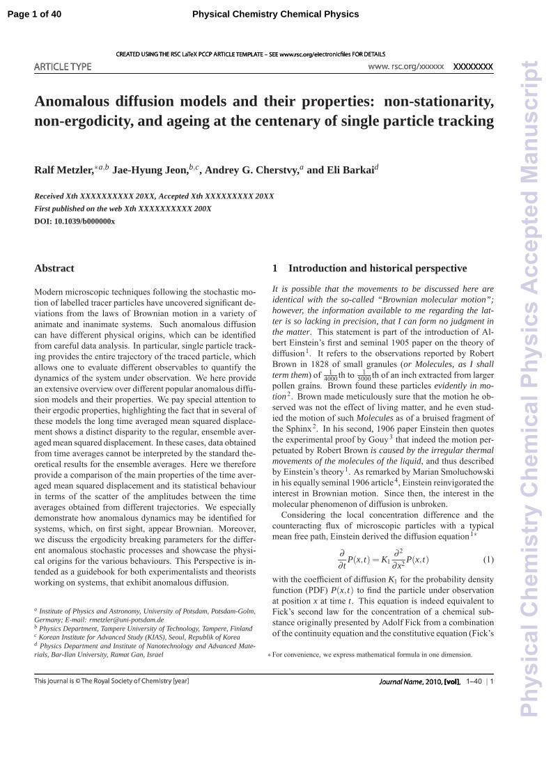
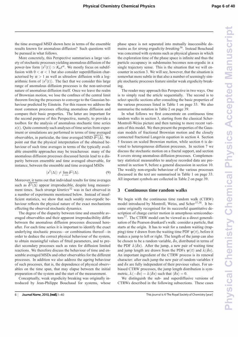
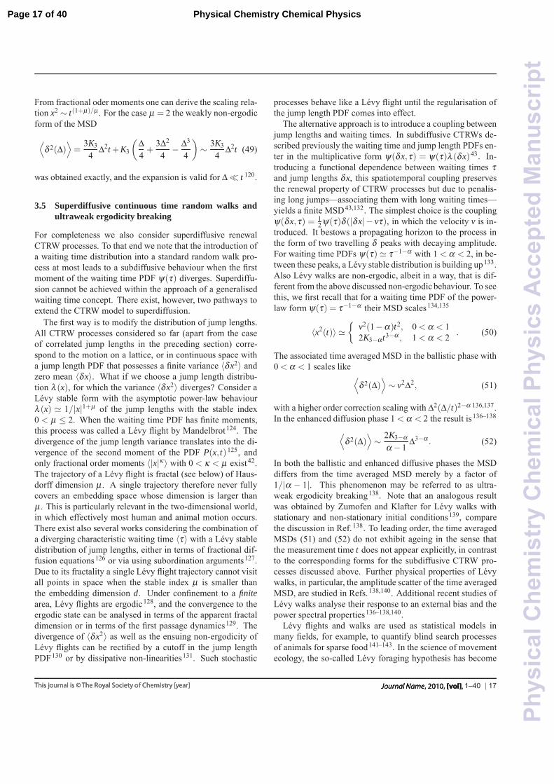
Fig. 1 Centennial single particle tracking experiments of IvarNordlund. Top: Nordlund’s experimental setup with the lightsource, an infrared absorbing water-filled cylinder, and theclock-controlled, electromagnetic shutter (on the table to the left)constituting a stroboscope. Mounted on the separate optical table onthe rack to the right, the object chamber with the mercury droplet, aswell as the objective and the camera are the heart of the experiment:the camera is connected to an electric motor moving thephotographic plate with constant velocity. Bottom: Example for thetime averaged mean squared displacement versus time (in seconds)from a single recorded mercury droplet. Images taken from Ref. 13.

2 | 1–40

Page 2 of 40Physical Chemistry Chemical Physics

Phy

sica

lChe

mis

try

Che

mic

alP

hysi

csA

ccep

ted

Man

uscr

ipt

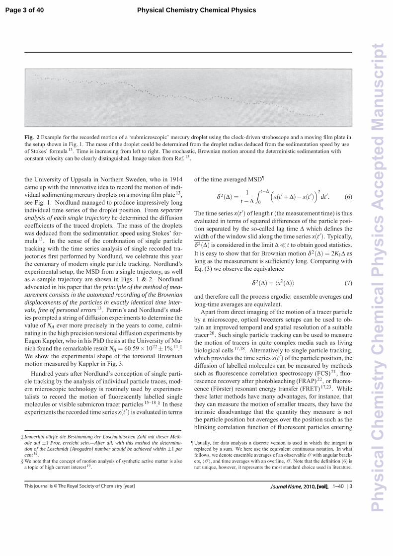
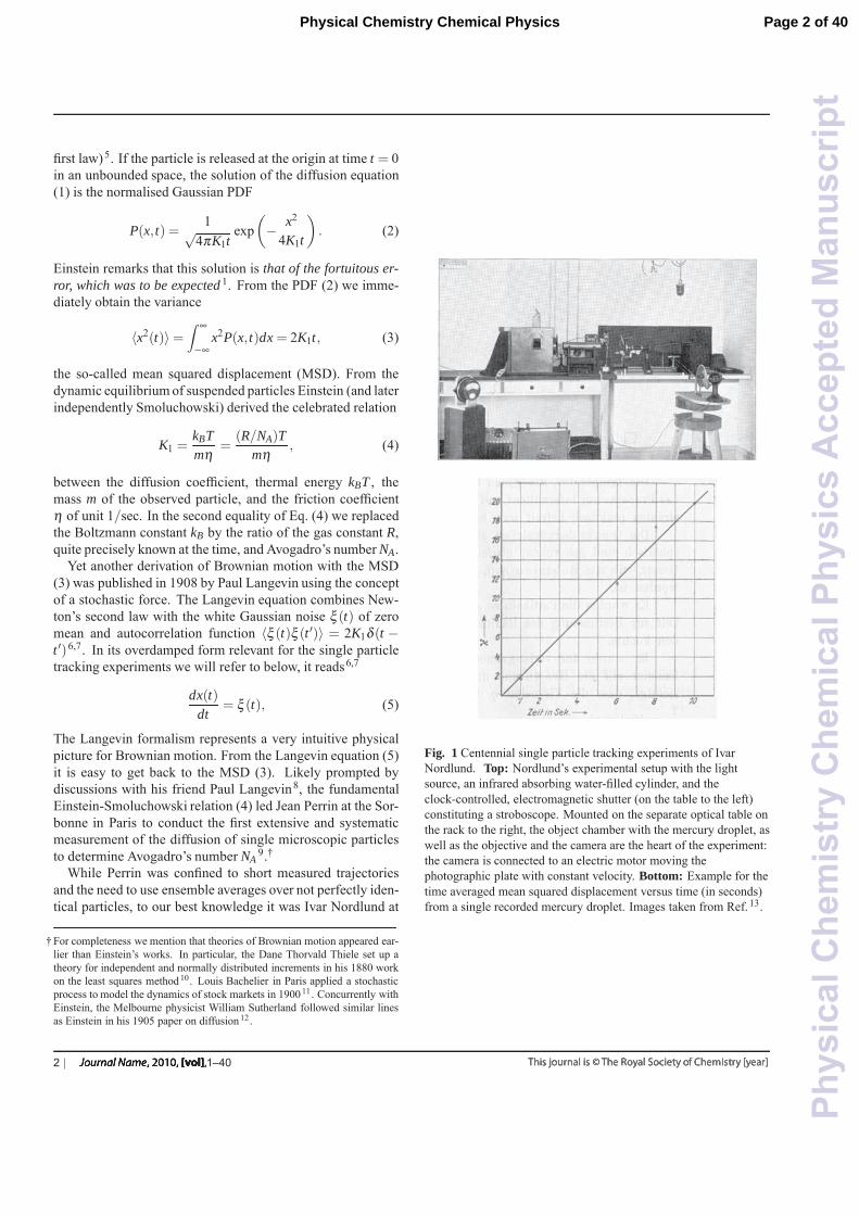
Fig. 2 Example for the recorded motion of a ‘submicroscopic’ mercury droplet using the clock-driven stroboscope and a moving film plate inthe setup shown in Fig. 1. The mass of the droplet could be determined from the droplet radius deduced from the sedimentation speed by useof Stokes’ formula13. Time is increasing from left to right. The stochastic, Brownian motion around the deterministic sedimentation withconstant velocity can be clearly distinguished. Image taken from Ref.13.

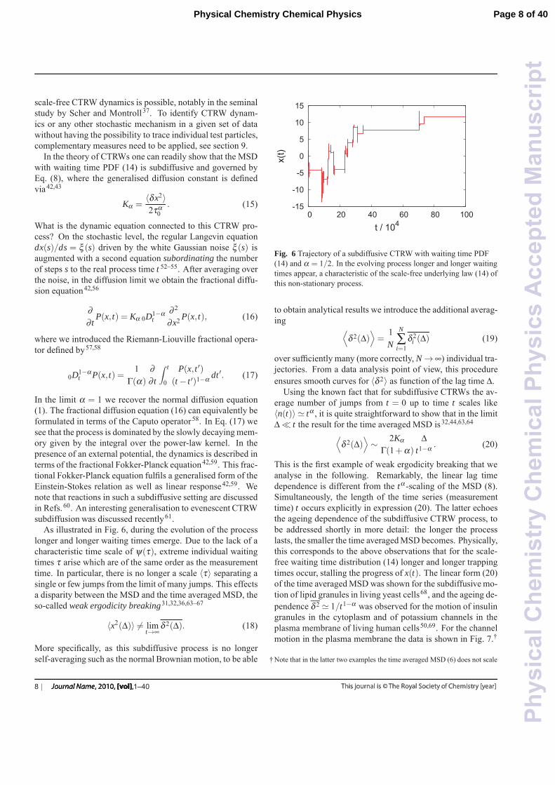
the University of Uppsala in Northern Sweden, who in 1914came up with the innovative idea to record the motion of indi-vidual sedimenting mercury droplets on a moving film plate13,see Fig. 1. Nordlund managed to produce impressively longindividual time series of the droplet position. From separateanalysis of each single trajectory he determined the diffusioncoefficients of the traced droplets. The mass of the dropletswas deduced from the sedimentation speed using Stokes’ for-mula13. In the sense of the combination of single particletracking with the time series analysis of single recorded tra-jectories first performed by Nordlund, we celebrate this yearthe centenary of modern single particle tracking. Nordlund’sexperimental setup, the MSD from a single trajectory, as wellas a sample trajectory are shown in Figs. 1 & 2. Nordlundadvocated in his paper that the principle of the method of mea-surement consists in the automated recording of the Browniandisplacements of the particles in exactly identical time inter-vals, free of personal errors13. Perrin’s and Nordlund’s stud-ies prompted a string of diffusion experiments to determine thevalue of NA ever more precisely in the years to come, culmi-nating in the high precision torsional diffusion experiments byEugen Kappler, who in his PhD thesis at the University of Mu-nich found the remarkable result NA = 60.59× 1022± 1%14.‡We show the experimental shape of the torsional Brownianmotion measured by Kappler in Fig. 3.

Hundred years after Nordlund’s conception of single parti-cle tracking by the analysis of individual particle traces, mod-ern microscopic technology is routinely used by experimen-talists to record the motion of fluorescently labelled singlemolecules or visible submicron tracer particles15–18.§ In theseexperiments the recorded time series x(t ′) is evaluated in terms

‡ Immerhin durfte die Bestimmung der Loschmidtschen Zahl mit dieser Meth-ode auf ±1 Proz. erreicht sein.—After all, with this method the determina-tion of the Loschmidt [Avogadro] number should be achieved within ±1 percent 14.

§ We note that the concept of motion analysis of synthetic active matter is alsoa topic of high current interest 19 .

of the time averaged MSD¶

δ 2(Δ) =1

t −Δ

∫ t−Δ

0

(x(t ′+Δ)− x(t ′)

)2dt ′. (6)

The time series x(t ′) of length t (the measurement time) is thusevaluated in terms of squared differences of the particle posi-tion separated by the so-called lag time Δ which defines thewidth of the window slid along the time series x(t ′). Typically,δ 2(Δ) is considered in the limit Δ� t to obtain good statistics.It is easy to show that for Brownian motion δ 2(Δ) = 2K1Δ aslong as the measurement is sufficiently long. Comparing withEq. (3) we observe the equivalence

δ 2(Δ) = 〈x2(Δ)〉 (7)

and therefore call the process ergodic: ensemble averages andlong-time averages are equivalent.

Apart from direct imaging of the motion of a tracer particleby a microscope, optical tweezers setups can be used to ob-tain an improved temporal and spatial resolution of a suitabletracer20. Such single particle tracking can be used to measurethe motion of tracers in quite complex media such as livingbiological cells17,18. Alternatively to single particle tracking,which provides the time series x(t ′) of the particle position, thediffusion of labelled molecules can be measured by methodssuch as fluorescence correlation spectroscopy (FCS)21, fluo-rescence recovery after photobleaching (FRAP)22, or fluores-cence (Forster) resonant energy transfer (FRET)17,23. Whilethese latter methods have many advantages, for instance, thatthey can measure the motion of smaller tracers, they have theintrinsic disadvantage that the quantity they measure is notthe particle position but averages over the position such as theblinking correlation function of fluorescent particles entering

¶ Usually, for data analysis a discrete version is used in which the integral isreplaced by a sum. We here use the equivalent continuous notation. In whatfollows, we denote ensemble averages of an observable O with angular brack-ets, 〈O〉, and time averages with an overline, O. Note that the definition (6) isnot unique, however, it represents the most standard choice used in literature.

1–40 | 3

Page 3 of 40 Physical Chemistry Chemical Physics

Phy

sica

lChe

mis

try

Che

mic

alP

hysi

csA

ccep

ted

Man

uscr

ipt

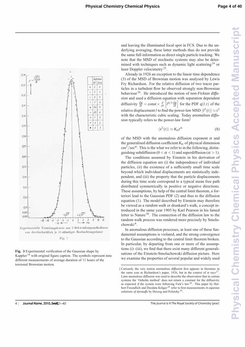
Fig. 3 Experimental verification of the Gaussian shape byKappler14 with original figure caption. The symbols represent ninedifferent measurements of average duration of 11 hours of thetorsional Brownian motion.

and leaving the illuminated focal spot in FCS. Due to the un-derlying averaging, these latter methods thus do not providethe same full information as direct single particle tracking. Wenote that the MSD of stochastic systems may also be deter-mined with techniques such as dynamic light scattering24 orlaser Doppler velocimetry25.

Already in 1926 an exception to the linear time dependence(3) of the MSD of Brownian motion was analysed by LewisFry Richardson. For the relative diffusion of two tracer par-ticles in a turbulent flow he observed strongly non-Brownianbehaviour26. He introduced the notion of non-Fickian diffu-sion and used a diffusion equation with separation dependentdiffusivity ∂q

∂ t = const× ∂∂ l

[l4/3 ∂q

∂ l

]for the PDF q(l, t) of the

relative displacement l to find the power-law MSD 〈l2(t)〉 � t3

with the characteristic cubic scaling. Today anomalous diffu-sion typically refers to the power-law form‖

〈x2(t)〉 � Kα tα (8)

of the MSD with the anomalous diffusion exponent α andthe generalised diffusion coefficient Kα of physical dimensioncm2/secα . This is the what we refer to in the following, distin-guishing subdiffusion (0< α < 1) and superdiffusion (α > 1).

The conditions assumed by Einstein in his derivation ofthe diffusion equation are (i) the independence of individualparticles, (ii) the existence of a sufficiently small time scalebeyond which individual displacements are statistically inde-pendent, and (iii) the property that the particle displacementsduring this time scale correspond to a typical mean free pathdistributed symmetrically in positive or negative directions.These assumptions, by help of the central limit theorem, a for-teriori lead to the Gaussian PDF (2) and thus to the diffusionequation (1). The model described by Einstein may thereforebe viewed as a random walk or drunkard’s walk, a concept in-troduced in the same year 1905 by Karl Pearson in his famedletter to Nature30. The connection of the diffusion law to therandom walk process was rendered more precisely by Smolu-chowski4.

In anomalous diffusion processes, at least one of these fun-damental assumptions is violated, and the strong convergenceto the Gaussian according to the central limit theorem broken.In particular, by departing from one or more of the assump-tions (i)–(iii), we find that there exist many different generali-sations of the Einstein-Smoluchowski diffusion picture. Herewe examine the properties of several popular and widely used

‖Curiously the very notion anomalous diffusion first appears in literature inthe same year as Richardson’s paper, 1926, but in the context of α rays 27.Later anomalous diffusion was used to describe the observation that in certainsystems the ‘Oeholm method’ does not return a constant for the diffusivityas expected if the system were following Fick’s law 28. This paper by Her-bert Freundlich and Deodata Kruger 28 refer to first measurements in aqueoussolutions of dyestuffs by Herzog and Polotzky 29.

4 | 1–40

Page 4 of 40Physical Chemistry Chemical Physics

Phy

sica

lChe

mis

try

Che

mic

alP

hysi

csA

ccep

ted

Man

uscr

ipt

0 0.5 1 1.5 1.5 2.5 3.5

log10Δ [sec] x [μm]

−3

−2

−1

0

log

10δ2

[μm

2]

1.5

3.0

y[μ

m]

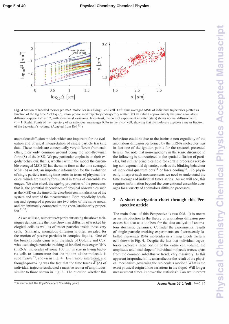
Fig. 4 Motion of labelled messenger RNA molecules in a living E.coli cell. Left: time averaged MSD of individual trajectories plotted asfunction of the lag time Δ of Eq. (6), show pronounced trajectory-to-trajectory scatter. Yet all exhibit approximately the same anomalousdiffusion exponent α ≈ 0.7, with some local variations. In contrast, the control experiment in water (stars) shows normal diffusion withα = 1. Right: Points of the trajectory of an individual messenger RNA in the E.coli cell, showing that the molecule explores a major fractionof the bacterium’s volume. (Adapted from Ref. 33.)

anomalous diffusion models which are important for the eval-uation and physical interpretation of single particle trackingdata. These models are conceptually very different from eachother, their only common ground being the non-Brownianform (8) of the MSD. We pay particular emphasis on their er-godic behaviour, that is, whether within the model the ensem-ble averaged MSD (8) has the same form as the time averagedMSD (6) or not, an important information for the evaluationof single particle tracking time series in terms of physical the-ories, which are usually formulated in terms of ensemble av-erages. We also check the ageing properties of the processes,that is, the potential dependence of physical observables suchas the MSD on the time difference between initialisation of thesystem and start of the measurement. Both ergodicity break-ing and ageing of a process are two sides of the same medaland are intimately connected to the (non-)stationarity proper-ties31,32.

As we will see, numerous experiments using the above tech-niques demonstrate the non-Brownian diffusion of tracked bi-ological cells as well as of tracer particles inside those verycells. Similarly, anomalous diffusion is often revealed forthe motion of passive particles in complex liquids. One ofthe breakthroughs came with the study of Golding and Cox,who used single particle tracking of labelled messenger RNA(mRNA) molecules of some 100 nm in size in living bacte-ria cells to demonstrate that the motion of the molecule issubdiffusive33, shown in Fig. 4. Even more interesting andthought-provoking was the fact that the time traces δ 2(Δ) ofindividual trajectories showed a massive scatter of amplitudes,similar to those shown in Fig. 8. The question whether this

behaviour could be due to the intrinsic non-ergodicity of theanomalous diffusion performed by the mRNA molecules wasin fact one of the ignition points for the research presentedherein. We note that non-ergodicity in the sense discussed inthe following is not restricted to the spatial diffusion of parti-cles, but similar principles hold for certain processes reveal-ing non-exponential dynamics, such as the blinking behaviourof individual quantum dots34 or laser cooling35. To physi-cally interpret such measurements we need to understand thetime averages of individual times series. As we will see, thisrequires information beyond the conventional ensemble aver-ages for a variety of anomalous diffusion processes.

2 A short navigation chart through this Per-spective article

The main focus of this Perspective is two-fold. It is meantas an introduction to the theory of anomalous diffusion pro-cesses but also as a toolbox for the data analysis of anoma-lous stochastic dynamics. Consider the experimental resultsof single particle tracking experiments on fluorescently la-belled messenger RNA molecules in a living E.coli bacteriacell shown in Fig. 4. Despite the fact that individual trajec-tories explore a large portion of the entire cell volume, theamplitude and local slope of individual molecule traces, apartfrom the common subdiffusive trend, vary massively. Is thisapparent irreproducibility an artefact or the result of the physi-cal mechanism governing the molecule’s motion? What is theexact physical origin of the variations in the slope? Will longermeasurement times improve the statistics? Can we interpret

1–40 | 5

Page 5 of 40 Physical Chemistry Chemical Physics

Phy

sica

lChe

mis

try

Che

mic

alP

hysi

csA

ccep

ted

Man

uscr

ipt

the time averaged MSD shown here in terms of the ensembleresults known for anomalous diffusion? Such questions willbe pursued in what follows.

More concretely, this Perspective summarises a large vari-ety of stochastic processes yielding anomalous diffusion of thepower-law form 〈x2(t)〉 � Kα tα . We mostly focus on subdif-fusion with 0 < α < 1 but also consider superdiffusion char-acterised by α > 1 as well as ultraslow diffusion with a log-arithmic form of 〈x2(t)〉. The fact that we consider this largerange of anomalous diffusion processes is the non-universalnature of anomalous diffusion itself. Once we leave the realmof Brownian motion, we lose the confines of the central limittheorem forcing the processes to converge to the Gaussian be-haviour predicted by Einstein. For this reason we address themost common processes effecting anomalous diffusion andcompare their basic properties. The latter are important forthe second purpose of this Perspective, namely, to provide atoolbox for the analysis of anomalous stochastic time seriesx(t). Quite commonly such analyses of time series from exper-iment or simulations are performed in terms of time averagedobservables, in particular, the time averaged MSD δ 2(Δ). Wepoint out that the physical interpretation of the obtained be-haviour of such time averages in terms of the typically avail-able ensemble approaches may be treacherous: many of theanomalous diffusion processes discussed herein lead to a dis-parity between ensemble and time averaged observable, forinstance, between the ensemble and time averaged MSDs

〈x2(Δ)〉 �= limt→∞

δ 2(Δ). (9)

Moreover, it turns out that individual results for time averagessuch as δ 2(Δ) appear irreproducible, despite long measure-ment times. Such strange kinetics32 was in fact observed ina number of experiments mentioned below. Instead of insuf-ficient statistics, we show that such weakly non-ergodic be-haviour reflects the physical nature of the exact mechanismseffecting the observed stochastic dynamics.

The degree of the disparity between time and ensemble av-eraged observables and their apparent irreproducibility differbetween the anomalous diffusion processes discussed here-after. For each time series it is important to identify the exactunderlying stochastic process—or combinations thereof—inorder to deduce the correct physical behaviour of the system,to obtain meaningful values of fitted parameters, and to pre-dict secondary processes such as rates for diffusion limitedreactions. We therefore discuss the behaviour of time and en-semble averaged MSDs and other observables for the differentprocesses. In addition we also address the ageing behaviourof such processes, that is, the dependence of physical observ-ables on the time span, that may elapse between the initialpreparation of the system and the start of the measurement.

Conceptually, weak ergodicity breaking was originally in-troduced by Jean-Philippe Bouchaud for systems, whose

phase space is not separated into mutually inaccessible do-mains as for strong ergodicity breaking36. Instead Bouchaudwas concerned with systems such as physical glasses in whichthe exploration time of the phase space is infinite and thus theparticle occupancy in subdomains becomes non-ergodic in asingle trajectory sense. This is the situation that we will en-counter in section 3. We will see, however, that the situation issomewhat more subtle in that also a number of seemingly sim-ple stochastic processes feature similar weak ergodicity break-ing.

The reader may approach this Perspective in two ways. Oneis to simply read the article sequentially. The second is toselect specific sections after consulting the basic properties ofthe various processes listed in Table 1 on page 33. We alsosummarise the notation in Table 2 on page 39.

In what follows we first concentrate on continuous timerandom walks in section 3, starting from the classical Scher-Montroll-Weiss picture and then turning to more recent vari-ants of this model. We then present the properties of the Gaus-sian models of fractional Brownian motion and the closelyconnected fractional Langevin equation in section 4. Section5 focuses on scaled Brownian motion, while section 6 is de-voted to heterogeneous diffusion processes. In section 7 wediscuss the stochastic motion on a fractal support, and section8 covers strong anomalous diffusion processes. Complemen-tary statistical measurables to analyse recorded data are pre-sented in section 9, before a general discussion in section 10.The weakly non-ergodic behaviour of the various processesdiscussed in the text are summarised in Table 1 on page 33.All important symbols are collected in Table 2 on page 39.

3 Continuous time random walks

We begin with the continuous time random walk (CTRW)model introduced by Montroll, Weiss, and Scher37,38. It be-came originally recognised for its successful quantitative de-scription of charge carrier motion in amorphous semiconduc-tors37. The CTRW model can be viewed as a direct generali-sation of the Pearson drunkard’s walk: consider a particle, thatstarts at the origin. It has to wait for a random waiting (trap-ping) time τ drawn from the waiting time PDF ψ(τ), before itmakes a jump to left or right. The length of the jump can alsobe chosen to be a random variable, δx, distributed in terms ofthe PDF λ (δx). After the jump, a new pair of waiting timeand jump length are drawn from the PDFs ψ(τ) and λ (δx).An important ingredient of the CTRW process is its renewalcharacter: after each jump the new pair of random variables τand δx are fully independent of their previous values. For un-biased CTRW processes, the jump length distribution is sym-metric, λ (−δx) = λ (δx) such that 〈δx〉= 0.

We distinguish the sub- and superdiffusive versions ofCTRWs described in the following subsections. These cases

6 | 1–40

Page 6 of 40Physical Chemistry Chemical Physics

Phy

sica

lChe

mis

try

Che

mic

alP

hysi

csA

ccep

ted

Man

uscr

ipt

arise depending on whether the characteristic waiting time

〈τ〉=∫ ∞

0τψ(τ)dτ (10)

and the variance of the jump length

〈δx2〉=∫ ∞

−∞(δx)2λ (δx)d(δx) (11)

are finite or infinite, respectively. In case of diverging mo-ments 〈τ〉 or 〈δx2〉 the anomalous character of the resultingstochastic process is effected due to the Levy-Khintchine gen-eralised central limit theorem (Levy statistics)39–41, accord-ing to which sums of independent and identically distributedrandom variables with diverging moments are stable distribu-tions, compare also section 8. Simply put, this means the oc-currence of power-law tails of the waiting time or jump lengthPDFs. In particular, we may find non-exponential relaxationpatterns and non-Gaussian spatial distributions42. Apart fromrenewal CTRW processes, in this section we also mention twonon-renewal versions of CTRWs.

Let us first briefly consider the case when both 〈τ〉 and〈δx2〉 are finite. In the diffusion limit this process corre-sponds to that of regular Brownian motion with MSD (3),i.e., α = 1 in Eq. (8), where the diffusion constant is de-fined as K1 = 〈δx2〉/(2〈τ〉) in the limiting sense of a randomwalk42,43. Note that apart from the finiteness of the moments〈τ〉 and 〈δx2〉 the details of the PDFs ψ(τ) and λ (δx) areirrelevant for the diffusive properties of the CTRW process.In this case of normal diffusion we also immediately evalu-ate the integrand in the time averaged MSD (6). Namely, weknow that as long as the lag time Δ is much larger than thecharacteristic time 〈τ〉 for a single jump, the average num-ber of jumps during this time span equals Δ/〈τ〉. Thus, thekernel [x(t ′ + Δ)− x(t ′)]2 in Eq. (6) on average is given by〈δx2〉Δ/〈τ〉. With the diffusion constant K1 = 〈δx2〉/(2〈τ〉),the result is

limt→∞

δ 2(Δ) = 2K1Δ. (12)

Identifying the lag time Δ with the regular time t in the MSD(8), we indeed find the equivalence

〈x2(Δ)〉= limt→∞

δ 2(Δ) (13)

between the MSD 〈x2〉 and the time averaged MSD δ 2 whichis expected in an ergodic system32,44–47.

3.1 Subdiffusive continuous time random walks

We first study the case when the jump lengths are suffi-ciently narrowly distributed such that 〈δx2〉 is finite. Forinstance, this could correspond to a Gaussian form for thePDF λ (δx) or the motion on a lattice of spacing a, with

101

102

103

104

0.1 1 10100

101

102

103

ψ(τ

) C

lust

ered

cha

nnel

s

ψ(τ

) Fr

ee c

hann

els

τ [sec]

τ-1.9

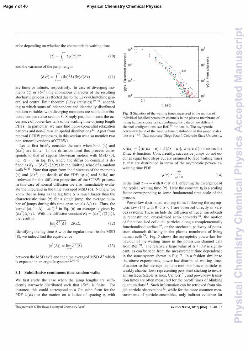
Fig. 5 Statistics of the waiting times measured in the motion ofindividual labelled potassium channels in the plasma membrane ofliving human kidney cells, combining the data of two differentchannel configurations, see Ref. 50 for details. The asymptoticpower-law trend of the waiting time distribution in this graph scaleslike � τ−1.9. Data courtesy Diego Krapf, Colorado State University.

λ (δx) = 12 [δ (δx− a) + δ (δx+ a)], where δ (·) denotes the

Dirac δ -function. Concurrently, successive jumps do not oc-cur at equal time steps but are assumed to face waiting timesτ , that are distributed in terms of the asymptotic power-lawwaiting time PDF

ψ(τ)� τα0

τ1+α (14)

in the limit τ → ∞ with 0 < α < 1, effecting the divergence ofthe typical waiting time 〈τ〉. Here the constant τ0 is a scalingfactor corresponding to some fundamental time scale of theprocess.

Power-law distributed waiting times following the asymp-totic law (14) with 0 < α < 1 are observed directly in vari-ous systems. These include the diffusion of tracer microbeadsin reconstituted, cross-linked actin networks48, the motionof functionalised colloidal particles along a complementarilyfunctionalised surface49, or the stochastic pathway of potas-sium channels diffusing in the plasma membrane of livinghuman cells50. Fig. 5 shows the asymptotic power-law be-haviour of the waiting times in the potassium channel datafrom Ref.50. The relatively large value of α ≈ 0.9 is signifi-cant, as can be seen from the measurement time dependencein the same system shown in Fig. 7. In a fashion similar tothe above experiments, power-law distributed waiting timescharacterise the interruption in the motion of tracer particles inweakly chaotic flows representing persistent sticking to invari-ant surfaces (stable islands, Cantori)51, and power-law transi-tion times are often measured for the on/off times of blinkingquantum dots34. Such information can be retrieved from sin-gle particle observations32, while for the more common mea-surements of particle ensembles, only indirect evidence for

1–40 | 7

Page 7 of 40 Physical Chemistry Chemical Physics

Phy

sica

lChe

mis

try

Che

mic

alP

hysi

csA

ccep

ted

Man

uscr

ipt

scale-free CTRW dynamics is possible, notably in the seminalstudy by Scher and Montroll37. To identify CTRW dynam-ics or any other stochastic mechanism in a given set of datawithout having the possibility to trace individual test particles,complementary measures need to be applied, see section 9.

In the theory of CTRWs one can readily show that the MSDwith waiting time PDF (14) is subdiffusive and governed byEq. (8), where the generalised diffusion constant is definedvia42,43

Kα =〈δx2〉2τα

0. (15)

What is the dynamic equation connected to this CTRW pro-cess? On the stochastic level, the regular Langevin equationdx(s)/ds = ξ (s) driven by the white Gaussian noise ξ (s) isaugmented with a second equation subordinating the numberof steps s to the real process time t 52–55. After averaging overthe noise, in the diffusion limit we obtain the fractional diffu-sion equation42,56

∂∂ t

P(x, t) = Kα 0D1−αt

∂ 2

∂x2 P(x, t), (16)

where we introduced the Riemann-Liouville fractional opera-tor defined by57,58

0D1−αt P(x, t) =

1Γ(α)

∂∂ t

∫ t

0

P(x, t ′)(t − t ′)1−α dt ′. (17)

In the limit α = 1 we recover the normal diffusion equation(1). The fractional diffusion equation (16) can equivalently beformulated in terms of the Caputo operator58. In Eq. (17) wesee that the process is dominated by the slowly decaying mem-ory given by the integral over the power-law kernel. In thepresence of an external potential, the dynamics is described interms of the fractional Fokker-Planck equation42,59. This frac-tional Fokker-Planck equation fulfils a generalised form of theEinstein-Stokes relation as well as linear response42,59. Wenote that reactions in such a subdiffusive setting are discussedin Refs.60. An interesting generalisation to evenescent CTRWsubdiffusion was discussed recently61.

As illustrated in Fig. 6, during the evolution of the processlonger and longer waiting times emerge. Due to the lack of acharacteristic time scale of ψ(τ), extreme individual waitingtimes τ arise which are of the same order as the measurementtime. In particular, there is no longer a scale 〈τ〉 separating asingle or few jumps from the limit of many jumps. This effectsa disparity between the MSD and the time averaged MSD, theso-called weak ergodicity breaking31,32,36,63–67

〈x2(Δ)〉 �= limt→∞

δ 2(Δ). (18)

More specifically, as this subdiffusive process is no longerself-averaging such as the normal Brownian motion, to be able

-15

-10

-5

0

5

10

15

0 20 40 60 80 100

x(t)

t / 104

Fig. 6 Trajectory of a subdiffusive CTRW with waiting time PDF(14) and α = 1/2. In the evolving process longer and longer waitingtimes appear, a characteristic of the scale-free underlying law (14) ofthis non-stationary process.

to obtain analytical results we introduce the additional averag-ing ⟨

δ 2(Δ)⟩=

1N

N

∑i=1

δ 2i (Δ) (19)

over sufficiently many (more correctly, N → ∞) individual tra-jectories. From a data analysis point of view, this procedureensures smooth curves for 〈δ 2〉 as function of the lag time Δ.

Using the known fact that for subdiffusive CTRWs the av-erage number of jumps from t = 0 up to time t scales like〈n(t)〉 � tα , it is quite straightforward to show that in the limitΔ � t the result for the time averaged MSD is32,44,63,64⟨

δ 2(Δ)⟩∼ 2Kα

Γ(1+α)

Δt1−α . (20)

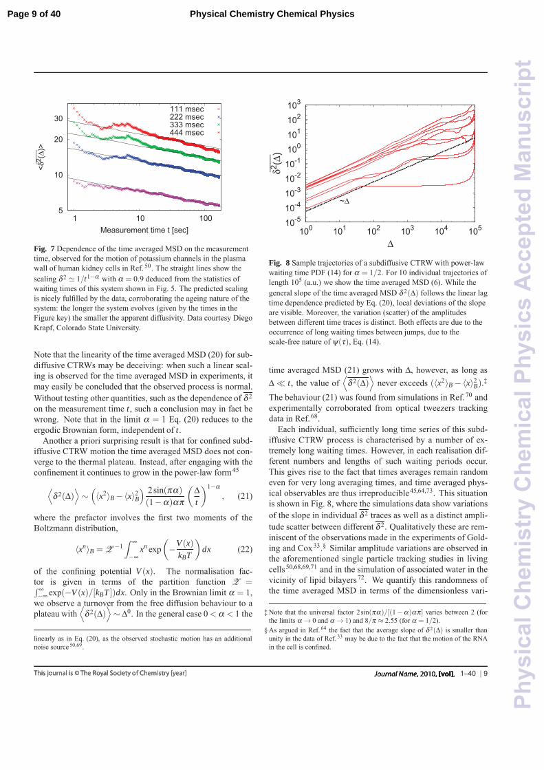
This is the first example of weak ergodicity breaking that weanalyse in the following. Remarkably, the linear lag timedependence is different from the tα -scaling of the MSD (8).Simultaneously, the length of the time series (measurementtime) t occurs explicitly in expression (20). The latter echoesthe ageing dependence of the subdiffusive CTRW process, tobe addressed shortly in more detail: the longer the processlasts, the smaller the time averaged MSD becomes. Physically,this corresponds to the above observations that for the scale-free waiting time distribution (14) longer and longer trappingtimes occur, stalling the progress of x(t). The linear form (20)of the time averaged MSD was shown for the subdiffusive mo-tion of lipid granules in living yeast cells68, and the ageing de-pendence δ 2 � 1/t1−α was observed for the motion of insulingranules in the cytoplasm and of potassium channels in theplasma membrane of living human cells50,69. For the channelmotion in the plasma membrane the data is shown in Fig. 7.†

† Note that in the latter two examples the time averaged MSD (6) does not scale

8 | 1–40

Page 8 of 40Physical Chemistry Chemical Physics

Phy

sica

lChe

mis

try

Che

mic

alP

hysi

csA

ccep

ted

Man

uscr

ipt

5

10

20

30

1 10 100

< ___

_δ2 (

Δ)>

Measurement time t [sec]

111 msec222 msec333 msec444 msec

Fig. 7 Dependence of the time averaged MSD on the measurementtime, observed for the motion of potassium channels in the plasmawall of human kidney cells in Ref. 50. The straight lines show thescaling δ 2 � 1/t1−α with α = 0.9 deduced from the statistics ofwaiting times of this system shown in Fig. 5. The predicted scalingis nicely fulfilled by the data, corroborating the ageing nature of thesystem: the longer the system evolves (given by the times in theFigure key) the smaller the apparent diffusivity. Data courtesy DiegoKrapf, Colorado State University.

Note that the linearity of the time averaged MSD (20) for sub-diffusive CTRWs may be deceiving: when such a linear scal-ing is observed for the time averaged MSD in experiments, itmay easily be concluded that the observed process is normal.Without testing other quantities, such as the dependence of δ 2

on the measurement time t, such a conclusion may in fact bewrong. Note that in the limit α = 1 Eq. (20) reduces to theergodic Brownian form, independent of t.

Another a priori surprising result is that for confined subd-iffusive CTRW motion the time averaged MSD does not con-verge to the thermal plateau. Instead, after engaging with theconfinement it continues to grow in the power-law form45

⟨δ 2(Δ)

⟩∼

(〈x2〉B −〈x〉2

B

) 2sin(πα)

(1−α)απ

(Δt

)1−α, (21)

where the prefactor involves the first two moments of theBoltzmann distribution,

〈xn〉B = Z−1

∫ ∞

−∞xn exp

(−V (x)

kBT

)dx (22)

of the confining potential V (x). The normalisation fac-tor is given in terms of the partition function Z =∫ ∞−∞ exp(−V (x)/[kBT ])dx. Only in the Brownian limit α = 1,

we observe a turnover from the free diffusion behaviour to aplateau with

⟨δ 2(Δ)

⟩∼ Δ0. In the general case 0 < α < 1 the

linearly as in Eq. (20), as the observed stochastic motion has an additionalnoise source 50,69.

10-510-410-310-210-1100101102103

100 101 102 103 104 105

___

_δ2 (

Δ)

Δ

~Δ

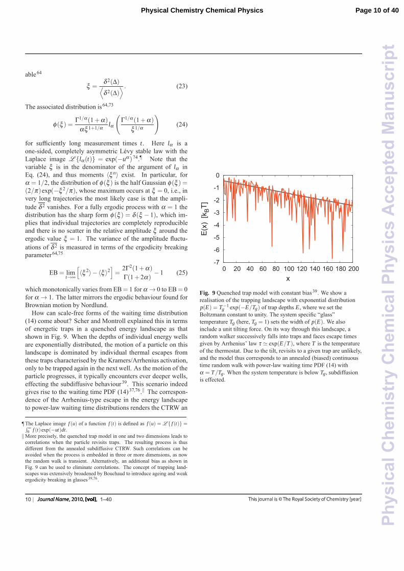
Fig. 8 Sample trajectories of a subdiffusive CTRW with power-lawwaiting time PDF (14) for α = 1/2. For 10 individual trajectories oflength 105 (a.u.) we show the time averaged MSD (6). While thegeneral slope of the time averaged MSD δ 2(Δ) follows the linear lagtime dependence predicted by Eq. (20), local deviations of the slopeare visible. Moreover, the variation (scatter) of the amplitudesbetween different time traces is distinct. Both effects are due to theoccurrence of long waiting times between jumps, due to thescale-free nature of ψ(τ), Eq. (14).

time averaged MSD (21) grows with Δ, however, as long asΔ � t, the value of

⟨δ 2(Δ)

⟩never exceeds (〈x2〉B −〈x〉2

B).‡

The behaviour (21) was found from simulations in Ref.70 andexperimentally corroborated from optical tweezers trackingdata in Ref.68.

Each individual, sufficiently long time series of this subd-iffusive CTRW process is characterised by a number of ex-tremely long waiting times. However, in each realisation dif-ferent numbers and lengths of such waiting periods occur.This gives rise to the fact that times averages remain randomeven for very long averaging times, and time averaged phys-ical observables are thus irreproducible45,64,73. This situationis shown in Fig. 8, where the simulations data show variationsof the slope in individual δ 2 traces as well as a distinct ampli-tude scatter between different δ 2. Qualitatively these are rem-iniscent of the observations made in the experiments of Gold-ing and Cox33.§ Similar amplitude variations are observed inthe aforementioned single particle tracking studies in livingcells50,68,69,71 and in the simulation of associated water in thevicinity of lipid bilayers72. We quantify this randomness ofthe time averaged MSD in terms of the dimensionless vari-

‡ Note that the universal factor 2sin(πα)/[(1−α)απ] varies between 2 (forthe limits α → 0 and α → 1) and 8/π ≈ 2.55 (for α = 1/2).

§ As argued in Ref. 64 the fact that the average slope of δ 2(Δ) is smaller thanunity in the data of Ref. 33 may be due to the fact that the motion of the RNAin the cell is confined.

1–40 | 9

Page 9 of 40 Physical Chemistry Chemical Physics

Phy

sica

lChe

mis

try

Che

mic

alP

hysi

csA

ccep

ted

Man

uscr

ipt

able64

ξ =δ 2(Δ)⟨δ 2(Δ)

⟩ . (23)

The associated distribution is64,73

φ(ξ ) =Γ1/α(1+α)

αξ 1+1/α lα

(Γ1/α(1+α)

ξ 1/α

)(24)

for sufficiently long measurement times t. Here lα is aone-sided, completely asymmetric Levy stable law with theLaplace image L {lα(t)} = exp(−uα)74.¶ Note that thevariable ξ is in the denominator of the argument of lα inEq. (24), and thus moments 〈ξ n〉 exist. In particular, forα = 1/2, the distribution of φ(ξ ) is the half Gaussian φ(ξ ) =(2/π)exp(−ξ 2/π), whose maximum occurs at ξ = 0, i.e., invery long trajectories the most likely case is that the ampli-tude δ 2 vanishes. For a fully ergodic process with α = 1 thedistribution has the sharp form φ(ξ ) = δ (ξ − 1), which im-plies that individual trajectories are completely reproducibleand there is no scatter in the relative amplitude ξ around theergodic value ξ = 1. The variance of the amplitude fluctu-ations of δ 2 is measured in terms of the ergodicity breakingparameter64,75

EB = limt→∞

[〈ξ 2〉− 〈ξ 〉2

]=

2Γ2(1+α)

Γ(1+ 2α)− 1 (25)

which monotonically varies from EB= 1 for α → 0 to EB = 0for α → 1. The latter mirrors the ergodic behaviour found forBrownian motion by Nordlund.

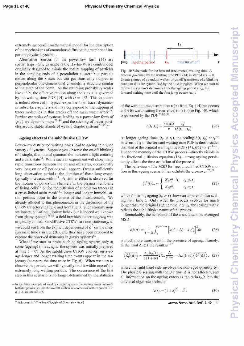
How can scale-free forms of the waiting time distribution(14) come about? Scher and Montroll explained this in termsof energetic traps in a quenched energy landscape as thatshown in Fig. 9. When the depths of individual energy wellsare exponentially distributed, the motion of a particle on thislandscape is dominated by individual thermal escapes fromthese traps characterised by the Kramers/Arrhenius activation,only to be trapped again in the next well. As the motion of theparticle progresses, it typically encounters ever deeper wells,effecting the subdiffusive behaviour39. This scenario indeedgives rise to the waiting time PDF (14)37,76.‖ The correspon-dence of the Arrhenius-type escape in the energy landscapeto power-law waiting time distributions renders the CTRW an

¶ The Laplace image f (u) of a function f (t) is defined as f (u) = L { f (t)} =∫ ∞0 f (t)exp(−ut)dt.

‖More precisely, the quenched trap model in one and two dimensions leads tocorrelations when the particle revisits traps. The resulting process is thusdifferent from the annealed subdiffusive CTRW. Such correlations can beavoided when the process is embedded in three or more dimensions, as nowthe random walk is transient. Alternatively, an additional bias as shown inFig. 9 can be used to eliminate correlations. The concept of trapping land-scapes was extensively broadened by Bouchaud to introduce ageing and weakergodicity breaking in glasses 39,76.

-7

-6

-5

-4

-3

-2

-1

0

0 20 40 60 80 100 120 140 160 180 200

E(x

) [k

BT]

x

Fig. 9 Quenched trap model with constant bias39. We show arealisation of the trapping landscape with exponential distributionp(E) = T−1

g exp(−E/Tg) of trap depths E, where we set theBoltzmann constant to unity. The system specific “glass”temperature Tg (here, Tg = 1) sets the width of p(E). We alsoinclude a unit tilting force. On its way through this landscape, arandom walker successively falls into traps and faces escape timesgiven by Arrhenius’ law τ � exp(E/T ), where T is the temperatureof the thermostat. Due to the tilt, revisits to a given trap are unlikely,and the model thus corresponds to an annealed (biased) continuoustime random walk with power-law waiting time PDF (14) withα = T/Tg. When the system temperature is below Tg, subdiffusionis effected.

10 | 1–40

Page 10 of 40Physical Chemistry Chemical Physics

Phy

sica

lChe

mis

try

Che

mic

alP

hysi

csA

ccep

ted

Man

uscr

ipt

extremely successful mathematical model for the descriptionof the mechanisms of anomalous diffusion in a number of im-portant physical systems.

Alternative sources for the power-law form (14) arespatial traps. One example is the Havlin-Weiss comb modeloriginally designed to mimic the spatial trapping of particlesin the dangling ends of a percolation cluster77: a particlemoves along the x axis but can get transiently trapped inperpendicular one-dimensional channels, a structure similarto the teeth of the comb. As the returning probability scaleslike t−1/2, the effective motion along the x axis is governedby the waiting time PDF (14) with α = 1/2. This exponentis indeed observed in typical experiments of tracer dynamicsin subsurface aquifers and may correspond to the trapping oftracer molecules in thin cracks off the main water artery78.Further examples of systems leading to a power-law form ofψ(τ) are dynamic maps79–84 and the sticking of tracer parti-cles around stable islands of weakly chaotic systems51,85.∗∗

Ageing effects of the subdiffusive CTRW

Power-law distributed waiting times lead to ageing in a widevariety of systems. Suppose you observe the on/off blinkingof a single, illuminated quantum dot between a light emittingand a dark state34. While such an experiment will show manyrapid transitions between the on and off states, occasionallyvery long on or off periods will appear. Over a sufficientlylong observation period t, the duration of these long eventstypically increases with t 34. A similar effect is observed forthe motion of potassium channels in the plasma membraneof living cells50 or for the diffusion of submicron tracers ina cross-linked actin mesh48: longer and longer immobilisa-tion periods occur in the course of the measurement. Wealready alluded to this phenomenon in the discussion of theCTRW trajectory in Fig. 6 and from Fig. 7. Such strongly non-stationary, out-of-equilibrium behaviour is indeed well knownfrom glassy systems76,86, a field in which the term ageing wasoriginally coined. Subdiffusive CTRWs are non-stationary, aswe could see from the explicit dependence of δ

2on the mea-

surement time t in Eq. (20), and they have been proposed tocapture the observed dynamics in glassy systems87.

What if we start to probe such an ageing system only atsome (ageing) time ta after the system was initially preparedat time t = 0? As the subdiffusive CTRW evolves, on aver-age longer and longer waiting time events appear in the tra-jectory (compare the time trace in Fig. 6). When we start toobserve the particle we will typically find it within one of theextremely long waiting periods. The occurrence of the firststep in this scenario is no longer determined by the statistics

∗∗ In the latter example of weakly chaotic systems the waiting times interruptballistic phases, so that the overall motion is anomalous with exponent 1 <α < 2, see section 3.5.

atageing period measurement tt=0

1t

Fig. 10 Schematic for the forward (recurrence) waiting time. Aprocess governed by the waiting time PDF (14) is started at t = 0.Events (jumps of a random walker or on/off transitions of a blinkingquantum dot) are symbolised by the blue impulses. When we start tofollow the system’s dynamics after the ageing period at ta, theforward waiting time until the first jump occurs is t1.

of the waiting time distribution ψ(τ) from Eq. (14) but occursat the forward waiting (recurrence) time t1 (see Fig. 10), whichis governed by the PDF73,88–90

h(t1, ta) =sinπα

πtαa

tα1 (t1 + ta)

. (26)

At longer ageing times (ta � t1), the scaling h(t1, ta) � t−α1

in terms of t1 of the forward waiting time PDF is thus broaderthan that of the original waiting time PDF (14), ψ(τ)� τ−1−α .Due to the memory of the CTRW process—directly visible inthe fractional diffusion equation (16)—strong ageing persis-tently affects the time evolution of the process.

The behaviour of the MSD for free, unconfined CTRW mo-tion in this ageing scenario then exhibits the crossover73,89

〈x2(t)〉a ∼{

Kα tα−1a t, ta � t,

Kα tα , ta � t,(27)

which for strong ageing (ta � t) shows an apparent linear scal-ing with time t. Only when the process evolves for muchlonger than the original ageing time, t � ta, the scaling with treflects the subdiffusive nature of the process.

Remarkably, the behaviour of the associated time averagedMSD

δ 2a (Δ) =

1t −Δ

∫ ta+t−Δ

ta

[x(t ′+Δ)− x(t ′)

]2dt ′ (28)

is much more transparent in the presence of ageing. Namely,in the limit Δ � t the result is73⟨

δ 2a (Δ)

⟩∼ Λα(ta/t)

Γ(1+α)2Kα

Δt1−α = Λα(ta/t)

⟨δ 2(Δ)

⟩, (29)

where the right hand side involves the non-aged quantity δ 2.The physical scaling with the lag time Δ is not affected, andall information on the ageing enters as the ratio ta/t into theuniversal algebraic prefactor

Λ(z) = (1+ z)α − zα . (30)

1–40 | 11

Page 11 of 40 Physical Chemistry Chemical Physics

Phy

sica

lChe

mis

try

Che

mic

alP

hysi

csA

ccep

ted

Man

uscr

ipt

10−1 100 10110−5

10−3

10−1mα=1

Δ

δ2

10−1 100 10110−5

10−3

10−1mα=0.063

Δ

δ2

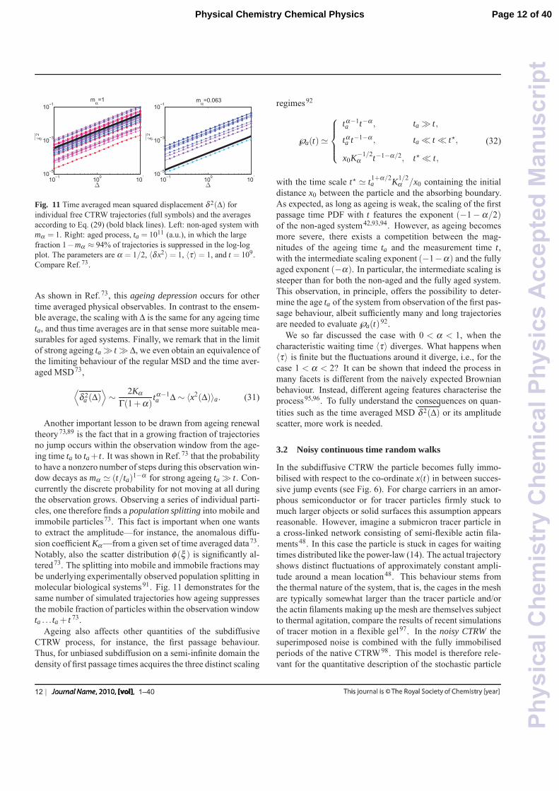
Fig. 11 Time averaged mean squared displacement δ 2(Δ) forindividual free CTRW trajectories (full symbols) and the averagesaccording to Eq. (29) (bold black lines). Left: non-aged system withmα = 1. Right: aged process, ta = 1011 (a.u.), in which the largefraction 1−mα ≈ 94% of trajectories is suppressed in the log-logplot. The parameters are α = 1/2, 〈δx2〉= 1, 〈τ〉= 1, and t = 109.Compare Ref. 73.

As shown in Ref.73, this ageing depression occurs for othertime averaged physical observables. In contrast to the ensem-ble average, the scaling with Δ is the same for any ageing timeta, and thus time averages are in that sense more suitable mea-surables for aged systems. Finally, we remark that in the limitof strong ageing ta � t � Δ, we even obtain an equivalence ofthe limiting behaviour of the regular MSD and the time aver-aged MSD73,⟨

δ 2a (Δ)

⟩∼ 2Kα

Γ(1+α)tα−1a Δ ∼ 〈x2(Δ)〉a. (31)

Another important lesson to be drawn from ageing renewaltheory73,89 is the fact that in a growing fraction of trajectoriesno jump occurs within the observation window from the age-ing time ta to ta+ t. It was shown in Ref.73 that the probabilityto have a nonzero number of steps during this observation win-dow decays as mα � (t/ta)1−α for strong ageing ta � t. Con-currently the discrete probability for not moving at all duringthe observation grows. Observing a series of individual parti-cles, one therefore finds a population splitting into mobile andimmobile particles73. This fact is important when one wantsto extract the amplitude—for instance, the anomalous diffu-sion coefficient Kα —from a given set of time averaged data73.Notably, also the scatter distribution φ(ξ ) is significantly al-tered73. The splitting into mobile and immobile fractions maybe underlying experimentally observed population splitting inmolecular biological systems91. Fig. 11 demonstrates for thesame number of simulated trajectories how ageing suppressesthe mobile fraction of particles within the observation windowta . . . ta + t 73.

Ageing also affects other quantities of the subdiffusiveCTRW process, for instance, the first passage behaviour.Thus, for unbiased subdiffusion on a semi-infinite domain thedensity of first passage times acquires the three distinct scaling

regimes92

℘a(t)�

⎧⎪⎪⎨⎪⎪⎩tα−1a t−α , ta � t,

tαa t−1−α , ta � t � t�,

x0K−1/2α t−1−α/2, t� � t,

(32)

with the time scale t� � t1+α/2a K1/2

α /x0 containing the initialdistance x0 between the particle and the absorbing boundary.As expected, as long as ageing is weak, the scaling of the firstpassage time PDF with t features the exponent (−1−α/2)of the non-aged system42,93,94. However, as ageing becomesmore severe, there exists a competition between the mag-nitudes of the ageing time ta and the measurement time t,with the intermediate scaling exponent (−1−α) and the fullyaged exponent (−α). In particular, the intermediate scaling issteeper than for both the non-aged and the fully aged system.This observation, in principle, offers the possibility to deter-mine the age ta of the system from observation of the first pas-sage behaviour, albeit sufficiently many and long trajectoriesare needed to evaluate ℘a(t)92.

We so far discussed the case with 0 < α < 1, when thecharacteristic waiting time 〈τ〉 diverges. What happens when〈τ〉 is finite but the fluctuations around it diverge, i.e., for thecase 1 < α < 2? It can be shown that indeed the process inmany facets is different from the naively expected Brownianbehaviour. Instead, different ageing features characterise theprocess95,96. To fully understand the consequences on quan-tities such as the time averaged MSD δ 2(Δ) or its amplitudescatter, more work is needed.

3.2 Noisy continuous time random walks

In the subdiffusive CTRW the particle becomes fully immo-bilised with respect to the co-ordinate x(t) in between succes-sive jump events (see Fig. 6). For charge carriers in an amor-phous semiconductor or for tracer particles firmly stuck tomuch larger objects or solid surfaces this assumption appearsreasonable. However, imagine a submicron tracer particle ina cross-linked network consisting of semi-flexible actin fila-ments48. In this case the particle is stuck in cages for waitingtimes distributed like the power-law (14). The actual trajectoryshows distinct fluctuations of approximately constant ampli-tude around a mean location48. This behaviour stems fromthe thermal nature of the system, that is, the cages in the meshare typically somewhat larger than the tracer particle and/orthe actin filaments making up the mesh are themselves subjectto thermal agitation, compare the results of recent simulationsof tracer motion in a flexible gel97. In the noisy CTRW thesuperimposed noise is combined with the fully immobilisedperiods of the native CTRW98. This model is therefore rele-vant for the quantitative description of the stochastic particle

12 | 1–40

Page 12 of 40Physical Chemistry Chemical Physics

Phy

sica

lChe

mis

try

Che

mic

alP

hysi

csA

ccep

ted

Man

uscr

ipt

-6

-4

-2

0

2

0 20 40 60 80 100

x(t)

t / 1000

η=0.001

-6

-4

-2

0

2

0 20 40 60 80 100

x(t)

t / 1000

η=0.005

-6

-4

-2

0

2

0 20 40 60 80 100

x(t)

t / 1000

η=0.01

-6

-4

-2

0

2

0 20 40 60 80 100

x(t)

t / 1000

η=0.1

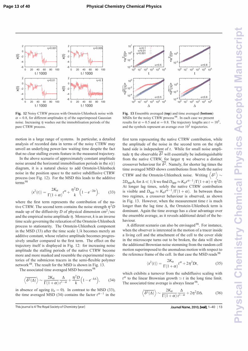
Fig. 12 Noisy CTRW process with Ornstein-Uhlenbeck noise withα = 0.8, for different amplitudes η of the superimposed Gaussiannoise. Increasing η washes out the immobilisation periods of thepure CTRW process.

motion in a large range of systems. In particular, a detailedanalysis of recorded data in terms of the noisy CTRW mayunveil an underlying power-law waiting time despite the factthat no clear stalling events feature in the measured trajectory.

In the above scenario of approximately constant amplitudenoise around the horizontal immobilisation periods in the x(t)diagram, it is a natural choice to add Ornstein-Uhlenbecknoise in the position space to the native subdiffusive CTRWprocess (see Fig. 12). For the MSD this leads to the additiveterms98

〈x2(t)〉= 2Kα

Γ(1+α)tα +

η2Dk

(1− e−2kt

), (33)

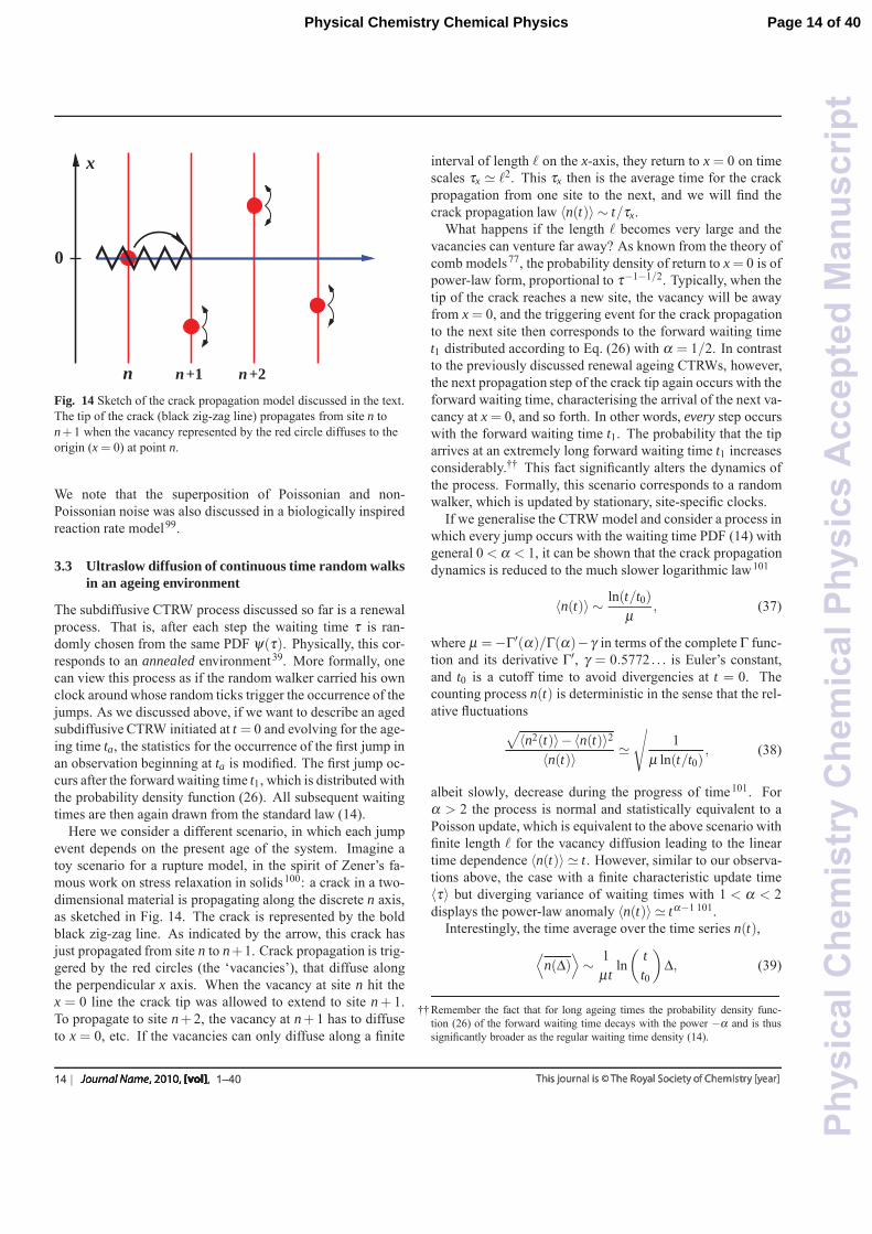
where the first term represents the contribution of the na-tive CTRW. The second term contains the noise strength η2Dmade up of the diffusivity D of physical dimension cm2/secand the empirical noise amplitude η . Moreover, k is an inversetime scale governing the relaxation of the Ornstein-Uhlenbeckprocess to stationarity. The Ornstein-Uhlenbeck componentin the MSD (33) after the time scale 1/k becomes merely anadditive constant, whose relative amplitude becomes progres-sively smaller compared to the first term. The effect on thetrajectory itself is displayed in Fig. 12: for increasing noiseamplitude the stalling periods of the native CTRW becomemore and more masked and resemble the experimental trajec-tories of the submicron tracers in the semi-flexible polymernetwork48. The result for the MSD is shown in Fig. 13.

The associated time averaged MSD becomes98⟨δ 2(Δ)

⟩∼ 2Kα

Γ(1+α)

Δt1−α +

η2Dk

(1− e−kΔ

), (34)

in absence of ageing (ta = 0). In contrast to the MSD (33),the time averaged MSD (34) contains the factor tα−1 in the

10-2

10-1

100

101

100 101 102 103 104 105

<x2 (t)

>

t

α=0.5

η=0.1η=0.01

η=0.001

10-2

100

100 101 102 103 104 105

<x2 (t)

>

t

α=0.8

10-4

10-2

100

100 101 102 103 104 105

< ___

_δ2 (

Δ)>

Δ

α=0.510-4

10-2

100

100 101 102 103 104 105

< ___

_δ2 (

Δ)>

Δ

α=0.8

Fig. 13 Ensemble averaged (top) and time averaged (bottom)MSDs for the noisy CTRW process98. In each case we presentresults for α = 0.5 and α = 0.8. The trajectory lengths are t = 105,and the symbols represent an average over 103 trajectories.

first term representing the native CTRW contribution, whilethe amplitude of the noise in the second term on the righthand side is independent of t. While for small noise ampli-tude η the observable δ 2 will essentially be indistinguishablefrom the native CTRW, for larger η we observe a distinctcrossover behaviour for δ 2. Namely, for shorter lag times thetime averaged MSD shows contributions from both the nativeCTRW and the Ornstein-Uhlenbeck noise. Writing

⟨δ 2

⟩∼

2DappΔ, for Δ� 1/k we find Dapp ≈Kα tα−1/Γ(1+α)+η2D.At longer lag times, solely the native CTRW contributionis visible and Dapp ≈ Kα tα−1/Γ(1 + α). In between thesetwo regimes, a crossover behaviour is observed, as shownin Fig. 13. However, when the measurement time t is muchlonger than the lag time Δ, the Ornstein-Uhlenbeck term isdominant. Again the time average has a clear advantage overthe ensemble average, as it reveals additional detail of the be-haviour.

A different scenario can also be envisaged98. For instance,when the observer is interested in the motion of a tracer insidea living cell and the attachment of the cell to the cover slidein the microscope turns out to be broken, the data will showthe additional Brownian noise stemming from the random cellmotion superimposed to the anomalous motion with respect tothe reference frame of the cell. In that case the MSD reads98

〈x2(t)〉= 2KαΓ(1+α)

tα + 2η2Dt, (35)

which exhibits a turnover from the subdiffusive scaling withtα to the linear Brownian growth � t in the long time limit.The associated time average is always linear98,⟨

δ 2(Δ)⟩∼ 2Kα

Γ(1+α)

Δt1−α + 2η2DΔ. (36)

1–40 | 13

Page 13 of 40 Physical Chemistry Chemical Physics

Phy

sica

lChe

mis

try

Che

mic

alP

hysi

csA

ccep

ted

Man

uscr

ipt

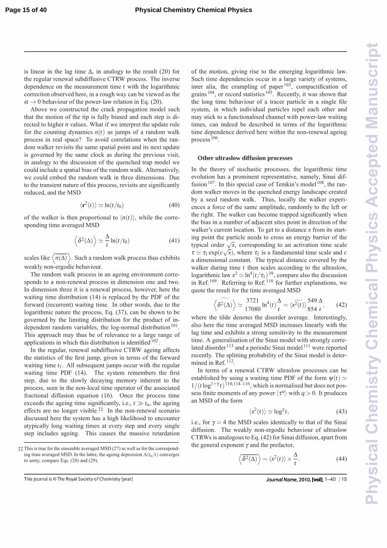
n+1n n+2

x

0

Fig. 14 Sketch of the crack propagation model discussed in the text.The tip of the crack (black zig-zag line) propagates from site n ton+1 when the vacancy represented by the red circle diffuses to theorigin (x = 0) at point n.

We note that the superposition of Poissonian and non-Poissonian noise was also discussed in a biologically inspiredreaction rate model99.

3.3 Ultraslow diffusion of continuous time random walksin an ageing environment

The subdiffusive CTRW process discussed so far is a renewalprocess. That is, after each step the waiting time τ is ran-domly chosen from the same PDF ψ(τ). Physically, this cor-responds to an annealed environment39. More formally, onecan view this process as if the random walker carried his ownclock around whose random ticks trigger the occurrence of thejumps. As we discussed above, if we want to describe an agedsubdiffusive CTRW initiated at t = 0 and evolving for the age-ing time ta, the statistics for the occurrence of the first jump inan observation beginning at ta is modified. The first jump oc-curs after the forward waiting time t1, which is distributed withthe probability density function (26). All subsequent waitingtimes are then again drawn from the standard law (14).

Here we consider a different scenario, in which each jumpevent depends on the present age of the system. Imagine atoy scenario for a rupture model, in the spirit of Zener’s fa-mous work on stress relaxation in solids100: a crack in a two-dimensional material is propagating along the discrete n axis,as sketched in Fig. 14. The crack is represented by the boldblack zig-zag line. As indicated by the arrow, this crack hasjust propagated from site n to n+1. Crack propagation is trig-gered by the red circles (the ‘vacancies’), that diffuse alongthe perpendicular x axis. When the vacancy at site n hit thex = 0 line the crack tip was allowed to extend to site n+ 1.To propagate to site n+ 2, the vacancy at n+ 1 has to diffuseto x = 0, etc. If the vacancies can only diffuse along a finite

interval of length � on the x-axis, they return to x = 0 on timescales τx � �2. This τx then is the average time for the crackpropagation from one site to the next, and we will find thecrack propagation law 〈n(t)〉 ∼ t/τx.

What happens if the length � becomes very large and thevacancies can venture far away? As known from the theory ofcomb models77, the probability density of return to x = 0 is ofpower-law form, proportional to τ−1−1/2. Typically, when thetip of the crack reaches a new site, the vacancy will be awayfrom x = 0, and the triggering event for the crack propagationto the next site then corresponds to the forward waiting timet1 distributed according to Eq. (26) with α = 1/2. In contrastto the previously discussed renewal ageing CTRWs, however,the next propagation step of the crack tip again occurs with theforward waiting time, characterising the arrival of the next va-cancy at x = 0, and so forth. In other words, every step occurswith the forward waiting time t1. The probability that the tiparrives at an extremely long forward waiting time t1 increasesconsiderably.†† This fact significantly alters the dynamics ofthe process. Formally, this scenario corresponds to a randomwalker, which is updated by stationary, site-specific clocks.

If we generalise the CTRW model and consider a process inwhich every jump occurs with the waiting time PDF (14) withgeneral 0 < α < 1, it can be shown that the crack propagationdynamics is reduced to the much slower logarithmic law101

〈n(t)〉 ∼ ln(t/t0)μ

, (37)

where μ =−Γ′(α)/Γ(α)−γ in terms of the complete Γ func-tion and its derivative Γ′, γ = 0.5772 . . . is Euler’s constant,and t0 is a cutoff time to avoid divergencies at t = 0. Thecounting process n(t) is deterministic in the sense that the rel-ative fluctuations√

〈n2(t)〉− 〈n(t)〉2

〈n(t)〉 �√

1μ ln(t/t0)

, (38)

albeit slowly, decrease during the progress of time101. Forα > 2 the process is normal and statistically equivalent to aPoisson update, which is equivalent to the above scenario withfinite length � for the vacancy diffusion leading to the lineartime dependence 〈n(t)〉 � t. However, similar to our observa-tions above, the case with a finite characteristic update time〈τ〉 but diverging variance of waiting times with 1 < α < 2displays the power-law anomaly 〈n(t)〉 � tα−1 101.

Interestingly, the time average over the time series n(t),⟨n(Δ)

⟩∼ 1

μtln(

tt0

)Δ, (39)

†† Remember the fact that for long ageing times the probability density func-tion (26) of the forward waiting time decays with the power −α and is thussignificantly broader as the regular waiting time density (14).

14 | 1–40

Page 14 of 40Physical Chemistry Chemical Physics

Phy

sica

lChe

mis

try

Che

mic

alP

hysi

csA

ccep

ted

Man

uscr

ipt

is linear in the lag time Δ, in analogy to the result (20) forthe regular renewal subdiffusive CTRW process. The inversedependence on the measurement time t with the logarithmiccorrection observed here, in a rough way can be viewed as theα → 0 behaviour of the power-law relation in Eq. (20).

Above we constructed the crack propagation model suchthat the motion of the tip is fully biased and each step is di-rected to higher n values. What if we interpret the update rulefor the counting dynamics n(t) as jumps of a random walkprocess in real space? To avoid correlations when the ran-dom walker revisits the same spatial point and its next updateis governed by the same clock as during the previous visit,in analogy to the discussion of the quenched trap model wecould include a spatial bias of the random walk. Alternatively,we could embed the random walk in three dimensions. Dueto the transient nature of this process, revisits are significantlyreduced, and the MSD

〈r2(t)〉 � ln(t/t0) (40)

of the walker is then proportional to 〈n(t)〉, while the corre-sponding time averaged MSD⟨

δ 2(Δ)⟩� Δ

tln(t/t0) (41)

scales like⟨

n(Δ)⟩

. Such a random walk process thus exhibitsweakly non-ergodic behaviour.

The random walk process in an ageing environment corre-sponds to a non-renewal process in dimension one and two.In dimension three it is a renewal process, however, here thewaiting time distribution (14) is replaced by the PDF of theforward (recurrent) waiting time. In other words, due to thelogarithmic nature the process, Eq. (37), can be shown to begoverned by the limiting distribution for the product of in-dependent random variables, the log-normal distribution101.This approach may thus be of relevance to a large range ofapplications in which this distribution is identified102.

In the regular, renewal subdiffusive CTRW ageing affectsthe statistics of the first jump, given in terms of the forwardwaiting time t1. All subsequent jumps occur with the regularwaiting time PDF (14). The system remembers the firststep, due to the slowly decaying memory inherent to theprocess, seen in the non-local time operator of the associatedfractional diffusion equation (16). Once the process timeexceeds the ageing time significantly, i.e., t � ta, the ageingeffects are no longer visible.‡‡ In the non-renewal scenariodiscussed here the system has a high likelihood to encounteratypically long waiting times at every step and every singlestep includes ageing. This causes the massive retardation

‡‡ This is true for the ensemble averaged MSD (27) as well as for the correspond-ing time averaged MSD. In the latter, the ageing depression Λ(ta/t) convergesto unity, compare Eqs. (28) and (29).

of the motion, giving rise to the emerging logarithmic law.Such time dependencies occur in a large variety of systems,inter alia, the crumpling of paper103, compactification ofgrains104, or record statistics105. Recently, it was shown thatthe long time behaviour of a tracer particle in a single filesystem, in which individual particles repel each other andmay stick to a functionalised channel with power-law waitingtimes, can indeed be described in terms of the logarithmictime dependence derived here within the non-renewal ageingprocess106.

Other ultraslow diffusion processes

In the theory of stochastic processes, the logarithmic timeevolution has a prominent representative, namely, Sinai dif-fusion107. In this special case of Temkin’s model108, the ran-dom walker moves in the quenched energy landscape createdby a seed random walk. Thus, locally the walker experi-ences a force of the same amplitude, randomly to the left orthe right. The walker can become trapped significantly whenthe bias in a number of adjacent sites point in direction of thewalker’s current location. To get to a distance x from its start-ing point the particle needs to cross an energy barrier of thetypical order

√x, corresponding to an activation time scale

τ � τ1 exp(c√

x), where τ1 is a fundamental time scale and ca dimensional constant. The typical distance covered by thewalker during time t then scales according to the ultraslow,logarithmic law x2 � ln4(t/τ1)

39, compare also the discussionin Ref.109. Referring to Ref.110 for further explanations, wequote the result for the time averaged MSD˜⟨

δ 2(Δ)⟩� 3721

17080ln4(t)

Δt= ˜〈x2(t)〉549

854Δt, (42)

where the tilde denotes the disorder average. Interestingly,also here the time averaged MSD increases linearly with thelag time and exhibits a strong sensitivity to the measurementtime. A generalisation of the Sinai model with strongly corre-lated disorder113 and a periodic Sinai model111 were reportedrecently. The splitting probability of the Sinai model is deter-mined in Ref.112.

In terms of a renewal CTRW ultraslow processes can beestablished by using a waiting time PDF of the form ψ(t) �1/(t log1+γ t)110,114–116, which is normalised but does not pos-sess finite moments of any power 〈τq〉 with q > 0. It producesan MSD of the form

〈x2(t)〉 � logγ t, (43)

i.e., for γ = 4 the MSD scales identically to that of the Sinaidiffusion. The weakly non-ergodic behaviour of ultraslowCTRWs is analogous to Eq. (42) for Sinai diffusion, apart fromthe general exponent γ and the prefactor,⟨

δ 2(Δ)⟩∼ 〈x2(t)〉× Δ

t. (44)

1–40 | 15

Page 15 of 40 Physical Chemistry Chemical Physics

Phy

sica

lChe

mis

try

Che

mic

alP

hysi

csA

ccep

ted

Man

uscr

ipt

The time averaged MSD, the localisation of the diffusion par-ticle, as well as the ergodic properties of both Sinai and ul-traslow CTRW diffusion are analysed in Ref.110, discussingsome of the fundamental differences between time averagesrecorded in annealed versus quenched environments.

Finally, ultraslow diffusion can also be effected by iterativedynamics maps, as shown by Drager and Klafter116. Insteadof the power-law maps with a single exponent z discussedin Ref.79, however, ultraslow diffusion emerges when an en-tire hierarchy of exponents is considered. In very dense two-dimensional lattice gas systems, ultraslow diffusion emerges,as well117.

3.4 Correlated continuous time random walks

Another way to break the renewal character of the standardCTRW process is to introduce correlations between successivewaiting times. Correlations appear naturally in the motion be-haviour of higher animals or humans, or in the dynamics offinancial markets. They are also present for particles diffus-ing in quenched disorder, compare the above discussion of thequenched trap model or Sinai diffusion. It is therefore conse-quent to consider non-renewal CTRW processes with built-incorrelations. This can be achieved by extension of the sub-ordination of the physical time to the number of steps of theprocess118,119. An alternative approach is the following.

Assume that successive waiting times are correlated in away that waiting time τi is given by waiting time τi−1 mod-ified by a small increment, δτi, that is, τi = τi−1 + δτi. Theincrements δτi may be positive or negative. Successive wait-ing times are thus correlated: a short waiting time is followedby a similarly short one, and vice versa for a long waitingtime. This approach corresponds in fact to a random walk inthe space of waiting times, and we can write the current wait-ing τi time as the sum of increments120–122

τi =∣∣∣δτ1 + δτ2 + . . .+ δτi−1

∣∣∣. (45)

The absolute value occurs here as waiting times always have tobe positive. These increments δτi are then chosen to follow agiven probability distribution. We may, for instance, considerthe symmetric Levy stable law defined in terms of its Fouriertransform as exp

(−cγ |k|γ). The process can then be shown

to produce a power-law MSD of the form (8) with anomalousdiffusion exponent

α =γ

1+ γ, (46)

whose range spans from zero (for γ = 0) to 2/3 (for γ = 2)and thus leaves a gap to normal diffusion120,121. Brownianmotion with α = 1 in this model can only be restored by com-pletely breaking the correlations120. In the limit γ = 2 themode relaxation is of stretched exponential form, P(k, t) �

-12-8-4 0 4 8

0 500 1000

x(t)

t

-20

-10

0

10

20

0 500 1000

x(t)

t

0 50

100 150 200 250

0 20 40 60 80 100 120

τ i

i

0 2 4 6 8

10

0 50 100 150 200 250

τ i

i

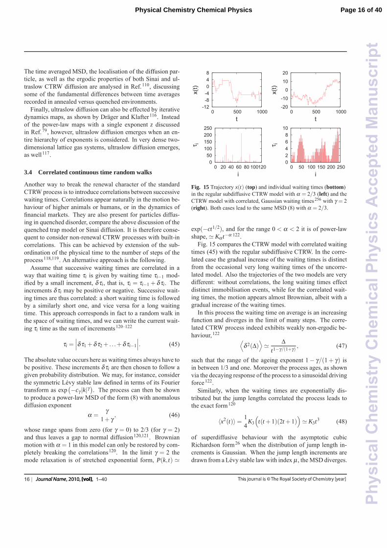
Fig. 15 Trajectory x(t) (top) and individual waiting times (bottom)in the regular subdiffusive CTRW model with α = 2/3 (left) and theCTRW model with correlated, Gaussian waiting times256 with γ = 2(right). Both cases lead to the same MSD (8) with α = 2/3.

exp(−ct1/2), and for the range 0 < α < 2 it is of power-lawshape, � Kα t−α 122.

Fig. 15 compares the CTRW model with correlated waitingtimes (45) with the regular subdiffusive CTRW. In the corre-lated case the gradual increase of the waiting times is distinctfrom the occasional very long waiting times of the uncorre-lated model. Also the trajectories of the two models are verydifferent: without correlations, the long waiting times effectdistinct immobilisation events, while for the correlated wait-ing times, the motion appears almost Brownian, albeit with agradual increase of the waiting times.

In this process the waiting time on average is an increasingfunction and diverges in the limit of many steps. The corre-lated CTRW process indeed exhibits weakly non-ergodic be-haviour,122 ⟨

δ 2(Δ)⟩� Δ

t1−γ/(1+γ) , (47)

such that the range of the ageing exponent 1− γ/(1+ γ) isin between 1/3 and one. Moreover the process ages, as shownvia the decaying response of the process to a sinusoidal drivingforce122.

Similarly, when the waiting times are exponentially dis-tributed but the jump lengths correlated the process leads tothe exact form120

〈x2(t)〉= 14

K3

(t(t + 1)(2t+ 1)

)� K3t3 (48)

of superdiffusive behaviour with the asymptotic cubicRichardson form26 when the distribution of jump length in-crements is Gaussian. When the jump length increments aredrawn from a Levy stable law with index μ , the MSD diverges.

16 | 1–40

Page 16 of 40Physical Chemistry Chemical Physics

Phy

sica

lChe

mis

try

Che

mic

alP

hysi

csA

ccep

ted

Man

uscr

ipt

From fractional oder moments one can derive the scaling rela-tion x2 ∼ t(1+μ)/μ . For the case μ = 2 the weakly non-ergodicform of the MSD⟨

δ 2(Δ)⟩=

3K3

4Δ2t+K3

(Δ4+

3Δ2

4− Δ3

4

)∼ 3K3

4Δ2t (49)

was obtained exactly, and the expansion is valid for Δ � t 120.

3.5 Superdiffusive continuous time random walks andultraweak ergodicity breaking

For completeness we also consider superdiffusive renewalCTRW processes. To that end we note that the introduction ofa waiting time distribution into a standard random walk pro-cess at most leads to a subdiffusive behaviour when the firstmoment of the waiting time PDF ψ(τ) diverges. Superdiffu-sion cannot be achieved within the approach of a generalisedwaiting time concept. There exist, however, two pathways toextend the CTRW model to superdiffusion.

The first way is to modify the distribution of jump lengths.All CTRW processes considered so far (apart from the caseof correlated jump lengths in the preceding section) corre-spond to the motion on a lattice, or in continuous space witha jump length PDF that possesses a finite variance 〈δx2〉 andzero mean 〈δx〉. What if we choose a jump length distribu-tion λ (x), for which the variance 〈δx2〉 diverges? Consider aLevy stable form with the asymptotic power-law behaviourλ (x) � 1/|x|1+μ of the jump lengths with the stable index0 < μ ≤ 2. When the waiting time PDF has finite moments,this process was called a Levy flight by Mandelbrot124. Thedivergence of the jump length variance translates into the di-vergence of the second moment of the PDF P(x, t)125, andonly fractional order moments 〈|x|κ〉 with 0 < κ < μ exist42.The trajectory of a Levy flight is fractal (see below) of Haus-dorff dimension μ . A single trajectory therefore never fullycovers an embedding space whose dimension is larger thanμ . This is particularly relevant in the two-dimensional world,in which effectively most human and animal motion occurs.There exist also several works considering the combination ofa diverging characteristic waiting time 〈τ〉 with a Levy stabledistribution of jump lengths, either in terms of fractional dif-fusion equations126 or via using subordination arguments127.Due to its fractality a single Levy flight trajectory cannot visitall points in space when the stable index μ is smaller thanthe embedding dimension d. Under confinement to a finitearea, Levy flights are ergodic128, and the convergence to theergodic state can be analysed in terms of the apparent fractaldimension or in terms of the first passage dynamics129. Thedivergence of 〈δx2〉 as well as the ensuing non-ergodicity ofLevy flights can be rectified by a cutoff in the jump lengthPDF130 or by dissipative non-linearities131. Such stochastic

processes behave like a Levy flight until the regularisation ofthe jump length PDF comes into effect.

The alternative approach is to introduce a coupling betweenjump lengths and waiting times. In subdiffusive CTRWs de-scribed previously the waiting time and jump length PDFs en-ter in the multiplicative form ψ(δx,τ) = ψ(τ)λ (δx)43. In-troducing a functional dependence between waiting times τand jump lengths δx, this spatiotemporal coupling preservesthe renewal property of CTRW processes but due to penalis-ing long jumps—associating them with long waiting times—yields a finite MSD43,132. The simplest choice is the couplingψ(δx,τ) = 1

2 ψ(τ)δ (|δx|− vτ), in which the velocity v is in-troduced. It bestows a propagating horizon to the process inthe form of two travelling δ peaks with decaying amplitude.For waiting time PDFs ψ(τ)� τ−1−α with 1 < α < 2, in be-tween these peaks, a Levy stable distribution is building up133.Also Levy walks are non-ergodic, albeit in a way, that is dif-ferent from the above discussed non-ergodic behaviour. To seethis, we first recall that for a waiting time PDF of the power-law form ψ(τ) = τ−1−α their MSD scales134,135

〈x2(t)〉 �{

v2(1−α)t2, 0 < α < 12K3−αt3−α , 1 < α < 2 . (50)

The associated time averaged MSD in the ballistic phase with0 < α < 1 scales like ⟨

δ 2(Δ)⟩∼ v2Δ2, (51)

with a higher order correction scaling with Δ2(Δ/t)2−α 136,137.In the enhanced diffusion phase 1 < α < 2 the result is136–138⟨

δ 2(Δ)⟩∼ 2K3−α

α − 1Δ3−α . (52)

In both the ballistic and enhanced diffusive phases the MSDdiffers from the time averaged MSD merely by a factor of1/|α − 1|. This phenomenon may be referred to as ultra-weak ergodicity breaking138. Note that an analogous resultwas obtained by Zumofen and Klafter for Levy walks withstationary and non-stationary initial conditions139, comparethe discussion in Ref.138. To leading order, the time averagedMSDs (51) and (52) do not exhibit ageing in the sense thatthe measurement time t does not appear explicitly, in contrastto the corresponding forms for the subdiffusive CTRW pro-cesses discussed above. Further physical properties of Levywalks, in particular, the amplitude scatter of the time averagedMSD, are studied in Refs.138,140. Additional recent studies ofLevy walks analyse their response to an external bias and thepower spectral properties136–138,140.

Levy flights and walks are used as statistical models inmany fields, for example, to quantify blind search processesof animals for sparse food141–143. In the science of movementecology, the so-called Levy foraging hypothesis has become

1–40 | 17

Page 17 of 40 Physical Chemistry Chemical Physics

Phy

sica

lChe

mis

try

Che

mic

alP

hysi

csA

ccep

ted

Man

uscr

ipt

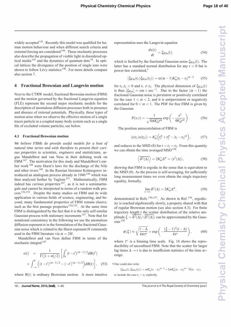
widely accepted141. Recently this model was qualified for hu-man motion behaviour and when different search criteria andexternal forcing are considered144. These stochastic processesalso describe the propagation of visible light in disordered op-tical media145 and the dynamics of quantum dots34. In opti-cal lattices the divergence of the position of single ions wereshown to follow Levy statistics146. For more details comparealso section 7.

4 Fractional Brownian and Langevin motion

Next to the CTRW model, fractional Brownian motion (FBM)and the motion governed by the fractional Langevin equation(FLE) represent the second major stochastic models for thedescription of anomalous diffusion processes both in presenceand absence of external potentials. Physically, these types ofmotion arise when we observe the effective motion of a singletracer particle in a coupled many-body system such as a singlefile of excluded volume particles, see below.

4.1 Fractional Brownian motion

We believe FBMs do provide useful models for a host ofnatural time series and wish therefore to present their curi-ous properties to scientists, engineers and statisticians, ar-gue Mandelbrot and van Ness in their defining work onFBM147. The motivation for this study and Mandelbrot’s ear-lier work148 were Hurst’s laws for the discharge of the Nileand other rivers149. In the Russian literature Kolmogorov in-troduced an analogous process already in 1940150 which wasthen analysed further by Yaglom151. Mathematically, FBMindeed has curious properties147, as it is not a semimartin-gale and cannot be interpreted in terms of a random walk pro-cess152,153. Despite the many studies on FBM and its wideapplication in various fields of science, engineering, and be-yond, many fundamental properties of FBM remain elusive,such as the first passage properties154,155. At the same timeFBM is distinguished by the fact that it is the only self-similarGaussian process with stationary increments147. Note that fornotational consistency in the following we use the anomalousdiffusion exponent α in the formulation of the fractional Gaus-sian noise which is related to the Hurst exponent H commonlyused in the FBM literature via α = 2H.

Mandelbrot and van Ness define FBM in terms of thestochastic integral147

x(t) =1

Γ([1+α]/2)

[∫ t

0(t − t ′)(α−1)/2dB(t ′)

+

∫ 0

−∞

((t − t ′)(α−1)/2 − (−t ′)(α−1)/2

)dB(t)

], (53)

where B(t) is ordinary Brownian motion. A more intuitive

representation uses the Langevin equation

dx(t)dt

= ξfGn(t), (54)

which is fuelled by the fractional Gaussian noise ξfGn(t). Thelatter has a standard normal distribution for any t > 0 but ispower-law correlated,†

〈ξfGn(t1)ξfGn(t2)〉= α(α − 1)K∗α |t1 − t2|α−2 (55)

for t1, t2 > 0 and t1 �= t2. The physical dimension of ξfGn(t)is thus [ξfGn] = cm× sec−1. Due to the factor (α − 1) thefractional Gaussian noise is persistent or positively correlatedfor the case 1 < α < 2, and it is antipersistent or negativelycorrelated for 0 < α < 1. The PDF for free FBM is given bythe Gaussian

P(x, t) =1√

4πK∗αtα exp

(− x2

4K∗αtα

). (56)

The position autocorrelation of FBM is

〈x(t1)x(t2)〉= K∗α

(tα1 + tα

2 −|t1 − t2|α), (57)

and reduces to the MSD (8) for t = t1 = t2. From this quantitywe can obtain the time averaged MSD156⟨

δ 2(Δ)⟩= 2K∗

α Δα = 〈x2(Δ)〉, (58)

showing that FBM is ergodic in the sense that is equivalent tothe MSD (8). As the process is self-averaging, for sufficientlylong measurement times we even obtain the single trajectoryequality, formally,

limt→∞

δ 2(Δ) = 2K∗α Δα . (59)

demonstrated in Refs.156,157. As shown in Ref.156, ergodic-ity is reached algebraically slowly, a property shared with thatof regular Brownian motion (see also section 4.3). For finitetrajectory length t the scatter distribution of the relative am-plitude ξ = δ 2(Δ)/〈δ 2(Δ)〉 can be approximated by the Gaus-sian158

φ(ξ )≈√

t −Δ4πτ∗

× exp(− (ξ − 1)2(t −Δ)

4τ∗

), (60)

where τ∗ is a binning time scale. Fig. 16 shows the repro-ducibility of unconfined FBM. Note that the scatter for largerlag times Δ → t is due to insufficient statistics of the time av-erage.

† One could also write

〈ξfGn(t1)ξfGn(t2)〉= αK∗α |t1 − t2|α−2 +2αK∗

α |t1 − t2|α−1δ (t1 − t2),

to include the case t1 = t2 explicitly.

18 | 1–40

Page 18 of 40Physical Chemistry Chemical Physics

Phy

sica

lChe

mis

try

Che

mic

alP

hysi

csA

ccep

ted

Man

uscr

ipt

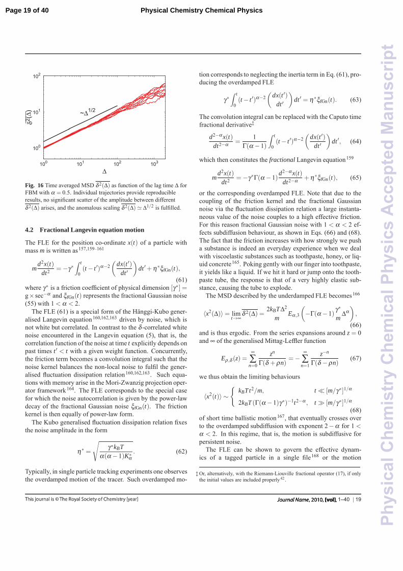
100

101

102

100 101 102 103

___

_δ2 (

Δ)

Δ

~Δ1/2

Fig. 16 Time averaged MSD δ 2(Δ) as function of the lag time Δ forFBM with α = 0.5. Individual trajectories provide reproducibleresults, no significant scatter of the amplitude between differentδ 2(Δ) arises, and the anomalous scaling δ 2(Δ)� Δ1/2 is fulfilled.

4.2 Fractional Langevin equation motion

The FLE for the position co-ordinate x(t) of a particle withmass m is written as157,159–161

md2x(t)

dt2 =−γ∗∫ t

0(t − t ′)α−2

(dx(t ′)

dt ′

)dt ′+η∗ξfGn(t),

(61)where γ∗ is a friction coefficient of physical dimension [γ∗] =g× sec−α and ξfGn(t) represents the fractional Gaussian noise(55) with 1 < α < 2.

The FLE (61) is a special form of the Hanggi-Kubo gener-alised Langevin equation160,162,163 driven by noise, which isnot white but correlated. In contrast to the δ -correlated whitenoise encountered in the Langevin equation (5), that is, thecorrelation function of the noise at time t explicitly depends onpast times t ′ < t with a given weight function. Concurrently,the friction term becomes a convolution integral such that thenoise kernel balances the non-local noise to fulfil the gener-alised fluctuation dissipation relation160,162,163. Such equa-tions with memory arise in the Mori-Zwanzig projection oper-ator framework164. The FLE corresponds to the special casefor which the noise autocorrelation is given by the power-lawdecay of the fractional Gaussian noise ξfGn(t). The frictionkernel is then equally of power-law form.

The Kubo generalised fluctuation dissipation relation fixesthe noise amplitude in the form

η∗ =

√γ∗kBT

α(α − 1)K∗α. (62)

Typically, in single particle tracking experiments one observesthe overdamped motion of the tracer. Such overdamped mo-

tion corresponds to neglecting the inertia term in Eq. (61), pro-ducing the overdamped FLE

γ∗∫ t

0(t − t ′)α−2

(dx(t ′)

dt ′

)dt ′ = η∗ξfGn(t). (63)

The convolution integral can be replaced with the Caputo timefractional derivative‡

d2−αx(t)dt2−α =

1Γ(α − 1)

∫ t

0(t − t ′)α−2

(dx(t ′)

dt ′

)dt ′, (64)

which then constitutes the fractional Langevin equation159

md2x(t)

dt2 =−γ∗Γ(α − 1)d2−αx(t)

dt2−α +η∗ξfGn(t), (65)

or the corresponding overdamped FLE. Note that due to thecoupling of the friction kernel and the fractional Gaussiannoise via the fluctuation dissipation relation a large instanta-neous value of the noise couples to a high effective friction.For this reason fractional Gaussian noise with 1 < α < 2 ef-fects subdiffusion behaviour, as shown in Eqs. (66) and (68).The fact that the friction increases with how strongly we pusha substance is indeed an everyday experience when we dealwith viscoelastic substances such as toothpaste, honey, or liq-uid concrete165. Poking gently with our finger into toothpaste,it yields like a liquid. If we hit it hard or jump onto the tooth-paste tube, the response is that of a very highly elastic sub-stance, causing the tube to explode.

The MSD described by the underdamped FLE becomes166

〈x2(Δ)〉= limt→∞

δ 2(Δ) =2kBTΔ2

mEα ,3

(−Γ(α − 1)

γ∗

mΔα

),

(66)and is thus ergodic. From the series expansions around z = 0and ∞ of the generalised Mittag-Leffler function

Eρ ,δ (z) =∞

∑n=0

zn

Γ(δ +ρn)=−

∞

∑n=1

z−n

Γ(δ −ρn)(67)

we thus obtain the limiting behaviours

〈x2(t)〉 ∼{

kBTt2/m, t � [m/γ∗]1/α

2kBT (Γ(α − 1)γ∗)−1t2−α , t � [m/γ∗]1/α

(68)of short time ballistic motion167, that eventually crosses overto the overdamped subdiffusion with exponent 2−α for 1 <α < 2. In this regime, that is, the motion is subdiffusive forpersistent noise.

The FLE can be shown to govern the effective dynam-ics of a tagged particle in a single file168 or the motion

‡ Or, alternatively, with the Riemann-Liouville fractional operator (17), if onlythe initial values are included properly 42 .

1–40 | 19

Page 19 of 40 Physical Chemistry Chemical Physics

Phy

sica

lChe

mis

try

Che

mic

alP

hysi

csA

ccep

ted

Man

uscr

ipt

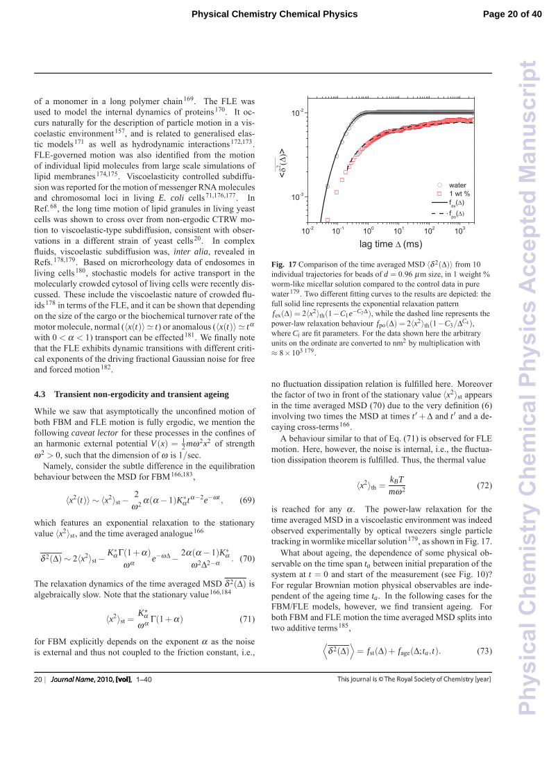
of a monomer in a long polymer chain169. The FLE wasused to model the internal dynamics of proteins170. It oc-curs naturally for the description of particle motion in a vis-coelastic environment157, and is related to generalised elas-tic models171 as well as hydrodynamic interactions172,173.FLE-governed motion was also identified from the motionof individual lipid molecules from large scale simulations oflipid membranes174,175. Viscoelasticity controlled subdiffu-sion was reported for the motion of messenger RNA moleculesand chromosomal loci in living E. coli cells71,176,177. InRef.68, the long time motion of lipid granules in living yeastcells was shown to cross over from non-ergodic CTRW mo-tion to viscoelastic-type subdiffusion, consistent with obser-vations in a different strain of yeast cells20. In complexfluids, viscoelastic subdiffusion was, inter alia, revealed inRefs.178,179. Based on microrheology data of endosomes inliving cells180, stochastic models for active transport in themolecularly crowded cytosol of living cells were recently dis-cussed. These include the viscoelastic nature of crowded flu-ids178 in terms of the FLE, and it can be shown that dependingon the size of the cargo or the biochemical turnover rate of themotor molecule, normal (〈x(t)〉 � t) or anomalous (〈x(t)〉 � tα

with 0 < α < 1) transport can be effected181. We finally notethat the FLE exhibits dynamic transitions with different criti-cal exponents of the driving fractional Gaussian noise for freeand forced motion182.

4.3 Transient non-ergodicity and transient ageing

While we saw that asymptotically the unconfined motion ofboth FBM and FLE motion is fully ergodic, we mention thefollowing caveat lector for these processes in the confines ofan harmonic external potential V (x) = 1

2mω2x2 of strengthω2 > 0, such that the dimension of ω is 1/sec.

Namely, consider the subtle difference in the equilibrationbehaviour between the MSD for FBM166,183,

〈x2(t)〉 ∼ 〈x2〉st − 2ω2 α(α − 1)K∗

αtα−2e−ωt , (69)

which features an exponential relaxation to the stationaryvalue 〈x2〉st, and the time averaged analogue166

δ 2(Δ)∼ 2〈x2〉st − K∗α Γ(1+α)

ωα e−ωΔ − 2α(α − 1)K∗α

ω2Δ2−α . (70)

The relaxation dynamics of the time averaged MSD δ 2(Δ) isalgebraically slow. Note that the stationary value166,184

〈x2〉st =K�

αωα Γ(1+α) (71)

for FBM explicitly depends on the exponent α as the noiseis external and thus not coupled to the friction constant, i.e.,

����

����

���

���

���

���

����

����

�������

��������

��� �

� ��

��

��������� ����

Fig. 17 Comparison of the time averaged MSD 〈δ 2(Δ)〉 from 10individual trajectories for beads of d = 0.96 μm size, in 1 weight %worm-like micellar solution compared to the control data in purewater179. Two different fitting curves to the results are depicted: thefull solid line represents the exponential relaxation patternfex(Δ) = 2〈x2〉th(1−C1e−C2Δ), while the dashed line represents thepower-law relaxation behaviour fpo(Δ) = 2〈x2〉th(1−C3/ΔC4),where Ci are fit parameters. For the data shown here the arbitraryunits on the ordinate are converted to nm2 by multiplication with≈ 8×103 179.

no fluctuation dissipation relation is fulfilled here. Moreoverthe factor of two in front of the stationary value 〈x2〉st appearsin the time averaged MSD (70) due to the very definition (6)involving two times the MSD at times t ′+Δ and t ′ and a de-caying cross-terms166.

A behaviour similar to that of Eq. (71) is observed for FLEmotion. Here, however, the noise is internal, i.e., the fluctua-tion dissipation theorem is fulfilled. Thus, the thermal value

〈x2〉th =kBTmω2 (72)

is reached for any α . The power-law relaxation for thetime averaged MSD in a viscoelastic environment was indeedobserved experimentally by optical tweezers single particletracking in wormlike micellar solution179, as shown in Fig. 17.

What about ageing, the dependence of some physical ob-servable on the time span ta between initial preparation of thesystem at t = 0 and start of the measurement (see Fig. 10)?For regular Brownian motion physical observables are inde-pendent of the ageing time ta. In the following cases for theFBM/FLE models, however, we find transient ageing. Forboth FBM and FLE motion the time averaged MSD splits intotwo additive terms185,⟨

δ 2(Δ)⟩= fst(Δ)+ fage(Δ;ta, t). (73)

20 | 1–40

Page 20 of 40Physical Chemistry Chemical Physics

Phy

sica

lChe

mis

try

Che

mic

alP

hysi

csA

ccep

ted

Man

uscr

ipt

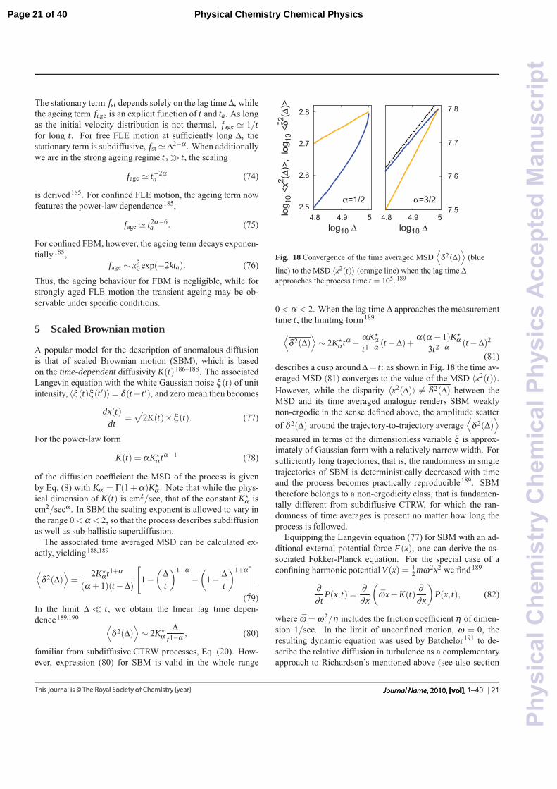
The stationary term fst depends solely on the lag time Δ, whilethe ageing term fage is an explicit function of t and ta. As longas the initial velocity distribution is not thermal, fage � 1/tfor long t. For free FLE motion at sufficiently long Δ, thestationary term is subdiffusive, fst � Δ2−α . When additionallywe are in the strong ageing regime ta � t, the scaling

fage � t−2αa (74)

is derived185. For confined FLE motion, the ageing term nowfeatures the power-law dependence185,

fage � t2α−6a . (75)

For confined FBM, however, the ageing term decays exponen-tially185,

fage ∼ x20 exp(−2kta). (76)

Thus, the ageing behaviour for FBM is negligible, while forstrongly aged FLE motion the transient ageing may be ob-servable under specific conditions.

5 Scaled Brownian motion

A popular model for the description of anomalous diffusionis that of scaled Brownian motion (SBM), which is basedon the time-dependent diffusivity K(t)186–188. The associatedLangevin equation with the white Gaussian noise ξ (t) of unitintensity, 〈ξ (t)ξ (t ′)〉= δ (t− t ′), and zero mean then becomes

dx(t)dt

=√

2K(t)× ξ (t). (77)

For the power-law form

K(t) = αK�α tα−1 (78)

of the diffusion coefficient the MSD of the process is givenby Eq. (8) with Kα = Γ(1+α)K�

α . Note that while the phys-ical dimension of K(t) is cm2/sec, that of the constant K�

α iscm2/secα . In SBM the scaling exponent is allowed to vary inthe range 0<α < 2, so that the process describes subdiffusionas well as sub-ballistic superdiffusion.

The associated time averaged MSD can be calculated ex-actly, yielding188,189

⟨δ 2(Δ)

⟩=

2K�α t1+α

(α + 1)(t−Δ)

[1−

(Δt

)1+α−(

1− Δt

)1+α].

(79)In the limit Δ � t, we obtain the linear lag time depen-dence189,190 ⟨

δ 2(Δ)⟩∼ 2K�

αΔ

t1−α , (80)

familiar from subdiffusive CTRW processes, Eq. (20). How-ever, expression (80) for SBM is valid in the whole range

2.5

2.6

2.7

2.8

4.8 4.9 5log 1

0 <x

2 (Δ)>

, lo

g 10

<δ- 2(Δ

)>

log10 Δ

α=1/2

4.8 4.9 5 7.5

7.6

7.7

7.8

log10 Δ

α=3/2

Fig. 18 Convergence of the time averaged MSD⟨

δ 2(Δ)⟩

(blueline) to the MSD 〈x2(t)〉 (orange line) when the lag time Δapproaches the process time t = 105. 189

0 < α < 2. When the lag time Δ approaches the measurementtime t, the limiting form189⟨

δ 2(Δ)⟩∼ 2K�

α tα − αK�α

t1−α (t −Δ)+α(α − 1)K�

α3t2−α (t −Δ)2

(81)describes a cusp around Δ= t: as shown in Fig. 18 the time av-eraged MSD (81) converges to the value of the MSD 〈x2(t)〉.However, while the disparity 〈x2(Δ)〉 �= δ 2(Δ) between theMSD and its time averaged analogue renders SBM weaklynon-ergodic in the sense defined above, the amplitude scatterof δ 2(Δ) around the trajectory-to-trajectory average

⟨δ 2(Δ)

⟩measured in terms of the dimensionless variable ξ is approx-imately of Gaussian form with a relatively narrow width. Forsufficiently long trajectories, that is, the randomness in singletrajectories of SBM is deterministically decreased with timeand the process becomes practically reproducible189. SBMtherefore belongs to a non-ergodicity class, that is fundamen-tally different from subdiffusive CTRW, for which the ran-domness of time averages is present no matter how long theprocess is followed.

Equipping the Langevin equation (77) for SBM with an ad-ditional external potential force F(x), one can derive the as-sociated Fokker-Planck equation. For the special case of aconfining harmonic potential V (x) = 1

2 mω2x2 we find189

∂∂ t

P(x, t) =∂∂x

(ωx+K(t)

∂∂x

)P(x, t), (82)

where ω = ω2/η includes the friction coefficient η of dimen-sion 1/sec. In the limit of unconfined motion, ω = 0, theresulting dynamic equation was used by Batchelor191 to de-scribe the relative diffusion in turbulence as a complementaryapproach to Richardson’s mentioned above (see also section

1–40 | 21

Page 21 of 40 Physical Chemistry Chemical Physics

Phy

sica

lChe

mis

try

Che

mic

alP

hysi

csA

ccep

ted

Man

uscr

ipt

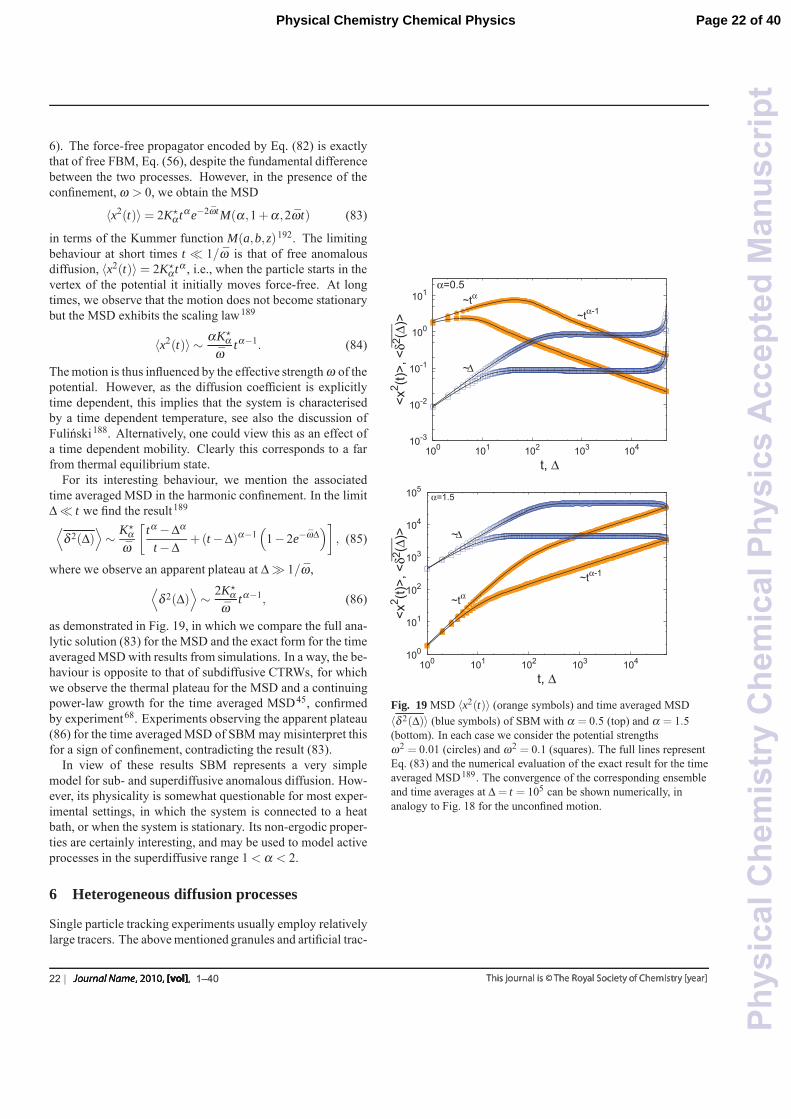
6). The force-free propagator encoded by Eq. (82) is exactlythat of free FBM, Eq. (56), despite the fundamental differencebetween the two processes. However, in the presence of theconfinement, ω > 0, we obtain the MSD

〈x2(t)〉= 2K�α tαe−2ωtM(α,1+α,2ωt) (83)

in terms of the Kummer function M(a,b,z)192. The limitingbehaviour at short times t � 1/ω is that of free anomalousdiffusion, 〈x2(t)〉= 2K�

αtα , i.e., when the particle starts in thevertex of the potential it initially moves force-free. At longtimes, we observe that the motion does not become stationarybut the MSD exhibits the scaling law189

〈x2(t)〉 ∼ αK�α

ωtα−1. (84)

The motion is thus influenced by the effective strength ω of thepotential. However, as the diffusion coefficient is explicitlytime dependent, this implies that the system is characterisedby a time dependent temperature, see also the discussion ofFulinski188. Alternatively, one could view this as an effect ofa time dependent mobility. Clearly this corresponds to a farfrom thermal equilibrium state.

For its interesting behaviour, we mention the associatedtime averaged MSD in the harmonic confinement. In the limitΔ � t we find the result189⟨

δ 2(Δ)⟩∼ K�

αω

[tα −Δα

t −Δ+(t −Δ)α−1

(1− 2e−ωΔ

)], (85)

where we observe an apparent plateau at Δ � 1/ω,⟨δ 2(Δ)

⟩∼ 2K�

αω

tα−1, (86)

as demonstrated in Fig. 19, in which we compare the full ana-lytic solution (83) for the MSD and the exact form for the timeaveraged MSD with results from simulations. In a way, the be-haviour is opposite to that of subdiffusive CTRWs, for whichwe observe the thermal plateau for the MSD and a continuingpower-law growth for the time averaged MSD45, confirmedby experiment68. Experiments observing the apparent plateau(86) for the time averaged MSD of SBM may misinterpret thisfor a sign of confinement, contradicting the result (83).

In view of these results SBM represents a very simplemodel for sub- and superdiffusive anomalous diffusion. How-ever, its physicality is somewhat questionable for most exper-imental settings, in which the system is connected to a heatbath, or when the system is stationary. Its non-ergodic proper-ties are certainly interesting, and may be used to model activeprocesses in the superdiffusive range 1 < α < 2.

6 Heterogeneous diffusion processes

Single particle tracking experiments usually employ relativelylarge tracers. The above mentioned granules and artificial trac-

10-3

10-2

10-1

100

101

100 101 102 103 104

<x2 (t)

>, <

___

_δ2 (

Δ)>

t, Δ

α=0.5~tα

~ Δ

~tα-1

100

101

102

103

104

105

100 101 102 103 104

<x2 (t)

>, <

___

_δ2 (

Δ)>

t, Δ

α=1.5

~tα

~ Δ

~tα-1

Fig. 19 MSD 〈x2(t)〉 (orange symbols) and time averaged MSD〈δ 2(Δ)〉 (blue symbols) of SBM with α = 0.5 (top) and α = 1.5(bottom). In each case we consider the potential strengthsω2 = 0.01 (circles) and ω2 = 0.1 (squares). The full lines representEq. (83) and the numerical evaluation of the exact result for the timeaveraged MSD189. The convergence of the corresponding ensembleand time averages at Δ = t = 105 can be shown numerically, inanalogy to Fig. 18 for the unconfined motion.

22 | 1–40

Page 22 of 40Physical Chemistry Chemical Physics

Phy

sica

lChe

mis

try

Che

mic

alP

hysi

csA

ccep

ted

Man

uscr

ipt

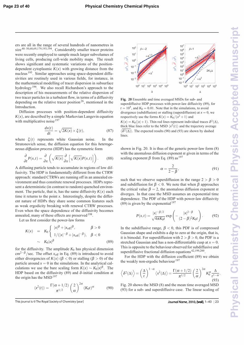
ers are all in the range of several hundreds of nanometres insize48–50,68,69,179,193,194. Considerably smaller tracer proteinswere recently employed to sample much larger subvolumes ofliving cells, producing cell-wide mobility maps. The resultshows significant and systematic variations of the position-dependent cytoplasmic K(x) with growing distance from thenucleus195. Similar approaches using space-dependent diffu-sivities are routinely used in various fields, for instance, inthe mathematical modelling of tracer dispersion in subsurfacehydrology196. We also recall Richardson’s approach to thedescription of his measurements of the relative dispersion oftwo tracer particles in a turbulent flow, in terms of a diffusivitydepending on the relative tracer position26, mentioned in theIntroduction.

Diffusion processes with position-dependent diffusivityK(x), are described by a simple Markovian Langevin equationwith multiplicative noise197

dx(t)dt

=√

2K(x)× ξ (t), (87)

where ξ (t) represents white Gaussian noise. In theStratonovich sense, the diffusion equation for this heteroge-neous diffusion process (HDP) has the symmetric form

∂∂ t

P(x, t) =∂∂x

(√K(x)

∂∂x

[√K(x)P(x, t)

]). (88)

A diffusing particle tends to accumulate in regions of low dif-fusivity. The HDP is fundamentally different from the CTRWapproach: standard CTRWs are running off in an annealed en-vironment and thus constitute renewal processes. HDPs repre-sent a deterministic (in contrast to random) quenched environ-ment. The particle, that is, has the same diffusivity K(x) eachtime it returns to the point x. Interestingly, despite the differ-ent nature of HDPs they share some common features suchas weak ergodicity breaking with renewal CTRW processes.Even when the space dependence of the diffusivity becomesannealed, many of these effects are preserved198.

Let us first consider the power-law forms

K(x) = K0

{ |x|β + |xoff|β , β > 0

1/(|x|−β + |xoff|−β ), β < 0

∼ K0|x|β (89)

for the diffusivity. The amplitude K0 has physical dimensioncm2−β/sec. The offset xoff in Eq. (89) is introduced to avoideither divergencies of K(x) (β < 0) or stalling (β > 0) of theparticle around x = 0 in the simulations. In the analytical cal-culations we use the bare scaling form K(x) ∼ K0|x|β . TheHDP based on the diffusivity (89) and δ -initial condition atthe origin has the MSD197

〈x2(t)〉= Γ(α + 1/2)π1/2

(2α

)2α(K0t)α (90)

��1

��1�2

��2

105104103102101100

102

101

100

10�1

10�2

10�3

�

�x2 �

,Δ2 ,�Δ

2 � ��1

��2

Β�1

2K0�

105104103102101100

107

106

105

104

103

102

101

100

10�1

10�2

�

�x2 �

,Δ2 ,�Δ

2 �

Fig. 20 Ensemble and time averaged MSDs for sub- andsuperdiffusive HDP processes with power-law diffusivity (89), fort = 105, and K0 = 0.01. Note that in the simulations, to avoiddivergence (subdiffusion) or stalling (superdiffusion) at x = 0, werespectively use the forms K(x) = K0/(x2 +1) andK(x) = K0(|x|+1). Thin red lines represent individual traces δ 2(Δ),thick blue lines refer to the MSD 〈x2(t)〉 and the trajectory average〈δ 2(Δ)〉. The expected results (90) and (93) are shown by dashedlines.

shown in Fig. 20. It is thus of the generic power-law form (8)with the anomalous diffusion exponent α given in terms of thescaling exponent β from Eq. (89) as197

α =2

2−β, (91)

such that we observe superdiffusion in the range 2 > β > 0and subdiffusion for β < 0. We note that when β approachesthe critical value β = 2, the anomalous diffusion exponent αdiverges. In that case the MSD assumes an exponential timedependence. The PDF of the HDP with power-law diffusivity(89) is given by the exponential197

P(x, t) =|x|−β/2√

4πK0texp

(− |x|2−β

(2−β )2K0t

). (92)

In the subdiffusive range, β < 0, this PDF is of compressedGaussian shape and exhibits a dip to zero at the origin, that is,it is bimodal. For superdiffusion with 2 > β > 0, the PDF is astretched Gaussian and has a non-differentiable cusp at x = 0.This is opposite to the behaviour observed for subdiffusive andsuperdiffusive fractional diffusion equations42,199,200.

For the HDP with the diffusion coefficient (89) we obtainthe weakly non-ergodic behaviour197

⟨δ 2(Δ)

⟩=

(Δt

)1−α ⟨x2(Δ)

⟩=

Γ(α + 1/2)π1/2

(2α

)2αKα

0Δ

t1−α .

(93)Fig. 20 shows the MSD (8) and the mean time averaged MSD(93) for a sub- and superdiffusive case. The linear scaling of

1–40 | 23

Page 23 of 40 Physical Chemistry Chemical Physics

Phy

sica

lChe

mis

try

Che

mic

alP

hysi

csA

ccep

ted

Man

uscr

ipt

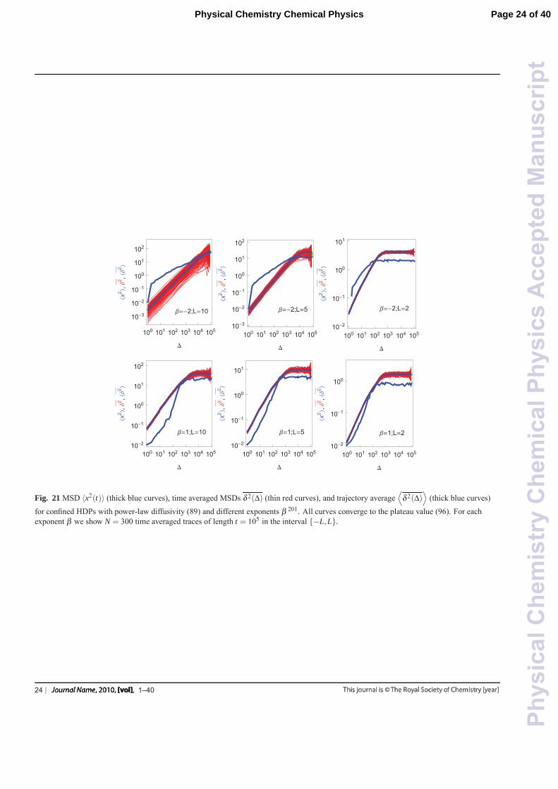
��2;L�10

105104103102101100

102

101

100

10�1

10�2

10�3

�

�x2 �

,Δ2 ,�Δ

2 �

��2;L�5

105104103102101100

102

101

100

10�1

10�2

10�3

�

�x2 �

,Δ2 ,�Δ

2 �

��2;L�2

105104103102101100

101

100

10�1

10�2

�

�x2 �

,Δ2 ,�Δ

2 �

Β�1;L�10

105104103102101100

102

101

100

10�1

10�2

�

�x2 �

,Δ2 ,�Δ

2 �

Β�1;L�5

105104103102101100

101

100

10�1

10�2

�

�x2 �

,Δ2 ,�Δ

2 �

Β�1;L�2

105104103102101100

100

10�1

10�2

�

�x2 �

,Δ2 ,�Δ

2 �

Fig. 21 MSD 〈x2(t)〉 (thick blue curves), time averaged MSDs δ 2(Δ) (thin red curves), and trajectory average⟨

δ 2(Δ)⟩

(thick blue curves)

for confined HDPs with power-law diffusivity (89) and different exponents β 201. All curves converge to the plateau value (96). For eachexponent β we show N = 300 time averaged traces of length t = 105 in the interval {−L,L}.

24 | 1–40

Page 24 of 40Physical Chemistry Chemical Physics

Phy

sica

lChe

mis

try

Che

mic

alP

hysi

csA

ccep

ted

Man

uscr

ipt

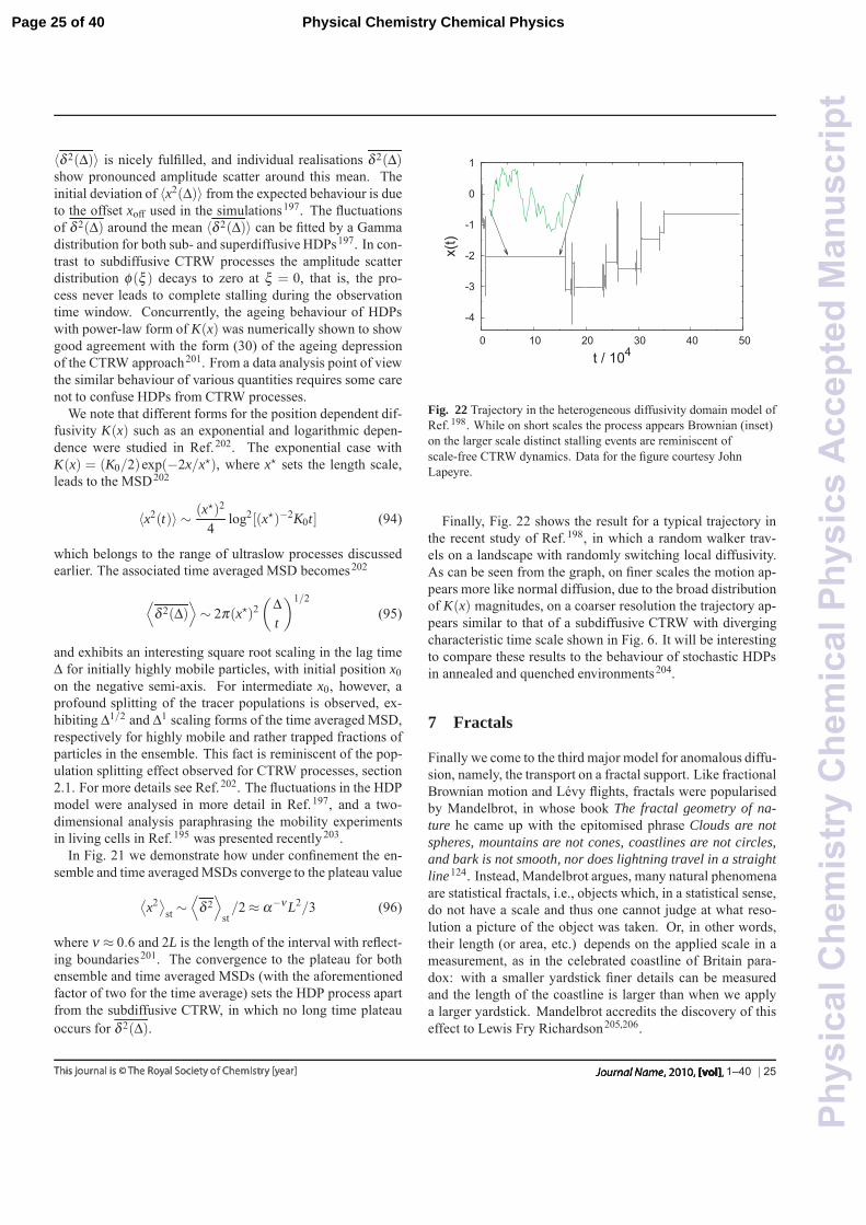
〈δ 2(Δ)〉 is nicely fulfilled, and individual realisations δ 2(Δ)show pronounced amplitude scatter around this mean. Theinitial deviation of 〈x2(Δ)〉 from the expected behaviour is dueto the offset xoff used in the simulations197. The fluctuationsof δ 2(Δ) around the mean 〈δ 2(Δ)〉 can be fitted by a Gammadistribution for both sub- and superdiffusive HDPs197. In con-trast to subdiffusive CTRW processes the amplitude scatterdistribution φ(ξ ) decays to zero at ξ = 0, that is, the pro-cess never leads to complete stalling during the observationtime window. Concurrently, the ageing behaviour of HDPswith power-law form of K(x) was numerically shown to showgood agreement with the form (30) of the ageing depressionof the CTRW approach201. From a data analysis point of viewthe similar behaviour of various quantities requires some carenot to confuse HDPs from CTRW processes.

We note that different forms for the position dependent dif-fusivity K(x) such as an exponential and logarithmic depen-dence were studied in Ref.202. The exponential case withK(x) = (K0/2)exp(−2x/x�), where x� sets the length scale,leads to the MSD202

〈x2(t)〉 ∼ (x�)2

4log2[(x�)−2K0t] (94)

which belongs to the range of ultraslow processes discussedearlier. The associated time averaged MSD becomes202

⟨δ 2(Δ)

⟩∼ 2π(x�)2

(Δt

)1/2(95)

and exhibits an interesting square root scaling in the lag timeΔ for initially highly mobile particles, with initial position x0on the negative semi-axis. For intermediate x0, however, aprofound splitting of the tracer populations is observed, ex-hibiting Δ1/2 and Δ1 scaling forms of the time averaged MSD,respectively for highly mobile and rather trapped fractions ofparticles in the ensemble. This fact is reminiscent of the pop-ulation splitting effect observed for CTRW processes, section2.1. For more details see Ref.202. The fluctuations in the HDPmodel were analysed in more detail in Ref.197, and a two-dimensional analysis paraphrasing the mobility experimentsin living cells in Ref.195 was presented recently203.

In Fig. 21 we demonstrate how under confinement the en-semble and time averaged MSDs converge to the plateau value⟨

x2⟩st ∼

⟨δ 2

⟩st/2 ≈ α−ν L2/3 (96)

where ν ≈ 0.6 and 2L is the length of the interval with reflect-ing boundaries201. The convergence to the plateau for bothensemble and time averaged MSDs (with the aforementionedfactor of two for the time average) sets the HDP process apartfrom the subdiffusive CTRW, in which no long time plateauoccurs for δ 2(Δ).

-4

-3

-2

-1

0

1

0 10 20 30 40 50

x(t)

t / 104

Fig. 22 Trajectory in the heterogeneous diffusivity domain model ofRef. 198. While on short scales the process appears Brownian (inset)on the larger scale distinct stalling events are reminiscent ofscale-free CTRW dynamics. Data for the figure courtesy JohnLapeyre.

Finally, Fig. 22 shows the result for a typical trajectory inthe recent study of Ref.198, in which a random walker trav-els on a landscape with randomly switching local diffusivity.As can be seen from the graph, on finer scales the motion ap-pears more like normal diffusion, due to the broad distributionof K(x) magnitudes, on a coarser resolution the trajectory ap-pears similar to that of a subdiffusive CTRW with divergingcharacteristic time scale shown in Fig. 6. It will be interestingto compare these results to the behaviour of stochastic HDPsin annealed and quenched environments204.

7 Fractals

Finally we come to the third major model for anomalous diffu-sion, namely, the transport on a fractal support. Like fractionalBrownian motion and Levy flights, fractals were popularisedby Mandelbrot, in whose book The fractal geometry of na-ture he came up with the epitomised phrase Clouds are notspheres, mountains are not cones, coastlines are not circles,and bark is not smooth, nor does lightning travel in a straightline124. Instead, Mandelbrot argues, many natural phenomenaare statistical fractals, i.e., objects which, in a statistical sense,do not have a scale and thus one cannot judge at what reso-lution a picture of the object was taken. Or, in other words,their length (or area, etc.) depends on the applied scale in ameasurement, as in the celebrated coastline of Britain para-dox: with a smaller yardstick finer details can be measuredand the length of the coastline is larger than when we applya larger yardstick. Mandelbrot accredits the discovery of thiseffect to Lewis Fry Richardson205,206.

1–40 | 25

Page 25 of 40 Physical Chemistry Chemical Physics

Phy

sica

lChe

mis

try

Che

mic

alP

hysi

csA

ccep

ted

Man

uscr

ipt

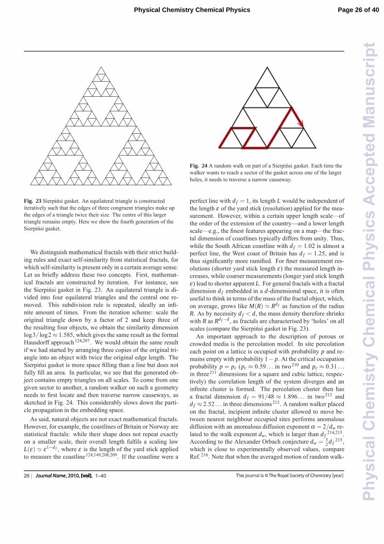
Fig. 23 Sierpinsi gasket. An equilateral triangle is constructediteratively such that the edges of three congruent triangles make upthe edges of a triangle twice their size. The centre of this largertriangle remains empty. Here we show the fourth generation of theSierpinsi gasket.

We distinguish mathematical fractals with their strict build-ing rules and exact self-similarity from statistical fractals, forwhich self-similarity is present only in a certain average sense.Let us briefly address these two concepts. First, mathemat-ical fractals are constructed by iteration. For instance, seethe Sierpinsi gasket in Fig. 23. An equilateral triangle is di-vided into four equilateral triangles and the central one re-moved. This subdivision rule is repeated, ideally an infi-nite amount of times. From the iteration scheme: scale theoriginal triangle down by a factor of 2 and keep three ofthe resulting four objects, we obtain the similarity dimensionlog3/ log2 ≈ 1.585, which gives the same result as the formalHausdorff approach124,207. We would obtain the same resultif we had started by arranging three copies of the original tri-angle into an object with twice the original edge length. TheSierpinsi gasket is more space filling than a line but does notfully fill an area. In particular, we see that the generated ob-ject contains empty triangles on all scales. To come from onegiven sector to another, a random walker on such a geometryneeds to first locate and then traverse narrow causeways, assketched in Fig. 24. This considerably slows down the parti-cle propagation in the embedding space.

As said, natural objects are not exact mathematical fractals.However, for example, the coastlines of Britain or Norway arestatistical fractals: while their shape does not repeat exactlyon a smaller scale, their overall length fulfils a scaling lawL(ε) � ε1−d f , where ε is the length of the yard stick appliedto measure the coastline124,149,208,209. If the coastline were a

Fig. 24 A random walk on part of a Sierpinsi gasket. Each time thewalker wants to reach a sector of the gasket across one of the largerholes, it needs to traverse a narrow causeway.

perfect line with d f = 1, its length L would be independent ofthe length ε of the yard stick (resolution) applied for the mea-surement. However, within a certain upper length scale—ofthe order of the extension of the country—and a lower lengthscale—e.g., the finest features appearing on a map—the frac-tal dimension of coastlines typically differs from unity. Thus,while the South African coastline with d f = 1.02 is almost aperfect line, the West coast of Britain has d f = 1.25, and isthus significantly more ramified. For finer measurement res-olutions (shorter yard stick length ε) the measured length in-creases, while coarser measurements (longer yard stick lengthε) lead to shorter apparent L. For general fractals with a fractaldimension d f embedded in a d-dimensional space, it is oftenuseful to think in terms of the mass of the fractal object, which,on average, grows like M(R) � Rdf as function of the radiusR. As by necessity d f < d, the mass density therefore shrinkswith R as Rdf −d , as fractals are characterised by ‘holes’ on allscales (compare the Sierpinsi gasket in Fig. 23).

An important approach to the description of porous orcrowded media is the percolation model. In site percolationeach point on a lattice is occupied with probability p and re-mains empty with probability 1− p. At the critical occupationprobability p = pc (pc ≈ 0.59 . . . in two210 and pc ≈ 0.31 . . .in three211 dimensions for a square and cubic lattice, respec-tively) the correlation length of the system diverges and aninfinite cluster is formed. The percolation cluster then hasa fractal dimension d f = 91/48 ≈ 1.896 . . . in two212 andd f ≈ 2.52 . . . in three dimensions213. A random walker placedon the fractal, incipient infinite cluster allowed to move be-tween nearest neighbour occupied sites performs anomalousdiffusion with an anomalous diffusion exponent α = 2/dw re-lated to the walk exponent dw, which is larger than d f

214,215.According to the Alexander Orbach conjecture dw = 3

2d f215,

which is close to experimentally observed values, compareRef.216. Note that when the averaged motion of random walk-

26 | 1–40

Page 26 of 40Physical Chemistry Chemical Physics

Phy

sica

lChe

mis

try

Che

mic

alP

hysi

csA

ccep

ted

Man

uscr

ipt

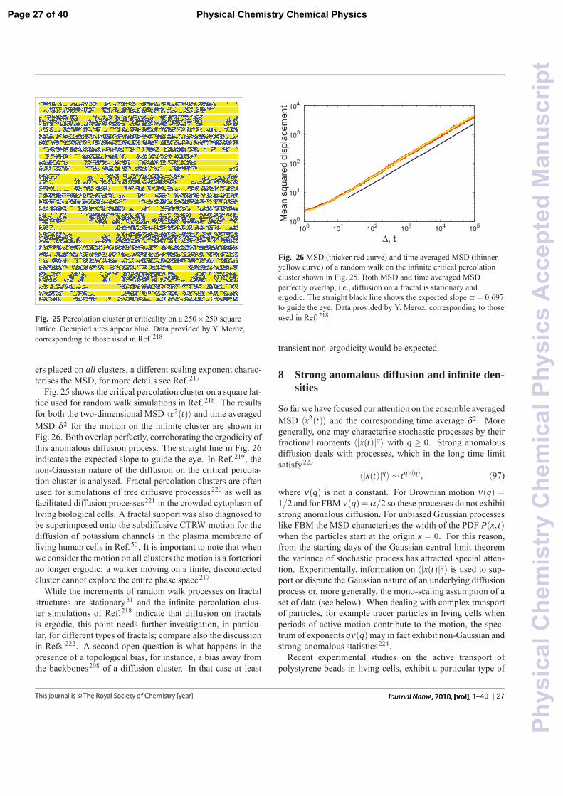
Fig. 25 Percolation cluster at criticality on a 250×250 squarelattice. Occupied sites appear blue. Data provided by Y. Meroz,corresponding to those used in Ref. 218.

ers placed on all clusters, a different scaling exponent charac-terises the MSD, for more details see Ref.217.

Fig. 25 shows the critical percolation cluster on a square lat-tice used for random walk simulations in Ref.218. The resultsfor both the two-dimensional MSD 〈r2(t)〉 and time averagedMSD δ 2 for the motion on the infinite cluster are shown inFig. 26. Both overlap perfectly, corroborating the ergodicity ofthis anomalous diffusion process. The straight line in Fig. 26indicates the expected slope to guide the eye. In Ref.219, thenon-Gaussian nature of the diffusion on the critical percola-tion cluster is analysed. Fractal percolation clusters are oftenused for simulations of free diffusive processes220 as well asfacilitated diffusion processes221 in the crowded cytoplasm ofliving biological cells. A fractal support was also diagnosed tobe superimposed onto the subdiffusive CTRW motion for thediffusion of potassium channels in the plasma membrane ofliving human cells in Ref.50. It is important to note that whenwe consider the motion on all clusters the motion is a forteriorino longer ergodic: a walker moving on a finite, disconnectedcluster cannot explore the entire phase space217.

While the increments of random walk processes on fractalstructures are stationary31 and the infinite percolation clus-ter simulations of Ref.218 indicate that diffusion on fractalsis ergodic, this point needs further investigation, in particu-lar, for different types of fractals; compare also the discussionin Refs.222. A second open question is what happens in thepresence of a topological bias, for instance, a bias away fromthe backbones208 of a diffusion cluster. In that case at least

100

101

102

103

104

100 101 102 103 104 105

Mea

n sq

uare

d di

spla

cem

ent

Δ, t

Fig. 26 MSD (thicker red curve) and time averaged MSD (thinneryellow curve) of a random walk on the infinite critical percolationcluster shown in Fig. 25. Both MSD and time averaged MSDperfectly overlap, i.e., diffusion on a fractal is stationary andergodic. The straight black line shows the expected slope α = 0.697to guide the eye. Data provided by Y. Meroz, corresponding to thoseused in Ref. 218.

transient non-ergodicity would be expected.

8 Strong anomalous diffusion and infinite den-sities

So far we have focused our attention on the ensemble averagedMSD 〈x2(t)〉 and the corresponding time average δ 2. Moregenerally, one may characterise stochastic processes by theirfractional moments 〈|x(t)|q〉 with q ≥ 0. Strong anomalousdiffusion deals with processes, which in the long time limitsatisfy223

〈|x(t)|q〉 ∼ tqν(q), (97)

where ν(q) is not a constant. For Brownian motion ν(q) =1/2 and for FBM ν(q)=α/2 so these processes do not exhibitstrong anomalous diffusion. For unbiased Gaussian processeslike FBM the MSD characterises the width of the PDF P(x, t)when the particles start at the origin x = 0. For this reason,from the starting days of the Gaussian central limit theoremthe variance of stochastic process has attracted special atten-tion. Experimentally, information on 〈|x(t)|q〉 is used to sup-port or dispute the Gaussian nature of an underlying diffusionprocess or, more generally, the mono-scaling assumption of aset of data (see below). When dealing with complex transportof particles, for example tracer particles in living cells whenperiods of active motion contribute to the motion, the spec-trum of exponents qν(q) may in fact exhibit non-Gaussian andstrong-anomalous statistics224.

Recent experimental studies on the active transport ofpolystyrene beads in living cells, exhibit a particular type of

1–40 | 27

Page 27 of 40 Physical Chemistry Chemical Physics

Phy

sica

lChe

mis

try

Che

mic

alP

hysi

csA

ccep

ted

Man

uscr

ipt

strong anomalous diffusion. The data analysis exhibits piece-wise linear behaviour with

qν(q) =

{μq, q < qc

aq− b, q > qc(98)

with the positive constants qc, μ , a, and b. Such a behaviouris sometimes called bi-fractal scaling, as the simplest caseof multi-fractal behaviour. More importantly this bi-linearbehaviour is widespread and found in many models of non-linear dynamics223,225–229, transport in optical lattices230,231,models of transport in disordered Levy glasses232–234, andother stochastic models88,235,236. The parameters qc, μ , a,and b are non-universal and hence give specific informationon the underlying model or process. As emphasised by Vulpi-ani and coworkers223 strong anomalous diffusion implies thebreakdown of mono-scaling theories which predict P(x, t) ∼t−ν f (x/tν ) in terms of a scaling function f (·). For exam-ple, FBM, FLE, sub-diffusive decoupled CTRW, and frac-tional diffusion equations42,56 do not predict the piecewise bi-linear scaling (98) of the moments, in other words these pop-ular stochastic models considered above cannot describe theactive transport found in Ref.224. In experiments a � 0.8 (seediscussion below).

Roughly speaking, the piecewise linear scaling of the spec-trum qν(q) implies that lower order moments q < qc still fol-low a diffusive, possibly anomalous process if μ �= 1, while thelinear increase of the spectrum qν(q) ∼ q for q � 1 impliesa ballistic scaling, since if x scales like t, 〈|x|q〉 scales withtq. This implies that the process is actually a mixture of botha diffusive process x ∝ tμ and a ballistic element x ∝ t, andhence characterising the process as an anomalous diffusionprocess is in some sense misleading. In particular, we shouldnot universally accept the special role of the second moment,beyond the fact that it indicates certain deviations from nor-mal behaviour. A typical situation occurs when P(x, t) forsmall x scales diffusively (ν = 1/2), however, for certain largex the scaling becomes ballistic (ν = 1). Here we focus onone stochastic model of strong anomalous diffusion, the Levywalk model mentioned in section 3.5. For more details on themathematical treatment of the following, see Ref.237.

Levy walks represent a widely applicable model describ-ing superdiffusion51,81,238–244. In its simplest one dimensionalversion, a particle starts at the origin at time t = 0, and travelswith velocity v1, drawn from the PDF F(v). The duration ofthe travelling event is τ1 which is drawn from the PDF ψ(τ).The position of the particle at time τ1 is x = v1τ1. The pro-cess is then renewed, until time t is reached: a new velocity v2and waiting time τ2 are independently drawn from F(v) andψ(τ), and this process is repeated. The position of the particleis then simply x(t) =

∫ t0 v(t)dt. If the PDF ψ(τ) of the flight

duration is exponential and the velocity distribution Gaussian

with zero mean, we recover the famous Drude model245. Er-godic properties of Levy walks were analysed in Refs.136–138,see also section 2.5.

We assume that the velocity PDF is symmetric—F(v) =F(−v), such that 〈v〉= 0—and that all moments of F(v) are fi-nite, for instance, a Gaussian PDF. The main ingredient of thestochastic model are the power-law distributed waiting times(14). These can be justified from first principle models orfrom observations, at least in some systems, compare the dis-cussions in Refs.39,51,241. We here limit our discussion to thecase 1 < α < 2 which in turn implies that the average sojourntime 〈τ〉 is finite, however, its variance diverges. Rather gen-erally, it is easy to understand that the MSD is bounded by〈x2(t)〉 ≤ 〈v2〉t2. Roughly speaking, the ith jump in the pro-cess is given by δxi = viτi, and due to the assumed power-lawPDF of waiting times the PDF of this increment is a symmet-ric distribution (due to the symmetry of the distribution of v)with long tails

λ (δx) ∝ |δx|−1−α . (99)

The typical number of jumps in the process is N � t/〈τ〉.Hence a hand-waving argument yields the PDF of the posi-tion of the particle using the generalised central limit theorem.Namely, x � ∑N=t/〈τ〉

i=1 δxi with the variance of δxi being infi-nite, such that we expect that the PDF of particles is given by(in dimensionless units)

P(x, t)� 1t1/α Lα ,0

( xt1/α

). (100)

Here Lα ,0(x) is the symmetric Levy distribution, whoseFourier pair is exp(−|k|α), such that the case α = 2 corre-sponds to a Gaussian process. Taken seriously, this centrallimit theorem implies

〈|x|q〉 ∼{

tq/α , q < α

∞, q > α.(101)

These hand-waving arguments provide the correct scaling ofthe lower order moments, however, the results for higher ordermoments, including the second moment, are obviously wrong:the particle cannot travel faster than ballistic motion.† Our ar-gument is flawed since we have neglected the correlation be-tween the jump sized and time in the problem. A more precisemathematical analysis leads to the result237

〈|x|q〉 ∼{

tq/α , q < α

tq+1−α , q > α(102)

In terms of the parameters introduced in Eq. (98), we thusidentify μ = 1/α , qc = α , a = 1, and b = α − 1. We see that

† As we required all moments of the velocity distribution F(v) to be finite, wehave a kind of light cone beyond which the particle cannot be found.

28 | 1–40

Page 28 of 40Physical Chemistry Chemical Physics

Phy

sica

lChe

mis

try

Che

mic

alP

hysi

csA

ccep

ted

Man

uscr

ipt

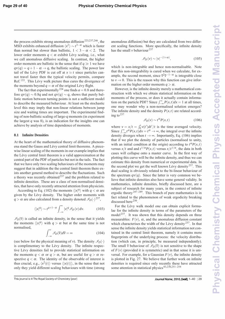
the process exhibits strong anomalous diffusion223,237,246, theMSD exhibits enhanced diffusion 〈x2〉 ∼ t3−α which is fasterthan normal but slower than ballistic, 1 < 3− α < 2. Thelower order moments q < α exhibit Levy scaling, i.e., whatwe call anomalous diffusive scaling. In contrast, the higherorder moments are ballistic in the sense that if q � 1 we haveqν(q) = q+ 1−α → q, the ballistic scaling. The power lawtail of the Levy PDF is cut off at x � t since particles can-not travel faster then the typical velocity permits, compareRef.133. This Levy walk picture thus cures the divergence ofthe moments beyond q = α of the original Levy flight.

The fact that experimentally224 one finds a= 0.8 and there-fore qν(q) ∼ 0.8q and not qν(q) ∼ q, shows that purely bal-listic motion between turning points is not a sufficient modelto describe the measured behaviour. At least on the stochasticlevel this may imply that non-linear relations between jumpsize and waiting times are important. The experimental find-ing of non-ballistic scaling of large-q moments (in experimentthe largest q was 8), is an indication for the insights one canachieve by analysis of time dependence of moments.

8.1 Infinite Densities

At the heart of the mathematical theory of diffusive phenom-ena stand the Gauss and Levy central limit theorems. A piece-wise linear scaling of the moments in our example implies thatthe Levy central limit theorem is a valid approximation at thecentral part of the PDF of particles but not in the tails. The factthat we have only two scaling behaviours of the moments maysuggest that in addition the the central limit theorem there ex-ists another general method to describe the fluctuations. Sucha theory was recently obtained237 and the problem related toinfinite densities. These are a class of non-normalised densi-ties, that have only recently attracted attention from physicists.

According to Eq. (102) the moments 〈|x|q〉 with q < α aregiven by the Levy density. The higher order moments withq > α are also calculated from a density denoted ID(·)237,

〈|x|q〉 ∼ tq+1−α∫ ∞

−∞|v|qID (v)dv. (103)

ID(v) is called an infinite density, in the sense that it yieldsthe moments 〈|x|q〉 with q > α but at the same time is notnormalised, ∫ ∞

−∞ID(v)dv = ∞ (104)

(see below for the physical meaning of v). The density ID(·)is complimentary to the Levy density. The infinite respec-tive Levy densities fail to provide statistical information onthe moments q < α or q > α , but are useful for q > α re-spective q < α . The identity of the observable of interest isthus crucial, e.g., 〈x2(t)〉 versus 〈|x(t)|〉, in the sense that notonly they yield different scaling behaviours with time (strong

anomalous diffusion) but they are calculated from two differ-ent scaling functions. More specifically, the infinite densityhas the small v behaviour237

ID (v)∼ |v|−(1+α), (105)

which is non-integrable and hence non-normalisable. Notethat this non-integrability is cured when we calculate, for ex-ample, the second moment, since v2v−1−α is integrable closeto v → 0. This is the reason why this function can give infor-mation on the higher order moments q > α .

However, is the infinite density merely a mathematical con-struction with which we obtain statistical information on themoments of the process, or does it actually contain informa-tion on the particle PDF? Since

∫ ∞−∞ P(x, t)dx = 1 at all times,

one may wonder why a non-normalised solution emerges?The infinite density and the density P(x, t) are related accord-ing to237

ID(v)∼ tαP(x, t) (106)

where v = x/t =∫ t

0 v(t ′)dt ′/t is the time averaged velocity.Since

∫ ∞−∞ tαP(x, t)dx = tα → ∞, the integral over the infinite

density diverges when t → ∞. Importantly, Eq. (106) impliesthat if we plot the density of particles (normalised to unity,with an initial condition at the origin) according to tαP(x, t)versus x/t and and t1/αP(x, t) versus x/t1/α , the data in bothcases will collapse onto a master curve. In the first way ofplotting this curve will be the infinite density, and thus we canestimate this density from numerical or experimental data. Inthe second plot we get the well known Levy density237. Thisdual scaling is obviously related to the bi-linear behaviour ofthe spectrum qν(q). Since the latter is very common we be-lieve that infinite densities also have some general validity. Inmathematics, infinite densities, briefly discussed here, are asubject of research for many years, in the context of infiniteergodic theory247–249. This branch of pure mathematics is infact related to the phenomenon of weak ergodicity breakingdiscussed here250.

For the Levy walk model one can obtain explicit formu-lae for the infinite density in terms of the parameters of themodel237. It was shown that this density depends on threemeasurables: F(v), α , and the anomalous diffusion constantwhich characterises the width of the Levy density237. In thatsense the infinite density yields statistical information not con-tained in the central limit theorem, namely it contains morefingerprints of the underlying process: the velocity distribu-tion (which can, in principle, be measured independently).The small v behaviour of ID(v) is not sensitive to the shapeof F(v) (provided it is symmetric) and in that sense it is uni-versal. For example, for a Gaussian F(v), the infinite densityis plotted in Fig. 27. We believe that further work on infinitedensities is required since only recently these have attractedsome attention in statistical physics83,230,251–254

1–40 | 29

Page 29 of 40 Physical Chemistry Chemical Physics

Phy

sica

lChe

mis

try

Che

mic

alP

hysi

csA

ccep

ted

Man

uscr

ipt

−5 0 510−10

10−5

100

105

v

I D(v)

α = 1.2α = 1.5α = 1.8

Fig. 27 Infinite density for a Gaussian velocity distribution F(v).Notice the divergence of the density at the origin. This divergence isnon-integrable, hence these functions are non-normalisable. Still,they describe the statistical properties of physical particles237.

9 Measurables

Normal and anomalous diffusion are key to many biologicalsignalling processes and a vast number of biochemical reac-tions in cells, or to the spreading dynamics in inanimate com-plex systems. To be able to analyse diffusion measurementin a physical meaningful way and to make predictions forsecondary processes such as reaction rates or signalling cas-cades, it is absolutely necessary to know the exact nature of thestochastic process driving the particle motion. For instance,the first passage behaviour is vastly different between the pro-cesses reviewed here. In this section we describe some exper-imentally relevant observables whose complementary charac-ter enables one to attain a fair degree of certainty that a givenset of data are based on a concrete stochastic process. Analy-ses based on the application of different measures are, for in-stance, presented in Refs.44,50,68,69,175,176,255–260. As demon-strated in literature50,68,69,72, we note that there is a priori nogood reason to assume that in a complex systems a singleone of the above processes is sufficient to adequately describeall the observed dynamic features: sometimes it is necessaryto combine at least two of the processes, that may influencethe particle motion simultaneously or at different time scales.When passive diffusion is combined with intermittent activemotion additional challenges to the data analysis arise261.

MSD

The MSD is unarguably the most common way to analysestochastic data. Depending on the kind of measurement thequantity to evaluate is the MSD 〈x2(t)〉 or the time averagedMSD δ 2(Δ). The latter is the typical approach to the analy-

sis of the time series obtained from single particle tracking.If the time averaged MSD exhibits anomalous scaling of theform δ 2(Δ) � Δα and δ 2(Δ) = 〈x2(Δ)〉 we are dealing withan (asymptotically) ergodic process, and when we want to usethe data to identify the underlying stochastic process we canalready eliminate CTRW motion and diffusion processes withtime or space dependent diffusivity as sole contributions. Tobe more specific, additional complementary measures need tobe evaluated.

Scatter of time averages

The statistics of the scatter of the amplitude δ 2(Δ) of thetime averaged MSD for a set of individual trajectories at agiven lag time Δ is a useful indicator for the classificationof the anomalous diffusion process. We quantify this scat-ter by the distribution φ(ξ ) of the dimensionless amplitudeξ = δ 2(Δ)/

⟨δ 2(Δ)

⟩and by its variance, the ergodicity break-

ing parameter EB = 〈ξ 2〉− 〈ξ 〉2 introduced earlier. As a gen-eral trend the fluctuations increase for any type of motionwhen the lag time is taken too large in comparison to themeasurement time t. We note that due to the very definition(6) of the time averaged MSD the plateau value observed forsome of the processes under confinement is twice the value ofthe MSD. When the lag time approaches t, the time averagedMSD δ 2 shows a cusp to the thermal value 〈x2〉th, as shownexplicitly for the SBM model in Ref.189.

For Brownian motion the PDF φ(ξ ) converges to the sharpform φ(ξ )→ δ (ξ − 1) around the ergodic value ξ = 1 in thelong time limit t → ∞. At finite t this δ -peak broadens. Indi-vidual trajectories exhibit erratic fluctuations of δ 2 as Δ → t.The ergodicity breaking parameter tends to zero with the ratioΔ/t in the form EB = 4

3 Δ/t.For subdiffusive CTRW motion the trajectory-to-trajectory

fluctuations are asymptotic, that is, the ergodicity breakingparameter has the finite limiting value (25) varying with αbetween unity and zero. As in this process the fluctuationsare statistically given by the number of jumps performed dur-ing its time evolution73, the PDF φ(ξ ) remains unchangedwhen the process becomes confined. The distribution φ(ξ )has a finite value at ξ = 0 for any given Δ, a strong charac-teristic of the weakly non-ergodic CTRW motion. For agedCTRW processes φ(ξ ) has a discrete immobile contributionproportional to δ (ξ ) and a continuum part whose distributionis qualitatively similar to the non-aged process, albeit thereoccurs a redistribution of this continuous part to larger ξ val-ues73. The PDF φ(ξ ) for noisy CTRW processes with su-perimposed Ornstein-Uhlenbeck or Brownian noise narrowsdown for increasing noise strength98. Finally, we note thatsubdiffusive CTRW processes with a cutoff of the power-lawwaiting time distribution exhibit an MSD with all features of

30 | 1–40

Page 30 of 40Physical Chemistry Chemical Physics

Phy

sica

lChe

mis

try

Che

mic

alP

hysi

csA

ccep

ted

Man

uscr

ipt

the process with diverging waiting time scale roughly up tothe cutoff time, however, due to the lack of extreme waitingevents the scatter distribution φ(ξ ) appears significantly moreergodic68, compare also the discussion in Ref.262,263.

For FBM and FLE motion the scatter distribution at suf-ficiently short lag times is Gaussian and becomes somewhatasymmetric but preserves the property φ(0) = 0 for largerΔ158. The ergodicity breaking parameter tends to zero with theratio Δ/t 156. For the transiently non-ergodic behaviour underconfinement see Ref.166,179. In general, the scatter distribu-tion and the ergodicity breaking parameter of both processesare relatively similar to those of regular Brownian motion.

SBM was shown to be a weakly non-ergodic process butits ergodicity breaking parameter tends to zero with the ratioΔ/t 189,190. The PDF φ(ξ ) is approximately bell-shaped albeitwider than for the corresponding FBM with identical anoma-lous diffusion exponent α .

For HDPs the form of the PDF φ(ξ ) follows an asymmet-ric Rayleigh-like or generalised Gamma distribution197. Thewidth of φ(ξ ) for HDPs with power-law form (89) grows fromthe minimal Brownian value attained for the scaling exponentβ = 0 of K(x) and diverges at the critical point β → 2. Forconfined HDPs the width of φ(ξ ) decreases drastically for allβ values, often reaching only a minute scatter. The ergodicitybreaking parameter tends to zero as 1/t for fixed Δ201.

We note that in some cases, in lieu of the ergodicity break-ing parameter defined above—which represents a sufficientcondition for (non-)ergodicity—oneuses the parameter E B =⟨

δ 2(Δ)⟩/⟨x2(Δ)

⟩138, representing a necessary condition forergodicity.

First passage time statistics

When sufficient statistics are available one may use the firstpassage time statistics to distinguish different kinds of anoma-lous diffusion processes. In single particle tracking experi-ments the first passage can simply be measured as the mo-ments in time when the tracer passes a certain distance fromits original point of release. As shown in Ref.264 the scalingof the mean first passage time obtained from a statistical num-ber of repeats of such an experiment with the distance fromthe origin may be a good indicator for the underlying diffu-sion process. Moreover, the PDF of first passage times can bea good indicator, especially for confined systems. While sub-diffusive CTRW processes with their scale-free waiting timesstill exhibit a power-law decay under confinement42,94, otherprocesses have an exponential form of the first passage PDF.For semi-open intervals, we note that the dependence of thescaling exponent for the first passage PDF on the stochas-tic process may either be increasing or decreasing‡ with the

‡ Notably, this occurs for FBM 154,155.

anomalous diffusion exponent α , and could thus also serve asan indicator when α is varied.

Mean maximal excursions and higher order moments

Apart from the regular PDF P(x, t) a stochastic process maybe characterised by another, related quantity, the PDF of themaximal excursion. This PDF measures the likelihood that atsome time t after its initial release at the origin, the particlehas not travelled farther than the distance x256,265. This dis-tribution may be reconstructed from the measured single par-ticle traces, and then higher order moments calculated fromthe data. For CTRW and FBM the scaling behaviour of thesecond moment of the mean maximal excursion as well as thefourth moments are known. It can be shown that the ratios ofthe regular moments 〈x4〉/〈x2〉2 and the corresponding quan-tities of the mean maximal excursions obey certain inequali-ties256. The behaviour of the other processes with respect tothis method remain to be analysed. However, we mention thatthe method of the mean maximal excursion has a clear advan-tage over the regular PDF as the mean maximal excursion dy-namics is less dispersed and the associated moments thereforemore reliable for finite data sets256.

Distribution of local diffusivity

An interesting tool to analyse single particle tracking data is tomeasure the distribution of the local anomalous diffusion coef-ficient as function of the (lag) time from the ratio of the MSD(time averaged MSD) versus the (lag) time to some positivepower. These distributions for a weakly non-ergodic processare different according to whether the MSD or the time aver-aged MSD are evaluated. A detailed discussion for Brown-ian processes with spatially varying diffusivity and for CTRWprocesses can be found in Refs.266,267. This method still needsto be analysed for the other anomalous stochastic processesconsidered herein.

Non-Gaussianity measure

Similar to the ergodicity breaking parameter EB, the non-Gaussianity measure G involves higher order moments. Interms of the experimentally relevant time averaged MSD wedefine the non-Gaussianity as217

G(Δ) =d

d+ 2×

⟨δ 4(Δ)

⟩⟨

δ 2(Δ)⟩2 − 1, (107)

in dimension d, where the fourth time averaged moment isdefined via

δ 4(Δ) =1

t −Δ

∫ t−Δ

0

(x(t ′+Δ)− x(t ′)

)4dt ′. (108)

1–40 | 31

Page 31 of 40 Physical Chemistry Chemical Physics

Phy

sica

lChe

mis

try

Che

mic

alP

hysi

csA

ccep

ted

Man

uscr

ipt

For Brownian motion G = 0, while this parameter deviatesfrom zero for progressively non-Brownian diffusion. Thevalue of G provides a sensitive measure for the type of dif-fusion process under consideration. For instance, based on Gmeasurements for diffusion of fluorescent nanobeads in com-plex crowded fluids, the Gaussian FBM-like process was re-cently proposed as suitable mathematical model rather thanCTRW process268.

The p-variation method

The p-variation method is based on the evaluation of the pthpower of a partial sum of increments of a given stochastic pro-cess177,269. It was applied as a measure to distinguish the non-Gaussian subdiffusive CTRW from the Gaussian FBM pro-cess177,269. An attractive feature of the p-variation test is itsapplicability to both unbounded and confined systems, evenwhen based on a single sufficiently long experimental trace.When the recorded time traces are affected by a highly noisyenvironment, the p-variation test may become inconclusive98.

Velocity auto correlation

The experimentally accessible correlation of increments alongsome time trace x(t) can be probed in terms of the covari-ance44

C(ε)ν (τ) = ε−2

⟨(x(τ + ε)− x(τ))(x(ε)− x(0)

)⟩. (109)

Although it is based on increments of the position rather thanon the real velocity of the particle, the quantity (109) is of-ten referred to as the velocity auto-correlation function ofthe process x(t). For free, unconfined CTRW processes thisfunction drops to zero algebraically as C(ε)

ν (τ) ∼ 1− (τ/ε)α

and vanishes at τ > ε due to the independence of succes-sive steps44. With this property CTRW motion is easily dis-tinguishable from unconfined FBM, the latter being charac-terised by a crossover to negative values (a signature of theantipersistence) and a power-law recovery back to zero. Theautocorrelation can be successfully used to analyse the natureof an anomalous diffusion processes166,197. However, for con-fined motion also the CTRW process exhibits some form ofantipersistence due to the reflections at the boundaries or therising flanks of the confining potential. In that case the be-haviour of the function C(ε)

ν (τ) becomes empirically indistin-guishable between confined CTRW and FBM44.

10 Discussion and conclusions

Brownian diffusion with its Gaussian propagator has an ap-pealing beauty in its universality. No matter what the exactdetails of the underlying process are, the limiting behaviour is

completely determined by the MSD and its linear growth withtime. Concurrently, it is ergodic, so all quantities measuredas time averages of sufficiently long single trajectories can besafely interpreted in terms of the readily available ensembleaverages. At the same time one could also perceive Brown-ian diffusion as somewhat too restrictive: many experimentalobservation are much richer and cannot be explained by theGaussian propagator emanating from the central limit theo-rem. We note that while it may be true that apparent anoma-lous diffusion may in fact be due to transient crossovers ofBrownian motion in confined geometries270–274 the oppositemay also be true: some diffusion processes filed under Brow-nian motion may in reality be anomalous64. One of the rea-sons may be the weakly non-ergodic behaviour discussed inthis review.

Especially since more refined measurement techniques suchas space resolved fluorescence recovery after photobleachingmeasurements and, in particular, high resolution single parti-cle tracking have become available, anomalous diffusion hasbeen widely observed. Most importantly, information be-yond the time scaling of the MSD can be extracted from thedata. These observations demonstrate that in different sys-tems anomalous diffusion has different diffusive, first pas-sage, and ergodic characteristics. In particular, disparities be-tween ensemble and time averaged observables have been re-ported. Accommodating the features of anomalous diffusionand non-ergodicity poses the challenge to come up with a plu-ralistic range of stochastic models for the description of non-Brownian diffusion processes.

We here summarised the state of the art in the study of theproperties of the most popular anomalous diffusion processes.In view of their importance in the analysis of experimental orsimulations data we paid specific attention to the time and en-semble averaged MSDs. For ergodic processes both quantitiesare identical for sufficiently long measurements and ensem-bles. In the opposite case, when time and ensemble averagedMSDs are asymptotically disparate, we speak of a weaklynon-ergodic process. The rich range of behaviours are listedin Table 1. In the sense of the ensemble averaged MSD, theconsidered models span from cubic time scaling down to ul-traslow, logarithmic time evolution. Considering the lag timedependence of the time averaged MSD, the variation is muchnarrower, from quadratic scaling to a square root dependence.In most weakly non-ergodic cases a linear lag time depen-dence is observed and may be falsely interpreted as normaldiffusion.

From a statistical physics point of view the variety of be-haviours listed in Table 1 poses a number of questions, inparticular, for a classification scheme of anomalous diffusionprocesses with respect to their (non-)ergodic behaviour andhow fundamental mathematical concepts have to be gener-alised, for instance, the Khinchin theorem45. Moreover, it is

32 | 1–40

Page 32 of 40Physical Chemistry Chemical Physics

Phy

sica

lChe

mis

try

Che

mic

alP

hysi

csA

ccep

ted

Man

uscr

ipt

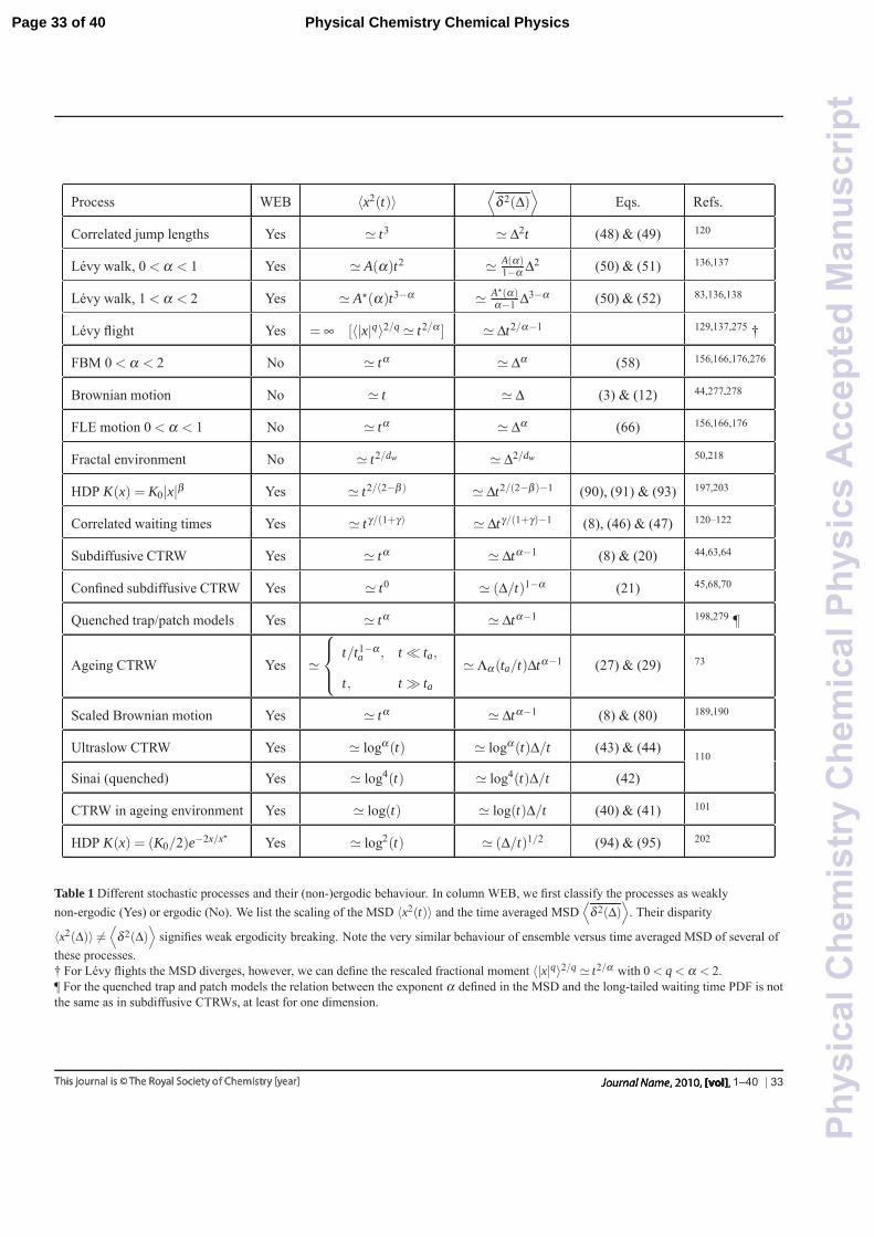
Process WEB 〈x2(t)〉⟨

δ 2(Δ)⟩

Eqs. Refs.

Correlated jump lengths Yes � t3 � Δ2t (48) & (49) 120

Levy walk, 0 < α < 1 Yes � A(α)t2 � A(α)1−α Δ2 (50) & (51) 136,137

Levy walk, 1 < α < 2 Yes � A�(α)t3−α � A�(α)α−1 Δ3−α (50) & (52) 83,136,138

Levy flight Yes = ∞ [〈|x|q〉2/q � t2/α ] � Δt2/α−1 129,137,275 †

FBM 0 < α < 2 No � tα � Δα (58) 156,166,176,276

Brownian motion No � t � Δ (3) & (12) 44,277,278

FLE motion 0 < α < 1 No � tα � Δα (66) 156,166,176

Fractal environment No � t2/dw � Δ2/dw 50,218

HDP K(x) = K0|x|β Yes � t2/(2−β ) � Δt2/(2−β )−1 (90), (91) & (93) 197,203

Correlated waiting times Yes � tγ/(1+γ) � Δtγ/(1+γ)−1 (8), (46) & (47) 120–122

Subdiffusive CTRW Yes � tα � Δtα−1 (8) & (20) 44,63,64

Confined subdiffusive CTRW Yes � t0 � (Δ/t)1−α (21) 45,68,70

Quenched trap/patch models Yes � tα � Δtα−1 198,279 ¶

Ageing CTRW Yes �

⎧⎪⎨⎪⎩ t/t1−αa , t � ta,

t, t � ta� Λα(ta/t)Δtα−1 (27) & (29) 73

Scaled Brownian motion Yes � tα � Δtα−1 (8) & (80) 189,190

Ultraslow CTRW Yes � logα(t) � logα(t)Δ/t (43) & (44)110

Sinai (quenched) Yes � log4(t) � log4(t)Δ/t (42)

CTRW in ageing environment Yes � log(t) � log(t)Δ/t (40) & (41) 101

HDP K(x) = (K0/2)e−2x/x� Yes � log2(t) � (Δ/t)1/2 (94) & (95) 202

Table 1 Different stochastic processes and their (non-)ergodic behaviour. In column WEB, we first classify the processes as weaklynon-ergodic (Yes) or ergodic (No). We list the scaling of the MSD 〈x2(t)〉 and the time averaged MSD

⟨δ 2(Δ)

⟩. Their disparity

〈x2(Δ)〉 �=⟨

δ 2(Δ)⟩

signifies weak ergodicity breaking. Note the very similar behaviour of ensemble versus time averaged MSD of several ofthese processes.† For Levy flights the MSD diverges, however, we can define the rescaled fractional moment 〈|x|q〉2/q � t2/α with 0 < q < α < 2.¶ For the quenched trap and patch models the relation between the exponent α defined in the MSD and the long-tailed waiting time PDF is notthe same as in subdiffusive CTRWs, at least for one dimension.

1–40 | 33

Page 33 of 40 Physical Chemistry Chemical Physics

Phy

sica

lChe

mis

try

Che

mic

alP

hysi

csA

ccep

ted

Man

uscr

ipt

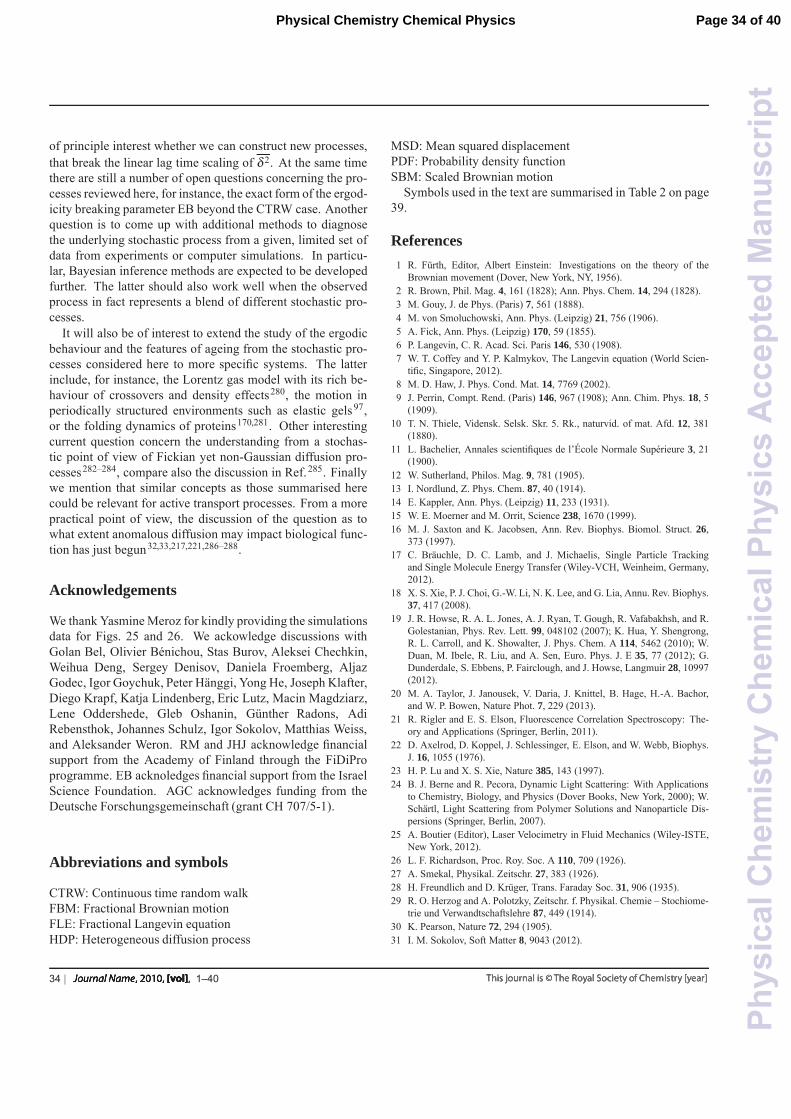
of principle interest whether we can construct new processes,that break the linear lag time scaling of δ 2. At the same timethere are still a number of open questions concerning the pro-cesses reviewed here, for instance, the exact form of the ergod-icity breaking parameter EB beyond the CTRW case. Anotherquestion is to come up with additional methods to diagnosethe underlying stochastic process from a given, limited set ofdata from experiments or computer simulations. In particu-lar, Bayesian inference methods are expected to be developedfurther. The latter should also work well when the observedprocess in fact represents a blend of different stochastic pro-cesses.

It will also be of interest to extend the study of the ergodicbehaviour and the features of ageing from the stochastic pro-cesses considered here to more specific systems. The latterinclude, for instance, the Lorentz gas model with its rich be-haviour of crossovers and density effects280, the motion inperiodically structured environments such as elastic gels97,or the folding dynamics of proteins170,281. Other interestingcurrent question concern the understanding from a stochas-tic point of view of Fickian yet non-Gaussian diffusion pro-cesses282–284, compare also the discussion in Ref.285. Finallywe mention that similar concepts as those summarised herecould be relevant for active transport processes. From a morepractical point of view, the discussion of the question as towhat extent anomalous diffusion may impact biological func-tion has just begun32,33,217,221,286–288.

Acknowledgements

We thank Yasmine Meroz for kindly providing the simulationsdata for Figs. 25 and 26. We ackowledge discussions withGolan Bel, Olivier Benichou, Stas Burov, Aleksei Chechkin,Weihua Deng, Sergey Denisov, Daniela Froemberg, AljazGodec, Igor Goychuk, Peter Hanggi, Yong He, Joseph Klafter,Diego Krapf, Katja Lindenberg, Eric Lutz, Macin Magdziarz,Lene Oddershede, Gleb Oshanin, Gunther Radons, AdiRebensthok, Johannes Schulz, Igor Sokolov, Matthias Weiss,and Aleksander Weron. RM and JHJ acknowledge financialsupport from the Academy of Finland through the FiDiProprogramme. EB acknoledges financial support from the IsraelScience Foundation. AGC acknowledges funding from theDeutsche Forschungsgemeinschaft (grant CH 707/5-1).

Abbreviations and symbols

CTRW: Continuous time random walkFBM: Fractional Brownian motionFLE: Fractional Langevin equationHDP: Heterogeneous diffusion process

MSD: Mean squared displacementPDF: Probability density functionSBM: Scaled Brownian motion

Symbols used in the text are summarised in Table 2 on page39.

References1 R. Furth, Editor, Albert Einstein: Investigations on the theory of the

Brownian movement (Dover, New York, NY, 1956).2 R. Brown, Phil. Mag. 4, 161 (1828); Ann. Phys. Chem. 14, 294 (1828).3 M. Gouy, J. de Phys. (Paris) 7, 561 (1888).4 M. von Smoluchowski, Ann. Phys. (Leipzig) 21, 756 (1906).5 A. Fick, Ann. Phys. (Leipzig) 170, 59 (1855).6 P. Langevin, C. R. Acad. Sci. Paris 146, 530 (1908).7 W. T. Coffey and Y. P. Kalmykov, The Langevin equation (World Scien-

tific, Singapore, 2012).8 M. D. Haw, J. Phys. Cond. Mat. 14, 7769 (2002).9 J. Perrin, Compt. Rend. (Paris) 146, 967 (1908); Ann. Chim. Phys. 18, 5

(1909).10 T. N. Thiele, Vidensk. Selsk. Skr. 5. Rk., naturvid. of mat. Afd. 12, 381

(1880).11 L. Bachelier, Annales scientifiques de l’Ecole Normale Superieure 3, 21

(1900).12 W. Sutherland, Philos. Mag. 9, 781 (1905).13 I. Nordlund, Z. Phys. Chem. 87, 40 (1914).14 E. Kappler, Ann. Phys. (Leipzig) 11, 233 (1931).15 W. E. Moerner and M. Orrit, Science 238, 1670 (1999).16 M. J. Saxton and K. Jacobsen, Ann. Rev. Biophys. Biomol. Struct. 26,

373 (1997).17 C. Brauchle, D. C. Lamb, and J. Michaelis, Single Particle Tracking

and Single Molecule Energy Transfer (Wiley-VCH, Weinheim, Germany,2012).

18 X. S. Xie, P. J. Choi, G.-W. Li, N. K. Lee, and G. Lia, Annu. Rev. Biophys.37, 417 (2008).

19 J. R. Howse, R. A. L. Jones, A. J. Ryan, T. Gough, R. Vafabakhsh, and R.Golestanian, Phys. Rev. Lett. 99, 048102 (2007); K. Hua, Y. Shengrong,R. L. Carroll, and K. Showalter, J. Phys. Chem. A 114, 5462 (2010); W.Duan, M. Ibele, R. Liu, and A. Sen, Euro. Phys. J. E 35, 77 (2012); G.Dunderdale, S. Ebbens, P. Fairclough, and J. Howse, Langmuir 28, 10997(2012).

20 M. A. Taylor, J. Janousek, V. Daria, J. Knittel, B. Hage, H.-A. Bachor,and W. P. Bowen, Nature Phot. 7, 229 (2013).

21 R. Rigler and E. S. Elson, Fluorescence Correlation Spectroscopy: The-ory and Applications (Springer, Berlin, 2011).

22 D. Axelrod, D. Koppel, J. Schlessinger, E. Elson, and W. Webb, Biophys.J. 16, 1055 (1976).

23 H. P. Lu and X. S. Xie, Nature 385, 143 (1997).24 B. J. Berne and R. Pecora, Dynamic Light Scattering: With Applications

to Chemistry, Biology, and Physics (Dover Books, New York, 2000); W.Schartl, Light Scattering from Polymer Solutions and Nanoparticle Dis-persions (Springer, Berlin, 2007).

25 A. Boutier (Editor), Laser Velocimetry in Fluid Mechanics (Wiley-ISTE,New York, 2012).

26 L. F. Richardson, Proc. Roy. Soc. A 110, 709 (1926).27 A. Smekal, Physikal. Zeitschr. 27, 383 (1926).28 H. Freundlich and D. Kruger, Trans. Faraday Soc. 31, 906 (1935).29 R. O. Herzog and A. Polotzky, Zeitschr. f. Physikal. Chemie – Stochiome-

trie und Verwandtschaftslehre 87, 449 (1914).30 K. Pearson, Nature 72, 294 (1905).31 I. M. Sokolov, Soft Matter 8, 9043 (2012).

34 | 1–40

Page 34 of 40Physical Chemistry Chemical Physics

Phy

sica

lChe

mis

try

Che

mic

alP

hysi

csA

ccep

ted

Man

uscr

ipt

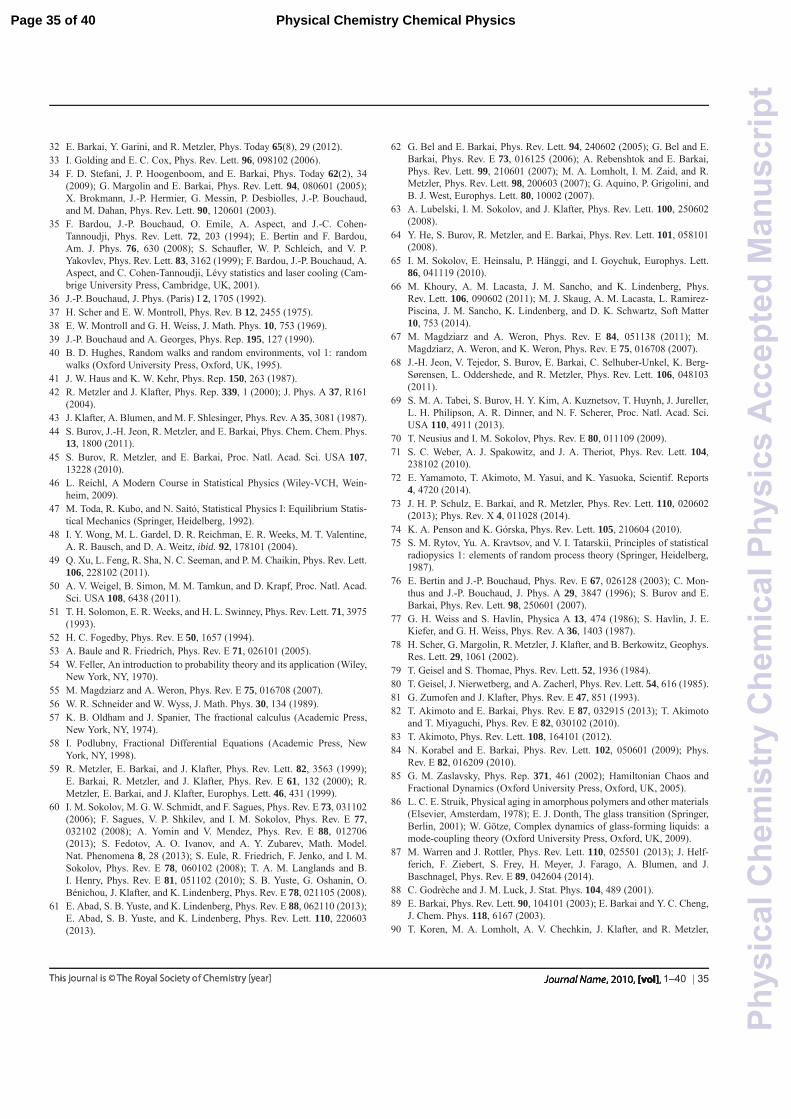
32 E. Barkai, Y. Garini, and R. Metzler, Phys. Today 65(8), 29 (2012).33 I. Golding and E. C. Cox, Phys. Rev. Lett. 96, 098102 (2006).34 F. D. Stefani, J. P. Hoogenboom, and E. Barkai, Phys. Today 62(2), 34

(2009); G. Margolin and E. Barkai, Phys. Rev. Lett. 94, 080601 (2005);X. Brokmann, J.-P. Hermier, G. Messin, P. Desbiolles, J.-P. Bouchaud,and M. Dahan, Phys. Rev. Lett. 90, 120601 (2003).

35 F. Bardou, J.-P. Bouchaud, O. Emile, A. Aspect, and J.-C. Cohen-Tannoudji, Phys. Rev. Lett. 72, 203 (1994); E. Bertin and F. Bardou,Am. J. Phys. 76, 630 (2008); S. Schaufler, W. P. Schleich, and V. P.Yakovlev, Phys. Rev. Lett. 83, 3162 (1999); F. Bardou, J.-P. Bouchaud, A.Aspect, and C. Cohen-Tannoudji, Levy statistics and laser cooling (Cam-brige University Press, Cambridge, UK, 2001).

36 J.-P. Bouchaud, J. Phys. (Paris) I 2, 1705 (1992).37 H. Scher and E. W. Montroll, Phys. Rev. B 12, 2455 (1975).38 E. W. Montroll and G. H. Weiss, J. Math. Phys. 10, 753 (1969).39 J.-P. Bouchaud and A. Georges, Phys. Rep. 195, 127 (1990).40 B. D. Hughes, Random walks and random environments, vol 1: random

walks (Oxford University Press, Oxford, UK, 1995).41 J. W. Haus and K. W. Kehr, Phys. Rep. 150, 263 (1987).42 R. Metzler and J. Klafter, Phys. Rep. 339, 1 (2000); J. Phys. A 37, R161

(2004).43 J. Klafter, A. Blumen, and M. F. Shlesinger, Phys. Rev. A 35, 3081 (1987).44 S. Burov, J.-H. Jeon, R. Metzler, and E. Barkai, Phys. Chem. Chem. Phys.

13, 1800 (2011).45 S. Burov, R. Metzler, and E. Barkai, Proc. Natl. Acad. Sci. USA 107,

13228 (2010).46 L. Reichl, A Modern Course in Statistical Physics (Wiley-VCH, Wein-

heim, 2009).47 M. Toda, R. Kubo, and N. Saito, Statistical Physics I: Equilibrium Statis-

tical Mechanics (Springer, Heidelberg, 1992).48 I. Y. Wong, M. L. Gardel, D. R. Reichman, E. R. Weeks, M. T. Valentine,

A. R. Bausch, and D. A. Weitz, ibid. 92, 178101 (2004).49 Q. Xu, L. Feng, R. Sha, N. C. Seeman, and P. M. Chaikin, Phys. Rev. Lett.

106, 228102 (2011).50 A. V. Weigel, B. Simon, M. M. Tamkun, and D. Krapf, Proc. Natl. Acad.

Sci. USA 108, 6438 (2011).51 T. H. Solomon, E. R. Weeks, and H. L. Swinney, Phys. Rev. Lett. 71, 3975

(1993).52 H. C. Fogedby, Phys. Rev. E 50, 1657 (1994).53 A. Baule and R. Friedrich, Phys. Rev. E 71, 026101 (2005).54 W. Feller, An introduction to probability theory and its application (Wiley,

New York, NY, 1970).55 M. Magdziarz and A. Weron, Phys. Rev. E 75, 016708 (2007).56 W. R. Schneider and W. Wyss, J. Math. Phys. 30, 134 (1989).57 K. B. Oldham and J. Spanier, The fractional calculus (Academic Press,

New York, NY, 1974).58 I. Podlubny, Fractional Differential Equations (Academic Press, New

York, NY, 1998).59 R. Metzler, E. Barkai, and J. Klafter, Phys. Rev. Lett. 82, 3563 (1999);

E. Barkai, R. Metzler, and J. Klafter, Phys. Rev. E 61, 132 (2000); R.Metzler, E. Barkai, and J. Klafter, Europhys. Lett. 46, 431 (1999).

60 I. M. Sokolov, M. G. W. Schmidt, and F. Sagues, Phys. Rev. E 73, 031102(2006); F. Sagues, V. P. Shkilev, and I. M. Sokolov, Phys. Rev. E 77,032102 (2008); A. Yomin and V. Mendez, Phys. Rev. E 88, 012706(2013); S. Fedotov, A. O. Ivanov, and A. Y. Zubarev, Math. Model.Nat. Phenomena 8, 28 (2013); S. Eule, R. Friedrich, F. Jenko, and I. M.Sokolov, Phys. Rev. E 78, 060102 (2008); T. A. M. Langlands and B.I. Henry, Phys. Rev. E 81, 051102 (2010); S. B. Yuste, G. Oshanin, O.Benichou, J. Klafter, and K. Lindenberg, Phys. Rev. E 78, 021105 (2008).

61 E. Abad, S. B. Yuste, and K. Lindenberg, Phys. Rev. E 88, 062110 (2013);E. Abad, S. B. Yuste, and K. Lindenberg, Phys. Rev. Lett. 110, 220603(2013).

62 G. Bel and E. Barkai, Phys. Rev. Lett. 94, 240602 (2005); G. Bel and E.Barkai, Phys. Rev. E 73, 016125 (2006); A. Rebenshtok and E. Barkai,Phys. Rev. Lett. 99, 210601 (2007); M. A. Lomholt, I. M. Zaid, and R.Metzler, Phys. Rev. Lett. 98, 200603 (2007); G. Aquino, P. Grigolini, andB. J. West, Europhys. Lett. 80, 10002 (2007).

63 A. Lubelski, I. M. Sokolov, and J. Klafter, Phys. Rev. Lett. 100, 250602(2008).

64 Y. He, S. Burov, R. Metzler, and E. Barkai, Phys. Rev. Lett. 101, 058101(2008).

65 I. M. Sokolov, E. Heinsalu, P. Hanggi, and I. Goychuk, Europhys. Lett.86, 041119 (2010).

66 M. Khoury, A. M. Lacasta, J. M. Sancho, and K. Lindenberg, Phys.Rev. Lett. 106, 090602 (2011); M. J. Skaug, A. M. Lacasta, L. Ramirez-Piscina, J. M. Sancho, K. Lindenberg, and D. K. Schwartz, Soft Matter10, 753 (2014).

67 M. Magdziarz and A. Weron, Phys. Rev. E 84, 051138 (2011); M.Magdziarz, A. Weron, and K. Weron, Phys. Rev. E 75, 016708 (2007).

68 J.-H. Jeon, V. Tejedor, S. Burov, E. Barkai, C. Selhuber-Unkel, K. Berg-Sørensen, L. Oddershede, and R. Metzler, Phys. Rev. Lett. 106, 048103(2011).

69 S. M. A. Tabei, S. Burov, H. Y. Kim, A. Kuznetsov, T. Huynh, J. Jureller,L. H. Philipson, A. R. Dinner, and N. F. Scherer, Proc. Natl. Acad. Sci.USA 110, 4911 (2013).

70 T. Neusius and I. M. Sokolov, Phys. Rev. E 80, 011109 (2009).71 S. C. Weber, A. J. Spakowitz, and J. A. Theriot, Phys. Rev. Lett. 104,

238102 (2010).72 E. Yamamoto, T. Akimoto, M. Yasui, and K. Yasuoka, Scientif. Reports

4, 4720 (2014).73 J. H. P. Schulz, E. Barkai, and R. Metzler, Phys. Rev. Lett. 110, 020602

(2013); Phys. Rev. X 4, 011028 (2014).74 K. A. Penson and K. Gorska, Phys. Rev. Lett. 105, 210604 (2010).75 S. M. Rytov, Yu. A. Kravtsov, and V. I. Tatarskii, Principles of statistical

radiopysics 1: elements of random process theory (Springer, Heidelberg,1987).

76 E. Bertin and J.-P. Bouchaud, Phys. Rev. E 67, 026128 (2003); C. Mon-thus and J.-P. Bouchaud, J. Phys. A 29, 3847 (1996); S. Burov and E.Barkai, Phys. Rev. Lett. 98, 250601 (2007).

77 G. H. Weiss and S. Havlin, Physica A 13, 474 (1986); S. Havlin, J. E.Kiefer, and G. H. Weiss, Phys. Rev. A 36, 1403 (1987).

78 H. Scher, G. Margolin, R. Metzler, J. Klafter, and B. Berkowitz, Geophys.Res. Lett. 29, 1061 (2002).

79 T. Geisel and S. Thomae, Phys. Rev. Lett. 52, 1936 (1984).80 T. Geisel, J. Nierwetberg, and A. Zacherl, Phys. Rev. Lett. 54, 616 (1985).81 G. Zumofen and J. Klafter, Phys. Rev. E 47, 851 (1993).82 T. Akimoto and E. Barkai, Phys. Rev. E 87, 032915 (2013); T. Akimoto

and T. Miyaguchi, Phys. Rev. E 82, 030102 (2010).83 T. Akimoto, Phys. Rev. Lett. 108, 164101 (2012).84 N. Korabel and E. Barkai, Phys. Rev. Lett. 102, 050601 (2009); Phys.

Rev. E 82, 016209 (2010).85 G. M. Zaslavsky, Phys. Rep. 371, 461 (2002); Hamiltonian Chaos and

Fractional Dynamics (Oxford University Press, Oxford, UK, 2005).86 L. C. E. Struik, Physical aging in amorphous polymers and other materials

(Elsevier, Amsterdam, 1978); E. J. Donth, The glass transition (Springer,Berlin, 2001); W. Gotze, Complex dynamics of glass-forming liquids: amode-coupling theory (Oxford University Press, Oxford, UK, 2009).

87 M. Warren and J. Rottler, Phys. Rev. Lett. 110, 025501 (2013); J. Helf-ferich, F. Ziebert, S. Frey, H. Meyer, J. Farago, A. Blumen, and J.Baschnagel, Phys. Rev. E 89, 042604 (2014).

88 C. Godreche and J. M. Luck, J. Stat. Phys. 104, 489 (2001).89 E. Barkai, Phys. Rev. Lett. 90, 104101 (2003); E. Barkai and Y. C. Cheng,

J. Chem. Phys. 118, 6167 (2003).90 T. Koren, M. A. Lomholt, A. V. Chechkin, J. Klafter, and R. Metzler,

1–40 | 35

Page 35 of 40 Physical Chemistry Chemical Physics

Phy

sica

lChe

mis

try

Che

mic

alP

hysi

csA

ccep

ted

Man

uscr

ipt

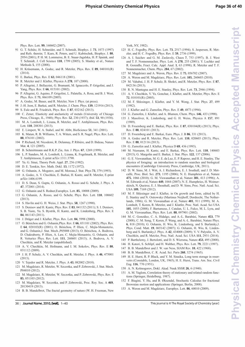
Phys. Rev. Lett. 99, 160602 (2007).91 G. T. Schutz, H. Schneider, and T. Schmidt, Biophys. J. 73, 1073 (1997)

and Refs. therein; T. Kues, R. Peters, and U. Kubitschek, Biophys. J. 80,2954 (2001); P. H. M. Lommerse, B. E. Snaar-Jagalska, H. P. Spaink, andT. Schmidt, J. Cell Science 118, 1799 (2005); S. Manley et al., NatureMethods 5, 155 (2008).

92 H. Krusemann, A. Godec, and R. Metzler, Phys. Rev. E 89, 040101(R)(2014).

93 E. Barkai, Phys. Rev. E 63, 046118 (2001).94 R. Metzler and J. Klafter, Physica A 278, 107 (2000).95 P. Allegrini, J. Bellazzini, G. Bramanti, M. Ignaccolo, P. Grigolini, and J.

Yang, Phys. Rev. E 66, 015101 (2002).96 P. Allegrini, G. Aquino, P. Grigolini, L. Palatella, A. Rosa, and B. J. West,

Phys. Rev. E 71, 066109 (2005).97 A. Godec, M. Bauer, and R. Metzler, New J. Phys. (at press).98 J.-H. Jeon, E. Barkai, and R. Metzler, J. Chem. Phys. 139, 121916 (2013).99 S. Eule and R. Friedrich, Phys. Rev. E 87, 032162 (2013).100 C. Zener, Elasticity and anelasticity of metals (University of Chicago

Press, Chicago, IL, 1948); Phys. Rev. 52, 230 (1937); ibid. 53, 90 (1938).101 M. A. Lomholt, L. Lizana, R. Metzler, and T. Ambjornsson, Phys. Rev.

Lett. 110, 208301 (2013).102 E. Limpert, W. A. Stahel, and M. Abbt, BioScience 51, 341 (2001).103 K. Matan, R. B. Williams, T. A. Witten, and S. R. Nagel, Phys. Rev. Lett.

88, 076101 (2002).104 P. Richard, M. Nicodemi, R. Delannay, P. Ribiere, and D. Bideau, Nature

Mat. 4, 121 (2005).105 B. Schmittmann and R.K.P. Zia, Am. J. Phys. 67, 1269 (1999).106 L. P. Sanders, M. A. Lomholt, L. Lizana, K. Fogelmark, R. Metzler, and

T. Ambjornsson, E-print arXiv:1311.3790.107 Ya. G. Sinai, Theory Prob. Appl. 27, 256 (1982).108 D. E. Temkin, Sov. Math. Dokl. 13, 1172 (1972).109 G. Oshanin, A. Mogutov, and M. Moreau,J. Stat. Phys 73, 379 (1993).110 A. Godec, A. V. Chechkin, E. Barkai, H. Kantz, and R. Metzler, E-print

arXiv:1406.6199.111 D. S. Dean, S. Gupta, G. Oshanin, A. Rosso and G. Schehr, J. Phys. A

47, 372001 (2014).112 G. Oshanin and S. Redner,Europhys. Lett. 85, 10008 (2009).113 G. Oshanin, A. Rosso, and G. Schehr, Phys. Rev. Lett. 110, 100602

(2013).114 S. Havlin and G. H. Weiss, J. Stat. Phys. 58, 1267 (1990).115 S. Denisov and H. Kantz, Phys. Rev. E 83, 041132 (2011); S. I. Denisov,

S. B. Yuste, Yu. S. Bystrik, H. Kantz, and K. Lindenberg, Phys. Rev. E84, 061143 (2011).

116 J. Drager and J. Klafter, Phys. Rev. Lett. 84, 5998 (2000).117 O. Benichou and G. Oshanin,Phys. Rev. E 66, 031101 (2002); Phys. Rev.

E 64, 020103(R) (2001); O. Benichou, P. Illien, C. Mejıa-Monasterio,and G. Oshanin,J. Stat. Mech.,P05008 (2013); O. Benichou, A. Bodrova,D. Chakraborty, P. Illien, A. Law, C. Mejıa-Monastrio, G. Oshanin, andR. Voituriez Phys. Rev. Lett. 111, 260601 (2013); A. Bodrova, A. V.Chechkin, and R. Metzler (unpublished).

118 A. V. Chechkin, M. Hofmann, and I. M. Sokolov, Phys. Rev. E 80,031112 (2009).

119 J. H. P. Schulz, A. V. Chechkin, and R. Metzler, J. Phys. A 46, 475001(2013).

120 V. Tejedor and R. Metzler, J. Phys. A 43, 082002 (2010).121 M. Magdziarz, R. Metzler, W. Szczotka, and P. Zebrowski, J. Stat. Mech.

P04010 (2012).122 M. Magdziarz, R. Metzler, W. Szczotka, and P. Zebrowski, Phys. Rev. E

85, 051103 (2012).123 M. Magdziarz, W. Szczotka, and P. Zebrowski, Proc. Roy. Soc. A 469,

20130419 (2013).124 B. B. Mandelbrot, The fractal geometry of nature (W. H. Freeman, New

York, NY, 1982).125 H. C. Fogedby, Phys. Rev. Lett. 73, 2517 (1994); S. Jespersen, R. Met-

zler, and H. C. Fogedby, Phys. Rev. E 59, 2736 (1999).126 A. I. Saichev and G. M. Zaslavsly, Chaos 7, 753 (1997); B. J. West

and T. F. Nonnenmacher, Phys. Lett. A 278, 255 (2001); Y. Luchko andR. Gorenflo, Fract. Calc. Appl. Anal. 1, 63 (1998); R. Metzler and T. F.Nonnenmacher, Chem. Phys. 284, 67 (2002).

127 M. Magdziarz and A. Weron, Phys. Rev. E 75, 056702 (2007).128 A. Weron and M. Magdziarz, Phys. Rev. Lett. 105, 260603 (2010).129 M. Vahabai, J. H. P. Schulz, B. Shokri, and R. Metzler, Phys. Rev. E 87,

042136 (2013).130 R. N. Mantegna and H. E. Stanley, Phys. Rev. Lett. 73, 2946 (1994).131 A. V. Chechkin, V. Yu. Gonchar, J. Klafter, and R. Metzler, Phys. Rev. E

72, 010101(R) (2005).132 M. F. Shlesinger, J. Klafter, and Y. M. Wong, J. Stat. Phys. 27, 499

(1982).133 J. Klafter and G. Zumofen, Phys. Rev. E 49, 4873 (1994).134 G. Zumofen, J. Klafter, and A. Blumen, Chem. Phys. 146, 433 (1990).135 J. Masoliver, K. Lindenberg, and G. H. Weiss, Physica A 157, 891

(1989).136 D. Froemberg and E. Barkai, Phys. Rev. E 87, 030104(R) (2013); Phys.

Rev. E 88, 024101 (2013).137 D. Froemberg and E. Barkai, Euro. Phys. J. B 86, 331 (2013).138 A. Godec and R. Metzler, Phys. Rev. Lett. 110, 020603 (2013); Phys.

Rev. E 88, 012116 (2013).139 G. Zumofen and J. Klafter, Physica D 69, 436 (1993).140 M. Niemann, H. Kantz, and E. Barkai, Phys. Rev. Lett. 110, 140603

(2013); G. Margolin and E. Barkai, J. Stat. Phys. 122, 137 (2006).141 G. E. Viswanathan, M. G. E. da Luz, E. P. Raposo, and H. E. Stanley, The

physica of foraging: an introduction to random searches and biologicalencounters (Cambridge University Press, Cambridge, UK, 2011).

142 D. W. Sims, M. J. Witt, A. J. Richardson, E. J. Southall, and J. D. Met-calfe, Proc. Biol. Sci. 273, 1195 (2006); N. E. Humphries et al, Nature475, 1066 (2010); G. M. Viswanathan et al, Nature 381, 413 (1996); A.M. Edwards et al, Nature 449, 1044 (2007); N. E. Humphries, H. Weimer-skirch, N. Queiroz, E. J. Shouthall, and D. W. Sims, Proc. Natl. Acad. Sci.USA 109, 7169 (2012).

143 M. F. Shlesinger and J. Klafter, in On growth and form, edited by H.E. Stanley and N. Ostrowsky (Martinus Neijhoff, Dordrecht, The Nether-lands, 1986); G. M. Viswanathan et al, Nature 401, 911 (1999); M. A.Lomholt, T. Koren, R. Metzler, and J. Klatfer, Proc. Natl. Acad. Sci USA105, 1055 (2008); F. Bartumeus, J. Catalan, U. L. Fulco, M. L. Lyra, andG. M. Viswanathan, Phys. Rev. Lett. 88, 097901 (2002).

144 M. C. Gonzalez, C. A. Hidalgo, and A.-L. Barabasi, Nature 453, 779(2008); C. M. Song, T. Koren, P. Wang, and A.-L. Barabasi, Nature Phys.6, 818 (2010); G. Oshanin, H. Wio, K. Lindenberg, and S. Burlatsky,J.Phys. Cond. Matt. 19, 065142 (2007); G. Oshanin, H. Wio, K. Linden-berg and S. Burlatsky,J. Phys. A 42, 434008 (2009); V. V. Palyulin, A. V.Chechkin, and R. Metzler, Proc. Natl. Acad. Sci. USA 111, 2931 (2014).

145 P. Barthelemy, J. Bertolotti, and D. S. Wiersma, Nature 453, 495 (2008).146 H. Katori, S. Schlipf, and H. Walther, Phys. Rev. Lett. 79, 2221 (1997).147 B. B. Mandelbrot and J. W. van Ness, SIAM Rev. 10, 422 (1968).148 B. B. Mandelbrot, C. R. Acad. Sci. Paris 260, 3274 (1965).149 H. E. Hurst, R. P. Black, and Y. M. Sinaika, Long term storage in reser-

voirs (Constable, London, UK, 1965); H. E. Hurst, Trans. Am. Soc. CivilEng. 116, 770 (1951).

150 A. N. Kolmogorov, Dokl. Akad. Nauk SSSR 26, 6 (1940).151 A. M. Yaglom, Correlation theory of stationary and related random func-

tions (Springer, Heidelberg, 1987).152 F. Biagini, Y. Hu, and B. Øksendal, Stochastic Calculus for fractional

Brownian motion and applications (Springer, Berlin, 2008).153 A. Weron and M. Magdziarz, Europhys. Lett. 86, 60010 (2009).

36 | 1–40

Page 36 of 40Physical Chemistry Chemical Physics

Phy

sica

lChe

mis

try

Che

mic

alP

hysi

csA

ccep

ted

Man

uscr

ipt

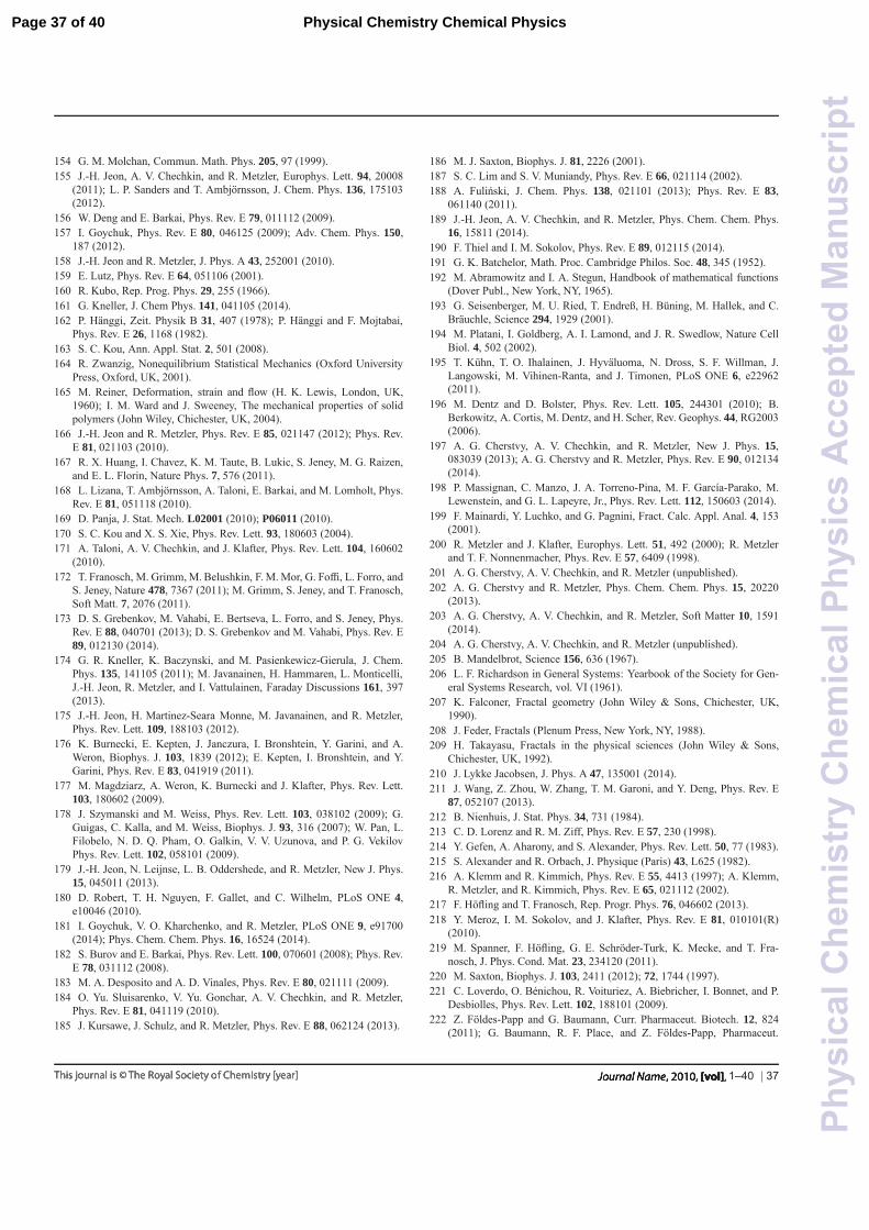
154 G. M. Molchan, Commun. Math. Phys. 205, 97 (1999).155 J.-H. Jeon, A. V. Chechkin, and R. Metzler, Europhys. Lett. 94, 20008

(2011); L. P. Sanders and T. Ambjornsson, J. Chem. Phys. 136, 175103(2012).

156 W. Deng and E. Barkai, Phys. Rev. E 79, 011112 (2009).157 I. Goychuk, Phys. Rev. E 80, 046125 (2009); Adv. Chem. Phys. 150,

187 (2012).158 J.-H. Jeon and R. Metzler, J. Phys. A 43, 252001 (2010).159 E. Lutz, Phys. Rev. E 64, 051106 (2001).160 R. Kubo, Rep. Prog. Phys. 29, 255 (1966).161 G. Kneller, J. Chem Phys. 141, 041105 (2014).162 P. Hanggi, Zeit. Physik B 31, 407 (1978); P. Hanggi and F. Mojtabai,

Phys. Rev. E 26, 1168 (1982).163 S. C. Kou, Ann. Appl. Stat. 2, 501 (2008).164 R. Zwanzig, Nonequilibrium Statistical Mechanics (Oxford University

Press, Oxford, UK, 2001).165 M. Reiner, Deformation, strain and flow (H. K. Lewis, London, UK,

1960); I. M. Ward and J. Sweeney, The mechanical properties of solidpolymers (John Wiley, Chichester, UK, 2004).

166 J.-H. Jeon and R. Metzler, Phys. Rev. E 85, 021147 (2012); Phys. Rev.E 81, 021103 (2010).

167 R. X. Huang, I. Chavez, K. M. Taute, B. Lukic, S. Jeney, M. G. Raizen,and E. L. Florin, Nature Phys. 7, 576 (2011).

168 L. Lizana, T. Ambjornsson, A. Taloni, E. Barkai, and M. Lomholt, Phys.Rev. E 81, 051118 (2010).

169 D. Panja, J. Stat. Mech. L02001 (2010); P06011 (2010).170 S. C. Kou and X. S. Xie, Phys. Rev. Lett. 93, 180603 (2004).171 A. Taloni, A. V. Chechkin, and J. Klafter, Phys. Rev. Lett. 104, 160602

(2010).172 T. Franosch, M. Grimm, M. Belushkin, F. M. Mor, G. Foffi, L. Forro, and

S. Jeney, Nature 478, 7367 (2011); M. Grimm, S. Jeney, and T. Franosch,Soft Matt. 7, 2076 (2011).

173 D. S. Grebenkov, M. Vahabi, E. Bertseva, L. Forro, and S. Jeney, Phys.Rev. E 88, 040701 (2013); D. S. Grebenkov and M. Vahabi, Phys. Rev. E89, 012130 (2014).

174 G. R. Kneller, K. Baczynski, and M. Pasienkewicz-Gierula, J. Chem.Phys. 135, 141105 (2011); M. Javanainen, H. Hammaren, L. Monticelli,J.-H. Jeon, R. Metzler, and I. Vattulainen, Faraday Discussions 161, 397(2013).

175 J.-H. Jeon, H. Martinez-Seara Monne, M. Javanainen, and R. Metzler,Phys. Rev. Lett. 109, 188103 (2012).

176 K. Burnecki, E. Kepten, J. Janczura, I. Bronshtein, Y. Garini, and A.Weron, Biophys. J. 103, 1839 (2012); E. Kepten, I. Bronshtein, and Y.Garini, Phys. Rev. E 83, 041919 (2011).

177 M. Magdziarz, A. Weron, K. Burnecki and J. Klafter, Phys. Rev. Lett.103, 180602 (2009).

178 J. Szymanski and M. Weiss, Phys. Rev. Lett. 103, 038102 (2009); G.Guigas, C. Kalla, and M. Weiss, Biophys. J. 93, 316 (2007); W. Pan, L.Filobelo, N. D. Q. Pham, O. Galkin, V. V. Uzunova, and P. G. VekilovPhys. Rev. Lett. 102, 058101 (2009).

179 J.-H. Jeon, N. Leijnse, L. B. Oddershede, and R. Metzler, New J. Phys.15, 045011 (2013).

180 D. Robert, T. H. Nguyen, F. Gallet, and C. Wilhelm, PLoS ONE 4,e10046 (2010).

181 I. Goychuk, V. O. Kharchenko, and R. Metzler, PLoS ONE 9, e91700(2014); Phys. Chem. Chem. Phys. 16, 16524 (2014).

182 S. Burov and E. Barkai, Phys. Rev. Lett. 100, 070601 (2008); Phys. Rev.E 78, 031112 (2008).

183 M. A. Desposito and A. D. Vinales, Phys. Rev. E 80, 021111 (2009).184 O. Yu. Sluisarenko, V. Yu. Gonchar, A. V. Chechkin, and R. Metzler,

Phys. Rev. E 81, 041119 (2010).185 J. Kursawe, J. Schulz, and R. Metzler, Phys. Rev. E 88, 062124 (2013).

186 M. J. Saxton, Biophys. J. 81, 2226 (2001).187 S. C. Lim and S. V. Muniandy, Phys. Rev. E 66, 021114 (2002).188 A. Fulinski, J. Chem. Phys. 138, 021101 (2013); Phys. Rev. E 83,

061140 (2011).189 J.-H. Jeon, A. V. Chechkin, and R. Metzler, Phys. Chem. Chem. Phys.

16, 15811 (2014).190 F. Thiel and I. M. Sokolov, Phys. Rev. E 89, 012115 (2014).191 G. K. Batchelor, Math. Proc. Cambridge Philos. Soc. 48, 345 (1952).192 M. Abramowitz and I. A. Stegun, Handbook of mathematical functions

(Dover Publ., New York, NY, 1965).193 G. Seisenberger, M. U. Ried, T. Endreß, H. Buning, M. Hallek, and C.

Brauchle, Science 294, 1929 (2001).194 M. Platani, I. Goldberg, A. I. Lamond, and J. R. Swedlow, Nature Cell

Biol. 4, 502 (2002).195 T. Kuhn, T. O. Ihalainen, J. Hyvaluoma, N. Dross, S. F. Willman, J.

Langowski, M. Vihinen-Ranta, and J. Timonen, PLoS ONE 6, e22962(2011).

196 M. Dentz and D. Bolster, Phys. Rev. Lett. 105, 244301 (2010); B.Berkowitz, A. Cortis, M. Dentz, and H. Scher, Rev. Geophys. 44, RG2003(2006).

197 A. G. Cherstvy, A. V. Chechkin, and R. Metzler, New J. Phys. 15,083039 (2013); A. G. Cherstvy and R. Metzler, Phys. Rev. E 90, 012134(2014).

198 P. Massignan, C. Manzo, J. A. Torreno-Pina, M. F. Garcıa-Parako, M.Lewenstein, and G. L. Lapeyre, Jr., Phys. Rev. Lett. 112, 150603 (2014).

199 F. Mainardi, Y. Luchko, and G. Pagnini, Fract. Calc. Appl. Anal. 4, 153(2001).

200 R. Metzler and J. Klafter, Europhys. Lett. 51, 492 (2000); R. Metzlerand T. F. Nonnenmacher, Phys. Rev. E 57, 6409 (1998).

201 A. G. Cherstvy, A. V. Chechkin, and R. Metzler (unpublished).202 A. G. Cherstvy and R. Metzler, Phys. Chem. Chem. Phys. 15, 20220

(2013).203 A. G. Cherstvy, A. V. Chechkin, and R. Metzler, Soft Matter 10, 1591

(2014).204 A. G. Cherstvy, A. V. Chechkin, and R. Metzler (unpublished).205 B. Mandelbrot, Science 156, 636 (1967).206 L. F. Richardson in General Systems: Yearbook of the Society for Gen-

eral Systems Research, vol. VI (1961).207 K. Falconer, Fractal geometry (John Wiley & Sons, Chichester, UK,

1990).208 J. Feder, Fractals (Plenum Press, New York, NY, 1988).209 H. Takayasu, Fractals in the physical sciences (John Wiley & Sons,

Chichester, UK, 1992).210 J. Lykke Jacobsen, J. Phys. A 47, 135001 (2014).211 J. Wang, Z. Zhou, W. Zhang, T. M. Garoni, and Y. Deng, Phys. Rev. E

87, 052107 (2013).212 B. Nienhuis, J. Stat. Phys. 34, 731 (1984).213 C. D. Lorenz and R. M. Ziff, Phys. Rev. E 57, 230 (1998).214 Y. Gefen, A. Aharony, and S. Alexander, Phys. Rev. Lett. 50, 77 (1983).215 S. Alexander and R. Orbach, J. Physique (Paris) 43, L625 (1982).216 A. Klemm and R. Kimmich, Phys. Rev. E 55, 4413 (1997); A. Klemm,

R. Metzler, and R. Kimmich, Phys. Rev. E 65, 021112 (2002).217 F. Hofling and T. Franosch, Rep. Progr. Phys. 76, 046602 (2013).218 Y. Meroz, I. M. Sokolov, and J. Klafter, Phys. Rev. E 81, 010101(R)

(2010).219 M. Spanner, F. Hofling, G. E. Schroder-Turk, K. Mecke, and T. Fra-

nosch, J. Phys. Cond. Mat. 23, 234120 (2011).220 M. Saxton, Biophys. J. 103, 2411 (2012); 72, 1744 (1997).221 C. Loverdo, O. Benichou, R. Voituriez, A. Biebricher, I. Bonnet, and P.

Desbiolles, Phys. Rev. Lett. 102, 188101 (2009).222 Z. Foldes-Papp and G. Baumann, Curr. Pharmaceut. Biotech. 12, 824

(2011); G. Baumann, R. F. Place, and Z. Foldes-Papp, Pharmaceut.

1–40 | 37

Page 37 of 40 Physical Chemistry Chemical Physics

Phy

sica

lChe

mis

try

Che

mic

alP

hysi

csA

ccep

ted

Man

uscr

ipt

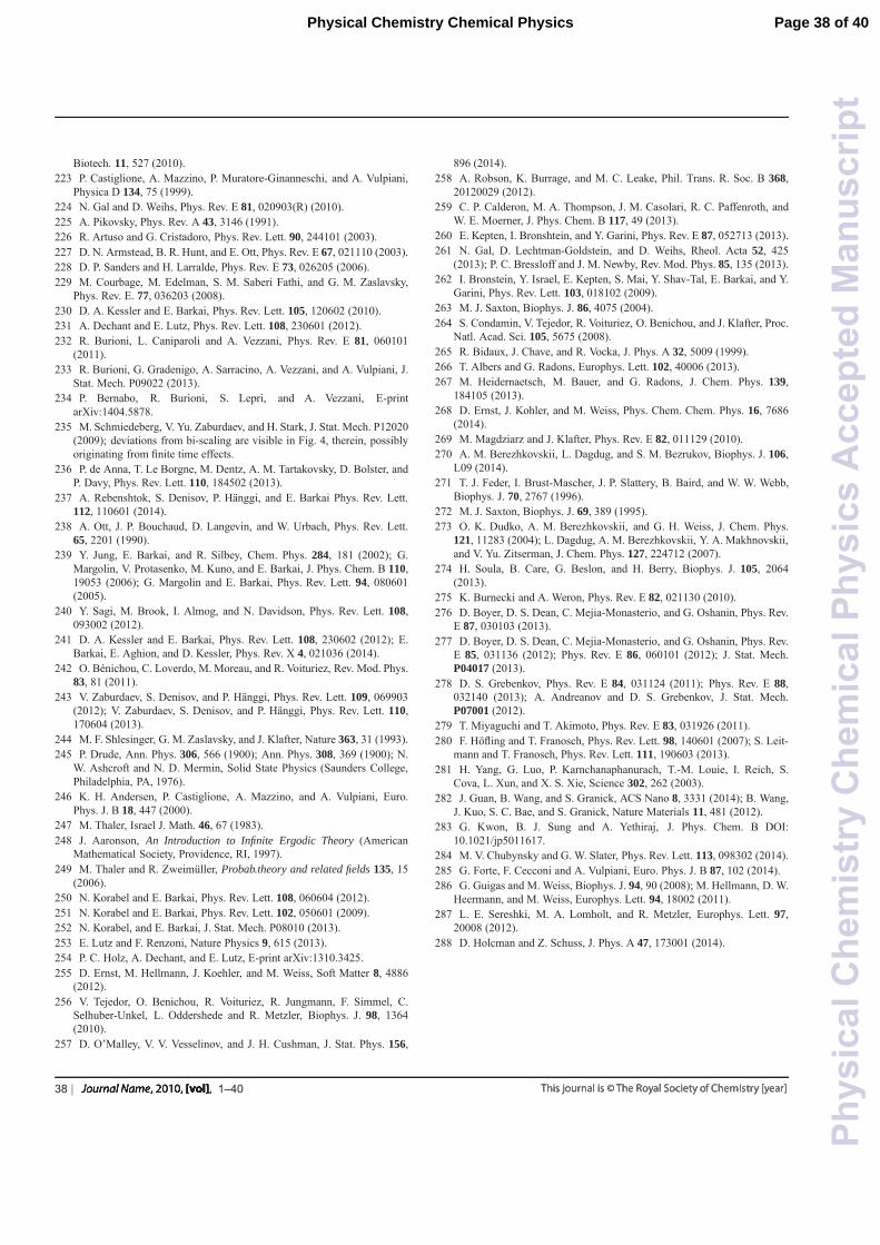
Biotech. 11, 527 (2010).223 P. Castiglione, A. Mazzino, P. Muratore-Ginanneschi, and A. Vulpiani,

Physica D 134, 75 (1999).224 N. Gal and D. Weihs, Phys. Rev. E 81, 020903(R) (2010).225 A. Pikovsky, Phys. Rev. A 43, 3146 (1991).226 R. Artuso and G. Cristadoro, Phys. Rev. Lett. 90, 244101 (2003).227 D. N. Armstead, B. R. Hunt, and E. Ott, Phys. Rev. E 67, 021110 (2003).228 D. P. Sanders and H. Larralde, Phys. Rev. E 73, 026205 (2006).229 M. Courbage, M. Edelman, S. M. Saberi Fathi, and G. M. Zaslavsky,

Phys. Rev. E. 77, 036203 (2008).230 D. A. Kessler and E. Barkai, Phys. Rev. Lett. 105, 120602 (2010).231 A. Dechant and E. Lutz, Phys. Rev. Lett. 108, 230601 (2012).232 R. Burioni, L. Caniparoli and A. Vezzani, Phys. Rev. E 81, 060101

(2011).233 R. Burioni, G. Gradenigo, A. Sarracino, A. Vezzani, and A. Vulpiani, J.

Stat. Mech. P09022 (2013).234 P. Bernabo, R. Burioni, S. Lepri, and A. Vezzani, E-print

arXiv:1404.5878.235 M. Schmiedeberg, V. Yu. Zaburdaev, and H. Stark, J. Stat. Mech. P12020

(2009); deviations from bi-scaling are visible in Fig. 4, therein, possiblyoriginating from finite time effects.

236 P. de Anna, T. Le Borgne, M. Dentz, A. M. Tartakovsky, D. Bolster, andP. Davy, Phys. Rev. Lett. 110, 184502 (2013).

237 A. Rebenshtok, S. Denisov, P. Hanggi, and E. Barkai Phys. Rev. Lett.112, 110601 (2014).

238 A. Ott, J. P. Bouchaud, D. Langevin, and W. Urbach, Phys. Rev. Lett.65, 2201 (1990).

239 Y. Jung, E. Barkai, and R. Silbey, Chem. Phys. 284, 181 (2002); G.Margolin, V. Protasenko, M. Kuno, and E. Barkai, J. Phys. Chem. B 110,19053 (2006); G. Margolin and E. Barkai, Phys. Rev. Lett. 94, 080601(2005).

240 Y. Sagi, M. Brook, I. Almog, and N. Davidson, Phys. Rev. Lett. 108,093002 (2012).

241 D. A. Kessler and E. Barkai, Phys. Rev. Lett. 108, 230602 (2012); E.Barkai, E. Aghion, and D. Kessler, Phys. Rev. X 4, 021036 (2014).

242 O. Benichou, C. Loverdo, M. Moreau, and R. Voituriez, Rev. Mod. Phys.83, 81 (2011).

243 V. Zaburdaev, S. Denisov, and P. Hanggi, Phys. Rev. Lett. 109, 069903(2012); V. Zaburdaev, S. Denisov, and P. Hanggi, Phys. Rev. Lett. 110,170604 (2013).

244 M. F. Shlesinger, G. M. Zaslavsky, and J. Klafter, Nature 363, 31 (1993).245 P. Drude, Ann. Phys. 306, 566 (1900); Ann. Phys. 308, 369 (1900); N.

W. Ashcroft and N. D. Mermin, Solid State Physics (Saunders College,Philadelphia, PA, 1976).

246 K. H. Andersen, P. Castiglione, A. Mazzino, and A. Vulpiani, Euro.Phys. J. B 18, 447 (2000).

247 M. Thaler, Israel J. Math. 46, 67 (1983).248 J. Aaronson, An Introduction to Infinite Ergodic Theory (American

Mathematical Society, Providence, RI, 1997).249 M. Thaler and R. Zweimuller, Probab.theory and related fields 135, 15

(2006).250 N. Korabel and E. Barkai, Phys. Rev. Lett. 108, 060604 (2012).251 N. Korabel and E. Barkai, Phys. Rev. Lett. 102, 050601 (2009).252 N. Korabel, and E. Barkai, J. Stat. Mech. P08010 (2013).253 E. Lutz and F. Renzoni, Nature Physics 9, 615 (2013).254 P. C. Holz, A. Dechant, and E. Lutz, E-print arXiv:1310.3425.255 D. Ernst, M. Hellmann, J. Koehler, and M. Weiss, Soft Matter 8, 4886

(2012).256 V. Tejedor, O. Benichou, R. Voituriez, R. Jungmann, F. Simmel, C.

Selhuber-Unkel, L. Oddershede and R. Metzler, Biophys. J. 98, 1364(2010).

257 D. O’Malley, V. V. Vesselinov, and J. H. Cushman, J. Stat. Phys. 156,

896 (2014).258 A. Robson, K. Burrage, and M. C. Leake, Phil. Trans. R. Soc. B 368,

20120029 (2012).259 C. P. Calderon, M. A. Thompson, J. M. Casolari, R. C. Paffenroth, and

W. E. Moerner, J. Phys. Chem. B 117, 49 (2013).260 E. Kepten, I. Bronshtein, and Y. Garini, Phys. Rev. E 87, 052713 (2013).261 N. Gal, D. Lechtman-Goldstein, and D. Weihs, Rheol. Acta 52, 425

(2013); P. C. Bressloff and J. M. Newby, Rev. Mod. Phys. 85, 135 (2013).262 I. Bronstein, Y. Israel, E. Kepten, S. Mai, Y. Shav-Tal, E. Barkai, and Y.

Garini, Phys. Rev. Lett. 103, 018102 (2009).263 M. J. Saxton, Biophys. J. 86, 4075 (2004).264 S. Condamin, V. Tejedor, R. Voituriez, O. Benichou, and J. Klafter, Proc.

Natl. Acad. Sci. 105, 5675 (2008).265 R. Bidaux, J. Chave, and R. Vocka, J. Phys. A 32, 5009 (1999).266 T. Albers and G. Radons, Europhys. Lett. 102, 40006 (2013).267 M. Heidernaetsch, M. Bauer, and G. Radons, J. Chem. Phys. 139,

184105 (2013).268 D. Ernst, J. Kohler, and M. Weiss, Phys. Chem. Chem. Phys. 16, 7686

(2014).269 M. Magdziarz and J. Klafter, Phys. Rev. E 82, 011129 (2010).270 A. M. Berezhkovskii, L. Dagdug, and S. M. Bezrukov, Biophys. J. 106,

L09 (2014).271 T. J. Feder, I. Brust-Mascher, J. P. Slattery, B. Baird, and W. W. Webb,

Biophys. J. 70, 2767 (1996).272 M. J. Saxton, Biophys. J. 69, 389 (1995).273 O. K. Dudko, A. M. Berezhkovskii, and G. H. Weiss, J. Chem. Phys.

121, 11283 (2004); L. Dagdug, A. M. Berezhkovskii, Y. A. Makhnovskii,and V. Yu. Zitserman, J. Chem. Phys. 127, 224712 (2007).

274 H. Soula, B. Care, G. Beslon, and H. Berry, Biophys. J. 105, 2064(2013).

275 K. Burnecki and A. Weron, Phys. Rev. E 82, 021130 (2010).276 D. Boyer, D. S. Dean, C. Mejia-Monasterio, and G. Oshanin, Phys. Rev.

E 87, 030103 (2013).277 D. Boyer, D. S. Dean, C. Mejia-Monasterio, and G. Oshanin, Phys. Rev.

E 85, 031136 (2012); Phys. Rev. E 86, 060101 (2012); J. Stat. Mech.P04017 (2013).

278 D. S. Grebenkov, Phys. Rev. E 84, 031124 (2011); Phys. Rev. E 88,032140 (2013); A. Andreanov and D. S. Grebenkov, J. Stat. Mech.P07001 (2012).

279 T. Miyaguchi and T. Akimoto, Phys. Rev. E 83, 031926 (2011).280 F. Hofling and T. Franosch, Phys. Rev. Lett. 98, 140601 (2007); S. Leit-

mann and T. Franosch, Phys. Rev. Lett. 111, 190603 (2013).281 H. Yang, G. Luo, P. Karnchanaphanurach, T.-M. Louie, I. Reich, S.

Cova, L. Xun, and X. S. Xie, Science 302, 262 (2003).282 J. Guan, B. Wang, and S. Granick, ACS Nano 8, 3331 (2014); B. Wang,

J. Kuo, S. C. Bae, and S. Granick, Nature Materials 11, 481 (2012).283 G. Kwon, B. J. Sung and A. Yethiraj, J. Phys. Chem. B DOI:

10.1021/jp5011617.284 M. V. Chubynsky and G. W. Slater, Phys. Rev. Lett. 113, 098302 (2014).285 G. Forte, F. Cecconi and A. Vulpiani, Euro. Phys. J. B 87, 102 (2014).286 G. Guigas and M. Weiss, Biophys. J. 94, 90 (2008); M. Hellmann, D. W.

Heermann, and M. Weiss, Europhys. Lett. 94, 18002 (2011).287 L. E. Sereshki, M. A. Lomholt, and R. Metzler, Europhys. Lett. 97,

20008 (2012).288 D. Holcman and Z. Schuss, J. Phys. A 47, 173001 (2014).

38 | 1–40

Page 38 of 40Physical Chemistry Chemical Physics

Phy

sica

lChe

mis

try

Che

mic

alP

hysi

csA

ccep

ted

Man

uscr

ipt

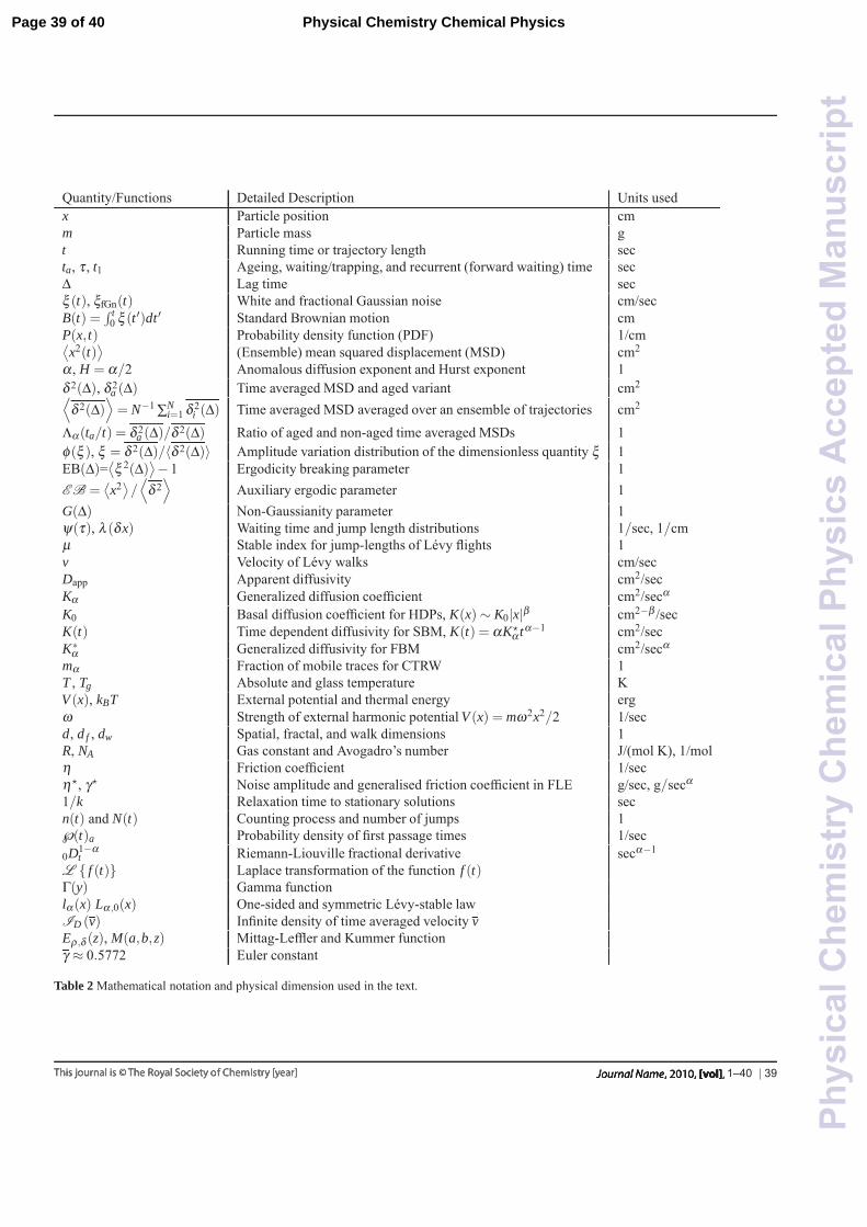
Quantity/Functions Detailed Description Units usedx Particle position cmm Particle mass gt Running time or trajectory length secta, τ , t1 Ageing, waiting/trapping, and recurrent (forward waiting) time secΔ Lag time secξ (t), ξfGn(t) White and fractional Gaussian noise cm/secB(t) =

∫ t0 ξ (t ′)dt ′ Standard Brownian motion cm

P(x, t) Probability density function (PDF) 1/cm⟨x2(t)

⟩(Ensemble) mean squared displacement (MSD) cm2

α , H = α/2 Anomalous diffusion exponent and Hurst exponent 1δ 2(Δ), δ 2

a (Δ) Time averaged MSD and aged variant cm2⟨δ 2(Δ)

⟩= N−1 ∑N

i=1 δ 2i (Δ) Time averaged MSD averaged over an ensemble of trajectories cm2

Λα(ta/t) = δ 2a (Δ)/δ 2(Δ) Ratio of aged and non-aged time averaged MSDs 1

φ(ξ ), ξ = δ 2(Δ)/〈δ 2(Δ)〉 Amplitude variation distribution of the dimensionless quantity ξ 1EB(Δ)=

⟨ξ 2(Δ)

⟩− 1 Ergodicity breaking parameter 1E B =

⟨x2⟩/⟨δ 2

⟩Auxiliary ergodic parameter 1

G(Δ) Non-Gaussianity parameter 1ψ(τ), λ (δx) Waiting time and jump length distributions 1/sec, 1/cmμ Stable index for jump-lengths of Levy flights 1v Velocity of Levy walks cm/secDapp Apparent diffusivity cm2/secKα Generalized diffusion coefficient cm2/secα

K0 Basal diffusion coefficient for HDPs, K(x)∼ K0|x|β cm2−β /secK(t) Time dependent diffusivity for SBM, K(t) = αK�

α tα−1 cm2/secK∗

α Generalized diffusivity for FBM cm2/secα

mα Fraction of mobile traces for CTRW 1T , Tg Absolute and glass temperature KV (x), kBT External potential and thermal energy ergω Strength of external harmonic potential V (x) = mω2x2/2 1/secd, d f , dw Spatial, fractal, and walk dimensions 1R, NA Gas constant and Avogadro’s number J/(mol K), 1/molη Friction coefficient 1/secη�, γ� Noise amplitude and generalised friction coefficient in FLE g/sec, g/secα

1/k Relaxation time to stationary solutions secn(t) and N(t) Counting process and number of jumps 1℘(t)a Probability density of first passage times 1/sec0D1−α

t Riemann-Liouville fractional derivative secα−1

L { f (t)} Laplace transformation of the function f (t)Γ(y) Gamma functionlα(x) Lα ,0(x) One-sided and symmetric Levy-stable lawID (v) Infinite density of time averaged velocity vEρ ,δ (z), M(a,b,z) Mittag-Leffler and Kummer functionγ ≈ 0.5772 Euler constant

Table 2 Mathematical notation and physical dimension used in the text.

1–40 | 39

Page 39 of 40 Physical Chemistry Chemical Physics

Phy

sica

lChe

mis

try

Che

mic

alP

hysi

csA

ccep

ted

Man

uscr

ipt

Fig. 28 Ralf Metzler, Jae-Hyung Jeon, Eli Barkai

Ralf Metzler studied physics at Ulm University, where he also receivedhis doctorate. As a postdoc he worked at Tel Aviv University and MIT. Afterhis first faculty appointment at NORDITA in Copenhagen he moved to theUniversity of Ottawa as Canada Research Chair in Biological Physics. In2007 he became professor at Technical University of Munich, since 2011 he ischair of Theoretical Physics at Potsdam University. Ralf works on stochasticprocesses, non-equilibrium statistical physics, crowded soft matter systems,and biological physics of gene regulation. Ralf received the Amos de ShalitMinerva, Feodor Lynen Humboldt, and Emmy Noether DFG fellowships. Heis currently also Finland Distinguished Professor at Tampere University ofTechnology.

Jae-Hyung Jeon received his PhD from Pohang University of Technologyand Science, Korea. He then moved for postdoctoral studies to the TechnicalUniversity of Munich, Germany and later to Tampere University of Technol-ogy in Finland. At present he is an assistant professor of statistical physicsat the Korea Institute for Advanced Study in Seoul. His research interestsinclude diffusion and transport processes in living cells and complex fluids,stochastic theory of anomalous diffusion models, DNA and membrane bio-physics, as well as polymer physics.

Andrey G. Cherstvy received his diploma in physics in 1998 and his PhDin theoretical biophysics from Dusseldorf University in 2002. After severalPostDoc terms, he currently conducts an independent DFG-funded researchat Potsdam University. Andrey Cherstvy published about 50 papers, with themain focus in theoretical and computational biophysics, statistical mechan-ics, DNA, proteins, polyelectrolytes, membranes, and viruses. Recently, hehas also become active in the fields of anomalous stochastic processes, tracerdiffusion in biological cells, and ergodicity breaking.

Eli Barkai graduated from Tel Aviv University and currently is professorof physics at Bar-Ilan university in Israel. In his postdoc studies with Bob Sil-bey he developed the theory of single molecule spectroscopy, which is also thesubject of the current manuscript. His main research is focused on statisticalphysics, in particular weak ergodicity breaking and infinite ergodic theory.He together with Ralf Metzler and Yossi Klafter contributed to the field ofanomalous diffusion in the development of fractional kinetic equations. Hereceived the Yeshiahu Horowitz Science of complexity fellowship, the Krillprize for excellence in scientific research selected by the Wolf foundation, theMichael Bruno memorial award funded by Yad Hanadiv, and the FriedrichWilhem Bessel award selected by the Humboldt foundation.

40 | 1–40

Page 40 of 40Physical Chemistry Chemical Physics

Phy

sica

lChe

mis

try

Che

mic

alP

hysi

csA

ccep

ted

Man

uscr

ipt