A rising tide lifts all phytoplankton: Growth response of other

phytoplankton taxa in diatom-dominated blooms

R. T. Barber1 and M. R. Hiscock2

Received 23 March 2006; revised 14 August 2006; accepted 6 September 2006; published 9 December 2006.

[1] Oceanic phytoplankton assemblages composed predominantly of picophytoplanktonrespond to the onset of favorable growth conditions with diatom-dominated blooms,the formation of which involves characteristic growth and accumulation responses byboth diatoms and the ambient nondiatom community. Contrary to conventional wisdom,both groups of phytoplankton increase in growth rates and absolute abundance, butthe biomass increase of the ambient nondiatom assemblage is modest, especiallycompared to the order of magnitude or more increase of diatom biomass. This enormousproportional increase in diatom biomass has fostered the misconception that diatomsreplace the nondiatom taxa by succession as the bloom matures. However, while therelative abundance of the nondiatom taxa decreases dramatically, their absolute biomassincreases modestly and the specific growth rate of picophytoplankton in the bloomincreases; at the same time, protistan grazing rate also increases, holding thepicophytoplankton assemblage in the bloom to a new steady state biomass concentration.Recent evidence for the ubiquity of the additive response pattern in pelagic diatomblooms comes from observations in many oceanic regions where equatorial upwelling,eddy dynamics, tropical instability waves, and oceanic iron-addition experiments haveallowed documentation of the biological response to rapid onset of favorable nutrient,micronutrient or light conditions. The response of diatoms to these favorable conditions iswell known; this report offers a more accurate description of the response of theambient nondiatom taxa to rapid onset of favorable conditions. Realistic representation ofthe growth dynamics of both the diatoms and nondiatoms in blooms is required toimprove forecasting of how future conditions will affect processes that control carbonrecycling and export.

Citation: Barber, R. T., and M. R. Hiscock (2006), A rising tide lifts all phytoplankton: Growth response of other phytoplankton taxa

in diatom-dominated blooms, Global Biogeochem. Cycles, 20, GB4S03, doi:10.1029/2006GB002726.

1. Introduction

[2] High biomass diatom blooms are rare, both temporallyand spatially, in the world ocean, but they receive a lot ofattention from natural scientists because of their command-ing ecological and geochemical consequences. Soon afterthe discovery and identification of diatoms in the Ross Seain 1847, oceanographers recognized a close associationbetween diatom blooms and rich fish resources [Gran,1912], and that association is now known to be causalbecause diatom new production fuels the great fisheries[Ryther, 1969; Cushing, 1989; Iverson, 1990; Smetacek,1998]. At the same time, diatom blooms are arguably themarine biological process that has had the largest effect onthe variation of radiative properties of Earth’s atmosphere in

the last 65 million years [Longhurst, 1991; Falkowski et al.,1998]. The rise of diatoms co-occurred with the onset of acooler Earth, the onset of the Bond cycles of cyclicglaciation/deglaciation, and the rise of mammals [Falkowskiet al., 2003]. That diatom blooms play a major role in theregulation of atmospheric CO2 on the geologic time scale isa controversial hypothesis [Raven and Falkowski, 1999;Kohfeld et al., 2005; Broecker and Stocker, 2006], but onethat most carbon cycle researchers agree needs resolution.Furthermore, resolution is now especially critical in view ofthe current societal need to estimate how anthropogenicchanges in radiatively active gases and natural climatevariability may interact and feed back through alteredoceanic ecosystems to further modify atmospheric CO2

concentration [Bopp et al., 2003; Doney et al., 2003]. Thestate of the art in modeling oceanic biogeochemical parti-tioning is racing ahead with the inclusion of multiplephytoplankton functional groups in ecosystem model com-ponents [Boyd and Doney, 2002; Le Quere et al., 2005].Accurate representation of the perturbation dynamics of adiatom bloom, collapse, and export cycle under futureclimate conditions is the most demanding component of

GLOBAL BIOGEOCHEMICAL CYCLES, VOL. 20, GB4S03, doi:10.1029/2006GB002726, 2006ClickHere

for

FullArticle

1Nicholas School of the Environment and Earth Sciences, MarineLaboratory, Duke University, Beaufort, North Carolina, USA.

2Atmospheric and Oceanic Sciences Program, Princeton University,Princeton, New Jersey, USA.

Copyright 2006 by the American Geophysical Union.0886-6236/06/2006GB002726$12.00

GB4S03 1 of 12

multiple functional group representation and requires mech-anistic rather than empirical descriptions of the rate pro-cesses that drive biomass accumulation and massive export[Sarmiento et al., 2004; Le Quere et al., 2005; Sarthou etal., 2005; Veldhuis et al., 2005].[3] Empirical understanding of in situ oceanic bloom

dynamics is fairly advanced [Smetacek, 1985, 1998; Kempet al., 2000; Kiørboe et al., 1996; Sarthou et al., 2005]. Inthe open ocean, the onset of favorable nutrient, light orstability conditions elicits a characteristic response by theambient phytoplankton assemblages; diatoms, which areinitially rare or even undetectable in the ambient assem-blage, increase their specific rate of photosynthesis andspecific growth rate. Within a few days, as the bloommatures, diatoms comprise the great majority of the bloombiomass [Landry et al., 2000; Landry, 2002; Sarthou et al.,2005]. This enormous increase in proportional abundance ofdiatoms relative to the nondiatom taxa has long beeninterpreted as replacement of the prebloom taxa by diatoms,or as succession from predominantly nondiatom taxa todiatoms (Figure 1a), and conventional wisdom is thatpelagic food webs shift back and forth between two verycharacteristic structures. Diatoms are assumed to replace theambient, predominantly picophytoplankton taxa and thechange is interpreted as succession in the terrestrial ecolog-ical sense defined by Odum [1977]. While this interpretationis widely accepted, especially by geochemists and modelers,over the years a few very careful observers, from Ryther[1963] to Landry [2002], who work in oceanic as opposedto coastal habitats, have quietly noted that there is no

replacement of the ambient nondiatom assemblage duringdiatom bloom formation.[4] The object of this manuscript is to lay to rest the

erroneous concept of phytoplankton taxa replacement inoceanic diatom bloom formation and provide a moreaccurate description of phytoplankton community structureduring such blooms. Observations from a wide variety ofrecent Joint Global Ocean Flux Study (JGOFS) [Fasham,2003] studies from many oceanic regions from the SouthernOcean to the North Atlantic Ocean can be marshaled tosupport the thesis we advance, and we will refer to thembriefly; however, because of space limitations we will limitthis analysis to results from our work in the equatorialPacific during the EqPac [Murray et al., 1994] and IronExexpeditions [Martin et al., 1994; Coale et al., 1996a] (alsoF. Chai et al., Modeling responses of diatom productivityand biogenic silica export to iron enrichment in the equa-torial Pacific Ocean, submitted to Global BiogeochemicalCycles, 2006) (hereinafter referred to as Chai et al., submit-ted manuscript, 2006).

2. Background

[5] The background versus bloom character of oceanicfood webs has long been recognized by researchers whowork in the open ocean (Table 1). The conventionalinterpretation in almost all of the papers included inTable 1 is that there are two phytoplankton assemblages,one predominantly picophytoplankton, the other diatom-dominated, which are alternative food web states, and that

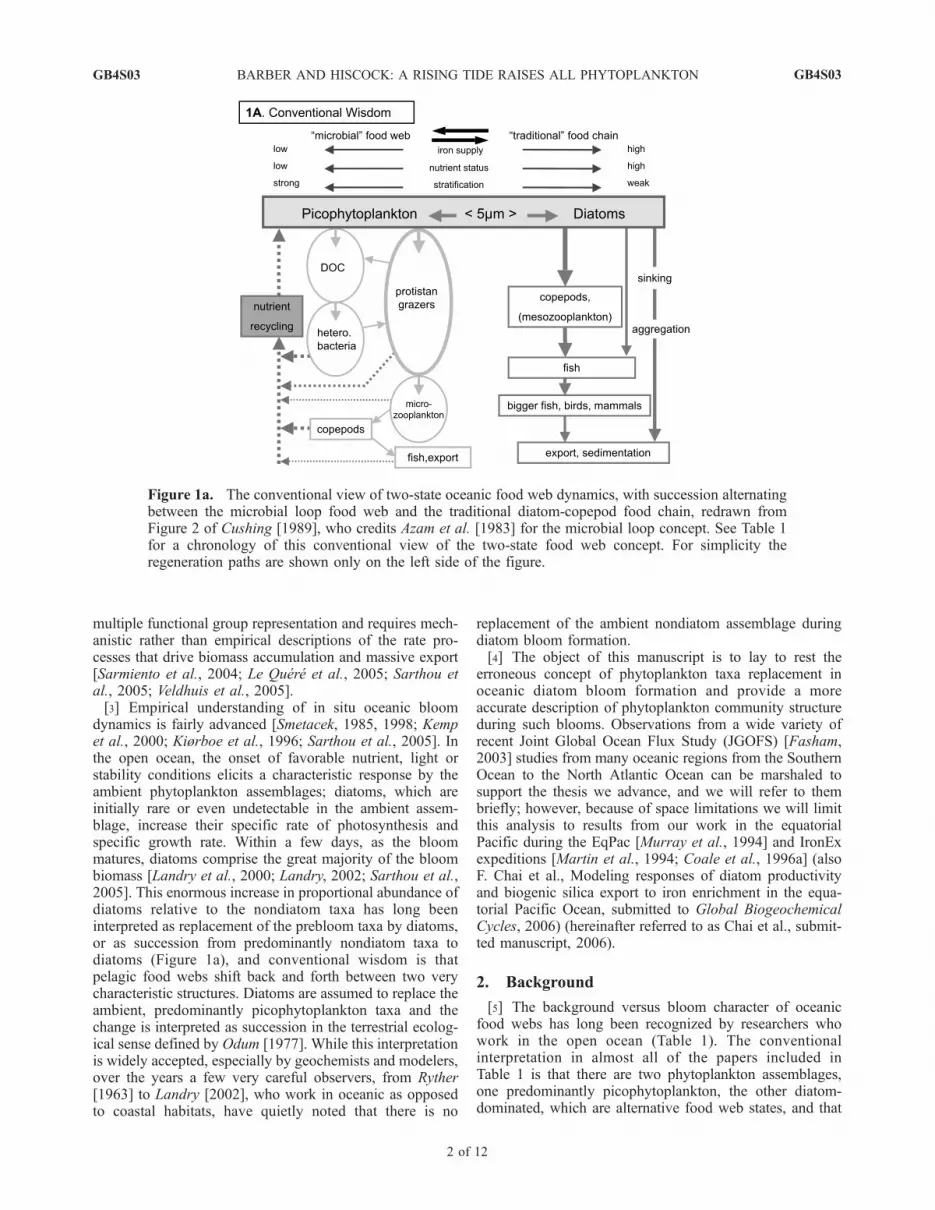
Figure 1a. The conventional view of two-state oceanic food web dynamics, with succession alternatingbetween the microbial loop food web and the traditional diatom-copepod food chain, redrawn fromFigure 2 of Cushing [1989], who credits Azam et al. [1983] for the microbial loop concept. See Table 1for a chronology of this conventional view of the two-state food web concept. For simplicity theregeneration paths are shown only on the left side of the figure.

GB4S03 BARBER AND HISCOCK: A RISING TIDE RAISES ALL PHYTOPLANKTON

2 of 12

GB4S03

environmental growth conditions, favorable or unfavorable,force a transition from one state to the other. In contrast tothis two-state concept, there is a parallel concept in aquaticecology in which the transition back and forth between

favorable and unfavorable conditions involves an orderlysuccession of dominance by various phytoplankton taxa.This sequence is clearly succession, as defined by Odum[1977], and it has been recognized for many years in aquatic

Figure 1b. The oceanic food web dynamics described in this report, showing the ambientpredominantly picophytoplankton food web that prevails during oligotrophic conditions. For simplicitythe regeneration paths are shown only on the left side of the figure.

Figure 1c. The oceanic food web dynamics described in this report, showing the complexpicophytoplankton and diatom food web structure that prevails in diatom-dominated blooms. Forsimplicity the regeneration paths are shown only on the left side of the figure.

GB4S03 BARBER AND HISCOCK: A RISING TIDE RAISES ALL PHYTOPLANKTON

3 of 12

GB4S03

settings [Hutchinson, 1941]. Margalef [1958, 1963, 1978]has provided the most elegant and widely accepted descrip-tion and explanation of the succession of eukaryotic phy-toplankton taxa that occurs in lakes, estuaries and coastalsettings where the sediment serves as a reservoir for theresting stages of various, mainly eukaryotic, phytoplanktontaxa that participate in this successional sequence. Heproposed that succession, driven by a kinetic energy subsidy(wind or tide) that both mixes nutrients upward and keepsdiatoms suspended in the euphotic zone, gives diatoms adouble growth advantage that allows them to replace non-diatom taxa. When the kinetic subsidy is removed, theopposite causality is at work: Nondiatom taxa replacediatoms, which are now nutrient limited, less buoyantbecause of nutrient stress, and with no upward kineticenergy subsidy [Waite et al., 1992a, 1992b; Kiørboe etal., 1993, 1996]. In the Margalef [1978] model, the non-diatom eukaryotic assemblage that is adapted to lownutrients and strong stratification is a climax condition,the last step in an orderly succession from the ‘‘pioneer’’community of diatoms [Margalef, 1967].[6] On close examination, succession and bloom forma-

tion in oceanic habitats appear to be two different processes.

Cushing [1989, p. 7], after a detailed discussion of physi-ological mechanisms that may drive succession, as used byMargalef, starts the next section of his paper with thefollowing:

‘‘A reasonable generalization might be that there are two mainforms of production cycle, that of the spring and autumn outbursts oftemperate waters and that of the stratified waters in the oligotrophicocean and the summer temperate seas. The latter system is in a quasisteady state in which numbers do not change much in time and as aconsequence the animals are dispersed. The traditional food chain isbased on the high amplitude production cycle with linked productionof herbivores and the aggregation of predators.

The production cycle in the oligotrophic ocean is in a quasi steadystate and the food chains are long and the organisms are dispersed. Thegreat fisheries of the world are based on the traditional food chain,rooted in the small diatoms (>5 mm in diameter) and their successors inthe spring outburst and, in the upwelling areas, the larger flagellates.’’

Cushing’s [1989] separation of succession from the two-state ‘‘production cycle’’ encourages us to proceed with ananalysis of the oceanic two-state transition process. Webelieve the ideas presented here are not in conflict with theconventional successional hypothesis of aquatic ecology,but stress that the oceanic transition from the ambient

Table 1. Representative Ideas About the Two-State Character of Open-Ocean Food Webs in Terms of Structure,

Forcing and Consequences, Showing That the Two-State Food Web Concept Has Been Recognized Widely, But

Interpreted By All But Ryther [1963] and Landry [2002] as a Replacement or Succession Process, as Illustrated

in Figure 1a

Microbial Food Web(Ambient Nondiatom

Food Web Assemblage)

Traditional Food Chain(Diatom-Dominated Bloom

Food Web) Reference

StructureNanoplankton net phytoplankton Yentsch and Ryther [1959]Flagellates flagellates + diatoms Ryther [1963]Nanoplankton net plankton Malone [1971]Dinoflagellates/mzooplankton diatoms/copepods Landry [1977]Flagellates diatoms Greve and Parsons [1977]Flagellates diatoms Parsons et al. [1978]m-eukaryotes/cyanobacteria small diatoms (>5mm, <20mm) Cushing [1989]Picophytoplankton (<5mm) picophyto. + diatoms (>20mm) Landry [2002]Protistan grazers protistan + crustacean grazers Landry [2002]Picophytoplankton picophytoplankton + diatoms this paper, Figures 1b and 1c

ForcingRegenerated nutrients new nutrients Dugdale and Goering [1967]Nutrient stress no nutrient stress Greve and Parsons [1977]Weakly stratified strongly stratified Cushing [1989]No surplus nitrate surplus nitrate Cushing [1989]Iron limited iron replete Landry et al. [1997]No surplus silicic acid surplus silicic acid Dugdale and Wilkerson [1998]

ConsequenceRegenerated production new production Dugdale and Goering [1967]Low fish yield high fish yield Ryther [1969]Equilibrium disequilibrium Landry [1977]Regenerative renewal Wangersky [1977]Modest fisheries the great fisheries Cushing [1989]Low fish yield high fish yield Iverson [1990]Low export massive export Waite et al. [1992a, 1992b]Nondiatoms diatoms Dugdale and Wilkerson [1998]Efficient recycling high export Dugdale and Wilkerson [1998]Balanced biomass large biomass pulse Landry [2002]Regenerated production regenerated + new production this paperRecycling more recycling + export this paper

GB4S03 BARBER AND HISCOCK: A RISING TIDE RAISES ALL PHYTOPLANKTON

4 of 12

GB4S03

oligotrophic assemblage to a high-biomass bloom does notappear to be succession in the sense that Margalef uses theterm.[7] The large proportional increase in diatom biomass that

characterizes bloom formation has led most, but not all, ofthe authors cited in Table 1 to the interpretation that diatomsreplace the nondiatom taxa. Before we show why webelieve that interpretation is erroneous, consider a commentby Ryther [1963, p. 25] (our italics):

‘‘What we find in Bermuda [at the oceanic Bermuda hydrographicstation] are two kinds of communities. One is a community which isadapted to living under very poor conditions, inhabited by smallflagellates which are able to swim around and snap up an occasionalphosphate ion, and so on. They make their own vitamins, and they areadapted to living under very unfavorable conditions, it seems.

Then, there is another community which suddenly appears whenthere is a turnover and the water is richer and there are vitaminspresent. These diatoms can grow very rapidly, and they are used toliving in lush conditions. They can outgrow or outstrip the other.Although the little flagellates hang on, they can never grow as fast,apparently, as the diatoms. It looks, therefore, as though they werebeing selected against, but, really, they are just staying at the samelevel all the time, and the diatoms come in and go out again.’’

Ryther [1963] clearly had a good intuitive sense of theadditive nature of bloom formation. More recently, Landry[2002, p. 32] makes the identical point while commentingon EqPac and IronEx results (our italics):

‘‘Phytoplankton biomass is further increased in this food web byadding more limiting nutrient, as was done during the IronEx IIfertilization (Figure 4). The result was a >40-fold increase in thebiomass of microphytoplankton (>20-mm size fraction), with a largelynegligible effect on smaller cells [Landry et al., 2000]. Suchobservations define the order in which successively larger phyto-plankton are added to the food web by ‘overprinting’ its relativelystable base of small cells [e.g. Chisholm, 1992; Landry et al., 1997].’’

3. Strategy and Methods

[8] The analysis presented here is based on work in theequatorial Pacific in wind-driven equatorial upwelling,tropical instability waves and other processes involvingfrontal dynamics that often produce favorable conditionsfor the beginning of a diatom bloom. In the fall of 1992during onset of a cool ENSO phase [Murray et al., 1994],there were numerous manifestations of short-lived diatomblooms driven by equatorially trapped processes thatupwelled nutrient-rich water [Lindley et al.,1995; Barberand Chavez, 1991; Bidigare and Ondrusek,1996; Landry etal., 1996; Latasa et al., 1997]. These equatorial waters arerich (�Ks) in nitrate and phosphate and have highlyvariable diatom abundance [Chavez et al., 1990, 1996].The limiting nutrients provided to the euphotic zone bythese physical processes were likely iron [Coale et al.,1996b], silicic acid [Dugdale and Wilkerson, 1998], or both.Figure 2 shows the increase of primary productivity anddiatom abundance at 2�N on a meridional section across theequatorial waveguide at 140�W. Productivity, diatom abun-dance, and particle flux through the 100-m-depth horizonare all maximal at 2�N where an instability front brought theiron-rich Equatorial Undercurrent into the euphotic zone[Barber et al., 1996; Johnson, 1996; Archer et al., 1997;Foley et al., 1997]. The euphotic zone diatom maximumclose to 2�N was associated with a maximum of freshphytodetritus on the sea floor about 4000 m below. ThisSeptember 1992 bloom at 140�W was so dense that it wasvisible to the space shuttle crew the same week we sampledthe front [Yoder et al., 1994; Archer et al., 1997; Barber etal., 1996]. Kemp and Baldauf [1993] have described lam-inated diatom deposits in the equatorial Pacific that look asthough they could have been laid down by a frontal bloomsimilar to the one we observed in 1992.[9] Analyses of pigment composition on equatorial trans-

ects in fall 1992 showed strong equatorial maxima in totalchlorophyll and diatom chlorophyll with no decrease inprokaryotic chlorophyll [Bidigare and Ondrusek, 1996,

Figure 2. Covariation of four properties related to diatomgrowth, export, and burial on a meridional transect acrossthe equator along 140�W longitude from 12�S to 12�N inthe Pacific Ocean during August and September 1992.(a) Primary productivity fromBarber et al. [1996]; (b) diatombiomass from Bidigare and Ondrusek [1996]; (c) carbonexport flux from Murray et al. [1996]; (d) phytodetritus onthe sea floor from Smith et al. [1996]. The maximum inprimary productivity, diatom biomass, and export produc-tivity at 2�N was associated with the cold side of aninstability wave front [Johnson, 1996; Archer et al.,1997;Barber et al., 1996], which was visible from space [Yoder etal., 1994].

GB4S03 BARBER AND HISCOCK: A RISING TIDE RAISES ALL PHYTOPLANKTON

5 of 12

GB4S03

Figures 8 and 9]. Landry et al. [1996, p. 871] show similardata from equatorial transects and summarize their obser-vations, ‘‘Picoplankton account for most of the chlorophyllbiomass and primary production in the central equatorialPacific. Nonetheless, their abundances and distributions arerelatively stable and conservative while other populations,

such as diatoms, respond more dramatically to environmen-tal forcing.’’[10] Quantifying growth responses driven by a natural

enrichment transient is difficult. The spatial and temporalexpressions of complex processes such as instability waves[Johnson, 1996] make it hard to determine when and wherethe enrichment started. To overcome this difficulty we have

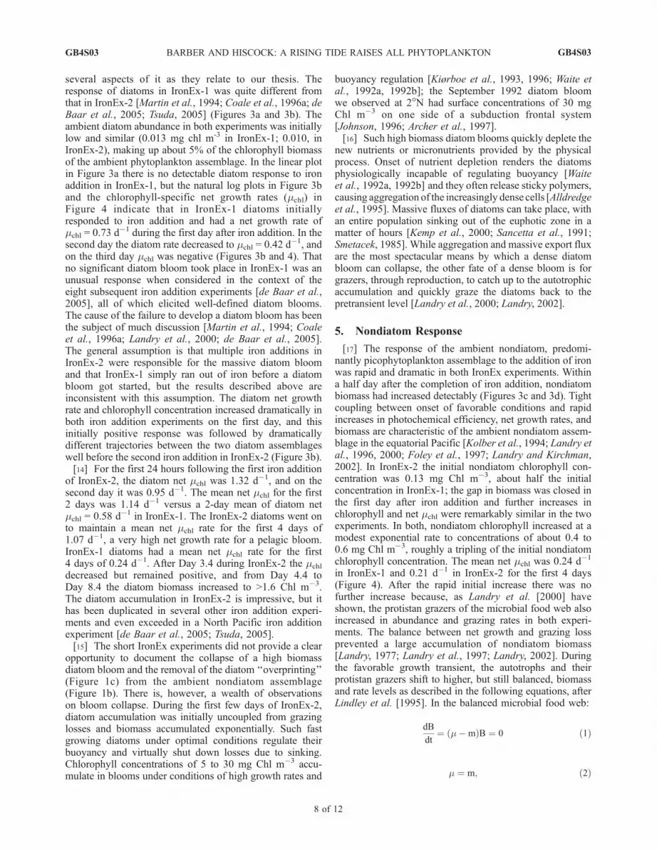
Figure 3. Time series of the increase of (a, b) diatom and (c, d) nondiatom chlorophyll followingaddition of iron in the 1993 IronEx-1 [Martin et al., 1994] and 1995 IronEx-2 [Coale et al., 1996a;Landry, 2002] in situ Fe addition experiments in the eastern equatorial Pacific Ocean. (e, f) Time series ofchlorophyll change in IronEx-2 for both diatoms and nondiatoms in one graph. Time series are shown inboth linear (Figures 3a, 3c, and 3e) and natural log (Figures 3b, 3d, and 3f) chlorophyll units todemonstrate different quantitative aspects of the initial responses to iron addition. The dashed lines inFigures 3c and 3e represent the new equilibrium chlorophyll value (Bnew � 0.46 mg Chl m�3) for theIronEx-2 nondiatom assemblage from Day 2.4 to Day 9.4. The vertical bars with diagonal lines showwhen iron was added: once in IronEx-1 (fine diagonal lines), and three times in IronEx-2 (fine and thickdiagonal lines). Robert R. Bidigare (University of Hawaii) provided the phytoplankton pigment data,which were determined by HPLC [Bidigare and Ondrusek, 1996] and converted to chlorophyllassociated with various taxa using pigment equations from Letelier et al. [1993].

GB4S03 BARBER AND HISCOCK: A RISING TIDE RAISES ALL PHYTOPLANKTON

6 of 12

GB4S03

analyzed the results of two iron addition experiments,IronEx-1 [Martin et al., 1994] and IronEx-2 [Coale et al.,1996a], where the time and place of the enrichment werecontrolled, making it possible to construct precise timeseries analyses. Lindley and Barber [1998] found that theambient phytoplankton response in the naturally iron-richisland wake of the Galapagos Islands was virtually identicalto the biological response in the IronEx experiments. On thebasis of these observations we propose that the open-oceaniron experiments are good surrogates for natural enrichmenttransients.[11] The observations in Figures 3 and 4 on the abun-

dance and chlorophyll-specific net growth rate of diatom,nondiatom, cyanophyte and prochlorophyte taxa weredetermined by high performance liquid chromatography(HPLC) pigment analyses done by Bidigare and Ondrusek[1996]; pigment analyses were converted to chlorophyllassociated with various taxa using pigment equations ofLetelier et al. [1993]. Samples for HPLC analysis werecollected from the surface and immediately filtered; thefilters were placed in liquid N2 for later HPLC analysis backat the lab. The time series of photochemical efficiency(Figure 5) was determined by Fast Repetition-Rate Fluo-rometry (FRRF) on 3-m water samples at frequent intervalsin the iron-enriched waters [Kolber et al., 1994; Behrenfeld

et al., 1996]. Together the HPLC and FRRF analyses are asuite of well-resolved spatial and temporal observations.

4. Diatom Response

[12] Diatom bloom initiation at onset of favorable envi-ronmental conditions is probably the most studied phenom-enon in oceanography [Gaarder and Gran, 1927; Riley,1946; Sverdrup, 1953;Ryther, 1969;Dugdale andWilkerson,1998; Hiscock et al., 2003; Sarthou et al., 2005]. It hascommanded much attention because of the well-establishedrelationship between diatom blooms and fish production[Iverson, 1990], which led Bostwick Ketchum to reviseIsaiah 40:6 this way, ‘‘All fish is diatom.’’ Together with thefish connection, diatom blooms are a major biologicalprocess for regulating the concentration of CO2 in Earth’satmosphere. Although it is prudent to say the precedingstatement is a hypothesis that is controversial, few ocean-ographers would deny that the formation of massive diatomblooms and their termination by rapid sinking to the seafloor have the potential, over geological timescales, tomodify the partitioning of carbon in the atmosphere-ocean-sediment system. The sedimentary record indicatesthat massive episodic burial has taken place [Kemp andBaldauf, 1993].[13] Although the environmental forcing of the diatom

growth response is well understood, we will describe

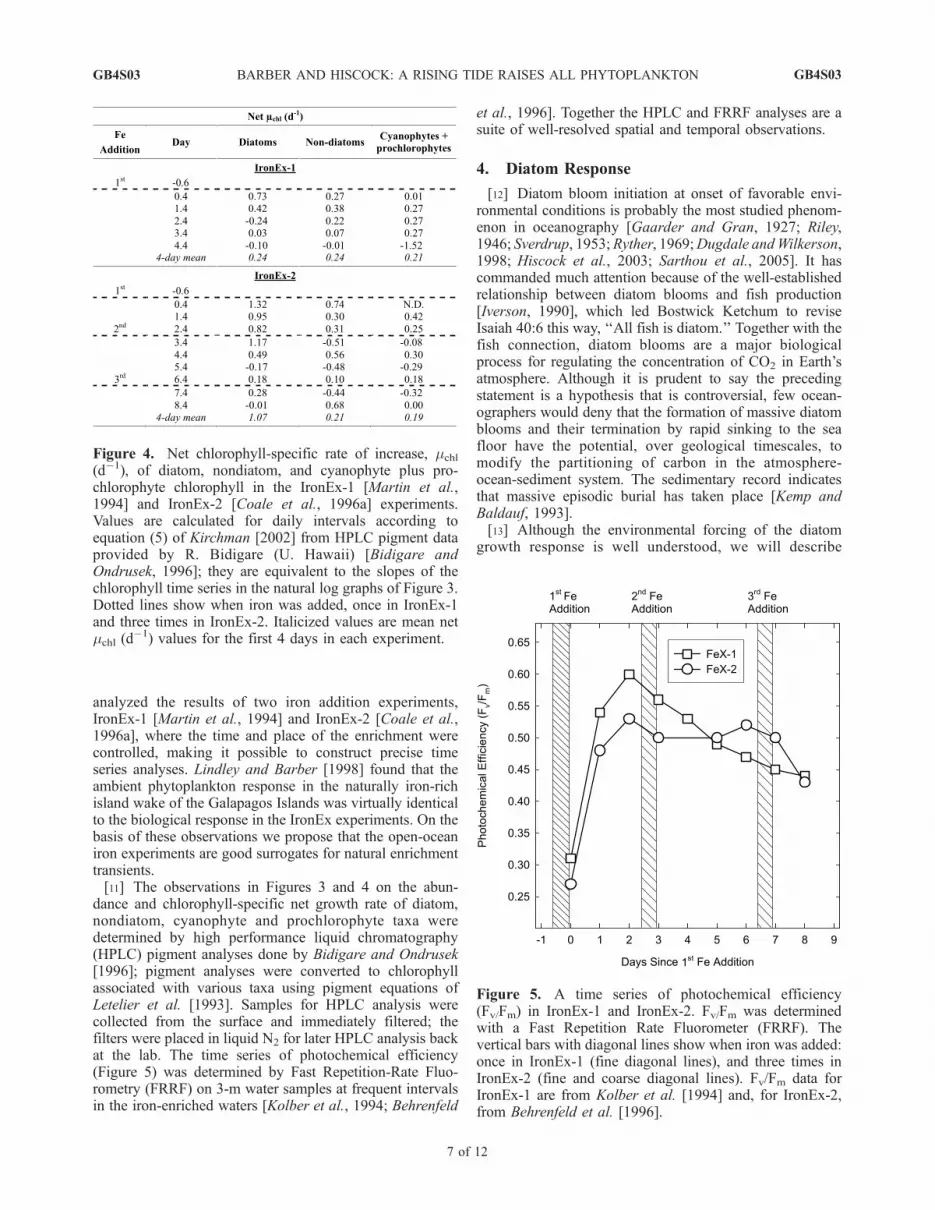
Figure 4. Net chlorophyll-specific rate of increase, mchl

(d�1), of diatom, nondiatom, and cyanophyte plus pro-chlorophyte chlorophyll in the IronEx-1 [Martin et al.,1994] and IronEx-2 [Coale et al., 1996a] experiments.Values are calculated for daily intervals according toequation (5) of Kirchman [2002] from HPLC pigment dataprovided by R. Bidigare (U. Hawaii) [Bidigare andOndrusek, 1996]; they are equivalent to the slopes of thechlorophyll time series in the natural log graphs of Figure 3.Dotted lines show when iron was added, once in IronEx-1and three times in IronEx-2. Italicized values are mean netmchl (d

�1) values for the first 4 days in each experiment.

Figure 5. A time series of photochemical efficiency(Fv/Fm) in IronEx-1 and IronEx-2. Fv/Fm was determinedwith a Fast Repetition Rate Fluorometer (FRRF). Thevertical bars with diagonal lines show when iron was added:once in IronEx-1 (fine diagonal lines), and three times inIronEx-2 (fine and coarse diagonal lines). Fv/Fm data forIronEx-1 are from Kolber et al. [1994] and, for IronEx-2,from Behrenfeld et al. [1996].

GB4S03 BARBER AND HISCOCK: A RISING TIDE RAISES ALL PHYTOPLANKTON

7 of 12

GB4S03

several aspects of it as they relate to our thesis. Theresponse of diatoms in IronEx-1 was quite different fromthat in IronEx-2 [Martin et al., 1994; Coale et al., 1996a; deBaar et al., 2005; Tsuda, 2005] (Figures 3a and 3b). Theambient diatom abundance in both experiments was initiallylow and similar (0.013 mg chl m-3 in IronEx-1; 0.010, inIronEx-2), making up about 5% of the chlorophyll biomassof the ambient phytoplankton assemblage. In the linear plotin Figure 3a there is no detectable diatom response to ironaddition in IronEx-1, but the natural log plots in Figure 3band the chlorophyll-specific net growth rates (mchl) inFigure 4 indicate that in IronEx-1 diatoms initiallyresponded to iron addition and had a net growth rate ofmchl = 0.73 d�1 during the first day after iron addition. In thesecond day the diatom rate decreased to mchl = 0.42 d�1, andon the third day mchl was negative (Figures 3b and 4). Thatno significant diatom bloom took place in IronEx-1 was anunusual response when considered in the context of theeight subsequent iron addition experiments [de Baar et al.,2005], all of which elicited well-defined diatom blooms.The cause of the failure to develop a diatom bloom has beenthe subject of much discussion [Martin et al., 1994; Coaleet al., 1996a; Landry et al., 2000; de Baar et al., 2005].The general assumption is that multiple iron additions inIronEx-2 were responsible for the massive diatom bloomand that IronEx-1 simply ran out of iron before a diatombloom got started, but the results described above areinconsistent with this assumption. The diatom net growthrate and chlorophyll concentration increased dramatically inboth iron addition experiments on the first day, and thisinitially positive response was followed by dramaticallydifferent trajectories between the two diatom assemblageswell before the second iron addition in IronEx-2 (Figure 3b).[14] For the first 24 hours following the first iron addition

of IronEx-2, the diatom net mchl was 1.32 d�1, and on thesecond day it was 0.95 d�1. The mean net mchl for the first2 days was 1.14 d�1 versus a 2-day mean of diatom netmchl = 0.58 d�1 in IronEx-1. The IronEx-2 diatoms went onto maintain a mean net mchl rate for the first 4 days of1.07 d�1, a very high net growth rate for a pelagic bloom.IronEx-1 diatoms had a mean net mchl rate for the first4 days of 0.24 d�1. After Day 3.4 during IronEx-2 the mchl

decreased but remained positive, and from Day 4.4 toDay 8.4 the diatom biomass increased to >1.6 Chl m�3.The diatom accumulation in IronEx-2 is impressive, but ithas been duplicated in several other iron addition experi-ments and even exceeded in a North Pacific iron additionexperiment [de Baar et al., 2005; Tsuda, 2005].[15] The short IronEx experiments did not provide a clear

opportunity to document the collapse of a high biomassdiatom bloom and the removal of the diatom ‘‘overprinting’’(Figure 1c) from the ambient nondiatom assemblage(Figure 1b). There is, however, a wealth of observationson bloom collapse. During the first few days of IronEx-2,diatom accumulation was initially uncoupled from grazinglosses and biomass accumulated exponentially. Such fastgrowing diatoms under optimal conditions regulate theirbuoyancy and virtually shut down losses due to sinking.Chlorophyll concentrations of 5 to 30 mg Chl m�3 accu-mulate in blooms under conditions of high growth rates and

buoyancy regulation [Kiørboe et al., 1993, 1996; Waite etal., 1992a, 1992b]; the September 1992 diatom bloomwe observed at 2�N had surface concentrations of 30 mgChl m�3 on one side of a subduction frontal system[Johnson, 1996; Archer et al., 1997].[16] Such high biomass diatom blooms quickly deplete the

new nutrients or micronutrients provided by the physicalprocess. Onset of nutrient depletion renders the diatomsphysiologically incapable of regulating buoyancy [Waiteet al., 1992a, 1992b] and they often release sticky polymers,causing aggregation of the increasingly dense cells [Alldredgeet al., 1995]. Massive fluxes of diatoms can take place, withan entire population sinking out of the euphotic zone in amatter of hours [Kemp et al., 2000; Sancetta et al., 1991;Smetacek, 1985]. While aggregation and massive export fluxare the most spectacular means by which a dense diatombloom can collapse, the other fate of a dense bloom is forgrazers, through reproduction, to catch up to the autotrophicaccumulation and quickly graze the diatoms back to thepretransient level [Landry et al., 2000; Landry, 2002].

5. Nondiatom Response

[17] The response of the ambient nondiatom, predomi-nantly picophytoplankton assemblage to the addition of ironwas rapid and dramatic in both IronEx experiments. Withina half day after the completion of iron addition, nondiatombiomass had increased detectably (Figures 3c and 3d). Tightcoupling between onset of favorable conditions and rapidincreases in photochemical efficiency, net growth rates, andbiomass are characteristic of the ambient nondiatom assem-blage in the equatorial Pacific [Kolber et al., 1994; Landry etal., 1996, 2000; Foley et al., 1997; Landry and Kirchman,2002]. In IronEx-2 the initial nondiatom chlorophyll con-centration was 0.13 mg Chl m�3, about half the initialconcentration in IronEx-1; the gap in biomass was closed inthe first day after iron addition and further increases inchlorophyll and net mchl were remarkably similar in the twoexperiments. In both, nondiatom chlorophyll increased at amodest exponential rate to concentrations of about 0.4 to0.6 mg Chl m�3, roughly a tripling of the initial nondiatomchlorophyll concentration. The mean net mchl was 0.24 d�1

in IronEx-1 and 0.21 d�1 in IronEx-2 for the first 4 days(Figure 4). After the rapid initial increase there was nofurther increase because, as Landry et al. [2000] haveshown, the protistan grazers of the microbial food web alsoincreased in abundance and grazing rates in both experi-ments. The balance between net growth and grazing lossprevented a large accumulation of nondiatom biomass[Landry, 1977; Landry et al., 1997; Landry, 2002]. Duringthe favorable growth transient, the autotrophs and theirprotistan grazers shift to higher, but still balanced, biomassand rate levels as described in the following equations, afterLindley et al. [1995]. In the balanced microbial food web:

dB

dt¼ m�mð ÞB ¼ 0 ð1Þ

m ¼ m; ð2Þ

GB4S03 BARBER AND HISCOCK: A RISING TIDE RAISES ALL PHYTOPLANKTON

8 of 12

GB4S03

where B is autotrophic picophytoplankton biomass, m is itsspecific growth rate, and m is the specific mortality loss ratedue to the sum of all loss processes. Since the majority ofloss in the microbial food web is due to grazing, we refer tothe sum of the losses as grazing loss. The balance betweenautotrophic growth rate and grazing (loss) rate requires thatm is density dependent,

m ¼ aB: ð3Þ

At steady state, the (loss) grazing constant a can be defined.Since m = m,

m ¼ aB ð4Þ

ma¼ B: ð5Þ

Under the influence of the favorable transient, m increases tomnew and biomass increases proportionally to Bnew,

mnew

Bnew

¼ a: ð6Þ

For the duration of the favorable transient, then, thisrelationship predicts a higher steady state biomass,increased steady state growth rate of small autotrophs, plusincreased grazing loss rate (mnew) [Lindley et al., 1995;Landry and Kirchman, 2002]. Protistan grazers in pelagicfood webs are almost always capable of preventing theformation of high biomass blooms of picophytoplankton;we know of only two reports of picophytoplankton blooms>1.5 mg chl m�3 in the open ocean [Morel, 1997; Bidigareet al., 1997].[18] In IronEx-1 and IronEx-2, nondiatom assemblages

reached the shifted-up biomass levels (Bnew) quickly. InIronEx-1 the iron-enriched parcel of water subductedbeneath a layer of water with ambient (low) iron concen-trations between Day 4 and Day 5; therefore, the surfaceHPLC pigment values after Day 4 are not representativeof the iron-stimulated community, making it impossible todetermine Bnew for IronEx-1 with any confidence. Figures 3cand 3d suggest that the nondiatom assemblages in the twoexperiments were following similar trajectories. In IronEx-2the mean Bnew value (0.46 mg Chl m�3) was reachedbetween Day 1.4 and Day 2.4, and was maintained for atleast 8 days with an oscillation of values between Days 2.4and 6.4 (Figure 3e) that suggested protistan grazers andautotrophs were settling into the new Bnew equilibriumvalue through a series of damped oscillations.[19] Chlorophyll-specific net growth rate calculations for

cyanophyte and prochlorophyte chlorophyll indicated thatthe nondiatom response was representative of the prokary-otic picophytoplankton response (Figure 4). For the first4 days of IronEx-1 the mean nondiatom net mchl = 0.24 d�1,the cyanophyte and prochlorophyte net mchl = 0.21 d�1; inIronEx-2 the net mchl values were similarly close, net mchl =0.21 d�1 for nondiatoms and 0.19 d�1 for cyanophytes andprochlorophytes. These results confirm that the ironresponse of the two major prokaryotic groups is similar to

the bulk nondiatom assemblage iron response; that is, theyincreased modestly in both biomass and chlorophyll-specificnet growth rate as also reported by Mann and Chisholm[2000].[20] Analysis of photochemical efficiency with the Fast

Repetition Rate Fluorometer (FRRF) has provided surpris-ing results from the two IronEx experiments (Figure 5).FRRF observations in IronEx-1 and IronEx-2 show thatambient Fv/Fm values in the equatorial Pacific are very low,around Fv/Fm = 0.3, indicating that ambient picophyto-plankton were iron limited when the IronEx experimentswere carried out (Figure 5). After iron addition in bothexperiments, Fv/Fm increased to high values in the first24 hours and up to maximal values after 48 hours. TheIronEx-1 and IronEx-2 response curves of photochemicalefficiency versus time were similar. In both experiments thephytoplankton assemblage in the first 24 and 48 hours wascomposed almost entirely of small phytoplankton. When themassive diatom accumulation did develop in IronEx-2, theFv/Fm curve remained similar to the response curve ofIronEx-1 where no diatoms were present.

6. Discussion

[21] The obvious questions generated by this analysis are(1) why is there no replacement of picophytoplankton bydiatoms when a physical or chemical transient abruptlyprovides favorable growth conditions, and (2) is this sig-nificant? First, why is there no succession or competitiveexclusion if the two groups are competing for a singlelimiting nutrient (iron) and other resources (light and macro-nutrients) are not limiting [Huisman and Weissing, 2000,2001]? Why do diatoms ‘‘overprint’’ the background pico-plankton rather than replace them? To understand this, it ishelpful to examine the strengths and inconsistencies ofconventional wisdom. The essence of the discussion onthe interactions between these two phytoplankton groups byMorel et al. [1991], Chisholm [1992], Raven [1998], andmany others (Table 1) is well summarized in the Ecumen-ical Hypothesis. The Ecumenical Hypothesis [Morel et al.,1991] states that large phytoplankton cells are more vulner-able to iron limitation than are picophytoplankton and thatthis vulnerability accounts for the dominance of picophy-toplankton in iron poor oceanic settings. Morel and hiscoauthors hypothesize that the photochemical efficiency ofpicophytoplankton is less sensitive to low iron rationsbecause small cells have lower cell quotas for iron, andlower half saturation constants for iron uptake enable themto take up iron rapidly at low concentrations [Price et al.,1994]. More importantly, the Ecumenical Hypothesis pre-dicts that after iron addition the photochemical efficiencyand growth rate of ambient picophytoplankton in highnutrient low chlorophyll (HNLC) waters will not increasemuch because the small cells are not strongly iron limitedand do not have the ability to respond to high levels of ironavailability by increasing photochemical efficiency. In con-trast, after iron addition large diatoms are predicted to showlarge increases in photochemical efficiency and growth ratebecause, with higher values of maximal uptake (Vmax) andmaximal growth rate (mmax) for iron [Coale et al., 1996b],

GB4S03 BARBER AND HISCOCK: A RISING TIDE RAISES ALL PHYTOPLANKTON

9 of 12

GB4S03

they can effectively exploit the newly available iron con-centrations (�4 nM) provided by iron addition experiments[Coale et al., 1996a; de Baar et al., 2005].[22] However, large diatoms are initially very rare (Figure 3)

and it takes several days for them to accumulate a sig-nificant biomass following iron addition. If the bulkincrease in photochemical efficiency resulting from ironaddition is being driven by the diatom response, as stated inthe Ecumenical Hypothesis, the increase should start slowlyand increase as diatoms begin to dominate the bloom’staxonomic composition. In situ FRRF observations ofphotochemical efficiency during both IronEx-1 andIronEx-2 [Kolber et al., 1994; Behrenfeld et al., 1996] areinconsistent with the Ecumenical Hypothesis; instead, theFRRF results show that photochemical efficiency increasedto maximal values during the first day of each experiment(Figure 5). We interpret this to indicate that the ambient,picophytoplankton were initially strongly iron limited andphysiologically capable of using the newly available iron. Inaddition, the IronEx-1 result, where only picophytoplanktonresponded to iron addition (Figure 3), shows that the rapidrate increase persisted for a week or longer in the picophy-toplankton dominated assemblage (Figure 5). Awareness ofthis initial strong positive response of ambient picophyto-plankton to iron addition (Figure 5) is critical to under-standing why diatoms do not displace picophytoplankton.[23] When iron suddenly becomes available in saturating

concentrations the two groups compete for available iron.Individual diatoms can take up iron that is present atsaturating concentrations much faster than picophytoplank-ton, but initially there are so few diatoms (Figure 3) that, asa population, they take up only a trivial proportion of thetotal available iron. In contrast, the uptake systems of thepicophytoplankton are saturated at their lower maximumuptake rates, yet most of the iron is initially partitioned intopicophytoplankton because of their overwhelming biomassdominance. As shown previously, the iron-limited ambientpicophytoplankton increased their photosynthetic efficiencywithin hours of iron addition (Figure 5). With excess ironavailable and saturated uptake rates, the ambient assem-blage of picophytoplankton shifts up to a new, highergrowth rate (mnew) (equation (6)), but because of efficientmicrograzing losses they cannot accumulate enough bio-mass to take up enough new iron to prevent the rapidlyincreasing diatoms from eventually taking up most of theiron. At the end of the bloom, in terms of photosyntheticefficiency, picophytoplankton are healthier than they werebefore iron addition, but over the course of the bloom theirbulk impact on the newly available iron is small. The keyissue is that as the bloom progresses, neither group out-competes the other: Picophytoplankton abundance is limitedby micrograzers, and diatoms compete with themselves.Picophytoplankton get all the iron they need to grow atmaximal rates; still, diatoms monopolize most of the newlyavailable iron. When diatom uptake drives down ironconcentration to diatom rate limiting concentrations, pico-phytoplankton, with lower ks values, are able to drive ironconcentration still lower. As the iron transient decays tobackground concentrations, ecological theory predicts thatpicophytoplankton with a lower requirement for iron very

effectively displace diatoms from the ambient assemblage[Huisman and Weissing, 2000, 2001].[24] As to the second question generated by this analysis,

is the paradigm change presented here quantitatively sig-nificant for carbon cycle modeling? Landry et al. [2006]argues that the increase in microbial cycling during bloomsmerits attention from modelers; his work in a variety ofocean settings as well as that of Eppley et al. [1979]indicates that bloom microbial production, grazing andrespiration can be enhanced several fold over backgroundcarbon cycling by this food web. A novel attempt atparameterizing the microbial food web was carried out byDenman and Pena [2002] and Denman [2003] using thesuggestion of Steele [1998] for including the picoplankton/micrograzer loop in an ocean ecosystem model of condi-tions at Ocean Station P in the subarctic North PacificOcean. Several ‘‘climate change’’ scenarios including theremoval of iron limitation were run to examine how themicrobial loop dynamics responded during the springbloom. Not surprisingly, the iron-enhanced run showed a29% increase in export flux across the 50-m-depth horizonfrom about 0.8 mol Nm�2 yr�1 to about 1.0 mol Nm�2 yr�1.In contrast, the export ratio, defined as the flux through the50-m depth divided by total primary productivity, decreasedin the iron-enhanced treatment; with iron limitation theexport ratio was 0.46, while in the iron-enhanced scenarioit decreased 32% to about 0.31. If absolute export fluxincreased with iron but the export ratio decreased by athird, there was a significant increase in recycling with iron.Direct flux measurements from the Southern Ocean ironaddition experiment [Buesseler et al., 2005] appear toconfirm the Denman [2003] model result: the absoluteexport flux increased with iron but the export ratiodecreased during the peak of bloom formation. These fieldand model results suggest that the new paradigm maycontribute to improved carbon cycle models.[25] The concept advanced here is also pertinent to the

15-year controversy sparked by Martin’s [1990] IronHypothesis [Chisholm, 1995]. Among other issues, thisdebate concerns the important environmental question, willengineered iron fertilization cause irreversible changes inthe pelagic ecosystem? Producing a strong export responseto iron enrichment requires both initial HNLC conditionsand a low background abundance of mesozooplankton,which allows diatom biomass to initially accumulate fasterthan ambient mesozooplankton can consume it [Landry etal., 2000]. Continuous iron fertilization will not produceefficient sequestration of carbon because as the mesozoo-plankton become abundant they can continuously graze andrecycle a large proportion of the newly produced diatombiomass in the surface layer. This increased grazing rateprevents the accumulation of the diatom biomass needed forefficient export. Therefore, efficient engineered carbonsequestration requires episodic Fe enrichment with a returnto the ambient picoplankton-dominated assemblagebetween enrichments.[26] Furthermore, iron enrichment drives consumption of

N, P and Si much faster than open ocean physical processescan resupply macronutrients (Chai et al., submitted manu-script, 2006), so continuous iron fertilization cannot effi-

GB4S03 BARBER AND HISCOCK: A RISING TIDE RAISES ALL PHYTOPLANKTON

10 of 12

GB4S03

ciently sequester carbon because the required HNLC con-ditions are not reestablished. Despite their ability to exploitnutrient transients, picophytoplankton are specialized forcompetition in resource limited environments [Raven, 1998].Both ecological theory [Huisman and Weissing, 2000, 2001]and modeling (Chai et al., submitted manuscript 2006)indicate that an iron-driven diatom bloom necessarilyforces an oscillation back to a picophytoplankton-dominatedassemblage, indicating that engineered iron fertilization willnot force an irreversible change in pelagic ecosystems toeither continuous diatom blooms or continuous picophyto-plankton dominance.

7. Conclusions

[27] Diatoms at very low abundances and the ambientpredominantly picophytoplankton assemblages of oligotro-phic open-ocean regions both respond positively to onset offavorable growth conditions. Diatoms grow fast, reducesinking loss by increasing buoyancy, and for a few daysaccumulate biomass faster than the mesozooplankton graz-ers can consume it. The picophytoplankton-protistan foodweb shifts to higher autotrophic growth rates and biomasslevels, but grazing also increases, so balance is maintainedand accumulation of picophytoplankton biomass is limited.New, slightly higher, equilibrium values of mnew, Bnew, andmnew are maintained in the microbial food web as long asthe favorable conditions persist.[28] Nondiatom autotrophs, especially picophytoplank-

ton, are more abundant in diatom blooms than in ambient,prebloom assemblages under oligotrophic conditions. Themicrobial food web in a bloom is more important quantita-tively to the carbon cycle than it is during backgroundsteady state conditions. There is more absolute recycling ofcarbon back to CO2 under bloom conditions than undernonbloom conditions, notwithstanding that carbon exportexceeds recycling by many fold in the bloom process.[29] Diversity and food web complexity are higher in the

episodic bloom than in the background steady state foodweb. The big biomass winners, the diatoms, do not replacethe ambient picophytoplankton assemblage; therefore thereis no succession in the ecological sense of the term duringbloom cycles.

[30] Acknowledgments. We thank the captains and crews of R/VThompson, R/V Iselin, R/V Revelle, R/V Melville, USCGS Polar Star, theshore support teams and our sea-going JGOFS colleagues who generouslyshared data and ideas with us. We especially thank Robert R. Bidigare ofthe University of Hawaii who has been a generous colleague and valuedmentor whose HPLC expertise has contributed to our work since 1992.Support was provided by the Division of Ocean Sciences and the Office ofPolar Programs of the U.S. National Science Foundation (NSF grants:OCE-9024373; OPP-9531981; OCE-9911441; OCE-0136270 and OCE-0312355 to R. T. B.).

ReferencesAlldredge, A., et al. (1995), Aggregation of a diatom bloom in a mesocosm:Bulk and individual particle optical measurements, Deep Sea Res., PartII, 42, 9–27.

Archer, D., et al. (1997), A meeting place of great ocean currents: Ship-board observations of a convergent front at 2�N in the Pacific, Deep SeaRes., Part II, 44, 1827–1849.

Azam, F., et al. (1983), The ecological role of water-column microbes in thesea, Mar. Ecol. Prog. Ser., 10, 257–263.

Barber, R. T., and F. P. Chavez (1991), Regulation of primary productivityrate in the equatorial Pacific Ocean, Limnol. Oceanogr., 36, 1803–1815.

Barber, R., et al. (1996), Primary productivity and its regulation in theequatorial Pacific during and following the 1991–92 El Nino, DeepSea Res., Part II, 43, 933–969.

Behrenfeld, M., et al. (1996), Confirmation of iron limitation of phyto-plankton photosynthesis in the equatorial Pacific Ocean, Nature, 383,508–511.

Bidigare, R., and M. Ondrusek (1996), Spatial and temporal variability ofphytoplankton pigment distributions in the central equatorial PacificOcean, Deep Sea Res., Part II, 43, 809–834.

Bidigare, R., et al. (1997), Observations of a Synechococcus-dominatedcyclonic eddy in open-oceanic waters of the Arabian Sea, Proc. SPIESoc. Opt. Eng., 2963, 260–265.

Bopp, L., et al. (2003), Dust impact on marine biota and atmospheric CO2

during glacial periods, Paleoceanography, 18(2), 1046, doi:10.1029/2002PA000810.

Boyd, P. W., and S. C. Doney (2002), Modeling regional responsesby marine pelagic ecosystems to global climate change, Geophys. Res.Lett., 29(16), 1806, doi:10.1029/2001GL014130.

Broecker, W. S., and T. F. Stocker (2006), The Holocene CO2 rise: Anthro-pogenic or natural?, Eos Trans. AGU, 87(3), 27–28.

Buesseler, K. O., et al. (2005), Particle export during the Southern OceanIron Experiment (SOFeX), Limnol. Oceanogr., 50, 311–327.

Chavez, F. P., et al. (1990), Phytoplankton taxa in relation to primaryproduction in the equatorial Pacific, Deep Sea Res., 37, 1733–1752.

Chavez, F. P., et al. (1996), Phytoplankton variability in the central andeastern tropical Pacific, Deep Sea Res., Part II, 43, 835–870.

Chisholm, S. W. (1992), Phytoplankton size, in Primary Productivity andBiogeochemical Cycles in the Sea, edited by P. G. Falkowski and A. D.Woodhead, pp. 213–237, Springer, New York.

Chisholm, S. W. (1995), The iron hypothesis: Basic research meets envir-onmental policy, Rev. Geophys., 33(S1), 1277–1286.

Coale, K., et al. (1996a), A massive phytoplankton bloom induced by anecosystem-scale iron fertilization experiment in the equatorial Pacific,Nature, 383, 495–501.

Coale, K., et al. (1996b), Control of community growth and export produc-tion by upwelled iron in the equatorial Pacific Ocean, Nature, 379, 621–624.

Cushing, D. (1989), A difference in structure between ecosystems instrongly stratified waters and in those that are only weakly stratified,J. Plankton Res., 11, 1–13.

de Baar, H. J. W., et al. (2005), Synthesis of iron fertilization experiments:From the Iron Age to the Age of Enlightenment, J. Geophys. Res., 110,C09S16, doi:10.1029/2004JC002601.

Denman, K. L. (2003), Modelling planktonic ecosystems: Parameterizingcomplexity, Prog. Oceanogr., 57, 429–452.

Denman, K. L., and M. A. Pena (2002), The response of two coupled 1-Dmixed layer/planktonic ecosystem models to climate change in the NESubarctic Pacific Ocean, Deep Sea Res., Part II, 49, 5739–5757.

Doney, S. C., et al. (2003), Global ocean carbon cycle modeling, in OceanBiogeochemistry: The Role of the Ocean Carbon Cycle in GlobalChange, edited by M. J. R. Fasham, pp. 216–238, Springer, New York.

Dugdale, R., and J. Goering (1967), Uptake of new and regenerated formsof nitrogen in primary productivity, Limnol. Oceanogr., 23, 196–206.

Dugdale, R., and F. Wilkerson (1998), Silicate regulation of new productionin the equatorial Pacific upwelling, Nature, 391, 270–273.

Eppley, R., et al. (1979), Nitrate and phytoplankton production in southernCalifornia coastal waters, Limnol. Oceanogr., 24, 483–494.

Falkowski, P. G., et al. (1998), Biogeochemical controls and feedbacks onocean primary production, Science, 281, 200–206.

Falkowski, P. G., et al. (2003), Phytoplankton and their role in primary,new, and export production, in Ocean Biogeochemistry: The Role of theOcean Carbon Cycle in Global Change, edited by M. J. R. Fasham,pp. 99–120, Springer, New York.

Fasham, M. J. R. (Ed.) (2003), Ocean Biogeochemistry: The Role of theOcean Carbon Cycle in Global Change, 297 pp., Springer, New York.

Foley, D., et al. (1997), Longwaves and primary productivity variations inthe equatorial Pacific at 0�, 140�W, Deep Sea Res., Part II, 44, 1801–1826.

Gaarder, T., and H. H. Gran (1927), Investigations of the production ofplankton in the Oslo Fjord, Rapp. P. V. Reun. Cons. Int. Exp. Mer, 42,1–48.

Gran, H. H. (1912), Pelagic plant life, in The Depths of the Ocean, editedby J. Murray and J. Hjort, pp. 307–387, MacMillan, New York.

Greve, W., and T. Parsons (1977), Photosynthesis and fish production:Hypothetical effects of climatic change and pollution, Helgol. Wiss.Meeresunters., 30, 66–72.

GB4S03 BARBER AND HISCOCK: A RISING TIDE RAISES ALL PHYTOPLANKTON

11 of 12

GB4S03

Hiscock, M. R., et al. (2003), Primary productivity and its regulation in thePacific sector of the Southern Ocean, Deep Sea Res., Part II, 50, 533–558.

Huisman, J., and F. J. Weissing (2000), Coexistence and competition,Nature, 407, 694.

Huisman, J., and F. J. Weissing (2001), Biological conditions foroscillations and chaos generated by multispecies competition, Ecology,82, 2682–2695.

Hutchinson, G. E. (1941), Ecological aspects of succession in naturalpopulations, Am. Nat., 75, 406–418.

Iverson, R. (1990), Control of marine fish production, Limnol. Oceanogr.,35, 1593–1604.

Johnson, E. (1996), A convergent instability wave front in the centraltropical Pacific, Deep Sea Res., Part II, 43, 753–778.

Kemp, A., and J. Baldauf (1993), Vast Neogene laminated diatommat depos-its from the eastern equatorial Pacific Ocean, Nature, 362, 141–144.

Kemp, A., et al. (2000), The ‘‘Fall dump’’: A new perspective on the role ofa ‘‘shade flora’’ in the annual cycle of diatom production and export flux,Deep Sea Res., Part II, 47, 2129–2154.

Kiørboe, T., et al. (1993), Turbulence, phytoplankton cell size, and thestructure of pelagic food webs, Adv. Mar. Biol., 26, 1–72.

Kiørboe, T., et al. (1996), Sedimentation of phytoplankton during a springdiatom bloom: Rates and mechanisms, J. Mar. Res., 54, 1123–1148.

Kirchman, D. L. (2002), Calculating microbial growth rates from data onproduction and standing stocks, Mar. Ecol. Prog. Ser., 233, 303–306.

Kohfeld, K., et al. (2005), Role of marine biology in glacial-interglacialCO2 cycles, Science, 308, 74–78.

Kolber, Z., et al. (1994), Iron limitation of phytoplankton photosynthesis inthe equatorial Pacific Ocean, Nature, 371, 145–149.

Landry, M. R. (1977), A review of important concepts in trophic organiza-tion of pelagic ecosystems, Helgol. Wiss. Meeresunters., 30, 8–17.

Landry, M. R. (2002), Integrating classical and microbial food web con-cepts: Evolving views from the open-ocean tropical Pacific, Hydrobiolo-gia, 480, 29–39.

Landry, M. R., and D. Kirchman (2002), Microbial community structureand variability in the tropical Pacific, Deep Sea Res., Part II, 49, 2669–2694.

Landry, M. R., et al. (1996), Abundances and distributions of picoplanktonpopulations in the central equatorial Pacific from 12�N to 12�S, 140�W,Deep Sea Res., Part II, 43, 871–890.

Landry, M. R., et al. (1997), Iron and grazing constraints on primary pro-duction in the central equatorial Pacific: An EqPac synthesis, Limnol.Oceanogr., 42, 405–418.

Landry, M. R., et al. (2000), Biological response to iron fertilization in theeastern equatorial Pacific (IronEx II): III. Dynamics of phytoplanktongrowth and microzooplankton grazing,Mar. Ecol. Prog. Ser., 201, 57–72.

Landry, M. R., et al. (2006), Microbial community dynamics during thedecline phase of a diatom bloom in a subtropical cyclonic eddy, paperpresented at 2006 Ocean Sciences Meeting, AGU, Honolulu, Hawaii.

Latasa, M., et al. (1997), Pigment-specific growth and grazing rates ofphytoplankton in the central equatorial Pacific, Limnol. Oceanogr., 42,289–298.

Le Quere, C., et al. (2005), Ecosystem dynamics based on plankton func-tional types for global ocean biogeochemistry models, Global ChangeBiol., 11, 1–25, doi:10.1111/j.1365-2486.2005.001004.x.

Letelier, R., et al. (1993), Temporal variability of phytoplankton communitystructure based on pigment analysis, Limnol. Oceanogr., 38, 1420–1437.

Lindley, S., and R. Barber (1998), Phytoplankton response to natural andartificial iron addition, Deep Sea Res., Part II, 45, 1135–1150.

Lindley, S., et al. (1995), Phytoplankton photosynthesis parameters along140�W in the equatorial Pacific, Deep Sea Res., Part II, 42, 441–463.

Longhurst, A. (1991), Role of the marine biosphere in the global carboncycle, Limnol. Oceanogr., 36, 1507–1526.

Malone, T. (1971), The relative importance of nanoplankton and net plank-ton as primary producers in tropical oceanic and neritic phytoplanktoncommunities, Limnol. Oceanogr., 16, 633–639.

Mann, E. L., and S. W. Chisholm (2000), Iron limits the cell division rate ofProchlorococcus in the eastern equatorial Pacific, Limnol. Oceanogr., 45,1067–1076.

Margalef, R. (1958), Temporal succession and spatial heterogeneity inphytoplankton, in Perspectives in Marine Biology, edited by A. A.Buzzato-Traverso, pp. 323–349, Univ. of Calif. Press, Berkeley.

Margalef, R. (1963), On certain unifying principles in ecology, Am. Nat.,97, 357–374.

Margalef, R. (1967), Some concepts relative to the organization ofplankton, Oceanogr. Mar. Biol. Annu. Rev., 5, 257–289.

Margalef, R. (1978), Life forms of phytoplankton as survival alternatives inan unstable environment, Oceanol. Acta, 1, 493–510.

Martin, J. (1990), Glacial-interglacial CO2 change: the iron hypothesis,Paleoceanography, 5, 1–13.

Martin, J., et al. (1994), Testing the iron hypothesis in ecosystems of theequatorial Pacific Ocean, Nature, 371, 123–129.

Morel, A. (1997), Consequences of a Synechococcus bloom upon theoptical properties of oceanic (case 1) waters, Limnol. Oceanogr., 42,1746–1754.

Morel, F. M., et al. (1991), Iron nutrition of phytoplankton and its possibleimportance in the ecology of ocean regions with high nutrient lowbiomass, Oceanography, 4, 56–61.

Murray, J., et al. (1994), Physical and biological controls on carbon cyclingin the equatorial Pacific, Science, 266, 58–65.

Murray, J., et al. (1996), Export flux of particulate organic carbon from thecentral equatorial Pacific determined using a combined driftingtrap-234Th approach, Deep Sea Res., Part II, 43, 1095–1132.

Odum, E. (1977), The emergence of ecology as a new integrative discipline,Science, 195, 1289–1293.

Parsons, T., et al. (1978), An experimental simulation of changes in diatomand flagellate blooms, J. Exp. Mar. Biol. Ecol., 32, 285–294.

Price, N. M., B. A. Ahner, and F. M. M. Morel (1994), The equatorialPacific Ocean: Grazer-controlled phytoplankton populations in an iron-limited system, Limnol. Oceanogr., 39, 520–534.

Raven, J. (1998), Small is beautiful: The picophytoplankton, Funct. Ecol.,12, 503–513.

Raven, J., and P. Falkowski (1999), Oceanic sinks for atmospheric CO2,Plant Cell Environ., 22, 742–755.

Riley, G. A. (1946), Factors controlling phytoplankton populations onGeorges Bank, J. Mar. Res., 5, 54–73.

Ryther, J. (1963), Components of ecosystems, in Marine Biology I, editedby G. Riley, p. 25, Am. Ins. of Biol. Sci., Washington, D. C.

Ryther, J. (1969), Photosynthesis and fish production in the sea, Science,166, 72–76.

Sancetta, C., et al. (1991), Massive fluxes of rhizosolenid diatoms: A com-mon occurrence?, Limnol. Oceanogr., 37, 1452–1457.

Sarmiento, J. L., et al. (2004), Response of ocean ecosystems to climatewarming, Global Biogeochem. Cycles, 18, GB3003, doi:10.1029/2003GB002134.

Sarthou, G., et al. (2005), Growth physiology and fate of diatoms in theocean: A review, J. Sea Res., 53, 25–42.

Smetacek, V. (1985), Role of sinking in diatom life history cycles, Mar.Biol., 84, 239–251.

Smetacek, V. (1998), Biological oceanography: Diatoms and the silicatefactor, Nature, 391, 224–225.

Smith, C., et al. (1996), Phytodetritus at the abyssal seafloor across 10� oflatitude in the central equatorial Pacific, Deep Sea Res., Part II, 43,1309–1338.

Steele, J. H. (1998), Incorporating the microbial loop in a simple planktonmodel, Proc. R. Soc. Ser. B, 265, 1771–1777.

Sverdrup, H. (1953), On conditions for the vernal blooming of phytoplank-ton, J. Cons. Cons. Int. Explor. Mer, 18, 287–295.

Tsuda, A. (2005), Two contrasting iron fertilization experiments in theWestern Subarctic Pacific, SOLAS News, 1, 7.

Veldhuis, M. J. W., et al. (2005), Picophytoplankton: A comparative studyof their biochemical composition and photosynthetic properties, J. SeaRes., 53, 7–24.

Waite, A., et al. (1992a), Spring bloom sedimentation in a subarctic eco-system: I. Nutrients and sinking, Mar. Biol., 114, 119–129.

Waite, A., et al. (1992b), Does energy control the sinking rates of marinediatoms?, Limnol. Oceanogr., 37, 468–477.

Wangersky, P. (1977), The role of particulate matter in the productivity ofsurface waters, Helgol. Wiss. Meeresunters., 30, 546–564.

Yentsch, C., and J. Ryther (1959), Relative significance of the net phyto-plankton and nanophytoplankton in the waters off Long Island Sound,J. Cons. Perm. Int. Explor. Mer, 24, 231–238.

Yoder, J., et al. (1994), A line in the sea, Nature, 371, 689–692.

�������������������������R. T. Barber, Nicholas School of the Environment and Earth Sciences,

Marine Laboratory, Duke University, 135 Duke Marine Lab Road,Beaufort, NC 28516, USA. (rbarber@duke.edu)M. R. Hiscock, Atmospheric and Oceanic Sciences Program, Princeton

University, PO Box CN710, Princeton, NJ 08544, USA.

GB4S03 BARBER AND HISCOCK: A RISING TIDE RAISES ALL PHYTOPLANKTON

12 of 12

GB4S03