a genetic algorithm with priority rules for solving job-shop scheduling problems

A Genetic Algorithm with Priority Rules forSolving Job-Shop Scheduling Problems

S.M. Kamrul Hasan, Ruhul Sarker, Daryl Essam, and David Cornforth

Abstract. The Job-Shop Scheduling Problem (JSSP) is one of the most difficult NP-hard combinatorial optimization problems. In this chapter, we consider JSSPs withan objective of minimizing makespan while satisfying a number of hard constraints.First, we develop a genetic algorithm (GA) based approach for solving JSSPs. Wethen introduce a number of priority rules to improve the performance of GA, suchas partial re-ordering, gap reduction, and restricted swapping. The addition of theserules results in a new hybrid GA algorithm that is clearly superior to other well-known algorithms appearing in the literature. Results show that this new algorithmobtained optimal solutions for 27 out of 40 benchmark problems. It thus makes asignificantly new contribution to the research into solving JSSPs.

1 Introduction

In this chapter, we present a new hybrid algorithm for solving the Job-Shop Schedul-ing Problems (JSSPs) that is demonstrably superior to other well-known algorithms.The JSSP is a common problem in the manufacturing industry. A classical JSSP in-volves a combination of N jobs and M machines. Each job consists of a set of opera-tions that has to be processed on a set of known machines, where each operation hasa known processing time. A schedule is a complete set of operations required by ajob, to be performed on different machines in a given order. In addition, the processmay need to satisfy other constraints. The total time between the start of the first

S.M. Kamrul Hasan and Ruhul Sarker and Daryl EssamSchool of IT&EE, University of New South Wales at the Australian Defence Force Academy,Northcott Drive, Canberra, ACT 2600, Australiae-mail: kamrul,r.sarker,[email protected]

David CornforthDivision of Energy Technology, Commonwealth Scientific and Industrial ResearchOrganization, Murray Dwyer Circuit, Mayfield West, NSW 2304, Australiae-mail: [email protected]

kamrul,r.sarker,[email protected]

[email protected]

56 S.M.K. Hasan et al.

operation and the end of the last operation, is termed as the makespan. Makespanminimisation is widely used as an objective in solving JSSPs [2, 8, 16, 37, 47, 50,51]. A feasible schedule contains no conflicts such as (i) no more than one oper-ation of any job can be executed simultaneously and (ii) no machine can processmore than one operation at the same time. The schedules are generated on the basisof a predefined sequence of machines and the given order of job operations.

The JSSPs are widely acknowledged as one of the most difficult NP-completeproblems [22, 23, 35]. They are also well-known for their practical applicationsin many manufacturing industries. Over the last few decades, a good number ofalgorithms have been developed to solve JSSPs. However, no single algorithm cansolve all kinds of JSSPs optimally (or near optimally) within a reasonable time limit.Thus, there is scope to analyze the difficulties of JSSPs as well as to design improvedalgorithms that may be able to solve them.

In this work, we start by examining the performance of the traditional GA (TGA)for solving JSSPs. Each individual represents a particular schedule and the indi-viduals are represented by binary chromosomes. After reproduction, any infeasibleindividual is repaired to make it feasible. The phenotype representation of the prob-lem is a matrix of N ×M numbers where each row represents the sequence of jobsfor a given machine. We apply both genotype and phenotype representations to an-alyze the schedules. The binary genotype is effective for the simple crossover andmutation techniques. After analyzing the traditional GA solutions, we realize thatthe solutions could be improved further by applying simple rules or local searches.So, we introduce three new priority rules to improve the performance of traditionalGA, namely: partial reordering (PR), gap reduction (GR), and restricted swapping(RS). These priority rules are integrated as a component of TGA. The actions ofthese rules will be accepted if and only if they improve the solution. The details ofthese priority rules are discussed in a section later in this chapter. We also imple-ment our GA incorporating different combinations of these priority rules. For easeof explanation, in this chapter, we designate these as PR with GA, GR with GAand GR plus RS with GA, as PR-GA, GR-GA, and GR-RS-GA respectively. To testthe performance of our proposed algorithms, we solve 40 of the benchmark prob-lems originally presented in Lawrence [33]. The proposed priority rules improvedthe performance of traditional GAs for solving JSSPs. Among the GAs with priorityrules, GR-RS-GA was the best performing algorithm. It obtained optimal solutionsfor 27 out of 40 test problems. The overall performance of GR-RS-GA is better thanmany key JSSP algorithms that appear in the literature. The current version of ouralgorithm is much refined than our earlier version. The initial and intermediate de-velopments of the algorithm, with limited experimentation, can be found in Hasanet al. [28, 29, 30].

The rest of this chapter is organized as follows. After the introduction, a briefreview of approaches for solving JSSPs is provided. Section 3 defines the JSSP con-sidered in this research. Section 4 discusses traditional GA approaches for solvingJSSPs, including chromosome representations used for JSSPs, and ways of han-dling infeasibility in JSSPs. Section 5 introduces new priority rules for improvingthe performance of traditional GA. Section 6 presents the proposed algorithms and

A Genetic Algorithm with Priority Rules for Solving JSSP 57

implementation aspects. Section 7 shows the experimental results and the necessarystatistical analysis used to measure the performance of the algorithms. Finally, theconclusions and comments on future research are presented.

2 Solving JSSP: A Brief Review

Scheduling is a very old and widely accepted combinatorial optimization problem.Conway [14] in late 60s, Baker [5] in mid 70s, and French [21] in early 80s. showedmany different ways of solving various scheduling problems, which were frequentlyused in later periods. Job-shop scheduling is one of those challenging optimizationproblems. A JSSP consists of N jobs, where each job is composed of a finite numberof operations. There are M machines, where each machine is capable of executinga set of operations Ok, where k is the machine index. The size of the solution spacefor such a problem is (n1)!(n2)!(n3)...(nk)...(nM−1)!(nM), where nk is the numberof operations executable by machine k. For equal number of operations in eachmachine, this is equal to (N!)M . Of course, many solutions are infeasible, and morethan one optimal solutions may exist. As the number of alternative solutions growsat a much faster rate than the number of jobs and the number of machines, it isinfeasible to evaluate all solutions (i.e., complete enumeration) even for a reasonablysized practical JSSP. The feasible solutions can be classified as semi-active, active,and non-delay schedules [44]. The set of non-delay schedules is a complete subsetof the set of active schedules, where the active set itself is a complete subset of theset of semi-active schedules [27]. In the semi-active schedules, no operation canbe locally shifted to the left, where in the active schedules, no left shift is possibleeither locally or globally. These two kinds of schedules may contain machine delay.Solutions having zero machine delay time are termed as the non-delay schedules. Inour algorithms, we force the solutions to be in the non-delay scheduling region.

In the early stages, Akers and Friedman [3], and Giffler and Thompson [24] ex-plored only a subset of the alternative solutions in order to suggest acceptable sched-ules. Although such an approach was computationally expensive, it could solve theproblems much quicker than a human. Later, the branch-and-bound (B&B) algo-rithm became very popular for solving JSSPs. It uses the concept of omitting a sub-set of solutions comprising those, that were out of bounds [4, 10, 12]. Among them,Carlier and Pinson [12] solved a 10×10 JSSP optimally for the first time, a problemthat was proposed in 1963 by Muth and Thompson [36]. They considered the N×MJSSP as M one-machine problems and evaluated the best preemptive solution foreach machine. Their algorithm relaxed the constraints on all other machines exceptthe one under consideration. The concept of converting a M machines problem toa one-machine problem was also found in Emmons [19] and Carlier [11]. As thecomplexity of this algorithm is directly dependent on the number of machines, it isnot computationally efficient for large scale problems.

Although the above algorithms can achieve optimum or near optimum makespan,they are computationally expensive, infeasible for large problems, even with cur-rent computational power. For this reason, numerous heuristic and meta-heuristic


approaches have been proposed in the last few decades. These approaches do notguarantee optimality, but provide a good quality solution within a reasonable pe-riod of time. Examples of such approaches applied to JSSPs are genetic algorithm(GA) [7, 16, 18, 38, 51], tabu search (TS) [6, 17], shifting bottleneck (SB) [2, 15],greedy randomized adaptive search procedure (GRASP) [8], and simulated anneal-ing (SA) [32]. The vast majority of this work focuses on the static JSSP, where thereare a fixed number of machines and jobs. However, many practical problems can beflexible in terms of the flexibility of constraints, availability of jobs, etc., and thiscan make solutions even more difficult to obtain. For example, Kacem et al. [31]demonstrated a localization method and an evolutionary approach, while Zribiet al. [53] proposed a hierarchical method for solving flexible JSSPs (FJSSPs).

Over the last few decades, a substantial amount of work aimed at solving JSSPsby using genetic algorithms and hybrid genetic algorithms has been reported.Lawrence [34] explained how a genetic algorithm can be applied for solving JSSPs.It is very common to improve the performance of the GA by incorporating differentsearch and heuristic techniques, and this approach is readily applied to solving theJSSP using a GA. For example, after applying the crossover operator, Shigenobuet al. [43] used the G&T method to build active schedules (i.e., schedules havingno unnecessary machine idle time). The G&T method, which is named after Gifflerand Thompson [24], is an enumeration technique that explores only a subset of thefeasible schedules. These feasible schedules are recognized as active schedules. Theactive schedules in turn convert to a subset of optimal schedules. However, the G&Tmethod ensures only the activeness, and not the optimality, as finding the optimalsolution for larger problems is expensive. Park et al. [41] used the G&T method togenerate a set of good and diverse initial solutions. Croce et al. [16] focused on theactiveness of the schedules and proposed a genetic algorithm based approach forsolving JSSPs.

Aarts et al. [1] provided a comparative analysis of different methods, such asmulti-stage iterative improvement (MSII), threshold acceptance (TA), simulated an-nealing (SA) and GA with neighborhood search, that can be useful for solvingJSSPs. Ombuki and Ventresca [38] reported two different approaches for solvingJSSPs. The first approach is based on a simple GA with a task assignment scheme(TAS), where a task is assigned to the earliest free machine, taking preemption, con-currency and machine idle time into account. TAS works well for those solutionswhere only one operation waits for each machine at any instance. Otherwise somepriority-rules may be used to improve the performance. In the second approach,the authors incorporated a local search (LS) mutator to improve the quality of so-lutions obtained by GA with TAS, though they reported that it does not guaranteeany improvement. The local search looks for the best makespan by swapping eachconsecutive pair of a solution. It is computationally very expensive and does notwork when more than one swapping is necessary. For this reason, they hybridizedthe genetic approach by replacing its local search by a simple tabu search proposedby Glover [25]. It is still expensive in terms of computation and memory, and isnot good enough to identify required multiple swapping. Gonalves et al. [27] alsoapplied two-exchange local search over the genetic algorithms. The search allows


up to two swaps at once to improve the fitness. The authors considered the set of ac-tive and non-delay schedules in two of their approaches. They also proposed param-eterized active schedules which may have a machine delay up to a certain threshold.Tsai and Lin [46] applied a single-swap local search which tries to swap each andevery consecutive pair of a selected solution and accepts the new solution if it im-proves the fitness. But in major cases, more than one swap is necessary to improvethe fitness.

Xing et al. [49] implemented an adaptive GA where the reproduction parametersare adapted by the algorithm itself. They proposed to use variable crossover andmutation probability which are calculated by an exponential function. The functionis a factor of the best and average fitness of the current generation. Yang et al. [52]proposed a similar approach for solving JSSPs. They considered the current num-ber of generation as another factor to calculate the reproduction parameters. As thegeneration progresses, the rate of mutation is increased. Genetic programming (GP)was integrated with GA for solving JSSPs by Werner et al. [48]. This technique hashigher time complexity as for a single generation of GP, GA runs for a hundreds ofgenerations.

The Shifting Bottleneck (SB) approach, which is derived from the concept ofone-machine scheduling, has been using by some researchers for solving JSSP[11, 12, 19]. It starts by arranging the machines according to a specific order, thenidentifies the first bottleneck machine and schedules it optimally. Then, it selectsthe next machine in the order and updates the starting time of the jobs that havealready been scheduled. The main purpose of this technique is to identify the bestorder of the machines. The most frequently used strategy is to rearrange the ma-chines according to the criticalness of the machines as identified by the longestprocessing time. Carlier and Pinson [12] proposed to apply B&B for one machineschedules, which is effective only for independent jobs. However there might bea path that exists between two operations of a job that creates a dependency. Inthat case, Dauzere-Peres and Lasserre [15] proposed to increase the release date ofsome unselected jobs to reduce the waiting time between the dependent jobs. Adamset al. [2] also focused on the importance of the appropriate ordering of machines inthe SB heuristic for JSSP. The main demerit of this heuristic is that it considers onlythe local information, i.e., only the status of the current and previously consideredmachines, which may not be effective for all cases.

Feo et al. [20] proposed a metaheuristic method, known as greedy randomizedadaptive search procedure (GRASP) which was used later by Binato et al. [8], forsolving JSSPs, this consists of two phases: construction where feasible solutionsare built, and local search where the neighborhood solutions are explored. In theconstruction phase, the authors proposed to maintain a restricted candidature list(RCL) consisting of all possible schedulable operations, to select an appropriate op-eration to schedule. Different probability distributions are found for this selection inBresina [9]. The authors proposed to select the operation which gives the minimumincrement of schedule time from that instance. This technique may not work in allcases, as it reduces the schedule time for one machine and may delay some oper-ations in other machines. They proposed a local search that identifies the longest


path in the disjunctive graph and swaps the critical paths to improve the makespan.GRASP has a problem that it does not take into account any information from theprevious iterations. To address this, the authors proposed an intensification tech-nique which keeps track of the elite solutions (e.g., having better fitness value) andincludes new solutions in the record if they are better than the worst from the elitelist. They also applied the proximate optimality principle (POP) to avoid the errorin scheduling early in the construction process in such a way that may lead to errorsin the following operations. The new approach proposed in this chapter overcomesthese shortcomings by utilising heuristics that effectively comprise a local searchtechnique, while maintaining an elite group.

3 Problem Definition

The standard job-shop scheduling problem makes the following assumptions: Eachjob consists of a finite number of operations.

• The processing time for each operation using a particular machine is defined.• There is a pre-defined sequence of operations that has to be maintained to com-

plete each job.• Delivery times of the products are undefined.• There is no setup or tardiness cost.• A machine can process only one job at a time.• Each job is performed on each machine only once.• No machine can deal with more than one type of task.• The system cannot be interrupted until each operation of each job is finished.• No machine can halt a job and start another job before finishing the previous one.• Each and every machine has full efficiency.

The objective of the problem is the minimization of the maximum time taken tocomplete each and every operation, while satisfying the machining constraints andthe required operational sequence of each job. In this research, we develop threedifferent algorithms for solving JSSPs. These algorithms are briefly discussed in thenext three subsections of the next section.

4 Job-Shop Scheduling with Genetic Algorithm

In this chapter, we consider the minimization of makespan as the objective of JSSPs.According to the problem definition, the sequence of machine use (this is also thesequence of operations) by each job is given. In this case, if we know either thestart or end time of each operation, we can calculate the makespan for each job andhence generate the whole schedule. In JSSPs, the main aim is to find the sequenceof jobs to be operated on each machine that minimizes the overall makespan. Thechromosome representation is an important issue in solving JSSPs using GAs. Wediscuss the representation aspect in the next section.


4.1 Chromosome Representation

In solving JSSPs using GAs, the chromosome of each individual usually comprisesthe schedule. Chromosomes can be represented by binary, integer or real numbers.Some popular representations for solving JSSPs are: operation based, job based,preference-list based, priority-rule based, and job pair-relationship based represen-tations [42]. A list of representations commonly used for JSSPs can be found in thesurvey of Cheng et al. [13]. In the operation-based representation, each gene standsfor a sequence of operations where every integer numbers in a gene represents a jobID. The first occurrence of a job ID in a chromosome stands for the first operationof that job in a defined machine. Suppose for a 3×3 JSSP; a chromosome may berepresented as ‖211323321‖ where the first number ’2’ means the first operationof job j2(O21), similarly the second number ’1’ indicates the first operation of jobj1(O11), the third number ’1’ indicates the second operation (as second appearanceof the number ’1’) of job j1(O12) and so on. Then the operations can be read fromthe chromosome as O21O11O12... and so on, where O ji represents the ith operationof the job j [42]. As the job processing time is known, it is possible to construct thecomplete schedule from the chromosome information.

In the job-based representation, both the machine sequences and job sequencesare necessary to represent a solution. Here, the first job is scheduled first. Moreover,the sequence of operations of each job is determined from the machine sequence.In this representation, there should be two strings of same length; one is the chro-mosome and another is the machine sequences. Each number in the chromosomerepresents a machine ID and the numbers in machine sequence represent the job ID.For example, if the chromosome is ‖322112313‖ and the sequence of machines is‖213122133‖, the number 2 (which is job 2) occurs three times in the chromosome.Here, the corresponding values in the machine field are 1, 3 and 2. That means thatthe sequence of the job j2 is m1m3m2.

In the preference list-based representation, the chromosome represents the pref-erences of each job. There are M sub-chromosomes in each chromosome where eachsub-chromosome represents the preference of the jobs on that machine. Suppose, ifthe chromosome looks like ‖312123321‖, it means that the first preferential jobs onmachines m1, m2 and m3 are jobs j3, j1 and j3 respectively.

We select the job pair-relationship based representation for the genotype, asin [37, 39, 50, 51], due to the flexibility of applying genetic operators to it. Inthis representation, a chromosome is symbolized by a binary string, where eachbit stands for the order of a job pair (u,v) for a particular machine m.

For a chromosome Ci

Ci(m,u,v) =

1 if the job ju preceeds the job jv in machine m

0 otherwise(1)

This means that in the chromosome representing the individual i, if the relevantbit for job ju and job jv for machine m is 1, ju must be processed before jv in


machine m. The job having the maximum number of 1s is the highest priority jobfor that machine. The length of each chromosome is

l = M× (N −1)×N/2 (2)

where N stands for the number of jobs, and M for the number of machines. Thus, lis the number of pairs formed by a job with any other job. This binary string acts asthe genotype of individuals. It is possible to construct a phenotype which is the jobsequence for each machine. This construction is described in Table 1. This repre-sentation is helpful if the conventional crossover and mutation techniques are used.We use this representation for the flexibility of applying simple reproduction oper-ators. More representations can be found in the survey [13]. As this chromosomedoes not contribute to the evaluation process, it does not affect the speed of evalu-ation. Like some other crossovers, such as partially matched crossover (PMX) andorder crossover (OX) that operate only on the phenotypes, the operation-based orjob-based representation can be used instead of the binary job-pair relation basedrepresentation. We also use the constructed phenotype as the chromosome on whichto apply some other heuristic operators that are discussed later.

In this algorithm, we map the phenotype directly from the binary string, i.e.,the chromosome, and perform the simple two-point crossover and mutation on it.For this, the crossover points are selected randomly. After applying the operators,as these reproduction operators may produce an infeasible solution [37, 50, 51], weperform the following repairing techniques: local and global harmonization, in orderto make this solution feasible. The solutions that remain feasible or unaffected bythe reproduction operations need not to be involved in this repairing. We also applyheuristic operators on the constructed phenotype, and these are discussed later.

4.2 Local Harmonization

This is the technique of constructing (which can be recognized as decoding) thephenotype (i.e., the sequence of operations for each machine) from the binary geno-type. M tables are formed from a chromosome of length l as described in Eq. (2).Each of the tables is of N×N size which reflects the relationship between the corre-sponding jobs of every job pair which contains only binary values. The job havingthe maximum number of 1s’ represents the most preferred job having the highestpriority score. These jobs are then rearranged according to their own priorities. Ta-ble 1 shows the way to construct the phenotype from the genotype by applying localharmonization.

Table 1.a represents the binary chromosome (for a 3 jobs and 3 machines prob-lem) where each bit represents the preference of one job with respect to another jobin the corresponding machine. The third row shows the machine pairs in a givenorder. The second row indicates the order of the machines for the first job of thepair shown in the third row. The first bit is 1, which means that job j1 will appearbefore job j2 in machine m1. Table 1.b.1, Table 1.b.2 and Table 1.b.3 represent the


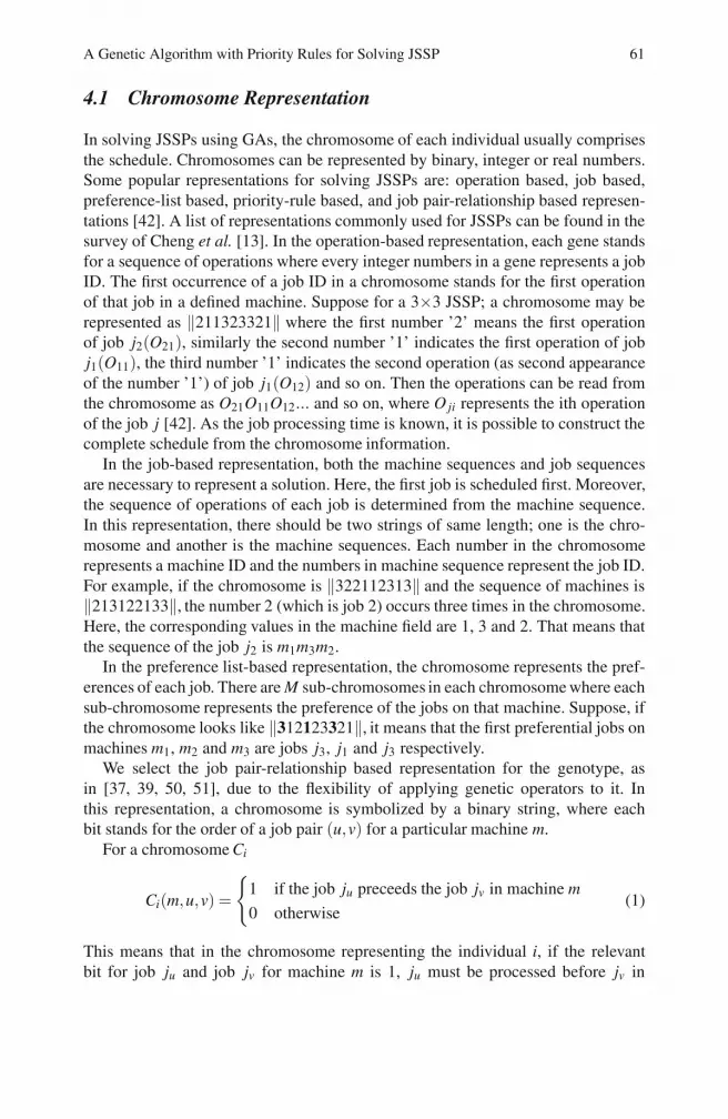
Table 1 Construction of the phenotype from the Binary genotype and Pre-defined Sequences

1 0 1 0 0 1 1 0 0m1 m3 m2 m1 m3 m2 m2 m1 m3

j1 − j2 j1 − j3 j2 − j3

1.a

j1 j2 j3 S j1 j2 j3 S j1 j2 j3 S

j1 * 1 0 1 j1 * 1 1 2 j1 * 0 0 0j2 0 * 0 0 j2 0 * 1 1 j2 1 * 0 1j3 1 1 * 2 j3 0 0 * 0 j3 1 1 * 2

1.b.1 1.b.2 1.b.3

jo1 jo2 jo3 mt1 mt2 mt3

j1 m1 m3 m2 m1 j3 j1 j2j2 m2 m1 m3 m2 j1 j2 j3j3 m1 m3 m2 m3 j3 j2 j1

1.c 1.d

job pair based relationship in machines m1, m2 and m3 respectively, as mentioned inEq. (1). In Table 1.b.1, the ’1’ in cell j1 − j2 indicates that job j1 will appear beforejob j2 in machine m1. Similarly, the ’0’ in cell j1 − j3 indicates that job j1 will notappear before job j3 in machine m1. In the same Table 1.b, column S represents thepriority of each job, which is the row sum of all the 1s for the job presented in eachrow. A higher number represents a higher priority because it precedes all other jobs.So for machine m1, job j3 has the highest priority. If more than one job has equalpriority in a given machine, a repairing technique modifies the order of these jobsto introduce different priorities. Consider a situation where the order of jobs for agiven machine is j1 − j2, j2 − j3, and j3 − j1. This will provide S = 1 for all jobs inthat machine. By swapping the content of cells j1 − j3, and j3 − j1, it would provideS = 2, 1 and 0 for jobs j1, j2, and j3 respectively.

Table 1.c shows the pre-defined operational sequence of each job. In this table,jo1, jo2, and jo3 represent the first, second and third operation for a given job. Ac-cording to the priorities found from Table 1.b, Table 1.d is generated, which is thephenotype or schedule. For example, the sequence of m1 is j3 j1 j2, because in Ta-ble 1.b.1, j3 has the highest priority and j2 is the lowest priority job.

In Table 1.d, the top row (mt1, mt2, and mt3) represents the first, second andthird task on a given machine. For example, considering Table 1.d, the first task ofmachine m1 is to process the first task of job j3.

4.3 Global Harmonization

In a solution space of (N!)M size, only a small percentage may contain the feasiblesolutions. The solutions mapped from the chromosome do not guarantee feasibility.


Global harmonization is a repairing technique for changing infeasible solutions intofeasible solutions. Suppose that the job j3 must process its first, second and thirdoperations on machines m3, m2, and m1 respectively; and the job j1 must process itsfirst, second and third operations on machines m1, m3, and m2 respectively. Furtherassume that an individual solution (or chromosome) indicates that j3 is scheduledfirst on machine m1 to process its first operation and job j1 thereafter. Such a sched-ule is infeasible as it violates the defined sequence of operations for job j3. In thiscase, swapping the places between job j1 with job j3 on machine m1 would allowjob j1 to have its first operation on m1 as required and it may provide an opportunityto job j3 to visit m3, and m2 before visiting m1 as per its order. Usually, the processidentifies the violations sequentially and performs the swap one by one until the en-tire schedule is feasible. In this case, there is a possibility that some jobs swappedearlier in the process are required to be swapped back to their original position tomake the entire schedule feasible. This technique is useful not only for the binaryrepresentations, but also for the job-based or operation based representation. Furtherdetails on the use of global harmonization with GAs for solving JSSPs can be foundin [37, 50, 51].

In our proposed algorithm, we consider multiple repairs to narrow down the dead-lock frequency. As soon as a deadlock occurs, the algorithm identifies at most oneoperation from each job that can be scheduled immediately. Starting from the firstoperation, the algorithm identifies the corresponding machine of the operation andswaps the tasks in that machine so that at least the selected task prevents deadlockthe next time. For N jobs, the risk of getting into deadlock will be removed for atleast N operations.

After performing global harmonization, we obtain a population of feasible solu-tions. We then calculate the makespan of all the feasible individuals and rank thembased on their fitness values. We then apply genetic operators to generate the nextpopulation. We continue this process until the stopping criteria are satisfied.

5 Priority Rules and JSSPs

As reported in the literature, different priority rules are imposed in conjunction withGAs to improve the JSSP solution. Dorndorf and Pesch [18] proposed twelve dif-ferent priority rules for achieving better solutions for JSSPs. However they sug-gested choosing only one of these rules while evaluating the chromosome. Theyalso applied the popular shifting bottleneck heuristic proposed by Adams et al. [2]for solving JSSP. This heuristic ingeniously divides the scheduling problem intoa set of single machine optimization and re-optimization problems. It selects ma-chines identified as bottlenecks one by one. After the addition of a new machine, allpreviously established sequences are re-optimized. However these algorithms wereimplemented while evaluating the individuals in GA and generating the completeschedule. In this section, we introduce a number of new priority rules. We proposeto use these rules after the fitness evaluation as the process requires analyzing theindividual solutions from the preceding generation. The rules are briefly discussedbelow.


5.1 Paritial Reordering (PR)

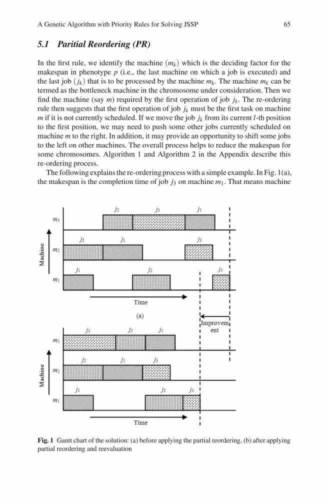
In the first rule, we identify the machine (mk) which is the deciding factor for themakespan in phenotype p (i.e., the last machine on which a job is executed) andthe last job ( jk) that is to be processed by the machine mk. The machine mk can betermed as the bottleneck machine in the chromosome under consideration. Then wefind the machine (say m) required by the first operation of job jk. The re-orderingrule then suggests that the first operation of job jk must be the first task on machinem if it is not currently scheduled. If we move the job jk from its current l-th positionto the first position, we may need to push some other jobs currently scheduled onmachine m to the right. In addition, it may provide an opportunity to shift some jobsto the left on other machines. The overall process helps to reduce the makespan forsome chromosomes. Algorithm 1 and Algorithm 2 in the Appendix describe thisre-ordering process.

The following explains the re-ordering process with a simple example. In Fig. 1(a),the makespan is the completion time of job j3 on machine m1. That means machine

Fig. 1 Gantt chart of the solution: (a) before applying the partial reordering, (b) after applyingpartial reordering and reevaluation


m1 is the bottleneck machine. Here, job j3 requires machine m3 for its first opera-tion. If we move j3 from its current position to the first operation of machine m3,it is necessary to shift job j2 to the right for a feasible schedule on machine m3.These changes create an opportunity for the jobs j1 on m3, j3 on m2 and j3 on m1

to be shifted towards the left without violating the operational sequences. As can beseen in Fig. 1(b), the resulting chromosome is able to improve its makespan. Thechange of makespan is indicated by the dotted lines. Algorithm 2 in the Appendixalso shows how the partial reordering can be done.

5.2 Gap Reduction (GR)

After each generation, the generated phenotype usually leaves some gaps betweenthe jobs. Sometimes, these gaps are necessary to satisfy the precedence constraints.

Fig. 2 Two steps of a partial Gantt chart while building the schedule from the phenotype fora 3×3 job-shop scheduling problem. The X axis represents the execution time and the Y axisrepresents the machines.


However, in some cases, a gap could be removed or reduced by replacing the gapwith a job on the right side of the gap. For a given machine, this is like swappingbetween a gap from the left and a job from the right of a schedule. In addition, agap may be removed or reduced by simply moving a job on the right-hand side ofthe gap leftwards. This process would help developing a compact schedule from theleft and continuing up to the last job for each machine. Of course, it must ensure noconflict or no infeasibility before accepting the move.

Thus, the rule must identify the gaps in each machine, and the candidate jobswhich can be placed in those gaps, without violating the constraints and withoutincreasing the makespan. The same process is carried out for any possible leftwardsshift of jobs of the schedule.

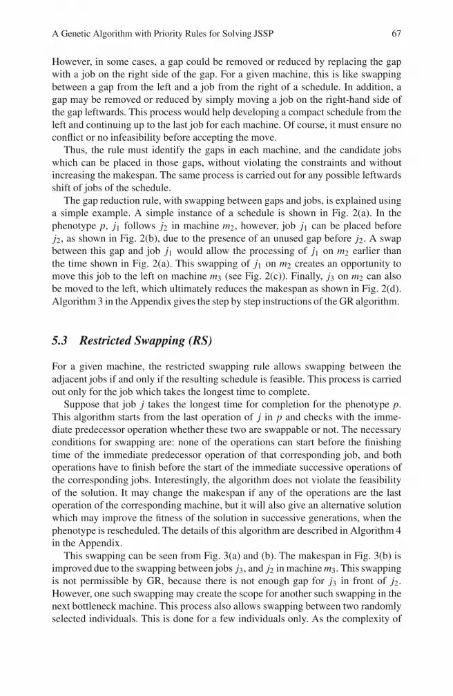
The gap reduction rule, with swapping between gaps and jobs, is explained usinga simple example. A simple instance of a schedule is shown in Fig. 2(a). In thephenotype p, j1 follows j2 in machine m2, however, job j1 can be placed beforej2, as shown in Fig. 2(b), due to the presence of an unused gap before j2. A swapbetween this gap and job j1 would allow the processing of j1 on m2 earlier thanthe time shown in Fig. 2(a). This swapping of j1 on m2 creates an opportunity tomove this job to the left on machine m3 (see Fig. 2(c)). Finally, j3 on m2 can alsobe moved to the left, which ultimately reduces the makespan as shown in Fig. 2(d).Algorithm 3 in the Appendix gives the step by step instructions of the GR algorithm.

5.3 Restricted Swapping (RS)

For a given machine, the restricted swapping rule allows swapping between theadjacent jobs if and only if the resulting schedule is feasible. This process is carriedout only for the job which takes the longest time to complete.

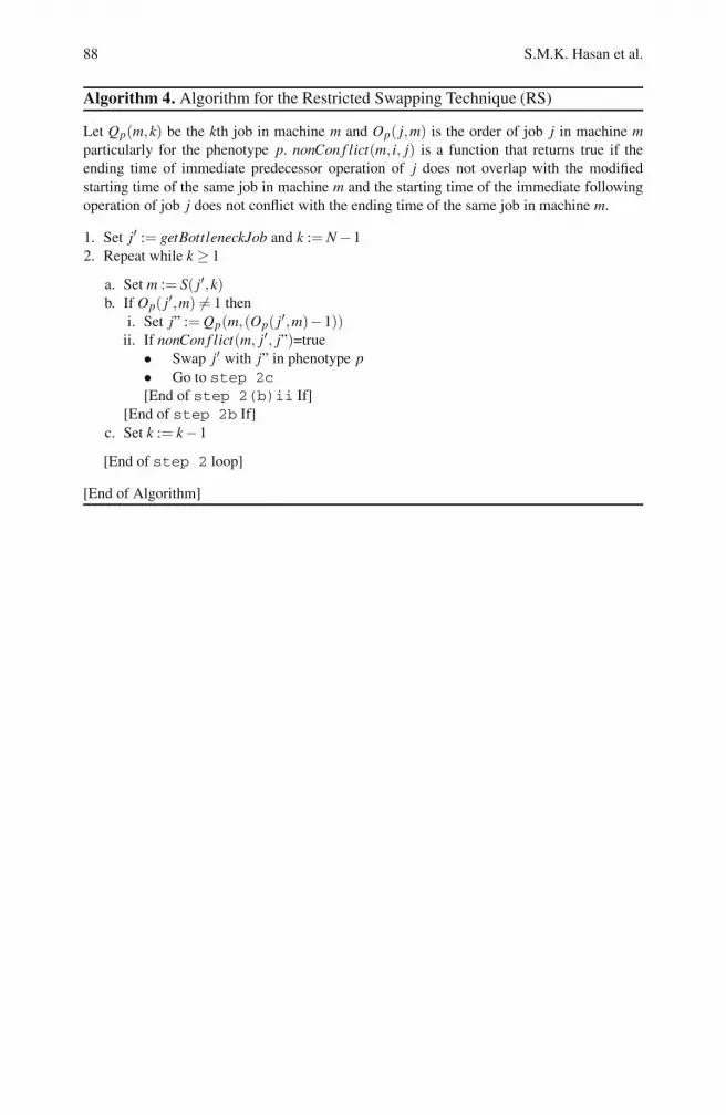
Suppose that job j takes the longest time for completion for the phenotype p.This algorithm starts from the last operation of j in p and checks with the imme-diate predecessor operation whether these two are swappable or not. The necessaryconditions for swapping are: none of the operations can start before the finishingtime of the immediate predecessor operation of that corresponding job, and bothoperations have to finish before the start of the immediate successive operations ofthe corresponding jobs. Interestingly, the algorithm does not violate the feasibilityof the solution. It may change the makespan if any of the operations are the lastoperation of the corresponding machine, but it will also give an alternative solutionwhich may improve the fitness of the solution in successive generations, when thephenotype is rescheduled. The details of this algorithm are described in Algorithm 4in the Appendix.

This swapping can be seen from Fig. 3(a) and (b). The makespan in Fig. 3(b) isimproved due to the swapping between jobs j3, and j2 in machine m3. This swappingis not permissible by GR, because there is not enough gap for j3 in front of j2.However, one such swapping may create the scope for another such swapping in thenext bottleneck machine. This process also allows swapping between two randomlyselected individuals. This is done for a few individuals only. As the complexity of


Fig. 3 Gantt chart of the solution: (a) before applying the restricted swapping, (b) after ap-plying restricted swapping and reevaluation.

this algorithm is simply of order N, it does not affect the overall computationalcomplexity much.

6 Implementation

For the initial implementation of TGA, we generate a set of random individuals.Each individual is represented by a binary chromosome. We use the job-pair rela-tionship based representation as Nakano and Yamada [37] and Paredis et al. [40]successfully used this representation to solve job-shop scheduling problems and re-ported the effectiveness of the representation. We use the simple two-point crossoverand bit flip mutation as reproduction operators. We have carried out a set of exper-iments with different crossover and mutation rates to analyze the robustness of the


algorithm. After the successful implementation of the TGA, we introduce the prior-ity rules, as discussed in the last section, to TGA as follows:

• Partial re-ordering rule with TGA (PR-GA)• Gap reduction rule with TGA (GR-GA) and• Gap reduction and restricted swapping rule with TGA (GR-RS-GA)

For ease of explanation, we describe the steps of GR-RS-GA below:

Let Rc and Rm be the selection probabilities for two-point crossover and bit-flip mutation respectively. P′(t) is the set of current individuals at time t andP(t) is the evaluated set of individuals which is the set of individuals repairedusing local and global harmonization at time t. K is the total number of indi-viduals in each generation. s is an index which indicates a particular individualin the current population.

1. Initialize P′(t) as a random population P′(t = 0) of size K, where eachrandom individual is a bit string of length l.

2. Repeat until some stopping criteria are meta. Set t := t + 1 and s :=NULLb. Evaluate P(t) from P′(t −1) by the following steps;

i. Decode each individual p by using the job-based decoding withthe local harmonization and global harmonization methods to repairillegal bit strings.

ii. Generate the complete schedule with the starting and ending timeof each operation by applying the gap reduction rule (GR) and cal-culate the objective function f of p.

iii. Go to step 2(b)i until every individual is evaluated.iv. Rank the individuals according to the fitness values from higher to

lower fitness value.v. Apply elitism; i.e., preserve the solution having the best fitness

value in the current generation so that it can survive at least untilto the next generation.

c. Apply the restricted swapping rule (RS) on some of the individuals se-lected in a random manner.

d. Go to step 3 if the stopping criteria are met.e. Modify P(t) using the following steps;

i. Select the current individual p from P(t) and select a random num-ber R between 0 and 1.

ii. If R Rc thenA. If s =NULL

• Save the location of p into s.• Go to step 2(e)i.[End of step 2(e)iiA If]


B. Select randomly one individual p1 from the top 15% of the pop-ulation and two individuals from the rest. Play a tournament be-tween the last two and choose the winning individual w. Applytwo-point crossover between p1 and w; generate p1 and w. Re-place p with p1 and content of s with w. Set s with NULL.

C. Else if R > Rc and R (Rc + Rm) then randomly select one indi-vidual p1 from P(t) and apply bit-flip mutation. Replace p withp1.

D. Else continue.[End of step 2(e)ii If]

iii. Reassign the P′(t) by P(t) to initialize the new generation preserv-ing the best solution as elite.

[End of step 2a Loop]3. Save the best solution among all the feasible solutions.

[End of Algorithm]

Sometimes the actions of the genetic operators may direct the good individualsto less attractive regions in the search space. In this case, the elitism would ensurethe survival of the best individuals [26, 27]. We apply elitism in each generation topreserve the best solution found so far and also to inherit the elite individuals moreoften than the rest.

During the crossover operation, we use the tournament selection that chooses oneindividual from the elite class of individuals (i.e., the top 15%) and two individualsfrom the rest. Increasing that rate reduces the quality of solutions. On the otherhand, reducing the rate initiates a quicker but premature convergence. This selectionthen plays a tournament between the last two and performs crossover between thewinner and the elite individual. As we apply a single selection process for boththe reproduction processes, the probability of selecting an individual multiple timesis low, but not zero. We rank the individuals on the basis of their fitness values,and a high selection pressure on the better individuals may contribute to prematureconvergence. Consequently, we consider the situation where 50% or more of theelite class are the same solution. In this case, their offspring will be quite similarafter some generations. To counter this, when this occurs, a higher mutation ratewill be used to help diversify the population. We set the population size to 2500 andthe number of generations to 1000. In our approach, the GR rule is used as a partof evaluation. That means GR is applied to every individual. On the other hand, weapply PR and RS to only 5% of randomly selected individuals in every generation.Because of the role of GR in the evaluation process, it is not possible to applyit as an additional component like PR or RS. Moreover, PR and RS are effectiveon feasible individuals which prohibit using these rules before evaluation. To testthe performance of our proposed algorithms, we have solved the 40 benchmarkproblems designed by Lawrence [34] and have compared our results with severalexisting algorithms. The problems range from 10×5 to 30×10 and 15×15 whereN ×M represents N jobs and M machines.


7 Result and Analysis

The results for the benchmark problems were obtained by executing the algorithmson a personal computer. All results are based on 30 independent runs with differ-ent random seeds. To select the appropriate set of parameters, we have performedseveral experiments varying the reproduction parameters (crossover and mutation).The results presented below are based on the best parameter set. The details of para-metric analysis are discussed later in the chapter. These results and parameters aretabulated in Table 2-Table 7.

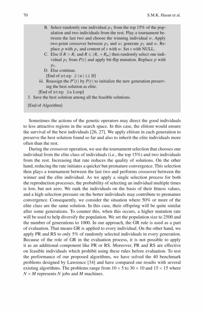
Table 2 Comparing our Four Algorithms

No. ofProblems

AlgorithmOptimalFound

ARD(%)

SDRD(%)

Fitness Eval.(103)

40(la01-la40)

TGA 15 3.591 4.165 664.90PR-GA 16 3.503 4.192 660.86GR-GA 23 1.360 2.250 356.41GR-RS-GA 27 0.968 1.656 388.58

Table 2 compares the performance of our four algorithms (TGA, PR-GA, GR-GA, and GR-RS-GA) in terms of the percentage average relative deviation (ARD)from the best result published in literature, the standard deviation of the percentagerelative deviation (SDRD), and the total number of evaluations required. We do notconsider the CPU time as a unit of measurement due to the fact that we have con-ducted our experiments using different platforms and the unavailability of such in-formation in the literature. From Table 2, it is clear that the performance of GR-GAis better than both PR-GA and TGA. The addition of RS to GR-GA, which is knownas GR-RS-GA, has clearly enhanced the performance of the algorithm. Out of the 40test problems, both GR-GA and GR-RS-GA obtained exact optimal solutions for 23problems. In addition, GR-RS-GA obtained optimal solutions for 4 more problemsand substantially improved solutions for 10 problems. In general, these two algo-rithms converge quickly as can be seen from the average number of generations.

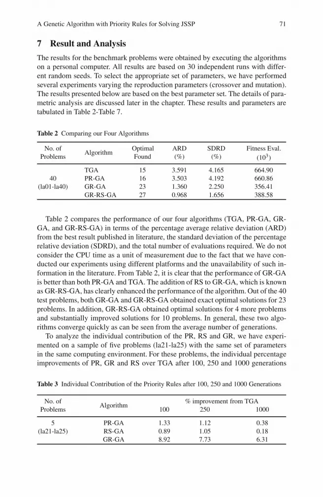
To analyze the individual contribution of the PR, RS and GR, we have experi-mented on a sample of five problems (la21-la25) with the same set of parametersin the same computing environment. For these problems, the individual percentageimprovements of PR, GR and RS over TGA after 100, 250 and 1000 generations

Table 3 Individual Contribution of the Priority Rules after 100, 250 and 1000 Generations

No. ofProblems

Algorithm% improvement from TGA

100 250 1000

5(la21-la25)

PR-GA 1.33 1.12 0.38RS-GA 0.89 1.05 0.18GR-GA 8.92 7.73 6.31


are reported in Table 3. To measure this, we calculate the improvement of the g-thgeneration from the (g−1)-th generation up to the G-th generation where G is 100,250 and 1000 respectively.

The result in Table 3 is the average of the improvements in percentage scale.Although all three priority rules have a positive effect, GR’s contribution is signifi-cantly higher than the other two rules and is consistent over many generations.

Interestingly, the improvement rapidly decreases in the case of GR comparedto PR and RS. The reason for this is that, GR-GA starts with a set of good initialsolutions, for example, an 18.17% improvement compared to TGA for the problemsla21-la25. This is why, the effects in each generation decrease simultaneously.

To observe the contribution more closely, we measure the improvement due to theindividual rule in every generation in the first 100 generations. A sample comparisonof the fitness values for our three algorithms in the first 100 generations is shown inFig. 4. It is clear from the figures that the improvement rates of TGA, PR-GA andRS-GA are higher than GR-GA, but GR-GA provides better fitness in all the testedproblems. As JSSP is a minimization problem, GR-GA outperforms the others everycase.

PR considers only the bottleneck job, whereas GR is applied to all individuals.The process of GR eventually makes most of the changes performed by PR oversome (or many) generations. We identify a number of individuals where PR couldmake a positive contribution. We apply GR and PR on those individuals, to comparetheir relative contribution. For the five problems we consider over 1000 generations,we observe that GR made a 9.13% more improvement than PR. It must be notedhere that GR is able to make all the changes which PR does. That means PR cannotmake an extra contribution over GR. As a result, the inclusion of PR with GR doesnot help to improve the performance of the algorithm. That is why we do not presentother possible variants, such as PR-RS-GA and GR-RS-PR-GA.

Both PR and RS were applied only to 5% of the individuals. The role of RSis mainly to increase the diversity. A higher rate of PR and RS does not providesignificant benefit either in terms of quality of solution or computational time. Wehave experimented with varying the rate of PR and RS individually from 5% to25% and tabulated the percentage relative improvement from TGA in Table 4. FromTable 4, it is clear that the increase of the rate of applying PR and RS does notimprove the quality of the solutions. Moreover, it was found from experiments thatit takes extra time to converge.

Table 5 presents the percentage of relative deviation from the best known solu-tion, for 40 test problems, for our four algorithms. Table 6 shows the same resultsfor a number of well-known algorithms appearing in the literature. The first twocolumns of Table 5 represent the problem instances and the size of the problems.These columns are followed by the average relative deviation (ARD) of the best fit-ness found from four of our algorithms compared to the best fitness found from theliterature in percentage scale.


(a)

(b)

(c)

Fig. 4 Fitness curve for the problem la21–la25 up to the first 100 generations


(d)

(e)

Fig. 4 (continued)

Table 6 starts with the column of problem instance and each column next to thatrepresents the ARD in percentage of some other algorithms found in the literature.Here, we consider our four algorithms (TGA, PR-GA, GR-GA, and GR-RS-GA),local search GA [27, 38], GA with genetic programming [48], GRASP [8], normalGA and shifting-bottleneck GA [18], local search GA [1], GA [16] and shiftingbottleneck heuristic [2]. The details of these algorithms were discussed in earliersections of this chapter.

As shown in Table 5 and Table 6, for most of the test problems, our proposed GR-RS-GA performs better than other algorithms in terms of the quality of solutions.To compare the overall performance of these algorithms, we calculate the averageof relative deviation (ARD) for the test problems and the standard deviation of therelative deviations (SDRD), and present them in Table 7. In Table 7, we compare theoverall performance with only our GR-RS-GA. As different authors used different


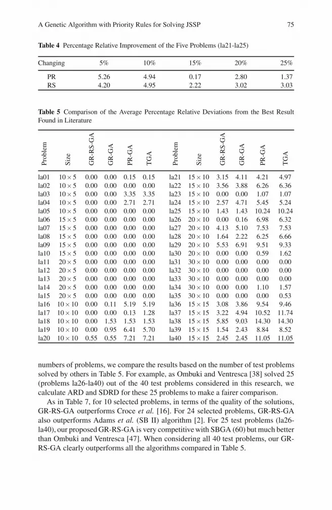
Table 4 Percentage Relative Improvement of the Five Problems (la21-la25)

Changing 5% 10% 15% 20% 25%

PR 5.26 4.94 0.17 2.80 1.37RS 4.20 4.95 2.22 3.02 3.03

Table 5 Comparison of the Average Percentage Relative Deviations from the Best ResultFound in Literature

Pro

blem

Siz

e

GR

-RS

-GA

GR

-GA

PR

-GA

TG

A

Pro

blem

Siz

e

GR

-RS

-GA

GR

-GA

PR

-GA

TG

A

la01 10×5 0.00 0.00 0.15 0.15 la21 15×10 3.15 4.11 4.21 4.97la02 10×5 0.00 0.00 0.00 0.00 la22 15×10 3.56 3.88 6.26 6.36la03 10×5 0.00 0.00 3.35 3.35 la23 15×10 0.00 0.00 1.07 1.07la04 10×5 0.00 0.00 2.71 2.71 la24 15×10 2.57 4.71 5.45 5.24la05 10×5 0.00 0.00 0.00 0.00 la25 15×10 1.43 1.43 10.24 10.24la06 15×5 0.00 0.00 0.00 0.00 la26 20×10 0.00 0.16 6.98 6.32la07 15×5 0.00 0.00 0.00 0.00 la27 20×10 4.13 5.10 7.53 7.53la08 15×5 0.00 0.00 0.00 0.00 la28 20×10 1.64 2.22 6.25 6.66la09 15×5 0.00 0.00 0.00 0.00 la29 20×10 5.53 6.91 9.51 9.33la10 15×5 0.00 0.00 0.00 0.00 la30 20×10 0.00 0.00 0.59 1.62la11 20×5 0.00 0.00 0.00 0.00 la31 30×10 0.00 0.00 0.00 0.00la12 20×5 0.00 0.00 0.00 0.00 la32 30×10 0.00 0.00 0.00 0.00la13 20×5 0.00 0.00 0.00 0.00 la33 30×10 0.00 0.00 0.00 0.00la14 20×5 0.00 0.00 0.00 0.00 la34 30×10 0.00 0.00 1.10 1.57la15 20×5 0.00 0.00 0.00 0.00 la35 30×10 0.00 0.00 0.00 0.53la16 10×10 0.00 0.11 5.19 5.19 la36 15×15 3.08 3.86 9.54 9.46la17 10×10 0.00 0.00 0.13 1.28 la37 15×15 3.22 4.94 10.52 11.74la18 10×10 0.00 1.53 1.53 1.53 la38 15×15 5.85 9.03 14.30 14.30la19 10×10 0.00 0.95 6.41 5.70 la39 15×15 1.54 2.43 8.84 8.52la20 10×10 0.55 0.55 7.21 7.21 la40 15×15 2.45 2.45 11.05 11.05

numbers of problems, we compare the results based on the number of test problemssolved by others in Table 5. For example, as Ombuki and Ventresca [38] solved 25(problems la26-la40) out of the 40 test problems considered in this research, wecalculate ARD and SDRD for these 25 problems to make a fairer comparison.

As in Table 7, for 10 selected problems, in terms of the quality of the solutions,GR-RS-GA outperforms Croce et al. [16]. For 24 selected problems, GR-RS-GAalso outperforms Adams et al. (SB II) algorithm [2]. For 25 test problems (la26-la40), our proposed GR-RS-GA is very competitive with SBGA (60) but much betterthan Ombuki and Ventresca [47]. When considering all 40 test problems, our GR-RS-GA clearly outperforms all the algorithms compared in Table 5.


Table 6 Comparison of the Percentage Relative Deviations from the Best Results with thatof Other Authors

Prob

lem

Gon

calv

eset

al.

Wer

ner

etal

.

Aarts et al.

Om

buki

&V

entr

esca Dorndorf & Pesch

Cro

ceet

al.

Bin

ato

etal

.

Adams et al.

GL

S1

GL

S2

PGA

SBG

A-1

SBG

A-2

SB-I

SB-I

I

la01 0.00 0.00 0.00 0.00 0.00 0.00 0.00 0.00la02 1.50 1.98 0.61 3.97 1.68 1.68 0.00 9.92 2.14la03 1.16 2.68 2.01 3.85 1.17 11.56 1.17 4.36 1.34la04 0.00 1.53 0.68 5.08 0.00 0.00 1.19 0.51la05 0.00 0.00 0.00 0.00 0.00 0.00 0.00la06 0.00 0.00 0.00 0.00 0.00 0.00 0.00 0.00la07 0.00 0.00 0.00 0.00 0.00 0.00 0.00la08 0.00 0.00 0.00 0.00 0.00 0.00 0.58 0.00la09 0.00 0.00 0.00 0.00 0.00 0.00 0.00la10 0.00 0.00 0.00 0.00 0.00 0.00 0.10la11 0.00 0.00 0.00 0.00 0.00 0.00 0.00 0.00la12 0.00 0.00 0.00 0.00 0.00 0.00 0.00la13 0.00 0.00 0.00 0.00 0.00 0.00 0.00la14 0.00 0.00 0.00 0.00 0.00 0.00 0.00la15 0.00 0.00 0.00 2.49 0.00 0.00 0.00la16 2.88 3.60 3.39 3.39 1.48 6.67 1.69 1.69 3.60 0.11 8.04 3.49la17 1.01 2.42 0.89 0.89 1.02 3.19 0.38 0.00 0.00 1.53 0.38la18 0.82 3.42 0.94 1.18 1.06 8.02 0.00 0.00 0.00 5.07 1.30la19 1.06 4.87 2.49 2.02 2.14 4.51 2.49 0.71 0.00 3.92 2.14la20 2.59 4.10 1.22 1.55 0.55 2.88 1.00 0.89 0.55 2.44 1.33la21 3.06 14.53 3.63 3.73 6.50 8.89 2.68 2.68 4.88 4.30 12.05 3.63la22 2.42 2.91 1.83 6.69 7.66 0.86 0.97 3.56 12.19 1.83la23 0.00 0.00 0.00 0.29 3.88 0.00 0.00 0.00 2.81 0.00la24 3.61 11.23 3.74 4.92 10.37 8.45 2.67 2.35 4.60 6.95 4.39la25 3.55 12.59 3.99 3.38 7.16 3.79 3.17 3.07 5.22 7.27 4.09la26 0.00 1.81 1.48 7.31 4.93 0.08 0.00 1.07 4.35 7.06 0.49la27 3.67 17.00 5.91 5.26 9.31 11.58 3.00 2.75 6.88 7.29 4.53la28 2.72 5.35 4.03 7.89 9.13 1.97 2.06 6.33 3.29 2.80la29 4.06 20.22 11.50 8.90 13.31 15.47 4.06 4.58 11.75 11.84 7.09la30 0.00 3.47 2.29 7.08 4.13 0.00 0.00 0.96 3.54 0.00la31 0.00 0.00 0.00 0.00 0.00 0.00 0.00 0.00 0.00 0.00la32 0.00 0.00 0.00 0.00 0.00 0.00 0.00 0.00 0.00la33 0.00 0.00 0.00 1.51 0.00 0.00 0.00 0.00 0.00la34 0.00 0.93 0.52 3.66 0.00 0.00 0.00 1.86 0.00la35 0.00 0.32 0.11 3.71 0.00 0.00 0.00 0.00 0.00la36 2.69 4.42 3.39 7.10 8.28 3.86 3.86 2.92 5.21 6.55 2.92la37 2.78 3.72 3.79 8.59 7.23 6.23 3.51 4.29 6.30 1.86la38 4.47 17.64 7.44 7.27 13.88 8.36 4.60 3.76 5.94 7.02 4.93la39 1.36 3.73 3.73 12.81 9.57 3.97 3.57 4.62 7.14 3.24la40 2.40 20.54 4.17 3.11 8.27 8.10 4.26 2.45 3.03 8.51 3.85


Table 7 Comparing the Algorithms Based on Average Relative Deviations and Standard De-viation of Average Relative Deviations

No. of Problems Test Problems Author Algorithm ARD(%) SDRD(%)

40la01la40

Our Proposed GR-RS-GA 0.97 1.66Gonalves et al. Non-delay 1.20 1.48Aarts et al. GLS1 4.00 4.09Aarts et al. GLS2 2.05 2.53Dorndorf & Pesche PGA 1.75 2.20Dorndorf & Pesche SBGA (40) 1.25 1.72Binato et al. - 1.87 2.78Adams et al. SB I 3.67 3.98

25la16la40

Our Proposed GR-RS-GA 1.55 1.88Ombuki and Ventresca - 5.67 4.38Dorndorf & Pesch SBGA (60) 1.56 1.58

24Selected Our Proposed GR-RS-GA 1.68 1.86

(see Table 6) Adams et al. SB II 2.43 1.85


(see Table 6) Werner et al. GC 11.01 7.02


(see Table 6) Croce et al. - 2.57 3.60

To get a clear view of the performance of our three algorithms over the traditionalGA, we perform a statistical significance test for each of these algorithms againstthe traditional GA. We use the student’s t-test [45] where the t-values are calculatedfrom the average and standard deviation of 30 independent runs for each problem.The values are normally distributed. The results of the test are tabulated in Table 8.

We derive nine levels of significance, to judge the performance of PR-GA, GR-GA, and GR-RS-GA over the TGA, using the critical t-values 1.311 (which is for80% confidence level), 2.045 (for 95% confidence level), and 2.756 (for 99% confi-dence level). We define the significance level S as follows.

S =

⎧⎪⎪⎪⎪⎪⎪⎪⎪⎪⎪⎪⎪⎪⎪⎪⎨⎪⎪⎪⎪⎪⎪⎪⎪⎪⎪⎪⎪⎪⎪⎪⎩

++++ ti ≥ 2.756

+++ 2.045 ≤ ti < 2.756

++ 1.311 ≤ ti < 2.045

+ 0 < ti < 1.311

= ti = 0

− −1.311 < ti < 0

−− −2.045 < ti ≤−1.311

−−− −2.756 < ti ≤−2.045

−−−− ti ≤−2.756

(3)


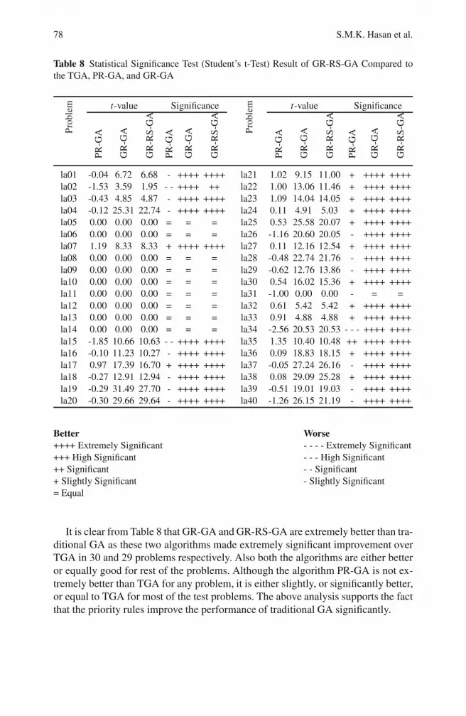
Table 8 Statistical Significance Test (Student’s t-Test) Result of GR-RS-GA Compared tothe TGA, PR-GA, and GR-GA

Pro

blem t-value Significance

Pro

blem t-value Significance

PR

-GA

GR

-GA

GR

-RS

-GA

PR

-GA

GR

-GA

GR

-RS

-GA

PR

-GA

GR

-GA

GR

-RS

-GA

PR

-GA

GR

-GA

GR

-RS

-GA

la01 -0.04 6.72 6.68 - ++++ ++++ la21 1.02 9.15 11.00 + ++++ ++++la02 -1.53 3.59 1.95 - - ++++ ++ la22 1.00 13.06 11.46 + ++++ ++++la03 -0.43 4.85 4.87 - ++++ ++++ la23 1.09 14.04 14.05 + ++++ ++++la04 -0.12 25.31 22.74 - ++++ ++++ la24 0.11 4.91 5.03 + ++++ ++++la05 0.00 0.00 0.00 = = = la25 0.53 25.58 20.07 + ++++ ++++la06 0.00 0.00 0.00 = = = la26 -1.16 20.60 20.05 - ++++ ++++la07 1.19 8.33 8.33 + ++++ ++++ la27 0.11 12.16 12.54 + ++++ ++++la08 0.00 0.00 0.00 = = = la28 -0.48 22.74 21.76 - ++++ ++++la09 0.00 0.00 0.00 = = = la29 -0.62 12.76 13.86 - ++++ ++++la10 0.00 0.00 0.00 = = = la30 0.54 16.02 15.36 + ++++ ++++la11 0.00 0.00 0.00 = = = la31 -1.00 0.00 0.00 - = =la12 0.00 0.00 0.00 = = = la32 0.61 5.42 5.42 + ++++ ++++la13 0.00 0.00 0.00 = = = la33 0.91 4.88 4.88 + ++++ ++++la14 0.00 0.00 0.00 = = = la34 -2.56 20.53 20.53 - - - ++++ ++++la15 -1.85 10.66 10.63 - - ++++ ++++ la35 1.35 10.40 10.48 ++ ++++ ++++la16 -0.10 11.23 10.27 - ++++ ++++ la36 0.09 18.83 18.15 + ++++ ++++la17 0.97 17.39 16.70 + ++++ ++++ la37 -0.05 27.24 26.16 - ++++ ++++la18 -0.27 12.91 12.94 - ++++ ++++ la38 0.08 29.09 25.28 + ++++ ++++la19 -0.29 31.49 27.70 - ++++ ++++ la39 -0.51 19.01 19.03 - ++++ ++++la20 -0.30 29.66 29.64 - ++++ ++++ la40 -1.26 26.15 21.19 - ++++ ++++

Better Worse++++ Extremely Significant - - - - Extremely Significant+++ High Significant - - - High Significant++ Significant - - Significant+ Slightly Significant - Slightly Significant= Equal

It is clear from Table 8 that GR-GA and GR-RS-GA are extremely better than tra-ditional GA as these two algorithms made extremely significant improvement overTGA in 30 and 29 problems respectively. Also both the algorithms are either betteror equally good for rest of the problems. Although the algorithm PR-GA is not ex-tremely better than TGA for any problem, it is either slightly, or significantly better,or equal to TGA for most of the test problems. The above analysis supports the factthat the priority rules improve the performance of traditional GA significantly.


7.1 Parameter Analysis

In GA, different reproduction parameters are used. We have performed experimentswith different combinations of parameters to identify the appropriate set of param-eters and their effect on solutions. A higher selection pressure on better individuals,with a higher rate of crossover, contributes towards diversity reduction and hencethe solutions converge prematurely. In JSSPs, when a large portion of the populationconverges to particular solutions, the probability of solution improvement reducesbecause the rate of selecting the same solution increases. Therefore, it is importantto find an appropriate rate for crossover and mutation. Three sets of experimentswere carried out as follows:

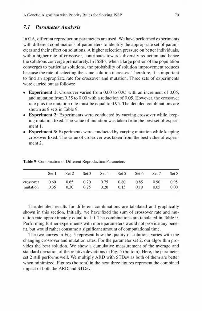
• Experiment 1: Crossover varied from 0.60 to 0.95 with an increment of 0.05,and mutation from 0.35 to 0.00 with a reduction of 0.05. However, the crossoverrate plus the mutation rate must be equal to 0.95. The detailed combinations areshown as 8 sets in Table 9.

• Experiment 2: Experiments were conducted by varying crossover while keep-ing mutation fixed. The value of mutation was taken from the best set of experi-ment 1.

• Experiment 3: Experiments were conducted by varying mutation while keepingcrossover fixed. The value of crossover was taken from the best value of experi-ment 2.

Table 9 Combination of Different Reproduction Parameters

Set 1 Set 2 Set 3 Set 4 Set 5 Set 6 Set 7 Set 8

crossover 0.60 0.65 0.70 0.75 0.80 0.85 0.90 0.95mutation 0.35 0.30 0.25 0.20 0.15 0.10 0.05 0.00

The detailed results for different combinations are tabulated and graphicallyshown in this section. Initially, we have fixed the sum of crossover rate and mu-tation rate approximately equal to 1.0. The combinations are tabulated in Table 9.Performing further experiments with more parameters would not provide any bene-fit, but would rather consume a significant amount of computational time.

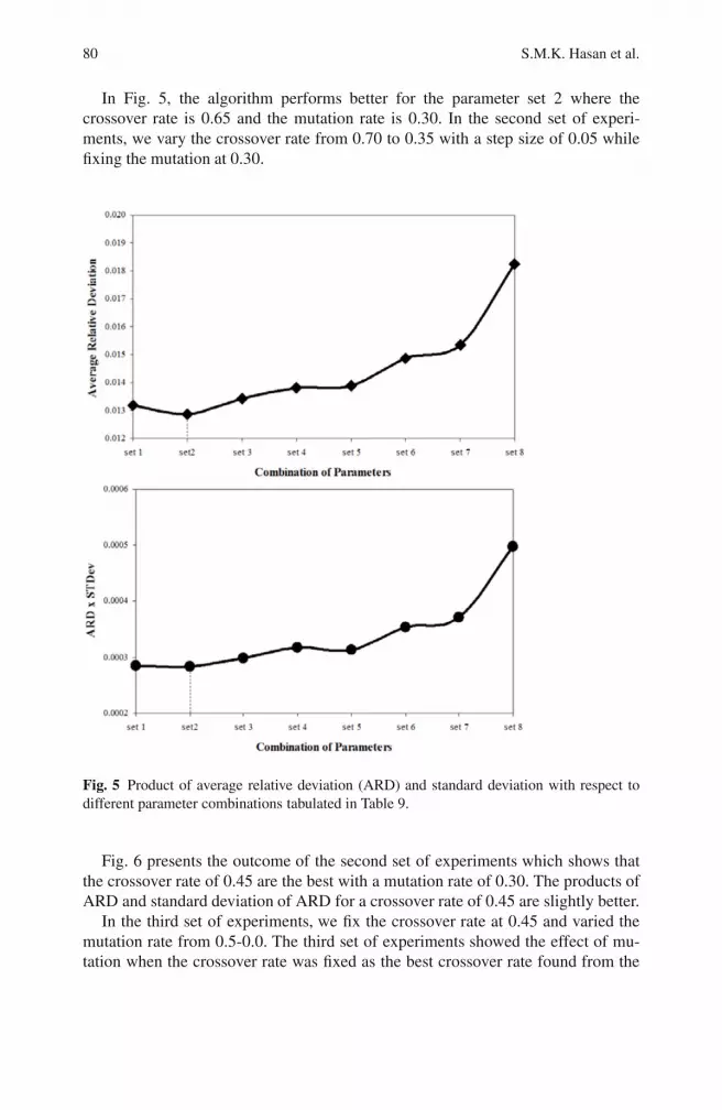
The two curves in Fig. 5 represent how the quality of solutions varies with thechanging crossover and mutation rates. For the parameter set 2, our algorithm pro-vides the best solution. We show a cumulative measurement of the average andstandard deviation of the relative deviations in Fig. 5 (bottom). Here, the parameterset 2 still performs well. We multiply ARD with STDev as both of them are betterwhen minimized. Figures (bottom) in the next three figures represent the combinedimpact of both the ARD and STDev.


In Fig. 5, the algorithm performs better for the parameter set 2 where thecrossover rate is 0.65 and the mutation rate is 0.30. In the second set of experi-ments, we vary the crossover rate from 0.70 to 0.35 with a step size of 0.05 whilefixing the mutation at 0.30.

Fig. 5 Product of average relative deviation (ARD) and standard deviation with respect todifferent parameter combinations tabulated in Table 9.

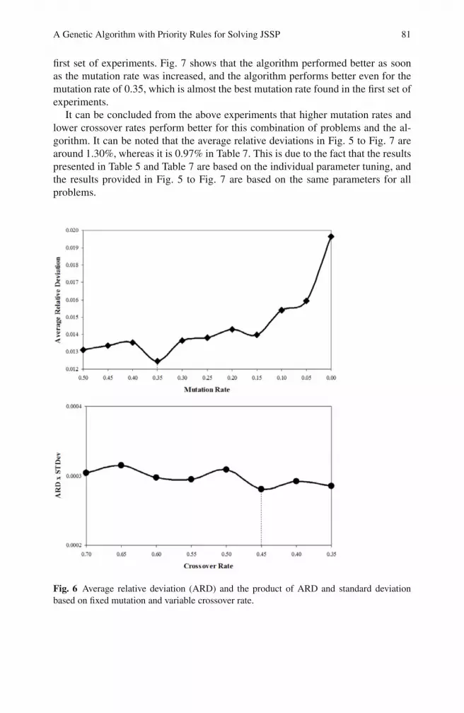
Fig. 6 presents the outcome of the second set of experiments which shows thatthe crossover rate of 0.45 are the best with a mutation rate of 0.30. The products ofARD and standard deviation of ARD for a crossover rate of 0.45 are slightly better.

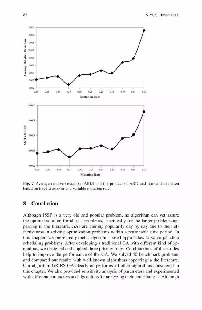
In the third set of experiments, we fix the crossover rate at 0.45 and varied themutation rate from 0.5-0.0. The third set of experiments showed the effect of mu-tation when the crossover rate was fixed as the best crossover rate found from the


first set of experiments. Fig. 7 shows that the algorithm performed better as soonas the mutation rate was increased, and the algorithm performs better even for themutation rate of 0.35, which is almost the best mutation rate found in the first set ofexperiments.

It can be concluded from the above experiments that higher mutation rates andlower crossover rates perform better for this combination of problems and the al-gorithm. It can be noted that the average relative deviations in Fig. 5 to Fig. 7 arearound 1.30%, whereas it is 0.97% in Table 7. This is due to the fact that the resultspresented in Table 5 and Table 7 are based on the individual parameter tuning, andthe results provided in Fig. 5 to Fig. 7 are based on the same parameters for allproblems.

Fig. 6 Average relative deviation (ARD) and the product of ARD and standard deviationbased on fixed mutation and variable crossover rate.


Fig. 7 Average relative deviation (ARD) and the product of ARD and standard deviationbased on fixed crossover and variable mutation rate.

8 Conclusion

Although JSSP is a very old and popular problem, no algorithm can yet assurethe optimal solution for all test problems, specifically for the larger problems ap-pearing in the literature. GAs are gaining popularity day by day due to their ef-fectiveness in solving optimization problems within a reasonable time period. Inthis chapter, we presented genetic algorithm based approaches to solve job-shopscheduling problems. After developing a traditional GA with different kind of op-erations, we designed and applied three priority rules. Combinations of these ruleshelp to improve the performance of the GA. We solved 40 benchmark problemsand compared our results with well-known algorithms appearing in the literature.Our algorithm GR-RS-GA clearly outperforms all other algorithms considered inthis chapter. We also provided sensitivity analysis of parameters and experimentedwith different parameters and algorithms for analyzing their contributions. Although


our algorithm performed well, we feel that the algorithm requires further work toensure consistent performance for a wide range of practical JSSPs. We have exper-imented with different sizes of the test problems varying from 10× 5 to 30× 10.To justify the robustness of the algorithms, we would like to conduct experimentson large-scale problems with higher complexities. The real life job-shop schedulingproblems may not be as straight forward as we considered here. The problems mayinvolve different kinds of uncertainties and constraints. Therefore, we would alsolike to extend our research by introducing situations like machine breakdown, dy-namic job arrival, machine addition and removal, due date restrictions and others.For the case of machine breakdown, we would like to consider two different sce-narios: (i) the breakdown information is known in advance, and (ii) the breakdownhappened while the schedule is on process. The later case is more practical in termsof the real-life problems. Regarding the dynamic job arrival, our objective is to re-optimize the remaining operations along with the newly arrived job as a separatesub-problem. Machine addition and removal require reorganizing the operations re-lated to the new/affected machine(s). Changing the due date might be similar tochanging the priority of an existing job. Setting the preferred due dates may relaxor tighten the remaining operations after re-optimization. Finally, the proposed al-gorithms are significant contributions to the research into solving JSSPs.

References

1. Aarts, E.H.L., Van Laarhoven, P.J.M., Lenstra, J.K., Ulder, N.L.J.: A computational studyof local search algorithms for job shop scheduling. ORSA Journal on Computing 6(2),118–125 (1994)

2. Adams, J., Balas, E., Zawack, D.: The shifting bottleneck procedure for job shop schedul-ing. Management Science 34(3), 391–401 (1988)

3. Akers Jr., S.B., Friedman, J.: A non-numerical approach to production scheduling prob-lems. Journal of the Operations Research Society of America 3(4), 429–442 (1955)

4. Ashour, S., Hiremath, S.R.: A branch-and-bound approach to the job-shop schedulingproblem. International Journal of Production Research 11(1), 47–58 (1973)

5. Baker, K.R.: Introduction to sequencing and scheduling. Wiley, New York (1974)6. Barnes, J.W., Chambers, J.B.: Solving the job shop scheduling problem with tabu search.

IIE Transactions 27(2), 257–263 (1995)7. Biegel, J.E., Davern, J.J.: Genetic algorithms and job shop scheduling. Computers &

Industrial Engineering 19(1-4), 81–91 (1990)8. Binato, S., Hery, W.J., Loewenstern, D.M., Resende, M.G.C.: A grasp for job shop

scheduling. In: Ribeiro, C.C., Hansen, P. (eds.) Essays and surveys on metaheuristics,pp. 58–79. Kluwer Academic Publishers, Boston (2001)

9. Bresina, J.L.: Heuristic-biased stochastic sampling. In: 13th National Conference on Ar-tificial Intelligence, vol. 1, pp. 271–278. CSA Illumina, Portland (1996)

10. Brucker, P., Jurisch, B., Sievers, B.: A branch and bound algorithm for the job-shopscheduling problem. Discrete Applied Mathematics 49(1-3), 107–127 (1994)

11. Carlier, J.: The one-machine sequencing problem. European Journal of Operational Re-search 11(1), 42–47 (1982)


12. Carlier, J., Pinson, E.: An algorithm for solving the job-shop problem. Management Sci-ence 35(2), 164–176 (1989)

13. Cheng, R., Gen, M., Tsujimura, Y.: A tutorial survey of job-shop scheduling problemsusing genetic algorithms–i. representation. Computers & Industrial Engineering 30(4),983–997 (1996)

14. Conway, R.W., Maxwell, W.L., Miller, L.W.: Theory of scheduling. Addison-WesleyPub. Co., Reading (1967)

15. Dauzere-Peres, S., Lasserre, J.B.: A modified shifting bottleneck procedure for job-shopscheduling. International Journal of Production Research 31(4), 923–932 (1993)

16. Della-Croce, F., Tadei, R., Volta, G.: A genetic algorithm for the job shop problem. Com-puters & Operations Research 22(1), 15–24 (1995)

17. Dell’Amico, M., Trubian, M.: Applying tabu search to the job-shop scheduling problem.Annals of Operations Research 41(3), 231–252 (1993)

18. Dorndorf, U., Pesch, E.: Evolution based learning in a job shop scheduling environment.Computers & Operations Research 22(1), 25–40 (1995)

19. Emmons, H.: One-machine sequencing to minimize certain functions of job tardiness.Operations Research 17(4), 701–715 (1969)

20. Feo, T.A., Resende, M.G.C.: A probabilistic heuristic for a computationally difficult setcovering problem. Operations Research Letters 8(2), 67–71 (1989)

21. French, S.: Sequencing and scheduling: an introduction to the mathematics of the job-shop. Ellis Horwood series in mathematics and its applications. E. Horwood; Wiley,Chichester, White Sussex (1982)

22. Garey, M.R., Johnson, D.S.: Computers and intractability: a guide to the theory of NP-completeness. Freeman, W. H., San Francisco (1979)

23. Garey, M.R., Johnson, D.S., Sethi, R.: The complexity of flowshop and jobshop schedul-ing. Mathematics of Operations Research 1(2), 117–129 (1976)

24. Giffler, B., Thompson, G.L.: Algorithms for solving production-scheduling problems.Operations Research 8(4), 487–503 (1960)

25. Glover, F.: Tabu search – part i. ORSA Journal on Computing 1(3), 190 (1989)26. Goldberg, D.E.: Genetic algorithms in search, optimization, and machine learning.

Addison-Wesley Pub. Co., Reading (1989)27. Goncalves, J.F., de Magalhaes, M., Jorge, J., Resende, M.G.C.: A hybrid genetic al-

gorithm for the job shop scheduling problem. European Journal of Operational Re-search 167(1), 77–95 (2005)

28. Hasan, S.M.K., Sarker, R., Cornforth, D.: Hybrid genetic algorithm for solving job-shopscheduling problem. In: 6th IEEE/ACIS International Conference on Computer and In-formation Science, pp. 519–524. IEEE Computer Society Press, Melbourne (2007)

29. Hasan, S.M.K., Sarker, R., Cornforth, D.: Modified genetic algorithm for job-shopscheduling: A gap-utilization technique. In: IEEE Congress on Evolutionary Compu-tation, pp. 3804–3811. IEEE Computer Society Press, Singapore (2007)

30. Hasan, S.M.K., Sarker, R., Cornforth, D.: Ga with priority rules for solving job-shopscheduling problems. In: IEEE World Congress on Computational Intelligence, pp.1913–1920. IEEE Computer Society Press, Hong Kong (2008)

31. Kacem, I., Hammadi, S., Borne, P.: Approach by localization and multiobjective evolu-tionary optimization for flexible job-shop scheduling problems. IEEE Transactions onSystems, Man, and Cybernetics, Part C: Applications and Reviews 32(1), 1–13 (2002)

32. van Laarhoven, P.J.M., Aarts, E.H.L., Lenstra, J.K.: Job shop scheduling by simulatedannealing. Operations Research 40(1), 113–125 (1992)


33. Lawrence, D.: Resource constrained project scheduling: An experimental investigationof heuristic scheduling techniques. Tech. rep., Graduate School of Industrial Adminis-tration, Carnegie-Mellon University (1984)

34. Lawrence, D.: Job shop scheduling with genetic algorithms. In: First International Con-ference on Genetic Algorithms, pp. 136–140. Lawrence Erlbaum Associates, Inc., Mah-wah (1985)

35. Lenstra, J.K., Rinnooy Kan, A.H.G.: Computational complexity of discrete optimizationproblems. Annals of Discrete Mathematics 4, 121–140 (1979)

36. Muth, J.F., Thompson, G.L.: Industrial scheduling. Prentice-Hall international series inmanagement. Prentice-Hall, Englewood Cliffs (1963)

37. Nakano, R., Yamada, T.: Conventional genetic algorithm for job shop problems. In:Belew, Booker (eds.) Fourth International Conference on Genetic Algorithms, pp. 474–479. Morgan Kaufmann, San Francisco (1991)

38. Ombuki, B.M., Ventresca, M.: Local search genetic algorithms for the job shop schedul-ing problem. Applied Intelligence 21(1), 99–109 (2004)

39. Paredis, J.: Handbook of evolutionary computation. In: Parallel Problem Solving fromNature 2. Institute of Physics Publishing and Oxford University Press, Brussels (1992)

40. Paredis, J.: Exploiting constraints as background knowledge for evolutionary algorithms.In: Back, T., Fogel, D., Michalewicz, Z. (eds.) Handbook of Evolutionary Computation,pp. G1.2:1–6. Institute of Physics Publishing and Oxford University Press, Bristol, NewYork (1997)

41. Park, B.J., Choi, H.R., Kim, H.S.: A hybrid genetic algorithm for the job shop schedulingproblems. Computers & Industrial Engineering 45(4), 597–613 (2003)

42. Ponnambalam, S.G., Aravindan, P., Rao, P.S.: Comparative evaluation of genetic algo-rithms for job-shop scheduling. Production Planning & Control 12(6), 560–674 (2001)

43. Shigenobu, K., Isao, O., Masayuki, Y.: An efficient genetic algorithm for job shopscheduling problems. In: Eshelman, L.J. (ed.) 6th International Conference on GeneticAlgorithms, pp. 506–511. Morgan Kaufmann Publishers Inc., Pittsburgh (1995)

44. Sprecher, A., Kolisch, R., Drexl, A.: Semi-active, active, and non-delay schedules forthe resource-constrained project scheduling problem. European Journal of OperationalResearch 80(1), 94–102 (1995)

45. Student: The probable error of a mean. Biometrika 6(1), 1–25 (1908)46. Tsai, C.F., Lin, F.C.: A new hybrid heuristic technique for solving job-shop scheduling

problem. In: Proceedings of the Second IEEE International Workshop on Intelligent DataAcquisition and Advanced Computing Systems: Technology and Applications, 2003.,pp. 53–58 (2003)

47. Wang, W., Brunn, P.: An effective genetic algorithm for job shop scheduling. Proceed-ings of the Institution of Mechanical Engineers - Part B: Journal of Engineering Manu-facture 214(4), 293–300 (2000)

48. Werner, J.C., Aydin, M.E., Fogarty, T.C.: Evolving genetic algorithm for job shopscheduling problems. In: Adaptive Computing in Design and Manufacture, Plymouth,UK (2000)

49. Xing, Y., Chen, Z., Sun, J., Hu, L.: An improved adaptive genetic algorithm for job-shop scheduling problem. In: Third International Conference on Natural Computation,Haikou, China, vol. 4, pp. 287–291 (2007)

50. Yamada, T.: Studies on metaheuristics for jobshop and flowshop scheduling problems.Ph.D. thesis, Kyoto University (2003)

51. Yamada, T., Nakano, R.: Genetic algorithms for job-shop scheduling problems. In: Mod-ern Heuristic for Decision Support, UNICOM seminar, London, pp. 67–81 (1997)


52. Yang, G., Lu, Y., Li, R.W., Han, J.: Adaptive genetic algorithms for the job-shop schedul-ing problems. In: 7th World Congress on Intelligent Control and Automation, pp. 4501–4505. IEEE Computer Society Press, Dalian (2008)

53. Zribi, N., Kacem, I., Kamel, A.E., Borne, P.A.B.P.: Assignment and scheduling in flex-ible job-shops by hierarchical optimization. IEEE Transactions on Systems, Man, andCybernetics, Part C: Applications and Reviews 37(4), 652–661 (2007)

Appendix

Algorithm 1. Algorithm to find out the Bottleneck Job

Let Qp(m,k) be the kth job in machine m for the phenotype p and C(m,n) is the finishingtime of nth operation of machine m; where m varies from 1 to M and n varies from 1 to N.getBottleneckJob is a function that returns the job which is takes the maximum time in theschedule.getBottleneckJob (void)

1. Set m := 1 and max := −12. Repeat while m ≤ M

a. If max < C(m,N) theni. Set max := C(m,N)

ii. Set j := Qp(m,N)[End of step 2a If]

b. Set m := m+1

[End of step 2 Loop]3. Return j

[End of Algorithm]

Algorithm 2. Algorithm for the Partial Reordering Technique (PR)

Let D( j,m) be the mth machine in job j in the predefined machine sequence D. Op( j,m) isthe order of job j in machine m for the phenotype p.

1. Set j := getBottleneckJob and m := D( j,1)2. Set k := Op( j,m)3. Repeat until k > 1

a. Swap between Cp(m,k) and Cp(m,k−1)b. Set k := k−1

[End of step 3 Loop]

[End of Algorithm]


Algorithm 3. Algorithm for the Gap-Reduction Technique (GR)

Let p be the phenotype of an individual i, M and N are the total number of machines and jobsrespectively. S and C is the set of starting and finishing times of all the operations respec-tively of those that have already been scheduled. T ( j,m) is the execution time of the currentoperation of job j in machine m. Qp(m,k) is the kth operation of machine m for phenotypep. mFront(m) represents the front operation of machine m, jFront( j) is the machine whereschedulable operation of job j will be processed. jBusy( j) and mBusy(m) are the busy timefor job j and machine m respectively. max(m,n) returns the m or n which is the maximum.

1. Set m := 1 and mFront(1 : M) := 02. Repeat until all operations are scheduled

a. Set Loc := mFront(m) and jID := Qp(m,Loc)b. If jFront( jID) = m then

i. Set f lag := 1 and k := 1ii. Repeat until k ≤ Loc

A. Set X := max(C(m,k−1), jBusy( jID))B. Set G := S(m,k)−XC. If G ≥ T ( jID,m)

• Set Loc := k• Go to Step F[End of Step b If]

D. Set k := k +1[End of Step ii Loop]

Else Set flag:=flag+1[End of Step B If]

c. Set j1 := 1d. Repeat while j1 ≤ J

i. Set mID := jFront( j1)ii. Find the location h of j1 in machine mID

iii. Put j1 in the front position and do 1-bit right shift from location mFront(mID) to h.iv. Set j1 := j1 +1[End of Step D Loop]

e. Go to Step Af. Place jID at the position Locg. Set S(m,Loc) := Xh. Set C (m,Loc):= S (m,Loc)+T(jID,m)i. Set m:=(m+1) mod M

[End of Step 2 Loop]

[End of Algorithm]


Algorithm 4. Algorithm for the Restricted Swapping Technique (RS)

Let Qp(m,k) be the kth job in machine m and Op( j,m) is the order of job j in machine mparticularly for the phenotype p. nonCon f lict(m, i, j) is a function that returns true if theending time of immediate predecessor operation of j does not overlap with the modifiedstarting time of the same job in machine m and the starting time of the immediate followingoperation of job j does not conflict with the ending time of the same job in machine m.

1. Set j′ := getBottleneckJob and k := N −12. Repeat while k ≥ 1

a. Set m := S( j′,k)b. If Op( j′,m) = 1 then

i. Set j” := Qp(m,(Op( j′,m)−1))ii. If nonCon f lict(m, j′, j”)=true

• Swap j′ with j” in phenotype p• Go to step 2c[End of step 2(b)ii If]

[End of step 2b If]c. Set k := k−1

[End of step 2 loop]

[End of Algorithm]

a genetic algorithm with priority rules for solving job-shop scheduling problems

Documents