reducing efficiently the search tree for multiprocessor job-shop scheduling problems
TRANSCRIPT

This article was downloaded by: [189.226.42.159]On: 23 December 2013, At: 11:39Publisher: Taylor & FrancisInforma Ltd Registered in England and Wales Registered Number: 1072954 Registered office: Mortimer House,37-41 Mortimer Street, London W1T 3JH, UK
International Journal of Production ResearchPublication details, including instructions for authors and subscription information:http://www.tandfonline.com/loi/tprs20
Reducing efficiently the search tree for multiprocessorjob-shop scheduling problemsLester Carballoa, Nodari Vakhaniaa & Frank Wernerb
a Facultad de Ciencias, UAEM, Cuernavaca, Mexico.b Fakultät für Mathematik, Otto-von-Guericke-Universität Magdeburg, Magdeburg, Germany.Published online: 24 Sep 2013.
To cite this article: Lester Carballo, Nodari Vakhania & Frank Werner (2013) Reducing efficiently the search tree formultiprocessor job-shop scheduling problems, International Journal of Production Research, 51:23-24, 7105-7119, DOI:10.1080/00207543.2013.837226
To link to this article: http://dx.doi.org/10.1080/00207543.2013.837226
PLEASE SCROLL DOWN FOR ARTICLE
Taylor & Francis makes every effort to ensure the accuracy of all the information (the “Content”) containedin the publications on our platform. However, Taylor & Francis, our agents, and our licensors make norepresentations or warranties whatsoever as to the accuracy, completeness, or suitability for any purpose of theContent. Any opinions and views expressed in this publication are the opinions and views of the authors, andare not the views of or endorsed by Taylor & Francis. The accuracy of the Content should not be relied upon andshould be independently verified with primary sources of information. Taylor and Francis shall not be liable forany losses, actions, claims, proceedings, demands, costs, expenses, damages, and other liabilities whatsoeveror howsoever caused arising directly or indirectly in connection with, in relation to or arising out of the use ofthe Content.
This article may be used for research, teaching, and private study purposes. Any substantial or systematicreproduction, redistribution, reselling, loan, sub-licensing, systematic supply, or distribution in anyform to anyone is expressly forbidden. Terms & Conditions of access and use can be found at http://www.tandfonline.com/page/terms-and-conditions

International Journal of Production Research, 2013Vol. 51, Nos. 23–24, 7105–7119, http://dx.doi.org/10.1080/00207543.2013.837226
Reducing efficiently the search tree for multiprocessor job-shop scheduling problems
Lester Carballoa, Nodari Vakhaniaa and Frank Wernerb∗
aFacultad de Ciencias, UAEM, Cuernavaca, Mexico; bFakultät für Mathematik, Otto-von-Guericke-Universität Magdeburg,Magdeburg, Germany
(Received 15 March 2013; accepted 29 July 2013)
The multiprocessor job-shop scheduling problem (JSP) is a generalisation of the classical job-shop problem, in which eachmachine is replaced by a group of parallel machines. We consider the most general case when the parallel machines areunrelated, where the number of feasible solutions grows drastically even compared with the classical JSP, which itself is oneof the most difficult strongly NP-hard problems. We exploit the practical behaviour of a method of the preliminary reductionof the solution space of this general model from an earlier paper by Vakhania and Shchepin (this model works independentlyand before the application of lower bounds). According to the probabilistic model proposed by Vakhania and Shchepin, thisresults in an exponential reduction of the whole set of feasible solutions with a probability close to 1. In this paper, thistheoretical estimation is certified by intensive computational experiments. Despite an exponential increase in the number offeasible solutions in the instances generated from job-shop instances, we were able to solve many of them optimally just withour reduction algorithm, where the results of our computational experiments have surpassed even our theoretical estimations.The preliminary reduction of the solution space of our multiprocessor job-shop problem is of essential importance due to thefact that the elaboration of efficient lower bounds for this problem is complicated. We address the difficulties connected withthis kind of development and propose a few possible lower bounds.
Keywords: job shop scheduling; branch-and-bound algorithm; solution tree; dominance relations
1. Introduction
The multiprocessor job-shop scheduling problem (MJSP) is a generalisation of the classical job-shop problem (JSP) whichreflects the operation in many industries. In MJSP, each machine in JSP is replaced by a group of parallel machines. Inthe present model, we consider the most general case when the parallel machines are unrelated. In this setting, the amountof feasible solutions grows drastically even compared with the classical job-shop problem, which itself is one of the mostdifficultly treatable, in practice, strongly NP-hard problems.
In this paper, we exploit the practical behaviour of the method of the preliminary reduction of the solution space fromVakhania and Shchepin (2002) (this method works independently and before the application of lower bounds). This reductionhas a twofold effect. At the first phase, which is common for both the classical job-shop problem and its multiprocessorgeneralisation, dominance principles are applied. This results in a reduced solution space which is a subspace of the set of theso-called active schedules. As an example, our reduction algorithm has solved optimally a classical 6 × 6 job-shop probleminstance (see Fisher and Thompson 1963) while the earlier reported algorithms solving this instance were using lower boundsfor the reduction of the solution space.
The second phase of the reduction algorithm is designed exclusively for the multiprocessor environment. The additionaldominance rules of phase 2 permit a drastic reduction of the drastically increased solution space.According to these dominancerules, at each stage of the branching in the reduced solution tree, the whole conflict set of operations is partitioned into smallersubsets so that branching in each subset is carried out independently from the operations of the rest of the subsets.
According to the probabilistic model from Vakhania and Shchepin (2002), the second phase results in an exponentialreduction of the whole set of feasible solutions with a probability close to 1 (to the best of our knowledge, this is the firstexample of a scheduling problem in which the presence of parallel processors can simplify the solution). In this paper, thistheoretical estimation is testified by intensive computational experiments. Instances of the multiprocessor job-shop problemhave been generated by extending known benchmark instances of the job-shop problem. Despite an exponential increase inthe number of feasible solutions in the extended instances, the reduction algorithm is able to solve many of these instancesoptimally. At the same time, the corresponding job-shop instances have been proven to be computationally very hard: some
∗Corresponding author. Email: [email protected]
© 2013 Taylor & Francis
Dow
nloa
ded
by [
189.
226.
42.1
59]
at 1
1:39
23
Dec
embe
r 20
13

7106 L. Carballo et al.
of them have been solved (optimally) only by sophisticated implicit enumerative (branch-and-bound) algorithms, whereasfor other instances no optimal solutions are known.
To compare the feasible solution spaces of MJSP and JSP, we note that ν simultaneously available operations can beassigned to μ machines in (ν + μ − 1)!/(μ − 1)! different ways, while the corresponding number for a single machine isν!. The earlier theoretical estimation from Vakhania and Shchepin (2002) for the number of the schedules generated by thereduction algorithm for the corresponding MJSP instance was [(ν/μ)!]μ. At the same time, our computational experimentshave shown that the number of created feasible solutions, in practice, is much less (see Section 4 for more details).
The preliminary reduction of the solution space of our multiprocessor job-shop problem is of essential importance due tothe fact that the elaboration of efficient lower bounds for this problem is complicated. In this paper, we address the difficultiesconnected with this kind of development and give some comments on the development of lower bounds (to the best of ourknowledge, no lower bounds for this problem have been suggested earlier). Those lower bounds which are easily calculableseem to be weak, whereas the calculation of stronger lower bounds requires essentially more significant computational efforts.
1.1 Problem definition
The job-shop scheduling problem in its classical setting deals with m distinct machines or processors and n distinct jobs. Eachjob is to be performed by some machines in the given order. We call an operation the resultant activity of the performance ofa job on a machine. Thus, in the job-shop problem, we have the precedence relations between the operations of the same jobin a serial-parallel form. In the version of the job-shop problem studied here, we allow a group of parallel unrelated machinesinstead of a single machine and we do not distinguish jobs, we rather consider arbitrary precedence relations between theoperations (instead of serial-parallel relations in a job-shop problem). Here, we shall refer to this extension of JSP as themultiprocessor job-shop scheduling problem with unrelated machines (abbreviated MJSP).
As mentioned earlier, JSP is a strongly NP-hard problem with one of the worst practical behaviour. At the same time, forthis problem, no approximation algorithm with a guaranteed performance exists. It is important because it models the actualoperation in several industries, complex computer systems and other real-life applications. In many practical circumstances,JSP is still restricted as it allows only one processor for each task group. MJSP meets better the needs in several industriesand applications. For example, a computer may have parallel processors each of which might be used by a program taskor in a manufacturing plant, a job might be allowed to be processed by any of the available parallel machines. Besides, theprecedence relations might be more complicated than serial-parallel type relations. For example, the completion of two ormore program tasks (subroutines) might be necessary before some other program task can be processed (as the latter taskuses the output of the former tasks); this is a typical situation in parallel and distributed computations.
The MJSP can be formulated as follows. We have a set of tasks or operations, O = {1, 2, . . . , n} and m different processorgroups. Mk is the kth group of parallel processors or machines, Pkl being the lth processor of this group. (A job in a factory,a program task in a computer or a lesson at school are some examples of jobs. A machine in a factory, a processor in acomputer and a teacher in a school are some examples of machines.) Each task should be performed by any processor ofthe given group. diP is the (uninterrupted) processing time of task i on processor P . Ok is the set of tasks to be performedon the kth group of processors. Each group of parallel processors can be unrelated, uniform or identical. Unlike uniformmachines which are characterised by an operation-independent speed function, unrelated machines have no uniform speedcharacteristic, i.e. the machine speed is operation-dependent; that is, the processing times diP are independent, arbitraryinteger numbers. In the case of identical machines, the processing time of each task on all processors is the same, i.e. allprocessors have the same speed. Uniform machines are characterised by a speed function (the same for all tasks). Thus, foridentical processors, task processing times are processor-independent, whereas for uniform and unrelated machines thesetimes are processor dependent.
The problem setting imposes the resource constraints: for each two tasks i, j assigned to the same processor P , eithersi + di P ≤ s j or s j + d j P ≤ si should hold, where si is the starting time of task i ; in other words, any processor can handleonly one task at a time.
The precedence constraints are as follows. For each i ∈ O, we are given a set of immediate predecessors pred(i) oftask i so that i cannot start before all tasks from pred(i) are finished. Task i becomes ready when all tasks from pred(i) arefinished.
A schedule (solution) is a function which assigns to each task a particular processor and a starting time (on that processor).A feasible schedule is a schedule satisfying the above constraints. An optimal schedule is a feasible schedule which minimisesthe makespan, that is the maximal task completion time.
As it is well known, an optimal schedule of JSP is among the so-called active schedules: in an active schedule, no operationcan start earlier than it is scheduled without delaying some other operation (e.g. see Lageweg, Lenstra, and Rinnooy Kan1977 for details).
Dow
nloa
ded
by [
189.
226.
42.1
59]
at 1
1:39
23
Dec
embe
r 20
13

International Journal of Production Research 7107
Applying the commonly used notation for scheduling problems, we use J ||Cmax, J R|prec|Cmax, J Q|prec|Cmax andJ P|prec|Cmax, respectively, to denote JSP and the versions of MJSP with unrelated, uniform and identical processors,respectively. If in an instance of MJSP from each group of processors all processors except an arbitrarily selected one iseliminated, then a corresponding instance of JSP is obtained. MJSP can be seen as a so-called resource-constrained projectscheduling problem: we associate the kth machine group with the kth resource the amount of which is the number of parallelmachines in the group. The requirement of the kth resource of each operation from Ok is 1 and that of any other operationis 0.
As we have already mentioned, JSPand hence MJSPare strongly NP-hard. Though the construction of each feasible sched-ule takes a polynomial (in the number of operations and machines) time, for finding an optimal schedule we might be forcedto enumerate an exponential number of feasible schedules. Since each feasible schedule can be rapidly generated, differentpriority dispatching rules, insertion algorithms (see e.g. Werner and Winkler 1995 for JSPor Sotskov, Tautenhahn, and Werner1999 for JSP with setup times), beam search (see e.g. Ow and Morton 1988) or other heuristics can be used for a rapidgeneration of some feasible schedule(s). The simplest considerations which reflect priority dispatching rules are not enoughto obtain a solution with a good quality. In fact, any of such rules may generate the worst solution that may exist. If thequality of the required solution is important, we need to work with a larger subset of the feasible solution space.
1.2 Some related work
One of the earliest published articles mentioning about a generalisation of JSP is that of Giffler and Thompson (1960). In thatmodel, identical processors and serial-parallel type precedence relations were introduced instead of unrelated processors andarbitrary precedence relations in our generalised problem. In Tanaev, Sotskov, and Strusevich (1994), solution methods forJSP and other problems related to MJSP are described. An extension of JSP with general multi-purpose machines was studiedby Brucker and Schlie (1990), Brucker, Jurisch, and Krämer (1997) and Vakhania (1995), and a lower bound for the specialcase of this problem when the operation processing time is a constant (i.e. machine-independent) was suggested by Jurisch(1995). Shmoys, Stein, and Wein (1994) have proposed a polynomial approximation randomised algorithm for the problemR|chain|Cmax which can be applied to the version of our problem with serial-parallel precedence relations J R|serial|Cmax.Dauzère-Pérès and Paulli (1997) have proposed a tabu search algorithm. Vakhania (2000) has suggested a version of a beamsearch algorithm for the generalised problem. Ivens and Lambrecht (1996) and Schutten (1998) study different extensionsof JSP including extensions with setup and transportation times. Some further recent results for problems related to MJSPor other generalisations of JSP have been given, for e.g., in Gröflin, Klinkert, and Pham Dinh (2008), Huang and Yu (2011),Mousakhani (2013), Zhang, Gao, and Li (2013) and Wang, Wang, and Liu (2013). Vakhania and Shchepin (2002) haveconsidered the most general version of MJSP with unrelated machines and have suggested an algorithm that constructsa reduced solution tree for this problem. As mentioned earlier, with a probability of almost 1, the number of generatedfeasible solutions, as compared to the number of all active feasible schedules, decreases with the number of machines andoperations in each group of machines and operations as follows. If we let ν and μ to be the number of operations and machinesin each subset of operations and machines, then with a probability of almost 1, the algorithm generates approximately (μ)mν
and 2m(μ−1)μmν times less feasible schedules than the number of all active feasible schedules of any corresponding instanceof JSP and our generalised problem, respectively.
We conclude our introduction with a brief description of how the paper is organised. In the next two sections, we givesome preliminaries and a general scheme for representing the solutions created by the reduction algorithm. The conceptsapplied in this paper have been introduced earlier in Vakhania and Shchepin (2002) and Vakhania (2000). In Section 4, wedescribe our computational results that reflect the practical behaviour of the reduction algorithm for a number of instancesobtained from earlier known benchmark instances for JSP. Section 5 contains some comments on the development of lowerbounds which may potentially strengthen the efficiency of the reduction algorithm. We define auxiliary scheduling problemsuseful for the developments of lower bounds for MJSP. Finally, we give some directions for future work in the concludingremarks.
2. Some basic notions and concepts for the reduction algorithm
In this section, we introduce the relevant basic notions and concepts. Our solution tree T enumerates the schedules wegenerate. T is a rooted tree, the root representing a fictitious empty solution. Each internal node of T represents a partialsolution and each of its leaves represents a complete feasible solution. We call a node h from T a stage and denote the (partialand complete) solution of stage h by σh . At each stage h, we branch by the operations from a bunch of concurrent readyoperations, the candidates to be scheduled at that stage (called the branching (quick) set), and denote it by Ch . By branchingin T at stage h, we resolve the resource (machine) conflicts in Ch , each alternative machine in Mk implies its own conflicts.
Dow
nloa
ded
by [
189.
226.
42.1
59]
at 1
1:39
23
Dec
embe
r 20
13

7108 L. Carballo et al.
An alternative solution determined by each operation in Ch scheduled on a machine from Mk . So, one immediate successorh′ of h is generated for each i ∈ Ch ; two labels are associated with the arc (h, h′): the task i and the processor from Mk onwhich task i is actually scheduled.
Notice that for a complete enumeration, a branching for each processor from Mk is to be generated. However, we avoidsuch a complete enumeration by selecting a single processor from Mk at stage h, as specified a bit later. Later, in Figure 4we represent a fragment of T for one of the problem instances tested by our algorithm.
Thus, there will be generated |Ch | extensions of the current partial schedule σh in our tree T . The schedule σh can clearlybe seen as a (partial) permutation of n tasks. For i ∈ σh in that permutation, we use the upper index for specifying theparticular processor on which task i is scheduled in σh . In particular, σhi P is an extension of σh with task i scheduled onprocessor P ∈ Mk . The schedule σh is identified by the path from the root to the node h in T . Note that the relative orderof two tasks i, j ∈ σh is relevant only if they are scheduled on the same processor.
As we have mentioned above, while branching by the set Ch , we generate only branchings corresponding to the feasibleassignment of each ready operation in Ch to only one, a specially selected processor from Mk that we call a quick processor:a quick processor is a fastest one for a given operation at a given stage.
A selection of a quick machine takes time, linear to the number of machines in the corresponding group. The branching(quick) set Ch is formed by ready operations conflicting on a machine, which is quick for at least one of these operations. Weare allowed to branch by a quick set, if it is dominant. Intuitively, if we branch by a dominant set, then we are guaranteedthat we will not delay any not yet ready operation (not included in the set), competing on the machines of the same group.
The feasible solution set can be further diminished by reducing quick dominant sets in a special way. This reductionis based on an ‘artificial’ relaxation of conflicts between the operations of the conflict sets. At each stage of branching, thebranching by some operations is postponed whenever this is possible. Each quick set is partitioned into specially determinedsubsets corresponding to different alternative machines. Then, instead of branching by the whole quick set, branchings areperformed by the subsets from the partition on different machines at different levels of the solution tree. So, the concurrentjobs from different subsets are processed in parallel.
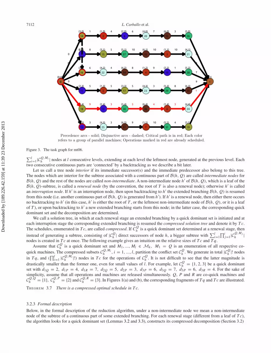
We represent each feasible solution σh by a directed weighted graph Gh . We associate the digraph (task graph)G0 = (X, E0) with the root of T (see also later Figure 3). To each task i ∈ O , there corresponds the unique node i ∈ X .There is one fictitious initial node 0, preceding all nodes, and one fictitious terminal node n + 1 succeeding all nodes in G0.E0 is the arc set consisting of the arcs (i, j) for each task i , directly preceding task j ; (0, i) ∈ E0 if task i has no predecessorsand ( j, n + 1) ∈ E0 if task j has no successors. We denote by w(i, j) the weight associated with (i, j) ∈ E0; initially, weassign to w(i, j) the minimal processing time of task i later we correct these weights when we assign a task to the particularprocessor.
Let (h, h′) be an edge in T with task j scheduled at iteration h′ on processor P . Then, we obtain Gσh′ from Gσh as follows.We complete the arc set of the latter graph with the arcs of the form (i, j), with the associated weights w(i, j) = di P , foreach task i , scheduled earlier on the processor P . We correct the weights of all arcs incident out from node j ( j, o) ∈ E0, asw( j, o) := d j P . It is easily seen that the length of a critical path in Gh′ is the makespan of the (partial or complete) solutionσh′ = σh j P which we denote by |σh′ |.
Note that the critical path length from node 0 to a node o in Gh is a lower bound on the starting time of operation o inschedule σh and in any of its successor schedules. We call it the earliest starting time or the head of operation o by stageh and denote it by headh(o). Likewise, the critical path length from o to the sink node in Gh is a lower bound on the totalremained work once operation o is already finished. We denote it by tailh(o) and call it the tail of operation o at stage h.Rh(M) is the release time of machine M at stage h, that is the completion time of the operation, scheduled last by that stageon M .
3. The reduction algorithm
In this section, we give a compact but complete description of the reduction algorithm which is based on the conceptspresented in Vakhania and Shchepin (2002). We need to introduce formally some earlier mentioned notions as well as somenew concepts to give a formal description of the algorithm. For self-completeness of the presentation, we also give the basicproperties on which the algorithm relies. Further details and the proofs of these properties (lemmas and theorems from thissection) can be found in Vakhania and Shchepin (2002).
3.1 Phase 1: constructing the quick solution tree
In this subsection, we describe how the preliminary reduction of the feasible solution space is accomplished in Phase 1 ofthe reduction algorithm. Recall that Phase 1 is common for both JSP and MJSP.
Dow
nloa
ded
by [
189.
226.
42.1
59]
at 1
1:39
23
Dec
embe
r 20
13

International Journal of Production Research 7109
3.1.1 Dominance relations for creating active schedules
We first describe the dominance relations which have been traditionally used for a preliminary reduction of the whole feasiblesolution set for JSP. Let us denote by Okh the subset of operations of Ok , not yet scheduled by stage h. Let o be a readyoperation from Okh and p be another operation from Okh , such that headh(o) ≤ headh(p). We will say that o conflicts withp on machine M ∈ Mk at stage h if the overlapping of the execution times of o and p on M is more than one point, i.e. ocannot be completed on M before or at the earliest starting time of p at stage h. If o does not conflict with p, then o dominatesp, written o domMh p (o can be completed on M before or at the earliest moment when p can be started on M). Thus, if oconflicts with p on M , then by scheduling o on M , we will delay the starting of p on M ; otherwise, we will not delay thestarting of p.
Let k be a machine group with at least one ready operation in Okh , M ∈ Mk and let o be a ready operation in Okh withthe minimal earliest completion time on M . Then the set of operations, consisting of operation o and all the operations ofOkh , conflicting with o on M , is called the conflict set on M at stage h and is denoted by CM
h .Operation o may conflict with operation p on machine M , but may not conflict on another machine Q. We illustrate
this by the following simple example. Let {1, 2, 3} be ready operations with headh(1) = 5, headh(2) = 6, headh(3) = 8,d1Q = 2, d1M = 6, d2Q = 5, d2M = 3, d3Q = 2, d3M = 7. Assume that Rh(Q) = Rh(M) = 5. Observe that CQ
h = {1, 2}and CM
h = {1, 2, 3}, since 1 domQh 3, though not 1 domMh 3. However, if, for example, we change d1Q to 4, or we leaved1Q unchanged, but we change the release time of Q to 7, then 1 will no more dominate 3 on machine Q. Thus, for distinctM and Q, the conflict sets CM
h and CQh are not necessarily the same (though both sets will contain all ready operations with
the minimal head).If a conflict set CM
h contains at least one non-ready operation p, then we are not allowed to branch by this set. Moreover,by ignoring operation p we may loose the optimal schedule (since p would be delayed on M in any generated schedule).We are allowed to branch by CM
h if it contains no non-ready operation; in this case, we shall call it a dominant conflict set onmachine M at iteration h. Observe that in a dominant set CM
h , the operation o with the minimal earliest completion time onmachine M dominates all operations of Okh which are not in CM
h (if there exist such operations); in this case, we will saythat CM
h is dominant by operation o. We call σhoM a dominant extension of σh , if o belongs to a dominant set on M at stageh.
A partial schedule σh dominates another partial schedule σh′ , if there exists at least one complete extension σ of σh suchthat τ(σ ) ≤ τ(σ ′) for any complete extension σ ′ of σh′ . Let CM
h be a dominant conflict set and o be its operation with theminimal head. Recall that CM
h contains no ready operation p ∈ Okh dominated by o. However, σh pM is a feasible extensionof σh . The following lemma shows that this feasible extension can be ignored.
Lemma 3.1 σhoM dominates σh pM . Hence, if the branching is carried out by the dominant set CMh , then σh pM can be
abandoned at stage h.
Let us call a machine Q ∈ Mk quick at stage h for a ready operation o ∈ Okh if the earliest completion time of thisoperation on machine Q is no more than that on any other machine of Mk at stage h. In the sequel, we will use the followingsimple method to generate a dominant conflict set at each stage h.
Lemma 3.2 If o is a ready operation at stage h with the minimal earliest completion time and Q is the correspondingquick machine, then the conflict set CQ
h is dominant.
3.1.2 Quick solution tree
As already mentioned, the dominant conflict sets have been traditionally used in JSP for branching. In an active schedule, nooperation can be completed earlier than it is scheduled (by altering the processing order of the operations on the machines)without delaying some other operation. It can be easily seen that the schedules, generated by branching at each stage bya dominant conflict set, are active (see Lageweg, Lenstra, and Rinnooy Kan (1977) for the details). Thus, so far, we haveextended the common branching rule for generating active schedules of JSP for MJSP in a straightforward way: it is clearthat it suffices to generate all possible dominant extensions of σh corresponding to all dominant conflict sets of stage h, i.e.active schedules of MJSP.
Observe that the number of dominant conflict sets might be the same as that of the parallel machines of the correspondinggroup. We will now show that it is always possible to generate only extensions corresponding to just one of the dominantconflict sets, generalising in this way the concept of an active schedule for MJSP.
The branchings, generated at each stage, restrict the set of feasible solutions which will be created in T in the followingsense. Suppose we carry out the branching only by a conflict set CM
h at stage h. Then, in any feasible solution created inT , at least one operation of CM
h will be scheduled next on machine M . It is easy to see that, if we arbitrarily select a single
Dow
nloa
ded
by [
189.
226.
42.1
59]
at 1
1:39
23
Dec
embe
r 20
13

7110 L. Carballo et al.
dominant conflict set for branching, we may loose an optimal schedule. For example, assume that CQh = CM
h = {1, 2} aretwo dominant conflict sets at stage h. Let headh(1) = 4 and headh(2) = 5, d1Q = 2, d1M = 6 and d2Q = 3, d2M = 7. Itis clear that both operations should be scheduled on machine Q, while, if we branch at stage h only by the set CM
h , then atleast one of these operations will be scheduled on machine M and the optimal schedule will be lost.
We select a single dominant set and discard the rest of the dominant sets with a little computational effort. Let us call aconflict set CQ
h quick at stage h by operation o ∈ CQh if Q is a quick machine for o; that is, any conflict set on a machine,
which is quick for at least one its operation, forms a quick conflict set.
Lemma 3.3 A dominant conflict set according to Lemma 3.2 is quick.
Let us call a quick solution tree a solution tree, in which the branching at each stage is carried out by a single quickdominant conflict set. Similarly, we shall refer to a solution tree, in which the branching at each stage is carried out by alldominant conflict sets as an active solution tree. We use T q and T a to denote quick and active solution trees, respectively.An active solution tree enumerates all active schedules, while a quick solution tree enumerates a subset of active schedules,the so-called quick schedules. Observe that for JSP, quick and active solution trees coincide:
Proposition 3.4 A quick solution tree for an instance of JSP enumerates all active schedules for this instance.
Theorem 3.5 There is an optimal schedule in T q for any instance of MJSP.
As we will see in the example in Section 3.2, different conflict sets CMh , M ∈ Mk , may contain a different number of
operations. Intuitively, the lower is the minimal earliest operation completion time in a conflict set, the less is the number ofoperations in this set. In this sense, the quick dominant set of Lemma 3.2 contains a potentially small number of operations.
We associate an instance of JSP with an instance of MJSP. In an instance of JSP, associated with the instance of MJSP, asingle machine M ∈ Mk for k = 1, ..., m, is selected and the processing time of each operation o ∈ Ok is set to doM . Observethat, if no two alternative machines are identical, then there are in total
∏mk=1 |Mk | problem instances of JSP associated with
an instance of MJSP.
Theorem 3.6 A quick solution tree T q, generated for an instance of MJSP, has no more nodes than an active solution treeT a, generated for any associated instance of JSP.
3.2 Phase 2: further reduction of the solution space for MJSP
In this subsection, we describe Phase 2 of the reduction algorithm that drastically reduces the size of the solution space ofinstances of MJSP.
3.2.1 Partitioning conflict sets
In a branch-and-bound solution tree of JSP, we commonly branch by all operations of a conflict set to provide a non-delaystarting of each of these operations (since in an optimal schedule, we may need potentially to schedule any of these operationswithout any delay). If we do not branch by some operation of a conflict set (and branch by the rest of the operations of theconflict set), then that operation cannot be started at its earliest starting time in any subsequently obtained complete feasibleschedule, which may cause the loss of the optimal schedule. The situation is less restricted if there are two or more parallelmachines in Mk : it might be possible to postpone the branching by some operations of the conflict set to a later stage withoutdelaying the start of these operations.
Let CQh be a quick dominant set. We wish to partition CQ
h into smaller subsets and branch by these smaller subsetsinstead of branching by the whole conflict set CQ
h at stage h. To partition the conflict set, we look for quick machines forthe operations in CQ
h . The number of subsets in the partition is equal to the maximal number of pairs of the form (o, M),o ∈ CQ
h , M ∈ Mk , such that M is a quick machine for o and no o or M is encountered more than once in any two or morepairs. Roughly speaking, we keep a similar number of operations in each subset of the partition to minimise the number ofgenerated schedules. To be more specific, with each operation o ∈ CQ
h a (non-empty) set of its quick machines is associated.We wish to find the maximal subset of CQ
h for each operation of which a different quick machine is selected. This selectionproblem is equivalent to the maximal matching problem in a bipartite graph G = (V1, V2, E) with V1 = CQ
h , V2 = Mk ,where there is an edge (o, M) in E if and only if M is a quick machine for operation o at iteration h. This problem is solvablein O(
√|V1||E |) time, see Hopcroft and Karp (1973). Suppose Omaxh is a maximal matching, i.e. a maximal subset of CQ
h , foreach operation of which a distinct quick machine is selected (note that |Omax
h | > 0). We call machine M a co-quick machineof iteration h if M is selected for some operation of Omax
h .
Dow
nloa
ded
by [
189.
226.
42.1
59]
at 1
1:39
23
Dec
embe
r 20
13

International Journal of Production Research 7111
(a) (b)
Figure 1. Corresponding fragments of (a) T q and (b) T c.
Figure 2. Graphical user interface.
We partition CQh into |Omax
h | subsets, such that we have exactly one operation from Omaxh in each subset. The total
number of operations in each subset is either [|CQh |/|Omax
h |] or [|CQh |/|Omax
h |] + 1; for the latter option |CQh |/|Omax
h | is notintegral, and the subsets with [|CQ
h |/|Omaxh |]+1 elements are selected arbitrarily. We call the partition of CQ
h , obtained in thisway, a compressed decomposition of CQ
h . Observe that with each subset in the decomposition, a unique co-quick machineis associated. We denote by CQ,M
h the subset in the decomposition with the associated machine M and call it a compressedsubset of CQ
h at stage h.
3.2.2 Extended branching and the compressed solution tree
Let CQ,Mih , i = 1, ..., l, l = |Omax
h | be an enumeration of the elements of a compressed decomposition of the dominantquick set CQ
h . Instead of branching by the whole set CQh at stage h, we branch by subsets of its compressed decomposition
on consecutive levels of the solution tree T . We call such a branching, extended at different levels of the tree, an extendedbranching by the set CQ
h and the decomposition CQ,Mih and we denote it by B(h, Q) (we omit the term CQ
h for notationalsimplicity). The corresponding subtree will be referred to as the B(h, Q)-subtree (the root of this subtree is the node h).B(h, Q) originates in total
∏li=1|CQ,Mi
h | different paths (leaves of the B(h, Q)-subtree). It allocates operations of CQ,Mih on
machine Mi at the i th level of the B(h, Q)-subtree extending all generated nodes of level i − 1 (extending the root of theB(h, Q)-subtree initially). So, there are
∏il=1|CQ,Ml
h | nodes at the i th level of the B(h, Q)-subtree. While enumerating ourschedules, the B(h, Q)-subtree is not generated in a continuous manner. B(h, Q) consists of different continuous parts, i.e.continuously generated subtrees of the B(h, Q)-subtree. The first continuous part of B(h, Q) starts at stage h and generates
Dow
nloa
ded
by [
189.
226.
42.1
59]
at 1
1:39
23
Dec
embe
r 20
13
7112 L. Carballo et al.
Figure 3. The task graph for mt06.
∑li=1|CQ,Mi
h | nodes at l consecutive levels, extending at each level the leftmost node, generated at the previous level. Eachtwo consecutive continuous parts are ‘connected’ by a backtracking as we describe a bit later.
Let us call a tree node interior if its immediate successor(s) and the immediate predecessor also belong to this tree.The nodes which are interior for the subtree associated with a continuous part of B(h, Q) are called intermediate nodes forB(h, Q) and the rest of the nodes are called non-intermediate. A non-intermediate node h′ of B(h, Q), which is a leaf of theB(h, Q)-subtree, is called a renewal node (by the convention, the root of T is also a renewal node); otherwise h′ is calledan interruption node. If h′ is an interruption node, then upon backtracking to h′ the extended branching B(h, Q) is resumedfrom this node (i.e. another continuous part of B(h, Q) is generated from h′). If h′ is a renewal node, then either there occursno backtracking to h′ (in this case, h′ is either the root of T , or the leftmost non-intermediate node of B(h, Q), or it is a leafof T ), or upon backtracking to h′ a new extended branching starts from this node; in the latter case, the corresponding quickdominant set and the decomposition are determined.
We call a solution tree, in which at each renewal stage an extended branching by a quick dominant set is initiated and ateach interruption stage the corresponding extended branching is resumed the compressed solution tree and denote it by T c.The schedules, enumerated in T c, are called compressed. If C Q
h is a quick dominant set determined at a renewal stage, then
instead of generating a subtree, consisting of |CQh | direct successors of node h, a bigger subtree with
∑li=1
∏ij=1|CQ,M j
h |nodes is created in T c at once. The following example gives an intuition on the relative sizes of T c and T q.
Assume that CQh is a quick dominant set and M1, ..., Ml ∈ Mk, M1 = Q is an enumeration of all respective co-
quick machines. The compressed subsets CQ,Mih , i = 1, ..., l, partition the conflict set CQ
h . We generate in total |CQh |! nodes
in T q , and (∏l
i=1 |CQ,Mih |!) nodes in T c for the operations of CQ
h . It is not difficult to see that the latter magnitude isdrastically smaller than the former one, even for small values of l. For example, let CQ
h = {1, 2, 3} be a quick dominantset with d1Q = 2, d1P = 4, d1R = 7, d2Q = 5, d2P = 3, d3P = 6, d3Q = 7, d3P = 6, d3R = 4. For the sake ofsimplicity, assume that all operations and machines are released simultaneously. Q, P and R are co-quick machines andCQ,Q
h = {1}, CQ,Ph = {2} and CQ,R
h = {3}. In Figures 1(a) and (b), the corresponding fragments of T q and T c are illustrated.
Theorem 3.7 There is a compressed optimal schedule in T c.
3.2.3 Formal description
Below, in the formal description of the reduction algorithm, under a non-intermediate node we mean a non-intermediatenode of the subtree of a continuous part of some extended branching. For each renewal stage (different from a leaf of T c),the algorithm looks for a quick dominant set (Lemmas 3.2 and 3.3), constructs its compressed decomposition (Section 3.2)
Dow
nloa
ded
by [
189.
226.
42.1
59]
at 1
1:39
23
Dec
embe
r 20
13

International Journal of Production Research 7113
1. COMPRESSION-ALGORITHM()
1: h := 0; {initial settings}2: R := succ(0); {set the current set of the ready operations}3: while R �= ∅ or there exists a retreat node do4: if R �= ∅ then5: if h is a renewal node then6: {form a quick dominant set and its compressed decomposition}7: o := a ready operation with the minimal completion time at stage h;8: Q := a quick machine for o;
9: CQh := the conflict set (include in it operation o and all ready operations, which conflict with o on Q);
10: CQ,Mih := a compressed decomposition, i = 1, ..., l, of CQ
h ;11: B(h, Q); {call to generate the first continuous part of the extended branching}12: h′ := the retreat node;13: SCHEDULE(h, h′);14: h := h′;15: else16: {h is an interruption node of some extended branching, say B}17: B(h, Q); {carry out the next continuous part of the extended branching B from node h}18: h′ := the retreat node;19: SCHEDULE(h, h′);20: h := h′;21: end if22: else23: σh := is the current complete solution;{i.e., a complete solution is obtained}24: σopt := is the best complete solution at this moment;25: if there exists a retreat node then26: h′ := the retreat node;27: h := father(h′);28: SCHEDULE(h, h′);29: h := h′;30: end if31: end if32: end while33: return σopt ;
2. SCHEDULE(h, h′) schedule each operation, associated with an edge on the path from node h to node h′
1: for all edge of the path from node h to node h′ in Th′ do2: o := operation associated with this edge;3: M := machine associated with this edge;4: R := R ∪ succ(o); {add to the current set of the ready operations the ones from succ(o)}5: R := R − o; {delete operation o from the set R}6: for all p ∈ σh, already scheduled on machine M do7: Gh′ := Gh ∪ (p, o);8: w(p, o) := dpM ;9: end for
10: for all p ∈ succ(o) do11: w(o, p) := doM ;12: end for13: end for
and starts the extended branching by this decomposition, i.e. it generates its first (leftmost) continuous part. Each time anew complete solution is generated, the backtracking to the leftmost non-intermediate node of the highest level (less thann) is performed (the latter node will be referred to as the retreat node). Whenever we backtrack, we either resume an earlierinterrupted extended branching (the retreat node is an interruption node) or we initiate a new extended branching (the retreatnode is a renewal node). succ(o) denotes the set of immediate successors of operation o.
Dow
nloa
ded
by [
189.
226.
42.1
59]
at 1
1:39
23
Dec
embe
r 20
13

7114 L. Carballo et al.
Figure 4. A fragment of the compressed solution tree for mt06.
Observation 3.8 Let ν and μ, respectively, be an upper limit on the number of operations and machines, respectively, ineach group. The cost spent at each node of T c is determined by Step 1c and is of the order O(ν
√νμ).
4. Computational experiments
We have implemented the reduction algorithm in C++ using the IDE Qt Creator v.2.4.1 on a computer equipped with 8 GBof RAM, AMD Phenom (tm) II X6 1100T x6 Processor and operating system Ununtu 12.04 to 64-bit. The implementedsoftware has three different threads. The main thread takes care of the graphical part representing all data, including theproblem data, all the necessary intermediate results from the reduction algorithm available for the user and the interactionwith the user (Figure 2 illustrates some of these data). Figures 3 and 4 illustrate the graphical representation used in the mainthread of task graphs and solution trees. The second thread executes the reduction algorithm. The third auxiliary thread servesas an intermediate thread between the main thread and the second thread. In particular, whenever an intermediate result fromthe second thread is available, the third auxiliary thread informs the main thread about such an event. Then, the main threadupdates the corresponding graphical data.
The user may have two different modes for the interaction with the software. The debugger mode provides a step-by-stepupdate from the reduction algorithm (concerning basic constructions such as dominant and conflict groups, compresseddecomposition, scheduling the operations, the determination of the critical path, the current state of the solution tree, etc.).Alternatively, the user may only ask for updates on the total number of the feasible solutions generated so far and when anew complete solution, better than the earlier best one is created. The access to this data is provided by the third auxiliarythread, and it is optional.
We have based on a number of instances of JSP. In particular, the three classical instances with 6 jobs on 6 machines(mt06), 20 jobs on 5 machines (mt20) and 10 jobs on 10 machines (mt10) were taken from Fisher and Thompson (1963).The other five JSP instances were taken from Lawrence (1984) with 10 jobs on 5 machines (la01-la05), and five moreinstances were taken from the same reference with 15 jobs on 5 machines (la06-la10). The last two instances are fromAdams, Balas, and Zawack (1988) with 10 jobs on 10 machines (abz5 and abz6).
In all these JSP instances (which are also available in the OR-Library), every job has exactly one operation on each ofthe machines. Based on them, we have generated instances of MJSP. Each machine in the corresponding instance of JSPwas replaced by a group of parallel machines. The number of parallel machines in every group is the same integer number.In each generated instance of MJSP, the original operation processing times are assigned to every first machine of each
Dow
nloa
ded
by [
189.
226.
42.1
59]
at 1
1:39
23
Dec
embe
r 20
13
International Journal of Production Research 7115
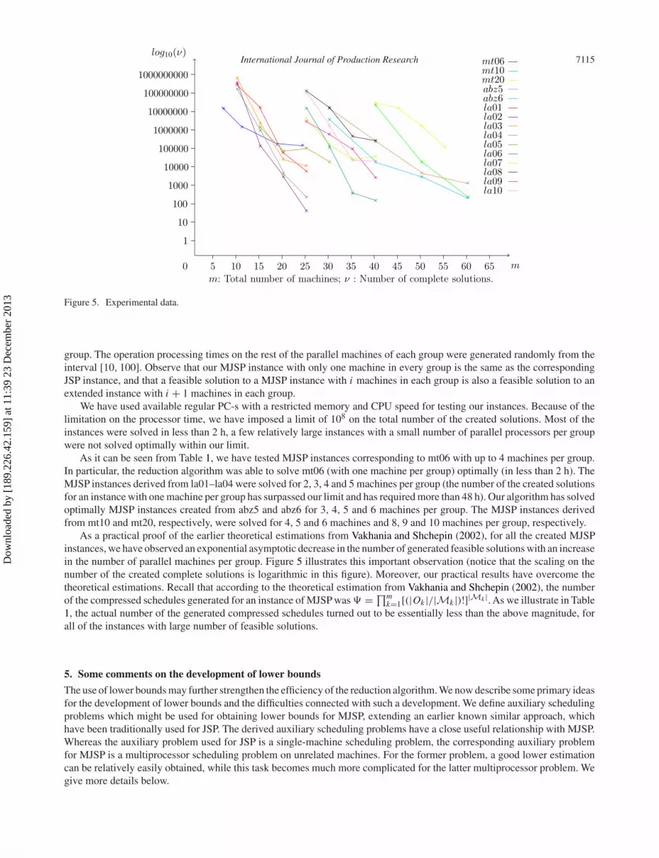
Figure 5. Experimental data.
group. The operation processing times on the rest of the parallel machines of each group were generated randomly from theinterval [10, 100]. Observe that our MJSP instance with only one machine in every group is the same as the correspondingJSP instance, and that a feasible solution to a MJSP instance with i machines in each group is also a feasible solution to anextended instance with i + 1 machines in each group.
We have used available regular PC-s with a restricted memory and CPU speed for testing our instances. Because of thelimitation on the processor time, we have imposed a limit of 108 on the total number of the created solutions. Most of theinstances were solved in less than 2 h, a few relatively large instances with a small number of parallel processors per groupwere not solved optimally within our limit.
As it can be seen from Table 1, we have tested MJSP instances corresponding to mt06 with up to 4 machines per group.In particular, the reduction algorithm was able to solve mt06 (with one machine per group) optimally (in less than 2 h). TheMJSP instances derived from la01–la04 were solved for 2, 3, 4 and 5 machines per group (the number of the created solutionsfor an instance with one machine per group has surpassed our limit and has required more than 48 h). Our algorithm has solvedoptimally MJSP instances created from abz5 and abz6 for 3, 4, 5 and 6 machines per group. The MJSP instances derivedfrom mt10 and mt20, respectively, were solved for 4, 5 and 6 machines and 8, 9 and 10 machines per group, respectively.
As a practical proof of the earlier theoretical estimations from Vakhania and Shchepin (2002), for all the created MJSPinstances, we have observed an exponential asymptotic decrease in the number of generated feasible solutions with an increasein the number of parallel machines per group. Figure 5 illustrates this important observation (notice that the scaling on thenumber of the created complete solutions is logarithmic in this figure). Moreover, our practical results have overcome thetheoretical estimations. Recall that according to the theoretical estimation from Vakhania and Shchepin (2002), the numberof the compressed schedules generated for an instance of MJSP was � = ∏m
k=1[(|Ok |/|Mk |)!]|Mk |. As we illustrate in Table1, the actual number of the generated compressed schedules turned out to be essentially less than the above magnitude, forall of the instances with large number of feasible solutions.
5. Some comments on the development of lower bounds
The use of lower bounds may further strengthen the efficiency of the reduction algorithm. We now describe some primary ideasfor the development of lower bounds and the difficulties connected with such a development. We define auxiliary schedulingproblems which might be used for obtaining lower bounds for MJSP, extending an earlier known similar approach, whichhave been traditionally used for JSP. The derived auxiliary scheduling problems have a close useful relationship with MJSP.Whereas the auxiliary problem used for JSP is a single-machine scheduling problem, the corresponding auxiliary problemfor MJSP is a multiprocessor scheduling problem on unrelated machines. For the former problem, a good lower estimationcan be relatively easily obtained, while this task becomes much more complicated for the latter multiprocessor problem. Wegive more details below.
Dow
nloa
ded
by [
189.
226.
42.1
59]
at 1
1:39
23
Dec
embe
r 20
13

7116 L. Carballo et al.
Table 1. Experimental results.
p n g � μ m ν Cmax
mt06 6 6
15399682740640811135241 1 6 15873751 55244140625 2 12 1865676 51
117649 3 18 202269 47729 4 24 158562 47
mt10 10 10282475249 4 40 59163287 292282475249 5 50 20497 253
59049 6 60 341 211
mt20 20 5
16807 8 40 56539895 13516807 9 45 15854040 12516807 10 50 1349739 9816807 11 55 102846 90
abz5 10 1095367431640625 3 30 13746407 461
282475249 4 40 262156 365282475249 5 50 6919 336
59049 6 60 1135 291
abz6 10 10
95367431640625 3 30 6559490 451282475249 4 40 30670 366282475249 5 50 4884 355
59049 6 60 282 321
la01 10 5
194839193667601 2 10 510468511 3459765625 3 15 17961150 234
16807 4 20 77304 20516807 5 25 7249 192
la02 10 5
194839193667601 2 10 618596793 3499765625 3 15 194138 214
16807 4 20 5208 19216807 5 25 65 167
la03 10 5
194839193667601 2 10 904394870 3049765625 3 15 3826177 192
16807 4 20 42362 17616807 5 25 13215 164
la04 10 5
194839193667601 2 10 244483378 3059765625 3 15 1015814 221
16807 4 20 6673 17916807 5 25 389 174
la05 10 5
9765625 3 15 2821538 22516807 4 20 82560 18516807 5 25 107956 176
243 6 30 29931 145
la06 15 5
9765625 5 25 14591953 17216807 6 30 145889 15116807 7 35 681 15116807 8 40 206 151
(Continued)
Dow
nloa
ded
by [
189.
226.
42.1
59]
at 1
1:39
23
Dec
embe
r 20
13

International Journal of Production Research 7117
Table 1. (Continued).
la07 15 5
9765625 5 25 7525885 17216807 6 30 312414 16816807 7 35 47662 15616807 8 40 56469 156
la08 15 5
9765625 5 25 175925311 19816807 6 30 18492889 16916807 7 35 670404 16916807 8 40 538148 141
la09 15 5
9765625 5 25 4039015 20316807 6 30 706916 18616807 7 35 90341 18616807 8 40 3732 186
la10 15 5
9765625 5 25 108813452 19616807 6 30 2230028 17516807 7 35 43971 14316807 8 40 36021 143
Note: p: Problem instance; μ: Number of machines per group; n: Number of jobs; m: Total number of machines; g: Number of groupsof parallel machines; ν: Number of complete solutions; Cmax: makespan value; � Theoretical estimation from Vakhania and Shchepin(2002)
Remind that in a branch-and-bound scheme, if a lower bound L(σh) of the partial solution σh is larger than or equal tothe makespan |σ | of some already generated complete solution σ (a current upper bound), then all extensions of σh can beabandoned. Clearly, L(σh) cannot be larger than the makespan of the best potential extension of σh (otherwise we couldloose this extension). At the same time, we try to make it as close as possible to this value: then the chances are larger thatL(σh) ≥ |σ |). Let σh ∈ T and o ∈ Ch for an instance of MJSP. We would like to obtain a lower bound for an extension of σh
with operation o scheduled on machine Q ∈ Mk , σhoQ ∈ T . A trivial lower bound is LT (σhoQ) = |σh | + tailh(o), where|σh | is the makespan of σh , i.e. the critical path length in Gh . Note that the remained work determined by tailh(o) reflectsall the original precedence constraints and all the resource constraints which have been resolved so far by stage h. So, thisbound ignores all yet unresolved potential conflicts, i.e. the processing times of yet unscheduled tasks.
It is easy and fast to obtain LT , but it is clear that one cannot get a good estimation of the desired optimal makespanby the complete ignorance of the potential contribution of the unscheduled tasks. A stronger lower bound would take intoaccount a possible contribution of the latter tasks (which would obviously require additional computational efforts). Clearly,we cannot know in advance how yet unresolved conflicts will be resolved in an optimal schedule. But, we can make someassumptions about this (‘simulating’ in advance some ‘future’ resource constraints). However, we should be careful since weare not allowed to violate the condition L(σh) ≤ |σ ′|, σ ′ being an arbitrary complete extension of σh . Roughly speaking, wewould like to have a lower estimation on how the future resource conflicts will be resolved; this will involve some optimalscheduling on parallel machines.
Now we derive an auxiliary multiprocessor scheduling problem which we use for our lower bounds. For JSP, themost commonly used is a one-machine relaxation (for e.g. see Adams, Balas, and Zawack 1988, Blazewicz et al. 1986,Carlier and Pinson 1989, Lageweg, Lenstra, and Rinnooy Kan 1977, McMahon and Florian 1975): all resource constraintsare relaxed (ignored) except the ones of one particular (not yet completely scheduled) machine, and the resulting one-machine problem 1|ri , qi |Cmax with heads and tails is then solved. A bottleneck machine is one which results in the maximalmakespan among all yet unscheduled machines (intuitively, a bottleneck machine gives a maximal expected contribution inthe makespan of extensions of σh). This approach can be generalised as follows. Basically, we relax the resource constraintson all machines except the ones from some (bottleneck) set of the machines Mk .
To be specific, let at iteration h, |Okh | ≥ 2, where Okh is the subset of Ok consisting of the tasks not yet scheduledby stage h; i.e. we have yet unresolved resource constraints associated with the machines of Mk . An operation i ∈ Okh ischaracterised by its earliest starting (release) time headh(i) and tail tailh(i); that is, i cannot be started earlier than at timeheadh(i), and once it is completed it will take at least tailh(i) time for all successors of i to be finished. Operation i can bescheduled on any of the machines of Mk and has a processing time di P on machine P ∈ Mk . Each machine P ∈ Mk hasits release time Rh(P).
Dow
nloa
ded
by [
189.
226.
42.1
59]
at 1
1:39
23
Dec
embe
r 20
13

7118 L. Carballo et al.
Observe that the operation tails and release times are derived from Gh (this ignores all resource constraints unresolvedby stage h). Besides, the tails require no machine time, i.e. no time on any of the machines of Mk . We are looking for anoptimal (i.e. minimising the makespan with tails) ordering of the operations of Okh on the machines from Mk under theconditions stated above. Thus, for each stage h for the partial solution σh , the auxiliary problem of scheduling tasks withrelease times and tails on a group of parallel machines Mk with the objective to minimise the makespan has been obtained.We denote this auxiliary problem by Akh and the respective optimal makespan by |Akh |.
Let μh be the set of indexes of all machine groups such that for each k ∈ μh , |Okh | ≥ 2. It is clear that |Akh |, for anyk ∈ μh , is a lower bound for node h. We may find all |μk | ≤ m lower bounds for node h and take the maximum, thus findinga bottleneck machine group. Thus, instead of dealing with the problem 1|ri , qi |Cmax in the case of JSP, now we deal with theproblem R|ri , qi |Cmax. Both problems are NP-hard, though there exist exponential algorithms with a good practical behaviourfor the first above problem, have been commonly used in one-machine relaxation based branch-and-bound algorithms forJSP (see, e.g., Carlier 1982, Carlier and Pinson 1989 and McMahon and Florian 1975). Unfortunately, there are no knownalgorithms with a good practical performance for the problem P|ri , qi |Cmax (the version with identical machines) and soalso for the problems Q|ri , qi |Cmax and R|ri , qi |Cmax. Some additional ideas for obtaining lower bounds for these problemsare given in Carballo, Vakhania, and Werner (2013).
6. Concluding remarks
We see the following basic directions for further relevant research. First, the lower bounds proposed in Section 5 and inCarballo, Vakhania, and Werner (2013) might be tested independently and compared with each other, both in efficiency andin the required computational efforts. This may yield an implicit enumeration algorithm for MJSP, more efficient than thereduction algorithm.
At the same time, a further theoretical improvement of some of the proposed bounds might be possible. In this connection,we have to look for alternative, more efficient algorithms for the problems R|ri , qi |Cmax, Q|ri , qi |Cmax (or their preemptiveversions), or even for the problem R||Cmax, Q||Cmax (or their preemptive versions).
The reduction algorithm and the proposed bounds may serve as a basis for sophisticated heuristic algorithms. In particular,the reduced solution tree constructed by our algorithm may well serve for a filtered beam search algorithm using our non-strictbounds.
The presented framework can be aggregated by an additional graph-completion mechanism for taking into accounttransportation and setup times.
References
Adams, J., E. Balas, and D. Zawack. 1988. “The Shifting Bottleneck Procedure for Job Shop Scheduling.” Management Science 34:391–401.
Blazewicz, J., W. Cellary, R. Slowinski, and J. Weglarz. 1986. “Scheduling Under Resource Constraints – Deterministic Models.” Annalsof Operations Research 7: 1–350.
Brucker, P., B. Jurisch, and A. Krämer. 1997. “Complexity of Scheduling Problems with Multi-purpose Machines.” Annals of OperationsResearch 70: 57–73.
Brucker, B., and R. Schlie. 1990. “Job Shop Scheduling with Multi-purpose Machines.” Computing 45: 369–375.Carballo, L., N. Vakhania, and F. Werner. 2013. A Comparative Study of the Effect of the Preliminary Reduction for the Classical and
Multiprocessor Job-Shop Problems. Preprint 05/13. OvGU Magdeburg: FMA, 23.Carlier, J. 1982. “The One-machine Sequencing Problem.” European Journal of Operational Research 11: 42–47.Carlier, J., and E. Pinson. 1989. “An Algorithm for Solving Job Shop Problem.” Management Science 35: 164–176.Dauzère-Pérès, S., and J. Paulli. 1997. “An IntegratedApproach for Modeling and Solving the General Multiprocessor Job Shop Scheduling
Problem with Tabu Search.” Annals of Operations Research 70: 281–306.Fisher, H., and G. L. Thompson. 1963. “Probabilistic Learning Combinations of Local Job-Shop Scheduling Rules.” In Industrial
Scheduling, edited by J. F. Muth and G. L.Thompson, 225–251. Englewood Cliffs, NJ: Prentice Hall.Giffler, B., and G. L. Thompson. 1960. “Algorithm for Solving Production Scheduling Problems.” Operations Research 8: 487–503.Gröflin, H., and A. Klinkert. 2008. “Feasible Job Insertions in the Multi-processor-task Shop.” European Journal of Operational Research
185: 1308–1318.Hopcroft, J. E., and R. M. Karp. 1973. “A n5/2 Algorithm for Maximum Matching in Bipartite Graphs.” SIAM Journal of Computing 2:
225–231.Huang, R. H., and S. C. Yu. 2011. “Multi-processor Job Shop Scheduling with Due Windows.” In IEEE Conference on Industrial
Engineering and Engineering Management. Singapore.
Dow
nloa
ded
by [
189.
226.
42.1
59]
at 1
1:39
23
Dec
embe
r 20
13

International Journal of Production Research 7119
Ivens, P., and M. Lambrecht. 1996. “Extending the Shifting Bottleneck Procedure to Real-life Applications.” European Journal ofOperational Research 90: 252–268.
Jurisch, B. 1995. “Lower Bounds for Job-shop Scheduling Problem on Multi-purpose Machines.” Discrete Applied Mathematics 58:145–156.
Lageweg, B. J., J. K. Lenstra, and A. H. G. Rinnooy Kan. 1977. “Job Shop Scheduling By Implicit Enumeration.” Management Science24: 441–450.
Lawrence, S. 1984. Resource Constrained Project Scheduling: An Experimental Investigation of Heuristic Scheduling Techniques(Supplement). Graduate School of Industrial Administration: Carnegie-Mellon University, Pittsburgh, Pennsylvania.
McMahon, G. B., and M. Florian. 1975. “On Scheduling with Ready Times and Due Dates to Minimize Maximum Lateness.” OperationsResearch 23: 475–482.
Mousakhani, M. 2013. “Sequence-dependent Setup Time Flexible Job Shop Scheduling Problem to Minimize Total Tardiness.”International Journal of Production Research 51: 3476–3487.
Ow, P. S., and T. E. Morton. 1988. “Filtered Beam Search in Scheduling.” International Journal of Production Research 26: 35–62.Schutten, J. M. J. 1998. “Practical Job Shop Scheduling.” Annals of Operations Research 83: 161–177.Shmoys, D. B., C. Stein, and J. Wein. 1994. “Improved Approximation Algorithms for Shop Scheduling Problems.” SIAM Journal on
Computing 23: 617–632.Sotskov, Y. N., T. Tautenhahn, and F. Werner. 1999. “On the Application of Insertion Techniques for Job Shop Problems with Setup Times.”
RAIRO Recherche Operationelle-Operations Research 33: 209–245.Tanaev, V. S., Y. N. Sotskov, and V. A. Strusevich. 1994. Scheduling Theory: Multi-stage Systems, 1–420. Dordrecht: Springer.Vakhania, N. 1995. “Assignment of Jobs to Parallel Computers of Different Throughput.” Automation and Remote Control 56: 280–286.Vakhania, N. 2000. “Global and Local Search for Scheduling Job Shop with Parallel Machines.” Lecture Notes in Artificial Intelligence
(IBERAMIA-SBIA 2000) 1952: 63–75.Vakhania, N., and E. Shchepin. 2002. “Concurrent Operations can be Parallelized in Scheduling Multiprocessor Job Shop.” Journal of
Scheduling 5: 227–245.Wang, L., S. Wang, and M. Liu. 2013. “A Pareto-based Estimation of Distribution Algorithm for the Multi-objective Flexible Job-Shop
Scheduling Problem.” International Journal of Production Research 51: 3574–3592.Werner, F., and A. Winkler. 1995. “Insertion Techniques for the Heuristic Solution of the Job Shop Problem.” Discrete Applied Mathematics
58: 191–211.Zhang, L., L. Gao, and X. Li. 2013. “A Hybrid Genetic Algorithm and Tabu Search for a Multi-objective Dynamic Job Shop Scheduling
Problem.” International Journal of Production Research 51: 3516–3531.
Dow
nloa
ded
by [
189.
226.
42.1
59]
at 1
1:39
23
Dec
embe
r 20
13