Utilization bounds for Multiprocessor

Rate-Monotonic Scheduling

J.M. Lopez, M. Garcıa, J.L. Dıaz and D.F. GarcıaDepartamento de Informatica, Universidad de Oviedo, Gijon 33204, Spain

Abstract. In this paper we extend Liu & Layland’s utilization bound for fixedpriority scheduling on uniprocessors to homogeneous multiprocessor systems undera partitioning strategy. Assuming that tasks are pre-emptively scheduled on eachprocessor according to fixed priorities assigned by the Rate-Monotonic policy, andallocated to processors by the First Fit algorithm, we prove that the utilizationbound is (n − 1)(21/2 − 1) + (m − n + 1)(21/(m−n+1) − 1), where m and n arethe number of tasks and processors respectively. This bound is valid for arbitraryutilization factors. Moreover, if all the tasks have utilization factors under a valueα, the previous bound is raised and the new utilization bound considering α iscalculated. Finally, simulation provides the average-case behaviour.

Keywords: hard real-time, multiprocessor scheduling, partitioning, rate monotonicscheduling, utilization bound.

1. Introduction

Liu & Layland proved the optimality of the Rate Monotonic (RM)priority assignment for pre-emptive uniprocessor scheduling with fixedpriorities, where task deadlines are equal to task periods (Liu andLayland, 1973). Throughout this paper, this scheduling policy will bereferred to as RM scheduling. In addition, they derived the utilizationbound m(21/m − 1), for RM scheduling of m tasks on uniprocessors.This bound represents the value to be exceeded by the total utilizationof any task set before any task can miss its deadline. The objectiveof our paper is to extend the bound m(21/m − 1) to homogeneousmultiprocessor systems by adding a new parameter, n, indicating thenumber of processors.

A new issue arises in multiprocessor scheduling with regard to theuniprocessor case; that is which processor executes each task at a giventime. There are two major strategies to deal with this issue: parti-

tioning strategies, and non-partitioning strategies (Oh and Son, 1995).In a partitioning strategy, once a task is allocated to a processor, itexecutes exclusively on that processor. In a non-partitioning strategyany instance of a task can execute on a different processor, or even bepre-empted and moved to a different processor before it is completed.

Non-partitioning strategies have several disadvantages versus par-titioning strategies. Firstly, the scheduling overhead associated with a

c© 2000 Kluwer Academic Publishers. Printed in the Netherlands.

manuscript.tex; 25/10/2000; 18:27; p.1

2

non-partitioning strategy is greater than the overhead associated with apartitioning strategy. Secondly, partitioning strategies allow us to applywell-known uniprocessor scheduling algorithms to each processor.

In this paper, we follow the partitioning strategy, and we assumethat all the tasks allocated to a processor are pre-emptively scheduledusing fixed priorities defined by RM (as it is the optimal priority as-signment for uniprocessors). Subsequently, the only degree of freedomis the allocation algorithm.

The problem of allocating a set of tasks to a set of processors isanalogous to the bin-packing problem, where the set of processors isregarded as a set of bins. A bin-packing algorithm is said to be optimalif it finds a feasible allocation of items to bins whenever a feasibleallocation exists. The capacity of the processor (bin) depends on theschedulability condition that is being used. Using Liu & Layland’sschedulability condition for RM scheduling, the capacity of a proces-sor is m(21/m − 1), where m is the number of tasks allocated to theprocessor. The capacity of the processor is not constant, as it dependson m, and so the optimal allocation problem is as least as hard asthe bin-packing problem, which is known to be NP-hard in the strongsense (Garey and Johnson, 1979). Thus, searching for optimal alloca-tion algorithms is not practical. Several heuristic allocation algorithmshave been proposed in the literature (Dall and Liu, 1978; Garey andJohnson, 1979; Burchard et al., 1995; Oh and Son, 1995; S. Saez andCrespo, 1998).

Most works about RM scheduling on multiprocessors focus on search-ing for heuristic allocation algorithms which are compared to each otherusing the metric (NA/Nopt), where NA is the number of processorsrequired to schedule a task set using a given allocation algorithm, A,and Nopt is the number of processors needed by the optimal allocationalgorithm (Dall and Liu, 1978; Burchard et al., 1995; Oh and Son,1995). This metric is useful to compare the performance of differentallocation algorithms, but not to establish the schedulability of thesystem. There are several reasons:

− In general, the number Nopt can not be obtained in polynomialtime.

− Even if Nopt were known, the utilization bound derived from themetric is too pessimistic, as is shown by Oh and Baker (1998).

The objective of this paper is not to investigate new allocationalgorithms. The objective is to obtain the utilization bound for mul-tiprocessor systems using RM scheduling and well-known allocation

manuscript.tex; 25/10/2000; 18:27; p.2

3

algorithms. With this purpose a new parameter, n, indicating the num-ber of processors will be added to the utilization bound m(21/m − 1)given by Liu & Layland for uniprocessor systems.

The only result known by the authors related to the utilizationbound using allocation and RM scheduling on each processor is thatgiven by Oh and Baker (1998). They provide the interval (1) for theutilization bound URM-FF

wc , using First Fit (FF) allocation and RMscheduling on a homogeneous multiprocessor system.

n(21/2 − 1) < URM-FFwc (n) ≤ (n + 1)/(1 + 21/(n+1)) (1)

The practical implication of equation (1) is that any task set of totalutilization less than or equal to n(21/2 − 1) ≈ 0.414n is schedulableusing FF allocation and RM scheduling.

Our paper proves that the utilization bound for FF allocation andRM scheduling takes the value

URM-FFwc (m,n) = (n − 1)(21/2 − 1)

+ (m − n + 1)(21/(m−n+1) − 1)(2)

The difference between the utilization bound given by equation (2)and the expression n(21/2 − 1) given by equation (1) is particularlysignificant in systems with a small number of processors.

If all the tasks have a utilization factor under a value α, the utiliza-tion bound is proved to be

URM-FFwc (m,n, α) = (n − 1)(21/(β+1) − 1)β

+ (m − β(n − 1))(21/(m−β(n−1)) − 1)(3)

whereβ = ⌊1/ log2(α + 1)⌋

Equation (3) represents the general case from which equation (2) isobtained making α = 1, and therefore β = 1. As α decreases, both βand the bound given by equation (3) increase. In the limit, when α → 0,then β → ∞, and the bound is n ln 2. Therefore in the case of taskswith “low” utilization factors, the multiprocessor performance is closeto that of an uniprocessor n-times faster than each of its processors.

The rest of the paper is organized as follows. Section 2 defines thesystem we deal with. The expression (3) of the utilization bound isproved in Section 3. Section 4 analyzes the expression of the utilizationbound. Section 5 provides by means of simulation the average-casebehaviour of RM scheduling with FF allocation. Allocation heuristicsother than FF are considered in Section 6. Finally, Section 7 presentsour conclusions.

manuscript.tex; 25/10/2000; 18:27; p.3

4

2. System definition

The task set model consists of m independent periodic tasks {τ1, . . . , τm}of computation times {C1, . . . , Cm}, periods {T1, . . . , Tm}, and harddeadlines equal to the task periods. The utilization factor ui of anytask τi, defined as ui = Ci/Ti, is assumed to be 0 < ui ≤ α ≤ 1,where α is the maximum value that can be taken by the utilizationfactor of any task. Thus, the total utilization of the task set definedas U =

∑mi=1 ui is less than or equal to mα. No particular order is

assumed among the utilization factors.Tasks are allocated to an array of n identical processors {P1, . . . , Pn},

which execute independent of each other. Once a task is allocated toa processor, it executes only on that processor. Within each processor,tasks are scheduled pre-emptively using fixed priorities defined by theRM priority assignment. This paper focuses basically on the First Fit

(FF) allocation heuristic. Other allocation heuristics are also consideredin Section 6.

The FF algorithm assigns any periodic task, τi, to the first processor,Pj, with enough capacity. The capacity is given by Liu & Layland’sschedulability condition for RM scheduling. Thus, the task is allocatedto the first processor fulfilling (ui+Uj) ≤ (mj +1)(21/(mj+1)−1), wheremj is the number of tasks previously allocated to processor Pj , and Uj

is the total utilization of these tasks. Processors are visited in the orderP1, P2, . . . , Pn. If no processor has enough capacity to hold τi, then wecan not guarantee the schedulability of the periodic task set (at leastusing Liu & Layland’s schedulability condition).

3. Calculation of the utilization bound

In this section we obtain the utilization bound URM-FFwc for RM schedul-

ing and FF allocation on multiprocessors, which is defined as follows.

DEFINITION 1. The utilization bound for RM scheduling and FF al-

location is defined as the real number URM-FFwc , fulfilling the following

properties.

− Any periodic task set of total utilization U ≤ URM-FFwc fits into the

processors, using Liu & Layland’s schedulability condition for RM

scheduling, and the allocation policy FF. Therefore the periodic

task set is schedulable.

− For any total utilization U > URM-FFwc , it is always possible to

find a periodic task set, which does not fit into the processors using

manuscript.tex; 25/10/2000; 18:27; p.4

5

Liu & Layland’s schedulability condition for RM scheduling and

the allocation policy FF. In this case, the periodic task set may be

or may not be schedulable.

In other words, the utilization bound is the maximum total uti-lization guaranteeing the schedulability of the task set even in theworst-case.

The rest of this section is structured as follows.

− The existence of the utilization bound URM-FFwc is proved (Lemma 1).

− A new parameter β is defined as a function of α (Lemma 2). Thisparameter is a key concept in the derivation of URM-FF

wc . In ad-dition, it provides a simple schedulability condition, which statesthat any task set made up of m ≤ βn tasks is schedulable. It isnot worth obtaining the utilization bound when m ≤ βn, as in thiscase the task set is directly schedulable.

− The utilization bound for task sets with m > βn tasks is calcu-lated. This last step is relatively complex, so further on it is dividedinto five substeps.

Next, Lemma 1 is presented, which proves the existence of theutilization bound for RM scheduling and the FF allocation algorithm.

LEMMA 1. There exists one utilization bound for RM scheduling and

FF allocation, which is a function of the number of tasks, m, the number

of processors, n, and the maximum reachable utilization factor, α.

Proof. Let Π(m,n, α) be the set of all the positive real numbers,π, fulfilling the following condition: any task set made up of m tasks,of utilization factors 0 < ui ≤ α, and total utilization U ≤ π fitsinto n processors, using Liu & Layland’s schedulability condition forRM scheduling, and FF allocation. The set Π(m,n, α) is not empty,as any task set of total utilization ln 2 or less fits into one proces-sor, and therefore also fits into n processors using FF allocation. Inaddition, all the elements of Π(m,n, α) are less than or equal to thefinite value n, as any task set of total utilization greater than n doesnot fit into n processors. Therefore, a maximum in Π(m,n, α) exists,termed πmax(m,n, α), which is a function of m, n and α. Next, we willprove that πmax(m,n, α) is the utilization bound, i.e, it fulfills the twoproperties given in Definition 1.

Any task set of total utilization less than or equal to πmax(m,n, α)fits into n processors, as πmax(m,n, α) is an element of Π(m,n, α).Furthermore, being πmax(m,n, α) the maximum of Π implies that atleast one set of m tasks exists, of total utilization πmax(m,n, α) + ǫ,

manuscript.tex; 25/10/2000; 18:27; p.5

6

with ǫ → 0+, which does not fit into the processors.1. If this werenot so, πmax(m,n, α) + ǫ would be an element of Π greater than themaximum, πmax(m,n, α), which is not possible. Subsequently, for anytotal utilization of value πmax(m,n, α) + ǫ, at least one set of m taskswhich does not fit into n processors exists. For any total utilizationgreater than πmax(m,n, α) + ǫ, it is even easier to find a set of m taskswhich does not fit into n processors. This proves the last property ofDefinition 1.

We conclude that the utilization bound exists, and it is equal toπmax(m,n, α) . �

At this point, we introduce a new parameter β, defined as the maxi-

mum number of tasks of utilization factor α, which fit into one proces-

sor. This parameter is a key concept in the derivation of URM-FFwc , and

gives rise to a simple schedulability condition.From the above definition it is clear that β is a function of the

maximum utilization factor, α. This function is given by Lemma 2.

LEMMA 2.

β =

⌊

1

log2(α + 1)

⌋

(4)

Proof. From the definition of β, β tasks of utilization factor α fit intoone processor. Applying Liu & Layland’s bound for RM scheduling thismeans that βα ≤ β(21/β − 1). Finding β we obtain β ≤ 1/ log2(α + 1).Since β is an integer value we get

β ≤

⌊

1

log2(α + 1)

⌋

(5)

Since β is the maximum number of tasks of utilization factor α thatfit into one processor, (β + 1) tasks of utilization factor α do not fitinto one processor. Thus, (β + 1)α > (β + 1)(21/(β+1) − 1). Finding βwe obtain β > 1/ log2(α + 1) − 1. Since β is an integer value we get

β ≥

⌊

1

log2(α + 1)

⌋

(6)

The lemma is proved from (5) and (6). �The value of β can be used to establish the schedulability of some

task sets. From the definition of β, β tasks of utilization factor α fitinto each processor. Since all the tasks have utilization factors lessthan or equal to α, at least β tasks of arbitrary utilization factors

1 The expression ǫ → 0+ is equivalent to ǫ → 0, and ǫ > 0.

manuscript.tex; 25/10/2000; 18:27; p.6

7

1

2

3

4

5

6

7

8

9

0.1

22

0.1

49

0.1

890 0.26 0.414 1

m ≤ n

m ≤ 2n

m ≤ 3n

m ≤ 4n

· · ·

· · ·

Schedulability conditionm ≤ βn

α

β

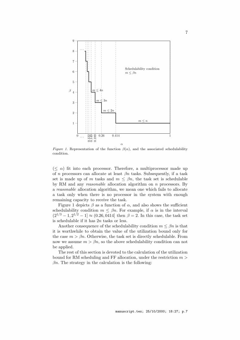
Figure 1. Representation of the function β(α), and the associated schedulabilitycondition.

(≤ α) fit into each processor. Therefore, a multiprocessor made upof n processors can allocate at least βn tasks. Subsequently, if a taskset is made up of m tasks and m ≤ βn, the task set is schedulableby RM and any reasonable allocation algorithm on n processors. Bya reasonable allocation algorithm, we mean one which fails to allocatea task only when there is no processor in the system with enoughremaining capacity to receive the task.

Figure 1 depicts β as a function of α, and also shows the sufficientschedulability condition m ≤ βn. For example, if α is in the interval(21/3 − 1, 21/2 − 1] ≈ (0.26, 0414] then β = 2. In this case, the task setis schedulable if it has 2n tasks or less.

Another consequence of the schedulability condition m ≤ βn is thatit is worthwhile to obtain the value of the utilization bound only forthe case m > βn. Otherwise, the task set is directly schedulable. Fromnow we assume m > βn, so the above schedulability condition can notbe applied.

The rest of this section is devoted to the calculation of the utilizationbound for RM scheduling and FF allocation, under the restriction m >βn. The strategy in the calculation is the following:

manuscript.tex; 25/10/2000; 18:27; p.7

8

1. Some mathematical relationships used in the proofs are presented.

2. Theorem 1 gives an upper limit on the utilization bound.

3. Lemma 3 is proved. This lemma is necessary in order to proveTheorem 2.

4. Theorem 2 proves an expression which relates the utilization boundfor m tasks and n processors, with the utilization bound for (m−β)tasks and (n − 1) processors.

5. From the result given in step 4, and Liu & Layland’s bound foruniprocessors, Theorem 3 obtains a lower limit on the utilizationbound. The upper and lower limits on the utilization bound givenin steps 2 and 5 are the same. Finally, Theorem 3 gives the exactvalue of the utilization bound, which coincides with the upper andlower limits.

Before calculating URM-FFwc (m,n, α), some relationships of the positive

integer numbers, Z+, are presented without proof.

(i) x + 1 ≤ y ∀x, y ∈ Z+ | x < y

(ii) (21/x − 1)x > (21/y − 1)y > ln 2 ∀x, y ∈ Z+ | x < y

(iii) (21/(x+1) − 1)x < (21/(y+1) − 1)y < ln 2 ∀x, y ∈ Z+ | x < y

These will be referred to as Relationship (i), Relationship (ii), andRelationship (iii).

The following theorem gives an upper limit on the utilization boundusing RM scheduling and FF allocation. The proof is based on findinga task set which does not fit into the processors.

THEOREM 1. If m > βn then

URM-FF

wc (m,n, α) ≤ (n − 1)(21/(β+1) − 1)β

+ (m − β(n − 1))(21/(m−β(n−1)) − 1)(7)

Proof. Let us define

g(m,n, α) = (n − 1)(21/(β+1) − 1)β

+ (m − β(n − 1))(21/(m−β(n−1)) − 1)

We will prove that there exists a set of m tasks, {τ1, . . . , τm}, withutilization factors 0 < ui ≤ α for all i = 1, . . . ,m, and total utilizationU = g(m,n, α) + ǫ, given ǫ → 0+, which does not fit into n processors,using FF allocation and Liu & Layland’s bound for RM scheduling.

manuscript.tex; 25/10/2000; 18:27; p.8

9

This set of m tasks is made up of two subsets: a first subset with(m − βn) tasks, and a second subset with βn tasks.

All the tasks of the first subset have the same utilization factor ofvalue

ui =(m − β(n − 1))(21/(m−β(n−1)) − 1) − (21/(β+1) − 1)β

(m − βn)(8)

where i = 1, . . . , (m − βn).All the tasks of the second subset have the same utilization factor

of valueui = (21/(β+1) − 1) +

ǫ

βn

where i = (m − βn + 1), . . . ,m.It can be easily checked that the total utilization of the whole task

set is g(m,n, α) + ǫ.Firstly, it is necessary to prove that the utilization factors of both

subsets are valid, i.e, 0 < ui ≤ α for all i = 1, . . . ,m.Check of the utilization factors of the first subset.

By hypothesis, m > βn, so m − β(n − 1) > β. Applying Relation-ship (i) we get m − β(n − 1) ≥ β + 1. Now applying Relationship (ii)makes (m − β(n − 1))(21/(m−β(n−1)) − 1) ≤ (β + 1)(21/(β+1) − 1).Considering this expression and equation (8) we get

ui ≤(21/(β+1) − 1)

(m − βn)(9)

On one hand, Lemma 2 provides the value β = ⌊1/ log2(α + 1)⌋.Thus, (β + 1) > 1/ log2(α + 1), and finding α

α > (21/(β+1) − 1) (10)

On the other hand m > βn by hypothesis, so (m − βn) > 0, andapplying Relationship (i) we get

m − βn ≥ 1 (11)

Substituting (10), and (11) into (9) proves that ui < α for all thetasks of the first subset.

Next we will prove that all the utilization factors of the first subsetare greater than zero. From Relationships (ii), (iii), and equation (11)we get

(m − β(n − 1))(21/(m−β(n−1)) − 1) > ln 2

(21/(β+1) − 1)β < ln 2

m − βn ≥ 1

manuscript.tex; 25/10/2000; 18:27; p.9

10

Substituting the above expressions into equation (8) gives ui > 0 forall the tasks of the first subset.

Check of the utilization factors of the second subset.

It is always possible to find one real number between two real num-bers. Hence, from equation (10), a positive value ǫ/(βn) must exist suchthat

α > (21/(β+1) − 1) +ǫ

βn= ui (12)

which proves that the utilization factors of the second subset are lessthan α when ǫ → 0+. In addition, the utilization factors of the secondsubset are obviously greater than zero.

From the above results, we conclude that the proposed task set isvalid. Next we prove that it does not fit into n processors, using Liu &Layland’s bound for RM scheduling and FF allocation.

The first subset of tasks, {τ1, . . . , τm−βn}, and the first β tasks ofthe second subset, {τm−βn+1, . . . , τm−βn+β}, do not fit into processorP1, since the total utilization of these tasks is over Liu & Layland’sbound.

m−βn+β∑

i=1

ui =m−βn∑

i=1

ui +m−βn+β

∑

i=m−βn+1

ui

= (m − β(n − 1))(21/(m−β(n−1)) − 1) +ǫ

n

> (m − β(n − 1))(21/(m−β(n−1)) − 1)

However, from the above expression it can be proved that if taskτm−βn+β is removed, then the first subset of tasks, and the first (β−1)tasks of the second subset do fit into processor P1.

Hence, there are β(n−1)+1 tasks left of utilization factor, (21/(β+1)−1) + ǫ

βn , which FF tries to allocate to the last (n − 1) processors,

{P2, . . . , Pn}.No processor in the set {P2, . . . , Pn} can allocate (β + 1) or more

tasks of the second subset, since (β + 1) of these tasks together have autilization over Liu & Layland’s bound.

(β + 1)

(

(21/(β+1) − 1) +ǫ

βn

)

> (β + 1)(21/(β+1) − 1)

However, each processor in {P2, . . . , Pn} can allocate β tasks, as bythe definition of β, at least β tasks can be allocated to each processor.

Subsequently, tasks {τm−βn+β , . . . , τm−1} are allocated to proces-sors, but the last one, τm, can not be allocated to any processor.

manuscript.tex; 25/10/2000; 18:27; p.10

11

We conclude that the proposed task set of total utilization g(m,n, α)+ǫ does not fit into n processors when ǫ → 0+, so the utilization bound,URM-FF

wc (m,n, α), must be less than or equal to g(m,n, α). �The proof of Theorem 2 requires Lemma 3, which is proved below.

It relates the utilization bound for the same number of processors, buta different number of tasks.

LEMMA 3.

URM-FF

wc (q, n, α) ≥ URM-FF

wc (m,n, α) for all q < m

Proof. This lemma will be proved by contradiction.Let us suppose that a pair of integers q and m exist, such that q < m,

and URM-FFwc (q, n, α) < URM-FF

wc (m,n, α). Between two real numbers, itis always possible to find another real number, so we can find an ǫ > 0such that

URM-FFwc (q, n, α) < URM-FF

wc (m,n, α) − ǫ < URM-FFwc (m,n, α)

By the definition of utilization bound, there exists at least one setof q tasks, {τ1, . . . , τq}, of total utilization

q∑

i=1

ui = URM-FFwc (m,n, α) − ǫ

which does not fit into n processors. Next, we prove that this gives riseto a contradiction.

If we add to this task set (m − q) new tasks, {τq+1, . . . , τm}, eachof utilization factor ǫ/(m − q), we obtain a task set made up of mtasks of total utilization

∑mi=1 ui = URM-FF

wc (m,n, α), which fits inton processors. Hence, the first q tasks fit into n processors, which is acontradiction. �

Next, we prove an expression which relates the utilization boundof multiprocessors with n and (n − 1) processors. This will allow us toobtain a lower limit for the utilization bound, going from the case n = 1(uniprocessor case) to a general multiprocessor case with an arbitraryn.

THEOREM 2. If m > βn then

URM-FF

wc (m,n, α) ≥ (21/(β+1) − 1)β + URM-FF

wc (m − β, n − 1, α)

manuscript.tex; 25/10/2000; 18:27; p.11

12

τ1 · · · τk−1 τk τk+1 · · · τm−β · · · τm

URM-FFwc (m − β, n − 1, α) ∆

uk,1

u1 uk−1 uk uk+1 um−β um

m∑

i=k

ui

m−β∑

i=1

ui

k−1∑

i=1

ui

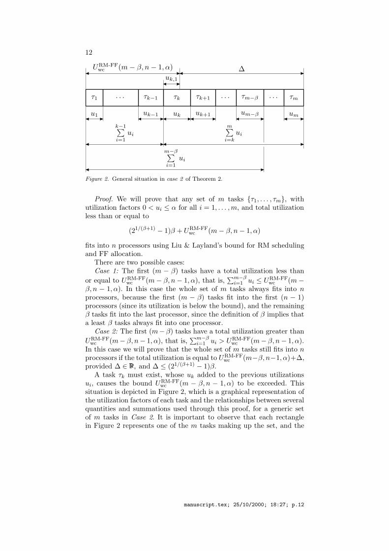
Figure 2. General situation in case 2 of Theorem 2.

Proof. We will prove that any set of m tasks {τ1, . . . , τm}, withutilization factors 0 < ui ≤ α for all i = 1, . . . ,m, and total utilizationless than or equal to

(21/(β+1) − 1)β + URM-FFwc (m − β, n − 1, α)

fits into n processors using Liu & Layland’s bound for RM schedulingand FF allocation.

There are two possible cases:Case 1: The first (m − β) tasks have a total utilization less than

or equal to URM-FFwc (m − β, n − 1, α), that is,

∑m−βi=1 ui ≤ URM-FF

wc (m −β, n − 1, α). In this case the whole set of m tasks always fits into nprocessors, because the first (m − β) tasks fit into the first (n − 1)processors (since its utilization is below the bound), and the remainingβ tasks fit into the last processor, since the definition of β implies thata least β tasks always fit into one processor.

Case 2: The first (m−β) tasks have a total utilization greater than

URM-FFwc (m− β, n− 1, α), that is,

∑m−βi=1 ui > URM-FF

wc (m− β, n− 1, α).In this case we will prove that the whole set of m tasks still fits into nprocessors if the total utilization is equal to URM-FF

wc (m−β, n−1, α)+∆,provided ∆ ∈ R, and ∆ ≤ (21/(β+1) − 1)β.

A task τk must exist, whose uk added to the previous utilizationsui, causes the bound URM-FF

wc (m − β, n − 1, α) to be exceeded. Thissituation is depicted in Figure 2, which is a graphical representation ofthe utilization factors of each task and the relationships between severalquantities and summations used through this proof, for a generic setof m tasks in Case 2. It is important to observe that each rectanglein Figure 2 represents one of the m tasks making up the set, and the

manuscript.tex; 25/10/2000; 18:27; p.12

13

horizontal dimension of each rectangle gives the utilization factor ofthe task it represents.

The value of k is obtained as the integer which fulfills:

k−1∑

i=1

ui ≤ URM-FFwc (m − β, n − 1, α) <

k∑

i=1

ui

Note that k ≤ m − β (if k > m − β we would be in case 1).It can be seen that the first (k − 1) tasks fit into the first (n − 1)

processors. The total utilization of the first (k − 1) tasks fulfills

k−1∑

i=1

ui ≤ URM-FFwc (m − β, n − 1, α)

Bearing in mind that k− 1 < m−β in Case 2, and applying Lemma 3,we get

URM-FFwc (m − β, n − 1, α) ≤ URM-FF

wc (k − 1, n − 1, α)

and thusk−1∑

i=1

ui ≤ URM-FFwc (k − 1, n − 1, α)

Therefore, the first (k − 1) tasks fit into the first (n− 1) processors.We only have to prove that the remaining (m− k +1) tasks fit into thelast processor.

The worst situation in terms of schedulability appears when all thetasks τi in {τk, . . . , τm} fulfill ui > uk,1, where

uk,1 = URM-FFwc (m − β, n − 1, α) −

k−1∑

i=1

ui

as shown in Figure 2. Note that if there were a task τi in {τk, . . . , τm}with ui ≤ uk,1, we could always allocate this task to the first (n − 1)processors (since the addition of this new task does not cause the totalutilization to exceed the bound), and the result would be a situationanalogous to the current one, with k one unit greater. This reasoningcan be repeated until no task τi with ui ≤ uk,1 exists among the last(m − k + 1) tasks, or until we are in Case 1.

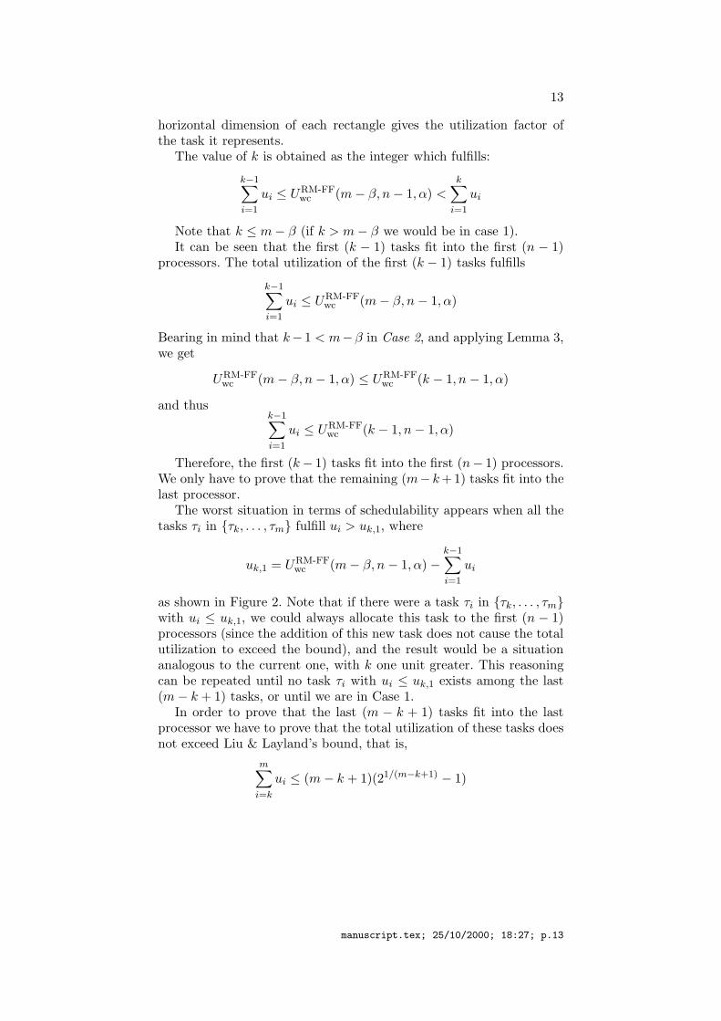
In order to prove that the last (m − k + 1) tasks fit into the lastprocessor we have to prove that the total utilization of these tasks doesnot exceed Liu & Layland’s bound, that is,

m∑

i=k

ui ≤ (m − k + 1)(21/(m−k+1) − 1)

manuscript.tex; 25/10/2000; 18:27; p.13

14

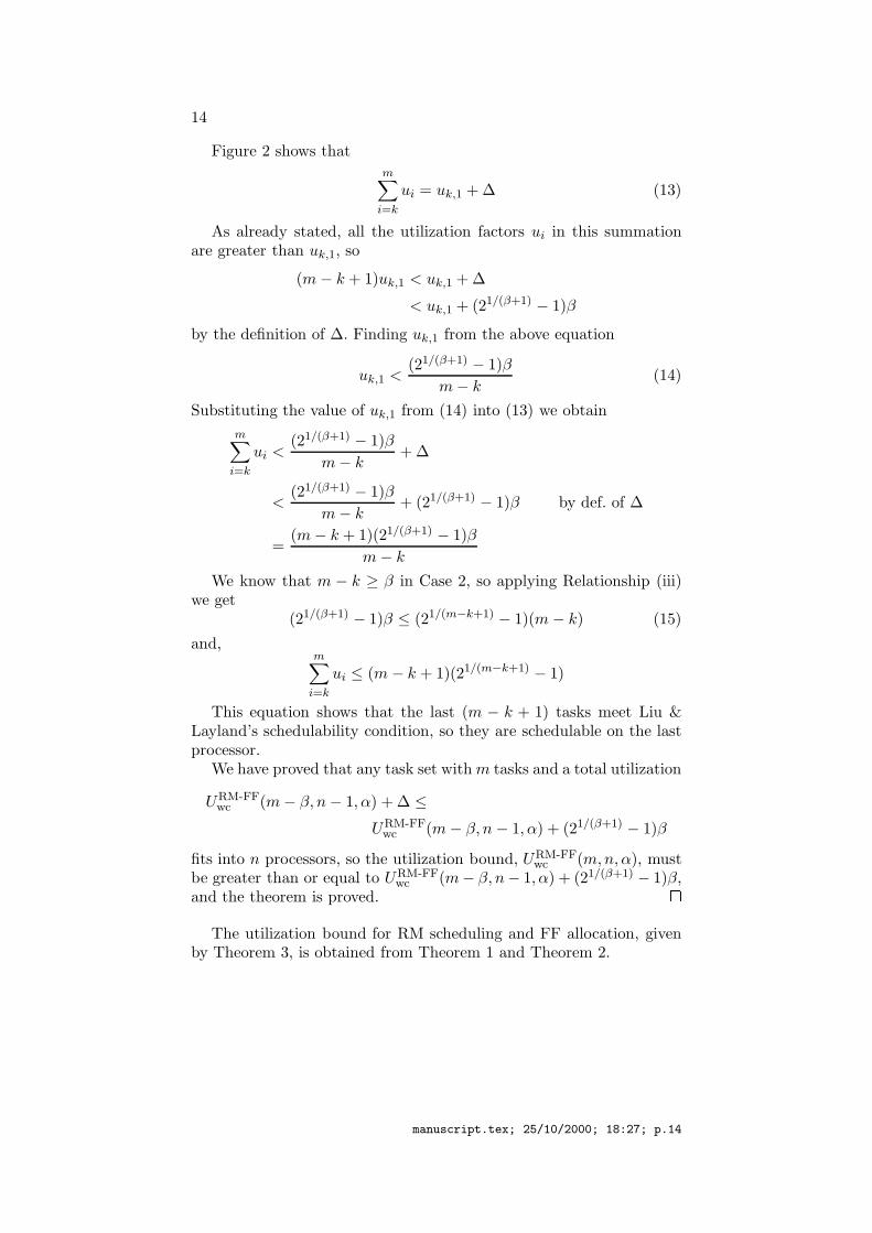
Figure 2 shows that

m∑

i=k

ui = uk,1 + ∆ (13)

As already stated, all the utilization factors ui in this summationare greater than uk,1, so

(m − k + 1)uk,1 < uk,1 + ∆

< uk,1 + (21/(β+1) − 1)β

by the definition of ∆. Finding uk,1 from the above equation

uk,1 <(21/(β+1) − 1)β

m − k(14)

Substituting the value of uk,1 from (14) into (13) we obtain

m∑

i=k

ui <(21/(β+1) − 1)β

m − k+ ∆

<(21/(β+1) − 1)β

m − k+ (21/(β+1) − 1)β by def. of ∆

=(m − k + 1)(21/(β+1) − 1)β

m − k

We know that m − k ≥ β in Case 2, so applying Relationship (iii)we get

(21/(β+1) − 1)β ≤ (21/(m−k+1) − 1)(m − k) (15)

and,m

∑

i=k

ui ≤ (m − k + 1)(21/(m−k+1) − 1)

This equation shows that the last (m − k + 1) tasks meet Liu &Layland’s schedulability condition, so they are schedulable on the lastprocessor.

We have proved that any task set with m tasks and a total utilization

URM-FFwc (m − β, n − 1, α) + ∆ ≤

URM-FFwc (m − β, n − 1, α) + (21/(β+1) − 1)β

fits into n processors, so the utilization bound, URM-FFwc (m,n, α), must

be greater than or equal to URM-FFwc (m− β, n− 1, α) + (21/(β+1) − 1)β,

and the theorem is proved. �The utilization bound for RM scheduling and FF allocation, given

by Theorem 3, is obtained from Theorem 1 and Theorem 2.

manuscript.tex; 25/10/2000; 18:27; p.14

15

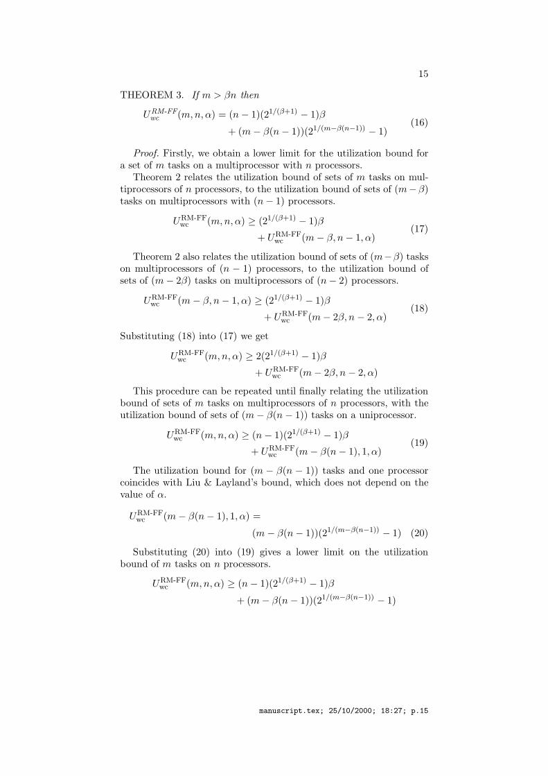
THEOREM 3. If m > βn then

URM-FF

wc (m,n, α) = (n − 1)(21/(β+1) − 1)β

+ (m − β(n − 1))(21/(m−β(n−1)) − 1)(16)

Proof. Firstly, we obtain a lower limit for the utilization bound fora set of m tasks on a multiprocessor with n processors.

Theorem 2 relates the utilization bound of sets of m tasks on mul-tiprocessors of n processors, to the utilization bound of sets of (m−β)tasks on multiprocessors with (n − 1) processors.

URM-FFwc (m,n, α) ≥ (21/(β+1) − 1)β

+ URM-FFwc (m − β, n − 1, α)

(17)

Theorem 2 also relates the utilization bound of sets of (m−β) taskson multiprocessors of (n − 1) processors, to the utilization bound ofsets of (m − 2β) tasks on multiprocessors of (n − 2) processors.

URM-FFwc (m − β, n − 1, α) ≥ (21/(β+1) − 1)β

+ URM-FFwc (m − 2β, n − 2, α)

(18)

Substituting (18) into (17) we get

URM-FFwc (m,n, α) ≥ 2(21/(β+1) − 1)β

+ URM-FFwc (m − 2β, n − 2, α)

This procedure can be repeated until finally relating the utilizationbound of sets of m tasks on multiprocessors of n processors, with theutilization bound of sets of (m − β(n − 1)) tasks on a uniprocessor.

URM-FFwc (m,n, α) ≥ (n − 1)(21/(β+1) − 1)β

+ URM-FFwc (m − β(n − 1), 1, α)

(19)

The utilization bound for (m − β(n − 1)) tasks and one processorcoincides with Liu & Layland’s bound, which does not depend on thevalue of α.

URM-FFwc (m − β(n − 1), 1, α) =

(m − β(n − 1))(21/(m−β(n−1)) − 1) (20)

Substituting (20) into (19) gives a lower limit on the utilizationbound of m tasks on n processors.

URM-FFwc (m,n, α) ≥ (n − 1)(21/(β+1) − 1)β

+ (m − β(n − 1))(21/(m−β(n−1)) − 1)

manuscript.tex; 25/10/2000; 18:27; p.15

16

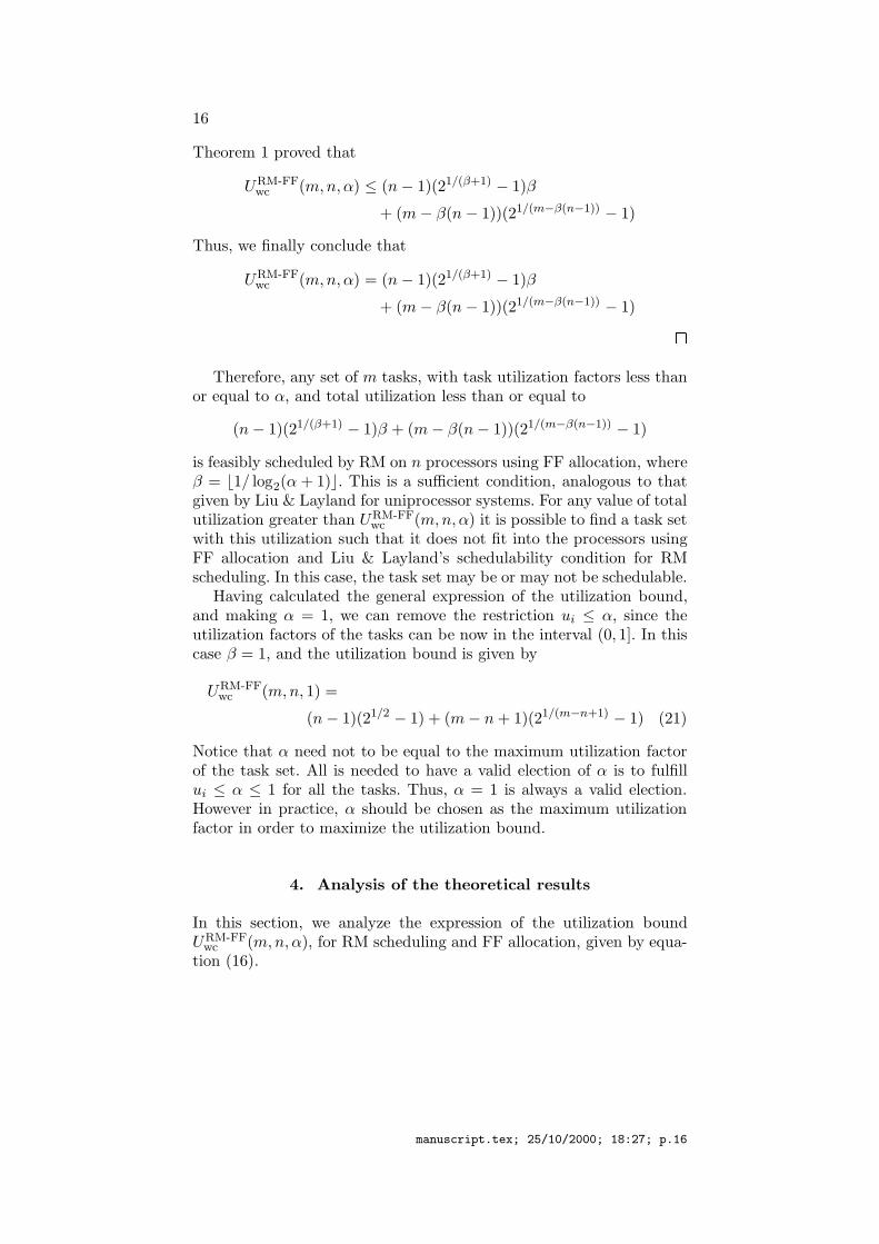
Theorem 1 proved that

URM-FFwc (m,n, α) ≤ (n − 1)(21/(β+1) − 1)β

+ (m − β(n − 1))(21/(m−β(n−1)) − 1)

Thus, we finally conclude that

URM-FFwc (m,n, α) = (n − 1)(21/(β+1) − 1)β

+ (m − β(n − 1))(21/(m−β(n−1)) − 1) �Therefore, any set of m tasks, with task utilization factors less than

or equal to α, and total utilization less than or equal to

(n − 1)(21/(β+1) − 1)β + (m − β(n − 1))(21/(m−β(n−1)) − 1)

is feasibly scheduled by RM on n processors using FF allocation, whereβ = ⌊1/ log2(α + 1)⌋. This is a sufficient condition, analogous to thatgiven by Liu & Layland for uniprocessor systems. For any value of totalutilization greater than URM-FF

wc (m,n, α) it is possible to find a task setwith this utilization such that it does not fit into the processors usingFF allocation and Liu & Layland’s schedulability condition for RMscheduling. In this case, the task set may be or may not be schedulable.

Having calculated the general expression of the utilization bound,and making α = 1, we can remove the restriction ui ≤ α, since theutilization factors of the tasks can be now in the interval (0, 1]. In thiscase β = 1, and the utilization bound is given by

URM-FFwc (m,n, 1) =

(n − 1)(21/2 − 1) + (m − n + 1)(21/(m−n+1) − 1) (21)

Notice that α need not to be equal to the maximum utilization factorof the task set. All is needed to have a valid election of α is to fulfillui ≤ α ≤ 1 for all the tasks. Thus, α = 1 is always a valid election.However in practice, α should be chosen as the maximum utilizationfactor in order to maximize the utilization bound.

4. Analysis of the theoretical results

In this section, we analyze the expression of the utilization boundURM-FF

wc (m,n, α), for RM scheduling and FF allocation, given by equa-tion (16).

manuscript.tex; 25/10/2000; 18:27; p.16

17

0

1

2

3

3.5

ln 2 →

0 5 10 15 20 25

n = 1

n = 2

n = 3

n = 4

n = 5

21/2 − 1

Number of processors (n)

Number of tasks (m)

URM-FFwc (m,n, 1)

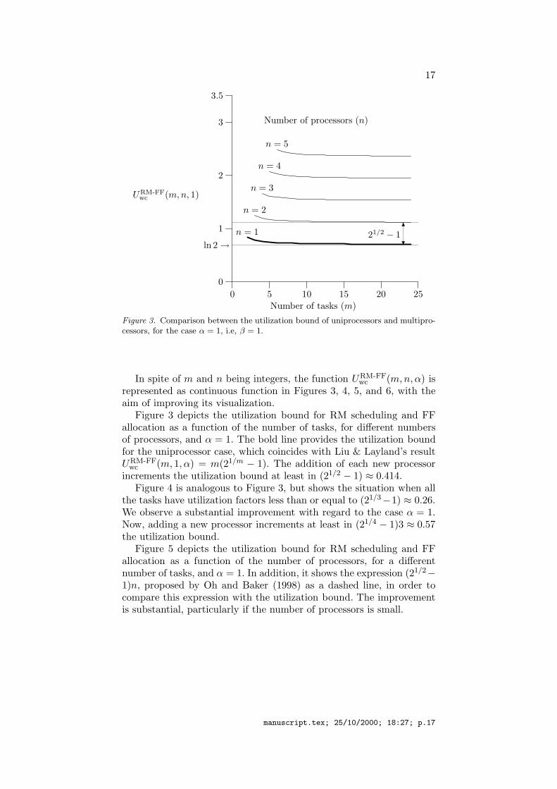
Figure 3. Comparison between the utilization bound of uniprocessors and multipro-cessors, for the case α = 1, i.e, β = 1.

In spite of m and n being integers, the function URM-FFwc (m,n, α) is

represented as continuous function in Figures 3, 4, 5, and 6, with theaim of improving its visualization.

Figure 3 depicts the utilization bound for RM scheduling and FFallocation as a function of the number of tasks, for different numbersof processors, and α = 1. The bold line provides the utilization boundfor the uniprocessor case, which coincides with Liu & Layland’s resultURM-FF

wc (m, 1, α) = m(21/m − 1). The addition of each new processorincrements the utilization bound at least in (21/2 − 1) ≈ 0.414.

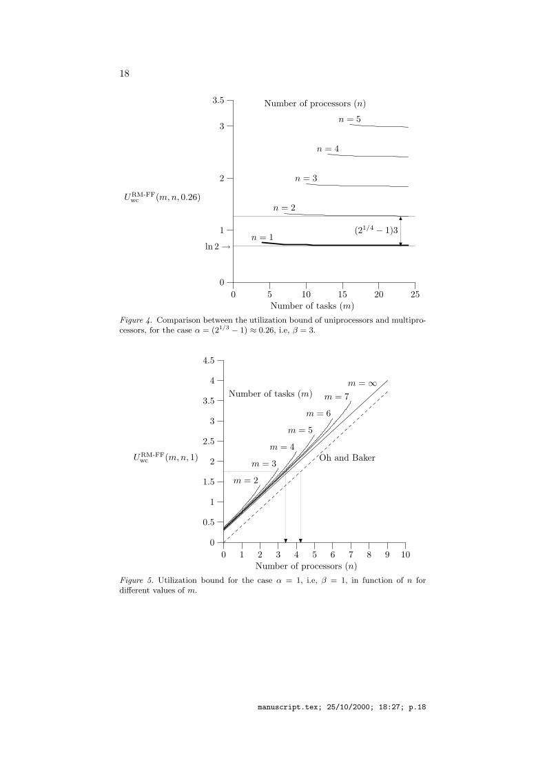
Figure 4 is analogous to Figure 3, but shows the situation when allthe tasks have utilization factors less than or equal to (21/3−1) ≈ 0.26.We observe a substantial improvement with regard to the case α = 1.Now, adding a new processor increments at least in (21/4 − 1)3 ≈ 0.57the utilization bound.

Figure 5 depicts the utilization bound for RM scheduling and FFallocation as a function of the number of processors, for a differentnumber of tasks, and α = 1. In addition, it shows the expression (21/2−1)n, proposed by Oh and Baker (1998) as a dashed line, in order tocompare this expression with the utilization bound. The improvementis substantial, particularly if the number of processors is small.

manuscript.tex; 25/10/2000; 18:27; p.17

18

0

1

2

3

3.5

ln 2 →

0 5 10 15 20 25

n = 1

n = 2

n = 3

n = 4

n = 5

(21/4 − 1)3

Number of processors (n)

Number of tasks (m)

URM-FFwc (m,n, 0.26)

Figure 4. Comparison between the utilization bound of uniprocessors and multipro-cessors, for the case α = (21/3 − 1) ≈ 0.26, i.e, β = 3.

0

0.5

1

1.5

2

2.5

3

3.5

4

4.5

0 1 2 3 4 5 6 7 8 9 10

m = 2

m = 3

m = 4

m = 5

m = 6

m = 7

m = ∞Number of tasks (m)

Oh and Baker

Number of processors (n)

URM-FFwc (m,n, 1)

Figure 5. Utilization bound for the case α = 1, i.e, β = 1, in function of n fordifferent values of m.

manuscript.tex; 25/10/2000; 18:27; p.18

19

0

0.5

1

1.5

2

2.5

0 1 2 3 4

m = 2

m = 3

m = 4

m = 5

m = 6

m = 7

m = ∞

Number of tasks (m)

Oh and Baker

Number of processors (n)

URM-FFwc (m,n, 0.26)

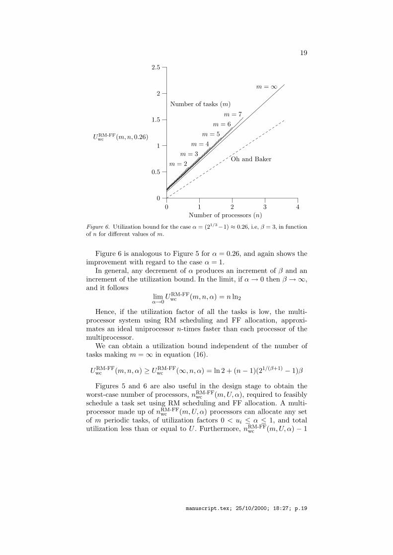
Figure 6. Utilization bound for the case α = (21/3−1) ≈ 0.26, i.e, β = 3, in functionof n for different values of m.

Figure 6 is analogous to Figure 5 for α = 0.26, and again shows theimprovement with regard to the case α = 1.

In general, any decrement of α produces an increment of β and anincrement of the utilization bound. In the limit, if α → 0 then β → ∞,and it follows

limα→0

URM-FFwc (m,n, α) = n ln2

Hence, if the utilization factor of all the tasks is low, the multi-processor system using RM scheduling and FF allocation, approxi-mates an ideal uniprocessor n-times faster than each processor of themultiprocessor.

We can obtain a utilization bound independent of the number oftasks making m = ∞ in equation (16).

URM-FFwc (m,n, α) ≥ URM-FF

wc (∞, n, α) = ln 2 + (n − 1)(21/(β+1) − 1)β

Figures 5 and 6 are also useful in the design stage to obtain theworst-case number of processors, nRM-FF

wc (m,U,α), required to feasiblyschedule a task set using RM scheduling and FF allocation. A multi-processor made up of nRM-FF

wc (m,U,α) processors can allocate any setof m periodic tasks, of utilization factors 0 < ui ≤ α ≤ 1, and totalutilization less than or equal to U . Furthermore, nRM-FF

wc (m,U,α) − 1

manuscript.tex; 25/10/2000; 18:27; p.19

20

processors may not be enough, and it is possible to find at least oneset of m periodic tasks, of utilization factors 0 < ui ≤ α ≤ 1, and totalutilization less than or equal to U , which can not be allocated.

For example, consider a task set made up of m = 7 tasks, of totalutilization U = 1.75, and arbitrary utilization factors. From Figure 5,applying the expression proposed by Oh and Baker (1998) five proces-sors are needed. However, applying the utilization bound presented inthis paper, we only need nRM-FF

wc (7, 1.75, 1) = 4 processors. If we usethree processors it is possible to find a set of seven tasks which is notschedulable by RM and FF. For instance, the task set with utilizationfactors {u1 = 0.01, u2 = 0.01, u3 = 0.01, u4 = 0.43, u5 = 0.43, u6 =0.43, u7 = 0.43} does not fit into three processors.

Figures 5 and 6 are only valid for m > βn. Therefore, if there is nota point in these figures for some pair of values (m,U), the worst-casenumber of processors is obtained as the minimum integer value greaterthan or equal to m/β.

nRM-FFwc (m,U,α) =

⌈

m

β

⌉

(22)

For example, for m = 3, U = 2.5, and β = 1, there is not a point inFigure 5, and so nRM-FF

wc (3, 2.5, 1) = ⌈3/1⌉ = 3 processors.

5. Average-case behaviour

Section 3 provided the utilization bound for RM scheduling and FFallocation. Any task set of total utilization less than or equal to theutilization bound is schedulable. In addition, for any given value of totalutilization greater than the utilization bound, task sets which do not fitinto the processors using Liu & Layland’s schedulability condition andFF allocation exist. However, tasks sets of total utilization greater thanthe utilization bound may be schedulable. In fact, the utilization boundis obtained for pessimistic task sets which might be very infrequent inpractice.

In order to perceive the pessimism of the utilization bound, wewill define the average-case utilization bound, URM-FF

ac (m,n, p), for RMscheduling and FF allocation as follows.

DEFINITION 2. A task set made up of m tasks, of total utilization

U = URM-FFac (m,n, p) is schedulable by RM and FF on n processors

with a probability equal to p%.

If sets of m tasks with total utilization U = URM-FFac (m,n, p) are

randomly generated, p% of the task sets are schedulable by RM and

manuscript.tex; 25/10/2000; 18:27; p.20

21

FF on n processors. The other (100−p)% corresponds to task sets whichdo not fit into the processors. Obviously, the average-case utilizationbound must be greater than or equal to the (worst-case) utilizationbound.

URM-FFac (m,n, p) ≥ URM-FF

wc (m,n, α = 1)

The equality corresponds to the case p = 100%.

URM-FFac (m,n, p = 100%) = URM-FF

wc (m,n, α = 1)

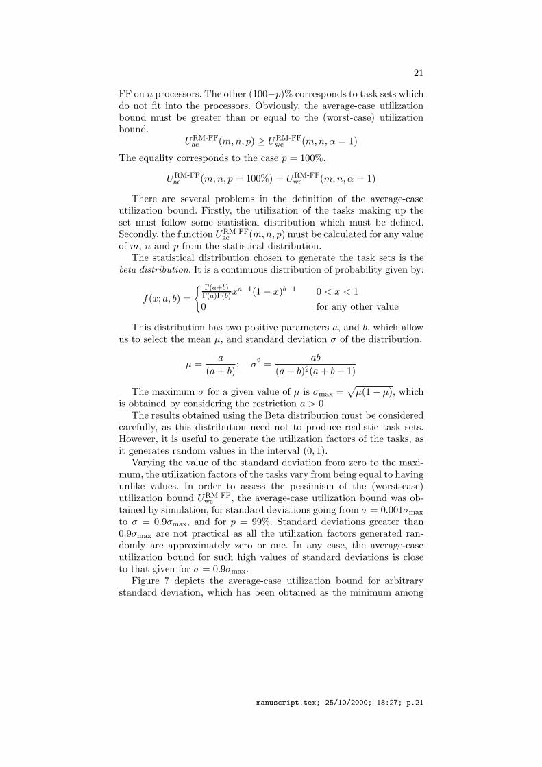
There are several problems in the definition of the average-caseutilization bound. Firstly, the utilization of the tasks making up theset must follow some statistical distribution which must be defined.Secondly, the function URM-FF

ac (m,n, p) must be calculated for any valueof m, n and p from the statistical distribution.

The statistical distribution chosen to generate the task sets is thebeta distribution. It is a continuous distribution of probability given by:

f(x; a, b) =

{

Γ(a+b)Γ(a)Γ(b)x

a−1(1 − x)b−1 0 < x < 1

0 for any other value

This distribution has two positive parameters a, and b, which allowus to select the mean µ, and standard deviation σ of the distribution.

µ =a

(a + b); σ2 =

ab

(a + b)2(a + b + 1)

The maximum σ for a given value of µ is σmax =√

µ(1 − µ), whichis obtained by considering the restriction a > 0.

The results obtained using the Beta distribution must be consideredcarefully, as this distribution need not to produce realistic task sets.However, it is useful to generate the utilization factors of the tasks, asit generates random values in the interval (0, 1).

Varying the value of the standard deviation from zero to the maxi-mum, the utilization factors of the tasks vary from being equal to havingunlike values. In order to assess the pessimism of the (worst-case)utilization bound URM-FF

wc , the average-case utilization bound was ob-tained by simulation, for standard deviations going from σ = 0.001σmax

to σ = 0.9σmax, and for p = 99%. Standard deviations greater than0.9σmax are not practical as all the utilization factors generated ran-domly are approximately zero or one. In any case, the average-caseutilization bound for such high values of standard deviations is closeto that given for σ = 0.9σmax.

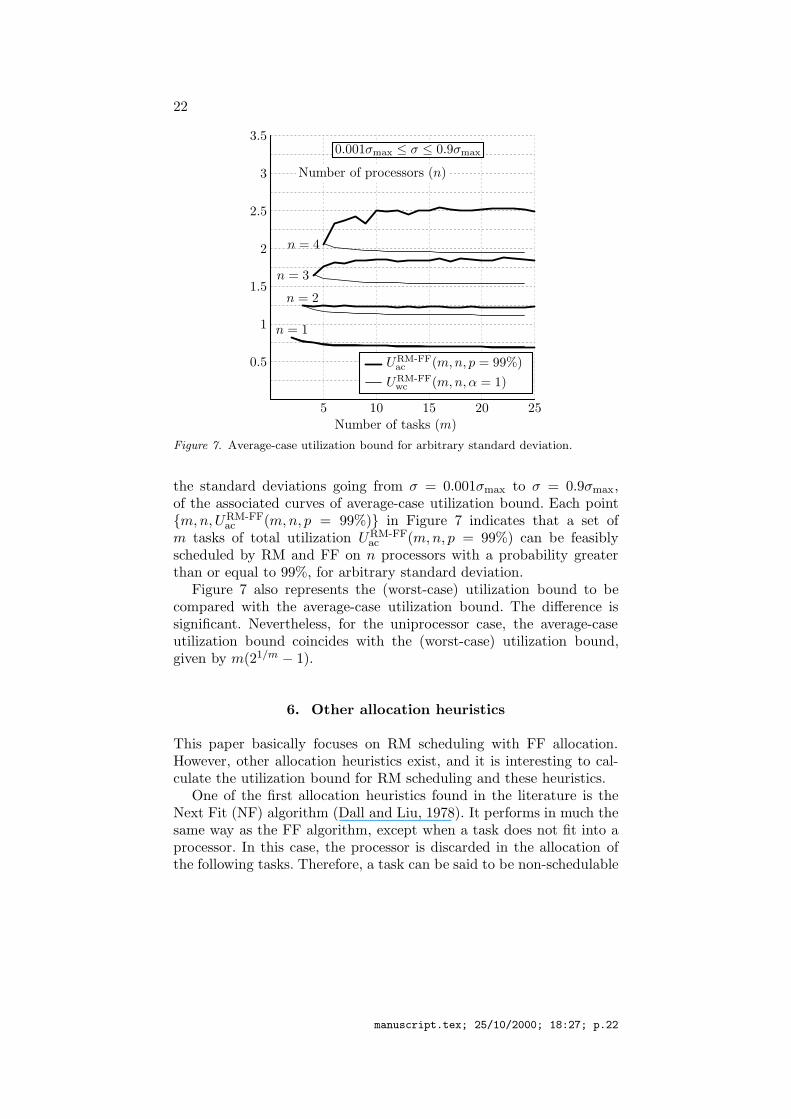
Figure 7 depicts the average-case utilization bound for arbitrarystandard deviation, which has been obtained as the minimum among

manuscript.tex; 25/10/2000; 18:27; p.21

22

0.5

1

1.5

2

2.5

3

3.5

5 10 15 20 25

n = 1

n = 2

n = 3

n = 4

0.001σmax ≤ σ ≤ 0.9σmax

Number of processors (n)

URM-FFac (m,n, p = 99%)

URM-FFwc (m,n, α = 1)

Number of tasks (m)

Figure 7. Average-case utilization bound for arbitrary standard deviation.

the standard deviations going from σ = 0.001σmax to σ = 0.9σmax,of the associated curves of average-case utilization bound. Each point{m,n,URM-FF

ac (m,n, p = 99%)} in Figure 7 indicates that a set ofm tasks of total utilization URM-FF

ac (m,n, p = 99%) can be feasiblyscheduled by RM and FF on n processors with a probability greaterthan or equal to 99%, for arbitrary standard deviation.

Figure 7 also represents the (worst-case) utilization bound to becompared with the average-case utilization bound. The difference issignificant. Nevertheless, for the uniprocessor case, the average-caseutilization bound coincides with the (worst-case) utilization bound,given by m(21/m − 1).

6. Other allocation heuristics

This paper basically focuses on RM scheduling with FF allocation.However, other allocation heuristics exist, and it is interesting to cal-culate the utilization bound for RM scheduling and these heuristics.

One of the first allocation heuristics found in the literature is theNext Fit (NF) algorithm (Dall and Liu, 1978). It performs in much thesame way as the FF algorithm, except when a task does not fit into aprocessor. In this case, the processor is discarded in the allocation ofthe following tasks. Therefore, a task can be said to be non-schedulable

manuscript.tex; 25/10/2000; 18:27; p.22

23

even when it fits in one of the discarded processors. As a result, theNF algorithm presents poor performance with regard to the FF al-gorithm, which is expressed in terms of the metric (NNF/Nopt). Dalland Liu (1978) obtained (NNF/Nopt) = 2.67, compared with the value(NFF/Nopt) = 2.33, obtained by Oh and Son (1995) for FF allocation.

Another common algorithm found in the literature is the Best Fit(BF) (Garey and Johnson, 1979). This algorithm assigns each task tothe processor having the lowest remaining capacity among those pro-cessors with enough capacity. Intuitively, BF seems to be an improve-ment over the FF algorithm, so it should provide better performance.However, simulation experiments carried out by the authors with BFallocation gave almost identical results to those using FF allocation, sothey have not been depicted. In addition, the utilization bound associ-ated to RM scheduling with BF allocation is the same as that for FFallocation. The proof is analogous to that presented for FF allocation,so for the sake of brevity, we provide only the guidelines . The task setused in theorem 1 (to prove the upper limit on the utilization boundfor RM-FF) does not fit into the processors using BF allocation, sothe upper limit is also valid for BF allocation. Theorem 2 is also validfor RM-BF, but proving the statement “the worst situation in termsof schedulability appears when all the tasks τi in {τk, . . . , τm} fulfillui > uk,1”, requires some elaboration for BF allocation. Therefore, theutilization bound for BF allocation coincides with the upper and lowerlimits, an it is equal to the utilization bound for FF allocation.

Better approximation algorithms can be obtained by observing thatthe worst performance for both FF and BF occurs when tasks with lowutilization factors appear before tasks greater utilization factors. Thisis the case of the task set used in theorem 1 to obtain the upper limit onthe utilization bound. To improve the performance of the FF and BFalgorithms, the tasks with the lowest utilization factors are allocatedfirst. The resulting algorithms are called First Fit Decreasing (FFD)and Best Fit Decreasing (BFD) respectively.

The utilization bound for FFD or BFD can not be lower than that forFF or BF respectively. This can be proved with the following argument.Let S be the superset made up of all the task sets which do not fit intothe processors using FF allocation. There must be a task set in S,whose total utilization is the minimum among all the task sets in S.The value obtained by subtracting an ǫ → 0 from this minimum is theutilization bound for RM-FF. Let S ′ be the superset made up of all thetask sets ordered in decreasing utilization factors, which do not fit intothe processors using FF allocation. There must exist a task set in S ′,whose total utilization is the minimum among all the task sets in S ′.The value obtained by subtracting an ǫ → 0 from this minimum is the

manuscript.tex; 25/10/2000; 18:27; p.23

24

utilization bound for RM-FFD. Since S ′ is a subset of S, its minimumcan not be lower than the minimum of S, and so the utilization boundfor RM-FFD can not be lower than the utilization bound for RM-FFD.The same argument can be applied to BF and BFD allocations.

In addition, the task set proposed in theorem 1 does fit into theprocessors using FFD or BFD allocation. Thus, the utilization boundfor FFD and BFD allocation may be greater than that for FF andBF allocation. Nevertheless, further investigation into this last part isrequired.

7. Conclusions and future work

Liu & Layland’s schedulability bound for RM scheduling on multi-processors has been extended to multiprocessors under a partitioningstrategy and FF allocation. This bound is a function of the number oftasks, number of processors, and maximum reachable utilization factorof the task set. For the case of tasks with low utilization factors theutilization bound is significantly raised, reaching asymptotically thevalue n ln 2 when all the utilization factors are close to zero. Allowing alow percentage of non-schedulable task sets, simulation has shown thepessimism of the utilization bound.

In general, the calculation of utilization bounds is a problem of im-portance in the real-time theory. Utilization bounds allow us not onlyto perform fast schedulability tests, but also to perform a schedulabilityanalysis. That is, utilization bounds allow us to establish the influenceof different parameters such as the number of tasks, task size, etc,on the schedulability of the system by considering the worst-case. Inaddition, utilization bounds indicate how far the system is from theideal situation, in which, the total utilization equals the number ofprocessors in the system.

Other allocation heuristics apart from FF have been dealt withbriefly. The NF algorithm was shown to have worse performance thanthe FF algorithm. Since NF presents no practical advantage over FF,NF will not be considered in future works.

Simulation results have shown a behaviour of BF allocation almostidentical to that of FF. This behaviour was previously observed byother authors (Garey and Johnson, 1979; Oh and Son, 1995). Thesame behaviour was also documented in terms of the metric (NA/Nopt)by Oh and Son (1995). In addition, the utilization bound for RM-FFand RM-BF are the same. This point was not proved in this paper,although the guidelines of the proof were provided. The computationalcost associated to the BF allocation is in general greater that that

manuscript.tex; 25/10/2000; 18:27; p.24

25

associated to FF allocation. Thus, we can state that FF allocation issuperior to BF allocation for multiprocessor RM scheduling.

In order to improve the utilization bound for RM-FF scheduling, wehave investigated the utilization bound for FFD and BFD allocation.We suspect that it is greater, but we do not have proof of this point.The calculation of the utilization bound for the heuristics FFD andBFD will be performed in future work.

Finally, the utilization bound presented in this paper has a majorrestriction. It assumes the simple model of tasks defined by Liu &Layland. In future work, we will try to develop new utilization boundsconsidering extensions to the task model, such as access to sharedresources, aperiodic tasks, release jitter, or mode changes.

8. Acknowledgments

We would like to thank the referees. Their remarks allowed us toimprove the quality of this work.

References

Burchard, A., J. Liebeherr, Y. Oh, and S. Son: 1995, ‘New Strategies for AssigningReal-Time Tasks to Multiprocessor Systems’. IEEE Transactions on Computers

44(12).Dall, S. and C. Liu: 1978, ‘On a Real-Time Scheduling Problem’. Operations

Research 6(1), 127–140.Garey, M. and D. Johnson: 1979, Computers and Intractability, pp. 121–127. New

York: W.H. Freman.Liu, C. L. and J. Layland: 1973, ‘Scheduling Algorithms for Multiprogramming in

a Hard-Real-time Environment’. Journal of the ACM 20(1), 46–61.Oh, D. and T. Baker: 1998, ‘Utilization Bounds for N-Processor Rate Monotone

Scheduling with Static Processor Assignment’. Real-Time Systems 15(2), 183–193.

Oh, Y. and S. Son: 1995, ‘Allocating Fixed-Priority Periodic Tasks on MultiprocessorSystems’. Real-Time Systems 9(3), 207–239.

S. Saez, J. V. and A. Crespo: 1998, ‘Using Exact Feasibility Tests for Allocating Real-Time Tasks in Multiprocessor Systems’. In: Proceedings of the 10th Euromicro

Workshop on Real-Time Systems. pp. 53–60.

manuscript.tex; 25/10/2000; 18:27; p.25