a hybrid method for solving stochastic job shop scheduling problems

Applied Mathematics and Computation 170 (2005) 185–206

www.elsevier.com/locate/amc

A hybrid method for solving stochasticjob shop scheduling problems

R. Tavakkoli-Moghaddam a, F. Jolai a, F. Vaziri a,P.K. Ahmed b, A. Azaron c,*

a Department of Industrial Engineering, Faculty of Engineering, University of Tehran, Tehran, Iranb Business School, University of Wolverhampton, Shropshire, United Kingdom

c Department of Artificial Complex Systems Engineering, Graduate School of Engineering,

Hiroshima University, Kagamiyama 1-4-1, Higashi-Hiroshima, Hiroshima 739-8527, Japan

Abstract

This paper presents a nonlinear mathematical programming model for a stochastic

job shop scheduling problem. Due to the complexity of the proposed model, traditional

algorithms have low capability in producing a feasible solution. Therefore, a hybrid

method is proposed to obtain a near-optimal solution within a reasonable amount of

time. This method uses a neural network approach to generate initial feasible solutions

and then a simulated annealing algorithm to improve the quality and performance of

the initial solutions in order to produce the optimal/near-optimal solution. A number

of test problems are randomly generated to verify and validate the proposed hybrid

method. The computational results obtained by this method are compared with lower

bound solutions reported by the Lingo 6 optimization software. The compared results

of these two methods show that the proposed hybrid method is more effective when the

problem size increases.

� 2005 Elsevier Inc. All rights reserved.

0096-3003/$ - see front matter � 2005 Elsevier Inc. All rights reserved.

doi:10.1016/j.amc.2004.11.036

* Corresponding author.

E-mail addresses: [email protected] (R. Tavakkoli-Moghaddam), [email protected].

ac.jp (A. Azaron).

mailto:[email protected]

mailto:[email protected].

186 R. Tavakkoli-Moghaddam et al. / Appl. Math. Comput. 170 (2005) 185–206

Keywords: Stochastic job shop scheduling; Neural networks; Simulated annealing

1. Introduction

Scheduling problem is the allocation of resources to perform a set of activ-

ities in a period of time [1]. The job shop scheduling is one of the most typical

and complicated tasks in scheduling problems. The aim of job shop scheduling

problem is to allocate n jobs to m machines in order to optimize a special factor

[2]. Traditionally, there are three approaches for solving job shop schedulingproblems, namely priority rules, combinational optimization, and constraints

analysis [3]. Recently, scheduling systems based on intelligence knowledge have

been proposed and presented [4,5]. Job shop is a production system with the

capability of producing products with a number of jobs and different operation

times for each job. Due to different operations on a product and machine

requirements to process each step of production, it is so hard to find an efficient

scheduling solution. Traditional approaches often consider small-sized prob-

lems with deterministic parameters. The real world of industry is deterministicfree and production attributes are stochastic. Stochastic variables and con-

straints are not available in the application of traditional approaches. In this

paper, we consider stochastic parameters and present a flexible algorithm to

adjust to the real-world industry situations.

Job shop scheduling problem (JSSP) is a class of combinational optimiza-

tion problems known as NP-Hard one. The above problem is a key issue in

production management and combinational optimization. In the last three dec-

ades, many researchers have become interested in such problems.Job shop scheduling problem is one of the most significant issues in produc-

tion planning. Job shop scheduling is significant because it determines process

maps and process capabilities for most of industries. For a job shop scheduling

problem with n jobs and m machines, there are (n1)!(n2)! . . . (nm)! sequences,where nk is the number of operations that must be done by machine k. Of

course, not all solutions are feasible. The best sequence has to satisfy the se-

quence(s) and/or resource(s) constraints and to optimize one or more criteria.

However, it is impossible to evaluate all solutions in a reasonable amount oftime. Thus, a great number of heuristic algorithms have been developed by

researchers to achieve the suitable job sequences in a manufacturing process.

These algorithms can be classified into static and dynamic problems based on

the time of decision. In static problems, the priority of jobs is identified during

the processing. On the other hand, in a dynamic mode the pre-identified job se-

quence may change from one machine to another based on different situations.

Dynamic rules are more applicable than static ones in real-world industry.

Suppose that there are m machines and n jobs in a job shop sequencingproblem. Each job or part has a special process and the operation sequence

R. Tavakkoli-Moghaddam et al. / Appl. Math. Comput. 170 (2005) 185–206 187

to complete each job is identified. Each operation in one job has its own pro-

cessing time. In this problem, the k operation of each job is done on the m

machine. This problem may have some constraints at the start and delivery

time for each job. The start time constraint exists because the first operation

start time cannot be earlier than a certain point of time for reasons such as

order placement. The delivery time constraint means incurring a penalty forthe delivery earlier or later than a pre-identified time. Earliness or tardiness

penalty can be different for various jobs. The objective of solving this problem

is to identify the job sequences on machines in order to optimize the perfor-

mance criteria.

One of the following objectives may occur in shop scheduling problems:

• Maximize the utilization of systems or resources, in other words to minimize

the floating time of jobs.• Minimize the operational or idle time in each machine, caused by earliness

of operation process or tardiness in receiving the jobs by a machine.

These two are parallel objectives and in some cases the optimal solution

changes according to the objective type. This case is more obvious when there

are different penalties for each machine. Another instance arises from a combi-

nation of two mentioned objectives, in which it would be necessary to minimize

the floating process time of job and idle or operational cost in each machine, inthe case of tardiness or earliness of operation processing. The third one is bi-

criteria scheduling problems having a special penalty based on the time of tar-

diness or earliness of jobs. In this paper, the third one is considered as the

objective of such a scheduling problem.

Scheduling problems can be considered and classified according to the main

criteria such as requirements, process complexity, scheduling criteria, parame-

ter changes, and scheduling environment [6]. Under the first criterion, namely

requirement, there are two states: open and closed production shop based onproduction requirements. There is no stock in open shop in which production

planning is based on the amount of order. In a closed shop, the order is sup-

plied by stock. In this paper, we consider the closed shop.

The second criterion, process complexity, is dependent upon the stages of

processes and the number of working stations. These can be sub-categorized

as follows: (1) one stage, one process (2) one stage, multi-process (3) multi-

stage, production line and (4) multi-stage, job shop production. In the first

type, there is one processor and one stage. The second category means onestage and multi-processors that can be carried out in one or several machines.

In the third sub-category, each job consists of many operations that need to be

processed on one or a number of machines, however all jobs have the same

root of operations. In the fourth sub-category, it is possible to allocate a num-

ber of machines and route of operations to one job. This situation is used for


producing different types of products. In this paper, we concentrate on the

fourth category, i.e., job shop scheduling with a multi-production stage.

The third criterion, scheduling, describes the considered objectives that need

to be taken into account in resolving the problem; often these criteria are

many, complex and with interaction effects. For instance, some of the schedul-

ing criteria are to decrease the total time of tardiness, to decrease the number oftardy jobs, to increase the ease and utilization of production systems or re-

sources, to decrease the work in process, to balance the usage of resources,

and to increase the production rate. In this study, the combination of resource

utilization and associated costs is minimized.

The fourth criterion, changeable parameters, includes the degree of uncer-

tainty of different parameters in scheduling problems. These parameters in-

clude such factors as the characteristics, operation process times, sequencing,

precedence constraints, delivery times, start time of jobs. If this uncertaintyis not significant to the problem, then the scheduling problem is a deterministic

one. In the other case, the scheduling problem is considered as a stochastic one.

The last criterion, scheduling environment, can be identified into two cate-

gories: static or dynamic. The scheduling problem with the identified number

of jobs and a ready time for them is a static problem. On the other hand, a

scheduling problem with variable number of jobs and characteristics changing

with time is dynamic. In this paper, we consider a static environment for job

shop scheduling problems [6].Therefore, we consider the stochastic and static categories. In the last three

decades, a great deal of research works has been conducted on job shop sched-

uling problems. However, very few have considered stochastic parameters in

scheduling problems.

Job shop scheduling problems with stochastic process time in normal, expo-

nential, and uniform distributions have been proposed [7]. Ginzburg and Go-

nik [7] have considered three sets of costs in an allocation problem of n jobs to

m machines. These costs are named as penalty cost for each tardy job, delaycost for each unit of time, and storage cost for each unit of early job. The above

problem is to identify the earliest start time in order to minimize the average

cost of storage and tardiness from the delivery time. Yang and Vang [8] pre-

sented a number of heuristic algorithms to solve general job shop scheduling

problems. In the neural network model, the weights of bias can be adjusted

during the processing time based on sequence and resources constraints. A

combination of heuristic algorithms and neural networks improves the quality

and performance of feasible solutions generated by neural network. In thisstudy, simulation was carried out for four problems to demonstrate that the

proposed neural networks and combinational approaches are highly effective.

The main point in this paper is to improve the final solution quality via a com-

bination of the neural network model with heuristic algorithms resulting a suit-

able sequence.


In the last few decades, a number of traditional algorithms have been put

forward to solve job shop problems. The focus of these algorithms was on

JkCmax with deterministic constraints of jobs. Stochastic process time wasnot considered in these problems neither were problems with uncertainty in

precedence constraints. A research has been conducted on such type of prob-

lems with precedence uncertainty constraints [9]. This research was based oncombination of the GERT network and shifting bottleneck algorithm. The sec-

ond procedure generates an optimal or near-optimal solution based upon pri-

ority rules of Giffler–Thompson. Finally, the performance of these two

heuristic algorithms was investigated.

Identification of job delivery times considering tardy costs has been studied

[10]. The innovation of this research is the consideration of load work in an

identification of internal delivery time to job sequencing in shops and either

for identifying the external delivery times requiring probability distributionfunctions for flow time. Based on the simulation results, they concluded that

consideration of workload in identifying the delivery time causes lower costs.

Research on scheduling problems focusing on stochastic process time is one

of the newest issues that have been interested recently with regard to the need of

flexible manufacturing systems. Therefore, in the recent years, stochastic process

time problems modeling with various objectives have been presented. The ear-

liest start time as a decision variable and delivery times with a confidence level

of different objectives have been investigated. Dynamic programming for oneor multi-processors had been proposed with the relation to the less calculation

[11].

2. Stochastic programming problem

In this section, a mathematical model of the job shop scheduling problem in

stochastic and static environments is presented. In order to solve such a sched-uling problem with neural network concepts, mixed and pure integer program-

ming is used for modeling the problem [12–16]. In this paper, we use a pure

integer programming model to transmute the sequencing constraints, resource

constraints, start processing time, delivery time constraint, processing times

without time overlaps and a percent confident interval for process time to inte-ger linear in equivalent. This model has the capability of transmuting the job

shop scheduling to a neural network design.

2.1. Definitions and assumptions

In this model, assumptions are considered as follows:

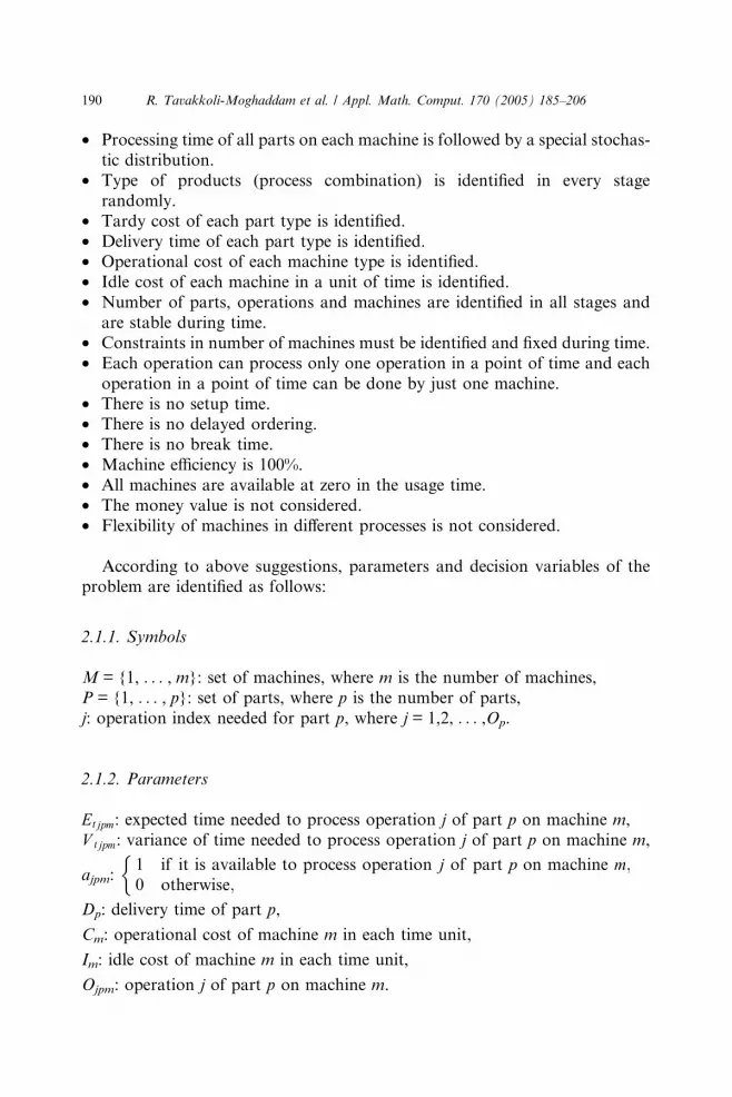
• Each product combination is identified by a special set of parts.


• Processing time of all parts on each machine is followed by a special stochas-

tic distribution.

• Type of products (process combination) is identified in every stage

randomly.

• Tardy cost of each part type is identified.

• Delivery time of each part type is identified.• Operational cost of each machine type is identified.

• Idle cost of each machine in a unit of time is identified.

• Number of parts, operations and machines are identified in all stages and

are stable during time.

• Constraints in number of machines must be identified and fixed during time.

• Each operation can process only one operation in a point of time and each

operation in a point of time can be done by just one machine.

• There is no setup time.• There is no delayed ordering.

• There is no break time.

• Machine efficiency is 100%.

• All machines are available at zero in the usage time.

• The money value is not considered.

• Flexibility of machines in different processes is not considered.

According to above suggestions, parameters and decision variables of theproblem are identified as follows:

2.1.1. Symbols

M = {1, . . . , m}: set of machines, where m is the number of machines,

P = {1, . . . , p}: set of parts, where p is the number of parts,j: operation index needed for part p, where j = 1,2, . . . ,Op.

2.1.2. Parameters

Etjpm: expected time needed to process operation j of part p on machine m,

V tjpm: variance of time needed to process operation j of part p on machine m,

ajpm:1 if it is available to process operation j of part p on machine m;0 otherwise;

�Dp: delivery time of part p,

Cm: operational cost of machine m in each time unit,

Im: idle cost of machine m in each time unit,

Ojpm: operation j of part p on machine m.


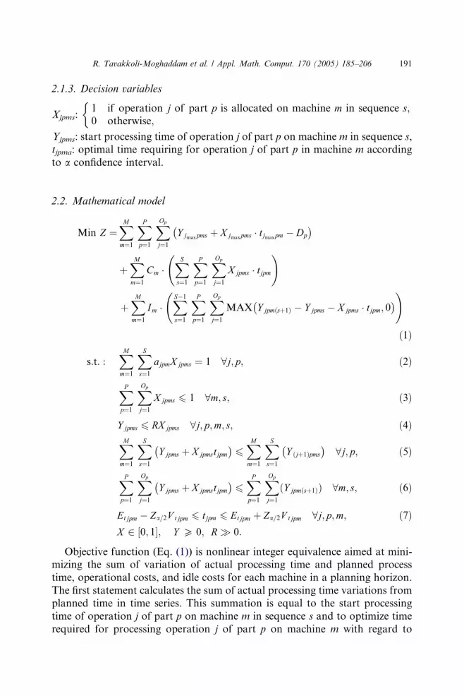
2.1.3. Decision variables

Xjpms:1 if operation j of part p is allocated on machine m in sequence s;0 otherwise;

�Yjpms: start processing time of operation j of part p on machine m in sequence s,

tjpma: optimal time requiring for operation j of part p in machine m according

to a confidence interval.

2.2. Mathematical model

Min Z ¼XMm¼1

XPp¼1

XOp

j¼1Y jmaxpms þ X jmaxpms � tjmaxpm � Dp

� �

þXMm¼1

Cm �XSs¼1

XPp¼1

XOp

j¼1X jpms � tjpm

!

þXMm¼1

Im �XS�1s¼1

XPp¼1

XOp

j¼1MAX Y jpmðsþ1Þ � Y jpms � X jpms � tjpm; 0

� � !

ð1Þ

s:t: :XMm¼1

XSs¼1

ajpmX jpms ¼ 1 8j; p; ð2Þ

XPp¼1

XOp

j¼1X jpms 6 1 8m; s; ð3Þ

Y jpms 6 RX jpms 8j; p;m; s; ð4ÞXMm¼1

XSs¼1

Y jpms þ X jpmstjpm� �

6

XMm¼1

XSs¼1

Y ðjþ1Þpms� �

8j; p; ð5Þ

XPp¼1

XOp

j¼1Y jpms þ X jpmstjpm� �

6

XPp¼1

XOp

j¼1ðY jpmðsþ1ÞÞ 8m; s; ð6Þ

Etjpm � Za=2V tjpm 6 tjpm 6 Etjpm þ Za=2V tjpm 8j; p;m; ð7ÞX 2 ½0; 1�; Y P 0; R � 0:

Objective function (Eq. (1)) is nonlinear integer equivalence aimed at mini-mizing the sum of variation of actual processing time and planned process

time, operational costs, and idle costs for each machine in a planning horizon.

The first statement calculates the sum of actual processing time variations from

planned time in time series. This summation is equal to the start processing

time of operation j of part p on machine m in sequence s and to optimize time

required for processing operation j of part p on machine m with regard to


percent of a confidence interval if this operation has been allocated to the right

machine. The second statement calculates the operational costs of each ma-

chine. This cost is equal to the sum of mutilation of required times for all kinds

of machines in operational cost of that machine. The third statement of the

objective function calculates the idle time of machines. In this case if there is

no part to be allocated to a machine and the machine is idle, there will be idlecost for the machine.

The first constraint (Eq. (2)) guarantees that each operation for each part

must be allocated to just one machine in a sequence. The third equation shows

that only one operation can be in each sequence on a machine. The fourth

equation guarantees that the start processing time is finite. The fifth equation

guarantees the operation sequences for each part. The sixth equation shows

that each operation�s processing time does not have any overlap with anyother. The seventh equation considers a confidence interval for processing ofoperations.

3. Proposed algorithm for the model

Scheduling job shop production systems is complex in calculation and it is

only possible to solve small-scale problems with existing solution algorithms

optimally. The proposed model, dealing with machines flexibility in processingdifferent kind of products, is highly difficult and time consuming to solve opti-

mally for large-scale and real-world problems. This problem highly arises from

resources constraints (time, memory, computers and so forth). In this section,

we propose and present a hybrid algorithm to solve job shop scheduling prob-

lems that enable overcoming many of these resource constraints. Thus, in this

section we present a heuristic algorithm for the solution of the mathematical

model with respect to machines flexibility in processing different kind of prod-

ucts. As mentioned before, there is flexibility for machines to process variousparts. We propose a hybrid method, namely neural networks and a heuristic

algorithm based on simulated annealing, to solve job shop scheduling prob-

lems. In this method, a simulated annealing algorithm can be used individually

or accompany with neural network [8]. The neural network model is used for

eliminating resource and sequence variations resulting in nonfeasible solutions

in a specific problem. The feasible solutions are then optimized through a heu-

ristic algorithm based on simulated annealing. Fig. 1 shows the optimal struc-

ture of the hybrid approach by the use of the simulated annealing algorithm.The solution procedure includes three stages as follows:

(1) To allocate machines to jobs at random with respect to machine flexibility

in processing different products.

(2) To generate the initial or feasible solution by the neural network model.

Neural network

Heuristic algorithm

Feasible solutions

Feasible improved solutionsInitial solutions

Fig. 1. Combinational approach structure.


(3) To improve the quality and performance of the initial solution generated

by neural network model and by simulated annealing algorithm.

Detail descriptions of different stages of heuristic algorithms are presented

below.

Step 1: Allocation jobs to machines at random

Some special processes can be processed on different machines and the abil-ity of processing various parts makes for the possibility of random scheduling

at zero time. The generated solutions caused by random allocation of machines

to parts are the input solutions to the neural network model. This solution is

used to generate the feasible schedule in the next stage.

Step 2: Generating the initial or feasible solution by the neural network model

The proposed nonlinear mathematical model is converted to a neural net-

work design to solve the job shop scheduling problem [8]. To formulate the

suggested job shop model to a neural network, there is a need for three calcu-lation units (neuron) sets according to the following items:

(1) Units related to parts processing time overlap constraint with respect to the

presented sequence of that unit (SC units).

(2) Units related to machines processing time overlap constraint (RC units).

(3) Units related to start processing time for each operation (ST units). The

output of these unites will be a feasible solution of the model. The ST unit

receives inputs from two related SC and RC units and sends output to bothof the units. The ST units have the feedback too.

Activation of SC and RC networks sets is implemented by data entry based

on Yang and Wang [8]. The procedure to generate the production sequence for

various processes is as follows:

(1) Generating the initial or feasible situation: LB numbers of unequal parts

are allocated to each machine randomly. Then, the related operation ineach part is allocated to each machine based on the process requirement.

Machines are allocated to each job at random because of machines flex-

ibility in processing the different operations. In this case, there will be an


initial feasible solution Sikp(0) for each Oikp operation that (i 2 N,

k 2 {1, . . . ,ni}) and this solution can be the net input, ISTikp , for each

ST unit.

(2) Each SC unit, SCikl, of neural SC set activates and calculates the activation

ASCiklðtÞ based on related equivalences. If ASCiklðtÞ 6¼ 0, the sequence con-

straints are not satisfied. In this case, activations will be adjusted by acti-vating related feedbacks, until the constraints are satisfied.

(3) Each SC unit, RCqikjl, of neural RC set activates and calculates the activa-

tion ARCqikjllðtÞ based on related equivalences. If ARCqikjllðtÞ 6¼ 0, the

resources constraints are not satisfied. In this case, activations will be

adjusted by activating Sikq(t + 1), Sjlq(t + 1) feedbacks, until the constraints

are satisfied.

(4) Steps 2 and 3 are reiterated until all the units become stable without any

change. When sequence and resource constraints are satisfied then the fea-sible solution is generated.

(5) The initial solution is used as an input for the heuristic algorithm. Solution

procedure in the heuristic algorithm is developed in the discussion that fol-

lows below.

At the end of this step of the proposed method, the initial feasible solution

will be obtained with regard to the sequence and resource constraints. The next

step after defining the initial solution is to extract an optimal or near-optimalsolution. This is carried out through the use of the heuristic algorithm, as elab-

orated in step 3.

Step 3: Improving the quality and performance of initial solution generated

with neural network model, by simulated annealing (SA) algorithm

In this step, we apply SA to improve the initial sequence obtained from the

previous step [16]. The improvement procedure is implemented by changing

the pair of operations among the machines. In other words, the neighbor

solutions are found by changing the parts among machines. At first, one oper-ation of a job is selected randomly, then one operation from another part is

selected randomly and these two operations change with each other on the

machine. Using SA requires identifying the value of parameters in SA

algorithm.

The initial temperature considers the maximum difference of cost between

neighbor solutions and minimum difference of cost between neighbor solutions.

The neighbor solution is obtained from the initial sequence. The cooling rate

considered as 0.05. The number of iterations in each temperature differs fromanother temperature. Its initial value is equal to five and increases with arith-

metic gradient of five. The algorithm stops when the final temperature reaches

to 0.05. Clearly, the SA program is flexible enough to change all these param-

eters and has ability to implement sensitivity analysis on each of these

parameters.


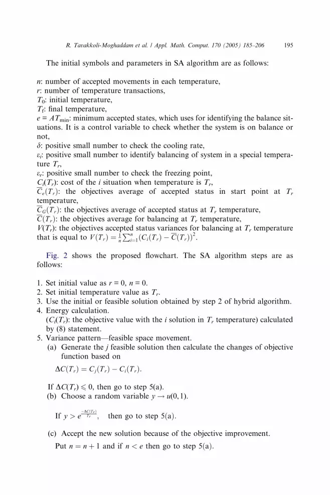
The initial symbols and parameters in SA algorithm are as follows:

n: number of accepted movements in each temperature,

r: number of temperature transactions,

T0: initial temperature,

Tf: final temperature,e = ATmin: minimum accepted states, which uses for identifying the balance sit-

uations. It is a control variable to check whether the system is on balance or

not,

d: positive small number to check the cooling rate,ei: positive small number to identify balancing of system in a special tempera-

ture Tr,

er: positive small number to check the freezing point,Ci(Tr): cost of the i situation when temperature is Tr,CeðT rÞ: the objectives average of accepted status in start point at Tr

temperature,

CGðT rÞ: the objectives average of accepted status at Tr temperature,

CðT rÞ: the objectives average for balancing at Tr temperature,

V(Tr): the objectives accepted status variances for balancing at Tr temperature

that is equal to V ðT rÞ ¼ 1n

Pni¼1ðCiðT rÞ � CðT rÞÞ2.

Fig. 2 shows the proposed flowchart. The SA algorithm steps are asfollows:

1. Set initial value as r = 0, n = 0.

2. Set initial temperature value as Tr.

3. Use the initial or feasible solution obtained by step 2 of hybrid algorithm.

4. Energy calculation.

(Ci(Tr): the objective value with the i solution in Tr temperature) calculated

by (8) statement.5. Variance pattern—feasible space movement.

(a) Generate the j feasible solution then calculate the changes of objective

function based on

DCðT rÞ ¼ CjðT rÞ � CiðT rÞ:

If DC(Tr) 6 0, then go to step 5(a).

(b) Choose a random variable y! u(0,1).

If y > e�DCðT r Þ

T r ; then go to step 5ðaÞ:

(c) Accept the new solution because of the objective improvement.

Put n ¼ nþ 1 and if n < e then go to step 5ðaÞ:

Finish

2. Generate the initial feasible solution by neural network model.

Is the initial solution feasible?

3. Improve the generated sequence

Initial solution with neural network

.Random allocation of jobs to machines

.

Start

1. Random allocation of jobs to machines.

Are all the jobs being scheduled?

No Yes

Yes

No

Fig. 2. Flow chart of the hybrid algorithm.


6. Test for balancing:

Put n = 0, if jCeðT rÞ � CCeðT Þrj > 1 or if the system was not static then go to

step 5(a).

7. Test for freezing point:(a) Calculate V(Tr), CðT rÞ. If r = 0 then go to step 7(a).

IfV ðT Þ

T ðCðT 0Þ � CðT ÞÞ6 e2:

(b) Stop; because of satisfaction.

(c) Update the temperature based on T rþ1 ¼ T r

1þlnð1þoÞT r3V ðT r Þ

. Put r = r + 1 and

then go to step 7(a).


4. Computational results

To evaluate the proposed algorithm, the computer programming in Visual

Basic language was prepared and all the calculations were conducted on a Pen-

tium IV 1800 MHz. For this reason, five sample problems, based on the liter-

ature review, are generated. Due to the complexity of job shop scheduling

problems requiring a large amount of time to generate the optimal solutions,

we consider the lower bound of the solution instead of the optimal solution.

In this paper, we use the Lingo 6 software to get the lower bound of the prob-lem. In this case, the lower bound is less than or equal to the optimal solution.

4.1. Manufacturing systems factors

To generate a series of selected problems, scheduling factors are chosen

among a set of affected variables in sequence. These variables are:

(1) Types of parts: the set of parts needs to be produced. Each part has a spe-cial operation sequence.

(2) Types of machines: the set of machines requires producing types of prod-

ucts. Each machine is able to process more than one operation in different

point of times (i.e., machine flexibility).

(3) Operation sequence of a part: the order of machines that the part needs to

pass on them. The required order and number of operations to produce a

part is identified in this sequence.

(4) Process time: the required time, which need for processing one part on aspecific machine, which is a random variable.

(5) Machine capacity: availability time of each machine to process the parts.

(6) Operational cost: the machine usage cost to process the parts in a unit of

time.

(7) Idle cost: the cost of idle machine in a unit of time.

(8) Tardy cost: the cost of delays in completing the processing of each oper-

ation for each unit of delay time.

(9) Delivery time: specific delivery time for each part.

In the proposed algorithm, all above characteristics are considered. The

problem is investigated under five selected test problems. Table 1 shows the

characteristics of selected problems with factors generated at random.

4.2. Value identification of problem parameters

The next step after generating the selected problems is to identify the values

of required parameters in the problem. The summary of generating value pro-

cedures for selected problems is presented in Table 2.

Table 1

Characteristics of the selected problems to evaluate the proposed algorithms

Run No. of parts No. of machines No. of operations

1 3 2 3

2 5 3 3

3 6 6 6

4 10 10 5

5 20 5 5

Table 2

Parameter characteristics of the selected problems

Scheduling problem factor Amount Description

Maximum of flexibility for each operation 2

Range of process time for each operation [1–10] Uniform distribution

Range of idle cost for each machine [1–5] Uniform discrete distribution

Range of operational cost for each machine [10–15] Uniform discrete distribution

Range of delivery time for each part [10–50] Uniform distribution

Range of tardy cost for each part [1–10] Uniform discrete distribution


4.3. Lower bound generation

We utilize the lower bound solution of the proposed model to compare the

computational results obtained by the proposed hybrid method. It is extremely

difficult to achieve optimal solution within reasonable computational time-

frames due to high complexity of job shop scheduling problems. In this paper,

the Lingo 6 software was used to obtain the lower bound solutions. The close-

ness of the optimal solution generated with hybrid method to lower bound isnot an evaluation of the performance of the hybrid method. Therefore, com-

paring the lower bound with the optimal solution is not verified for making

a decision on the quality performance of the hybrid method.

In this section, we present a test problem solved with the hybrid method.

The Gantt chart and comparison of computational results with the lower

bound are presented. There are some selected problems and their solutions ob-

tained by the hybrid method as well as a comparison of results with the solu-

tion generated by the Lingo 6 software.

4.4. An example problem (3 · 2)

We consider a job shop scheduling problem with three types of parts, 2 ma-

chines, and 3 operations for each job. The completion data of the example is

presented in Tables 3–6. The computational results generated by the hybrid

method and the lower bounds reported by Lingo 6 software are compared in

Table 7.

Table 3

Input data for operation sequence

Operation 1 Operation 2 Operation 3

Part 1 1 2 3

Part 2 0 0 1

Part 3 2 3 1

Table 4

Input data for parts delivery

Part 1 Part 2 Part 3

Tardy cost 7 7 5

Delivery time 34 44 20

Table 5

Input data for machines costs

Machine 1 Machine 2

Idle cost 5 3

Operational cost 13 11


As shown in Table 7, the gap in the objective value between the two methods

is 27.53%. As we considered, the solution obtained by Lingo as a lower bound

of our solution, this value shows the suitable performance of the hybrid meth-

od in generating the near-optimal solution. One of the most important criteria

in generating an optimal or near-optimal solution is the runtime. The hybrid

method has 89.5% time saving than Lingo 6. The amount of saving is highly

significant, especially in large-scale problems.

An important factor in real-world production situations is the makespan ofjobs, Cmax, which is considered in this section with respect to the solutions gen-

erated by Lingo 6 and the hybrid method. We present the Gantt chart of make-

span in each solution procedure in Figs. 3 and 4.

0 10 20 30 40 50 60 70 80 90 100 110 120 130 140 150 160 170 180 190 200 210 220 230

M2

M1

Gant Chart

O23 O11 O31

O33 O21 O13

22 62 137115

73 115 130 226

Fig. 3. Gantt chart of JSSP 3 · 2 using the hybrid method.

le 6

ut data for operation time (Et,Vt)

Part 1 Part 2 Part 3

Operation 1 Operation 2 Operation 3 Operation 1 Operation 2 Op ion 3 Operation 1 Operation 2 Operation 3

chine 1 (41.3,3) (0,0) (23.7,7) (0,0) (0,0) (0,0 (0,0) (24.3,9) (0,0)

chine 2 (29.2,2) (41.7,7) (98.2,2) (15.8,8) (0,0) (0,0 (99.4,4) (54.8,8) (50.2,2)

le 7

parison of results by the hybrid method and Lingo 6

tion procedure No. of iterations Objective value Runtime (s)

rid algorithm 42 3811 729.63

o 6 24 2988.32 6953

ent of difference to Lingo 6 27.53% 89.5%

200

R.Tavakkoli-M

oghaddametal./Appl.Math.Comput.170(2005)185–206

Tab

Inp

Ma

Ma

Tab

Com

Solu

Hyb

Ling

Perc

erat

)

)

0 10 20 30 40 50 60 70 80 90 100 110 120 130 140 150 160 170 180 190 200 210 220 230 240 250 260 270 280 290

M2

M1

Gant Chart

O31 O11

O23

O21 O31 O33

9 60 135129

52 146 192 283

O11

25

Fig. 4. Gantt chart of JSSP 3 · 2 using Lingo.


As shown in Fig. 3, the makespan is equal to 226 time unit, according to the

hybrid method. This value, according to the solution from Lingo 6, is equal to

283 (see Fig. 4). However the objective value by the hybrid method is 27.53%

more than the lower bound while decreasing in runtime and makespan. These

are the main factors to compare and evaluate the efficiency of the proposed

method significantly.

4.5. Calculations of the selected problems

This section presents the solutions of selected problems and the compression

of the associated solutions with the lower bound as well as the analysis of the

related comparison. The aim of these experiments is to identify the perfor-

mance of the hybrid method in different situations. Observations of solutions

and the performance trend of the hybrid method in various problem settings

help us to find the best attributes for using this method in production sched-

ules. The solutions of selected problems are shown in Table 8. The solutionsshow that the hybrid method exhibits good performance in different situations

at most of time and the runtime has been decreased significantly in compare

with the runtime of Lingo 6.

To check problem size effects on the final solution quality, some of the prob-

lems were recalculated based on the sequencing of the Lingo software, and it

was observed that the solutions are improved. The solution comparisons are

presented in Fig. 5. The use of Lingo 6 to generate the lower bound for the

objective function is observed. The difference or gap between the objectivefunction value by the hybrid method and Lingo 6 increases as the problem size

increases. According to the results, it is clear that the hybrid method generates

near-optimal solution in less computational time. It is also clear that the hybrid

method decreases the calculations involved in solving the selected problems to

generate near-optimal solutions. As shown in Fig. 6, the difference or gap be-

tween runtimes and two methods increases as the problem size increases. This

fact shows that the runtime is improved by using the hybrid method to generate

the near-optimal solution.

Table 8

Computational results of selected problems for the hybrid and the lower bound methods

Experiment Types

of parts

Types of

machines

Types of

operations

Solution

algorithm

No. of

iterations

Objective

values

Runtime

(s)

1 3 2 3 Hybrid 42 3811 729.63

Lingo 6 24 2988.32 6953

2 5 3 3 Hybrid 35 8780 1266.8

Lingo 6 5277 3740.28 117,874

3 6 6 6 Hybrid 20,040 20,040 4456.99

Lingo 6 6581.96 6581.96 162,179

4 10 10 5 Hybrid 362 29,547 8547.35

Lingo 6 576 10,352.6 190,800

5 20 5 5 Hybrid 473 37,140 13,548.94

Lingo 6 680 18,254.21 219,600

0

5000

10000

15000

20000

25000

3*2*3 5*3*3 6*6*6 10*5*5 20*5*5Problem size

Obj

ectiv

e va

lue

diffe

renc

e

0

5000

10000

15000

20000

25000

30000

35000

40000

3*2*3 5*3*3 6*6*6 10*5*5 20*5*5

Problem size

Obj

ectiv

e va

lues

(a) Difference in objective values (b) Objective values

* Objective value difference

Hybrid alg.lingo6

Fig. 5. Comparison of objective value for the hybrid and the lower bound methods. (a) Difference

in objective values; (b) objective values.

0

50000

100000

150000

200000

250000

3*2*3 5*3*3 6*6*6 10*5*5 20*5*5

Prob. size

Run

time

diffe

renc

e

020000400006000080000

100000120000140000160000180000200000220000240000

3*2*3 5*3*3 6*6*6 10*5*5 20*5*5

Prob. size

Run

time Runtime1

Runtime2

(a) Runtime difference (b) Runtime

Fig. 6. Comparison of runtime for the hybrid and the lower bound methods. (a) Runtime

difference; (b) runtime.


Lingo6

0

10002000

30004000

5000

60007000

80009000

10000

1100012000

1300014000

15000

1600017000

1800019000

20000

0 10000 20000 30000 40000 50000 60000 70000 80000 90000 100000 110000 120000 130000 140000 150 160000 17000 180000 190000 200000 210000 220000 230000 240000

Time

Obj

ectiv

e va

lue

Fig. 7. Increasing trend on time based on the objective v es using Lingo 6.

R.Tavakkoli-M

oghaddametal./Appl.Math.Comput.170(2005)185–206

203

000

alu

Hybrid

05000

10000

15000200002500030000

3500040000

0 1000 2000 3000 4000 5000 6000 7000 8000 9000 10000 11000 12000 13000 14000 15000

Time

Obj

ectiv

e va

lue

Fig. 8. Increasing trend on time based on objective values from the hybrid algorithm.


As can be observed from Fig. 5, the difference in objective values based on

the hybrid method and Lingo 6 increases as problem size increases, and this is

because of various constraints to solve the large parameters problems by the

optimization software. According to Fig. 6, the difference of runtimes between

two procedures increases exponentially, when the problem size increases. Thecase for using the hybrid method is obvious in problem likely to consume

amount of time in resolution.

Fig. 7 shows that the runtime increases exponentially as the objective value

increases in the Lingo 6 software. However, in hybrid method the slope of the

runtime curve for finding the optimal or near-optimal solution decreases when

the objective values increase, as depicted in Fig. 8.

5. Conclusion

The main reason for this study was to present a procedure for stochastic job

shop scheduling minimizing the difference between the delivery and the comple-

tion times of jobs as well as related operational or idle cost of machines. For

this case, a mathematical programming model was presented after reviewing

the literature survey. To solve the model within reasonable time, a hybrid

method consisting of neural network and simulated annealing (SA) was pro-posed and presented. This method generates the initial feasible solution by neu-

ral network and then simulated annealing algorithm improves the performance

quality of the initial solution. To evaluate the proposed method, we generated

five problems at random and solved them with the proposed method and Lingo

6.

Computational results showed that the hybrid method exhibits high

performance in generating optimal or near-optimal solutions, especially for

large-scale problems. As the problem parameters increase, there is an increasein runtime of Lingo 6 exponentially to generate the lower bound for the given


problem. This time consuming task makes these types of software packages

inapplicable for the solution of large-scale problems. The computational results

show the suitable performance of the hybrid method in extracting acceptable

scheduling solutions within acceptable timeframes. As a result, the proposed

method generates acceptable and better solutions than Lingo 6 for all large-

scale scheduling problems. Thus, the proposed method is recommended forall stochastic scheduling problems with large numbers of machines, parts,

and operations.

As increasing the problem size increases runtime exponentially, it is obvious

that solving large-scale problems is a hugely time consuming task. The pro-

posed method generates the optimal or near-optimal solutions easier and in less

time for large-scale problems containing a large number of constraints. Real-

world manufacturing situations typically feature lots of constraints and param-

eters, so the proposed method is highly relevant for many different industries.The summary of results is as follows:

(1) There is an exponential increase in runtime of Lingo 6, as the problem size

increases. This runtime is almost constant when using the hybrid method in

large-scale problems.

(2) According to the results, the percentage difference in the objective value is

equal to 27.53% in small-sized problems with low number of parts and

machines. This criterion increases for larger-sized problems, containinglarge number of machines and parts. Therefore, it seems that the problem

size has a high effect on solution quality. Moreover, the computational

time increases exponentially, as the problem size increases.

(3) The makespan obtained form the hybrid method (226 time units) is much

better than makespan reported by Lingo 6 (283 time units). This fact is a

highly significant in order to evaluate the performance of scheduling pro-

cedures in real-world production situations. The results show a good per-

formance of the hybrid method in lowering makespan in comparison withLingo 6.

(4) The difference or gap percent increases between these two methods indicat-

ing the relatively superior performance of the hybrid procedure, especially

in resolving larger complex problems.

References

[1] K.R. Baker, Introduction to Sequence and Scheduling, John Wiley, NY, 1974.

[2] R.W. Conway, W.L. Maxwell, Theory of Scheduling, Addison-Wesley, MA, 1967.

[3] D. Dubois, H. Fargier, H. Prade, Fuzzy constraint in job shop scheduling, J. Intell. Manuf. 6

(1995) 215–234.

[4] P.V. Hentenryck, Constant Satisfaction and Logic Programming, MIT Press, MA, 1989.

[5] M.S. Fox, M. Zweben, Knowledge Based Scheduling, Morgan Kaufman, 1993.


[6] A. Johns, L. Rabelo, Survey on job shop scheduling techniques, 1998.

[7] D.G. Ginzburg, A. Gonik, Optimal job-shop scheduling with random operations and cost

objectives, Int. J. Prod. Econ. 76 (2002) 147–157.

[8] S. Yang, D. Wang, Constraint satisfaction adaptive neural network and heuristics combined

approaches for generalized job-shop scheduling, IEEE Trans. Neural Networks 11 (2000) 243–

256.

[9] http://wwwUbka.uni-karlsruhe.de/cgi-bin/psview/, 1997.

[10] H.P.G. Van Ooijen, J.W.M. Bertrand, Economic due-date setting in job-shops based on

routing and workload dependent flow time distribution functions, Int. J. Prod. Econ. 74 (2001)

261–268.

[11] S.E. Elmaghraby, On the optimal release time of jobs with random processing times, with

extensions to other criteria, Int. J. Prod. Econ. 74 (2001) 103–113.

[12] C. Thomalla, Job-shop scheduling with alternative process plans, Int. J. Prod. Econ. 74 (2001)

125–134.

[13] E. Veral, Computer simulation of due-date setting in multi-machine job shops, Comput. Ind.

Eng. 41 (2001) 77–94.

[14] S. Jain, S. Meeran, Job-shop scheduling using neural networks, Int. J. Prod. Res. 36 (1998)

1249–1272.

[15] K.A. Smith, Neural network for combinatorial optimization: A review of more than a decade

of research, Informs J. Comput. 11 (1999) 15–34.

[16] K. Steinhofel, A. Albrecht, C.K. Wong, Two simulated annealing-based heuristics for the job

shops scheduling problem, Eur. J. Operational Res. 118 (1999) 524–548.

http://wwwUbka.uni-karlsruhe.de/cgi-bin/psview/

a hybrid method for solving stochastic job shop scheduling problems

Documents