ARTICLE IN PRESS

European Journal of Operational Research xxx (2005) xxx–xxx

www.elsevier.com/locate/ejor

Discrete Optimization

Network flow approaches to pre-emptive open-shopscheduling problems with time-windows

A. Sedeno-Noda, D. Alcaide *, C. Gonzalez-Martın

Departamento de Estadıstica, Investigacion Operativa y Computacion, University of La Laguna, La Laguna, Tenerife 38204, Spain

Received 13 February 2004; accepted 28 January 2005

Abstract

This paper deals with pre-emptive open-shop scheduling problems with time-windows. Network flow procedures tocheck feasibility and a max-flow parametrical algorithm to minimize the makespan are introduced. Also, computationalcomplexities are evaluated for these feasibility and optimization algorithms. The proposed method is a strongly poly-nomial algorithm to minimize the makespan of the pre-emptive open-shop scheduling problems with time-windowsstrictly respected. Finally, the applications of the proposed algorithms are illustrated with numerical examples.� 2005 Elsevier B.V. All rights reserved.

Keywords: Scheduling problem; Network flow approach; Pre-emptive open-shop; Time-windows; Max-flow parametrical algorithm

1. Introduction

The present paper deals with specialized shop scheduling problems. In these problems the jobs are di-vided into operations and each operation must be performed on the corresponding specialized machine.We propose network flow approaches to check feasibility and to optimize the schedule length criterion.More precisely, the paper focuses on feasibility pre-emptive open-shop problems in which a time-windowis considered for each job. That is, for each job there is a specified time-window defined by its release timeand due date. Feasibility implies that release times are always satisfied and lateness is not permitted (i.e. duedates are, in fact, deadlines). Also, in the paper, the minimization of the makespan is considered. The fea-sibility problem can be denoted by Ojpmtn, rj,djj– and the optimization problem by Ojpmtn, rj,djjCmax

0377-2217/$ - see front matter � 2005 Elsevier B.V. All rights reserved.doi:10.1016/j.ejor.2005.01.062

* Corresponding author. Tel.: +34 922318182; fax: +34 922318170.E-mail address: dalcaide@ull.es (D. Alcaide).

2 A. Sedeno-Noda et al. / European Journal of Operational Research xxx (2005) xxx–xxx

ARTICLE IN PRESS

following the three parameter classification of scheduling problems given by Graham et al. [10] and Lawleret al. [12].

The problem of scheduling a set of jobs on a set of machines, so that all processing conditions are sat-isfied and a certain objective function is optimized, has received extensive attention due to its widespreadapplications. It is well known that scheduling problems are usually very difficult with a great computationalcomplexity. Hence, all the algorithms, models and tools that can be helpful in solving these problems arewelcome. Sometimes network flow models and algorithms may be useful to solve scheduling problems. Thisidea is used by Federgruen and Groenevelt [5]. They study the problem of scheduling n jobs, each with spe-cific processing requirements, release time and due date, on m uniform parallel machines. They show that afeasible schedule can be obtained by determining the maximum flow in a network, thus permitting the useof standard network flow codes. Moreover, their network flow approach reduces the complexity of previousalgorithms that did not use network flow approaches. Federgruen and Groenevelt also prove that this ap-proach is useful not only for the problem of finding feasible solutions, but also for solving some relatedscheduling optimization problems.

Furthermore, Chen [2,3] develops a variant of the classical problem of pre-emptively scheduling indepen-dent jobs with release times and due dates on parallel identical processors. Chen suggests that, in practice,one can often pay to reduce the processing requirement of a job. Then, also using ideas of Federgruen andGroenevelt [5], this variant leads to two parametric max-flow problems. Another different variant is lookedinto by Serafini [15]. He deals with the real problem of scheduling looms in a textile industry. To solve thisproblem, Serafini considers scheduling independent jobs with due dates on multiple machines in the cases ofidentical, uniform or unrelated machines. Thus, in the problems studied by him, the jobs are not dividedinto operations but, the particular type of process he considered allows both for job pre-emption (i.e.any job can be interrupted at any time to process another one) and job splitting (i.e. any job can be splitand processed independently on different machines). Consequently, he considered divisible jobs and piecesof a single job can be simultaneously executed in parallel. In this case, minimizing the maximum weightedtardiness can be done in polynomial time. The case of the contemplated application (uniform machines) canbe modeled as a network flow, and minimization of maximum tardiness can be done in strongly polynomialtime. Serafini also examines the case of unrelated machines, which can be solved either by generalized flowtechniques or by linear programming.

Later, McCormick [13] solved some of the above problems extending the parametric push–relabel max-flow methods originally proposed by Gallo et al. [6].

In the scheduling problems considered in this paper, the attention is mainly focused on pre-emptiveopen-shop scheduling problems with time-windows. In these problems, each job Jj, j = 1, . . . ,n, of the n

jobs to schedule, has its own release time rj and deadline dj. The jobs are divided into operations, to be per-formed on the m specialized machines, and the number of non-zero tasks, i.e., the number of operationswith processing times strictly greater than zero is denoted by l. The paper considers the optimization prob-

lem wherein the objective function selected is to minimize the makespan, that is, the problemOjpmtn, rj,djjCmax.

Note that, as far as we know, there are not many results related to pre-emptive open-shop wherein time-windows are strictly satisfied, i.e. release times and deadlines are respected. In this sense, we can refer toCho and Sahni [4] and Pinedo [14]. Cho and Sahni�s paper deals with pre-emptive open, flow and job shops.With regard to open-shops, Cho and Sahni [4] present a linear programming formulation to find feasibleschedules for the decision problem Ojpmtn, rj,djj–. This formulation is similar to that obtained by Lawlerand Labetoulle [11] for pre-emptive scheduling of unrelated processors. This linear programming can besolved using several times the polynomial time pre-emptive scheduling algorithm of Gonzalez [8] to obtaina pre-emptive schedule (see Gonzalez and Sahni [9]). Moreover, the complexity of this approach is boundedby O(n(l + min{n4,m4, l2})). In addition, Cho and Sahni study special cases of these open-shop feasibilityproblems for which fast algorithms can be obtained. Note that polynomial time algorithms of Cho and Sah-

A. Sedeno-Noda et al. / European Journal of Operational Research xxx (2005) xxx–xxx 3

ARTICLE IN PRESS

ni are restricted to feasibility open-shop problems with a common deadline and additional conditions to thenumbers of machines and different release time values.

Pinedo shows that the feasibility problem subject to release times and deadlines can be solved by linearprogramming. Starting with a solution of the linear program, obtained with any LP solver, the method pre-sented by Pinedo minimizes the maximum lateness (and the makespan) using the procedure that works withthe processing times matrix, and detects sequentially decrementing sets in this matrix (see Section 8.4, pages198–201 in Pinedo [14]).

However, the present paper proposes a different approach, based on network flow algorithms, which al-lows us to solve polynomially more general problems than those which are considered by Cho and Sahni[4], with a different and more efficient approach to that summarized by Pinedo [14]. The present paper pro-poses a strongly polynomial algorithm for solving the feasibility problem Ojpmtn, rj,djj–. The computa-tional complexity is bounded by

O n3 þminfn;mgnl logminfn;mg2

l

!.

In fact, note that, in the worst case l = X(nm), and then our feasibility algorithm runs in O(min {n,m}n2m),improving in one order the complexity of the previous algorithm proposed by Cho and Sahni [4]. In addi-tion, we also propose an

O n3 þminfn;mgnl logminfn;mg2

lþ ðnþ mÞnm log

ðmþ nÞ2

nm

!

algorithm for the optimization problem Ojpmtn, rj,djjCmax.The paper is structured as follows: Section 2 is devoted to describing the problems, emphasising that the

paper mainly focuses on pre-emptive open-shop scheduling problems with time-windows. Mathematicalmodels to solve the feasibility problem, and the optimization open-shop scheduling problem with minimummakespan criterion are presented in this section. Network flow approaches to solve the case under consid-eration are developed in Section 3. This section is divided into two parts. The first one is devoted to thefeasibility open-shop problem. It describes the network proposed to represent this problem, provides amax-flow algorithm to solve it, studies algorithm complexity, and illustrates the algorithm with numericalexamples. The second part deals with the optimization open-shop scheduling problem. A max-flow para-metrical algorithm is proposed to solve the minimum makespan open-shop scheduling problem, the algo-rithm complexity is computed, and a numerical example is reported to illustrate the algorithm. Finally, wesummarize the work providing conclusions in Section 4.

2. Problems description and mathematical models

The following paragraphs are devoted to describing mathematical models for solving Ojpmtn, rj,djjCmax.These results can be easily adapted to solve other feasibility and optimization problems in the open-shopenvironment.

There are m machines M1,M2, . . . ,Mm to perform n jobs J1,J2, . . . ,Jn. Each job Jj is divided into mj

operations. In open shops, without loss of generality, we can suppose that mj = m for all j. We can numberjobs and machines in such a way that operation Oij, i = 1, . . . ,m, j = 1, . . . ,n is the operation of job Jj whichis performed on machineMi. We denote by l the number of operations with processing times strictly greaterthan zero. If there is no confusion, we refer to machine i instead of machine Mi, and job j instead of job Jj.As we are in open-shop problems, the order in which the operations of each job are performed is irrelevant.The only constraints we have are non-overlapping constraints, i.e., it is not possible to perform two or more

4 A. Sedeno-Noda et al. / European Journal of Operational Research xxx (2005) xxx–xxx

ARTICLE IN PRESS

operations of the same job simultaneously, and no machine is able to process two or more different jobssimultaneously.

For each job j = 1, . . . ,n we have the release time rj and the deadline dj. They form a set of K differentvalues with K 6 2n. Let us order these values in non-decreasing order. We have the ordered set {tk,k = 0, . . . ,K � 1} with tk�1 < tk, k = 1, . . . ,K � 1. These milestones determine K � 1 intervals Ik,k = 1, . . . ,K � 1, where Ik = [tk�1, tk] has the positive length Dk = tk � tk�1.

We also have the processing time pij of operation Oij with i = 1, . . . ,m, j = 1, . . . ,n. For notational con-venience, we define the following values:

pi ¼Xnj¼1

pij; 8i ¼ 1; . . . ;m and pj ¼Xmi¼1

pij; 8j ¼ 1; . . . ; n.

Finally, we need to define, the decision variables xijk as the quantity of processing time of the operation Oij

(of job j) assigned to machine i at interval Ik.With this notation, the problem of finding feasible schedules for the decision problem Ojpmtn, rj,djj–, can

be formulated with the following linear programming problem according to the classical linear program-ming formulation pointed out by Cho and Sahni [4] and similar that the formulation summarized in Pinedo[14].

This linear program has the following constraints:

xijk P 0; 8i 2 f1; . . . ;mg; 8j 2 f1; . . . ; ng; 8k 2 f1; . . . ;K � 1g; ð1Þ

Xmi¼1

xijk 6 Dk; 8j 2 f1; . . . ; ng; 8k 2 f1; . . . ;K � 1g; ð2Þ

Xnj¼1

xijk 6 Dk; 8i 2 f1; . . . ;mg; 8k 2 f1; . . . ;K � 1g; ð3Þ

XK�1

k¼1

xijk ¼ pij; 8i 2 f1; . . . ;mg; 8j 2 f1; . . . ; ng; ð4Þ

tk�1 < rj or dj < tk ) xijk ¼ 0; 8i 2 f1; . . . ;mg; 8j 2 f1; . . . ; ng; 8k 2 f1; . . . ;K � 1g ð5Þ

(i.e., if Ik = [tk�1, tk] X [rj,dj] ) xijk = 0, "i 2 {1, . . . ,m}, "j 2 {1, . . . ,n}, "k 2 {1, . . . ,K � 1}).Inequalities (1) mean that the quantity of processing time of operation Oij assigned to interval Ik must be

non-negative. Constraints (2) mean that the total assigned processing amount of job j at interval Ik is smal-ler than or equal to the interval length (avoid overlapping of job j). Inequalities (3) indicate that the quan-tity of processing assigned to machine i (of the different jobs) at interval Ik is not bigger than the intervallength (avoid overbooking of machine i). Eqs. (4) mean that the total processing amount of operation Oij

assigned to the different intervals (Ik, k = 1, . . . ,K � 1) must be equal to its own processing time pij for fea-sibility. Constraints (5) guarantee that time-windows are strictly satisfied, i.e., there is no operation of anyjob j performed either before instant rj or after instant dj. Note that constraints (2)–(4) assure that the quan-tity of processing time of operation Oij assigned to interval Ik does not exceed its own processing time andthe interval length. Then, each feasible schedule verifies constraints (1)–(5). Reciprocally, for each set ofdecision variables values X = {xijk, i = 1, . . . ,m, j = 1, . . . ,n, k = 1, . . . ,K � 1} such that X satisfies (1)–(5) we can identify a solution where there is no job overlapping, there is no machine overbooking, thejob time-windows are respected, and the total processing amount of each operation Oij is exactly its ownprocessing time pij, that is, we can identify a feasible schedule.

A. Sedeno-Noda et al. / European Journal of Operational Research xxx (2005) xxx–xxx 5

ARTICLE IN PRESS

Let us define Fk as the maximum amount of processing time units than can be processed in the intervalsIt, with t = 1, . . . ,k, satisfying constraints (1)–(5) for these intervals.

In the next section, we will introduce an approach to obtain the values Fk for all k. For now, we onlyneed the meaning of these values. Now, let us to define k* as the index of the first interval such thatF k� ¼

Pmi¼1

Pnj¼1pij. If such interval does not exist, then there is not feasible solution for problem (1)–(5).

Otherwise, we can find a feasible schedule satisfying the constraints (1)–(5) with k varying from 1 to k*.Moreover, k* is the smallest index of interval needed to find a feasible solution. In addition, if we define

fk ¼F 1 if k ¼ 1;

F k � F k�1 if k > 1;

�8k ¼ 1; . . . ; k� ð6Þ

that is, fk is the greater augmentation of processing time units from value Fk�1 that can be achieved whenthe interval Ik is used additionally. Now, the next result holds:

Proposition 1. For any feasible schedule using the first k* intervals, fk� is the minimum processing time unitsthat can be processed in the interval Ik� , when in the previous intervals F k��1 time units are processed.

Proof. Since fk� ¼ F k� � F k��1 ¼Pm

i¼1

Pnj¼1pij � F k��1 and F k��1 is the greatest amount of unit times pro-

cessed using the intervals 1, . . . ,k* � 1, it is clear that fk� is minimum. h

From Proposition 1, the following result can be iteratively proved:

Proposition 2. Fixed any index k from 1 to k*, fk is the minimum processing time units that can be processed in

the interval Ik, when in the intervals I1, . . . , Ik�1 Fk�1 time units are processed.

From previous definitions and propositions, it is clear that a feasible schedule using the first k* intervalsand processing fk time units at the kth interval for all k = 1, . . . ,k* can be found. We use this property todesign an efficient algorithm later.

Now, let us consider the optimization problem where the aim is to minimize the makespan (Cmax). Givena feasible schedule S, i.e., S satisfied (1)–(5), Cj(S) is the completion time of job j, i.e., the instant in whichthe processing of job j is concluded in solution S. The makespan of this solution is Cmax(S) =maxj = 1, . . . , n{Cj(S)}. Minimizing makespan is to find a feasible schedule S* such that Cmax(S*) =min{Cmax(S)/S is a feasible schedule}. So, when pre-emptive open-shop scheduling problems with time-windows are considered, and the objective is to minimize the makespan, it is easy to see that the problemcould be formulated in the form

min Cmax

s.t. (1)–(5).

As it is well-known, for each feasible solution S, if k = k(S) is the minimum number of intervals needed tomake schedule S, it is verified that tk�1 6 Cmax(S) 6 tk, i.e., the makespan associated to S is achieved insidethe interval Ik = [tk�1, tk]. Moreover,

CmaxðSÞ ¼ tk�1 þmax maxj¼1;...;n

Xmi¼1

xijk

( ); max

i¼1;...;m

Xnj¼1

xijk

( )( ).

We have the following result for the makespan problem:

Corollary 1. According to Proposition 1, it follows immediately that

(i) The number of intervals used for every optimal solution of the makespan minimization problem (Cmax)isexactly k*.

6 A. Sedeno-Noda et al. / European Journal of Operational Research xxx (2005) xxx–xxx

ARTICLE IN PRESS

(ii) The number of processed time units in the interval Ik� for each optimal solution of the makespan minimi-

zation problem (Cmax) is greater or equal than fk� . In addition, in whose optimal solutions such that there

are F k��1 time units processed in the previous intervals, the aforementioned number is exactly fk� .

Finally, once k* is known, the problem of minimal makespan can be formulated as

min max maxj¼1;...;n

Xmi¼1

xijk�

( ); max

i¼1;...;m

Xnj¼1

xijk�

( )( )

s.t. (1)--(5) ðwith k ¼ 1; . . . ; k�Þ.ð7Þ

3. Network flow approaches

This section describes the network flow models and max-flow algorithms proposed to solve the problemsconsidered in the previous sections. That is, the problem of finding feasible schedules for the decision prob-lem Ojpmtn, rj,djj– and the optimization problem Ojpmtn, rj,djjCmax. Algorithm complexities are studiedand illustrative numerical examples are given. General aspects of network flow approaches can be consultedin Ahuja et al. [1].

3.1. Open-shop feasibility problems

Let us start with open-shop feasibility problems. To do it easily, let us introduce the variables Yjk, andZki, where Y jk ¼

Pmi¼1xijk, the total quantity of job j assigned to the different machines at interval Ik, and

Zki ¼Pn

j¼1xijk, the total quantity of processing time of the different jobs assigned to machine i at intervalIk, "i 2 {1, . . . ,m}, "j 2 {1, . . . ,n}, "k 2 {1, . . . ,K � 1} (where Yjk is defined if, and only if, Ik [rj,dj]).Additionally, we define Xk

ij ¼Pk

t¼1xijt, Zki ¼

Pkt¼1Zti and Y k

j ¼Pk

t¼1Y jt, as the accumulated processing timeunits, in the first k intervals, of the operation Oij, of the machine i, and of the job j, respectively.

With these notations, and taking into account (1) and (3), it is clear that

0 6 Zki ¼Xnj¼1

xijk 6 Dk; 8i 2 f1; . . . ;mg; 8k 2 f1; . . . ;K � 1g. ð8Þ

We also have that

0 6 Y jk ¼Xmi¼1

xijk 6 Dk; 8j 2 f1; . . . ; ng; 8k 2 f1; . . . ;K � 1g; such that Y jk is defined; ð9Þ

where we used (1) and (2).From (1) and (4), it is clear that

0 6 Xkij 6 pij; 8i 2 f1; . . . ;mg; 8j 2 f1; . . . ; ng; 8k 2 f1; . . . ;K � 1g. ð10Þ

In the other hand, and using (8) and (9), we have that

0 6 Zki 6

Xkt¼1

Dt; 8i 2 f1; . . . ;mg; 8k 2 f1; . . . ;K � 1g; ð11Þ

0 6 Y kj 6

Xkt¼1

dtjDt; 8j 2 f1; . . . ; ng; 8k 2 f1; . . . ;K � 1g; ð12Þ

A. Sedeno-Noda et al. / European Journal of Operational Research xxx (2005) xxx–xxx 7

ARTICLE IN PRESS

where

dtj ¼1 if ðtt�1; ttÞ ½rj; dj�;0 otherwise.

�

Then, we have already formulated the problem of obtaining the values of Fk for all values of k. This prob-lem leads to determine the value of k* and the values of fk, "k 2 {1, . . . ,k*}. For this, we introduce the nextmax-flow problem denoted as problem Fk:

max F k

s:t:Xnj¼1

X kij � Zk

i ¼ 0; 8i 2 f1; . . . ;mg;

Y kj �

Xmi¼1

X kij ¼ 0; 8j 2 f1; . . . ; ng;

Xnj¼1

Y kj ¼ F k;

Xmi¼1

Zki ¼ F k;

0 6 Zki 6

Xkt¼1

Dt; 0 6 Y kj 6

Xkt¼1

dtjDt; 0 6 X kij 6 pij.

For k = 1, the solution of the above problem give us the greatest number of processing time units that canbe made into the interval I1 satisfying machine and job restrictions. The above problem is iterativelysolved until finding an index k* such that F k� ¼

Pmi¼1

Pnj¼1pij or determining that there is not a feasible

schedule.The problem Fk is solved using the bipartite directed network given in Fig. 1. This network has one

source node s, one sink node t, m machine nodes and n job nodes. The arcs are directed from source nodeto machine nodes, from machine nodes to job nodes and from job nodes to sink node. The capacity of thesearcs for problem Fk are

Pkt¼1Dt, pij and

Pkt¼1dtjDt, respectively.

Thus, the algorithm to compute the values Fk for all values of k and to determine the value of k* has thefollowing scheme, where we use as subroutine the algorithm of Goldberg and Tarjan [7] due to the networkis bipartite:

M1

M2

Mm

s t

J1

J2

Jn

1

k

tt=

∆∑ijp

1

δ=∑

k

tjt

∆t

Fig. 1. Network for the problem Fk.

8 A. Sedeno-Noda et al. / European Journal of Operational Research xxx (2005) xxx–xxx

ARTICLE IN PRESS

ACCUMULATED PROCESSING TIME UNITS (APTU) ALGORITHM

begink := 0;Repeat

k := k + 1; Fk := 0;Solve problem Fk in the network showed in Fig.1 and store the value of Fk;

Until F k ¼Pm

i¼1

Pnj¼1pij or k = K � 1;

If F k <Pm

i¼1

Pnj¼1pij then

The scheduling problem is unfeasible

elsebegink*: = k; f1: = F1;for k: = 2 to k* do fk: = Fk � FK�1

endend;

Once the APTU algorithm is applied, we know if a feasible schedule exists. In the positive case, we havedetermined the value of k* and the values of fk, "k 2 {1, . . . ,k*}. Now, we must to determine the way todistribute the processing time units fk carried out into the interval Ik for the different machines and jobs, forall values of k. For this, we must to take into account that

Pk�

k¼1Zki ¼ pi andPk�

k¼1Y jk ¼ pj. In this way, wecan formulate the following two feasibility flow problems:

Machine max-flow problem

Job max-flow problem

Xmi¼1

Zki ¼ fk; 8k 2 f1; . . . ; k�g

Xnj¼1

Y jk defined

Y jk ¼ fk; 8k 2 f1; . . . ; k�g

Xk�k¼1

Zki ¼ pi; 8i 2 f1; . . . ;mg

Xk�k¼1

Y jk defined

Y jk ¼ pj; 8j 2 f1; . . . ; ng

0 6 Zki 6 Dk, "i 2 {1, . . . ,m},

0 6 Yjk 6 Dk, "j 2 {1, . . . ,n}, "k 2 {1, . . . ,k*} "k 2 {1, . . . ,k*} such that Yjk is defined

Note that in the above problems, once the values of fk, "k 2 {1, . . . ,k*}, are known, both problems canbe solved separately. In this case, the problem regarding to variables Zki consists of determining a feasiblesolution of a capacitated transportation problem. This problem can be solved using a max-flow algorithm(Machine max-flow problem). In similar way, we obtain the Job max-flow problem. These problems aresolved on networks shown in Fig. 2.

The network for Machine max-flow problem has one source node s, one sink node t, k* interval nodesand m machine nodes. The arcs are directed from source node to interval nodes, from interval nodes tomachine nodes (representing the decision variables Zki) and from machine nodes to sink node. The capacityof these arcs are fk, Dk and pi, respectively (Fig. 2a). The network for Job max-flow problem has one source

M1

M2

Mm

s t

fk ∆kpi

Ik*

I1

Ik*

I1

J1

J2

J

s t

fk∆kpj

(a) (b)

Fig. 2. Network for Machine max-flow problem (a) and Job max-flow problem (b).

A. Sedeno-Noda et al. / European Journal of Operational Research xxx (2005) xxx–xxx 9

ARTICLE IN PRESS

node s, one sink node t, n job nodes and k* interval nodes. The arcs are directed from source node to jobnodes, from job nodes to interval nodes (representing the decision variables Yjk) and from interval nodes tosink node. The capacity of these arcs are pj, Dk and fk, respectively (Fig. 2b). Note, that there is a job-inter-val arc, say arc (Jj, Ik) if, and only if, it is possible to process such job Jj in interval Ik, i.e. Ik [rj,dj].

It is important to remark that both previous networks are bipartite networks. Thus, we use as a subrou-tine the algorithm of Goldberg and Tarjan [7] to solve these max-flow problems. The algorithm can be de-scribed in the following way:

FEASIBILITY OPEN-SHOP ALGORITHM

beginSolve the Machine max-flow problem in the network showed in Fig.2a to obtain the

values of Zki;Solve the Job max-flow problem in the network showed in Fig.2b to obtain the val-

ues of Yjk;end;

After solving Machine and Job max-flow problems, we have values for the variables Yjk, "j 2 {1, . . . ,n},"k 2 {1, . . . ,k*}, such that Yjk is defined, and Zki, "i 2 {1, . . . ,m}, "k 2 {1, . . . ,k*}, that allow us to ob-tain a feasible solution. To finally solve the original open-shop feasibility problem (1)–(5), the algorithmmust compute the unknown values of the variables xijk from the known values of variables Yjk and Zki.That is, for a fixed k, we must to solve the following feasibility problem:

Xm

i¼1

xijk ¼ Y jk; 8j 2 f1; . . . ; ng; ð13Þ

Xnj¼1

xijk ¼ Zki; 8i 2 f1; . . . ;mg; ð14Þ

0 6 xijk 6 uij; 8i 2 f1; . . . ;mg; 8j 2 f1; . . . ; ng; ð15Þ

where uij is a known upper bound of the value xijk at the fixed interval k. Note that, the sum of the valuesYjk and Zki for all k, force to satisfy constraint (4). The above problem consists of determining a feasiblesolution of a capacitated transportation problem. This feasible solution can be determined solving a max-flow problem. Thus, our algorithm solves k* max-flow problems posed by constraints (13)–(15) using theGoldberg–Tarjan algorithm. The capacity uij is initialized to pij for above problem with k = 1. Once the kth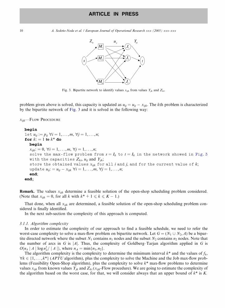

M1

M2

Mm

s t

Zki Yjk

J1

J2

Jn

uij

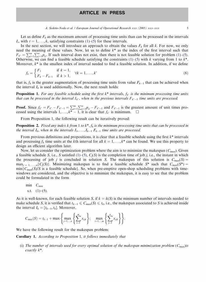
Fig. 3. Bipartite network to identify values xijk from values Yjk and Zki.

10 A. Sedeno-Noda et al. / European Journal of Operational Research xxx (2005) xxx–xxx

ARTICLE IN PRESS

problem given above is solved, this capacity is updated as uij = uij � xijk. The kth problem is characterizedby the bipartite network of Fig. 3 and it is solved in the following way:

xijk—FLOW PROCEDURE

beginlet uij := pij "i = 1, . . . ,m, "j = 1, . . . ,n;for k: = 1 to k* do

beginxijk: = 0, "i = 1, . . . ,m, "j = 1, . . . ,n;solve the max-flow problem from s = Ik to t = Ik in the network showed in Fig.3

with the capacities Zki, uij and Yjk;store the obtained values xijk for all i and j, and for the current value of k;update uij: = uij � xijk "i = 1, . . . ,m, "j = 1, . . . ,n;end;

end;

Remark. The values xijk determine a feasible solution of the open-shop scheduling problem considered.(Note that xijk = 0, for all k with k* + 1 6 k 6 K � 1.)

That done, when all xijk are determined, a feasible solution of the open-shop scheduling problem con-sidered is finally identified.

In the next sub-section the complexity of this approach is computed.

3.1.1. Algorithm complexity

In order to estimate the complexity of our approach to find a feasible schedule, we need to refer theworst-case complexity to solve a max-flow problem on bipartite network. Let G = (N1 [ N2,A) be a bipar-tite directed network where the subset N1 contains n1 nodes and the subset N2 contains n2 nodes. Note thatthe number of arcs in G is jAj. Thus, the complexity of Goldberg–Tarjan algorithm applied in G isOðnA j A j log n2A= j A jÞ, where nA = min{n1,n2}.

The algorithm complexity is the complexity to determine the minimum interval k* and the values of fk,"k 2 {1, . . . ,k*} (APTU algorithm), plus the complexity to solve the Machine and the Job max-flow prob-lems (Feasibility Open-Shop algorithm), plus the complexity to solve k* max-flow problems to determinevalues xijk from known values Yjk and Zki (xijk-Flow procedure). We are going to estimate the complexity ofthe algorithm based on the worst case, for that, we will consider always that an upper bound of k* is K.

A. Sedeno-Noda et al. / European Journal of Operational Research xxx (2005) xxx–xxx 11

ARTICLE IN PRESS

The running time of the APTU algorithm equals k* 6 K times the complexity of Golberg–Tarjan algo-rithm applied to the network depicted in Fig. 1. Note that, in this bipartite network jAj = l + m + n for allproblems Fk. Thus, this complexity is given by:

APTU algorithm Only dominant terms

O Kminfm; ngðlþ mþ nÞ logminfm; ng2

lþ mþ n

!O minfm; ngKl logminfm; ng2

l

!

The complexity of Feasibility Open-Shop algorithm equals to the sum of the effort solving the Machineand Job max-flow problems using Goldberg–Tarjan algorithm, that is:

Only dominant terms

Machine max-flow problem

O minfK;mgðKmþ K þ mÞ log minfK;mg2

Kmþ K þ m

!O(min{K,m}Km)

Job max-flow problem

O minfK; ngðKnþ K þ nÞ log minfK; ng2

Knþ K þ n

!O(min{K,n}Kn)

The complexity of xijk-Flow procedure equals k* 6 K times the complexity of Goldberg–Tarjan algo-rithm applied to the network from Fig. 2 (note that in this case jAj = l + m + n), that is:

xijk-Flow procedure Only dominant terms

O Kminfm; ngðlþ mþ nÞ logminfm; ng2

lþ mþ n

!O minfm; ngKl logminfm; ng2

l

!

Using the fact that K 6 2n and considering only dominant terms, the overall complexity of the algorithmis bounded by

O n3 þminfn;mgnl logminfn;mg2

l

!. ð16Þ

Example. The following numerical data correspond to a pre-emptive open-shop scheduling problem. Weare applying the previous algorithm to find feasible solutions where tardy jobs are not allowed.

There are n = 3 jobs to be processed by m = 3 specialized machines. Operation Oij of job j is processedby machine i and its processing time is pij where i = 1, 2, 3 and j = 1, 2, 3. Job j has release time rj and dead-line dj. These values determine the time-window [rj,dj] for each job j. Table 1 collects these data.

With these data the intervals Ik for k = 1, . . . ,K � 1 are I1 = [0, 5] and I2 = [5, 11] with lengths D1 = 5and D2 = 6 and, thus, K � 1 = 2.

M1

M2

M3

s t

J1

J2

J3

5

5

5

5

5

5

1

42

23

2

1

1

1∆ijp

1∆1δ j M1

M2

M3

s t

J1

J2

J3

11

11 11

1111

5

1

42

23

2

1

1

1 2∆ + ∆ 1 1 2 jδ δ∆ ∆2jijp

(a) (b)

+

Fig. 4. Network for problem F1 (a) and F2 (b).

Table 1Input data for the numerical example

j = 1 j = 2 j = 3

Release time rj 0 0 0Deadline dj 5 11 11Processing times pij

i = 1 1 4 2i = 2 2 3 2i = 3 1 0 1

12 A. Sedeno-Noda et al. / European Journal of Operational Research xxx (2005) xxx–xxx

ARTICLE IN PRESS

The methodology proposed in this paper requires calculating the values of Fk with k = 1, . . . ,k* usingAPTU algorithm. In Fig. 4a the network for problem F1 is shown. In this case, the value of the maximumflow in this network is F1 = 12 and, as F 1 <

Pmi¼1

Pnj¼1pij ¼ 16, we consider the next interval. The network

for problem F2 is depicted in Fig. 4b. When the Golberg–Tarjan algorithm is applied on this network, weobtain F2 = 16. In this case, F 2 ¼

Pmi¼1

Pnj¼1pij and, therefore, k* = 2. Moreover, f2 = F2 � F1 = 4 and

f1 = F1 = 12 are the minimum processing time units need, to carry out in each of these intervals, to obtaina feasible schedule.

Now, from the values of fk with k = 1, . . . ,k*, the Machine and Job max-flow problems are solved. Thenetworks for both problems are depicted in Fig. 5.

Next, applying the Feasibility Open-Shop algorithm, we obtain the values Zki and Yjk for all i = 1, 2, 3,j = 1, 2, 3 and k = 1, 2. These values are tabulated in Table 2.

Next, to identify this solution, it is necessary to detect values xijk from values Zki, Yjk. It is done by solv-ing k* = 2 max-flow problems as xijk-Flow procedure indicates. The initial networks for iterations k = 1and k = 2 are shown in Fig. 6.

M1

M2

Mm

s t

fk ∆kpi

I2

I1

5

55

6

6

6

12

4

7

7

2 I2

I1

J1

J2

J3

s t

fk∆kpj

4

7

5 5

5

5

6

6

12

4

(a) (b)

Fig. 5. Network for Machine max-flow problem (a) and Job max-flow problem (b).

Table 2Zki and Yjk values

i, j k = 1 k = 2

Zki Yjk Zki Yjk

1 5 4 2 –2 5 3 2 43 2 5 0 0

M1

M2

M3

s t

Z1 i Yj1

J1

J2

J3

uij

5

5

2

4

3

5

1

42

23

2

1

1

M1

M2

M3

s t

Z2 i Yj2

J1

J2

J3

uij

2

2

0

0

4

0

2

2

(a) (b)

Fig. 6. Bipartite network for k = 1 (a) and k = 2 (b).

1 3

2 3 1 2

3 1 2 2

0 1 2 4 5 7 9 11

Fig. 7. Gantt diagram for a feasible solution provided by the algorithm.

A. Sedeno-Noda et al. / European Journal of Operational Research xxx (2005) xxx–xxx 13

ARTICLE IN PRESS

Fig. 6a shows the network for the max-flow problem (13)–(15) for k = 1 with uij = pij for all machine-jobarc. Once this problem is solved, the values of variables xijk are x111 = 1, x121 = 2, x131 = 2, x211 = 2,x221 = 1, x231 = 2, x311 = 1, x321 = 0, x331 = 1; and a new max-flow problem (13)–(15) for k = 2 is formu-lated with uij = pij � xij1 for all machine-job arc. The initial network of this problem is showed in Fig. 6b.Note that machine-job arcs with uij = 0 do not appear. In the last case, it is only possible the solutionx122 = 2, x222 = 2.

According to the above values of variables xijk, a feasible solution where tardy jobs are not allowed isdrawn in Fig. 7.

The following subsection is devoted to open-shop optimization problems.

3.2. Open-shop optimization: minimizing makespan (Cmax)

Let us consider the open-shop optimization problem where the objective is to minimize the makespan(Cmax). This problem is described in Section 2. To solve this problem we make use of the previous efforts

14 A. Sedeno-Noda et al. / European Journal of Operational Research xxx (2005) xxx–xxx

ARTICLE IN PRESS

developed to solve the associated feasibility problem. We also make use of the theoretical results given inSection 2.

From (7) and using variables Yjk, "j 2 {1, . . . ,n}, "k 2 {1, . . . ,k*}, such that Yjk is defined, and Zki,"i 2 {1, . . . ,m}, "k 2 {1, . . . ,k*}, it is clear that the minimal makespan can be formulated as

min max maxj¼1;...;n

Y jk� defined

fY jk�g; maxi¼1;...;mfZk�ig

8><>:

9>=>;

s:t: (1)--(5) ðwith k ¼ 1; . . . ; k�Þ.

Also, once the values fk, "k 2 {1, . . . ,k*} are known and, from Corollary 1, the above problem is equiv-alent to

Machine parametric max-flow problem

Job parametric max-flow problem

mink

mink

s:t:Xmi¼1

Zki ¼ fk 8k 2 f1; . . . ; k�g

s:t:Xnj¼1

Y jk defined

Y jk ¼ fk 8k 2 f1; . . . ; k�g

Xk�k¼1

Zki ¼ pi 8i 2 f1; . . . ;mg

Xk�k¼1

Y jk defined

Y jk ¼ pj 8j 2 f1; . . . ; ng

0 6 Zki 6 Dk "k 2 {1, . . . ,k* � 1},

0 6 Yjk 6 Dk "j 2 {1, . . . ,n}, "i 2 {1, . . . ,m} "k 2 {1, . . . ,k* � 1} such thatYjk is defined

0 6 Zk�i 6 minfk;Dk�g 8i 2 f1; . . . ;mg

0 6 Y jk� 6 minfk;Dk�g 8j ¼ 1; . . . ; n such that Y jk� is defined

Note that the above problems are parametric Machine and Job max-flow problems with the same k. Theseproblems are posed by networks shown in Fig. 2 where only the flow on the interval-machine and job-inter-val arcs for node interval Ik� are bounded by k. It is clear, that both parametric max-flow problems can besolved by iteratively solving the Machine and Job max-flow problem with a fixed value of k until

Xmi¼1

Zk�i andXnj¼1

Y jk defined

Y jk�

become equal to fk� .For that, we need an initial value of k. It is clear that the Cmax value is bounded, i.e.

tk��1 þmax fk�m

� �; fk�

n�

� �� �6 Cmax 6 tk��1 þ fk� , where n* is the number of jobs able to be processed at the

k*th interval. Then, an initial value of k is

k0 ¼ maxfk�

m

� �;

fk�

n�

� �� �.

It is chosen to distribute, in an equitable way if it is possible, the fk� processing time units among the ma-chines (the jobs). Such distribution implies that the value of Cmax is, exactly, its lower bound.

A. Sedeno-Noda et al. / European Journal of Operational Research xxx (2005) xxx–xxx 15

ARTICLE IN PRESS

In order to simplify the explanation of the method, we only explain the way to solve the parametric Ma-chine max-flow problem (the parametric Job max-flow problem is solved in an analogous way). First, wesolve the Machine max-flow problem with k = k0. If

Pmi¼1Zk�i < fk� , then we define m(k0) as the number of

machines i such that Zk�i ¼ k0. It is clear that, in this case it is necessary to increase the value of the capacityk0 to find feasibility. Note also that, if Zk�i < k0 for any i, it means that the increasing of the capacity k0 doesnot lead to increasing

Pmi¼1Zk�i. In other words, the arcs that can belong to the minimum cut are the arcs

with Zk�i ¼ k0 with i = 1, . . . ,m and, thus, they are the arcs in which the capacity must be increased in a fairand equitable way. Thus, finished an iteration p, the next iteration start with

kpþ1 ¼ kp þ fk� �Pm

i¼1Zk�i

mðkpÞ

� �.

Once the parametric Machine max-flow problem is solved, for example, the algorithm ends with kp, theparametric Job max-flow problem starts with k = kp. If

Xnj¼1

Y jk defined

Y jk� < fk� ;

then we define n(kp) as the number of jobs j such that Y jk� ¼ kp and update kp by

kpþ1 ¼ kp þ

fk� �Pnj¼1

Y jk� defined

Y jk�

nðkpÞ

266666666

377777777

and solve the job max-flow problem until

Xnj¼1

Y jk� defined

Y jk� ¼ fk� .

It is obvious that the value of the makespan is C�max ¼ tk��1 þ kp, where kp is the last k-value found, and the

makespan Cmax is minimal.Now, we are in a position to present the following method.

ALGORITHM TO MINIMIZE Cmax (MAX-FLOW PARAMETRICAL ALGORITHM)

beginOnce the values fk for k = 1, . . . ,k* are obtained using APTU algorithm

(there is a feasible schedule);

Compute k0 ¼ maxf fk�m e; d

fk�n� e

� �where n* is the number of jobs able

to be processed at interval Ik� ; p: = 0 (the iteration counter);While

Pmi¼1Zk�i < fk� do {parametric Machine max-flow problem}

beginSolve the Machine max-flow problem in the network showed in

Fig.2a, taking into account the value of kp, to obtain the

values of Zki;IfPm

i¼1Zk�i < fk� then

16 A. Sedeno-Noda et al. / European Journal of Operational Research xxx (2005) xxx–xxx

ARTICLE IN PRESS

begin

kpþ1 ¼ kp þ fk��Pm

i¼1Zk� i

mðkpÞ

� �;

p: = p + 1end

end;While

Pnj¼1

Y jk� defined

Yjk� < fk� do {parametric Job max-flow problem}

beginSolve the Job max-flow problem in the network showed in Fig.2b,

taking into account the value of kp, to obtain the values of

Yjk;If

Pnj¼1

Y jk� defined

Yjk� < fk� then

begin

kpþ1 ¼ kp þ

fk� �Pnj¼1

Y jk� defined

Yjk�

nðkpÞ

266666666

377777777

;

p: = p + 1end

endend.

Again, we must compute the unknown values of the variables xijk from the known values of variables Yjk

and Zki that minimizing the makespan. For that, we use xijk-Flow procedure.

3.2.1. Algorithm complexity

Since solving a parametric max-flow problem on bipartite networks given in Fig. 2, using Gallo, Grigor-iadis and Tarjan algorithm, [6], requires a computational effort of

O ðnþ KÞKn log ðnþ KÞ2

Knþ ðmþ KÞKm log

ðmþ KÞ2

Km

!

and, considering only dominant terms and that K = O(n), we obtain

O n3 þ ðnþ mÞnm logðmþ nÞ2

nm

!. ð17Þ

Thus, we can affirm that the overall complexity of minimize the makespan open-shop scheduling problemis equal to the complexity of find a feasible open-shop schedule plus (17), that is, the followingexpression:

O n3 þminfn;mgnl logminfn;mg2

lþ ðnþ mÞnm log

ðmþ nÞ2

nm

!. ð18Þ

I2

I1

J1

J2

J3

s t

fk∆kpj

4

7

5 5

5

5

2

2

12

4

Fig. 8. Network for Job max-flow problem with k = 2.

1 3

2 31

3 1 2

0 1 2 4 5 7 9 11

Fig. 9. Gantt diagram for the optimal solution provided by the algorithm (C�max ¼ 7).

A. Sedeno-Noda et al. / European Journal of Operational Research xxx (2005) xxx–xxx 17

ARTICLE IN PRESS

Example. Let us consider the pre-emptive open-shop scheduling problem, wherein late jobs are forbidden,the input data of which are described in Table 1. We are now interested in minimizing makespan using theoptimization algorithm proposed.

Following the algorithm, we have k* = 2, fk� ¼ 4, n* = 2 and m = 3, then

k0 ¼ max4

3

� �;

4

2

� �� �¼ 2.

Note that the values given in Table 2 for the Machine max-flow problem satisfy Zk�i 6 k0. Therefore, for theparametric Machine max-flow problem, the values Z11 = 5, Z12 = 5, Z13 = 2; Z21 = 2, Z22 = 2, andZ23 = 0 do not change. However, for the parametric Job max-flow problem, the values shown in Table2 do not satisfy Y jk� 6 k0 (for example, Y22 = 4). Thus, we need to solve the Job max-flow problem k0 = 2.

The network for this case is showed in Fig. 8. Note that the capacities of the arcs representing variablesY jk� equals minfDk� ; k

0g ¼ minf6; 2g ¼ 2, for j = 2, 3. Once this Job max-flow problem is solved, we obtainY11 = 4, Y21 = 5, Y31 = 3; Y12 = 0, Y22 = 2, Y32 = 2. Note that these values differ from the values showedin Table 2. Moreover, since Y 22 þ Y 32 ¼ fk� ¼ 4, we can find a feasible open-shop solution minimizing themakespan.

Thus, the optimal value of the makespan is C�max ¼ k0 þ tk��1 ¼ 2þ 5 ¼ 7. Finally, once xijk�-flow proce-

dure is applied, we obtain the optimal solution drawn in Fig. 9.

4. Conclusions

Some previous references inform us that the use of network flow approaches may be useful to solve sat-isfactorily certain scheduling problems with identical or uniform machines, that is only cases with parallel

18 A. Sedeno-Noda et al. / European Journal of Operational Research xxx (2005) xxx–xxx

ARTICLE IN PRESS

and no specialized machines. The presented paper considers both feasibility and optimization schedulingproblems with specialized machines in the case of pre-emptive open-shop with time-windows. The paperdevelops network flow procedures to check feasibility and a max-flow parametrical algorithm to minimizethe makespan in this scheduling case. The computational complexities of these feasibility and optimizationalgorithms are evaluated and numerical examples are reported to illustrate the proposed algorithms better.It is important to note that, as far as we know, the proposed algorithm to minimize the makespan in thepre-emptive open-shop scheduling problems with time-windows strictly respected is the first strongly poly-nomial combinatorial algorithm presented to solve this scheduling case.

Acknowledgments

The authors wish to thank anonymous referees for their constructive and useful suggestions. This workhas been partially supported by Spanish Government Research Projects DPI2001-2715-C02-02 andMTM2004-07550, which are helped by European Funds of Regional Development, and University ofLa Laguna Research Project 180221024.

References

[1] R. Ahuja, T. Magnanti, J.B. Orlin, Network Flows, Prentice-Hall, 1993.[2] Y.L. Chen, Scheduling jobs to minimize total cost, European Journal of Operational Research 74 (1994) 111–119.[3] Y.L. Chen, A parametric maximum flow algorithm for bipartite graphs with applications, European Journal of Operations

Research 80 (1995) 226–235.[4] Y. Cho, S. Sahni, Preemptive scheduling of independent jobs with release and due times on open, flow and job shops, Operations

Research 29 (1981) 511–522.[5] A. Federgruen, H. Groenevelt, Preemptive scheduling of uniform machines by ordinary network flow techniques, Management

Science 32 (3) (1986) 341–349.[6] G. Gallo, M.D. Grigoriadis, R.E. Tarjan, A fast parametric maximum flow algorithm and applications, SIAM Journal of

Computing 18 (1) (1989) 30–55.[7] A.V. Goldberg, R.E. Tarjan, A new approach to the maximum flow problem, in: Proc. 18th ACM Symp. on the Theory of

Computation, 1986, pp. 136–146.[8] T. Gonzalez, A note on open shop preemptive schedules, Technical Report No. 214, Computer Science Dept., Pennsylvania State

University, 1976.[9] T. Gonzalez, S. Sahni, Open shop scheduling to minimize finish time, Journal of the Association Computing Machine 23 (1976)

665–679.[10] R.L. Graham, E.L. Lawler, J.K. Lenstra, A.H.G. Rinnooy Kan, Optimization and approximation in deterministic sequencing

and scheduling: A survey, Annals of Discrete Mathematics 5 (1979) 287–326.[11] E.L. Lawler, J. Labetoulle, On preemptive scheduling of unrelated parallel processors by linear programming, Journal of the

Association Computing Machine 25 (1978) 612–619.[12] E.L. Lawler, J.K. Lenstra, A.H.G. Rinnooy Kan, D. Shmoys, Sequencing and scheduling: Algorithms and complexity, in:

Graves S.C., A.H.G. Rinnooy Kan, P.H. Zipkin (Eds.), Handbooks in Operations Research and Management Science, vol. 4,North Holland, 1993, Chapter 9.

[13] S.T. McCormick, Fast algorithms for parametric scheduling come from extensions to parametric maximum flow, OperationsResearch 47 (5) (1999) 744–756.

[14] M. Pinedo, Scheduling: Theory, Algorithms and Systems, Prentice-Hall, 2002.[15] P. Serafini, Scheduling jobs on several machines with the job splitting property, Operations Research 44 (4) (1996) 617–628.