a declarative debugging system for lazy functional logic programs
TRANSCRIPT
Electronic Notes in Theoretical Computer Science 64 (2002)URL: http://www.elsevier.nl/locate/entcs/volume64.html 63 pages
A Declarative Debugging System forLazy Functional Logic Programs
Rafael Caballero 1,2 Mario Rodrıguez-Artalejo 1,3
Dep. Sistemas Informaticos y ProgramacionUniversidad Complutense Madrid
Madrid, Spain
Abstract
We present a declarative debugger for lazy functional logic programs with poly-morphic type discipline. Whenever a computed answer is considered wrong by theuser (error symptom), the debugger locates a program fragment (function definingrule) responsible for the error. The notions of symptom and error have a declara-tive meaning w.r.t. to an intended program semantics. Debugging is performed bysearching in a computation tree which is a logical representation of the computa-tion. Following a known technique, our tool is based on a program transformation:transformed programs return computation trees along with the results expected bysource programs. Our transformation is provably correct w.r.t. well-typing and pro-gram semantics. As additional improvements w.r.t. related approaches, we solve apreviously open problem concerning the use of curried functions, and we provide acorrect method for avoiding redundant questions to the user during debugging. Aprototype implementation of the debugger is available. Case studies and extensionsare planned as future work.
1 Introduction
The impact of declarative languages on practical applications is inhibited bymany known factors, including the lack of debugging tools, whose constructionis recognized as difficult for lazy functional languages. As argued in [29], suchdebuggers are needed, and much of interest can still be learned from theirconstruction and use. Debugging tools for lazy functional logic languages [11]are even harder to construct.
1 Work partially supported by the Spanish CICYT (project CICYT-TIC98-0445-C03-02/97“TREND”)2 Email: [email protected] Email: [email protected]
c©2002 Published by Elsevier Science B. V.
Caballero and Rodrıguez-Artalejo
A promising approach is declarative debugging, which starts from a compu-tation considered incorrect by the user (error symptom) and locates a pro-gram fragment responsible for the error. In the case of (constraint) logicprograms, error symptoms can be either wrong or missing computed answers[26,13,6,17,28]. Declarative debugging has been also adapted to lazy functionalprogramming [21,22,23,27,18,20,25] and combined functional logic program-ming [19]. All these approaches use a computation tree (CT) [19] as logicalrepresentation of the computation. Each node in a CT represents the result ofa computation step, which must follow from the results of its children nodesby some logical inference. Diagnosis proceeds by traversing the CT, askingquestions to an external oracle (generally the user) until a so-called buggy nodeis found, whose result is erroneous, but whose children have all correct results.The user does not need to understand the computation operationally. Anybuggy node represents an erroneous computation step, an the debugger candisplay the program fragment responsible for it. From an explanatory pointof view, declarative debugging can be described as consisting of two stages,namely CT generation and CT navigation [22].
We present a declarative debugger of wrong answers for lazy functional logicprograms with polymorphic type discipline. Following a known idea [22,20,25],we use a program transformation for CT generation. We give a careful speci-fication of the transformation, we show its advantages w.r.t. previous relatedones, and we describe some new techniques which allow to avoid redundantquestions to the oracle during the navigation phase.The debugger has beenimplemented as part of the T OY system [14]; a prototype version can bedownloaded from http://titan.sip.ucm.es/toy/. Case studies and exten-sions of the debugger are planned as future work.
A known extension of declarative debugging is abstract diagnosis [3,1], leadingto equivalent bottom-up and top-down diagnosis methods which do not requireerror symptoms to be given in advance. In order to be effectively implemented,abstract diagnosis uses abstract interpretation techniques to build a finiteabstraction of the intended program semantics. These methods are outsidethe scope of this paper.
The rest of the paper is organized as follows: Section 2 recalls preliminarynotions and previous results about functional logic programming and declar-ative debugging. Section 3 summarizes our new contributions w.r.t. previousrelated works. Our approaches to CT generation and navigation, with detailedexplanations of the new contributions, are presented in Sections 4 and 5, re-spectively. Conclusions and plans for future work are summarized in Section6. Detailed proofs of the main results are included in the Appendix A, whileAppendix B includes some simple debugging sessions.
2
Caballero and Rodrıguez-Artalejo
2 Preliminaries
Functional Logic Programming (FLP for short) aims at the integration of thebest features of current functional and logic languages; see [11] for a survey.This paper deals with declarative debugging for lazy FLP languages suchas Curry or T OY [12,14], which include pure LP and lazy FP programs asparticular cases. In this section we recall the basic facts about syntax, typediscipline and declarative semantics for lazy FLP programs. We follow theformalization given in [9], but using the concrete syntax of T OY for programexamples.
2.1 Types, Expressions and Substitutions
2.1.1 Types and Signatures
We assume a countable set TV ar of type variables α, β, . . . and a countableranked alphabet TC =
⋃
n∈N TCn of type constructors C. Types τ ∈ Type
have the syntax
τ ::= α (α ∈ TV ar) | (C τ1 . . . τn) (C ∈ TCn) | (τ → τ ′) | (τ1, . . . , τn)
By convention, C τn abbreviates (C τ1 . . . τn), “→” associates to the right,τn → τ abbreviates τ1 → · · · → τn → τ , and the set of type variables occurringin τ is written tvar(τ). A type τ is called monomorphic iff tvar(τ) = ∅, andpolymorphic otherwise. A type without any occurrence of “→” is called adatatype.
A polymorphic signature over TC is a triple Σ = 〈TC, DC, FS〉, whereDC =
⋃
n∈NDCn and FS =
⋃
n∈N FSn are ranked sets of data constructors
resp. defined function symbols. Each n-ary c ∈ DCn comes with a principaltype declaration c :: τn → C αk, where n, k ≥ 0, α1, . . . , αk are pairwisedifferent, τi are datatypes, and tvar(τi) ⊆ {α1,. . . , αk} for all 1 ≤ i ≤ n(so-called transparency property). Also, every n-ary f ∈ FSn comes with aprincipal type declaration f :: τn → τ , where τi, τ are arbitrary types. Inpractice, each FLP program P has a signature which corresponds to the typedeclarations occurring in P . For any signature Σ, we write Σ⊥ for the resultof extending Σ with a new data constructor ⊥ :: α, intended to representan undefined value that belongs to every type. As notational conventions,we use c, d ∈ DC, f, g ∈ FS and h ∈ DC ∪ FS, and we define the arity ofh ∈ DCn ∪ FSn as ar(h) = n.
2.1.2 Expressions and Patterns
In the sequel, we always suppose a given signature Σ, often not made explicitin the notation. Assuming a countable set V ar of (data) variables X, Y, . . .disjoint from TV ar and Σ, partial expressions e ∈ Exp⊥ have the syntax
e ::= ⊥ | X | h | (e e′) | (e1, . . . , en)
3
Caballero and Rodrıguez-Artalejo
where X ∈ V ar, h ∈ DC ∪ FS. Expressions of the form (e e′) stand for theapplication of expression e (acting as a function) to expression e′ (acting asan argument), while expressions (e1, . . . , en) represent tuples with n compo-nents. As usual, we assume that application associates to the left and thus(e0 e1 . . . en) abbreviates ((. . . (e0 e1) . . .) en). The set of data variables occur-ring in e is written var(e). An expression e is called closed iff var(e) = ∅,and open otherwise. Moreover, e is called linear iff every X ∈ var(e) has onesingle occurrence in e. Partial patterns t ∈ Pat⊥ ⊂ Exp⊥are built as
t ::=⊥ | X | c t1 . . . tm | f t1 . . . tm | (t1, . . . , tn)
where X ∈ V ar, c ∈ DCn, 0 ≤ m ≤ n, f ∈ FSn, 0 ≤ m < n and ti partialpatterns for all 1 ≤ i ≤ m. They represent approximations of the valuesof expressions. Following the spirit of denotational semantics [10], we viewPat⊥ as the set of finite elements of a semantic domain, and we define theapproximation ordering v as the least partial ordering over Pat⊥ satisfyingthe following properties:
• ⊥ v t, for all t ∈ Pat⊥.
• h tm v h sm whenever these two expressions are patterns and ti v si for all1 ≤ i ≤ m.
• (t1, . . . , tn) v (s1, . . . , sn) whenever ti, si ∈ Pat⊥, ti v si for all 1 ≤ i ≤ m.
Pat⊥, and more generally any partially ordered set (shortly, poset), can beconverted into a semantic domain by means of a technique called ideal com-pletion; see e.g. [16].
Partial patterns of the form f t1 . . . tm with f ∈ FSn and m < n serve asa convenient representation of functions as values; see [9]. Expressions andpatterns without any occurrence of ⊥ are called total. We write Exp andPat for the sets of total expressions and patterns, respectively. Actually, thesymbol ⊥ never occurs in a program’s text; but it may occur in a debuggingsession, as we will see.
2.1.3 Substitutions
A total substitution is a mapping θ : V ar → Pat with a unique extension θ :Exp→ Exp, which will be noted also as θ. The set of all substitutions is notedas Subst. The set of all the partial substitutions θ : V ar → Pat⊥ is denoted asSubst⊥ and defined analogously. We define the domain dom(θ) as the set of allvariables X s.t. θ(X) 6= X, and the range ran(θ) as
⋃
X∈dom(θ) var(θ(X)). As
usual, θ = {X1 7→ t1, . . . , Xn 7→ tn} stands for the substitution with domain{X1, . . . , Xn} which satisfies θ(Xi) = ti for all 1 ≤ i ≤ n. By convention,we write eθ instead of θ(e), and θσ for the composition of θ and σ, such thate(θσ) = (eθ)σ for any e. For any subset X ⊆ dom(θ) we define the restrictionθ �X as the substitution θ′ such that dom(θ′) = X and θ′(X) = θ(X) for allX ∈ A. We also define the disjoint union θ1∪· θ2 of two given substitutions with
4
Caballero and Rodrıguez-Artalejo
disjoint domains, as the substitution θ such that dom(θ) = dom(θ1)∪dom(θ2),θ(X) = θ1(X) for all X ∈ dom(θ1), and θ(Y ) = θ2(Y ) for all Y ∈ dom(θ2).
The identity mapping id from V ar onto itself is called the identity substitution,and any substitution ρ which behaves as a bijective mapping from V ar ontoitself is called a renaming. Two expressions e and e′ are called variants iffthere is some renaming ρ such that eρ = e′. The subsumption ordering overExp is defined by the condition e ≤ e′ iff e′ = eθ for some θ ∈ Subst. Asimilar ordering can be defined over Exp⊥, and extended to work over Subst⊥by defining θ ≤ θ′ iff θ′ = θσ for some σ ∈ Subst⊥. For any set of datavariables X , we use the notations θ ≤ θ′[X ] (resp. θ ≤ θ′[\X ]) to indicatethat Xθ′ = Xθσ holds for some σ ∈ Subst⊥ and all X ∈ X (resp. all X 6∈ X ).Another useful notion is the approximation ordering over Subst⊥, defined bythe condition θ v θ′ iff θ(X) v θ′(X), for all X ∈ V ar.Up to this point we have considered data substitutions. Type substitutionscan be defined similarly, as mappings θt : TV ar → Type with a uniqueextension θt : Type→ Type, noted also as θt. The set of all type substitutionsis noted as TSubst. Most of the concepts and notations presented above fordata substitutions (such as domain, range, composition, renaming, etc.) makesense also for type substitutions, and we will freely use them when needed.
2.1.4 Well-typed Expressions
Inspired by Milner’s type system [15,4] we now introduce the notion of well-typed expression. We define a type environment as any set T of type assump-tions X :: τ for data variables, such that T does not include two different as-sumptions for the same variable. The domain dom(T ) and the range ran(T )of a type environment are the set of all data variables resp. type variablesthat occur in T . For any variable X ∈ dom(T ), the unique type τ such that(X :: τ) ∈ T is noted as T (X). The notation (h :: τ) ∈var Σ is used toindicate that Σ includes the type declaration h :: τ up to a renaming of typevariables.
Type judgements (Σ, T ) `WT e :: τ are derived by means of the following typeinference rules:
VR (Σ, T ) `WT X :: τ , if T (X) = τ
ID (Σ, T ) `WT h :: τσt,
if (h :: τ) ∈var Σ⊥, σt ∈ TSubst
AP (Σ, T ) `WT (e e1) :: τ ,
if (Σ, T ) `WT e :: (τ1 → τ), (Σ, T ) `WT e1 :: τ1, for some τ1 ∈ Type
TP (Σ, T ) `WT (e1, . . . , en) :: (τ1, . . . , τn),
if (Σ, T ) `WT e1 :: τ1, . . . , (Σ, T ) `WT en :: τnNote that the previous type inference rules can deal with polimorphic types,
5
Caballero and Rodrıguez-Artalejo
because the type declarations included in the signature Σ are interpreted astype schemes, as seen in the inference rule ID.
We will abbreviate a sequence (Σ, T ) `WT e1 :: τ1, . . . , (Σ, T ) `WT en :: τnas (Σ, T ) `WT en :: τn , while (Σ, T ) `WT a :: τ, (Σ, T ) `WT b :: τ will beabbreviated as (Σ, T ) `WT a :: τ :: b.
An expression e ∈ Exp⊥ is called well-typed iff there exist some type environ-ment T and some type τ , such that the type judgement T `WT e :: τ can bederived. Expressions that admit more than one type are called polymorphic.A well-typed expression always admits a so-called principal type (PT) that ismore general than any other. A pattern whose PT determines the PTs of itssubpatterns is called transparent. See [9] for more details.
2.2 Programs and Goals
2.2.1 Well-typed Programs
A well-typed program P is a set of well-typed defining rules for the functionsymbols in its signature. Defining rules for f ∈ FSn with principal type dec-laration f :: τn → τ have the form
(R) f t1 . . . tn︸ ︷︷ ︸
left-hand side
→ r︸︷︷︸
right-hand side
⇐ C︸︷︷︸
condition
and must satisfy the following requirements:
(i) t1 . . . tn is a linear sequence of transparent patterns and r is an expression.
(ii) The condition C is a sequence of atomic conditions C1, . . . , Ck, whereeach Ci can be either a joinability statement of the form e == e′, withe, e′ ∈ Exp, or an approximation statement of the form d → s, withd ∈ Exp and s ∈ Pat.
(iii) Moreover, the condition C must be admissible w.r.t. the set of variablesX =def var(f tn). By definition, this means that the set of all theapproximation statements occurring in C must admit some sequentialarrangement, say d1 → s1, · · · , dm → sm (m ≥ 0), such that the threeproperties below hold:(a) For all 1 ≤ i ≤ m: var(si) ∩ X = ∅(b) For all 1 ≤ i ≤ m, si is linear and for all 1 ≤ j ≤ m with i 6= j
var(si) ∩ var(sj) = ∅.(c) For all 1 ≤ i ≤ m, 1 ≤ j ≤ i: var(si) ∩ var(dj) = ∅.
(iv) There is some type environment T with domain var(R), which well-typesthe definining rule in the following sense:(a) For all 1 ≤ i ≤ n: (Σ, T ) `WT ti :: τi.(b) (Σ, T ) `WT r :: τ .(c) For each (e == e′) ∈ C there is some µ ∈ Type
such that (Σ, T ) `WT e :: µ :: e′.
6
Caballero and Rodrıguez-Artalejo
(d) For each (d→ s) ∈ C there is some µ ∈ Typesuch that (Σ, T ) `WT d :: µ :: s.
In the programming language T OY [14] program rules are written in a some-what different way, namely:
(R) f t1 . . . tn︸ ︷︷ ︸
left-hand side
→ r︸︷︷︸
right-hand side
⇐ JC︸︷︷︸
joinability conditions
where LD︸︷︷︸
local definitions
In this syntax, the condition C of a program rule is split in two parts: onepart JC consisting of joinability statements e == e′, and another part LDconsisting of approximation statements d → s, which are understood as lo-cal definitions for the variables occurring in the pattern s. This motivatesrequirement (iii) above. In fact:
• Items (iii) (a), (iii) (b) require the locally defined variables to be differentfrom each other and away from the variables occurring in the rule’s left-handside, that act as formal parameters.
• Item (iii) (c) ensures that variables defined in local definition number i canbe used in local definition number j only if j > i. In particular, this meansthat the local definitions cannot be recursive.
Informally, the intended meaning of a program rule like (R) above is that acall to function f can be reduced to r whenever the actual parameters matchthe patterns ti, and both the joinability conditions and local definitions aresatisfied. A condition e == e′ is satisfied by evaluating e and e′ to somecommon total pattern. A local definition d → s is satisfied by evaluating dto some possibly partial pattern which matches s. A precise formulation ofprogram semantics will be presented in Section 2.3.
2.2.2 A Simple Program
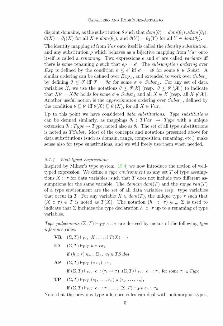
Below we show a simple example program, written in the concrete syntax ofthe T OY language. In this syntax, local definitions d → s are written ass ← d, and they must appear in a textual order which shows fulfilment ofthe admissibility requirements explained in Section 2.2.1. T OY also allowsto use infix operators such as : to build expressions such as (X:Xs), whichis understood as ((:) X Xs). The signature of the program can be easilyinferred from the type declarations included in its text. In particular, the datadeclarations give complete information about the type constructors and theprincipal types of the data constructors.
% data [A] = [] | A : [A]
head :: [A] → A tail :: [A] → [A]head (X:Xs) → X tail (X:Xs) → Xs
7

Caballero and Rodrıguez-Artalejo
map :: (A → B) → [A] → [B] twice :: (A → A) → A → Amap F [] → [] twice F X → F (F X)map F (X:Xs) → F X : map F Xs
drop4 :: [A] → [A] from :: nat → [nat]drop4 → twice twice tail from N → N : from N
data nat = z | suc nat
plus :: nat → nat → nat times :: nat → nat → natplus z Y → Y times z Y → zplus (suc X) Y → suc (plus X Y) times (suc X) Y → plus (times X Y) X
take :: nat → [A] → [A] (//) :: A → A → Atake z Xs → [] X // Y → Xtake (suc N) [] → [] X // Y → Ytake (suc N) (X:Xs) → X : take N Xs
data person = john | mary | peter | paul | sally | molly | rose | tom |bob | lisa | alan | dolly | jim | alice
parents :: person → (person,person)parents peter → (john,mary) parents alan → (paul,rose)parents paul → (john,mary) parents dolly → (paul,rose)parents sally → (john,mary) parents jim → (tom,sally)parents bob → (peter,molly) parents alice → (tom,sally)parents lisa → (peter,molly)
ancestor :: person → personancestor X → Y // Z // ancestor Y // ancestor Z
where (Y,Z) ← parents X
% data bool = true | false
related :: person → person → boolrelated X Y → true <= ancestor X == ancestor Y
The data declarations for the types of lists and boolean values are includedmerely as comments, since these types are predefined in T OY. Note that thelist constructors are noted as [] and : (an infix operator), as in Haskell [24].The intended meaning of the functions should be clear from their names anddefinitions. The arity of each function is always the same as the number of for-mal parameters in its rules. In particular, drop4 (a function which eliminatesthe first four elements of a given list) has arity 0, in spite of its type. The lasttwo functions illustrate the use of joinability conditions and local definitions.Moreover, the functions ancestor and (//) are non-deterministic, since a callto them with fixed parameters can return more than one result. For instance,ancestor alan can return any of the results paul, rose, john or mary.
8
Caballero and Rodrıguez-Artalejo
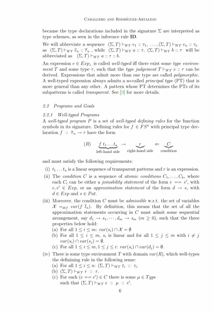
Some of the program rules in this example are incorrect w.r.t. the intendedmeaning of the corresponding functions. More precisely, the second rule fortimes and the single rule for from are wrong; their correct versions should be:
times (suc X) Y → plus (times X Y) Y from N → N : from (suc N)
In the next section we will give a formal definition of “intended meaning”,which is needed to prove mathematical results about the correctness of declar-ative debugging.
2.2.3 Well-typed Goals
A well-typed goal G has the same form as a well-typed condition. In particular,it must satisfy the admissibility requirements explained in Section 2.2.1, butnow w.r.t. the empty set of variables. A FLP system is expected to solve goals,returning substitutions θ as computed answers. For the simple program fromSection 2.2.1, some examples of goals and answers which can be computed bythe T OY system are:
(i) The goal related alan X == true has the computed answer {X 7→ alice}(among others).
(ii) The goal take (suc (suc z)) (from X) == Xs has a single computed answer,namely {Xs 7→ X:X:[]}, which is wrong w.r.t. the intended meaning of theprogram.
(iii) The goal head (tail (map (times N) (from X))) == Y asks for the secondelement of the infinite list that contains the product of N by the consecu-tive natural numbers starting at X. The first two solutions computed byT OY are {N 7→ z, Y 7→ z} (which is correct) and {N 7→ suc z, Y 7→ z}(which is wrong). This is because the buggy function times causes theexpression (times (suc z)) to return always the result z. The valid solution{N 7→ suc z, Y 7→ suc X} expected by the user is in fact a missing answer.Diagnosing missing answers is beyond the scope of this paper.
2.3 Program Semantics
2.3.1 The Semantic Calculus SC
In [9], a rewriting calculus called GORC was used to deduce from a givenprogram P those approximation and joinability statements which should beconsidered as valid according to P ’s semantics. Informally, an approximationstatement e → t means that t ∈ Pat⊥ represents a partially defined valuewhich approximates the value of e ∈ Exp⊥; while a joinability statemente == e′ means that e→ t, e′ → t holds for some total t ∈ Pat.In this paper we will use the Semantic Calculus SC, a variant of GORC whichwas first proposed in [2] in order to define a logically correct framework forthe declarative debugging of wrongs answers in lazy FLP languages. Formally,SC consists of the following inference rules:
9
Caballero and Rodrıguez-Artalejo
BT e→⊥
RR X → X with X ∈ V ar
DC e1 → t1 . . . em → tm h tm ∈ Pat⊥h em → h tm
JN e→ t e′ → t t ∈ Pat (total pattern)e == e′
C r → s
AR+FA e1 → t1 . . . en → tnf tn → s s ak → t (f tn → r ⇐ C) ∈ [P ]⊥,
f en ak → t t 6=⊥
In all the SC rules, e, ei ∈ Exp⊥ are partial expressions, ti, t, s ∈ Pat⊥ arepartial patterns and h ∈ DC ∪ FS. The notation [P ]⊥ in rule AR + FAstands for the set {(l → r ⇐ C)θ | (l → r ⇐ C) ∈ P, θ ∈ Subst⊥} ofpartial instances of the rules from P . The labels of the different inferencerules have the following intended meanings: BT stands for Bottom, RR forrestricted reflexivity, DC for decomposition, JN for joinability and AR + FAfor argument reduction + function application.
Notice that AR+FA is the only SC rule which depends on the given program.It must be understood as the consecutive application of two inference steps,whose separate specification is displayed below:
AR e1 → t1 . . . en → tn f tn → s s ak → t f ∈ FSn
f en ak → t t 6=⊥
FA C r → s (f tn → r ⇐ C) ∈ [P ]⊥f tn → s
The rule AR+FA formalizes the steps to be performed for computing a partialpattern t as approximated value for the function application f en ak, namely:
(i) Compute suitable partial patterns ti as approximated values for the ar-gument expressions ei.
(ii) Apply a program rule instance (f tn → r ⇐ C) ∈ [P ]⊥, verify thecondition C, and compute a suitable partial pattern s as approximatedvalue for the right-hand side r.
(iii) Compute t as approximated value for s ak.
Working with partial patterns here allows to specify non-strict semantics withthe syntactic simplicity of strict semantics. In the case k > 0, f must bea higher-order function which returns a functional value, represented by thepattern s. In the case k = 0, the rule AR + FA can be simplified by takingf tn → t as the conclusion of the FA step, and omitting the premise s ak → t.We will implicitly assume this simplification all along the paper.
10
Caballero and Rodrıguez-Artalejo
Note that SC cannot apply the two inference rules AR and FA independently;they must be always used within a combined AR + FA step. Nevertheless,to think of the FA steps within a given SC proof is helpful, because onlysuch steps depend on program rules. Moreover, the conclusions of FA stepsare particularly simple approximation statements of the form f tn → s (withti, s ∈ Pat⊥), which will be called basic facts in the rest of the paper. Bothbasic facts and local definitions are approximation statements, but they areused for different purposes. A basic fact f tn → s asserts that the (possiblynon-linear) partial pattern s approximates the result of f tn, a call function callwith the exact number of arguments expected by f ’s arity, and with argumentsti ∈ Pat⊥, which represent the partial approximations of f ’s actual parametersneeded to compute s as result.
The other inference rules in SC are easier to understand. In the sequel we usethe notation P `SC ϕ is used to indicate that the statement ϕ can be deducedfrom the program P using the SC inference rules. For instance, taking asP the simple program from Section 2.2.2, the following SC derivations arepossible:
(i) P `SC from X → X:⊥.
(ii) P `SC from X → X:X:⊥.
(iii) P `SC parents alice → (tom,sally).
(iv) P `SC ancestor alan → john.
(v) P `SC ancestor alan → mary.
(vi) P `SC ancestor alice → john.
(vii) P `SC ancestor alice → mary.
(viii) P `SC ancestor alan == ancestor alice.
These examples show that the semantics of approximation statements is con-sistent with their use as local definitions within programs, but different fromthe meaning of equality. For instance, from X → X:⊥ only means that thepartial value X:⊥ approximates the value of (from X), not that the value of(from X) is equal to X:⊥. There is a formal relationship between approxima-tion statements and the approximation ordering over Pat⊥ defined in Section2.1.2. This and other basic properties of SC are stated in the following re-sult, which can be proved by straightforward induction on the structure of SCproofs 4 .
Proposition 2.1 For any given program P :(i) For all t, s ∈ Pat⊥: P `SC t→ s iff t w s.
4 The proof of a similar result for first-order programs can be found in [8].
11
Caballero and Rodrıguez-Artalejo
take (suc (suc z)) (from X) → X:X:[ ]((((((((((((((
�������
hhhhhhhhhhhAR+FA
suc (suc z) → suc (suc z)
DC∗from X → X:X:⊥
SS�������
AR+FA
take (suc (suc z)) (X:X:⊥) → X:X:[ ]
X → X
RR
from X → X:X:⊥ X: take (suc z) (X:⊥) → X:X:[ ]
SS
DC
X:from X → X:X:⊥
SS�������DC
X → X
RR
take (suc z) (X:⊥) → X:[ ]
SS
��������
((((((((((((AR+FA
X → X
RR
from X → X:⊥
SS
�������AR+FA
suc z → suc z
DC∗X:⊥ → X:⊥DC,RR,BT
take (suc z) (X:⊥) → X:[ ]
X → X
RR
from X → X:⊥ X:take z ⊥ → X:[ ]
SS
�������DC
X:from X → X:⊥
SS
������� DC
X → X
RR
take z ⊥ → [ ]
SS
�����
��������AR+FA
X → X
RR
from X → ⊥BT
z → z
DC
⊥ → ⊥BT
take z ⊥ → [ ]
[ ] → [ ]
DC
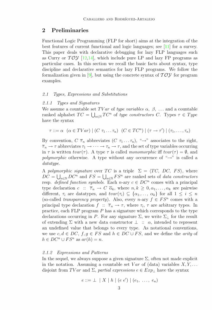
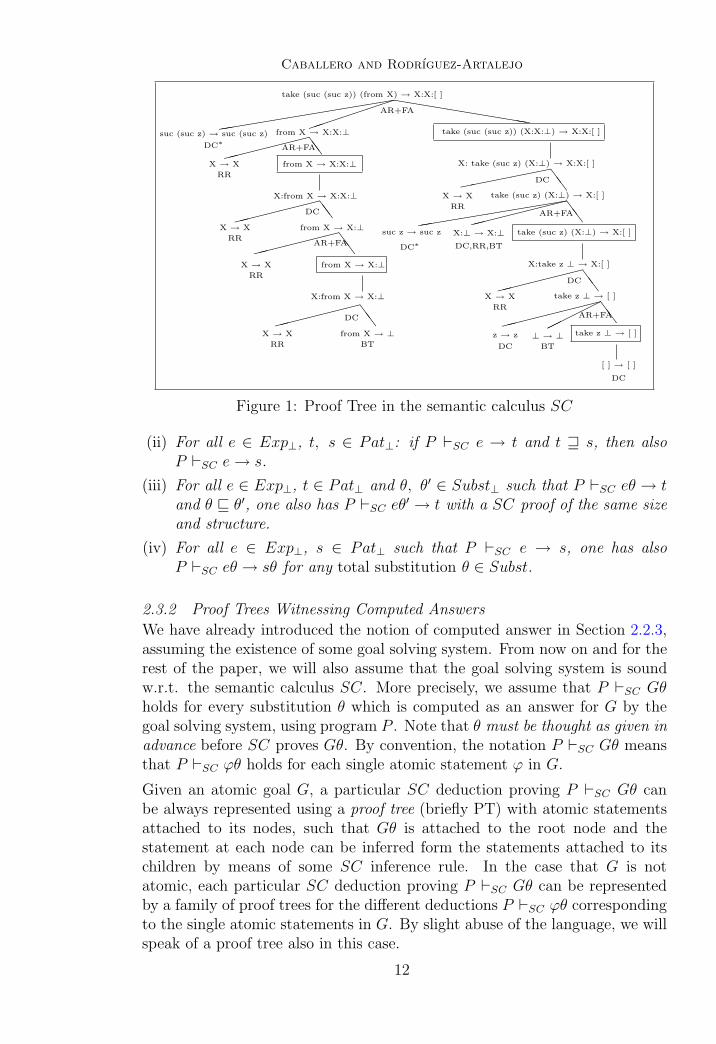
Figure 1: Proof Tree in the semantic calculus SC
(ii) For all e ∈ Exp⊥, t, s ∈ Pat⊥: if P `SC e → t and t w s, then alsoP `SC e→ s.
(iii) For all e ∈ Exp⊥, t ∈ Pat⊥ and θ, θ′ ∈ Subst⊥ such that P `SC eθ → tand θ v θ′, one also has P `SC eθ′ → t with a SC proof of the same sizeand structure.
(iv) For all e ∈ Exp⊥, s ∈ Pat⊥ such that P `SC e → s, one has alsoP `SC eθ → sθ for any total substitution θ ∈ Subst.
2.3.2 Proof Trees Witnessing Computed Answers
We have already introduced the notion of computed answer in Section 2.2.3,assuming the existence of some goal solving system. From now on and for therest of the paper, we will also assume that the goal solving system is soundw.r.t. the semantic calculus SC. More precisely, we assume that P `SC Gθholds for every substitution θ which is computed as an answer for G by thegoal solving system, using program P . Note that θ must be thought as given inadvance before SC proves Gθ. By convention, the notation P `SC Gθ meansthat P `SC ϕθ holds for each single atomic statement ϕ in G.
Given an atomic goal G, a particular SC deduction proving P `SC Gθ canbe always represented using a proof tree (briefly PT) with atomic statementsattached to its nodes, such that Gθ is attached to the root node and thestatement at each node can be inferred form the statements attached to itschildren by means of some SC inference rule. In the case that G is notatomic, each particular SC deduction proving P `SC Gθ can be representedby a family of proof trees for the different deductions P `SC ϕθ correspondingto the single atomic statements in G. By slight abuse of the language, we willspeak of a proof tree also in this case.
12
Caballero and Rodrıguez-Artalejo
take (suc (suc z)) (from X) → X:X:[ ]��������
from X → X:X:⊥
from X → X:⊥
XXXXXXXXtake (suc (suc z)) (X:X:⊥) → X:X:[ ]
take (suc z) (X:⊥) → X:[ ]
take z ⊥ → [ ]
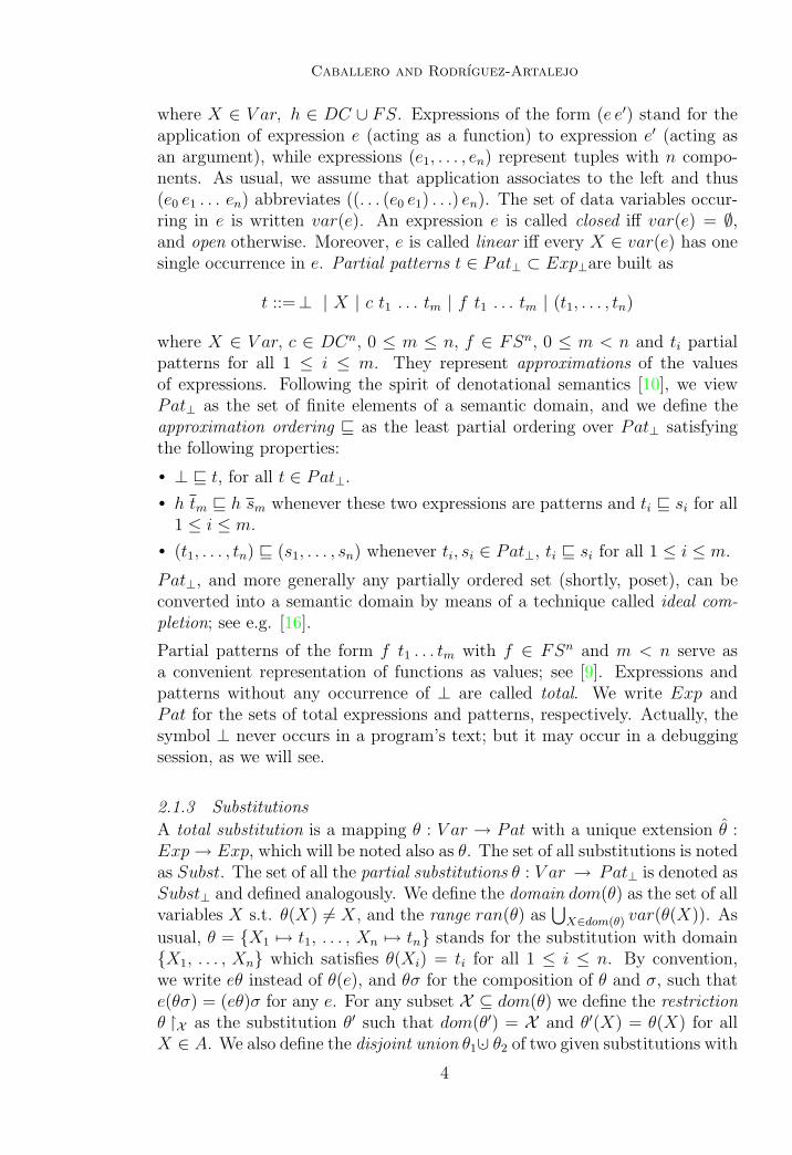
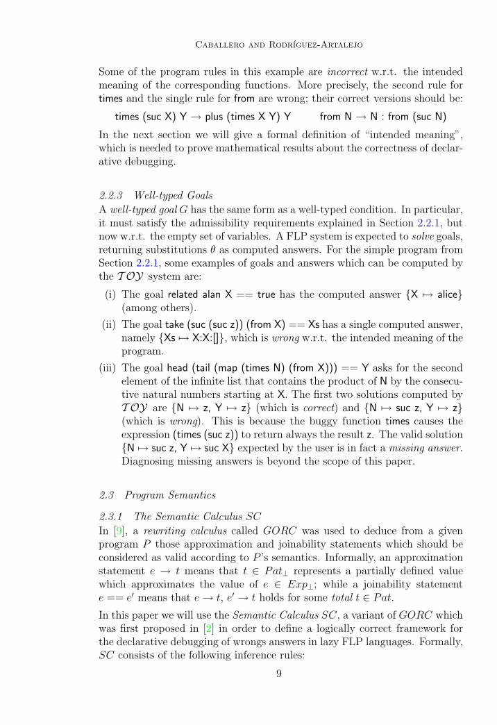
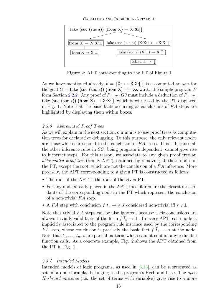
Figure 2: APT corresponding to the PT of Figure 1
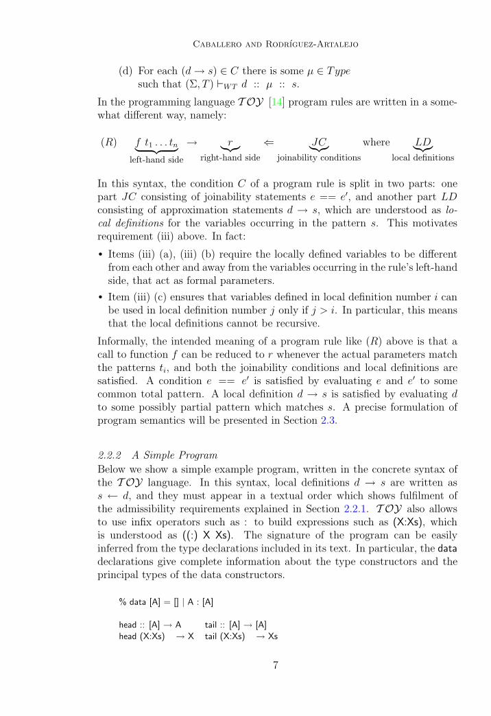
As we have mentioned already, θ = {Xs 7→ X:X:[]} is a computed answer forthe goal G = take (suc (suc z)) (from X) == Xs w.r.t. the simple program Pform Section 2.2.2. Any proof of P `SC Gθ must include a deduction of P `SCtake (suc (suc z)) (from X) → X:X:[], which is witnessed by the PT displayedin Fig. 1. Note that the basic facts occurring as conclusions of FA steps arehighlighted by displaying them within boxes.
2.3.3 Abbreviated Proof Trees
As we will explain in the next section, our aim is to use proof trees as computa-tion trees for declarative debugging. To this purpose, the only relevant nodesare those which correspond to the conclusion of FA steps. This is because allthe other inference rules in SC, being program independent, cannot give riseto incorrect steps. For this reason, we associate to any given proof tree anabbreviated proof tree (briefly APT), obtained by removing all those nodes ofthe PT, except the root, which are not the conclusion of a FA inference. Moreprecisely, the APT corresponding to a given PT is constructed as follows:
• The root of the APT is the root of the given PT.
• For any node already placed in the APT, its children are the closest descen-dants of the corresponding node in the PT which represent the conclusionof a non-trivial FA step.
• A FA step with conclusion f tn → s is considered non-trivial iff s 6=⊥.
Note that trivial FA steps can be also ignored, because their conclusions arealways trivially valid facts of the form f tn → ⊥. In every APT, each node isimplicitly associated to the program rule instance used by the correspondingFA step, whose conclusion is precisely the basic fact f tn → s at the node.Note that t1, . . . , tn, s are partial patterns which cannot contain any reduciblefunction calls. As a concrete example, Fig. 2 shows the APT obtained fromthe PT in Fig. 1.
2.3.4 Intended Models
Intended models of logic programs, as used in [6,13], can be represented assets of atomic formulas belonging to the program’s Herbrand base. The openHerbrand universe (i.e. the set of terms with variables) gives rise to a more
13
Caballero and Rodrıguez-Artalejo
informative semantics [5]. In our FLP setting, a natural analogous to the openHerbrand universe is the set Pat⊥ of all the partial patterns, equipped withthe approximation ordering v. Similarly, a natural analogous to the openHerbrand base is the collection of all the basic facts f tn → s. Therefore,we can define a Herbrand interpretation as a set I of basic facts fulfilling thefollowing three requirements for all f ∈ FSn and arbitrary partial patternst, tn:
(i) (f tn →⊥) ∈ I.
(ii) If (f tn → s) ∈ I, ti v t′i, s w s′ then also (f t′n → s′) ∈ I.
(iii) if (f tn → s) ∈ I, and θ is total substitution, then (f tn → s)θ ∈ I.
This definition of Herbrand interpretation is simpler than the one in [9], wherea more general notion of interpretation (under the name algebra) is presented.The trade-off for this simpler presentation is to exclude non-Herbrand inter-pretations from our consideration. In our debugging scheme we will assumethat the intended model of a program is a Herbrand interpretation I. Her-brand interpretations can be ordered by set inclusion.
A logically correct program P should conform to its intended interpretationI. In order to formalize this idea, we need some definitions. First, we saythat a given approximation or joinability statement ϕ is valid in the Herbrandinterpretation I iff ϕ can be proved in the calculus SCI consisting of the SCrules BT , RR, DC and JN together with the inference rule FAI below:
FAI e1 → t1 . . . en → tn s ak → t t pattern, t 6=⊥, s pattern
f en ak → t (f tn → s) ∈ I
For instance, assuming the natural intended model I for the simple programfrom Section 2.2.2, the following statements are valid in I:
(i) from X → X:suc X:⊥(ii) take (suc (suc z)) (from X) → X:suc X:[]
(iii) ancestor alan == ancestor alice
The first of these statements even belongs to I. In general, for every basicfact f tn → s, it can be proved that f tn → s is valid in I iff (f tn → s) ∈ I.
Next we define the denotation of expressions and the notion of model of agiven program:
• The denotation of e is the set [[e]]I = {s ∈ Pat⊥ | e→ s valid in I}.• I is a model of P (I |= P ) iff every program rule in P is valid in I.
• A program rule l → r ⇐ C is valid in I ( I |= l → r ⇐ C) iff for anysubstitution θ ∈ Subst⊥, I satisfies the rule instance lθ → rθ ⇐ Cθ.
• I satisfies a rule instance l′ → r′ ⇐ C ′ iff either I does not satisfy C ′ orelse [[l′]]I ⊇ [[r′]]I .
14
Caballero and Rodrıguez-Artalejo
• I satisfies an instantiated condition C ′ = ϕ1, . . . ϕk iff for i = 1 . . . k, Isatisfies ϕi.
• I satisfies d′ → s′ ∈ C ′, iff [[d′]]I ⊇ [[s′]]I . It can be shown that [[d′]]I ⊇ [[s′]]I
iff s′ ∈ [[d′]]I .
• I satisfies l′ == r′ ∈ C ′, iff [[l′]]I ∩ [[r′]]I ∩ Pat 6= ∅.The fundamental relationship between programs and models is stated in thefollowing result, which is proved in [9] for a notion of model more generalthan Herbrand models. A proof for the present formulation can be found inAppendix A.
Theorem 2.2 Let P be a program and ϕ any approximation or joinabilitystatement. Then:(a) If P `SC ϕ then ϕ is valid in any Herbrand model of P .(b) MP = {f tn → s | P `SC f tn → s} is the least Herbrand model of Pw.r.t. the inclusion ordering.(c) If ϕ is valid in MP then P `SC ϕ.
Putting together the previous theorem and the assumed soundness of the goalsolving system w.r.t. SC, we immediately obtain:
Proposition 2.3 Assume a program P and a computed answer θ for a goalG, such that Gθ is not valid in the Herbrand interpretation I. Then, theremust be some program rule in P which is not valid in I.
This proposition predicts the existence of at least one wrong program rulewhenever a wrong computed answer is observed. Here, wrong must be under-stood in the precise sense of being not valid in the intended model. In the caseof our simple program P , θ = {Xs 7→ X:X:[]} is a wrong computed answer forthe goal G = take (suc (suc z)) (from X) == Xs, because Gθ is not valid in theintended model. By Proposition 2.3, some wrong rule in P must be responsi-ble for the wrong answer. Indeed, the program rule defining the function fromis wrong.
Whenever a program rule l → r ⇐ C is not valid in the intended modelI, there must be some substitution θ ∈ Subst⊥ such that the rule instancelθ → rθ ⇐ Cθ is not satisfied by I, which means that
(i) ϕθ is valid in I for all ϕ ∈ C.
(ii) rθ → s is valid in I for some s ∈ Pat⊥ such that (lθ → s) /∈ I.
In our example, the incorrect instance of the rule defining from is the ruleitself. Indeed, N:from N → N:N:⊥ is valid in I, but (from N → N:N:⊥) /∈ I.This corresponds to item (ii) above, with N:N:⊥ acting as s.
For the purposes of practical debugging, Proposition 2.3 must be refined toyield an effective method which can be used to find an incorrect instance ofa program rule, starting from the observation of a wrong computed answer.
15
Caballero and Rodrıguez-Artalejo
In the next section, we show that this can be achieved by using a declarativedebugging scheme with APTs acting as computation trees. Effective methodsto implement this approach are investigated in the rest of the paper.
2.4 Declarative Debugging
2.4.1 A Generic Declarative Debugging Scheme
The debugging scheme proposed in [19] assumes that any terminated com-putation can be represented as a finite tree, called computation tree (brieflyCT). The root of this tree corresponds to the result of the main computation,and each node corresponds to the result of some intermediate subcomputa-tion. Moreover, it is assumed that the result at each node is determined bythe results of the children nodes. Therefore, every node can be seen as theoutcome of a single computation step. The debugger works by traversing agiven CT (so called CT navigation), looking for erroneous nodes. Differentkinds of programming paradigms and/or errors need different types of trees,as well as different notions of erroneous.
A sound debugger should only report bugs that really correspond to wrongcomputation steps. This consideration leads to ignore erroneous nodes whichhave some erroneous children, since they do not necessarily correspond towrong computation steps. Following the terminology of [19], an erroneousnode with no erroneous children is called a buggy node. In order to avoidunsoundness, the debugging scheme looks only for buggy nodes, asking ques-tions to an oracle (generally the user) in order to determine which nodes areerroneous. The following easy result is proved in [19]:
Proposition 2.4 A finite computation tree has an erroneous node iff it hasa buggy node. In particular, a finite computation tree whose root node iserroneous has some buggy node.
This provides a ‘weak’ notion of completeness for the debugging scheme thatis satisfactory in practice. Usually, actual debuggers look only for a topmostbuggy node in a computation tree whose root is erroneous. Multiple bugs canbe found by reiterated application of the debugger.
2.4.2 Debugging with APTs is Logically Correct
Our debugging system is based on the declarative debugging scheme just re-called. We assume well-typed FLP programs and goals, as described in Section2.2. We also suppose an intended model for each program, represented as aset of basic facts, as explained in Section 2.3.4. Computations are performedby a goal solving system which must be sound w.r.t. the semantic calculus SCfrom Section 2.3.1. Whenever a computation obtains an answer substitution θfor a goal G using program P , we assume that an APT witnessing P `SC Gθis used as computation tree. An APT node is considered erroneous iff the
16
Caballero and Rodrıguez-Artalejo
statement attached to it (which is always a basic fact, except perhaps for theroot) is not valid in the intended model.
The next theorem guarantees the logical correctness of declarative debuggingwith APTs:
Theorem 2.5 Assume a wrong computed answer θ, computed for the goal Gusing program P , such that Gθ is not valid in the intended model. Considerany APT witnessing P `SC Gθ, which must exist due to soundness of thegoal solving system w.r.t. SC. Then, declarative debugging using the APT ascomputation tree has the following two properties:
(a) Completeness: navigating the APT will find a buggy node.
(b) Soundness: every buggy node in the APT points to an instance of aprogram rule which is incorrect w.r.t. the intended model.
Proof.Item (a) follows immediately from Proposition 2.4, provided that the searchstrategy used to navigate the tree does not miss existing buggy nodes. To proveitem (b), assume that the intended model is I, the APT is apt, and the PTwhich has been abbreviated to obtain apt is pt. Now consider any given buggynode in apt. The corresponding node in pt must contain a basic fact f tn → swhich is not valid in I and has been inferred as the conclusion of a FA inferencestep using some instance of a program rule, say (f tn → r ⇐ C) ∈ [P ]⊥.Therefore, the children of f tn → s in pt correspond to the statement r → sand all the statements in C. In apt, the children of f tn → s are not necessarilythese; but since apt has been built as the abbreviated form of pt, it happensthat r → s and C can be inferred from the children of f tn → s in apt bymeans of SC inferences which are different from FA and therefore correct inevery Herbrand interpretation. Moreover, all the children of f tn → s in aptare valid in I, because they are the children of a buggy node. With this wecan conclude that C and r → s are valid in I, while f tn → s is not; whichmeans that the program rule instance (f tn → r ⇐ C) ∈ [P ]⊥ is incorrect inI. 2
This theorem provides an effective version of Proposition 2.3 as well as alogical interpretation of computation trees. To the best of our knowledge, thisis missing in other related approaches to declarative debugging of lazy FP andFLP programs [21,22,23,27,18,20,25].
As a concrete example, consider again the PT shown in Fig. 1 and the cor-responding APT shown in Fig. 2. As we have said before, PT witnesses thecomputation of the wrong answer θ = {Xs 7→ X:X:[]} for the goal
G = take (suc (suc z)) (fromX) == Xs
using the simple program from Section 2.2.2 5 . In Fig. 2, the statements at
5 Strictly speaking, a witnessing PT for this computation should have the joinability state-
17
Caballero and Rodrıguez-Artalejo
erroneous nodes are displayed in bold letters, and the only buggy node appearssurrounded by a double box. In this case, the reasoning of Theorem 2.5 leadsto the incorrect program rule instance used by the FA step at the buggy node,which is from N → N:from N.
In a previous work [2] we have presented a method to extract the APT whichwitnesses a particular computation from a formal representation of the com-putation in a lazy narrowing calculus. This theoretical result depends on aparticular formalization of narrowing, and does not provide a direct way toimplement a debugging tool for existing FLP systems. In the rest of this pa-per we propose more effective methods for the generation and navigation ofAPTs, which allow to implement a working debugging tool.
3 Problems and Contributions
In this short section we summarize the main contributions of this paper to thetwo stages of declarative debugging, namely CT generation and CT navigation.
3.1 CT Generation
In the context of lazy FP and FLP, two main ways of constructing CT’s havebeen proposed. The program transformation approach [22,20,25] gives riseto transformed programs whose functions return CTs along with the origi-nally expected results. The abstract machine approach [21,22,23,27] requireslower level modifications of the language implementation. Although the sec-ond approach can result in a better performance, we have adopted the firstone because we find it more portable and better suited to a formal correct-ness analysis. With respect to other papers based in the transformationalapproach, we present two main contributions, described below.
3.1.1 Curried Functions
Roughly, all transformational approaches transform the functions defined inthe source program to return pairs (res, ct) consisting of a computed resultand a CT. From the viewpoint of types, the transformation of a n-ary functionf ∈ FSn looks as follows:
f :: τ1 → · · · → τn → τ ⇒ fT :: τT1 → · · · → τTn → (τT , cTree)
where cTree is a datatype for representing CTs, and τTi resp. τT are suitabletransformations of the types τi resp. τ . This type transformation amounts tothe identity in the case of datatypes (i.e., types with no occurrence of the typeconstructor “→”), but it becomes relevant in the case of higher-order (briefly,HO) types, whose translation involves the type cTree. For instance, the types
ment take (suc (suc z)) (from X) == X:X:[] at the root; but the PT from Fig. 1 representsthe interesting part of the deduction.
18
Caballero and Rodrıguez-Artalejo
of the functions plus, drop4 and map from the simple program in Section 2.2.2,whose respective arities are 2, 0 and 2, are translated as shown below. Thetype of drop4 has the form (τT , cT ree) because drop4 has been declared as anullary function, to be defined by parameterless program rules.
plus :: nat → nat → nat ⇒ plusT :: nat → nat → (nat, cTree)
drop4 :: [A] → [A] ⇒ drop4T :: ([A] → ([A], cTree),cTree)
map :: (A →B) → [A] → [B] ⇒ mapT :: (A → (B,cTree)) → [A] → ([B],cTree)
As pointed out in [20,25], this approach can lead to type errors when curriedfunctions are used to compute results which are taken as parameters by otherfunctions. For instance, (map drop4) is well-typed, but the naıve translation(mapT drop4T ) is ill-typed, because the type of drop4T does not match thetype expected by mapT for its first parameter. More generally, the type of theresult returned by fT when applied to m arguments depends on the relationbetween m and f ’s arity n. For example, (map (plus z)) and (map plus) areboth well-typed. However, when translating naıvely, (mapT (plusT z)) remainswell-typed, while (mapT plusT ) becomes ill-typed.
As a possible solution to this problem, the authors of [20] suggest to modifythe translation in such a way that a curried function of arity n > 0 alwaysreturns a result of type (τT , cTree) when applied to its first parameter. Thetype translation of the function plus following this idea yields plusT :: nat →(nat → (nat, cTree), cTree).
However, as noted in [20], such a transformation would cause transformedprograms to compute inefficiently, producing CTs with many useless nodes.Therefore, the authors of [20] wrote: ”An intermediate transformation whichonly handles currying when necessary is desirable. Whether this can be donewithout detailed analysis of the program is under investigation”.
Our program transformation solves this problem by translating a curried func-tion f of arity n, into n curried functions fT0 , . . . , f
Tn−2, f
T with respectivearities 1, 2, . . .n − 1, n, and suitable types. Function fTm (0 ≤ m ≤ n − 2)is used to translate occurrences of f applied to m parameters, while fT trans-lates occurrences of f applied to n − 1 parameters. For instance, (map plus)is transformed into (map T plus0
T ), using the auxiliary function plus0T :: nat
→ (nat → (nat,cTree), cTree). As we will see formally in Section 4, the appli-cation of a n-ary function f to n or more parameters must be translated withthe help of local definitions, a technique already used in [22,20,25].
We provide a similar solution to deal with partial application of curried dataconstructors, which can also cause type errors in the naıve approach (thinkof (twiceT suc), as an example). As far as we know, the difficulties with cur-ried constructors have not been addressed previously. Our approach certainlyincreases the number of functions in transformed programs, but the extra
19
Caballero and Rodrıguez-Artalejo
functions are used only when needed, and inefficient CTs with useless nodescan be avoided. A detailed specification of the transformation, dealing bothwith types and with program rules, is presented in Section 4.
3.1.2 Correctness Results
Our program transformation preserves polymorphic well-typing (module thetype transformation τ 7→ τT ) as well as the program semantics formalizedin Section 2.3. Under some minimal and natural assumptions about the goalsolving system, we also prove that translated programs compute APTs whichcan be used for logically correct declarative debugging, as we have seen inSection 2.4.2, Theorem 2.5.
These correctness results are presented in Section 4. To the best of our knowl-edge, previous related papers [22,20,25] give no correctness proof for the pro-gram transformation. The author of [25], who is aware of the problem, justrelies on intuition for the semantic correctness. He mentions the need of aformalized semantics for a rigorous proof. As for type correctness, it is closelyrelated to the treatment of curried functions, which was deficient in previousapproaches.
3.2 CT Navigation
In order to be a really practical tool, a declarative debugger should keep thenumber of questions asked to the oracle as small as possible. Our debuggeruses a decidable and semantically correct entailment between basic facts tomaintain a consistent and non-redundant store of facts known from previouslyanswered questions. Redundant questions whose answer is entailed by storedfacts can be avoided. In Section 5 we define the entailment relation, provingits decidability and discussing its use during CT navigation.
4 Generation of CTs by Program Transformation
In this section we present the program transformation used by our debuggerand we prove its correctness. Roughly, a program P is converted into a newprogram P T , where function calls return the same results P would return,but paired with CTs. Formally, P T is obtained by transforming the signatureΣ of P into a new signature ΣT , introducing definitions for certain auxiliaryfunctions, and transforming the function definitions included in P . Let usconsider these issues one by one.
4.1 Representing Computation Trees
A transformed program always includes the constructors of the datatype cTree,used to represent CTs and defined as follows:
20
Caballero and Rodrıguez-Artalejo
data cTree = void | cNode funId [arg] res rule [cTree]
type arg, res = pVal
type funId, pVal, rule = string
A CT of the form (cNode f ts s rl cts) corresponds to a call to the functionf with arguments ts and result s, where rl indicates the function rule used toevaluate the call, and the list cts consists of the children CTs corresponding toall the function calls (in the local definitions, right-hand side and conditions ofrl) whose activation was needed in order to obtain s. Due to lazy evaluation,the main computation may demand only partial approximations of the resultsof intermediate computations. Therefore, ts and s stand for possibly partialvalues, represented as partial patterns; and (f ts → s) represents the basicfact whose validity will be asked to the oracle during debugging, as explainedin Section 2.4. As for void, it represents an empty CT, returned by calls tofunctions which are trusted to be correct (in particular, data constructors andthe auxiliary functions introduced by the translation). Finally, the definitionof arg, res, funId, pVal and rule as synonyms of the type of character strings isjust a simple representation; other choices are possible. In fact, our currentprototype debugger uses more structured representations instead of strings. Inparticular, values of type rule in our debugging system represent instances ofprogram rules, so that the wrong program rule instances associated to buggynodes can be presented to the user.
4.2 Transforming Program Signatures
For every n-ary function f :: τ1 → . . . → τn → τ occurring in P , P T mustinclude an (m+ 1)-ary auxiliary function fTm for each 0 ≤ m < n− 1, as wellas an n-ary function fT , with principal types:
fTm :: τT1 → . . .→ τTm+1 → ((τm+2 → . . .→ τn → τ)T , cTree)
fT :: τT1 → . . .→ τTn → (τT , cTree)
Similarly, for each n-ary data constructor c :: τ1 → . . .→ τn → τ occurring inP , P T must keep c with the same principal type, and include new (m+1)-aryauxiliary functions cTm (0 ≤ m < n), with principal types:
cTm :: τT1 → . . .→ τTm+1 → ((τm+2 → . . .→ τn → τ)T , cTree)
Note that cTm are not data constructors in the translated signature. Definingrules for them will be presented below. The principal types declared above forthe function symbols in the transformed signature depend on a type transfor-mation. Any type τ in P ’s signature is transformed into another type τT inP T ’s signature, which is recursively defined as follows:
21
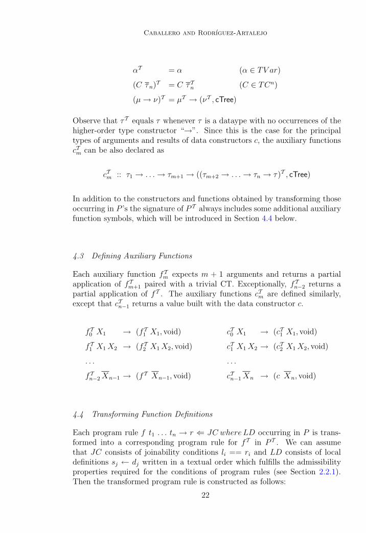
Caballero and Rodrıguez-Artalejo
αT = α (α ∈ TV ar)
(C τn)T = C τTn (C ∈ TCn)
(µ→ ν)T = µT → (νT , cTree)
Observe that τT equals τ whenever τ is a dataype with no occurrences of thehigher-order type constructor “→”. Since this is the case for the principaltypes of arguments and results of data constructors c, the auxiliary functionscTm can be also declared as
cTm :: τ1 → . . .→ τm+1 → ((τm+2 → . . .→ τn → τ)T , cTree)
In addition to the constructors and functions obtained by transforming thoseoccurring in P ’s the signature of P T always includes some additional auxiliaryfunction symbols, which will be introduced in Section 4.4 below.
4.3 Defining Auxiliary Functions
Each auxiliary function fTm expects m + 1 arguments and returns a partialapplication of fTm+1 paired with a trivial CT. Exceptionally, fTn−2 returns apartial application of fT . The auxiliary functions cTm are defined similarly,except that cTn−1 returns a value built with the data constructor c.
fT0 X1 → (fT1 X1, void) cT0 X1 → (cT1 X1, void)
fT1 X1X2 → (fT2 X1X2, void) cT1 X1X2 → (cT2 X1X2, void)
. . . . . .
fTn−2Xn−1 → (fT Xn−1, void) cTn−1Xn → (c Xn, void)
4.4 Transforming Function Definitions
Each program rule f t1 . . . tn → r ⇐ JC whereLD occurring in P is trans-formed into a corresponding program rule for fT in P T . We can assumethat JC consists of joinability conditions li == ri and LD consists of localdefinitions sj ← dj written in a textual order which fulfills the admissibilityproperties required for the conditions of program rules (see Section 2.2.1).Then the transformed program rule is constructed as follows:
22
Caballero and Rodrıguez-Artalejo
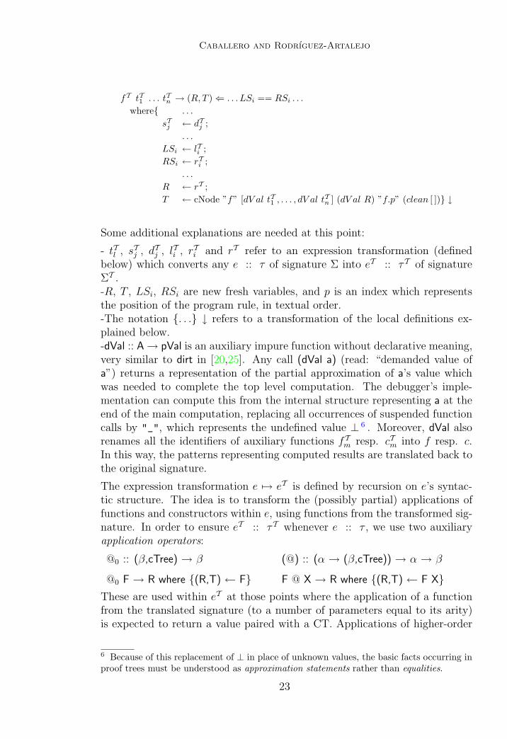
fT tT1 . . . tTn → (R, T )⇐ . . . LSi == RSi . . .
where{ . . .
sTj ← dTj ;. . .
LSi ← lTi ;RSi ← rTi ;
. . .
R ← rT ;T ← cNode ”f” [dV al tT1 , . . . , dV al t
Tn ] (dV al R) ”f.p” (clean [ ])} ↓
Some additional explanations are needed at this point:
- tTl , sTj , dTj , lTi , rTi and rT refer to an expression transformation (definedbelow) which converts any e :: τ of signature Σ into eT :: τT of signatureΣT .-R, T , LSi, RSi are new fresh variables, and p is an index which representsthe position of the program rule, in textual order.-The notation {. . .} ↓ refers to a transformation of the local definitions ex-plained below.-dVal :: A→ pVal is an auxiliary impure function without declarative meaning,very similar to dirt in [20,25]. Any call (dVal a) (read: “demanded value ofa”) returns a representation of the partial approximation of a’s value whichwas needed to complete the top level computation. The debugger’s imple-mentation can compute this from the internal structure representing a at theend of the main computation, replacing all occurrences of suspended functioncalls by "_", which represents the undefined value ⊥ 6 . Moreover, dVal alsorenames all the identifiers of auxiliary functions fTm resp. cTm into f resp. c.In this way, the patterns representing computed results are translated back tothe original signature.
The expression transformation e 7→ eT is defined by recursion on e’s syntac-tic structure. The idea is to transform the (possibly partial) applications offunctions and constructors within e, using functions from the transformed sig-nature. In order to ensure eT :: τT whenever e :: τ , we use two auxiliaryapplication operators:
@0 :: (β,cTree) → β
@0 F → R where {(R,T) ← F}
(@) :: (α → (β,cTree)) → α → β
F @ X → R where {(R,T) ← F X}These are used within eT at those points where the application of a functionfrom the translated signature (to a number of parameters equal to its arity)is expected to return a value paired with a CT. Applications of higher-order
6 Because of this replacement of ⊥ in place of unknown values, the basic facts occurring inproof trees must be understood as approximation statements rather than equalities.
23
Caballero and Rodrıguez-Artalejo
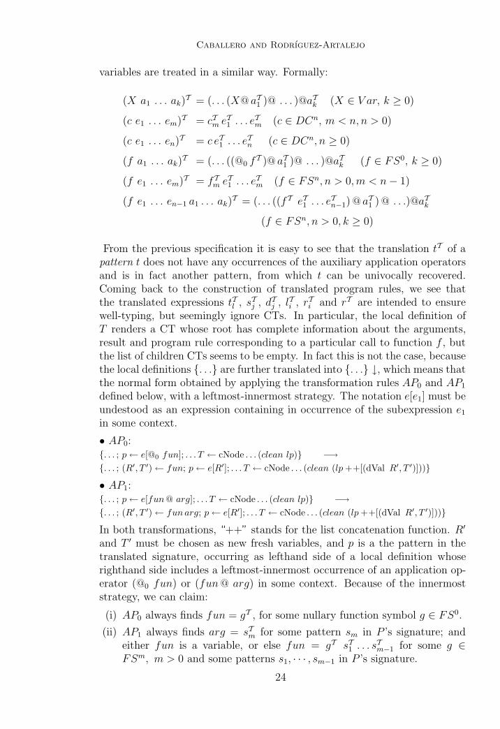
variables are treated in a similar way. Formally:
(X a1 . . . ak)T = (. . . (X@ aT1 )@ . . . )@aTk (X ∈ V ar, k ≥ 0)
(c e1 . . . em)T = cTm eT1 . . . e
Tm (c ∈ DCn, m < n, n > 0)
(c e1 . . . en)T = c eT1 . . . eTn (c ∈ DCn, n ≥ 0)
(f a1 . . . ak)T = (. . . ((@0 f
T )@ aT1 )@ . . . )@aTk (f ∈ FS0, k ≥ 0)
(f e1 . . . em)T = fTm eT1 . . . e
Tm (f ∈ FSn, n > 0,m < n− 1)
(f e1 . . . en−1 a1 . . . ak)T = (. . . ((fT eT1 . . . e
Tn−1) @ aT1 ) @ . . .)@aTk
(f ∈ FSn, n > 0, k ≥ 0)
From the previous specification it is easy to see that the translation tT of apattern t does not have any occurrences of the auxiliary application operatorsand is in fact another pattern, from which t can be univocally recovered.Coming back to the construction of translated program rules, we see thatthe translated expressions tTl , sTj , dTj , lTi , rTi and rT are intended to ensurewell-typing, but seemingly ignore CTs. In particular, the local definition ofT renders a CT whose root has complete information about the arguments,result and program rule corresponding to a particular call to function f , butthe list of children CTs seems to be empty. In fact this is not the case, becausethe local definitions {. . .} are further translated into {. . .} ↓, which means thatthe normal form obtained by applying the transformation rules AP0 and AP1
defined below, with a leftmost-innermost strategy. The notation e[e1] must beundestood as an expression containing in occurrence of the subexpression e1in some context.
• AP0:{. . . ; p← e[@0 fun]; . . . T ← cNode . . . (clean lp)} −→{. . . ; (R′, T ′)← fun; p← e[R′]; . . . T ← cNode . . . (clean (lp++[(dVal R′, T ′)]))}
• AP1:{. . . ; p← e[fun@ arg]; . . . T ← cNode . . . (clean lp)} −→{. . . ; (R′, T ′)← fun arg; p← e[R′]; . . . T ← cNode . . . (clean (lp++[(dVal R′, T ′)]))}
In both transformations, “++” stands for the list concatenation function. R′
and T ′ must be chosen as new fresh variables, and p is a the pattern in thetranslated signature, occurring as lefthand side of a local definition whoserighthand side includes a leftmost-innermost occurrence of an application op-erator (@0 fun) or (fun@ arg) in some context. Because of the innermoststrategy, we can claim:
(i) AP0 always finds fun = gT , for some nullary function symbol g ∈ FS0.
(ii) AP1 always finds arg = sTm for some pattern sm in P ’s signature; andeither fun is a variable, or else fun = gT sT1 . . . s
Tm−1 for some g ∈
FSm, m > 0 and some patterns s1, · · · , sm−1 in P ’s signature.
24
Caballero and Rodrıguez-Artalejo
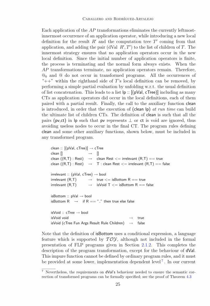
Each application of the AP transformations eliminates the currently leftmost-innermost occurrence of an application operator, while introducing a new localdefinition for the result R′ and the computation tree T ′ coming from thatapplication, and adding the pair (dVal R′, T ′) to the list of children of T . Theinnermost strategy ensures that no application operators occur in the newlocal definition. Since the initial number of application operators is finite,the process is terminating and the normal form always exists. When theAP transformations terminate, no application operators remain. Therefore,@0 and @ do not occur in transformed programs. All the occurrences of“++” within the righthand side of T ’s local definition can be removed, byperforming a simple partial evaluation by unfolding w.r.t. the usual definitionof list concatenation. This leads to a list lp :: [(pVal, cTree)] including as manyCTs as application operators did occur in the local definitions, each of thempaired with a partial result. Finally, the call to the auxiliary function cleanis introduced, in order that the execution of (clean lp) at run time can buildthe ultimate list of children CTs. The definition of clean is such that all thepairs (pv,ct) in lp such that pv represents ⊥ or ct is void are ignored, thusavoiding useless nodes to occur in the final CT. The program rules definingclean and some other auxiliary functions, shown below, must be included inany transformed program.
clean :: [(pVal, cTree)] → cTree
clean [] → []
clean ((R,T) : Rest) → clean Rest <= irrelevant (R,T) == true
clean ((R,T) : Rest) → T : clean Rest <= irrelevant (R,T) == false
irrelevant :: (pVal, cTree) → bool
irrelevant (R,T) → true <= isBottom R == true
irrelevant (R,T) → isVoid T <= isBottom R == false
isBottom :: pVal → bool
isBottom R → if R == ” ” then true else false
isVoid :: cTree → bool
isVoid void → true
isVoid (cTree Fun Args Result Rule Children) → false
Note that the definition of isBottom uses a conditional expression, a languagefeature which is supported by T OY, although not included in the formalpresentation of FLP programs given in Section 2.1.2. This completes thedescription of the program transformation, except for the behaviour of dVal.This impure function cannot be defined by ordinary program rules, and it mustbe provided at some lower, implementation dependent level 7 . In our current
7 Nevertheless, the requirements on dVal’s behaviour needed to ensure the semantic cor-rection of transformed programs can be formally specified; see the proof of Theorem 4.3
25
Caballero and Rodrıguez-Artalejo
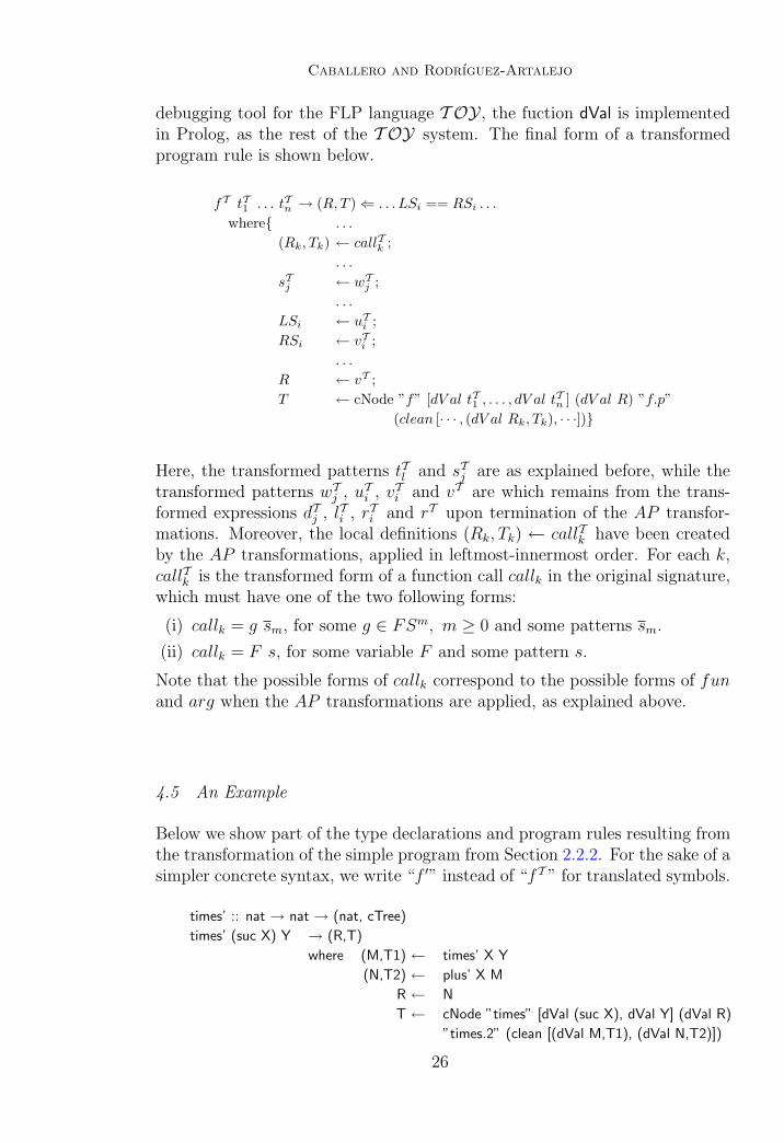
debugging tool for the FLP language T OY, the fuction dVal is implementedin Prolog, as the rest of the T OY system. The final form of a transformedprogram rule is shown below.
fT tT1 . . . tTn → (R, T )⇐ . . . LSi == RSi . . .
where{ . . .
(Rk, Tk) ← callTk ;. . .
sTj ← wTj ;. . .
LSi ← uTi ;RSi ← vTi ;
. . .
R ← vT ;T ← cNode ”f” [dV al tT1 , . . . , dV al t
Tn ] (dV al R) ”f.p”
(clean [· · · , (dV al Rk, Tk), · · ·])}
Here, the transformed patterns tTl and sTj are as explained before, while thetransformed patterns wTj , uTi , vTi and vT are which remains from the trans-formed expressions dTj , lTi , rTi and rT upon termination of the AP transfor-mations. Moreover, the local definitions (Rk, Tk) ← callTk have been createdby the AP transformations, applied in leftmost-innermost order. For each k,callTk is the transformed form of a function call callk in the original signature,which must have one of the two following forms:
(i) callk = g sm, for some g ∈ FSm, m ≥ 0 and some patterns sm.
(ii) callk = F s, for some variable F and some pattern s.
Note that the possible forms of callk correspond to the possible forms of funand arg when the AP transformations are applied, as explained above.
4.5 An Example
Below we show part of the type declarations and program rules resulting fromthe transformation of the simple program from Section 2.2.2. For the sake of asimpler concrete syntax, we write “f ′” instead of “fT ” for translated symbols.
times’ :: nat → nat → (nat, cTree)
times’ (suc X) Y → (R,T)
where (M,T1) ← times’ X Y
(N,T2) ← plus’ X M
R ← N
T ← cNode ”times” [dVal (suc X), dVal Y] (dVal R)
”times.2” (clean [(dVal M,T1), (dVal N,T2)])
26
Caballero and Rodrıguez-Artalejo
twice’ :: (A → (A, cTree)) → A → (A, cTree)
twice’ F X → (R,T)
where (Y,T1) ← F X
(Z,T2) ← F Y
R ← Z
T ← cNode ”twice” [dVal F, dVal X] (dVal R)
”twice.1” (clean [(dVal Y,T1), (dVal Z,T2)])
drop4’ :: ([A] → ([A], cTree), cTree)
drop4’ → (R,T)
where (F,T1) ← twice’ twice0’ tail’
R ← F
T ← cNode ”drop4” [] (dVal R)
”drop4.1” (clean [(dVal F,T1)]))
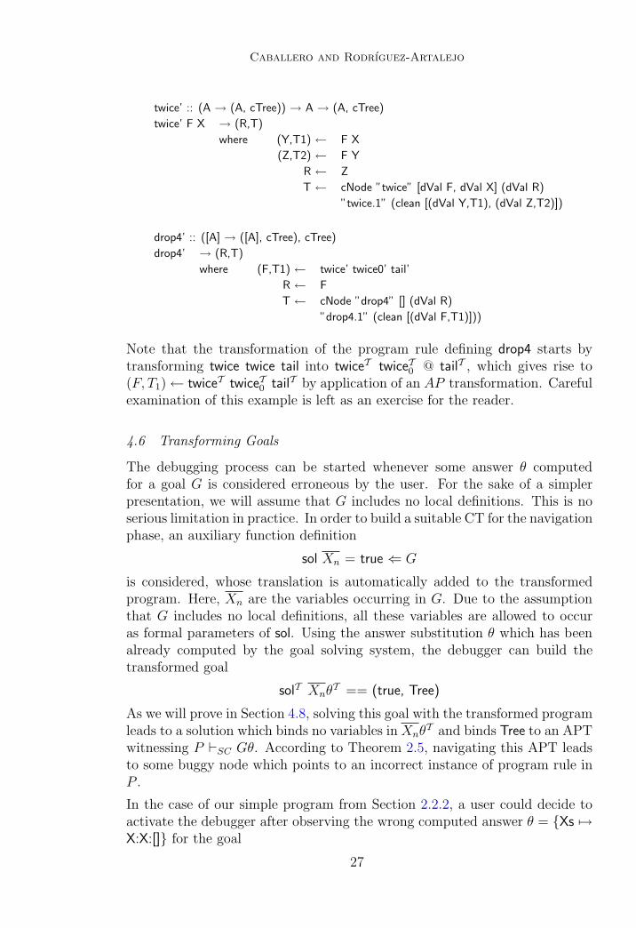
Note that the transformation of the program rule defining drop4 starts bytransforming twice twice tail into twiceT twiceT0 @ tailT , which gives rise to(F, T1)← twiceT twiceT0 tailT by application of an AP transformation. Carefulexamination of this example is left as an exercise for the reader.
4.6 Transforming Goals
The debugging process can be started whenever some answer θ computedfor a goal G is considered erroneous by the user. For the sake of a simplerpresentation, we will assume that G includes no local definitions. This is noserious limitation in practice. In order to build a suitable CT for the navigationphase, an auxiliary function definition
sol Xn = true ⇐ G
is considered, whose translation is automatically added to the transformedprogram. Here, Xn are the variables occurring in G. Due to the assumptionthat G includes no local definitions, all these variables are allowed to occuras formal parameters of sol. Using the answer substitution θ which has beenalready computed by the goal solving system, the debugger can build thetransformed goal
solT XnθT == (true, Tree)
As we will prove in Section 4.8, solving this goal with the transformed programleads to a solution which binds no variables in Xnθ
T and binds Tree to an APTwitnessing P `SC Gθ. According to Theorem 2.5, navigating this APT leadsto some buggy node which points to an incorrect instance of program rule inP .
In the case of our simple program from Section 2.2.2, a user could decide toactivate the debugger after observing the wrong computed answer θ = {Xs 7→X:X:[]} for the goal
27
Caballero and Rodrıguez-Artalejo
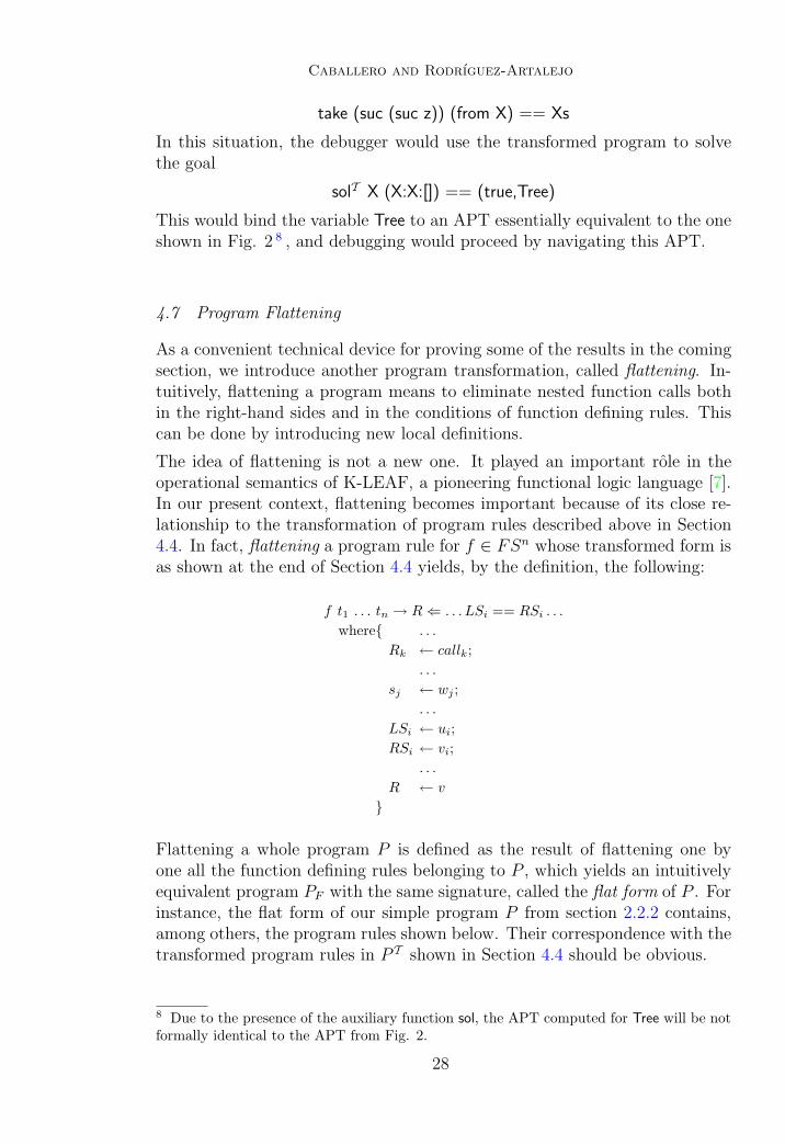
take (suc (suc z)) (from X) == Xs
In this situation, the debugger would use the transformed program to solvethe goal
solT X (X:X:[]) == (true,Tree)
This would bind the variable Tree to an APT essentially equivalent to the oneshown in Fig. 2 8 , and debugging would proceed by navigating this APT.
4.7 Program Flattening
As a convenient technical device for proving some of the results in the comingsection, we introduce another program transformation, called flattening. In-tuitively, flattening a program means to eliminate nested function calls bothin the right-hand sides and in the conditions of function defining rules. Thiscan be done by introducing new local definitions.
The idea of flattening is not a new one. It played an important role in theoperational semantics of K-LEAF, a pioneering functional logic language [7].In our present context, flattening becomes important because of its close re-lationship to the transformation of program rules described above in Section4.4. In fact, flattening a program rule for f ∈ FSn whose transformed form isas shown at the end of Section 4.4 yields, by the definition, the following:
f t1 . . . tn → R⇐ . . . LSi == RSi . . .
where{ . . .
Rk ← callk;. . .
sj ← wj ;. . .
LSi ← ui;RSi ← vi;
. . .
R ← v
}
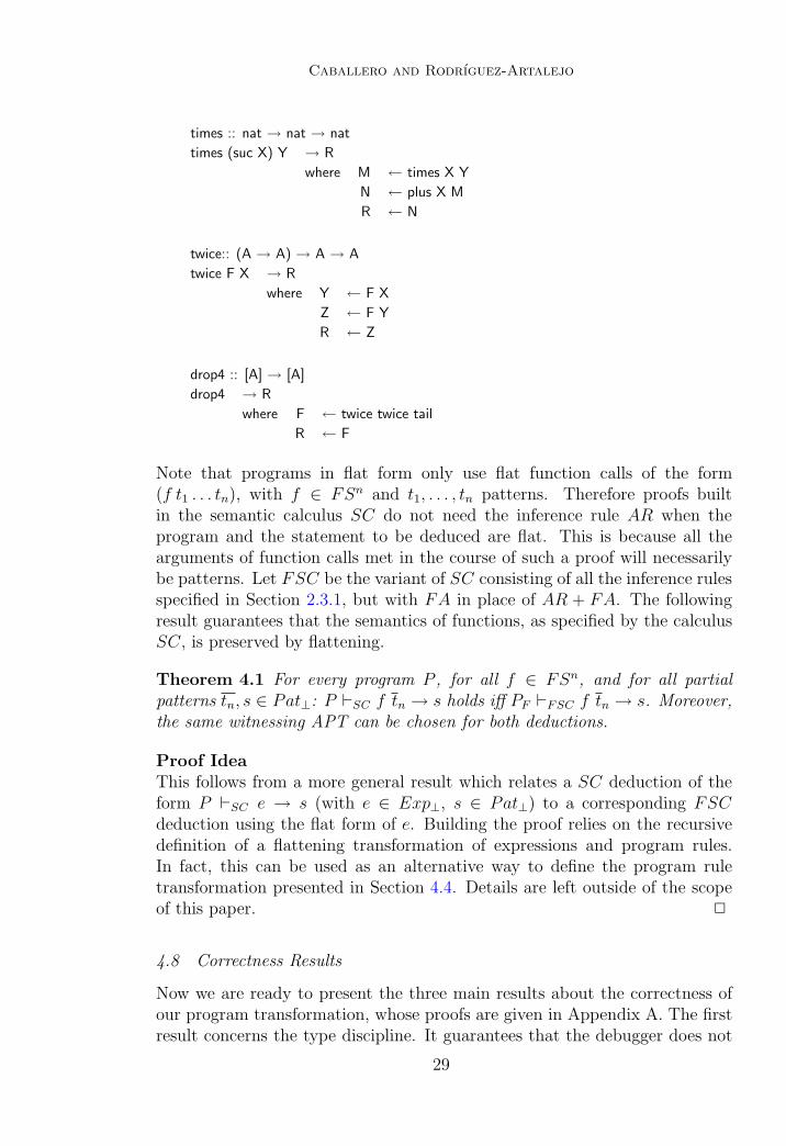
Flattening a whole program P is defined as the result of flattening one byone all the function defining rules belonging to P , which yields an intuitivelyequivalent program PF with the same signature, called the flat form of P . Forinstance, the flat form of our simple program P from section 2.2.2 contains,among others, the program rules shown below. Their correspondence with thetransformed program rules in P T shown in Section 4.4 should be obvious.
8 Due to the presence of the auxiliary function sol, the APT computed for Tree will be notformally identical to the APT from Fig. 2.
28
Caballero and Rodrıguez-Artalejo
times :: nat → nat → nat
times (suc X) Y → R
where M ← times X Y
N ← plus X M
R ← N
twice:: (A → A) → A → A
twice F X → R
where Y ← F X
Z ← F Y
R ← Z
drop4 :: [A] → [A]
drop4 → R
where F ← twice twice tail
R ← F
Note that programs in flat form only use flat function calls of the form(f t1 . . . tn), with f ∈ FSn and t1, . . . , tn patterns. Therefore proofs builtin the semantic calculus SC do not need the inference rule AR when theprogram and the statement to be deduced are flat. This is because all thearguments of function calls met in the course of such a proof will necessarilybe patterns. Let FSC be the variant of SC consisting of all the inference rulesspecified in Section 2.3.1, but with FA in place of AR + FA. The followingresult guarantees that the semantics of functions, as specified by the calculusSC, is preserved by flattening.
Theorem 4.1 For every program P , for all f ∈ FSn, and for all partialpatterns tn, s ∈ Pat⊥: P `SC f tn → s holds iff PF `FSC f tn → s. Moreover,the same witnessing APT can be chosen for both deductions.
Proof IdeaThis follows from a more general result which relates a SC deduction of theform P `SC e → s (with e ∈ Exp⊥, s ∈ Pat⊥) to a corresponding FSCdeduction using the flat form of e. Building the proof relies on the recursivedefinition of a flattening transformation of expressions and program rules.In fact, this can be used as an alternative way to define the program ruletransformation presented in Section 4.4. Details are left outside of the scopeof this paper. 2
4.8 Correctness Results
Now we are ready to present the three main results about the correctness ofour program transformation, whose proofs are given in Appendix A. The firstresult concerns the type discipline. It guarantees that the debugger does not
29
Caballero and Rodrıguez-Artalejo
need to perform any type checking/inference before entering the CT generationphase, which proceeds as explained in Section 4.6.
Theorem 4.2 The transformation P T of a well-typed program P is alwayswell-typed.
The second result says that the semantics of any transformed function fT ina transformed program P T is the same as the semantics of f in the originalprogram P , except that calls to fT also return APTs, represented as valuesof type cTree.
Theorem 4.3 Consider any n-ary function f and arbitrary partial patternstn, t in the signature of a program P .
(i) Assume P `SC f tn → t and let apt be a witnessing APT for thisdeduction. Then P T `FSCT fT tTn → (tT , ct), where ct :: cTree is a totalpattern which represents apt.
(ii) Assume P T `FSCT fT tTn → (tT , ct). Then P `SC f tn → t.
Proof Idea.Due to Theorem 4.1, the SC deduction P `SC f tn → t can be replacedby the FSC deduction PF `FSC f tn → t in the statement of the theorem.Intuitively, this makes the result plausible, due to the close correspondencebetween flat program rules and transformed program rules. The notationFSCT refers to a variant of the flat semantic calculus FSC, which mustbe used for deductions with transformed programs. FSCT consists of theinference rules of SC but with FA in place of AR+FA and with the additionof special metarules which formalize the behaviour of the impure functiondVal. Full details are given in Appendix A. 2
Our last result shows that the goal transformation described in Section 4.6 isindeed suitable to generate correct APTs. Before presenting the theorem, weformalize certain assumptions about the undelying goal solving system. Thetheorem holds for every goal solving system which satisfies these assumptions.
Definition 4.4
(a) A goal solving system GS is assumed to produce an ordered sequence ofcomputed answers θi for a given program P and a goal G. Each com-puted answer θi is assumed to be a substitution of patterns for variablesoccurring in G. We write G GS,P θ to indicate that θ is one of theanswers for G computed by GS with program P . Similarly, we writeG 1st
GS,P θ to indicate that θ is the first answer for G computed by GSusing program P .
(b) Given a goal solving system GS, we say(b.1) GS is stable iff for every program P and every goal G without local
30
Caballero and Rodrıguez-Artalejo
definitions: if G GS,P θ then sol Xnθ == true 1stGS,Psol
id, where
Psol = P ∪· {sol Xn → true⇐ G}, with a new n-ary function symbolsol and Xn = var(G).
(b.2) GS is sound iff for every program P and goal G, if G GS,P θ thenP `SC Gθ.
(b.3) GS is weakly complete iff for every program P , for any p :: τn → booland for all patterns tn in P ′s signature: If p tn == true 1st
GS,P id,and apt is the APT for P `SC p tn → true witnessing the previouscomputation (which exists by soundness) and P T FSCT pT tT n →(true, ct) where ct represents apt, then pT tT n == (true, T ) 1st
GS,PT
{T 7→ ct}.(b.4) GS is reasonable iff GS is stable, sound and weakly complete.
The items of the previous definition are intended as minimal requirements thatshould be fulfilled by goal solving systems based on lazy narrowing strategies.Weak completeness is a sensible assumption because of Theorem 4.3 (i), andstability can be guarenteed by treating all the variables occurring in Xnθ asconstants when solving a goal sol Xnθ == true.
We believe that the goal solving system underlying T OY [14] is reasonable inthe technical sense of Definition 4.4 but presently we do not intend to supportour belief by a mathematical proof. It would be a very hard task, as anyformal correctness proof for a complex software system.
Now we are in a position to state:
Theorem 4.5 Let G be a goal with variables Xn and without local defini-tions. Assume that θ has been computed as an answer for G using program P .Consider the program Psol obtained by adding to P the new auxiliary functiondefinition sol Xn = true⇐ G. If the goal solving system is reasonable, solvingthe transformed goal solT Xnθ
T == (true, Tree) with the transformed programP Tsol succeeds. Moreover, the first computed answer binds no variables in Xnθ
T
and binds Tree to an APT wittnessing P `SC Gθ.
A proof of this theorem can be found in Appendix A. Although the resultholds for any computed answer θ, its interest for debugging is restricted tothe case that θ is seen by the user as a wrong computed answer. In this case,the debugger can find an incorrect program rule by navigating the APT, asexplained in Section 4.6.
5 Navigating the CTs by Oracle Querying
In this Section we present a technique used by our debugger to avoid redundantquestions to the oracle during the navigation phase. We also present a simpleexample of debugging session. More examples can be found in Appendix B.
Once the CT associated to a wrong answer has been built (as described in
31
Caballero and Rodrıguez-Artalejo
Section 4.6), navigation performs a top-down traversal, asking the oracle aboutthe validity of the basic facts associated to the visited nodes (except for theroot, which is known to be erroneous in advance). For the sake of practicalusefulness, it is important to ensure that questions asked to the oracle are asfew and as simple as possible.
The second condition - simplicity - comes along with our choice of APTsas CTs, since basic facts are the minimal pieces of information needed tocharacterize the intended model of a program, as we have seen in Section2.3.4. To reduce the number of questions, the only possibility considered inrelated papers is to avoid asking repeated questions. As an improvement, wepresent an entailment relation between basic facts, and we show that it canbe used to avoid redundant questions which can be deduced from previousanswers.
Our notion of entailment is based on the approximation ordering v defined inSection 2.1.2. By definition, a basic fact f tn → t entails another basic factf sn → s (written as f tn → t � f sn → s) iff there is some total substitutionθ ∈ Subst such that
t1θ v s1, . . . , tnθ v sn, s v tθ
Due to Proposition 2.1 item (i), we can also write these conditions as:
s1 → t1θ, . . . , sn → tnθ, tθ → s
Entailment between basic fact can be decided by means of the next algorithm.
AlgorithmLet f tn → t and f sn → s be two basic facts which share no common variables.In order to decide whether f tn → t � f sn → s we define a system oftransformations, somewhat similar to those used in Martelli and Montanari’sunification algorithm. The transformations are applied to a multiset S ofapproximation statements a → b, with a, b ∈ Pat⊥, together with a set ofvariables W . Both are represented together in the form: S2W , which we willcall a configuration from now on.
We say that Sθ holds, with θ ∈ Subst, iff for all s→ t ∈ S, tθ v sθ. The set ofsolutions of a configuration S2W is defined as the set of total substitutionsover variables in W for which all the approximation statements in S do hold,i.e.: Sol(S2W ) = {θ ∈ Subst | dom(θ) ⊆W, ran(θ) ⊆ Pat, Sθ holds }.The purpose of the algorithm is to find some solution for the initial configura-tion S02W0 with S0 = s1 → t1, . . . , sn → tn, t→ s and W0 = var(f tn → t),i.e. we indicate that only variables in f tn → t can be instantiated. At eachstep of the algorithm a configuration Si2Wi is transformed into a new oneSi+12Wi+1 producing a substitution θi+1. This is done by applying some (non-deterministically) selected transformation rule to any (non-deterministically)
32
Caballero and Rodrıguez-Artalejo
selected element a→ b of Si. Such step can be represented as
a→ b, S︸ ︷︷ ︸
Si
2Wi `θi Si+12Wi+1
For the sake of simplicity, sometimes we will write a configuration Si2Wi asKi. The transformation rules are presented below.
Transformation RulesIn the following we assume X, Y ∈ V ar with X ∈ W ; ak, bk, t ∈ Pat⊥;s ∈ Pat; and h ∈ DC ∪ FS. Moreover, Xk represent new, fresh variables.
R1 Y → Y, S2W `id S2W
R2 t→⊥, S2W `id S2W
R3 h am → h bm, S2W `id . . . , ak → bk, . . . S2W
R4 s→ X, S2W `{X 7→s} S{X 7→ s}2WR5 X → Y, S2W `{X 7→Y } S{X 7→ Y }2WR6 X → h am, S2W `{X 7→h Xm} . . . , Xk → ak, . . . S{X 7→ h Xm}2W,Xm
The algorithm finishes when a configuration is reached s.t. no transformationcan be applied. Next theorem ensures that such configuration always exists,as well as its relationship with the entailment. The proof can be found inAppendix A.
Theorem 5.1 The algorithm described above always stops in some config-uration Sj2Wj which cannot be further transformed. Moreover, the initialentailment f tn → t � f sn → s holds iff Sj = ∅.
Now, the interest of the entailment for declarative debugging is justified bythe next result.
Theorem 5.2 Entailment between basic facts is a decidable preorder. More-over, any intended model given as a Herbrand interpretation I is closed underentailment, i.e. if f tn → t � f sn → s and (f tn → t) ∈ I then(f sn → s) ∈ I.
Proof.The fact that Herbrand interpretations are closed under entailment is a straight-forward consequence from the definition of the entailment relation and condi-tions (ii), (iii) in the definition of Herbrand interpretation (see Section 2.3.4).The definition of entailment also implies easily that � is a reflexive and transi-tive relation, and thus a preorder. In order to prove that � is decidable, let usconsider two arbitrary basic facts f tn → t, f sn → s and choose any renamingρ such that (f tn → t)ρ and f sn → s share no variables. By definition ofentailment, (a) and (b) below are equivalent:
(a) f tn → t � f sn → s
(b) (f tn → t)ρ � f sn → s
33
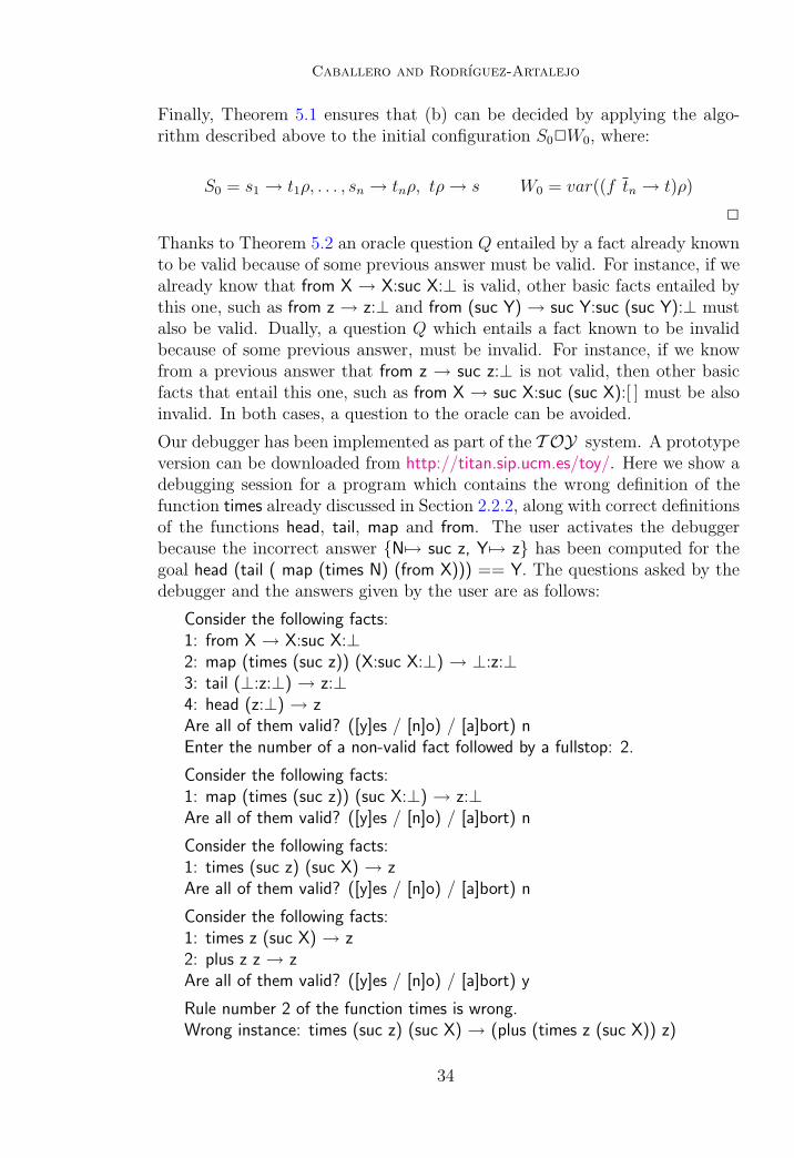
Caballero and Rodrıguez-Artalejo
Finally, Theorem 5.1 ensures that (b) can be decided by applying the algo-rithm described above to the initial configuration S02W0, where:
S0 = s1 → t1ρ, . . . , sn → tnρ, tρ→ s W0 = var((f tn → t)ρ)
2
Thanks to Theorem 5.2 an oracle question Q entailed by a fact already knownto be valid because of some previous answer must be valid. For instance, if wealready know that from X → X:suc X:⊥ is valid, other basic facts entailed bythis one, such as from z → z:⊥ and from (suc Y) → suc Y:suc (suc Y):⊥ mustalso be valid. Dually, a question Q which entails a fact known to be invalidbecause of some previous answer, must be invalid. For instance, if we knowfrom a previous answer that from z → suc z:⊥ is not valid, then other basicfacts that entail this one, such as from X → suc X:suc (suc X):[ ] must be alsoinvalid. In both cases, a question to the oracle can be avoided.
Our debugger has been implemented as part of the T OY system. A prototypeversion can be downloaded from http://titan.sip.ucm.es/toy/. Here we show adebugging session for a program which contains the wrong definition of thefunction times already discussed in Section 2.2.2, along with correct definitionsof the functions head, tail, map and from. The user activates the debuggerbecause the incorrect answer {N 7→ suc z, Y7→ z} has been computed for thegoal head (tail ( map (times N) (from X))) == Y. The questions asked by thedebugger and the answers given by the user are as follows:
Consider the following facts:1: from X → X:suc X:⊥2: map (times (suc z)) (X:suc X:⊥) → ⊥:z:⊥3: tail (⊥:z:⊥) → z:⊥4: head (z:⊥) → zAre all of them valid? ([y]es / [n]o) / [a]bort) nEnter the number of a non-valid fact followed by a fullstop: 2.
Consider the following facts:1: map (times (suc z)) (suc X:⊥) → z:⊥Are all of them valid? ([y]es / [n]o) / [a]bort) n
Consider the following facts:1: times (suc z) (suc X) → zAre all of them valid? ([y]es / [n]o) / [a]bort) n
Consider the following facts:1: times z (suc X) → z2: plus z z → zAre all of them valid? ([y]es / [n]o) / [a]bort) y
Rule number 2 of the function times is wrong.Wrong instance: times (suc z) (suc X) → (plus (times z (suc X)) z)
34
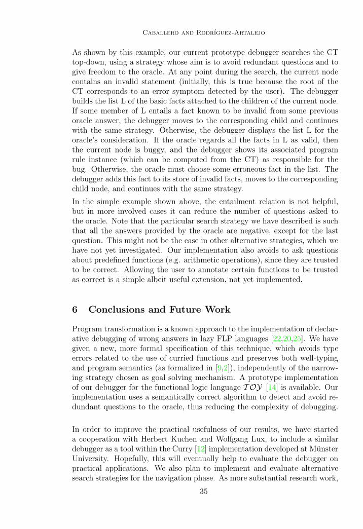
Caballero and Rodrıguez-Artalejo
As shown by this example, our current prototype debugger searches the CTtop-down, using a strategy whose aim is to avoid redundant questions and togive freedom to the oracle. At any point during the search, the current nodecontains an invalid statement (initially, this is true because the root of theCT corresponds to an error symptom detected by the user). The debuggerbuilds the list L of the basic facts attached to the children of the current node.If some member of L entails a fact known to be invalid from some previousoracle answer, the debugger moves to the corresponding child and continueswith the same strategy. Otherwise, the debugger displays the list L for theoracle’s consideration. If the oracle regards all the facts in L as valid, thenthe current node is buggy, and the debugger shows its associated programrule instance (which can be computed from the CT) as responsible for thebug. Otherwise, the oracle must choose some erroneous fact in the list. Thedebugger adds this fact to its store of invalid facts, moves to the correspondingchild node, and continues with the same strategy.
In the simple example shown above, the entailment relation is not helpful,but in more involved cases it can reduce the number of questions asked tothe oracle. Note that the particular search strategy we have described is suchthat all the answers provided by the oracle are negative, except for the lastquestion. This might not be the case in other alternative strategies, which wehave not yet investigated. Our implementation also avoids to ask questionsabout predefined functions (e.g. arithmetic operations), since they are trustedto be correct. Allowing the user to annotate certain functions to be trustedas correct is a simple albeit useful extension, not yet implemented.
6 Conclusions and Future Work
Program transformation is a known approach to the implementation of declar-ative debugging of wrong answers in lazy FLP languages [22,20,25]. We havegiven a new, more formal specification of this technique, which avoids typeerrors related to the use of curried functions and preserves both well-typingand program semantics (as formalized in [9,2]), independently of the narrow-ing strategy chosen as goal solving mechanism. A prototype implementationof our debugger for the functional logic language T OY [14] is available. Ourimplementation uses a semantically correct algorithm to detect and avoid re-dundant questions to the oracle, thus reducing the complexity of debugging.
In order to improve the practical usefulness of our results, we have starteda cooperation with Herbert Kuchen and Wolfgang Lux, to include a similardebugger as a tool within the Curry [12] implementation developed at MunsterUniversity. Hopefully, this will eventually help to evaluate the debugger onpractical applications. We also plan to implement and evaluate alternativesearch strategies for the navigation phase. As more substantial research work,
35
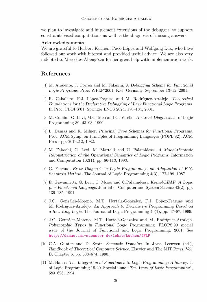
Caballero and Rodrıguez-Artalejo
we plan to investigate and implement extensions of the debugger, to supportconstraint-based computations as well as the diagnosis of missing answers.
AcknowledgementsWe are grateful to Herbert Kuchen, Paco Lopez and Wolfgang Lux, who havefollowed our work with interest and provided useful advice. We are also veryindebted to Mercedes Abengozar for her great help with implementation work.
References
[1] M. Alpuente, J. Correa and M. Falaschi. A Debugging Scheme for FunctionalLogic Programs. Proc. WFLP’2001, Kiel, Germany, September 13–15, 2001.
[2] R. Caballero, F.J. Lopez-Fraguas and M. Rodrıguez-Artalejo. TheoreticalFoundations for the Declarative Debugging of Lazy Functional Logic Programs.In Proc. FLOPS’01, Springer LNCS 2024, 170–184, 2001.
[3] M. Comini, G. Levi, M.C. Meo and G. Vitello. Abstract Diagnosis. J. of LogicProgramming 39, 43–93, 1999.
[4] L. Damas and R. Milner. Principal Type Schemes for Functional Programs.Proc. ACM Symp. on Principles of Programming Languages (POPL’82), ACMPress, pp. 207–212, 1982.
[5] M. Falaschi, G. Levi, M. Martelli and C. Palamidessi. A Model-theoreticReconstruction of the Operational Semantics of Logic Programs. Informationand Computation 102(1). pp. 86-113, 1993.
[6] G. Ferrand. Error Diagnosis in Logic Programming, an Adaptation of E.Y.Shapiro’s Method. The Journal of Logic Programming 4(3), 177-198, 1987.
[7] E. Giovannetti, G. Levi, C. Moiso and C.Palamidessi. Kernel-LEAF: A Logicplus Functional Language. Journal of Computer and System Science 42(2), pp.139–185, 1991.
[8] J.C. Gonzalez-Moreno, M.T. Hortala-Gonzalez, F.J. Lopez-Fraguas andM. Rodrıguez-Artalejo. An Approach to Declarative Programming Based ona Rewriting Logic. The Journal of Logic Programming 40(1), pp. 47–87, 1999.
[9] J.C. Gonzalez-Moreno, M.T. Hortala-Gonzalez and M. Rodrıguez-Artalejo.Polymorphic Types in Functional Logic Programming. FLOPS’99 specialissue of the Journal of Functional and Logic Programming, 2001. Seehttp://danae.uni-muenster.de/lehre/kuchen/JFLP
[10] C.A. Gunter and D. Scott. Semantic Domains. In J.van Leeuwen (ed.),Handbook of Theoretical Computer Science, Elsevier and The MIT Press, Vol.B, Chapter 6, pp. 633–674, 1990.
[11] M. Hanus. The Integration of Functions into Logic Programming: A Survey. J.of Logic Programming 19-20. Special issue “Ten Years of Logic Programming”,583–628, 1994.
36
Caballero and Rodrıguez-Artalejo
[12] M. Hanus (ed.). Curry: An Integrated Functional Logic Language. Version 0.7,February 2, 2000.Available at http://www.informatik.uni-kiel.de/curry/.
[13] J.W. Lloyd. Declarative Error Diagnosis. New Generation Computing 5(2), 133–154, 1987.
[14] F.J. Lopez-Fraguas, J. Sanchez-Hernandez. T OY: A Multiparadigm DeclarativeSystem. In Proc. RTA’99, Springer LNCS 1631, pp 244–247, 1999. Available athttp://titan.sip.ucm.es/toy.
[15] R. Milner. A Theory of Type Polymorphism in Programming. Journal ofComputer and Systems Sciences, 17, pp. 348–375, 1978.
[16] B. Moller. On the Algebraic Specification of Infinite Objects - Ordered andContinuous Models of Algebraic Types. Acta Informatica 22, pp. 537–578, 1985.
[17] L. Naish. Declarative Diagnossing of Missing Answers. New GenerationComputing, 10, 255–385, 1991.
[18] L. Naish. Declarative Debugging of Lazy Functional Programs. AustralianComputer Science Communications, 15(1):287–294, 1993.
[19] L. Naish. A Declarative Debugging Scheme. Journal of Functional and LogicProgramming, 1997-3.
[20] L. Naish and T. Barbour. Towards a Portable Lazy Functional DeclarativeDebugger. Australian Computer Science Communications, 18(1):401–408, 1996.
[21] H. Nilsson, P. Fritzson. Algorithmic Debugging of Lazy Funcional Languages.The Journal of Functional Programming, 4(3):337-370, 1994.
[22] H. Nilsson and J. Sparud. The Evaluation Dependence Tree as a basis for LazyFunctional Debugging. Automated Software Engineering, 4(2):121–150, 1997.
[23] H. Nilsson. Declarative Debugging for Lazy Functional Languages. Ph.D.Thesis. Dissertation No. 530. Univ. Linkoping, Sweden. 1998.
[24] S.L. Peyton Jones (ed.), J. Hughes (ed.), L. Augustsson, D. Barton, B. Boutel,W. Burton, J. Fasel, K. Hammond, R. Hinze, P. Hudak, T. Johnsson,M.P. Jones, J. Launchbury, E. Meijer, J. Peterson, A. Reid, C. Runciman andP. Wadler. Report on the programming language Haskell 98: a non-strict, purelyfunctional language. Available at http://www.haskell.org/definition,February 1999.
[25] B. Pope. Buddha. A Declarative Debugger for Haskell. Honours Thesis,Department of Computer Science, University of Melbourne, Australia, June1998.
[26] E.Y. Shapiro. Algorithmic Program Debugging. The MIT Press, Cambridge,Mass., 1982.
37
Caballero and Rodrıguez-Artalejo
[27] J. Sparud. Tracing and Debuggging Lazy Functional Computations. PhDThesis. Department of Computer Science, Chalmers Universitity of Technology.Goteborg, Sweden, 1999.
[28] A. Tessier and G. Ferrand. Declarative Diagnosis in the CLP Scheme. InP. Deransart, M. Hermenegildo and J. Ma luszynski (Eds.), Analysis andVisualization Tools for Constraint Programming, Chapter 5, pp. 151–174.Springer LNCS 1870, 2000.
[29] P. Wadler. Why no one uses Functional Languages. SIGPLAN Notices 33(8),23–27, 1998.
38
Caballero and Rodrıguez-Artalejo
7 Appendix A: Proofs of the main results
7.1 Proofs of Results from Section 2
Proof of Theorem 2.2This theorem is also based on some auxiliary lemmata.
Lemma 7.1 For any given Herbrand interpretation I, the analogous of Propo-sition 2.1 holds for the calculus SCI, i.e.:
(i) For all t, s ∈ Pat⊥: t→ s is valid in I iff t w s.
(ii) For all e ∈ Exp⊥, t, s ∈ Pat⊥: if e → t is valid in I and t w s, thene→ s is also valid in I.
(iii) For all e ∈ Exp⊥, t ∈ Pat⊥ and θ, θ′ ∈ Subst⊥ such that eθ → t is validin I and θ v θ′, the statement eθ′ → t is also valid in I, with a SCIproof of the same size and structure.
(iv) For all e ∈ Exp⊥, s ∈ Pat⊥ such that e→ s is valid in I, the statementeθ → sθ is also valid in I for every total substitution θ ∈ Subst.
Proof Idea. This can be proved by straightforward induction on the size ofSCI derivations, similarly to Proposition 2.1. 2
Lemma 7.2 Assume a Herbrand interpretation I, a partial expression e ∈Exp⊥ and a partial pattern t ∈ Pat⊥. Then [[e]]I ⊇ [[t]]I iff t ∈ [[e]]I.
Proof. Assume [[e]]I ⊇ [[t]]I . By Lemma 7.1, t → t is valid in I. Thent ∈ [[t]]I and therefore t ∈ [[e]]I . Conversely, suppose that t ∈ [[e]]I . Then e→ tis valid in I, and for all s ∈ [[t]]I , t → s is also valid in I. By Lemma 7.1 itfollows that e→ s is valid in I for all s ∈ [[t]]I , which means [[e]]I ⊇ [[t]]I . 2
Lemma 7.3 Let I a Herbrand interpretation and f tn → s a basic fact. Thenf tn → s is valid in I iff (f tn → s) ∈ I.
Proof. If s =⊥ the result holds because f tn →⊥ belongs to every Herbrandinterpretation and f tn →⊥ is valid in I due to the SCI rule BT . In the restof the proof we assume that s is not ⊥.
If (f tn → s) ∈ I then f tn → s is valid in I, as witnessed by the followingSCI derivation, ending with a FAI step:
t1 → t1 . . . tn → tn s→ s (f tn → s) ∈ I
f tn → s
The derivation can be completed because Lemma 7.1 ensures that all thepremises ti → ti and s→ s are valid in I.
Conversely, if f tn → s is valid in I, there is a SCI proof of f tn → s, which
39
Caballero and Rodrıguez-Artalejo
must end with a FAI step and have the following form:
t1 → t′1 . . . tn → t′n s′ → s (f t′n → s′) ∈ I
f tn → s
By Lemma 7.1 we can conclude that t′1 v t1, . . . , t′n v tn and s v s′. Since
(f t′n → s′) ∈ I, item (ii) from the definition of Herbrand interpretation inSection 2.3.4 implies (f tn → s) ∈ I. 2
Lemma 7.4 Let P any program and MP = {f tn → s | P `SC f tn → s}.Then MP is a Herbrand interpretation.
Proof. MP must satisfy the three conditions of Herbrand interpretations:
(i) (f tn →⊥) ∈MP .This property holds since f tn →⊥ can be proved in SC by means of theBT rule.
(ii) If (f tn → s) ∈MP , ti v t′i, s w s′ then (f t′n → s′) ∈MP .This follows immediately from the definition ofMP and Proposition 2.1.
(iii) If (f tn → s) ∈MP and θ ∈ Subst is a total substitution, then(f tn → s)θ ∈MP . This is also a straigthforward consequence of Propo-sition 2.1 and the construction of MP .
2
We are now ready to prove claims (a), (c) and (b) of Theorem 2.2, in thisorder.
(a) Let ϕ be a statement such that P `SC ϕ and assume that I is a Herbrandmodel of P . Let T be the proof tree of ϕ in SC. We will build a proof treeT ′ of ϕ in SCI , showing that ϕ is valid in I. This is done by using inductionon the depth of T .
Basis: (depth(T)= 0). Then ϕ is the only node of T and corresponds eitherto a BT , DC or to a RR inference. Since these rules are also present in SCIwe can take T ′ = T .
Inductive step: (depth(T)= n, n > 0). We distinguish different cases depend-ing on the SC rule applied at the root of T .
DC: In this case ϕ must have the form h em → h tm and the inference stepat the root of T must be:
e1 → t1 . . . em → tm
h em → h tm
Since ruleDC also exists in SCI we can build T ′ with the same root as T andwith the same children at the root. Moreover by the induction hypothesisthe ei → ti are valid in I and therefore there exist proof trees in SCI that
40
Caballero and Rodrıguez-Artalejo
will complete the construction of T ′.
JN: In this case ϕ has the form e == e′ and the inference step at the rootof T must be:
e→ t e′ → t
e == e′
where t is a total pattern. Since rule JN also exists in SCI we can build T ′
with the same root as T and with the same children at the root. Moroverby the induction hypothesis the e → t, e′ → t are valid in I and thereforethere exist proof trees in SCI that will complete the construction of T ′.
AR + FA: In this case ϕ has the form f en am → t and the SC inferenceat the root of T must be:
C r → s
e1 → t1 . . . en → tn f tn → s s am → t
f en am → t
Then we build T ′ by using rule FAI at the root:
e1 → t1 . . . en → tn s am → t (f tn → s) ∈ I
f en am → t
and completing the proof tree by means of SCI proof trees for the state-ments ei → ti and s am → t, which exist by induction hypothesis, sinceall these statements have proof trees of depth less than n in SC. However,we still have to check that the conditions required by FAI are satisfied.First t is actually a pattern different from ⊥ because this condition is alsorequired by rule AR + FA. To see that f tn → s is in I we observe thatf t1 . . . tn → t ⇐ C is an instance of some rewrite rule belonging to P .Moreover, I satisfies C by induction hypothesis. Since I is a model of P ,we can conclude that [[f t1 . . . tn]]I ⊇ [[r]]I . By induction hypothesis we alsoknow that r → s is valid in I. It follows that s ∈ [[r]]I ⊆ [[ft1 . . . tn]]I andhence s ∈ [[ft1 . . . tn]]I , as we needed.
(c) MP is an Herbrand interpretation as shown in Lemma 7.4. Assume thatϕ is valid inMP with proof tree T in SCMP
. Then we show by induction ondepth(T ) that we can build a proof tree T ′ for ϕ in SC.
Basis (depth(T ) = 0). The only possible inferences applied at the root of Tare BT , RR or DC. Since these 3 rules belong also to SC we can take T ′ = T .
Inductive Step (depth(T ) = n, n > 0). Then either DC, JN or FAMPhas
been applied at the root of T . In the DC and JN cases, the same inference
41
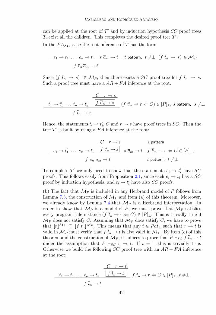
Caballero and Rodrıguez-Artalejo
can be applied at the root of T ′ and by induction hypothesis SC proof treesTi exist all the children. This completes the desired proof tree T ′.
In the FAMPcase the root inference of T has the form
e1 → t1 . . . en → tn s am → t t pattern, t 6=⊥, (f tn → s) ∈MP
f en am → t
Since (f tn → s) ∈ MP , then there exists a SC proof tree for f tn → s.Such a proof tree must have a AR + FA inference at the root:
C r → s
t1 → t′1 . . . tn → t′nf t′n → s (f t′n → r ⇐ C) ∈ [P ]⊥, s pattern, s 6=⊥
f tn → s
Hence, the statements ti → t′i, C and r → s have proof trees in SC. Then thetree T ′ is built by using a FA inference at the root:
C r → s s pattern
e1 → t′1 . . . en → t′nf t′n → s s am → t f t′n → r ⇐ C ∈ [P ]⊥,
f en am → t t pattern, t 6=⊥
To complete T ′ we only need to show that the statements ei → t′i have SCproofs. This follows easily from Proposition 2.1, since each ei → ti has a SCproof by induction hypothesis, and ti → t′i have also SC proofs.
(b) The fact that MP is included in any Herbrand model of P follows fromLemma 7.3, the construction ofMP and item (a) of this theorem. Moreover,we already know by Lemma 7.4 that MP is a Herbrand interpretation. Inorder to show that MP is a model of P , we must prove that MP satisfiesevery program rule instance (f tn → r ⇐ C) ∈ [P ]⊥. This is trivially true ifMP does not satisfy C. Assuming thatMP does satisfy C, we have to provethat [[r]]MP ⊆ [[f tn]]MP . This means that any t ∈ Pat⊥ such that r → t isvalid inMP must verify that f tn → t is also valid inMP . By item (c) of thistheorem and the construction ofMP , it suffices to prove that P `SC f tn → tunder the assumption that P `SC r → t. If t = ⊥ this is trivially true.Otherwise we build the following SC proof tree with an AR + FA inferenceat the root:
C r → t
t1 → t1 . . . tn → tn f tn → t f tn → r ⇐ C ∈ [P ]⊥, t 6=⊥
f tn → t
42
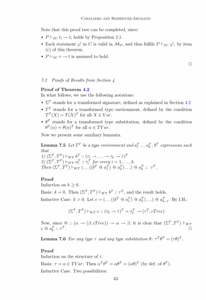
Caballero and Rodrıguez-Artalejo
Note that this proof tree can be completed, since:
• P `SC ti → ti holds by Proposition 2.1.
• Each statement ϕ′ in C is valid in MP , and thus fulfils P `SC ϕ′, by item(c) of this theorem.
• P `SC r → t is assumed to hold.
2
7.2 Proofs of Results from Section 4
Proof of Theorem 4.2In what follows, we use the following notations:
• ΣT stands for a transformed signature, defined as explained in Section 4.2
• T T stands for a transformed type environment, defined by the conditionT T (X) = T (X)T for all X ∈ V ar.
• θT stands for a transformed type substitution, defined by the conditionθT (α) = θ(α)T for all α ∈ TV ar.
Now we present some auxiliary lemmata.
Lemma 7.5 Let T T be a type environment and aT1 . . . aTk , bT expressions such
that1) (ΣT , T T ) `WT b
T :: (τ1 → . . .→ τk → τ)T
2) (ΣT , T T ) `WT aTi :: τTi for every i = 1, . . . , k.
Then (ΣT , T T ) `WT (. . . ((bT @ aT1 ) @ aT2 ) . . .) @ aTk :: τT .
ProofInduction on k ≥ 0.
Basis: k = 0. Then (ΣT , T T ) `WT bT :: τT , and the result holds.
Inductive Case: k > 0. Let e = (. . . ((bT @ aT1 ) @ aT2 ) . . .) @ aTk−1. By I.H.:
(ΣT , T T ) `WT e :: (τk → τ)T = τTk → (τT , cT ree)
Now, since @ :: (α → (β, cTree)) → α → β, it is clear that (ΣT , T T ) `WT
e @ aTk :: τT . 2
Lemma 7.6 For any type τ and any type substitution θ: τT θT = (τθ)T .
ProofInduction on the structure of τ .
Basis: τ = α ∈ TV ar. Then αT θT = αθT = (αθ)T (by def. of θT ).
Inductive Case. Two possibilities:
43
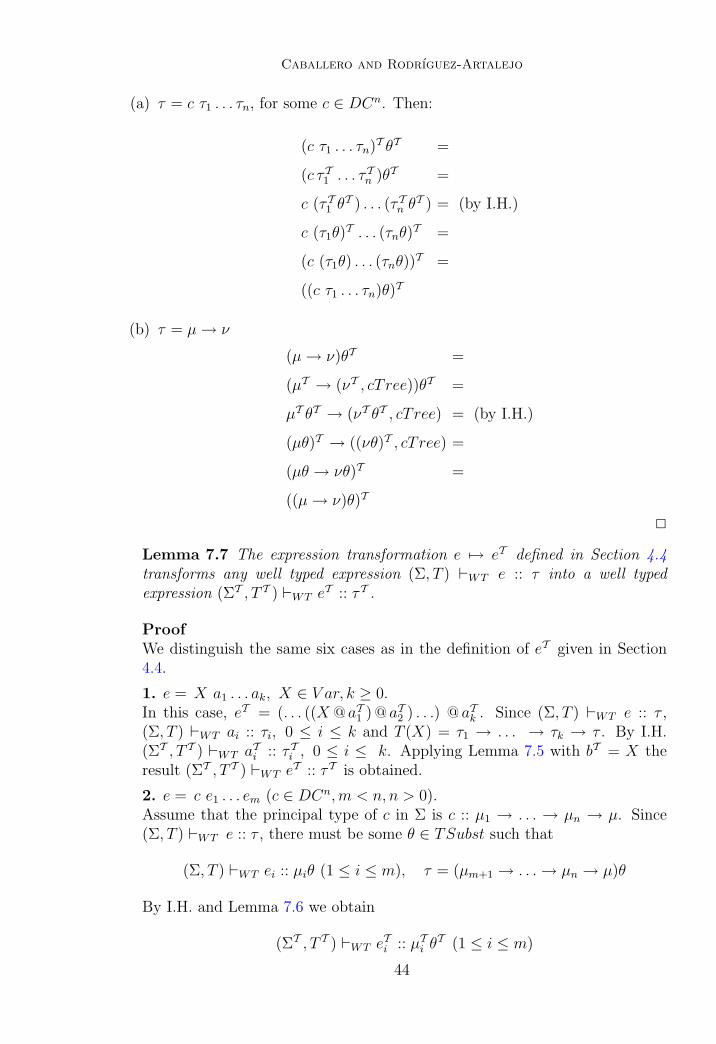
Caballero and Rodrıguez-Artalejo
(a) τ = c τ1 . . . τn, for some c ∈ DCn. Then:
(c τ1 . . . τn)T θT =
(c τT1 . . . τTn )θT =
c (τT1 θT ) . . . (τTn θ
T ) = (by I.H.)
c (τ1θ)T . . . (τnθ)
T =
(c (τ1θ) . . . (τnθ))T =
((c τ1 . . . τn)θ)T
(b) τ = µ→ ν
(µ→ ν)θT =
(µT → (νT , cT ree))θT =
µT θT → (νT θT , cT ree) = (by I.H.)
(µθ)T → ((νθ)T , cT ree) =
(µθ → νθ)T =
((µ→ ν)θ)T
2
Lemma 7.7 The expression transformation e 7→ eT defined in Section 4.4transforms any well typed expression (Σ, T ) `WT e :: τ into a well typedexpression (ΣT , T T ) `WT e
T :: τT .
ProofWe distinguish the same six cases as in the definition of eT given in Section4.4.
1. e = X a1 . . . ak, X ∈ V ar, k ≥ 0.In this case, eT = (. . . ((X @ aT1 ) @ aT2 ) . . .) @ aTk . Since (Σ, T ) `WT e :: τ ,(Σ, T ) `WT ai :: τi, 0 ≤ i ≤ k and T (X) = τ1 → . . . → τk → τ . By I.H.(ΣT , T T ) `WT a
Ti :: τTi , 0 ≤ i ≤ k. Applying Lemma 7.5 with bT = X the
result (ΣT , T T ) `WT eT :: τT is obtained.
2. e = c e1 . . . em (c ∈ DCn,m < n, n > 0).Assume that the principal type of c in Σ is c :: µ1 → . . . → µn → µ. Since(Σ, T ) `WT e :: τ , there must be some θ ∈ TSubst such that
(Σ, T ) `WT ei :: µiθ (1 ≤ i ≤ m), τ = (µm+1 → . . .→ µn → µ)θ
By I.H. and Lemma 7.6 we obtain
(ΣT , T T ) `WT eTi :: µTi θ
T (1 ≤ i ≤ m)
44
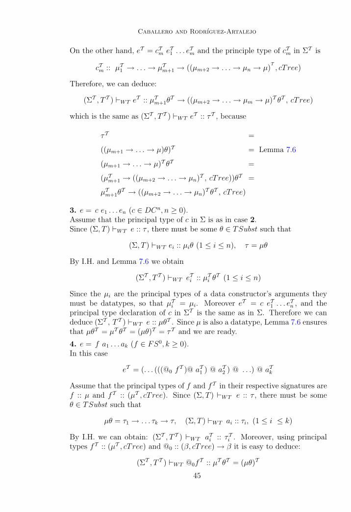
Caballero and Rodrıguez-Artalejo
On the other hand, eT = cTm eT1 . . . eTm and the principle type of cTm in ΣT is
cTm :: µT1 → . . .→ µTm+1 → ((µm+2 → . . .→ µn → µ)T, cT ree)
Therefore, we can deduce:
(ΣT , T T ) `WT eT :: µTm+1θ
T → ((µm+2 → . . .→ µm → µ)T θT , cT ree)
which is the same as (ΣT , T T ) `WT eT :: τT , because
τT =
((µm+1 → . . .→ µ)θ)T = Lemma 7.6
(µm+1 → . . .→ µ)T θT =
(µTm+1 → ((µm+2 → . . .→ µn)T , cT ree))θT =
µTm+1θT → ((µm+2 → . . .→ µn)T θT , cT ree)
3. e = c e1 . . . en (c ∈ DCn, n ≥ 0).Assume that the principal type of c in Σ is as in case 2.Since (Σ, T ) `WT e :: τ , there must be some θ ∈ TSubst such that
(Σ, T ) `WT ei :: µiθ (1 ≤ i ≤ n), τ = µθ
By I.H. and Lemma 7.6 we obtain
(ΣT , T T ) `WT eTi :: µTi θT (1 ≤ i ≤ n)
Since the µi are the principal types of a data constructor’s arguments theymust be datatypes, so that µTi = µi. Moreover eT = c eT1 . . . e
Tn , and the
principal type declaration of c in ΣT is the same as in Σ. Therefore we candeduce (ΣT , T T ) `WT e :: µθT . Since µ is also a datatype, Lemma 7.6 ensuresthat µθT = µT θT = (µθ)T = τT and we are ready.
4. e = f a1 . . . ak (f ∈ FS0, k ≥ 0).In this case
eT = (. . . (((@0 fT )@ aT1 ) @ aT2 ) @ . . .) @ aTk
Assume that the principal types of f and fT in their respective signatures aref :: µ and fT :: (µT , cT ree). Since (Σ, T ) `WT e :: τ , there must be someθ ∈ TSubst such that
µθ = τ1 → . . . τk → τ, (Σ, T ) `WT ai :: τi, (1 ≤ i ≤ k)
By I.H. we can obtain: (ΣT , T T ) `WT aTi :: τTi . Moreover, using principaltypes fT :: (µT , cT ree) and @0 :: (β, cTree)→ β it is easy to deduce:
(ΣT , T T ) `WT @0fT :: µT θT = (µθ)T
45
Caballero and Rodrıguez-Artalejo
where the last equality holds by Lemma 7.6. Now:
(µθ)T = (τ1 → . . .→ τk → τ)T
and Lemma 7.5 can be applied (with b = f) to obtain
(Σ, T ) `WT (. . . (((@0 fT )@ aT1 ) @ aT2 ) @ . . .) @ aTk :: τT
which is the same as (Σ, T ) `WT eT :: τT .
5. e = f e1 . . . em (f ∈ FSn, n > 0,m < n− 1).Analogous to case 2.
6. e = f e1 . . . en−1 a1 . . . ak (f ∈ FSn, n > 0, k ≥ 0).In this case
eT = (. . . ((fT eT1 . . . eTn−1) @ aT1 ) @ aT2 ) @ . . .) @ aTk
The principal types of f and fT in their respective signatures must be of theform
f :: µ1 → . . .→ µn → µ, fT :: µT1 → . . .→ µTn → (µT , cT ree)
Since (Σ, T ) `WT e :: τ , there must be some θ ∈ TSubst such that
(µ1 → . . .→ µn → µ)θ = τ1 → . . .→ τn−1 → ν1 → . . .→ νk → τ
with
(Σ, T ) `WT ei :: τi (1 ≤ i ≤ n− 1), (Σ, T ) `WT aj :: νj (1 ≤ j ≤ k)
By I.H. we obtain:
(ΣT , T T ) `WT eTi :: τTi (1 ≤ i ≤ n− 1), (ΣT , T T ) `WT a
Tj :: νTj (1 ≤ j ≤ k)
Using the principal type of fT in ΣT as well as Lemma 7.6 we can deduce:
(ΣT , T T ) `WT fT eT1 . . . eTn−1 :: µTn θ
T → (µT θT , cT ree) = Lemma 7.6
µnθT → (µθT , cT ree) =
((µn → µ)θ)T =
(ν1 → . . .→ νk → ν)T
Now we can apply Lemma 7.5 to obtain
(ΣT , T T ) `WT (. . . ((fT eT1 . . . eTn−1) @ aT1 ) @ aT2 ) @ . . .) @ aTk :: τT
which is the same as (ΣT , T T ) `WT eT :: τT . 2
46
Caballero and Rodrıguez-Artalejo
Lemma 7.8 Any simple application of the transformation rules AP0 or AP1
defined in Section 4.4 preservers well-typing. More precisely: if a partiallytransformed program rule is well-typed w.r.t. a type environment T Ti , then thenew program rule obtained by one single application of AP0 or AP1 is alsowell-typed w.r.t. some type environment T Ti+1 with type assumptions for somenew variables.
Proof.
Both transformation rules AP0, AP1 transform only the part of the rule corre-sponding to the local declarations, and hence we only need to check that thispart is well-typed.
• Rule AP0 transforms{. . . ; p← e[@0 fun]; . . . T ← cNode . . . (clean lp)} into{. . . ; (R′, T ′)← fun; p← e[R′]; . . . T ← cNode . . . (clean (lp++[(dVal R′, T ′)]))}There must exist a type environment T Ti such that:
(1) (ΣT , T Ti ) `WT p :: τ :: e[@0 fun], with τ ′ the type used for (@0 fun) inthe proof.(2) (ΣT , T Ti ) `WT T :: cTree :: (cNode . . . (clean (lp ++[(dVal R′, T ′)]))),with [(pV al, cTree)] the type used for lp in the proof.
Then we define T Ti+1 by extending T Ti with suitable types for the new variablesR′ and T ′:
T Ti+1 = T Ti ⊕ {R′ :: τ ′, T ′ :: cTree}Since τ ′ is the type of (@0 fun) in (1), then:
(ΣT , T Ti ) `WT @0 :: (τ ′, cT ree)→ τ ′, (ΣT , T Ti ) `WT fun :: (τ ′, cT ree)
Then obviously
(ΣT , Ti+1) `WT (R′, T ′) :: (τ ′, cT ree) :: fun, (ΣT , Ti+1) `WT p :: τ :: e[R′]
Finally, since dV al :: A → pV al, (++) :: [A] → [A] → [A] ∈ ΣT , and usingthe types for T, lp in (2)
(ΣT , Ti+1) `WT (lp++[(dVal R′, T ′)])) :: [(pV al, cTree)]
and hence:
(ΣT , Ti+1) `WT (cNode . . . (clean (lp++[(dVal R′, T ′)]))) :: cTree
as expected.
• Rule AP1: The proof is very similar to the case of rule AP0.
2
47
Caballero and Rodrıguez-Artalejo
Now we are ready to prove Theorem 4.2:
In P T there are new functions such as clean, dVal, functions for partial appli-cations and constructors, as well as functions coming from the transformationof functions in P (see Section 4.4. We must prove that all these of functionsare well-typed.
• Function dVal is a primitive and therefore we only can assume that it is well-typed. Checking that clean is well-typed is straightforward from its definition.
• Auxiliary functions fT0 , . . . , fTn−2 for f ∈ FSn. Two cases:
(1) fTm , m < n− 2The only rule for
fTm :: τT1 → . . .→ τTm+1 → ((τm+2 → . . .→ τn → τ)T, cT ree)
is fTm Xm+1 → (fTm+1 Xm+1, void). We define a new type environment:
T T = {X1 :: τT1 , . . . , Xm+1 :: τTm+1}
which ensures:a) (ΣT , T T ) `WT Xm+1 :: τT m+1.b) (ΣT , T T ) `WT f
Tm+1 Xm+1 :: τTm+2 → ((τm+3 → . . .→ τn → τ)
T, cT ree) =
((τm+2 → τm+3 → . . .→ τn → τ)T, cT ree).
c) (ΣT , T T ) `WT void :: cTree
(2) fTn−2
The only rule for fTn−2 :: τT1 → . . .→ τTn−1 → ((τn → τ)T, cT ree) is
fTn−2 Xn−1 → (fT Xn−1, void), and by defining the same type environment
T as above and since fT :: τT1 → . . . → τTn → (τT, cT ree), the result can
be checked as in the previous case.
• Auxiliary functions cT0 , . . . , cTn−1 for c ∈ DCn. Analogous to the previous
case.
• Transformed functions.The well-typedness of transformed functions can be checked in two steps:
1) Assuming a well-type program rule in P :
(R) f t1 . . . tn → r ⇐ . . . li == ri . . . where{. . . sj ← dj; . . .}
For a function with principal type declaration f : τ1 → τn → τ , the trans-formed function has principal type fT : τT1 → . . . → τTn → (τT , cT ree) andthe transformed program rule looks initially as follows, before starting to applythe transformations AP0 and AP1 to the local definitions:
48
Caballero and Rodrıguez-Artalejo
(RT0 ) fT tT1 . . . tTn → (R, T )⇐ . . . CLi == CRi . . .
where{ . . .
sTj ← dTj ;. . .
CLi ← lTi ;CRi ← rTi ;
. . .
R ← rT ;T ← cNode ”f” [dV al tT1 , . . . dV al t
Tn ] (dV al R) ”f.j” (clean [ ])}
In order to prove that the previous partially transformed program rule is well-typed, we consider a type environment T which well-types the original programrule in the sense defined in Section 2.2.1. We define T T0 in the following way:
T T0 (X) = (T (X))T for all X ∈ dom(T ).T T0 (R) = τT with τ s.t. (Σ, T ) `WT r :: τ .T T0 (T ) = cTree.T T0 (CLi) = T T0 (CRi) = νTi with νi s.t. (Σ, T ) `WT li :: νi :: ri.
Now:- Since (R) well-typed, (Σ, T ) `WT ti :: τi. By Lemma 7.7,
(ΣT , T T ) `WT tTi :: τTi
- (ΣT , T T ) `WT (R, T ) :: (τT , cT ree).
- (ΣT , T T ) `WT CLi :: νTi :: CRi.
- Since (R) well-typed, (Σ, T ) `WT sj :: υ :: dj. By Lemma 7.7,
(ΣT , T T ) `WT sTj :: υT :: dTj
- Also, by Lemma 7.7, and the construction of T T :
(ΣT , T T ) `WT CLi :: νTi :: lTi
(ΣT , T T ) `WT CRi :: νTi :: rTi
(ΣT , T T ) `WT R :: τT :: rT
- Finally is easy to check from the signature of cNode, dV al and clean that:
(ΣT , T T ) `WT
(cNode ”f” [dV al tT1 , . . . , dV al tTn ] (dV al R) ”f.j” (clean [ ])) :: cTree
49
Caballero and Rodrıguez-Artalejo
and. by definition
(ΣT , T T ) `WT T : cTree
Therefore the initial transformation is well-typed.
2) The consecutive application of rules AP0 and AP1 transform a well-typedrule into a new well-typed rule. This follows from Lemma 7.8.Since each rule AP0 and AP1 reduces the number either the number of either@0 or @, and the number of these symbols is finite, the process will end in awell-typed rule.
2
Proof of Theorem 4.3
The proof of this theorem depends on the specification of the semantic calculusFSCT used for deductions with transformed programs. This is presentedbelow:
Definition 7.9 The calculus FSCT consists of the rules of FSC (i.e. rulesBT , RR, DC, JN and FA of the SC described in Section 2.3.1) plus twonew rule schemes dV al and SFA (meaning Suspended Function Application)defined as follows:
• (dV al) dval tT → dte
where:- t can be any pattern in the original signature.- tT is the transformation of pattern t as described in Section 4.2.- dte is the representation of t as string.
• (SFA) callT → (⊥,⊥)
Here callT can be any partial expression which has one of the forms gT sT m(with g ∈ FSm, m ≥ 0) or (F sT )ρT (F variable, s pattern, ρ ∈ Subst⊥).
Before starting the proof we observe that the SC deduction P `SC f tn → tcan be replaced by PF `FSC f tn → t due to the semantic correctness offlattening (Theorem 4.1). Now we are ready to prove items (i) and (ii) of thetheorem.
(i) Assume a FSC proof tree T witnessing PF `FSC f tn → t with associatedAPT apt. Reasoning by induction on the structure of T we show that it ispossible to find a total ct :: cTree representing apt such that
P T `FSCT fT tT n → (tT , ct)
Since t 6=⊥, the inference step at the root of T must be a FA step using one ofthe defining rules for f in PF instantiated by some ρ ∈ Subst⊥. Let us consider
50
Caballero and Rodrıguez-Artalejo
this program rule rlF ∈ PF along with the corresponding program rules rl ∈ Pand rlT ∈ P T respectively. In the sequel we assume that rlT and rlF have theforms shown at the end of Section 4.4 and in Section 4.7, respectively, exceptthat the left-hand sides are now assumed to be fT pT1 . . . pTn and f p1 . . . pn,respectively. In the reasonings below, we make implicit use of Proposition 2.1and Lemma 7.6 at several places.
The substitution ρ must be such that the inference step at the root of T aswell as the rest of T succeed. Therefore we can assume:(1) pnρ = tn.
(2) PF `FSC Rρ→ t i.e. t v Rρ (since t, Rρ patterns).
(3) PF `FSC (callk → Rk)ρ for each condition Rk ← callk in rlF (proved bysubtrees Tk of T with smaller size than T ).
(4)PF `FSC (sj ← wj)ρ i.e. sjρ v wjρ for each condition sj ← wj in rlF(since sjρ, wjρ are patterns).
(5) PF `FSC (LSi ← ui)ρ and PF `FSC (RSi ← vi)ρ i.e. LSiρ v uiρand RSiρ v viρ (since LSiρ, uiρ, RSiρ, viρ are patterns) for all conditionsLSi ← ui, RSi ← vi in rlF .
(6) PF `FSC (R← v)ρ i.e. Rρ v vρ, since Rρ, vρ are patterns.
Now we look for a corresponding ρT ∈ SubstT⊥ defined in such a way that wecan build a FSCT proof tree T ′ witnessing P T `FSCT fT tTn → (tT , ct),so that the inference step at the root of T ′ will be a FA inference using theρT -instance of the program rule rlT . As a partial definition of ρT we assume:ρT (X) = ρ(X)T for all X ∈ dom(ρ). The effect of ρT over those variables ofrlT which do not appear in rlF (namely T and the various Tk) will be definedlater. Presently, the partial definition of ρT allows us to draw some conclu-sions from items (1)− (6) above:
(1′) pTn ρT = (pnρ)T = tT n.
(2′) tT v RρT i.e. P T `FSCT RρT → tT (since tT , RρT patterns).
(3′) Each condition (Rk, Tk)← callTk in rlT corresponds to Rk ← callk in rlF .Here we can distinguish three cases:
(3.1′) Rkρ 6=⊥ and callk = g sm for some g ∈ FSm, m ≥ 0 and somepatterns sm. Then callTk ρ
T = gT sTmρT = gT (smρ)T and by I.H. applied to
PF `FSC g smρ→ Rkρ we can assume P T `FSCT callTk ρT → (Rkρ
T , ctk)where ctk :: cTree represents aptk, the APT extracted from Tk.
((3.2′) Rkρ 6=⊥ and callk = F s with F variable. Since Fρ and sρ arepatterns, PF `FSC (F s → Rk)ρ, and Rkρ 6=⊥, it follows that Fρ mustbe a rigid pattern. We consider different subcases according to the form ofFρ:
51
Caballero and Rodrıguez-Artalejo
(3.2.1′) Fρ = c sm, m ≥ 0, ar(c) = m+ 1, c ∈ DC.Since PF `FSC Fρ sρ→ Rkρ, sρ must be a pattern s.t. Rkρ v c sm sρ.Moreover:callTk ρ
T = (F sT )ρT = ((c sm)T ) (sT ρT ) = (cT m sT m) (sT ρT ). The laststep holds because of the definition of the transformation T . P T includesthe program rule cT m Xm+1 → (c Xm+1, void). Using this rule andRkρ
T v c sT m (sT ρT ), we can derive:
P T `FSCT cTm sT m (sT ρT )→ (RkρT , void)
i.e.
P T `FSCT callTk ρT → (RkρT , void)
(3.2.2′) Fρ = c sm, m ≥ 0 ar(c) > m + 1, c ∈ DC. Analogous to theprevious case but using the P T rule cTm Xm+1 → (cTm+1, void).
(3.2.3′) Fρ = g sm, m ≥ 0 ar(g) = m+ 1, g ∈ FS. In this case:
callTk ρT = (F sT )ρT = (g sm)T (sT ρT ) = gT sT m (sT ρT )
By I.H. applied to PF `FSC g sm (sρ) → Rkρ we arrive to the sameconclusion as in case (3.1′), namely: P T `FSCT callTk → (Rkρ
T , ctk)where ctk :: cTree represents the APT extracted from Tk.
(3.2.4′) Fρ = g sm, m ≥ 0, ar(g) > m + 1, g ∈ FS. Similarly to (3.2.1′),since PF `FSC (Fρ) (sρ) → Rkρ, sρ must be s.t. Rkρ v g sm (sρ).Moreover callTk ρT = (F sT )ρT = (g sm)T (sT ρT ) = gTm sT m (sT ρT ), andP T includes one of the two following defining rules:(R1) gTm Xm+1 → (gT Xm+1, void) if m+ 2 < ar(g).(R2) gTm Xm+1 → (gT Xm+1, void) if m+ 2 = ar(g).In the case m+ 2 < arg(g) we have:• P T `FSCT callTk ρT → (gTm+1 s
Tm (sT ρT ), void) using (R1).
• RkρT v ((g sm)(sρ))T = gTm+1 s
Tm (sT ρT ).
Similarly, in the case m+ 2 = arg(g):
• P T `FSCT callTk ρT → (gT sTm (sT ρT ), void) using (R2).• Rkρ
T v ((g sm)(sρ))T = gT sT m (sT ρT ).
In both cases, we can conclude that P T `FSCT callTk ρT → (Rkρ
T , void).
(3.3′) Rkρ =⊥. In this case Tk must reduce to one single step, applying theSC inference BT, and we can establish no definite conclusion about callkρ,except that it must have one of the following forms:(∗) g sm, with g ∈ FSm, m ≥ 0; sm patterns.(∗∗) (F s)ρ, which might be even flexible if Fρ = F .In both cases, we can use the special FSCT -inference SFA to derive:P T `FSCT callTk → (⊥,⊥).
52
Caballero and Rodrıguez-Artalejo
(4′) (sjρ)T v (wjρ)T i.e. sTj ρT v wTj ρ
T i.e. P T `FSCT (sTj ← wTj )ρT foreach condition sTj ← wTj in rlT (since sTj ρ
T , wTj ρT are patterns).
(5′) (LSiρ)T v (uiρ)T i.e. LSiρT v uTi ρ
T i.e. P T `FSCT (LSi ← uTi )ρT and(RSiρ)T v (viρ)T i.e. RSiρ
T v vTi ρT i.e. P T `FSCT (RSi ← vTi )ρT ,
for each condition LSi ← uTi , RSi ← vTi in rlT , (LSiρT , uTi ρ
T , RSTi ρT , vTi ρ
T
are patterns).
(6′) (Rρ)T v (vρ)T i.e. RρT v vT ρT i.e. P T `FSCT (R← vT )ρ, (RρT , vT ρT
are patterns).
At this point we can complete the definition of ρT by requiring:• ρT (Tk) = ctk, for all those k corresponding to case (3.1′) or case (3.2.3′).• ρ(Tk) = void, for all those k corresponding to some of the cases (3.2.1′),(3.2.2′), (3.2.4′).• ρT (Tk) =⊥, for all those k corresponding to case (3.3′).• ρ(T ) = cNode ”f” [dtT1
e, . . . , dtTne] dRρT e ”f.ind” [. . . ctk . . . ]
where:- dtTi
e (1 ≤ i ≤ n), dRρT e are the representations of the patterns tTi (1 ≤ i ≤ n),RρT as strings.- ”f” resp. ”f.ind” are the strings which represent the symbol f and the symbolf followed by the index member of the program rule rl (among the programrules for f , taken in textual order).- [. . . ctk . . . ] is the list of all those ctk corresponding to cases (3.1′), (3.2.3′).
Let ct = ρT (T ). We claim that P T `FSCT fT tT n → (tT , ct) and thatct :: cTree represents apt, the APT extracted from the FSC proof tree Twhich proved PF `FSC f tn → t. To justify the claim we build a FSCT
proof tree T ′ whose last step is a FA inference using the ρT -instance of theprogram rule rlT ∈ P T . Items (1′)− (6′) show that the instantiated rule canbe applied, and that all the conditions occurring as premises of FA, exceptthe last one, can be proved by means of FSCT derivations. The last conditionis:
(T ← cNode ” f”[dV al pT1 , . . . , dV al pTn ] (dV al R)
”f.ind” (clean[. . . (dV al Rk, Tk) . . .]))ρT
This can be also derived from P T in FSCT , because:• TρT is ct, as defined above.• For all i ≤ i ≤ n, dV al (pTi ρ
T ) = dV al tTi , and P T `FSCT dV al tTi →dtTie by the special FSCT -inference (dV al).
• P T `FSCT dV al RρT → dRρT e also because of (dV al).• P T `FSCT clean [. . . , (dV al Rk, Tk)ρ
T , . . .]→ [. . . , ctk, . . .],where [. . . , ctk, . . .] stands for the list of those ctk corresponding to cases(3.1′), (3.2.3′). This follows from the definition of clean, because those kwhich correspond to other cases are such that either Rkρ
T =⊥ (and thenP T `FSCT dV al Rkρ
T → d ⊥ e, P T `FSCT isBottom d ⊥ e → true) or
53
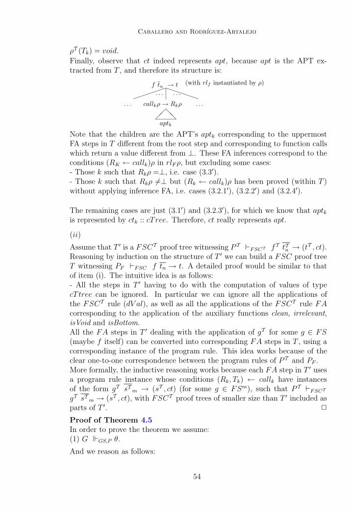
Caballero and Rodrıguez-Artalejo
ρT (Tk) = void.
Finally, observe that ct indeed represents apt, because apt is the APT ex-tracted from T , and therefore its structure is:
f tn → t (with rlf instantiated by ρ)�����
. . . callkρ→ Rkρ . . .
. . . . . .PPPPP
��@@
aptk
Note that the children are the APT’s aptk corresponding to the uppermostFA steps in T different from the root step and corresponding to function callswhich return a value different from ⊥. These FA inferences correspond to theconditions (RK ← callk)ρ in rlFρ, but excluding some cases:- Those k such that Rkρ =⊥, i.e. case (3.3′).- Those k such that Rkρ 6=⊥ but (Rk ← callk)ρ has been proved (within T )without applying inference FA, i.e. cases (3.2.1′), (3.2.2′) and (3.2.4′).
The remaining cases are just (3.1′) and (3.2.3′), for which we know that aptkis represented by ctk :: cTree. Therefore, ct really represents apt.
(ii)
Assume that T ′ is a FSCT proof tree witnessing P T `FSCT fT tTn → (tT , ct).Reasoning by induction on the structure of T ′ we can build a FSC proof treeT witnessing PF `FSC f tn → t. A detailed proof would be similar to thatof item (i). The intuitive idea is as follows:- All the steps in T ′ having to do with the computation of values of typecT tree can be ignored. In particular we can ignore all the applications ofthe FSCT rule (dV al), as well as all the applications of the FSCT rule FAcorresponding to the application of the auxiliary functions clean, irrelevant,isVoid and isBottom.All the FA steps in T ′ dealing with the application of gT for some g ∈ FS(maybe f itself) can be converted into corresponding FA steps in T , using acorresponding instance of the program rule. This idea works because of theclear one-to-one correspondence between the program rules of P T and PF .More formally, the inductive reasoning works because each FA step in T ′ usesa program rule instance whose conditions (Rk, Tk) ← callk have instancesof the form gT sT m → (sT , ct) (for some g ∈ FSm), such that P T `FSCTgT sT m → (sT , ct), with FSCT proof trees of smaller size than T ′ included asparts of T ′. 2
Proof of Theorem 4.5In order to prove the theorem we assume:(1) G GS,P θ.
And we reason as follows:
54
Caballero and Rodrıguez-Artalejo
(2) sol Xnθ == true 1stGS,Psol id , by (1) and stability of GS.
(3) Psol `SC sol Xnθ → true with APT apt which can be extracted from thecomputation (2). By (2) and soundness of GS.
(4) P Tsol `FSCT solT XnθT → (true, ct) where ct :: cTree represents apt.
This holds by (3) and the semantic correctness of the program transformation(Theorem 4.3, item (i)).
(5) solT XnθT == (true, T ) 1st
GS,PTsol{T 7→ ct}. By (2), (3), (4) and weak
completeness of GS.
Note that ct represents apt, an APT witnessing (3). Due to the definition ofsol in Psol, apt serves also as witness of P `SC Gθ. 2
7.3 Proofs of Results from Section 5
Proof of Theorem 5.1First we present two auxiliary lemmata.
Lemma 7.10 Let Si2Wi be a configuration obtained after i steps of the al-gorithm described in Section 5, and (s→ t) ∈ Si.Then var(s) ∩Wi = ∅ ∨ var(t) ∩Wi = ∅.
Proof
We reason by induction on i.Basis. The result holds for the first configuration because of the constructionof S0 and W0, since the two initial basic facts have no common variables.
Inductive step.Consider the i-th step of the algorithm (i ≥ 1): Si−12Wi−1 `θi Si2Wi. Lets→ t be any approximation statement in Si. We can distinguish two cases:
- s → t = (a → b)θi for some a → b in Si−1. By I.H. either a or b (or both)share no variables with Wi−1. Assume that var(a) ∩Wi−1 = ∅ (analogous forb). Then, since dom(θi) ⊆Wi−1, s = aθi = a and since Wi coincides with Wi−1
except for the possible addition of some new fresh variables, var(s)∩Wi = ∅.- s→ t is some of the new approximation statements introduced either by ruleR3 or R6. In the case of R3, each ai → bi must fulfill the result, applying I.H.to h am → h bm. The case of R6 it is clear from I.H. that var(h am)∩Wi−1 = ∅and therefore also var(ai) ∩Wi = ∅ for all 1 ≥ i ≥ m. 2
Lemma 7.11 Let Si2Wi `θi+1Si+12Wi+1 be some step of the algorithm de-
scribed in Sect. 5. Then Sol(Si2Wi) = (θi+1Sol(Si+12Wi+1))�Wi.
ProofThe Lemma can be proved by examining the transformation rule applied atthe given step. In the case of rules R1, R2 and R3, θi+1 = id, Wi+1 = Wi
and the result follows from the definition of the approximation ordering v, as
55
Caballero and Rodrıguez-Artalejo
given in Section 2.1. Rules R4, R5 and R6 are considered below.
R4 Sol(s→ X,S2W ) = {X 7→ s}Sol(S{X 7→ s}2W )a) Sol(s→ X,S2W ) ⊆ {X 7→ s}Sol(S{X 7→ s}2W )Let θ ∈ Sol(s→ X,S2W ). Then:- Xθ = sθ, since Xθ v sθ and θ is a total substitution.- Sθ holds- θ = {X 7→ s}θ, because for any Y ∈ V ar, if Y 6= X then Y {X 7→ s}θ = Y θand if Y = X then Y {X 7→ s}θ = sθ = Xθ = Y θ.Therefore S{X 7→ s}θ = Sθ holds, and hence θ ∈ Sol(S{X 7→ s}2W ).Finally, considering again that θ = {X 7→ s}θ, the expected resultθ ∈ {X 7→ s}Sol(S{X 7→ s}2W ) is obtained.
b) {X 7→ s}Sol(S{X 7→ s}2W ) ⊆ Sol(s→ X,S2W )Any element in {X 7→ s}Sol(S{X 7→ s}2W ) must be of the form {X 7→ s}θ,with θ ∈ Sol(S{X 7→ s}2W ). Then:- S{X 7→ s}θ holds.- s{X 7→ s}θ = X{X 7→ s}θ. To check this, note that X /∈ var(s), becauseX ∈ W implies var(s) ∩W = ∅, by Lemma 7.10. Then s{X 7→ s}θ = sθ =X{X 7→ s}θ.Hence {X 7→ s}θ ∈ Sol(s→ X,S2W ).
R5 Sol(X → Y, S2W ) = {X 7→ Y }Sol(S{X 7→ Y }2W )Analogous to the previous case.
R6 Sol(X → h am, S2W ) =({X 7→ hXm}Sol(. . . , Xk → ak, . . . , S{X 7→ hXm}2W,Xm)�W
a) Sol(X → h am, S2W ) ⊆({X 7→ hXm}Sol(. . . , Xk → ak, . . . , S{X 7→ hXm}2W,Xm)�W
Let θ ∈ Sol(X → h am, S2W ). Then:- Xθ = h tm with akθ v tk.- Sθ holds.Consider the total substitution ρ =def θ ∪· {X1 7→ t1, . . . , Xm 7→ tm}. Then :- Xkρ = tk, akρ = akθ and therefore akρ v Xkρ.- S{X 7→ hXm}ρ = Sθ holds.Hence ρ ∈ Sol(. . . , Xk → ak, . . . , S{X 7→ hXm}2W,Xm).Moreover {X 7→ hXm}ρ�W = θ.Therefore θ ∈ ({X 7→ hXm}Sol(. . . , Xk → ak, . . . , S{X 7→ hXm}2W,Xm)�W .
b) ({X 7→ hXm}Sol(. . . , Xk → ak, . . . , S{X 7→ hXm}2W,Xm)�W ⊆Sol(X → h am, S2W )
Any member of ({X 7→ hXm}Sol(. . . , Xk → ak, . . . , S{X 7→ hXm}2W,Xm)�Wmust be of the form θ = ({X 7→ hXm}ρ)�W withρ ∈ Sol(. . . , Xk → ak, . . . , S{X 7→ hXm}2W,Xm) s.t.:
56
Caballero and Rodrıguez-Artalejo
(1) For each k, akρ v Xkρ holds.(2) S{X 7→ hXm}ρ = holds.By Lemma 7.10, and since X ∈W , var(ak) ∩W = ∅.Also, var(ak) ∩ (W,Xm) = ∅, since Xm are fresh variables.Therefore akρ v Xkρ iff ak v Xkρ. Calling bk to each Xkρ:(3) akρ v Xkρ iff ak v bk.
This means that θ must be of the form θ = {X 7→ h bm} ∪· ρ�(W−{X}).Then:- (X → h am)θ = h bm → h am which holds iff for each k ak v bk which is trueby (3) and (1).- Sθ = S({X 7→ h bm}∪· ρ�(W−{X})) = S{X 7→ hXm}ρ which holds by (2). 2
Now, Theorem 5.1 can be proved as follows:
To prove that the algorithm is terminating we define a well founded lexico-graphic order between configurations.We say that Ki < Kj (with Ki = Si2Wi, Kj = Sj2Wj) iffa) ||Ki ||1 < ||Kj ||1, orb) ||Ki ||1 = ||Kj ||1 and ||Ki ||2 < ||Kj ||2, orc) ||Ki ||1 = ||Kj ||1 and ||Ki ||2 = ||Kj ||2, and ||Ki ||3 < ||Kj ||3.where:
• ||S2W ||1 = number of occurrences of rigid patterns h am, m ≥ 0 in some(s→ t) ∈ S s.t.:
a) If h am is part of s then var(t) ∩W 6= ∅.b) If h am is part of t then var(s) ∩W 6= ∅.
• ||S2W ||2 = number of occurrences of symbols h ∈ DC ∪ FS in S.
• ||S2W ||3 = size of S (as a multiset, counting repetitions).
Now it suffices to check that at each step of the algorithm Ki+1 < Ki. Thiscan be done by examining the transformation rule applied at this step, as wellas the selected (s→ t) ∈ Si:
R1 Then ||Ki+1 ||1 = ||Ki ||1, ||Ki+1 ||2 = ||Ki ||2, and ||Ki+1 ||3 < ||Ki ||3.
R2 Then ||Ki+1 ||1 = ||Ki ||1, and either- ||Ki+1 ||2 = ||Ki ||2, ||Ki+1 ||3 < ||Ki ||3 (if t ∈ V ar)or- ||Ki+1 ||2 < ||Ki ||2 (if t is not a variable).
R3 Either ||Ki+1 ||1 < ||Ki ||1, or ||Ki+1 ||1 = ||Ki ||1 and ||Ki+1 ||2 < ||Ki ||2
57
Caballero and Rodrıguez-Artalejo
(since symbol h is removed in Si+1).
R4 The algorithm step is, in this case, of the form:
s→ X, S2W︸ ︷︷ ︸
Ki
`{X 7→s} S{X 7→ s}2W︸ ︷︷ ︸
Ki+1
, X 6= s,X ∈W
If s is a variable then ||Ki+1 ||1 = ||Ki ||1, ||Ki+1 ||2 = ||Ki ||2, and||Ki+1 ||3 < ||Ki ||3. If s is not a variable then it is a rigid pattern. Then,since X ∈W , Lemma 7.10 ensures that
||S{X 7→ s}2W ||1 = ||S2W ||1 < || s→ X, S2W ||1
i.e. ||Ki+1 ||1 < ||Ki ||1.
R5 Then ||Ki+1 ||1 = ||Ki ||1, ||Ki+1 ||2 = ||Ki ||2, and ||Ki+1 ||3 < ||Ki ||3.
R6 Analogously to R4 when s is not a variable: ||Ki+1 ||1 < ||Ki ||1.Next we prove that if Sj 6= ∅ then Sol(S02W0) = ∅ and hence there is nosubstitution θ that solves the system and the entailment does not hold. ByLemma 7.11 it is enough to show that Sol(Sj2Wj) = ∅. Since no rule trans-formation can be applied to this configuration, at least one of the cases belowmust hold. Notice that in every case the system cannot be solved.a) ⊥→ s ∈ Sj, s 6=⊥. Then there exists no total substitution θ such thatsθ v⊥.b) h am → g bl with either h 6= g or m 6= l. Obvious.c) h am → X, h am not total, X ∈ Wj. Then there is no total substitution θs.t. Xθ ⊆ (h am)θ.d) X → Y , X 6= Y , X /∈Wj, Y /∈Wj. Straightforward, from the requirementof dom(θ) ⊆Wj in every solution.e) X → h am, X /∈Wj. As the previous case.
Finally, if Sj = ∅ thenSol(∅2Wj) = SubstWj
where SubstWj= {θ ∈ Subst | dom(θ) ⊆Wj}.
We consider the substitution θ = θ1θ2 . . . θj.By Lemma 7.11, Sol(S02W0) = (θSubstWj
)�W0 .Since id ∈ SubstWj
, θid �W0= θ �W0∈ Sol(S02W0), and hence θ �W0 can beused to prove the entailment between both basic facts. 2
58
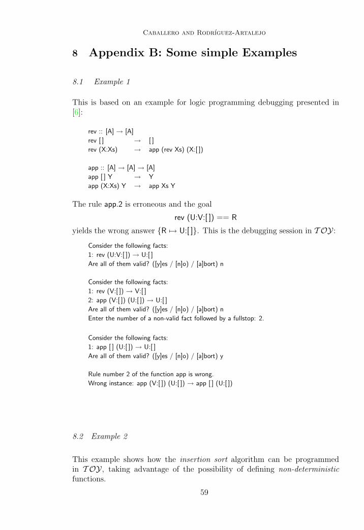
Caballero and Rodrıguez-Artalejo
8 Appendix B: Some simple Examples
8.1 Example 1
This is based on an example for logic programming debugging presented in[6]:
rev :: [A] → [A]
rev [ ] → [ ]
rev (X:Xs) → app (rev Xs) (X:[ ])
app :: [A] → [A] → [A]
app [ ] Y → Y
app (X:Xs) Y → app Xs Y
The rule app.2 is erroneous and the goal
rev (U:V:[ ]) == R
yields the wrong answer {R 7→ U:[ ]}. This is the debugging session in T OY:
Consider the following facts:
1: rev (U:V:[ ]) → U:[ ]
Are all of them valid? ([y]es / [n]o) / [a]bort) n
Consider the following facts:
1: rev (V:[ ]) → V:[ ]
2: app (V:[ ]) (U:[ ]) → U:[ ]
Are all of them valid? ([y]es / [n]o) / [a]bort) n
Enter the number of a non-valid fact followed by a fullstop: 2.
Consider the following facts:
1: app [ ] (U:[ ]) → U:[ ]
Are all of them valid? ([y]es / [n]o) / [a]bort) y
Rule number 2 of the function app is wrong.
Wrong instance: app (V:[ ]) (U:[ ]) → app [ ] (U:[ ])
8.2 Example 2
This example shows how the insertion sort algorithm can be programmedin T OY, taking advantage of the possibility of defining non-deterministicfunctions.
59
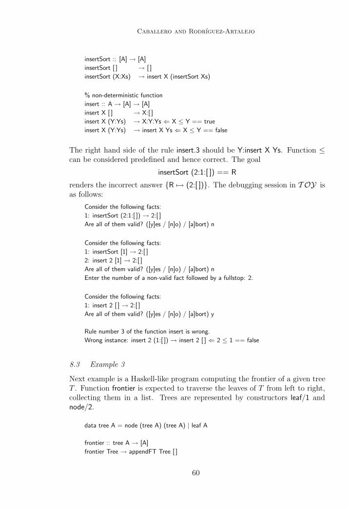
Caballero and Rodrıguez-Artalejo
insertSort :: [A] → [A]
insertSort [ ] → [ ]
insertSort (X:Xs) → insert X (insertSort Xs)
% non-deterministic function
insert :: A → [A] → [A]
insert X [ ] → X:[ ]
insert X (Y:Ys) → X:Y:Ys ⇐ X ≤ Y == true
insert X (Y:Ys) → insert X Ys ⇐ X ≤ Y == false
The right hand side of the rule insert.3 should be Y:insert X Ys. Function ≤can be considered predefined and hence correct. The goal
insertSort (2:1:[ ]) == R
renders the incorrect answer {R 7→ (2:[ ])}. The debugging session in T OY isas follows:
Consider the following facts:
1: insertSort (2:1:[ ]) → 2:[ ]
Are all of them valid? ([y]es / [n]o) / [a]bort) n
Consider the following facts:
1: insertSort [1] → 2:[ ]
2: insert 2 [1] → 2:[ ]
Are all of them valid? ([y]es / [n]o) / [a]bort) n
Enter the number of a non-valid fact followed by a fullstop: 2.
Consider the following facts:
1: insert 2 [ ] → 2:[ ]
Are all of them valid? ([y]es / [n]o) / [a]bort) y
Rule number 3 of the function insert is wrong.
Wrong instance: insert 2 (1:[ ]) → insert 2 [ ] ⇐ 2 ≤ 1 == false
8.3 Example 3
Next example is a Haskell-like program computing the frontier of a given treeT . Function frontier is expected to traverse the leaves of T from left to right,collecting them in a list. Trees are represented by constructors leaf/1 andnode/2.
data tree A = node (tree A) (tree A) | leaf A
frontier :: tree A → [A]
frontier Tree → appendFT Tree [ ]
60
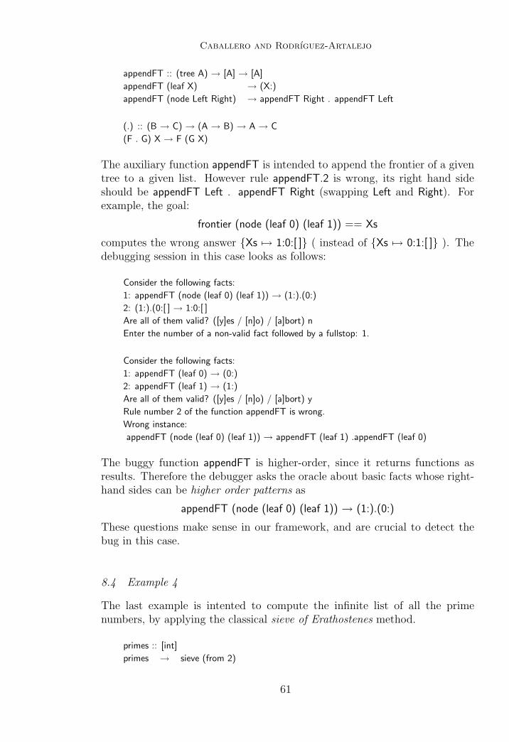
Caballero and Rodrıguez-Artalejo
appendFT :: (tree A) → [A] → [A]
appendFT (leaf X) → (X:)
appendFT (node Left Right) → appendFT Right . appendFT Left
(.) :: (B → C) → (A → B) → A → C
(F . G) X → F (G X)
The auxiliary function appendFT is intended to append the frontier of a giventree to a given list. However rule appendFT.2 is wrong, its right hand sideshould be appendFT Left . appendFT Right (swapping Left and Right). Forexample, the goal:
frontier (node (leaf 0) (leaf 1)) == Xs
computes the wrong answer {Xs 7→ 1:0:[ ]} ( instead of {Xs 7→ 0:1:[ ]} ). Thedebugging session in this case looks as follows:
Consider the following facts:
1: appendFT (node (leaf 0) (leaf 1)) → (1:).(0:)
2: (1:).(0:[ ] → 1:0:[ ]
Are all of them valid? ([y]es / [n]o) / [a]bort) n
Enter the number of a non-valid fact followed by a fullstop: 1.
Consider the following facts:
1: appendFT (leaf 0) → (0:)
2: appendFT (leaf 1) → (1:)
Are all of them valid? ([y]es / [n]o) / [a]bort) y
Rule number 2 of the function appendFT is wrong.
Wrong instance:
appendFT (node (leaf 0) (leaf 1)) → appendFT (leaf 1) .appendFT (leaf 0)
The buggy function appendFT is higher-order, since it returns functions asresults. Therefore the debugger asks the oracle about basic facts whose right-hand sides can be higher order patterns as
appendFT (node (leaf 0) (leaf 1)) → (1:).(0:)
These questions make sense in our framework, and are crucial to detect thebug in this case.
8.4 Example 4
The last example is intented to compute the infinite list of all the primenumbers, by applying the classical sieve of Erathostenes method.
primes :: [int]
primes → sieve (from 2)
61
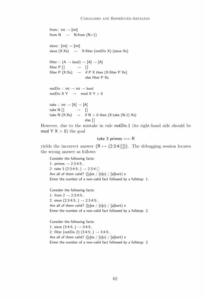
Caballero and Rodrıguez-Artalejo
from:: int → [int]
from N → N:from (N+1)
sieve:: [int] → [int]
sieve (X:Xs) → X:filter (notDiv X) (sieve Xs)
filter :: (A → bool) → [A] → [A]
filter P [ ] → [ ]
filter P (X:Xs) → if P X then (X:filter P Xs)
else filter P Xs
notDiv :: int → int → bool
notDiv X Y → mod X Y > 0
take :: int → [A] → [A]
take N [ ] → [ ]
take N (X:Xs) → if N > 0 then (X:take (N-1) Xs)
else [ ]
However, due to the mistake in rule notDiv.1 (its right-hand side should bemod Y X > 0) the goal
take 3 primes == R
yields the incorrect answer {R 7→ (2:3:4:[ ])}. The debugging session locatesthe wrong answer as follows:
Consider the following facts:
1: primes → 2:3:4:5:
2: take 3 (2:3:4:5: ) → 2:3:4:[ ]Are all of them valid? ([y]es / [n]o) / [a]bort) n
Enter the number of a non-valid fact followed by a fullstop: 1.
Consider the following facts:
1: from 2 → 2:3:4:5:
2: sieve (2:3:4:5: ) → 2:3:4:5:
Are all of them valid? ([y]es / [n]o) / [a]bort) n
Enter the number of a non-valid fact followed by a fullstop: 2.
Consider the following facts:
1: sieve (3:4:5: ) → 3:4:5:
2: filter (notDiv 2) (3:4:5: ) → 3:4:5:
Are all of them valid? ([y]es / [n]o) / [a]bort) n
Enter the number of a non-valid fact followed by a fullstop: 2.
62

Caballero and Rodrıguez-Artalejo
Consider the following facts:
1: notDiv 2 3 → true
2: filter (notDiv 2) (4:5: ) → 4:5:
Are all of them valid? ([y]es / [n]o) / [a]bort) n
Enter the number of a non-valid fact followed by a fullstop: 2.
Consider the following facts:
1: notDiv 2 4 → true
2: filter (notDiv 2) (5: ) → 5:
Are all of them valid? ([y]es / [n]o) / [a]bort) n
Enter the number of a non-valid fact followed by a fullstop: 1.
Rule number 1 of the function notDiv is wrong.
Wrong instance: notDiv 2 4 → (mod 2 4) > 0
Notice the occurrence of symbol (representing ⊥) in many basic facts of thesession, approximating results of subcomputations that were not needed.
63