Data Centric Highly Parallel Debugging

§ David Abramson, Minh Ngoc Dinh, Donny Kurniawan † Bob Moench, Luiz DeRose

§ Faculty of Information Technology,

Monash University, Clayton, 3800, Victoria, Australia

† Cray Inc,

Cray Plaza, 380 Jackson St, Suite 210 St. Paul, MN 55101 USA

Abstract

Debugging parallel programs is an order of magnitude more complex than sequential ones, and yet, most parallel debuggers provide little extra functionality than their sequential counterparts. This problem becomes more serious as computational codes become more complex, involving larger data structures, and as the machines become larger. Peta-scale machines consisting of millions of cores pose a significant challenge for existing techniques. We argue that debugging must become more data-centric, and believe that “assertions” provide a useful model. Assertions allow a user to declare their expectations about the program state as a whole rather than focusing on that of only a single process state. Previously, we have implemented a special type of assertion that supports debugging applications as they evolve or are ported to different platforms. They allow a user to compare the state of one program against another reference version. These ‘relative debugging’ assertions, whilst powerful, pose significant implementation challenges for large peta-scale machines. In this paper we discuss a hashing technique that provides a scalable solution for very large problems on very large machines. We illustrate the scheme on 65k cores of Kraken, a Cray XT5 at the University of Tennessee. Categories and Subject Descriptors !"#"$%&'()*++,(-%.+'/+0112(/3%

!"4"5%6,7-2(/%0(8%!,9*//2(/%

!"#$%&'().0+0::,:%&'1;*-2(/<%!,9*//2(/"%

1 Introduction Traditionally, sequential program debuggers allow a user to control the execution of a program to examine and alter the state of variables. There have been relatively few advances in parallel debugging technology over the years, and adoption by users is still

relatively low. Interestingly, most parallel debuggers use the same paradigm as their sequential counterparts, and either allow a user to focus on a single process of interest, or aggregate a set of processes to present a unified view. Thus, debuggers such as TotalView [1], DDT [2], LadeBug [3], Mantis [4], and Eclipse (PTP) [5] allow users to display the state of processes in a predefined process set using various reduction techniques. This makes it possible to observe overall patterns in the data and spot outliers.

Whilst these ideas are powerful, the growth in both the size of the structures manipulated by modern scientific codes, and the number of cores, make existing techniques unwieldy. A number of researchers have discussed the need for a more data-centric view of debugging than the traditional control flow techniques [6-8]. In a data-centric view, a user makes statements about the contents of data structures, and the veracity of these are checked by the debugger.

Assertion constructs have been available in programming languages for some time, and these allow a programmer to make statements about the state of a program that are checked at run time [9-11]. Assertions have been used extensively for evaluating invariants [10], checking input parameters [9], and for enhancing program correctness and quality. To a limited extent, assertions have also been incorporated into some sequential debuggers [6-8, 12, 13]. Assertions support a more data centric view of debugging because the user does not focus on the control path per se, but can assert that various data structures should be in particular states at various stages in the program execution. The following examples illustrate the potential for such assertions in debugging a program: • The contents of this array should always be

positive; • The sum of the contents of this array should always

be less than a constant bound; • The value in this scalar should always be greater

than the value of another scalar variable; and

Permission to make digital or hard copies of all or part of this work for personal or classroom use is granted without fee provided that copies are not made or distributed for profit or commercial advantage and that copies bear this notice and the full citation on the first page. To copy otherwise, to republish, to post on servers or to redistribute to lists, requires prior specificpermission and/or a fee.HPDC'10, June 20–25, 2010, Chicago, Illinois, USA.Copyright 2010 ACM 978-1-60558-942-8/10/06 ...$10.00.

119

• The contents of this array should always be the same as the contents in another array. Evaluating assertions in a very large parallel

machine poses a number of implementation as well as performance issues. First, the debugger requires an understanding of the way the data is decomposed across the parallel processors. This is because the assertion may pertain to a data structure that is distributed and may never exist in a single node. Second, as a consequence of the first point, the assertion must be evaluated in each of the processors, requiring a debugging architecture that understands how data has been decomposed and distributed across the processors. Importantly, if the assertion evaluation is executed in parallel, then the technique scales as the machine size increases.

We are interested in a type of assertion, used in a technique called relative debugging [13], that allows a user to compare the state of two different programs. Relative debugging allows a user to find errors that are introduced when a program is ported to a new machine, or modified to incorporate parallel computing techniques, because one version of the code is used for establishing reference values for assertions.

Implementing relative debugging assertions poses additional implementation difficulties over general assertions. For example, a naive implementation of relative debugging extracts data from two programs and compares it sequentially in a single (head) node of the cluster. This approach fails to scale to large problems on large machines because there is insufficient room to store all of the data. Further, and more dramatic, the transmission of data from each of the nodes, and the sequential comparison would take too long for large machines.

In this paper we discuss a hashing technique that executes relative debugging assertion in two phases. First, every processor hashes the data structure to produce a small set of signatures. Second, the array of signatures is recursively combined and compared in the head node. The scheme is highly scalable because hashing operations can be performed in parallel; and the amount of data to transfer and compare is relatively small. However, many challenges must be addressed if the technique is to be feasible. The paper starts with an overview of relative debugging, followed by a detailed design of the hashing technique we proposed. We evaluate the performance of our approach using a kernel implementation, written in MPI and implemented on 65,536 cores of a 99,072 core Cray XT5. Importantly, many of the ideas presented here for executing relative debugging assertions are applicable to other forms of data-centric assertions.

2 Relative Debugging and Guard 2.1 Overview Relative debugging helps a programmer locate errors in programs by observing the divergence in key data structures as the programs are executing [13-15]. In particular, it allows comparison of a suspect program against a reference code using assertions. It is a particularly valuable technique when a program is ported to, or rewritten for, another computer platform. Relative debugging is effective because the user can concentrate on where two related codes are producing different results, rather than being concerned with the actual values in the data structures. Various case studies reporting the results of using relative debugging have been published [16-18], and these have demonstrated the efficiency of the technique. The concept of relative debugging is both language and machine independent. It allows a user to compare data structures without concern for the implementation, and thus attention can be focused on the cause of the errors rather than implementation details.

A relative debugger uses a declarative assertion, which consists of a combination of data structure names, process identifiers and breakpoint locations. Assertions are processed by the debugger before program execution commences, and an internal graph is built which describes when the two programs must pause, and which data structures are to be compared. In the following example:

assert $reference::BigVar@4300 = $suspect::LargeVar@4400 the debugger compares data from BigVar in $reference at line 4300 with LargeVar in $suspect at line 4400. User can formulate as many assertions as necessary, and can refine them after the programs have begun execution. This makes it possible to locate an error by placing new assertions iteratively until the region is small enough to inspect manually. This process is very efficient. Even if the programs are millions of lines of code, because the debugging process refines the suspect region interactively on each iteration, it does not take many iterations to reduce it to a mere screen full of code.

Our current relative debugger, Guard, incorporates key innovations such as a multi-threaded data-flow engine, a data transformation algebra, an architecture independent data representation (AIF) and support for parallel and distributed computing [19]. When performing comparisons, errors might be incorrectly attributed to differences in the precision of the program variables or other minor numeric factors. To avoid this, Guard lets the user specify a tolerance threshold.

120

Variables are considered equivalent when the result of a comparison is within this threshold.

Importantly, Guard supports both sequential and parallel relative debugging, and has novel features for describing the data decomposition in parallel codes [19]. It supports a range of conventional programming languages, like C, C++, Fortran, etc, and also a data parallel research language called ZPL [17].

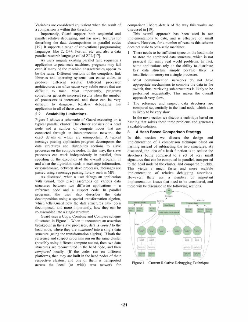
As users migrate existing parallel (and sequential) application to peta-scale machines, programs may fail even if many of the machine characteristics appear to be the same. Different versions of the compilers, link libraries and operating systems can cause codes to produce different results. Different processor architectures can often cause very subtle errors that are difficult to trace. Most importantly, programs sometimes generate incorrect results when the number of processors is increased, and these can be very difficult to diagnose. Relative debugging has application in all of these cases. 2.2 Scalability Limitations Figure 1 shows a schematic of Guard executing on a typical parallel cluster. The cluster consists of a head node and a number of compute nodes that are connected through an interconnection network, the exact details of which are unimportant. A typical message passing application program decomposes the data structures and distributes sections to slave processes on the compute nodes. In this way, the slave processes can work independently in parallel, thus speeding up the execution of the overall program. If and when the algorithm needs to exchange information, or synchronize, between slave processes, messages are passed using a message passing library such as MPI.

As discussed, when a user debugs an application with Guard, they place assertions on various data structures between two different applications – a reference code and a suspect code. In parallel programs, the user also describes the data decomposition using a special transformation algebra, which tells Guard how the data structures have been decomposed, and more importantly, how they can be re-assembled into a single structure.

Guard uses a Copy, Combine and Compare scheme illustrated in Figure 1. When it encounters an assertion breakpoint in the slave processes, data is copied to the head node, where they are combined into a single data structure (using the transformation algebra). If both the reference and suspect programs run on the same cluster (possibly using different compute nodes), then two data structures are reconstituted in the head node, and then compared locally. (If the codes run on different platforms, then they are built in the head nodes of their respective clusters, and one of them is transported across the local (or wide) area network for

comparison.) More details of the way this works are discussed in [19].

This overall approach has been used in our implementations to date, and is effective on small clusters. However, for a number of reasons this scheme does not scale to peta-scale machines: 1 There needs to be sufficient space on the head node

to store the combined data structure, which is not practical for many real world problems. In fact, some applications rely on the ability to distribute key data structure simply because there is insufficient memory on a single processor.

2 Most communication networks do not have appropriate mechanisms to combine the data in the switch, thus, retrieving sub-structures is likely to be performed sequentially. This makes the overall approach very slow.

3 The reference and suspect data structures are compared sequentially in the head node, which also is likely to be very slow. In the next section we discuss a technique based on

hashing that solves these three problems and generates a scalable solution. 3 A Hash Based Comparison Strategy In this section we discuss the design and implementation of a comparison technique based on hashing instead of subtracting the two structures. As discussed, the idea of a hash function is to reduce the structures being compared to a set of very small signatures that can be computed in parallel, transported to the head node of the cluster, and compared quickly. This yields a much faster and more scalable implementation of relative debugging assertions. However, there are a number of important implementation issues that need to be considered, and these will be discussed in the following sections.

Figure 1 – Current Relative Debugging Technique

121

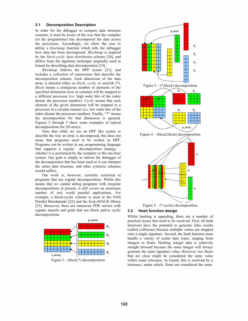
3.1 Decomposition Description In order for the debugger to compare data structure contents, it must be aware of the way that the compiler (or the programmer) has decomposed the data across the processors. Accordingly, we allow the user to define a blockmap function which tells the debugger how data has been decomposed. Blockmap is inspired by the block-cyclic data distribution scheme [20], and differs from the algebraic technique originally used in Guard for describing data decomposition [19].

Blockmap follows the HPF syntax [21], and includes a collection of expressions that describe the decomposition scheme. Each dimension of the data array is denoted either as block, cyclic or asterisk (*). Block means a contiguous number of elements of the specified dimension (row or column) will be mapped to a different processor (i.e. high order bits of the index dictate the processor number). Cyclic means that each element of the given dimension will be mapped to a processor in a circular manner (i.e. low order bits of the index dictate the processor number). Finally, “*” means the decomposition for that dimension is ignored. Figures 2 through 5 show some examples of typical decompositions for 2D arrays.

Note that while we use an HPF like syntax to describe the way an array is decomposed, this does not mean that programs need to be written in HPF. Programs can be written in any programming language that supports a regular decomposition strategy – whether it is performed by the compiler or the run-time system. Our goal is simply to inform the debugger of the decomposition that has been used so it can interpret the entire data structure, and other syntactic schemes would suffice.

Our work is, however, currently restricted to programs that use regular decompositions. Whilst this means that we cannot debug programs with irregular decompositions at present, it still covers an enormous number of real world parallel applications. For example, a block-cyclic scheme is used in the NAS Parallel Benchmarks [22] and the ScaLAPACK library [23]. Moreover, there are numerous PDE solvers with regular stencils and grids that use block and/or cyclic decompositions.

Figure 2 – (block,*) decomposition

Figure 3 – (*,block) decomposition

Figure 4 – (block,block) decomposition

Figure 5 – (*,cyclic) decomposition

3.2 Hash function design Whilst hashing is appealing, there are a number of practical issues that need to be resolved. First, all hash functions have the potential to generate false results (called collisions) because multiple values are mapped onto a single signature. Second, the hash function must handle a variety of scalar data types, ranging from integers to floats. Hashing integer data is relatively straight forward because the same integer will always generate the same signature value. However, two floats that are close might be considered the same value within some tolerance. In Guard, this is resolved by a tolerance, under which, floats are considered the same.

122

However, two slightly different floats will generate wildly different signatures, and thus a simple minded tolerance scheme cannot be implemented. Finally, the reference and suspect programs might invoke different numbers of processes, thus hashing the data held in each processor will generate different signatures even when the data is the same. Accordingly, we need to devise a hashing scheme that is insensitive to the number of processes. In the next three sessions, we deal with these challenges. 3.2.1 Desirable Hash Function Properties There are a number of good hashing functions and algorithms in practice that have been devised over the years [20, 21]. Each hashing function has a set of properties and designed goals. Here we compile a list of properties that suite data comparison purposes. In particular, the hashing function should: • minimise the number of collisions. This is important

because a high collision rate will indicate that arrays have the same contents when they don’t, and will confuse the debugging process.

• distribute signatures uniformly. • have an avalanche effect that ensures that the output

varies widely (e.g., half the bits changed) for a small change in input (e.g, changing a single bit). This is important because data may be skewed and only use a small part of the potential range of input values. This will allow us to detect changes even when data is skewed in this way.

• minimise the size of the signature. • detect permutations on data order within a structure.

This is important because index permutation is a common error when code is parallelised and evolved. (In applications that might wish to ignore permutations this attribute could be excluded from the desirable list or properties) According to [24], hash functions such as the Bob

Jenkins’ hash function, FNV hash functions, the SHA hash family, or the MD hash family all exhibit the above properties [24, 25], with advanced hashing evaluation and design techniques discussed in [26-28]. As a result, we have chosen Bob Jenkins’ hash function and FNV hash function, because they are relatively simple to implement, work consistently on different data types, and promise very efficient performance, while being hardware and platform independent.

Importantly, a recent application of Bob Jenkins’ function, for a similar application, suggests that the collision rate for real data sets might be as low as 2.3 * 10-10 when generating a 32 bit signature [29]. Further rsync [30] uses the MD5 hash functions to perform data synchronisation over the network. In this work, the authors argue that the collision probability is too low (2-160) to be nontrivial.

In spite of these results, we were concerned that even a small collision probability might make the scheme ineffective. Accordingly, we evaluated the probability of collisions in the FNV and Bob Jenkins’ hash functions to confirm their suitability for data comparisons. To match real world data conditions, we tested them with a range of data types including character string, short, signed/unsigned integer and floating points. The data was arranged in arrays, with different patterns such as random, skewed (increase/decrease incrementally in values), and permuted.

The total amount of data used in the evaluation was around 46GB, distributed into 150,000 pairs of data arrays. The choice of parameters for this evaluation is motivated by the case study discussed in Section 4. It represents the data structure size for a real application running on a peta-scale machine. Each array was hashed individually to generate one 64 bits hashed signature. The result of the experiment shows no collision at all.

In the unlikely event that the debugger misses detecting an error, it would likely be picked up slightly later in the execution, mitigating the effect of collisions even further. For example, data structures are often manipulated in loops, in which case the assertion fires multiple times. Thus, even if the assertion misses an error the first time a divergence occurred, it would almost certainly detect the error on the next loop iteration. 3.2.2 Floating Point precision As discussed, comparison tolerances allow floating point numbers to be considered equal if their magnitude of the difference is within the tolerance [19]. We have implemented both absolute and relative tolerances in the past and found them effective as a technique to remove insignificant differences in data. However, this scheme cannot be used in combination with hashing because hashing is performed on the source data before the two structures are combined.

An alternative way of masking insignificant changes is to use a slightly different definition of tolerance. Instead of subtracting two numbers, if we pre-round (or truncate) floating point values prior to comparison, then some of the low order digits will be removed before they are subtracted. Thus, two numbers that are close will round to the same number, and thus the hash values will be the same.

We note that, rounding is not the same as using a fixed tolerance. For example, given that we want to the numbers to be equal only to the nearest 0.001, consider the following floating point numbers: 0.1239, 0.1244, and 0.1245. Clearly, these round to 0.124, 0.124 and 0.125 respectively. Thus, the first two numbers will be considered within tolerance, but the latter two will not.

123

In spite of this difference, we have adopted this approach because it provides a tolerance-like behaviour and can be combined with hashing. In either scheme, the choice of tolerance is somewhat arbitrary and it an experimental parameter used at run time. In most cases users need to choose the error tolerance with an understanding of the application, because in some cases small errors are significant, and in others they should be ignored. 3.2.3 Decomposition Independence A simple minded implementation of hashing computes a single signature for the data held by each processor, combines and compares these in the head node. However, in order for this scheme to work, each of the programs must use the same number of processes and also identical data decomposition functions.

A solution to this problem involves evaluating multiple signatures per processor rather than one, and computing these in a way that is independent of the number of processors and decomposition strategy. By making the number of hash signatures returned by all processes the same in both programs, they can be compared directly. Definition. Let p denotes the number of processes in a parallel program. Let data(d1, d2, …, dn) denote the shape of an array. In this case n is the rank of the array and dn is the size of nth dimension of the array. For example, if A = data(100, 105), A is an array of rank 2 with 100 rows and 105 columns.

Let blockmap(A, m1, m2, … , mn) represents the decomposition function of an given array. For instance, given B = data(100, 105) then blockmap(B, 10, 105) indicates that the array B is decomposed into 10 sub arrays of shape (10,105). Accordingly, the following condition is held:

d1 * d2 * … * dn = p * (m1 * m2 * … * mn) Proposition. Given reference program R with pR processes and suspect program S with pS processes, assume both programs generate the data structure A of shape data(d1, d2, …, dn).

Suppose that R implements decomposition scheme blockmap1(A, b1, b2, … , bn) and S implements decomposition scheme blockmap2(A, c1, c2, … , cn). If hash_size(A, x1, x2, …, xn) is a function that takes an array of rank n and returns an array of hash signatures where each signature corresponds to a sub-array of shape (x1, x2, …, xn), then the formula to calculate xi (1!i!n) so that after hashing both programs end up with the exact same array of hash signatures is as follows:

xi = gcd(bi, ci) where function gcd(x,y) returns the most common divisor of x, y. In other words, we are

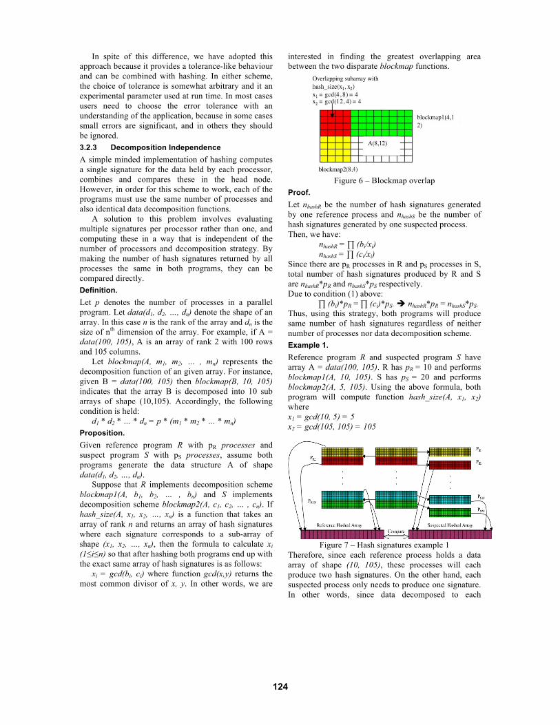
interested in finding the greatest overlapping area between the two disparate blockmap functions.

Figure 6 – Blockmap overlap

Proof. Let nhashR be the number of hash signatures generated by one reference process and nhashS be the number of hash signatures generated by one suspected process. Then, we have:

nhashR = " (bi/xi) nhashS = " (ci/xi)

Since there are pR processes in R and pS processes in S, total number of hash signatures produced by R and S are nhashR*pR and nhashS*pS respectively. Due to condition (1) above:

" (bi)*pR = " (ci)*pS. ! nhashR*pR = nhashS*pS. Thus, using this strategy, both programs will produce same number of hash signatures regardless of neither number of processes nor data decomposition scheme. Example 1. Reference program R and suspected program S have array A = data(100, 105). R has pR = 10 and performs blockmap1(A, 10, 105). S has pS = 20 and performs blockmap2(A, 5, 105). Using the above formula, both program will compute function hash_size(A, x1, x2) where x1 = gcd(10, 5) = 5 x2 = gcd(105, 105) = 105

Figure 7 – Hash signatures example 1

Therefore, since each reference process holds a data array of shape (10, 105), these processes will each produce two hash signatures. On the other hand, each suspected process only needs to produce one signature. In other words, since data decomposed to each

124

reference process is twice as much the data distributed to each suspected process, reference processes have to generate twice the number of signatures. Upon completion, it is expected that two arrays with shape (1, 20) of hash signatures will be compared directly at the client side. Example 2. Reference program R and suspected program S have an array A = data(100, 105). R has pR = 10 and performs blockmap1(A, 10, 105). S has pS = 7 and performs blockmap2(A, 100, 15). Using the above formula, both program will have to compute function hash_size(A, x1, x2) where x1 = gcd(10, 100) = 10 x2 = gcd(105, 15) = 15

As the result, since each reference process holds a data array of shape (10, 105) and function hash_size above maps one signature to a sub-array (10,15), each process produces 105/15=7 hash signatures. Similarly, each suspected process will need to produce 100/10=10 signatures.

However, after collecting the hashes from each program, we can see that R has a (7, 10) array of signatures while S has a (10, 7) array of signatures. Relevant Index Permutation [19] operation will be performed on 1 of the array so that 2 arrays of signatures of shape (10, 7) will be compared at the client side.

Figure 8 – Hash signatures example 2

Example 3 Reference program R and suspected program S have an array A = data(32, 50). R has pR = 8 and performs blockmap1(A, 4, 50). S has pS = 50 and performs blockmap2(A, 32, 1) (e.g (*,cyclic) distribution). Using the above formula, both program will have to compute function hash_size(A, x1, x2) where x1 = gcd(4, 32) = 4 x2 = gcd(50, 1) = 1

As the result, since each reference process holds a data array of shape (4, 1) and function hash_size above maps one signature to a sub-array (4,1), each reference process produces 50/1=50 hash signatures. Similarly, each suspected process will need to produce 32/4=8 signatures. As expected, a same amounts of hashed signatures produced by both programs. Upon collected, these signatures are arranged using the blockmap information into comparable signatures arrays.

Figure 9 – Hash signatures example 3

Efficiency The above strategy ensures that there is always an overlapped region between two arbitrary blockmap functions. However, if reference program and suspected program deploy blockmap functions such as (*, cyclic) and (cyclic, *), the overlapped region may be very small – in the limit, only a single cell. In this case hashing would add no value because each hash function would only hash one array element. On the other hand, it is unlikely that any parallel program would be efficient if it only allocated a single row or column to a given processor, and thus, we can assume that in any real program on any real machine there are likely to be multiple rows or columns assigned to a given processor. 3.3 Collecting Hash Signatures In order to collect the data from the processes as quickly as possible, we use collective operations similar to the broadcast and gather operations in MPI. (We remind readers that the processes will be stopped at breakpoints, and thus the state can be extracted using normal debugger functionality.) In particular, broadcast is used to request the debug processors to hash their data in parallel – all responding to a single broadcast command. Collective gather operations are used to merge signatures for comparison in the head node. This approach is quite scalable because, even though we compare the signatures sequentially in the head node, these are quite small, and the hashing operations, which can be time consuming, are performed in parallel.

Hashed block (4,1)

PR1

PS1

125

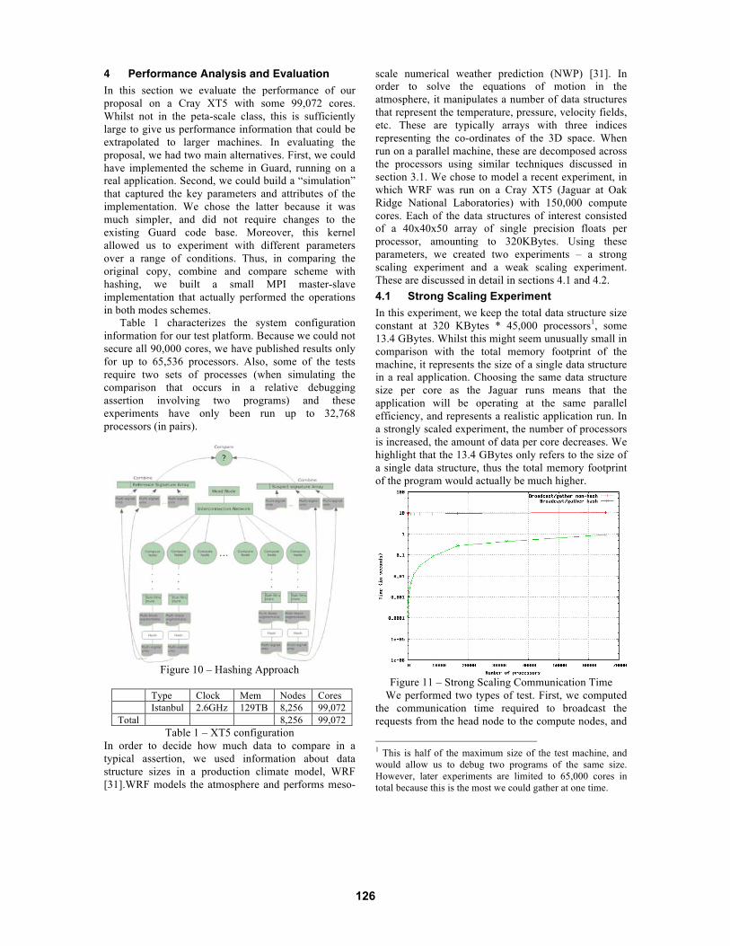
4 Performance Analysis and Evaluation In this section we evaluate the performance of our proposal on a Cray XT5 with some 99,072 cores. Whilst not in the peta-scale class, this is sufficiently large to give us performance information that could be extrapolated to larger machines. In evaluating the proposal, we had two main alternatives. First, we could have implemented the scheme in Guard, running on a real application. Second, we could build a “simulation” that captured the key parameters and attributes of the implementation. We chose the latter because it was much simpler, and did not require changes to the existing Guard code base. Moreover, this kernel allowed us to experiment with different parameters over a range of conditions. Thus, in comparing the original copy, combine and compare scheme with hashing, we built a small MPI master-slave implementation that actually performed the operations in both modes schemes.

Table 1 characterizes the system configuration information for our test platform. Because we could not secure all 90,000 cores, we have published results only for up to 65,536 processors. Also, some of the tests require two sets of processes (when simulating the comparison that occurs in a relative debugging assertion involving two programs) and these experiments have only been run up to 32,768 processors (in pairs).

Figure 10 – Hashing Approach

Type Clock Mem Nodes Cores Istanbul 2.6GHz 129TB 8,256 99,072 Total 8,256 99,072

Table 1 – XT5 configuration In order to decide how much data to compare in a typical assertion, we used information about data structure sizes in a production climate model, WRF [31].WRF models the atmosphere and performs meso-

scale numerical weather prediction (NWP) [31]. In order to solve the equations of motion in the atmosphere, it manipulates a number of data structures that represent the temperature, pressure, velocity fields, etc. These are typically arrays with three indices representing the co-ordinates of the 3D space. When run on a parallel machine, these are decomposed across the processors using similar techniques discussed in section 3.1. We chose to model a recent experiment, in which WRF was run on a Cray XT5 (Jaguar at Oak Ridge National Laboratories) with 150,000 compute cores. Each of the data structures of interest consisted of a 40x40x50 array of single precision floats per processor, amounting to 320KBytes. Using these parameters, we created two experiments – a strong scaling experiment and a weak scaling experiment. These are discussed in detail in sections 4.1 and 4.2. 4.1 Strong Scaling Experiment In this experiment, we keep the total data structure size constant at 320 KBytes * 45,000 processors1, some 13.4 GBytes. Whilst this might seem unusually small in comparison with the total memory footprint of the machine, it represents the size of a single data structure in a real application. Choosing the same data structure size per core as the Jaguar runs means that the application will be operating at the same parallel efficiency, and represents a realistic application run. In a strongly scaled experiment, the number of processors is increased, the amount of data per core decreases. We highlight that the 13.4 GBytes only refers to the size of a single data structure, thus the total memory footprint of the program would actually be much higher.

Figure 11 – Strong Scaling Communication Time

We performed two types of test. First, we computed the communication time required to broadcast the requests from the head node to the compute nodes, and

1 This is half of the maximum size of the test machine, and would allow us to debug two programs of the same size. However, later experiments are limited to 65,000 cores in total because this is the most we could gather at one time.

126

to transfer data from slave nodes back to the head node. This was done both with and without hashing, and allowed us to measure the difference in communication efficiency of the two schemes.

This data (Figure 11), shows that as the number of processors increases, the time for transferring the complete data is almost constant. This is not surprising, because data can only be received serially in the head node, and thus, regardless of the number of slave processes sending in parallel, the same amount of data is transferred. On the other hand, since the number of hash signatures increases with the number of processors, the time to transfer the signatures also increases. It is clear from this graph that transmitting hash signatures is much more efficient that transferring the entire data structure. This, of course, ignores the complication that it is unlikely that there is sufficient space for the whole data structure in the head node, in any event.

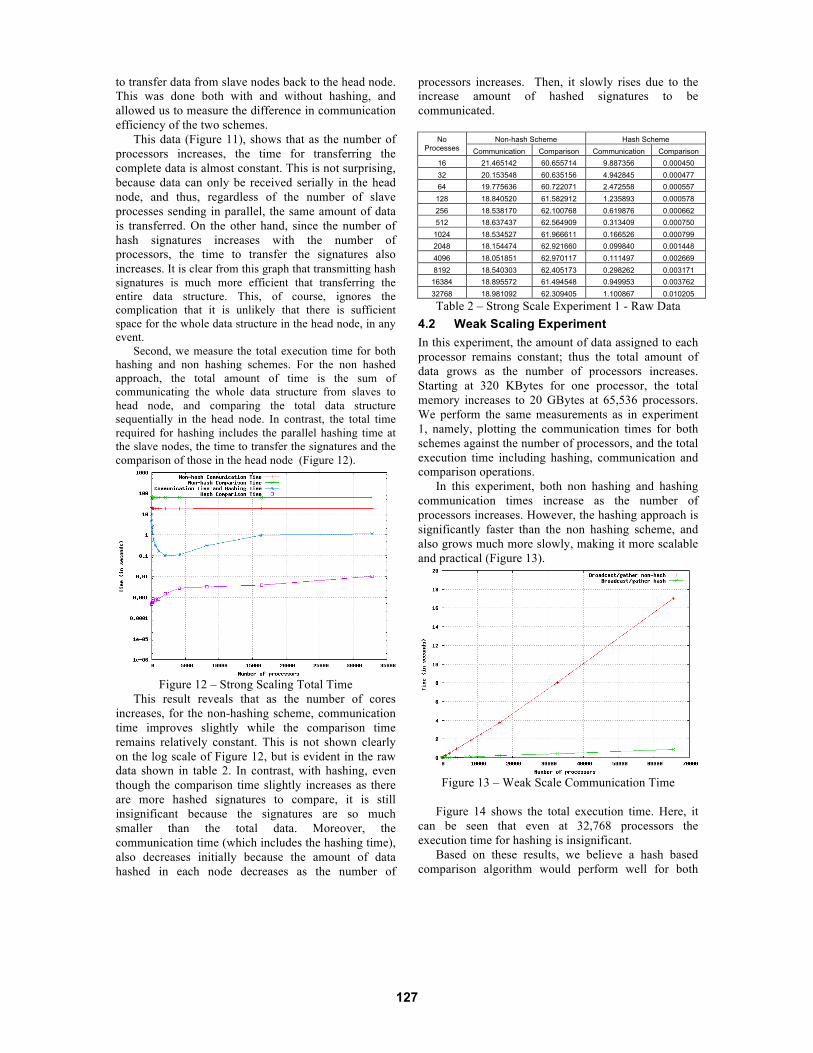
Second, we measure the total execution time for both hashing and non hashing schemes. For the non hashed approach, the total amount of time is the sum of communicating the whole data structure from slaves to head node, and comparing the total data structure sequentially in the head node. In contrast, the total time required for hashing includes the parallel hashing time at the slave nodes, the time to transfer the signatures and the comparison of those in the head node (Figure 12).

Figure 12 – Strong Scaling Total Time

This result reveals that as the number of cores increases, for the non-hashing scheme, communication time improves slightly while the comparison time remains relatively constant. This is not shown clearly on the log scale of Figure 12, but is evident in the raw data shown in table 2. In contrast, with hashing, even though the comparison time slightly increases as there are more hashed signatures to compare, it is still insignificant because the signatures are so much smaller than the total data. Moreover, the communication time (which includes the hashing time), also decreases initially because the amount of data hashed in each node decreases as the number of

processors increases. Then, it slowly rises due to the increase amount of hashed signatures to be communicated.

Non-hash Scheme Hash Scheme No

Processes Communication Comparison Communication Comparison 16 21.465142 60.655714 9.887356 0.000450 32 20.153548 60.635156 4.942845 0.000477 64 19.775636 60.722071 2.472558 0.000557

128 18.840520 61.582912 1.235893 0.000578 256 18.538170 62.100768 0.619876 0.000662 512 18.637437 62.564909 0.313409 0.000750

1024 18.534527 61.966611 0.166526 0.000799 2048 18.154474 62.921660 0.099840 0.001448 4096 18.051851 62.970117 0.111497 0.002669 8192 18.540303 62.405173 0.298262 0.003171

16384 18.895572 61.494548 0.949953 0.003762 32768 18.981092 62.309405 1.100867 0.010205

Table 2 – Strong Scale Experiment 1 - Raw Data 4.2 Weak Scaling Experiment In this experiment, the amount of data assigned to each processor remains constant; thus the total amount of data grows as the number of processors increases. Starting at 320 KBytes for one processor, the total memory increases to 20 GBytes at 65,536 processors. We perform the same measurements as in experiment 1, namely, plotting the communication times for both schemes against the number of processors, and the total execution time including hashing, communication and comparison operations.

In this experiment, both non hashing and hashing communication times increase as the number of processors increases. However, the hashing approach is significantly faster than the non hashing scheme, and also grows much more slowly, making it more scalable and practical (Figure 13).

Figure 13 – Weak Scale Communication Time

Figure 14 shows the total execution time. Here, it

can be seen that even at 32,768 processors the execution time for hashing is insignificant.

Based on these results, we believe a hash based comparison algorithm would perform well for both

127

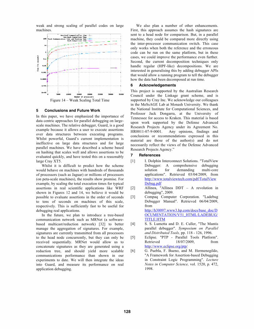
weak and strong scaling of parallel codes on large machines.

Figure 14 – Weak Scaling Total Time

5 Conclusions and Future Work In this paper, we have emphasized the importance of data centric approaches for parallel debugging on large-scale machines. The relative debugger, Guard, is a good example because it allows a user to execute assertions over data structures between executing programs. Whilst powerful, Guard’s current implementation is ineffective on large data structures and for large parallel machines. We have described a scheme based on hashing that scales well and allows assertions to be evaluated quickly, and have tested this on a reasonably large Cray XT5.

Whilst it is difficult to predict how the scheme would behave on machines with hundreds of thousands of processors (such as Jaguar) or millions of processors (on peta-scale machines), the results show promise. For example, by scaling the total execution times for typical assertions in real scientific applications like WRF shown in Figures 12 and 14, we believe it would be possible to evaluate assertions in the order of seconds to tens of seconds on machines of this scale, respectively. This is sufficiently fast to be useful for debugging real applications.

In the future, we plan to introduce a tree-based communication network such as MRNet (a software-based multicast/reduction network) [32] to better manage the aggregation of signatures. For example, signatures are currently transmitted from all processors to the head node concurrently, but they can only be received sequentially. MRNet would allow us to concatenate signatures as they are generated using a reduction tree, and should yield more scalable communications performance than shown in our experiments to date. We will then integrate the ideas into Guard, and measure its performance on real application debugging.

We also plan a number of other enhancements. First, this approach assumes the hash signatures are sent to a head node for comparison. But, in a parallel machine, they could be compared more directly using the inter-processor communication switch. This case only works when both the reference and the erroneous code can be run on the same platform, but in these cases, we could improve the performance even further. Second, the current decomposition techniques only handle regular (HPF-like) decompositions. We are interested in generalising this by adding debugger APIs that would allow a running program to tell the debugger how the data had been decomposed at run time. 6 Acknowledgements This project is supported by the Australian Research Council under the Linkage grant scheme, and is supported by Cray Inc. We acknowledge our colleagues in the MeSsAGE Lab at Monash University. We thank the National Institute for Computational Sciences, and Professor Jack Dongarra, at the University of Tennessee for access to Kraken. This material is based upon work supported by the Defense Advanced Research Projects Agency under its Agreement No. HR0011-07-9-0001. Any opinions, findings and conclusions or recommendations expressed in this material are those of the author(s) and do not necessarily reflect the views of the Defense Advanced Research Projects Agency.” 7 References [1] I. Dolphin Interconnect Solutions. "TotalView

Debugger: A comprehensive debugging solution for demanding multi-core applications". Retrieved 03/04/2009, from http://www.totalviewtech.com/pdf/TotalViewDebug.pdf

[2] Allinea, "Allinea DDT – A revolution in debugging", 2009.

[3] Compaq Computer Corporation. "Ladebug Debugger Manual". Retrieved 06/04/2009, from http://h30097.www3.hp.com/docs/base_doc/DOCUMENTATION/V51_HTML/LADEBUG/TITLE.HTM

[4] S. S. Lumetta and D. E. Culler, "The Mantis parallel debugger". Symposium on Parallel and Distributed Tools, pp. 118 - 126, 1996.

[5] Eclipse. "PTP - Parallel Tools Platform". Retrieved 18/07/2009, from http://www.eclipse.org/ptp/

[6] G. Puebla, F. Bueno, and M. Hermenegildo, "A Framework for Assertion-based Debugging in Constraint Logic Programming". Lecture Notes in Computer Science, vol. 1520, p. 472, 1998.

128

[7] W. Drabent, S. Nadjm-Tehrani, and J. Maluszynski, "Algorithmic debugging with assertions" in Meta-programming in logic programming: MIT Press, 1989, pp. 501 - 521.

[8] M. Auguston, C. Jeffery, and S. Underwood, "A Framework for Automatic Debugging" in Automated Software Engineering, 2002, pp. 217-222.

[9] Sun Microsystems. "Programming With Assertions". Retrieved 20/06/2009, from http://java.sun.com/j2se/1.4.2/docs/guide/lang/assert.html

[10] P. Horan, "Eiffel Assertions and the External Structure of Classes and Objects". Journal of Object Technology, vol. 1, pp. 105-118, 2002.

[11] M. A. Marin, "Effective use of assertions in C++". ACM SIGPLAN Notices, vol. 31, pp. 28 - 32, 1996.

[12] R. E. Fairley, "ALADDIN: Assembly language assertion driven debugging interpreter". IEEE TRANSACTIONS ON SOFTWARE ENGINEERING, vol. 5, pp. 426- 428, 1979.

[13] R. Sosic and D. Abramson, "Guard: A relative debugger". Software Practice and Experience, vol. 27, pp. 94-115, 1997.

[14] D. Abramson, G. Watson, and L. P. Dung, "Guard: A Tool for Migrating Scientific Applications to the .NET Framework". Lecture Notes in Computer Science, vol. 2330, pp. 834-843, 2002.

[15] D. Abramson, I. Foster, J. Michalakes, and R. Sosic, "Relative Debugging - A new methodology for debugging scientific applications". Communications of the ACM, vol. 39, pp. 69-77, 1996.

[16] D. Abramson, I. Foster, J. Michalakes, and R. Sosic, "Relative debugging and its application to the development of large numerical models" in Conference on High Performance Networking and Computing San Diego, California: ACM, 1995.

[17] G. Watson and D. Abramson, "Relative Debugging for Data-Parallel Programs: A ZPL Case Study". IEEE Concurrency, vol. 8, pp. 42-52, 2000.

[18] G. Watson and D. Abramson, "Parallel Relative Debugging for Distributed Memory Applications: A Case Study" in International Conference on Parallel and Distributed Processing Techniques and Applications Las Vegas, Nevada, USA, 2001.

[19] G. R. Watson, "The Design and Implementation of a Parallel Relative Debugger". PhD Thesis, Faculty of

Information Technology, Monash University, 2000

[20] A. Petitet. "Block Cyclic Data Distribution". Retrieved 20/12/2009, from http://www.netlib.org/utk/papers/scalapack/node8.html

[21] H. Richardson, "High Performance Fortran: history, overview and current developments", Thinking Machines Corporation, 1996.

[22] NASA Advanced Supercomputing Division. "NAS PARALLEL BENCHMARKS". Retrieved 20/12/2009, from http://www.nas.nasa.gov/Resources/Software/npb.html

[23] ScaLAPACK Project. "The ScaLAPACK Project". Retrieved 21/12/2009, from http://www.netlib.org/scalapack/index.html

[24] B. Mulvey. "Hash Functions". Retrieved 26/03/2009, from http://bretm.home.comcast.net/~bretm/hash/

[25] S. Bakhtiari, R. Safavi-Naini, and J. Pieprzyk, "Cryptographic Hash Functions: A Survey". 1995.

[26] P. Wolper and D. Leroy, "Reliable Hashing without Collision Detection". Lecture Notes in Computer Science, vol. 697, pp. 59-70, 1993.

[27] I. Mironov, "Hash Functions: Theory, attacks, and applications", Microsoft Research, Silicon Valley Campus, 2005.

[28] G. D. Knott, "Hashing Functions". Computer Jounal, vol. 18, pp. 265-278, 1972.

[29] M. Molina, S. Niccolini, and N. G. Duffield., "A Comparative Experimental Study of Hash Functions Applied to Packet Sampling" in International Teletraffic Congress (ITC-19), 2005.

[30] A. Tridgell, "Efficient Algorithms for Sorting and Synchronization". PhD Thesis, The Australian National University, 1999

[31] J. Michalakes, J. Hacker, R. Loft, M. O.McCracken, A. Snavely, and N.-l. J. Wright, "WRF Nature Run" in High Performance Networking and Computing Nevada: ACM, 2007.

[32] P. C. Roth, D. C. Arnold, and B. P. Miller, "MRNet: A Software-based Multicast/Reduction Network for Scalable Tools" in Proceedings of SC, Phoenix, AZ, 2003.

129