The Canadian Journal of Statistics

Vol. 34, No 2, 2006, Pages ???–???

La revue canadienne de statistique

A Bayesian signal detection procedure for scale-space random fields

M. Farid ROHANI, Khalil SHAFIE and Siamak NOORBALOOCHI

Key words and phrases: Bayes factor; scale space random fields; signal detection.MSC 2000 : Primary 60G60; 62M40; Secondary 62F15; 60D05.

Abstract: The authors consider the problem of searching for activation in brain images obtained from

functional magnetic resonance imaging and the corresponding functional signal detection problem. They

develop a Bayesian procedure to detect signals existing within noisy images when the image is modeled

as a scale space random field. Their procedure is based on the Radon–Nikodym derivative, which is used

as the Bayes factor for assessing the point null hypothesis of no signal. They apply their method to data

from the Montreal Neurological Institute.

Une procedure bayesienne de detection de signal en champs aleatoiresa espace d’echelle

Resume : Les auteurs s’interessent au reperage de l’activation cerebrale a partir d’imagerie fonctionnellepar resonnance magnetique et au probleme de detection du signal fonctionnel afferent. Ils developpentune procedure bayesienne permettant de detecter un signal present dans des images bruitees modelisees enchamps aleatoires a espace d’echelle. Leur procedure s’appuie sur une derivee de Radon–Nikodym qui sertde facteur de Bayes dans l’evaluation de l’hypothese nulle d’absence de signal. Ils illustrent leur methodeau moyen de donnees provenant de l’Institut neurologique de Montreal.

1. INTRODUCTION

Magnetic resonance imaging (MRI) is a procedure that uses radio waves and a strong atomic mag-netic field rather than x-rays to provide images of internal organs that contrast significantly withsurrounding tissues. This technique, in addition to allowing neurologists to distinguish betweengray and white matter, and brain defects such as tumours, can be used to produce a large numbersof images in a short interval of time to produce a nearly continuous collection of images capturingrapid internal changes. Functional magnetic resonance imaging (FMRI) uses this capability ofthe MR imaging to measure the metabolic changes that take place in an active part of the brain.Even though the general areas of the brain where speech, sensation, memory, and other functionsoccur are known, their exact locations vary from individual to individual. Injuries and disease,such as concussions and brain tumours, can cause these functions to shift to other areas of thebrain. Because FMRI can quickly detect and identify signals, it can be used to determine whichlocations of the brain are handling these functions. Such information is obviously very critical forpathologists and developing interventions to treat central nervous system disorders.

In 1991, the first experiment using MRI was designed to study brain function. The experimentinvolved the imaging of the visual cortex while the subject was presented with a visual stimulus(Kwong et al. 1992). In a similar experiment at the Montreal Neurological Institute, a subject wasgiven a simple visual stimulus, flashing red dots, presented through light-light goggles (Ouyang,Pile & Evans 1994). The stimulus was switched off for 4 scans, then on for 4 scans. This procedure

1

was repeated 5 times, resulting in a total of 40 scans. The period between scans was 6 secondsand the stimulus period was 48 seconds. Hence, the data set consists of a time series of 40 two-dimensional images, each 128 × 128 pixels of size 2 mm. Our aim is to determine whether theactive vision component of the brain can be detected in the image area specified by our prior.

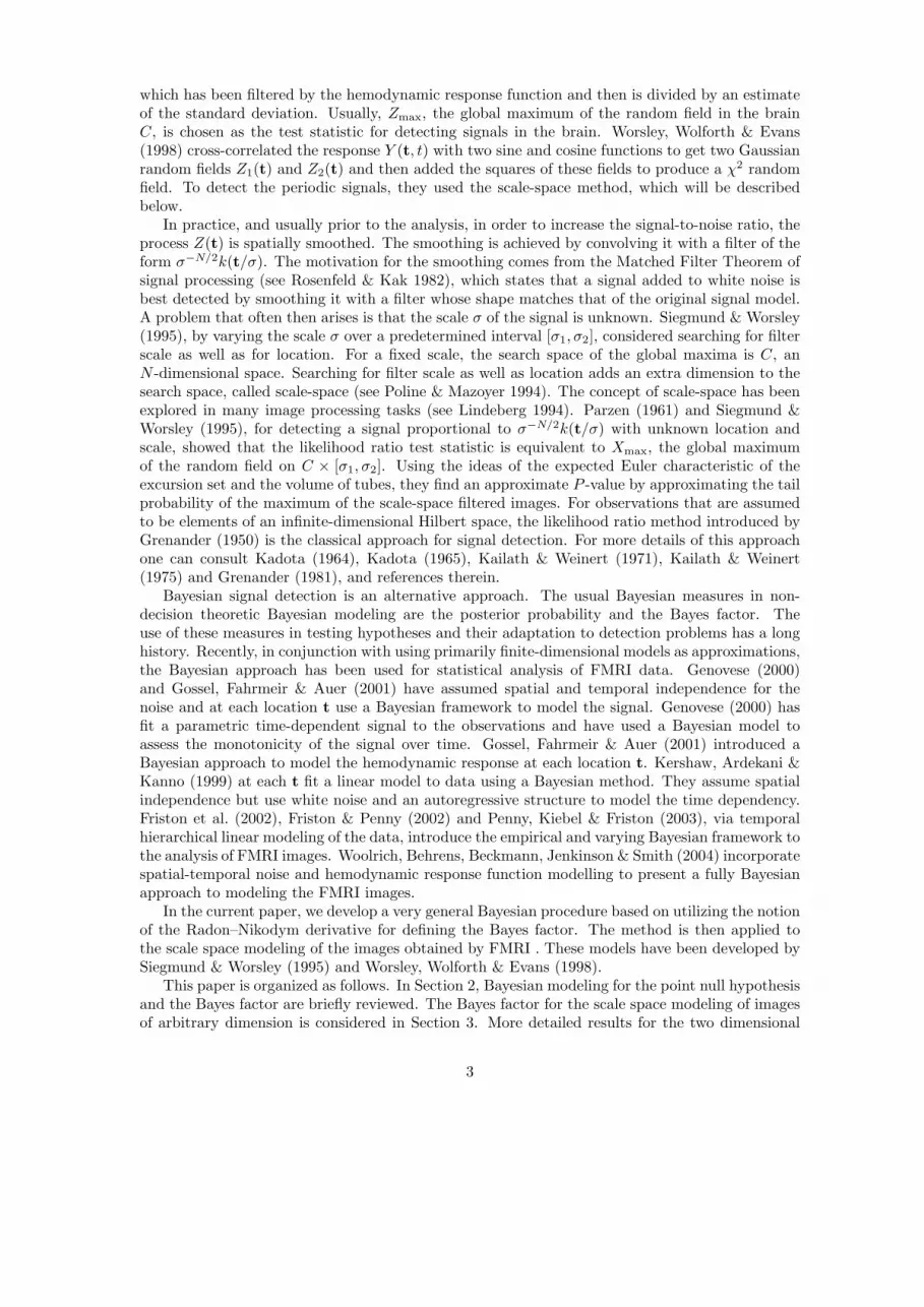
In this paper, we first fit a linear model at each pixel in sine and cosine waves with a periodmatching that of the stimulus. The coefficients of these two components, normalized to have unitvariance, are referred to as the sine and cosine components of the data. The phase was chosen sothat we expect the whole signal to be in the cosine component, whereas the sine component shouldhave no signal (zero mean). Shafie (1998), Worsley (2001) and Shafie, Sigal, Siegmund & Worsley(2003) have shown that most of the signal characteristics are preserved in the cosine componentthat approximates a Gaussian random field (see Figure 1). Hence, in the sequel, the question ofexistence of any signal will be studied using this component.

Figure 1: Cosine component of the real FMRI image

As usual, the desired information consists of signals enmeshed in noise, and prior to any criticaluse, statistical processing and analysis should be used to detect and interpret these signals.

An important task regarding the images obtained using FMRI or other modern sensor technolo-gies is to locate the isolated regions of the brain where activation occurs (the signal), and then toseparate these regions from the rest of the brain where no activation can be detected (the noise).In the present article, we apply our method to the data collected in the Montreal experimentdescribed above to see if we can detect an existing signal.

Formally, during an FMRI experiment, a sequence of brain images is obtained while the subjectis given a stimulus. At each time point t the subject is presented with a stimulus s(t) and theblood flow response Y (t, t) is measured at a spatial location t, where t ∈ C ⊂ RN and t ∈ T ={t1, . . . , tn}. The spatial-temporal response process Y (t, t) usually is modeled as a sum of twocomponents: the signal (the hemodynamic response), and the noise.

Depending on the aim of a study, different models have been proposed for statistical analysis ofFMRI data. Friston, Jezzard & Turner (1994), Friston et al. (1995) and Worsley & Friston (1995)modeled the signal component at a fixed location t as the convolution of s(t) with the hemodynamicresponse function which was modeled as a Gaussian function. The noise component was assumedto be a stationary spatio-temporal Gaussian process. Random field modeling of spatial processesis a common choice. Worsley, Evans, Marrett & Neelin (1992) and Worsley (1994), for signaldetection problems, have modeled the FMRI images of the brain as a Gaussian random field Z(t).To produce a Gaussian random field, Z(t), for FMRI data, Y (t, t) is cross-correlated with s(t),

2

which has been filtered by the hemodynamic response function and then is divided by an estimateof the standard deviation. Usually, Zmax, the global maximum of the random field in the brainC, is chosen as the test statistic for detecting signals in the brain. Worsley, Wolforth & Evans(1998) cross-correlated the response Y (t, t) with two sine and cosine functions to get two Gaussianrandom fields Z1(t) and Z2(t) and then added the squares of these fields to produce a χ2 randomfield. To detect the periodic signals, they used the scale-space method, which will be describedbelow.

In practice, and usually prior to the analysis, in order to increase the signal-to-noise ratio, theprocess Z(t) is spatially smoothed. The smoothing is achieved by convolving it with a filter of theform σ−N/2k(t/σ). The motivation for the smoothing comes from the Matched Filter Theorem ofsignal processing (see Rosenfeld & Kak 1982), which states that a signal added to white noise isbest detected by smoothing it with a filter whose shape matches that of the original signal model.A problem that often then arises is that the scale σ of the signal is unknown. Siegmund & Worsley(1995), by varying the scale σ over a predetermined interval [σ1, σ2], considered searching for filterscale as well as for location. For a fixed scale, the search space of the global maxima is C, anN -dimensional space. Searching for filter scale as well as location adds an extra dimension to thesearch space, called scale-space (see Poline & Mazoyer 1994). The concept of scale-space has beenexplored in many image processing tasks (see Lindeberg 1994). Parzen (1961) and Siegmund &Worsley (1995), for detecting a signal proportional to σ−N/2k(t/σ) with unknown location andscale, showed that the likelihood ratio test statistic is equivalent to Xmax, the global maximumof the random field on C × [σ1, σ2]. Using the ideas of the expected Euler characteristic of theexcursion set and the volume of tubes, they find an approximate P -value by approximating the tailprobability of the maximum of the scale-space filtered images. For observations that are assumedto be elements of an infinite-dimensional Hilbert space, the likelihood ratio method introduced byGrenander (1950) is the classical approach for signal detection. For more details of this approachone can consult Kadota (1964), Kadota (1965), Kailath & Weinert (1971), Kailath & Weinert(1975) and Grenander (1981), and references therein.

Bayesian signal detection is an alternative approach. The usual Bayesian measures in non-decision theoretic Bayesian modeling are the posterior probability and the Bayes factor. Theuse of these measures in testing hypotheses and their adaptation to detection problems has a longhistory. Recently, in conjunction with using primarily finite-dimensional models as approximations,the Bayesian approach has been used for statistical analysis of FMRI data. Genovese (2000)and Gossel, Fahrmeir & Auer (2001) have assumed spatial and temporal independence for thenoise and at each location t use a Bayesian framework to model the signal. Genovese (2000) hasfit a parametric time-dependent signal to the observations and have used a Bayesian model toassess the monotonicity of the signal over time. Gossel, Fahrmeir & Auer (2001) introduced aBayesian approach to model the hemodynamic response at each location t. Kershaw, Ardekani &Kanno (1999) at each t fit a linear model to data using a Bayesian method. They assume spatialindependence but use white noise and an autoregressive structure to model the time dependency.Friston et al. (2002), Friston & Penny (2002) and Penny, Kiebel & Friston (2003), via temporalhierarchical linear modeling of the data, introduce the empirical and varying Bayesian framework tothe analysis of FMRI images. Woolrich, Behrens, Beckmann, Jenkinson & Smith (2004) incorporatespatial-temporal noise and hemodynamic response function modelling to present a fully Bayesianapproach to modeling the FMRI images.

In the current paper, we develop a very general Bayesian procedure based on utilizing the notionof the Radon–Nikodym derivative for defining the Bayes factor. The method is then applied tothe scale space modeling of the images obtained by FMRI . These models have been developed bySiegmund & Worsley (1995) and Worsley, Wolforth & Evans (1998).

This paper is organized as follows. In Section 2, Bayesian modeling for the point null hypothesisand the Bayes factor are briefly reviewed. The Bayes factor for the scale space modeling of imagesof arbitrary dimension is considered in Section 3. More detailed results for the two dimensional

3

case are explained in Section 4. In Section 5, the Bayes factor is calculated for the previouslydescribed Montreal two-dimensional FMRI data set. The necessary classical results on Hilbert-valued Gaussian measures, their equivalences, a brief review of the Radon–Nikodym derivativecalculation and the technical proofs of the results are in the Appendix.

2. THE BAYES FACTOR OF A POINT NULL HYPOTHESIS

The Bayes factor has been defined as the ratio of the posterior odds ratio of the null hypothesisto the alternative over the corresponding prior odds ratio. Suppose X is an observable quantitywith density f(x|θ), where θ, the parameter of interest , and X both are elements of the Euclidianspace RN . Assume we are interested in assessing H0 : θ = θ0 against H1 : θ 6= θ0 and the prior isa two-stage prior (see Jeffreys 1961). Let π0 = P (H0) be the prior probability assigned to H0 anddefine the prior probability over Θ to be

π(θ) ={

π0, θ = θ0,(1− π0)g(θ), θ 6= θ0,

where given the alternative, g(θ) is a conditional prior probability over the alternative values. TheBayes factor for assessing a null hypothesis H0 against an alternative H1 generally is defined as

B(x) =P(H0|x)P(H1|x)

÷ P(H0)P(H1)

.

If g(θ) is a continuous density on {θ ∈ Θ : θ 6= θ0}, it is easy to see that for the above sharpnull testing problem, the Bayes factor is equivalent to B(x) = f(x|θ0)/mg(x), where

mg(x) =∫

f(x|θ)g(θ)dθ.

This factor incorporates prior information with the sample information in the likelihood. It can bethought of as the weighted likelihood ratio of H0 to H1. For arguments justifying the use of thisrelative measure in scientific inference problems, see Berger (1985) and Kass & Raftery (1995),which are among the more classical references.

Let (Θ,F2, G) be the prior probability space and for any θ ∈ Θ, let Pθ be a probability measureon (X ,F1). Suppose further that, for every B ∈ F1, Pθ(B) as a function of θ is an F2-measurablefunction. Here, F1 and F2 are corresponding σ-fields.

In the following, we essentially show how the computation of the Bayes factor can be reducedto the evaluation of the Radon–Nikodym derivative between two equivalent measures. We willdetail the computation of the factor for two equivalent Gaussian measures, which will be appliedto our image data in the next section.

LetPG(A) =

∫

Θ

Pθ(A)G(dθ)

be the marginal probability measure of X on (X ,F1). Then for a given θ0 ∈ Θ, Pθ0(A) andPG(A) are both probability measures on (X ,F1). The Lebesgue decomposition theorem ensuresthe existence of a set A0 ∈ F1 with PG(A0) = 0, such that for every A ∈ F1, ν0(A) = Pθ0(A∩A0)and ν1(A) = Pθ0(A∩ A0) where ν0 and PG are mutually singular, ν1 is absolutely continuous withrespect to PG, and Pθ0(A) = ν1(A) + ν0(A). Therefore, based on the Radon–Nikodym theorem,there exists a nonnegative PG-measurable function f such that for any set A ∈ F1 we have

Pθ0(A) =∫

A

f(x)PG(dx) + Pθ0(A ∩A0).

4

The Radon–Nikodym derivative of Pθ0 with respect to PG, will be denoted by f(x) = dPθ0/dPG(x).In this general setting, for testing H0 : θ = θ0 against H1 : θ 6= θ0, we can define the Bayes factoras

B(x) ={ ∞ , x ∈ A0,

f(x), x /∈ A0.(1)

Two extreme cases may occur. If the set A0 has Pθ0(A0) = 1, then the two measures PG and Pθ0

are perpendicular to each other and in this case A0 is the critical region that will allow us withoutany error to discriminate between H0 and H1. If Pθ0 and PG are equivalent, hence Pθ0(A0) = 0and f 6= 0 with PG-probability 1. In this case, based on a theorem by Grenander (1981), A0 andf can be found simultaneously. Lemma 1 (see Appendix) states the equivalence of the marginalmodel with all the conditional (given θ) models. The Bayes factor in (1) can then be obtained asis stated in the following theorem, the proof of which is in Appendix.

Theorem 1. Under the conditions of Lemma 1, there exists A0 ∈ F1 with PG(A0) = 0, such thatthe Bayes factor for testing H0 : θ = θ0 versus H1 : θ 6= θ0 comes from

B(x) =

∞ , x ∈ A0;

1/ {∫

dPθ

dPθ0

(x)dG(θ)}

, x /∈ A0.

3. THE BAYES FACTOR FOR THE SCALE SPACE RANDOM FIELDS

Consider the random field Z(t), where t ∈ RN satisfies

dZ(t) = ξσ−N/20 f

{σ−1

0 (t− t0)}

dt + dW (t),

where t0 ∈ C, ξ ≥ 0 and σ0 > 0, are fixed values and dW is a white noise. The unknown parameter(ξ, t0, σ0) represents the amplitude, location, and scale of a signal added to the white noise dW (t).Here, f is an N -dimensional shape function.

Let k be an N -dimensional kernel such that∫

k(t)2dt = 1. (2)

An important choice for the kernel function is the Gaussian form,

k(t) = π−N/4 exp(−||t||2/2).

For kernel function k, Siegmund & Worsley (1995) define the Gaussian scale space random fieldas

X(t, σ) = σ−N/2

∫k

{σ−1(h− t)

}dZ(h).

Thus the general form of a Gaussian scale space random field is

X(t, σ) = (σ0σ)−N/2ξ

∫f

{σ−1

0 (h− t0)}

k{σ−1(h− t)

}dh (3)

+ σ−N/2

∫k

{σ−1(h− t)

}dW (h),

5

or if we denote the first and the second terms in (3) respectively by µ and W ∗, then

X(t, σ) = µ(t, σ ; ξ, t0, σ0) + W ∗(t, σ), (4)

where ξ, t0 = (t01, . . . , t0N ), and σ0 are unknown parameters, σ is the scale parameter of the kernelfunction, and W ∗(t, σ) is an N -dimensional Gaussian random field. We assume the unknownparameter θ = (ξ, t0, σ0) ∈ Θ = {(ξ, t0, σ0); ξ > 0, t0 ∈ C ⊆ RN , σ0 ∈ S ⊆ (0,∞)}.

The following lemma gives the mean and covariance functions of W ∗(t, σ) (see Siegmund &Worsley 1995).

Lemma 2. Let dW (t) be a white noise and k a kernel that satisfies (2), then

W ∗(t, σ) = σ−N/2

∫k

{σ−1(h− t)

}dW (h)

is an N -dimensional Gaussian random field with zero mean, unit variance, and covariance functionof the form

(σ1σ2)−N/2

∫k

{σ−1

1 (h− t1)}

k{σ−1

2 (h− t2)}

dh. (5)

Another model that we will consider is the following

X(t) = µ(t; θ) + W (t), (6)

where

µ(t; θ) = σ−N/20 ξ

N∏

i=1

∫

Ti

fi

(hi − t0i

σ0

)dhi

for some arbitrary functions, fis, i = 1, . . . , N on RN+ and W (t) is a Brownian sheet on RN

+ . Sincewe do not use any smoothing procedure for this case, we call this random field (6) a non-smoothGaussian scale space random field.

The Matched Filter Theorem of signal processing states that a signal added to white noise isbest detected by smoothing the white noise with a filter whose shape matches that of the signal.When the shape of the signal, f , is known, it is recommended that the image be smoothed usinga kernel the same as f . In this case, using the results on Gaussian measures on Hilbert spaces,we can calculate the Bayes factor. To do this, let H = L2(C, m) be the Hilbert space of squareintegrable functions on C, where m is Lebesgue measure on C, and let Pµ = HN(µ, ρ) be aGaussian measure on H with the mean µ and covariance operator ρ (see Appendix). In the casewhere µ = ξg(t, σ; t0, σ0), the test of no signal is equivalent to H0 : ξ = 0 against H1 : ξ > 0.Hence, for the Bayes factor we have the following result, where the proof of which is based onTheorem 7A of Parzen (1963).

Lemma 3. Let X(t) be the scale space Gaussian random field in (4), where t ∈ RN , and assumek = f . Then for testing the null hypothesis H0 : ξ = 0 against the alternative H1 : ξ = ξ∗, thelog-likelihood ratio test is equivalent to

ξ∗x(t0, σ0)− ξ∗2/2.

Under model (4), we obtain the following theorem as an immediate consequence of Theorems 1,4, 6 and Lemma 3.

6

Theorem 2. Under the conditions of Lemma 3, using the scale space Gaussian random field in(4), and testing H0 : ξ = 0 against H1 : ξ > 0, if µ(t, σ ; θ) ∈ R(ρ1/2) for θ = (ξ, t0, σ0), then P0

and PG are equivalent and the Bayes factor has the form

B(x) =

{ ∞ , x ∈ A0;1/ {∫

fθ(x)dG(θ)}

, x /∈ A0,(7)

where fθ(x) = exp{ξx(t0, σ0)− ξ2/2

}and A0 is such that PG(A0) = 0.

We can also obtain the Bayes factor for the non-smooth scale space random field (6) definedon a compact set C ⊂ RN

+ , using Theorems 1 and 6 as follows.

Theorem 3. For testing H0 : ξ = 0 against H1 : ξ > 0, if µ(t; θ) ∈ R(ρ1/2), in the non-smoothscale space Gaussian random field on a compact subset C of RN

+ , then P0 and PG are equivalentand

B(x) =dP0

dPG=

{∫

Θ

fθ(x)dG(θ)}−1

,

where

fθ(x) = exp

[ ∞∑

i=1

< ei, µ(.; θ) >

λi

{< x, ei > −< ei, µ(.; θ) >

2

}],

ei and λi, (i = 1, 2, . . .) are eigenfunctions and their corresponding eigenvalues of ρ, and < ·, · >denotes the inner product in the Hilbert space.

4. THE TWO-DIMENSIONAL CASE

In this section, we apply the results of the previous sections to a two-dimensional case. For simplic-ity, let θ = (ξ, t01, t02, σ0) and x = x(t01, t02, σ0). For a given x and a prior distribution function Gfor θ, we may use numerical integration techniques to calculate the Bayes factor. We assume that ξis independent of the other parameters (t01, t02, σ0), and has the improper distribution proportionalto Lebesgue measure on (0,∞), in other words, dG(θ) = dξ dG1(t01, t02, σ0).

First, we consider the case where

X(t, σ) = µ(t, σ; θ) + W ∗(t, σ), t ∈ C = [0, 1]× [0, 1], (8)

in whichµ(t, σ; θ) = (σ0σ)−N/2ξ

∫f

{σ−1

0 (h− t0)}

f{σ−1(h− t)

}dh,

andW ∗(t, σ) = σ−N/2

∫f

{σ−1(h− t)

}dW (h)

is a 2-dimensional Gaussian random field with zero mean, unit variance, and a covariance functionas defined in (5). Now, using (7) we obtain the Bayes factor as follows (details of computationsare in the Appendix):

B(x) ={∫

Φ(x)φ(x)

dG1(t01, t02, σ0)}−1

, (9)

where φ and Φ denote the density and distribution functions of the standard Gaussian distribution,respectively. It is not difficult to see that this Bayes factor satisfies the following inequalities

φ(x)Φ(x)

≤ B(x) ≤ 1√2πΦ(x)

,

7

where x and x are global maxima and minima of x, respectively.Now consider the non-smooth random field

X(t) = µ(t; θ) + W (t), t ∈ C = [0, 1]× [0, 1], (10)

where

µ(t; θ) = σ−10 ξ

{∫ t1

0

f1

(h1 − t01

σ0

)dh1

} {∫ t2

0

f2

(h2 − t02

σ0

)dh2

}

and W is the Brownian sheet on C.We know that the eigenvalues λi and the corresponding eigenfunctions ϕi(t) of the Brown-

ian motion on [0, 1] are 1/{(i + 1/2)2π2} and√

2 sin{(i + 1/2)πt}, respectively (see Gikhman &Skorokhod 1969, p. 189). It is not hard to see that the eigenvalues and the eigenfunctions ofρ{(t1, t2), (s1, s2)} = min(s1, t1)×min(s2, t2) are

λij =1

(i + 1/2)2(j + 1/2)2π4, ϕij(t1, t2) = 2 sin{(i + 1/2)πt1} sin{(j + 1/2)πt2},

respectively.To find the Bayes factor from Theorem 3, we need to calculate two inner products < x, ϕij >

and < ϕij , µ >. The detailed calculation of the inner products and the corresponding Bayes factorare given in the Appendix. The final computed Bayes factor that we are going to use in the thenext section is given by

B(x) =

∫1√E

Φ(D/√

E)

φ(D/√

E) dG1(t01, t02, σ0)

−1

, (11)

where

D =∞∑

i=1

∞∑

j=1

< ϕij , η) >< x, ϕij >

λijand E =

∞∑

i=1

∞∑

j=1

< ϕij , η >2

λij,

and η is defined in (13).

5. APPLICATION TO FMRI

In this section we will use the methodology developed in the previous sections to the MontrealNeurological Institute FMRI scans reported by Ouyang, Pile & Evans (1994).

Different classical methods, based on random field modeling or otherwise, have been usedto analyze this data. For the random field modeling, Worsley (2001) has applied the χ2 scalespace random field approach, and Shafie, Sigal, Siegmund & Worsley (2003) have utilized therotation space random field method for detection. Both methodologies are based on computingan approximate P -value. Here, we will apply the Bayes factor method to the scale space model ofSiegmund & Worsley (1995). The Bayes factor will be approximated under different sets of priorsand the robustness of the factor with respect to the choice of super parameters will be explored.

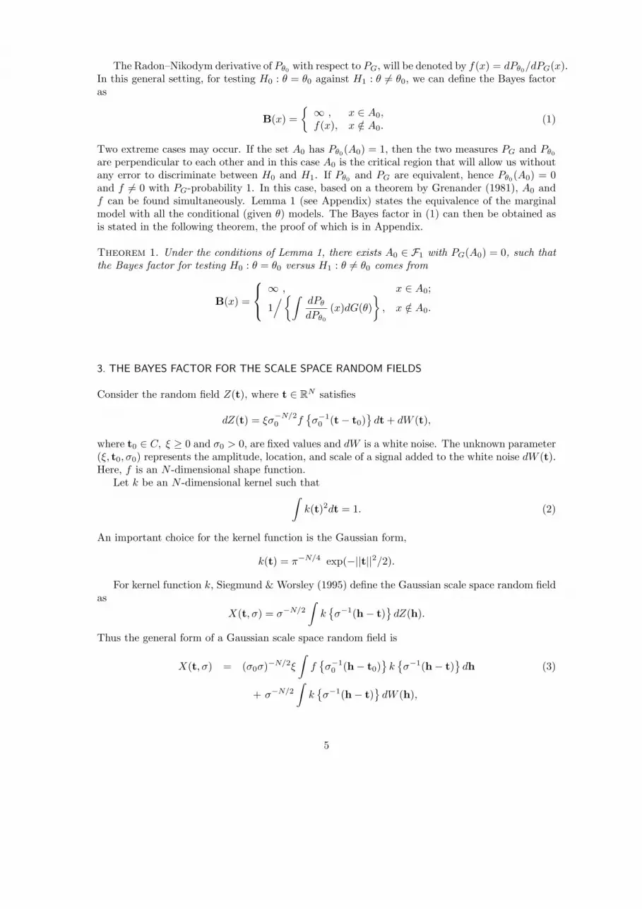
As stated before, when the shape of the signal is known, it is recommended to smooth theimage before any analysis. Figure 2 shows a smoothed version of the image. After smoothing theimage, we can apply model (8), and results of the previous section for signal detection. First, wenote that in our example the global maximum of the random field is 18.92 for σ ∈ [0, 1], where thismaximum occurs at (σ, t1, t2) = (1, .535, .252).

Now, given a prior distribution for parameters, we can compute the Bayes factor for weighingour hypothesis according to (9). A critical feature of any Bayesian analysis is the choice of a prior.If one has detailed information about the possible parameter values, the use of subjective priors

8

Figure 2: A smoothed version of the FMRI image

reflecting this information is justifiable. However, in practice this is not always the case and notenough information exists to form the prior. Even in the presence of such information, tryingto find a suitable prior that properly incorporates the researcher’s prior belief into the analysismay require considerable effort. Finally, even in the presence of satisfactory information andability to model this information through proper priors, the classical controversy of the subjectiveBayesianism persists. A scientific report in a non-decisional framework would require some degreeof objectivity, or at least inter-subjectivity, due to the possibility of non-uniform information andpossible differences in choice of priors, a requirement that logically cannot be assured in advance.It is therefore useful to consider some notion of non-informative priors that allow us much of thebenefit of a Bayesian analysis without the difficulty of forming an informative prior.

A commonly used non-informative prior is the Jeffreys prior (see Jeffreys 1961), which is propor-tional to the square root of the determinant of the Fisher information matrix. For the scale spacemodel, deriving the Jeffreys prior not only is quite complicated, it can be seriously deficient formulti-parameter settings (Berger & Bernardo 1992). A popular non-informative prior is Lebesguemeasure, which is a constant over the parameter space. Thus, for the scale space model (8), wehave chosen a uniform prior distribution for location parameters over the rectangle [0, 1] × [0, 1]as well as for the scale parameter on [0, 1]. The Bayes factor corresponding to this prior is zero(4.43 × 10−70), providing strong evidence against the lack of signal. To see the changes in theBayes factor due to uniform treatment of the scale factor restricted to [0, 1], using the same priorfor the location parameters, but a uniform prior for the scale parameter being concentrated on[1, 2] was also calculated. Again its zero value confirmed the existence of the signal. To enforcenon-negativity of the scale parameters, one assumes that their logarithm has a diffuse uniformprior (Lebesgue measure). Based on such arguments, exponential and more flexible gamma priorsare commonly used for a scale parameter. Next, a set of gamma priors with different super pa-rameters were considered for the scale parameter, σ0. In order to study the possible effect of thesesuper-parameter values on the Bayes factor for a plausible range of their values, Table 1 presentsa selected set of these quantities. It is evident from the table that for all these choices of priorsthe null hypothesis of no signal is rejected, implying the existence of a signal in the image.

In scanning an active part, the scanner is usually zoomed at a subjective frame around areaswhere the suspected image might exist. In other words, when we look at an image that wasproduced to capture a signal, one expects to see the signal to be somewhere in the middle of theimage rather than close to its edges.

9

Table 1: The Bayes factor for smoothed scale space model based on uniform priors for locationparameters µ01 and µ02 and different priors for the scale parameter σ0.

prior dist. of σ0 Bayes factor

U(0, 1) 0.00U(1, 2) 0.00Gamma(1, 5) 0.00Gamma(2, 2) 0.00Gamma(5, 1) 0.00

To add such broad information to the previous, vague prior analysis and provide an example forapplication of the method in informative setups, a different class of informative priors is considered.

Let T N (η, τ) be the truncated normal distribution over [0, 1] with density function

φ(x−ητ )

Φ( 1−ητ )− Φ( 0−η

τ ), x ∈ [0, 1].

Figure 3: The Bayes factor of the null hypothesis for smoothed scale space model, under differentvalues of µ0 = (µ01, µ02), and uniform prior on [0, 1] for scale σ0.

Assume that truncated normal distributions T N (µ01, 0.005) and T N (µ02, 0.01) are, respec-tively, two independent priors for location parameters t01 and t02. The location hyper-parametersµ01 and µ02 point to the area of the brain where we strongly believe the active part (signal) islocated. The values of 0.005 and .01 for the scale parameters of the truncated normals are chosenso that only a small perturbation around these location hyper-parameters is possible. For the scaleparameter, we will use the previous two priors, a uniform distribution on (0,1) and a Gamma (1,5)distribution.

10

Since µ01 and µ02 are unknown, we use data to estimate them. The maxima of the smoothedrandom field occurs at (σ, t1, t2) = (1, 0.535, 0.252); consequently, we assume µ01 = 0.532 andµ02 = 0.252. These estimates can be considered as a sort of empirical Bayes estimation of hyper-parameters (see Berger 1985). Note that using such a prior makes it very difficult to accept thenull hypothesis of no signal. This might be a very desirable prior from a patient’s perspective: forexample, a tumour is declared given any possibility of its existence.

Figure 4: The Bayes factor for smoothed scale space model, based on different values of hyperpa-rameter µ0 = (µ01, µ02), and Gamma(1,5) prior for scale σ0.

Table 2: The Bayes factor of the null hypothesis for nonsmooth scale space model.

prior dist. of t01 prior dist. of t02 prior dist. of σ0 Bayes factor

U(0, 1) U(0, 1) U(0.1, 1) 0.00U(0, 1) U(0, 1) U(0.2, 5) 1.67U(0, 1) U(0, 1) U(0.2, 10) 5.17T N ( 0.551, 0.087) T N (0.787, 0.102) U(0.01, 1) 1.27T N ( 0.551, 0.087) T N (0.275, 0.102) U(0.2, 5) 4.93T N ( 0.551, 0.087) T N (0.275, 0.102) U(0.01, 1) 0.00T N (0.551, 0.043) T N (0.275, 0.051) U(0.2, 5) 0.00T N (0.551, 0.087) T N (0.275, 0.102) Gamma(2, 5) 0.00

In order to provide some insight as to the sensitivity of the results to the choice of the sample-dependent values, the Bayes factors were computed for several different choices of the hyper-parameters (µ01 and µ02) that were not too far from the empirically determined values. Figures 3and 4 show the Bayes factor surfaces based on these different choices of the hyper-parameters.It is evident from these figures that as we move away from the empirical values for the hyper-parameters, the Bayes factors increase and hence lessen the evidence supporting the existence of

11

a signal. Note incidentally that this phenomenon provides some Bayesian support for the classicalP -value approach to this problem where the maximum values of the underlying random field modelare used as the test statistic.

For non-smooth model (10), the likelihood ratio test statistic is equal to 65.91, which occurs at(σ, t1, t2) = (.010, 0.551, 0.275). Now we can use (11) to compute the Bayes factor as in the previouscase. Table 2 shows the values of the Bayes factor under different choices of the prior distributionfor θ. Note that the results are quite different from those corresponding to the previous cases.

Some limitations of the above analysis must be noticed. In the FMRI data, the temporal com-ponent in our method was removed by merely fitting a series of temporally independent modelsat each pixel. Obviously the sequential MRI images of a fixed area at each pixel are dependentand more elaborate modeling is needed to capture this dependence structure. If the images ob-tained in each particular instant of time are modeled by a series scale space random field, thepresent approach is still applicable. Note that the ease in computation of the Bayes factor in thepresent work stems from the scale space random field structure, where to identify the process onlythree scalar parameters are needed. If instead of Brownian Sheet, other random fields seem moreappropriate, then to compute the eigenvalues and eigenvectors one has to utilize more elaboratenumerical methods.

In the present paper, the Bayes factor introduced by Theorem 1 was only applied to a scalespace random field. However, due to the abstract generality of the theorem, it can be applied tosignal detection in rotation spaces and in much broader classes of other random fields.

APPENDIX

A.1. Gaussian measures on a Hilbert space.

We will review some results concerning Gaussian measures on Hilbert spaces, especially the equiv-alence of these measures and their R-N derivatives.

Let H be a separable Hilbert space with inner product < ·, · >, and B be the class of all Borelsets of H. The characteristic functional of measure m on (H,B), for every y ∈ H, is defined as

φ(y) =∫

Hei<x,y>dm(x).

The mean µ is an element of H such that

< µ, y >=∫

H< x, y > dm(x), ∀y ∈ H,

and its covariance, S, is a bilinear functional on H such that

< Sy1, y2 >=∫

H< x, y1 >< x, y2 > dm(x).

A Gaussian probability measure P on H is a measure with the characteristic functional

φ(y) = exp(

i < µ, y > −< Sy, y >

2

),

where µ and S are, respectively, its mean and covariance operators. We will denote such a Gaussianmeasure by HN(µ, S). The following theorems play an essential role in our results. In thesetheorems the range of the operator S is denoted by R(S).

12

Theorem 4. (i) Two Gaussian measures defined on a Hilbert space are either orthogonal orequivalent. Furthermore, (ii) if P1 = HN(µ1, S) and P2 = HN(µ2, S), then P1 and P2 are eitherequivalent or orthogonal depending on whether or not µ2 − µ1 ∈ R(S1/2).

Proof. See Varadhan (1968).

Theorem 5. In order that two Gaussian measures P1 and P2 with means µ1 and µ2 and commoncovariance S be equivalent, it is necessary and sufficient that

∞∑

i=1

(µi1 − µi2)2

λi< ∞,

where for i = 1, 2, . . . , µik = < µk, ei > and ei, λi are the eigenfunctions and eigenvalues of S,respectively.

Proof. See Grenander (1981).

Theorem 6. Suppose P1 = HN(µ1, S) and P2 = HN(µ2, S) are equivalent, i.e., µ2 − µ1 ∈ R(S).Then f(x), the Radon–Nikodym derivative of P1 with respect to P2, is

f(x) = exp

[ ∞∑

i=1

(µ1i − µ2i)λi

{Zi(x)− µ1i + µ2i

2

}],

where Zi(x) =< x, ei >,µki =< ei, µk >, i = 1, 2, . . ., and ei and λi (i = 1, 2, . . .) are theeigenfunctions and their corresponding eigenvalues of S.

Proof. See Varadhan (1968).

A.2. Proofs.

Lemma 1. Let (Θ,F2, G) be a probability space and for any θ ∈ Θ, Pθ be a probability measureon (X ,F1). In addition, suppose PG is the marginal probability measure of X on (X ,F1). If allPθ with θ ∈ Θ are equivalent, then PG is equivalent to all of them.

Proof of Theorem 1. There exists A0 ∈ F1 with PG(A0) = 0, such that the Bayes factor fortesting H0 : θ = θ0 against H1 : θ 6= θ0 is as in (1), where f(x) is the Radon–Nikodym derivativedPθ0/dPG(x). Therefore by Lemma 1, the Radon–Nikodym derivative dPG/dPθ0(x) also exists andcan be found as

dPθ0

dPG(x) =

{dPG

dPθ0

(x)}−1

={∫

Θ

dPθ

dPθ0

(x)dG(θ)}−1

.

Calculation of the Bayes factor in equation (9):

B(x) ={∫

exp(ξx− ξ2/2

)dG(θ)

}−1

=[∫ ∫ ∞

0

exp{x2/2− 1/2(x− ξ)2

}dξdG1(t01, t02, σ0)

]−1

=[∫

ex2/2

{∫ ∞

0

e−1/2(ξ−x)2dξ

}dG1(t01, t02, σ0)

]−1

={∫ √

2πex2/2

(∫ ∞

−x

1√2π

e−u2/2du

)dG1(t01, t02, σ0)

}−1

={∫

Φ(x)φ(x)

dG1(t01, t02, σ0)}−1

.

13

Calculation of the Bayes factor in equation (11): Note that given any θ, we have

< x,ϕij >= 2∫ 1

0

∫ 1

0

x(t1, t2) sin{(i + 1/2)πt1} sin{(j + 1/2)πt2}dt1dt2, i, j = 1, 2, . . .

and

< ϕij , µ(.; θ) > = ξ/σ0

∫ 1

0

ϕi(t1)g (t1; t01, σ0) dt1

∫ 1

0

ϕj(t2)g (t1; t01, σ0) dt2, (12)

where

gi (ti; t0i, σ0) =∫ ti

0

fi

(hi − t0i

σ0

)dhi, i = 1, 2.

For the Gaussian form of fi, i = 1, 2, we can easily show that µ(t; θ) = ξ.η(t; t01, t02, σ0), where

η(t; t01, t02, σ0) =[2σ0

√π

{Φ

(t1 − t01

σ0

)− Φ

(−t01σ0

)}.

{Φ

(t2 − t02

σ0

)− Φ

(−t02σ0

)}]. (13)

Hence (12) reduces to

2ξσ0

√π

[∫ 1

0

ϕi(t1){

Φ(

t1 − t01σ0

)− Φ

(−t01σ0

)}dt1

]

×[∫ 1

0

ϕi (t2){

Φ(

t2 − t02σ0

)− Φ

(−t02σ0

)}dt2

].

Therefore, under the assumptions for the prior distribution of θ, we can find the Bayes factor usingTheorem 3 and in a similar manner as in the previous case, we obtain the Bayes factor as

B(x) =

{∫ √2π

EeD2/2EΦ

(D/√

E)

dG1(t01, t02, σ0)

}−1

,

or equivalently

B(x) =

∫1√E

Φ(D/√

E)

φ(D/√

E) dG1(t01, t02, σ0)

−1

,

where

D =∞∑

i=1

∞∑

j=1

< ϕij , η) >< x, ϕij >

λijand E =

∞∑

i=1

∞∑

j=1

< ϕij , η >2

λij.

ACKNOWLEDGEMENTS

The authors are grateful to the Editor, the Associate Editor, and the reviewers for their criticalsuggestions, as well as to an anonymous referee for very constructive and helpful technical com-ments, all of which led to an improved paper. The third author would like to thank Shahid BehshtiUniversity for its support during his sabbatical leave from the university.

14

REFERENCES

J. O. Berger & J. M. Bernardo (1992). Bayesian Analysis IV: on the Development of Reference Priors.Oxford University Press.

J. O. Berger (1985). Statistical Decision Theory and Bayesian Analysis. Springer, New York.

D. Bosq & H. Nguyen (1996). A Course in Stochastic Processes. Kluwer, Dordrecht, The Netherlands.

K. J. Friston, A. P. Holmes, J. B. Poline, P. J. Grasby , S. C. R. Williams & R. S. J. Frackowiak (1995).Analysis of fMRI time-series revisited. Neuroimage, 2, 45–53.

K. J. Friston, P. Jezzard & R. Turner (1994). Analysis of functional MRI time-series human. HumanBrain Mapping, 1, 153–171.

K. J. Friston & W. Penny (2002). Posterior probability maps and SPMs. Neuroimage, 19, 1240–1249.

K. J. Friston, W. Penny, C. Phillips, S. Kiebel, G. Hinton & J. Ashburner (2002). Classical and Bayesianinference in neuroimaging: theory. Neuroimage, 16, 465–483.

C. R. Genovese (2000). A Bayesian time-course model for functional magnetic resonance image data.Journal of the American Statistical Association, 95, 691–703.

I. I. Gikhman & A. V. Skorokhod (1969). Introduction to the Theory of Random Processes. DoverPublications.

C. Gossel, L. Fahrmeir & D. Auer (2001). Bayesian modelling of the hemodynamic response function inbold FMRI. Neuroimage, 14, 140–148.

U. Grenander (1950). Stochastic processes and statistical inference. Arkiv for Matematik, 1, 195–277.

U. Grenander (1981). Abstract Inference. Wiley, New York.

H. Jeffreys (1961). Theory of Probability. Oxford University Press.

T. T. Kadota (1964). Optimum Reception of Binary Gaussian Signals. The Bell System TechnicalJournal, 43, 2767–2810.

T. T. Kadota (1965). Optimum Reception of Binary Sure and Gaussian Signals. The Bell SystemTechnical Journal, 25, 1624–1658.

T. Kailath & H. L. Weinert (1971). An RKHS Approach to detection and Estimation Problems–Part I:Deterministic signals in Gaussian noise. IEEE Transaction on Information Theory, IT–17, 530–549.

T. Kailath & H. L. Weinert (1975). An RKHS Approach to detection and Estimation Problems–Part II:Gaussian Signal Detection. IEEE Transaction on Information Theory, IT–22, 15–23.

R. E. Kass & A. E. Raftery (1995). Bayes factor. Journal of the American Statistical Association, 90,773–795.

J. Kershaw, J. Ardekani & I. Kanno (1999). Application of Bayesian inference to fMRI data analysis.IEEE Transactions on Medical Imaging, 18, 1138–1153.

K. Kwong, J. Belliveau, D. Chesler, I. Goldberg, R. Weisskoff, B. Poncelet, D. Kennedy, B. Hoppel, M.Cohen, R. Turner, H. Cheng, T. Brady & B. Rosen (1992). Dynamic magnetic resonance imagingof human brain activity during primary sensory stimulation Proceedings of the National Academy ofScience, 89, 5675–5679.

T. Lindeberg (1994). Scale-space Theory in Computer Vision. Kluwer, Dordrecht, The Netherlands.

X. Ouyang, G. Pile & A. Evans (1994). FMRI of human visual cortex using temporal correlation and spa-tial coherence analysis. 13th Annual Symposium of the Society of Magnetic Resonance in Medicine.

E. Parzen (1961). An Approach to time series analysis. The Annals of Mathematical Statistics, 32,951–989.

E. Parzen (1963). Probability density functionals and reproducing kernel Hilbert spaces. Time seriesAnalysis. Wiley, New York.

W. Penny, S. Kiebel & K. J. Friston (2003). Variational Bayesian inference for FMRI time series. Neu-roimage, 19, 724—741.

15

J. B. Poline & B. Mazoyer (1994). Enhanced detection in activation maps using a multifiltering approach.Journal of Cerebral Blood Flow and Metabolism, 14, 690—699.

A. Rosenfeld & A. Kak (1982). Digital Picture Processing. Academic Press, Orlando, FL.

K. Shafie (1998). The Geometry of Gaussian Rotation Space Random Fields. Doctoral Dissertation,Department of Mathematics and Statistics, McGill University, Montreal (Quebec), Canada.

K. Shafie, B. Sigal, D. Siegmund & K. J. Worsley (2003). Rotation space random fields with an applicationto FMRI data. The Annals of Statistics, 31, 1732—1771.

D. Siegmund & K. J. Worsley (1995). Testing for signal with unknown location and scale in a stationaryGaussian random field. The Annals of Statistics, 23, 608—639.

S. R. S. Varadhan (1968). Stochastic Processes Courant Institute of Mathematical Sciences, New YorkUniversity, New York.

M. Woolrich, T. Behrens, C. Beckmann, M. Jenkinson & S. Smith (2004). Multilevel linear modelling forFMRI group analysis using Bayesian inference. Neuroimage, 21, 1732—1747.

K. J. Worsley (1994). Local maxima and the expected Euler characteristic of excursion sets of χ2, F andt fields. Advances in Applied Probability, 26, 13—42.

K. J. Worsley (2001). Testing for signals with unknown location and scale in a χ2 random field, with anapplication to FMRI. Advances in Applied Probability, 33, 773—799.

K. J. Worsley, A. Evans, S. Marrett, & P. Neelin (1992). A three dimensional statistical analysis for CBFactivation studies in human brain. Journal of Cerebral Blood flow and Metabolism, 12, 900—918.

K. J. Worsley & K. J. Friston (1995). Analysis of FMRI time-series revisited-again. Neuroimage, 2,173—181.

K. J. Worsley, M. Wolforth & A. Evans (1998). Scale space searches for a periodic signal in FMRI datawith spatially varying hemodynamic response. Proceedings of BrainMap’95 Conference.

Received 3 March 2004 M. Farid ROHANI: mf-rohani@cc.sbu.ac.irAccepted 29 November 2005 Department of Statistics, Shahid Beheshti University

Tehran, Iran 19834

Khalil SHAFIE: k-shafie@cc.sbu.ac.irDepartment of Statistics, Shahid Beheshti University

Tehran, Iran 19834

Siamak NOORBALOOCHI: siamak@stat.umn.eduCenter for Chronic Disease Outcomes Research, VAMC, and

Department of Medicine, University of MinnesotaMinneapolis, MN 55455 U.S.A.

16