bayesian model selection for logistic regression models with random intercept

Computational Statistics and Data Analysis 56 (2012) 1256–1274

Contents lists available at SciVerse ScienceDirect

Computational Statistics and Data Analysis

journal homepage: www.elsevier.com/locate/csda

Bayesian model selection for logistic regression models withrandom intercept✩

Helga Wagner ∗, Christine DullerDepartment of Applied Statistics and Econometrics, Johannes Kepler Universität Altenbergerstrasse 69, 4040 Linz, Austria

a r t i c l e i n f o

Article history:Available online 6 July 2011

Keywords:Variable selectionVariance selectionMCMCAuxiliary mixture samplingNormal scale mixturesSpike and slab priors

a b s t r a c t

Data, collected to model risk of an interesting event, often have a multilevel structureas patients are clustered within larger units, e.g. clinical centers. Risk of the event isusually modeled using a logistic regression model, with a random intercept to controlfor heterogeneity among clusters. Model specification requires to decide which regressorshave a non-negligible effect, and hence, should be included in the final model and whetherrisk is actually heterogeneous among centers, i.e. whether the model should include arandom intercept or not. In a Bayesian approach, these questions can be answered bycombining variable selection with variance selection of the random intercept. Bayesianmodel selection is performed for a reparameterized version of the logistic random interceptmodel using spike and slab priors on the parameters subject to selection. Differentspecifications for these priors are compared on simulated data as well as on a data setwhere the goal is to identify risk factors for complications after endoscopic retrogradecholangiopancreatography (ERCP).

© 2011 Elsevier B.V. All rights reserved.

1. Introduction

Medical studies often are carried out with the goal to identify factors affecting risk of a disease or an adverse treatmenteffect. In this paper, we analyze data from an Austrian benchmarking project where information on routinely appliedendoscopic retrograde cholangiopancreatographies was collected in 29 Austrian centers in 2006 and 2007. ERCP is an X-ray examination of pancreatic and bile ducts using a contrast medium and a special kind of endoscope. Moreover, ERCPis often used for medical treatments, e.g. for removal of gallstones. The procedure entails risk of several complications, e.g.post-ERCP pancreatitis, cholangitis, perforation, bleeding, and very rarely even procedure-related death (Kapral et al., 2008).

The aim of our analysis was identification of patient- and procedure-related risk factors for bleeding after routinelyapplied ERCPs. A further issue was to assess whether risk is homogeneous among clinical centers after controlling forcovariates. We model the risk of bleeding after ERCP using a logistic model with a large set of potential risk factors ascovariates and include a random intercept to account for clustering of observations within centers. The data set comprisesdata on 3143 patients and contains one continuous covariate (age) and 36 binary covariates, which indicate the presence orabsence of a factor considered to affect risk. Risk of bleeding is small as it occurs only for 118 (3.8%) patients.

Inference for this data set is challenging as incidence is rare for some of the potential risk factors, entailing rare jointincidence of bleeding and these risk factors. Even though the sample size is not particularly small, no case of bleedingwas observed in the following groups of patients: patients with previous gastric surgery, patients whose indication forERCP was pancreatic duct stone, and patients for whom the oxygenation of hemoglobin was controlled by pulse oximetry.

✩ The code used in this paper and a file describing its usage can be found as a supplementary material of the electronic version of the paper.∗ Corresponding author. Tel.: +43 2468 5883; fax: +43 2468 9846.

E-mail addresses: [email protected] (H. Wagner), [email protected] (C. Duller).

0167-9473/$ – see front matter© 2011 Elsevier B.V. All rights reserved.doi:10.1016/j.csda.2011.06.033

http://dx.doi.org/10.1016/j.csda.2011.06.033

http://www.elsevier.com/locate/csda

http://www.elsevier.com/locate/csda

mailto:[email protected]

mailto:[email protected]

http://dx.doi.org/10.1016/j.csda.2011.06.033

H. Wagner, C. Duller / Computational Statistics and Data Analysis 56 (2012) 1256–1274 1257

Each of these three potential risk factors separates cases and non-cases. Separation, which arises when the outcome can bepredicted perfectly by a linear combination of the predictors (Albert and Anderson, 1984), is a problem for binary responsedata as it causes monotonicity of the logistic likelihood. If separation occurs for a binary covariate, the ML estimate of thecorresponding regression effect does not exist and classical variable selection procedures, e.g. based on Wald tests, fail(Heinze and Schemper, 2002; Heinze, 2006). Thus, separation can lead to the paradoxical situation that, based on standardtests, covariates which are highly correlated with the binary response are not selected in the final model. In a Bayesianapproach, which we take here, separation is no problem, if the prior distributions are chosen appropriately to achieveregularization. A frequentist alternativewould be inference based on penalized likelihood, see Heinze and Schemper (2002).

Bayesian variable selection methods for logistic regression models have been considered by many authors (Figueiredo,2003; Genkin et al., 2007; Gelman et al., 2008) with the goal to identify relevant regressors. To control for heterogeneityamong centers, we will include a center-specific random intercept in the logistic regression model. Combining variableselection with variance selection of the random intercept as in Tüchler (2008) and Chen and Dunson (2003) allows fullmodel specification search to determine not only which covariates but also whether a random intercept should be includedin the final model: if the variance of the random intercept is zero, risk is homogeneous among clinical centers and themodelcomprises only fixed effects. If, however, the random intercept variance is positive, the resulting model is a model withcenter-specific random intercepts, i.e. a model where risk is heterogeneous among centers.

Many Bayesian variable selection methods use spike and slab priors for the regression coefficients. These priors aremixtures of two components: a spike component concentrated around zero to allow shrinkage of small regression effectsto zero and a flat slab component to prevent heavy shrinkage of larger effects. We follow Frühwirth-Schnatter and Tüchler(2008) and Tüchler (2008) in using a non-centered parameterization of the random intercepts, as this parameterizationallows to specify spike and slab priors also for an appropriately defined parameter of the random intercept variance. Weconsider spike and slab priors with two different specifications for the spike: absolutely continuous spikes and Dirac spikes.For both types of spikes, the posterior inclusion probability of an effect is defined as the probability of belonging to theslab component. These posterior inclusion probabilities are estimated using MCMC methods, but sampling schemes differdepending on the type of the spike. We are interested in the performance of both implementations with regard to correctmodel selection and MCMC sampling efficiency of posterior inclusion probabilities.

With a Dirac spike, the marginal likelihoods of different models have to be computed in each MCMC iteration, requiringintegration over the parameters subject to selection. As a closed formula for the marginal likelihood is available only forGaussian and partially Gaussianmodels, wemake use of a data augmentation scheme in Frühwirth-Schnatter and Frühwirth(2010) to obtain a representation of the original model as a Gaussian model in auxiliary variables. If the spike is specifiedby an absolutely continuous distribution, posterior inclusion probabilities can be computed conditional on the effects. Weexpect draws of the posterior probabilities for continuous spikes to show higher autocorrelation than under a Dirac spike,where the effects subject to selection are marginalized out. It is, however, not obvious which implementation will havehigher computational cost in CPU time: specifying a continuous spike will save CPU time as no marginal likelihoods haveto be computed; at the same time under the Dirac spike, coefficients assigned to the spike component are exactly zero andtherefore only a reduced model has to be fitted in each MCMC iteration, whereas for a continuous spike, the dimension ofthe model is not reduced during MCMC.

The rest of the paper is structured as follows. Section 2 describes the project, where data were collected. Section 3develops the Bayesian studymodel, which comprises the observationmodel, a logistic regressionmodelwith center-specificrandom intercepts, and the prior distributions for all parameters. Different spike and slab priors which can be used forselection of covariates and the random intercepts are introduced. Section 4 outlines the implementation of the MCMCsampling schemes. Simulation studies to assess the performance of the different MCMC implementations are presentedin Section 5. In Section 6, the data from the ERCP study are analyzed, and finally, Section 7 summarizes the results.

2. The ERCP project

In Austria, 140 registered sites perform about 15,000 ERCP procedures per year. All of the 140 sites were invited toparticipate voluntarily in the nation-wide ‘Benchmarking ERCP’ project. 29 centers registered and reported 4846 proceduresin 2006 and 2007. The data from the participating sites as well as patient data were transmitted pseudonymously, and theendoscopists remained anonymous. The participants were urged to report each performed ERCP.

The online questionnaire covered the following indicators (Kapral et al., 2008):

• identification of the endoscopic center (pseudonymous) and the endoscopist (anonymous),• patient-related factors: indication for ERCP, gender, age, significant co-morbidities, anticoagulation,• general information on the examination: date of ERCP, number of ERCPs the patient has undergone during the present

hospitalization, emergency or scheduled procedure during or outside regular working hours, kind of sedation, additionalmedication, general setup,

• technical feasibility and therapeutic target: previous surgery, achievement of therapeutic target, visualization andcannulation of the demanded duct,

• intervention: sphincterotomy (previous and kind of sphincterotomy); stent removal; insertion, exchange (kind andlocalization), or extraction of concretion; other interventions (dilation, nasobiliary tube, papillectomy, etc.),

1258 H. Wagner, C. Duller / Computational Statistics and Data Analysis 56 (2012) 1256–1274

• complications (standardized): bleeding, perforation, post-ERCP pancreatitis, post-ERCP cholangitis, cardiopulmonarycomplications, pain before and the day after ERCP,

• laboratory data before and 24–48 h after ERCP,• final diagnosis.

The goal of the whole project was to build up a benchmarking system concerning the performance of ERCP in routineapplication. In our analysis we focus on the identification of risk factors for bleeding after ERCP controlling for potentialrisk heterogeneity among clinical centers. We use the data on 3143 ERCPs where risk of bleeding was observed for 118(3.8%) of the cases. 37 of the variables collected in the data set were defined as potential risk factors by medical experts.

Recent literature on risk factors for bleeding during ERCP report different, sometimes even contradictory, results. In aone-center study of 658 cases with 1.2% incidence of bleeding, Barthet et al. (2002) identified age as the only risk factorfor patients undergoing an endoscopic sphincterotomy as a part of an ERCP, with younger patients having a higher riskfor bleeding. Effects of other potential factors (indication, gender, endoscopist, precut papillotomy, stenting, presence ofduodenal diverticulum, presence of Billroth II gastrectomy, and normal common bile-duct diameter) were not significant inthe logistic regression model. Christensen et al. (2004) in a one-center study of 1177 cases with 0.9% incidence of bleedingcould not identify age as a risk factor. Occurrence of bile-duct stones as well as their removal were significantly associatedwith risk in a univariate analysis (Fisher exact test). In a logistic regression, significant effects were found for endoscopicsphincterotomy and stenosis of pancreatic duct, but none of the following variables had a significant effect: experience ofendoscopist, gender, precut papillotomy, duodenal diverticulum, prolonged prothrombin time, international normalizedratio (INR), indications, findings, treatments, and American Society of Anesthesiologists (ASA) physical status classification.Cotton et al. (2009) analyzed a data set containing 11,497 ERCP procedures performed in one center with bleeding occurringafter 0.3% of the procedures. In a logistic regression analysis, biliary sphincterotomywas the only covariatewith a significanteffect, whereas the effects of age, race, sex and pancreatic sphincterotomy were not significant. In a multicenter study(17 centers) of 2347 cases with bleeding incidence of 2.0%, Freeman et al. (1996) studied the complications of endoscopicbiliary sphincterotomy, which can be a part of ERCP. For hemorrhage after sphincterotomy, five significant risk factors wereidentified: coagulopathy before procedure, anticoagulation within 3 days after procedure, cholangitis before procedure,experience of the endoscopist, and bleeding during procedure. Loperfido et al. (1998) studied 2769 patients from 9 centers(6 small centers, 3 large centers), distinguishing between therapeutic ERCP (i.e. endoscopic sphincterotomy,where precut ordrainage had been carried out) and diagnostic ERCP. While there was no case of bleeding within diagnostic ERCPs, bleedingoccurred after 1.1% of therapeutic ERCPs. Only the effect of small centers, defined as centers with less than 150 cases ofERCP per year, was significant in a logistic regression. Finally, Masci et al. (2001) analyzed the data on 2444 ERCP proceduresperformed in nine different centers between June 1997 andDecember 1998with 1.1% incidence of bleeding. Only two factorshad significant effects: technique of sphincterotomy (precut sphincterotomy) and stenosis of the orifice of the Vater papilla,whereas effects of the other factors (among them sex, age, previous clinical history, indications, and size of stones) were notsignificant. Though in many of these studies, sample size and risk are smaller than in our data set, and hence, separationmight be present, no study mentions whether separation occurred for any risk factor. Furthermore, even in multicenterstudies, there is no control for potential heterogeneity among centers.

3. Model specification

3.1. The logistic random intercept model

An appropriate observation model for a dichotomous dependent variable describing the incidence of a medical compli-cation is the logistic regression model. Let yi be the binary outcome for patient i = 1, . . . , n, where yi takes the value 1 if acertain complication occurred and is zero otherwise. E(yi) = P(yi = 1) is linked to the linear predictor ηi by

E(yi) =exp(ηi)

1 + exp(ηi),

and the linear predictor ηi is specified as

ηi = µ+ xiα. (1)

Here, xi, i = 1, . . . , n denotes the 1 × d vector of covariates of subject i, and α denotes the d × 1 vector of regressioneffects. Accounting for heterogeneity among clinical centers is feasible by adding a random intercept βc(i) for each clinicc = 1, . . . , C to the linear predictor

ηi = µ+ xiα+ βc(i), βc(i) ∼ N0, σ 2 . (2)

The random intercepts can be interpreted as center-specific deviations from the meanµ. For σ 2= 0, the resulting model is

a logistic regression model with random intercept, whereas for σ 2= 0, the model is reduced to a fixed effects model with

linear predictor (1).We will assume that the covariate vectors xi, i = 1, . . . , n are centered with the null vector as mean (over subjects).

Centering of the covariates is a translation, and therefore does not affect the interpretation of the regression effects: for


a binary regressor indicating the presence of a risk factor with incidence 10% and dummy coding, the values 1 and 0 aretransformed to 0.9 and−0.1. The corresponding regression effect is still the log-odds ratio of the interesting event when therisk factor is present. What changes is the interpretation of the constant µ in the model: for any logistic regression modelwith centered covariates,µwill be the mean of the linear predictor, which is a convenient feature in the context of variableselection where models differ with regard to the included regressors.

3.2. The reparameterized observation model

To perform model selection with respect to the random intercept, we follow Tüchler (2008) and use the non-centeredparameterization of model (2), which is given as

ηi = µ+ xiα+ βc(i)θ, βc(i) ∼ N (0, 1) , (3)

where θ = ±√σ 2. Note that conditional on the rescaled randomeffects βc(i), the parameter θ appears as a further regression

effect. Thus, selection of the random intercepts can be performed in the same way as selection of covariates: for θ = 0, theregressor βi = θβc(i) should be included in the linear predictor. In the non-centered parameterization (3), the sign of θ andall random intercepts β = (β1, . . . , βC ) could be changed without changing the linear predictor,

ηi = µ+ xiα+ βc(i)θ = µ+ xiα+ (−βc(i))(−θ)

and the likelihood. Hence, the parameterization is redundant as only the sign of the product θ β is identified: both |θ | aswell as |β| are identified but neither the sign of θ nor β is. This non-identifiability has to be taken into account in theMCMC estimation procedure. Redundant parameterizations can be used forMCMC estimation and often have computationaladvantages, see Gelman et al. (2008). As an alternative, a fully identified model resulting from the reparameterizationβc(i) = βc(i)

√σ 2 could be used. However, as

√σ 2 is restricted to ℜ

+, inference would be more involved, and therefore,we prefer specification (3).

3.3. Prior distributions

As we take a Bayesian approach, prior distributions have to be assigned to all model parameters (µ,α, θ). We assume aprior with structure

p(µ,α, θ) = p(µ)p(α)p(θ).

For the mean µ, we will use a proper normal prior µ ∼ N (m0,M0), though the common choice for variable selection innormal regression models is an improper prior p(µ) ∝ c. In logit models, a proper normal prior with moderate varianceis more appropriate, as the induced priors on π = E(y) become U-shaped with increasing M0 and an improper prior on µwould result in a prior with poles at π = 0 and π = 1.

Conditional on the vector of random effects in model (3), not only the elements of α but also θ is a regression effect, andhence, a prior for θ can be specified in the same way as for the fixed effects αj, j = 1, . . . , d. Priors for regression effects inlogistic models have to be chosen carefully to yield a proper posterior distribution, when separation is present. Therefore,wewill consider only prior distributionswhere at least the first two posteriormoments exist. As the logit likelihood functionis bounded, the existence of posterior moments is ensured by using a proper prior for which the required moments exist(Rossi, 1996).

3.3.1. Specification of spike and slab priorsA convenient choice for variable selection are mixture priors with a spike and a slab component on the effects subject

to selection, as these allow classification of the effects being (nearly) zero or not (Mitchell and Beauchamp, 1988; Georgeand McCulloch, 1993, 1997; Ishwaran and Rao, 2005). The spike component concentrates its mass at values close to zerowhereas the slab component has its mass spread over a wide range of plausible values for the regression coefficients. Wespecify a spike and slab prior for αj as

p(αj) = (1 − ωδ)pspike(αj)+ ωδpslab(αj),

and assume prior independence for the fixed effects subject to selection conditional on the weight of the slab componentωδ. Introducing indicator variables δj, j = 1, . . . , d, where δj takes the value 1, if αj is allocated to the slab component, thespike and slab prior can be specified hierarchically as

p(δj = 1|ωδ) = ωδ,

p(αj|δj) = (1 − δj)pspike(αj)+ δjpslab(αj).

The prior for the random intercept parameter θ is specified analogously as

p(γ = 1|ωγ ) = ωγ ,

p(θ |γ ) = (1 − γ )pspike(θ)+ γ pslab(θ),


Fig. 1. Spike and slab priors for αj with absolutely continuous spike: log-densities (left) and prior inclusion probabilities (right) for ωδ = 0.5 and V = 5.

where γ indicates whether θ is allocated to the slab component. As small effects should be assigned to the spike component,variable selection and variance selection of the random intercept can be based on the posterior inclusion probabilitiesp(δj = 1|y) and p(γ = 1|y), respectively. These quantities can be estimated by MCMC methods, see Section 4.

Two different types of spikes have been used for Bayesian variable selection: Dirac spikes, defined by a pointmass at zero,and spikes defined by an absolutely continuous distribution. For the slab component, usually standard priors for regressioneffects, e.g. normal or Student priors, are used. In this paper,we consider slab componentswhich are normal or scalemixturesof normal distributions with zero mean. Scale mixtures of normal components are an attractive alternative to the normaldistribution as due to their heavier tails, less shrinkage of the regression effects occurs.

The different slab components can be represented as

αj|(δj = 1, ψj) ∼ N0, ψj

, ψj|ϑ ∼ p(ψj|ϑ),

where the distribution ofψj may depend on a further parameter ϑ, which is specific to the mixing distribution p(ψj|ϑ). Weconsider three different mixing distributions:

• For a (degenerate) point mass mixing distribution p(ψj|V ) = ∆V (ψj), the slab component is the N (0, V ) distribution.• If ψj ∼ G−1 (ν,Q ), then a t2ν(0,Q/ν)-slab results.

• Finally ψj ∼ E 12λ

yields a Lap

√λ-slab.

Wematch the variances of the different slabs: asV (αj) = Q/(ν−1) forαj ∼ t2ν(0,Q/ν) andV (αj) = 2λ forαj ∼ Lap√λ,

we set Q = V (ν − 1) and λ = V/2.To specify priors with absolutely continuous spikes, we combine spike and slab components from the same distribution

family, as in George and McCulloch (1993) and Ishwaran and Rao (2003, 2005) who used normal and Student components,respectively. The variance ratio r of spike and slab component is considerably smaller than 1:

r =Varspike(αj|ϑ)

Varslab(αj|ϑ)≪ 1.

These priors can be represented as

αj|δj, ψj ∼ N0, r(δj)ψj


where r(δj) = r · (1− δj)+ δj and the resulting marginal priors are two component mixtures of normal, Student, or Laplacedistributions:

αj|ωδ ∼ (1 − ωδ)N (0, rV )+ ωδN (0, V ) ,αj|ωδ ∼ (1 − ωδ)t2ν(0, rQ/ν)+ ωδt2ν(0,Q/ν),

αj|ωδ ∼ (1 − ωδ)Lap√

rλ

+ ωδLap√λ.

Fig. 1 shows the logarithm of the probability density for these three priors and the prior inclusion probabilities p(δj =

1|αj, ωδ), i.e. the prior probability of assigning an effect to the slab component, conditional on its value αj (for ωδ = 0.5,V = 5 and r = 0.0052). If αj = 0 the prior inclusion probability has the value

√r/(1 +

√r) for all three priors. An effect of

size |αj| = 0.0364, |αj| = 0.0403, and |αj| = 0.0421 is included with probability 0.5, if spike and slab are normal, Student,and Laplace, respectively (for the chosen values of ωδ, V and r).

The second type of spike, the Dirac spike pspike(αj) = ∆0(αj), arises as a limit of an absolutely continuous spike whenr → 0. This suggests specifying the joint prior of (αj, ψj) for the spike component as

p(αj, ψj|δj = 0) = ∆0(αj)p(ψj). (4)


We combine the Dirac spike with one of the three slabs specified above. Note that with a Dirac spike, the prior inclusionprobability is given as

p(δj = 1|αj) =

0 if αj = 0,1 otherwise.

Priors for θ are defined in the same way, e.g. a spike and slab prior with absolutely continuous spike is defined as

θ |γ ,ψθ ∼ N (0, r(γ )ψθ ) , ψθ |ϑ ∼ p(ψθ |ϑ),

where r(γ ) = r · (1−γ )+γ and p(ψθ |ϑ) is one of the three mixing distributions defined above. A Dirac spike is defined as

p(θ, ψθ |δj = 0) = ∆0(θ)p(ψθ ).

As remarked by a referee, specifying the spikes by heavy-tailed distributions (e.g. a Student or Laplace distribution) iscounter-intuitive, as the probability of assigning moderately large effects to the spike component will be larger than fornormal spikes. When compared to a Dirac spike, where conditional on the effect αj, classification as zero or non-zero isperfect, differences among the priors with absolutely continuous spikes are not pronounced. On the other hand, the largeroverlap between spike and slab for heavy-tailed spikes can be an advantage yielding a better mixing MCMC procedure. Wewill return to this issue in Section 4.3.

3.3.2. Priors on component weightsFor the component weights ωδ and ωγ , we assume prior independence and use Beta-priors, ωδ ∼ B(aδ,0, bδ,0) and

ωγ ∼ B(aγ ,0, bγ ,0). The same hierarchical prior specification for δ was used e.g. in Smith and Kohn (2002) and Tüchler(2008), who use the hierarchical prior definition to determine prior model probabilities integrating over ωδ,

p(δ) = B(pδ + 1, d − pδ + 1), (5)

where pδ is the number of non-zero parameters in α and B(.) denotes the Beta function. Differing slightly, we consider ωδand ωγ as hyper-parameters to be estimated from the data. The hierarchical formulation with random ωδ implies priordependence between the elements of the vector δ. This is eventually not justified in practical applications and could berelaxed by using separate inclusion probabilities ωj,

p(δj = 1|ωj) = ωj, p(ωj) ∼ B(aj,0, bj,0).

In this case, prior knowledge on individual inclusion probabilities could be incorporated by appropriate choice of the pa-rameters aj,0 and bj,0.

3.4. The Bayesian selection model

We now summarize and put together the observation model and the prior distributions. The study model for whichmodel selection is performed, is a Bayesian logistic model with linear predictor

ηi = µ+ xiα+ βc(i)θ, βc(i) ∼ N (0, 1) , (6)

with µ ∼ N (m0,M0). Priors on αj and θ may have an absolutely continuous spike, i.e.

αj|δj, ψj ∼ N0, r(δj)ψj


θ |γ ,ψθ ∼ N (0, r(γ )ψθ ) , ψθ |ϑ ∼ p(ψθ |ϑ),

or a Dirac spike, i.e.

p(αj|δj, ψj) = (1 − δj)∆0(αj)+ δjfNαj; 0;ψj


p(θ |γ ,ψθ ) = (1 − γ )∆0(θ)+ γ fN (θ; 0;ψθ ) , ψθ |ϑ ∼ p(ψθ |ϑ),

where fNx;µ, σ 2

denotes the density of a normal distribution at x. The prior distribution ofψj is specified either by a point

mass at V ,∆V (ψj), an inverse Gamma distribution ψj ∼ G−1 (ν,Q ), or an Exponential distribution ψj ∼ E 12λ

. The same

priors are used for ψθ . As parameters of the three different mixing distribution (V ,Q , ν, λ) are fixed in advance, no hyper-priors need to be specified.Wewill useψ = (ψ1, . . . , ψd, ψθ ) to jointly address the scale parameters related the regressioneffects and the random intercept parameter θ . Finally, the priors for the indicator variables are given as P(δj = 1) = ωδ andP(γ = 1) = ωγ with hyper-priors

ωδ ∼ B(aδ,0, bδ,0), ωγ ∼ B(aγ ,0, bγ ,0).

3.5. Random intercept distribution

Our selection model differs from the standard Bayesian logistic random intercept model, which is specified with a priordistribution on σ 2, usually an inverse Gamma prior. In contrast, we use a spike and slab prior on θ and we will now discuss


00

0

2

4

6

8

10

12

c

1 2 3 4

0.2

0.4

0.6

0.8

1

-4 -3 -2 -1

β0

c

1 2 3 4-4 -3 -2 -1

β *

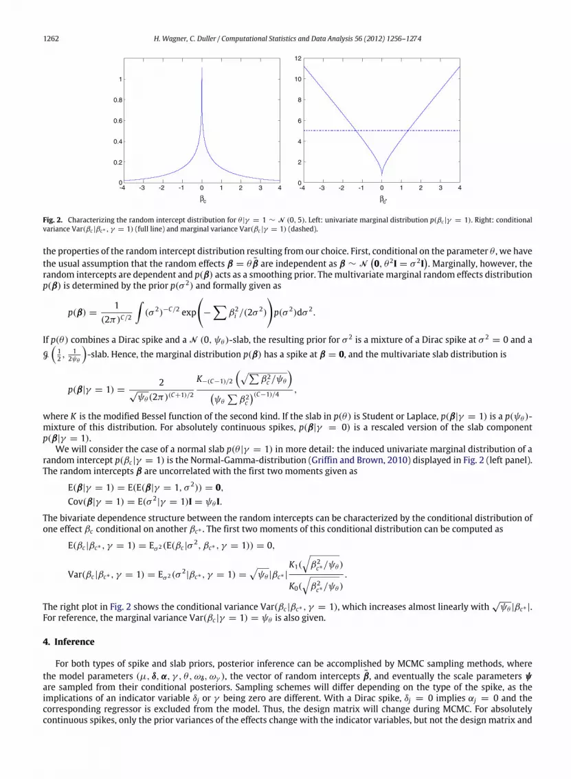
Fig. 2. Characterizing the random intercept distribution for θ |γ = 1 ∼ N (0, 5). Left: univariate marginal distribution p(βc |γ = 1). Right: conditionalvariance Var(βc |βc∗ , γ = 1) (full line) and marginal variance Var(βc |γ = 1) (dashed).

the properties of the random intercept distribution resulting from our choice. First, conditional on the parameter θ , we havethe usual assumption that the random effects β = θ β are independent as β ∼ N

0, θ2I = σ 2I

. Marginally, however, the

random intercepts are dependent and p(β) acts as a smoothing prior. Themultivariate marginal random effects distributionp(β) is determined by the prior p(σ 2) and formally given as

p(β) =1

(2π)C/2

(σ 2)−C/2 exp

−

β2i /(2σ

2)

p(σ 2)dσ 2.

If p(θ) combines a Dirac spike and a N (0, ψθ )-slab, the resulting prior for σ 2 is a mixture of a Dirac spike at σ 2= 0 and a

G

12 ,

12ψθ

-slab. Hence, the marginal distribution p(β) has a spike at β = 0, and the multivariate slab distribution is

p(β|γ = 1) =2

√ψθ (2π)(C+1)/2

K−(C−1)/2

β2c /ψθ

ψθβ2c

(C−1)/4 ,

where K is the modified Bessel function of the second kind. If the slab in p(θ) is Student or Laplace, p(β|γ = 1) is a p(ψθ )-mixture of this distribution. For absolutely continuous spikes, p(β|γ = 0) is a rescaled version of the slab componentp(β|γ = 1).

We will consider the case of a normal slab p(θ |γ = 1) in more detail: the induced univariate marginal distribution of arandom intercept p(βc |γ = 1) is the Normal-Gamma-distribution (Griffin and Brown, 2010) displayed in Fig. 2 (left panel).The random intercepts β are uncorrelated with the first two moments given as

E(β|γ = 1) = E(E(β|γ = 1, σ 2)) = 0,Cov(β|γ = 1) = E(σ 2

|γ = 1)I = ψθ I.

The bivariate dependence structure between the random intercepts can be characterized by the conditional distribution ofone effect βc conditional on another βc∗ . The first two moments of this conditional distribution can be computed as

E(βc |βc∗ , γ = 1) = Eσ 2(E(βc |σ2, βc∗ , γ = 1)) = 0,

Var(βc |βc∗ , γ = 1) = Eσ 2(σ 2|βc∗ , γ = 1) =

ψθ |βc∗ |

K1(

β2c∗/ψθ )

K0(

β2c∗/ψθ )

.

The right plot in Fig. 2 shows the conditional variance Var(βc |βc∗ , γ = 1), which increases almost linearly with√ψθ |βc∗ |.

For reference, the marginal variance Var(βc |γ = 1) = ψθ is also given.

4. Inference

For both types of spike and slab priors, posterior inference can be accomplished by MCMC sampling methods, wherethe model parameters (µ, δ,α, γ , θ, ωδ, ωγ ), the vector of random intercepts β, and eventually the scale parameters ψare sampled from their conditional posteriors. Sampling schemes will differ depending on the type of the spike, as theimplications of an indicator variable δj or γ being zero are different. With a Dirac spike, δj = 0 implies αj = 0 and thecorresponding regressor is excluded from the model. Thus, the design matrix will change during MCMC. For absolutelycontinuous spikes, only the prior variances of the effects change with the indicator variables, but not the design matrix and


therefore the model dimension is fixed. As the value of the indicator δj does not determine the value of the correspondingeffect αj and vice versa, δj can be sampled conditionally on αj. In contrast, for a Dirac spike, sampling δj conditional onthe effect αj is not possible: as δj = 0 ↔ αj = 0, MCMC could get stuck at αj = 0, resulting in a reducible, non-convergent Markov chain (George and McCulloch, 1997). Therefore, when a Dirac spike is used, it is essential to draw theindicator variables (δ, γ ) from the marginal likelihood p(δ, γ |y) integrating over the parameters subject to selection, seeGeweke (1996) and Smith and Kohn (1996). This requires evaluation of marginal likelihoods in each iteration, which iscomputationally demanding except for normal regression models under conjugate priors. Therefore, we make use of dataaugmentation, as in Frühwirth-Schnatter and Frühwirth (2010) to achieve a representation of the logit model as a normalregression model. Data augmentation for logit models is outlined first in Section 4.1, and then the sampling scheme formodel selection in the study model is presented in Section 4.2.

4.1. Data augmentation for binary logit type models

The logit random intercept model can be specified using a latent variableui = µ+ xiα+ βc(i) + εi,

where the error term εi follows a standard logistic distribution εi ∼ Log(0, 1) and the latent variable is related to theresponse by

yi = I{ui > 0}.As shown in Monahan and Stefanski (1992), the standard logistic density can be approximated very accurately by a scalemixture of only six normal components with mean 0,

f (ε) =eε

(1 + eε)2≈ g(ε) =

6r=1

wr fN(ε; 0, s2r ),

see also Frühwirth-Schnatter and Frühwirth (2010). Data augmentation, where the latent variables u = (u1, . . . , un) andthe indicators r = (r1, . . . , rn) of the normal mixture components are introduced, allows a representation of the selectionmodel defined by Eq. (6) as

ui = µ+

dj=1

xijαj + βc(i)θ + εri , εri ∼ N0, s2ri

, (7)

βc(i) ∼ N (0, 1) , (8)with the priors specified in Section 3.4.

4.2. MCMC sampling scheme

Based on the auxiliary mixture representation (7), MCMC for sampling the model parameters from their posteriordistribution involves the following steps:(1) Sample u and r conditional on µ,α, and β as summarized in Appendix A.(2) Sample ωδ and ωγ independently from their posteriors ωδ ∼ B

aδ,0 + d1, bδ,0 + d − d1

, where d1 =

δj and

ωγ ∼ Baγ ,0 + γ , bγ ,0 + 1 − γ

.

(3) Sample the indicators (δ, γ ), the parameters (µ,α, θ), and if required, the scale parameters ψ. Details of this samplingstep, which depends on the type of spike, are given in Section 4.2.1 for absolutely continuous and in Section 4.2.2 forDirac spikes.

(4) Sample the random effects β conditional on (µ,α, θ, r,u) from the model

y = u − µ− Xα = θHβ + ε, ε ∼ N (0,6) ,where H is a matrix which selects the appropriate random intercept for each observation and 6 = diag(s2r1 , . . . , s

2rn).

The conditional posterior p(β|θ,6, y) is a normal distribution N (b, B)with moments given as

B−1= θ2 · H′6−1H + I,

b = θ · BH′6−1y.(5) To explore the whole range of the posterior, perform a random sign-switch for θ and β, where the sign of θ and all

random effects is changed with probability 0.5. By construction, θ = ±√σ 2 has a symmetric posterior distribution

which will be bimodal for σ 2 > 0. The random sign-switch step guarantees that the full, eventually bimodal, posteriordistribution is explored in a balanced way.

4.2.1. Sampling steps for an absolutely continuous spikeFor absolutely continuous spikes, it is possible to sample (δ, γ ) andψ together in one block as the full conditional of the

parameters (δ, γ ,ψ) has the structure


p(δ, γ ,ψ|α, θ, ωδ, ωγ , y) =

dj=1

p(ψj|δj, αj)p(δj|αj, ωδ)p(ψθ |γ , θ)p(γ |θ, ωγ ).

Sampling step (3) is therefore implemented as follows:

(3a) Sample (δ, γ ,ψ).(i) For j = 1, . . . , d, sample δj from

p(δj = 1|αj, ωδ) =1

1 +1−ωδωδ

Lj, Lj =

pspike(αj)

pslab(αj),

and sample γ from

p(γ = 1|θ, ωγ ) =1

1 +1−ωγωγ

L, L =

pspike(θ)pslab(θ)

.

(ii) For normal spikes and slabs, set ψj ≡ V and ψθ ≡ V . Otherwise, sample ψj, j = 1, . . . , d from the posteriorp(ψj|αj, δj) and sample ψθ from p(ψθ |θ, γ ).The form of the posterior p(ψj|αj, δj) depends on the prior p(ψj): For ψj ∼ G−1 (ν,Q ), the posterior is given as

ψj|δj, αj ∼ G−1 ν + 1/2,Q + α2j /(2r(δj))

,

and for the exponential prior ψj ∼ E (1/2λ), the posterior is a generalized inverse Gaussian distributionψj|αj, δj ∼ GIG

1/2, 1/λ, α2

j /r(δj).

Modifications for sampling ψθ are straightforward.(3b) Sample ζ = (µ,α, θ) in one block from the normal posterior N (an,An) of the regression model

u = Zζ + ε, ε ∼ N (0,6) ,

with design matrix Z = [1,X, β], error covariance matrix 6 = diag(s2r1 , . . . , s2rn), and prior ζ ∼ N (0,A0). Here, A0

is a diagonal matrix with entriesM0, r(δ1)ψ1, . . . , r(δd)ψd, r(γ )ψθ

. Alternatively, ζ could be drawn omitting the

data augmentation step (1) directly from the posterior p(ζ|δ, γ , β,ψ, y), e.g. by a Metropolis Hastings step using aniteratively weighted least squares proposal as in Brezger and Lang (2006). However, as shown in Frühwirth-Schnatterand Frühwirth (2010), auxiliary mixture sampling is fast and efficient compared to other sampling methods for logittype models.

4.2.2. Sampling steps for a Dirac spikeTo avoid reducibility of the resulting Markov chain, integration over the effects subject to selection is essential when a

prior with Dirac spike is used. Therefore, implementation of sampling step (3) differs compared to that for an absolutelycontinuous spike. In contrast to Section 4.2.1, where (δ, γ ) and the scale parameters ψ are drawn in one block, for a Diracspike, a different blocking scheme is used where (δ, γ ) and ζ are sampled together.

(3a) Sample (δ, γ , ζ) from the posterior p(δ, γ , ζ|u, ωδ, ωγ ,ϒ)whereϒ = (r, β,ψ).(i) Sample each element δj of the indicator vector δ separately from p(δj|δ\j, γ ,u, ωδ, ωγ ,ϒ), where δ\j denotes the

vector δ consisting of all elements of δ except δj. Sample γ from the conditional posterior p(γ |δ,u, ωδ, ωγ ,ϒ).Elements of δ are updated in a random permutation order. Further details of this step are given below.

(ii) Set αj = 0 if δj = 0 and θ = 0 if γ = 0. Sample the vector ζ∗ consisting of µ, the non-zero elements αδ, and θ , ifγ = 1 from the regression model

u = Z∗ζ∗+ ε, ε ∼ N (0,6) ,

with design matrix Z∗= [1,Xδ, β] if γ = 1, and Z∗

= [1,Xδ] otherwise. Here Xδ denotes the design matrix ofthe restricted model, including only those columns of X where the corresponding indicator δj = 1. The prior forζ∗ is the normal distribution, N (0,A0), where A0 is a diagonal matrix with entriesM0, the scale parametersψj foreffects where δj = 1 and ψθ , if γ = 1.

(3b) For j = 1, . . . , d, sample ψj from the posterior p(ψj|δj, αj) and sample ψθ from the posterior p(ψθ |γ , θ). For δj = 0,the prior of ψj is independent of αj (see Eq. (4)), and therefore, the conditional posterior, given as

p(ψj|δj, αj) = p(ψj),

is equal to the prior distribution. For δj = 1, sampling is performed as described in step (3a)(ii) of Section 4.2.1. Thesame applies to ψθ .

We describe sampling step (3a) in detail. The conditional posterior of δj, given as

p(δj = 1|δ\j, γ ,u, ωδ, ωγ ,ϒ) ∝ p(u|δj = 1, δ\j, γ ,ϒ)ωδ,

can be computed from

p(δj = 1|δ\j, γ ,u, ωδ, ωγ ,ϒ) =1

1 +1−ωδωδ

Kj, Kj =

p(u|δj = 0, δ\j, γ ,ϒ)p(u|δj = 1, δ\j, γ ,ϒ)

.


It involves the conditional marginal likelihoods of two heteroscedastic linear regression models with design matricesdiffering only by inclusion/exclusion of regressor xj. The conditional marginal likelihood of a linear regression model isavailable in closed form as

p(u|δ, γ ,ϒ) =1

(2π)n/2|An|

1/2

|A0|1/2

exp−1/2(u′6−1u − a′

nA−1n an + a′

0A−10 a0)

,

where an and An are the moments of the normal posterior

An = ((Z∗)′6−1Z∗+ A−1

0 )−1, an = An(Z∗)′6−1u + A−1

0 a0,and Z∗ is the appropriate designmatrix, including those regressors, for which the corresponding indicator variable takes thevalue 1. Analogously, the conditional posterior of γ is given as

p(γ = 1|δ,u, ωδ, ωγ ,ϒ) =1

1 +1−ωγωγ

K, K =

p(u|γ = 0, δ,ϒ)p(u|γ = 1, δ,ϒ)

,

and requires the conditional marginal likelihoods of two regression models differing only by inclusion/exclusion of β in thedesign matrix Z∗.

4.3. Estimation of posterior inclusion probabilities

In both sampling schemes, conditional posterior inclusion probabilities p(δj = 1|y,∼) and p(γ = 1|y,∼) are computedin each MCMC iteration m = 1, . . . ,M in sampling step (3a)(i). We denote these values by p(m)(δj = 1|y,∼) andp(m)(γ = 1|y,∼). Storing these conditional posterior inclusion probabilities allows to estimate p(δj|y) by the mean

pj = p(δj = 1|y) =1M

Mm=1

p(m)(δj = 1|y,∼),

and p(γ = 1|y) by the mean of p(m)(γ = 1|y,∼), m = 1, . . . ,M , which we will denote by pγ . As MCMC drawsare autocorrelated, sampling efficiency of different sampling schemes can be compared by the effective sample size ESS,which estimates the number of independent samples required to obtain a parameter estimate with the same precisionas the MCMC estimate. It is computed as ESS = M/τ , where the τ is the integrated autocorrelation time (IAT), definedas τ = 1 + 2

Ll=1 ρ(l) and ρ(l) is the empirical autocorrelation at lag l. To determine L, the initial monotone sequence

estimator (Geyer, 1992) can be used.Marginalization usually leads to less autocorrelated draws, and therefore, integrated autocorrelation times can be

expected to be smaller using the sampling scheme for Dirac spikes. As remarked above, absolutely continuous spikes havethe advantage that indicator variables can be drawn conditional on the corresponding effects, as 0 < p(δj = 1|αj) < 1for r > 0 and ψj < ∞. As seen from Fig. 1, the conditional prior inclusion probabilities p(δj = 1|αj) are close to zero andone for a wide range of αj, in particular for the normal spike and slab prior. The gradient is smaller for heavy-tailed spikes,which should encourage moves between the spike and the slab component and hence, produce less autocorrelated drawsp(m)(δj = 1|y,∼) and p(m)(γ = 1|y,∼).

5. Simulated data

In this section, we investigate the performance of the MCMC implementations under different spike and slab priors forsimulated data. The first simulation study deals with a relatively simple data situation with 10 potential covariates, bothwith andwithout random intercept. In the second simulation study, we use the designmatrix of the ERCP data togetherwiththe estimated effects in the finally selected model to generate artificial data. In both simulation studies the uninformativeB (1, 1)-prior was used for ωδ and ωγ . As variances of the slab distributions are matched, only values for the variance ofthe normal slab V , the degrees of freedom for the Student components ν and the variance ratio r for priors with absolutelycontinuous spikes have to be chosen. Following Fahrmeir et al. (2010), we used V = 5 and ν = 5, and thus, the resultingStudent components have 2ν = 10 degrees of freedom, guaranteeing the existence of posterior moments of order smallerthan 10 even in a separation case. The hyper-parameters Q and λ are Q = V (ν − 1) = 20 and λ = V/2 = 2.5, for detailssee Section 3.3.1. Further, as in Fahrmeir et al. (2010) the variance ratio r was set to r = 0.0052, but we investigate differentchoices in the first simulation study. MCMC schemes were implemented in Matlab functions written by the first author.Draws from the GIG-Distribution were obtained from the ‘randraw’ toolbox, available from Matlab Download Central. Allcomputations were run on a Intel Core i7, 1.6 GHz laptop.

5.1. Simulation study 1

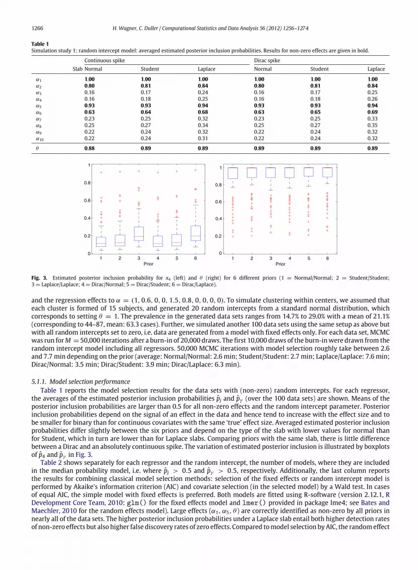
We generated 100 data sets with n = 300 simulated responses from a logit model with random intercepts. d = 10regressors were generated, four of them continuous N (0, 1)-variables and six binary with p(xi) = 0.5. We set µ = −2


Table 1Simulation study 1; random intercept model: averaged estimated posterior inclusion probabilities. Results for non-zero effects are given in bold.

Continuous spike Dirac spikeSlab Normal Student Laplace Normal Student Laplace

α1 1.00 1.00 1.00 1.00 1.00 1.00α2 0.80 0.81 0.84 0.80 0.81 0.84α3 0.16 0.17 0.24 0.16 0.17 0.25α4 0.16 0.18 0.25 0.16 0.18 0.26α5 0.93 0.93 0.94 0.93 0.93 0.94α6 0.63 0.64 0.68 0.63 0.65 0.69α7 0.23 0.25 0.32 0.23 0.25 0.33α8 0.25 0.27 0.34 0.25 0.27 0.35α9 0.22 0.24 0.32 0.22 0.24 0.32α10 0.22 0.24 0.31 0.22 0.24 0.32

θ 0.88 0.89 0.89 0.89 0.89 0.89

0 0

0.2 0.2

0.4 0.4

0.6 0.6

0.8 0.8

11

1 2 3 4 5 6Prior

1 2 3 4 5 6Prior

Fig. 3. Estimated posterior inclusion probability for x4 (left) and θ (right) for 6 different priors (1 = Normal/Normal; 2 = Student/Student;3 = Laplace/Laplace; 4 = Dirac/Normal; 5 = Dirac/Student; 6 = Dirac/Laplace).

and the regression effects to α = (1, 0.6, 0, 0, 1.5, 0.8, 0, 0, 0, 0). To simulate clustering within centers, we assumed thateach cluster is formed of 15 subjects, and generated 20 random intercepts from a standard normal distribution, whichcorresponds to setting θ = 1. The prevalence in the generated data sets ranges from 14.7% to 29.0% with a mean of 21.1%(corresponding to 44–87, mean: 63.3 cases). Further, we simulated another 100 data sets using the same setup as above butwith all random intercepts set to zero, i.e. data are generated from a model with fixed effects only. For each data set, MCMCwas run forM = 50,000 iterations after a burn-in of 20,000 draws. The first 10,000 draws of the burn-inwere drawn from therandom intercept model including all regressors. 50,000 MCMC iterations with model selection roughly take between 2.6and 7.7min depending on the prior (average: Normal/Normal: 2.6min; Student/Student: 2.7min; Laplace/Laplace: 7.6min;Dirac/Normal: 3.5 min; Dirac/Student: 3.9 min; Dirac/Laplace: 6.3 min).

5.1.1. Model selection performanceTable 1 reports the model selection results for the data sets with (non-zero) random intercepts. For each regressor,

the averages of the estimated posterior inclusion probabilities pj and pγ (over the 100 data sets) are shown. Means of theposterior inclusion probabilities are larger than 0.5 for all non-zero effects and the random intercept parameter. Posteriorinclusion probabilities depend on the signal of an effect in the data and hence tend to increase with the effect size and tobe smaller for binary than for continuous covariates with the same ‘true’ effect size. Averaged estimated posterior inclusionprobabilities differ slightly between the six priors and depend on the type of the slab with lower values for normal thanfor Student, which in turn are lower than for Laplace slabs. Comparing priors with the same slab, there is little differencebetween a Dirac and an absolutely continuous spike. The variation of estimated posterior inclusion is illustrated by boxplotsof p4 and pγ in Fig. 3.

Table 2 shows separately for each regressor and the random intercept, the number of models, where they are includedin the median probability model, i.e. where pj > 0.5 and pγ > 0.5, respectively. Additionally, the last column reportsthe results for combining classical model selection methods: selection of the fixed effects or random intercept model isperformed by Akaike’s information criterion (AIC) and covariate selection (in the selected model) by a Wald test. In casesof equal AIC, the simple model with fixed effects is preferred. Both models are fitted using R-software (version 2.12.1, RDevelopment Core Team, 2010: glm() for the fixed effects model and lmer() provided in package lme4; see Bates andMaechler, 2010 for the random effects model). Large effects (α1, α5, θ ) are correctly identified as non-zero by all priors innearly all of the data sets. The higher posterior inclusion probabilities under a Laplace slab entail both higher detection ratesof non-zero effects but also higher false discovery rates of zero effects. Compared tomodel selection byAIC, the randomeffect


Table 2Simulation study 1; random intercept model: number of models where a regressor is selected in themedian probability model. Results for non-zero effectsare given in bold.

Continuous spike Dirac spike AICSlab Normal Student Laplace Normal Student Laplace Wald test

α1 100 100 100 100 100 100 100α2 84 84 87 84 84 89 92α3 5 6 9 5 6 9 6α4 4 4 9 4 4 10 8α5 95 95 96 95 95 96 95α6 61 63 70 61 66 72 65α7 5 8 10 7 8 12 3α8 8 10 15 7 11 16 10α9 6 6 10 5 7 11 3α10 3 5 9 3 5 11 3

θ 93 94 93 93 93 95 87

Table 3Simulation study 1; fixed effects model: averaged estimated posterior inclusion probabilities. Results for non-zero effects are given in bold.


α1 1.00 1.00 1.00 1.00 1.00 1.00α2 0.80 0.81 0.83 0.80 0.81 0.84α3 0.15 0.16 0.23 0.15 0.16 0.24α4 0.15 0.17 0.24 0.15 0.17 0.24α5 0.97 0.97 0.97 0.97 0.97 0.98α6 0.62 0.63 0.67 0.62 0.63 0.67α7 0.22 0.24 0.31 0.22 0.24 0.32α8 0.23 0.25 0.33 0.23 0.25 0.33α9 0.22 0.24 0.32 0.22 0.24 0.32α10 0.22 0.23 0.31 0.22 0.24 0.32

θ 0.24 0.25 0.29 0.24 0.25 0.29

Table 4Simulation study 1; fixed effects model: number of models where a regressor is selected in the median probability model. Results for non-zero effects aregiven in bold.

Continuous spike Dirac spike AICSlab Normal Student Laplace Normal Student Laplace Wald test

α1 100 100 100 100 100 100 100α2 82 82 87 82 83 88 89α3 3 3 5 3 3 5 4α4 2 3 4 2 2 4 5α5 99 99 99 99 99 100 99α6 60 63 66 60 61 70 61α7 5 6 8 5 6 8 3α8 8 8 11 8 8 11 6α9 7 7 8 7 7 10 5α10 6 7 10 4 7 10 2

θ 8 9 10 9 9 10 5

is detected as non-zeromore often under all priors. Variable selection by aWald test in the selectedmodel performs roughlysimilar as the Bayesian model selection method. For the data sets generated from the fixed effects model, the averages ofestimated posterior inclusion probabilities (see Table 3) for all covariates are almost identical to the results for the datagenerated from the random intercept model. Further, the number of data sets where a regressor is selected in the medianprobability model is roughly equal, see Table 4. The percentage of data sets where a random intercept is selected rangesfrom 8% up to 10%, depending on the prior.

5.1.2. Comparing efficienciesIntegrated autocorrelation times (IAT), and hence ESSs cannot be computed in clear-cut situations, where allM draws of

a posterior inclusion probability p(m)(δj|y,∼) or p(m)(γ |y,∼) are either equal to zero or one. Therefore, theywere computedonly if the posterior inclusion probability was numerically different from 1 in at least one draw. Tables 5 and 6 report the


Table 5Simulation study 1; random intercept model: median integrated autocorrelation times of the posterior inclusion probabilities.


α1 1.0∗ 1.1 1.0∗ 1.2∗ 1.1∗ 1.2∗

α2 142.1∗ 118.7 76.0 13.5 13.0 11.4α3 22.3 19.6 18.3 6.3 6.5 6.2α4 20.4 19.8 17.7 6.0 6.1 6.1α5 169.9∗ 39.1 68.4∗ 5.9 6.0 5.3α6 125.6∗ 104.9 71.0 13.2 12.4 10.6α7 31.2 28.7 24.5 6.2 6.3 6.3α8 36.3 32.9 27.3 6.9 7.4 6.8α9 33.8 29.8 25.2 6.7 6.4 6.3α10 31.3 28.7 24.8 6.5 6.3 6.2

θ 187.6∗ 114.0 104.8∗ 40.7 44.3 34.0

Table 6Simulation study 1; random intercept model: median effective sample size per sec. of the posterior inclusion probabilities.


α1 319.5∗ 287.2 107.6∗ 196.6∗ 199.2∗ 121.2∗

α2 2.3∗ 2.7 1.4 18.3 18.1 14.2α3 14.6 16.3 5.8 37.7 36.3 23.9α4 16.1 16.0 6.1 40.3 37.6 23.5α5 1.9∗ 8.2 1.6∗ 38.3 39.9 28.5α6 2.6∗ 3.0 1.5 18.4 18.6 14.2α7 10.4 10.9 4.4 37.0 35.3 23.3α8 8.9 9.5 4.0 33.9 32.6 21.7α9 9.7 10.7 4.3 36.6 33.7 22.5α10 10.5 11.1 4.4 37.1 36.5 24.8

θ 1.7∗ 2.8 1.0∗ 6.1 5.3 4.6

median IAT and the median ESS per second (ESS/s.) for each posterior inclusion probability in the relevant data sets. Resultsmarked with a star are based on less than all 100 data sets: for Dirac spikes, results for p(δ1 = 1|y) are based on 98 datasets, for absolutely continuous spikes, the numbers of relevant data sets are given in Table 7, which compares the resultsfor different variance ratios r . As expected, IATs are higher for absolutely continuous than for Dirac spikes. The valuesare similar for all priors with Dirac spikes and smallest for the Dirac/Laplace prior. Priors with heavy-tailed spikes andslabs, i.e. Laplace and Student, yield better mixing MCMC chains than the normal/normal prior. Further, IATs are smaller foreffects with estimated posterior inclusion probability closer to the boundaries 0 and 1 and are highest for α2 and α6. Withregard to ESS per second (computed as ESS divided by total computation time for the draws after burn-in), MCMC for theDirac/Normal and Dirac/Student priors outperform the other settings. The computational costs of marginalization (whichrequires inversion and computing the determinant of the matrix An) are higher than drawing indicators conditional on theeffect, yet not high enough to be outweighed by the higher IATs for absolutely continuous spikes. Drawing from the GIG-distribution is particularly costly and the advantage of less autocorrelated draws for Laplace slabs is lost when computationtime is taken into account.

5.1.3. Effect of the variance ratioTo assess the sensitivity of the results with regard to the variance ratio r , we repeated the analysis (for the simulated

data with random intercept) using priors with absolutely continuous spikes with r = 0.012 and r = 0.0012. Averagedinclusion probabilities and number of data sets where a regressor is selected are almost identical when comparing the sameslab distribution under different values of the variance ratio r . Table 7 reports the median IATs in data sets where at leastone draw of the posterior inclusion probabilities was numerically different from 1. If different from 100, the number of datasets on which the median is based is given in parentheses as a superscript. Though in principle possible, we never observedMCMC getting stuck at posterior inclusion probabilities of 0.

TomimicDirac spikes closely, small variance ratios r would be preferred. However, as seen fromTable 7, IATs and numberof data sets where MCMC chains get stuck at conditional posterior inclusion probabilities of 1 decrease with the varianceratio r . Basically, there are two different situations where inclusion probabilities could equal 1 in each MCMC iteration: thecase where evidence for inclusion of an effect is overwhelming and the case where MCMC gets stuck though the posteriorinclusion probability is smaller than 1. Though exact posterior inclusion probabilities are not available, from the results ofour previous analysis we suspect that the latter is the case for α2 and α6 under a normal/normal prior and a Laplace/Laplaceprior. As a result, we conclude that MCMC mixes reasonably well for the Student/Student prior with r ≥ 0.0052 and theLaplace/Laplace prior with r = 0.012.


Table 7Simulation study 1: comparing median IATs of inclusion probabilities for different variance ratios.

Slab Normal Student Laplacer 0.0012 0.0052 0.012 0.0012 0.0052 0.012 0.0012 0.052 0.012

α1 1.0(13) 1.0(28) 1.0(48) 1.0(75) 1.1 1.4 1.0(22) 1.0(77) 1.0(99)

α2 439.4(75) 142.1(93) 91.5 266.0 118.7 68.9 219.7(90) 76.0 47.5α3 69.2 22.3 13.6 65.9 19.6 13.8 53.3 18.3 13.4α4 74.6 20.4 13.5 61.9 19.8 14.0 52.0 17.7 13.0α5 437.4(50) 169.9(59) 83.1(70) 167.7(81) 39.1 36.5 238.8(61) 68.4(84) 35.3(98)

α6 407.2(95) 125.6(98) 75.1(99) 311.3 104.9 68.8 204.4(99) 71.0 47.4α7 124.1 31.2 18.4 100.8 28.7 18.6 80.6 24.5 15.6α8 130.4 36.3 22.8 106.4 32.9 21.4 82.4 27.3 18.4α9 125.8 33.8 20.5 105.1 29.8 18.7 81.6 25.2 16.3α10 125.7 31.3 19.4 100.0 28.7 18.2 80.1 24.8 15.6

θ 458.5(59) 187.6(67) 127.5(75) 223.6(84) 114.0 78.9 237.7(70) 104.8(90) 78.1

Table 8Simulation study 2: variables leading to separation.

Variable 4 5 6 11 18 21 27 34Number of data sets 5 1 1 2 5 2 6 8

Table 9Simulation study 2: number of data sets where a regressor is selected in the median probability model. Results for true non-zero effects are given in bold.

Continuous spike Dirac spike PML AICSlab Normal Student Laplace Normal Student Laplace Wald test

α5 0 1 0 0 0 0 3 3α10 1 1 1 1 1 1 1 1α12 4 4 4 4 4 4 3 3α13 3 3 3 3 3 3 2 2α21 10 10 10 10 10 10 10 7α25 9 9 9 9 9 9 10 10α29 2 3 2 2 2 3 2 2α31 7 7 7 7 7 7 3 1α32 2 2 2 2 2 2 1 1α34 8 8 8 8 8 8 4 0

θ 0 0 0 0 0 0 – 0

5.2. Simulation study 2

In our second simulation study, we generated 10 data sets with the design matrix of the ERCP data and the parametervalues µ = −4.27 and (α12, α13, α21, α25, α31, α34) = (0.5, 0.5, 3.2, 1.0,−1.7,−2.6). The remaining 31 elements of αand the random intercept parameter were set to zero. This data generating process corresponds to the estimated parametervalues of the finally selectedmodel for the ERCP data, see Section 6.2. The prevalence in the generated data sets ranges from3.34% to 3.85% with a mean of 3.64% (Number of events: 105–121; mean: 121). Separation occurs in all but one data set.Table 8 reports the number of data sets where a specific covariate separates cases and non-cases. Variables not mentioneddid not lead to separation in any of the 10 data sets.

MCMCwas run for 700,000 iterations for absolutely continuous and 300,000 iterations for Dirac spikes after a burn-in of100,000. The first 10,000 draws of the burn-in were drawn from the unrestricted model.

5.2.1. Model selection resultsTable 9 reports the number of data sets for which each regressor and the random effect, respectively is selected in the

median probabilitymodel. Regressors not listed in this table are selected in none of the data sets under any of the six differentpriors. Again, the results for the different priors conform well. The center-specific random intercept was never selected.Additionally results of classical selection procedures are reported. Column AIC/Wald test again reports the model selectionresults based on AIC combined with a Wald test. The additional column PML gives the results for the penalized ML methodrecommended by Heinze (2006) for logistic regression with separated or nearly separated data. AIC chooses a fixed effectsmodel in all data sets; PML inference is not implemented for random intercept models, and hence, the results only refer tocovariate selection. Both methods also select effects not mentioned in Table 9 in one (PML: α3, α4, α13, α17, α22, α23, α30;Wald test: α4, α14, α17, α22) or two data sets (PML: α2, α7, α16, α24, α29, α36; Wald test: α2, α3, α7, α16, α23, α24, α30, α36).This simulation study clearly shows the advantages of the Bayesian model selection procedure: it performs model selection


0

0

1

2

3

4

5

6

100

200

300

400

500

1 2 3 4 5 6Prior

1 2 3 4 5 6Prior

Fig. 4. IAT (left) and ESS/s. (right) of the posterior inclusion probabilities of regression effects under six different prior distributions (1 = Normal/Normal;2 = Student/Student; 3 = Laplace/Laplace; 4 = Dirac/Normal; 5 = Dirac/Student; 6 = Dirac/Laplace).

with regard to inclusion of regressors aswell as the center-specific random intercept at the same time, can handle separationand performs better in discriminating zero and non-zero effects.

5.2.2. Sampling efficiencySampling efficiency of posterior inclusion probabilities show large variation depending on the type of the prior and the

strength of the effect signal in the data. To give an overall picture, Fig. 4 shows IATs and ESSs per sec. under the different priorsin a boxplot for all regression effects (except α21) in the 10 data sets, i.e. a box (plus whiskers and outliers) corresponds to360 effects for each prior. IATs larger than 500 occur only for absolutely continuous spikes and are not shown in the plot. Themaximum IAT is 1191.0 for the normal/normal prior, 865.4 for the Student/Student prior, and 529.8 for the Laplace/Laplaceprior.

Confirming with simulation study 1, IATs are higher for priors with absolutely continuous spikes than for their counter-parts with Dirac spikes. Priors with heavy-tailed spikes and slabs perform better than the Normal/Normal distribution. Thedifferences in IATs between Dirac and absolutely continuous spikes are smaller for the posterior inclusion probability of therandom intercept parameter θ than for the regression effects. Again, IATs are higher for medium posterior inclusion proba-bilities. As computational costs increase linearly with the dimension of the design matrix for absolutely continuous spikesbut more than linearly for Dirac spikes, in this higher-dimensional setting, higher IATs for absolutely continuous spikes areoutweighed by smaller computing time. With regard to the median ESS/s. the Student/Student prior slightly outperformsthe other priors.

6. Application

To identify potential risk factors for bleeding after ERCP, we used the data of patients experiencing ERCP for their firsttime only from those 27 centers reporting at least 5 ERCPs, leaving data on 3143 patients for the analysis. The resultingcluster sizes have high variation, ranging from 5 to 453 cases in one clinic. Risk of bleeding is small and was observed for118 or 3.8% of the patients. As potential risk factors we used age and 36 binary covariates indicating the presence/absence ofa risk factor. As mentioned above, some of the risk factors are rare and separation occurred for three covariates (indicationpancreatic duct stones, controlling pulse oximetry, and previous gastric surgery).

6.1. Exploratory Bayesian analysis

As a first step, we performed a Bayes analysis of the unrestricted model in the non-centered parameterization using anormal prior with zero mean and variance V = 5. Fig. 5 shows the posterior estimates and 95%-credible intervals of theregression effects and the random intercepts. These intervals contain zero for most of the covariates and for all randomintercepts, which suggests that a restricted model without random intercept might be appropriate for the data. In Fig. 6, theposterior distribution of θ is compared to its prior distribution. The estimated Savage–Dickey density ratio with a value ofpθ (0|y)pθ (0)

= 1.3 also slightly supports a model without random intercept.

6.2. Model selection

Model selection for the non-centered logit random intercept model was performed under six different spike and slabpriors with hyper-parameters chosen as in the simulation studies, i.e. V = 5, ν = 5, and r = 0.0052. The choice of theparameters V and r can be based on properties of priors with absolutely continuous spikes: as discussed in Section 3.3.1with these values for V and r , the prior inclusion probability of an effect leading to an increase or decrease of the risk by


–6

–4

–2

–2

–1.5

–1

–0.5

0

0.5

1

1.5

2

0

2

4

6

0 0 5 10 15 20 255 10 15 20 25 30 35

Covariate number Clinic number

Fig. 5. Posterior means and 95%-credible intervals for regression effects (left) and random intercepts (right).

0

0.1

0.2

0.3

0.4

0.5

0.6

0.7

0.8

0.9

–2 –1.5 –0.5–1 0 1 21.50.5

posteriorprior

Fig. 6. Kernel density estimate of the posterior distribution of θ .

Table 10ERCP data: estimated posterior inclusion probabilities for selected covariates.

Nr. Covariate Continuous spike Dirac spikeSlab Normal Student Laplace Normal Student Laplace

12 Severe disease 0.54 0.50 0.58 0.59 0.58 0.6213 Anticoagulation 0.46 0.53 0.56 0.50 0.53 0.5721 Sphincterotomy 1.00 1.00 1.00 1.00 1.00 1.0025 Other intervention 1.00 1.00 1.00 1.00 1.00 1.0031 Vis. of the relevant duct 0.73 0.72 0.72 0.72 0.73 0.7234 Previous gastric surgery 0.61 0.60 0.61 0.62 0.61 0.59

roughly 4% (corresponding to 16 events for 10,000 procedures), will be at least 0.5. MCMC was run for 700,000 iterationsfor absolutely continuous and 300,000 iterations for Dirac spikes after a burn-in of 100,000. The first 10,000 draws ofthe burn-in were drawn from the unrestricted model. Convergence was checked by starting MCMC from the null model(including only the intercept) under each prior yielding essentially the same results. 100,000 MCMC iterations took about21 min for Normal/Normal and Student/Student priors and roughly an hour for the other priors (Laplace/Laplace: 55 min;Dirac/Normal: 62 min; Dirac/Student: 63 min; Dirac/Laplace: 76.5 min).

Posterior inclusion probabilities were rather similar for all covariates under all priors. Based on a posterior inclusionprobability larger than 0.5, the selected covariates are severe disease, sphincterotomy, other intervention, visualization ofthe relevant duct, and previous gastric surgery. All priorswith the exception of the normal/normal prior additionally selectedanticoagulation as a further risk factor for bleeding after ERCP. The estimatedposterior inclusionprobabilities for the selectedcovariates are shown in Table 10. These results are in line with the results in literature, in so far as sphincterotomy andother inventions were selected, but other factors such as age, gender, experience of endoscopist, and size of center werenot. Results for random intercept selection are shown in Table 11. With a cut-off point of 0.5 for the estimated posteriorinclusion probabilities, the selected model therefore is a fixed effects model with the six covariates listed in Table 10.

To give more detailed insight in MCMC performance, Table 12 reports the maximum IATs and the minimum ESS/s. forpj categorized in three classes (smaller than 0.1; between 0.1 and 0.4; between 0.4 and 0.99). Maximum IAT and minimumESS/s. are reported as these correspond to the worst case in each category. Under all priors, sampling efficiency is lowestfor the posterior inclusion probabilities of either covariate 12, 13, or 34, i.e. for those covariates with estimated posteriorinclusion probability not too far from 0.5. Comparing the results under different priors, again (as in simulation study 2) thereis a slight preference for the Student/Student prior with regard to ESS/s.


Table 11ERCP data: results for random intercept inclusion probabilities.


p(γ = 1) 0.24 0.26 0.31 0.25 0.26 0.34IAT 260.4 238.9 193.4 175.9 180.8 170.1ESS 0.30 0.33 0.16 0.15 0.15 0.13

Table 12ERCP data: sampling efficiency of covariate inclusion probabilities.


p(δj) < 0.1 max. IAT 122.5 99.2 78.2 58.8 54.5 41.9min. ESS 0.64 0.80 0.39 0.46 0.48 0.52

0.1 ≤ p(δj) < 0.4 max. IAT 513.1 416.6 205.1 108.4 100.0 72.5min. ESS 0.15 0.19 0.15 0.25 0.29 0.30

0.4 < p(δj) < 0.99 max. IAT 789.0 673.6 467.5 301.1 266.5 237.1min. ESS 0.10 0.12 0.06 0.09 0.10 0.09

Fig. 7. Model checking: 100 plots of averaged discrete residuals and 95% predictive bounds for the unrestricted (left) and the selected model (right).

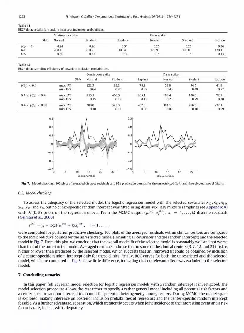
6.3. Model checking

To assess the adequacy of the selected model, the logistic regression model with the selected covariates x12, x13, x21,x24, x31, and x34 but no clinic-specific random intercept was fitted using drum auxiliary mixture sampling (see Appendix A)with N (0, 5) priors on the regression effects. From the MCMC output (µ(m), α(m)i ), m = 1, . . . ,M discrete residuals(Gelman et al., 2000)

r (m)i = yi − logit(µ(m) + xiα(m)i ), i = 1, . . . , n

were computed for posterior predictive checking. 100 plots of the averaged residuals within clinical centers are comparedto the 95% predictive bounds for the unrestrictedmodel (including all covariates and the random intercept) and the selectedmodel in Fig. 7. From this plot, we conclude that the overall model fit of the selectedmodel is reasonably well and not worsethan that of the unrestricted model. Averaged residuals indicate that in some of the clinical centers (3, 7, 12, and 23), risk ishigher or lower than predicted by the selected model, which suggests that an improved fit could be obtained by inclusionof a center-specific random intercept only for these clinics. Finally, ROC curves for both the unrestricted and the selectedmodel, which are compared in Fig. 8, show little difference, indicating that no relevant effect was excluded in the selectedmodel.

7. Concluding remarks

In this paper, full Bayesian model selection for logistic regression models with a random intercept is investigated. Themodel selection procedure allows the researcher to specify a rather general model including all potential risk factors anda center-specific random intercept to account for potential heterogeneity among centers. During MCMC, the model spaceis explored, making inference on posterior inclusion probabilities of regressors and the center-specific random interceptfeasible. As a further advantage, separation, which frequently occurs when joint incidence of the interesting event and a riskfactor is rare, is dealt with adequately.


0.0

0.2

0.4

0.6

0.8

1.0

Sen

sitiv

ity1.0 0.8 0.6 0.4 0.2 0.0

Specificity

selected modelunrestricted model

Fig. 8. ROC curves of the unrestricted and the selected model.

Inference on inclusion/exclusion of the center-specific random intercepts is performed in a reparameterized version ofthe model. This reparameterization allows to use the same priors for an appropriately defined parameter of the randomintercept distribution as for the regression effects, thus leading a convenient MCMC scheme. For all parameters subjectto selection, we compared spike and slab priors with Dirac or absolutely continuous spikes. With the exception of theDirac/normal prior (which was used in Frühwirth-Schnatter and Tüchler (2008); Tüchler (2008) and Wagner and Tüchler(2010)), these priors have not yet been used for variance selection of random intercepts or random effects. Our resultsindicate that for appropriate choices of the spike variance, estimated posterior inclusion probabilities both for regressors aswell as the random intercept correspond closely if the same slab component is used.

Dirac spikes and absolutely continuous spikes require different sampling schemes: marginalization which is necessaryfor Dirac spikes produces less autocorrelated draws but at higher computational cost. The trade-off between better mixingof the MCMC chain and computational cost will not only depend on the number of potential regressors, but also on theirposterior inclusion probabilities, and therefore general conclusions cannot be given. Within each class of spike, we wouldrecommend choosing priors with Student slabs, i.e. either the Dirac/Student or the Student/Student prior. Though MCMCfor priors with Laplace components performs well with regard to integrated autocorrelation times, sampling from the GIG-distribution is too costly in our implementation. With a faster algorithm to produce these draws, these priors could beinteresting competitors. The data situation of the ERCP studymight serve as a benchmark concerning the choice of the spiketype with ESS per second being highest (though only slightly in the worst case) for the Student/Student prior.

Acknowledgments

We thank Sylvia Frühwirth–Schnatter for helpful discussions on the random intercept distribution and two anonymousreviewers and the associate editor for their useful comments.We also acknowledge the contributions of Dr. Christine Kapral(Krankenhaus der Elisabethinen, Linz) and the Austrian Society for Gastroenterology and Hepatology (ÖGGH) in the projectBenchmarking ERCP.

Appendix A

Drum auxiliary mixture samplingJoint sampling of the latent variablesu = (u1, . . . , un) and the component indicators r = (r1, . . . , rn) from p(u, r|µ,α, y)

can be performed by carrying out the following sampling steps:

1. Sample the latent variables ui, i = 1, . . . , n from p(ui|µ,α, θ, βc(i), yi) as

ui = log(λiVi + yi)+ log(1 − Vi + λi(1 − yi)), Vi ∼ U [0, 1] ,

where λi = exp(µ+ xiα+ θβc(i)).2. Sample the component indicator ri from the discrete density p(ri|µ,α, θ, βc(i), ui)

Pr(ri = j|µ,α, θ, βc(i), ui) ∝wj

sjexp

−

12

ui − log λi

sj

2.

The parameters (wj, s2j ), j = 1, . . . , 6 are the weights and variances of the components in the finite mixture approxi-mation and are tabulated in Table 1 of Frühwirth-Schnatter and Frühwirth (2010).

Appendix B. Supplementary data

Supplementary material related to this article can be found online at doi:10.1016/j.csda.2011.06.033.

http://dx.doi.org/doi:10.1016/j.csda.2011.06.033


References

Albert, A., Anderson, J.A., 1984. On the existence of maximum likelihood estimates in logistic regression models. Biometrika 71, 1–10.Barthet,M., Lesavre, N., Desjeux, A., Gasmi,M., Berthezene, P., Berdah, S., Viviand, X., Grimaud, J., 2002. Complications of endoscopic sphincterotomy: results

from a single tertiary referral center. Endoscopy 34, 991–997.Bates, D., Maechler, M., 2010. Lme4: linear mixed-effects models using S4 classes. R Package Version 0.999375-37.Brezger, A., Lang, S., 2006. Generalized structured additive regression based on Bayesian P-splines. Computational Statistics and Data Analysis 50, 967–991.Chen, Z., Dunson, D., 2003. Random effects selection in linear mixed models. Biometrics 59, 762–769.Christensen, M., Matzen, P., Schulze, S., Rosenberg, J., 2004. Complications of ERCP: a prospective study. Gastrointestinal Endoscopy 60, 721–731.Cotton, P.B., Garrow, D.A., Gallagher, J., Romagnuolo, J., 2009. Risk factors for complications after ERCP: a multivariate analysis of 11,497 procedures over

12 years. Gastrointestinal Endoscopy 70, 80–88.Fahrmeir, L., Kneib, T., Konrath, S., 2010. Bayesian regularisation in structured additive regression: a unifying perspective on shrinkage, smoothing and

predictor selection. Statistics and Computing 20, 203–219.Figueiredo, M.A.T., 2003. Adaptive sparseness for supervised learning. IEEE Transactions on Pattern Analysis and Machine Intelligence 25, 1150–1159.Freeman, M.L., Nelson, D.B., Sherman, S., Haber, G.B., Herman, M.E., Dorsher, P.J., Moore, J.P., Fennerty, B.M., Ryan, M.E., Shaw, M.J., Lande, J.D., Pheley, A.M.,

1996. Complications of endoscopic biliary sphincterotomy. The New England Journal of Medicine 335, 909–918.Frühwirth-Schnatter, S., Frühwirth, R., 2010. Data augmentation andMCMC for binary andmultinomial logit models. In: Kneib, T., Tutz, G. (Eds.), Statistical

Modelling and Regression Structures—Festschrift in Honour of Ludwig Fahrmeir. Physica-Verlag, Heidelberg, pp. 111–132.Frühwirth-Schnatter, S., Tüchler, R., 2008. Bayesian parsimonious covariance estimation for hierarchical linear mixedmodels. Statistics and Computing 18,

1–13.Gelman, A., Van Dyk, D.A., Huang, Z., Boscardin, J.W., 2008. Using redundant parameterizations to fit hierarchical models. Journal of Computational and

Graphical Statistics 17, 95–122.Gelman, A., Goegebeur, Y., Tuerlinckx, F., Van Mechelen, I., 2000. Diagnostic checks for discrete data regression models using posterior predictive

simulations. Applied Statistics 49, 247–268.Gelman, A., Jakulin, A., Pittau,M.G., Su, Y.-S., 2008. Aweakly informative default prior distribution for logistic and other regressionmodels. Annals of Applied

Statistics 2, 1360–1383.Genkin, A., Lewis, D.D., Madigan, D., 2007. Large-scale Bayesian logistic regression for text categorization. Technometrics 49, 291–304.George, E.I., McCulloch, R., 1993. Variable selection via Gibbs sampling. Journal of the American Statistical Association 88, 881–889.George, E.I., McCulloch, R., 1997. Approaches for Bayesian variable selection. Statistica Sinica 7, 339–373.Geweke, J., 1996. Variable selection and model comparison in regression. In: Bernardo, J.M., Berger, J.O., Dawid, A.P., Smith, A. (Eds.), Bayesian Statistics

5—Proceedings of the Fifth Valencia International Meeting. Oxford University Press, Oxford, pp. 609–620.Geyer, C., 1992. Practical Markov chain Monte Carlo. Statistical Science 7, 473–511.Griffin, J., Brown, P.J., 2010. Inference with normal-gamma prior distributions in regression problems. Bayesian Analysis 5, 171–188.Heinze, G., 2006. A comparative investigation of methods for logistic regression with separated or nearly separated data. Statistics in Medicine 25,

4216–4226.Heinze, G., Schemper, M., 2002. A solution to the problem of separation in logistic regression. Statistics in Medicine 21, 2409–2419.Ishwaran, H., Rao, S.J., 2003. Detecting differentially expressed genes in microarrays using Bayesian model selection. Journal of the American Statistical

Association 98, 438–455.Ishwaran, H., Rao, S.J., 2005. Spike and slab variable selection; frequentist and Bayesian strategies. Annals of Statistics 33, 730–773.Kapral, C., Duller, C., Wewalka, F., Kerstan, E., Vogel, W., Schreiber, F., 2008. Case volume and outcome of endoscopic retrograde cholangiopancreatography:

results of a nationwide austrian benchmarking project. Endoscopy 40, 625–630.Loperfido, S., Angelini, G., Benedetti, G., Chilovi, F., Costan, F., De Berardinis, F., De Bernardin, M., Ederle, A., Fina, P., Fratton, A., 1998. Major early

complications from diagnostic and therapeutic ERCP: a prospective multicenter study. Gastrointestinal Endoscopy 48, 1–10.Masci, E., Toti, G., Mariani, A., Curioni, S., Lomazzi, A., Dinelli, M., Minoli, G., Crosta, C., Comin, U., Fertitta, A., Prada, A., Rubis Passoni, G., Testoni, P., 2001.

Complications of diagnostic and therapeutic ERCP: a prospective multicenter study. The American Journal of Gastroenterology 96, 417–423.Mitchell, T., Beauchamp, J.J., 1988. Bayesian variable selection in linear regression. Journal of the American Statistical Association 83, 1023–1032.Monahan, J.F., Stefanski, L., 1992. Normal scale mixture approximations to F∗(z) and computation of the logistic normal integral. In: Balakrishnan, N. (Ed.),

Handbook of the Logistic Distribution. Marcel Dekker, New York, pp. 529–549.R Development Core Team, 2010. R: a language and environment for statistical computing. R Foundation for Statistical Computing, Vienna, Austria. ISBN:

3-900051-07-0.Rossi, P., 1996. Existence of Bayes estimators for the binomial logit model. In: Berry, D.A., Chaloner, K.M., Geweke, J.K. (Eds.), Bayesian Analysis in Statistics

and Econometrics. John Wiley & Sons, New York, pp. 91–100.Smith, M., Kohn, R., 1996. Nonparametric regression using Bayesian variable selection. Journal of Econometrics 75, 317–343.Smith, M., Kohn, R., 2002. Parsimonious covariance matrix estimation for longitudinal data. Journal of the American Statistical Association 97, 1141–1153.Tüchler, R., 2008. Bayesian variable selection for logistic models using auxiliary mixture sampling. Journal of Computational and Graphical Statistics 17,

76–94.Wagner, H., Tüchler, R., 2010. Bayesian estimation of random effects models for multivariate responses of mixed data. Computational Statistics and Data

Analysis 54, 1206–1218.

bayesian model selection for logistic regression models with random intercept

Documents