energies

Article

3DHIP-Calculator—A New Tool to Stochastically Assess DeepGeothermal Potential Using the Heat-In-Place Method fromVoxel-Based 3D Geological Models

Guillem Piris 1, Ignasi Herms 2,* , Albert Griera 1 , Montse Colomer 2, Georgina Arnó 2

and Enrique Gomez-Rivas 3

�����������������

Citation: Piris, G.; Herms, I.; Griera,

A.; Colomer, M.; Arnó, G.;

Gomez-Rivas, E. 3DHIP-Calculator—

A New Tool to Stochastically Assess

Deep Geothermal Potential Using the

Heat-In-Place Method from

Voxel-Based 3D Geological Models.

Energies 2021, 14, 7338. https://

doi.org/10.3390/en14217338

Academic Editors: Renato Somma

and Daniela Blessent

Received: 11 September 2021

Accepted: 2 November 2021

Published: 4 November 2021

Publisher’s Note: MDPI stays neutral

with regard to jurisdictional claims in

published maps and institutional affil-

iations.

Copyright: © 2021 by the authors.

Licensee MDPI, Basel, Switzerland.

This article is an open access article

distributed under the terms and

conditions of the Creative Commons

Attribution (CC BY) license (https://

creativecommons.org/licenses/by/

4.0/).

1 Departament de Geologia, Universitat Autònoma de Barcelona (UAB), 08193 Barcelona, Spain;guillem.piris@uab.cat (G.P.); albert.griera@uab.cat (A.G.)

2 Àrea de Recursos Geològics, Institut Cartogràfic i Geològic de Catalunya (ICGC), 08038 Barcelona, Spain;montse.colomer@icgc.cat (M.C.); georgina.arno@icgc.cat (G.A.)

3 Departament de Mineralogia, Petrologia i Geologia Aplicada, Facultat de Ciències de la Terra, Universitat deBarcelona (UB), 08028 Barcelona, Spain; e.gomez-rivas@ub.edu

* Correspondence: ignasi.herms@icgc.cat; Tel.: +34-620-95-92-47

Abstract: The assessment of the deep geothermal potential is an essential task during the earlyphases of any geothermal project. The well-known “Heat-In-Place” volumetric method is the mostwidely used technique to estimate the available stored heat and the recoverable heat fraction ofdeep geothermal reservoirs at the regional scale. Different commercial and open-source softwarepackages have been used to date to estimate these parameters. However, these tools are either notfreely available, can only consider the entire reservoir volume or a specific part as a single-voxelmodel, or are restricted to certain geographical areas. The 3DHIP-Calculator tool presented in thiscontribution is an open-source software designed for the assessment of the deep geothermal potentialat the regional scale using the volumetric method based on a stochastic approach. The tool estimatesthe Heat-In-Place and recoverable thermal energy using 3D geological and 3D thermal voxel modelsas input data. The 3DHIP-Calculator includes an easy-to-use graphical user interface (GUI) forvisualizing and exporting the results to files for further postprocessing, including GIS-based mapgeneration. The use and functionalities of the 3DHIP-Calculator are demonstrated through a casestudy of the Reus-Valls sedimentary basin (NE, Spain).

Keywords: Heat-In-Place; recoverable heat; deep geothermal potential; mapping; MATLAB

1. Introduction

Deep geothermal energy exploration and exploitation activities have vigorously grownduring the last decade worldwide [1–3]. One of the key tasks during the early evalua-tion stages of deep geothermal plays is the assessment of the base resource in terms ofthe energy stored in the reservoir [4]. This quantification is an essential step to estimatethe energy that can be produced from the geothermal reservoir for power generation ordirect uses (district heating, greenhouses, etc.), and is key for carrying out preliminaryevaluations of the project feasibility based on the required investment and the exploita-tion cost of the geothermal resource. However, there are uncertainties in the geologicalknowledge that must be considered when carrying out these preliminary assessmentsduring the early stages of exploration of the geothermal resource. These uncertainties aremainly related to the prediction of the reservoir geometry, petrophysical properties, andtemperature distribution.

The volumetric “Heat-In-Place” (HIP) method, implemented by the United StatesGeological Survey (USGS) [5], together with its subsequent revisions [6–10], is still themost widely used evaluation technique for the estimation of the available stored heat andthe recoverable heat fraction (Hrec) of deep geothermal reservoirs [11–16]. This method

Energies 2021, 14, 7338. https://doi.org/10.3390/en14217338 https://www.mdpi.com/journal/energies

Energies 2021, 14, 7338 2 of 21

considers the volume of the reservoir (surface and thickness), the petrophysical properties(e.g., rock type, porosity, specific heat capacity, etc.), fluid properties (e.g., fluid density, etc.),as well as the reservoir and reinjection (or reference) temperatures. Due to the potentialinfluence of these parameters and their uncertainty, Nathenson [17] considered the needto follow a stochastic approach through Monte Carlo simulations [18]. This approachsystematically varies the parameters considered over a defined range of values by usingprobability distribution functions (PDF) (e.g., triangular, normal, lognormal, etc.) [8,19,20].

Traditionally, common commercial software designed for risk and decision analysispurposes, such as @Risk [21] and Crystal Ball [22], have been used for geothermal re-source assessment. They apply the volumetric method using Monte Carlo simulations (i.e.,stochastic calculations implementing PDFs for the variables). Both tools run as MicrosoftExcel add-ins, and calculations are normally applied at the scale of the entire reservoiror to a specific part of it, where the selected volume is conceptually treated as a singlevoxel [23–26]. In terms of open-source software, Pocasangre et al. [27] have more recentlydeveloped the ‘GPPeval’ application (Geothermal Power Potential assessment), a Python-based stochastic library for the assessment of the geothermal power potential using thevolumetric method in a liquid-dominated reservoir. A handicap of these applicationsis that the analyzed domain must be treated as a lumped parameter model, i.e., with ahomogeneous distribution of parameters in the whole volume considered. However, localvariabilities are expected in reservoirs, mainly due to the variation of the petrophysicalproperties, temperature distribution, and reservoir geometry (thickness, depth, etc.). Forthis reason, approaches based on GIS (Geographic Information System) coupled with 3Dsubsurface models are promising, because they explicitly allow the application of the volu-metric method using 3D voxel models as inputs. Several authors have used 3D geologicalmodels to calculate the volume of a reservoir to subsequently apply the HIP volumetricmethod in a deterministic way by assigning values to parameters of each unit to estimate,quantify, and map a first estimation of the geothermal reserve [28,29].

A more sophisticated approach is that applied by the VIGORThermoGIS code [12],an implementation of the ThermoGIS TNO code [30–32]. This tool was implementedspecifically to assess prospective areas for geothermal development in the Netherlandsand in southern Italy during the VIGOR Project [12]. The codes and the methodologyimplemented in these two tools can be considered nowadays as a reference for the sci-entific community working on the evaluation of resources at the regional scale. Thesetools demonstrated the use of methods that couple 3D subsurface data with GIS tools tostochastically assess the deep geothermal potential. Nevertheless, their implementationwas limited to their case study areas and specific datasets. Therefore, there is still a needfor a standard and freely available tool for the whole geothermal community in order to beable to estimate the HIP using Monte Carlo simulations, and in which any 3D geologicaland 3D thermal models can be utilized to assess case studies.

A gap is identified between what the geoscience community working in geother-mal energy would need (including geological surveys, universities, research institutes, orconsulting companies) and what is currently offered by free commercial or open-source soft-ware packages to assess deep geothermal potential at the regional scale in three-dimensionsand by stochastically using the volumetric method. To close this gap, a novel and freesoftware called the ‘3DHIP-Calculator’ is presented here. This tool allows for estimatingthe geothermal potential of a reservoir using the volumetric Heat-In-Place (HIP) method,originally implemented by the United States Geological Survey (USGS) [5], combined witha Monte Carlo simulation approach [17] and using 3D geological and 3D thermal modelsbased on a voxel format as inputs.

The 3DHIP-Calculator application has many competitive advantages. Firstly, thesource code and the installation files are accessible for all users and developers from open-source repositories such as GitHub. Secondly, as the tool allows importing 3D models thatintegrate previously generated geological, petrophysical, and thermal data, it considersthe whole geological heterogeneity of the reservoir to estimate the geothermal potential

Energies 2021, 14, 7338 3 of 21

using the HIP method. Finally, the results can be exported in ASCII format for theirsubsequent post-processing in other environments, such as GIS software packages. Thisallows generating maps of the assessed deep geothermal potential at the regional scale, andto use 3D visualization tools and statistical packages, such as R [33], for further evaluations.All these advantages open a wide range of possibilities, including the construction ofGIS-based maps or to conduct feasibility studies of the deep geothermal potential throughrisk analysis approaches.

This contribution presents the structure, capabilities, and use of the 3DHIP-Calculatorand its graphical user interface (GUI). Moreover, the method is demonstrated througha case study of the Reus-Valls Basin (RVB) [34]. The RVB is part of the Neogene exten-sional basins of the Catalan Coastal Ranges (NE of the Iberian Peninsula, Spain), which,according to previous studies [35–37], has a high potential for the development of deepgeothermal energy for direct heat or power generation. However, the lack of enoughsubsurface information (from deep appraisal wells) results in a relatively large uncertaintyfor the assessment of its geothermal potential. The RVB case is a useful example of deepgeothermal potential assessment at the regional scale, where the 3DHIP-Calculator canoffer a first estimate of the spatial distribution of the deep geothermal resource based onthe existing geological knowledge and its associated uncertainty.

2. Materials and Methods2.1. Mathematical Background of the HIP Method

The 3DHIP-Calculator is based on the HIP approach, which allows estimating thegeothermal resource and the recoverable fraction of a subsurface reservoir [5,10–12]. TheHIP (kJ) is calculated according to Equation (1):

HIP = V·[∅·ρF·CF + (1 −∅)·ρR·CR]·(Tr − Ti) (1)

where V is the voxel volume (m3), ∅ is the rock porosity (parts per unit), ρ is the rockdensity (kg/m3), C is the specific heat capacity (kJ/kg·◦C), and the F and R sub-indexesaccount for the fluid and host rock, respectively. Tr is the reservoir temperature (◦C) and Tirefers to either the re-injection, reference, or abandonment temperature (◦C). Therefore, Tican refer to the threshold of economic or technological viable temperature, the ambienttemperature (i.e., the annual mean surface temperature value), or a temperature valuedefined according to other criteria [11]. Equation (1) is solved within the 3DHIP-Calculatorfor each voxel in the model that satisfies the condition that (Tr − Ti) ≥ 5 ◦C. Otherwise,the HIP for that voxel is not evaluated and is set to zero. The HIP is expressed in kJ.

Then, the obtained HIP value is used to calculate the recoverable heat (Hrec) followingEquation (2), which accounts for the producible thermal power during a given plant orproject lifetime (Tlive):

Hrec =HIP·Ce·RTlive·P f

(2)

where the HIP resulting from Equation (1) is scaled by a recovery factor (R, in parts perunit) to represent the part of the heat that can be extracted. This first estimation of therecovery factor (R) requires special attention because it depends on many factors, includingthe hydrogeological characteristics of the reservoir and the current drilling technology.Some authors suggest using R values between 0.02 and 0.2 [38] or close to 0.01 [12] forstudies where there is no previous information. A recovery factor for a geothermal doublet(with a production borehole and an injection borehole) was defined at 0.33 according tothe Atlas of Geothermal Resources in Europe [16,39], based on Muffler and Cataldi [5]and Lavigne [40]. Williams et al. [6,7,41] proposed a range of R values according to thegeothermal reservoir type: a range from 0.08 to 0.2 for fracture-dominated reservoirs, 0.01for Enhanced Geothermal Systems [42], and from 0.1 to 0.25 for sediment-hosted reservoirswith a maximum value of 0.5 [3]. Additionally, a conversion efficiency factor (Ce, in partsper unit) is used to incorporate the effect of the efficiency of the heat exchange from the

Energies 2021, 14, 7338 4 of 21

geothermal fluid to a secondary fluid in a thermal plant. Ce can vary as a function ofgeothermal exploitation (e.g., heat or electricity production). Finally, since most of thedirect heat applications of geothermal energy (such as district heating, greenhouse heating,etc.) do not operate continuously throughout the year, a plant factor (Pf, in parts per unit)is included. This factor considers the fraction of the total time in which the geothermalplant is in operation. Thus, Hrec is expressed in kW.

2.2. Mathematical Background of the Monte Carlo Method

The Monte Carlo method, i.e., a multiple probability simulation, is a mathematicalsolution widely used to estimate the possible outcomes of an uncertain event. Unlike anormal forecasting model, Monte Carlo simulations predict a set of outcomes based on anestimated range of values versus a deterministic or fixed input value. This method is used inthe 3DHIP-Calculator to probabilistically evaluate the uncertainty associated with the inputparameters and the corresponding geothermal potential results [18]. The first step is to linka probability distribution function (PDF) to each parameter, to infer the unknown quantitiesof the samples, and to take into account the range and pattern of variation of the differentparameters [43]. Thus, Equations (1) and (2) are applied using a stochastic approach,instead of a deterministic one, so that their input values are not fixed parameters yieldinga unique result. The calculations based on these two equations are repeated as manytimes as desired (N, number of simulations), producing a large number of likely outcomes,using random values extracted from probability distribution functions assigned to theparameters and predefined depending on the pattern variation. The application allowsselecting normal or triangular PDFs for the input parameters of Equations (1) and (2). Themean and standard deviation are used to define normal distributions, while the lower, mostprobable, and upper values are for triangular distributions. The required input data for thecalculations are 3D geological models (3DGM), 3D thermal models (3DTM), and randomvalues within the selected PDF for each parameter. The values of the variables defined in adeterministic way (i.e., without assigning PDFs) are considered as fixed. Accordingly, theapplication calculates as many different HIP and Hrec values as the number of simulationsdefined by the user for each voxel of the model. The results of the calculations are alsoexpressed as PDFs.

2.3. Program Description

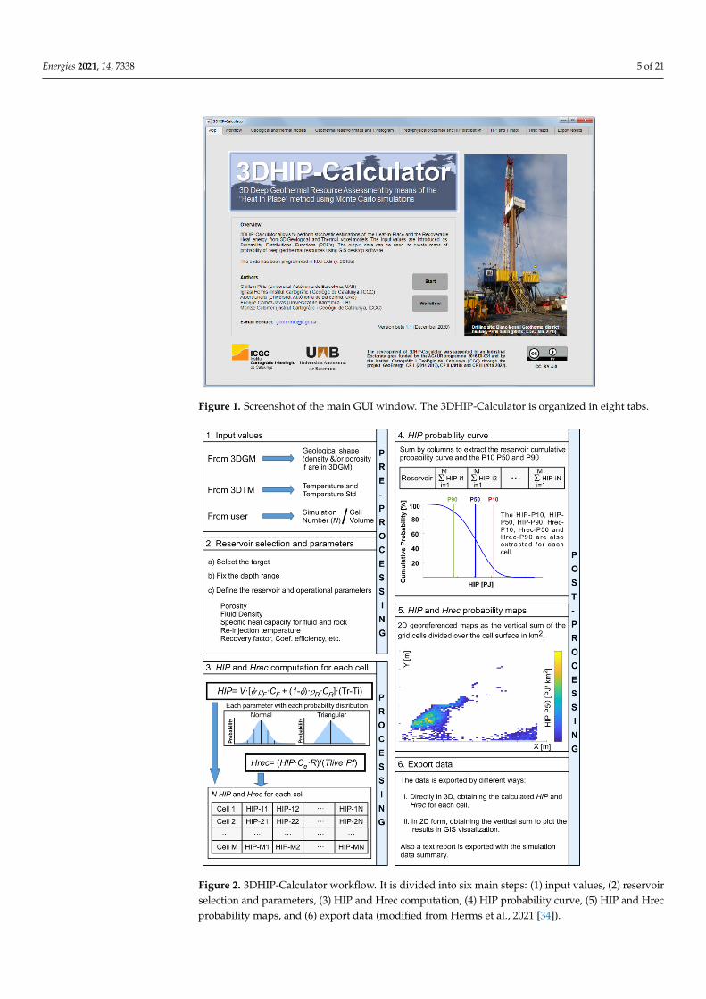
The 3DHIP-Calculator (Figure 1) was developed using MATLAB ® (v. R2019b) [44]based on the MATLAB App Designer, and then compiled for Windows as a standaloneapplication. The installation files, as well as the user manual and examples, can be freelydownloaded from the “Deep geothermal energy” web page of the Institut Cartogràfici Geològic de Catalunya (ICGC) (under the Creative Commons license Attribution 4.0International, CC BY 4.0). The source code can also be downloaded from https://github.com/OpenICGC/3DHIP-Calculator (accessed on 15 October 2021).

An easy-to-use graphical user interface (GUI) was implemented and organized insix main steps, as shown in the workflow of Figure 2. The first part comprises the pre-processing step, that includes the selection of input parameters (step 1 in Figure 2). In thisstep, the input 3D geological and 3D thermal models (referred to as 3DGM and 3DTM,respectively) are converted to a matrix, where each row corresponds to one voxel in the 3Dmodel and the columns are the petrophysical/reservoir parameters. Using depth rangesand geological units, the target volume of the whole model is defined. The parameters thatare not included as initial data in the 3D models are defined using PDFs (2, Figure 2).

Energies 2021, 14, 7338 5 of 21

Figure 1. Screenshot of the main GUI window. The 3DHIP-Calculator is organized in eight tabs.

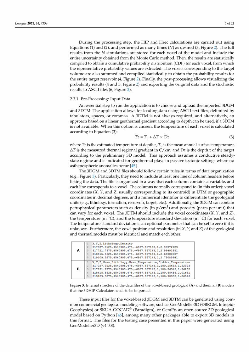
Figure 2. 3DHIP-Calculator workflow. It is divided into six main steps: (1) input values, (2) reservoirselection and parameters, (3) HIP and Hrec computation, (4) HIP probability curve, (5) HIP and Hrecprobability maps, and (6) export data (modified from Herms et al., 2021 [34]).

Energies 2021, 14, 7338 6 of 21

During the processing step, the HIP and Hrec calculations are carried out usingEquations (1) and (2), and performed as many times (N) as desired (3, Figure 2). The fullresults from the N simulations are stored for each voxel of the model and include theentire uncertainty obtained from the Monte Carlo method. Then, the results are statisticallycompiled to obtain a cumulative probability distribution (CDF) for each voxel, from whichthe representative probability values are extracted. The voxels corresponding to the targetvolume are also summed and compiled statistically to obtain the probability results forthe entire target reservoir (4, Figure 2). Finally, the post-processing allows visualizing theprobability results (4 and 5, Figure 2) and exporting the original data and the stochasticresults to ASCII files (6, Figure 2).

2.3.1. Pre-Processing: Input Data

An essential step to run the application is to choose and upload the imported 3DGMand 3DTM. The application allows for loading data using ASCII text files, delimited bytabulators, spaces, or commas. A 3DTM is not always required, and alternatively, anapproach based on a linear geothermal gradient according to depth can be used, if a 3DTMis not available. When this option is chosen, the temperature of each voxel is calculatedaccording to Equation (3):

Tz = T0 + ∆T × Dz (3)

where Tz is the estimated temperature at depth z, T0 is the mean annual surface temperature,∆T is the measured thermal regional gradient in C/km, and Dz is the depth z of the targetaccording to the preliminary 3D model. This approach assumes a conductive steady-state regime and is indicated for geothermal plays in passive tectonic settings where noasthenospheric anomalies occur [45].

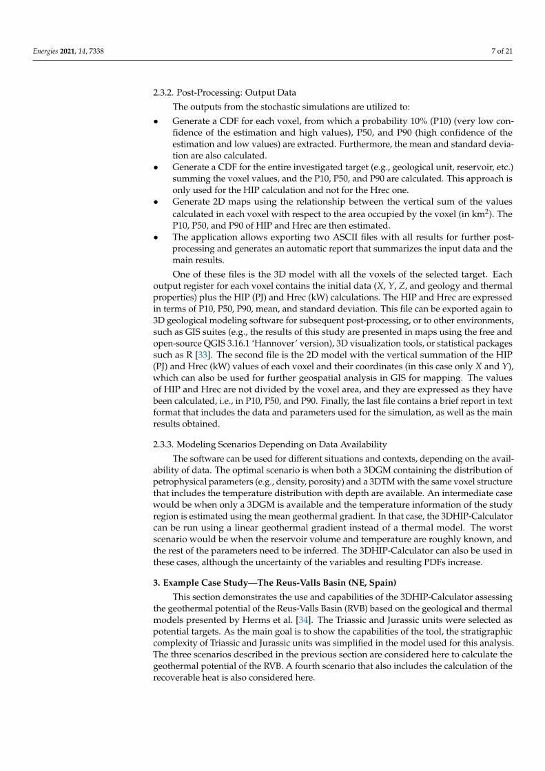
The 3DGM and 3DTM files should follow certain rules in terms of data organization(e.g., Figure 3). Particularly, they need to include at least one line of column headers beforelisting the data. The file is organized in a way that each column contains a variable, andeach line corresponds to a voxel. The columns normally correspond to (in this order): voxelcoordinates (X, Y, and Z, usually corresponding to its centroid) in UTM or geographiccoordinates in decimal degrees, and a numerical identifier to differentiate the geologicalunits (e.g., lithology, formation, reservoir, target, etc.). Additionally, the 3DGM can containpetrophysical parameters such as density (in g/cm3) and porosity (parts per unit) thatcan vary for each voxel. The 3DTM should include the voxel coordinates (X, Y, and Z),the temperature (in ◦C), and the temperature standard deviation (in ◦C) for each voxel.The temperature standard deviation is an optional parameter that can be set to zero if it isunknown. Furthermore, the voxel position and resolution (in X, Y, and Z) of the geologicaland thermal models must be identical and match each other.

Figure 3. Internal structure of the data files of the voxel-based geological (A) and thermal (B) modelsthat the 3DHIP-Calculator needs to be imported.

These input files for the voxel-based 3DGM and 3DTM can be generated using com-mon commercial geological modeling software, such as GeoModeller3D (©BRGM, Intrepid-Geophysics) or SKUA-GOCAD® (Paradigm), or GemPy, an open-source 3D geologicalmodel based on Python [46], among many other packages able to export 3D models inthis format. The files for the testing case presented in this paper were generated usingGeoModeller3D (v4.0.8).

Energies 2021, 14, 7338 7 of 21

2.3.2. Post-Processing: Output Data

The outputs from the stochastic simulations are utilized to:

• Generate a CDF for each voxel, from which a probability 10% (P10) (very low con-fidence of the estimation and high values), P50, and P90 (high confidence of theestimation and low values) are extracted. Furthermore, the mean and standard devia-tion are also calculated.

• Generate a CDF for the entire investigated target (e.g., geological unit, reservoir, etc.)summing the voxel values, and the P10, P50, and P90 are calculated. This approach isonly used for the HIP calculation and not for the Hrec one.

• Generate 2D maps using the relationship between the vertical sum of the valuescalculated in each voxel with respect to the area occupied by the voxel (in km2). TheP10, P50, and P90 of HIP and Hrec are then estimated.

• The application allows exporting two ASCII files with all results for further post-processing and generates an automatic report that summarizes the input data and themain results.

One of these files is the 3D model with all the voxels of the selected target. Eachoutput register for each voxel contains the initial data (X, Y, Z, and geology and thermalproperties) plus the HIP (PJ) and Hrec (kW) calculations. The HIP and Hrec are expressedin terms of P10, P50, P90, mean, and standard deviation. This file can be exported again to3D geological modeling software for subsequent post-processing, or to other environments,such as GIS suites (e.g., the results of this study are presented in maps using the free andopen-source QGIS 3.16.1 ‘Hannover’ version), 3D visualization tools, or statistical packagessuch as R [33]. The second file is the 2D model with the vertical summation of the HIP(PJ) and Hrec (kW) values of each voxel and their coordinates (in this case only X and Y),which can also be used for further geospatial analysis in GIS for mapping. The valuesof HIP and Hrec are not divided by the voxel area, and they are expressed as they havebeen calculated, i.e., in P10, P50, and P90. Finally, the last file contains a brief report in textformat that includes the data and parameters used for the simulation, as well as the mainresults obtained.

2.3.3. Modeling Scenarios Depending on Data Availability

The software can be used for different situations and contexts, depending on the avail-ability of data. The optimal scenario is when both a 3DGM containing the distribution ofpetrophysical parameters (e.g., density, porosity) and a 3DTM with the same voxel structurethat includes the temperature distribution with depth are available. An intermediate casewould be when only a 3DGM is available and the temperature information of the studyregion is estimated using the mean geothermal gradient. In that case, the 3DHIP-Calculatorcan be run using a linear geothermal gradient instead of a thermal model. The worstscenario would be when the reservoir volume and temperature are roughly known, andthe rest of the parameters need to be inferred. The 3DHIP-Calculator can also be used inthese cases, although the uncertainty of the variables and resulting PDFs increase.

3. Example Case Study—The Reus-Valls Basin (NE, Spain)

This section demonstrates the use and capabilities of the 3DHIP-Calculator assessingthe geothermal potential of the Reus-Valls Basin (RVB) based on the geological and thermalmodels presented by Herms et al. [34]. The Triassic and Jurassic units were selected aspotential targets. As the main goal is to show the capabilities of the tool, the stratigraphiccomplexity of Triassic and Jurassic units was simplified in the model used for this analysis.The three scenarios described in the previous section are considered here to calculate thegeothermal potential of the RVB. A fourth scenario that also includes the calculation of therecoverable heat is also considered here.

Energies 2021, 14, 7338 8 of 21

3.1. Geological Setting

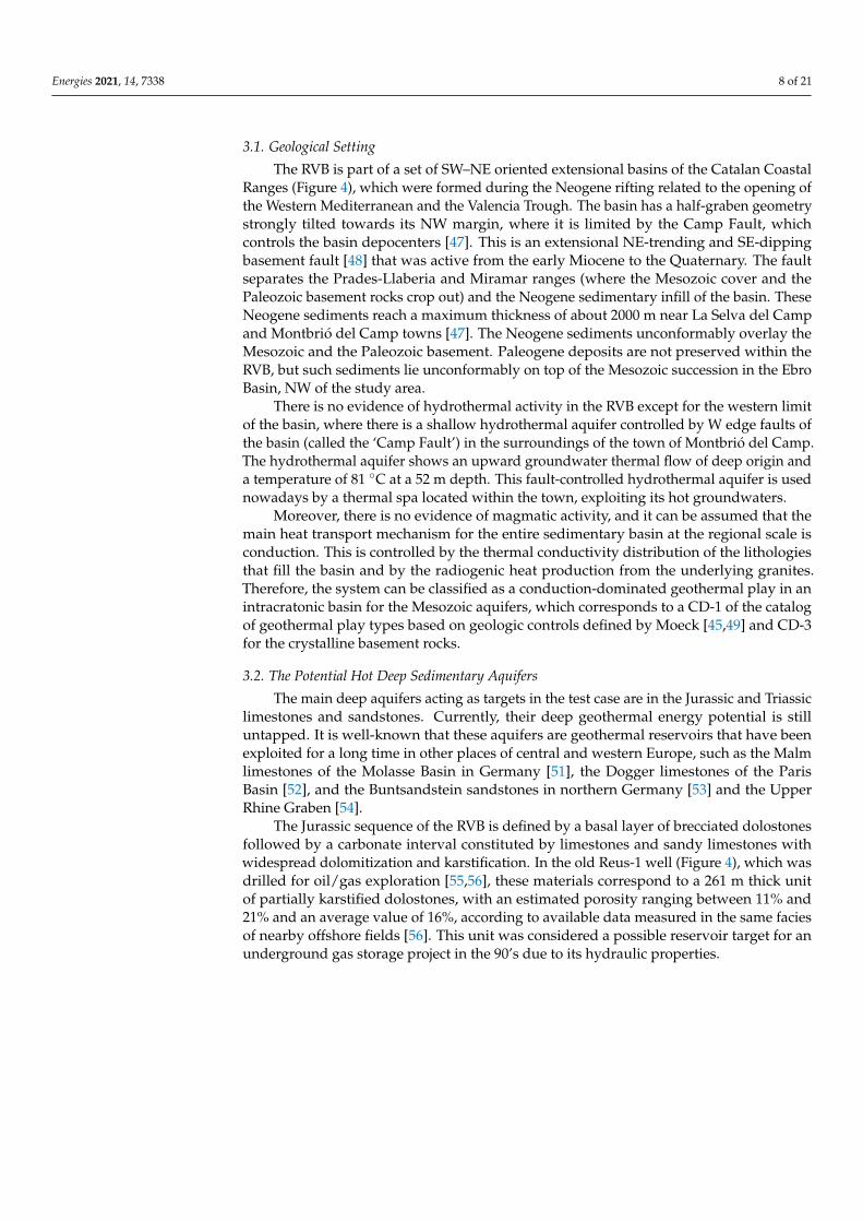
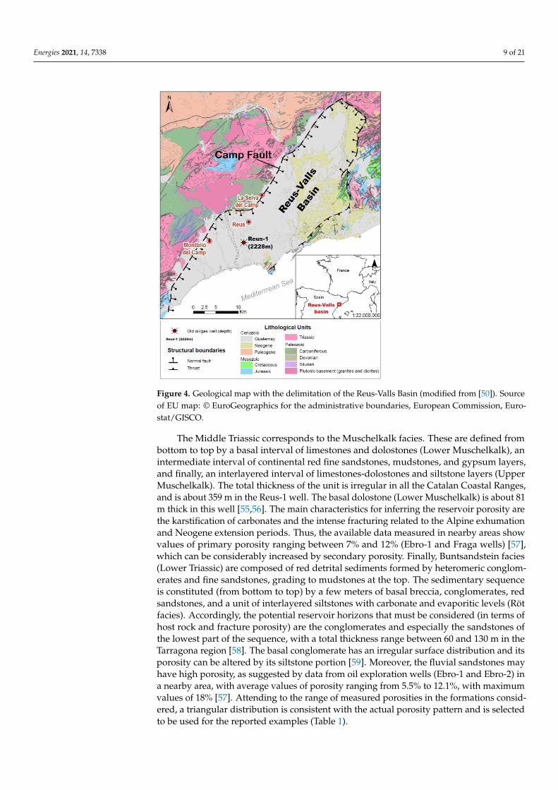
The RVB is part of a set of SW–NE oriented extensional basins of the Catalan CoastalRanges (Figure 4), which were formed during the Neogene rifting related to the opening ofthe Western Mediterranean and the Valencia Trough. The basin has a half-graben geometrystrongly tilted towards its NW margin, where it is limited by the Camp Fault, whichcontrols the basin depocenters [47]. This is an extensional NE-trending and SE-dippingbasement fault [48] that was active from the early Miocene to the Quaternary. The faultseparates the Prades-Llaberia and Miramar ranges (where the Mesozoic cover and thePaleozoic basement rocks crop out) and the Neogene sedimentary infill of the basin. TheseNeogene sediments reach a maximum thickness of about 2000 m near La Selva del Campand Montbrió del Camp towns [47]. The Neogene sediments unconformably overlay theMesozoic and the Paleozoic basement. Paleogene deposits are not preserved within theRVB, but such sediments lie unconformably on top of the Mesozoic succession in the EbroBasin, NW of the study area.

There is no evidence of hydrothermal activity in the RVB except for the western limitof the basin, where there is a shallow hydrothermal aquifer controlled by W edge faults ofthe basin (called the ‘Camp Fault’) in the surroundings of the town of Montbrió del Camp.The hydrothermal aquifer shows an upward groundwater thermal flow of deep origin anda temperature of 81 ◦C at a 52 m depth. This fault-controlled hydrothermal aquifer is usednowadays by a thermal spa located within the town, exploiting its hot groundwaters.

Moreover, there is no evidence of magmatic activity, and it can be assumed that themain heat transport mechanism for the entire sedimentary basin at the regional scale isconduction. This is controlled by the thermal conductivity distribution of the lithologiesthat fill the basin and by the radiogenic heat production from the underlying granites.Therefore, the system can be classified as a conduction-dominated geothermal play in anintracratonic basin for the Mesozoic aquifers, which corresponds to a CD-1 of the catalogof geothermal play types based on geologic controls defined by Moeck [45,49] and CD-3for the crystalline basement rocks.

3.2. The Potential Hot Deep Sedimentary Aquifers

The main deep aquifers acting as targets in the test case are in the Jurassic and Triassiclimestones and sandstones. Currently, their deep geothermal energy potential is stilluntapped. It is well-known that these aquifers are geothermal reservoirs that have beenexploited for a long time in other places of central and western Europe, such as the Malmlimestones of the Molasse Basin in Germany [51], the Dogger limestones of the ParisBasin [52], and the Buntsandstein sandstones in northern Germany [53] and the UpperRhine Graben [54].

The Jurassic sequence of the RVB is defined by a basal layer of brecciated dolostonesfollowed by a carbonate interval constituted by limestones and sandy limestones withwidespread dolomitization and karstification. In the old Reus-1 well (Figure 4), which wasdrilled for oil/gas exploration [55,56], these materials correspond to a 261 m thick unitof partially karstified dolostones, with an estimated porosity ranging between 11% and21% and an average value of 16%, according to available data measured in the same faciesof nearby offshore fields [56]. This unit was considered a possible reservoir target for anunderground gas storage project in the 90’s due to its hydraulic properties.

Energies 2021, 14, 7338 9 of 21

Figure 4. Geological map with the delimitation of the Reus-Valls Basin (modified from [50]). Sourceof EU map: © EuroGeographics for the administrative boundaries, European Commission, Euro-stat/GISCO.

The Middle Triassic corresponds to the Muschelkalk facies. These are defined frombottom to top by a basal interval of limestones and dolostones (Lower Muschelkalk), anintermediate interval of continental red fine sandstones, mudstones, and gypsum layers,and finally, an interlayered interval of limestones-dolostones and siltstone layers (UpperMuschelkalk). The total thickness of the unit is irregular in all the Catalan Coastal Ranges,and is about 359 m in the Reus-1 well. The basal dolostone (Lower Muschelkalk) is about 81m thick in this well [55,56]. The main characteristics for inferring the reservoir porosity arethe karstification of carbonates and the intense fracturing related to the Alpine exhumationand Neogene extension periods. Thus, the available data measured in nearby areas showvalues of primary porosity ranging between 7% and 12% (Ebro-1 and Fraga wells) [57],which can be considerably increased by secondary porosity. Finally, Buntsandstein facies(Lower Triassic) are composed of red detrital sediments formed by heteromeric conglom-erates and fine sandstones, grading to mudstones at the top. The sedimentary sequenceis constituted (from bottom to top) by a few meters of basal breccia, conglomerates, redsandstones, and a unit of interlayered siltstones with carbonate and evaporitic levels (Rötfacies). Accordingly, the potential reservoir horizons that must be considered (in terms ofhost rock and fracture porosity) are the conglomerates and especially the sandstones ofthe lowest part of the sequence, with a total thickness range between 60 and 130 m in theTarragona region [58]. The basal conglomerate has an irregular surface distribution and itsporosity can be altered by its siltstone portion [59]. Moreover, the fluvial sandstones mayhave high porosity, as suggested by data from oil exploration wells (Ebro-1 and Ebro-2) ina nearby area, with average values of porosity ranging from 5.5% to 12.1%, with maximumvalues of 18% [57]. Attending to the range of measured porosities in the formations consid-ered, a triangular distribution is consistent with the actual porosity pattern and is selectedto be used for the reported examples (Table 1).

Energies 2021, 14, 7338 10 of 21

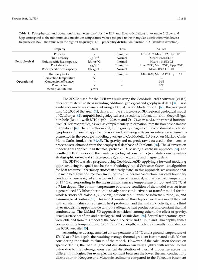
Table 1. Petrophysical and operational parameters used for the HIP and Hrec calculations in example 2 (Low andUpp correspond to the minimum and maximum temperature values assigned to the triangular distribution with lowestfrequencies; Max—the value with the highest frequency; PDF—probability distribution function; SD—standard deviation).

Property Units PDFs Values

Petrophysical

Porosity - Triangular Low: 0.07, Max: 0.12, Upp: 0.18Fluid Density kg/m3 Normal Mean: 1020, SD: 5

Fluid specific heat capacity kJ/kg·◦C Normal Mean: 4.8, SD: 0.1Rock density kg/m3 Triangular Low: 2450, Max: 2500, Upp: 2600

Rock specific heat capacity kJ/kg·◦C Normal Mean: 0.9, SD: 0.01

Operational

Recovery factor - Triangular Min: 0.08, Max: 0.12, Upp: 0.15Reinjection temperature ◦C - 30

Conversion efficiency - - 0.85Plant factor - - 0.95

Mean plant lifetime years - 30

The 3DGM used for the RVB was built using the GeoModeller3D software (v4.0.8)after several iterative steps including additional geological and geophysical data [34]. First,a reference model was generated using a Digital Terrain Model 15 × 15 [60], the geologicalmap 1:50,000 of the area [61], data from the surface-based 3D regional geological modelof Catalunya [62], unpublished geological cross-sections, information from deep oil/gasborehole (Reus-1 well; BTH depth −2228 m and Z: +74.26 m a.s.l.), interpreted horizonsfrom 2D seismic profiles, as well as complementary information from the borehole databaseof Catalonia [63]. To refine this model, a full gravity/magnetic litho-constrained stochasticgeophysical inversion approach was carried out using a Bayesian inference scheme im-plemented in the geologic modeling package of GeoModeller3D based on Markov ChainMonte Carlo simulations [64,65]. The gravity and magnetic raw data used in the inversionprocess were obtained from the geophysical database of Catalonia [66]. The 3D inversionmodeling was applied to fit the most probable 3DGM using a stochastic approach [34]. Theresulted 3DGM honors all the available geological constraints (well data, density values,stratigraphic order, and surface geology), and the gravity and magnetic data.

The 3DTM was also prepared using GeoModeller3D, applying a forward modelingapproach using the quasi-stochastic methodology called Parameter Sweep—an algorithmfor heat resource uncertainty studies in steady-state. In this approach, we assumed thatthe main heat transport mechanism in the basin is thermal conduction. Dirichlet boundaryconditions were assigned at the top and bottom of the model, with a pre-fixed temperatureof 15 ◦C corresponding to the mean annual surface temperature on top, and 176 ◦C ata 7 km depth. The bottom temperature boundary condition of the model was set froma generalized 3D lithospheric scale steady-state conductive heat transfer model for thewhole territory of Catalonia (NE, Spain), previously built with the software LitMod_3D, andassuming local isostasy [67]. This model considered three layers: two layers model the crustwith constant values of radiogenic heat production and thermal conductivity, and a thirdlayer models the upper mantle without radiogenic heat production and constant thermalconductivity. The LitMod_3D approach considers, among others, the effect of gravity,geoid, surface heat flow, and petrological and seismic data [68]. Several temperature layerswere obtained from this model at the base of the crust and at 15, 7, and 3 km depths, with acorresponding temperature of 176 ◦C at a 7 km depth, which are currently published onthe ICGC website [35].

Assuming an average ambient air temperature of 15 ◦C and a ground temperature of176 ◦C at a 7 km depth, the resulting average thermal gradient is estimated at 23 ◦C/kmconsidering the whole thickness of the model. However, if the calculation focuses onspecific depths, the thermal gradient distribution can vary slightly with respect to thisvalue due to the heterogeneous vertical distribution of thermal properties across thedifferent lithologies. For example, the contrast between the lower thermal conductivitydistribution in Neogene and Mesozoic sediments compared to the Paleozoic basement

Energies 2021, 14, 7338 11 of 21

induces a local gradient of 28.3 ◦C/km, from the surface to the top of the Jurassic reservoir inthe Reus-1 well. The petrophysical parameters, i.e., the mean value of thermal conductivity,the heat production rate, and their corresponding standard deviation, for each lithologywere obtained from previous works and the literature [34]. As stated above, the 3DHIP-Calculator can be used in different contexts according to the available data and assumptions.To introduce the different options, different scenarios of data availability were considered.

3.2.1. Example 1: Using a Single-Voxel 1D Geological Model

The first case considered here corresponds to the worst-case scenario, where a voxel-based 3DGM is not available. In this case, we assume an idealized reservoir defined onlyby a single voxel, prepared in a simple way. We impose a fixed value for the reservoirwhole volume and the parameters are defined according to the PDF. This approach can beuseful to obtain a first-order estimation of the HIP when the geometry and temperatureof the target reservoir and the model must be idealized as a single-voxel reservoir. Thiscase is equivalent to those considered in the literature when using commercial applicationssuch as @Risk (Palisade) or Crystal Ball (Oracle) [23–25], and by the ‘GPPeval’ Phyton-based stochastic library [27]. These software packages cannot consider the distributed 3Dgeometry of the reservoirs and therefore must assume the reservoir as a single volume.

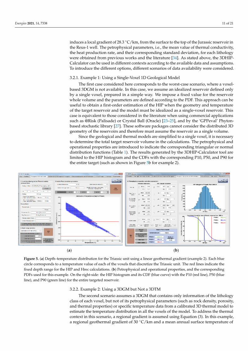
Since the geological and thermal models are simplified to a single voxel, it is necessaryto determine the total target reservoir volume in the calculations. The petrophysical andoperational properties are introduced to indicate the corresponding triangular or normaldistribution functions (Table 1). The results generated by the 3DHIP-Calculator tool arelimited to the HIP histogram and the CDFs with the corresponding P10, P50, and P90 forthe entire target (such as shown in Figure 5b for example 2).

Figure 5. (a) Depth–temperature distribution for the Triassic unit using a linear geothermal gradient (example 2). Each bluecircle corresponds to a temperature value of each of the voxels that discretize the Triassic unit. The red lines indicate thefixed depth range for the HIP and Hrec calculations. (b) Petrophysical and operational properties, and the correspondingPDFs used for this example. On the right-side: the HIP histogram and its CDF (blue curve) with the P10 (red line), P50 (blueline), and P90 (green line) for the entire targeted reservoir.

3.2.2. Example 2: Using a 3DGM but Not a 3DTM

The second scenario assumes a 3DGM that contains only information of the lithologyclass of each voxel, but not of its petrophysical parameters (such as rock density, porosity,and thermal properties) or specific temperature data from a calibrated 3D thermal model toestimate the temperature distribution in all the voxels of the model. To address the thermalcontext in this scenario, a regional gradient is assumed using Equation (3). In this example,a regional geothermal gradient of 30 ◦C/km and a mean annual surface temperature of

Energies 2021, 14, 7338 12 of 21

15 ◦C are assumed. Thus, the depth–temperature profile directly results from Equation (3)(Figure 5a).

After uploading the 3DGM and providing an input value for the geothermal gradient(30 ◦C/km), a total of N = 10,000 realizations were carried out. This number of simulationsis accepted by different authors as high enough for Monte Carlo evaluations [4,19,27,43].For this example, we considered the Triassic unit as the geothermal target reservoir.

The selected depth range of the Triassic reservoir is indicated by two red lines inFigure 5. We selected the lower limit as the bottom of the model, while the upper depthcorresponds to −2000 m a.s.l. The upper depth range was chosen as the limit wherethe reservoir temperature is >60 ◦C, a standard lower cut-off temperature for districtheating stations [69]. The summary of petrophysical and operational properties, and theircorresponding PDFs, are displayed in Table 1 and Figure 5b.

The values of the different parameters have been defined according to the availabledata, as well as from the scientific literature. The range of porosity values for the Buntsand-stein and Muschelkalk units assumes a triangular PDF with porosity values of 7%, 12%,and 18% for the lowest, most probable, and highest values, respectively. Other parameterswere obtained from the general literature, including the fluid density [70], fluid specificheat capacity [71], rock density [72], and rock specific heat capacity [73]. Consideringthe large uncertainty of the recovery factor (R), we used a triangular PDF with a lowervalue of 0.08, a most probable value of 0.12, and an upper value of 0.15, according to aconservative setting.

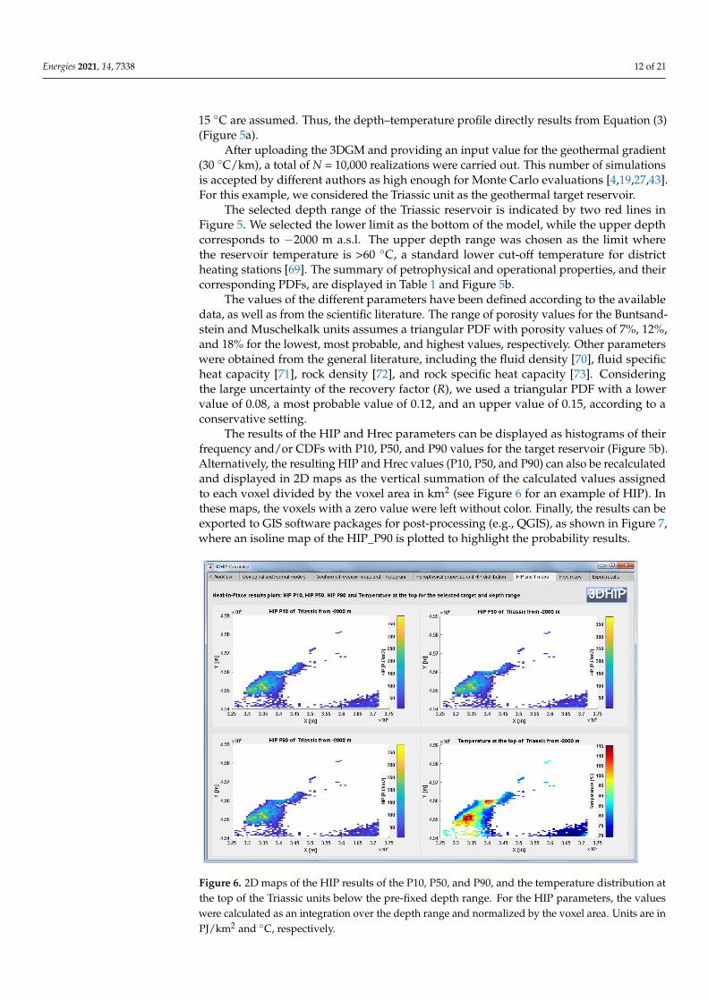
The results of the HIP and Hrec parameters can be displayed as histograms of theirfrequency and/or CDFs with P10, P50, and P90 values for the target reservoir (Figure 5b).Alternatively, the resulting HIP and Hrec values (P10, P50, and P90) can also be recalculatedand displayed in 2D maps as the vertical summation of the calculated values assignedto each voxel divided by the voxel area in km2 (see Figure 6 for an example of HIP). Inthese maps, the voxels with a zero value were left without color. Finally, the results can beexported to GIS software packages for post-processing (e.g., QGIS), as shown in Figure 7,where an isoline map of the HIP_P90 is plotted to highlight the probability results.

Figure 6. 2D maps of the HIP results of the P10, P50, and P90, and the temperature distribution atthe top of the Triassic units below the pre-fixed depth range. For the HIP parameters, the valueswere calculated as an integration over the depth range and normalized by the voxel area. Units are inPJ/km2 and ◦C, respectively.

Energies 2021, 14, 7338 13 of 21

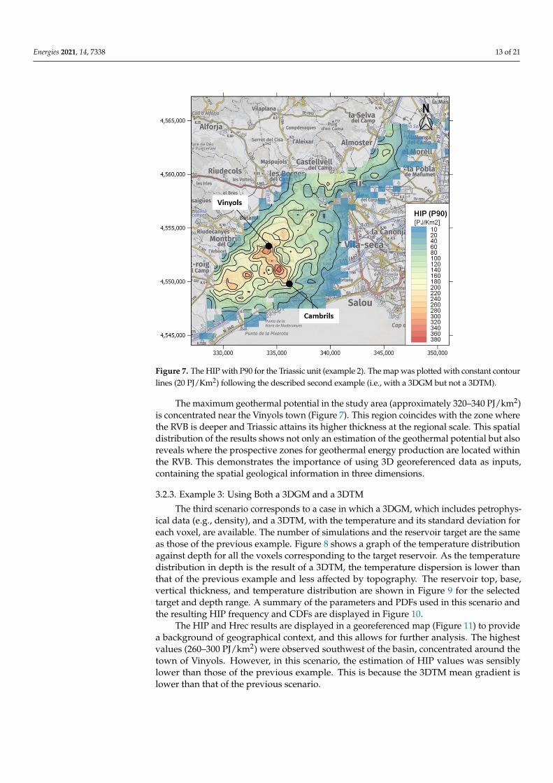
Figure 7. The HIP with P90 for the Triassic unit (example 2). The map was plotted with constant contourlines (20 PJ/Km2) following the described second example (i.e., with a 3DGM but not a 3DTM).

The maximum geothermal potential in the study area (approximately 320–340 PJ/km2)is concentrated near the Vinyols town (Figure 7). This region coincides with the zone wherethe RVB is deeper and Triassic attains its higher thickness at the regional scale. This spatialdistribution of the results shows not only an estimation of the geothermal potential but alsoreveals where the prospective zones for geothermal energy production are located withinthe RVB. This demonstrates the importance of using 3D georeferenced data as inputs,containing the spatial geological information in three dimensions.

3.2.3. Example 3: Using Both a 3DGM and a 3DTM

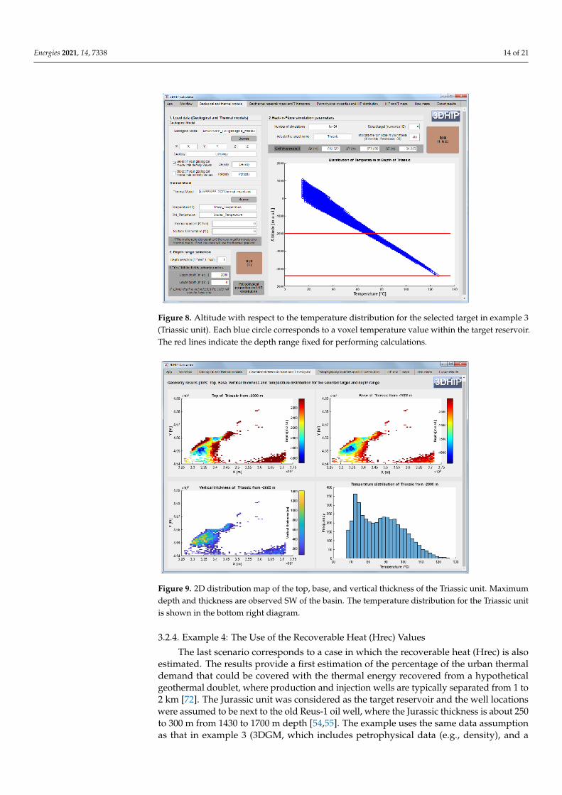
The third scenario corresponds to a case in which a 3DGM, which includes petrophys-ical data (e.g., density), and a 3DTM, with the temperature and its standard deviation foreach voxel, are available. The number of simulations and the reservoir target are the sameas those of the previous example. Figure 8 shows a graph of the temperature distributionagainst depth for all the voxels corresponding to the target reservoir. As the temperaturedistribution in depth is the result of a 3DTM, the temperature dispersion is lower thanthat of the previous example and less affected by topography. The reservoir top, base,vertical thickness, and temperature distribution are shown in Figure 9 for the selectedtarget and depth range. A summary of the parameters and PDFs used in this scenario andthe resulting HIP frequency and CDFs are displayed in Figure 10.

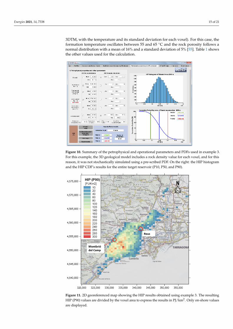
The HIP and Hrec results are displayed in a georeferenced map (Figure 11) to providea background of geographical context, and this allows for further analysis. The highestvalues (260–300 PJ/km2) were observed southwest of the basin, concentrated around thetown of Vinyols. However, in this scenario, the estimation of HIP values was sensiblylower than those of the previous example. This is because the 3DTM mean gradient islower than that of the previous scenario.

Energies 2021, 14, 7338 14 of 21

Figure 8. Altitude with respect to the temperature distribution for the selected target in example 3(Triassic unit). Each blue circle corresponds to a voxel temperature value within the target reservoir.The red lines indicate the depth range fixed for performing calculations.

Figure 9. 2D distribution map of the top, base, and vertical thickness of the Triassic unit. Maximumdepth and thickness are observed SW of the basin. The temperature distribution for the Triassic unitis shown in the bottom right diagram.

3.2.4. Example 4: The Use of the Recoverable Heat (Hrec) Values

The last scenario corresponds to a case in which the recoverable heat (Hrec) is alsoestimated. The results provide a first estimation of the percentage of the urban thermaldemand that could be covered with the thermal energy recovered from a hypotheticalgeothermal doublet, where production and injection wells are typically separated from 1 to2 km [72]. The Jurassic unit was considered as the target reservoir and the well locationswere assumed to be next to the old Reus-1 oil well, where the Jurassic thickness is about 250to 300 m from 1430 to 1700 m depth [54,55]. The example uses the same data assumptionas that in example 3 (3DGM, which includes petrophysical data (e.g., density), and a

Energies 2021, 14, 7338 15 of 21

3DTM, with the temperature and its standard deviation for each voxel). For this case, theformation temperature oscillates between 55 and 65 ◦C and the rock porosity follows anormal distribution with a mean of 16% and a standard deviation of 5% [55]. Table 1 showsthe other values used for the calculation.

Figure 10. Summary of the petrophysical and operational parameters and PDFs used in example 3.For this example, the 3D geological model includes a rock density value for each voxel, and for thisreason, it was not stochastically simulated using a pre-scribed PDF. On the right: the HIP histogramand the HIP CDF’s results for the entire target reservoir (P10, P50, and P90).

Figure 11. 2D georeferenced map showing the HIP results obtained using example 3. The resultingHIP (P90) values are divided by the voxel area to express the results in PJ/km2. Only on-shore valuesare displayed.

Energies 2021, 14, 7338 16 of 21

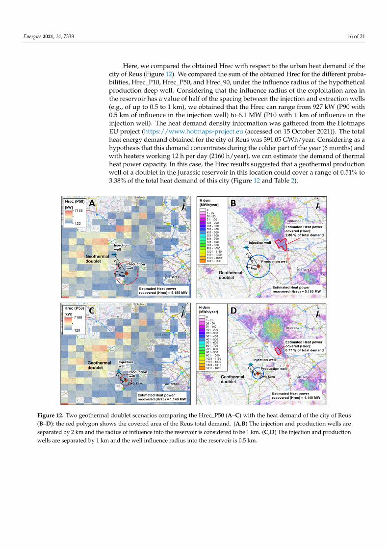
Here, we compared the obtained Hrec with respect to the urban heat demand of thecity of Reus (Figure 12). We compared the sum of the obtained Hrec for the different proba-bilities, Hrec_P10, Hrec_P50, and Hrec_90, under the influence radius of the hypotheticalproduction deep well. Considering that the influence radius of the exploitation area inthe reservoir has a value of half of the spacing between the injection and extraction wells(e.g., of up to 0.5 to 1 km), we obtained that the Hrec can range from 927 kW (P90 with0.5 km of influence in the injection well) to 6.1 MW (P10 with 1 km of influence in theinjection well). The heat demand density information was gathered from the HotmapsEU project (https://www.hotmaps-project.eu (accessed on 15 October 2021)). The totalheat energy demand obtained for the city of Reus was 391.05 GWh/year. Considering as ahypothesis that this demand concentrates during the colder part of the year (6 months) andwith heaters working 12 h per day (2160 h/year), we can estimate the demand of thermalheat power capacity. In this case, the Hrec results suggested that a geothermal productionwell of a doublet in the Jurassic reservoir in this location could cover a range of 0.51% to3.38% of the total heat demand of this city (Figure 12 and Table 2).

Figure 12. Two geothermal doublet scenarios comparing the Hrec_P50 (A–C) with the heat demand of the city of Reus(B–D): the red polygon shows the covered area of the Reus total demand. (A,B) The injection and production wells areseparated by 2 km and the radius of influence into the reservoir is considered to be 1 km. (C,D) The injection and productionwells are separated by 1 km and the well influence radius into the reservoir is 0.5 km.

Energies 2021, 14, 7338 17 of 21

Table 2. Estimated probable heat recovery capacity as a function of the influence radius for ahypothetical geothermal doublet well in the Jurassic reservoir close to the Reus-1 well.

Hrec—Recoverable Heat vs.Estimated R—Radius of Influence Hrec P10 (kWt) Hrec P50 (kWt) Hrec P90 (kWt)

R = 0.5 km 1337 1140 927

R = 1 km 6127 5185 4211

The Hrec results also suggest that the geothermal potential is much higher in thenorthwest of the Reus-1 well. This can be explained due to the fact that to the NW, theJurassic formation lies deeper, up to 2000 m, and thus its temperature, following the 3DTM,oscillates between 70 and 80 ◦C. However, we considered a location close to the Reus-1 oilwell to use its data.

4. Discussion and Conclusions

This paper describes a novel and freely available tool named the 3DHIP-Calculator,which is used to assess the deep geothermal energy potential of hot aquifers. The tool allowsapplying the HIP method to calculate the HIP and the Hrec of a target reservoir followinga Monte Carlo stochastic approach, and using 3D geological and 3D thermal models asinputs. The HIP method [5] is widely known and used in geothermal energy studies. Thetool can be used to generate probability maps, which are of particular importance duringthe preliminary assessment of geothermal resources, mainly at the regional scale. In thiswork, the operation and workflow of the 3DHIP-Calculator tool have been presented. Itsuse has been demonstrated through an example of an area identified with deep geothermalpotential in Mesozoic aquifers located in the NE of the Iberian Peninsula (Reus-Valls Basin),and from considering four different conceptual scenarios based on the available data.

The 3DHIP-Calculator covers the need to have a standard and freely available toolfor the whole geothermal community with which users can estimate the HIP using MonteCarlo simulations and where they can use their 3D models to assess their case studies. Inthis regard, the 3DHIP-Calculator is the only free tool that allows to carry out estimationsof the geothermal potential assessment at the same time, either considering a homogeneousdistribution of parameters (i.e., lumped parameter models) in the whole reservoir orincluding spatial variability of petrophysical properties through the considered reservoir(e.g., density and porosity). Moreover, the 3DHIP-Calculator is not regionally constrainedand can be used to perform geothermal potential assessment exercises independently fromwhere their data is. Additionally, the 3DHIP-Calculator simulations are not limited to aspecific case study and the initial input data can change and incorporate data as these arerefined or obtained through the reservoir characterization. The link between the 3DGMand 3DTM (examples 2 and 3), and the corresponding 3D geothermal potential assessmentmodel (3DGPAM), represents an important step forward with respect to scenarios such asthat of example 1, where the reservoir is represented as a single voxel and the geothermalpotential results are limited to a single CDF with values of P10, P50, and P90 for the entiretarget reservoir, and where the option to include more data as the reservoir knowledgeincreases is truncated.

The results of the 3DGPAM can also again be exported back into 3D geologicalmodeling software to carry out further steps of geothermal exploration of a specific project,or simply exported in 3D visualization software to plot the obtained results (e.g., the open-source, multi-platform data analysis and visualization application, such as ParaView).

The 3DHIP-Calculator is designed to assess and map geothermal resources at theregional scale. It bridges the gap between the first phases of field exploration and geological3D modeling, and the necessary phase of quantification of the geothermal heat availablein deep hot reservoirs, maintaining the uncertainty of the data. Therefore, it should beconsidered a complementary tool to the well-known open-source software DoubletCalc2D [74], which allows calculating the hydraulic performance around geothermal doublets

Energies 2021, 14, 7338 18 of 21

(producing well and injector) over time, and that is also based on stochastic simulations(Monte Carlo). Indeed, this analysis corresponds to a more advanced and detailed phase inthe development of geothermal projects, considering, for example, that it is required formany grant applications related to specific geothermal projects in the Netherlands. The3DHIP-Calculator is not designed to calculate the hydraulic performance of a doublet or todirectly calculate the flow, temperature, and therefore the potential energy recovered fromthem, as other already available tools do for these purposes. However, it is able to make afirst estimation from a hypothetical geothermal doublet, as shown in example 4.

The results obtained in the test case of the Reus-Valls Basin (NE, Spain) demonstratehow the 3DHIP-Calculator can satisfactorily evaluate and map the deep geothermal poten-tial of reservoirs in a distributed manner from 3D models. In the presented test case study,the results reveal the existence of a high geothermal potential located between the villagesof Vinyols and Cambrils (e.g., Figure 7). Although the exploration phase is in a preliminarystage, the results obtained considering the 3D modeling and the stochastic approach willallow progress in the decision-making process for the design of new exploratory campaigns,and thus increase the precision of the predictions. This modeling workflow has improvedthe estimates from previous studies based exclusively on a deterministic and a basin-wideaggregate approach [36,37,75].

The examples presented here demonstrate how geoscientists and engineers can usethe 3DHIP-Calculator to easily evaluate the geothermal potential from their 3D geologicalmodels in a repeatable and systematic manner following a stochastic approach. The toolwill help investors and research organizations determine the suitability of continuing toadvance with new investments in pre-feasibility studies of future deep geothermal projects.

Author Contributions: Conceptualization, G.P.; Methodology, G.P., I.H. and A.G.; Software, G.P.,I.H., A.G., M.C. and E.G.-R.; Resources, M.C. and G.A.; Writing—Original draft preparation, G.P.;Writing—Review and editing, I.H., A.G. and E.G.-R.; Visualization, M.C. and G.A.; Supervision, I.H.,A.G. and E.G.-R. All authors have read and agreed to the published version of the manuscript.

Funding: G.P. was supported by Agència de Gestió d’Ajuts Universitaris i de Recerca (AGAUR) forIndustry Doctorate Research 2016-DI-031 grant and by Institut Cartogràfic i Geològic de Catalunya(ICGC) through the MoU06092016ICGC-UAB and by the MoU11112019ICGC-UAB. E.G.-R. acknowl-edges the support of the Ramón y Cajal fellowship funded by the Spanish Ministry of Science,Innovation and Universities (RYC2018-026335-I and PID2020-118999GB-I00).

Institutional Review Board Statement: Not applicable.

Informed Consent Statement: Not applicable.

Data Availability Statement: The source code can be download from the following GitHub repos-itory: https://github.com/OpenICGC/3DHIP-Calculator (accessed on 15 October 2021) mail forcontact: geotermia@icgc.cat. The installation files, as well as the user manual in PDF format andsome examples for testing the tool, can also be freely downloaded from the Deep geothermal energyweb page of the Institut Cartogràfic i Geològic de Catalunya (ICGC) (under the Creative Commonslicense Attribution 4.0 International, CC BY 4.0).

Acknowledgments: The 3DHIP-Calculator software was developed during a PhD grant of theIndustrial Doctorate programme sponsored by the AGAUR (Agència de Gestió d’Ajuts Universitarisi de Recerca) of the Government of Catalonia (reference number 2016-DI-031), and funded andmaintained by the Institut Cartogràfic i Geològic de Catalunya (ICGC) under the project GeoEnergyof the CP-I (2014–2017), CP-II (2018), and CP-III (2019–2022). E.G.-R. acknowledges the SpanishMinistry of Science, Innovation and Universities for the “Ramón y Cajal” fellowship RYC2018-026335-I and research project PID2020-118999GB-I00. We thank the anonymous reviewers for theirconstructive comments and suggestions which led to a substantial improvement of the paper as wellas all the researchers that has collaborated in this research.

Conflicts of Interest: The authors declare no conflict of interest.

Energies 2021, 14, 7338 19 of 21

References1. Bertani, R. Geothermal Power Generation in the World 2010–2015 Update Report. In Proceedings of the World Geothermal

Congress 2015, Melbourne, Australia, 19–25 April 2015; pp. 19–25.2. Sigfússon, B.; Uihlein, A. 2015 JRC Geothermal Energy Status Report; EUR 27623 EN; Joint Research Center: Petten, The Netherlands,

2015; p. 59. [CrossRef]3. Van Wees, J.-D.; Boxem, T.; Angelino, L.; Dumas, P. A Prospective Study on the Geothermal Potential in the EU. GEOLEC Project; EC:

Utrecht, The Netherlands, 2013; p. 97.4. Agemar, T.; Weber, J.; Moeck, I. Assessment and Public Reporting of Geothermal Resources in Germany: Review and Outlook.

Energies 2018, 11, 332. [CrossRef]5. Muffler, P.; Cataldi, R. Methods for Regional Assessment of Geothermal Resources. Geothermics 1978, 7, 53–89. [CrossRef]6. Williams, C.F. Updated Methods for Estimating Recovery Factors for Geothermal Resources. In Proceedings of the Thirty-Second

Workshop on Proceedings, Geothermal Reservoir Engineering, Stanford University, Stanford, CA, USA, 22 January 2007; p. 7.7. Williams, C.F.; Reed, M.J.; Mariner, R.H. A Review of Methods Applied by the U.S. Geological Survey in the Assessment of Identified

Geothermal Resources; U.S. Geological Survey: Reston, VA, USA, 2008; p. 30.8. Garg, S.K.; Combs, J. Appropriate Use of USGS Volumetric “Heat in Place” Method and Monte Carlo Calculations. In Proceedings

of the Thirty-Fourth Workshop on Geothermal Reservoir Engineering, Stanford University, Stanford, CA, USA, 1 February 2010;p. 7.

9. Garg, S.K.; Combs, J. A Reexamination of USGS Volumetric “Heat in Place” Method. In Proceedings of the Thirty-Sixth Workshopon Geothermal Reservoir Engineering, Stanford University, Stanford, CA, USA, 31 February 2011; p. 5.

10. Garg, S.K.; Combs, J. A Reformulation of USGS Volumetric “Heat in Place” Resource Estimation Method. Geothermics 2015,55, 150–158. [CrossRef]

11. Limberger, J.; Boxem, T.; Pluymaekers, M.; Bruhn, D.; Manzella, A.; Calcagno, P.; Beekman, F.; Cloetingh, S.; van Wees, J.-D.Geothermal Energy in Deep Aquifers: A Global Assessment of the Resource Base for Direct Heat Utilization. Renew. Sustain.Energy Rev. 2018, 82, 961–975. [CrossRef]

12. Trumpy, E.; Botteghi, S.; Caiozzi, F.; Donato, A.; Gola, G.; Montanari, D.; Pluymaekers, M.P.D.; Santilano, A.; van Wees, J.D.;Manzella, A. Geothermal Potential Assessment for a Low Carbon Strategy: A New Systematic Approach Applied in SouthernItaly. Energy 2016, 103, 167–181. [CrossRef]

13. Miranda, M.M.; Raymond, J.; Dezayes, C. Uncertainty and Risk Evaluation of Deep Geothermal Energy Source for HeatProduction and Electricity Generation in Remote Northern Regions. Energies 2020, 13, 4221. [CrossRef]

14. Arango-Galván, C.; Prol-Ledesma, R.M.; Torres-Vera, M.A. Geothermal Prospects in the Baja California Peninsula. Geothermics2015, 55, 39–57. [CrossRef]

15. Pol-Ledesma, R.-M.; Carrillo-de la Cruz, J.-L.; Torres-Vera, M.-A.; Membrillo-Abad, A.-S.; Espinoza-Ojeda, O.-M. Heat Flow Mapand Geothermal Resources in Mexico / Mapa de Flujo de Calor y Recursos Geotérmicos de México. Terra Digit. 2018. [CrossRef]

16. Hurter, S.; Schellschmidt, R. Atlas of Geothermal Resources in Europe. Geothermics 2003, 32, 779–787. [CrossRef]17. Nathenson, M. Methodology of Determining the Uncertainty in the Accessible Geothermal Resource Base of Identified Hydrothermal

Convec-Tion Systems; Open-File Report; U.S. Geological Survey: Menlo Park, CA, USA, 1978; p. 51.18. Rubinstein, R.Y.; Kroese, D.P. Simulation and the Monte Carlo Method, 3rd ed.; Wiley Series in Probability and Statistics; Wiley:

Hoboken, NJ, USA, 2017; ISBN 978-1-118-63220-8.19. Shah, M.; Vaidya, D.; Sircar, A. Using Monte Carlo Simulation to Estimate Geothermal Resource in Dholera Geothermal Field,

Gujarat, India. Multiscale Multidiscip. Model. Exp. Des. 2018, 1, 83–95. [CrossRef]20. Trota, A.; Ferreira, P.; Gomes, L.; Cabral, J.; Kallberg, P. Power Production Estimates from Geothermal Resources by Means of

Small-Size Compact Climeon Heat Power Converters: Case Studies from Portugal (Sete Cidades, Azores and Longroiva Spa,Mainland). Energies 2019, 12, 2838. [CrossRef]

21. Palisade Corporation. @Risk for Excel; Palisade Corporation: Ithaca, NY, USA, 2014.22. Oracle. Oracle Crystal Ball Spreadsheet Functions for Use in Microsoft Excel Models; Oracle: Austin, TX, USA, 2014.23. Arkan, S.; Parlaktuna, M. Resource Assessment of Balçova Geothermal Field. In Proceedings of the World Geothermal Congress

2005, Antalya, Turkey, 24–29 April 2005.24. Yang, F.; Liu, S.; Liu, J.; Pang, Z.; Zhou, D. Combined Monte Carlo Simulation and Geological Modeling for Geothermal Resource

Assessment: A Case Study of the Xiongxian Geothermal Field, China. In Proceedings of the World Geothermal Congress 2015,Melbourne, Australia, 19–25 April 2015; pp. 19–25.

25. Halcon, R.M.; Kaya, E.; Penarroyo, F. Resource Assessment Review of the Daklan Geothermal Prospect, Benguet, Philippines. InProceedings of the World Geothermal Congress 2015, Melbourne, Australia, 19–25 April 2015; pp. 19–25.

26. Barkaoui, A.-E.; Zarhloule, Y.; Varbanov, P.S.; Klemes, J.J. Geothermal Power Potential Assessment in North Eastern Morocco.Chem. Eng. Trans. 2017, 61, 1627–1632. [CrossRef]

27. Pocasangre, C.; Fujimitsu, Y. Geothermics A Python-Based Stochastic Library for Assessing Geothermal Power Potential Usingthe Volumetric Method in a Liquid-Dominated Reservoir. Geothermics 2018, 76, 164–176. [CrossRef]

28. Zhu, Z.; Lei, X.; Xu, N.; Shao, D.; Jiang, X.; Wu, X. Integration of 3D Geological Modeling and Geothermal Field Analysis for theEvaluation of Geothermal Reserves in the Northwest of Beijing Plain, China. Water 2020, 12, 638. [CrossRef]

Energies 2021, 14, 7338 20 of 21

29. Calcagno, P.; Baujard, C.; Dagallier, A.; Guillou-Frottier, L.; Genter, A. Three-Dimensional Estimation of Geothermal Potentialfrom Geological Field Data: The Limagne Geothermal Reservoir Case Study (France). In Proceedings of the Geothermal ResourcesCouncil GRC Annual Meeting, Reno, NV, USA, 4–7 October 2009; p. 326.

30. Van Wees, J.-D.; Juez-Larre, J.; Bonte, D.; Mijnlieff, H.; Kronimus, A.; Gesse, S.; Obdam, A.; Verweij, H. ThermoGIS: An IntegratedWeb-Based Information System for Geothermal Exploration and Governmental Decision Support for Mature Oil and Gas Basins.In Proceedings of the World Geothermal Congress 2010, Bali, Indonesia, 25 April 2010; p. 7.

31. Kramers, L.; van Wees, J.-D.; Pluymaekers, M.P.D.; Kronimus, A.; Boxem, T. Direct Heat Resource Assessment and SubsurfaceInformation Systems for Geothermal Aquifers; the Dutch Perspective. Neth. J. Geosci. 2012, 91, 637–649. [CrossRef]

32. Vrijlandt, M.A.W.; Struijk, E.L.M.; Brunner, L.G.; Veldkamp, J.G.; Witmans, N.; Maljers, D.; van Wees, J.D. ThermoGIS Update:A Renewed View on Geothermal Potential in the Netherlands. In Proceedings of the European Geothermal Congress 2019, TheHague, The Netherlands, 11 June 2019; p. 10.

33. R Core Team. R: A Language and Environment for Statistical Computing; R Foundation for Statistical Computing: Vienna,Austria, 2013.

34. Herms, I.; Piris, G.; Colomer, M.; Peigney, C.; Griera, A.; Ledo, J. 3D Numerical Modelling Combined with a Stochastic Approachin a MATLAB-Based Tool to Assess Deep Geothermal Potential in Catalonia: The Case Test Study of the Reus-Valls Basin. InProceedings of the World Geothermal Congress 2020 + 1, Reykjavik, Iceland, 24–27 October 2021; p. 9.

35. ICGC. Geothermal Atlas of Catalonia: Geoindex-Deep-Geothermal. 2020. Available online: https://www.icgc.cat/en/Public-Administration-and-Enterprises/Tools/Geoindex-viewers/Geoindex-Deep-geothermal-energy (accessed on 15 October 2021).

36. Colmenar-Santos, A.; Folch-Calvo, M.; Rosales-Asensio, E.; Borge-Diez, D. The Geothermal Potential in Spain. Renew. Sustain.Energy Rev. 2016, 56, 865–886. [CrossRef]

37. Arrizabalaga, I.; De Gregorio, M.; De Santiago, C.; Pérez, P. Geothermal Energy Use, Country Update for Spain. In Proceedings ofthe European Geothermal Congress 2019, The Hague, The Netherlands, 11 June 2019; p. 9.

38. Beardsmore, G.R.; Rybach, L.; Blackwell, D.; Baron, C. A Protocol for Estimating and Mapping Global EGS Potential. Geotherm.Resour. Counc. Trans. 2010, 34, 301–312.

39. Hurter, S.; Haenel, R. Atlas of Geothermal Resources in Europe; Official Publications of the European Communities, EuropeanCommission: Luxembourg, 2002.

40. Lavigne, J. Les Resources Geothérmiques Françaises-Possibilités de Mise En Valeur. Ann. Mines 1977, 57–72.41. Williams, C.F. Development of Revised Techniques for Assessing Geothermal Resources. In Proceedings of the Twenty-Ninth

Workshop on Geothermal Reservoir Engineering, Stanford University, Stanford, CA, USA, 26 January 2004; p. 5.42. Lund, J.W.; Boyd, T.L. Direct Utilization of Geothermal Energy 2015 Worldwide Review. Geothermics 2016, 60, 66–93. [CrossRef]43. Wang, Y.; Wang, L.; Bai, Y.; Wang, Z.; Hu, J.; Hu, D.; Wang, Y.; Hu, S. Assessment of Geothermal Resources in the North Jiangsu

Basin, East China, Using Monte Carlo Simulation. Energies 2021, 14, 259. [CrossRef]44. MathWorks. MATLAB; The MathWorks, Inc.: Natick, MA, USA, 2019.45. Moeck, I.; Beardsmore, G.R. A New ‘Geothermal Play Type’ Catalog: Streamlining Exploration Decision Making. In Proceedings

of the Thirty-Ninth Workshop on Geothermal Reservoir Engineering, Stanford University, Stanford, CA, USA, 24 February 2014;p. 8.

46. De la Varga, M.; Schaaf, A.; Wellmann, F. GemPy 1.0: Open-Source Stochastic Geological Modeling and Inversion. Geosci. ModelDev. 2019, 12, 1–32. [CrossRef]

47. Massana, E. L’activitat Neotectònica a Les Cadenes Costaneres Catalanes. Ph.D. Thesis, University of Barcelona, Barcelona, Spain,1995.

48. Cabrera, L.; Calvet, F. Onshore Neogene record in NE Spain: Vallès–Penedès and El Camp half-grabens (NW Mediterranean).In Tertiary Basins of Spain; Friend, P.F., Dabrio, C.J., Eds.; Cambridge University Press: Cambridge, UK, 1996; pp. 97–105,ISBN 978-0-521-46171-9.

49. Moeck, I.S. Catalog of Geothermal Play Types Based on Geologic Controls. Renew. Sustain. Energy Rev. 2014, 37, 867–882.[CrossRef]

50. ICGC. Base Geològica 1:50,000 de Catalunya. Available online: https://www.icgc.cat/en/Public-Administration-and-Enterprises/Downloads/Geological-and-geothematic-cartography/Geological-cartography/Geological-map-1-50-000 (accessedon 1 January 2021).

51. Moeck, I.S.; Dussel, M.; Weber, J.; Schintgen, T.; Wolfgramm, M. Geothermal Play Typing in Germany, Case Study Molasse Basin:A Modern Concept to Categorise Geothermal Resources Related to Crustal Permeability. Neth. J. Geosci. 2019, 98, e14. [CrossRef]

52. Lopez, S.; Hamm, V.; Le Brun, M.; Schaper, L.; Boissier, F.; Cotiche, C.; Giuglaris, E. 40 Years of Dogger Aquifer Management inIle-de-France, Paris Basin, France. Geothermics 2010, 39, 339–356. [CrossRef]

53. Blöcher, G.; Reinsch, T.; Henninges, J.; Milsch, H.; Regenspurg, S.; Kummerow, J.; Francke, H.; Kranz, S.; Saadat, A.; Zimmermann,G.; et al. Hydraulic History and Current State of the Deep Geothermal Reservoir Groß Schönebeck. Geothermics 2016, 63, 27–43.[CrossRef]

54. Haffen, S.; Géraud, Y.; Diraison, M.; Dezayes, C.; Siffert, D.; Garcia, M. Temperature Gradient Anomalies in the BuntsandsteinSandstone Reservoir, Upper Rhine Graben, Soultz, France. In Proceedings of the Tu D203 09—76th EAGE Conference & Exhibition2014, Amsterdam, The Netherlands, 16 June 2014.

Energies 2021, 14, 7338 21 of 21

55. Zapatero, M.A.; Reyes, J.L.; Martínez, R.; Suárez, I.; Arenillas, A.; Perucha, M.A. Estudio Preliminar de las Formaciones Favorablespara el Almacenamiento Subterráneo de CO2 en España; Instituto Geológico y Minero de España (IGME): Madrid, Spain, 2009; p. 135.

56. AURENSA. Proyecto de Almacenamientos Subterraneos de Gas. Reus; Auxiliar de Recursos y Energía, S.A.: Madrid, Spain, 1996;p. 65.

57. Campos, R.; Recreo, F.; Perucha, M.A. AGP de CO2: Selección de Formaciones Favorables en la Cuenca del Ebro; Informes TécnicosCiemat; CIEMAT: Madrid, España, 2007; p. 124.

58. Marzo, M. El Bundstandstein de los Catalánides: Estratigrafía y Procesos Sedimentarios. Ph.D. Thesis, Universitat de Barcelona,Barcelona, Spain, 1980.

59. Zapatero, M.A.; Suárez, I.; Arenillas, A.; Marina, M.; Catalina, R.; Martínez-Orío, R. Proyecto Europeo GeoCapacity. AssessingEuropean Capacity for Geological Storage of Carbon Dioxide; Instituto Geológico y Minero de España (IGME): Madrid, España, 2009;p. 162.

60. ICGC. Model d’Elevacions Del Terreny de Catalunya 15 × 15 Metres (MET-15) v2.0. 2018. Available online: https://www.icgc.cat/Descarregues/Elevacions/Model-d-elevacions-del-terreny-de-15x15-m (accessed on 11 January 2021).

61. ICGC. Mapa Geològic Comarcal de Catalunya. Full Del Baix Camp. 2006. Available online: https://www.icgc.cat/en/Public-Administration-and-Enterprises/Downloads/Geological-and-geothematic-cartography/Geological-cartography/Geological-map-1-50-000 (accessed on 11 January 2021).

62. ICGC. Model 3D Geològic de Catalunya. 2013. Available online: https://www.icgc.cat/ca/Administracio-i-empresa/Descarregues/Cartografia-geologica-i-geotematica/Cartografia-geologica/Model-geologic-3D-de-Catalunya (accessed on15 January 2020).

63. ICGC. Base de Dades de Sondejos de Catalunya (BDSoC). 2015. Available online: https://www.icgc.cat/ca/Administracio-i-empresa/Eines/Visualitzadors-Geoindex/Geoindex-Prospeccions-geotecniques (accessed on 15 January 2020).

64. Scott, S.W.; Covell, C.; Júlíusson, E.; Valfells, Á.; Newson, J.; Hrafnkelsson, B.; Pálsson, H.; Gudjónsdóttir, M. A ProbabilisticGeologic Model of the Krafla Geothermal System Constrained by Gravimetric Data. Geotherm. Energy 2019, 7, 29. [CrossRef]

65. Scott, S.; Covell, C.; Juliusson, E.; Valfells, Á.; Newson, J.; Hrafnkelsson, B.; Pálsson, H.; Gudjónsdóttir, M. A ProbabilisticGeologic Model of the Krafla Geothermal System Based on Bayesian Inversion of Gravimetric Data. In Proceedings of the WorldGeothermal Congress 2020 + 1, Reykjavik, Iceland, 24–27 October 2021; p. 13.

66. ICGC. Base de Dades Geofísica de Catalunya. 2013. Available online: https://www.icgc.cat/Administracio-i-empresa/Serveis/Geofisica-aplicada/Geoindex-Tecniques-geofisiques (accessed on 15 January 2020).

67. Fullea, J.; Afonso, J.C.; Connolly, J.A.D.; Fernàndez, M.; García-Castellanos, D.; Zeyen, H. LitMod3D: An Interactive 3-D Softwareto Model the Thermal, Compositional, Density, Seismological, and Rheological Structure of the Lithosphere and SublithosphericUpper Mantle: LITMOD3D-3-D Interactive code to model lithosphere. Geochem. Geophys. Geosyst. 2009, 10. [CrossRef]

68. Carballo, A.; Fernández, M.; Jiménez-Munt, I. Corte Litosférico al Este de La Península Ibérica y Sus Márgenes. Modelización deLas Propiedades Físicas Del Manto Superior. Física Tierra 2011, 23, 131–147. [CrossRef]

69. Agemar, T.; Weber, J.; Schulz, R. Deep Geothermal Energy Production in Germany. Energies 2014, 7, 4397–4416. [CrossRef]70. Oldenburg, C.M.; Rinaldi, A.P. Buoyancy Effects on Upward Brine Displacement Caused by CO2 Injection. Transp. Porous Media

2011, 87, 525–540. [CrossRef]71. Lukosevicius, V. Thermal Energy Production from Low Temperature Geothermal Brine—Technological Aspects and Energy Efficiency;

ONU Geothermal Training Programme; Orkustofnum—National Energy Authority: Grensasvegur, Reykjavik, Iceland, 1993;p. 42.

72. Ayala, C. Basement Characterisation and Cover Deformation of the Linking Zone (NE Spain) from 2.5D and 3D Geological andGeophysical Modelling. In Proceedings of the 8th EUREGEO, Barcelona, Spain, 15–17 June 2015; p. 23.

73. Willems, C.J.L.; Nick, H.M. Towards Optimisation of Geothermal Heat Recovery: An Example from the West Netherlands Basin.Appl. Energy 2019, 247, 582–593. [CrossRef]

74. Veldkamp, J.G.; Pluymaekers, M.P.D.; van Wees, J.-D. DoubletCalc 2D (v1.0) Manual; TNO 2015 R10216; TNO: Utrecht, TheNetherlands, 2015.

75. Arrizabalaga, I.; De Gregorio, M.; De Santiago, C.; García de la Noceda, C.; Pérez, P.; Urchueguía, J.F. Country Update for theSpanish Geothermal Sector. In Proceedings of the World Geothermal Congress 2020 + 1, Reykjavik, Iceland, 24–27 October 2021.