2019 user's manual - forensic mathematics
TRANSCRIPT
DNA·VIEW®
2019
User’s Manual
revised June 15, 2015
program version 37.06
English
Charles Brenner
6801 Thornhill Drive
Oakland, California 94611-1336
(510)339-1911 fax (510)339-1181
email: [email protected]
website: http://www.dna-view.com
Introductory Guide
Installation: To install use either the installation CD or installation file downloaded from the Internet. The
CD should autostart. In either case the installation file has a name like setupDNAVIEW37.06 ...exe,
which can be invoked by browsing with Windows’ “My Computer” if necessary.
There may be a password necessary as part of the installation. Qualified users may obtain it by asking.
See §XV.A, page 295.
Startup Normally installation creates desktop icons for starting the program.
See §XV.E, page 303.
Contact for information, inquiries, or
problems
Overview of DNA@VIEW — §I.E (page 22) and chapter II (page 29).®
Recent changes in this manual and in DNA@VIEW — page 3.
Updates through the Internet:
Visit the Forensic Mathematics downloads page, http://dna-view.com/downloads.
Click on and save a file with a name like setupDNAVIEW37.06update.exe.
Request the password.
See Installation above.
Update disks/CD’s available on request.
W:\dnadoc\DNAVIEW 2019 US.wpd Copyright 1989-2019 C.H. Brenner
DNA@VIEW May 1, 2019 12:29pm All rights reserved2
The 2019 DNA·VIEW manual and program®
This manual is up to date as of program version 37.06. It is partly updated to 37.47.
The 2015 version added or substantially revised 30+ pages. The manual pdf is available to users at http://dna-
view.com/downloads/manuals.
Some highlights include:
! Commands & options
"
" New –
- LMixture Solution (§V.F) is an advanced “continuous model” mixture analysis and
computation program which considers peak heights, dropout, and other artifacts via
stochastic modeling. Considerably enhanced between 2015 and 2019.
- Mixture explorer (§V.E) – a very fast preliminary survey tool to suggest the likely
contributors for mixtures when there are numerous possible reference.
- Open Case (§V.A, V.A)
- Paternity Case: Calculate trio/duo (§V.B.6), Calculate avuncular (§V.B.4.d),
arbitrary prior probability (§V.B.18), è (§V.B.19)
- Kinship: è (§VI.F.7.m)
" New (research) – Covert mutations, Mismatch expectation
" Enhanced – Mixture Calculator Automatic Kinship Y-haplotype calculations.
" Renamed – Worklist (was Membrane), Prototype Kinship (was Kinship)
! New features mentioned in this manual and new material in the manual are generally indicated with
marginal and/or superscript notation. For material that is (new – 2014) see pages 3, 25, 45, 59, 66, 69, 72,
73, 74, 77, 80, 92, 93, 96, 123, 215, 236, 240, 308.
! New / enhanced 2019 –
" Linked loci – conservative calculation (per AABB recommendation) to use only one of
possibl linked loci such as D5S818 and CSF1PO. Also useful for X haplotypes.
" More versatile mechanism for Set Default Database.
" Import DNA profiles in a custom format for Osiris compatibility.
! Buttons on menus (§XIV.A.1); consistent behavior of esc and tab among many interesting things.
! Recent features – new in the previous few years are marked (new – 2011) see pages 307.
! A few more RFLP bits have been excised. They can be found in old editions available on-line.
New versions
Please note the availability of DNA·VIEW updates through the Internet (page 2). If you already use the
internet, you know that this is a very convenient way to obtain maintenance and improvements. For Luddite
types who prefer the touch and feel of tangible objects, CD’s are available on request.
Charles Brenner
DNA@VIEW May 1, 2019 12:29pm 3

June 15, 2015
DNA@VIEW May 1, 2019 12:29pm 4
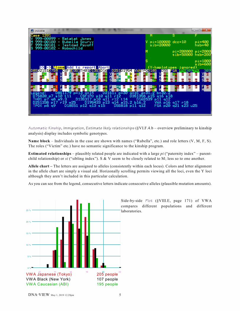
VW A Japanese (Tokyo) 205 people
VW A Black (New York) 107 people
VW A Caucasian (ABI) 195 people
Automatic Kinship, Immigration, Estimate likely relationships (§VI.F.4.b – overview preliminary to kinship
analysis) display includes symbolic genotypes.
Name block – Individuals in the case are shown with names (“Rubella”, etc.) and role letters (V, M, F, S).
The roles (“Victim” etc.) have no semantic significance to the kinship program.
Estimated relationships – plausibly related people are indicated with a large pi (“paternity index” – parent-
child relationship) or si (“sibling index”). S & V seem to be closely related to M; less so to one another.
Allele chart – The letters are assigned to alleles (consistently within each locus). Colors and letter alignment
in the allele chart are simply a visual aid. Horizonally scrolling permits viewing all the loci, even the Y loci
although they aren’t included in this particular calculation.
As you can see from the legend, consecutive letters indicate consecutive alleles (plausible mutation amounts).
Side-by-side Plot (§VIII.E, page 171) of VWA
compares different populations and different
laboratories.
DNA@VIEW May 1, 2019 12:29pm 5
DNA·VIEW®
DNA Identification Analysis Programs
USER’S MANUAL
Table of contents — overview
Message to users.. . . . . . . . . . . . . . . . . . . . . . . . . . . . . . . . . . . . . . . . . . . . . . . . . . . . . . . . . . . . . . . . . . . . 3
Detailed table of contents. . . . . . . . . . . . . . . . . . . . . . . . . . . . . . . . . . . . . . . . . . . . . . . . . . . . . . . . . . . . . . 7
List of Figures. . . . . . . . . . . . . . . . . . . . . . . . . . . . . . . . . . . . . . . . . . . . . . . . . . . . . . . . . . . . . . . . . . . . . 14
I GENERAL INFORMATION. . . . . . . . . . . . . . . . . . . . . . . . . . . . . . . . . . . . . . . . . . . . . . . . . . . . . . . . 17
II OPERATIONAL PROCEDURE.. . . . . . . . . . . . . . . . . . . . . . . . . . . . . . . . . . . . . . . . . . . . . . . . . . . . 29
III TUTORIAL – VARIOUS OPERATIONS.. . . . . . . . . . . . . . . . . . . . . . . . . . . . . . . . . . . . . . . . . . . . 33
IV TUTORIAL – CASEWORK. . . . . . . . . . . . . . . . . . . . . . . . . . . . . . . . . . . . . . . . . . . . . . . . . . . . . . . . 35
V CASEWORK ROUTINE. . . . . . . . . . . . . . . . . . . . . . . . . . . . . . . . . . . . . . . . . . . . . . . . . . . . . . . . . . 41
V.B Paternity Case V.C Case Options V.D Crime Case V.G DNA odds V.J Worklist etc.
VI KINSHIP. . . . . . . . . . . . . . . . . . . . . . . . . . . . . . . . . . . . . . . . . . . . . . . . . . . . . . . . . . . . . . . . . . . . . . 99
VII DISASTER ANALYSIS.. . . . . . . . . . . . . . . . . . . . . . . . . . . . . . . . . . . . . . . . . . . . . . . . . . . . . . . . 143
VIII POPULATIONS. . . . . . . . . . . . . . . . . . . . . . . . . . . . . . . . . . . . . . . . . . . . . . . . . . . . . . . . . . . . . . 157
IX MISCELLANEOUS OPERATIONS.. . . . . . . . . . . . . . . . . . . . . . . . . . . . . . . . . . . . . . . . . . . . . . . 195
X IMPORT/EXPORT. . . . . . . . . . . . . . . . . . . . . . . . . . . . . . . . . . . . . . . . . . . . . . . . . . . . . . . . . . . . . . 225
XI PROGRAM MAINTENANCE. . . . . . . . . . . . . . . . . . . . . . . . . . . . . . . . . . . . . . . . . . . . . . . . . . . . 251
XII EVALUATION OF EVIDENCE. . . . . . . . . . . . . . . . . . . . . . . . . . . . . . . . . . . . . . . . . . . . . . . . . . 261
XIII ALGORITHMS. . . . . . . . . . . . . . . . . . . . . . . . . . . . . . . . . . . . . . . . . . . . . . . . . . . . . . . . . . . . . . . 275
XIV USE OF THE KEYBOARD AND MOUSE.. . . . . . . . . . . . . . . . . . . . . . . . . . . . . . . . . . . . . . . . 287
XV APPENDIX — INSTALLATION AND UPDATE. . . . . . . . . . . . . . . . . . . . . . . . . . . . . . . . . . . . 295
XVI APPENDIX — REFERENCE TABLES. . . . . . . . . . . . . . . . . . . . . . . . . . . . . . . . . . . . . . . . . . . 311
XVI.B.4 BIBLIOGRAPHY. . . . . . . . . . . . . . . . . . . . . . . . . . . . . . . . . . . . . . . . . . . . . . . . . . . . . . . . . 316
Index. . . . . . . . . . . . . . . . . . . . . . . . . . . . . . . . . . . . . . . . . . . . . . . . . . . . . . . . . . . . . . . . . . . . . . . . . 320
DNA@VIEW May 1, 2019 12:29pm 6
Table of Contents
I. GENERAL INFORMATION. . . . . . . . . . . . . . . . . . . . . . . . . . . . . . . . . . . . . . . . . . . . . . . . . . . . . . . . 17
I.A. What is DNA·VIEW?. . . . . . . . . . . . . . . . . . . . . . . . . . . . . . . . . . . . . . . . . . . . . . . . . . . . . . 17
I.A.1. Software (17); I.A.2. Hardware (17)
I.B. Start Up. . . . . . . . . . . . . . . . . . . . . . . . . . . . . . . . . . . . . . . . . . . . . . . . . . . . . . . . . . . . . . . . . 17
I.C. Learning DNA·VIEW. . . . . . . . . . . . . . . . . . . . . . . . . . . . . . . . . . . . . . . . . . . . . . . . . . . . . . 18
I.C.1. Manual and release note (18); I.C.2. Program conventions (20); I.C.3. Telephone and
fax assistance (20); I.C.4. Select program option (20)
I.D. To Exit. . . . . . . . . . . . . . . . . . . . . . . . . . . . . . . . . . . . . . . . . . . . . . . . . . . . . . . . . . . . . . . . . 21
I.D.1. From a command (21); I.D.2. From graphics mode (21); I.D.3. From “special editing
mode” (21); I.D.4. From tools (21); I.D.5. To Windows (21); I.D.6. (Avoiding) program
delays (21)
I.E. The world of DNAAVIEW. . . . . . . . . . . . . . . . . . . . . . . . . . . . . . . . . . . . . . . . . . . . . . . . . . . 22
I.E.1. Data structures (22); I.E.2. Casework Analysis (24); I.E.3. Disaster Screening (25);
I.E.4. Single-profile or manual crime stain analysis (25); I.E.5. Prototype Kinship (26);
I.E.6. Database analysis (26); I.E.7. Reports in DNAAVIEW (26); I.E.8. Where to Find It
— Sub-menus (27); I.E.9. Where to Find It — Guide to DNA·VIEW (28)
II. OPERATIONAL PROCEDURE. . . . . . . . . . . . . . . . . . . . . . . . . . . . . . . . . . . . . . . . . . . . . . . . . . . . . 29
II.A. Outline of Operations.. . . . . . . . . . . . . . . . . . . . . . . . . . . . . . . . . . . . . . . . . . . . . . . . . . . . . 29
II.A.1. Routine for casework – very efficient method (29); II.A.2. Routine for casework –
second best method (29); II.A.3. Occasional operations (30)
II.B. Preliminaries — details. . . . . . . . . . . . . . . . . . . . . . . . . . . . . . . . . . . . . . . . . . . . . . . . . . . . 31
II.B.1. List of loci (31); II.B.2. List of races (31); II.B.3. Default data base (31); II.B.4.
List of readers (31); II.B.5. Define Quality Controls (31); II.B.6. Miscellaneous options III.
TUTORIAL — VARIOUS OPERATIONS. . . . . . . . . . . . . . . . . . . . . . . . . . . . . . . . . . 31
III.A. Quick installation. . . . . . . . . . . . . . . . . . . . . . . . . . . . . . . . . . . . . . . . . . . . . . . . . . . . . . . . 33
III.B. First execution of DNA·VIEW. . . . . . . . . . . . . . . . . . . . . . . . . . . . . . . . . . . . . . . . . . . . . . 33
III.C. Practice session with (stand-alone) Kinship.. . . . . . . . . . . . . . . . . . . . . . . . . . . . . . . . . . . 33
III.D. Finished!. . . . . . . . . . . . . . . . . . . . . . . . . . . . . . . . . . . . . . . . . . . . . . . . . . . . . . . . . . . . . . . 34
IV. TUTORIAL — CASEWORK. . . . . . . . . . . . . . . . . . . . . . . . . . . . . . . . . . . . . . . . . . . . . . . . . . . . . . 34
IV.A. Paternity and Kinship Casework. . . . . . . . . . . . . . . . . . . . . . . . . . . . . . . . . . . . . . . . . . . . 35
IV.A.1. Preview (35); IV.A.2. Sample case (35)
IV.B. Fast, typical method. . . . . . . . . . . . . . . . . . . . . . . . . . . . . . . . . . . . . . . . . . . . . . . . . . . . . . 35
IV.B.1. Import the data (36); IV.B.2. Compute paternity indices (36)
IV.C. Practice (automatic) Kinship Case. . . . . . . . . . . . . . . . . . . . . . . . . . . . . . . . . . . . . . . . . . . 36
IV.D. Manual methods. . . . . . . . . . . . . . . . . . . . . . . . . . . . . . . . . . . . . . . . . . . . . . . . . . . . . . . . . 37
IV.D.1. Practice session – modify case definition (38); IV.D.2. Practice session – create
empty case #14 (38); IV.D.3. Practice session – modify a roster (38); IV.D.4. Practice
session – modify DNA data (39)
IV.E. Crime stain practice. . . . . . . . . . . . . . . . . . . . . . . . . . . . . . . . . . . . . . . . . . . . . . . . . . . . . . 39
IV.E.1. profile computation – DNA odds (39)
IV.F. Some maintenance operations. . . . . . . . . . . . . . . . . . . . . . . . . . . . . . . . . . . . . . . . . . . . . . . 39
V. CASEWORK ROUTINE. . . . . . . . . . . . . . . . . . . . . . . . . . . . . . . . . . . . . . . . . . . . . . . . . . . . . . . . . . . 40
V.A. Open Case. . . . . . . . . . . . . . . . . . . . . . . . . . . . . . . . . . . . . . . . . . . . . . . . . . . . . . . . . . . . . 41
V.B. Paternity/Automatic Kinship Case. . . . . . . . . . . . . . . . . . . . . . . . . . . . . . . . . . . . . . . . . . . . 41
DNA@VIEW May 1, 2019 12:29pm 7
V.B.1. What is a Case? (41); V.B.2. Operation of the Case commands (41); V.B.3. add role
(42); V.B.4. batch run, batch select (43); V.B.5. calculate avuncular (44); V.B.6. calculate
trio/duo (45); V.B.7. calculate paternity/maternity (45); V.B.8. calculate family trio (47);
V.B.9. compute one locus (paternity analysis detail) (49); V.B.10. delete case (49); V.B.11.
edit case comment (50); V.B.12. edit people (50); V.B.13. edit race list (50); V.B.14.
export case (50); V.B.15. immigration/kinship (51); V.B.16. language is [paternity |
maternity | crime | kinship] (51); V.B.17. list cases (52); V.B.18. Let PRIOR= (0#p#1)
(52); V.B.19. Let THETA= (0#è<1) (53); V.B.20. locus parameters (53); V.B.21. Name
tag style: NAME/DATE (53); V.B.22. Null allele frequency: AUTO/ASK (53); V.B.23.
(case) options (54); V.B.24. recap (54); V.B.25. Reorder loci (54); V.B.26. restrict data
(54); V.B.27. review/print report (55); V.B.28. select case (56); V.B.29. simulation (56);
V.B.30. parentage test examples (57)
V.C. (Case) options. . . . . . . . . . . . . . . . . . . . . . . . . . . . . . . . . . . . . . . . . . . . . . . . . . . . . . . . . . . 57
V.C.1. Where Case Options are (58); V.C.2. Changing Case Options (58); V.C.3. Mutation
Case Options (58); V.C.4. Allele probability Case Options (58); V.C.5. Reports and filing
Case Options (59); V.C.6. Calculation Case Options (other than allele probability) (61)
V.D. Automatic mixture and Manual mixed stain. . . . . . . . . . . . . . . . . . . . . . . . . . . . . . . . . . . . 63
V.D.1. Purpose (65); V.D.2. Overview (65); V.D.3. Mixture ("LR") calculator operational
details (65); V.D.4. Master calculation screen for a scenario (66); V.D.5. Mixture
computation screen for one locus (68); V.D.6. Hints and techniques (70); V.D.7. Comments
(74); V.D.8. Forensic Calculation Logic (75); V.D.9. Mixture test suite (76)
V.E. Mixture Explorer (experimental). . . . . . . . . . . . . . . . . . . . . . . . . . . . . . . . . . . . . . . . . . . . . 76
V.E.1. Define search parameters (77); V.E.2. Exploring a mixture (77); V.E.3.
Understanding the results (77)
V.F. Mixture Solution – “continuous model” (experimental). . . . . . . . . . . . . . . . . . . . . . . . . . . 78
V.F.1. Expert system (80); V.F.2. Caveat (80); V.F.3. Operation of the continuous model
(81)
V.G. DNA Odds.. . . . . . . . . . . . . . . . . . . . . . . . . . . . . . . . . . . . . . . . . . . . . . . . . . . . . . . . . . . . . 81
V.G.1. Operation and capability (84); V.G.2. Action keys and menus (84); V.G.3.
“Modalities” of computation – various NRC II options (85)
V.H. Y-haplotype matching LR. . . . . . . . . . . . . . . . . . . . . . . . . . . . . . . . . . . . . . . . . . . . . . . . . . 86
V.H.1. Y-haplotype calculations (87); V.H.2. Operation (87)
V.I. DNA Exclusion. . . . . . . . . . . . . . . . . . . . . . . . . . . . . . . . . . . . . . . . . . . . . . . . . . . . . . . . . . . 87
V.I.1. Discussion of the “exclusion” statistic (89); V.I.2. Operation (89)
V.J. Worklist. . . . . . . . . . . . . . . . . . . . . . . . . . . . . . . . . . . . . . . . . . . . . . . . . . . . . . . . . . . . . . . . 90
V.J.1. Choose a worklist (92); V.J.2. Create a worklist (92); V.J.3. Enter or edit the roster
(93); V.J.4. Done with roster definition (94)
V.K. The File menu. . . . . . . . . . . . . . . . . . . . . . . . . . . . . . . . . . . . . . . . . . . . . . . . . . . . . . . . . . . 95
V.K.1. Print (96); V.K.2. Save As (96); V.K.3. Show report (96)
V.L. DNA Profiles. . . . . . . . . . . . . . . . . . . . . . . . . . . . . . . . . . . . . . . . . . . . . . . . . . . . . . . . . . . . 96
V.L.1. Operation (97); V.L.2. Comment (97)
VI. KINSHIP. . . . . . . . . . . . . . . . . . . . . . . . . . . . . . . . . . . . . . . . . . . . . . . . . . . . . . . . . . . . . . . . . . . . . . . 97
VI.A. Conceptual Overview. . . . . . . . . . . . . . . . . . . . . . . . . . . . . . . . . . . . . . . . . . . . . . . . . . . . . 99
VI.B. Kinship facilities in DNA·VIEW. . . . . . . . . . . . . . . . . . . . . . . . . . . . . . . . . . . . . . . . . . . . 99
VI.B.1. Two versions of Kinship (100); VI.B.2. Limitations (100)
VI.C. The Kinship notation. . . . . . . . . . . . . . . . . . . . . . . . . . . . . . . . . . . . . . . . . . . . . . . . . . . . 100
VI.C.1. Kinship semantic concepts (101); VI.C.2. Kinship syntax (101); VI.C.3. How to
learn the Kinship Notation (101); VI.C.4. Kinship Semantics, clarification, and examples
(103); VI.C.5. One hypothesis (105); VI.C.6. Prior probability (106)
VI.D. Multiple hypotheses in Kinship and Immigration/Kinship. . . . . . . . . . . . . . . . . . . . . . . . 106
DNA@VIEW May 1, 2019 12:29pm 8
VI.D.1. Multiple hypothesis syntax (107); VI.D.2. Multiple hypothesis result (107)
VI.E. Automatic Version of Kinship – Overview.. . . . . . . . . . . . . . . . . . . . . . . . . . . . . . . . . . . 107
VI.E.1. Preliminary (109)
VI.F. Immigration/kinship – operations . . . . . . . . . . . . . . . . . . . . . . . . . . . . . . . . . . . . . . . . . . 109
VI.F.1. Type in (or edit) scenario (110); VI.F.2. Calculate & report LRs, all races (111);
VI.F.3. Calculate LRs (current race) (113); VI.F.4. Estimating races and relationships (115);
VI.F.5. Y-haplotypes (115); VI.F.6. Bayesian options – prior and posterior probabilities
(117); VI.F.7. Detailed control and analysis of the calculation (119); VI.F.8.
Immigration/kinship – Kinship validation/consultation (120)
VI.G. Kinship Simulations. . . . . . . . . . . . . . . . . . . . . . . . . . . . . . . . . . . . . . . . . . . . . . . . . . . . . 123
VI.G.1. Purposes (124); VI.G.2. Outline of simulating (124); VI.G.3. Rules for simulation
(124); VI.G.4. Simulation Operation (124); VI.G.5. Simulation Summary (125); VI.G.6.
Saving simulation scenarios (127)
VI.H. The Prototype Kinship command (stand-alone Kinship program). . . . . . . . . . . . . . . . . . 132
VI.I. Kinship cases. . . . . . . . . . . . . . . . . . . . . . . . . . . . . . . . . . . . . . . . . . . . . . . . . . . . . . . . . . . 133
VI.J. Overview of using Prototype Kinship. . . . . . . . . . . . . . . . . . . . . . . . . . . . . . . . . . . . . . . 133
VI.J.1. a new problem (134); VI.J.2. a modified problem (134)
VI.K. Using the Prototype Kinship Command. . . . . . . . . . . . . . . . . . . . . . . . . . . . . . . . . . . . . . 134
VI.K.1. Define the relationships (135); VI.K.2. Set option toggles (135); VI.K.3. Find
formula for locus (135); VI.K.4. Algebraically simplify formula (for amusement only)
(136); VI.K.5. Evaluate formula (137); VI.K.6. Display pedigree/locus (137); VI.K.7. Save
the pedigree/locus in a complete case (138); VI.K.8. Display case summary (138); VI.K.9.
Run test cases; check program (138); VI.K.10. File or fetch complete case (138); VI.K.11.
Calculate additional loci (if any) (138); VI.K.12. Revising a complete case (139); VI.K.13.
Print report (139)
VI.L. Special situations. . . . . . . . . . . . . . . . . . . . . . . . . . . . . . . . . . . . . . . . . . . . . . . . . . . . . . . 140
VI.L.1. Twins (141); VI.L.2. Missing persons (141); VI.L.3. Indirect Exclusion (142)
VII. DISASTER ANALYSIS. . . . . . . . . . . . . . . . . . . . . . . . . . . . . . . . . . . . . . . . . . . . . . . . . . . . . . . . . 142
VII.A. Overview.. . . . . . . . . . . . . . . . . . . . . . . . . . . . . . . . . . . . . . . . . . . . . . . . . . . . . . . . . . . . 143
VII.A.1. There are four major steps to the analysis: (143); VII.A.2. Additional –
method+tool to establish reference allele frequencies (143); VII.A.2. Additional –
method+tool to establish reference allele frequencies (144)
VII.B. Import DNA profiles . . . . . . . . . . . . . . . . . . . . . . . . . . . . . . . . . . . . . . . . . . . . . . . . . . . 144
VII.B.1. Overview (144); VII.B.2. Import profiles (144)
VII.C. Collapse Victim Profiles. . . . . . . . . . . . . . . . . . . . . . . . . . . . . . . . . . . . . . . . . . . . . . . . . 145
VII.C.1. Description (145); VII.C.2. Operation (145)
VII.D. Screening. . . . . . . . . . . . . . . . . . . . . . . . . . . . . . . . . . . . . . . . . . . . . . . . . . . . . . . . . . . . 146
VII.D.1. Overview (148); VII.D.2. Result (148); VII.D.3. Operation (148)
VII.E. Screening summary. . . . . . . . . . . . . . . . . . . . . . . . . . . . . . . . . . . . . . . . . . . . . . . . . . . . . 149
VII.F. Test Candidate Relationship using Kinship. . . . . . . . . . . . . . . . . . . . . . . . . . . . . . . . . . . 153
VII.F.1. Kinship steps (153); VII.F.2. Technical comments about evaluating identifications
(153); VII.F.3. More hints (154)
VII.G. Assign Race to Worklist. . . . . . . . . . . . . . . . . . . . . . . . . . . . . . . . . . . . . . . . . . . . . . . . . 154
VIII. POPULATIONS.. . . . . . . . . . . . . . . . . . . . . . . . . . . . . . . . . . . . . . . . . . . . . . . . . . . . . . . . . . . . . . 157
VIII.A. Population databases. . . . . . . . . . . . . . . . . . . . . . . . . . . . . . . . . . . . . . . . . . . . . . . . . . . 157
VIII.B. Population commands. . . . . . . . . . . . . . . . . . . . . . . . . . . . . . . . . . . . . . . . . . . . . . . . . . 157
VIII.C. Database.. . . . . . . . . . . . . . . . . . . . . . . . . . . . . . . . . . . . . . . . . . . . . . . . . . . . . . . . . . . . 158
VIII.C.1. What a database is (158); VIII.C.2. Default databases (159); VIII.C.3. Ways to
make a database (159); VIII.C.4. Building and maintaining allele population data
DNA@VIEW May 1, 2019 12:29pm 9
(“database”) in DNA@VIEW (162); VIII.C.5. Compile a new database from DNA AVIEW
data (165); VIII.C.6. Side effects (166); VIII.C.7. Updating (166); VIII.C.8. Review
exception report (167); VIII.C.9. Delete or rename (167); VIII.C.10. Combine (167);
VIII.C.11. List of homozygotes (168); VIII.C.12. Edit or type in a database (168);
VIII.C.13. Document sample frequencies etc. tables (169); VIII.C.14. Print allele list,
frequencies (RFLP) (169)
VIII.D. Database statistics and information. . . . . . . . . . . . . . . . . . . . . . . . . . . . . . . . . . . . . . . . 170
VIII.D.1. Operation (170); VIII.D.2. Results (170)
VIII.E. Plot. . . . . . . . . . . . . . . . . . . . . . . . . . . . . . . . . . . . . . . . . . . . . . . . . . . . . . . . . . . . . . . . . 171
VIII.E.1. Operation (171); VIII.E.2. Experimental Plot features (172)
VIII.F. Y haplotypes in DNA@VIEW. . . . . . . . . . . . . . . . . . . . . . . . . . . . . . . . . . . . . . . . . . . . . 174
VIII.F.1. Y haplotype overview (174); VIII.F.2. Y Databases functions (175); VIII.F.3.
Install Y-haplotype databases from worklist (175); VIII.F.4. Rename, reorder, delete Y
databases (176); VIII.F.5. Y-haplotype database statistics (177)
VIII.G. Exact Tests for Independence. . . . . . . . . . . . . . . . . . . . . . . . . . . . . . . . . . . . . . . . . . . . 178
VIII.H. Hardy-Weinberg Exact Test; Independence of Loci. . . . . . . . . . . . . . . . . . . . . . . . . . . 179
VIII.H.1. Type in phenotype counts for a Hardy-Weinberg check (180); VIII.H.2. Monte
Carlo calculation (180); VIII.H.3. Ascii export, or import a triangle of phenotype counts
(181); VIII.H.4. Import columnar genotype data (181)
VIII.I. Database similarity test. . . . . . . . . . . . . . . . . . . . . . . . . . . . . . . . . . . . . . . . . . . . . . . . . . 186
VIII.I.1. Outline of use (186); VIII.I.2. Operation (186)
VIII.J. Allele report – rare and common alleles. . . . . . . . . . . . . . . . . . . . . . . . . . . . . . . . . . . . . 187
VIII.K. Mutation history.. . . . . . . . . . . . . . . . . . . . . . . . . . . . . . . . . . . . . . . . . . . . . . . . . . . . . . 189
VIII.K.1. Overview (189); VIII.K.2. Preliminaries for mutation analysis (189); VIII.K.3.
Mutation report (190)
VIII.L. Racial “Discrimination”. . . . . . . . . . . . . . . . . . . . . . . . . . . . . . . . . . . . . . . . . . . . . . . . . 192
VIII.M. Racial distances – compare many races.. . . . . . . . . . . . . . . . . . . . . . . . . . . . . . . . . . . . 192
VIII.M.1. Uses (192); VIII.M.2. Background (192); VIII.M.3. Operation (193)
VIII.N. Racial estimation. . . . . . . . . . . . . . . . . . . . . . . . . . . . . . . . . . . . . . . . . . . . . . . . . . . . . . 193
VIII.N.1. Initiate operation (193); VIII.N.2. Tentatively choose races to compare (193);
VIII.N.3. Consider racial mixtures? (194); VIII.N.4. Choose races to compare (194);
VIII.N.5. Result (194)
IX. MISCELLANEOUS OPERATIONS. . . . . . . . . . . . . . . . . . . . . . . . . . . . . . . . . . . . . . . . . . . . . . . . 195
IX.A. Maintenance. . . . . . . . . . . . . . . . . . . . . . . . . . . . . . . . . . . . . . . . . . . . . . . . . . . . . . . . . . . 195
IX.A.1. Locus parameters & preferences (195); IX.A.2. Locus report (195); IX.A.3. locus
list by chromosome (196); IX.A.4. Races (197); IX.A.5. Readers (197); IX.A.6. Worklist
configuration/formats (add or list) (197); IX.A.7. standard ladder/molecular weight marker
(report, add) (198); IX.A.8. Network preferences (for Paradox) (198); IX.A.9. document
Paradox table (198); IX.A.10. rebuild Paradox index (199); IX.A.11. report systemwide
switch/parameter settings (199); IX.A.12. record switch/parameter settings (199); IX.A.13.
compare switch/parameter settings (199); IX.A.14. rewrite (compress) files – conserve disk
space (200); IX.A.15. Password access to critical DNA@VIEW functions (200)
IX.B. Probe/locus maintenance. . . . . . . . . . . . . . . . . . . . . . . . . . . . . . . . . . . . . . . . . . . . . . . . . 201
IX.B.1. Locus maintenance (201); IX.B.2. Locus maintenance screen (201); IX.B.3. PCR
parameters (203); IX.B.4. Locus parameters (mutation, rare allele rates) (204); IX.B.5.
Additional locus topics (205); IX.B.6. Locus status and Restriction enzymes (206); IX.B.7.
Multiplexes (207)
IX.C. Worklist Sizes.. . . . . . . . . . . . . . . . . . . . . . . . . . . . . . . . . . . . . . . . . . . . . . . . . . . . . . . . . 207
IX.D. Statistics. . . . . . . . . . . . . . . . . . . . . . . . . . . . . . . . . . . . . . . . . . . . . . . . . . . . . . . . . . . . . . 208
IX.D.1. Intra-assay versus Inter-assay (208)
DNA@VIEW May 1, 2019 12:29pm 10
IX.E. Browse. . . . . . . . . . . . . . . . . . . . . . . . . . . . . . . . . . . . . . . . . . . . . . . . . . . . . . . . . . . . . . . 208
IX.E.1. Change name or comment (209); IX.E.2. Lane deletion (209); IX.E.3. Read
deletion (210); IX.E.4. Worklist, Configuration, and Standards ladder deletion (210)
IX.F. Options. . . . . . . . . . . . . . . . . . . . . . . . . . . . . . . . . . . . . . . . . . . . . . . . . . . . . . . . . . . . . . . 211
IX.F.1. Box drawing characters (211); IX.F.2. Case # format: 09/00123 (211); IX.F.3.
Command menu style: FLAT/2 levels (211); IX.F.4. Compare report style (212); IX.F.5.
Convert accession codes: (none) / WTC / Katrina (212); IX.F.6. Date order: 3/18/2008
(212); IX.F.7. Decimal marker: . (dot) (212); IX.F.8. DNA@VIEW character translation
(213); IX.F.9. DNA@VIEW Printer (213); IX.F.10. DNA@VIEW Printer port (213); IX.F.11.
DNA @VIEW report title line (214); IX.F.12. DNAAVIEW report includes: [Version,
Workstation] (214); IX.F.13. DNA@VIEW report epilogue (214); IX.F.14. Default date?
(214); IX.F.15. Graphics detail scaling (214); IX.F.16. Interpolation parameters (214);
IX.F.17. Keyboard (214); IX.F.18. Language (214); IX.F.19. Locus name style like:
D16S539 STR (214); IX.F.20. Locus parameters (215); IX.F.21. Message display time
(215); IX.F.22. Minimum frequency parameters (215); IX.F.23. Name tag style:
NAME/DATE (215); IX.F.24. Numlock on/off (215); IX.F.25. Off-ladder allele policy:
DISCARD/RARE (215); IX.F.26. Options from "Case" (215); IX.F.27. PCR allele binning?
NO/YES (215); IX.F.28. PCR notation style (215); IX.F.29. page format (215); IX.F.30.
Paradox directory (216); IX.F.31. PATER character translation (217); IX.F.32. PATER
signature line (217); IX.F.33. PATER Logo (217); IX.F.34. Plot line thickness (217);
IX.F.35. RFLP: disabled (217); IX.F.36. Window style (217)
IX.G. Profile Data. . . . . . . . . . . . . . . . . . . . . . . . . . . . . . . . . . . . . . . . . . . . . . . . . . . . . . . . . . . 218
IX.H. Compare. . . . . . . . . . . . . . . . . . . . . . . . . . . . . . . . . . . . . . . . . . . . . . . . . . . . . . . . . . . . . . 218
IX.I. Directory. . . . . . . . . . . . . . . . . . . . . . . . . . . . . . . . . . . . . . . . . . . . . . . . . . . . . . . . . . . . . . 219
IX.J. Quality Control. . . . . . . . . . . . . . . . . . . . . . . . . . . . . . . . . . . . . . . . . . . . . . . . . . . . . . . . . 220
IX.J.1. add control (220); IX.J.2. disenroll control (220); IX.J.3. edit stats (220); IX.J.4.
list (221); IX.J.5. print (222); IX.J.6. range report (222); IX.J.7. recompute (222); IX.J.8.
show details (222)
X. IMPORT/EXPORT. . . . . . . . . . . . . . . . . . . . . . . . . . . . . . . . . . . . . . . . . . . . . . . . . . . . . . . . . . . . . . 225
X.A. Import/Export – import DNA profile data. . . . . . . . . . . . . . . . . . . . . . . . . . . . . . . . . . . . . 226
X.A.1. Importing steps – preliminary (226); X.A.2. Importing steps – in DNAAVIEW (226);
X.A.3. File formats (226); X.A.4. Genotyper import file format (230); X.A.5. GeneMapper
import (231); X.A.6. Hitachi STRCALL Import (232); X.A.7. File format details (233);
X.A.8. Defining the roster (235); X.A.9. DNA@VIEW and Osiris (236)
X.B. Import/Export – databases. . . . . . . . . . . . . . . . . . . . . . . . . . . . . . . . . . . . . . . . . . . . . . . . 236
X.B.1. Allele frequency (or count) population data import (240); X.B.2. Genotype table
of population sample. (Pair of columns=genotype for a locus) (243)
X.C. . . . . . . . . . . . . . . . . . . . . . . . . . . . . . . . . . . . . . . . . . . . . . . . . . . . . . . . . . . . . . . . . . . . . . . 245
X.C.1. DNA@VIEW Frequency Database Import (transfer between users) (246); X.C.2.
Export DNA@VIEW databases (transfer between users) (246)
X.D. Import/Export – GeneScan & Pharmacia.. . . . . . . . . . . . . . . . . . . . . . . . . . . . . . . . . . . . . 247
X.E. Import/Export – miscellaneous options. . . . . . . . . . . . . . . . . . . . . . . . . . . . . . . . . . . . . . . 247
X.E.1. List and search database profiles (247); X.E.2. LIMS import of case & person
definitions (247); X.E.3. Case and accession data import (250)
X.F. CODIS: export size data in CMF format. . . . . . . . . . . . . . . . . . . . . . . . . . . . . . . . . . . . . . 250
X.G. Integration of DNA•VIEW within LIMS system.. . . . . . . . . . . . . . . . . . . . . . . . . . . . . . . 250
XI. PROGRAM VALIDATION & MAINTENANCE. . . . . . . . . . . . . . . . . . . . . . . . . . . . . . . . . . . . . . 251
XI.A. Program Validation. . . . . . . . . . . . . . . . . . . . . . . . . . . . . . . . . . . . . . . . . . . . . . . . . . . . . 251
DNA@VIEW May 1, 2019 12:29pm 11
XI.A.1. Test suites in DNA@VIEW (251); XI.A.2. Facilities for documenting DNA@VIEW
settings (251); XI.A.3. Protocol for casework validation (252); XI.A.4. Database validation
(252)
XI.B. Update. . . . . . . . . . . . . . . . . . . . . . . . . . . . . . . . . . . . . . . . . . . . . . . . . . . . . . . . . . . . . . . 253
XI.C. Program Errors. . . . . . . . . . . . . . . . . . . . . . . . . . . . . . . . . . . . . . . . . . . . . . . . . . . . . . . . . 253
XI.C.1. Wrong answers (253); XI.C.2. Fatal errors (253); XI.C.3. Network lock (253)
XI.D. DNA·VIEW Files.. . . . . . . . . . . . . . . . . . . . . . . . . . . . . . . . . . . . . . . . . . . . . . . . . . . . . . 254
XI.D.1. Data files (254); XI.D.2. Security, Backing up data (254); XI.D.3. Program files
(255)
XI.E. PATER or DEMO . . . . . . . . . . . . . . . . . . . . . . . . . . . . . . . . . . . . . . . . . . . . . . . . . . . . . . 255
XI.F. tools (requires supervision). . . . . . . . . . . . . . . . . . . . . . . . . . . . . . . . . . . . . . . . . . . . . . . . 256
XI.F.1. Reindex (257); XI.F.2. Push_Me (257); XI.F.3. Repair (258)
XI.G. Repair Paradox problems. . . . . . . . . . . . . . . . . . . . . . . . . . . . . . . . . . . . . . . . . . . . . . . . . 259
XI.G.1. Reasons for trying Repair include (259); XI.G.2. Repair operation. (259)
XII. EVALUATION OF EVIDENCE. . . . . . . . . . . . . . . . . . . . . . . . . . . . . . . . . . . . . . . . . . . . . . . . . . 260
XII.A. Concepts. . . . . . . . . . . . . . . . . . . . . . . . . . . . . . . . . . . . . . . . . . . . . . . . . . . . . . . . . . . . . 261
XII.A.1. Scientific Decision Making; a Primer (261); XII.A.2. The Likelihood Ratio (261);
XII.A.3. Essen-Möller’s equation (264); XII.A.4. Likelihood ratios in DNA@VIEW (264)
XII.B. PI. . . . . . . . . . . . . . . . . . . . . . . . . . . . . . . . . . . . . . . . . . . . . . . . . . . . . . . . . . . . . . . . . . . 265
XII.B.1. Using PI (265); XII.B.2. PI program examples (265); XII.B.3. PI control panel
discussion (266)
XII.C. Paternity Index Discussion. . . . . . . . . . . . . . . . . . . . . . . . . . . . . . . . . . . . . . . . . . . . . . . 266
XII.D. Explaining the result. . . . . . . . . . . . . . . . . . . . . . . . . . . . . . . . . . . . . . . . . . . . . . . . . . . 269
XII.E. Comparing three or more hypotheses. . . . . . . . . . . . . . . . . . . . . . . . . . . . . . . . . . . . . . . 269
XII.E.1. A 3-hypothesis case (271)
XII.F. Special situations. . . . . . . . . . . . . . . . . . . . . . . . . . . . . . . . . . . . . . . . . . . . . . . . . . . . . . . 271
XII.F.1. Motherless cases (273); XII.F.2. Homozygotes versus 1-banded patterns (273)
XIII. ALGORITHMS. . . . . . . . . . . . . . . . . . . . . . . . . . . . . . . . . . . . . . . . . . . . . . . . . . . . . . . . . . . . . . . 275
XIII.A. Probability computations. . . . . . . . . . . . . . . . . . . . . . . . . . . . . . . . . . . . . . . . . . . . . . . . 275
XIII.A.1. Match window probability (275)
XIII.B. Computation of Paternity Index. . . . . . . . . . . . . . . . . . . . . . . . . . . . . . . . . . . . . . . . . . . 275
XIII.B.1. Basic approach (window style) (278); XIII.B.2. Matching patterns (278);
XIII.B.3. Paternal alleles (278); XIII.B.4. Motherless case (278); XIII.B.5. Homozygosity
vs. single-allele (279); XIII.B.6. Mutation calculation (279)
XIII.C. Mutation calculations. . . . . . . . . . . . . . . . . . . . . . . . . . . . . . . . . . . . . . . . . . . . . . . . . . . 281
XIII.C.1. Principles of mutation calculations (281); XIII.C.2. Mendelian model (281);
XIII.C.3. STR mutation model (282); XIII.C.4. The simple or AABB mutation model (for
RFLP) (282)
XIII.D. Null Alleles in Kinship. . . . . . . . . . . . . . . . . . . . . . . . . . . . . . . . . . . . . . . . . . . . . . . . . 284
XIII.E. Mutation and kinship. . . . . . . . . . . . . . . . . . . . . . . . . . . . . . . . . . . . . . . . . . . . . . . . . . . 285
XIII.F. Averaging sizes together.. . . . . . . . . . . . . . . . . . . . . . . . . . . . . . . . . . . . . . . . . . . . . . . . 285
XIII.F.1. Several reads of a lane (285); XIII.F.2. Several lanes (286)
XIV. USE OF THE KEYBOARD AND MOUSE. . . . . . . . . . . . . . . . . . . . . . . . . . . . . . . . . . . . . . . . . 286
XIV.A. Answering prompts. . . . . . . . . . . . . . . . . . . . . . . . . . . . . . . . . . . . . . . . . . . . . . . . . . . . 287
XIV.A.1. Buttons (287); XIV.A.2. Selection from a list of choices (287); XIV.A.3.
Multiple selections (288); XIV.A.4. Numeric and text responses (288); XIV.A.5. Entering
probabilities (290); XIV.A.6. Yes/No prompts (291); XIV.A.7. Dates (291); XIV.A.8.
Mouse input methods (291); XIV.A.9. People (291); XIV.A.10. Case numbering (292)
DNA@VIEW May 1, 2019 12:29pm 12
XIV.B. Special Editing Screen. . . . . . . . . . . . . . . . . . . . . . . . . . . . . . . . . . . . . . . . . . . . . . . . . . 294
XV. APPENDIX — INSTALLATION AND UPDATE. . . . . . . . . . . . . . . . . . . . . . . . . . . . . . . . . . . . 295
XV.A. Installation. . . . . . . . . . . . . . . . . . . . . . . . . . . . . . . . . . . . . . . . . . . . . . . . . . . . . . . . . . . 295
XV.B. Preliminary for network installation. . . . . . . . . . . . . . . . . . . . . . . . . . . . . . . . . . . . . . . . 295
XV.B.1. For installation to a network server, (295)
XV.C. Begin installation. . . . . . . . . . . . . . . . . . . . . . . . . . . . . . . . . . . . . . . . . . . . . . . . . . . . . . 295
XV.C.1. Password (295); XV.C.2. Select Destination Location (295); XV.C.3. Select components
(295); XV.C.4. Select additional tasks (296); XV.C.5. First execution of DNA@VIEW (296);
XV.C.6. Install Pater (296)
XV.D. Networking. . . . . . . . . . . . . . . . . . . . . . . . . . . . . . . . . . . . . . . . . . . . . . . . . . . . . . . . . . . 297
XV.D.1. Turn on networking (297); XV.D.2. Icons (297); XV.D.3. How to print to a USB
printer (298); XV.D.4. Customizing the icons (298); XV.D.5. Start DNA·VIEW (300);
XV.D.6. Graphics checkout (300); XV.D.7. Mouse checkout. (300); XV.D.8. De-
installing a DNA·VIEW System Update (300); XV.D.9. Installing Frequency databases
(300); XV.D.10. Installation — Check (301); XV.D.11. Printing from DNAAVIEW (in
Windows) (301)
XV.E. Running DNA@VIEW under Windows. . . . . . . . . . . . . . . . . . . . . . . . . . . . . . . . . . . . . . 302
XV.E.1. Startup (303); XV.E.2. Hardware security key (303); XV.E.3. Startup with
graphics (303); XV.E.4. Annoying message (303)
XV.F. DNA·VIEW and Networks. . . . . . . . . . . . . . . . . . . . . . . . . . . . . . . . . . . . . . . . . . . . . . . 303
XV.F.1. Installation of DNA@VIEW to the server (305); XV.F.2. Install to other
workstations (305); XV.F.3. File sharing among workstations (306); XV.F.4. Cloned
DNA@VIEW on a network (306); XV.F.5. Personalized network configuration (307)
XV.G. Moving DNA·VIEW. . . . . . . . . . . . . . . . . . . . . . . . . . . . . . . . . . . . . . . . . . . . . . . . . . . 307
XV.H. Create a test platform for a new DNA@VIEW version.. . . . . . . . . . . . . . . . . . . . . . . . . . 308
XV.H.1. Installation (308); XV.H.2. Using and testing (308); XV.H.3. Updating to the new
version (308)
XV.I. Web conference. . . . . . . . . . . . . . . . . . . . . . . . . . . . . . . . . . . . . . . . . . . . . . . . . . . . . . . . 308
XV.I.1. What is a web conference? (309); XV.I.2. How to join (309)
XVI. APPENDIX — REFERENCE TABLES. . . . . . . . . . . . . . . . . . . . . . . . . . . . . . . . . . . . . . . . . . . . 309
XVI.A. Role letter/name assignments. . . . . . . . . . . . . . . . . . . . . . . . . . . . . . . . . . . . . . . . . . . . 311
XVI.A.1. Role name semantics (311); XVI.A.2. Official locus list (311); XVI.A.3. Official
enzyme and pseudo-enzyme list (313)
XVI.B. Paradox tables. . . . . . . . . . . . . . . . . . . . . . . . . . . . . . . . . . . . . . . . . . . . . . . . . . . . . . . . 315
XVI.B.1. PDIR (315); XVI.B.2. CDIR (315); XVI.B.3. DNAAPPRO and Post to a text file
(315); XVI.B.4. STRDATA (316)
XVII. BIBLIOGRAPHY. . . . . . . . . . . . . . . . . . . . . . . . . . . . . . . . . . . . . . . . . . . . . . . . . . . . . . . . . . . . . 317
(309)
DNA@VIEW May 1, 2019 12:29pm 13
List of Figures
Colorful display of symbolic genotype relationships. . . . . . . . . . . . . . . . . . . . . . . . . . . . . . . . . . . . . . . . . . 5
STR Plot comparing races and laboratories.. . . . . . . . . . . . . . . . . . . . . . . . . . . . . . . . . . . . . . . . . . . . . . . . 5
Figure 1 DNA@VIEW top level command menu. . . . . . . . . . . . . . . . . . . . . . . . . . . . . . . . . . . . . . . . . . . 18
Figure 2 DNA·VIEW top & second level menu commands.. . . . . . . . . . . . . . . . . . . . . . . . . . . . . . . . . . 19
Figure 3 Schematic workflow for casework. . . . . . . . . . . . . . . . . . . . . . . . . . . . . . . . . . . . . . . . . . . . . . . 29
Figure 5 Case nametag matrix and subcommand menu. . . . . . . . . . . . . . . . . . . . . . . . . . . . . . . . . . . . . . 41
Figure 6 Case menu options. . . . . . . . . . . . . . . . . . . . . . . . . . . . . . . . . . . . . . . . . . . . . . . . . . . . . . . . . . . 42
Figure 7 adding a second child. . . . . . . . . . . . . . . . . . . . . . . . . . . . . . . . . . . . . . . . . . . . . . . . . . . . . . . . . 43
Figure 8 batch select options. . . . . . . . . . . . . . . . . . . . . . . . . . . . . . . . . . . . . . . . . . . . . . . . . . . . . . . . . . 44
Figure 9 Calculate trio/duo panel. . . . . . . . . . . . . . . . . . . . . . . . . . . . . . . . . . . . . . . . . . . . . . . . . . . . . . . 45
Figure 10 Case report. . . . . . . . . . . . . . . . . . . . . . . . . . . . . . . . . . . . . . . . . . . . . . . . . . . . . . . . . . . . . . . . 47
Figure 11 compute one locus. . . . . . . . . . . . . . . . . . . . . . . . . . . . . . . . . . . . . . . . . . . . . . . . . . . . . . . . . . 49
Figure 14 Case list by case. . . . . . . . . . . . . . . . . . . . . . . . . . . . . . . . . . . . . . . . . . . . . . . . . . . . . . . . . . . . 53
Figure 15 The Recapitulation report. . . . . . . . . . . . . . . . . . . . . . . . . . . . . . . . . . . . . . . . . . . . . . . . . . . . . 54
Figure 16 restrict data selection screen. . . . . . . . . . . . . . . . . . . . . . . . . . . . . . . . . . . . . . . . . . . . . . . . . . . 55
Figure 18 Index of Case Options. . . . . . . . . . . . . . . . . . . . . . . . . . . . . . . . . . . . . . . . . . . . . . . . . . . . . . . 58
Figure 19 Formatted paternity report (“standard/LIMS”). . . . . . . . . . . . . . . . . . . . . . . . . . . . . . . . . . . . . 62
Figure 20 Define a mixture scenario. . . . . . . . . . . . . . . . . . . . . . . . . . . . . . . . . . . . . . . . . . . . . . . . . . . . . 67
Figure 21 Master calculation screen (“binary” mixture analysis). . . . . . . . . . . . . . . . . . . . . . . . . . . . . . . 68
Figure 24 DNA Odds screen. . . . . . . . . . . . . . . . . . . . . . . . . . . . . . . . . . . . . . . . . . . . . . . . . . . . . . . . . . 84
Figure 25 Y-haplotype matching LR screen. . . . . . . . . . . . . . . . . . . . . . . . . . . . . . . . . . . . . . . . . . . . . 87
Figure 26 DNA Exclusion screen. . . . . . . . . . . . . . . . . . . . . . . . . . . . . . . . . . . . . . . . . . . . . . . . . . . . . . . 90
Figure 30 Worklist exit menu. . . . . . . . . . . . . . . . . . . . . . . . . . . . . . . . . . . . . . . . . . . . . . . . . . . . . . . . . 95
Figure 31 printer “port” options. . . . . . . . . . . . . . . . . . . . . . . . . . . . . . . . . . . . . . . . . . . . . . . . . . . . . . . . 96
Figure 35 Kinship chapter index . . . . . . . . . . . . . . . . . . . . . . . . . . . . . . . . . . . . . . . . . . . . . . . . . . . . . . . 99
Figure 36 full sibling. . . . . . . . . . . . . . . . . . . . . . . . . . . . . . . . . . . . . . . . . . . . . . . . . . . . . . . . . . . . . . . 104
Figure 37 unrelated.. . . . . . . . . . . . . . . . . . . . . . . . . . . . . . . . . . . . . . . . . . . . . . . . . . . . . . . . . . . . . . . . 104
Figure 38 Immigration/Kinship options. . . . . . . . . . . . . . . . . . . . . . . . . . . . . . . . . . . . . . . . . . . . . . . . . 110
Figure 39 Immigration/Kinship options. . . . . . . . . . . . . . . . . . . . . . . . . . . . . . . . . . . . . . . . . . . . . . . . . 111
Figure 40 Table of symbolic genotypes. . . . . . . . . . . . . . . . . . . . . . . . . . . . . . . . . . . . . . . . . . . . . . . . . 112
Figure 41 Kinship LR’s, all races. . . . . . . . . . . . . . . . . . . . . . . . . . . . . . . . . . . . . . . . . . . . . . . . . . . . . . 113
Figure 42 Kinship "formatted report". . . . . . . . . . . . . . . . . . . . . . . . . . . . . . . . . . . . . . . . . . . . . . . . . . . 114
Figure 43 Kinship LR details. . . . . . . . . . . . . . . . . . . . . . . . . . . . . . . . . . . . . . . . . . . . . . . . . . . . . . . . . 115
Figure 44 estimated relationships. . . . . . . . . . . . . . . . . . . . . . . . . . . . . . . . . . . . . . . . . . . . . . . . . . . . . . 116
Figure 45 Customizing genotype display for page 5.. . . . . . . . . . . . . . . . . . . . . . . . . . . . . . . . . . . . . . . 116
Figure 46 Racial origin likelihoods. . . . . . . . . . . . . . . . . . . . . . . . . . . . . . . . . . . . . . . . . . . . . . . . . . . . 117
Figure 47 Y-haplotype matching LR. . . . . . . . . . . . . . . . . . . . . . . . . . . . . . . . . . . . . . . . . . . . . . . . . . . 118
Figure 52 parsing and kinship for one locus.. . . . . . . . . . . . . . . . . . . . . . . . . . . . . . . . . . . . . . . . . . . . . 120
Figure 53 genotype eyeball report. . . . . . . . . . . . . . . . . . . . . . . . . . . . . . . . . . . . . . . . . . . . . . . . . . . . . 121
Figure 54 probability expression. . . . . . . . . . . . . . . . . . . . . . . . . . . . . . . . . . . . . . . . . . . . . . . . . . . . . . 123
Figure 55 Kinship Simulation options and menu categories. . . . . . . . . . . . . . . . . . . . . . . . . . . . . . . . . 124
Figure 56 Incest pedigree. . . . . . . . . . . . . . . . . . . . . . . . . . . . . . . . . . . . . . . . . . . . . . . . . . . . . . . . . . . . 126
Figure 57 Paste saves typing.. . . . . . . . . . . . . . . . . . . . . . . . . . . . . . . . . . . . . . . . . . . . . . . . . . . . . . . . . 126
Figure 58 Simulation summary. . . . . . . . . . . . . . . . . . . . . . . . . . . . . . . . . . . . . . . . . . . . . . . . . . . . . . . 127
Figure 59 Incest LR distribution; Identifiler test of mother and child. . . . . . . . . . . . . . . . . . . . . . . . . . 128
Figure 60 Simulation record, NO details. . . . . . . . . . . . . . . . . . . . . . . . . . . . . . . . . . . . . . . . . . . . . . . . 130
Figure 61 Simulation record, BRIEF details (2 examples). . . . . . . . . . . . . . . . . . . . . . . . . . . . . . . . . . . 130
Figure 62 Simulation record, COMPLETE details. . . . . . . . . . . . . . . . . . . . . . . . . . . . . . . . . . . . . . . . . 131
DNA@VIEW May 1, 2019 12:29pm 14
Figure 63 Kinship options. . . . . . . . . . . . . . . . . . . . . . . . . . . . . . . . . . . . . . . . . . . . . . . . . . . . . . . . . . . 135
Figure 64 Deficiency case pedigree. . . . . . . . . . . . . . . . . . . . . . . . . . . . . . . . . . . . . . . . . . . . . . . . . . . . 135
Figure 65 Parsing output. . . . . . . . . . . . . . . . . . . . . . . . . . . . . . . . . . . . . . . . . . . . . . . . . . . . . . . . . . . . 136
Figure 66 Kinship case summary. . . . . . . . . . . . . . . . . . . . . . . . . . . . . . . . . . . . . . . . . . . . . . . . . . . . . . 140
Figure 68 Monozygotic vs. dizygotic twins. . . . . . . . . . . . . . . . . . . . . . . . . . . . . . . . . . . . . . . . . . . . . . 141
Figure 69 Missing person and corpse. . . . . . . . . . . . . . . . . . . . . . . . . . . . . . . . . . . . . . . . . . . . . . . . . . . 142
Figure 70 Missing person solution. . . . . . . . . . . . . . . . . . . . . . . . . . . . . . . . . . . . . . . . . . . . . . . . . . . . . 142
Figure 71 Screen reporting parameters – Likelihood ratio model. . . . . . . . . . . . . . . . . . . . . . . . . . . . . 150
Figure 73 Population commands. . . . . . . . . . . . . . . . . . . . . . . . . . . . . . . . . . . . . . . . . . . . . . . . . . . . . . 157
Figure 74 Database command options.. . . . . . . . . . . . . . . . . . . . . . . . . . . . . . . . . . . . . . . . . . . . . . . . . 158
Figure 80 Database printout. . . . . . . . . . . . . . . . . . . . . . . . . . . . . . . . . . . . . . . . . . . . . . . . . . . . . . . . . . 169
Figure 83 selecting parameters for a Plot. . . . . . . . . . . . . . . . . . . . . . . . . . . . . . . . . . . . . . . . . . . . . . . . 171
Figure 84 Installing Y-haplotype databases. . . . . . . . . . . . . . . . . . . . . . . . . . . . . . . . . . . . . . . . . . . . . . 176
Figure 85 Y-haplotype maintenance screen. . . . . . . . . . . . . . . . . . . . . . . . . . . . . . . . . . . . . . . . . . . . . . 176
Figure 86 Exact Test options. . . . . . . . . . . . . . . . . . . . . . . . . . . . . . . . . . . . . . . . . . . . . . . . . . . . . . . . . 179
Figure 87 HW exact test. . . . . . . . . . . . . . . . . . . . . . . . . . . . . . . . . . . . . . . . . . . . . . . . . . . . . . . . . . . . . 180
Figure 88 Genotype file format. . . . . . . . . . . . . . . . . . . . . . . . . . . . . . . . . . . . . . . . . . . . . . . . . . . . . . . 181
Figure 89 Subpopulation and locus selection. . . . . . . . . . . . . . . . . . . . . . . . . . . . . . . . . . . . . . . . . . . . . 182
Figure 90 Selecting Y loci. . . . . . . . . . . . . . . . . . . . . . . . . . . . . . . . . . . . . . . . . . . . . . . . . . . . . . . . . . . 183
Figure 91 similarity p-values for each locus. . . . . . . . . . . . . . . . . . . . . . . . . . . . . . . . . . . . . . . . . . . . . . 187
Figure 92 Suspected mutations.. . . . . . . . . . . . . . . . . . . . . . . . . . . . . . . . . . . . . . . . . . . . . . . . . . . . . . . 189
Figure 93 Mutation History summary statistics. . . . . . . . . . . . . . . . . . . . . . . . . . . . . . . . . . . . . . . . . . . 190
Figure 94 Distance chart between races. . . . . . . . . . . . . . . . . . . . . . . . . . . . . . . . . . . . . . . . . . . . . . . . . 192
Figure 95 Choose races to compare. . . . . . . . . . . . . . . . . . . . . . . . . . . . . . . . . . . . . . . . . . . . . . . . . . . . 194
Figure 96 Maintenance options.. . . . . . . . . . . . . . . . . . . . . . . . . . . . . . . . . . . . . . . . . . . . . . . . . . . . . . 195
Figure 97 Locus report. . . . . . . . . . . . . . . . . . . . . . . . . . . . . . . . . . . . . . . . . . . . . . . . . . . . . . . . . . . . . . 196
Figure 98 (partial) locus list by chromosome. . . . . . . . . . . . . . . . . . . . . . . . . . . . . . . . . . . . . . . . . . . . . 196
Figure 99 race codings. . . . . . . . . . . . . . . . . . . . . . . . . . . . . . . . . . . . . . . . . . . . . . . . . . . . . . . . . . . . . . 197
Figure 100 enrolling a reader. . . . . . . . . . . . . . . . . . . . . . . . . . . . . . . . . . . . . . . . . . . . . . . . . . . . . . . . . 198
Figure 101 Discrepancy report, current vs. standard settings. . . . . . . . . . . . . . . . . . . . . . . . . . . . . . . . . 199
Figure 102 Locus maintenance screen. . . . . . . . . . . . . . . . . . . . . . . . . . . . . . . . . . . . . . . . . . . . . . . . . . 203
Figure 103 PCR parameters. . . . . . . . . . . . . . . . . . . . . . . . . . . . . . . . . . . . . . . . . . . . . . . . . . . . . . . . . . 204
Figure 104 Multiplex selection.. . . . . . . . . . . . . . . . . . . . . . . . . . . . . . . . . . . . . . . . . . . . . . . . . . . . . . . 207
Figure 106 Statistics; same person choice. . . . . . . . . . . . . . . . . . . . . . . . . . . . . . . . . . . . . . . . . . . . . . . 208
Figure 107 Intra-assay statistics. . . . . . . . . . . . . . . . . . . . . . . . . . . . . . . . . . . . . . . . . . . . . . . . . . . . . . . 209
Figure 108 Browse menu. . . . . . . . . . . . . . . . . . . . . . . . . . . . . . . . . . . . . . . . . . . . . . . . . . . . . . . . . . . . 209
Figure 109 Select quality control to edit. . . . . . . . . . . . . . . . . . . . . . . . . . . . . . . . . . . . . . . . . . . . . . . . . 220
Figure 110 Edit Quality Control statistics. . . . . . . . . . . . . . . . . . . . . . . . . . . . . . . . . . . . . . . . . . . . . . . 220
Figure 111 Quality Control summary list. . . . . . . . . . . . . . . . . . . . . . . . . . . . . . . . . . . . . . . . . . . . . . . 222
Figure 112 Quality Control range report. . . . . . . . . . . . . . . . . . . . . . . . . . . . . . . . . . . . . . . . . . . . . . . 222
Figure 115 Define GeneMapper column meaning. . . . . . . . . . . . . . . . . . . . . . . . . . . . . . . . . . . . . . . . . 228
Figure 116 Locus interpretation screen. . . . . . . . . . . . . . . . . . . . . . . . . . . . . . . . . . . . . . . . . . . . . . . . . 228
Figure 119 Genotyper/GeneMapper import case definition. . . . . . . . . . . . . . . . . . . . . . . . . . . . . . . . . . 229
Figure 120 Genotyper import file format. . . . . . . . . . . . . . . . . . . . . . . . . . . . . . . . . . . . . . . . . . . . . . . . 230
Figure 121 Genemapper Import example file. . . . . . . . . . . . . . . . . . . . . . . . . . . . . . . . . . . . . . . . . . . . . 231
Figure 122 Hitachi STRCALL input file format. . . . . . . . . . . . . . . . . . . . . . . . . . . . . . . . . . . . . . . . . . 232
Figure 123 Example allowable ID formats for roster import. . . . . . . . . . . . . . . . . . . . . . . . . . . . . . . . . 236
Figure 129 Population database suitable for importing. . . . . . . . . . . . . . . . . . . . . . . . . . . . . . . . . . . . . 240
Figure 130 Enter [line numbers] to remove. . . . . . . . . . . . . . . . . . . . . . . . . . . . . . . . . . . . . . . . . . . . . . 241
Figure 131 Selecting desired columns for database import. . . . . . . . . . . . . . . . . . . . . . . . . . . . . . . . . . 242
DNA@VIEW May 1, 2019 12:29pm 15
Figure 132 File format for importing genotypes. . . . . . . . . . . . . . . . . . . . . . . . . . . . . . . . . . . . . . . . . . . 243
Figure 133 Checking import database for duplicates. . . . . . . . . . . . . . . . . . . . . . . . . . . . . . . . . . . . . . . 244
Figure 134 Database profile report. . . . . . . . . . . . . . . . . . . . . . . . . . . . . . . . . . . . . . . . . . . . . . . . . . . . . 248
Figure 136 Paternity Index program control panel. . . . . . . . . . . . . . . . . . . . . . . . . . . . . . . . . . . . . . . . . 265
Figure 137 The case of Molly.. . . . . . . . . . . . . . . . . . . . . . . . . . . . . . . . . . . . . . . . . . . . . . . . . . . . . . . . 271
Figure 138 Relative likelihoods of hypotheses. . . . . . . . . . . . . . . . . . . . . . . . . . . . . . . . . . . . . . . . . . . . 272
Figure 139 Posterior probability. . . . . . . . . . . . . . . . . . . . . . . . . . . . . . . . . . . . . . . . . . . . . . . . . . . . . . . 273
Figure 140 Example button hot-key cheat sheet. . . . . . . . . . . . . . . . . . . . . . . . . . . . . . . . . . . . . . . . . . . 287
Figure 141 menu selection and buttons. . . . . . . . . . . . . . . . . . . . . . . . . . . . . . . . . . . . . . . . . . . . . . . . . 288
Figure 145 ... and also including Cauc. . . . . . . . . . . . . . . . . . . . . . . . . . . . . . . . . . . . . . . . . . . . . . . . . . 289
Figure 146 useful keystrokes during text entry.. . . . . . . . . . . . . . . . . . . . . . . . . . . . . . . . . . . . . . . . . . . 290
Figure 154 Role letters and role names. . . . . . . . . . . . . . . . . . . . . . . . . . . . . . . . . . . . . . . . . . . . . . . . . 311
Figure 155 locus number plan. . . . . . . . . . . . . . . . . . . . . . . . . . . . . . . . . . . . . . . . . . . . . . . . . . . . . . . . 313
Figure 156 Human autosomal STR loci assigned so far. . . . . . . . . . . . . . . . . . . . . . . . . . . . . . . . . . . . . 313
Figure 157 more human autosomal STR loci assigned so far. . . . . . . . . . . . . . . . . . . . . . . . . . . . . . . . . 314
Figure 158 Human sex-linked PCR loci assigned so far. . . . . . . . . . . . . . . . . . . . . . . . . . . . . . . . . . . . 314
Figure 159 Polymarker locus assignments. . . . . . . . . . . . . . . . . . . . . . . . . . . . . . . . . . . . . . . . . . . . . . . 314
Figure 160 (Pseudo-)enzyme Official List. . . . . . . . . . . . . . . . . . . . . . . . . . . . . . . . . . . . . . . . . . . . . . . 315
Figure 161 Paradox DNAAPPRO structure. . . . . . . . . . . . . . . . . . . . . . . . . . . . . . . . . . . . . . . . . . . . . . 315
Figure 162 STRDATA. . . . . . . . . . . . . . . . . . . . . . . . . . . . . . . . . . . . . . . . . . . . . . . . . . . . . . . . . . . . . . 316
DNA@VIEW May 1, 2019 12:29pm 16
I. GENERAL INFORMATION
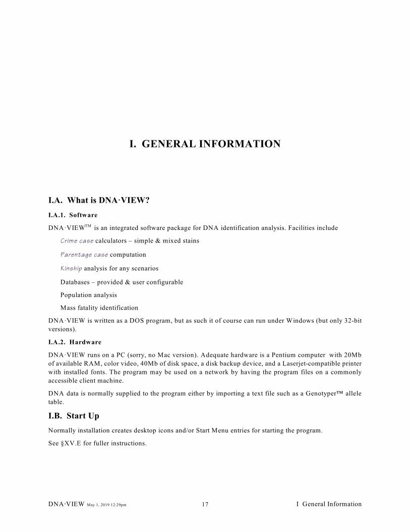
I.A. What is DNA·VIEW?
I.A.1. Software
DNA·VIEW is an integrated software package for DNA identification analysis. Facilities includeTM
Crime case calculators – simple & mixed stains
Parentage case computation
Kinship analysis for any scenarios
Databases – provided & user configurable
Population analysis
Mass fatality identification
DNA·VIEW is written as a DOS program, but as such it of course can run under Windows (but only 32-bit
versions).
I.A.2. Hardware
DNA·VIEW runs on a PC (sorry, no Mac version). Adequate hardware is a Pentium computer with 20Mb
of available RAM, color video, 40Mb of disk space, a disk backup device, and a Laserjet-compatible printer
with installed fonts. The program may be used on a network by having the program files on a commonly
accessible client machine.
DNA data is normally supplied to the program either by importing a text file such as a Genotyper™ allele
table.
I.B. Start Up
Normally installation creates desktop icons and/or Start Menu entries for starting the program.
See §XV.E for fuller instructions.
DNA@VIEW May 1, 2019 12:29pm I General Information17
I.C. Learning DNA·VIEW
I.C.1. Manual and release note
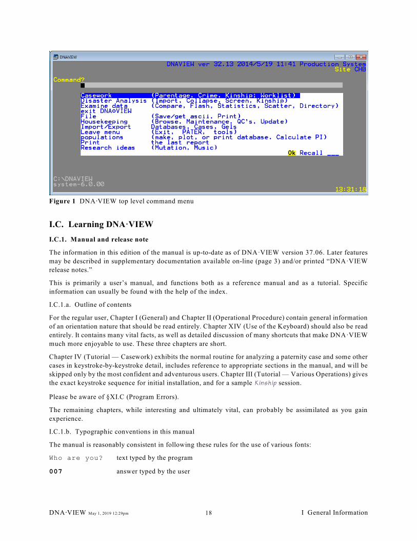
The information in this edition of the manual is up-to-date as of DNA·VIEW version 37.06. Later features
may be described in supplementary documentation available on-line (page 3) and/or printed “DNA·VIEW
release notes.”
This is primarily a user’s manual, and functions both as a reference manual and as a tutorial. Specific
information can usually be found with the help of the index.
I.C.1.a. Outline of contents
For the regular user, Chapter I (General) and Chapter II (Operational Procedure) contain general information
of an orientation nature that should be read entirely. Chapter XIV (Use of the Keyboard) should also be read
entirely. It contains many vital facts, as well as detailed discussion of many shortcuts that make DNA·VIEW
much more enjoyable to use. These three chapters are short.
Chapter IV (Tutorial — Casework) exhibits the normal routine for analyzing a paternity case and some other
cases in keystroke-by-keystroke detail, includes reference to appropriate sections in the manual, and will be
skipped only by the most confident and adventurous users. Chapter III (Tutorial — Various Operations) gives
the exact keystroke sequence for initial installation, and for a sample Kinship session.
Please be aware of §XI.C (Program Errors).
The remaining chapters, while interesting and ultimately vital, can probably be assimilated as you gain
experience.
I.C.1.b. Typographic conventions in this manual
The manual is reasonably consistent in following these rules for the use of various fonts:
Who are you? text typed by the program
007 answer typed by the user
Figure 1 DNA@VIEW top level command menu
DNA@VIEW May 1, 2019 12:29pm I General Information18
DNAVIEW ver 32.13 2014/5/19 11:41 Production SystemWorkstation Foghorn Site CHB
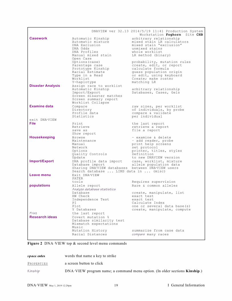
Casework Automatic Kinship arbitrary relationshipAutomatic mixture mixed stain LR calculatorsDNA Exclusion mixed stain “exclusion”DNA Odds unmixed stainsDNA Profiles whole worklistManual mixed stain LR method (binary)Open CaseOptions(case) probability, mutation rulesParentage case create, edit, or reportPrototype Kinship calculate formulaRacial Estimate guess population originType in a Read or edit, using keyboardWorklist Create; make rosterY-haplotype matching LR
Disaster Analysis Assign race to worklistAutomatic Kinship arbitrary relationshipImport/Export Databases, Cases, GelsScreen disaster matchesScreen summary reportWorklist Collapse
Examine data Compare raw sizes, per worklistDirectory of individuals, by probeProfile data compare & validateStatistics per individual
exit DNA@VIEWFile Print the last report
Retrieve retrieve a reportsave as file a reportShow report
Housekeeping Browse – examine & deleteMaintenance – add reader, probeManual print help screensNetwork set protocolOptions printer, titles, stylesQuality Controls DefinitionUpdate to new DNAVIEW version
Import/Export DNA profile data import case, worklist, mixtureDatabase import allele population dataSharing DNA@VIEW databases between DNA@VIEW usersSearch database ... LIMS data in ... (misc)
Leave menu Exit DNA@VIEWPATER tools Requires supervision
populations Allele report Rare & common allelesAnalyze database statisticsDatabase create, manipulate, listHW Check exact testIndependence Test exact testPI Calculate IndexPlot one or several data base(s)Y Databases create, manipulate, compute
Print the last reportResearch ideas Covert mutation %
Database similarity testMismatch expectationsMusicMutation History summarize from case dataRacial Distances compare many races
Figure 2 DNA·VIEW top & second level menu commands
space enter words that name a key to strike
PROPERTIES a screen button to click
Kinship DNA·VIEW program name; a command menu option. (In older sections Kinship.)
DNA@VIEW May 1, 2019 12:29pm I General Information19
Housekeeping A command menu (group of commands).
Edit the locus name lower-level menu option
properties word on a Windows window
I.C.2. Program conventions
I.C.2.a. Menus in DNAAVIEW are always (usually the background) green, and a green background always
is a menu, operated as described in §XIV.A.2, page 287.
I.C.2.b. Enter is usually the right response to any prompt. If a button is highlit (yellow) enter activates it.
I.C.2.c. Esc means back up, or abandon the current operation. Tab and shift-tab cycle the highlight among
the buttons. These are the same as the Windows conventions.
I.C.2.d. A yellow banner on the bottom of the screen indicates that the program is waiting for a keystroke
from the user to continue to the next step.
I.C.2.e. Ctrl-pause means break; abandon the current operation and return to the main menu. Ctrl-c usually
has the same effect (and is a little easier to type).
I.C.3. Telephone and fax assistance
are part of the DNA@VIEW license agreement. The numbers are listed on page 2.
I.C.4. Select program option
Programs are selected from the main (COMMAND) menu shown in 1 and Figure 2. The method of selection
is intuitive, and is explained in detail in §XIV.A.2. §IX.F.3 explains the method of choosing between the
menu styles of the two figures.
DNA@VIEW May 1, 2019 12:29pm I General Information20
I.D. To Exit
I.D.1. From a command
After the selected program finishes, the COMMAND menu will usually reappear.
Some of the programs end leaving information on the screen for you to read. In that case there is a yellow
banner at the bottom right corner. Then you need to Enter (or any key) to release the display.
I.D.2. From graphics mode
DNA@VIEW has some graphics capability mainly for drawing graphs. The graphics mode requires Windows
XP or older (or an appropriate virtual system), and requires starting DNA@VIEW with the special DNA@VIEW
PLOT icon.
The presence of curved lines or pastels on the video screen means that graphics mode is on. Enter should get
you out of graphics mode and into the next program step. If any event ctrl-break will abort immediately to
the COMMAND menu.
I.D.3. From “special editing mode”
A few programs — especially tools — use the built in APL editor (§XIV.B). To abort editing, ctrl-q.
I.D.4. From tools
From the special state called tools, strike F3 to return to the main menu.
I.D.5. To Windows
The menu choice exit DNAAVIEW closes DNA·VIEW.
You don’t need to close DNAAVIEW to use another Windows process. Certain keystrokes that are recognized
by Windows are well worth knowing.
» Alt-tab switches to the next process in sequence. Hold alt and tap the tab key to see the ring of
sequential processes and to select the desired one.
» Alt-enter toggles the DNAAVIEW screen between full-screen and windowed appearance.
I.D.6. (Avoiding) program delays
In various circumstances the program pauses for several seconds to let the user read a message on the screen.
For example, there is a 2-second delay to show the initial banner when DNA·VIEW is started, and a 4-second
delay for any (temporary) errors that are encountered during startup when a new system is first installed.
If you do not feel like being patient, you can hurry the program past these delays by hitting space.
See §XV.E.3.a about avoiding delays in other Windows operations while DNA@VIEW is running.
DNA@VIEW May 1, 2019 12:29pm I General Information21
I.E. The world of DNAAVIEW
I.E.1. Data structures
To understand DNA@VIEW it is helpful to be aware of the various data structures in it.
I.E.1.a. Cases (§V.B, page 41 and §XVI.B.2)
The commands Paternity case, Automatic mixture, and Automatic Kinship (§V.B) group individuals
into cases. Screen disaster matches (§VII.D) expects the references of a family unit to be grouped as
a case.
I.E.1.a.i.) Case numbers
Cases are known by case numbers of digits only. Details in §XIV.A.10.
I.E.1.a.ii.) Roles (Figure 154, page 311)
Each person in a case occupies a role within that case. Roles are single capital letters. Each role letter
has a descriptive word associated with it – “mother” associated with the role “M” for example – but
for most purposes the roles can be used arbitrarily. The person occupying role “M” need not be a
mother.
Only one person may occupy any one role in a case. The role-letter + case-number thus represents
an alternative way – besides the sample number – to refer to a sample.
A person may belong to more than one case and/or simultaneously occupy different roles in a single
case.
I.E.1.a.iii.) Language
The set of available roles, and the associated descriptive words, depend on the language or genre of
a case. The possible genres are paternity, maternity, kinship, and crime (Figure 154).
I.E.1.a.iv.) Miscellaneous other data associated with a case include:
» case comment (arbitrary and searchable)
» comment per role – typically the name of a person or description of a unknown sample
» computation race(s)
I.E.1.a.v.) NOT part of a case: DNA profiles. The case links to DNA profiles through the individuals
(§I.E.1.b.iii) in the case, but the profile data is not stored as part of the case.
I.E.1.b. Individuals/samples (§XIV.A.9, §XVI.B.1)
People or samples can be found as a role in some case, or can exist independently of any case as an
orphan. For that matter, the same person can be in several different cases or even occupy more than one
role in one case.
I.E.1.b.i.) Two ways to identify a sample
» If a sample occupies a role in a case, then it can also be designated by using the case number + the
role letter (§I.E.1.b.ii).
» Its sample (or accession) number (§I.E.1.b.iii) can be used to identify any sample, including
orphans.
I.E.1.b.ii.) Case + role (§X.A.8.b and §XIV.A.9.a.iii)
The notation 61234 M refers to role M of case number 61234. The number is clearly a case number
and not a sample number because it doesn’t have a dash in it. This method of identifying an
DNA@VIEW May 1, 2019 12:29pm I General Information22
individual is convenient for preparation of data input files (§X.A.8.c), for user-selection on-screen
of a profile for calculation (§XIV.A.9.a.iii), and is preferred by the DNA@VIEW programs for display.
I.E.1.b.iii.) Sample/accession number (§XIV.A.9.a)
The accession number is number with a dash ( - ) in it that is formatted like 2009!01234. There may
be up to 4 digits before the dash (a year for example) and up to five digits after. (For data entry
purposes leading 0's in either part are not significant.)
Some laboratories like to assign accession numbers that reflect the case number. Hence the mother,
child, and alleged father in paternity case 444 might be 2000!04441, 2000!04442, and 2000!04449.
Other laboratories assign consecutive numbers without regard to case. The people accessioned in
2000 might be 2000!00001 through 2000!02468. Recommendation: If sequential numbers are
used, I advise continuing with 2001!02469 in the next year, etc., so that the sequence part of the
number won’t repeat for several years. This helps to avoid mistakes.
I.E.1.c. Worklist
A worklist or roster (formerly called membrane) consists of a number of lanes, which typically
correspond to the lanes or capillaries of an electrophoresis run in the laboratory. A worklist may have
only a few lanes (minimum of one), or may be defined with thousands of lanes.
Each lane may be labeled with a sample (or accession or person) number, as described in §I.E.1.b.iii, or
with an allelic ladder (in case of GeneScan™ data), or may be unlabeled.
The roster is thus an arbitrary list of people. Each person may incidentally be defined as part of some case
(paternity, crime, or kinship), or of several different cases, or of no case at all.
The people in a case do not need to be grouped together on the same worklist. A person may even be
assayed on several different lanes or worklists, in which case the user has flexibility in analysis whether
to use a particular assay (§V.B.26) or to check for a consensus among all assays.
I.E.1.c.i.) Worklist maintenance
The Worklist command (§V.J, page 92) can create or delete or edit a worklist, including editing the
roster of sample numbers.
Import/Export options such as Genotyper import (§X.A.1 page 226) or Hitachi STRCall import
(§X.A.6, page 232) also can create a worklist and populate the roster.
I.E.1.d. Read (DNA genotypes for 1 locus, multiple samples)
Each lane of a worklist potentially has a DNA profile associated with it. The DNA data is stored as reads.
Each read is the data for one locus and all the lanes of a worklist. Thus if for example the CODIS loci are
used a worklist might have 13 or 14 loci associated with it. There is no limit, though, and it is also
permitted to have multiple reads for the same locus.
The data for each read is, like the worklist, organized into lanes or capillaries. Each lane may have zero
or more bands or alleles. Bands associated with unlabeled lanes are not accessible by or used by any
analysis program, but a lane label can always be added.
Each read has a 3-digit reader number associated with it, which identifies the technician responsible for
creating it.
I.E.1.d.i.) Read maintenance
The command Type in a Read (§IV.D.4) permits manual creation or editing of reads. But usually, if
you do need to enter data manually, it’s easier to use Bill Gates’ fine Excel program and ...
DNA@VIEW May 1, 2019 12:29pm I General Information23
Import/Export options such as Genotyper import(§X.A.1 page 226) or Hitachi STRCall import
(§X.A.6, page 232) import allele sizes and save them as reads.
I.E.1.e. Loci (§IX.B, page 201)
DNAAVIEW has an extensible list of loci. (Usually users don’t need to add new loci though, as all the
known ones are already included or are automatically added along with software updates.)
Associated with each locus is a variety of parameters such as repeat amount (e.g. 4 for tetramers), spelling
of the name (e.g. vWA or VWA) and notation rules (e.g. STR alleles are usually numbered; SNP alleles
are nucleotide letters).
I.E.1.e.i.) Locus maintenance is via the Probe/locus parameters option of the Maintenance command
in the menu, or by using the * key to select a locus from the locus menu in any context.
I.E.1.f. Races (§XIV.A.9.a.iii, page 293)
DNAAVIEW accommodates 52 races, corresponding to the letters a-z, A-Z, plus one “unknown/child”
category denoted by a dash (!). The user may associate any race name desired with each letter.
I.E.1.f.i.) Maintenance of the race list is via the codings for races option of the Maintenance command
in the Housekeeping menu, or by striking ? whenever a race letter is to be provided in response
to a prompt.
I.E.1.g. Allele probability databases
A large number of reference allele population databases are delivered with DNAAVIEW, and more may
be added in various ways. There may be several databases even for a particular locus and racial/ethnic
group, but only one among them may carry at any given time a special tag denoting that it is the “default”
database to be used for probability computations for that race/locus combination.
I.E.1.g.i.) Database maintenance
The Database command (§VIII.C, page 158, in the Populations menu) has options (among others)
to
» compile a database from DNAAVIEW data (i.e. compile it from Reads)
» Edit or Type in data to create a database
» rename, delete, or set default status of a database
» perform various statistical analyses
The Import/Export command has options to import a database in various formats.
Plot creates graphs and histograms of allele frequencies.
I.E.2. Casework Analysis
DNAAVIEW has several commands to analyze cases of different kinds and in different ways. Each of them
operates on a selected case (§I.E.1.a) that has a collection of roles with sample numbers attached. Assuming
that the sample numbers also appear in some worklist roster (§I.E.1.c), the DNA profiles for the various
individuals in the case are brought together for the analysis
I.E.2.a. Paternity/maternity case
The typical paternity trio case, or common variations of it such as missing mother or maternity, are most
easily and thoroughly analyzed by the Paternity case command (§V.B, page41). It operates on a has
DNA@VIEW May 1, 2019 12:29pm I General Information24
roles designating mother (usually), child or children, and alleged man or men. Per trio it performs the
analysis locus by locus and prepares an informal and a formal report of the results.
I.E.2.a.i.) PATER interface
Additionally, the results of the analysis are written to an external table (documentation available)
which can be conveniently interpreted by another program. The PATER program is one option for
creating a suitable lay-person/court friendly report.
I.E.2.b. Kinship
The paternity trio is one example of an infinitude of kinship problem – deciding how strongly the DNA
evidence favors one or another arbitrary alternate hypotheses as to how a collection of people might be
related.
The general problem is analyzed by the immigration/kinship (§VI.E, page 109) sub-option of Automatic
kinship (or for that matter of Parentage case or Automatic mixture).
I.E.2.c. Mixed stain (revised – 2014)
Automatic mixture includes several tools for mixture analysis:
I.E.2.c.i.) Mixture calculator (§V.D, page 65) computes a likelihood ratio for a mixed stain under the
“binary model” (each allele is present or not).
I.E.2.c.ii.) Mixture Solution (under development) is a full-fledged “continuous model” (dropout,
intensity, stutter, drop-in aware) mixture calculator.
I.E.2.c.iii.) Mixture explorer (experimental) very quickly guesses which references are associated with
a mixture.
I.E.3. Disaster Screening
Screen disaster matches (§VII.D) and other programs including Automatic Kinship are useful for mass
fatality investigations.
I.E.4. Single-profile or manual crime stain analysis
There are also several options for crime stain analysis that operate either on a single individual named by
sample number, or on a DNA profile typed immediately in.
I.E.4.a. profile probability – calculate a simple stain
The DNA Odds command (§V.G, page 84) computes profile odds for a single profile at a time, and allows
a variety of computation options such as those recommended in the NRC II report, for autosomal loci.
Y-haplotype matching LR (§V.H, page 87) performs a similar computation for Y-haplotypes.
I.E.4.b. mixtures
DNA exclusion (§V.I, page 89) computes the “probability of exclusion” for a specified mixture of alleles
at a collection of autosomal loci.
The stand-alone Manual mixed stain , like the symbolic mixture calculator option of Automatic mixture,
computes a likelihood ratio for a mixture. However, it works strictly on typed-in data.
DNA@VIEW May 1, 2019 12:29pm I General Information25
I.E.5. Prototype Kinship
Kinship (§VI.J, page 134) is a stand-alone command that is the original, prototype version of the automatic
version (§I.E.2.b).
I.E.6. Database analysis
Several commands do population or population-genetic analyses.
I.E.6.a. Racial Distance
I.E.6.b. HW Check and Independence test
These commands test population studies for evidence of non-independence. The input is in from a text
file.
I.E.6.c. Database statistics
The command (also Database option) Analyze database statistics and the command Allele report
compute various statistics and summaries based on DNAAVIEW databases.
Y-haplotype database statistics (§VIII.F.5) computes useful statistics for the Y databases.
I.E.7. Reports in DNAAVIEW
Many DNAAVIEW operations produce a report. The report resides in the “report buffer” until it is supplanted
by another report. In the meantime, the report can be (§V.K) printed (Print), viewed (Show report), or saved
as a file (Save as).
DNA@VIEW May 1, 2019 12:29pm I General Information26
I.E.8. Where to Find It — Sub-menus
Many commands do a specific thing. Others do a number of related operations, as indicated in these sub-
menus:
Browse – (examine & delete) Reads, Lanes, Stan-
dards Ladders, Configurations
Options – control printing, report formats, national
Keyboard & Language. Set Case Options.
Paternity/Automatic Kinship/Automatic mixture –
retrieve, modify, analyze cases. Set Case Op-
tions. Kinship and simulations.
Maintenance – lists etc. Examine & modify loci,
races, network preferences. Paradox info, main-
tenance. Record/compare "switch" settings.
Database – allele population samples. Compile,
recompile, Analyze database statistics, Delete
or rename, Edit a database, Set default data-
base, per race, Type in data to create a data-
base
Plot – data base(s); DISPLAY (screen), METAFIL
(file) printer, more plots, fewer plots, probability
of paternity
Quality Control – add control, disenroll control,
e d i t
stats, range report, recompute
Import/export < DNA profile data import
ABI import: GeneMapper, Genotyper
Hitachi STRCall import
Import/export < Database import from table
import publication format: Allele frequency
( o r
count) population database import
import reference genotypes and build tables
Import/export < Sharing DNA@VIEW databases
transfer between users: DNA@VIEW Frequency
Database import and export
Import/export < miscellaneous
List and search database profiles
Case and Accession data import
DNA@VIEW May 1, 2019 12:29pm I General Information27
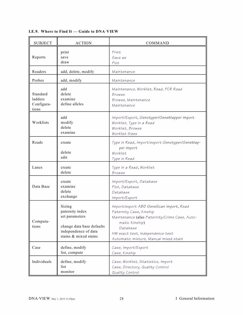
I.E.9. Where to Find It — Guide to DNA·VIEW
SUBJECT ACTION COMMAND
Reports
save
draw
Save as
Plot
Readers add, delete, modify Maintenance
Probes add, modify Maintenance
Standard
ladders
Configura-
tions
add
delete
examine
define alleles
Maintenance, Worklist, Read, PCR Read
Browse
Browse, Maintenance
Maintenance
Worklists
add
modify
delete
examine
Import/Export , Genotyper/GeneMapper import
Worklist, Type in a Read
Worklist, Browse
Worklist Sizes
Reads create
delete
edit
Type in Read , Import/export Genotyper/GeneMap-
per import
Worklist
Type in Read
Lanes create
delete
Type in a Read , Worklist
Browse
Data Base
create
examine
delete
exchange
Import/Export , Database
Plot, Database
Database
Import/Export
Computa-
tions
Sizing
paternity index
set parameters
change data base defaults
independence of data
stains & mixed stains
Import/export ABD GeneScan import, Read
Paternity Case, Kinship
Maintenance (also Paternity/Crime Case, Auto-
matic Kinship)
Database
HW exact test, Independence test
Automatic mixture, Manual mixed stain
Case define, modify
list, compute
Case, Import/Export
Case, Kinship
Individuals define, modify
list
monitor
Case, Worklist, Statistics, Import
Case, Directory, Quality Control
Quality Control
DNA@VIEW May 1, 2019 12:29pm I General Information28
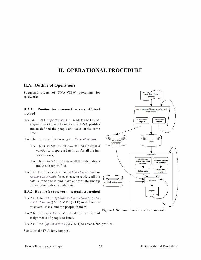
Figure 3 Schematic workflow for casework
II. OPERATIONAL PROCEDURE
II.A. Outline of Operations
Suggested orders of DNA·VIEW operations for
casework:
II.A.1. Routine for casework – very efficient
method
II.A.1.a. Use Import/export < Genotyper (Gene-
Mapper, etc) import to import the DNA profiles
and to defined the people and cases at the same
time.
II.A.1.b. For paternity cases, go to Paternity case
II.A.1.b.i.) batch select, add the cases from a
worklist to prepare a batch run for all the im-
ported cases,
II.A.1.b.ii.) batch run to make all the calculations
and create report files.
II.A.1.c. For other cases, use Automatic mixture or
Automatic kinship for each case to retrieve all the
data, summarize it, and make appropriate kinship
or matching index calculations.
II.A.2. Routine for casework – second best method
II.A.2.a. Use Paternity/Automatic mixture or Auto-
matic Kinship (§V.B/§V.D, §VI.F) to define one
or several cases, and the people in them.
II.A.2.b. Use Worklist (§V.J) to define a roster of
assignments of people to lanes.
II.A.2.c. Use Type in a Read (§IV.D.4) to enter DNA profiles.
See tutorial §IV.A for examples.
DNA@VIEW May 1, 2019 12:29pm II Operational Procedure29
II.A.3. Occasional operations
II.A.3.a. Maintaining allele frequencies includes some of the following tasks:
II.A.3.a.i.) Compiling the accumulated casework (or other) data into sets of allele population frequencies
is done using Database (§VIII.C). Compare (§IX.H), Statistics (§IX.D ), and Browse (§IX.E) are
used to analyze problems and clean up the data, as explained in §VIII.C.8.a, “Analyzing exception
reports.”
II.A.3.a.ii.) Import/Export (automatic) and Database (manual) are used to install databases from other
sources.
II.A.3.a.iii.) Various analysis and statistical capabilities are in Database, HW Check, and Allele report.
II.A.3.a.iv.) Plot (§VIII.E) is a very useful tool for gaining knowledge and insight.
DNA@VIEW May 1, 2019 12:29pm II Operational Procedure30
II.B. Preliminaries — details
More details of the steps discussed below are given in the Tutorial (Chapter IV). These setup operations have
been pre-configured as part of system customization insofar as possible, and the remaining ones can more
or less be postponed.
II.B.1. List of loci
The locus list is probably adequately preconfigured as part of system customization. It can also be configured
“on-the-fly” – i.e., as needed. §IX.B explains loci in DNAAVIEW. The critical issues are
II.B.1.a. Locus list arranged as desired. The loci are most conveniently and easily activated and arranged in
order with the REORDER: MPLX button (§IX.B.1.d.i). See also §IX.B.1.e.
II.B.1.b. Set parameters
Key parameters for PCR systems include: repeat amount, notation style (i.e. numbered alleles, SNP
notation, Amelogenin, Polymarkers), mutation rate.
The parameters can also be defined or modified any time the locus menu appears (via PROPERTIES).
II.B.2. List of races
The race list can be accessed via the EDIT RACES button in response to a race-letter request by the program,
so pre-configuration is unnecessary. You can also use Maintenance, codings for races to make sure that race
names exist for each race letter that you will use.
II.B.3. Default data base
Whenever allele probabilities are needed as part of some computation in DNAAVIEW, the program checks
to see if a “default” has been established for the locus and race at issue. The facilities for default databases
are explained in §VIII.C.2.
II.B.4. List of readers
“Readers” are technicians who use the program. Readers can be added as needed on the fly (§IX.A.5.b), or
a list of them can be built as a separate operation using the Maintenance command in Housekeeping,
option readers – §IX.A.5.
II.B.5. Define Quality Controls
To take advantage of quality control monitoring, use Quality Control (§IX.J) to enroll accession numbers
for quality control samples.
II.B.6. Miscellaneous options
Several of the Options §IX.F (Housekeeping menu), may be useful.
II.B.6.a.i.) They include formatting of dates, case numbers, numbers (i.e. 1.35 vs. 1,35) and alleles;
keyboard configuration, language for prompts, printer options.
II.B.6.a.ii. Especially check the Case options, §V.C. Select Options, Options from “Case”, and make sure
that all the values are acceptable.
DNA@VIEW May 1, 2019 12:29pm II Operational Procedure31

DNA@VIEW May 1, 2019 12:29pm II Operational Procedure32
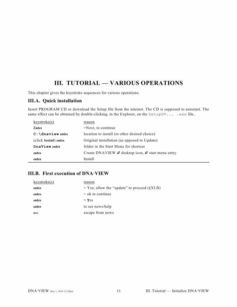
III. TUTORIAL — VARIOUS OPERATIONS
This chapter gives the keystroke sequences for various operations.
III.A. Quick installation
Insert PROGRAM CD or download the Setup file from the internet. The CD is supposed to autostart. The
same effect can be obtained by double-clicking, in the Explorer, on the SetupDV... .exe file..
keystroke(s) reason
Enter =Next, to continue
C:\dnaview enter location to install (or other desired choice)
(click Install) enter Original installation (as opposed to Update)
DnaView enter folder in the Start Menu for shortcut
enter Create DNAVIEW T9 desktop icon, T9 start menu entry
enter Install
III.B. First execution of DNA·VIEW
keystroke(s) reason
enter = Yes; allow the “update” to proceed (§XI.B)
enter = ok to continue
enter = Yes
enter to see news/help
esc escape from news
DNA@VIEW May 1, 2019 12:29pm III. Tutorial — Initialize DNA@VIEW33
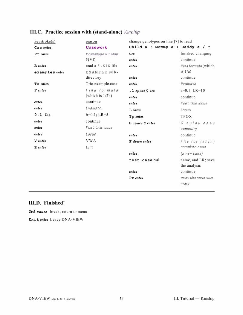
III.C. Practice session with (stand-alone) Kinship
keystroke(s) reason
Cas enter Casework
Pr enter Prototype Kinship
(§VI)
R enter read a *.KIN file
examples enter E X A M P L E s u b -
directory
Tr enter Trio example case
F enter F i n d f o r m u l a
(which is 1/2b)
enter continue
enter Evaluate
0.1 Esc b=0.1; LR=5
enter continue
enter Post this locus
enter Locus
V enter VWA
E enter Edit
change genotypes on line [7] to read
Child a : Mommy a + Daddy a / ?
Esc finished changing
enter continue
enter Find formula (which
is 1/a)
enter continue
enter Evaluate
.1 space 0 esc a=0.1; LR=10
enter continue
enter Post this locus
L enter Locus
Tp enter TPOX
D space c enter D i s p l a y c a s e
summary
enter continue
F down enter F i l e ( o r f e t c h )
complete case
enter (a new case)
test case tab name, and LR; save
the analysis
enter continue
Pr enter print the case sum-
mary
III.D. Finished!
Ctrl-pause break; return to menu
Exit enter Leave DNA·VIEW
DNA@VIEW May 1, 2019 12:29pm III. Tutorial — Kinship34
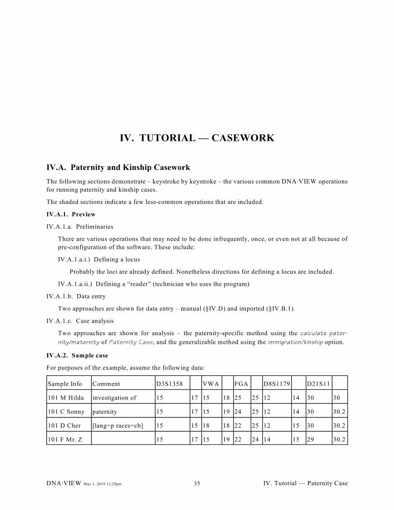
IV. TUTORIAL — CASEWORK
IV.A. Paternity and Kinship Casework
The following sections demonstrate – keystroke by keystroke – the various common DNAAVIEW operations
for running paternity and kinship cases.
The shaded sections indicate a few less-common operations that are included.
IV.A.1. Preview
IV.A.1.a. Preliminaries
There are various operations that may need to be done infrequently, once, or even not at all because of
pre-configuration of the software. These include:
IV.A.1.a.i.) Defining a locus
Probably the loci are already defined. Nonetheless directions for defining a locus are included.
IV.A.1.a.ii.) Defining a “reader” (technician who uses the program)
IV.A.1.b. Data entry
Two approaches are shown for data entry – manual (§IV.D) and imported (§IV.B.1).
IV.A.1.c. Case analysis
Two approaches are shown for analysis – the paternity-specific method using the calculate pater-
nity/maternity of Paternity Case, and the generalizable method using the immigration/kinship option.
IV.A.2. Sample case
For purposes of the example, assume the following data:
Sample Info Comment D3S1358 VWA FGA D8S1179 D21S11
101 M Hilda investigation of 15 17 15 18 25 25 12 14 30 30
101 C Sonny paternity 15 17 15 19 24 25 12 14 30 30.2
101 D Cher [lang=p races=cb] 15 15 18 18 22 25 12 15 30 30.2
101 F Mr. Z 15 17 15 19 22 24 14 15 29 30.2
DNA@VIEW May 1, 2019 12:29pm IV. Tutorial — Paternity Case35
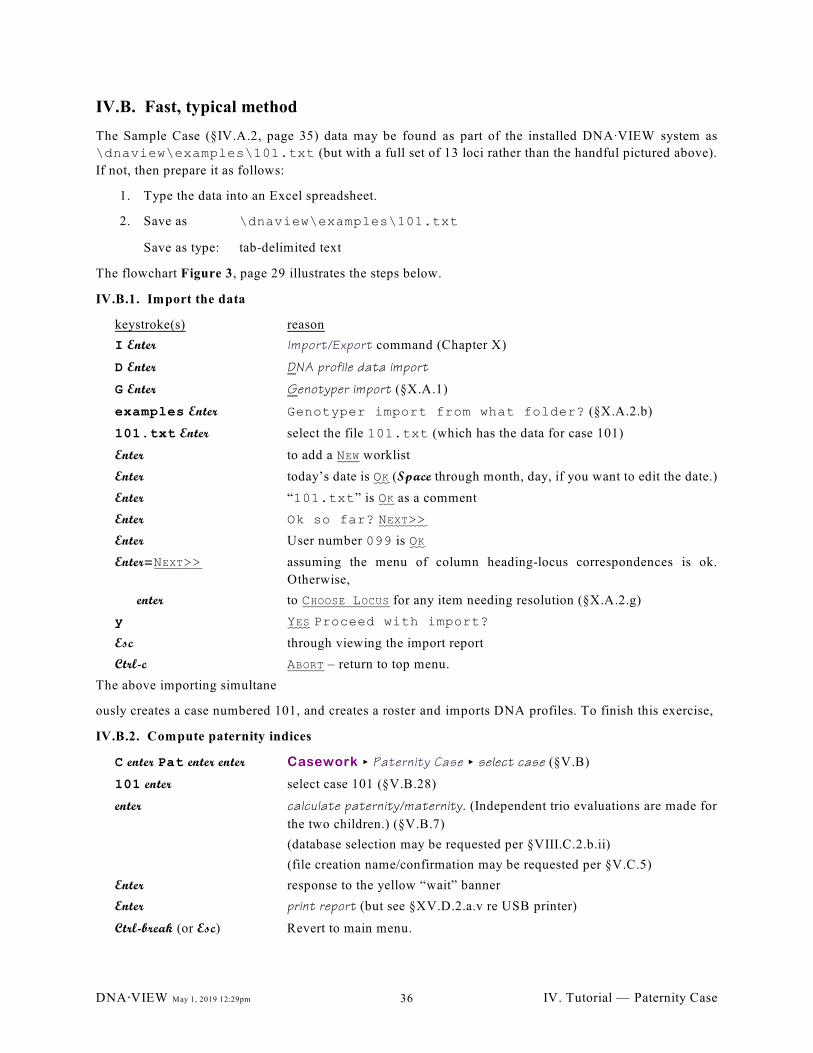
IV.B. Fast, typical method
The Sample Case (§IV.A.2, page 35) data may be found as part of the installed DNAAVIEW system as
\dnaview\examples\101.txt (but with a full set of 13 loci rather than the handful pictured above).
If not, then prepare it as follows:
1. Type the data into an Excel spreadsheet.
2. Save as \dnaview\examples\101.txt
Save as type: tab-delimited text
The flowchart Figure 3, page 29 illustrates the steps below.
IV.B.1. Import the data
keystroke(s) reason
I Enter Import/Export command (Chapter X)
D Enter DNA profile data import
G Enter Genotyper import (§X.A.1)
examples Enter Genotyper import from what folder? (§X.A.2.b)
101.txt Enter select the file 101.txt (which has the data for case 101)
Enter to add a NEW worklist
Enter today’s date is OK (Space through month, day, if you want to edit the date.)
Enter “101.txt” is OK as a comment
Enter Ok so far? NEXT>>
Enter User number 099 is OK
Enter=NEXT>> assuming the menu of column heading-locus correspondences is ok.
Otherwise,
enter to CHOOSE LOCUS for any item needing resolution (§X.A.2.g)
y YES Proceed with import?
Esc through viewing the import report
Ctrl-c ABORT – return to top menu.
The above importing simultane
ously creates a case numbered 101, and creates a roster and imports DNA profiles. To finish this exercise,
IV.B.2. Compute paternity indices
C enter Pat enter enter Casework < Paternity Case < select case (§V.B)
101 enter select case 101 (§V.B.28)
enter calculate paternity/maternity. (Independent trio evaluations are made for
the two children.) (§V.B.7)
(database selection may be requested per §VIII.C.2.b.ii)
(file creation name/confirmation may be requested per §V.C.5)
Enter response to the yellow “wait” banner
Enter print report (but see §XV.D.2.a.v re USB printer)
Ctrl-break (or Esc) Revert to main menu.
DNA@VIEW May 1, 2019 12:29pm IV. Tutorial — Paternity Case36
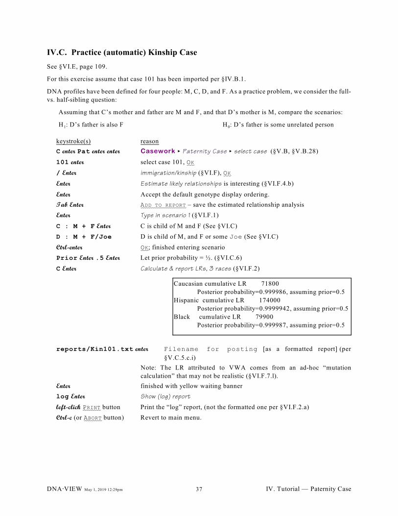
Caucasian cumulative LR 71800
Posterior probability=0.999986, assuming prior=0.5
Hispanic cumulative LR 174000
Posterior probability=0.9999942, assuming prior=0.5
Black cumulative LR 79900
Posterior probability=0.999987, assuming prior=0.5
IV.C. Practice (automatic) Kinship Case
See §VI.E, page 109.
For this exercise assume that case 101 has been imported per §IV.B.1.
DNA profiles have been defined for four people: M, C, D, and F. As a practice problem, we consider the full-
vs. half-sibling question:
Assuming that C’s mother and father are M and F, and that D’s mother is M, compare the scenarios:
1 0H : D’s father is also F H : D’s father is some unrelated person
keystroke(s) reason
C enter Pat enter enter Casework < Paternity Case < select case (§V.B, §V.B.28)
101 enter select case 101, OK
/ Enter immigration/kinship (§VI.F), OK
Enter Estimate likely relationships is interesting (§VI.F.4.b)
Enter Accept the default genotype display ordering.
Tab Enter ADD TO REPORT – save the estimated relationship analysis
Enter Type in scenario 1 (§VI.F.1)
C : M + F Enter C is child of M and F (See §VI.C)
D : M + F/Joe D is child of M, and F or some Joe (See §VI.C)
Ctrl-enter OK; finished entering scenario
Prior Enter .5 Enter Let prior probability = ½. (§VI.C.6)
C Enter Calculate & report LRs, 3 races (§VI.F.2)
reports/Kin101.txt enter Filename for posting [as a formatted report] (per
§V.C.5.c.i)
Note: The LR attributed to VWA comes from an ad-hoc “mutation
calculation” that may not be realistic (§VI.F.7.l).
Enter finished with yellow waiting banner
log Enter Show (log) report
left-click PRINT button Print the “log” report, (not the formatted one per §VI.F.2.a)
Ctrl-c (or ABORT button) Revert to main menu.
DNA@VIEW May 1, 2019 12:29pm IV. Tutorial — Paternity Case37
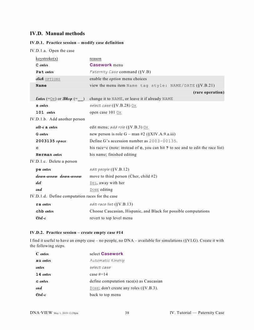
IV.D. Manual methods
IV.D.1. Practice session – modify case definition
IV.D.1.a. Open the case
keystroke(s) reason
C enter Casework menu
Pat enter Paternity Case command (§V.B)
click OPTIONS enable the option menu choices
Name view the menu item Name tag style: NAME/DATE (§V.B.21)
(rare operation)
Enter (=OK) or Bksp (=__) change it to NAME, or leave it if already NAME
s enter select case (§V.B.28) OK
101 enter open case 101 OK
IV.D.1.b. Add another person
alt-e a enter edit menu; add role (§V.B.3) OK
G enter new person is role G – man #2 (§XIV.A.9.a.iii)
2003135 space Define G’s accession number as 2003-00135.
c his race=c (note: instead of c, you can hit ? to see and to edit the race list)
Herman enter his name; finished editing
IV.D.1.c. Delete a person
pe enter edit people (§V.B.12)
down-arrow down-arrow move to third person (Cher, child #2)
del DEL, away with her
end DONE editing
IV.D.1.d. Define computation races for the case
ra enter edit race list (§V.B.13)
chb enter Choose Caucasian, Hispanic, and Black for possible computations
Ctrl-c revert to top level menu
IV.D.2. Practice session – create empty case #14
I find it useful to have an empty case – no people, no DNA – available for simulations (§VI.G). Create it with
the following steps.
C enter select Casework
au enter Automatic Kinship
enter select case
14 enter case #=14
c enter define computation race(s) as Caucasian
end DONE; don't create any roles (§V.B.3).
Ctrl-c back to top menu
DNA@VIEW May 1, 2019 12:29pm IV. Tutorial — Paternity Case38
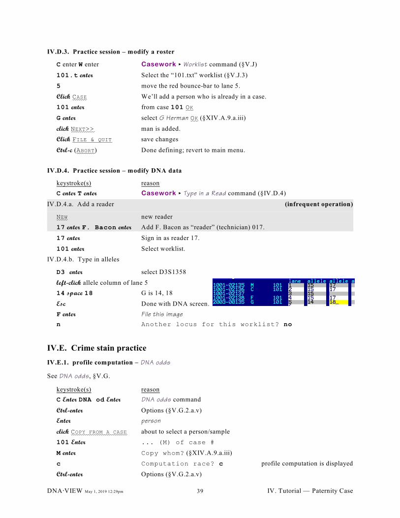
IV.D.3. Practice session – modify a roster
C enter W enter Casework < Worklist command (§V.J)
101.t enter Select the “101.txt” worklist (§V.J.3)
5 move the red bounce-bar to lane 5.
Click CASE We’ll add a person who is already in a case.
101 enter from case 101 OK
G enter select G Herman OK (§XIV.A.9.a.iii)
click NEXT>> man is added.
Click FILE & QUIT save changes
Ctrl-c (ABORT) Done defining; revert to main menu.
IV.D.4. Practice session – modify DNA data
keystroke(s) reason
C enter T enter Casework < Type in a Read command (§IV.D.4)
IV.D.4.a. Add a reader (infrequent operation)
NEW new reader
17 enter F. Bacon enter Add F. Bacon as “reader” (technician) 017.
17 enter Sign in as reader 17.
101 enter Select worklist.
IV.D.4.b. Type in alleles
D3 enter select D3S1358
left-click allele column of lane 5
14 space 18 G is 14, 18
Esc Done with DNA screen.
F enter File this image
n Another locus for this worklist? no
IV.E. Crime stain practice
IV.E.1. profile computation – DNA odds
See DNA odds, §V.G.
keystroke(s) reason
C Enter DNA od Enter DNA odds command
Ctrl-enter Options (§V.G.2.a.v)
Enter person
click COPY FROM A CASE about to select a person/sample
101 Enter ... (M) of case #
M enter Copy whom? (§XIV.A.9.a.iii)
c Computation race? c profile computation is displayed
Ctrl-enter Options (§V.G.2.a.v)
DNA@VIEW May 1, 2019 12:29pm IV. Tutorial — Paternity Case39
click PRINT REPRT Print report
To modify the computation, use the mouse (single click to navigate) to select fields such as race, modality,
theta, etc.
Ctrl-c Revert to top menu
IV.F. Some maintenance operations
IV.F.1.a. Establish locus multiplex (rare operation)
H enter Select the Housekeeping menu
M enter Maintenance command (§IX.A)
l enter locus parameters & preferences (§IX.B)
REORDER: MPLX Look at menu of multiplexes. (§IX.B.1.d.i)
Ident enter Ensure Identifiler loci are active and PUT THESE AT TOP of the menu
D3S Highlight the locus D3S1358
IV.F.1.b. Define parameters for a locus (rare operation)
PROPERTIES properties screen for the locus D3S1358
IV.F.1.b.i.) Define the pseudo-enzyme for the locus as “STR”(probably redundant)
Ass enter Assign enzyme (or PCR status) to this locus
STR enter Define the locus as an STR
IV.F.1.b.ii.) Establish the repeat amount and the (often irrelevant) amplicon size
P enter PCR parameters
66 enter 4 enter 66=size of “allele #0”, 4=tetrameric STR
0 enter 0 enter 0 enter 0 enter choose notation style=STR, plus some often irrelevant parameters
1 enter Genetic type is “autosomal”
IV.F.1.b.iii.) Discrete allele system (i.e. measurement uncertainty=0)
W enter 0enter0enter0enter0enter0enter Window size parameters (measurement uncertainty etc.)
C enter Copy window-type params to similar loci (i.e. other STR’s)
Esc esc esc finish with locus properties, with exercise
DNA@VIEW May 1, 2019 12:29pm IV. Tutorial — Paternity Case40
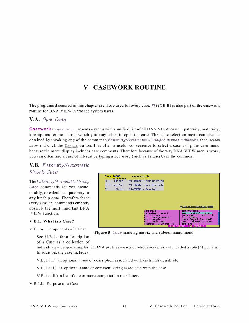
Figure 5 Case nametag matrix and subcommand menu
V. CASEWORK ROUTINE
The programs discussed in this chapter are those used for every case. PI (§XII.B) is also part of the casework
routine for DNA·VIEW Abridged system users.
V.A. Open Case
Casework < Open Case presents a menu with a unified list of all DNA@VIEW cases – paternity, maternity,
kinship, and crime – from which you may select to open the case. The same selection menu can also be
obtained by invoking any of the commands Paternity/Automatic Kinship/Automatic mixture, then select
case and click the SEARCH button. It is often a useful convenience to select a case using the case menu
because the menu display includes case comments. Therefore because of the way DNA@VIEW menus work,
you can often find a case of interest by typing a key word (such as incest) in the comment.
V.B. Paternity/Automatic
Kinship Case
The Paternity/Automatic Kinship
Case commands let you create,
modify, or calculate a paternity or
any kinship case. Therefore these
(very similar) commands embody
possibly the most important DNA
AVIEW function.
V.B.1. What is a Case?
V.B.1.a. Components of a Case
See §I.E.1.a for a description
of a Case as a collection of
individuals – people, samples, or DNA profiles – each of whom occupies a slot called a role (§I.E.1.a.ii).
In addition, the case includes:
V.B.1.a.i.) an optional name or description associated with each individual/role
V.B.1.a.ii.) an optional name or comment string associated with the case
V.B.1.a.iii.) a list of one or more computation race letters.
V.B.1.b. Purpose of a Case
DNA@VIEW May 1, 2019 12:29pm V. Casework Routine — Paternity Case41
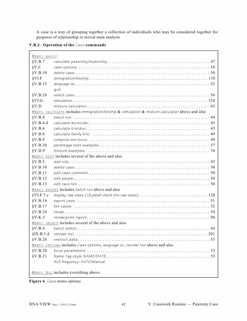
MENU: BASIC:
§V.B.7 calculate paternity/maternity. . . . . . . . . . . . . . . . . . . . . . . . . . . . . . . . . . . . . . . . . . . . . . 47
§V.C case options. . . . . . . . . . . . . . . . . . . . . . . . . . . . . . . . . . . . . . . . . . . . . . . . . . . . . . . . . . . . 58
§V.B.10 delete case. . . . . . . . . . . . . . . . . . . . . . . . . . . . . . . . . . . . . . . . . . . . . . . . . . . . . . . . . . . . . 50
§VI.F immigration/kinship. . . . . . . . . . . . . . . . . . . . . . . . . . . . . . . . . . . . . . . . . . . . . . . . . . . . . . 110
§V.B.15 language is:. . . . . . . . . . . . . . . . . . . . . . . . . . . . . . . . . . . . . . . . . . . . . . . . . . . . . . . . . . . . . 52
quit
§V.B.28 select case. . . . . . . . . . . . . . . . . . . . . . . . . . . . . . . . . . . . . . . . . . . . . . . . . . . . . . . . . . . . . 56
§VI.G simulation. . . . . . . . . . . . . . . . . . . . . . . . . . . . . . . . . . . . . . . . . . . . . . . . . . . . . . . . . . . . . 124
§V.D mixture calculator. . . . . . . . . . . . . . . . . . . . . . . . . . . . . . . . . . . . . . . . . . . . . . . . . . . . . . . . 65
MENU: CALCULATE includes immigration/kinship & simulation & mixture calculator above and also
§V.B.4 batch run. . . . . . . . . . . . . . . . . . . . . . . . . . . . . . . . . . . . . . . . . . . . . . . . . . . . . . . . . . . . . . 44
§V.B.4.d calculate avuncular. . . . . . . . . . . . . . . . . . . . . . . . . . . . . . . . . . . . . . . . . . . . . . . . . . . . . . . 45
§V.B.6 calculate trio/duo. . . . . . . . . . . . . . . . . . . . . . . . . . . . . . . . . . . . . . . . . . . . . . . . . . . . . . . . 45
§V.B.8 calculate family trio. . . . . . . . . . . . . . . . . . . . . . . . . . . . . . . . . . . . . . . . . . . . . . . . . . . . . . 49
§V.B.9 compute one locus. . . . . . . . . . . . . . . . . . . . . . . . . . . . . . . . . . . . . . . . . . . . . . . . . . . . . . . 49
§V.B.30 parentage test examples. . . . . . . . . . . . . . . . . . . . . . . . . . . . . . . . . . . . . . . . . . . . . . . . . . 57
§V.D.9 mixture examples. . . . . . . . . . . . . . . . . . . . . . . . . . . . . . . . . . . . . . . . . . . . . . . . . . . . . . . . 76
MENU: EDIT includes several of the above and also
§V.B.3 add role. . . . . . . . . . . . . . . . . . . . . . . . . . . . . . . . . . . . . . . . . . . . . . . . . . . . . . . . . . . . . . . . 43
§V.B.10 delete case. . . . . . . . . . . . . . . . . . . . . . . . . . . . . . . . . . . . . . . . . . . . . . . . . . . . . . . . . . . . . 50
§V.B.11 edit case comment. . . . . . . . . . . . . . . . . . . . . . . . . . . . . . . . . . . . . . . . . . . . . . . . . . . . . . . 50
§V.B.12 edit people. . . . . . . . . . . . . . . . . . . . . . . . . . . . . . . . . . . . . . . . . . . . . . . . . . . . . . . . . . . . . . 50
§V.B.13 edit race list. . . . . . . . . . . . . . . . . . . . . . . . . . . . . . . . . . . . . . . . . . . . . . . . . . . . . . . . . . . . 50
MENU: REPORT includes batch run above and also
§VI.F.7.c display raw sizes (=Eyeball check the raw sizes). . . . . . . . . . . . . . . . . . . . . . . . . . . . . . . 120
§V.B.14 export case. . . . . . . . . . . . . . . . . . . . . . . . . . . . . . . . . . . . . . . . . . . . . . . . . . . . . . . . . . . . . 51
§V.B.17 list cases. . . . . . . . . . . . . . . . . . . . . . . . . . . . . . . . . . . . . . . . . . . . . . . . . . . . . . . . . . . . . . 52
§V.B.24 recap. . . . . . . . . . . . . . . . . . . . . . . . . . . . . . . . . . . . . . . . . . . . . . . . . . . . . . . . . . . . . . . . . . 54
§V.K.3 review/print report. . . . . . . . . . . . . . . . . . . . . . . . . . . . . . . . . . . . . . . . . . . . . . . . . . . . . . . 96
MENU: SELECT includes several of the above and also
§V.B.4 batch select. . . . . . . . . . . . . . . . . . . . . . . . . . . . . . . . . . . . . . . . . . . . . . . . . . . . . . . . . . . . 44
§IX.B.1.d reorder loci. . . . . . . . . . . . . . . . . . . . . . . . . . . . . . . . . . . . . . . . . . . . . . . . . . . . . . . . . . . . 201
§V.B.26 restrict data. . . . . . . . . . . . . . . . . . . . . . . . . . . . . . . . . . . . . . . . . . . . . . . . . . . . . . . . . . . 55
MENU: OPTIONS includes Case options, language is:, reorder loci above and also
§V.B.20 locus parameters. . . . . . . . . . . . . . . . . . . . . . . . . . . . . . . . . . . . . . . . . . . . . . . . . . . . . . . . 53
§V.B.21 Name Tag style: NAME/DATE. . . . . . . . . . . . . . . . . . . . . . . . . . . . . . . . . . . . . . . . . . . . . . . 53
Null frequency: AUTO/Manual
MENU: ALL includes everything above
Figure 6 Case menu options
A case is a way of grouping together a collection of individuals who may be considered together for
purposes of relationship or mixed stain analysis.
V.B.2. Operation of the Case commands
DNA@VIEW May 1, 2019 12:29pm V. Casework Routine — Paternity Case42
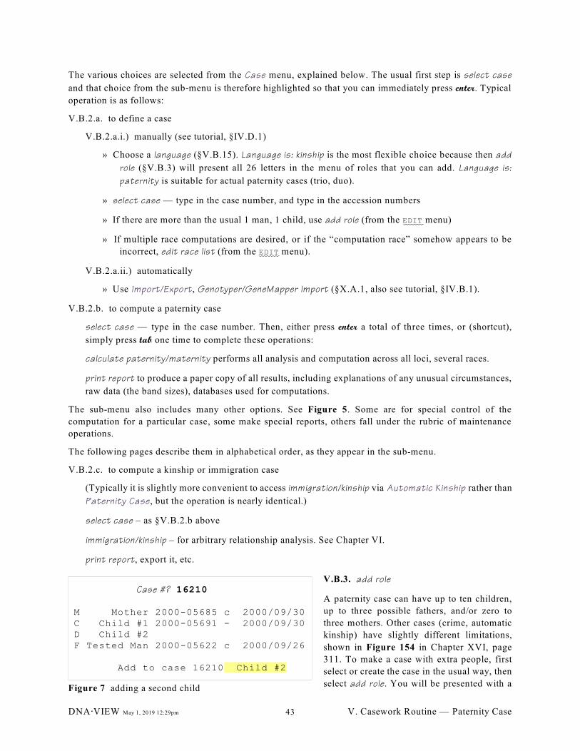
Case #? 16210
M Mother 2000-05685 c 2000/09/30C Child #1 2000-05691 - 2000/09/30D Child #2F Tested Man 2000-05622 c 2000/09/26
Add to case 16210 Child #2
Figure 7 adding a second child
The various choices are selected from the Case menu, explained below. The usual first step is select case
and that choice from the sub-menu is therefore highlighted so that you can immediately press enter. Typical
operation is as follows:
V.B.2.a. to define a case
V.B.2.a.i.) manually (see tutorial, §IV.D.1)
» Choose a language (§V.B.15). Language is: kinship is the most flexible choice because then add
role (§V.B.3) will present all 26 letters in the menu of roles that you can add. Language is:
paternity is suitable for actual paternity cases (trio, duo).
» select case — type in the case number, and type in the accession numbers
» If there are more than the usual 1 man, 1 child, use add role (from the EDIT menu)
» If multiple race computations are desired, or if the “computation race” somehow appears to be
incorrect, edit race list (from the EDIT menu).
V.B.2.a.ii.) automatically
» Use Import/Export, Genotyper/GeneMapper Import (§X.A.1, also see tutorial, §IV.B.1).
V.B.2.b. to compute a paternity case
select case — type in the case number. Then, either press enter a total of three times, or (shortcut),
simply press tab one time to complete these operations:
calculate paternity/maternity performs all analysis and computation across all loci, several races.
print report to produce a paper copy of all results, including explanations of any unusual circumstances,
raw data (the band sizes), databases used for computations.
The sub-menu also includes many other options. See Figure 5. Some are for special control of the
computation for a particular case, some make special reports, others fall under the rubric of maintenance
operations.
The following pages describe them in alphabetical order, as they appear in the sub-menu.
V.B.2.c. to compute a kinship or immigration case
(Typically it is slightly more convenient to access immigration/kinship via Automatic Kinship rather than
Paternity Case, but the operation is nearly identical.)
select case – as §V.B.2.b above
immigration/kinship – for arbitrary relationship analysis. See Chapter VI.
print report, export it, etc.
V.B.3. add role
A paternity case can have up to ten children,
up to three possible fathers, and/or zero to
three mothers. Other cases (crime, automatic
kinship) have slightly different limitations,
shown in Figure 154 in Chapter XVI, page
311. To make a case with extra people, first
select or create the case in the usual way, then
select add role. You will be presented with a
DNA@VIEW May 1, 2019 12:29pm V. Casework Routine — Paternity Case43
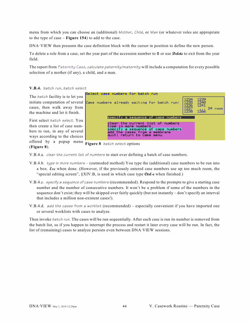
Figure 8 batch select options
menu from which you can choose an (additional) Mother, Child, or Man (or whatever roles are appropriate
to the type of case – Figure 154) to add to the case.
DNA·VIEW then presents the case definition block with the cursor in position to define the new person.
To delete a role from a case, set the year part of the accession number to 0 or use Delete to exit from the year
field.
The report from Paternity Case, calculate paternity/maternity will include a computation for every possible
selection of a mother (if any), a child, and a man.
V.B.4. batch run, batch select
The batch facility is to let you
initiate computation of several
cases, then walk away from
the machine and let it finish.
First select batch select. You
then create a list of case num-
bers to run, in any of several
ways according to the choices
offered by a popup menu
(Figure 8).
V.B.4.a. clear the current list of numbers to start over defining a batch of case numbers.
V.B.4.b. type in more numbers – (outmoded method) You type the (additional) case numbers to be run into
a box. Esc when done. (However, if the previously entered case numbers use up too much room, the
“special editing screen”, §XIV.B, is used in which case type Ctrl-e when finished.)
V.B.4.c. specify a sequence of case numbers (recommended). Respond to the prompts to give a starting case
number and the number of consecutive numbers. It won’t be a problem if some of the numbers in the
sequence don’t exist; they will be skipped over fairly quickly (but not instantly – don’t specify an interval
that includes a million non-existent cases!).
V.B.4.d. add the cases from a worklist (recommended) – especially convenient if you have imported one
or several worklists with cases to analyze.
Then invoke batch run. The cases will be run sequentially. After each case is run its number is removed from
the batch list, so if you happen to interrupt the process and restart it later every case will be run. In fact, the
list of (remaining) cases to analyze persists even between DNAAVIEW sessions.
DNA@VIEW May 1, 2019 12:29pm V. Casework Routine — Paternity Case44
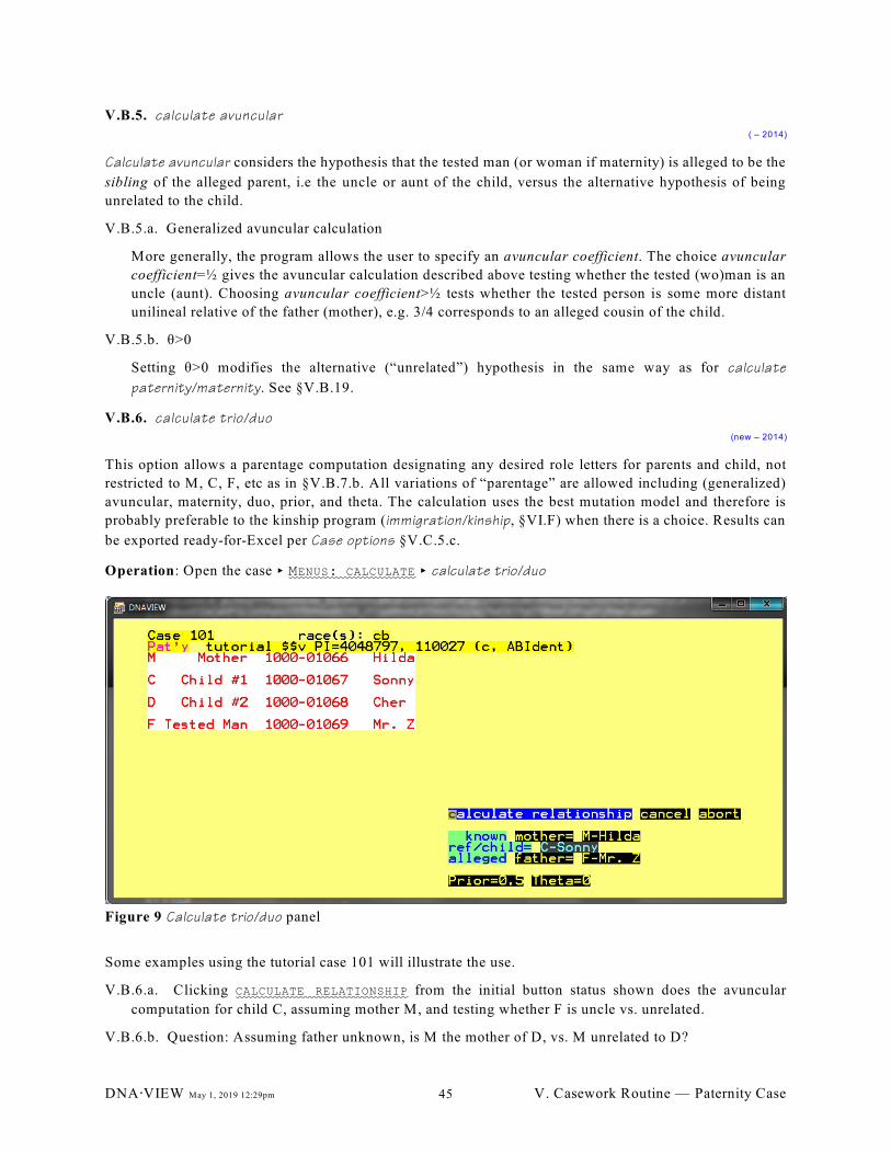
V.B.5. calculate avuncular( – 2014)
Calculate avuncular considers the hypothesis that the tested man (or woman if maternity) is alleged to be the
sibling of the alleged parent, i.e the uncle or aunt of the child, versus the alternative hypothesis of being
unrelated to the child.
V.B.5.a. Generalized avuncular calculation
More generally, the program allows the user to specify an avuncular coefficient. The choice avuncular
coefficient=½ gives the avuncular calculation described above testing whether the tested (wo)man is an
uncle (aunt). Choosing avuncular coefficient>½ tests whether the tested person is some more distant
unilineal relative of the father (mother), e.g. 3/4 corresponds to an alleged cousin of the child.
V.B.5.b. è>0
Setting è>0 modifies the alternative (“unrelated”) hypothesis in the same way as for calculate
paternity/maternity. See §V.B.19.
V.B.6. calculate trio/duo(new – 2014)
This option allows a parentage computation designating any desired role letters for parents and child, not
restricted to M, C, F, etc as in §V.B.7.b. All variations of “parentage” are allowed including (generalized)
avuncular, maternity, duo, prior, and theta. The calculation uses the best mutation model and therefore is
probably preferable to the kinship program (immigration/kinship, §VI.F) when there is a choice. Results can
be exported ready-for-Excel per Case options §V.C.5.c.
Operation: Open the case < MENUS: CALCULATE < calculate trio/duo
Some examples using the tutorial case 101 will illustrate the use.
V.B.6.a. Clicking CALCULATE RELATIONSHIP from the initial button status shown does the avuncular
computation for child C, assuming mother M, and testing whether F is uncle vs. unrelated.
V.B.6.b. Question: Assuming father unknown, is M the mother of D, vs. M unrelated to D?
Figure 9 Calculate trio/duo panel
DNA@VIEW May 1, 2019 12:29pm V. Casework Routine — Paternity Case45
Solution: Click MOTHER= and from the popup menu select language: maternity. (The case switches to
Mat’y and the button changes to FATHER=. Also, the last button changes to F-HILDA.)
Click the button after FATHER= and from the popup click (NONE).
Click REF/CHILD=... and select D-Cher
Click ALLEGED UNCLE/AUNT/GPARENT= and choose mother.
Leave the last button as F-HILDA.
Enter to CALCULATE RELATIONSHIP.
V.B.6.c. Question: Can C be the father of D? Assume prior probability=2% and compare with the alternative
of a random father slightly (è=0.01) related to D.
Solution: Restore (if necessary) KNOWN FATHER= to MOTHER=. Set the next button to (NONE).
After REF/CHILD=, put D-CHER.
After ALLEGED, put FATHER=, then C=SONNY.
Click PRIOR and set to 0.02. Click THETA and set to 0.01.
Enter to CALCULATE RELATIONSHIP.
DNA@VIEW May 1, 2019 12:29pm V. Casework Routine — Paternity Case46
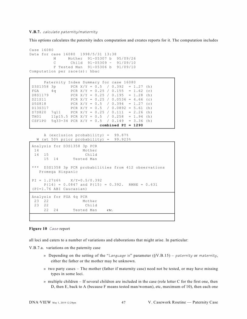
Case 16080Data for case 16080 1998/5/31 13:38 M Mother 91-05307 b 95/09/26 C Child 91-05309 - 91/09/10 F Tested Man 91-05306 b 91/09/10Computation per race(s): hbac
Paternity Index Summary for case 16080D3S1358 3p PCR X/Y = 0.5 / 0.392 = 1.27 (h)FGA 4q PCR X/Y = 0.25 / 0.155 = 1.62 (c)D8S1179 PCR X/Y = 0.25 / 0.195 = 1.28 (h)D21S11 PCR X/Y = 0.25 / 0.0536 = 4.66 (c)D5S818 PCR X/Y = 0.5 / 0.394 = 1.27 (c)D13S317 PCR X/Y = 0.5 / 0.0892 = 5.61 (h)D7S820 7q11 PCR X/Y = 0.25 / 0.111 = 2.26 (h)TH01 11p15.5 PCR X/Y = 0.5 / 0.258 = 1.94 (h)CSF1PO 5q33-34 PCR X/Y = 0.5 / 0.149 = 3.36 (h) combined PI = 1290
A (exclusion probability) = 99.87% W (at 50% prior probability) = 99.923%
Analysis for D3S1358 3p PCR 14 Mother 14 15 Child 15 14 Tested Man
*** D3S1358 3p PCR probabilities from 412 observations Promega Hispanic
PI = 1.27±6% X/Y=0.5/0.392 P{14} = 0.0847 and P{15} = 0.392. RMNE = 0.631(PI=1.76 ABI Caucasian)
Analysis for FGA 4q PCR 23 22 Mother 23 22 Child
22 24 Tested Man etc.
Figure 10 Case report
V.B.7. calculate paternity/maternity
This options calculates the paternity index computation and creates reports for it. The computation includes
all loci and caters to a number of variations and elaborations that might arise. In particular:
V.B.7.a. variations on the paternity case
» Depending on the setting of the “Language is” parameter (§V.B.15) – paternity or maternity,
either the father or the mother may be unknown.
» two party cases – The mother (father if maternity case) need not be tested, or may have missing
types in some loci.
» multiple children – If several children are included in the case (role letter C for the first one, then
D, then E, back to A (because F means tested man/woman), etc, maximum of 10), then each one
DNA@VIEW May 1, 2019 12:29pm V. Casework Routine — Paternity Case47
is computed as a separate trio. If you would like to make a computation that takes the several
children into account simultaneously, use Kinship, Chapter VI).
» multiple tested men/women – Similarly, more than one suspected father (or suspected mother if
maternity, or for that matter, though it is not very likely, more than one presumed mother/father)
may be included in the case – using role letters F for the first one, then G, then H – and every
different man-woman-child combination is computed as a separate trio.
V.B.7.a.i.) Mutation possibilities (§XIII.C) are computed automatically (§V.C.3). A mutation
calculation is indicated by a code on the Case report (Figure 10). The symbol ì (mutation) indicates
that a mutation calculation has rescued a nominally inconsistent pattern such as child=18, tested
man=15 19 from what would otherwise be PI=0:
VWA X/Y = 1/2350 / 0.113 = 1/266 (c) ì
A * symbol means that the pattern is consistent, but the parameter of §V.C.3.f is set so small that
a mutation explanation is also included for accuracy. For example if the paternal allele is rare the
random man computation might take into account not only a random sperm with the rare allele
but also a random sperm mutated from a neighboring common allele.
» Null allele (or inheritable primer hybridization failure) possibilities are computed automatically
(§XIII.B.5).
V.B.7.b. Role letters and paternity cases
For the purpose of this option only, the role letters – M, C, F, etc – have special computational
significance. In the simple trio paternity case, the M is the mother, F the alleged father, and C the child.
» For maternity cases or those with extra people, please look at the role letter chart, Figure 154,
page 311.
» For maternity cases specifically be sure to note that M means father! (§XVI.A.1.a)
V.B.7.c. multiple or various race computation (§V.C.6.a)
The menu option calculate paternity/maternity collects all the available measurements relevant to the case.
The data is condensed into one size measurement per individual per locus by the averaging algorithm
described in §XIII.F.
Analysis then proceeds
V.B.7.d. trio-by-trio. If there are extra men and/or children then each combination of man and child is treated
as an independent case. For example a case with two men and three children is calculated as 6 trio cases.
It may be that there is no maternal data; the man-child duo is then considered as a “trio.”
For each trio, the analysis is:
V.B.7.e. locus-by-locus. For each locus, the program decides on the pattern of possibly matching alleles
among the parties of the trio, then makes a PI calculation.
V.B.7.e.i.) Matching patterns are shown in boxes for the example case of Figure 10 The allele measure-
ments (averaged over multiple assays in the case of RFLP) are presented in staggered rows, as shown
in the boxes in Figure 10. The rows labeled mother, child, tested man, and man & child, and show
the allele sizes of each person or combination. The rows are staggered to indicate the apparent
sharing of alleles through inheritance.
V.B.7.e.ii.) Race-by-race
V.B.7.e.iii.) Choice of race
DNA@VIEW May 1, 2019 12:29pm V. Casework Routine — Paternity Case48
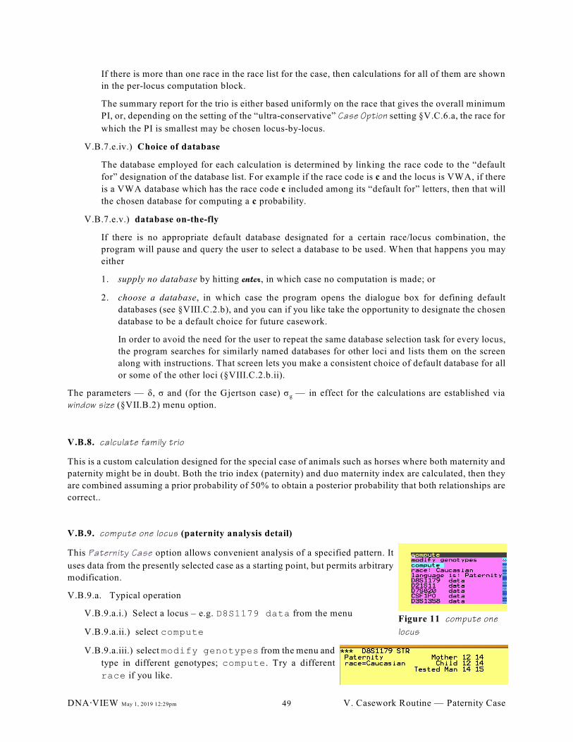
Figure 11 compute one
locus
If there is more than one race in the race list for the case, then calculations for all of them are shown
in the per-locus computation block.
The summary report for the trio is either based uniformly on the race that gives the overall minimum
PI, or, depending on the setting of the “ultra-conservative” Case Option setting §V.C.6.a, the race for
which the PI is smallest may be chosen locus-by-locus.
V.B.7.e.iv.) Choice of database
The database employed for each calculation is determined by linking the race code to the “default
for” designation of the database list. For example if the race code is c and the locus is VWA, if there
is a VWA database which has the race code c included among its “default for” letters, then that will
the chosen database for computing a c probability.
V.B.7.e.v.) database on-the-fly
If there is no appropriate default database designated for a certain race/locus combination, the
program will pause and query the user to select a database to be used. When that happens you may
either
1. supply no database by hitting enter, in which case no computation is made; or
2. choose a database, in which case the program opens the dialogue box for defining default
databases (see §VIII.C.2.b), and you can if you like take the opportunity to designate the chosen
database to be a default choice for future casework.
In order to avoid the need for the user to repeat the same database selection task for every locus,
the program searches for similarly named databases for other loci and lists them on the screen
along with instructions. That screen lets you make a consistent choice of default database for all
or some of the other loci (§VIII.C.2.b.ii).
gThe parameters — ä, ó and (for the Gjertson case) ó — in effect for the calculations are established via
window size (§VII.B.2) menu option.
V.B.8. calculate family trio
This is a custom calculation designed for the special case of animals such as horses where both maternity and
paternity might be in doubt. Both the trio index (paternity) and duo maternity index are calculated, then they
are combined assuming a prior probability of 50% to obtain a posterior probability that both relationships are
correct..
V.B.9. compute one locus (paternity analysis detail)
This Paternity Case option allows convenient analysis of a specified pattern. It
uses data from the presently selected case as a starting point, but permits arbitrary
modification.
V.B.9.a. Typical operation
V.B.9.a.i.) Select a locus – e.g. D8S1179 data from the menu
V.B.9.a.ii.) select compute
V.B.9.a.iii.) select modify genotypes from the menu and
type in different genotypes; compute. Try a different
race if you like.
DNA@VIEW May 1, 2019 12:29pm V. Casework Routine — Paternity Case49
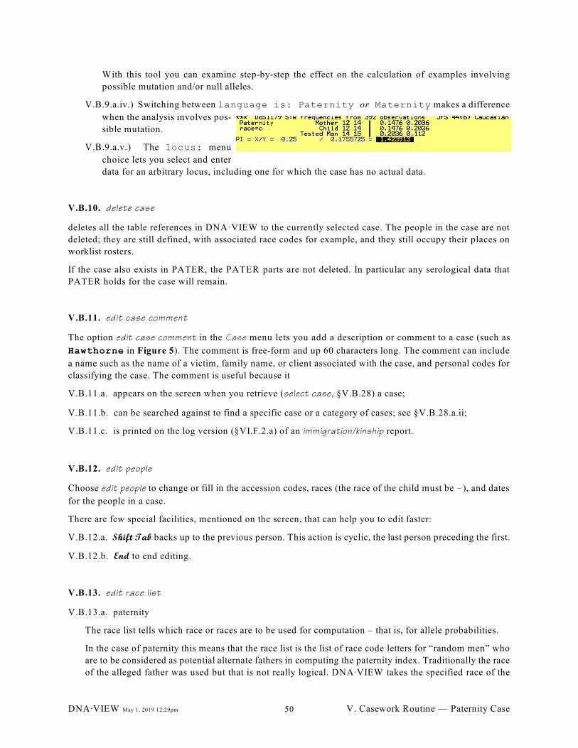
With this tool you can examine step-by-step the effect on the calculation of examples involving
possible mutation and/or null alleles.
V.B.9.a.iv.) Switching between language is: Paternity or Maternity makes a difference
when the analysis involves pos-
sible mutation.
V.B.9.a.v.) The locus: menu
choice lets you select and enter
data for an arbitrary locus, including one for which the case has no actual data.
V.B.10. delete case
deletes all the table references in DNA·VIEW to the currently selected case. The people in the case are not
deleted; they are still defined, with associated race codes for example, and they still occupy their places on
worklist rosters.
If the case also exists in PATER, the PATER parts are not deleted. In particular any serological data that
PATER holds for the case will remain.
V.B.11. edit case comment
The option edit case comment in the Case menu lets you add a description or comment to a case (such as
Hawthorne in Figure 5). The comment is free-form and up 60 characters long. The comment can include
a name such as the name of a victim, family name, or client associated with the case, and personal codes for
classifying the case. The comment is useful because it
V.B.11.a. appears on the screen when you retrieve (select case, §V.B.28) a case;
V.B.11.b. can be searched against to find a specific case or a category of cases; see §V.B.28.a.ii;
V.B.11.c. is printed on the log version (§VI.F.2.a) of an immigration/kinship report.
V.B.12. edit people
Choose edit people to change or fill in the accession codes, races (the race of the child must be !), and dates
for the people in a case.
There are few special facilities, mentioned on the screen, that can help you to edit faster:
V.B.12.a. Shift Tab backs up to the previous person. This action is cyclic, the last person preceding the first.
V.B.12.b. End to end editing.
V.B.13. edit race list
V.B.13.a. paternity
The race list tells which race or races are to be used for computation – that is, for allele probabilities.
In the case of paternity this means that the race list is the list of race code letters for “random men” who
are to be considered as potential alternate fathers in computing the paternity index. Traditionally the race
of the alleged father was used but that is not really logical. DNAAVIEW takes the specified race of the
DNA@VIEW May 1, 2019 12:29pm V. Casework Routine — Paternity Case50
alleged father to seed the race list, i.e. as a default for the computation race, but since the user can edit
the race list there are conceptually two different roles that race can play in a case:
» The race list specifies the “computation race” or races.
» The race of the alleged father is merely his “databasing race” – in case his DNA is eventually
included in allele frequency databases.
By using edit race list, that letter may be changed to another letter, or to a list of several letters. Note that
once this is done, the race of the alleged father no longer plays any role in the paternity index
computation.
When there are several race list letters, the calculate paternity/maternity option will attempt to make a
computation for each letter for each probe/locus. The smallest PI thus obtained, locus by locus, is the one
used for the PI summary and the cumulative PI in the case.
V.B.13.b. kinship
The first race on the list is the one initially selected for kinship (immigration/kinship, Chapter VI)
computations and simulations.
The race list is the list of alternate computations that are made by the Calculate & report LRs, [all] races
(§VI.F.2) option and the list of races included in the Next race from: (§VI.F.7.h) option.
V.B.14. export case
This option creates a text file that contains the essential data of the case – names, roles, and genotypes. The
text file format is like the ABI Genotyper “allele table,” so that it can be imported into DNAAVIEW using the
Import/export < Genotyper import option (§X.A.1).
This is therefore a convenient way to communicate a case to another person, especially another user of DNAA
VIEW, who can simply use Import the file and recreate the same case. The people are designated in the
“Sample Info” column using the role-within-case format (see Figure 123, page236) By default the exported
case number is the original case number, but you are given an opportunity to specify a different case number
instead.
V.B.14.a. Creating a case from a simulation
The Kinship simulation (§VI.G) menu includes an option to export in the same way. Therefore it is
possible to generate simulated profiles according to a specified relationship scenario, export the simulated
types, then import them in order to create a practice case.
V.B.15. immigration/kinship
Use: Relationship calculations for any non-standard situation.
This sub-option of Automatic Kinship/Paternity /Automatic mixture is a link to Kinship (Chapter VI).
Immigration cases is just one application — it can equally be used for any kinship problem including
paternity, inheritance, missing person, etc.
For instance, you can type the kinship scenario definition
C : M + F/?
to immigration/kinship and thereby obtain approximately the same result as the normal trio analysis via
calculate paternity/maternity §V.B.7). However, you can also enter any other kinship formula, and thereby
quickly and automatically investigate other kinds of relationship.
DNA@VIEW May 1, 2019 12:29pm V. Casework Routine — Paternity Case51
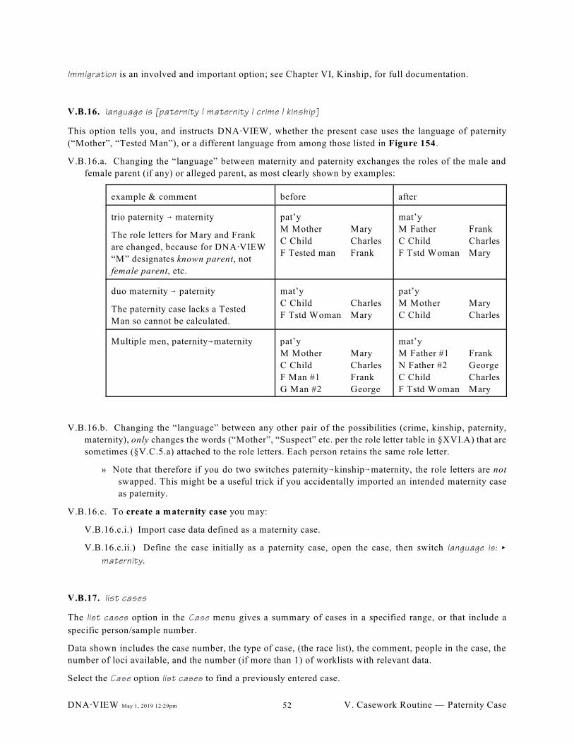
Immigration is an involved and important option; see Chapter VI, Kinship, for full documentation.
V.B.16. language is [paternity | maternity | crime | kinship]
This option tells you, and instructs DNA@VIEW, whether the present case uses the language of paternity
(“Mother”, “Tested Man”), or a different language from among those listed in Figure 154.
V.B.16.a. Changing the “language” between maternity and paternity exchanges the roles of the male and
female parent (if any) or alleged parent, as most clearly shown by examples:
example & comment before after
trio paternity 6 maternity
The role letters for Mary and Frank
are changed, because for DNA@VIEW
“M” designates known parent, not
female parent, etc.
pat’y
M Mother Mary
C Child Charles
F Tested man Frank
mat’y
M Father Frank
C Child Charles
F Tstd Woman Mary
duo maternity 6 paternity
The paternity case lacks a Tested
Man so cannot be calculated.
mat’y
C Child Charles
F Tstd Woman Mary
pat’y
M Mother Mary
C Child Charles
Multiple men, paternity6maternity pat’y
M Mother Mary
C Child Charles
F Man #1 Frank
G Man #2 George
mat’y
M Father #1 Frank
N Father #2 George
C Child Charles
F Tstd Woman Mary
V.B.16.b. Changing the “language” between any other pair of the possibilities (crime, kinship, paternity,
maternity), only changes the words (“Mother”, “Suspect” etc. per the role letter table in §XVI.A) that are
sometimes (§V.C.5.a) attached to the role letters. Each person retains the same role letter.
» Note that therefore if you do two switches paternity6kinship6maternity, the role letters are not
swapped. This might be a useful trick if you accidentally imported an intended maternity case
as paternity.
V.B.16.c. To create a maternity case you may:
V.B.16.c.i.) Import case data defined as a maternity case.
V.B.16.c.ii.) Define the case initially as a paternity case, open the case, then switch language is: <
maternity.
V.B.17. list cases
The list cases option in the Case menu gives a summary of cases in a specified range, or that include a
specific person/sample number.
Data shown includes the case number, the type of case, (the race list), the comment, people in the case, the
number of loci available, and the number (if more than 1) of worklists with relevant data.
Select the Case option list cases to find a previously entered case.
DNA@VIEW May 1, 2019 12:29pm V. Casework Routine — Paternity Case52
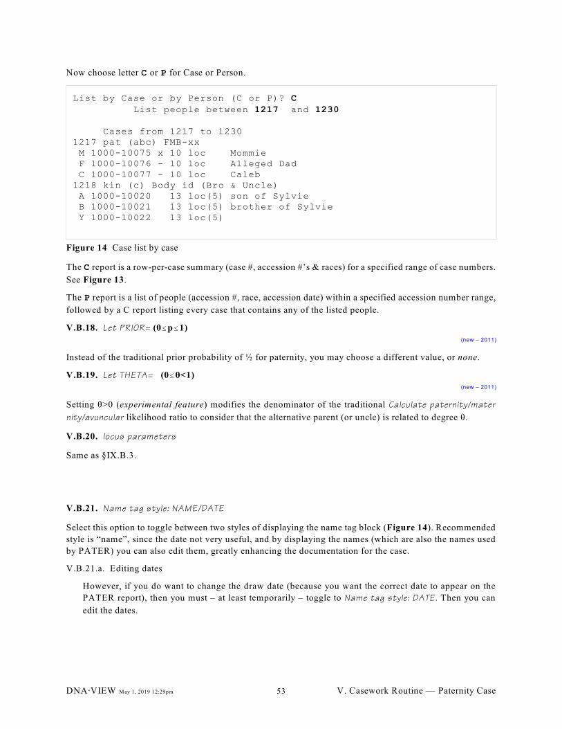
List by Case or by Person (C or P)? C List people between 1217 and 1230
Cases from 1217 to 12301217 pat (abc) FMB-xx M 1000-10075 x 10 loc Mommie F 1000-10076 - 10 loc Alleged Dad C 1000-10077 - 10 loc Caleb1218 kin (c) Body id (Bro & Uncle) A 1000-10020 13 loc(5) son of Sylvie B 1000-10021 13 loc(5) brother of Sylvie Y 1000-10022 13 loc(5)
Figure 14 Case list by case
Now choose letter C or P for Case or Person.
The C report is a row-per-case summary (case #, accession #’s & races) for a specified range of case numbers.
See Figure 13.
The P report is a list of people (accession #, race, accession date) within a specified accession number range,
followed by a C report listing every case that contains any of the listed people.
V.B.18. Let PRIOR= (0#p#1)(new – 2011)
Instead of the traditional prior probability of ½ for paternity, you may choose a different value, or none.
V.B.19. Let THETA= (0#è<1)(new – 2011)
Setting è>0 (experimental feature) modifies the denominator of the traditional Calculate paternity/mater
nity/avuncular likelihood ratio to consider that the alternative parent (or uncle) is related to degree è.
V.B.20. locus parameters
Same as §IX.B.3.
V.B.21. Name tag style: NAME/DATE
Select this option to toggle between two styles of displaying the name tag block (Figure 14). Recommended
style is “name”, since the date not very useful, and by displaying the names (which are also the names used
by PATER) you can also edit them, greatly enhancing the documentation for the case.
V.B.21.a. Editing dates
However, if you do want to change the draw date (because you want the correct date to appear on the
PATER report), then you must – at least temporarily – toggle to Name tag style: DATE. Then you can
edit the dates.
DNA@VIEW May 1, 2019 12:29pm V. Casework Routine — Paternity Case53
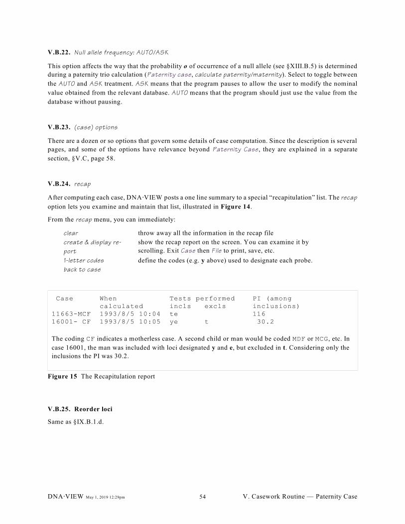
Case When Tests performed PI (among calculated incls excls inclusions)11663-MCF 1993/8/5 10:04 te 11616001- CF 1993/8/5 10:05 ye t 30.2
The coding CF indicates a motherless case. A second child or man would be coded MDF or MCG, etc. In
case 16001, the man was included with loci designated y and e, but excluded in t. Considering only the
inclusions the PI was 30.2.
Figure 15 The Recapitulation report
V.B.22. Null allele frequency: AUTO/ASK
This option affects the way that the probability o of occurrence of a null allele (see §XIII.B.5) is determined
during a paternity trio calculation (Paternity case, calculate paternity/maternity). Select to toggle between
the AUTO and ASK treatment. ASK means that the program pauses to allow the user to modify the nominal
value obtained from the relevant database. AUTO means that the program should just use the value from the
database without pausing.
V.B.23. (case) options
There are a dozen or so options that govern some details of case computation. Since the description is several
pages, and some of the options have relevance beyond Paternity Case , they are explained in a separate
section, §V.C, page 58.
V.B.24. recap
After computing each case, DNA@VIEW posts a one line summary to a special “recapitulation” list. The recap
option lets you examine and maintain that list, illustrated in Figure 14.
From the recap menu, you can immediately:
clear throw away all the information in the recap file
create & display re-
port
show the recap report on the screen. You can examine it by
scrolling. Exit Case then File to print, save, etc.
1-letter codes define the codes (e.g. y above) used to designate each probe.
back to case
V.B.25. Reorder loci
Same as §IX.B.1.d.
DNA@VIEW May 1, 2019 12:29pm V. Casework Routine — Paternity Case54
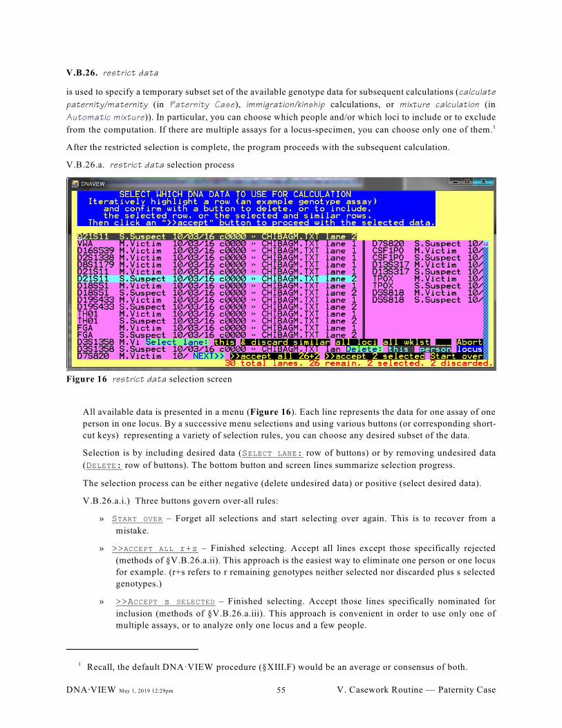
Figure 16 restrict data selection screen
V.B.26. restrict data
is used to specify a temporary subset set of the available genotype data for subsequent calculations (calculate
paternity/maternity (in Paternity Case), immigration/kinship calculations, or mixture calculation (in
Automatic mixture)). In particular, you can choose which people and/or which loci to include or to exclude
from the computation. If there are multiple assays for a locus-specimen, you can choose only one of them.1
After the restricted selection is complete, the program proceeds with the subsequent calculation.
V.B.26.a. restrict data selection process
All available data is presented in a menu (Figure 16). Each line represents the data for one assay of one
person in one locus. By a successive menu selections and using various buttons (or corresponding short-
cut keys) representing a variety of selection rules, you can choose any desired subset of the data.
Selection is by including desired data (SELECT LANE: row of buttons) or by removing undesired data
(DELETE: row of buttons). The bottom button and screen lines summarize selection progress.
The selection process can be either negative (delete undesired data) or positive (select desired data).
V.B.26.a.i.) Three buttons govern over-all rules:
» START OVER – Forget all selections and start selecting over again. This is to recover from a
mistake.
» >>ACCEPT ALL r+s – Finished selecting. Accept all lines except those specifically rejected
(methods of §V.B.26.a.ii). This approach is the easiest way to eliminate one person or one locus
for example. (r+s refers to r remaining genotypes neither selected nor discarded plus s selected
genotypes.)
» >>ACCEPT s SELECTED – Finished selecting. Accept those lines specifically nominated for
inclusion (methods of §V.B.26.a.iii). This approach is convenient in order to use only one of
multiple assays, or to analyze only one locus and a few people.
Recall, the default DNA·VIEW procedure (§XIII.F) would be an average or consensus of both.1
DNA@VIEW May 1, 2019 12:29pm V. Casework Routine — Paternity Case55
The remaining buttons apply after first moving the bounce-bar highlight to a particular menu item. They
are logically divided into two categories:
V.B.26.a.ii.) Rejection buttons, preliminary to >>ACCEPT ALL ...
» DELETE: THIS – omit this assay of a person/locus.
» DELETE: PERSON – omit this person (i.e. this line and also other lines with the same role letter).
» DELETE: LOCUS – omit this locus (i.e. this line and also other lines with the same locus).
V.B.26.a.iii.) Selecting buttons, preliminary to >>ACCEPT .. SELECTED
» SELECT LANE: THIS – include this person-locus genotype
» SELECT LANE: THIS & DISCARD SIMILAR – include only the highlighted assay of a
person/locus (removing any other assays for the same person/locus).
» SELECT LANE: ALL LOCI – include this line and also all other loci for the same person/lane/roster.
» SELECT LANE: ALL WKLST – include this line and also all lines (genotypes) from the same worklist
so long as the genotype occurs just once. (For example do not include a person-locus
combination which occurs in two different lanes).
V.B.27. review/print report
Open the Case report long version (In addition to the key information that is shown in Figure 10, it also
contains information about inconsistent readings and ignored data.) in a print-preview-like window (as
§V.K.3) for printing or saving.
V.B.28. select case
Choose select case to change the current default case
number, or to initiate a new case. The case number
selection dialogue may also occur in other contexts (e.g.
§V.J.3.d).
You may simply type in a number. Or, there are various tricks (§V.B.28.a) to find a case or help type. If the
case number is already on file, identification data is presented for mother, child, and tested man as shown in
Figure 5, page 41.
If the case number is not already on file, an empty case matrix is presented on the screen and you will be
asked to enter (per §V.B.12) the people of the new case.
V.B.28.a. Selecting tricks (revised – 2011)
A number of shortcuts and other aids are available to make it easier to find the right case number.
V.B.28.a.i.) RECENT for recently visited or popular cases.
This key pops up case-selection-menu of recently-used or often-used case numbers.
The parenthetical numbers following the case number are the number of times that the case has been
selected, among the most recent 500 selections.
» The Recent box includes WORKLIST button, which allows selection of a worklist whose cases are
then added to the recent list.
DNA@VIEW May 1, 2019 12:29pm V. Casework Routine — Paternity Case56
Notes:
» The cases from a just-used worklist will already be included in the list per §V.B.28.a.i. In
particular, if you have just done a Genotyper Import for example, then the new cases are
automatically in the recent or popular case list.
» Dashes instead of a parenthetical number after the case means zero previous selections, and the
case is from the selected worklist.
» Such dash-denoted cases are put at the top of the list. This makes it convenient to successively
analyze all the cases of a worklist. You can simply pick the top one, analyze it, then select the
new top one, and continue in this manner until there are no more dashes.
V.B.28.a.ii.) SEARCH – and optionally open a case – by case number or case comments (§V.B.11) which
are displayed in a popup window. This facility becomes a powerful open-ended feature by judicious
use of case comments thanks to the context searching (§XIV.A.2.a.iii) property of DNA@VIEW
menus.
If the comment contains the name, typing the name at this menu automatically finds the correspond-
ing case.
Further it is convenient to search for all the cases with a particular code or set of codes embedded in
the comment. Recommended and suggested codes include
>> Screen disaster matches can recognize this as a completed or
otherwise presently inactive case and sort it to the end.$v Case used for validation
$r or >>$r Case currently under review{C:M+Fa/?{Fa,M: ?+?} kinship scenario for the case (example)
V.B.28.a.iii.) prefixing a year number. Type the sequence part of the case such as 987 then click one
of the YEAR: buttons to prefix digits representing THIS, LAST, or NEXT year. The number of year
digits, and whether the sequence part is padded with leading 0s, depends on the Case # format
(§IX.F.2).
V.B.28.a.iv.) NEXT AVAILABLE NUMBER – First type a positive integer (a possible case number), then click
to obtain an unused case number.
V.B.29. simulation
Same as §VI.G.
V.B.30. parentage test examples
This is a validation option to run a variety of paternity calculations, comparing the results against canned
results. The main purpose is to test DNA@VIEW versions before release.
DNA@VIEW May 1, 2019 12:29pm V. Casework Routine — Paternity Case57
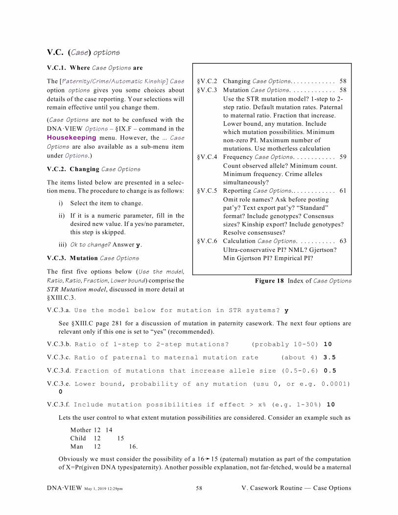
§V.C.2 Changing Case Options. . . . . . . . . . . . . 58
§V.C.3 Mutation Case Options. . . . . . . . . . . . . 58
Use the STR mutation model? 1-step to 2-
step ratio. Default mutation rates. Paternal
to maternal ratio. Fraction that increase.
Lower bound, any mutation. Include
which mutation possibilities. Minimum
non-zero PI. Maximum number of
mutations. Use motherless calculation
§V.C.4 Frequency Case Options. . . . . . . . . . . . 59
Count observed allele? Minimum count.
Minimum frequency. Crime alleles
simultaneously?
§V.C.5 Reporting Case Options. . . . . . . . . . . . . 61
Omit role names? Ask before posting
pat’y? Text export pat’y? “Standard”
format? Include genotypes? Consensus
sizes? Kinship export? Include genotypes?
Resolve consensuses?
§V.C.6 Calculation Case Options. . . . . . . . . . . 63
Ultra-conservative PI? NML? Gjertson?
Min Gjertson PI? Empirical PI?
Figure 18 Index of Case Options
V.C. (Case) options
V.C.1. Where Case Options are
The [Paternity/Crime/Automatic Kinship] Case
option options gives you some choices about
details of the case reporting. Your selections will
remain effective until you change them.
(Case Options are not to be confused with the
DNA·VIEW Options – §IX.F – command in the
Housekeeping menu. However, the ... Case
Options are also available as a sub-menu item
under Options.)
V.C.2. Changing Case Options
The items listed below are presented in a selec-
tion menu. The procedure to change is as follows:
i) Select the item to change.
ii) If it is a numeric parameter, fill in the
desired new value. If a yes/no parameter,
this step is skipped.
iii) Ok to change? Answer y.
V.C.3. Mutation Case Options
The first five options below (Use the model,
Ratio, Ratio, Fraction, Lower bound) comprise the
STR Mutation model, discussed in more detail at
§XIII.C.3.
V.C.3.a. Use the model below for mutation in STR systems? y
See §XIII.C page 281 for a discussion of mutation in paternity casework. The next four options are
relevant only if this one is set to “yes” (recommended).
V.C.3.b. Ratio of 1-step to 2-step mutations? (probably 10-50) 10
V.C.3.c. Ratio of paternal to maternal mutation rate (about 4) 3.5
V.C.3.d. Fraction of mutations that increase allele size (0.5-0.6) 0.5
V.C.3.e. Lower bound, probability of any mutation (usu 0, or e.g. 0.0001)0
V.C.3.f. Include mutation possibilities if effect > x% (e.g. 1-30%) 10
Lets the user control to what extent mutation possibilities are considered. Consider an example such as
Mother 12 14
Child 12 15
Man 12 16.
Obviously we must consider the possibility of a 16ý15 (paternal) mutation as part of the computation
of X=Pr(given DNA types|paternity). Another possible explanation, not far-fetched, would be a maternal
DNA@VIEW May 1, 2019 12:29pm V. Casework Routine — Case Options58
14ý15 mutation with the man contributing the 12. A computation of X should probably include both of
these possibilities.
There are further theoretically possible explanations as well, such as with two mutations and mutation
of 12ý15. Including all of these in the computation would introduce complexity – difficulty in verifying
the computation – with no worthwhile gain in accuracy. It seems better to leave trivial terms off.
The mechanism implemented is to give the user the choice of omitting any terms that would affect the
answer by less than a user-chosen percentage.
V.C.3.g. Default STR mutation rate (if no locus-specific) (%; recommend
0.28%).(new – 2014) The typical mutation rate for a polymorphic forensic STR locus is 1/350 or 0.28%
hence the recommendation which is used for any STR locus whose locus-specific rate (§IX.B.3) is set
to 0. (Note – if this rate is 0 the non-STR value is substituted!)
V.C.3.h. Default non-STR mutation rate, e.g. SNP (logarithm, i.e. -8 for
10^-8).(new – 2014) A mutation rate often cited for single nucleotides is 10 , hence the recommendation.-8
V.C.3.i. Minimum PI – report PI as 0 if less than (0-1, reasonably 0.01)
See §XIII.C.1.c, page 281.
V.C.3.j. Max # inconsistencies for a parent (rec: 999; prefer “Min PI”) 999
See §XIII.C.1.c, page 281.
V.C.3.k. Use motherless calculation for loci with maternal exclusion?
(Recommend: no) n
Using STR systems and the STR mutation model (§V.C.3.a), no results in an excellent computation
properly taking into account the possibility of a maternal mutation. Yes means, if the mother is excluded,
ignore her and make the motherless calculation as if she were not typed in this locus.
V.C.4. Allele probability Case Options(revised – 2010)
There are various situations requiring an evidential matching probability, namely
the probability than a randomly selected allele (or haplotype) would match a given observed type.
The options in this section allows the user to select among various methods for making such a calculation.
V.C.4.a. Count observed allele in database how many times (recommend: 1)? 1
This option offers a coherent approach to the vexing problem of matching probabilities for rare alleles,
such as alleles that occur in a case but don’t exist in the database.
The recommendation is: any allele probability is calculated by adding the critical allele one extra time
to the database. If the present allele was observed k times in a database of N alleles, the probability is
(k+1)/(N+1). In particular for a never-before observed allele, the matching probability is 1/(N+1). See
§XIII.A.1.e for further discussion.
Why toss the new allele into the database? That’s easy — because we have seen it. The database should
be a representative sample; to ignore this most important observation would be to create bias. See
http://dna-view.com/AlleleProbability.htm for further discussion of this recommendation.
By setting the parameter (call it t) in this option to various values, the user can achieve various policies:
t=0 to retain the old (and industry standard) behavior, probability=k/N.
DNA@VIEW May 1, 2019 12:29pm V. Casework Routine — Case Options59
Also there may be circumstances where the suspect may be presumed already to be counted in the
database — a convicted offender database, for example.
t=1 recommended choice, following the above argument, probability=(k+1)/(N+1).
t=2 or more to give probabilities that are (conservatively) large.
Note a: This facility is therefore a clear improvement on and a preferred substitute for option §V.C.4.b.
Note b: See also the option §V.C.4.e below.
V.C.4.b. Minimum # of matching alleles to assume for probability calculations 1
This indirectly puts a cap (maximum value) on PI’s and other likelihood ratio computations. The default
and smallest allowable value is 1, so that PI is never infinite. Some statisticians like to use a larger value.
For example, a value of 3 guarantees than an allele probability will never be reported by DNA@VIEW as
rarer than 3/N (N=number of alleles in the database), which is 95% confident to be a conservative
estimate for the true frequency of an allele that was never before observed. (The astute reader will notice
a disconnect in confusing frequency and probability.)
The actual limit on PI implied by this parameter is proportional to the database size, and also depends on
the matching pattern (whether the man has 2 eligible alleles or one) in a given case.
V.C.4.c. Minimum frequency (recommend 0. prefer minimum count)
If you insist, you may set a minimum value for allele probabilities. Entering a probability f>1 is
interpreted as 1/f. That is, for a minimum probability of 1%, either enter 0.01, or enter 100.
If the motive for setting a floor is to take into account the effect of sampling variation, then the
appropriate frequency to choose should depend on sample size. In fact, it is very nearly proportional to
sample size, so a more sensible floor for frequencies is obtained by using option §V.C.4.b.
V.C.4.d. Y-haplotype LR model (recommend: 6 if rare)
There are three options for computation of Y-haplotype matching probability.
V.C.4.d.i.) count – the (augmented) sample frequency per §V.C.4.a is taken as the matching probability.
V.C.4.d.ii.) ê if rare (recommended) – For haplotypes never before seen, use the ê rule of Brenner
(2010), and see §VIII.F.5. For haplotypes already seen in the database, use the count rule.
V.C.4.d.iii.) ê always – Use the ê rule per Brenner (2010).
V.C.4.e. Calculate crime allele probabilities simultaneously? n
This option modifies the “(k+1)/(N+1)” allele probability computation behavior discussed above in
§V.C.4.a Count observed allele in database how many times.
I recommend not using this option (answer n) because the effect is complicated. It is offered only for
compatibility.
It applies only to crime casework — Mixture Calculator, DNA odds, DNA exclusion . For paternity and
immigration calculations, the probability of each allele is always computed independently of the others,
as described in §V.C.4.a.
If there are several alleles — s alleles — specified at a locus, a “(k+1)/N+s)” formula is used, which
represents including the alleles as part of the database for purposes of calculating the probability of each
one. See §XIII.A.1.e for the precise rules, and §XIII.A.1.e.iii for examples.
DNA@VIEW May 1, 2019 12:29pm V. Casework Routine — Case Options60
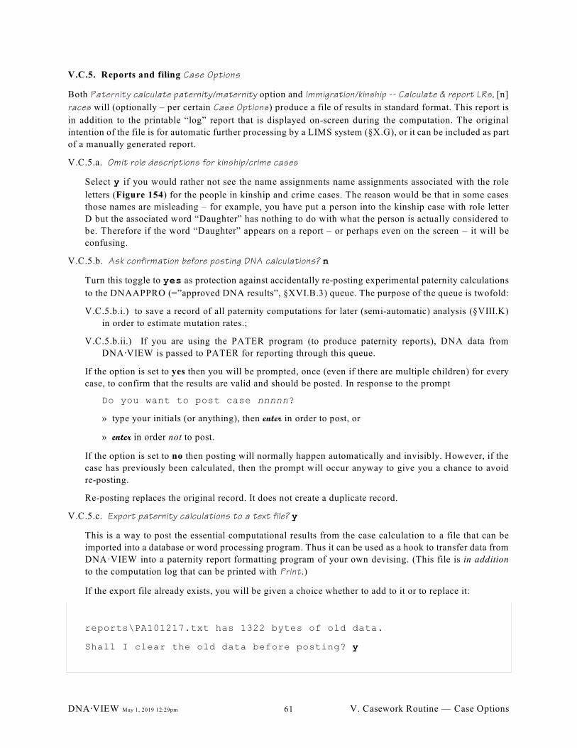
V.C.5. Reports and filing Case Options
Both Paternity calculate paternity/maternity option and Immigration/kinship -- Calculate & report LRs, [n]
races will (optionally – per certain Case Options) produce a file of results in standard format. This report is
in addition to the printable “log” report that is displayed on-screen during the computation. The original
intention of the file is for automatic further processing by a LIMS system (§X.G), or it can be included as part
of a manually generated report.
V.C.5.a. Omit role descriptions for kinship/crime cases
Select y if you would rather not see the name assignments name assignments associated with the role
letters (Figure 154) for the people in kinship and crime cases. The reason would be that in some cases
those names are misleading – for example, you have put a person into the kinship case with role letter
D but the associated word “Daughter” has nothing to do with what the person is actually considered to
be. Therefore if the word “Daughter” appears on a report – or perhaps even on the screen – it will be
confusing.
V.C.5.b. Ask confirmation before posting DNA calculations? n
Turn this toggle to yes as protection against accidentally re-posting experimental paternity calculations
to the DNAAPPRO (=”approved DNA results”, §XVI.B.3) queue. The purpose of the queue is twofold:
V.C.5.b.i.) to save a record of all paternity computations for later (semi-automatic) analysis (§VIII.K)
in order to estimate mutation rates.;
V.C.5.b.ii.) If you are using the PATER program (to produce paternity reports), DNA data from
DNA@VIEW is passed to PATER for reporting through this queue.
If the option is set to yes then you will be prompted, once (even if there are multiple children) for every
case, to confirm that the results are valid and should be posted. In response to the prompt
Do you want to post case nnnnn?
» type your initials (or anything), then enter in order to post, or
» enter in order not to post.
If the option is set to no then posting will normally happen automatically and invisibly. However, if the
case has previously been calculated, then the prompt will occur anyway to give you a chance to avoid
re-posting.
Re-posting replaces the original record. It does not create a duplicate record.
V.C.5.c. Export paternity calculations to a text file? y
This is a way to post the essential computational results from the case calculation to a file that can be
imported into a database or word processing program. Thus it can be used as a hook to transfer data from
DNA·VIEW into a paternity report formatting program of your own devising. (This file is in addition
to the computation log that can be printed with Print.)
If the export file already exists, you will be given a choice whether to add to it or to replace it:
reports\PA101217.txt has 1322 bytes of old data.
Shall I clear the old data before posting? y
DNA@VIEW May 1, 2019 12:29pm V. Casework Routine — Case Options61
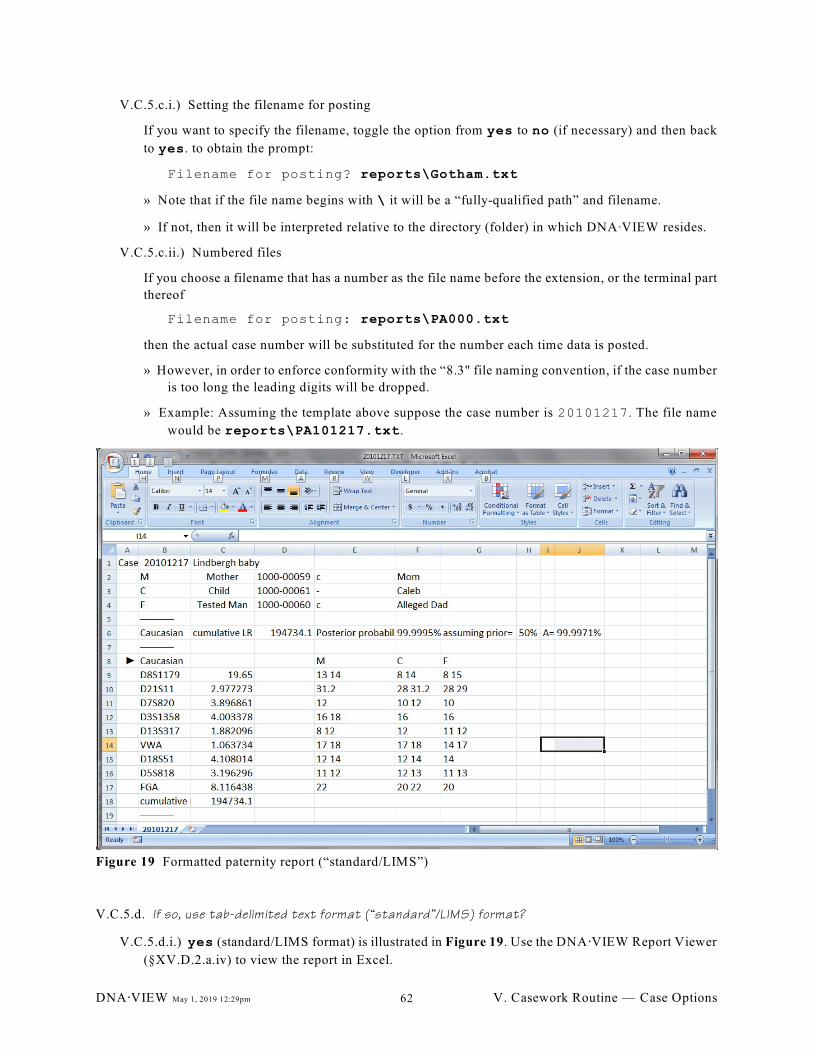
Figure 19 Formatted paternity report (“standard/LIMS”)
V.C.5.c.i.) Setting the filename for posting
If you want to specify the filename, toggle the option from yes to no (if necessary) and then back
to yes. to obtain the prompt:
Filename for posting? reports\Gotham.txt
» Note that if the file name begins with \ it will be a “fully-qualified path” and filename.
» If not, then it will be interpreted relative to the directory (folder) in which DNAAVIEW resides.
V.C.5.c.ii.) Numbered files
If you choose a filename that has a number as the file name before the extension, or the terminal part
thereof
Filename for posting: reports\PA000.txt
then the actual case number will be substituted for the number each time data is posted.
» However, in order to enforce conformity with the “8.3" file naming convention, if the case number
is too long the leading digits will be dropped.
» Example: Assuming the template above suppose the case number is 20101217. The file name
would be reports\PA101217.txt.
V.C.5.d. If so, use tab-delimited text format (“standard”/LIMS) format?
V.C.5.d.i.) yes (standard/LIMS format) is illustrated in Figure 19. Use the DNA@VIEW Report Viewer
(§XV.D.2.a.iv) to view the report in Excel.
DNA@VIEW May 1, 2019 12:29pm V. Casework Routine — Case Options62
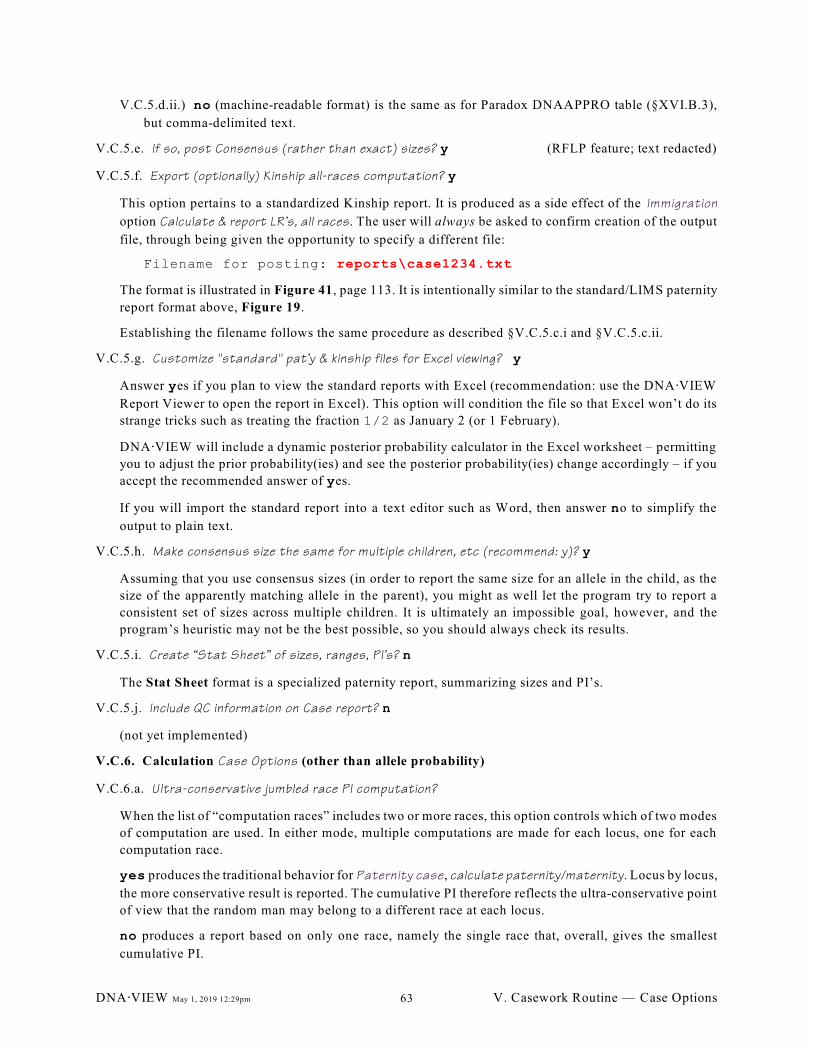
V.C.5.d.ii.) no (machine-readable format) is the same as for Paradox DNAAPPRO table (§XVI.B.3),
but comma-delimited text.
V.C.5.e. If so, post Consensus (rather than exact) sizes? y (RFLP feature; text redacted)
V.C.5.f. Export (optionally) Kinship all-races computation? y
This option pertains to a standardized Kinship report. It is produced as a side effect of the Immigration
option Calculate & report LR’s, all races. The user will always be asked to confirm creation of the output
file, through being given the opportunity to specify a different file:
Filename for posting: reports\case1234.txt
The format is illustrated in Figure 41, page 113. It is intentionally similar to the standard/LIMS paternity
report format above, Figure 19.
Establishing the filename follows the same procedure as described §V.C.5.c.i and §V.C.5.c.ii.
V.C.5.g. Customize "standard" pat'y & kinship files for Excel viewing? y
Answer yes if you plan to view the standard reports with Excel (recommendation: use the DNA@VIEW
Report Viewer to open the report in Excel). This option will condition the file so that Excel won’t do its
strange tricks such as treating the fraction 1/2 as January 2 (or 1 February).
DNA@VIEW will include a dynamic posterior probability calculator in the Excel worksheet – permitting
you to adjust the prior probability(ies) and see the posterior probability(ies) change accordingly – if you
accept the recommended answer of yes.
If you will import the standard report into a text editor such as Word, then answer no to simplify the
output to plain text.
V.C.5.h. Make consensus size the same for multiple children, etc (recommend: y)? y
Assuming that you use consensus sizes (in order to report the same size for an allele in the child, as the
size of the apparently matching allele in the parent), you might as well let the program try to report a
consistent set of sizes across multiple children. It is ultimately an impossible goal, however, and the
program’s heuristic may not be the best possible, so you should always check its results.
V.C.5.i. Create “Stat Sheet” of sizes, ranges, PI's? n
The Stat Sheet format is a specialized paternity report, summarizing sizes and PI’s.
V.C.5.j. Include QC information on Case report? n
(not yet implemented)
V.C.6. Calculation Case Options (other than allele probability)
V.C.6.a. Ultra-conservative jumbled race PI computation?
When the list of “computation races” includes two or more races, this option controls which of two modes
of computation are used. In either mode, multiple computations are made for each locus, one for each
computation race.
yes produces the traditional behavior for Paternity case, calculate paternity/maternity. Locus by locus,
the more conservative result is reported. The cumulative PI therefore reflects the ultra-conservative point
of view that the random man may belong to a different race at each locus.
no produces a report based on only one race, namely the single race that, overall, gives the smallest
cumulative PI.
DNA@VIEW May 1, 2019 12:29pm V. Casework Routine — Case Options63
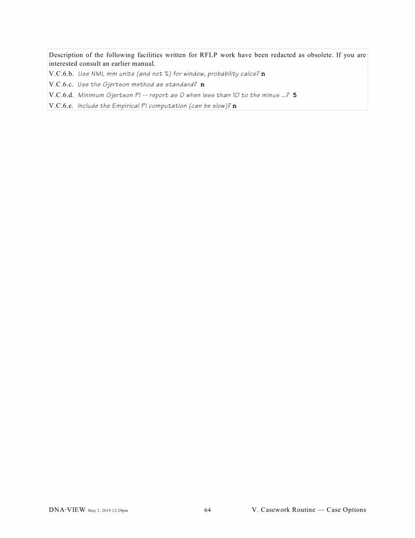
Description of the following facilities written for RFLP work have been redacted as obsolete. If you are
interested consult an earlier manual.
V.C.6.b. Use NML mm units (and not %) for window, probability calcs? n
V.C.6.c. Use the Gjertson method as standard? n
V.C.6.d. Minimum Gjertson PI -- report as 0 when less than 10 to the minus ...? 5
V.C.6.e. Include the Empirical PI computation (can be slow)? n
DNA@VIEW May 1, 2019 12:29pm V. Casework Routine — Case Options64
V.D. Automatic mixture and Manual mixed stain
V.D.1. Purpose
DNA·VIEW offers various methods for mixture computations – the “likelihood ratio” methods which are2
discussed in this section, and “exclusion” (implemented by DNA Exclusion , §V.I.).
V.D.2. Overview
V.D.2.a. Likelihood ratio mixture programs
The capabilities of the likelihood ratio programs include analysis of mixed stains, multiple contributors, and
victim contributions. The Mixture ("LR") calculator implements the likelihood ratio methods
V.D.2.a.i.) (binary) as discussed by Weir et al (1997). The result is given both numerically and
symbolically as an algebraic expression. The mixture ("LR") calculator is designed for maximum ease
of use and complete flexibility. It is available both
» (manual version) – as a top-level command (Casework < Manual mixed stain) which operates
simply as a high-powered spreadsheet calculator into which the user must type the alleles
(although scenarios may be saved and later retrieved and reworked),
» (automatic version) – and also as a sub-command of Automatic mixture (Casework <
Automatic mixture < select case, then mixture ("LR") calculator). This version begins with
imported (e.g. Import/Export < Genotyper import) case profile data including stain mixture and
references. The user designates which individual or combination of individuals (roles) is to be
regarded as stain, as suspect, and as (optional) victim.
Both versions allow modifying, adding, or deleting data in spreadsheet fashion, and saving your
work to retrieve and resume at a later date.
V.D.2.a.ii.) (continuous) with analysis approach similar to Puch-Solis et al (2013) incorporating intensity
(i.e. rfu) information and awareness of dropout, stutter, and other artifacts. Like the automatic binary
version, it uses imported profiles and the user designates the roles. The analysis is then automatic.
V.D.2.b. Theory
The mixture analysis paradigm considers four types of contribution (per Weir et al, 1997):
1 Mixture (aka stain aka unknown) is the set of alleles to be explained – typically a DNA mixture from
a crime scene.
2 Suspect (reference profile) is a person whose contribution is disputed. According to the first
hypothesis (numerator, usually the prosecution) the suspect contributed to the stain; according to the
second hypothesis (denominator, i.e. defense), the suspect did not contribute.
3 Victim (reference profile) is alleles whose source is not disputed. Typically “victim” is a rape victim
whose types are included in the vaginal mixture. The types of an acknowledged boyfriend or, in some
cases, a convicted or presumed accomplice rapist, are logically also coded as “victim.”
4 Unknown contributors. In addition to the explicitly specified alleles, the analysis model allows that
each of the prosecution and defense may stipulate 0 or more additional unknown, untyped, and
unrelated contributors to the mixture.
so-called, but this standard term isn’t well chosen since in reality the exclusion method also in effect2
takes a likelihood ratio approach.
DNA@VIEW May 1, 2019 12:29pm V. Casework Routine — Automatic mixture65
V.D.2.c. Practice examples (added – 2014)
There are two examples in the dnaview\examples folder. The example illustrations in this chapter
are from the first example, case 128.
NPmix.txt Import as “GeneMapper” format. This big example has many mixtures, suspects,
references, and includes rfu information. It will be case 128.
Hoffmix.txt Import as “Genotyper” format. This is an old small example with no rfu information.
It will be case 10089.
V.D.2.d. Operation (see §V.D.3 for details) (rewritten – 2014)
Note – prompts and report wording can be (partly) in Spanish or German according to the setting per
Housekeeping < Options < Language (§V.B.15).
Invoke either the stand-alone Case < Manual mixed stain, or the automatic version (e.g. via Open Case).
(NOTE - restrict data )3
The binary Mixture ("LR") calculator operation involves three main screens:
V.D.2.d.i.) Select mixture components
The screen shown in Figure 19 allows the user to define a scenario in which the victim, unknown, and
suspect profiles in terms of the roles in the case.
Operation then continues with the other screens alternately and iteratively.
V.D.2.d.ii.) Scenario calculation screen
From the scenario calculation screen (?) the user may select a locus to analyze or do various other
operations such as view a calculation summary.
V.D.2.d.iii.) Mixture computation screen
The mixture computation screen is a worksheet that computes the likelihood ratio for a single locus. The
screen is initially populated with any available data for the locus which may be either data from the case
(in case of automatic use) and/or any data previously entered and saved for the locus. The user may
modify the data in various ways, update the calculation, and exit back to the scenario calculation screen
(§V.D.2.d.ii).
V.D.3. Mixture ("LR") calculator operational details
Import and Open Case 128.
V.D.3.a. Define a scenario: select mixture components(revised – 2014)
V.D.3.a.i.) Type Z in the first line as the mixture. Hit enter which activates the down arrow (since it’s
the highlit button).
V.D.3.a.ii.) Put C for the suspect and G for the reference. Note that the SCROLL button becomes visible
when the input area is more leftward, so the scrolling trick (§V.D.3.a.v) is revealed.
Exceptionally, restrict data (§V.B.26) first – useful if you want to selective use some loci but not others,3
or to use only one of repeated assays for the same individual and locus.
DNA@VIEW May 1, 2019 12:29pm V. Casework Routine — Automatic mixture66
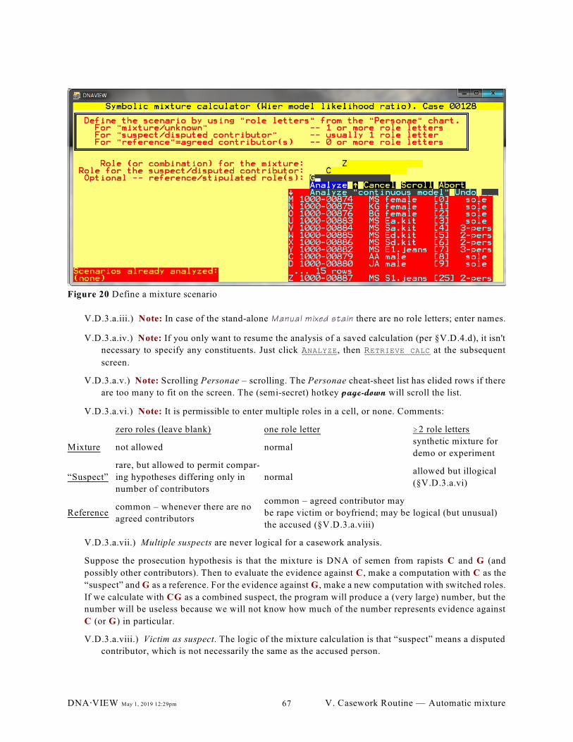
V.D.3.a.iii.) Note: In case of the stand-alone Manual mixed stain there are no role letters; enter names.
V.D.3.a.iv.) Note: If you only want to resume the analysis of a saved calculation (per §V.D.4.d), it isn't
necessary to specify any constituents. Just click ANALYZE, then RETRIEVE CALC at the subsequent
screen.
V.D.3.a.v.) Note: Scrolling Personae – scrolling. The Personae cheat-sheet list has elided rows if there
are too many to fit on the screen. The (semi-secret) hotkey page-down will scroll the list.
V.D.3.a.vi.) Note: It is permissible to enter multiple roles in a cell, or none. Comments:
zero roles (leave blank) one role letter $2 role letters
Mixture not allowed normalsynthetic mixture for
demo or experiment
“Suspect”
rare, but allowed to permit compar-
ing hypotheses differing only in
number of contributors
normalallowed but illogical
(§V.D.3.a.vi)
Referencecommon – whenever there are no
agreed contributors
common – agreed contributor may
be rape victim or boyfriend; may be
the accused (§V.D.3.a.viii)
logical (but unusual)
V.D.3.a.vii.) Multiple suspects are never logical for a casework analysis.
Suppose the prosecution hypothesis is that the mixture is DNA of semen from rapists C and G (and
possibly other contributors). Then to evaluate the evidence against C, make a computation with C as the
“suspect” and G as a reference. For the evidence against G , make a new computation with switched roles.
If we calculate with CG as a combined suspect, the program will produce a (very large) number, but the
number will be useless because we will not know how much of the number represents evidence against
C (or G) in particular.
V.D.3.a.viii.) Victim as suspect. The logic of the mixture calculation is that “suspect” means a disputed
contributor, which is not necessarily the same as the accused person.
Figure 20 Define a mixture scenario
DNA@VIEW May 1, 2019 12:29pm V. Casework Routine — Automatic mixture67
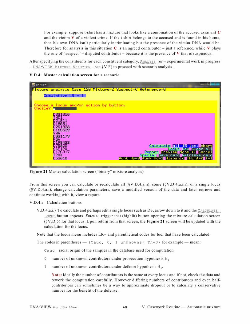
For example, suppose t-shirt has a mixture that looks like a combination of the accused assailant C
and the victim V of a violent crime. If the t-shirt belongs to the accused and is found in his home,
then his own DNA isn’t particularly incriminating but the presence of the victim DNA would be.
Therefore for analysis in this situation C is an agreed contributor – just a reference, while V plays
the role of “suspect” – disputed contributor – because it is the presence of V that is suspicious.
After specifying the constituents for each constituent category, ANALYZE (or – experimental work in progress
– DNA@VIEW MIXTURE SOLUTION – see §V.F) to proceed with scenario analysis.
V.D.4. Master calculation screen for a scenario
From this screen you can calculate or recalculate all (§V.D.4.a.ii), some (§V.D.4.a.iii), or a single locus
(§V.D.4.a.i), change calculation parameters, save a modified version of the data and later retrieve and
continue working with it, view a report.
V.D.4.a. Calculation buttons
V.D.4.a.i.) To calculate and perhaps edit a single locus such as D3, arrow down to it and the CALCULATE:
LOCUS button appears. Enter to trigger that (highlit) button opening the mixture calculation screen
(§V.D.5) for that locus. Upon return from that screen, the Figure 21 screen will be updated with the
calculation for the locus.
Note that the locus menu includes LR= and parenthetical codes for loci that have been calculated.
The codes in parentheses — (Cauc; 0, 1 unknowns; Th=0) for example — mean:
Cauc racial origin of the samples in the database used for computation
p0 number of unknown contributors under prosecution hypothesis H
d1 number of unknown contributors under defense hypothesis H .
Note: Ideally the number of contributors is the same at every locus and if not, check the data and
rework the computation carefully. However differing numbers of contributors and even half-
contributors can sometimes be a way to approximate dropout or to calculate a conservative
number for the benefit of the defense.
Figure 21 Master calculation screen (“binary” mixture analysis)
DNA@VIEW May 1, 2019 12:29pm V. Casework Routine — Automatic mixture68
Th=0 shows whether and what è value the computation uses.
LOCUS: NEW allows selection of a new locus for which the user may type in alleles. This is necessary
when using the Manual mixed stain version.
V.D.4.a.ii.) CALCULATE: ALL 15 LOCI automatically calculates or recalculates all loci. This
computation should be considered as only preliminary; almost for sure it will be necessary to review
locus by locus such as
» to resolve issues of dropout and interpretation
» to review the automatic assumptions about the numbers of unknown individuals who also
contributed to the profile, under each of prosecution and defense hypotheses.
V.D.4.a.iii.) CALCULATE: 7 LOCI automatically calculates remaining uncalculated (or cleared) loci but
does not change calculations already done.
V.D.4.a.iv.) LOCUS: CLEAR CALC a selected locus to remove the calculation for the locus. LOCUS:
CLEAR ALL deletes calculations from all loci. Any manual adjustments to alleles or interpretation (§?)
are retained.
V.D.4.a.v.) LOCUS: REMOVE deletes a locus including all the alleles and calculations entirely from the
scenario. (new – 2011)
V.D.4.b. Parameter settings
V.D.4.b.i.) # UNK HP and # UNK HD set the default number of unknown untyped persons to assume in
the mixture for hypotheses of prosecution and defense respectively. The actual number will be larger
if the default is insufficient to explain the observed alleles, or can be smaller if the user overrides on
a per-locus basis.
V.D.4.b.ii.) The current computation race is indicated by a button e.g. HISPANIC. Click it to respecify
the computation race. Recomputation requires an additional step – either revisiting individual loci
or CALCULATE: ALL ...
V.D.4.b.iii.) THETA= allows setting the inbreeding/relatedness parameter è, 0#è<1, for mixture
calculation. If è=0 the program produces a è-insensitive formula. If è>0, a è-sensitive formula per
Curran et al is derived and used.
V.D.4.b.iv.) The calculation rules for an allele marked sTutter are toggled with the T=I or T=N button.
See §V.D.5.e.ii.
V.D.4.c. Reporting (improved – 2014)
» REPORT: PREVIEW shows the report for the scenario calculation which can be printed or saved as
a text file. The report includes a summary paragraph with the overall LR and a line per locus, as
well as a paragraph per locus which is similar to the calculations screen for that locus.
» REPORT: DONE>> when through analyzing the present scenario. It bring you to a screen from
which you can initiate a new analysis scenario, and view reports for all scenarios so far computed
either per scenario (like that per PREVIEW or all together.
Note: "DONE" means that it will not be possible to resume and modify the scenario analysis
(unless you saved it per §V.D.4.d).
V.D.4.d. Interrupting your analysis (improved – 2014)
DNA@VIEW May 1, 2019 12:29pm V. Casework Routine — Automatic mixture69

» SAVE CALC to save the calculation to a special file from which it is possible to later resume the
same analysis.
» RETRIEVE CALC to retrieve and resume an analysis from the special file. Caution: If you open
Automatic mixture, select case (some number), and then retrieve an analysis saved from a
different case number, there may be confusion.
To resume analysis at a later date, note §V.D.3.a.iv.
DNA@VIEW May 1, 2019 12:29pm V. Casework Routine — Automatic mixture70
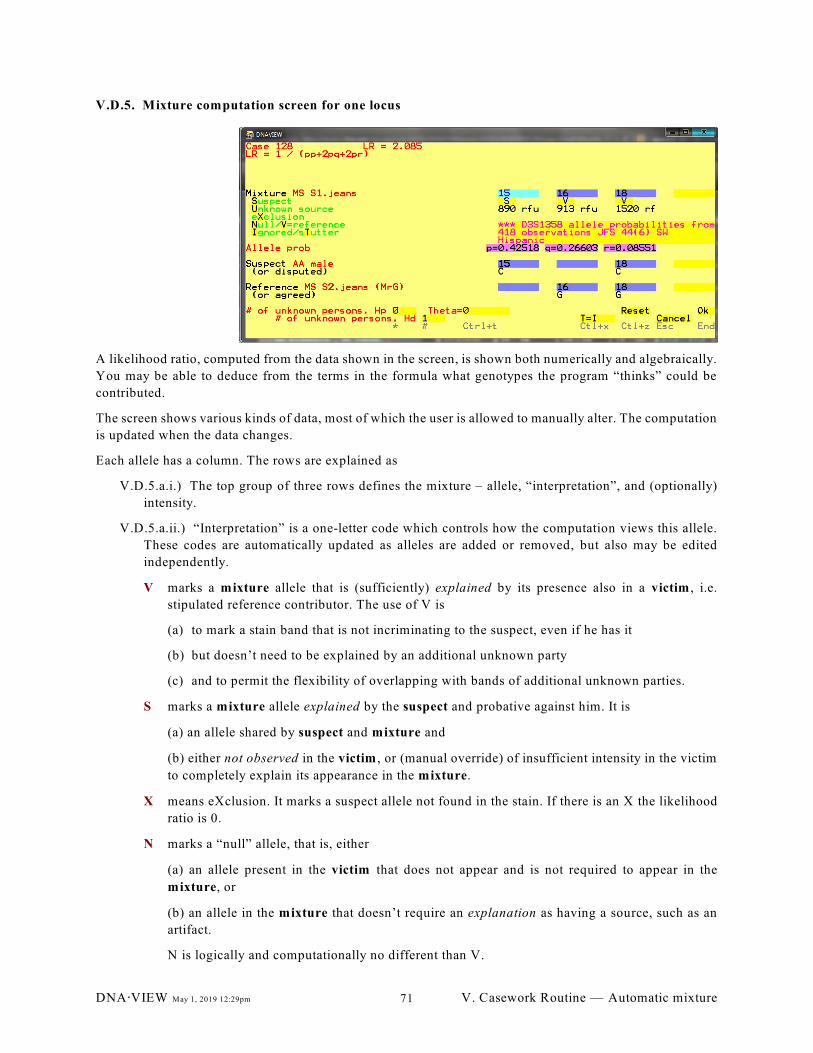
V.D.5. Mixture computation screen for one locus
A likelihood ratio, computed from the data shown in the screen, is shown both numerically and algebraically.
You may be able to deduce from the terms in the formula what genotypes the program “thinks” could be
contributed.
The screen shows various kinds of data, most of which the user is allowed to manually alter. The computation
is updated when the data changes.
Each allele has a column. The rows are explained as
V.D.5.a.i.) The top group of three rows defines the mixture – allele, “interpretation”, and (optionally)
intensity.
V.D.5.a.ii.) “Interpretation” is a one-letter code which controls how the computation views this allele.
These codes are automatically updated as alleles are added or removed, but also may be edited
independently.
V marks a mixture allele that is (sufficiently) explained by its presence also in a victim , i.e.
stipulated reference contributor. The use of V is
(a) to mark a stain band that is not incriminating to the suspect, even if he has it
(b) but doesn’t need to be explained by an additional unknown party
(c) and to permit the flexibility of overlapping with bands of additional unknown parties.
S marks a mixture allele explained by the suspect and probative against him. It is
(a) an allele shared by suspect and mixture and
(b) either not observed in the victim , or (manual override) of insufficient intensity in the victim
to completely explain its appearance in the mixture.
X means eXclusion. It marks a suspect allele not found in the stain. If there is an X the likelihood
ratio is 0.
N marks a “null” allele, that is, either
(a) an allele present in the victim that does not appear and is not required to appear in the
mixture, or
(b) an allele in the mixture that doesn’t require an explanation as having a source, such as an
artifact.
N is logically and computationally no different than V.
DNA@VIEW May 1, 2019 12:29pm V. Casework Routine — Automatic mixture71
U marks an allele in the mixture that is explained by neither victim nor suspect and hence must
be attributed to an unknown (and unrelated) person.
I means the column is ignored for computation, just as if it were deleted. (new – 2014)
T marks a probable stutter allele. See §V.D.5.e.ii. (new – 2014)
V.D.5.a.iii.) intensity. This information is optional and little used by the binary mixture program. It is
mainly displayed, if available, as a guide to the analyst. (new – 2014)
V.D.5.a.iv.) The allele probability used for computation. The exact value depends on the allele
probability Case Options (§V.C.4).
V.D.5.a.v.) “Suspect” alleles, or more precisely the reference type of a contributor assumed by the
prosecutor and disputed by the defense. Role letters under the alleles help visualization.
V.D.5.a.vi.) (optional) Reference alleles for any agreed contributors, such as a sexual assault victim.
Notes:
» (non-typical situation) When a mixture found in the suspect’s car includes the victim, probably
the roles of suspect and victim are reversed for purposed of calculation, the victim profile taking
the role of “suspect”, the suspect profile being an agreed reference.
» If the prosecution alleges an accomplice assailant, then the accomplice types should normally be
listed on the victim line, not suspect.
» If the mixture from a rape looks like a combination of suspect, victim, and the victim’s consensual
sexual partner, the victim and consual partner may both be considered as “victim”.
» In the case of a one-person “mixture” it is easier to use DNA Odds instead of Mixture ("LR")
calculator.
To remove an allele, use delete or replace it with 0.
If you enter an allele that exactly matches an existing allele in another row, the new allele will be moved
to the matching column if the slot is open.
The alleles can be entered in a variety of notations. In case of an STR system, the usual method of entry
is 9 or 9.3 or 9+3 or 10!1 indicating allele number and base pair offset. However 100 or more is
interpreted as base pairs, except that #123 again indicates allele number. RFLP alleles are interpreted as
base pairs, or as kilobases (e.g. 3.245) if less than 100.
V.D.5.b. Add an allele: Click in the box to the right of 18, and type 17 down-arrow.
V.D.5.b.i.) Automatic sorting – Note that the columns automatically sort and a new blank column for
allele 17 appears. (new – 2014)
V.D.5.b.ii.) Automatic LR recalculation: The LR calculation is updated. The # of unknowns for Hp had
to be incremented. (new – 2014)
V.D.5.c. Ignored allele. (new – 2014)
Type I down-arrow which marks allele 17 as ignored and positions entry in the space below.
V.D.5.c.i.) Automatic recalculation includes reducing # of unknowns Hp to the default value of 0, so the
LR is now the same as originally. Ignoring alleles is nicer than deleting them because it leaves them
documented.
V.D.5.d. Manual edit of rfu value (new – 2014)
DNA@VIEW May 1, 2019 12:29pm V. Casework Routine — Automatic mixture72
Type 140 up-arrow.
V.D.5.e. Stutter allele (new – 2014)
Type T enter which marks allele 17 as stutter. Two effects:
V.D.5.e.i.) Stutter allele heights are shown as % of the parent allele – in this case 9% of the +4 parent
18 – rather than rfu. (new – 2014)
V.D.5.e.ii.) For calculation, depending on user toggle button choice, stutter alleles are either
» treated as null (N – same as V=”no explanation needed”) if the toggle is T=N. The computation
then allows for the possibility that the allele might be a combination of stutter and an actual
(scant) contributor.
This treatment is usually conservative, i.e. more favorable to the accused and it is therefore the
default treatment. But it is easy to compare both calculations by toggling the T=... button to
be sure.
» ignored (I) if the toggle is T=I.
This option is sound if you are confident that no real signal is masked by the stutter. Also if
exceptionally this is the more conservative choice you might choose it for that reason.
Note Automatic stutter marking: By default the program will automatically mark T if the parent
allele is observed and the rfu ratio is no more than 2×stutter ratio for the locus. (Delete the
interpretation letter to allow the program to provide the default choice.)
V.D.5.f. Role letters
Below each suspect or reference allele is a role letter, such as C below the suspect 18 allele. This
documents where the allele comes from. Multiple letters are possible, either for homozygous
contributions or because of overlapping contributions when there are two references (or, unusually and
probably inadvisedly, two suspects ).4
V.D.5.f.i.) Considering the letters in combination with the rfu values can help the user to evaluate
whether Hp (especially) is plausible.5 (new – 2014)
V.D.5.f.ii.) Computation with roles: If and only if è>0 the letters affect the LR computation.
V.D.5.f.iii.) You can type a role to add an allele: (new – 2014)
Click under the empty suspect cell in the allele 16 column, i.e. in the role row and in between the two Cs.
Type the letter m up-arrow. Note that
» M appears in the cell (role letter entry is case-independent).
» 16 appears in the cell above.
V.D.5.g. Moving an allele
With the entry point in the 16 cell just created, type 17 enter. Note that
» The allele along with its role tag M move to the 17 column.
Even when the prosecution alleges (Hp) that the mixture is criminal defendants Jones and Smith, the4
fairest calculation is always to assume for purposes of evidence against Jones that Smith is a reference, not
an additional suspect, and conversely for evaluating evidence against Jones.
Future development: automatic plausibility evaluation5
DNA@VIEW May 1, 2019 12:29pm V. Casework Routine — Automatic mixture73
» The 17 column is automatically un-marked stutter. That seems the probable logical and useful
behavior when a contributor is alleged for the column, but you can manually re-mark it as stutter
if you insist.6
V.D.5.h. Buttons and parameters
There are four buttons and three parameters at the bottom of the screen. Activate/change any one by
clicking on it, or typing the hotkey.
The parameters (# unknown persons Hp or Hd, and theta) and the T=... toggle button override just for
this locus the default specified from the master calculation screen. (new – 2014)
V.D.5.h.i.) Hotkey tips. Beneath each in light grey is the name of the hotkey, i.e. type * to pop-up the
dialogue to change the # of unknowns for Hp. (new – 2014)
V.D.5.h.ii.) RESET action button: Click on the RESET button and the screen reverts to its initial state.
V.D.5.h.iii.) CANCEL action exits the locus computation screen back to the master computation screen
with no computation, result, or change.
V.D.5.h.iv.) OK button: Click this button – or end or ctrl-enter – to exit back to the master computation
screen with the computation for this locus.
V.D.6. Hints and techniques
If you understand how the mixture calculator works and use it expertly, then it has considerable flexibility
to cater to dropout, ambiguous stutter, and peak intensity information.
V.D.6.a. How to handle stutter
See §V.D.5.e.ii.
V.D.6.b. Taking account of peak area/height information
The current version of Mixture ("LR") calculator assigns interpretation letter codes (V, U etc.) without
regard to peak height/area. Under some circumstances it can be right to override the calculator’s
assumptions. For example suppose the mixture screen for some locus is
LR = 11 = 1/(2pr + 2qr + r )2
victim 12 14
stain 12 14 15
interpretation V V S
suspect 14 15
Suppose (as suggested by the boldface) that the mixture 12 is much weaker than the 14 and 15. Then the
analyst may decide that the weak contribution from the victim does not explain the 14 allele in the stain.
The way to take account of the extra information is manually type S as the interpretation of the 14 allele
to override the automatic interpretation, then click calculate:
Actually, marking it N makes a lot of sense in this situation.6
DNA@VIEW May 1, 2019 12:29pm V. Casework Routine — Automatic mixture74
LR = 20 = 1/2qr
victim 12 14
stain 12 14 15
interpretation V S S
suspect 14 15
V.D.6.c. Choosing the # of unknowns
The numerator and denominator of the likelihood ratio are probabilities that “belong” to the prosecution
and defense respectively. Since the prosecution wants the likelihood ratio to be large and the defense
wants it to be small, each side wants to make its own probability as large as possible.
For the prosecution this means choosing the most likely number — normally the obvious number — for
# of unknown persons Hp, subject to the limitation that it must be a scenario that the prosecutor is
willing to allege. This normally requires at least that the number of additional contributors be the same
for each locus, although exceptionally it could be that different numbers are an appropriate way to cater
to allelic dropout.
For the defense scenario, # of unknown persons, Hd similar considerations apply.
V.D.6.c.i.) Half an unknown person
The # of unknown persons is not required to be an integer; half-integers such as 0.5 or 1.5 are also
permitted. The idea behind this experimental feature is a possible way to be helpful or at least fair to the
defense by assuming (probably only for Hd) that an allele dropped out. Suppose for example that there
are three unexplained alleles under Hd. The usual practice would be to assume 2 unknown contributors,
or perhaps also to test the effect of 3 unknown contributors and give the defense the benefit of the smaller
number. Taking this generosity one step further, test the effect of 1.5 unknown contributors. If that gives
the lowest LR it may be the right number to report.
V.D.7. Comments
V.D.7.a. Crime Roles
V.D.7.a.i.) Use the role letters as you wish
The role names table (Figure 154, page 311) suggests for example using the role letter S for a
suspect. This is not obligatory. The actual meaning of a role letter for calculation depends on where
the user enters the letter in the screen shown in Figure 19, so you may use any letter however you
wish . However, if you choose to use the letter S for the mixture for example, then it might be
confusing if the report includes the word "suspect" next to the S. Therefore toggle the Case Options
"Omit role descriptions" option (§V.C.5.a) to "yes".
V.D.7.b. Limitations
V.D.7.b.i.) Kinship
There is no provision to take account of possible relationship between suspect and unknown. It is
expected to be included in Mixture Solution in the future.
V.D.7.b.ii.) Different races
All alleles at a locus are calculated as coming from the same population.
DNA@VIEW May 1, 2019 12:29pm V. Casework Routine — Automatic mixture75
V.D.8. Forensic Calculation Logic
Here are some examples of the way various scenarios are calculated.
V.D.8.a. Victim logic
Victim information is indicated by bands coded V on the calculation worksheet. Suppose for example
there are 4 bands in the stain of which two match the victim and the remaining ones (the “unexplainable
bands”) match the suspect and are coded S.
Normally the bands matching the victim would be coded V. In that case the matching calculation assumes
that there is only one assailant:
matching LR = 1/(2pq).
Whereas if there were no victim, or if for whatever reason you feel that there should be an additional
assailant providing the extra bands, then assuming two assailants we compute
matching LR = 1/(12pq).
V.D.8.b. Two or one matching bands
If the suspect has two bands matching the two unexplained bands, then the obvious calculation results
in a matching LR of 1/2pq.
If the suspect has one band that matches an unexplained band then the calculation (questionably) ignores
any extra suspect band. E.g. when there is only the one unexplained band, the matching LR is given as
1/q.
V.D.8.c. Multiple assailants
If there are extra unexplained bands not matched by the suspect, code them U and the multiple assailant
calculation is performed. More generally, if (# unknowns under Hd)>1, the calculation will take multiple
assailants into account.
For example, if the unexplained bands are PQRS and the suspect is PQ, the logic and computation is as
follows:
Imagine that the stain is fixed evidence, type=PQRS, and that the suspect’s type, PQ, is the evidence to
be evaluated probabilistically. That means we define
X=Pr(guilty suspect is PQ).
There are 6 consistent assailant types — PQ, PR, PS, QR, QS, RS — and they are equally likely once
guilt and this stain are assumed, so X=1/6. Similarly, we define
Y=Pr(innocent suspect is PQ),
so Y=2pq. Consequently the matching LR, representing the strength of evidence against this suspect, is
matching LR = X/Y = 1/(12pq).
V.D.9. Mixture test suite
The mixture examples option in the (Crime) Case menu calculates the LR formulas for a set of mixture
examples. Both è-sensitive (per Curran et al, 1999; see §V.D.4.b.iii) and è-less formulas are given. This suite
can be used as part of testing and validation of the mixture LR calculations.
DNA@VIEW May 1, 2019 12:29pm V. Casework Routine — Automatic mixture76
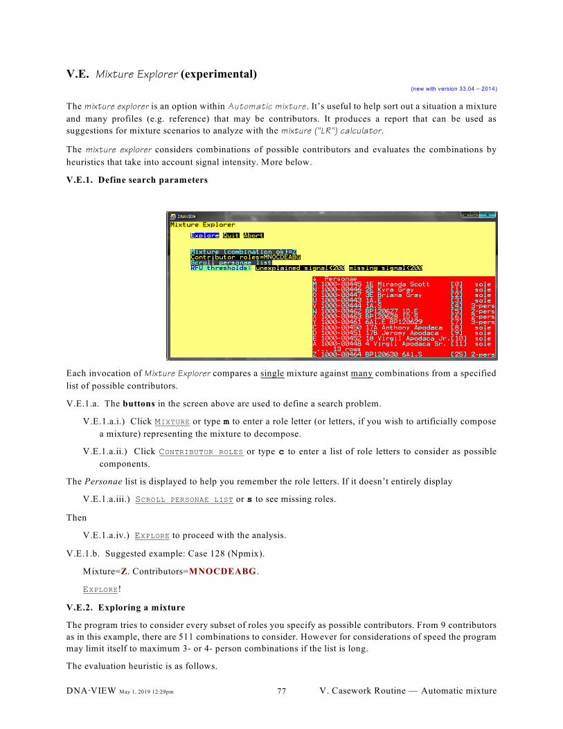
V.E. Mixture Explorer (experimental)(new with version 33.04 – 2014)
The mixture explorer is an option within Automatic mixture . It’s useful to help sort out a situation a mixture
and many profiles (e.g. reference) that may be contributors. It produces a report that can be used as
suggestions for mixture scenarios to analyze with the mixture ("LR") calculator.
The mixture explorer considers combinations of possible contributors and evaluates the combinations by
heuristics that take into account signal intensity. More below.
V.E.1. Define search parameters
Each invocation of Mixture Explorer compares a single mixture against many combinations from a specified
list of possible contributors.
V.E.1.a. The buttons in the screen above are used to define a search problem.
V.E.1.a.i.) Click MIXTURE or type m to enter a role letter (or letters, if you wish to artificially compose
a mixture) representing the mixture to decompose.
V.E.1.a.ii.) Click CONTRIBUTOR ROLES or type c to enter a list of role letters to consider as possible
components.
The Personae list is displayed to help you remember the role letters. If it doesn’t entirely display
V.E.1.a.iii.) SCROLL PERSONAE LIST or s to see missing roles.
Then
V.E.1.a.iv.) EXPLORE to proceed with the analysis.
V.E.1.b. Suggested example: Case 128 (Npmix).
Mixture=Z. Contributors=MNOCDEABG .
EXPLORE!
V.E.2. Exploring a mixture
The program tries to consider every subset of roles you specify as possible contributors. From 9 contributors
as in this example, there are 511 combinations to consider. However for considerations of speed the program
may limit itself to maximum 3- or 4- person combinations if the list is long.
The evaluation heuristic is as follows.
DNA@VIEW May 1, 2019 12:29pm V. Casework Routine — Automatic mixture77
V.E.2.a. For a given combination, the program guesses what proportion of each contributor best explains the
mixture. Thus, if nearly all of the alleles of some reference match high-rfu peaks in the mixture, a lot of
the mixture is explained by assuming that a large proportion of the mixture DNA (molecules or rfu) is
from that reference.
V.E.2.b. For the given combination and assumed proportions, another heuristic computes a degree-of-misfit
score (lower is better, 0=perfect fit), the “CHB” (that’s me) score.
V.E.3. Understanding the results
V.E.3.a. The combinations are sorted in order from lowest score to higher.
V.E.3.b. A report is produced showing the top several candidates. Following are a few examples with
explanations:
V.E.3.b.i.) The top suggestion, CHB score=270, asks Z ?=CG, meaning is Z=CG?
Z ?=CG; 1.6=misfit/locus if Z= 0.44xC 0.55xG All mixture alleles are explained by the references. All reference alleles are observed in the mixture.
About 44% of the mixture DNA rfu would come from C, 55% from D.
All the reported mixture alleles are alleles that exist in the C or G reference profiles.
All the alleles in the C or G reference profiles are reported in the mixture.
In short, the mixture has exactly the alleles you would expect if it is a mixture of C and G .
1.6=mixfit/locus is a score reflecting allelic height discrepancies between observed and expected
based on 44%C+55%D.
V.E.3.b.ii.) CAG explains the mixture nearly as well – not surprising if the A contribution is practically
0.
Z ?=CAG; 1.8=misfit/locus if Z= 0.44xC 0xA 0.55xG All mixture alleles are explained by the references. All reference alleles are observed in the mixture.
V.E.3.b.iii.) An example of a poor fit is EG with a bad (in context) score of 790.
Z ?=EG; 38=misfit/locus if Z= 0.084x? 0.3xE 0.61xG Max unexplained signal=710rfu. * =unexplained allele Max unobserved allele =660rfu. ()=unobserved but expected allele
D3S1358 15- 16- 17-(E 503) 18- D16S539 11- 12- 13-*708 D2S1338 22- 23- 24- 25-(E 367) CSF1PO 10-*625 11- 12- 14- TH01 6- 7- 9- 9.3-(E 663) VWA 14- 16- 17-(E 385) D21S11 29- 30-*223 32.2-(E 255) 33.2- TPOX 8- 10-(E 384) 11-
(I manually dug out the above analysis for demonstration. It would never appear on the report based on
the rfu thresholds above because there are discrepant alleles with rfu intensities above the specified
threshold of 200rfu.)
The heuristic best hypothesis includes a third unknown profile contributing 8.4% of the mixture.
Several E alleles are not observed in the mixture. These are noted in parentheses.
DNA@VIEW May 1, 2019 12:29pm V. Casework Routine — Automatic mixture78
» ()=unobserved allele. Based on a 30% contribution from E an allele #32.2 would be
expected at about 255rfu (E 255), but no such allele was observed.
Those alleles in the mixture but not explained by either E or G are indicated with an asterisk.
» *=unexplained allele. In D21 we see that the observed mixture alleles are 29, 30, 33.2.
The 30 allele was observed at 223rfu and – note the * – neither E nor G has that allele.
The loci listed are those at which either discrepancy occurs. The remaining loci that are not shown have
exactly the alleles of E+G .
DNA@VIEW May 1, 2019 12:29pm V. Casework Routine — Automatic mixture79
V.F. Mixture Solution – “continuous model” (experimental)(new with version 33.07 – 2014)
This program computes a mixture likelihood ratio using both allele size (i.e. repeat number) and intensity
(observed RFU). It thus is able to
» take into account artifacts and complications such as dropout and stutter;
» realize that two peaks of different heights, although they may be possible from one contributor
may be more likely from two contributors;
» estimate the proportional contributions from given references plus zero or more unknowns which
best explain the data;
» take into account the possibility of dropin (provisionally – a model for dropin is implemented but
I have not met anyone who seems confident that they know the right explanation for dropin);
The important consequence and benefit of all the above is that the program is able to
» make “sense” of complicated mixtures with 3 or 4, possibly even more, contributors;
» evaluate such mixtures objectively;
» produce a very high likelihood ratio against the suspect when justified;
» show why the suspect is not responsible when appropriate.
V.F.1. Expert system
Mixture analysis requires formulating and comparing analytically (that is, by computation) hypotheses for
prosecution and for defense. Mixture Solution, uniquely among mixture programs, automates that procedure.
Every other mixture program leaves to the expertise of the analyst to decide what hypotheses to evaluate,7
starting with specifying the number of contributors (per Clayton’s widely cited but impossible advice), and
also stating which reference profiles the prosecution and defense will assume are donors.
Mixture Solution offers a couple of alternatives:
V.F.1.a. Try all combinations
One alternative by Mixture Solution is that the program systematically tries all different combinations
and prefers the hypotheses that explain the mixture best. Fortunately the good speed of the program
makes this practical.
“All combinations” includes
V.F.1.a.i.) every subset combination of a list of reference profiles – i.e. from three people A B C, each
of the eight subsets ABC AB AC BC A B C and {} (none);
V.F.1.a.ii.) for each such subset, any number from zero up of additional “unknown” contributors;
V.F.1.a.iii.) compare every such hypothesis against every other, importantly including comparisons
between hypotheses with different numbers of contributors.
For example, see §xxx.
V.F.1.b. Wholesale evaluation of many donors
The “exclusion” method doesn’t require formulating hypotheses, but in part for that reason its results are7
meaningless hence we should not count implementations of the CPI, CPE, or RMNE method as “mixture
programs.”
DNA@VIEW May 1, 2019 12:29pm V. Casework Routine — Automatic mixture80
A useful heuristic trick to screen quickly a large number of potential donors or elimination samples. This
method is less rigorous than trying all combinations as §V.F.1.a but is even faster with a particularly large
set of donors to consider.
See §xxx
V.F.2. Caveat
A fair amount of validation work remains to be done. The program surely does reasonable things and provides
useful insight. Preliminary checking tells me that the model is robust in the sense that the results are not very
sensitive to parameter variations. However, it’s too soon to rely heavily on the results. And a future version
will surely include a provision to individualize the parameters for a particular lab’s work product.
One possible approach for casework is to make a preliminary and tentative continuous version analysis and
use it as an indication and a guide for a binary calculation.
The model permits user adjustment of the model parameters (§V.F.3.a.iii), but advice, especially automated
advice, on the values of those parameters is not well developed yet.
V.F.3. Operation of the continuous model
V.F.3.a. How to use
V.F.3.a.i.) Specify the role letters for mixture and possible reference profiles per §66.
V.F.3.a.ii.) Click DNA@VIEW MIXTURE SOLUTION.
V.F.3.a.iii.) Modify calculational parameters
Parameters affecting the calculation include maximum allowable number of unknown contributors,
rate of stochastic variation, detection threshold, modification to stutter, tolerance for dropin. The
initial, experimental release of the program does not allow the user to modify and experiment with
these values.
They are documented on the output.
V.F.3.a.iv.) Wait for computation to finish.
V.F.3.a.v.) Save and or print the report.
V.F.3.b. What the program does
V.F.3.b.i.) Decide how many unknown contributors
p dThe user has specified, under each of the competing hypotheses H and H , which reference profiles are
assumed to be contributors to the mixture. It is left to the program to decide how many additional
unknown and untyped contributors best explain the mixture. It does this by starting at zero and
incrementing (separately for each hypothesis). The searches continue until adding an additional
contributor makes things worse. “Worse” ideally means reducing the likelihood of the observed mixture.
But practically the search also has to stop when too many untyped contributors makes computation
unwieldly, as tends to happen with 3 or at most 4 such contributors.
V.F.3.b.ii.) Consider contributor proportions
Corresponding to each hypothesis, for any particular assumption as to the proportional contributions a
likelihood computation is rather quick. The program evaluates each hypotheses (of assumed references8
as slow as a second or two if there are three unknown contributors, for each of whom all the trillions of8
possible genotype combinations are considered; orders of magnitude quicker for fewer unknowns.
DNA@VIEW May 1, 2019 12:29pm V. Casework Routine — Automatic mixture81
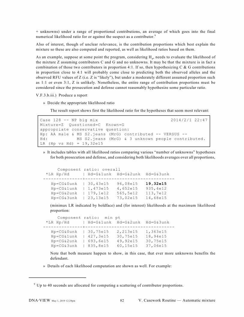
+ unknowns) under a range of proportional contributions, an average of which goes into the final
numerical likelihood ratio for or against the suspect as a contributor.9
Also of interest, though of unclear relevance, is the contribution proportions which best explain the
mixture so these are also computed and reported, as well as likelihood ratios based on them.
pAs an example, suppose at some point the program, considering H , needs to evaluate the likelihood of
the mixture Z assuming contributors C and G and no unknowns. It may be that the mixture is in fact a
combination of those two contributors in proportion 4:1. If so, then hypothesizing C & G contributions
in proportion close to 4:1 will probably come close to predicting both the observed alleles and the
observed RFU values of Z (i.e. Z is “likely”), but under a moderately different assumed proportion such
as 1:1 or even 3:1, Z is unlikely. Nonetheless, the entire range of contribution proportions must be
considered since the prosecution and defense cannot reasonably hypothesize some particular ratio.
V.F.3.b.iii.) Produce a report
» Decide the appropriate likelihood ratio
The result report shows first the likelihood ratio for the hypotheses that seem most relevant:
Case 128 -- NP big mix 2014/2/1 22:47Mixture=Z Questioned=C Known=Gappropriate conservative question:Hp: AA male & MS S2.jeans (MrG) contributed -- VERSUS --Hd: MS S2.jeans (MrG) & 3 unknown people contributed.LR (Hp vs Hd) = 19,32e15
» It includes tables with all likelihood ratios comparing various “number of unknowns” hypotheses
for both prosecution and defense, and considering both likelihoods averages over all proportions,
Component ratio: overall *LR Hp/Hd | Hd=G&1unk Hd=G&2unk Hd=G&3unk ---------------+---------------------------------- Hp=CG&0unk | 30,43e15 96,08e15 19,32e15 Hp=CG&1unk | 1,473e15 4,652e15 935,4e12 Hp=CG&2unk | 179,1e12 565,5e12 113,7e12 Hp=CG&3unk | 23,13e15 73,02e15 14,68e15
(minimax LR indicated by boldface) and (for interest) likelihoods at the maximum likelihood
proportion:
Component ratio: min pt *LR Hp/Hd | Hd=G&1unk Hd=G&2unk Hd=G&3unk ---------------+---------------------------------- Hp=CG&0unk | 30,75e15 2,213e15 1,363e15 Hp=CG&1unk | 427,3e15 30,75e15 18,94e15 Hp=CG&2unk | 693,6e15 49,92e15 30,75e15 Hp=CG&3unk | 835,8e15 60,15e15 37,06e15
Note that both measure happen to show, in this case, that ever more unknowns benefits the
defendant.
» Details of each likelihood computation are shown as well. For example:
Up to 40 seconds are allocated for computing a scattering of contributor proportions.9
DNA@VIEW May 1, 2019 12:29pm V. Casework Routine — Automatic mixture82
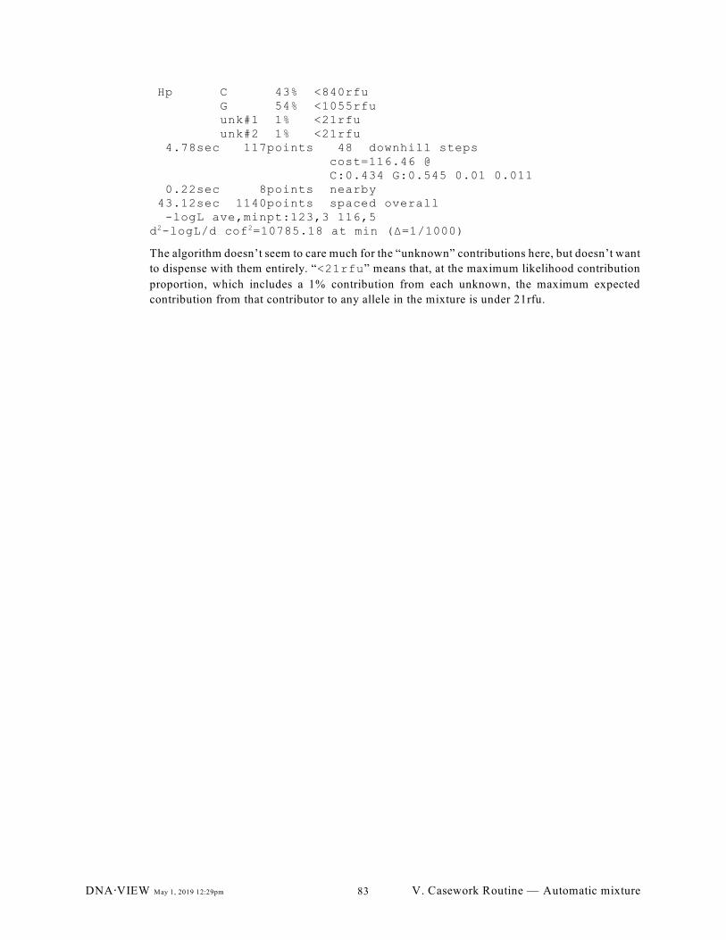
Hp C 43% <840rfu G 54% <1055rfu unk#1 1% <21rfu unk#2 1% <21rfu 4.78sec 117points 48 downhill steps cost=116.46 @ C:0.434 G:0.545 0.01 0.011 0.22sec 8points nearby 43.12sec 1140points spaced overall -logL ave,minpt:123,3 116,5d -logL/d cof =10785.18 at min (Ä=1/1000)2 2
The algorithm doesn’t seem to care much for the “unknown” contributions here, but doesn’t want
to dispense with them entirely. “<21rfu” means that, at the maximum likelihood contribution
proportion, which includes a 1% contribution from each unknown, the maximum expected
contribution from that contributor to any allele in the mixture is under 21rfu.
DNA@VIEW May 1, 2019 12:29pm V. Casework Routine — Automatic mixture83
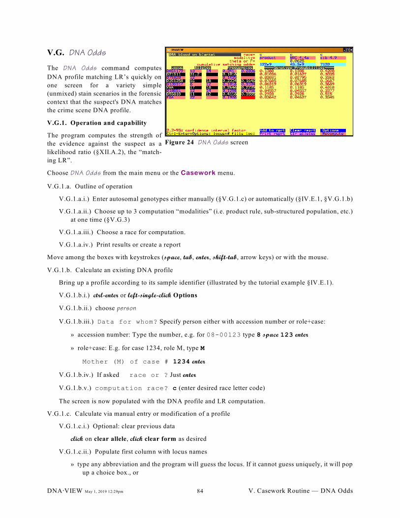
Figure 24 DNA Odds screen
V.G. DNA Odds
The DNA Odds command computes
DNA profile matching LR’s quickly on
one screen for a variety simple
(unmixed) stain scenarios in the forensic
context that the suspect's DNA matches
the crime scene DNA profile.
V.G.1. Operation and capability
The program computes the strength of
the evidence against the suspect as a
likelihood ratio (§XII.A.2), the “match-
ing LR”.
Choose DNA Odds from the main menu or the Casework menu.
V.G.1.a. Outline of operation
V.G.1.a.i.) Enter autosomal genotypes either manually (§V.G.1.c) or automatically (§IV.E.1, §V.G.1.b)
V.G.1.a.ii.) Choose up to 3 computation “modalities” (i.e. product rule, sub-structured population, etc.)
at one time (§V.G.3)
V.G.1.a.iii.) Choose a race for computation.
V.G.1.a.iv.) Print results or create a report
Move among the boxes with keystrokes (space, tab, enter, shift-tab, arrow keys) or with the mouse.
V.G.1.b. Calculate an existing DNA profile
Bring up a profile according to its sample identifier (illustrated by the tutorial example §IV.E.1).
V.G.1.b.i.) ctrl-enter or left-single-click Options
V.G.1.b.ii.) choose person
V.G.1.b.iii.) Data for whom? Specify person either with accession number or role+case:
» accession number: Type the number, e.g. for 08-00123 type 8 space 123 enter
» role+case: E.g. for case 1234, role M, type M
Mother (M) of case # 1234 enter
V.G.1.b.iv.) If asked race or ? Just enter
V.G.1.b.v.) computation race? c (enter desired race letter code)
The screen is now populated with the DNA profile and LR computation.
V.G.1.c. Calculate via manual entry or modification of a profile
V.G.1.c.i.) Optional: clear previous data
click on clear allele, click clear form as desired
V.G.1.c.ii.) Populate first column with locus names
» type any abbreviation and the program will guess the locus. If it cannot guess uniquely, it will pop
up a choice box., or
DNA@VIEW May 1, 2019 12:29pm V. Casework Routine — DNA Odds84
» type # for “next locus” according to the established locus order. Locus names will be filled in for
consecutive blank cells. Therefore:
» to completely populate the loci, clear the loci (§V.G.2.a.iv) then type # in the first locus position.
The loci and their order are defined per §IX.B.1.d.
V.G.1.c.iii.) Type in alleles as usual. (Only possible on a line that has a locus name entered.)
NOTE: If the allele resolution filter (ARF) is defined, then there will be a warning BEEP for any
allele not mentioned in the ARF.
V.G.1.c.iv.) Make a typical or demonstration profile
For amusement or demonstrations: Enter # for an allele and the program will substitute an allele
randomly selected based on the frequencies in` the relevant database.
Probabilities are calculated automatically, using the usual rules that are controlled by Case Options —
including Count this allele how many times? You may override the probability specification.
FEATURE: Small numbers — e.g. 0.0001 — are shown as 1/ — e.g. 1/1000. 1/23e6 means "1 in 23
million".
You may enter a number by entering its reciprocal — e.g. type in 100 to get 1/100. (But you cannot type
in the "e" notation.)
V.G.1.d. Choose alternate computation modalities(s)
V.G.1.d.i.) Move the type-in point (cursor) to any the three columns of the “modality” row, for example
with single-click.
V.G.1.d.ii.) Type all or part of the modality name if you know it. Or x space brings a pop-up menu of
modality choices (§V.G.3). Choose the desired one.
V.G.1.d.iii.) In the theta space below the modality, enter a theta value if relevant for that modality.
The "1/" convention also applies here. So for example if modality=relative and you want to consider
a 1/16 relative, just type 16 space.
V.G.1.e. Choose an alternate race
» click on any of the instances of the race letter at the top of the screen.
» Type in a new race letter.
You can choose any race; databases are chosen according to the established "defaults," or you
are prompted to select a database if there is no such. Present version uses the same race for all
three computations.
Your work & your locus list is saved across sessions.
V.G.2. Action keys and menus
V.G.2.a. Action keys. SINGLE(!)-left-click for the indicated action.
V.G.2.a.i.) Print reprt — immediately print a screen.
V.G.2.a.ii.) Add to rprt – add this screen to the report. (Print or save the report later with Print or with
File < save as.)
V.G.2.a.iii.) Clear reprt – Start the report afresh.
V.G.2.a.iv.) Clear alleles/form – Clear all the alleles, leaving the locus list, or clear everything.
DNA@VIEW May 1, 2019 12:29pm V. Casework Routine — DNA Odds85
After clicking clear alleles clears the alleles, the button name changes to clear form. Therefore, click
twice (slowly – these are single clicks) to clear everything.
V.G.2.a.v.) Options (also accessible via Ctrl-Enter) gives you a menu including the above choices and
also a few others:
» Person — prompts for an accession number, and collects the alleles for that person which is then
calculated as a profile.
This method can accept a profile with many loci. The extra loci, beyond a screenful, couldn’t be
typed directly into the DNA odds screen, but the larger profile can be created in DNAAVIEW
either through a method such as Genotyper Import, or Type in a Read (§IV.D.4).
» Append allele counts — include the allele count – database plus included observations – in the
printable report
» Uniqueness estimate — an experimental feature that illustrates how commonly the profile would
be seen in a random person who is not necessarily unrelated to the culprit.
V.G.3. “Modalities” of computation – various NRC II options
The matching LR is the likelihood ratio comparing the hypothesis
1H The suspect is the donor of the stain
against some other hypothesis.
V.G.3.a. product rule and variants
1These options compute the LR comparing H versus the alternative hypothesis
0H The suspect is unrelated to the donor.
Three calculation modes are available:
V.G.3.a.i.) product rule (i.e. theta=0)
V.G.3.a.ii.) NRC 4.4a (correction for homozygotes, your choice of theta)
V.G.3.a.iii.) both NRC 4.4a+b (correction for heterozygotes as well, your choice of theta)
V.G.3.b. relationship situations
When one of the relationship “modes” is specified, the calculation under “genotype frequency” (perhaps
misnamed) is f = Prob( DNA profile | donor = relative of suspect). The reported matching LR is 1/f
1(cumulated over all loci) and represents the likelihood ratio favoring H versus some "relative" alibi
2H The donor is a related to the suspect in a specified way.
V.G.3.b.i.) relative 4.8 (NRC II formula 4.8 with parameter F). By specifying an appropriate value for
4è (=F), any unilineal relationship can be specified. For example, è= / means the relative is a parent1
8or child and è= / means half-sibling, grandparent, uncle, niece, etc.1
V.G.3.b.ii.) sibling 4.9 (NRC II formula 4.9 for chance of similar sibling)
V.G.3.b.iii.) relative 4.10 (Balding & Nichols formula for when suspect & culprit are in the same sub-
population)
DNA@VIEW May 1, 2019 12:29pm V. Casework Routine — DNA Odds86
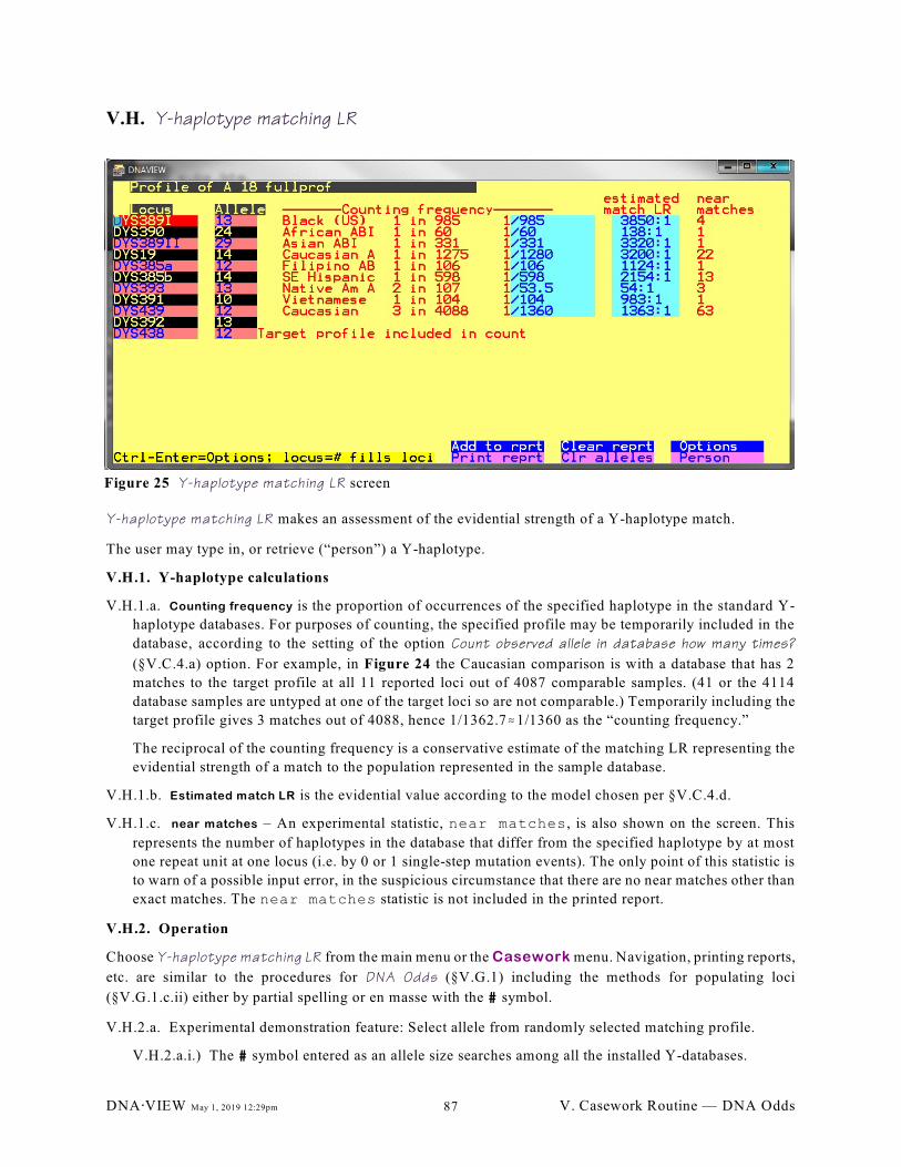
Figure 25 Y-haplotype matching LR screen
V.H. Y-haplotype matching LR
Y-haplotype matching LR makes an assessment of the evidential strength of a Y-haplotype match.
The user may type in, or retrieve (“person”) a Y-haplotype.
V.H.1. Y-haplotype calculations
V.H.1.a. Counting frequency is the proportion of occurrences of the specified haplotype in the standard Y-
haplotype databases. For purposes of counting, the specified profile may be temporarily included in the
database, according to the setting of the option Count observed allele in database how many times?
(§V.C.4.a) option. For example, in Figure 24 the Caucasian comparison is with a database that has 2
matches to the target profile at all 11 reported loci out of 4087 comparable samples. (41 or the 4114
database samples are untyped at one of the target loci so are not comparable.) Temporarily including the
target profile gives 3 matches out of 4088, hence 1/1362.7.1/1360 as the “counting frequency.”
The reciprocal of the counting frequency is a conservative estimate of the matching LR representing the
evidential strength of a match to the population represented in the sample database.
V.H.1.b. Estimated match LR is the evidential value according to the model chosen per §V.C.4.d.
V.H.1.c. near matches – An experimental statistic, near matches, is also shown on the screen. This
represents the number of haplotypes in the database that differ from the specified haplotype by at most
one repeat unit at one locus (i.e. by 0 or 1 single-step mutation events). The only point of this statistic is
to warn of a possible input error, in the suspicious circumstance that there are no near matches other than
exact matches. The near matches statistic is not included in the printed report.
V.H.2. Operation
Choose Y-haplotype matching LR from the main menu or the Casework menu. Navigation, printing reports,
etc. are similar to the procedures for DNA Odds (§V.G.1) including the methods for populating loci
(§V.G.1.c.ii) either by partial spelling or en masse with the # symbol.
V.H.2.a. Experimental demonstration feature: Select allele from randomly selected matching profile.
V.H.2.a.i.) The # symbol entered as an allele size searches among all the installed Y-databases.
DNA@VIEW May 1, 2019 12:29pm V. Casework Routine — DNA Odds87
V.H.2.a.ii.) A race letter (if accepted) as an allele selects a random matching profile from that race.
_______________________
See §VIII.F.2 for other Y-haplotype capabilities in DNA@VIEW including creating of Y-haplotype databases.
DNA@VIEW May 1, 2019 12:29pm V. Casework Routine — DNA Odds88
V.I. DNA Exclusion
The DNA Exclusion command computes the so-called “exclusion probability” for a DNA mixture quickly and
on one screen.
V.I.1. Discussion of the “exclusion” statistic
V.I.1.a. Definition
The “exclusion probability”, denoted A, is defined as the probability that a randomly selected person
would have an allele not detected in the specified crime stain profile (which is assumed to possibly be
a mixture), at any locus.
Examples:
V.I.1.a.i.) A suspect who is included in (or exactly matches) the crime stain profile for 10 loci, but has
an allele not in the profile at an 11 locus, is counted as excluded. th
NOTE: This may be an unrealistic assessment, for in practice perhaps it would be natural to re-
examine the crime stain, and to reinterpret the odd-ball locus as “inconclusive” if there is even a hint
of the “excluding” allele. If so, then actual “exclusion” decisions occur less often than the
“exclusion” computation says they do.
V.I.1.a.ii.) If the crime stain appears to be the result of a single contributor — having only one or two
alleles at each of many loci — and the crime stain is say 10,11 at some locus, the calculation counts
a potential homozygous 10 suspect as being not excluded. The exclusion formula takes no account
of the number of possible contributors.
V.I.1.a.iii.) If there is a non-zero null allele frequency (§VIII.C.12.e) specified for a particular locus, and
the crime stain is for example 10,11, then the calculation counts a potential 10,null or 11,null (or even
null,null) suspect as being not excluded.
The “probability of inclusion” or RMNE (proportion of “random men not excluded”) is 1!A.
V.I.1.b. Formula for “exclusion probability”
The exclusion probability, A, is computed as A=1!B, where B is the probability of inclusion (also referred
to as the RMNE). Note that B can be calculated locus-by-locus, vis: . The screen display
i(§V.I.2, Figure 26) shows the numbers B for each locus on the line for that locus, and the overall
numbers A and B at the top of the screen. For each locus i, the fraction of people eligible at that locus is
. For this purpose the probability Pr(G) of a genotype G is calculated as using the
product rule, conservatively modified by using the NRC II formula 4.4a for homozygous types:
Pr(QQ)=q +q(1!q)è.2
Genotypic combinations including the null allele are also counted. The null allele frequency is obtained
from the database. See §VIII.C.12.e.
Each allele probability is computed according to the rules detailed in §XIII.A.1.e covering minimum
allele frequency and “counting the observed allele.” Since each allele probability is computed separately
and independently, the resultant total probability may be slightly generous. If the total probability adds
to more than 1, a total of 1 is used instead. Note that the effect of the “generosity” is to understate slightly
the exclusion probability — normally a favor to the suspect.
V.I.1.c. Limitations of the “exclusion” method
V.I.1.c.i.) Ignores part of the evidence
DNA@VIEW May 1, 2019 12:29pm V. Casework Routine — DNA Exclusion89
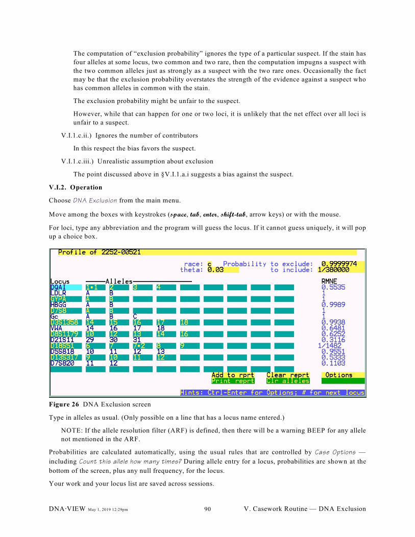
Figure 26 DNA Exclusion screen
The computation of “exclusion probability” ignores the type of a particular suspect. If the stain has
four alleles at some locus, two common and two rare, then the computation impugns a suspect with
the two common alleles just as strongly as a suspect with the two rare ones. Occasionally the fact
may be that the exclusion probability overstates the strength of the evidence against a suspect who
has common alleles in common with the stain.
The exclusion probability might be unfair to the suspect.
However, while that can happen for one or two loci, it is unlikely that the net effect over all loci is
unfair to a suspect.
V.I.1.c.ii.) Ignores the number of contributors
In this respect the bias favors the suspect.
V.I.1.c.iii.) Unrealistic assumption about exclusion
The point discussed above in §V.I.1.a.i suggests a bias against the suspect.
V.I.2. Operation
Choose DNA Exclusion from the main menu.
Move among the boxes with keystrokes (space, tab, enter, shift-tab, arrow keys) or with the mouse.
For loci, type any abbreviation and the program will guess the locus. If it cannot guess uniquely, it will pop
up a choice box.
Type in alleles as usual. (Only possible on a line that has a locus name entered.)
NOTE: If the allele resolution filter (ARF) is defined, then there will be a warning BEEP for any allele
not mentioned in the ARF.
Probabilities are calculated automatically, using the usual rules that are controlled by Case Options —
including Count this allele how many times? During allele entry for a locus, probabilities are shown at the
bottom of the screen, plus any null frequency, for the locus.
Your work and your locus list are saved across sessions.
DNA@VIEW May 1, 2019 12:29pm V. Casework Routine — DNA Exclusion90
V.I.2.a. Action keys
are the same as described in §V.G.2.a under DNA Odds.
V.I.2.b. Race
To compute with a different set of databases, click on the race letter and type a new race letter.
V.I.2.c. Theta
To compute with a different value of è, click on the theta box and type in a new value. Note that a
value larger than 1 will be inverted, so for example 0.01 may be entered by typing 100.
DNA@VIEW May 1, 2019 12:29pm V. Casework Routine — DNA Exclusion91
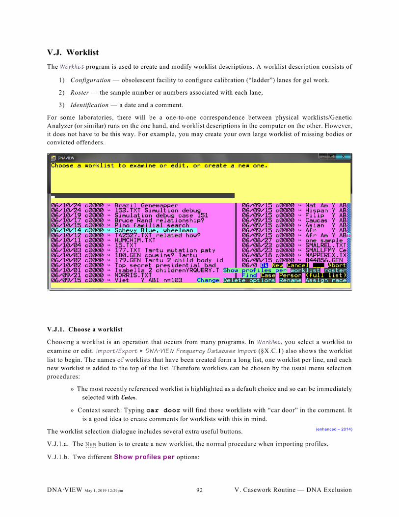
V.J. Worklist
The Worklist program is used to create and modify worklist descriptions. A worklist description consists of
1) Configuration — obsolescent facility to configure calibration (“ladder”) lanes for gel work.
2) Roster — the sample number or numbers associated with each lane,
3) Identification — a date and a comment.
For some laboratories, there will be a one-to-one correspondence between physical worklists/Genetic
Analyzer (or similar) runs on the one hand, and worklist descriptions in the computer on the other. However,
it does not have to be this way. For example, you may create your own large worklist of missing bodies or
convicted offenders.
V.J.1. Choose a worklist
Choosing a worklist is an operation that occurs from many programs. In Worklist, you select a worklist to
examine or edit. Import/Export < DNA@VIEW Frequency Database Import (§X.C.1) also shows the worklist
list to begin. The names of worklists that have been created form a long list, one worklist per line, and each
new worklist is added to the top of the list. Therefore worklists can be chosen by the usual menu selection
procedures:
» The most recently referenced worklist is highlighted as a default choice and so can be immediately
selected with Enter.
» Context search: Typing car door will find those worklists with “car door” in the comment. It
is a good idea to create comments for worklists with this in mind.
The worklist selection dialogue includes several extra useful buttons. (enhanced – 2014)
V.J.1.a. The NEW button is to create a new worklist, the normal procedure when importing profiles.
V.J.1.b. Two different Show profiles per options:
DNA@VIEW May 1, 2019 12:29pm V. Casework Routine — DNA Exclusion92
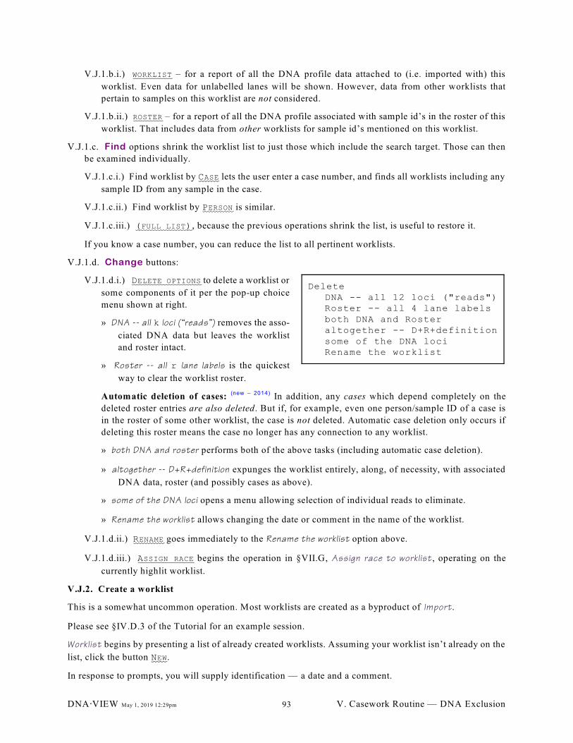
DeleteDNA -- all 12 loci ("reads")Roster -- all 4 lane labelsboth DNA and Rosteraltogether -- D+R+definitionsome of the DNA lociRename the worklist
V.J.1.b.i.) WORKLIST – for a report of all the DNA profile data attached to (i.e. imported with) this
worklist. Even data for unlabelled lanes will be shown. However, data from other worklists that
pertain to samples on this worklist are not considered.
V.J.1.b.ii.) ROSTER – for a report of all the DNA profile associated with sample id’s in the roster of this
worklist. That includes data from other worklists for sample id’s mentioned on this worklist.
V.J.1.c. Find options shrink the worklist list to just those which include the search target. Those can then
be examined individually.
V.J.1.c.i.) Find worklist by CASE lets the user enter a case number, and finds all worklists including any
sample ID from any sample in the case.
V.J.1.c.ii.) Find worklist by PERSON is similar.
V.J.1.c.iii.) (FULL LIST), because the previous operations shrink the list, is useful to restore it.
If you know a case number, you can reduce the list to all pertinent worklists.
V.J.1.d. Change buttons:
V.J.1.d.i.) DELETE OPTIONS to delete a worklist or
some components of it per the pop-up choice
menu shown at right.
» DNA -- all k loci (“reads”) removes the asso-
ciated DNA data but leaves the worklist
and roster intact.
» Roster -- all r lane labels is the quickest
way to clear the worklist roster.
Automatic deletion of cases: (new – 2014) In addition, any cases which depend completely on the
deleted roster entries are also deleted. But if, for example, even one person/sample ID of a case is
in the roster of some other worklist, the case is not deleted. Automatic case deletion only occurs if
deleting this roster means the case no longer has any connection to any worklist.
» both DNA and roster performs both of the above tasks (including automatic case deletion).
» altogether -- D+R+definition expunges the worklist entirely, along, of necessity, with associated
DNA data, roster (and possibly cases as above).
» some of the DNA loci opens a menu allowing selection of individual reads to eliminate.
» Rename the worklist allows changing the date or comment in the name of the worklist.
V.J.1.d.ii.) RENAME goes immediately to the Rename the worklist option above.
V.J.1.d.iii.) ASSIGN RACE begins the operation in §VII.G, Assign race to worklist , operating on the
currently highlit worklist.
V.J.2. Create a worklist
This is a somewhat uncommon operation. Most worklists are created as a byproduct of Import.
Please see §IV.D.3 of the Tutorial for an example session.
Worklist begins by presenting a list of already created worklists. Assuming your worklist isn’t already on the
list, click the button NEW.
In response to prompts, you will supply identification — a date and a comment.
DNA@VIEW May 1, 2019 12:29pm V. Casework Routine — DNA Exclusion93
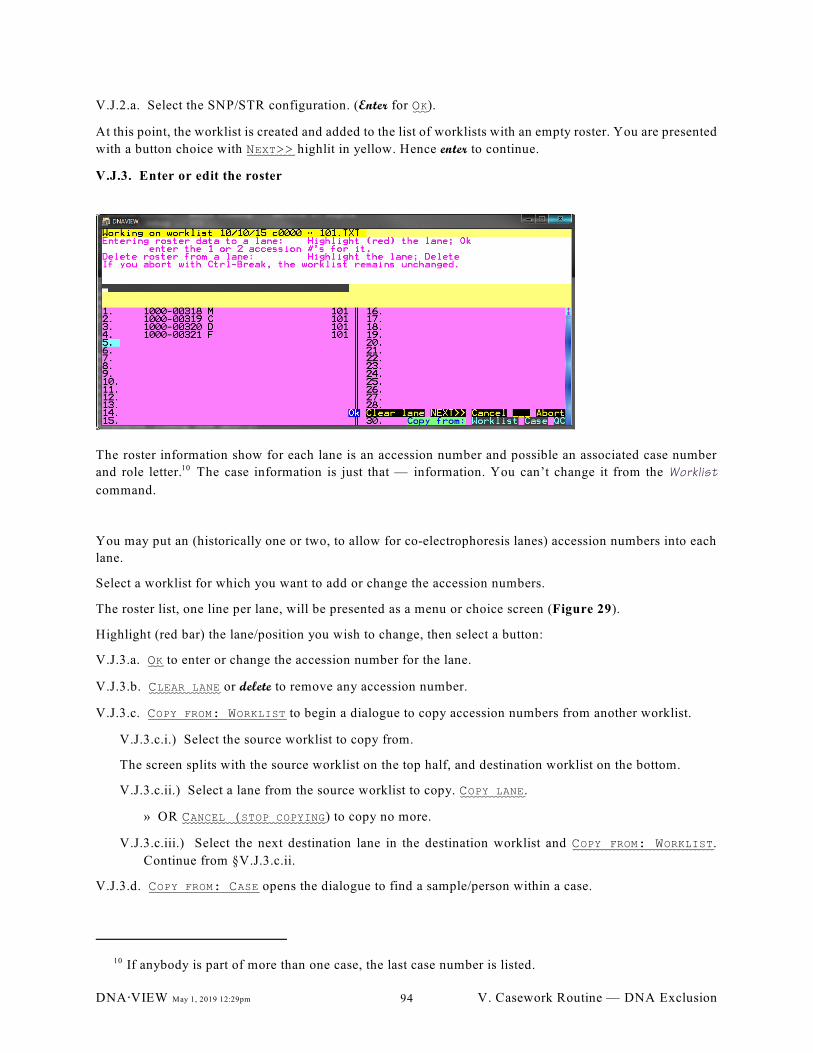
V.J.2.a. Select the SNP/STR configuration. (Enter for OK).
At this point, the worklist is created and added to the list of worklists with an empty roster. You are presented
with a button choice with NEXT>> highlit in yellow. Hence enter to continue.
V.J.3. Enter or edit the roster
The roster information show for each lane is an accession number and possible an associated case number
and role letter. The case information is just that — information. You can’t change it from the 10 Worklist
command.
You may put an (historically one or two, to allow for co-electrophoresis lanes) accession numbers into each
lane.
Select a worklist for which you want to add or change the accession numbers.
The roster list, one line per lane, will be presented as a menu or choice screen (Figure 29).
Highlight (red bar) the lane/position you wish to change, then select a button:
V.J.3.a. OK to enter or change the accession number for the lane.
V.J.3.b. CLEAR LANE or delete to remove any accession number.
V.J.3.c. COPY FROM: WORKLIST to begin a dialogue to copy accession numbers from another worklist.
V.J.3.c.i.) Select the source worklist to copy from.
The screen splits with the source worklist on the top half, and destination worklist on the bottom.
V.J.3.c.ii.) Select a lane from the source worklist to copy. COPY LANE.
» OR CANCEL (STOP COPYING) to copy no more.
V.J.3.c.iii.) Select the next destination lane in the destination worklist and COPY FROM: WORKLIST.
Continue from §V.J.3.c.ii.
V.J.3.d. COPY FROM: CASE opens the dialogue to find a sample/person within a case.
If anybody is part of more than one case, the last case number is listed.10
DNA@VIEW May 1, 2019 12:29pm V. Casework Routine — DNA Exclusion94
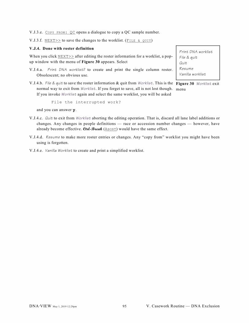
Print DNA worklist
File & quit
Quit
Resume
Vanilla worklist
Figure 30 Worklist exit
menu
V.J.3.e. COPY FROM: QC opens a dialogue to copy a QC sample number.
V.J.3.f. NEXT>> to save the changes to the worklist. (FILE & QUIT)
V.J.4. Done with roster definition
When you click NEXT>> after editing the roster information for a worklist, a pop-
up window with the menu of Figure 30 appears. Select
V.J.4.a. Print DNA worklist? to create and print the single column roster.
Obsolescent; no obvious use.
V.J.4.b. File & quit to save the roster information & quit from Worklist. This is the
normal way to exit from Worklist. If you forget to save, all is not lost though.
If you invoke Worklist again and select the same worklist, you will be asked
File the interrupted work?
and you can answer y.
V.J.4.c. Quit to exit from Worklist aborting the editing operation. That is, discard all lane label additions or
changes. Any changes in people definitions — race or accession number changes — however, have
already become effective. Ctrl-Break (ABORT) would have the same effect.
V.J.4.d. Resume to make more roster entries or changes. Any “copy from” worklist you might have been
using is forgotten.
V.J.4.e. Vanilla Worklist to create and print a simplified worklist.
DNA@VIEW May 1, 2019 12:29pm V. Casework Routine — DNA Exclusion95
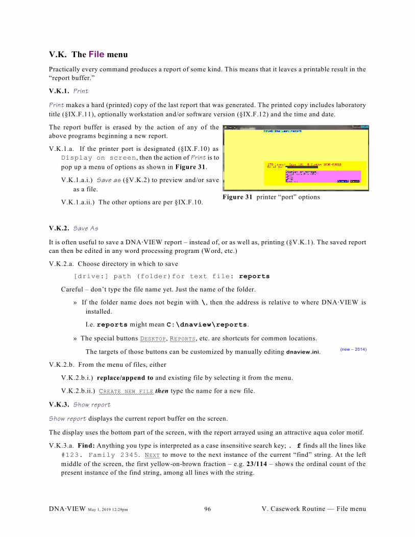
Figure 31 printer “port” options
V.K. The File menu
Practically every command produces a report of some kind. This means that it leaves a printable result in the
“report buffer.”
V.K.1. Print
Print makes a hard (printed) copy of the last report that was generated. The printed copy includes laboratory
title (§IX.F.11), optionally workstation and/or software version (§IX.F.12) and the time and date.
The report buffer is erased by the action of any of the
above programs beginning a new report.
V.K.1.a. If the printer port is designated (§IX.F.10) as
Display on screen, then the action of Print is to
pop up a menu of options as shown in Figure 31.
V.K.1.a.i.) Save as (§V.K.2) to preview and/or save
as a file.
V.K.1.a.ii.) The other options are per §IX.F.10.
V.K.2. Save As
It is often useful to save a DNA@VIEW report – instead of, or as well as, printing (§V.K.1). The saved report
can then be edited in any word processing program (Word, etc.)
V.K.2.a. Choose directory in which to save
[drive:] path (folder)for text file: reports
Careful – don’t type the file name yet. Just the name of the folder.
» If the folder name does not begin with \, then the address is relative to where DNA@VIEW is
installed.
I.e. reports might mean C:\dnaview\reports.
» The special buttons DESKTOP, REPORTS, etc. are shortcuts for common locations.
The targets of those buttons can be customized by manually editing dnaview.ini. (new – 2014)
V.K.2.b. From the menu of files, either
V.K.2.b.i.) replace/append to and existing file by selecting it from the menu.
V.K.2.b.ii.) CREATE NEW FILE then type the name for a new file.
V.K.3. Show report
Show report displays the current report buffer on the screen.
The display uses the bottom part of the screen, with the report arrayed using an attractive aqua color motif.
V.K.3.a. Find: Anything you type is interpreted as a case insensitive search key; . f finds all the lines like
#123. Family 2345. NEXT to move to the next instance of the current “find” string. At the left
middle of the screen, the first yellow-on-brown fraction – e.g. 23/114 – shows the ordinal count of the
present instance of the find string, among all lines with the string.
DNA@VIEW May 1, 2019 12:29pm V. Casework Routine — File menu96
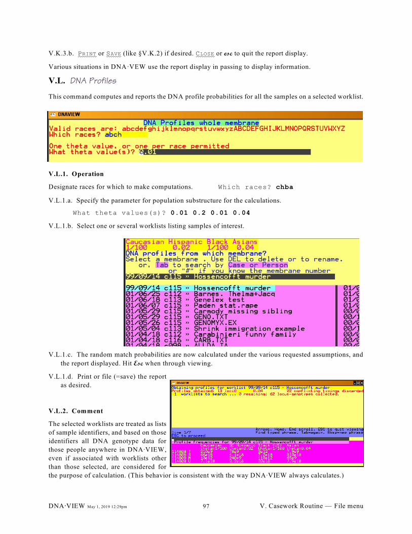
V.K.3.b. PRINT or SAVE (like §V.K.2) if desired. CLOSE or esc to quit the report display.
Various situations in DNA·VEW use the report display in passing to display information.
V.L. DNA Profiles
This command computes and reports the DNA profile probabilities for all the samples on a selected worklist.
V.L.1. Operation
Designate races for which to make computations. Which races? chba
V.L.1.a. Specify the parameter for population substructure for the calculations.
What theta values(s)? 0.01 0.2 0.01 0.04
V.L.1.b. Select one or several worklists listing samples of interest.
V.L.1.c. The random match probabilities are now calculated under the various requested assumptions, and
the report displayed. Hit Esc when through viewing.
V.L.1.d. Print or file (=save) the report
as desired.
V.L.2. Comment
The selected worklists are treated as lists
of sample identifiers, and based on those
identifiers all DNA genotype data for
those people anywhere in DNAAVIEW,
even if associated with worklists other
than those selected, are considered for
the purpose of calculation. (This behavior is consistent with the way DNAAVIEW always calculates.)
DNA@VIEW May 1, 2019 12:29pm V. Casework Routine — File menu97

DNA@VIEW May 1, 2019 12:29pm V. Casework Routine — File menu98
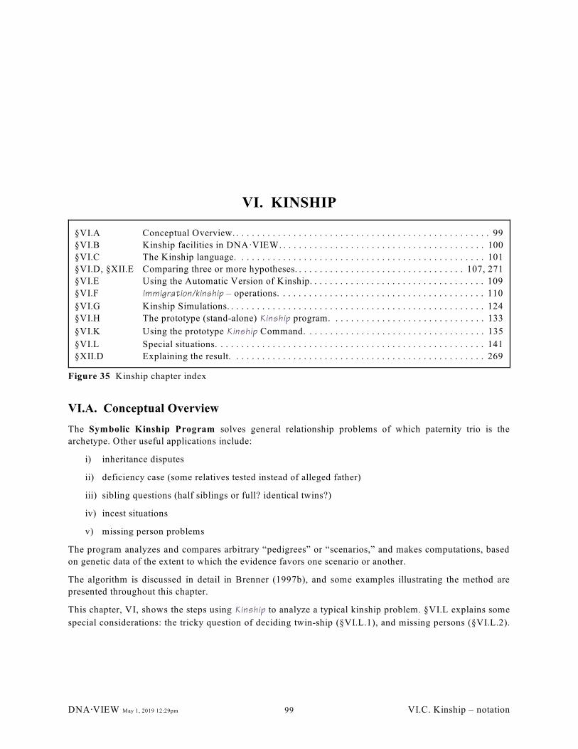
§VI.A Conceptual Overview. . . . . . . . . . . . . . . . . . . . . . . . . . . . . . . . . . . . . . . . . . . . . . . . . . 99
§VI.B Kinship facilities in DNA·VIEW. . . . . . . . . . . . . . . . . . . . . . . . . . . . . . . . . . . . . . . . 100
§VI.C The Kinship language. . . . . . . . . . . . . . . . . . . . . . . . . . . . . . . . . . . . . . . . . . . . . . . . 101
§VI.D, §XII.E Comparing three or more hypotheses. . . . . . . . . . . . . . . . . . . . . . . . . . . . . . . . . 107, 271
§VI.E Using the Automatic Version of Kinship. . . . . . . . . . . . . . . . . . . . . . . . . . . . . . . . . . 109
§VI.F Immigration/kinship – operations. . . . . . . . . . . . . . . . . . . . . . . . . . . . . . . . . . . . . . . . 110
§VI.G Kinship Simulations. . . . . . . . . . . . . . . . . . . . . . . . . . . . . . . . . . . . . . . . . . . . . . . . . . 124
§VI.H The prototype (stand-alone) Kinship program. . . . . . . . . . . . . . . . . . . . . . . . . . . . . . 133
§VI.K Using the prototype Kinship Command. . . . . . . . . . . . . . . . . . . . . . . . . . . . . . . . . . . 135
§VI.L Special situations. . . . . . . . . . . . . . . . . . . . . . . . . . . . . . . . . . . . . . . . . . . . . . . . . . . . 141
§XII.D Explaining the result. . . . . . . . . . . . . . . . . . . . . . . . . . . . . . . . . . . . . . . . . . . . . . . . . 269
Figure 35 Kinship chapter index
VI. KINSHIP
VI.A. Conceptual Overview
The Symbolic Kinship Program solves general relationship problems of which paternity trio is the
archetype. Other useful applications include:
i) inheritance disputes
ii) deficiency case (some relatives tested instead of alleged father)
iii) sibling questions (half siblings or full? identical twins?)
iv) incest situations
v) missing person problems
The program analyzes and compares arbitrary “pedigrees” or “scenarios,” and makes computations, based
on genetic data of the extent to which the evidence favors one scenario or another.
The algorithm is discussed in detail in Brenner (1997b), and some examples illustrating the method are
presented throughout this chapter.
This chapter, VI, shows the steps using Kinship to analyze a typical kinship problem. §VI.L explains some
special considerations: the tricky question of deciding twin-ship (§VI.L.1), and missing persons (§VI.L.2).
DNA@VIEW May 1, 2019 12:29pm VI.C. Kinship – notation99
VI.B. Kinship facilities in DNA·VIEW
VI.B.1. Two versions of Kinship
There are two versions of the Symbolic Kinship Program in DNA·VIEW – “immigration” and “Kinship.”
VI.B.1.a. immigration/kinship
The high-powered or “automatic” version of kinship (§VI.F, page 110) is a sub-command found in the
Automatic Kinship/Paternity/Automatic mixture (in Casework) menus. Hence, it is available in the
full DNA·VIEW system, but is not included in Abridged DNA·VIEW, in the DNA·VIEW Toolbox, or
in PATER.
It is an automated and greatly refined version of the prototype Kinship (§VI.B.1.b), which requires less
user attention and time, typically by one or two orders of magnitude, because it is integrated with the
population databases and the imported and stored profiles of DNAAVIEW. Therefore
VI.B.1.a.i.) A user interaction is not necessary for each locus separately.
VI.B.1.a.ii.) The program automatically determines the genotype patterns; you don’t type them in.
VI.B.1.a.iii.) The program automatically looks up the allele probabilities and calculates the likelihood
ratios.
VI.B.1.b. Kinship
is a command in the Research sub-menu. It is the original version, a prototype for the later one, and is
still essential in certain situations:
VI.B.1.b.i.) for the Kinship test suite (§VI.K.9);
VI.B.1.b.ii.) to obtain the formula for a hypothetical problem, without having any actual data;
VI.B.1.b.iii.) loci that are not defined as DNA loci;
VI.B.1.b.iv.) if you don’t have the full DNA·VIEW system, but only Abridged, Toolbox, or PATER.
VI.B.2. Limitations
The Kinship program (either version)
VI.B.2.a.i.) computes each locus independently and uses the product rule, so does not understand
haplotype systems such as Rh or HLA, and is at least theoretically inaccurate (magnitude of error not
clear) with X-linked markers, especially tightly linked ones, and with problems like sibship when any
two markers share a chromosome,
VI.B.2.a.ii.) assumes the same population group for all individuals;
VI.B.2.a.iii.) takes a simplified approach to mutations (§XIII.C.4).
Future development work may cater better to mutations.
DNA@VIEW May 1, 2019 12:29pm VI.C. Kinship – notation100
VI.C. The Kinship notation
Kinship cases are thus defined to the program using a fairly simple but general notation. Using this language
the user prepares a script and typically types it into the program using the Type in scenario option of the
automatic kinship version, or, in the case of the stand-alone Kinship program, Type in a new pedigree/locus.
VI.C.1. Kinship semantic concepts
The script defines normally two scenarios that are to be compared:11
VI.C.1.a. Principal scenario — The expected pedigree of a set of relationships among the people.
VI.C.1.b. Alternate scenario — An alternate pedigree or way they may be related.
It may include:
VI.C.1.c. Comments — these may describe the case, and perhaps (stand-alone Kinship only) make remarks
about a particular locus.
The script refers to various
VI.C.1.d. People — some typed, some may be untyped.
and, only in the case of the stand-along Kinship version:
VI.C.1.e. Phenotypes — for some or all of the people.
VI.C.2. Kinship syntax
Here are the basic syntax rules:
A kinship script consists of a collection of statements and/or comments.
Each statement either
(1) defines child-parent relationships,
(2) (stand-alone Kinship only) specifies genotypes for a person, or
(3) (stand-alone Kinship only) both.
VI.C.2.a. Names. The names of people must begin with a CAPITAL LETTER. Examples: Mom, C.
Note: The automatic version of kinship requires using a single letter name – namely the role letter –
for anyone for whom there is a DNA profile.
VI.C.2.b. Offspring-parent relationship. The three-place predicate with the punctuation marks : and +denotes the biological relationship among child, mother, and father. Example: C:Mom+F.
VI.C.2.c. Comment. Anything after a semicolon (;) on a line is a comment and is ignored by the program.
Example: C:Mom+F ; C is Charlie
VI.C.2.d. Alternatives. The symbol / designates the alternative scenario. It can be used in either of two
ways. The two methods below cannot be used together – use one or the other!
VI.C.2.d.i.) Simple but verbose way to designate alternatives
Put the / symbol in front of each line of the alternative scenario.
One hypothesis (§VI.C.4.b) or many hypothesis (§VI.D) are also possible.11
DNA@VIEW May 1, 2019 12:29pm VI.C. Kinship – notation101
VI.C.2.d.ii.) Concise but sometimes confusing way to designate alternatives
Let the / symbol separate two alternative names for the same role, one for each scenario.
Examples:
meaning: “Does the evidence support ...” Simple way Concise way
Paternity... paternity by F as opposed to by a guy
named Joe?
C : M + F
/ C : M + JoeC : M + F/Joe
missing
body (equi-
valent
ways)
... that the body C is the child of M and F,
as opposed to of some other parents?
C : M + F
/ C : Ma + FaC : M/Ma + F/Fa
... that the body C is the child of M and F,
as opposed to their child being someone
else?
C : M+F
/ Untyped:M+FC/Untyped : M+F
disaster
identif-
ication
... that C is the child and F the father, as
opposed to vice-versa?
C : M + F/ F : M + C
C/F : M + F/C
Advanced syntax rules (shortcuts):
VI.C.2.e. Statement separator
VI.C.2.e.i.) Multiple statements can be put on one line by separating them with the symbol % .
Example: C:M+F % D:M+F/YY ; C & D share mother M. Do they share father
F?
The same effect can always be obtained by using multiple lines and putting one statement per line.
VI.C.2.e.ii.) When using the “verbose” syntax method (/ at the beginning of alternative scenario lines),
there is just one / or string of / 's at the beginning of a line of several statements, not one / per
statement.
C:M+F % D:M+F ; primary hypothesis – full siblings
/ C:M+F % D:M+YY ; alternative hypothesis – half siblings
VI.C.2.e.iii.) More attractive alternative separators
symbol name method to type
Ë diamond Alt ~ (note: regardless of key caps, that's Alt with the upper-left-
most key)
' starburst Alt shift 8
1 cap Alt c
VI.C.2.f. Full siblings. As a shortcut, the comma (,) may be used to separate children who are full siblings.
Examples:
C, D : M + F/YY is equivalent to C:M+F/YY � D:M+F/YY.
C,E,D/Other : M+F is equivalent to
C:M+F � E:M+F � D/Other:M+F.
Notes: (1) There is no shortcut for half-sibling situations; a comma won’t help.
DNA@VIEW May 1, 2019 12:29pm VI.C. Kinship – notation102
(2) It’s better not to use the comma until you are fluent with the notation.
VI.C.2.g. Computer-generated names. For the lazy and unimaginative, the symbol ? can be used instead
of a name provided that
(i) The person is untyped.
(ii) The person is mentioned only once.
So for example H:?+Pa � J:?+Pa is exactly equivalent to H:Shirley+Pa � J:Belle+Pa
(assuming the mothers are untyped); both mean that H and J are half-siblings.
Note: It is better not to use this shortcut until you are fluent with the notation. For pitfalls, see §VII.F.2.
For a discussion, see §VI.C.4.a.
Examples using the shortcuts:
meaning: “Does the evidence support ...” Simple way Concise way
Paternity... paternity by F as opposed to by an un-
named person?
C : M + F/ C : M + ?
C : M + F/?
missing
body (equ-
ivalent
ways)
... that the body C is the child of M and F,
as opposed to of some other parents?
C : M + F
/ C : ? + ?C : M/? + F/?
... that the body C is the child of M and F,
as opposed to their child being someone
else?
C : M+F
/ ? : M+FC/? : M+F
avuncular... that F is the uncle of C, as opposed to
being unrelated?
C : M + Bro
Bro, F : ?+?/ C : M + ?
C : M + BroBro, F/? : ?+?
incest... that C’s father and uncle are the same
person? (“Mom” assumed to be untyped.)
C : Mom+U Mom, U : ?+?
/ ; empty line!
C : Mom+U/?
Mom, U : ?+?
sib-ship... that A and B are full siblings, as opposed
to being unrelated? (Parents not typed.)
A, B : ?+?
/ ; empty line!A, B/? : ?+?
VI.C.3. How to learn the Kinship Notation
The Kinship program computes a likelihood ratio comparing two different pedigrees as explanations for the
same genetic data.
VI.C.3.a. Two pictures
The first step in transcribing a kinship problem into DNA·VIEW is to draw two pedigrees, on the left and
right hand sides of the page, representing the two alternative explanations. Each pedigree is a diagram
consisting of one or more family trees.
DNA@VIEW May 1, 2019 12:29pm VI.C. Kinship – notation103
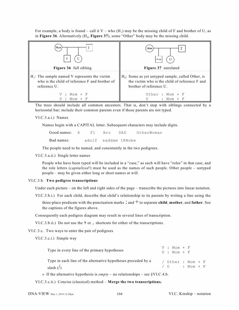
1For example, a body is found – call it V – who (H ) may be the missing child of F and brother of U, as
0in Figure 36. Alternatively (H , Figure 37), some “Other” body may be the missing child.
Figure 36 full sibling Figure 37 unrelated
1H : The sample named V represents the victim
who is the child of reference F and brother of
reference U.
0H : Some as yet untyped sample, called Other, is
the victim who is the child of reference F and
brother of reference U.
V : Mom + FU : Mom + F
Other : Mom + FU : Mom + F
The trees should include all common ancestors. That is, don’t stop with siblings connected by a
horizontal bar; include their common parents even if those parents are not typed.
VI.C.3.a.i.) Names
Names begin with a CAPITAL letter. Subsequent characters may include digits.
Good names: X F1 Bro DAD OtherWoman
Bad names: adolf saddam 1KNobe
The people need to be named, and consistently in the two pedigrees.
VI.C.3.a.ii.) Single letter names
People who have been typed will be included in a “case,” as such will have “roles” in that case, and
the role letters (capitalized!) must be used as the names of such people. Other people – untyped
people – may be given either long or short names at will.
VI.C.3.b. Two pedigree transcriptions
Under each picture – on the left and right sides of the page – transcribe the pictures into linear notation.
VI.C.3.b.i.) For each child, describe that child’s relationship to its parents by writing a line using the
three-place predicate with the punctuation marks : and + to separate child, mother, and father. See
the captions of the figures above.
Consequently each pedigree diagram may result in several lines of transcription.
VI.C.3.b.ii.) Do not use the ? or , shortcuts for either of the transcriptions.
VI.C.3.c. Two ways to enter the pair of pedigrees
VI.C.3.c.i.) Simple way
Type in every line of the primary hypothesesV : Mom + FU : Mom + F
Type in each line of the alternative hypotheses preceded by a
slash (/)
/ Other : Mom + F/ U : Mom + F
» If the alternative hypothesis is empty – no relationships – see §VI.C.4.b.
VI.C.3.c.ii.) Concise (classical) method – Merge the two transcriptions.
DNA@VIEW May 1, 2019 12:29pm VI.C. Kinship – notation104
In the middle of the page, merge the two transcriptions into a single set of statements by using the
symbol / wherever necessary to separate alternate versions of the same person. Thus:
V/Other : Mom + F U : Mom + F
To be rigorous about what is needed at this step: The program will take the merged description and
scan it twice, once reading only name on the left side of each /, and once reading only the name on
the right side of each /. These two scans must recover the two different transcriptions written in step
§VI.C.3.b.
This method gives a more concise formulation but sometimes merging seems tricky.
The (either) result of §VI.C.3.c.ii may be typed into the program.
VI.C.3.d. The advanced notational convenience options – the ? for a computer-generated name, the comma
(,) for full siblings – can be introduced after the merging but I emphatically recommend against using
them before gaining experience.
VI.C.3.e. Genotype syntax (stand-alone Kinship only)
The genotypes for one locus can be included in the kinship script in either of two ways:
VI.C.3.e.i.) as a separate statement (line) for any typed person; the name of the person, then the
genotype:
V pqMom qr
VI.C.3.e.ii.) interlineated in a relationship statement:
V pq/Other : Mom qr + FU : Mom + F
As permitted shortcut for the very economical-minded, the name can be omitted if the genotype is
present:
pq/Other : Mom qr + FU : Mom + F
Of course, if the person needs to be referenced twice, as Mom in the above example, you still need
to include the name.
Genotypes are designated by one or two lower case letters, such as pq. A few special rules:
VI.C.3.e.iii.) The letter o can only be used for a null allele.
VI.C.3.e.iv.) Homozygotes are normally written with just one letter, like q. Writing qq instead is
normally equivalent, but it does also mean that qo is not a possibility. If you write simply q, the
Kinship analysis depends on the setting of the silent allele toggle — see §VI.K.2.a).
VI.C.3.e.v.) For an X-linked system, male types should be written with a dash, i.e. r-.
VI.C.4. Kinship Semantics, clarification, and examples
VI.C.4.a. Understanding the ?
The ? does not mean “alternate father.” It merely denotes any untyped person whom you do not care to
take the trouble of naming. It may be and often is used to denote an alternative father, but the
“alternative” meaning is not part of the semantics of the ? but comes rather from the syntactic fact of
following a /.
DNA@VIEW May 1, 2019 12:29pm VI.C. Kinship – notation105
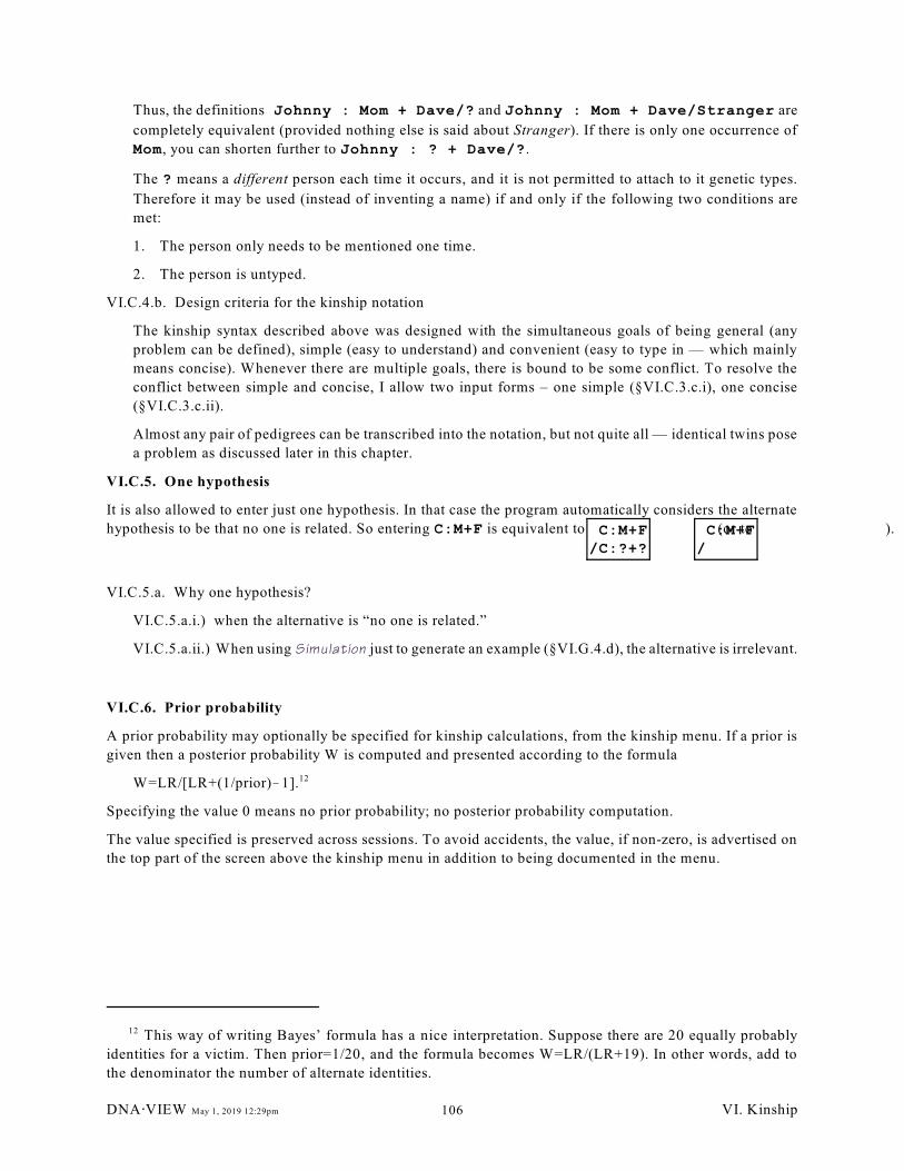
Thus, the definitions Johnny : Mom + Dave/? and Johnny : Mom + Dave/Stranger are
completely equivalent (provided nothing else is said about Stranger). If there is only one occurrence of
Mom, you can shorten further to Johnny : ? + Dave/?.
The ? means a different person each time it occurs, and it is not permitted to attach to it genetic types.
Therefore it may be used (instead of inventing a name) if and only if the following two conditions are
met:
1. The person only needs to be mentioned one time.
2. The person is untyped.
VI.C.4.b. Design criteria for the kinship notation
The kinship syntax described above was designed with the simultaneous goals of being general (any
problem can be defined), simple (easy to understand) and convenient (easy to type in — which mainly
means concise). Whenever there are multiple goals, there is bound to be some conflict. To resolve the
conflict between simple and concise, I allow two input forms – one simple (§VI.C.3.c.i), one concise
(§VI.C.3.c.ii).
Almost any pair of pedigrees can be transcribed into the notation, but not quite all — identical twins pose
a problem as discussed later in this chapter.
VI.C.5. One hypothesis
It is also allowed to enter just one hypothesis. In that case the program automatically considers the alternate
hypothesis to be that no one is related. So entering C:M+F is equivalent to (or to ). C:M+F/C:?+?
C:M+F/
VI.C.5.a. Why one hypothesis?
VI.C.5.a.i.) when the alternative is “no one is related.”
VI.C.5.a.ii.) When using Simulation just to generate an example (§VI.G.4.d), the alternative is irrelevant.
VI.C.6. Prior probability
A prior probability may optionally be specified for kinship calculations, from the kinship menu. If a prior is
given then a posterior probability W is computed and presented according to the formula
W=LR/[LR+(1/prior)!1].12
Specifying the value 0 means no prior probability; no posterior probability computation.
The value specified is preserved across sessions. To avoid accidents, the value, if non-zero, is advertised on
the top part of the screen above the kinship menu in addition to being documented in the menu.
This way of writing Bayes’ formula has a nice interpretation. Suppose there are 20 equally probably12
identities for a victim. Then prior=1/20, and the formula becomes W=LR/(LR+19). In other words, add to
the denominator the number of alternate identities.
DNA@VIEW May 1, 2019 12:29pm VI. Kinship106
VI.D. Multiple hypotheses in Kinship and Immigration/Kinship
A Kinship scenario may compare more than two hypotheses.
VI.D.1. Multiple hypothesis syntax
VI.D.1.a. example
The input syntax is based on the “simple method.” Example:
C:M+F ; Lines without leading / are the primary hypothesis.
/ C:M+Unc ; one leading / for the 1 alternate hypothesisst
/ Unc,F:?+?
// C:M+? ; two leading /’s for the 2 alternate, etc.nd
The three hypotheses are: The man F is the father; the man F is the uncle; the man F is unrelated.
VI.D.1.b. rules
VI.D.1.b.i.) Each line belongs to only one hypothesis. Thus any stipulated relationship – such as that M
is the mother of C in the example above – has to be stated repeatedly under each separate hypothesis.
VI.D.1.b.ii.) Each line begins (except for permitted leading spaces) with a string of 0 or more / 's,
indicating to which hypothesis the statement(s) of that line belong. If there are several statements on
a line (separated by statement separators §VI.C.2.e), all belong to the same hypothesis and the string
of / 's must be at the beginning of the line. If the statements for a hypothesis occupy more than one
line, each line must begin with the requisite number of / 's. Thus, the lines may be in any order.
VI.D.1.b.iii.) Any number of hypotheses are allowed. The primary hypothesis consists of the lines with
no / 's. A line with a string of n / 's is called the n alternative hypothesis.th
VI.D.2. Multiple hypothesis result
The result is a list of the relative likelihoods corresponding to the several hypotheses. For example:
400 : 100 : 1.
These correspond to the hypotheses primary, 1 alternative, 2 alternative.st nd
VI.D.2.a. Interpretation of multiple likelihoods
VI.D.2.a.i.) The ratio of any two likelihoods is the likelihood ratio supporting the first corresponding
hypothesis over the other one.
Thus, from the example above,
» 400 = 400:1 is the LR by which the evidence supports the primary hypothesis over the 2nd
alternate;
» 100 = 100:1 is the LR by which the evidence supports the 1 alternate hypothesis over the 2st nd
alternate;
» 4 = 400:100 is the LR by which the evidence supports the primary hypothesis over the 1 alternate.st
VI.D.2.a.ii.) “Overall” likelihood ratio
If the likelihood for the primary hypotheses is much greater than all the other likelihoods – if the
likelihood ratios are all greater than <threshold>, then we can conclude that the LR supporting the
primary hypothesis is at least <threshold>.
Example: 5@10 : 10 : 1 – primary hypothesis is supported by at least 5 million over either other9 3
hypothesis.
DNA@VIEW May 1, 2019 12:29pm VI. Kinship107
Example: 5@10 : 10 : 1 – primary hypothesis is not so strongly supported compared to an alternative.9 6
VI.D.2.b. Conclusions even when some LR's are less than <threshold>
If the primary hypothesis is not <threshold> better than all the other hypotheses we need to take a closer
look. Suppose the nearest rival is either
» not different in a significant way, or
» inherently not very plausible.
Then the data still may be good enough for a decision.
VI.D.2.c. Hypotheses give the same conclusion
The first case is the easier. Suppose that the hypotheses are
primary: remains V is Edward and remains W is Katie
1 alternative: V is Edward but W is unrelated to Katiest
2 alternative: V and W are unrelated to Edward and Katie,ne
that the likelihoods are 5@10 : 10 : 1, and that the threshold for identification is 10 . Then we can9 6 6
conclude that V=Edward because each of the first two explanations are at least <threshold> superior to
any explanation under which V�Edward.
VI.D.2.d. Dismissing inherently implausible explanations
“Inherently implausible” means having a particularly low prior probability. Therefore if we are willing
to assign prior probabilities to the various hypothesis we may be able to draw conclusions that go beyond
the simple-minded approach of §VI.D.2.a.ii.
VI.D.2.e. Posterior probabilities
The normal behavior of the prior probability parameter, that, if it is non-zero the program should compute
a posterior probability, does not apply in the case of multiple scenarios.
However, the Immigration/Kinship menu includes the experimental interactive option Bayes calculator
(§VI.F.6.e) to compute posterior probabilities as explained in §XII.E.1.f.
DNA@VIEW May 1, 2019 12:29pm VI. Kinship108
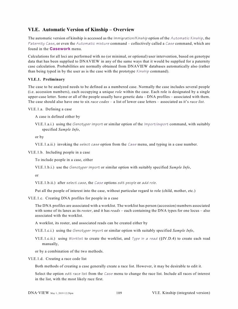
VI.E. Automatic Version of Kinship – Overview
The automatic version of kinship is accessed as the Immigration/Kinship option of the Automatic Kinship , the
Paternity Case, or even the Automatic mixture command – collectively called a Case command, which are
found in the Casework menu.
Calculations for all loci are performed with no (or minimal, or optional) user intervention, based on genotype
data that has been supplied to DNAVIEW in any of the same ways that it would be supplied for a paternity
case calculation. Probabilities are normally obtained from DNAVIEW databases automatically also (rather
than being typed in by the user as is the case with the prototype Kinship command).
VI.E.1. Preliminary
The case to be analyzed needs to be defined as a numbered case. Normally the case includes several people
(i.e. accession numbers), each occupying a unique role within the case. Each role is designated by a single
upper-case letter. Some or all of the people usually have genetic data – DNA profiles – associated with them.
The case should also have one to six race codes – a list of lower case letters – associated as it’s race list.
VI.E.1.a. Defining a case
A case is defined either by
VI.E.1.a.i.) using the Genotyper import or similar option of the Import/export command, with suitably
specified Sample Info,
or by
VI.E.1.a.ii.) invoking the select case option from the Case menu, and typing in a case number.
VI.E.1.b. Including people in a case
To include people in a case, either
VI.E.1.b.i.) use the Genotyper import or similar option with suitably specified Sample Info,
or
VI.E.1.b.ii.) after select case, the Case options edit people or add role.
Put all the people of interest into the case, without particular regard to role (child, mother, etc.)
VI.E.1.c. Creating DNA profiles for people in a case
The DNA profiles are associated with a worklist. The worklist has person (accession) numbers associated
with some of its lanes as its roster, and it has reads – each containing the DNA types for one locus – also
associated with the worklist.
A worklist, its roster, and associated reads can be created either by
VI.E.1.c.i.) using the Genotyper import or similar option with suitably specified Sample Info,
VI.E.1.c.ii.) using Worklist to create the worklist, and Type in a read (§IV.D.4) to create each read
manually,
or by a combination of the two methods.
VI.E.1.d. Creating a race code list
Both methods of creating a case generally create a race list. However, it may be desirable to edit it.
Select the option edit race list from the Case menu to change the race list. Include all races of interest
in the list, with the most likely race first.
DNA@VIEW May 1, 2019 12:29pm VI.E. Kinship (integrated version)109
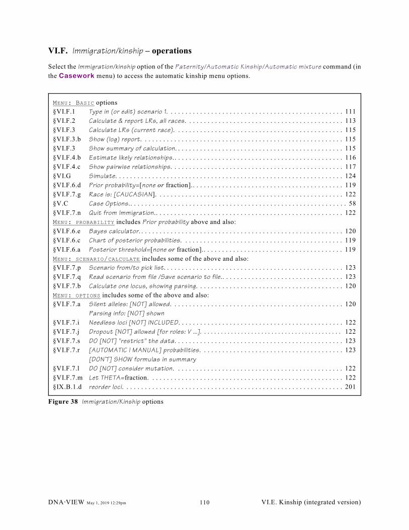
MENU: BASIC options
§VI.F.1 Type in (or edit) scenario 1. . . . . . . . . . . . . . . . . . . . . . . . . . . . . . . . . . . . . . . . . . . . . . . . 111
§VI.F.2 Calculate & report LRs, all races. . . . . . . . . . . . . . . . . . . . . . . . . . . . . . . . . . . . . . . . . . . 113
§VI.F.3 Calculate LRs (current race). . . . . . . . . . . . . . . . . . . . . . . . . . . . . . . . . . . . . . . . . . . . . . 115
§VI.F.3.b Show (log) report. . . . . . . . . . . . . . . . . . . . . . . . . . . . . . . . . . . . . . . . . . . . . . . . . . . . . . . 115
§VI.F.3 Show summary of calculation. . . . . . . . . . . . . . . . . . . . . . . . . . . . . . . . . . . . . . . . . . . . . . 115
§VI.F.4.b Estimate likely relationships.. . . . . . . . . . . . . . . . . . . . . . . . . . . . . . . . . . . . . . . . . . . . . . 116
§VI.F.4.c Show pairwise relationships. . . . . . . . . . . . . . . . . . . . . . . . . . . . . . . . . . . . . . . . . . . . . . . 117
§VI.G Simulate. . . . . . . . . . . . . . . . . . . . . . . . . . . . . . . . . . . . . . . . . . . . . . . . . . . . . . . . . . . . . . 124
§VI.F.6.d Prior probability=[none or fraction].. . . . . . . . . . . . . . . . . . . . . . . . . . . . . . . . . . . . . . . . . 119
§VI.F.7.g Race is: [CAUCASIAN]. . . . . . . . . . . . . . . . . . . . . . . . . . . . . . . . . . . . . . . . . . . . . . . . . . . 122
§V.C Case Options.. . . . . . . . . . . . . . . . . . . . . . . . . . . . . . . . . . . . . . . . . . . . . . . . . . . . . . . . . . . 58
§VI.F.7.n Quit from Immigration.. . . . . . . . . . . . . . . . . . . . . . . . . . . . . . . . . . . . . . . . . . . . . . . . . . . 122
MENU: PROBABILITY includes Prior probability above and also:
§VI.F.6.e Bayes calculator. . . . . . . . . . . . . . . . . . . . . . . . . . . . . . . . . . . . . . . . . . . . . . . . . . . . . . . . 120
§VI.F.6.c Chart of posterior probabilities. . . . . . . . . . . . . . . . . . . . . . . . . . . . . . . . . . . . . . . . . . . . 119
§VI.F.6.a Posterior threshold=[none or fraction].. . . . . . . . . . . . . . . . . . . . . . . . . . . . . . . . . . . . . . 119
MENU: SCENARIO/CALCULATE includes some of the above and also:
§VI.F.7.p Scenario from/to pick list. . . . . . . . . . . . . . . . . . . . . . . . . . . . . . . . . . . . . . . . . . . . . . . . . 123
§VI.F.7.q Read scenario from file /Save scenario to file.. . . . . . . . . . . . . . . . . . . . . . . . . . . . . . . . . 123
§VI.F.7.b Calculate one locus, showing parsing. . . . . . . . . . . . . . . . . . . . . . . . . . . . . . . . . . . . . . . . 120
MENU: OPTIONS includes some of the above and also:
§VI.F.7.a Silent alleles: [NOT] allowed. . . . . . . . . . . . . . . . . . . . . . . . . . . . . . . . . . . . . . . . . . . . . . . 120
Parsing info: [NOT] shown
§VI.F.7.i Needless loci [NOT] INCLUDED. . . . . . . . . . . . . . . . . . . . . . . . . . . . . . . . . . . . . . . . . . . . . 122
§VI.F.7.j Dropout [NOT] allowed [for roles: V ...]. . . . . . . . . . . . . . . . . . . . . . . . . . . . . . . . . . . . . . . . . . 122
§VI.F.7.s DO [NOT] "restrict" the data. . . . . . . . . . . . . . . . . . . . . . . . . . . . . . . . . . . . . . . . . . . . . . 123
§VI.F.7.r [AUTOMATIC | MANUAL] probabilities. . . . . . . . . . . . . . . . . . . . . . . . . . . . . . . . . . . . . . . 123
[DON’T] SHOW formulas in summary
§VI.F.7.l DO [NOT] consider mutation. . . . . . . . . . . . . . . . . . . . . . . . . . . . . . . . . . . . . . . . . . . . . . 122
§VI.F.7.m Let THETA=fraction. . . . . . . . . . . . . . . . . . . . . . . . . . . . . . . . . . . . . . . . . . . . . . . . . . . . . 122
§IX.B.1.d reorder loci. . . . . . . . . . . . . . . . . . . . . . . . . . . . . . . . . . . . . . . . . . . . . . . . . . . . . . . . . . . . 201
Figure 38 Immigration/Kinship options
VI.F. Immigration/kinship – operations
Select the Immigration/kinship option of the Paternity/Automatic Kinship/Automatic mixture command (in
the Casework menu) to access the automatic kinship menu options.
DNA@VIEW May 1, 2019 12:29pm VI.E. Kinship (integrated version)110
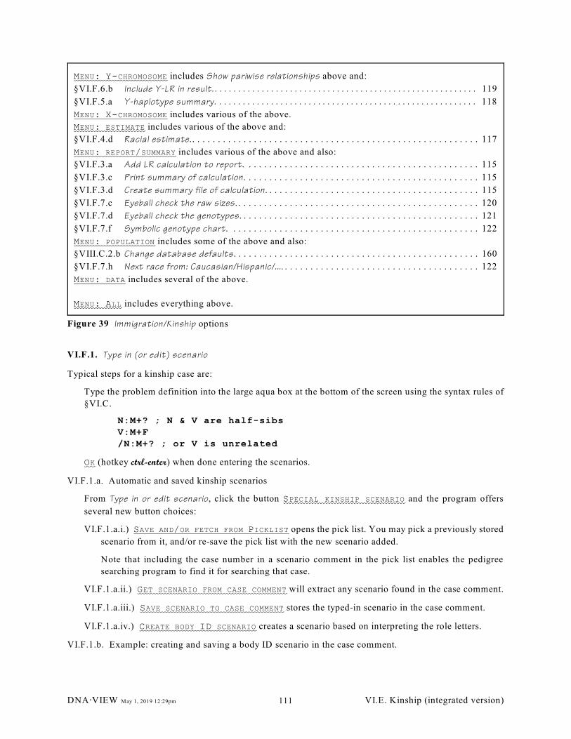
MENU: Y-CHROMOSOME includes Show pariwise relationships above and:
§VI.F.6.b Include Y-LR in result. . . . . . . . . . . . . . . . . . . . . . . . . . . . . . . . . . . . . . . . . . . . . . . . . . . . . . . . . 119
§VI.F.5.a Y-haplotype summary. . . . . . . . . . . . . . . . . . . . . . . . . . . . . . . . . . . . . . . . . . . . . . . . . . . . . . . . 118
MENU: X-CHROMOSOME includes various of the above.
MENU: ESTIMATE includes various of the above and:
§VI.F.4.d Racial estimate.. . . . . . . . . . . . . . . . . . . . . . . . . . . . . . . . . . . . . . . . . . . . . . . . . . . . . . . . 117
MENU: REPORT/SUMMARY includes various of the above and also:
§VI.F.3.a Add LR calculation to report. . . . . . . . . . . . . . . . . . . . . . . . . . . . . . . . . . . . . . . . . . . . . . 115
§VI.F.3.c Print summary of calculation. . . . . . . . . . . . . . . . . . . . . . . . . . . . . . . . . . . . . . . . . . . . . . 115
§VI.F.3.d Create summary file of calculation. . . . . . . . . . . . . . . . . . . . . . . . . . . . . . . . . . . . . . . . . . 115
§VI.F.7.c Eyeball check the raw sizes. . . . . . . . . . . . . . . . . . . . . . . . . . . . . . . . . . . . . . . . . . . . . . . . 120
§VI.F.7.d Eyeball check the genotypes. . . . . . . . . . . . . . . . . . . . . . . . . . . . . . . . . . . . . . . . . . . . . . . 121
§VI.F.7.f Symbolic genotype chart. . . . . . . . . . . . . . . . . . . . . . . . . . . . . . . . . . . . . . . . . . . . . . . . . 122
MENU: POPULATION includes some of the above and also:
§VIII.C.2.b Change database defaults. . . . . . . . . . . . . . . . . . . . . . . . . . . . . . . . . . . . . . . . . . . . . . . . 160
§VI.F.7.h Next race from: Caucasian/Hispanic/.... . . . . . . . . . . . . . . . . . . . . . . . . . . . . . . . . . . . . . . 122
MENU: DATA includes several of the above.
MENU: ALL includes everything above.
Figure 39 Immigration/Kinship options
VI.F.1. Type in (or edit) scenario
Typical steps for a kinship case are:
Type the problem definition into the large aqua box at the bottom of the screen using the syntax rules of
§VI.C.
N:M+? ; N & V are half-sibs
V:M+F/N:M+? ; or V is unrelated
OK (hotkey ctrl-enter) when done entering the scenarios.
VI.F.1.a. Automatic and saved kinship scenarios
From Type in or edit scenario, click the button SPECIAL KINSHIP SCENARIO and the program offers
several new button choices:
VI.F.1.a.i.) SAVE AND/OR FETCH FROM PICKLIST opens the pick list. You may pick a previously stored
scenario from it, and/or re-save the pick list with the new scenario added.
Note that including the case number in a scenario comment in the pick list enables the pedigree
searching program to find it for searching that case.
VI.F.1.a.ii.) GET SCENARIO FROM CASE COMMENT will extract any scenario found in the case comment.
VI.F.1.a.iii.) SAVE SCENARIO TO CASE COMMENT stores the typed-in scenario in the case comment.
VI.F.1.a.iv.) CREATE BODY ID SCENARIO creates a scenario based on interpreting the role letters.
VI.F.1.b. Example: creating and saving a body ID scenario in the case comment.
DNA@VIEW May 1, 2019 12:29pm VI.E. Kinship (integrated version)111
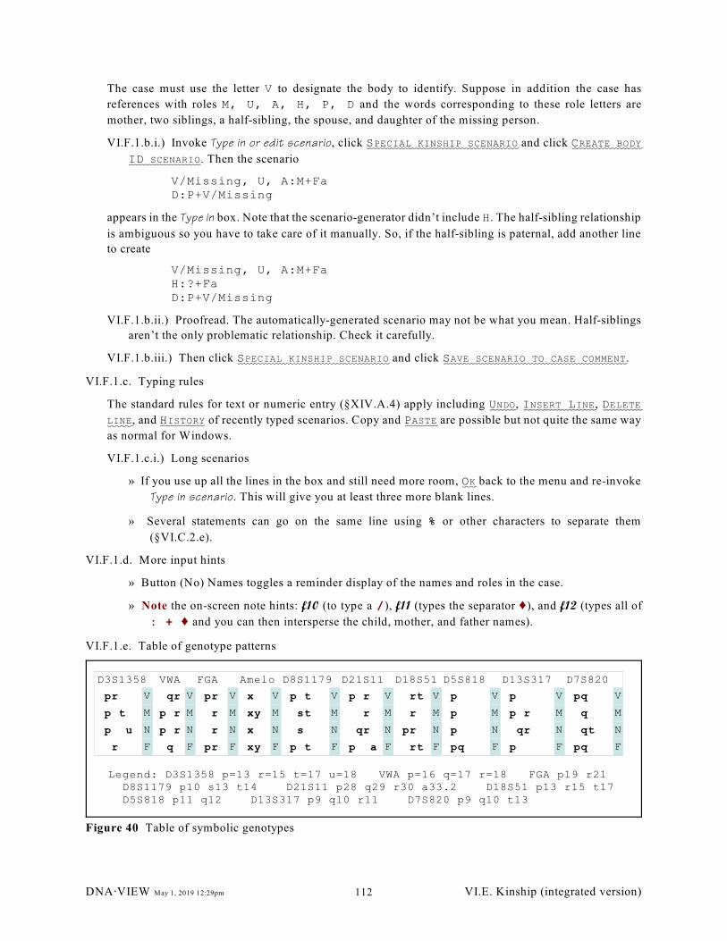
D3S1358 VWA FGA Amelo D8S1179 D21S11 D18S51 D5S818 D13S317 D7S820
pr V qr V pr V x V p t V p r V rt V p V p V pq V
p t M p r M r M xy M st M r M r M p M p r M q M
p u N p r N r N x N s N qr N pr N p N qr N qt N
r F q F pr F xy F p t F p a F rt F pq F p F pq F
Legend: D3S1358 p=13 r=15 t=17 u=18 VWA p=16 q=17 r=18 FGA p19 r21 D8S1179 p10 s13 t14 D21S11 p28 q29 r30 a33.2 D18S51 p13 r15 t17 D5S818 p11 q12 D13S317 p9 q10 r11 D7S820 p9 q10 t13
Figure 40 Table of symbolic genotypes
The case must use the letter V to designate the body to identify. Suppose in addition the case has
references with roles M, U, A, H, P, D and the words corresponding to these role letters are
mother, two siblings, a half-sibling, the spouse, and daughter of the missing person.
VI.F.1.b.i.) Invoke Type in or edit scenario, click SPECIAL KINSHIP SCENARIO and click CREATE BODY
ID SCENARIO. Then the scenario
V/Missing, U, A:M+FaD:P+V/Missing
appears in the Type in box. Note that the scenario-generator didn’t include H. The half-sibling relationship
is ambiguous so you have to take care of it manually. So, if the half-sibling is paternal, add another line
to create
V/Missing, U, A:M+FaH:?+FaD:P+V/Missing
VI.F.1.b.ii.) Proofread. The automatically-generated scenario may not be what you mean. Half-siblings
aren’t the only problematic relationship. Check it carefully.
VI.F.1.b.iii.) Then click SPECIAL KINSHIP SCENARIO and click SAVE SCENARIO TO CASE COMMENT.
VI.F.1.c. Typing rules
The standard rules for text or numeric entry (§XIV.A.4) apply including UNDO, INSERT LINE, DELETE
LINE, and HISTORY of recently typed scenarios. Copy and PASTE are possible but not quite the same way
as normal for Windows.
VI.F.1.c.i.) Long scenarios
» If you use up all the lines in the box and still need more room, OK back to the menu and re-invoke
Type in scenario. This will give you at least three more blank lines.
» Several statements can go on the same line using % or other characters to separate them
(§VI.C.2.e).
VI.F.1.d. More input hints
» Button (No) Names toggles a reminder display of the names and roles in the case.
» Note the on-screen note hints: f10 (to type a /), f11 (types the separator Ë), and f12 (types all of
: + Ë and you can then intersperse the child, mother, and father names).
VI.F.1.e. Table of genotype patterns
DNA@VIEW May 1, 2019 12:29pm VI.E. Kinship (integrated version)112
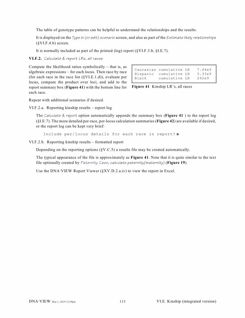
Caucasian cumulative LR 7.44e9Hispanic cumulative LR 5.33e9Black cumulative LR 292e9
Figure 41 Kinship LR’s, all races
The table of genotype patterns can be helpful to understand the relationships and the results.
It is displayed on the Type in (or edit) scenario screen, and also as part of the Estimate likely relationships
(§VI.F.4.b) screen.
It is normally included as part of the printed (log) report (§VI.F.3.b, §I.E.7).
VI.F.2. Calculate & report LRs, all races
Compute the likelihood ratios symbolically – that is, as
algebraic expressions – for each locus. Then race by race
(for each race in the race list (§VI.E.1.d)), evaluate per
locus, compute the product over loci, and add to the
report summary box (Figure 41) with the bottom line for
each race.
Repeat with additional scenarios if desired.
VI.F.2.a. Reporting kinship results – report log
The Calculate & report option automatically appends the summary box (Figure 41 ) to the report log
(§I.E.7). The more detailed per-race, per-locus calculation summaries (Figure 42) are available if desired,
or the report log can be kept very brief:
Include per/locus details for each race in report? n
VI.F.2.b. Reporting kinship results – formatted report
Depending on the reporting options (§V.C.5) a results file may be created automatically.
The typical appearance of the file is approximately as Figure 41. Note that it is quite similar to the text
file optionally created by Paternity Case, calculate paternity(maternity) (Figure 19).
Use the DNA@VIEW Report Viewer (§XV.D.2.a.iv) to view the report in Excel.
DNA@VIEW May 1, 2019 12:29pm VI.E. Kinship (integrated version)113
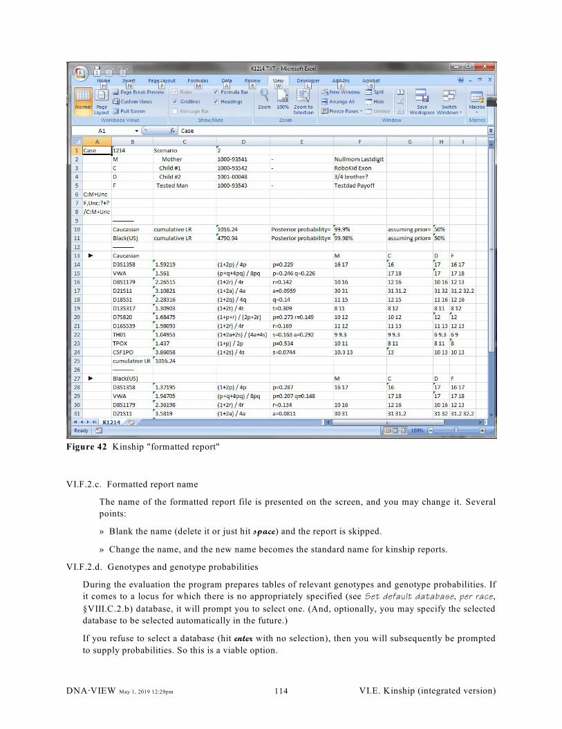
Figure 42 Kinship "formatted report"
VI.F.2.c. Formatted report name
The name of the formatted report file is presented on the screen, and you may change it. Several
points:
» Blank the name (delete it or just hit space) and the report is skipped.
» Change the name, and the new name becomes the standard name for kinship reports.
VI.F.2.d. Genotypes and genotype probabilities
During the evaluation the program prepares tables of relevant genotypes and genotype probabilities. If
it comes to a locus for which there is no appropriately specified (see Set default database, per race,
§VIII.C.2.b) database, it will prompt you to select one. (And, optionally, you may specify the selected
database to be selected automatically in the future.)
If you refuse to select a database (hit enter with no selection), then you will subsequently be prompted
to supply probabilities. So this is a viable option.
DNA@VIEW May 1, 2019 12:29pm VI.E. Kinship (integrated version)114
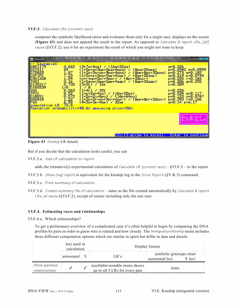
Figure 43 Kinship LR details
VI.F.3. Calculate LRs (current race)
computes the symbolic likelihood ratios and evaluates them only for a single race, displays on the screen
(Figure 43) and does not append the result to the report. As opposed to Calculate & report LRs, [all]
races (§VI.F.2), use it for an experiment the result of which you might not want to keep.
But if you decide that the calculation looks useful, you can
VI.F.3.a. Add LR calculation to report
adds the (tentatively) experimental calculation of Calculate LR (current race) – §VI.F.3 – to the report.
VI.F.3.b. Show (log) report is equivalent for the kinship log to the Show Report (§V.K.3) command.
VI.F.3.c. Print summary of calculation
VI.F.3.d. Create summary file of calculation – same as the file created automatically by Calculate & report
LRs, all races (§VI.F.2), except of course including only the one race.
VI.F.4. Estimating races and relationships
VI.F.4.a. Which relationships?
To get a preliminary overview of a complicated case it’s often helpful to begin by comparing the DNA
profiles by pairs in order to guess who is related and how closely. The immigration/kinship menu includes
three different computation options which are similar in spirit but differ in data and details.
loci used in
calculationDisplay format
autosomal Y LR’ssymbolic genotype chart
autosomal loci Y loci
Show pairwise
relationshipsT T
scrollable/sortable menu shows
up to all 5 LRs for every pairnone
DNA@VIEW May 1, 2019 12:29pm VI.E. Kinship (integrated version)115
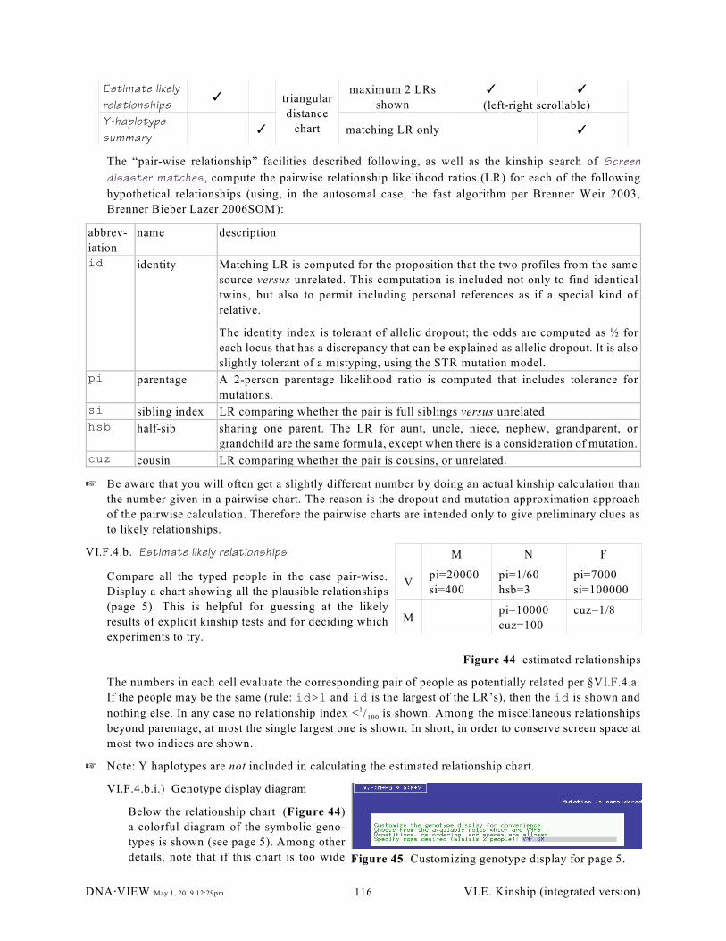
M N F
Vpi=20000
si=400
pi=1/60
hsb=3
pi=7000
si=100000
Mpi=10000
cuz=100
cuz=1/8
Figure 44 estimated relationships
Figure 45 Customizing genotype display for page 5.
Estimate likely
relationshipsT triangular
distance
chart
maximum 2 LRs
shown
T T
(left-right scrollable)
Y-haplotype
summaryT matching LR only T
The “pair-wise relationship” facilities described following, as well as the kinship search of Screen
disaster matches , compute the pairwise relationship likelihood ratios (LR) for each of the following
hypothetical relationships (using, in the autosomal case, the fast algorithm per Brenner Weir 2003,
Brenner Bieber Lazer 2006SOM):
abbrev-
iation
name description
id identity Matching LR is computed for the proposition that the two profiles from the same
source versus unrelated. This computation is included not only to find identical
twins, but also to permit including personal references as if a special kind of
relative.
The identity index is tolerant of allelic dropout; the odds are computed as ½ for
each locus that has a discrepancy that can be explained as allelic dropout. It is also
slightly tolerant of a mistyping, using the STR mutation model.
pi parentage A 2-person parentage likelihood ratio is computed that includes tolerance for
mutations.
si sibling index LR comparing whether the pair is full siblings versus unrelated
hsb half-sib sharing one parent. The LR for aunt, uncle, niece, nephew, grandparent, or
grandchild are the same formula, except when there is a consideration of mutation.
cuz cousin LR comparing whether the pair is cousins, or unrelated.
L Be aware that you will often get a slightly different number by doing an actual kinship calculation than
the number given in a pairwise chart. The reason is the dropout and mutation approximation approach
of the pairwise calculation. Therefore the pairwise charts are intended only to give preliminary clues as
to likely relationships.
VI.F.4.b. Estimate likely relationships
Compare all the typed people in the case pair-wise.
Display a chart showing all the plausible relationships
(page 5). This is helpful for guessing at the likely
results of explicit kinship tests and for deciding which
experiments to try.
The numbers in each cell evaluate the corresponding pair of people as potentially related per §VI.F.4.a.
If the people may be the same (rule: id>1 and id is the largest of the LR’s), then the id is shown and
100nothing else. In any case no relationship index < / is shown. Among the miscellaneous relationships1
beyond parentage, at most the single largest one is shown. In short, in order to conserve screen space at
most two indices are shown.
L Note: Y haplotypes are not included in calculating the estimated relationship chart.
VI.F.4.b.i.) Genotype display diagram
Below the relationship chart (Figure 44)
a colorful diagram of the symbolic geno-
types is shown (see page 5). Among other
details, note that if this chart is too wide
DNA@VIEW May 1, 2019 12:29pm VI.E. Kinship (integrated version)116
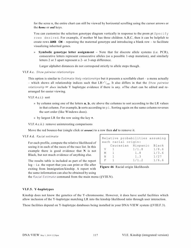
Relative probabilities assumingeach racial origin: Caucasian Hispanic Black V 1 1/1.8 1/8.6 M 1 1.8 1/3.6 N 1 1.3 1/27 F 1 1/1.2 1/6.6
Figure 46 Racial origin likelihoods
for the scree n, the entire chart can still be viewed by horizontal scrolling using the cursor arrows or
the home or end keys.
You can customize the selection genotype diagram vertically in response to the prom pt Specify
rows desired. For example, if mother M has three children A,B,C, then it can be helpfult to
create rows AMB CM – repeating the maternal genotype and introducing a blank row – to facilitate
visualizing inherited genes.
» Symbolic genotype letter assignment – Note that for discrete allele systems (i.e. PCR),
consecutive letters represent consecutive alleles (so a possible 1-step mutation), and similarly
letters 2 or 3 apart represent a 2- or 3-step difference.
Larger alphabet distances do not correspond strictly to allele steps though.
VI.F.4.c. Show pairwise relationships
This option is similar to Estimate likely relationships but it presents a scrollable chart – a menu actually
100– which shows all relationship indices such that LR> / . It also differs in that the Show pairwise1
relationship L does include Y haplotype evidence if there is any. nThe chart can be edited and re-
arranged for easier viewing.
VI.F.4.c.i.) sort
» by column using one of the letters a, b, etc above the columns to sort according to the LR values
in that column. For example, b sorts according to pi. Sorting again on the same column reverses
the sort order (like Windows does).
» by largest LR for the row using the key +.
VI.F.4.c.ii.) remove uninteresting comparisons
Move the red bounce-bar (single click or arrow) to a row then del to remove it.
VI.F.4.d. Racial estimate
For each profile, compute the relative likelihood of
seeing it in each of the races of the race list. In this
example there is good evidence that N is not
Black, but not much evidence of anything else.
The results table is included as part of the report
log – i.e. the report that you can print or file after
exiting from Immigration/kinship. A report with
the same information can also be obtained by using
the Racial Estimate command from the main menu (§VIII.N).
VI.F.5. Y-haplotypes
Kinship does not know the genetics of the Y-chromosome. However, it does have useful facilities which
allow inclusion of the Y-haplotype matching LR into the kinship likelihood ratio through user interaction.
These facilities depend on Y-haplotype databases being installed in your DNA@VIEW system (§VIII.F.3).
DNA@VIEW May 1, 2019 12:29pm VI.E. Kinship (integrated version)117
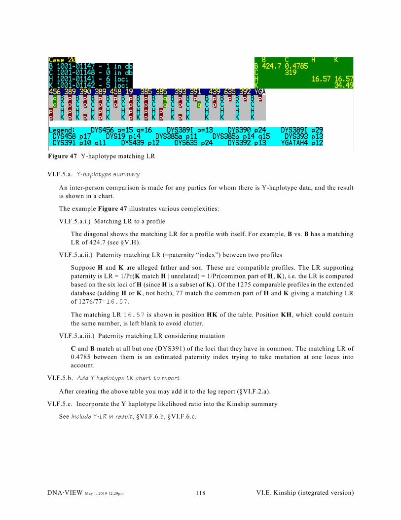
Figure 47 Y-haplotype matching LR
VI.F.5.a. Y-haplotype summary
An inter-person comparison is made for any parties for whom there is Y-haplotype data, and the result
is shown in a chart.
The example Figure 47 illustrates various complexities:
VI.F.5.a.i.) Matching LR to a profile
The diagonal shows the matching LR for a profile with itself. For example, B vs. B has a matching
LR of 424.7 (see §V.H).
VI.F.5.a.ii.) Paternity matching LR (=paternity “index”) between two profiles
Suppose H and K are alleged father and son. These are compatible profiles. The LR supporting
paternity is LR = 1/Pr(K match H | unrelated) = 1/Pr(common part of H, K), i.e. the LR is computed
based on the six loci of H (since H is a subset of K). Of the 1275 comparable profiles in the extended
database (adding H or K , not both), 77 match the common part of H and K giving a matching LR
of 1276/77=16.57.
The matching LR 16.57 is shown in position HK of the table. Position KH, which could contain
the same number, is left blank to avoid clutter.
VI.F.5.a.iii.) Paternity matching LR considering mutation
C and B match at all but one (DYS391) of the loci that they have in common. The matching LR of
0.4785 between them is an estimated paternity index trying to take mutation at one locus into
account.
VI.F.5.b. Add Y haplotype LR chart to report
After creating the above table you may add it to the log report (§VI.F.2.a).
VI.F.5.c. Incorporate the Y haplotype likelihood ratio into the Kinship summary
See Include Y-LR in result, §VI.F.6.b, §VI.F.6.c.
DNA@VIEW May 1, 2019 12:29pm VI.E. Kinship (integrated version)118
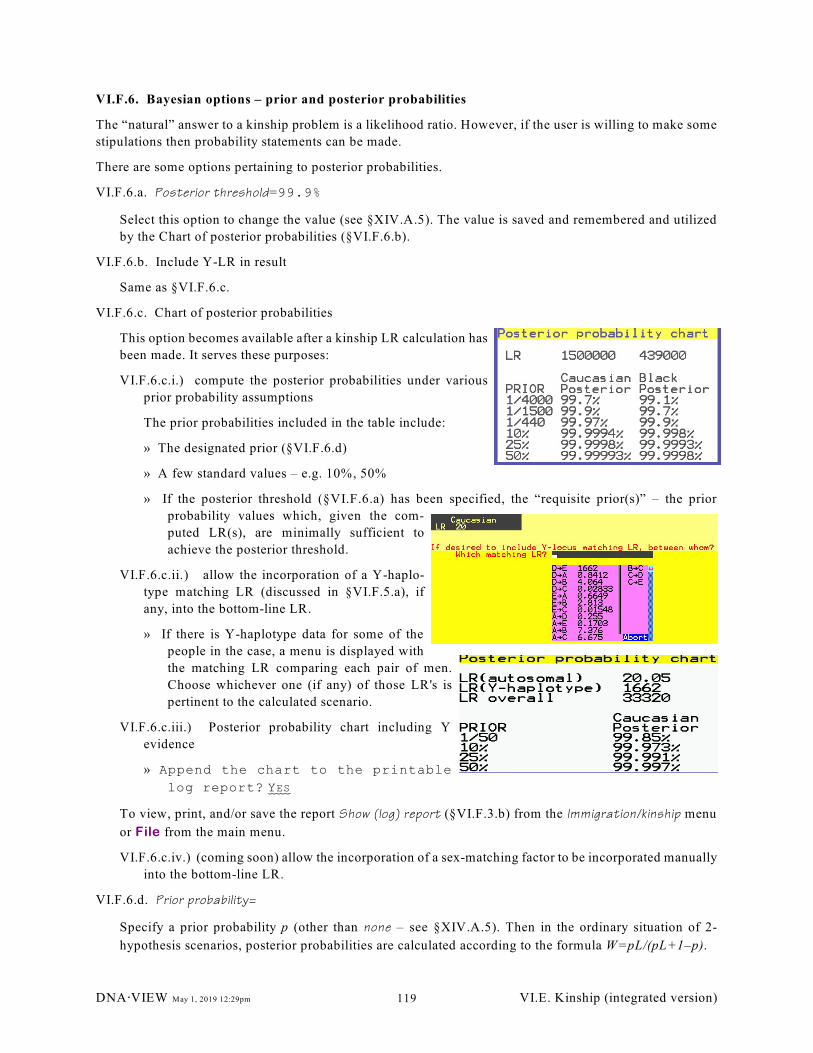
VI.F.6. Bayesian options – prior and posterior probabilities
The “natural” answer to a kinship problem is a likelihood ratio. However, if the user is willing to make some
stipulations then probability statements can be made.
There are some options pertaining to posterior probabilities.
VI.F.6.a. Posterior threshold=99.9%
Select this option to change the value (see §XIV.A.5). The value is saved and remembered and utilized
by the Chart of posterior probabilities (§VI.F.6.b).
VI.F.6.b. Include Y-LR in result
Same as §VI.F.6.c.
VI.F.6.c. Chart of posterior probabilities
This option becomes available after a kinship LR calculation has
been made. It serves these purposes:
VI.F.6.c.i.) compute the posterior probabilities under various
prior probability assumptions
The prior probabilities included in the table include:
» The designated prior (§VI.F.6.d)
» A few standard values – e.g. 10%, 50%
» If the posterior threshold (§VI.F.6.a) has been specified, the “requisite prior(s)” – the prior
probability values which, given the com-
puted LR(s), are minimally sufficient to
achieve the posterior threshold.
VI.F.6.c.ii.) allow the incorporation of a Y-haplo-
type matching LR (discussed in §VI.F.5.a), if
any, into the bottom-line LR.
» If there is Y-haplotype data for some of the
people in the case, a menu is displayed with
the matching LR comparing each pair of men.
Choose whichever one (if any) of those LR's is
pertinent to the calculated scenario.
VI.F.6.c.iii.) Posterior probability chart including Y
evidence
» Append the chart to the printable
log report? YES
To view, print, and/or save the report Show (log) report (§VI.F.3.b) from the Immigration/kinship menu
or File from the main menu.
VI.F.6.c.iv.) (coming soon) allow the incorporation of a sex-matching factor to be incorporated manually
into the bottom-line LR.
VI.F.6.d. Prior probability=
Specify a prior probability p (other than none – see §XIV.A.5). Then in the ordinary situation of 2-
hypothesis scenarios, posterior probabilities are calculated according to the formula W=pL/(pL+1–p).
DNA@VIEW May 1, 2019 12:29pm VI.E. Kinship (integrated version)119
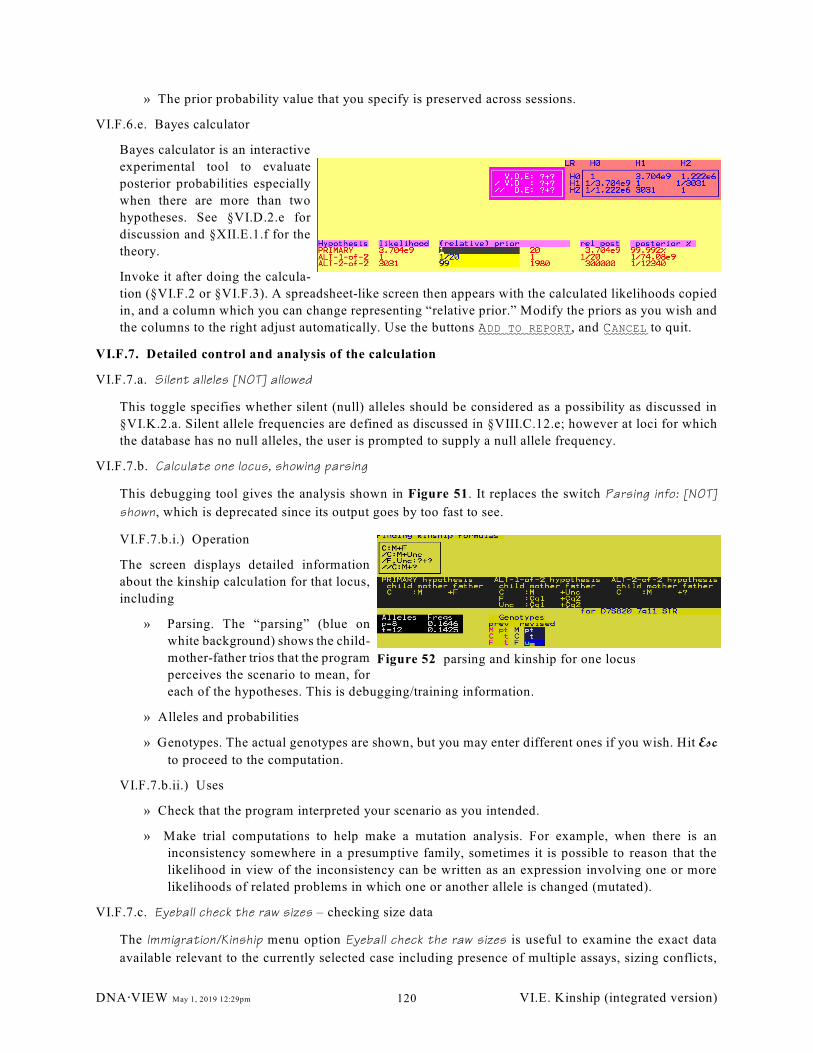
Figure 52 parsing and kinship for one locus
» The prior probability value that you specify is preserved across sessions.
VI.F.6.e. Bayes calculator
Bayes calculator is an interactive
experimental tool to evaluate
posterior probabilities especially
when there are more than two
hypotheses. See §VI.D.2.e for
discussion and §XII.E.1.f for the
theory.
Invoke it after doing the calcula-
tion (§VI.F.2 or §VI.F.3). A spreadsheet-like screen then appears with the calculated likelihoods copied
in, and a column which you can change representing “relative prior.” Modify the priors as you wish and
the columns to the right adjust automatically. Use the buttons ADD TO REPORT, and CANCEL to quit.
VI.F.7. Detailed control and analysis of the calculation
VI.F.7.a. Silent alleles [NOT] allowed
This toggle specifies whether silent (null) alleles should be considered as a possibility as discussed in
§VI.K.2.a. Silent allele frequencies are defined as discussed in §VIII.C.12.e; however at loci for which
the database has no null alleles, the user is prompted to supply a null allele frequency.
VI.F.7.b. Calculate one locus, showing parsing
This debugging tool gives the analysis shown in Figure 51. It replaces the switch Parsing info: [NOT]
shown, which is deprecated since its output goes by too fast to see.
VI.F.7.b.i.) Operation
The screen displays detailed information
about the kinship calculation for that locus,
including
» Parsing. The “parsing” (blue on
white background) shows the child-
mother-father trios that the program
perceives the scenario to mean, for
each of the hypotheses. This is debugging/training information.
» Alleles and probabilities
» Genotypes. The actual genotypes are shown, but you may enter different ones if you wish. Hit Esc
to proceed to the computation.
VI.F.7.b.ii.) Uses
» Check that the program interpreted your scenario as you intended.
» Make trial computations to help make a mutation analysis. For example, when there is an
inconsistency somewhere in a presumptive family, sometimes it is possible to reason that the
likelihood in view of the inconsistency can be written as an expression involving one or more
likelihoods of related problems in which one or another allele is changed (mutated).
VI.F.7.c. Eyeball check the raw sizes – checking size data
The Immigration/Kinship menu option Eyeball check the raw sizes is useful to examine the exact data
available relevant to the currently selected case including presence of multiple assays, sizing conflicts,
DNA@VIEW May 1, 2019 12:29pm VI.E. Kinship (integrated version)120
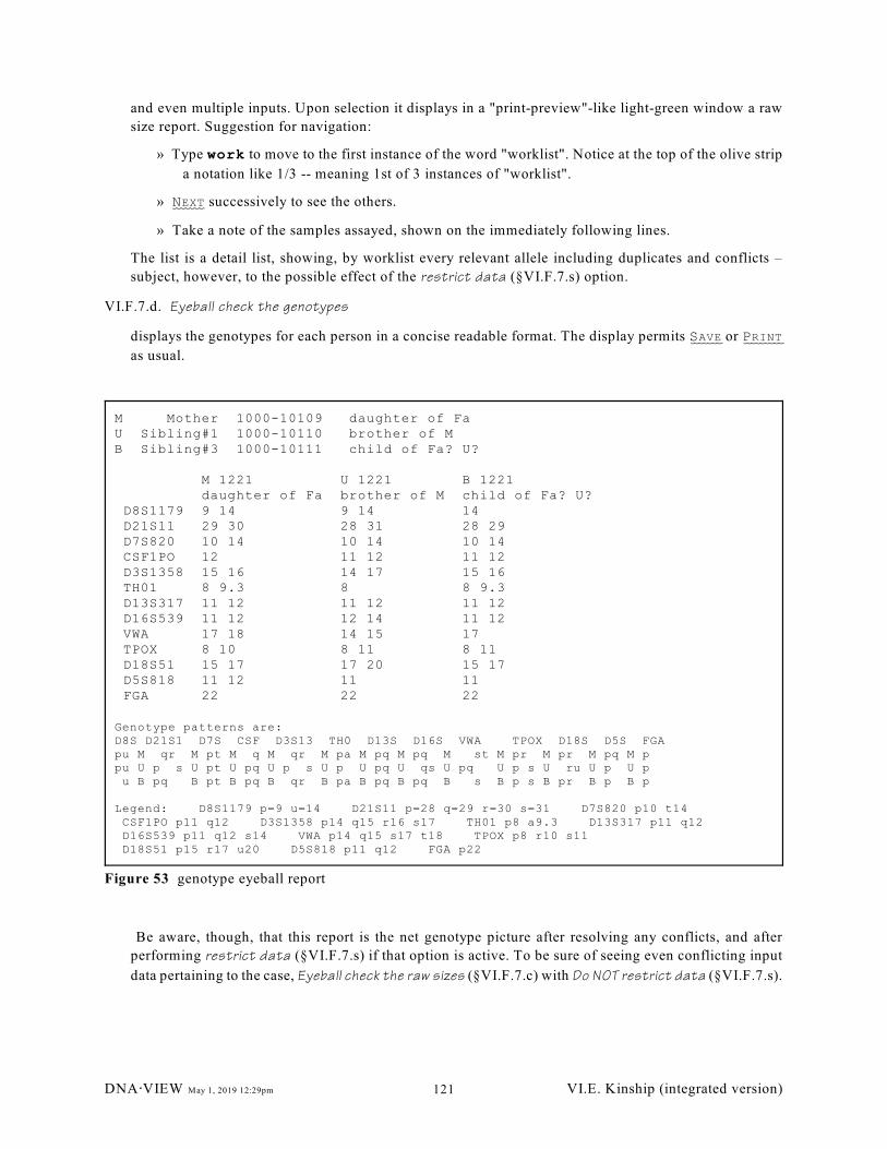
M Mother 1000-10109 daughter of FaU Sibling#1 1000-10110 brother of MB Sibling#3 1000-10111 child of Fa? U?
M 1221 U 1221 B 1221 daughter of Fa brother of M child of Fa? U? D8S1179 9 14 9 14 14 D21S11 29 30 28 31 28 29 D7S820 10 14 10 14 10 14 CSF1PO 12 11 12 11 12 D3S1358 15 16 14 17 15 16 TH01 8 9.3 8 8 9.3 D13S317 11 12 11 12 11 12 D16S539 11 12 12 14 11 12 VWA 17 18 14 15 17 TPOX 8 10 8 11 8 11 D18S51 15 17 17 20 15 17 D5S818 11 12 11 11 FGA 22 22 22
Genotype patterns are:D8S D21S1 D7S CSF D3S13 TH0 D13S D16S VWA TPOX D18S D5S FGApu M qr M pt M q M qr M pa M pq M pq M st M pr M pr M pq M ppu U p s U pt U pq U p s U p U pq U qs U pq U p s U ru U p U p u B pq B pt B pq B qr B pa B pq B pq B s B p s B pr B p B p
Legend: D8S1179 p=9 u=14 D21S11 p=28 q=29 r=30 s=31 D7S820 p10 t14 CSF1PO p11 q12 D3S1358 p14 q15 r16 s17 TH01 p8 a9.3 D13S317 p11 q12 D16S539 p11 q12 s14 VWA p14 q15 s17 t18 TPOX p8 r10 s11 D18S51 p15 r17 u20 D5S818 p11 q12 FGA p22
Figure 53 genotype eyeball report
and even multiple inputs. Upon selection it displays in a "print-preview"-like light-green window a raw
size report. Suggestion for navigation:
» Type work to move to the first instance of the word "worklist". Notice at the top of the olive strip
a notation like 1/3 -- meaning 1st of 3 instances of "worklist".
» NEXT successively to see the others.
» Take a note of the samples assayed, shown on the immediately following lines.
The list is a detail list, showing, by worklist every relevant allele including duplicates and conflicts –
subject, however, to the possible effect of the restrict data (§VI.F.7.s) option.
VI.F.7.d. Eyeball check the genotypes
displays the genotypes for each person in a concise readable format. The display permits SAVE or PRINT
as usual.
Be aware, though, that this report is the net genotype picture after resolving any conflicts, and after
performing restrict data (§VI.F.7.s) if that option is active. To be sure of seeing even conflicting input
data pertaining to the case, Eyeball check the raw sizes (§VI.F.7.c) with Do NOT restrict data (§VI.F.7.s).
DNA@VIEW May 1, 2019 12:29pm VI.E. Kinship (integrated version)121
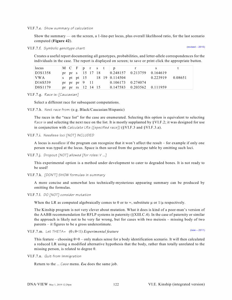
VI.F.7.e. Show summary of calculation
Show the summary — on the screen, a 1-line-per locus, plus overall likelihood ratio, for the last scenario
computed (Figure 42).
VI.F.7.f. Symbolic genotype chart (revised – 2010)
Creates a useful report documenting all genotypes, probabilities, and letter-allele correspondences for the
individuals in the case. The report is displayed on screen; to save or print click the appropriate button.
locus M C F p r s t p r s t
D3S1358 pr pr s 15 17 18 0.248157 0.213759 0.164619
VWA s pt pt 15 18 19 0.114504 0.223919 0.08651
D16S539 pr pr pr 9 11 0.106173 0.274074
D8S1179 pr pr rs 12 14 15 0.147583 0.203562 0.111959
VI.F.7.g. Race is: [Caucasian]
Select a different race for subsequent computations.
VI.F.7.h. Next race from: (e.g. Black/Caucasian/Hispanic)
The races in the “race list” for the case are enumerated. Selecting this option is equivalent to selecting
Race is and selecting the next race on the list. It is mostly supplanted by §VI.F.2; it was designed for use
in conjunction with Calculate LRs ([specified race]) (§VI.F.3 and §VI.F.3.a).
VI.F.7.i. Needless loci [NOT] INCLUDED
A locus is needless if the program can recognize that it won’t affect the result – for example if only one
person was typed at the locus. Space is then saved from the genotype table by omitting such loci.
VI.F.7.j. Dropout [NOT] allowed [for roles: V ...]
This experimental option is a method under development to cater to degraded bones. It is not ready to
be used!
VI.F.7.k. [DON’T] SHOW formulas in summary
A more concise and somewhat less technically-mysterious appearing summary can be produced by
omitting the formulas.
VI.F.7.l. DO [NOT] consider mutation
When the LR as computed algebraically comes to 0 or to 4, substitute ì or 1/ì respectively.
The Kinship program is not very clever about mutation. What it does is kind of a poor-man’s version of
the AABB recommendation for RFLP systems in paternity (§XIII.C.4). In the case of paternity or similar
the approach is likely not to be very far wrong, but for cases with two meiosis – missing body of two
parents – it figures to be a gross underestimate.
VI.F.7.m. Let THETA= (0#è<1) Experimental feature (new – 2011)
This feature – choosing è>0 – only makes sense for a body identification scenario. It will then calculated
a reduced LR using a modified alternative hypothesis that the body, rather than totally unrelated to the
missing person, is related to degree è.
VI.F.7.n. Quit from Immigration
Return to the ... Case menu. Esc does the same job.
DNA@VIEW May 1, 2019 12:29pm VI.E. Kinship (integrated version)122
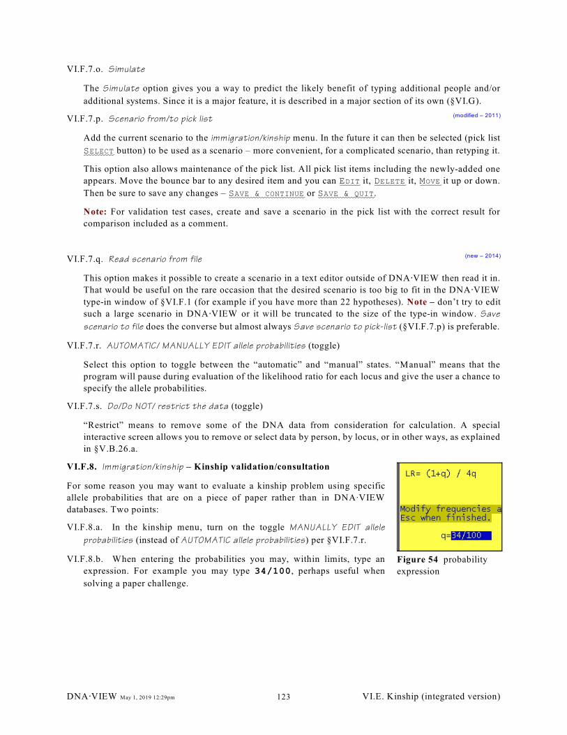
Figure 54 probability
expression
VI.F.7.o. Simulate
The Simulate option gives you a way to predict the likely benefit of typing additional people and/or
additional systems. Since it is a major feature, it is described in a major section of its own (§VI.G).
VI.F.7.p. Scenario from/to pick list (modified – 2011)
Add the current scenario to the immigration/kinship menu. In the future it can then be selected (pick list
SELECT button) to be used as a scenario – more convenient, for a complicated scenario, than retyping it.
This option also allows maintenance of the pick list. All pick list items including the newly-added one
appears. Move the bounce bar to any desired item and you can EDIT it, DELETE it, MOVE it up or down.
Then be sure to save any changes – SAVE & CONTINUE or SAVE & QUIT.
Note: For validation test cases, create and save a scenario in the pick list with the correct result for
comparison included as a comment.
VI.F.7.q. Read scenario from file (new – 2014)
This option makes it possible to create a scenario in a text editor outside of DNA@VIEW then read it in.
That would be useful on the rare occasion that the desired scenario is too big to fit in the DNA@VIEW
type-in window of §VI.F.1 (for example if you have more than 22 hypotheses). Note – don’t try to edit
such a large scenario in DNA@VIEW or it will be truncated to the size of the type-in window. Save
scenario to file does the converse but almost always Save scenario to pick-list (§VI.F.7.p) is preferable.
VI.F.7.r. AUTOMATIC/ MANUALLY EDIT allele probabilities (toggle)
Select this option to toggle between the “automatic” and “manual” states. “Manual” means that the
program will pause during evaluation of the likelihood ratio for each locus and give the user a chance to
specify the allele probabilities.
VI.F.7.s. Do/Do NOT/ restrict the data (toggle)
“Restrict” means to remove some of the DNA data from consideration for calculation. A special
interactive screen allows you to remove or select data by person, by locus, or in other ways, as explained
in §V.B.26.a.
VI.F.8. Immigration/kinship – Kinship validation/consultation
For some reason you may want to evaluate a kinship problem using specific
allele probabilities that are on a piece of paper rather than in DNAAVIEW
databases. Two points:
VI.F.8.a. In the kinship menu, turn on the toggle MANUALLY EDIT allele
probabilities (instead of AUTOMATIC allele probabilities) per §VI.F.7.r.
VI.F.8.b. When entering the probabilities you may, within limits, type an
expression. For example you may type 34/100, perhaps useful when
solving a paper challenge.
DNA@VIEW May 1, 2019 12:29pm VI.E. Kinship (integrated version)123
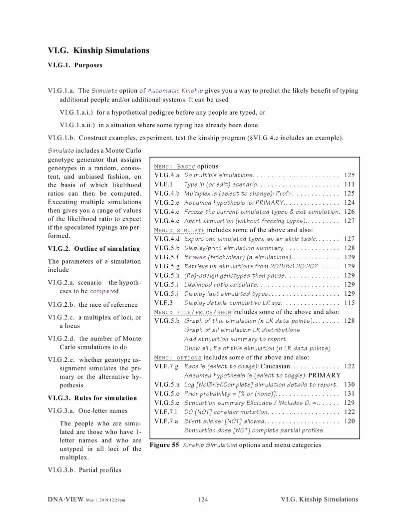
MENU: BASIC options
VI.G.4.a Do multiple simulations. . . . . . . . . . . . . . . . . . . . . . . . 125
VI.F.1 Type in (or edit) scenario. . . . . . . . . . . . . . . . . . . . . . . 111
VI.G.4.b Multiplex is (select to change): Prof+. . . . . . . . . . . . . 125
VI.G.2.e Assumed hypothesis is: PRIMARY. . . . . . . . . . . . . . . . 124
VI.G.4.c Freeze the current simulated types & exit simulation. 126
VI.G.4.e Abort simulation (without freezing types). . . . . . . . . . 127
MENU: SIMULATE includes some of the above and also:
VI.G.4.d Export the simulated types as an allele table. . . . . . . 127
VI.G.5.b Display/print simulation summary. . . . . . . . . . . . . . . . 128
VI.G.5.f Browse (fetch/clear) (n simulations). . . . . . . . . . . . . . 129
VI.G.5.g Retrieve nn simulations from 2011/8/1 20:20?. . . . . . 129
VI.G.5.h (Re)-assign genotypes then pause. . . . . . . . . . . . . . . 129
VI.G.5.i Likelihood ratio calculate. . . . . . . . . . . . . . . . . . . . . . . 129
VI.G.5.j Display last simulated types. . . . . . . . . . . . . . . . . . . . 129
VI.F.3 Display details cumulative LR xyz. . . . . . . . . . . . . . . . 115
MENU: FILE/FETCH/SHOW includes some of the above and also:
VI.G.5.b Graph of this simulation (n LR data points). . . . . . . . 128
Graph of all simulation LR distributions
Add simulation summary to report
Show all LRs of this simulation (n LR data points)
MENU: OPTIONS includes some of the above and also:
VI.F.7.g Race is (select to chage): Caucasian. . . . . . . . . . . . . . 122
Assumed hypothesis is (select to toggle): PRIMARY
VI.G.5.n Log [No|Brief|Complete] simulation details to report. 130
VI.G.5.o Prior probability = [% or (none)]. . . . . . . . . . . . . . . . . . 131
VI.G.5.e Simulation summary EXcludes / INcludes 0, 4.. . . . . . 129
VI.F.7.l DO [NOT] consider mutation. . . . . . . . . . . . . . . . . . . . 122
VI.F.7.a Silent alleles: [NOT] allowed. . . . . . . . . . . . . . . . . . . . . 120
Simulation does [NOT] complete partial profiles
Figure 55 Kinship Simulation options and menu categories
VI.G. Kinship Simulations
VI.G.1. Purposes
VI.G.1.a. The Simulate option of Automatic Kinship gives you a way to predict the likely benefit of typing
additional people and/or additional systems. It can be used
VI.G.1.a.i.) for a hypothetical pedigree before any people are typed, or
VI.G.1.a.ii.) in a situation where some typing has already been done.
VI.G.1.b. Construct examples, experiment, test the kinship program (§VI.G.4.c includes an example).
Simulate includes a Monte Carlo
genotype generator that assigns
genotypes in a random, consis-
tent, and unbiased fashion, on
the basis of which likelihood
ratios can then be computed.
Executing multiple simulations
then gives you a range of values
of the likelihood ratio to expect
if the speculated typings are per-
formed.
VI.G.2. Outline of simulating
The parameters of a simulation
include
VI.G.2.a. scenario – the hypoth-
eses to be compared
VI.G.2.b. the race of reference
VI.G.2.c. a multiplex of loci, or
a locus
VI.G.2.d. the number of Monte
Carlo simulations to do
VI.G.2.e. whether genotype as-
signment simulates the pri-
mary or the alternative hy-
pothesis
VI.G.3. Rules for simulation
VI.G.3.a. One-letter names
The people who are simu-
lated are those who have 1-
letter names and who are
untyped in all loci of the
multiplex.
VI.G.3.b. Partial profiles
DNA@VIEW May 1, 2019 12:29pm VI.G. Kinship Simulations124
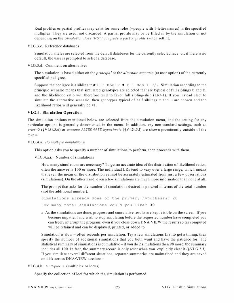
Real profiles or partial profiles may exist for some roles (=people with 1-letter names) in the specified
multiplex. They are used, not discarded. A partial profile may or be filled in by the simulation or not
depending on the Simulation does [NOT] complete a partial profile switch setting.
VI.G.3.c. Reference databases
Simulation alleles are selected from the default databases for the currently selected race; or, if there is no
default, the user is prompted to select a database.
VI.G.3.d. Comment on alternatives
The simulation is based either on the principal or the alternate scenario (at user option) of the currently
specified pedigree.
Suppose the pedigree is a sibling test: C : Mom+F Ë D : Mom + F/?. Simulation according to the
principle scenario means that simulated genotypes are selected that are typical of full siblings C and D,
and the likelihood ratio will therefore tend to favor full sibling-ship (LR>1). If you instead elect to
simulate the alternative scenario, then genotypes typical of half siblings C and D are chosen and the
likelihood ratios will generally be <1.
VI.G.4. Simulation Operation
The simulation options mentioned below are selected from the simulation menu, and the setting for any
particular options is generally documented in the menu. In addition, any non-standard settings, such as
prior>0 (§VI.G.5.o) or assume ALTERNATE hypothesis (§VI.G.5.l) are shown prominently outside of the
menu.
VI.G.4.a. Do multiple simulations
This option asks you to specify a number of simulations to perform, then proceeds with them.
VI.G.4.a.i.) Number of simulations
How many simulations are necessary? To get an accurate idea of the distribution of likelihood ratios,
often the answer is 100 or more. The individual LRs tend to vary over a large range, which means
that even the mean of the distribution cannot be accurately estimated from just a few observations
(simulations). On the other hand, even a few simulations are much more information than none at all.
The prompt that asks for the number of simulations desired is phrased in terms of the total number
(not the additional number).
Simulations already done of the primary hypothesis: 20
How many total simulations would you like? 30
» As the simulations are done, progress and cumulative results are kept visible on the screen. If you
become impatient and wish to stop simulating before the requested number have completed you
can freely interrupt the program; even if you close down DNAAVIEW the results so far computed
will be retained and can be displayed, printed, or added to.
Simulation is slow – often seconds per simulation. Try a few simulations first to get a timing, then
specify the number of additional simulations that you both want and have the patience for. The
statistical summary of simulations is cumulative – if you do 2 simulations then 98 more, the summary
includes all 100. In fact, the summary record is only reset when you explicitly clear it (§VI.G.5.f).
If you simulate several different situations, separate summaries are maintained and they are saved
on disk across DNA@VIEW sessions.
VI.G.4.b. Multiplex is: (multiplex or locus)
Specify the collection of loci for which the simulation is performed.
DNA@VIEW May 1, 2019 12:29pm VI.G. Kinship Simulations125
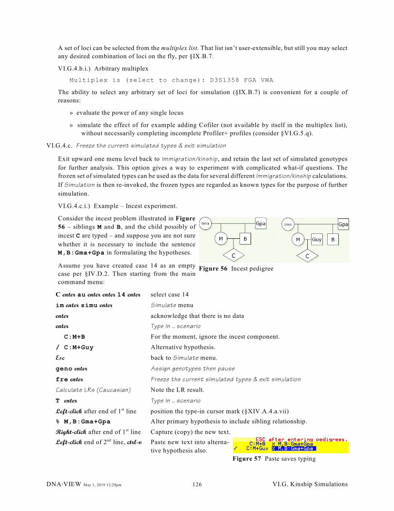
Figure 56 Incest pedigree
Figure 57 Paste saves typing
A set of loci can be selected from the multiplex list. That list isn’t user-extensible, but still you may select
any desired combination of loci on the fly, per §IX.B.7.
VI.G.4.b.i.) Arbitrary multiplex
Multiplex is (select to change): D3S1358 FGA VWA
The ability to select any arbitrary set of loci for simulation (§IX.B.7) is convenient for a couple of
reasons:
» evaluate the power of any single locus
» simulate the effect of for example adding Cofiler (not available by itself in the multiplex list),
without necessarily completing incomplete Profiler+ profiles (consider §VI.G.5.q).
VI.G.4.c. Freeze the current simulated types & exit simulation
Exit upward one menu level back to Immigration/kinship, and retain the last set of simulated genotypes
for further analysis. This option gives a way to experiment with complicated what-if questions. The
frozen set of simulated types can be used as the data for several different Immigration/kinship calculations.
If Simulation is then re-invoked, the frozen types are regarded as known types for the purpose of further
simulation.
VI.G.4.c.i.) Example – Incest experiment.
Consider the incest problem illustrated in Figure
56 – siblings M and B, and the child possibly of
incest C are typed – and suppose you are not sure
whether it is necessary to include the sentence
M,B:Gma+Gpa in formulating the hypotheses.
Assume you have created case 14 as an empty
case per §IV.D.2. Then starting from the main
command menu:
C enter au enter enter 14 enter select case 14
im enter simu enter Simulate menu
enter acknowledge that there is no data
enter Type in .. scenario
C:M+B For the moment, ignore the incest component.
/ C:M+Guy Alternative hypothesis.
Esc back to Simulate menu.
geno enter Assign genotypes then pause
fre enter Freeze the current simulated types & exit simulation
Calculate LRs (Caucasian) Note the LR result.
T enter Type in .. scenario
Left-click after end of 1 line position the type-in cursor mark (§XIV.A.4.a.vii)st
% M,B:Gma+Gpa Alter primary hypothesis to include sibling relationship.
Right-click after end of 1 line Capture (copy) the new text.st
Left-click end of 2 line, ctrl-v Paste new text into alterna-nd
tive hypothesis also.
DNA@VIEW May 1, 2019 12:29pm VI.G. Kinship Simulations126
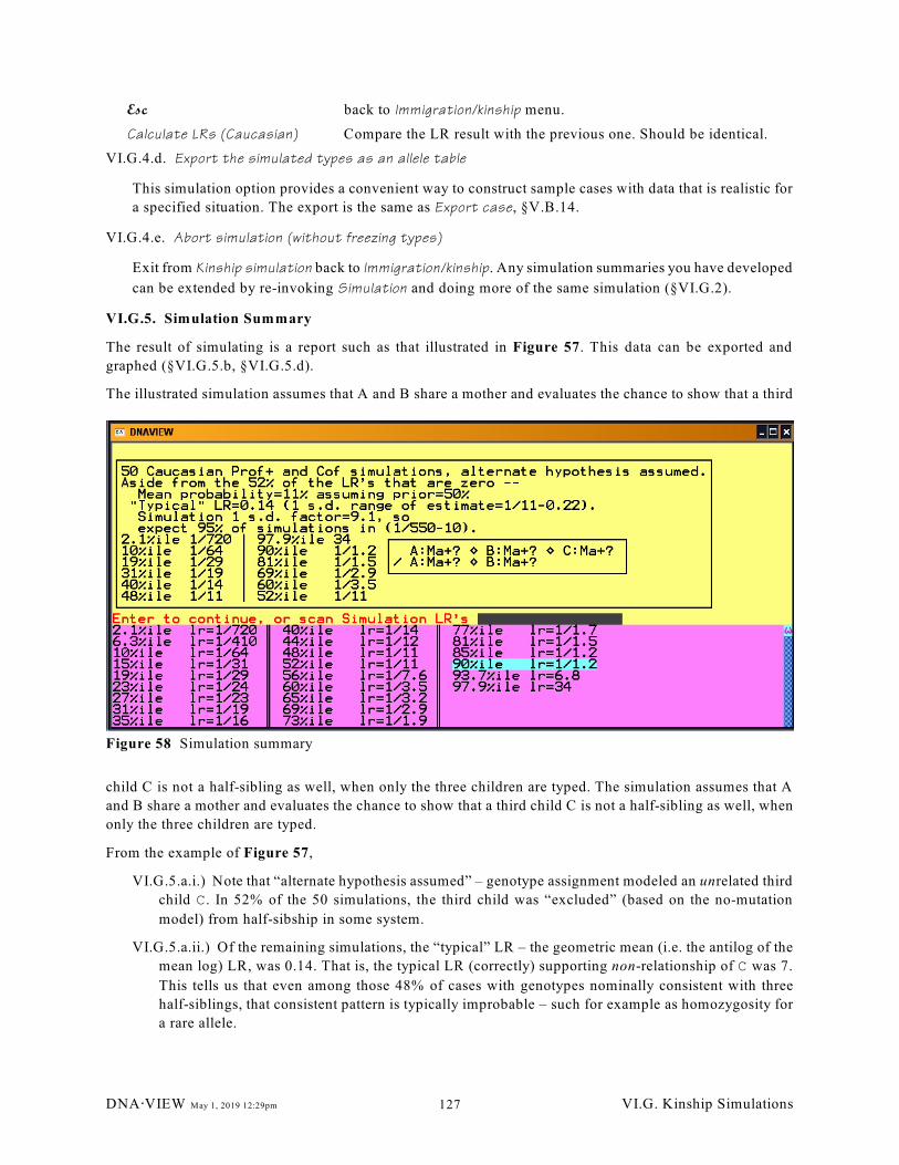
Figure 58 Simulation summary
Esc back to Immigration/kinship menu.
Calculate LRs (Caucasian) Compare the LR result with the previous one. Should be identical.
VI.G.4.d. Export the simulated types as an allele table
This simulation option provides a convenient way to construct sample cases with data that is realistic for
a specified situation. The export is the same as Export case, §V.B.14.
VI.G.4.e. Abort simulation (without freezing types)
Exit from Kinship simulation back to Immigration/kinship. Any simulation summaries you have developed
can be extended by re-invoking Simulation and doing more of the same simulation (§VI.G.2).
VI.G.5. Simulation Summary
The result of simulating is a report such as that illustrated in Figure 57. This data can be exported and
graphed (§VI.G.5.b, §VI.G.5.d).
The illustrated simulation assumes that A and B share a mother and evaluates the chance to show that a third
child C is not a half-sibling as well, when only the three children are typed. The simulation assumes that A
and B share a mother and evaluates the chance to show that a third child C is not a half-sibling as well, when
only the three children are typed.
From the example of Figure 57,
VI.G.5.a.i.) Note that “alternate hypothesis assumed” – genotype assignment modeled an unrelated third
child C. In 52% of the 50 simulations, the third child was “excluded” (based on the no-mutation
model) from half-sibship in some system.
VI.G.5.a.ii.) Of the remaining simulations, the “typical” LR – the geometric mean (i.e. the antilog of the
mean log) LR, was 0.14. That is, the typical LR (correctly) supporting non-relationship of C was 7.
This tells us that even among those 48% of cases with genotypes nominally consistent with three
half-siblings, that consistent pattern is typically improbable – such for example as homozygosity for
a rare allele.
DNA@VIEW May 1, 2019 12:29pm VI.G. Kinship Simulations127
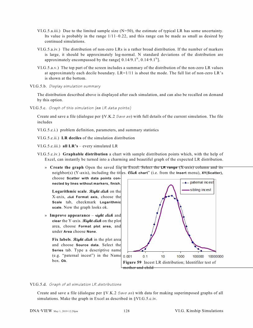
Figure 59 Incest LR distribution; Identifiler test of
mother and child
VI.G.5.a.iii.) Due to the limited sample size (N=50), the estimate of typical LR has some uncertainty.
Its value is probably in the range 1/11–0.22, and this range can be made as small as desired by
continued simulations.
VI.G.5.a.iv.) The distribution of non-zero LRs is a rather broad distribution. If the number of markers
is large, it should be approximately log-normal. N standard deviations of the distribution are
approximately encompassed by the range[ 0.14/9.1 , [email protected] ].N N
VI.G.5.a.v.) The top part of the screen includes a summary of the distribution of the non-zero LR values
at approximately each decile boundary. LR=1/11 is about the mode. The full list of non-zero LR’s
is shown at the bottom.
VI.G.5.b. Display simulation summary
The distribution described above is displayed after each simulation, and can also be recalled on demand
by this option.
VI.G.5.c. Graph of this simulation (nn LR data points)
Create and save a file (dialogue per §V.K.2 Save as) with full details of the current simulation. The file
includes
VI.G.5.c.i.) problem definition, parameters, and summary statistics
VI.G.5.c.ii.) LR deciles of the simulation distribution
VI.G.5.c.iii.) all LR’s – every simulated LR
VI.G.5.c.iv.) Graphable distribution a chart with sample distribution points which, with the help of
Excel, can instantly be turned into a charming and beautiful graph of the expected LR distribution.
» Create the graph Open the saved file in Excel. Select the LR range (X-axis) column and its
neighbor(s) (Y-axis), including the titles. Click chart” (i.e. from the Insert menu), XY(Scatter),
choose Scatter with data points con-
nected by lines without markers, finish.
Logarithmic scale. Right click on the
X-axis, click Format axis, choose the
Scale tab, checkmark Logarithmic
scale. Now the graph looks ok.
» Improve appearance – right click and
clear the Y-axis. Right click on the plot
area, choose Format plot area, and
under Area choose None.
Fix labels. Right click in the plot area
and choose Source data. Select the
Series tab. Type a descriptive name
(e.g. “paternal incest”) in the Name
box. Ok.
VI.G.5.d. Graph of all simulation LR distributions
Create and save a file (dialogue per §V.K.2 Save as) with data for making superimposed graphs of all
simulations. Make the graph in Excel as described in §VI.G.5.c.iv.
DNA@VIEW May 1, 2019 12:29pm VI.G. Kinship Simulations128
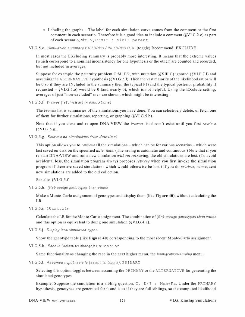
» Labeling the graphs – The label for each simulation curve comes from the comment or the first
comment in each scenario. Therefore it is a good idea to include a comment (§VI.C.2.c) as part
of each scenario, viz: V,C:M+? ; sib+1 parent
VI.G.5.e. Simulation summary EXCLUDES / INCLUDES 0, 4. (toggle) Recommend: EXCLUDE
In most cases the EXcluding summary is probably more interesting. It means that the extreme values
(which correspond to a nominal inconsistency for one hypothesis or the other) are counted and recorded,
but not included in averages.
Suppose for example the paternity problem C:M+F/?, with mutation (§XIII.C) ignored (§VI.F.7.l) and
assuming the ALTERNATIVE hypothesis (§VI.G.5.l). Then the vast majority of the likelihood ratios will
be 0 so if they are INcluded in the summary then the typical PI (and the typical posterior probability if
requested – §VI.G.5.o) would be 0 (and nearly 0), which is not helpful. Using the EXclude setting,
averages of just “non-excluded” men are shown, which might be interesting.
VI.G.5.f. Browse (fetch/clear) (n simulations)
The browse list is summaries of the simulations you have done. You can selectively delete, or fetch one
of them for further simulations, reporting, or graphing (§VI.G.5.b).
Note that if you close and re-open DNA@VIEW the browse list doesn’t exist until you first retrieve
(§VI.G.5.g).
VI.G.5.g. Retrieve nn simulations from date time?
This option allows you to retrieve all the simulations – which can be for various scenarios – which were
last saved on disk on the specified date, time. (The saving is automatic and continuous.) Note that if you
re-start DNA@VIEW and run a new simulation without retrieving, the old simulations are lost. (To avoid
accidental loss, the simulation program always proposes retrieve when you first invoke the simulation
program if there are saved simulations which would otherwise be lost.) If you do retrieve, subsequent
new simulations are added to the old collection.
See also §VI.G.5.f.
VI.G.5.h. (Re)-assign genotypes then pause
Make a Monte-Carlo assignment of genotypes and display them (like Figure 40), without calculating the
LR.
VI.G.5.i. LR calculate
Calculate the LR for the Monte-Carlo assignment. The combination of (Re)-assign genotypes then pause
and this option is equivalent to doing one simulation (§VI.G.4.a).
VI.G.5.j. Display last simulated types
Show the genotype table (like Figure 40) corresponding to the most recent Monte-Carlo assignment.
VI.G.5.k. Race is (select to change): Caucasian
Same functionality as changing the race in the next higher menu, the Immigration/Kinship menu.
VI.G.5.l. Assumed hypothesis is (select to toggle): PRIMARY
Selecting this option toggles between assuming the PRIMARY or the ALTERNATIVE for generating the
simulated genotypes.
Example: Suppose the simulation is a sibling question: C, D/? : Mom+Fa. Under the PRIMARY
hypothesis, genotypes are generated for C and D as if they are full siblings, so the computed likelihood
DNA@VIEW May 1, 2019 12:29pm VI.G. Kinship Simulations129
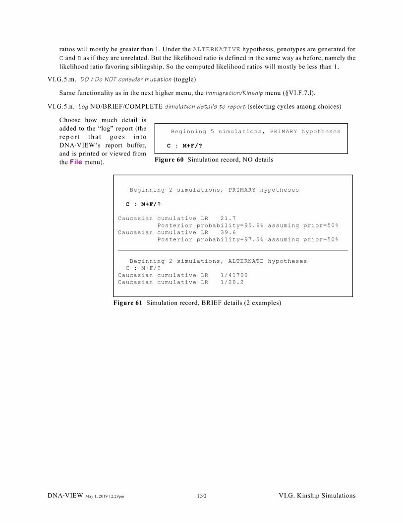
Beginning 5 simulations, PRIMARY hypotheses
C : M+F/?
Figure 60 Simulation record, NO details
Beginning 2 simulations, PRIMARY hypotheses
C : M+F/?
Caucasian cumulative LR 21.7 Posterior probability=95.6% assuming prior=50%Caucasian cumulative LR 39.6 Posterior probability=97.5% assuming prior=50%
Beginning 2 simulations, ALTERNATE hypotheses C : M+F/?Caucasian cumulative LR 1/41700Caucasian cumulative LR 1/20.2
Figure 61 Simulation record, BRIEF details (2 examples)
ratios will mostly be greater than 1. Under the ALTERNATIVE hypothesis, genotypes are generated for
C and D as if they are unrelated. But the likelihood ratio is defined in the same way as before, namely the
likelihood ratio favoring siblingship. So the computed likelihood ratios will mostly be less than 1.
VI.G.5.m. DO / Do NOT consider mutation (toggle)
Same functionality as in the next higher menu, the Immigration/Kinship menu (§VI.F.7.l).
VI.G.5.n. Log NO/BRIEF/COMPLETE simulation details to report (selecting cycles among choices)
Choose how much detail is
added to the “log” report (the
r e p o r t t h a t g o e s in to
DNAAVIEW’s report buffer,
and is printed or viewed from
the File menu).
DNA@VIEW May 1, 2019 12:29pm VI.G. Kinship Simulations130
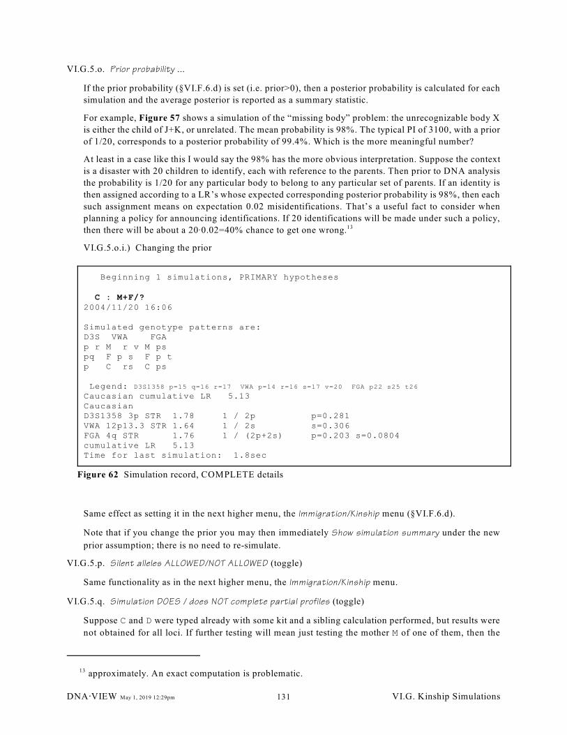
Beginning 1 simulations, PRIMARY hypotheses
C : M+F/?2004/11/20 16:06
Simulated genotype patterns are:D3S VWA FGAp r M r v M pspq F p s F p tp C rs C ps
Legend: D3S1358 p=15 q=16 r=17 VWA p=14 r=16 s=17 v=20 FGA p22 s25 t26Caucasian cumulative LR 5.13CaucasianD3S1358 3p STR 1.78 1 / 2p p=0.281VWA 12p13.3 STR 1.64 1 / 2s s=0.306FGA 4q STR 1.76 1 / (2p+2s) p=0.203 s=0.0804cumulative LR 5.13Time for last simulation: 1.8sec
Figure 62 Simulation record, COMPLETE details
VI.G.5.o. Prior probability ...
If the prior probability (§VI.F.6.d) is set (i.e. prior>0), then a posterior probability is calculated for each
simulation and the average posterior is reported as a summary statistic.
For example, Figure 57 shows a simulation of the “missing body” problem: the unrecognizable body X
is either the child of J+K, or unrelated. The mean probability is 98%. The typical PI of 3100, with a prior
of 1/20, corresponds to a posterior probability of 99.4%. Which is the more meaningful number?
At least in a case like this I would say the 98% has the more obvious interpretation. Suppose the context
is a disaster with 20 children to identify, each with reference to the parents. Then prior to DNA analysis
the probability is 1/20 for any particular body to belong to any particular set of parents. If an identity is
then assigned according to a LR’s whose expected corresponding posterior probability is 98%, then each
such assignment means on expectation 0.02 misidentifications. That’s a useful fact to consider when
planning a policy for announcing identifications. If 20 identifications will be made under such a policy,
then there will be about a 20A0.02=40% chance to get one wrong.13
VI.G.5.o.i.) Changing the prior
Same effect as setting it in the next higher menu, the Immigration/Kinship menu (§VI.F.6.d).
Note that if you change the prior you may then immediately Show simulation summary under the new
prior assumption; there is no need to re-simulate.
VI.G.5.p. Silent alleles ALLOWED/NOT ALLOWED (toggle)
Same functionality as in the next higher menu, the Immigration/Kinship menu.
VI.G.5.q. Simulation DOES / does NOT complete partial profiles (toggle)
Suppose C and D were typed already with some kit and a sibling calculation performed, but results were
not obtained for all loci. If further testing will mean just testing the mother M of one of them, then the
approximately. An exact computation is problematic.13
DNA@VIEW May 1, 2019 12:29pm VI.G. Kinship Simulations131
appropriate simulation assumption would be to NOT complete the partial profiles. However, if it is
proposed to re-test C and D (whether or not M will be simulated), then choose the simulation option DOES
complete.
VI.G.6. Saving simulation scenarios
The history of simulations performed are saved during a session (and NOT LOST when you exit from
DNAAVIEW). Therefore it is possible to do 20 simulations for some scenario, then try a different scenario,
then later return to the first scenario and do 10 further simulations for a total of 30. In order to make it
convenient to return to an earlier scenario the scenarios are included in the “pick list”, which is at the end of
the Immigration/kinship menu.
DNA@VIEW May 1, 2019 12:29pm VI.G. Kinship Simulations132
VI.H. The Prototype Kinship command (stand-alone Kinship program)
Prototype Kinship is the original (1993) kinship program. It is occasionally useful for experiments, such as
to find the formula for a particular genotype pattern. It is stand-alone; it does not directly interact with
DNA@VIEW databases or with people that have been defined as part of a Case or included in a worklist roster.
Therefore for casework it is always easier, faster, and more convenient to use the Automatic Kinship version.
Prototype Kinship analyzes systems consisting of a collection of alleles a, b, ..., n, p , ..., z that exhibit co-
dominance plus possibly one silent allele, which is always designated o. Or, it can analyze X-linked systems.
The result of Prototype Kinship’s calculation is an algebraic formula for the likelihood ratio of the relative
probabilities of the two pedigrees. If you supply the probabilities, it will then evaluate the formula.
VI.I. Kinship cases
Prototype Kinship thus computes one locus at a time. The necessary information for such an analysis is
definitions of the pedigree alternatives, genotype/phenotype information for some or all of the people, and
perhaps probability values for the various genes. For lack of a natural yet descriptive name for this collection
of data, let’s call it a pedigree/locus.
pedigree/locus means the definition for a single locus of a kinship problem, and perhaps additional
associated information including allele probabilities, and the likelihood ratio formula and value.
Part of this data is supplied by the user; part is determined by the program’s computations. The user supplied
part is the script, including symbolic genotype specifications, as describe in §VI.C.
Prototype Kinship also includes some filing and reporting features that enable you to combine computations
across several loci into a unit which is unimaginatively called a complete case
A complete case consists of a collection of pedigree/loci, one for each locus.
Complete cases can be filed and fetched from the a special kinship library in DNA·VIEW and/or PATER with
the
Kinship menu option: File or Fetch a complete case.
A brief locus-by-locus summary of the current complete case can be displayed with the
Kinship menu option: Display Case Summary
Individual pedigree/loci (i.e. for one locus) can be retrieved and re-posted to the current complete case using
the menu options Rework, reorder, or delete a locus and Post this locus to the complete case.
The currently active pedigree/locus can be displayed, edited, or calculated via Display pedigree/locus, Edit
pedigree/locus, Find formula.
Once a formula exists, it is evaluated with Evaluate formula.
Several options are available to construct a report: Clear the report, Insert case summary in the report, Insert
pedigree/locus in the report, Print report (=Print).
DNA@VIEW May 1, 2019 12:29pm VI.H. Prototype Kinship133
VI.J. Overview of using Prototype Kinship
VI.J.1. a new problem
To work through a completely fresh problem, the typical order of operations is:
VI.J.1.a. preparation
Lay out the genotypes for each locus and assign letters in a consistent way to each allele.
VI.J.1.b. Clear complete case
VI.J.1.c. Type in a new pedigree/locus. Recommendation: First, make comment lines with case and locus.
Second, define the genetic types, one line per person, as separate lines. Third, define the relationships.
This format will be easy to modify from locus to locus. It is illustrated in §VI.K.11.
VI.J.1.d. Find formula for locus
VI.J.1.e. Evaluate formula. (Supply relevant allele probabilities as requested.)
VI.J.1.f. Post this locus to the complete case
VI.J.1.f.i.) Post to what row? Select Locus or Serological test or arbitrary as desired.
VI.J.1.f.ii.) Choose a name and the pedigree/locus is posted under that name within the complete case.
VI.J.1.g. File or fetch a complete case. For safety, file the case so far to disk.
VI.J.1.h. Edit pedigree/locus. Modify for the new locus — change the comment & genetic type lines.
Continue from Find formula until all loci are defined. Then prepare a report (§VI.K.13).
VI.J.2. a modified problem
Quite often a kinship problem is a modification — different scenarios for example — of a problem already
worked and filed. The steps in that case are:
VI.J.2.a. preparation (per §VI.J.1.a)
VI.J.2.b. File or fetch a complete case. Retrieve the model that will be modified.
VI.J.2.c. Rework, reorder, or delete a locus
VI.J.2.c.i.) Clear all the old likelihood ratios by moving the red bar to the first locus, then hitting 0 once
per line.
VI.J.2.c.ii.) Select the [next] locus to rework.
VI.J.2.d. Edit pedigree/locus. Change the definition as necessary. Find formula, Evaluate, Post, File (using
a new name) as per the steps in §VI.J.1 above.
Continue from Rework until all loci are defined. Note that the red bounce bars pretty well anticipate what you
want to do — the Rework...locus menu automatically advances one locus at a time, the Post ... locus menu
offers to return the work to the same locus slot from which it came, and the Kinship menu automatically
cycles through the above steps.
When all loci are done, be sure to File (probably to a new complete case name).
Then prepare a report (§VI.K.13).
DNA@VIEW May 1, 2019 12:29pm VI.H. Prototype Kinship134
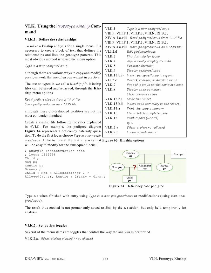
VI.K.1 Type in a new pedigree/locus
VIII.F, VIII.F.1, VIII.F.3, VIII.N, IX.B.3,
XIV.A.4.a.viii Read pedigree/locus from *.KIN file
VIII.F, VIII.F.1, VIII.F.3, VIII.N, IX.B.3,
XIV.A.4.a.viii Save pedigree/locus as a *.KIN file
VI.J.2.d Edit pedigree/locus
VI.K.3 Find formula for locus
VI.K.4 Algebraically simplify formula
VI.K.5 Evaluate formula
VI.K.6 Display pedigree/locus
VI.K.13.b.iv Insert pedigree/locus in report
VI.J.2.c Rework, reorder, or delete a locus
VI.K.7 Post this locus to the complete case
VI.K.8 Display case summary
Clear complete case
VI.K.13.b.i Clear the report
VI.K.13.b.ii Insert case summary in the report
VI.K.13.a Print the case summary
VI.K.10 File or fetch complete case
VI.K.13 Print report (=Print)
quit
VI.K.2.a Silent alleles: not allowed
VI.K.2.b Locus is: autosomal
Figure 63 Kinship options
Figure 64 Deficiency case pedigree
VI.K. Using the Prototype Kinship Com-
mand
VI.K.1. Define the relationships
To make a kinship analysis for a single locus, it is
necessary to create block of text that defines the
relationships and lists the genotype patterns. This
most obvious method is to use the menu option
Type in a new pedigree/locus
although there are various ways to copy and modify
previous work that are often convenient in practice.
The text so typed in we call a Kinship file. Kinship
files can be saved and retrieved, through the Kin-
ship menu options
Read pedigree/locus from a *.KIN file
Save pedigree/locus as a *.KIN file
although these old-fashioned facilities are not the
most convenient method.
Create a kinship file following the rules explained
in §VI.C. For example, the pedigree diagram
Figure 64 represents a deficiency paternity ques-
tion. To do the first locus choose Type in a new pedi-
gree/locus. I like to format the text in a way that
will be easy to modify for the subsequent locus:
; Example reconstruction case; locus D3S1358Child prMom pqAuntie prGranny prChild : Mom + Allegedfather / ?Allegedfather, Auntie : Granny + Gramps
Type esc when finished with entry using Type in a new pedigree/locus or modifications (using Edit pedi-
gree/locus).
The result thus created is not permanently saved to disk by the esc action, but only held temporarily for
analysis.
VI.K.2. Set option toggles
Several of the menu items are toggles that control the way the analysis is performed.
VI.K.2.a. Silent alleles: allowed / not allowed
DNA@VIEW May 1, 2019 12:29pm VI.H. Prototype Kinship135
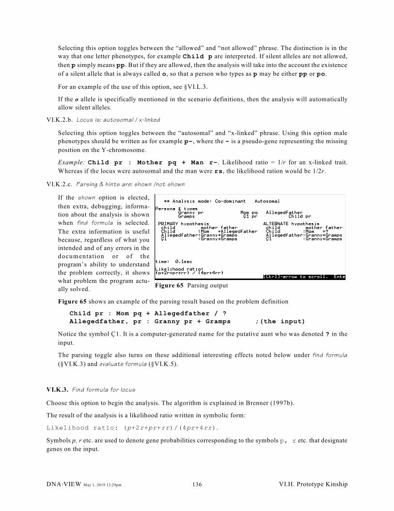
Figure 65 Parsing output
Selecting this option toggles between the “allowed” and “not allowed” phrase. The distinction is in the
way that one letter phenotypes, for example Child p are interpreted. If silent alleles are not allowed,
then p simply means pp. But if they are allowed, then the analysis will take into the account the existence
of a silent allele that is always called o, so that a person who types as p may be either pp or po.
For an example of the use of this option, see §VI.L.3.
If the o allele is specifically mentioned in the scenario definitions, then the analysis will automatically
allow silent alleles.
VI.K.2.b. Locus is: autosomal / x-linked
Selecting this option toggles between the “autosomal” and “x-linked” phrase. Using this option male
phenotypes should be written as for example p–, where the – is a pseudo-gene representing the missing
position on the Y-chromosome.
Example: Child pr : Mother pq + Man r–. Likelihood ratio = 1/r for an x-linked trait.
Whereas if the locus were autosomal and the man were rs, the likelihood ration would be 1/2r.
VI.K.2.c. Parsing & hints are: shown /not shown
If the shown option is elected,
then extra, debugging, informa-
tion about the analysis is shown
when find formula is selected.
The extra information is useful
because, regardless of what you
intended and of any errors in the
docum entation or of the
program’s ability to understand
the problem correctly, it shows
what problem the program actu-
ally solved.
Figure 65 shows an example of the parsing result based on the problem definition
Child pr : Mom pq + Allegedfather / ?Allegedfather, pr : Granny pr + Gramps ;(the input)
Notice the symbol Ç1. It is a computer-generated name for the putative aunt who was denoted ? in the
input.
The parsing toggle also turns on these additional interesting effects noted below under find formula
(§VI.K.3) and evaluate formula (§VI.K.5).
VI.K.3. Find formula for locus
Choose this option to begin the analysis. The algorithm is explained in Brenner (1997b).
The result of the analysis is a likelihood ratio written in symbolic form:
Likelihood ratio: (p+2r+pr+rr)/(4pr+4rr).
Symbols p, r etc. are used to denote gene probabilities corresponding to the symbols p, r etc. that designate
genes on the input.
DNA@VIEW May 1, 2019 12:29pm VI.H. Prototype Kinship136
VI.K.3.a. Parsing toggle
An odometer-like counter at the bottom of the screen indicates progress as the program derives the for-
mula for the scenarios that you have defined. If the parsing toggle (§VI.K.2.c) is turned on, the display
is enhanced and also includes estimated time to finish.
VI.K.3.b. Interrupt
It is easily possible to define a kinship problem that will run for minutes (not to mention weeks). If you
discover that you have done so accidentally, you may wish to cancel the computation, but without losing
your temporary work which ctrl-break would seem to risk. To cater to this situation, ctrl-break has a
special interpretation during find formula only. It produces the dialogue box:
Really interrupt (y)? Or continue (n)?
Typing y will abort the present computation, but does not quit from Kinship so the present pedi-
gree/locus is not lost. Typing ctrl-break a second time will kill Kinship and return to the main menu.
Typing n of course cancels the interruption and computation resumes.
VI.K.4. Algebraically simplify formula (for amusement only)
The option Algebraic simplify in the Kinship sub-menu is a purely cosmetic operation that attempts to simplify
the algebraic expression for the likelihood ratio. For the example, suppose the likelihood ratio is
(a+b+2ab) / (a+b)
Algebraic simplify will rewrite it as:
1 + 2ab/(a+b).
In some cases you can effect repeated simplifications — or at least rewritings of the formula.
This option is experimental and may not always work perfectly. However, the evaluate formula option always
evaluates the original formula, so does not depend on whether Algebraically simplify formula is correct.
VI.K.5. Evaluate formula
Select the Evaluate formula option in order to evaluate the algebraic expression with numeric gene
probabilities (§VIII.C.13).
Evaluate formula creates a form on the screen in which you can type allele probabilities, and the likelihood
ratio formula is evaluated as you do so. The value is dynamically displayed on the screen. After you have
specified all allele frequencies to your satisfaction, esc or click DONE.
For the example above and locus D3S1358, the result is
Using p=0.113 r=0.223 value = 2.12
If Parsing & hints (§VI.K.2.c) is turned on, then the partial derivatives ML/Mv will be displayed showing
how the likelihood ratio L varies with variation in each variable v. The reason for this hint is to give warning
(by a positive partial derivative) of those special occasions where a generously large probability value is anti-
conservative in the sense of exaggerating the strength of the evidence favoring the principal scenario.
DNA@VIEW May 1, 2019 12:29pm VI.H. Prototype Kinship137
VI.K.6. Display pedigree/locus
— can be used at any time to display all information and calculations for the current locus, such as illustrated
in Figure 65.
VI.K.7. Save the pedigree/locus in a complete case
The pedigree/locus can be stashed to the currently active complete case through the command Post this locus
to the complete case. The posting menu includes the options
VI.K.7.a. Locus (I want to select a new one)
Select this option in order to choose a name, from the DNA·VIEW probe/locus list, under which the
pedigree/locus information is to be saved within the complete case.
VI.K.7.b. Serological test (I will select from PATER list)
Select this option in order to choose a name, from PATER’s list of systems, under which the
pedigree/locus information is to be saved within the complete case.
VI.K.7.c. Arbitrary name (I will type it in)
This option allows typing in a name of your choosing under which to file the present pedigree/locus.
VI.K.7.d. Extant name
Post this locus also presents a menu choice for each of the loci that already exist in the current complete
case. Hence you can use this choice as part of the operation of retrieving a pedigree/locus (see rework,
§VI.J.2.c), modifying it, then putting it back.
VI.K.7.e. no option (backspace enter)
has the effect of escaping from the Post this locus to the complete case submenu without doing
anything.
VI.K.8. Display case summary
— can be used at any time to show a line per locus and overall likelihood ratio for the all loci so far posted
to the complete case, as illustrated in Figure 65.
VI.K.9. Run test cases; check program
This option computes the formulas for a collection of test cases, and compares the answers with the correct
formulas. It is a test that the algebraic formula derivation part of the program has not changed since earlier
versions.
VI.K.10. File or fetch complete case
It is not necessary to file the complete case after each locus, or even to file it at all, but it is certainly safest.
The file or fetch menu is the kinship case library directory. It also contains one option labeled
VI.K.10.a. (a new case)
to create a new complete case entry in the kinship case library.
DNA@VIEW May 1, 2019 12:29pm VI.H. Prototype Kinship138
VI.K.10.a.i.) The programs asks for the name. You may type any name including spaces etc up to about
50 characters. This will be the name that appears in the kinship case library directory.
After typing the name, either enter or tab and the complete case will be added to the directory and
saved.
Use of the tab choice will insert the cumulative likelihood ratio at the end of the name. Thus it will
be visible when you view the library directory.
VI.K.10.b. select a case name
After moving the red selection bar to the desired case, there are three keys normally used to confirm the
selection:
VI.K.10.b.i.) PgUp to confirm the selection to fetch the selected case. It will thus become the new
“current case” and supplant the one you have been working on.
VI.K.10.b.ii.) PgDown to confirm the selection to file the current case under the selected name. After
selecting this choice, you then may rename the case (or re-insert the new likelihood ratio) per
§VI.K.10.a.i above.
VI.K.10.b.iii.) Enter is ok either to file or to fetch. The program will then ask which you want, and
proceed per one of the previous two choices.
Once the case is filed it resides on the hard drive and is safe even if you unplug the computer.
VI.K.11. Calculate additional loci (if any)
Often it will be convenient to model the new locus on the previous one. For example, to continue with the
example data of Figure 64 to do the second locus, VWA, choose Edit pedigree/locus and modify the kinship
file to read:
; Example reconstruction case; locus VWAChild prMom pqAuntie qrGranny rsChild : Mom + Allegedfather / ?Allegedfather, Auntie : Granny + Gramps
Then proceed with step §VI.K.3 etc. The formula for this pedigree/locus will be given as:
Likelihood ratio: (1+r) / (4r)
and the result of step §VI.K.5 is
Using q=0.258 value = 1.22
VI.K.12. Revising a complete case
Sometimes a new complete case is based on an old one. For example, it might be desired to pose a modified
scenario problem — compare the same primary scenario with a different alternative scenario. In such an event
the list of loci, the genotype specifications, and the allele probabilities from the former case may be all or
mostly valid for the new problem, and it will be most convenient to model the new case on the old one, locus
by locus.
The routine described in §VI.J.2 works well in such a case.
DNA@VIEW May 1, 2019 12:29pm VI.H. Prototype Kinship139
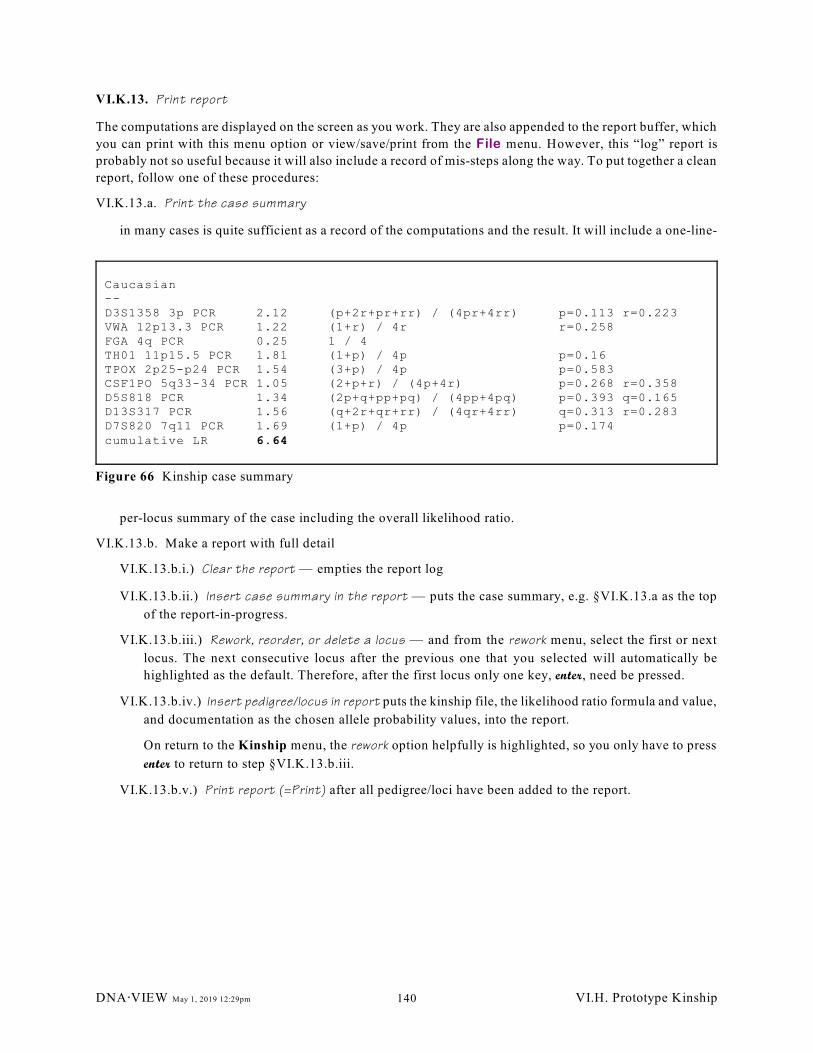
Caucasian--D3S1358 3p PCR 2.12 (p+2r+pr+rr) / (4pr+4rr) p=0.113 r=0.223VWA 12p13.3 PCR 1.22 (1+r) / 4r r=0.258FGA 4q PCR 0.25 1 / 4TH01 11p15.5 PCR 1.81 (1+p) / 4p p=0.16TPOX 2p25-p24 PCR 1.54 (3+p) / 4p p=0.583CSF1PO 5q33-34 PCR 1.05 (2+p+r) / (4p+4r) p=0.268 r=0.358D5S818 PCR 1.34 (2p+q+pp+pq) / (4pp+4pq) p=0.393 q=0.165D13S317 PCR 1.56 (q+2r+qr+rr) / (4qr+4rr) q=0.313 r=0.283D7S820 7q11 PCR 1.69 (1+p) / 4p p=0.174cumulative LR 6.64
Figure 66 Kinship case summary
VI.K.13. Print report
The computations are displayed on the screen as you work. They are also appended to the report buffer, which
you can print with this menu option or view/save/print from the File menu. However, this “log” report is
probably not so useful because it will also include a record of mis-steps along the way. To put together a clean
report, follow one of these procedures:
VI.K.13.a. Print the case summary
in many cases is quite sufficient as a record of the computations and the result. It will include a one-line-
per-locus summary of the case including the overall likelihood ratio.
VI.K.13.b. Make a report with full detail
VI.K.13.b.i.) Clear the report — empties the report log
VI.K.13.b.ii.) Insert case summary in the report — puts the case summary, e.g. §VI.K.13.a as the top
of the report-in-progress.
VI.K.13.b.iii.) Rework, reorder, or delete a locus — and from the rework menu, select the first or next
locus. The next consecutive locus after the previous one that you selected will automatically be
highlighted as the default. Therefore, after the first locus only one key, enter, need be pressed.
VI.K.13.b.iv.) Insert pedigree/locus in report puts the kinship file, the likelihood ratio formula and value,
and documentation as the chosen allele probability values, into the report.
On return to the Kinship menu, the rework option helpfully is highlighted, so you only have to press
enter to return to step §VI.K.13.b.iii.
VI.K.13.b.v.) Print report (=Print) after all pedigree/loci have been added to the report.
DNA@VIEW May 1, 2019 12:29pm VI.H. Prototype Kinship140
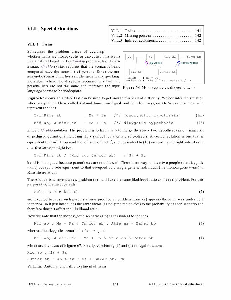
VI.L.1 Twins.. . . . . . . . . . . . . . . . . . . . . . . . . . . . 141
VI.L.2 Missing persons.. . . . . . . . . . . . . . . . . . . . 142
VI.L.3 Indirect exclusions.. . . . . . . . . . . . . . . . . . 142
Figure 68 Monozygotic vs. dizygotic twins
VI.L. Special situations
VI.L.1. Twins
Sometimes the problem arises of deciding
whether twins are monozygotic or dizygotic. This seems
like a natural target for the Kinship program, but there is
a snag: Kinship syntax requires that the scenarios being
compared have the same list of persona. Since the mo-
nozygotic scenario implies a single (genetically speaking)
individual where the dizygotic scenario has two, the
persona lists are not the same and therefore the input
language seems to be inadequate.
Figure 67 shows an artifice that can be used to get around this kind of difficulty. We consider the situation
where only the children, called Kid and Junior, are typed, and both heterozygous ab. We need somehow to
represent the idea
TwinKids ab : Ma + Pa /*/ monozygotic hypothesis (1m)
Kid ab, Junior ab : Ma + Pa /*/ dizygotic hypothesis (1d)
in legal Kinship notation. The problem is to find a way to merge the above two hypotheses into a single set
of pedigree definitions including the / symbol for alternate role-players. A correct solution is one that is
equivalent to (1m) if you read the left side of each /, and equivalent to (1d) on reading the right side of each
/. A first attempt might be:
TwinKids ab / (Kid ab, Junior ab) : Ma + Pa
but this is no good because parentheses are not allowed. There is no way to have two people (the dizygotic
twins) occupy a role equivalent to that occupied by a single genetic individual (the monozygotic twins) in
Kinship notation.
The solution is to invent a new problem that will have the same likelihood ratio as the real problem. For this
purpose two mythical parents
Able aa % Baker bb (2)
are invented because such parents always produce ab children. Line (2) appears the same way under both
scenarios, so it just introduces the same factor (namely the factor a b ) to the probability of each scenario and2 2
therefore doesn’t affect the likelihood ratio.
Now we note that the monozygotic scenario (1m) is equivalent to the idea
Kid ab : Ma + Pa % Junior ab : Able aa + Baker bb (3)
whereas the dizygotic scenario is of course just:
Kid ab, Junior ab : Ma + Pa % Able aa % Baker bb (4)
which are the ideas of Figure 67. Finally, combining (3) and (4) in legal notation:
Kid ab : Ma + Pa
Junior ab : Able aa / Ma + Baker bb/ Pa
VI.L.1.a. Automatic Kinship treatment of twins
DNA@VIEW May 1, 2019 12:29pm VI.L. Kinship – special situations141
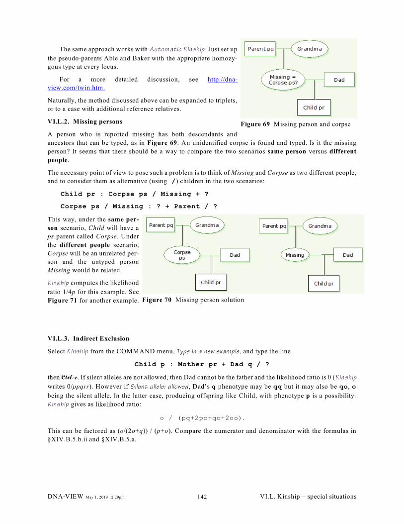
Figure 69 Missing person and corpse
Figure 70 Missing person solution
The same approach works with Automatic Kinship. Just set up
the pseudo-parents Able and Baker with the appropriate homozy-
gous type at every locus.
For a more detailed discussion, see http://dna-
view.com/twin.htm.
Naturally, the method discussed above can be expanded to triplets,
or to a case with additional reference relatives.
VI.L.2. Missing persons
A person who is reported missing has both descendants and
ancestors that can be typed, as in Figure 69. An unidentified corpse is found and typed. Is it the missing
person? It seems that there should be a way to compare the two scenarios same person versus different
people.
The necessary point of view to pose such a problem is to think of Missing and Corpse as two different people,
and to consider them as alternative (using /) children in the two scenarios:
Child pr : Corpse ps / Missing + ?
Corpse ps / Missing : ? + Parent / ?
This way, under the same per-
son scenario, Child will have a
ps parent called Corpse. Under
the different people scenario,
Corpse will be an unrelated per-
son and the untyped person
Missing would be related.
Kinship computes the likelihood
ratio 1/4p for this example. See
Figure 71 for another example.
VI.L.3. Indirect Exclusion
Select Kinship from the COMMAND menu, Type in a new example, and type the line
Child p : Mother pr + Dad q / ?
then Ctrl-e. If silent alleles are not allowed, then Dad cannot be the father and the likelihood ratio is 0 (Kinship
writes 0/ppqrr). However if Silent allele: allowed, Dad’s q phenotype may be qq but it may also be qo, o
being the silent allele. In the latter case, producing offspring like Child, with phenotype p is a possibility.
Kinship gives as likelihood ratio:
o / (pq+2po+qo+2oo).
This can be factored as (o/(2o+q)) / (p+o). Compare the numerator and denominator with the formulas in
§XIV.B.5.b.ii and §XIV.B.5.a.
DNA@VIEW May 1, 2019 12:29pm VI.L. Kinship – special situations142
VII. DISASTER ANALYSIS
VII.A. Overview
The DNA·VIEW disaster analysis module is designed to identify victims with references by DNA types.
Victims are an arbitrary list of DNA profiles. References are another arbitrary list, but also, to the extent that
the reference list includes several samples that belong to the same case, they are treated as a family. Multiple
family members who seem to resemble the same victim are especially noted in the screening. The present
version takes no particular systematic account of possible genetic relationships among victims, although the
Kinship module of course permits assessment of all potential relationships.
Some of the programs are customized specifically for World Trade Center (WTC) identification data formats,
and parts of this documentation reflect this. The modules are, however, ready to be used for any disaster.
The principal actions for victim identification are grouped in the Disaster Screening menu.
VII.A.1. There are four major steps to the analysis:
VII.B Import DNA profiles.. . . . . . . . . . . . . . . . . . . . . . . . . . . . . . . . . . . . . . . . . . . . . . . . . . page 144
The input file can have all profiles – family reference, personal reference, and victim – mixed
together.
Time: Importing 15,000 samples takes a few minutes.
VII.C Collapse victim reference list. . . . . . . . . . . . . . . . . . . . . . . . . . . . . . . . . . . . . . . . . . . . page 145
Reduce the victim list by removing duplicates and probable duplicates
VII.D Screen for candidate family-victim matches. . . . . . . . . . . . . . . . . . . . . . . . . . . . . . . . . page 148
The screen computes likelihood ratios for identity, parent/child (accounting for mutation), and sibship
between every family member and every victim profile. More importantly, it tests for two different
family members resembling the same victim.
The resultant list is sorted by family in order of promise.
Time: 20 minutes to screen 2600 families (3+ members each) against 2000 (distinct) victims.
VII.F Test the matches with an accurate computation. . . . . . . . . . . . . . . . . . . . . . . . . . . . . . page 153
Compute a likelihood ratio for any combination of people.
Time: 1 minute - 1 hour per family, depending on success and complexity.
DNA@VIEW May 1, 2019 12:29pm VII. Disaster screening143
VII.A.2. Additional – method+tool to establish reference allele frequencies
VII.G Assign race to worklist. . . . . . . . . . . . . . . . . . . . . . . . . . . . . . . . . . . . . . . . . . . . . . . . page 156
preparatory to compiling disaster-specific population frequencies.
VII.B. Import DNA profiles
VII.B.1. Overview
VII.B.1.a. Lists
The object of importing is to create lists – worklists of profiles to compare against one another. Typically
create these lists:
VII.B.1.a.i.) Family+Personal references
The reference for each victim should be grouped together in a case, meaning that you assign a case
number corresponding to each missing person.
Grouping them makes it possible for the screening heuristic to make better judgements than if it
could only compare one-to-one.
VII.B.1.a.ii.) role letters for references
Putting the references into cases means assigning them role letters.
» For relatives of a missing person the role letter assignment under “Kinship roles” in Figure 154
are suggestions.
» Eventually, when a likely candidate for the victim is recognized, that victim profile will also
(tentatively) be added to the case, normally with a role letter of V or W.
» For personal references – DNA profiles or partial profiles that represent the missing person such
as a profile obtained from a toothbrush or neonatal heel prick – the letters J, K, and L are
preferred, especially if there are multiple personal reference profiles in the case. Those letters are
treated in a slightly special way by the screening heuristic in that it recognizes they are probably
versions of the same profile.
VII.B.1.a.iii.) Victim profile
The victim profile list is a set of profiles which have accession numbers but are normally not part of
any case, at least not initially.
The screening program is arranged so that each list may be in several parts, i.e. may consists of several
worklists.
VII.B.1.b. Repetitive screening
During the course of analysis of a mass disaster, new DNA profiles are likely to be developed continually
over a considerable time. Screening and identification will go along in parallel. Therefore it will be
desired to run the screening process repetitively. This can be done either
VII.B.1.b.i.) incrementally – by adding new data to the old in DNAAVIEW, possibly by adding additional
worklists
VII.B.1.b.ii.) by starting over each time, re-installing DNAAVIEW with empty data files, then importing
all accumulated data.
DNA@VIEW May 1, 2019 12:29pm VII. Disaster screening144
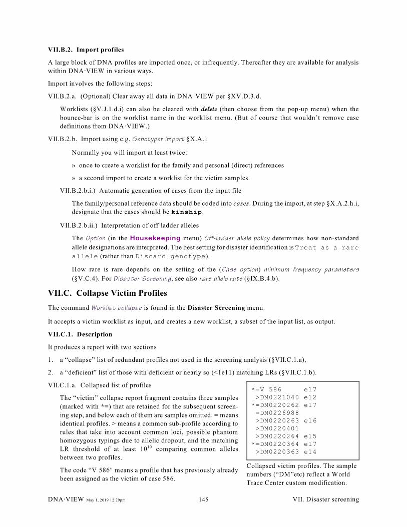
*=V 586 e17 >DM0221040 e12 *=DM0220262 e17 =DM0226988 >DM0220263 e16 >DM0220401 >DM0220264 e15 *=DM0220364 e17 >DM0220363 e14
Collapsed victim profiles. The sample
numbers (“DM”etc) reflect a World
Trace Center custom modification.
VII.B.2. Import profiles
A large block of DNA profiles are imported once, or infrequently. Thereafter they are available for analysis
within DNA@VIEW in various ways.
Import involves the following steps:
VII.B.2.a. (Optional) Clear away all data in DNA·VIEW per §XV.D.3.d.
Worklists (§V.J.1.d.i) can also be cleared with delete (then choose from the pop-up menu) when the
bounce-bar is on the worklist name in the worklist menu. (But of course that wouldn’t remove case
definitions from DNA·VIEW.)
VII.B.2.b. Import using e.g. Genotyper Import §X.A.1
Normally you will import at least twice:
» once to create a worklist for the family and personal (direct) references
» a second import to create a worklist for the victim samples.
VII.B.2.b.i.) Automatic generation of cases from the input file
The family/personal reference data should be coded into cases. During the import, at step §X.A.2.h.i,
designate that the cases should be kinship.
VII.B.2.b.ii.) Interpretation of off-ladder alleles
The Option (in the Housekeeping menu) Off-ladder allele policy determines how non-standard
allele designations are interpreted. The best setting for disaster identification is Treat as a rare
allele (rather than Discard genotype).
How rare is rare depends on the setting of the (Case option) minimum frequency parameters
(§V.C.4). For Disaster Screening, see also rare allele rate (§IX.B.4.b).
VII.C. Collapse Victim Profiles
The command Worklist collapse is found in the Disaster Screening menu.
It accepts a victim worklist as input, and creates a new worklist, a subset of the input list, as output.
VII.C.1. Description
It produces a report with two sections
1. a “collapse” list of redundant profiles not used in the screening analysis (§VII.C.1.a),
2. a “deficient” list of those with deficient or nearly so (<1e11) matching LRs (§VII.C.1.b).
VII.C.1.a. Collapsed list of profiles
The “victim” collapse report fragment contains three samples
(marked with *=) that are retained for the subsequent screen-
ing step, and below each of them are samples omitted. = means
identical profiles. > means a common sub-profile according to
rules that take into account common loci, possible phantom
homozygous typings due to allelic dropout, and the matching
LR threshold of at least 10 comparing common alleles10
between two profiles.
The code “V 586" means a profile that has previously already
been assigned as the victim of case 586.
DNA@VIEW May 1, 2019 12:29pm VII. Disaster screening145
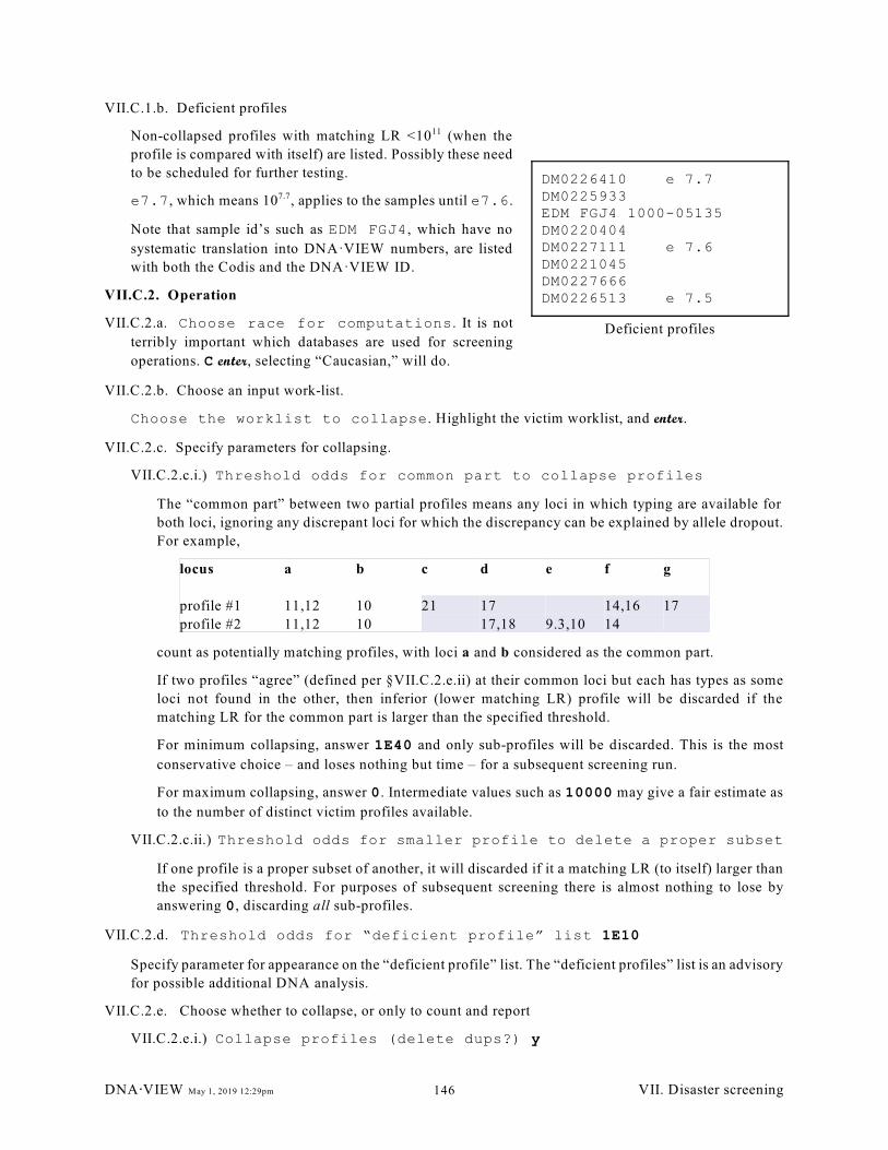
DM0226410 e 7.7DM0225933 EDM FGJ4 1000-05135 DM0220404 DM0227111 e 7.6DM0221045 DM0227666 DM0226513 e 7.5
Deficient profiles
VII.C.1.b. Deficient profiles
Non-collapsed profiles with matching LR <10 (when the11
profile is compared with itself) are listed. Possibly these need
to be scheduled for further testing.
e7.7, which means 10 , applies to the samples until e7.6.7.7
Note that sample id’s such as EDM FGJ4, which have no
systematic translation into DNA·VIEW numbers, are listed
with both the Codis and the DNA·VIEW ID.
VII.C.2. Operation
VII.C.2.a. Choose race for computations. It is not
terribly important which databases are used for screening
operations. C enter, selecting “Caucasian,” will do.
VII.C.2.b. Choose an input work-list.
Choose the worklist to collapse. Highlight the victim worklist, and enter.
VII.C.2.c. Specify parameters for collapsing.
VII.C.2.c.i.) Threshold odds for common part to collapse profiles
The “common part” between two partial profiles means any loci in which typing are available for
both loci, ignoring any discrepant loci for which the discrepancy can be explained by allele dropout.
For example,
locus a b c d e f g
profile #1 11,12 10 21 17 14,16 17
profile #2 11,12 10 17,18 9.3,10 14
count as potentially matching profiles, with loci a and b considered as the common part.
If two profiles “agree” (defined per §VII.C.2.e.ii) at their common loci but each has types as some
loci not found in the other, then inferior (lower matching LR) profile will be discarded if the
matching LR for the common part is larger than the specified threshold.
For minimum collapsing, answer 1E40 and only sub-profiles will be discarded. This is the most
conservative choice – and loses nothing but time – for a subsequent screening run.
For maximum collapsing, answer 0. Intermediate values such as 10000 may give a fair estimate as
to the number of distinct victim profiles available.
VII.C.2.c.ii.) Threshold odds for smaller profile to delete a proper subset
If one profile is a proper subset of another, it will discarded if it a matching LR (to itself) larger than
the specified threshold. For purposes of subsequent screening there is almost nothing to lose by
answering 0, discarding all sub-profiles.
VII.C.2.d. Threshold odds for “deficient profile” list 1E10
Specify parameter for appearance on the “deficient profile” list. The “deficient profiles” list is an advisory
for possible additional DNA analysis.
VII.C.2.e. Choose whether to collapse, or only to count and report
VII.C.2.e.i.) Collapse profiles (delete dups?) y
DNA@VIEW May 1, 2019 12:29pm VII. Disaster screening146
VII.C.2.e.ii.) Exact, Lenient, or Dropout, or STR dropout collapsing? D
Dropout means 12 matches 12,13 or 13, but not 14,15. It is permissive of allelic dropout and seems
realistic for degraded STR samples.
L STR dropout (recommended) uses the Dropout rule for STR’s but requires an exact match for
SNP’s. This is a bit conservative for SNP’s but there is no harm except computation time for
retaining some unnecessary SNP profiles.
Exact matching means 12 doesn't match 12,13. Allelic dropout is considered impossible.
Lenient means 12 matches 12,13 or 13 or even 14,15. (This unrealistic choice was originally
implemented as an approximation to the more complicated “dropout” option.)
VII.C.2.e.iii.) Choose a worklist for saving the collapsed list
Either create a new empty worklist, or select a scratch worklist that you are using for this purpose.
The output of Worklist Collapse will be the input for a subsequent Screen disaster matches
(§VII.D).
DNA@VIEW May 1, 2019 12:29pm VII. Disaster screening147
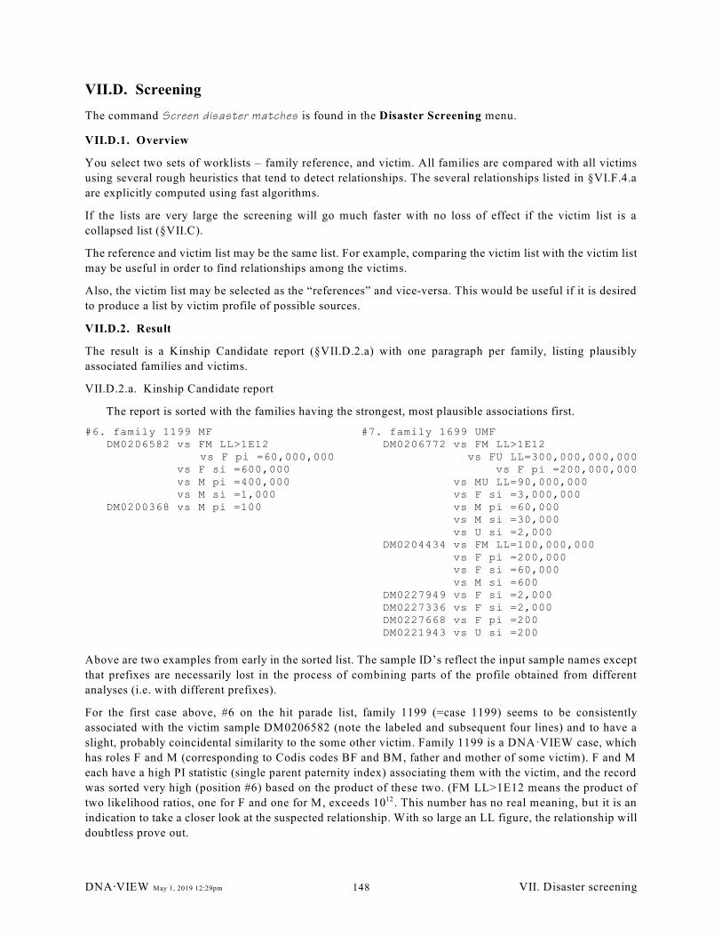
VII.D. Screening
The command Screen disaster matches is found in the Disaster Screening menu.
VII.D.1. Overview
You select two sets of worklists – family reference, and victim. All families are compared with all victims
using several rough heuristics that tend to detect relationships. The several relationships listed in §VI.F.4.a
are explicitly computed using fast algorithms.
If the lists are very large the screening will go much faster with no loss of effect if the victim list is a
collapsed list (§VII.C).
The reference and victim list may be the same list. For example, comparing the victim list with the victim list
may be useful in order to find relationships among the victims.
Also, the victim list may be selected as the “references” and vice-versa. This would be useful if it is desired
to produce a list by victim profile of possible sources.
VII.D.2. Result
The result is a Kinship Candidate report (§VII.D.2.a) with one paragraph per family, listing plausibly
associated families and victims.
VII.D.2.a. Kinship Candidate report
The report is sorted with the families having the strongest, most plausible associations first.
#6. family 1199 MF DM0206582 vs FM LL>1E12 vs F pi =60,000,000 vs F si =600,000 vs M pi =400,000 vs M si =1,000 DM0200368 vs M pi =100
#7. family 1699 UMF DM0206772 vs FM LL>1E12 vs FU LL=300,000,000,000 vs F pi =200,000,000 vs MU LL=90,000,000 vs F si =3,000,000 vs M pi =60,000 vs M si =30,000 vs U si =2,000 DM0204434 vs FM LL=100,000,000 vs F pi =200,000 vs F si =60,000 vs M si =600 DM0227949 vs F si =2,000 DM0227336 vs F si =2,000 DM0227668 vs F pi =200 DM0221943 vs U si =200
Above are two examples from early in the sorted list. The sample ID’s reflect the input sample names except
that prefixes are necessarily lost in the process of combining parts of the profile obtained from different
analyses (i.e. with different prefixes).
For the first case above, #6 on the hit parade list, family 1199 (=case 1199) seems to be consistently
associated with the victim sample DM0206582 (note the labeled and subsequent four lines) and to have a
slight, probably coincidental similarity to the some other victim. Family 1199 is a DNA·VIEW case, which
has roles F and M (corresponding to Codis codes BF and BM, father and mother of some victim). F and M
each have a high PI statistic (single parent paternity index) associating them with the victim, and the record
was sorted very high (position #6) based on the product of these two. (FM LL>1E12 means the product of
two likelihood ratios, one for F and one for M, exceeds 10 . This number has no real meaning, but it is an12
indication to take a closer look at the suspected relationship. With so large an LL figure, the relationship will
doubtless prove out.
DNA@VIEW May 1, 2019 12:29pm VII. Disaster screening148
The second case shows that family 1699 may well be full sibling (U) mother (M), and father (F) to
DM0206772. The line vs U si=2,000 means that U and the victim have a similarity that is characteristic
of siblings (si=sibling index, that is, likelihood ratio favoring full-siblingship over unrelatedness).
The product of two likelihoods for DM0204434 is also so high (100,000,000), that probably these two
samples represent the same person. The situation of two strong candidates, as here, is rare because the
collapsing algorithm (§VII.C) will usually eliminate a redundant profile (the probable situation here).
VII.D.2.b. Screening
Then, the family-by-family analysis proceeds, comparing the families one at a time with all victims and
preparing a paragraph per family as shown above. The screening step is very fast – typically several
families per second although slower if there are thousands of victims or profiles have many loci.
You may interrupt the screening, for amusement, by hitting any key. Then you can space to step forward
one family at a time, or r when bored to allow the program to resume at full speed. The program also
responds to the b (back up) instruction, however beware: If you back up to a family for which the
analysis just added a victim candidate, the second analysis of that family will regard the victim as
previously, not newly, entered. This may affect the sorting of the final report.
The family paragraphs are then sorted according to a rough measure of likelihood of including a correct
association, and compiled into a report. The report is again presented for cursory inspection (see §V.K.3).
Hit esc when done cursorily inspecting. Then, from the main menu, you may print or file it as described
above.
The families and associated victims may be regarded as kinship candidates.
VII.D.3. Operation
VII.D.3.a. Choose one or several races for searching computations. The best strategy is to nominate all the
major races likely to be relevant. Enter the set of races with a string of one-letter abbreviations (per
Codings for races, §IX.A.4)
See §IX.B.3.f for some details of Screen allele probabilities.
VII.D.3.b. Choose two sets of worklists to screen against one another (which need not be different)
Choose the worklist with the families. Highlight a family worklist, and enter.
Any more worklists besides those below? is offered repeatedly to allow several
worklists to be combined in case the references are not all on one worklist.
Choose the worklist with the victims. Highlight the victim worklist, and enter.
Any more worklists besides those below? is offered repeatedly to allow several
worklists to be combined in case the victims are not all on one worklist.
VII.D.3.c. Select the screening heuristic rules and parameters
VII.D.3.c.i.) Family parameters/rules – if the reference list includes family groups (i.e. cases)
Sort screening candidates (most promising first)? yes
Normally y seems the more useful result. However, if screening victims against victims and the
aim is to have a directory that can be manually searched by victim, the unsorted report would be
easier to use.
but sort families last if comment includes '>>'? yes
To take advantage of this option, manually insert the character pair >> at any point in the case
comment (§V.B.11; see also §V.B.28.a.ii) for any identification case that is complete or nearly
DNA@VIEW May 1, 2019 12:29pm VII. Disaster screening149
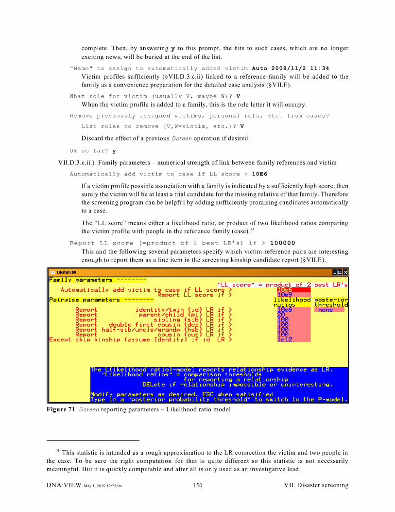
Figure 71 Screen reporting parameters – Likelihood ratio model
complete. Then, by answering y to this prompt, the hits to such cases, which are no longer
exciting news, will be buried at the end of the list.
"Name" to assign to automatically added victim Auto 2008/11/2 11:34
Victim profiles sufficiently (§VII.D.3.c.ii) linked to a reference family will be added to the
family as a convenience preparation for the detailed case analysis (§VII.F).
What role for victim (usually V, maybe W)? V
When the victim profile is added to a family, this is the role letter it will occupy.
Remove previously assigned victims, personal refs, etc. from cases?
List roles to remove (V,W=victim, etc.)? V
Discard the effect of a previous Screen operation if desired.
Ok so far? y
VII.D.3.c.ii.) Family parameters – numerical strength of link between family references and victim
Automatically add victim to case if LL score > 10E6
If a victim profile possible association with a family is indicated by a sufficiently high score, then
surely the victim will be at least a trial candidate for the missing relative of that family. Therefore
the screening program can be helpful by adding sufficiently promising candidates automatically
to a case.
The “LL score” means either a likelihood ratio, or product of two likelihood ratios comparing
the victim profile with people in the reference family (case).14
Report LL score (=product of 2 best LR's) if > 100000
This and the following several parameters specify which victim-reference pairs are interesting
enough to report them as a line item in the screening kinship candidate report (§VII.E).
This statistic is intended as a rough approximation to the LR connection the victim and two people in14
the case. To be sure the right computation for that is quite different so this statistic is not necessarily
meaningful. But it is quickly computable and after all is only used as an investigative lead.
DNA@VIEW May 1, 2019 12:29pm VII. Disaster screening150
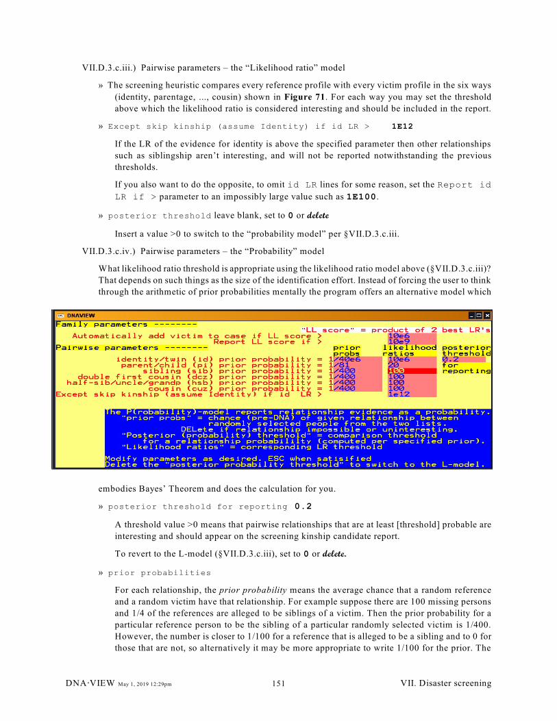
VII.D.3.c.iii.) Pairwise parameters – the “Likelihood ratio” model
» The screening heuristic compares every reference profile with every victim profile in the six ways
(identity, parentage, ..., cousin) shown in Figure 71. For each way you may set the threshold
above which the likelihood ratio is considered interesting and should be included in the report.
» Except skip kinship (assume Identity) if id LR > 1E12
If the LR of the evidence for identity is above the specified parameter then other relationships
such as siblingship aren’t interesting, and will not be reported notwithstanding the previous
thresholds.
If you also want to do the opposite, to omit id LR lines for some reason, set the Report id
LR if > parameter to an impossibly large value such as 1E100.
» posterior threshold leave blank, set to 0 or delete
Insert a value >0 to switch to the “probability model” per §VII.D.3.c.iii.
VII.D.3.c.iv.) Pairwise parameters – the “Probability” model
What likelihood ratio threshold is appropriate using the likelihood ratio model above (§VII.D.3.c.iii)?
That depends on such things as the size of the identification effort. Instead of forcing the user to think
through the arithmetic of prior probabilities mentally the program offers an alternative model which
embodies Bayes’ Theorem and does the calculation for you.
» posterior threshold for reporting 0.2
A threshold value >0 means that pairwise relationships that are at least [threshold] probable are
interesting and should appear on the screening kinship candidate report.
To revert to the L-model (§VII.D.3.c.iii), set to 0 or delete.
» prior probabilities
For each relationship, the prior probability means the average chance that a random reference
and a random victim have that relationship. For example suppose there are 100 missing persons
and 1/4 of the references are alleged to be siblings of a victim. Then the prior probability for a
particular reference person to be the sibling of a particular randomly selected victim is 1/400.
However, the number is closer to 1/100 for a reference that is alleged to be a sibling and to 0 for
those that are not, so alternatively it may be more appropriate to write 1/100 for the prior. The
DNA@VIEW May 1, 2019 12:29pm VII. Disaster screening151
only risk is that somewhat more non-siblings who coincidentally look like siblings will clutter
up the screening report.
VII.E. Screening summary
Anytime after running a Screen, you may run this command to prepare a brief report based on the Screen run.
The result is a 5-column, tab-delimited file that you can import to Excel to view, sort, and manipulate.
The file contains one row for each plausible connection between a sample from the victim worklists ("bone")
and a reference family from the reference worklists, per §VII.D.3.b. "Plausible connection" is defined by the
value chosen for the last of the screening analysis parameters of, Report LL score (§VII.D.3.c.ii).
The columns within each row are:
RM# a case number
bone the accession number of a bone possibly related to the references of the case.
Role of bone In case the bone already is part of a case
Case of bone In case the bone already is part of a case
LL score The qualifying score; product of the two largest relationship scores between
the bone and two different references in the case.
DNA@VIEW May 1, 2019 12:29pm VII. Disaster screening152
VII.F. Test Candidate Relationship using Kinship
Start from the top of the family screening hit parade, and one at a time test the families with their likely
associated victims using the Automatic Kinship Case program. Assuming the expected result with a
satisfactory likelihood ratio is obtained, the victim can be regarded as identified.
VII.F.1. Kinship steps
From the command menu, choose Casework < Automatic Kinship < select case.
VII.F.1.a. Case #
Type in a case number, e.g. 1199 enter to work the first case shown in §VII.D.2.a.
VII.F.1.b. Insert, if necessary, the suspected associated victim
If the case has no victim already, Add role should be highlighted. Enter to select it.
Victim should be highlighted. Enter to select it.
Type 0200 space 06582 end to add DM0206582 as role V of the case. (Actually leading 0's can be
elided.)
VII.F.1.c. Go to kinship and evaluate
Strike / to highlight Immigration/Kinship. Enter to select it.
Test the relationships using the methods detailed in the DNA·VIEW manual. Chapter VI, Kinship, covers
the principles of kinship scenario specification and analysis, and details of using the program. In outline:
VII.F.1.c.i.) Type in scenario 1
VII.F.1.c.ii.) Shortcut to analyze all races
Calculate & report LRs, [all] races determines the formulas, evaluates them for all races in the race
list, and displays and adds to the report summary box with the bottom line for each race.
The more detailed per-race, per-locus calculation summaries are available if desired, or the report can
be kept very brief:
Include per/locus details for each race in report? n
VII.F.1.c.iii.) Exit from kinship
Note that after some kinship operations a result will be displayed and a yellow wait banner will be
at the bottom of the screen. It is not necessary to type enter, then q to advance to the kinship menu
and select quit from immigration; you can save a keystroke by typing q at the wait.
VII.F.2. Technical comments about evaluating identifications
Alternates to the victim
VII.F.2.a.i.) Simple examples
Suppose the victim is denoted V and the suspected relationship is V:M+F. The alternative relationship
can be thought of either as V:?+? (recall that each ? asks the program to substitute a new unique
name), or as ?:M+F. The second version leads to the more attractive combined formula: V/?:M+F
expressing the scenarios to be contrasted.
DNA@VIEW May 1, 2019 12:29pm VII. Disaster screening153
Similarly, if the suspected relationship is S,D:?+V, the combined formula can be written as
S,D:?+V/?.
VII.F.2.a.ii.) Mistake to avoid
From the foregoing examples, it is tempting to conclude that the combined formula can always be
obtained from the suspected relationship by noting each instance of V and substituting V/?. Not true.
It is safe, however, to substitute always V/Other.
The problem occurs when V needs to be mentioned twice. For example, suppose that the suspected
relationships are
V : M + FS : Spouse + V
Then the alternate relationships are not defined by the formulation
? : M + FS : Spouse + ?
because each separate instance of ? by definition refers to a different person, so it does not include
the information that S is related to M and to F. Therefore the combined form
V/? : M + FS : Spouse + V/?
is incorrect. It biases the computation towards the suspected relationships. Correct is
V/Other : M + FS : Spouse + V/Other
VII.F.2.b. Likelihood ratio from Amelogenin
Almost all the victims (>80%) are male. Therefore a likelihood ratio of 2,000,000 from autosomal loci
for identifying a male victim is not augmented very much by the evidential value of having the expected
Amelogenin type.
VII.F.3. More hints
VII.F.3.a. Pick list
The “pick list” can be useful. There are no doubt many cases with a reference mother, child, and sibling:
Therefore it might be convenient to can the formula
V/Other:M + FU : M + F
by adding it to the pick list.
Note that this same formulation is perfectly correct if the mother is not typed – there is no reason not to
call her M anyway. Also, even if there is no sibling reference U, nothing is lost by including the second
line except a barely perceptible amount of computation time.
VII.F.3.b. Mutations
The toggle Do (don’t) consider mutation means that the likelihood ratio will never be reported as zero,
but instead a small number will be reported. See §XIII.C.4, page284.
The small number is a reasonable estimate of the rate of paternal one-step mutations for the locus, but
it is by no means therefore a reasonable estimate of the likelihood ratio for the present problem.
DNA@VIEW May 1, 2019 12:29pm VII. Disaster screening154
Example: Suppose a possible victim is being compared to two parent referenced: V/Other:M+F and
in some locus the putative victim is PQ, the mother is PP, and the man is Q R, where Q is one step+ +
(repeat number) larger than Q.
Let p, q, ì be the probabilities of P and Q, and the mutation rate for the locus. Assuming, then, that half
of all mutations are by minus one step,
Pr(genetic data | right victim) = Pr(PP woman)·Pr(Q R man)· ½ ·½ ì and+
Pr(genetic data | wrong victim) = Pr(PP woman)·Pr(Q R man)·2pq, +
so the likelihood ratio is ì/8pq, which may be much larger than ì although typically it is about 3ì.
In general, the mutation computation from the program should be regarded as no more than a signal.
Mutations need to be worked out by hand.
VII.F.3.c. Allelic dropout
Assuming the same scenario as in the previous section, suppose the victim is P, the mother is P, and the
father is QR. The program will of course report a mutation result, but in this case the real explanation
may be not mutation but allelic dropout: the victim is really PQ.
A different, but still manual, analysis is necessary if this possibility is to be taken into account.
VII.F.3.c.i.) fudge the data
Examination of electropherograms may reveal a plausible Q in the victim. If so, modify (change and
re-import the data file or use Type in a Read, §IV.D.4) the victim profile. Run the kinship analysis
again. The formula will be 1/4pq.
VII.F.3.c.ii.) Possible dropout
Alternatively, suppose dropout is reckoned to be a possibility, but not a certainty. Then we need to
use some estimate for the chance of dropout, the probability
z = Pr( not see Q allele | Q allele exists)
Assuming z is known, then
Pr(genetic data | right victim) = Pr(PP woman)·Pr(QR man)· ½ ·z and
Pr(genetic data | wrong victim) = Pr(PP woman)·Pr(QR man)·[2pqz + pp].
The right likelihood ratio is therefore z/[4pqz+2pp], which is roughly z times the result obtained
above by assuming that dropout definitely occurred.
VII.F.3.c.iii.) Summary
A reasonable rough estimate of the likelihood ratio for a locus with possible dropout is obtained by
modifying the data to the suspected (non-dropout) types, running the Kinship analysis, and
multiplying the result by z.
DNA@VIEW May 1, 2019 12:29pm VII. Disaster screening155
VII.G. Assign Race to Worklist
In assessing a possible relationship between a victim and a reference sample, the relevant probability is the
relative likelihood that some unrelated victim sample would bear the observed resemblance with the
reference. Therefore the relevant population sample to consider is the victims.
To create a set of victim allele frequency databases,
VII.G.1.a.i.) Import victim profiles to a worklist, per §VII.B.
VII.G.1.a.ii.) Use Assign race to worklist (in the Disaster analysis menu) to assign an otherwise
unused race letter – e.g. w – to every sample in the victim worklist(s).
Equally, when viewing the list of worklists (e.g. using Worklist, §V.J), put the red bar on the desired
worklist and click the ASSIGN RACE button.
You can optionally exclude assigning any race to children, which is usually a good option.
VII.G.1.a.iii.) Create databases, one for each locus, for the victim race. The protocol for doing this is
detailed in §VIII.C.4 Building and maintaining allele population data (“database”) in DNA@VIEW.
DNA@VIEW May 1, 2019 12:29pm VII. Disaster screening156
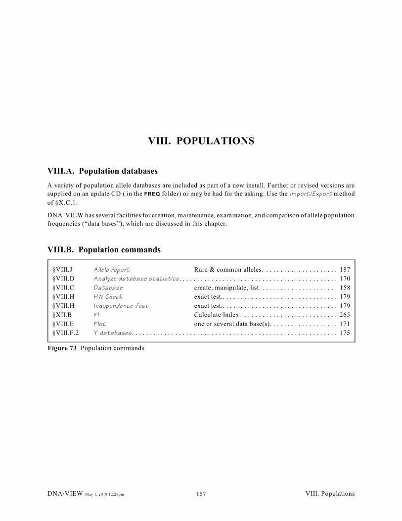
§VIII.J Allele report Rare & common alleles. . . . . . . . . . . . . . . . . . . . . 187
§VIII.D Analyze database statistics . . . . . . . . . . . . . . . . . . . . . . . . . . . . . . . . . . . . . . . . . . . . 170
§VIII.C Database create, manipulate, list. . . . . . . . . . . . . . . . . . . . . . 158
§VIII.H HW Check exact test.. . . . . . . . . . . . . . . . . . . . . . . . . . . . . . . . 179
§VIII.H Independence Test exact test.. . . . . . . . . . . . . . . . . . . . . . . . . . . . . . . . 179
§XII.B PI Calculate Index. . . . . . . . . . . . . . . . . . . . . . . . . . . 265
§VIII.E Plot one or several data base(s). . . . . . . . . . . . . . . . . . . 171
§VIII.F.2 Y databases. . . . . . . . . . . . . . . . . . . . . . . . . . . . . . . . . . . . . . . . . . . . . . . . . . . . . . . . . 175
Figure 73 Population commands
VIII. POPULATIONS
VIII.A. Population databases
A variety of population allele databases are included as part of a new install. Further or revised versions are
supplied on an update CD ( in the FREQ folder) or may be had for the asking. Use the Import/Export method
of §X.C.1.
DNA·VIEW has several facilities for creation, maintenance, examination, and comparison of allele population
frequencies (“data bases”), which are discussed in this chapter.
VIII.B. Population commands
DNA@VIEW May 1, 2019 12:29pm VIII. Populations157
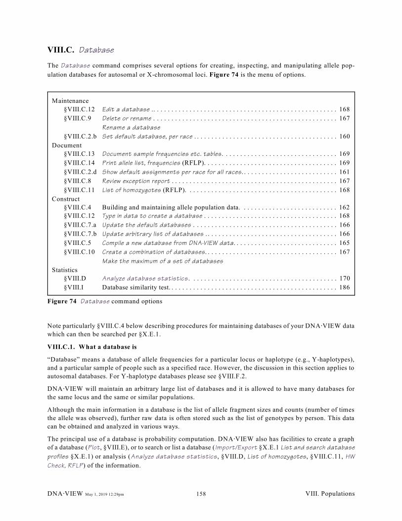
Maintenance
§VIII.C.12 Edit a database .. . . . . . . . . . . . . . . . . . . . . . . . . . . . . . . . . . . . . . . . . . . . . . . . . . . 168
§VIII.C.9 Delete or rename . . . . . . . . . . . . . . . . . . . . . . . . . . . . . . . . . . . . . . . . . . . . . . . . . . . 167
Rename a database
§VIII.C.2.b Set default database, per race . . . . . . . . . . . . . . . . . . . . . . . . . . . . . . . . . . . . . . . . 160
Document
§VIII.C.13 Document sample frequencies etc. tables. . . . . . . . . . . . . . . . . . . . . . . . . . . . . . . . 169
§VIII.C.14 Print allele list, frequencies (RFLP). . . . . . . . . . . . . . . . . . . . . . . . . . . . . . . . . . . . . 169
§VIII.C.2.d Show default assignments per race for all races. . . . . . . . . . . . . . . . . . . . . . . . . . . 161
§VIII.C.8 Review exception report . . . . . . . . . . . . . . . . . . . . . . . . . . . . . . . . . . . . . . . . . . . . . . 167
§VIII.C.11 List of homozygotes (RFLP). . . . . . . . . . . . . . . . . . . . . . . . . . . . . . . . . . . . . . . . . . 168
Construct
§VIII.C.4 Building and maintaining allele population data. . . . . . . . . . . . . . . . . . . . . . . . . . . 162
§VIII.C.12 Type in data to create a database . . . . . . . . . . . . . . . . . . . . . . . . . . . . . . . . . . . . . 168
§VIII.C.7.a Update the default databases . . . . . . . . . . . . . . . . . . . . . . . . . . . . . . . . . . . . . . . . 166
§VIII.C.7.b Update arbitrary list of databases . . . . . . . . . . . . . . . . . . . . . . . . . . . . . . . . . . . . . 166
§VIII.C.5 Compile a new database from DNA·VIEW data. . . . . . . . . . . . . . . . . . . . . . . . . . . . . 165
§VIII.C.10 Create a combination of databases. . . . . . . . . . . . . . . . . . . . . . . . . . . . . . . . . . . . . 167
Make the maximum of a set of databases
Statistics
§VIII.D Analyze database statistics . . . . . . . . . . . . . . . . . . . . . . . . . . . . . . . . . . . . . . . . . 170
§VIII.I Database similarity test. . . . . . . . . . . . . . . . . . . . . . . . . . . . . . . . . . . . . . . . . . . . . . . 186
Figure 74 Database command options
VIII.C. Database
The Database command comprises several options for creating, inspecting, and manipulating allele pop-
ulation databases for autosomal or X-chromosomal loci. Figure 74 is the menu of options.
Note particularly §VIII.C.4 below describing procedures for maintaining databases of your DNA@VIEW data
which can then be searched per §X.E.1.
VIII.C.1. What a database is
“Database” means a database of allele frequencies for a particular locus or haplotype (e.g., Y-haplotypes),
and a particular sample of people such as a specified race. However, the discussion in this section applies to
autosomal databases. For Y-haplotype databases please see §VIII.F.2.
DNA@VIEW will maintain an arbitrary large list of databases and it is allowed to have many databases for
the same locus and the same or similar populations.
Although the main information in a database is the list of allele fragment sizes and counts (number of times
the allele was observed), further raw data is often stored such as the list of genotypes by person. This data
can be obtained and analyzed in various ways.
The principal use of a database is probability computation. DNA@VIEW also has facilities to create a graph
of a database (Plot, §VIII.E), or to search or list a database ( Import/Export §X.E.1 List and search database
profiles §X.E.1) or analysis (Analyze database statistics , §VIII.D, List of homozygotes, §VIII.C.11, HW
Check, RFLP) of the information.
DNA@VIEW May 1, 2019 12:29pm VIII. Populations158
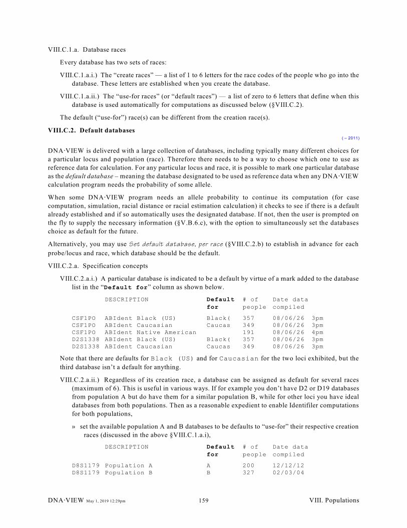
VIII.C.1.a. Database races
Every database has two sets of races:
VIII.C.1.a.i.) The “create races” — a list of 1 to 6 letters for the race codes of the people who go into the
database. These letters are established when you create the database.
VIII.C.1.a.ii.) The “use-for races” (or “default races”) — a list of zero to 6 letters that define when this
database is used automatically for computations as discussed below (§VIII.C.2).
The default (“use-for”) race(s) can be different from the creation race(s).
VIII.C.2. Default databases( – 2011)
DNA@VIEW is delivered with a large collection of databases, including typically many different choices for
a particular locus and population (race). Therefore there needs to be a way to choose which one to use as
reference data for calculation. For any particular locus and race, it is possible to mark one particular database
as the default database – meaning the database designated to be used as reference data when any DNA@VIEW
calculation program needs the probability of some allele.
When some DNA@VIEW program needs an allele probability to continue its computation (for case
computation, simulation, racial distance or racial estimation calculation) it checks to see if there is a default
already established and if so automatically uses the designated database. If not, then the user is prompted on
the fly to supply the necessary information (§V.B.6.c), with the option to simultaneously set the databases
choice as default for the future.
Alternatively, you may use Set default database, per race (§VIII.C.2.b) to establish in advance for each
probe/locus and race, which database should be the default.
VIII.C.2.a. Specification concepts
VIII.C.2.a.i.) A particular database is indicated to be a default by virtue of a mark added to the database
list in the “Default for” column as shown below.
DESCRIPTION Default # of Date data
for people compiled
CSF1PO ABIdent Black (US) Black( 357 08/06/26 3pmCSF1PO ABIdent Caucasian Caucas 349 08/06/26 3pmCSF1PO ABIdent Native American 191 08/06/26 4pmD2S1338 ABIdent Black (US) Black( 357 08/06/26 3pmD2S1338 ABIdent Caucasian Caucas 349 08/06/26 3pm
Note that there are defaults for Black (US) and for Caucasian for the two loci exhibited, but the
third database isn’t a default for anything.
VIII.C.2.a.ii.) Regardless of its creation race, a database can be assigned as default for several races
(maximum of 6). This is useful in various ways. If for example you don’t have D2 or D19 databases
from population A but do have them for a similar population B, while for other loci you have ideal
databases from both populations. Then as a reasonable expedient to enable Identifiler computations
for both populations,
» set the available population A and B databases to be defaults to “use-for” their respective creation
races (discussed in the above §VIII.C.1.a.i),
DESCRIPTION Default # of Date data
for people compiled
D8S1179 Population A A 200 12/12/12D8S1179 Population B B 327 02/03/04
DNA@VIEW May 1, 2019 12:29pm VIII. Populations159
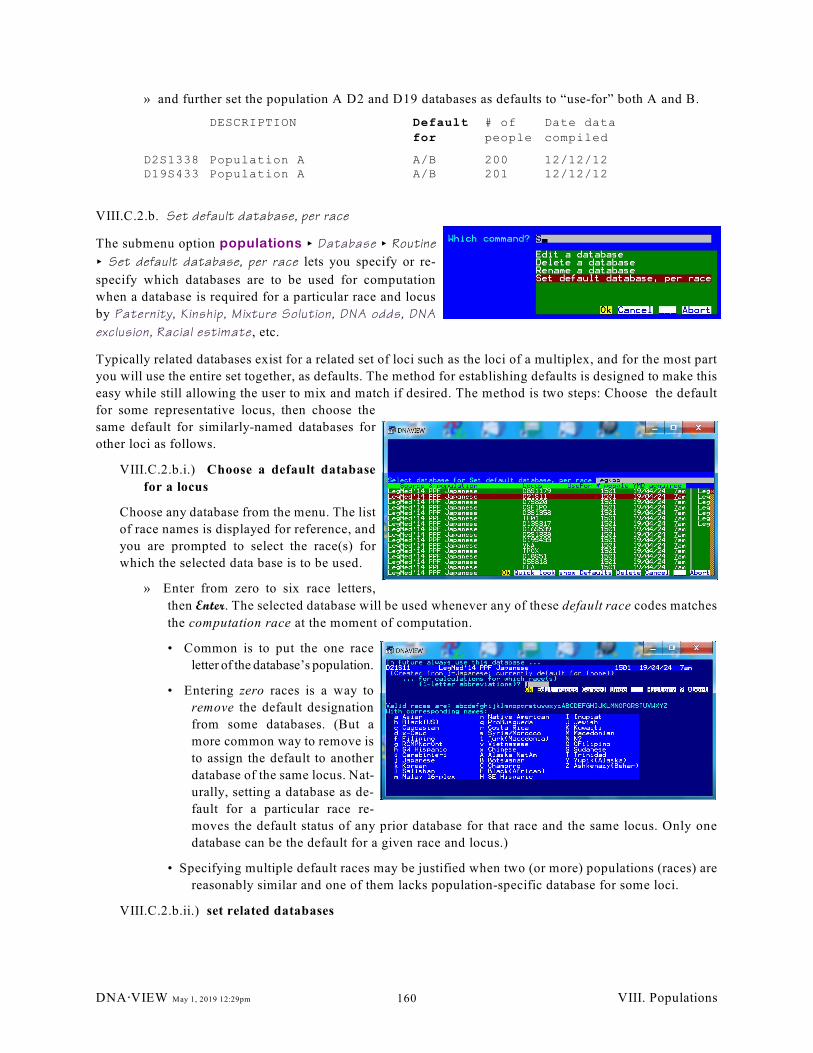
» and further set the population A D2 and D19 databases as defaults to “use-for” both A and B.
DESCRIPTION Default # of Date data
for people compiled
D2S1338 Population A A/B 200 12/12/12D19S433 Population A A/B 201 12/12/12
VIII.C.2.b. Set default database, per race
The submenu option populations < Database < Routine
< Set default database, per race lets you specify or re-
specify which databases are to be used for computation
when a database is required for a particular race and locus
by Paternity, Kinship, Mixture Solution, DNA odds, DNA
exclusion, Racial estimate, etc.
Typically related databases exist for a related set of loci such as the loci of a multiplex, and for the most part
you will use the entire set together, as defaults. The method for establishing defaults is designed to make this
easy while still allowing the user to mix and match if desired. The method is two steps: Choose the default
for some representative locus, then choose the
same default for similarly-named databases for
other loci as follows.
VIII.C.2.b.i.) Choose a default database
for a locus
Choose any database from the menu. The list
of race names is displayed for reference, and
you are prompted to select the race(s) for
which the selected data base is to be used.
» Enter from zero to six race letters,
then Enter. The selected database will be used whenever any of these default race codes matches
the computation race at the moment of computation.
• Common is to put the one race
letter of the database’s population.
• Entering zero races is a way to
remove the default designation
from some databases. (But a
more common way to remove is
to assign the default to another
database of the same locus. Nat-
urally, setting a database as de-
fault for a particular race re-
moves the default status of any prior database for that race and the same locus. Only one
database can be the default for a given race and locus.)
• Specifying multiple default races may be justified when two (or more) populations (races) are
reasonably similar and one of them lacks population-specific database for some loci.
VIII.C.2.b.ii.) set related databases
DNA@VIEW May 1, 2019 12:29pm VIII. Populations160
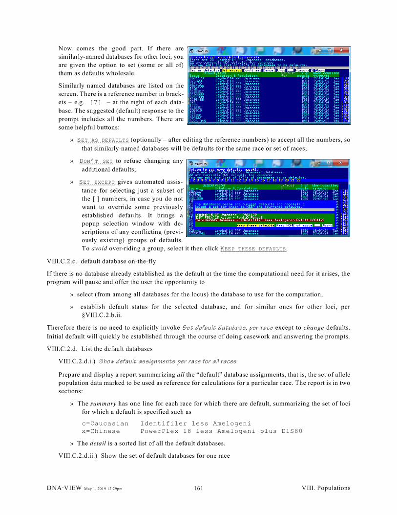
Now comes the good part. If there are
similarly-named databases for other loci, you
are given the option to set (some or all of)
them as defaults wholesale.
Similarly named databases are listed on the
screen. There is a reference number in brack-
ets – e.g. [7] – at the right of each data-
base. The suggested (default) response to the
prompt includes all the numbers. There are
some helpful buttons:
» SET AS DEFAULTS (optionally – after editing the reference numbers) to accept all the numbers, so
that similarly-named databases will be defaults for the same race or set of races;
» DON’T SET to refuse changing any
additional defaults;
» SET EXCEPT gives automated assis-
tance for selecting just a subset of
the [ ] numbers, in case you do not
want to override some previously
established defaults. It brings a
popup selection window with de-
scriptions of any conflicting (previ-
ously existing) groups of defaults.
To avoid over-riding a group, select it then click KEEP THESE DEFAULTS.
VIII.C.2.c. default database on-the-fly
If there is no database already established as the default at the time the computational need for it arises, the
program will pause and offer the user the opportunity to
» select (from among all databases for the locus) the database to use for the computation,
» establish default status for the selected database, and for similar ones for other loci, per
§VIII.C.2.b.ii.
Therefore there is no need to explicitly invoke Set default database, per race except to change defaults.
Initial default will quickly be established through the course of doing casework and answering the prompts.
VIII.C.2.d. List the default databases
VIII.C.2.d.i.) Show default assignments per race for all races
Prepare and display a report summarizing all the “default” database assignments, that is, the set of allele
population data marked to be used as reference for calculations for a particular race. The report is in two
sections:
» The summary has one line for each race for which there are default, summarizing the set of loci
for which a default is specified such as
c=Caucasian Identifiler less Amelogenix=Chinese PowerPlex 18 less Amelogeni plus D1S80
» The detail is a sorted list of all the default databases.
VIII.C.2.d.ii.) Show the set of default databases for one race
DNA@VIEW May 1, 2019 12:29pm VIII. Populations161
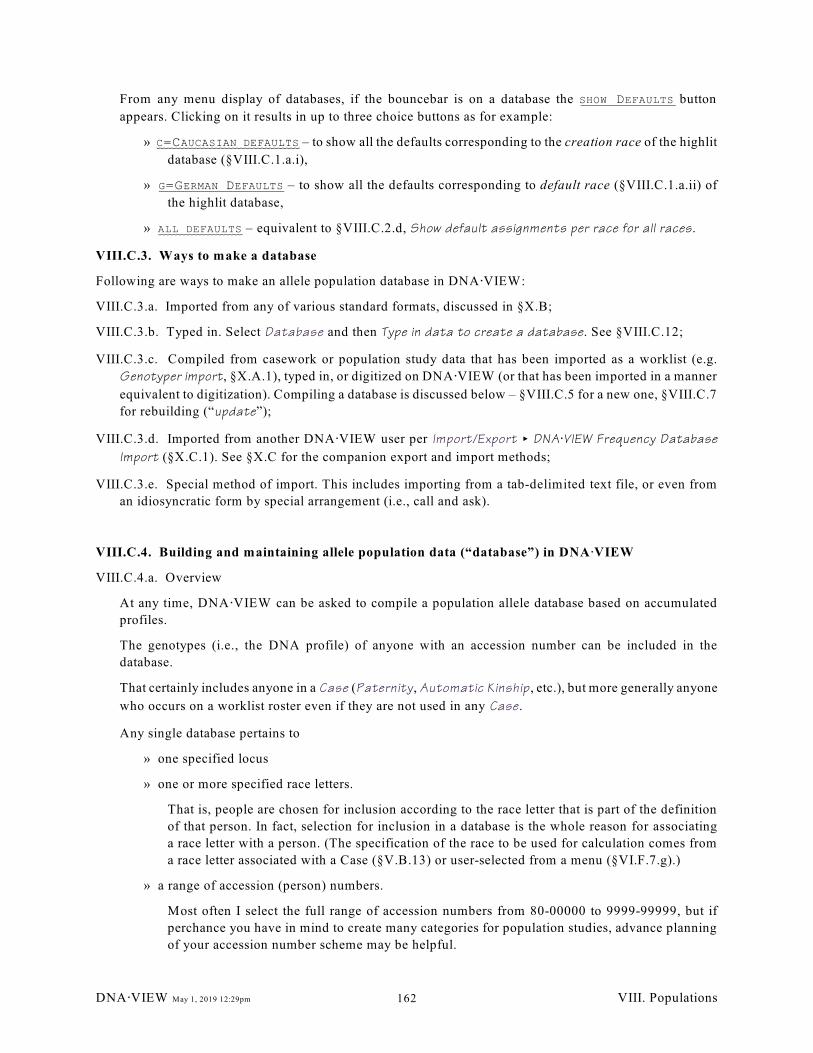
From any menu display of databases, if the bouncebar is on a database the SHOW DEFAULTS button
appears. Clicking on it results in up to three choice buttons as for example:
» C=CAUCASIAN DEFAULTS – to show all the defaults corresponding to the creation race of the highlit
database (§VIII.C.1.a.i),
» G=GERMAN DEFAULTS – to show all the defaults corresponding to default race (§VIII.C.1.a.ii) of
the highlit database,
» ALL DEFAULTS – equivalent to §VIII.C.2.d, Show default assignments per race for all races.
VIII.C.3. Ways to make a database
Following are ways to make an allele population database in DNA@VIEW:
VIII.C.3.a. Imported from any of various standard formats, discussed in §X.B;
VIII.C.3.b. Typed in. Select Database and then Type in data to create a database. See §VIII.C.12;
VIII.C.3.c. Compiled from casework or population study data that has been imported as a worklist (e.g.
Genotyper import, §X.A.1), typed in, or digitized on DNA@VIEW (or that has been imported in a manner
equivalent to digitization). Compiling a database is discussed below – §VIII.C.5 for a new one, §VIII.C.7
for rebuilding (“update”);
VIII.C.3.d. Imported from another DNA@VIEW user per Import/Export < DNA@VIEW Frequency Database
Import (§X.C.1). See §X.C for the companion export and import methods;
VIII.C.3.e. Special method of import. This includes importing from a tab-delimited text file, or even from
an idiosyncratic form by special arrangement (i.e., call and ask).
VIII.C.4. Building and maintaining allele population data (“database”) in DNA@VIEW
VIII.C.4.a. Overview
At any time, DNA @VIEW can be asked to compile a population allele database based on accumulated
profiles.
The genotypes (i.e., the DNA profile) of anyone with an accession number can be included in the
database.
That certainly includes anyone in a Case (Paternity, Automatic Kinship , etc.), but more generally anyone
who occurs on a worklist roster even if they are not used in any Case.
Any single database pertains to
» one specified locus
» one or more specified race letters.
That is, people are chosen for inclusion according to the race letter that is part of the definition
of that person. In fact, selection for inclusion in a database is the whole reason for associating
a race letter with a person. (The specification of the race to be used for calculation comes from
a race letter associated with a Case (§V.B.13) or user-selected from a menu (§VI.F.7.g).)
» a range of accession (person) numbers.
Most often I select the full range of accession numbers from 80-00000 to 9999-99999, but if
perchance you have in mind to create many categories for population studies, advance planning
of your accession number scheme may be helpful.
DNA@VIEW May 1, 2019 12:29pm VIII. Populations162
» a set of "Reader numbers" (§IX.A.5, §X.A.2.d)
The default, usually most useful, is to use all of them (099=Genotyper might be the only one)
except for 000=Student.
VIII.C.4.b. Preparation
VIII.C.4.b.i.) Routine
So keep the above in mind while designing data encoding and calculating cases. In particular, you
probably want to reserve particular letters for the likely races of interest – e.g. p for Puerto Rican. Then,
every man and every woman (but preferably not the children) should have the letter attached to their per-
son-description.
There are a few ways of doing this. You may want to use a combination.
» Assign race to an entire worklist
With Assign race to worklist (§VII.G, Disaster Analysis menu)
• select a collection of worklists;
• say whether to exclude children (probably yes);
• choose some race (letter) such as p.
Then all the denominated people will be assigned to the desired race.
» Assign race to people in a case
For each case, select the case (in Paternity case), choose edit people, and the editing cursor will
appear on the first person, the mother.
• Space twice to go past the accession number
• type e.g. p in the race cell
• tab to skip to the next person
• tab to skip past a child
• fix the (alleged) father(s) in the same way as the mother.
The most efficient practice is to make a habit of doing this while you are computing the cases.
Then the data is ready to create databases whenever you like.
» Assign race to individual people in a worklist
• Open the worklist with Worklist from the Casework menu.
• Select the lane with the person of interest.
• Space through the fields to edit the person and introduce the desired race.
VIII.C.4.b.ii.) Preliminary check
The List cases (§V.B.17) option can be used to quickly review a sequence of cases to check if you
have properly filled in the race letter for each person.
VIII.C.4.c. Compile database
Though 100 or so cases is typically regarded (for no particular reason) as a minimum size for a database,
the most efficient way is to do the initial database creation (§VIII.C.4.c.i) when you have very little or
even no profiles at all to fill them.
DNA@VIEW May 1, 2019 12:29pm VIII. Populations163
VIII.C.4.c.i.) Initial creation of databases
Even with no cases at all, you can build the (empty) databases for your lab. When you do it the first
time, there is a separate operation for each locus, so you will need 2 or 3 minutes to do all 13 or so
loci. The procedure is straightforward:
keystroke(s) reason
Pop enter Populations from main menu
D enter Database
Com enter Compile a new database from DNA@VIEW data (§VIII.C.5)
D8 enter Which locus? Select the desired locus.
Enter Which readers? Enter for default choice(s).
p Which race(s)? Type 1 to 6 letters designating races to be included in
the database.
Enter Earliest acceptable accession ID = 80-00000.
Enter Last acceptable accession ID = 9999-00000.
(time passes, probably a few seconds, and counters indicate progress as the program finds and compiles
the relevant data)
End (probably) Select the database to update, or End to make a new
one and the list of already existing databases is displayed.
Esc to proceed to the next locus.
VIII.C.4.c.ii.) Updating the databases
Once the databases have been built the first time, they can easily later be updated to reflect additional
people who have been entered into DNA@VIEW. There are two easy ways to do this.
» The first method assumes that you have marked as defaults the databases that you want to update.
If you've already been using them for casework, then this would be the case. Or, if you're
planning to use them for casework after the re-compilation, then go ahead and mark them as
defaults now, then proceed with re-compilation.
keystroke(s) reason
Pop enter Populations from main menu
D enter Database
Up enter Update the default databases (but only those marked as from your own
laboratory)
Enter Recompute these databases? y
Enter Shall I skip printing the exception reports? y
» The second method is more general, but takes (just) a few more keystrokes:
keystroke(s) reason
Pop enter Populations from main menu
D enter Database
U enter Update arbitrary list of databases
Enter Accept lines containing YourLabName
DNA@VIEW May 1, 2019 12:29pm VIII. Populations164
If desired to restrict the list further, type a context then enter (see §XIV.A.3). For example, if you are
maintaining a universal set of databases for the purpose of offender searching with the race name
anonymous,
anon enter limit the database list to the anonymous databases
Enter to accept the list
Enter Recompute these databases? y
Enter Shall I skip printing the exception reports? y
Obtain and drink coffee. Recompiling 100,000-person databases will take 1!10 minutes per locus, and
will need 10mb of RAM available to DNA·VIEW (see §XV.B.9.1).
VIII.C.5. Compile a new database from DNAAVIEW data
To compile a data base with you specify parameters to define the population of alleles to collect. See
§VIII.C.4.c.i for more operation details.
VIII.C.5.a. a locus
Which locus? D8S1179
VIII.C.5.b. the list of readers whose data to use – usually OK
VIII.C.5.c. a race (or collection of races)
VIII.C.5.d. a range of accession numbers
Earliest acceptable accession ID? 80 -00000
Last acceptable accession ID? 9999-00000
The suggested default range of accession numbers, from 80-00000 to 9999-00000, probably
includes all actual samples (particularly if you use the leading part of the accession number as a year),
while omitting “special”numbers such as 1-564 that might represent quality control samples.
Next, the program proceeds to gather all data consistent with the specified parameters, which may take some
seconds. Progress is indicated on the screen.
The data is compiled from readings of lanes labeled with an accession number in the specified range. Control
subjects and other miscellaneous lanes can be put in or left out in a variety of ways according to your choice,
depending on how you have coded the roster information for the lanes. One convenient way to omit incidental
samples from the database is to assign them a very small year number – e.g. some use 1!562 for K562
samples. Other possibilities include assigning a race code of !, or labeling the second roster column. All these
ways still permit analysis with Statistics or Quality Control.
In the case of a PCR locus or single-locus probe database, each person contributes two alleles. A homozygous
allele is counted twice. Multiple reads and/or lanes for a person are averaged (as described by algorithm
§XIII.F).
VIII.C.5.e. Filing the new database
When the new database is ready for filing, if there are any databases that you previously created for the
same locus and race(s), you will be given the option of updating an old slot with the new data, or creating
a new slot.
A menu of already existing databases for the specified locus is presented. You have three choices:
VIII.C.5.e.i.) REPLACE an existing database
DNA@VIEW May 1, 2019 12:29pm VIII. Populations165
Choose one of the already existing databases and click REPLACE. In this case before any action is taken
the two are presented side-by-side on the screen for you to compare, and you are given the option to con-
firm or change your mind, as shown in Figure 79.
(If you change your mind and choose not to overwrite the selected database, you will next be given the
option to skip filing the database altogether.)
VIII.C.5.e.ii.) CREATE NEW to add a new database in addition to those that already exist.
VIII.C.5.e.iii.) CANCEL to skip filing
VIII.C.6. Side effects
There are several side effects to compiling a data base:
< An Exception Report (see §VIII.C.8.a) is created covering any suspicious circumstances. The
report can be printed using Print. It is also saved, and can later be retrieved using Retrieve exception
report.
For a single-locus probe, suspicious circumstances include inconsistent data for any individual, such as
readings from the same lane, or from different lanes, that don’t agree to reasonable precision; inconsistent
decisions on homozygosity among different readings or lanes; and lanes that are labeled but never read,
or read only once.
In the multi-locus case, the report lists worklists with lanes read more than once, and people with data
from more than one lane.
< [PCR- or single-locus] A special record is made and saved of homozygotes, which may be
examined using the List of homozygotes (§VIII.C.11) sub-menu option of the Database command.
< [PCR- or single-locus] A special record is made of individuals run more than once — i.e. on
several worklists or lanes. See Printout of a database (§VIII.C.13).
VIII.C.7. Updating
Updating a database means to recompile a database as a collection of profiles available in among your own
data – case data and/or orphan profiles. Updating is in effect a way to re-run Compile a new database from
DNA·VIEW data (§VIII.C.5) automatically and en masse. Hence it is only possible for database that were
compiled locally per §VIII.C.5. Updating imported databases, whether shared from another DNA@VIEW
installation per §X.C.1 or imported per §X.B, is not possible.
Since you may often want to update all or many of your databases at the same time and there are likely to be
quite a few of them (one for each probe-race combination), several options are available for convenience.
VIII.C.7.a. Update the default databases lets DNA·VIEW take over the keyboard and automatically
replaces each database that is
(a) marked as a default, and
(b) is from your own laboratory.
Each newly compiled database then replaces the older version.
VIII.C.7.b. Update arbitrary list of databases first lets you select an arbitrary collection of databases. The
method of selection is by contextual phrases, as described under §XIV.A.3, “Multiple selection”.
DNA·VIEW then takes over the keyboard, recomputes each specified database, and replaces the old
version with the new one.
DNA@VIEW May 1, 2019 12:29pm VIII. Populations166
Exception reports are automatically printed out for each recompiled database under either of the last two
options. But if you want to save paper you can temporarily change the printer to (none) (see §IX.F.9).
VIII.C.7.c. Detail remarks about updating
The updated version is compiled based on the same race(s), accession number range, and probe number
as were specified for the previous version. DNA@VIEW suggests the accession number range of
80-00000 to 9999-00000 when you initially create a database so that it will be convenient to use the
Update method to create ever more inclusive versions.
Also, if you have manually changed the name of the database, your new name will be retained after the
update.
The set of readers, however, is not remembered from the previous database compilation. Rather, the
updated database is always based on the default set of readers which is those numbered from 1 to 999.
STUDENT (000) is therefore omitted, as would be any irregular readers (since normally there aren’t any)
with numbers 1000 and above.
VIII.C.8. Review exception report
This is an obsolescent option mainly intended for RFLP. For most of the description, see an old version of
the manual.
VIII.C.8.a. 3-banded patterns
The exception report includes a list of people with 3 bands.
VIII.C.9. Delete or rename
to select a data base for deletion or to rename. As usual, you are asked to confirm your selection before the
data base is deleted. If you do not confirm deletion, then you are given a prompt to rename it.
VIII.C.10. Combine
lets you create a single database as a combination of several. Two likely reasons to do this:
» combine databases from several different laboratories into one larger one,
» combine a database compiled with DNA@VIEW and one entered by typing.
An important point to appreciate: Suppose that you have created a database without DNA@VIEW,
then you acquire DNA@VIEW and after a time have accumulated data in DNA@VIEW that you would
like to add to your earlier data. Do not select the typed in database for “updating.” That would simply
replace the typed-in data with the accumulated data. The only method that works is to create three
databases: The typed-in one, a second one from the DNA@VIEW data, and a third one of the
combined data.
VIII.C.10.b. Example steps for combining databases:
populations < Database < Construct < Create a combination of databases
First Combination of databases component? Choose a database, OK
Additional ... component? Choose a database, OK
Additional ... component? Choose a database, OK
Additional ... component? DONE
(# of people) OK; repeat for each component.Is all the information correct? yCreate a new database or replace an existing one.
edit the name [retype if you like] OK
DNA@VIEW May 1, 2019 12:29pm VIII. Populations167
VIII.C.11. List of homozygotes
As a side effect of compiling allele frequencies (see Database, Compile ... or Update ...),a record is saved of
all people for whom only one allele was digitized. The list of their accession numbers can be retrieve using
this sub-menu option, then printed with Print.
The accession number lists for several data bases with the same probe may be combined into a single sorted
list.
Accession numbers are not available for imported data bases compiled at a foreign site.
VIII.C.12. Edit or type in a database
Editing a database is done with a friendly full-screen editor. Features include:
» Edit an existing one, or create a new one and type in the alleles and count of occurrences.
» PCR allele notation or base pair notation both allowed
» Search for sizes, and automatic scrolling.
» Automatic scaling allows you to enter data from a table that gives decimal frequencies (enter on a
per-thousand basis), then adjust the frequencies to an allele-count basis by changing the total to the
correct total number.
VIII.C.12.b. Allele name and count
The input screen requires allele name (allele number for STR, letter codes for SNP’s, Amelogenin, or poly-
markers, base pairs for RFLP) and count – not frequency. However, if you have a source document that lists
frequencies, it is easy to make the program do the conversion.
VIII.C.12.c. Protocol that converts frequency to count
Suppose for example that the input document lists the 3-allele population sample shown in Figure 79, not
explicitly listing the actual "counts." However, that is no problem. for here's a simple trick. Enter the decimal
number scaled by 1000 – i.e. enter the database on the basis of n=1000 alleles, as shown at the right:
Then, at the bottom of the screen where it says “Total alleles”, change the scaled total of 999 to the correct
number, 114. The numbers for allele count automatically change proportionally.
Now, click Save and exit, and the computer will round to the exactly correct values – 3, 12, 99 – and
save them.
VIII.C.12.d. Automatic conversion of frequency to count
Alternatively, you may enter or scale the numbers to actual frequencies (total alleles =1). Then click Save
and exit and a dialogue, beginning with the program's plausible guess as to the correct total, guides you
through conversion of frequency to count.
VIII.C.12.e. Null alleles
Null alleles are handled in DNAAVIEW by adding a count to a database. To enter null alleles, type the letter
n in the allele column, then an appropriate count in the count column.
DNA@VIEW May 1, 2019 12:29pm VIII. Populations168
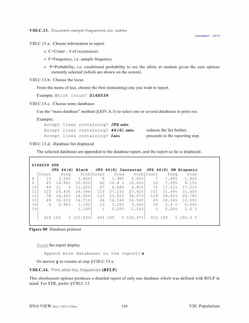
D16S539 STR
JFS 44(6) Black JFS 44(6) Caucasian JFS 44(6) SW Hispanic *Count Freq Prob*Count Freq Prob*Count Freq Prob8 * 15 3.59% 3.82%* 8 1.98% 2.22%* 7 1.68% 1.92%9 * 83 19.86% 20.05%* 42 10.4 % 10.62%* 33 7.93% 8.15%10* 46 11 % 11.22%* 27 6.68% 6.91%* 72 17.31% 17.51%11* 123 29.43% 29.59%* 110 27.23% 27.41%* 131 31.49% 31.65%12* 78 18.66% 18.85%* 137 33.91% 34.07%* 119 28.61% 28.78%13* 69 16.51% 16.71%* 66 16.34% 16.54%* 43 10.34% 10.55%14* 4 0.96% 1.19%* 13 3.22% 3.46%* 10 2.4 % 2.64%15* 1.19%* 1 0.25% 1.23%* 1 0.24% 1.2 % * * * * 418 100 % 102.63%* 404 100 % 102.47%* 416 100 % 102.4 %
Figure 80 Database printout
VIII.C.13. Document sample frequencies etc. tables (redesigned – 2011)
VIII.C.13.a. Choose information to report
» C=Count – # of occurrences
» F=Frequency, i.e. sample frequency
» P=Probability, i.e. conditional probability to see the allele at random given the user options
currently selected (which are shown on the screen)
VIII.C.13.b. Choose the locus
From the menu of loci, choose the first (remaining) one you wish to report.
Example: Which locus? D16S539
VIII.C.13.c. Choose some databases
Use the “mass database” method (§XIV.A.3) to select one or several databases to print out.
Example:
Accept lines containing? JFS enter
Accept lines containing? 44(6) enter reduces the list further.
Accept lines containing? Enter proceeds to the reporting step.
VIII.C.13.d. Database list displayed
The selected databases are appended to the database report, and the report so far is displayed.
CLOSE the report display
Append more databases to the report? n
Or answer y to resume at step §VIII.C.13.a.
VIII.C.14. Print allele list, frequencies (RFLP)
This obsolescent options produces a detailed report of only one database which was defined with RFLP in
mind. For STR, prefer §VIII.C.13.
DNA@VIEW May 1, 2019 12:29pm VIII. Populations169
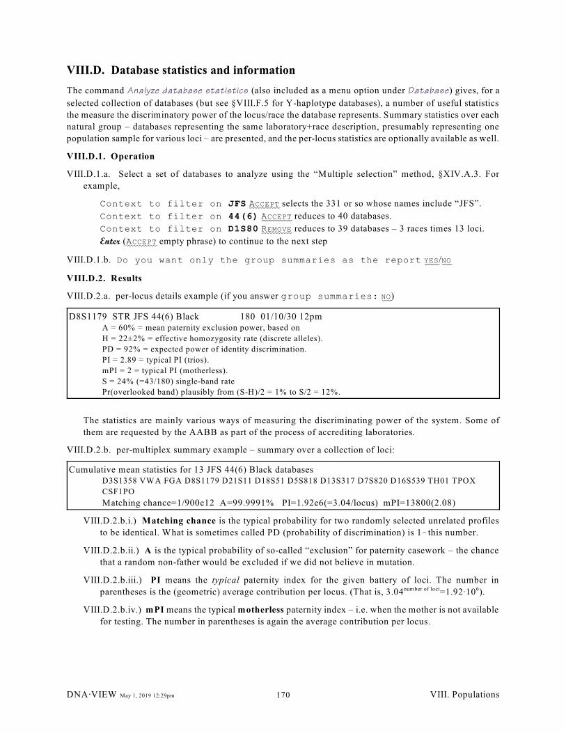
D8S1179 STR JFS 44(6) Black 180 01/10/30 12pmA = 60% = mean paternity exclusion power, based on
H = 22±2% = effective homozygosity rate (discrete alleles).
PD = 92% = expected power of identity discrimination.
PI = 2.89 = typical PI (trios).
mPI = 2 = typical PI (motherless).
S = 24% (=43/180) single-band rate
Pr(overlooked band) plausibly from (S-H)/2 = 1% to S/2 = 12%.
Cumulative mean statistics for 13 JFS 44(6) Black databasesD3S1358 VWA FGA D8S1179 D21S11 D18S51 D5S818 D13S317 D7S820 D16S539 TH01 TPOX
CSF1PO
Matching chance=1/900e12 A=99.9991% PI=1.92e6(=3.04/locus) mPI=13800(2.08)
VIII.D. Database statistics and information
The command Analyze database statistics (also included as a menu option under Database) gives, for a
selected collection of databases (but see §VIII.F.5 for Y-haplotype databases), a number of useful statistics
the measure the discriminatory power of the locus/race the database represents. Summary statistics over each
natural group – databases representing the same laboratory+race description, presumably representing one
population sample for various loci – are presented, and the per-locus statistics are optionally available as well.
VIII.D.1. Operation
VIII.D.1.a. Select a set of databases to analyze using the “Multiple selection” method, §XIV.A.3. For
example,
Context to filter on JFS ACCEPT selects the 331 or so whose names include “JFS”.
Context to filter on 44(6) ACCEPT reduces to 40 databases.
Context to filter on D1S80 REMOVE reduces to 39 databases – 3 races times 13 loci.
Enter (ACCEPT empty phrase) to continue to the next step
VIII.D.1.b. Do you want only the group summaries as the report YES/NO
VIII.D.2. Results
VIII.D.2.a. per-locus details example (if you answer group summaries: NO)
The statistics are mainly various ways of measuring the discriminating power of the system. Some of
them are requested by the AABB as part of the process of accrediting laboratories.
VIII.D.2.b. per-multiplex summary example – summary over a collection of loci:
VIII.D.2.b.i.) Matching chance is the typical probability for two randomly selected unrelated profiles
to be identical. What is sometimes called PD (probability of discrimination) is 1!this number.
VIII.D.2.b.ii.) A is the typical probability of so-called “exclusion” for paternity casework – the chance
that a random non-father would be excluded if we did not believe in mutation.
VIII.D.2.b.iii.) PI means the typical paternity index for the given battery of loci. The number in
parentheses is the (geometric) average contribution per locus. (That is, 3.04 =1.92A10 ).number of loci 6
VIII.D.2.b.iv.) mPI means the typical motherless paternity index – i.e. when the mother is not available
for testing. The number in parentheses is again the average contribution per locus.
DNA@VIEW May 1, 2019 12:29pm VIII. Populations170
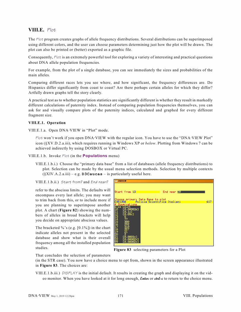
Figure 83 selecting parameters for a Plot
VIII.E. Plot
The Plot program creates graphs of allele frequency distributions. Several distributions can be superimposed
using different colors, and the user can choose parameters determining just how the plot will be drawn. The
plot can also be printed or (better) exported as a graphic file.
Consequently, Plot is an extremely powerful tool for exploring a variety of interesting and practical questions
about DNA allele population frequencies.
For example, from the plot of a single database, you can see immediately the sizes and probabilities of the
main alleles.
Comparing different races lets you see where, and how significant, the frequency differences are. Do
Hispanics differ significantly from coast to coast? Are there perhaps certain alleles for which they differ?
Artfully drawn graphs tell the story clearly.
A practical test as to whether population statistics are significantly different is whether they result in markedly
different calculations of paternity index. Instead of comparing population frequencies themselves, you can
ask for and visually compare plots of the paternity indices, calculated and graphed for every different
fragment size.
VIII.E.1. Operation
VIII.E.1.a. Open DNA@VIEW in “Plot” mode.
Plot won’t work if you open DNA@VIEW with the regular icon. You have to use the “DNA@VIEW Plot”
icon (§XV.D.2.a.iii), which requires running in Windows XP or below. Plotting from Windows 7 can be
achieved indirectly by using DOSBOX or Virtual PC.
VIII.E.1.b. Invoke Plot (in the Populations menu)
VIII.E.1.b.i.) Choose the “primary data base” from a list of databases (allele frequency distributions) to
plot. Selection can be made by the usual menu selection methods. Selection by multiple contexts
(§XIV.A.2.a.iii) – e.g. D3Caucas – is particularly useful here.
VIII.E.1.b.ii.) Start from? and End near?
refer to the abscissa limits. The defaults will
encompass every last allele; you may want
to trim back from this, or to include more if
you are planning to superimpose another
plot. A chart (Figure 82) showing the num-
bers of alleles in broad brackets will help
you decide on appropriate abscissa values.
The bracketed %’s (e.g. [0.1%]) in the chart
indicate alleles not present in the selected
database and show what is their overall
frequency among all the installed population
studies.
That concludes the selection of parameters
(in the STR case). You now have a choice menu to opt from, shown in the screen appearance illustrated
in Figure 83. The choices are:
VIII.E.1.b.iii.) DISPLAY is the initial default. It results in creating the graph and displaying it on the vid-
eo monitor. When you have looked at it for long enough, Enter or ctrl-c to return to the choice menu.
DNA@VIEW May 1, 2019 12:29pm VIII. Populations171
VIII.E.1.b.iv.) PRINTER – A (not very attractive) copy of the graph is printed on the printer. A better
option:
VIII.E.1.b.v.) L L METAFIL – to create an editable graphic file for use in a publication or other
document
A coded image of the graph is written to a file. The file format is called CGI or CGM. It can be
imported into Word, Powerpoint etc., or edited with a graphics program such as Corel Draw.
VIII.E.1.b.vi.) start over – Go back to the beginning of Plot, except that the choices you made pre-
viously will be remembered and used as defaults.
VIII.E.1.b.vii.) quit – Exit from Plot.
VIII.E.1.b.viii.) more plots – Get another database to superimpose onto the graph.
If you select a database that is already included in the graph, the prompt smooth by? – intended
for RFLP databases – offers to simulate measurement uncertainty.
VIII.E.1.b.ix.) fewer plots lets you back up by removing a database from the plot.
VIII.E.1.b.x.) homozygotes – similar to more plots, but the graph is of just the homozygous individuals
found for the given probe. This information is usually available only for data compiled by DNA·
VIEW, as opposed to data that was typed in.
VIII.E.1.b.xi.) paternity index creates a special superimposed plot consisting of the paternity index
calculated point by point by considering in turn each size on the X-axis to be the obligatory paternal
size for a typical paternity case.
As a useful side effect, the graph legend will report the “typical PI” (geometric mean, see Brenner
& Morris (1989), page 36).
Notes on scales: If one or more graphs of paternity index are requested, then the Y-axis is labeled
with the PI. The PI’s will be packed close together toward the top of the screen, so that an infinite
PI corresponds to the top margin.
VIII.E.1.b.xii.) turn histogram on/off – This option is only for demonstration when displaying RFLP
data.
VIII.E.2. Experimental Plot features
The features mentioned in this section are not meant to be counted as part of the DNA·VIEW product. They
are not guaranteed to work, nor to persist in future versions. The descriptions are in most cases admittedly
and intentionally sketchy.
VIII.E.2.a. Modify Plot Colors
While looking at a plot, you can modify the colors.
Sketchy background information: Each color is a mixture of Red, Green, and Blue, intensities ranging
from 0!1000, and these intensities are typed in using the letters a!z. Each color in the plot has a number,
0, 1, 2, 3, 4, 5, 6, 7, 8, 9, A, B, C, D, E, F. 0 is the background, 2 & 3 are the grid, 4 the centered caption,
5,6,... the colors of the individual graphs.
As you are changing the colors, there is some coded feedback in the lower right hand corner of the screen.
Space makes it disappear.
Examples: 5zaa changes color 5 to solid red. Then ufo changes color 5 to fuchsia. Now hit ! or + and
watch the red intensity diminish or increase. Type . to advance to the next primary constituent. 0;1
exchanges colors 0 and 1. / and \ restore the current color, and all colors, to their values at the beginning
DNA@VIEW May 1, 2019 12:29pm VIII. Populations172
of the plot. # switches to an alternate palette. This is necessary before printing to a color printer if you
want a white (unpainted) background.
The key ! creates a gradation of intensities merging to the background. $ undulates the colors over time.
VIII.E.2.b. Show Marker Sizes (RFLP feature)
Marker sizes can be superimposed on the plot by choosing the option Ladder from the option menu.
VIII.E.2.c. Comparing Different Smoothings (RFLP feature)
If you choose the Plot option more plots and choose a plot that’s already been chosen, DNA·VIEW
suspects you want to use a different smoothing the second time, and gives you an opportunity to specify
it.
DNA@VIEW May 1, 2019 12:29pm VIII. Populations173
VIII.F. Y haplotypes in DNA@VIEW
improved
VIII.F.1. Y haplotype overview
new
VIII.F.1.a. Y haplotypes
The Y haplotype for an individual is the alleles for a collection of loci on the Y chromosome. Importing
Y haplotypes is therefore the same as importing autosomal data – specify the alleles for some loci.
For calculation and “databases” though Y haplotypes of course need to be treated as a haplotype unit,
never as individual loci, and this is quite different from the treatment of autosomal (or X-linked) loci in
DNA@VIEW.
VIII.F.1.b. Y loci
Some collections of Y loci, such as YFiler, are included in the multiplex list (§IX.B.7). However, any
arbitrary set of Y loci is allowed to comprise a Y haplotype. Any locus is considered by the program to
be a Y locus or not according to the genetic type (§IX.B.3.f) coding associated with the locus.
VIII.F.1.c. What are Y haplotype databases?
A DNA@VIEW Y-haplotype database consists of a population sample – a collection – of Y-haplotypes
from test subjects, for a particular racial category.
Y-haplotype databases are different from single-locus (autosomal or X) databases. There is a special list
of Y-haplotype database, and the ways to manipulate, maintain, and use the Y haplotype databases are
quite different from the autosomal database facilities.
You may have Y-haplotype databases for as many populations as you wish. Each database
! has identifying parameters
" race (a race letter)
" name (arbitrary text description)
! haplotypes
" for any set of Y-loci
" any number of individuals
- incomplete haplotypes (missing locus here and there) are allowed
- multiple alleles per locus are not allowed as of now
It’s permitted to have several Y-haplotype databases associated with the same race. The first database for
a given race letter has priority. Therefore the order of the databases (§VIII.F.4.a.i) is significant.
VIII.F.1.d. Y haplotypes for identification
Several DNA@VIEW programs use Y haplotypes in computation.
VIII.F.1.d.i.) Crime stain matching
Y-haplotype matching LR (§V.H) looks up a given haplotype in the Y haplotype databases and
reports the evidential value of a match.
VIII.F.1.d.ii.) Kinship and body identification
A Y haplotype LR can be incorporated into a kinship calculation. Some pairwise matching LR tables
include Y haplotype evidence. See §VI.F.5 Y in kinship.
VIII.F.1.d.iii.) Disaster screening
DNA@VIEW May 1, 2019 12:29pm VIII. Populations174
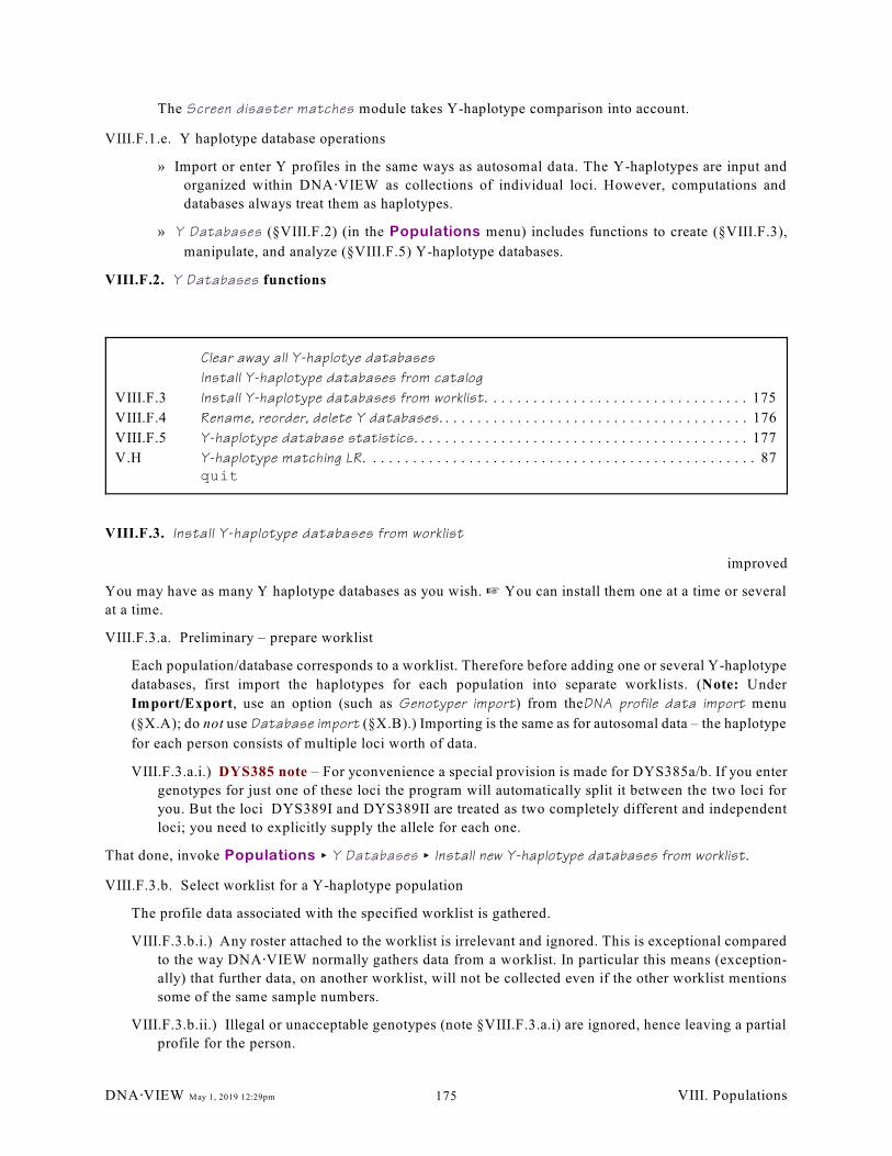
Clear away all Y-haplotye databases
Install Y-haplotype databases from catalog
VIII.F.3 Install Y-haplotype databases from worklist. . . . . . . . . . . . . . . . . . . . . . . . . . . . . . . . . 175
VIII.F.4 Rename, reorder, delete Y databases. . . . . . . . . . . . . . . . . . . . . . . . . . . . . . . . . . . . . . . 176
VIII.F.5 Y-haplotype database statistics. . . . . . . . . . . . . . . . . . . . . . . . . . . . . . . . . . . . . . . . . . 177
V.H Y-haplotype matching LR. . . . . . . . . . . . . . . . . . . . . . . . . . . . . . . . . . . . . . . . . . . . . . . . . 87quit
The Screen disaster matches module takes Y-haplotype comparison into account.
VIII.F.1.e. Y haplotype database operations
» Import or enter Y profiles in the same ways as autosomal data. The Y-haplotypes are input and
organized within DNA@VIEW as collections of individual loci. However, computations and
databases always treat them as haplotypes.
» Y Databases (§VIII.F.2) (in the Populations menu) includes functions to create (§VIII.F.3),
manipulate, and analyze (§VIII.F.5) Y-haplotype databases.
VIII.F.2. Y Databases functions
VIII.F.3. Install Y-haplotype databases from worklist
improved
You may have as many Y haplotype databases as you wish. L You can install them one at a time or several
at a time.
VIII.F.3.a. Preliminary – prepare worklist
Each population/database corresponds to a worklist. Therefore before adding one or several Y-haplotype
databases, first import the haplotypes for each population into separate worklists. (Note: Under
Import/Export, use an option (such as Genotyper import) from theDNA profile data import menu
(§X.A); do not use Database import (§X.B).) Importing is the same as for autosomal data – the haplotype
for each person consists of multiple loci worth of data.
VIII.F.3.a.i.) DYS385 note – For yconvenience a special provision is made for DYS385a/b. If you enter
genotypes for just one of these loci the program will automatically split it between the two loci for
you. But the loci DYS389I and DYS389II are treated as two completely different and independent
loci; you need to explicitly supply the allele for each one.
That done, invoke Populations < Y Databases < Install new Y-haplotype databases from worklist.
VIII.F.3.b. Select worklist for a Y-haplotype population
The profile data associated with the specified worklist is gathered.
VIII.F.3.b.i.) Any roster attached to the worklist is irrelevant and ignored. This is exceptional compared
to the way DNA@VIEW normally gathers data from a worklist. In particular this means (exception-
ally) that further data, on another worklist, will not be collected even if the other worklist mentions
some of the same sample numbers.
VIII.F.3.b.ii.) Illegal or unacceptable genotypes (note §VIII.F.3.a.i) are ignored, hence leaving a partial
profile for the person.
DNA@VIEW May 1, 2019 12:29pm VIII. Populations175
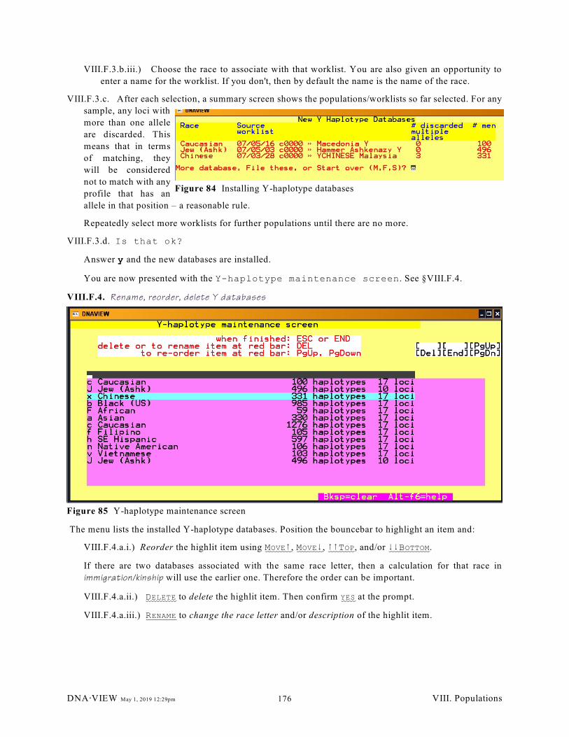
Figure 84 Installing Y-haplotype databases
Figure 85 Y-haplotype maintenance screen
VIII.F.3.b.iii.) Choose the race to associate with that worklist. You are also given an opportunity to
enter a name for the worklist. If you don't, then by default the name is the name of the race.
VIII.F.3.c. After each selection, a summary screen shows the populations/worklists so far selected. For any
sample, any loci with
more than one allele
are discarded. This
means that in terms
of matching, they
will be considered
not to match with any
profile that has an
allele in that position – a reasonable rule.
Repeatedly select more worklists for further populations until there are no more.
VIII.F.3.d. Is that ok?
Answer y and the new databases are installed.
You are now presented with the Y-haplotype maintenance screen. See §VIII.F.4.
VIII.F.4. Rename, reorder, delete Y databases
The menu lists the installed Y-haplotype databases. Position the bouncebar to highlight an item and:
VIII.F.4.a.i.) Reorder the highlit item using MOVE8, MOVE9, 88TOP, and/or 99BOTTOM.
If there are two databases associated with the same race letter, then a calculation for that race in
immigration/kinship will use the earlier one. Therefore the order can be important.
VIII.F.4.a.ii.) DELETE to delete the highlit item. Then confirm YES at the prompt.
VIII.F.4.a.iii.) RENAME to change the race letter and/or description of the highlit item.
DNA@VIEW May 1, 2019 12:29pm VIII. Populations176
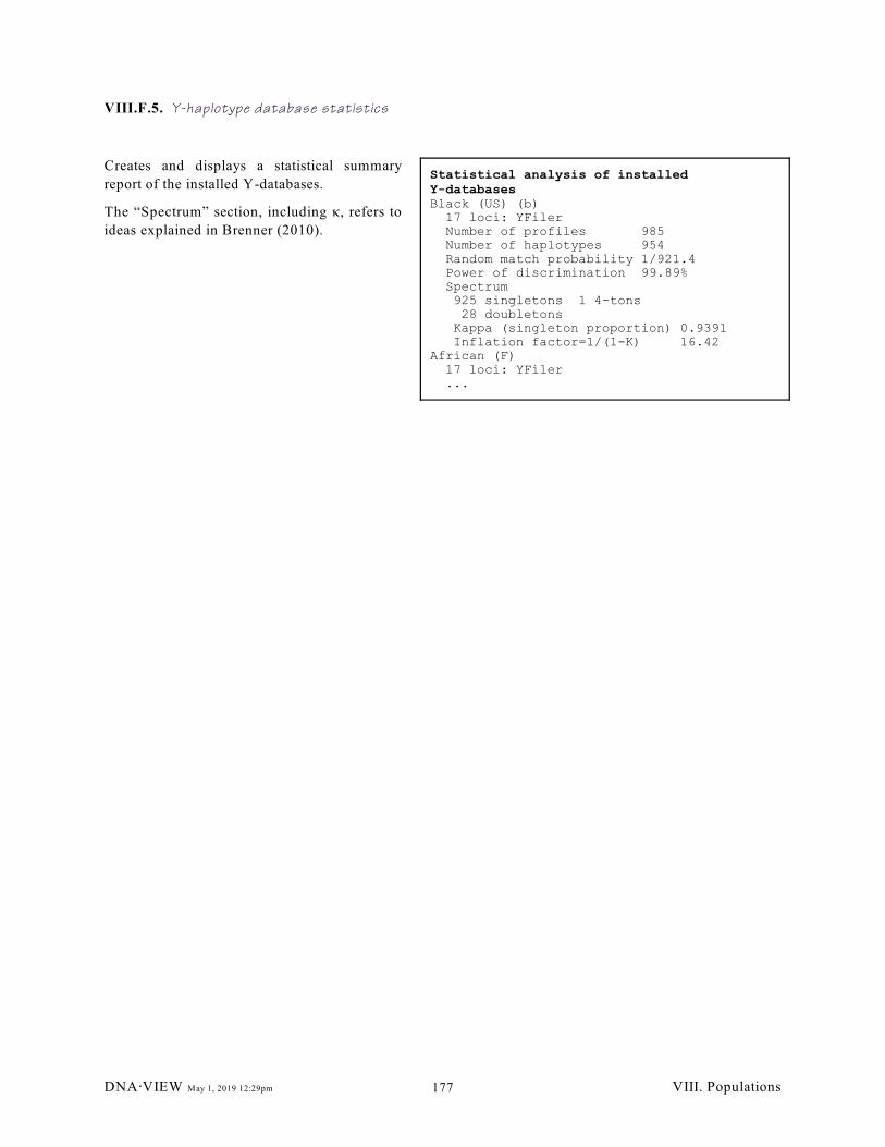
Statistical analysis of installedY-databasesBlack (US) (b) 17 loci: YFiler Number of profiles 985 Number of haplotypes 954 Random match probability 1/921.4 Power of discrimination 99.89% Spectrum 925 singletons 1 4-tons 28 doubletons Kappa (singleton proportion) 0.9391 Inflation factor=1/(1-K) 16.42African (F) 17 loci: YFiler ...
VIII.F.5. Y-haplotype database statistics
Creates and displays a statistical summary
report of the installed Y-databases.
The “Spectrum” section, including ê, refers to
ideas explained in Brenner (2010).
DNA@VIEW May 1, 2019 12:29pm VIII. Populations177
VIII.G. Exact Tests for Independence
This section is a background discussion for the programs which are described in the following sections.
Some forensic calculations — including paternity calculations — implicitly assume that alleles are randomly
assorted through the population. DNA@VIEW includes commands implementing the statistical tests of Guo
(1992) and Zaykin (1995) to test for random assortment.
Multiplication of paternity indices or of matching LRs between loci is valid only to the extent that the loci
are independent. Independence might be violated if loci are physically linked or by reason of non-random
mating.
To say independence between loci holds for an infinite population means that for each allele b at locus B and
each allele c at locus C, b occurs at the same rate among people who have c as it does among all people. In
practice it is necessary to test this hypothesis with only a finite sample of people, for whom some variation
from the ideal proportions inevitably occurs because of sampling variation — i.e. chance. The question for
a statistical test, then, is this: How likely is the observed variation to occur just because of sampling variation,
even when the independence hypothesis holds?
VIII.G.1.a. Logic
Independence is a property of a population, but in practice we only test a sample (subset) of a population.
Therefore, in typical statistical language, the test result can never be definitive, but only says whether there
is evidence of non-independence based on the sample.
For major populations it is by now well established that independent assortment of alleles is close to true but
not exactly true. In the early 1990's there was a debate in the forensic community – or perhaps a debate
between the forensic and parts of the legal community. One side alleged that the populations must be in
equilibrium so the product rule for DNA probabilities is accurate, the other side that the product rule may be
far from true and traditional DNA probability calculations completely unfair and unjustified. I think it is now
clear that the truth is in between: completely random assortment is a fiction, but real populations come close.
However, unfortunately there is no particular relationship between “passing” the exact test and sufficient
accuracy of the product rule. Passing could and does simply mean not enough data was examined.
Conversely, if we examined sufficiently large population samples – of 10000+ individuals would be my guess
– then we would see clearcut statistical evidence of non-independence, even though the magnitude of the
departure from independence is probably forensically unimportant.
In summary, these tests are less valuable for database “validation” purposes than I thought when I
implemented them. They do still serve some limited purposes:
VIII.G.1.a.i.) Errors in compiling the data sometimes show up as vast departures from statistical
independence. Hence, failure of these tests may point to systemic errors.
VIII.G.1.a.ii.) When loci are quite close – e.g. when one is evaluating potential new forensic loci such
as SNP sites – there can still be a real question of independence or not.
VIII.G.1.a.iii.) The forensic literature is still adding to the large volume of database papers using
pointless “validation” methods, and you can check them or imitate them if you like.
VIII.G.1.b. Exact test for independence of loci
The so-called “exact test” for independence of loci is described in Zaykin et al (1995). As described in
the paper, the following choices are allowed for consideration of each locus:
VIII.G.1.b.i.) assuming that the sample will necessarily have the same allele counts as this sample does,
what is the probability p to observe exactly this set of (multi-locus) genotypes?
DNA@VIEW May 1, 2019 12:29pm VIII. Populations178
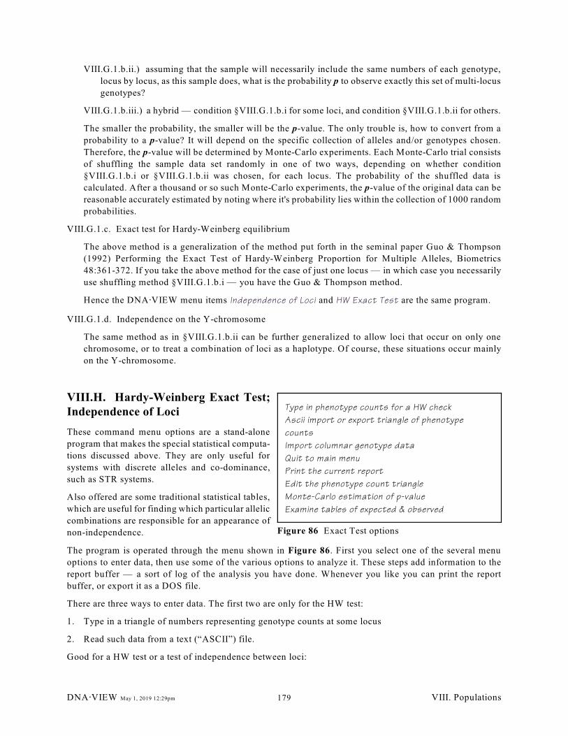
Type in phenotype counts for a HW check
Ascii import or export triangle of phenotype
counts
Import columnar genotype data
Quit to main menu
Print the current report
Edit the phenotype count triangle
Monte-Carlo estimation of p-value
Examine tables of expected & observed
Figure 86 Exact Test options
VIII.G.1.b.ii.) assuming that the sample will necessarily include the same numbers of each genotype,
locus by locus, as this sample does, what is the probability p to observe exactly this set of multi-locus
genotypes?
VIII.G.1.b.iii.) a hybrid — condition §VIII.G.1.b.i for some loci, and condition §VIII.G.1.b.ii for others.
The smaller the probability, the smaller will be the p-value. The only trouble is, how to convert from a
probability to a p-value? It will depend on the specific collection of alleles and/or genotypes chosen.
Therefore, the p-value will be determined by Monte-Carlo experiments. Each Monte-Carlo trial consists
of shuffling the sample data set randomly in one of two ways, depending on whether condition
§VIII.G.1.b.i or §VIII.G.1.b.ii was chosen, for each locus. The probability of the shuffled data is
calculated. After a thousand or so such Monte-Carlo experiments, the p-value of the original data can be
reasonable accurately estimated by noting where it's probability lies within the collection of 1000 random
probabilities.
VIII.G.1.c. Exact test for Hardy-Weinberg equilibrium
The above method is a generalization of the method put forth in the seminal paper Guo & Thompson
(1992) Performing the Exact Test of Hardy-Weinberg Proportion for Multiple Alleles, Biometrics
48:361-372. If you take the above method for the case of just one locus — in which case you necessarily
use shuffling method §VIII.G.1.b.i — you have the Guo & Thompson method.
Hence the DNA@VIEW menu items Independence of Loci and HW Exact Test are the same program.
VIII.G.1.d. Independence on the Y-chromosome
The same method as in §VIII.G.1.b.ii can be further generalized to allow loci that occur on only one
chromosome, or to treat a combination of loci as a haplotype. Of course, these situations occur mainly
on the Y-chromosome.
VIII.H. Hardy-Weinberg Exact Test;Independence of Loci
These command menu options are a stand-alone
program that makes the special statistical computa-
tions discussed above. They are only useful for
systems with discrete alleles and co-dominance,
such as STR systems.
Also offered are some traditional statistical tables,
which are useful for finding which particular allelic
combinations are responsible for an appearance of
non-independence.
The program is operated through the menu shown in Figure 86. First you select one of the several menu
options to enter data, then use some of the various options to analyze it. These steps add information to the
report buffer — a sort of log of the analysis you have done. Whenever you like you can print the report
buffer, or export it as a DOS file.
There are three ways to enter data. The first two are only for the HW test:
1. Type in a triangle of numbers representing genotype counts at some locus
2. Read such data from a text (“ASCII”) file.
Good for a HW test or a test of independence between loci:
DNA@VIEW May 1, 2019 12:29pm VIII. Populations179
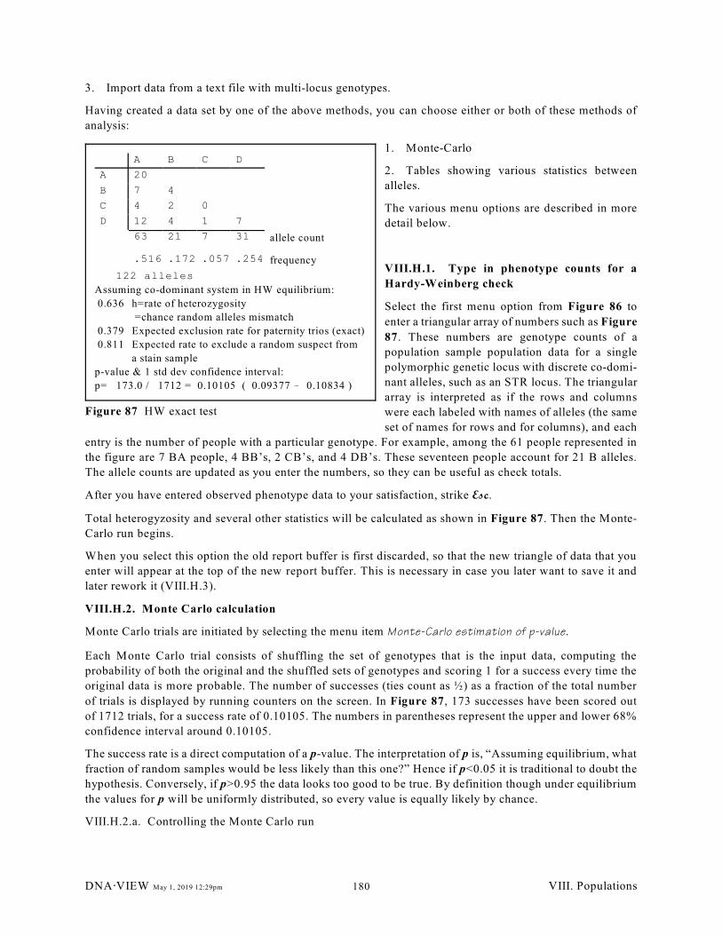
A B C D
A 20
B 7 4
C 4 2 0
D 12 4 1 7
63 21 7 31 allele count
.516 .172 .057 .254 frequency
122 alleles
Assuming co-dominant system in HW equilibrium:
0.636 h=rate of heterozygosity
=chance random alleles mismatch
0.379 Expected exclusion rate for paternity trios (exact)
0.811 Expected rate to exclude a random suspect from
a stain sample
p-value & 1 std dev confidence interval:
p= 173.0 / 1712 = 0.10105 ( 0.09377 ! 0.10834 )
Figure 87 HW exact test
3. Import data from a text file with multi-locus genotypes.
Having created a data set by one of the above methods, you can choose either or both of these methods of
analysis:
1. Monte-Carlo
2. Tables showing various statistics between
alleles.
The various menu options are described in more
detail below.
VIII.H.1. Type in phenotype counts for a
Hardy-Weinberg check
Select the first menu option from Figure 86 to
enter a triangular array of numbers such as Figure
87. These numbers are genotype counts of a
population sample population data for a single
polymorphic genetic locus with discrete co-domi-
nant alleles, such as an STR locus. The triangular
array is interpreted as if the rows and columns
were each labeled with names of alleles (the same
set of names for rows and for columns), and each
entry is the number of people with a particular genotype. For example, among the 61 people represented in
the figure are 7 BA people, 4 BB’s, 2 CB’s, and 4 DB’s. These seventeen people account for 21 B alleles.
The allele counts are updated as you enter the numbers, so they can be useful as check totals.
After you have entered observed phenotype data to your satisfaction, strike Esc.
Total heterogyzosity and several other statistics will be calculated as shown in Figure 87. Then the Monte-
Carlo run begins.
When you select this option the old report buffer is first discarded, so that the new triangle of data that you
enter will appear at the top of the new report buffer. This is necessary in case you later want to save it and
later rework it (VIII.H.3).
VIII.H.2. Monte Carlo calculation
Monte Carlo trials are initiated by selecting the menu item Monte-Carlo estimation of p-value.
Each Monte Carlo trial consists of shuffling the set of genotypes that is the input data, computing the
probability of both the original and the shuffled sets of genotypes and scoring 1 for a success every time the
original data is more probable. The number of successes (ties count as ½) as a fraction of the total number
of trials is displayed by running counters on the screen. In Figure 87, 173 successes have been scored out
of 1712 trials, for a success rate of 0.10105. The numbers in parentheses represent the upper and lower 68%
confidence interval around 0.10105.
The success rate is a direct computation of a p-value. The interpretation of p is, “Assuming equilibrium, what
fraction of random samples would be less likely than this one?” Hence if p<0.05 it is traditional to doubt the
hypothesis. Conversely, if p>0.95 the data looks too good to be true. By definition though under equilibrium
the values for p will be uniformly distributed, so every value is equally likely by chance.
VIII.H.2.a. Controlling the Monte Carlo run
DNA@VIEW May 1, 2019 12:29pm VIII. Populations180
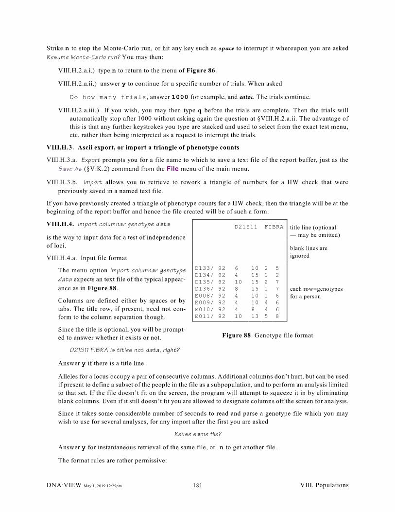
D21S11 FIBRA title line (optional
— may be omitted)
blank lines are
ignored
D133/ 92D134/ 92D135/ 92D136/ 92E008/ 92E009/ 92E010/ 92E011/ 92
6410844410
101515151010813
21211445
52776668
each row=genotypes
for a person
Figure 88 Genotype file format
Strike n to stop the Monte-Carlo run, or hit any key such as space to interrupt it whereupon you are asked
Resume Monte-Carlo run? You may then:
VIII.H.2.a.i.) type n to return to the menu of Figure 86.
VIII.H.2.a.ii.) answer y to continue for a specific number of trials. When asked
Do how many trials, answer 1000 for example, and enter. The trials continue.
VIII.H.2.a.iii.) If you wish, you may then type q before the trials are complete. Then the trials will
automatically stop after 1000 without asking again the question at §VIII.H.2.a.ii. The advantage of
this is that any further keystrokes you type are stacked and used to select from the exact test menu,
etc, rather than being interpreted as a request to interrupt the trials.
VIII.H.3. Ascii export, or import a triangle of phenotype counts
VIII.H.3.a. Export prompts you for a file name to which to save a text file of the report buffer, just as the
Save As (§V.K.2) command from the File menu of the main menu.
VIII.H.3.b. Import allows you to retrieve to rework a triangle of numbers for a HW check that were
previously saved in a named text file.
If you have previously created a triangle of phenotype counts for a HW check, then the triangle will be at the
beginning of the report buffer and hence the file created will be of such a form.
VIII.H.4. Import columnar genotype data
is the way to input data for a test of independence
of loci.
VIII.H.4.a. Input file format
The menu option Import columnar genotype
data expects an text file of the typical appear-
ance as in Figure 88.
Columns are defined either by spaces or by
tabs. The title row, if present, need not con-
form to the column separation though.
Since the title is optional, you will be prompt-
ed to answer whether it exists or not.
D21S11 FIBRA is titles not data, right?
Answer y if there is a title line.
Alleles for a locus occupy a pair of consecutive columns. Additional columns don’t hurt, but can be used
if present to define a subset of the people in the file as a subpopulation, and to perform an analysis limited
to that set. If the file doesn’t fit on the screen, the program will attempt to squeeze it in by eliminating
blank columns. Even if it still doesn’t fit you are allowed to designate columns off the screen for analysis.
Since it takes some considerable number of seconds to read and parse a genotype file which you may
wish to use for several analyses, for any import after the first you are asked
Reuse same file?
Answer y for instantaneous retrieval of the same file, or n to get another file.
The format rules are rather permissive:
DNA@VIEW May 1, 2019 12:29pm VIII. Populations181
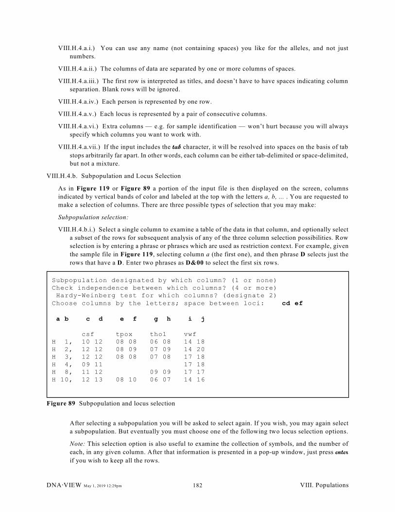
Subpopulation designated by which column? (1 or none)Check independence between which columns? (4 or more) Hardy-Weinberg test for which columns? (designate 2)Choose columns by the letters; space between loci: cd ef
a b c d e f g h i j
csf tpox tho1 vwfH 1, 10 12 08 08 06 08 14 18H 2, 12 12 08 09 07 09 14 20H 3, 12 12 08 08 07 08 17 18H 4, 09 11 17 18H 8, 11 12 09 09 17 17H 10, 12 13 08 10 06 07 14 16
Figure 89 Subpopulation and locus selection
VIII.H.4.a.i.) You can use any name (not containing spaces) you like for the alleles, and not just
numbers.
VIII.H.4.a.ii.) The columns of data are separated by one or more columns of spaces.
VIII.H.4.a.iii.) The first row is interpreted as titles, and doesn’t have to have spaces indicating column
separation. Blank rows will be ignored.
VIII.H.4.a.iv.) Each person is represented by one row.
VIII.H.4.a.v.) Each locus is represented by a pair of consecutive columns.
VIII.H.4.a.vi.) Extra columns — e.g. for sample identification — won’t hurt because you will always
specify which columns you want to work with.
VIII.H.4.a.vii.) If the input includes the tab character, it will be resolved into spaces on the basis of tab
stops arbitrarily far apart. In other words, each column can be either tab-delimited or space-delimited,
but not a mixture.
VIII.H.4.b. Subpopulation and Locus Selection
As in Figure 119 or Figure 89 a portion of the input file is then displayed on the screen, columns
indicated by vertical bands of color and labeled at the top with the letters a, b, ... . You are requested to
make a selection of columns. There are three possible types of selection that you may make:
Subpopulation selection:
VIII.H.4.b.i.) Select a single column to examine a table of the data in that column, and optionally select
a subset of the rows for subsequent analysis of any of the three column selection possibilities. Row
selection is by entering a phrase or phrases which are used as restriction context. For example, given
the sample file in Figure 119, selecting column a (the first one), and then phrase D selects just the
rows that have a D. Enter two phrases as D&00 to select the first six rows.
After selecting a subpopulation you will be asked to select again. If you wish, you may again select
a subpopulation. But eventually you must choose one of the following two locus selection options.
Note: This selection option is also useful to examine the collection of symbols, and the number of
each, in any given column. After that information is presented in a pop-up window, just press enter
if you wish to keep all the rows.
DNA@VIEW May 1, 2019 12:29pm VIII. Populations182
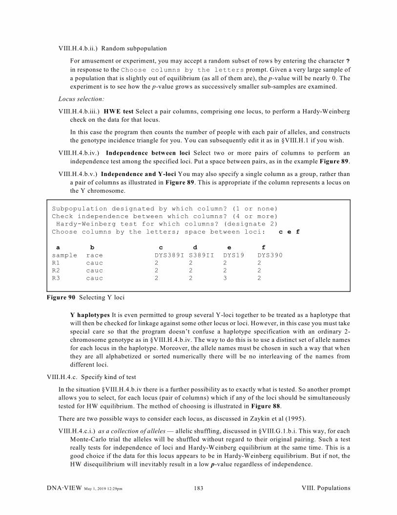
Subpopulation designated by which column? (1 or none)Check independence between which columns? (4 or more) Hardy-Weinberg test for which columns? (designate 2)Choose columns by the letters; space between loci: c e f
a b c d e fsample race DYS389I S389II DYS19 DYS390R1 cauc 2 2 2 2R2 cauc 2 2 2 2R3 cauc 2 2 3 2
Figure 90 Selecting Y loci
VIII.H.4.b.ii.) Random subpopulation
For amusement or experiment, you may accept a random subset of rows by entering the character ?
in response to the Choose columns by the letters prompt. Given a very large sample of
a population that is slightly out of equilibrium (as all of them are), the p-value will be nearly 0. The
experiment is to see how the p-value grows as successively smaller sub-samples are examined.
Locus selection:
VIII.H.4.b.iii.) HWE test Select a pair columns, comprising one locus, to perform a Hardy-Weinberg
check on the data for that locus.
In this case the program then counts the number of people with each pair of alleles, and constructs
the genotype incidence triangle for you. You can subsequently edit it as in §VIII.H.1 if you wish.
VIII.H.4.b.iv.) Independence between loci Select two or more pairs of columns to perform an
independence test among the specified loci. Put a space between pairs, as in the example Figure 89.
VIII.H.4.b.v.) Independence and Y-loci You may also specify a single column as a group, rather than
a pair of columns as illustrated in Figure 89. This is appropriate if the column represents a locus on
the Y chromosome.
Y haplotypes It is even permitted to group several Y-loci together to be treated as a haplotype that
will then be checked for linkage against some other locus or loci. However, in this case you must take
special care so that the program doesn’t confuse a haplotype specification with an ordinary 2-
chromosome genotype as in §VIII.H.4.b.iv. The way to do this is to use a distinct set of allele names
for each locus in the haplotype. Moreover, the allele names must be chosen in such a way that when
they are all alphabetized or sorted numerically there will be no interleaving of the names from
different loci.
VIII.H.4.c. Specify kind of test
In the situation §VIII.H.4.b.iv there is a further possibility as to exactly what is tested. So another prompt
allows you to select, for each locus (pair of columns) which if any of the loci should be simultaneously
tested for HW equilibrium. The method of choosing is illustrated in Figure 88.
There are two possible ways to consider each locus, as discussed in Zaykin et al (1995).
VIII.H.4.c.i.) as a collection of alleles — allelic shuffling, discussed in §VIII.G.1.b.i. This way, for each
Monte-Carlo trial the alleles will be shuffled without regard to their original pairing. Such a test
really tests for independence of loci and Hardy-Weinberg equilibrium at the same time. This is a
good choice if the data for this locus appears to be in Hardy-Weinberg equilibrium. But if not, the
HW disequilibrium will inevitably result in a low p-value regardless of independence.
DNA@VIEW May 1, 2019 12:29pm VIII. Populations183
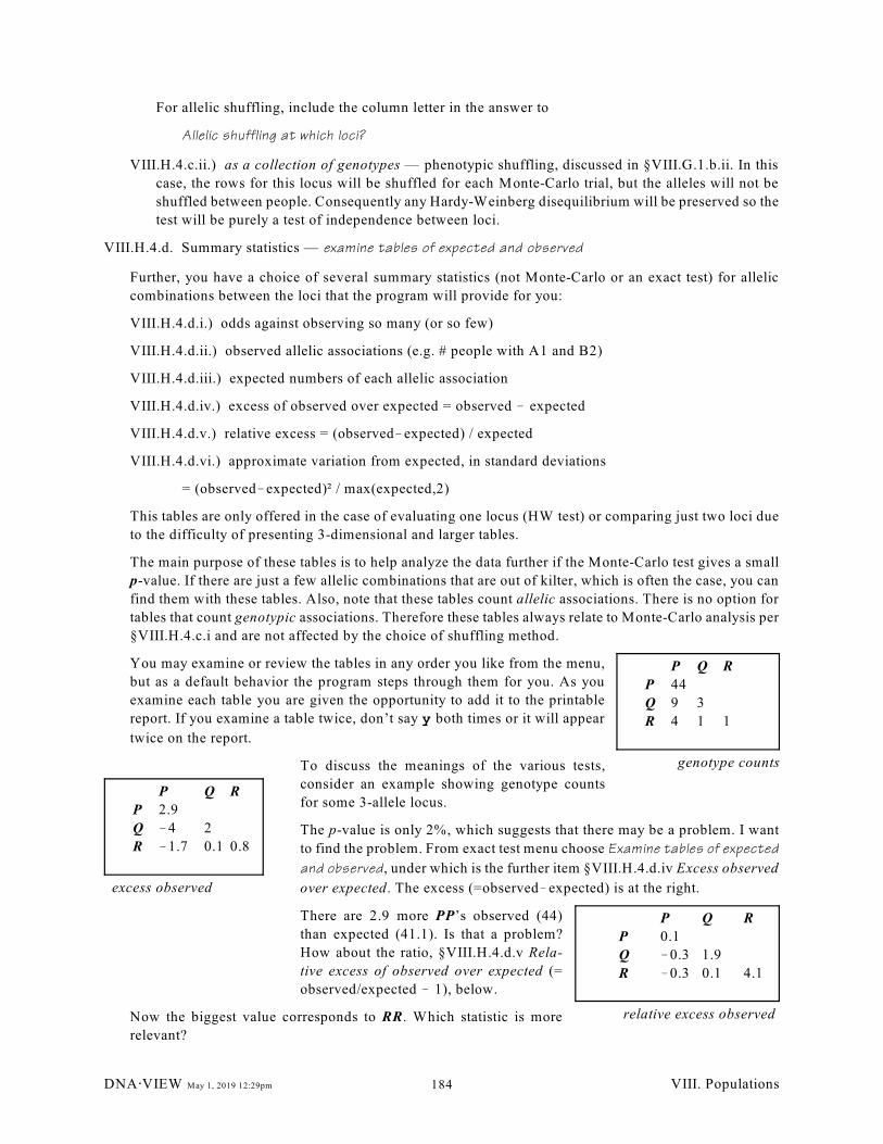
P Q R
P 44
Q 9 3
R 4 1 1
genotype counts
P Q R
P 2.9
Q !4 2
R !1.7 0.1 0.8
excess observed
P Q R
P 0.1
Q !0.3 1.9
R !0.3 0.1 4.1
relative excess observed
For allelic shuffling, include the column letter in the answer to
Allelic shuffling at which loci?
VIII.H.4.c.ii.) as a collection of genotypes — phenotypic shuffling, discussed in §VIII.G.1.b.ii. In this
case, the rows for this locus will be shuffled for each Monte-Carlo trial, but the alleles will not be
shuffled between people. Consequently any Hardy-Weinberg disequilibrium will be preserved so the
test will be purely a test of independence between loci.
VIII.H.4.d. Summary statistics — examine tables of expected and observed
Further, you have a choice of several summary statistics (not Monte-Carlo or an exact test) for allelic
combinations between the loci that the program will provide for you:
VIII.H.4.d.i.) odds against observing so many (or so few)
VIII.H.4.d.ii.) observed allelic associations (e.g. # people with A1 and B2)
VIII.H.4.d.iii.) expected numbers of each allelic association
VIII.H.4.d.iv.) excess of observed over expected = observed ! expected
VIII.H.4.d.v.) relative excess = (observed!expected) / expected
VIII.H.4.d.vi.) approximate variation from expected, in standard deviations
= (observed!expected)² / max(expected,2)
This tables are only offered in the case of evaluating one locus (HW test) or comparing just two loci due
to the difficulty of presenting 3-dimensional and larger tables.
The main purpose of these tables is to help analyze the data further if the Monte-Carlo test gives a small
p-value. If there are just a few allelic combinations that are out of kilter, which is often the case, you can
find them with these tables. Also, note that these tables count allelic associations. There is no option for
tables that count genotypic associations. Therefore these tables always relate to Monte-Carlo analysis per
§VIII.H.4.c.i and are not affected by the choice of shuffling method.
You may examine or review the tables in any order you like from the menu,
but as a default behavior the program steps through them for you. As you
examine each table you are given the opportunity to add it to the printable
report. If you examine a table twice, don’t say y both times or it will appear
twice on the report.
To discuss the meanings of the various tests,
consider an example showing genotype counts
for some 3-allele locus.
The p-value is only 2%, which suggests that there may be a problem. I want
to find the problem. From exact test menu choose Examine tables of expected
and observed, under which is the further item §VIII.H.4.d.iv Excess observed
over expected. The excess (=observed!expected) is at the right.
There are 2.9 more PP’s observed (44)
than expected (41.1). Is that a problem?
How about the ratio, §VIII.H.4.d.v Rela-
tive excess of observed over expected (=
observed/expected ! 1), below.
Now the biggest value corresponds to RR. Which statistic is more
relevant?
DNA@VIEW May 1, 2019 12:29pm VIII. Populations184
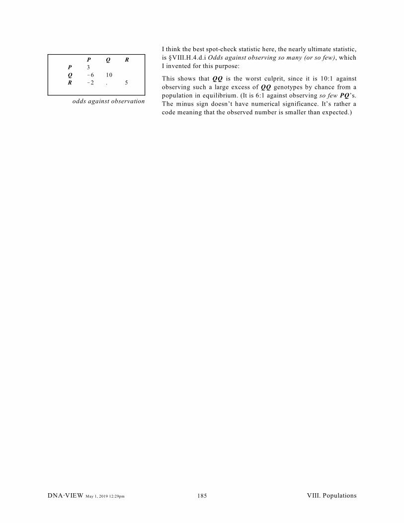
P Q R
P 3
Q !6 10
R !2 . 5
odds against observation
I think the best spot-check statistic here, the nearly ultimate statistic,
is §VIII.H.4.d.i Odds against observing so many (or so few), which
I invented for this purpose:
This shows that QQ is the worst culprit, since it is 10:1 against
observing such a large excess of QQ genotypes by chance from a
population in equilibrium. (It is 6:1 against observing so few PQ’s.
The minus sign doesn’t have numerical significance. It’s rather a
code meaning that the observed number is smaller than expected.)
DNA@VIEW May 1, 2019 12:29pm VIII. Populations185
VIII.I. Database similarity test
Use: “Validate” a database.
A reasonable assessment of database validity for a known population is by comparison with another sample
from the same population.
This command implements an extension that I developed of Fisher’s (original) exact test. Weir (1996 –
Genetic Data Analysis II) discusses the use of Fisher’s test to compare several population samples for the
same locus and (ostensibly) the same race. The result of the test is a p-value that represents the chance that
such differences as there are would occur by chance if in fact the null hypothesis – the hypothesis that all
samples are drawn randomly from the same population – is true. Otherwise put, if the p-value is very low,
that indicates statistically significant variations in allele frequencies – different populations.
My generalization is to permit simultaneous evaluations of several loci, with only a single p-value
representing the result of all comparisons. I am not aware of a publication discussing this particular extension,
but it is a straightforward probability test.
The raft of papers that pretend to validate databases (genotype population samples) by testing for Hardy-
Weinberg equilibrium (§VIII.G) could be improved by using this test instead. At least it says something
meaningful.
VIII.I.1. Outline of use
You have databases for some population for multiple loci, and “reference” databases for the same loci from
previous population studies. The reference databases need not be the same for each locus but usually they will
be.
The ultimate goal is single statistic (§VIII.I.2.b) which says whether there is a significant difference among
the various population samples. For example, if the single overall p=0.3, that means that a fat healthy 30%
of the time that the conglomeration of the given samples were re-apportioned at random into separate samples,
the inter-sample differences would be at least as large as the observed differences among the real data. The
implicit conclusion is that since the observed differences would occur quite often by chance, it is believable
that they in fact did occur by chance (i.e. by “sampling variation”).
Sometimes, the single overall p-value does not turn out to be small as hoped, but rather p=0. In that case it
might be interesting to see if some particular locus or loci are mostly responsible – are problem loci. See
§VIII.I.2.d and also §VIII.I.2.c. If the populations are as disparate as different traditional races then probably
p=0 for every locus individually, but for clearly related populations such as Caucasians and Ashkenazy Jews,
or Japanese and Koreans, there may be definite differences but only sporadic ones.
As you proceed with analyses, results of your operations are added to a report which you may afterwards print
etc (§V.K)
VIII.I.2. Operation
The Database similarity test repeatedly offers a menu with a set of options of in order to let you add to,
subtract from, or analyze a collection of databases to compare.
VIII.I.2.a. Add a set of databases for another locus
This option is automatically “chosen” for you when you begin the analysis.
DNA@VIEW May 1, 2019 12:29pm VIII. Populations186
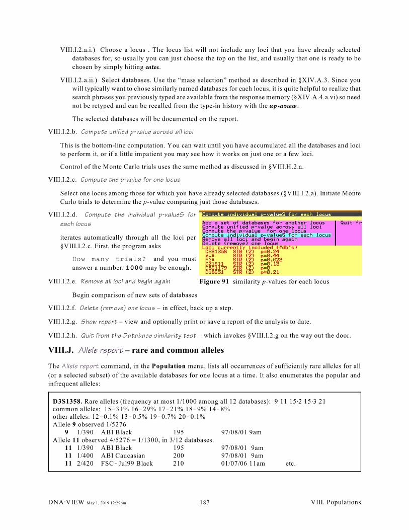
Figure 91 similarity p-values for each locus
D3S1358. Rare alleles (frequency at most 1/1000 among all 12 databases): 9 11 15@2 15@3 21common alleles: 15!31% 16!29% 17!21% 18!9% 14!8%other alleles: 12!0.1% 13!0.5% 19!0.7% 20!0.1%Allele 9 observed 1/5276
9 1/390 ABI Black 195 97/08/01 9amAllele 11 observed 4/5276 = 1/1300, in 3/12 databases.
11 1/390 ABI Black 195 97/08/01 9am11 1/400 ABI Caucasian 200 97/08/01 9am11 2/420 FSC!Jul99 Black 210 01/07/06 11am etc.
VIII.I.2.a.i.) Choose a locus . The locus list will not include any loci that you have already selected
databases for, so usually you can just choose the top on the list, and usually that one is ready to be
chosen by simply hitting enter.
VIII.I.2.a.ii.) Select databases. Use the “mass selection” method as described in §XIV.A.3. Since you
will typically want to chose similarly named databases for each locus, it is quite helpful to realize that
search phrases you previously typed are available from the response memory (§XIV.A.4.a.vi) so need
not be retyped and can be recalled from the type-in history with the up-arrow.
The selected databases will be documented on the report.
VIII.I.2.b. Compute unified p-value across all loci
This is the bottom-line computation. You can wait until you have accumulated all the databases and loci
to perform it, or if a little impatient you may see how it works on just one or a few loci.
Control of the Monte Carlo trials uses the same method as discussed in §VIII.H.2.a.
VIII.I.2.c. Compute the p-value for one locus
Select one locus among those for which you have already selected databases (§VIII.I.2.a). Initiate Monte
Carlo trials to determine the p-value comparing just those databases.
VIII.I.2.d. Compute the individual p-valueS for
each locus
iterates automatically through all the loci per
§VIII.I.2.c. First, the program asks
How many trials? and you must
answer a number. 1000 may be enough.
VIII.I.2.e. Remove all loci and begin again
Begin comparison of new sets of databases
VIII.I.2.f. Delete (remove) one locus – in effect, back up a step.
VIII.I.2.g. Show report – view and optionally print or save a report of the analysis to date.
VIII.I.2.h. Quit from the Database similarity test – which invokes §VIII.I.2.g on the way out the door.
VIII.J. Allele report – rare and common alleles
The Allele report command, in the Population menu, lists all occurrences of sufficiently rare alleles for all
(or a selected subset) of the available databases for one locus at a time. It also enumerates the popular and
infrequent alleles:
DNA@VIEW May 1, 2019 12:29pm VIII. Populations187

DNA@VIEW May 1, 2019 12:29pm VIII. Populations188
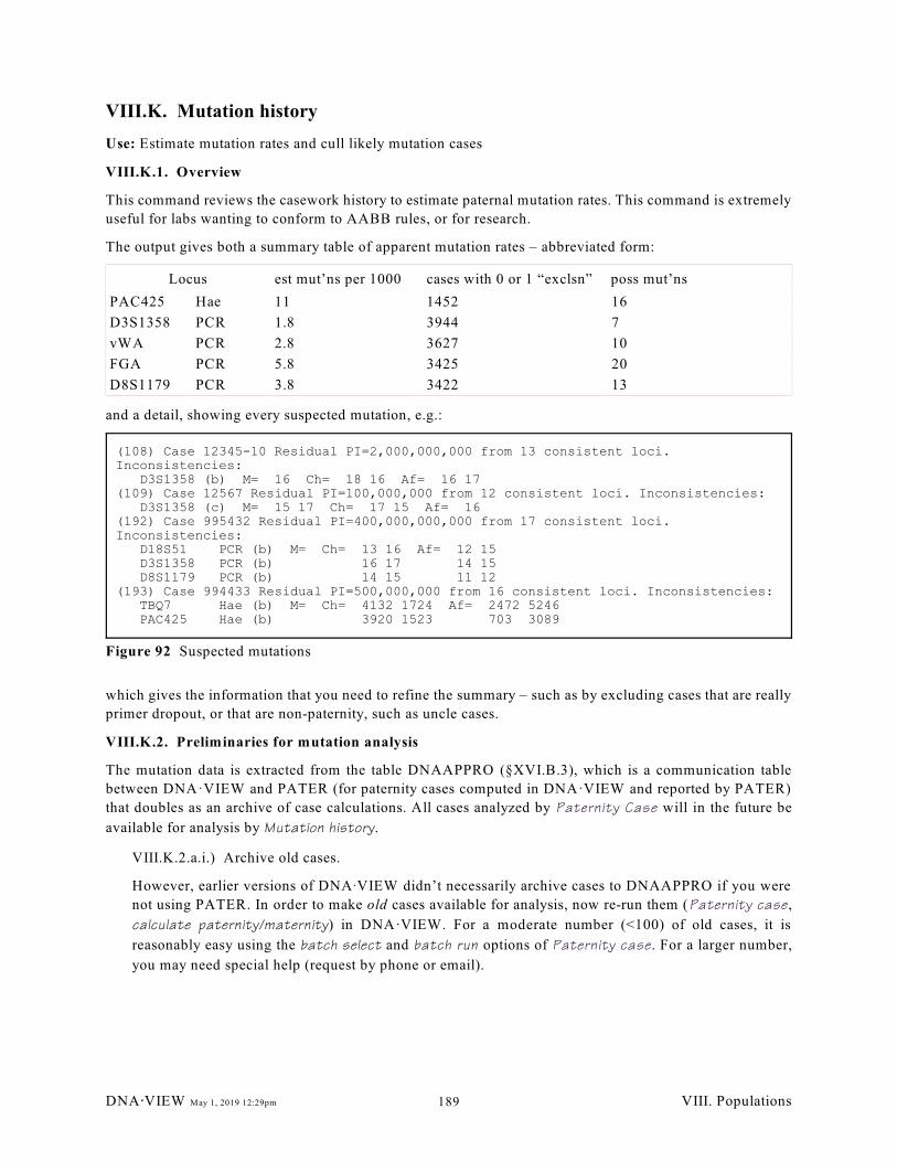
(108) Case 12345-10 Residual PI=2,000,000,000 from 13 consistent loci.Inconsistencies: D3S1358 (b) M= 16 Ch= 18 16 Af= 16 17(109) Case 12567 Residual PI=100,000,000 from 12 consistent loci. Inconsistencies: D3S1358 (c) M= 15 17 Ch= 17 15 Af= 16(192) Case 995432 Residual PI=400,000,000,000 from 17 consistent loci.Inconsistencies: D18S51 PCR (b) M= Ch= 13 16 Af= 12 15 D3S1358 PCR (b) 16 17 14 15 D8S1179 PCR (b) 14 15 11 12(193) Case 994433 Residual PI=500,000,000 from 16 consistent loci. Inconsistencies: TBQ7 Hae (b) M= Ch= 4132 1724 Af= 2472 5246 PAC425 Hae (b) 3920 1523 703 3089
Figure 92 Suspected mutations
VIII.K. Mutation history
Use: Estimate mutation rates and cull likely mutation cases
VIII.K.1. Overview
This command reviews the casework history to estimate paternal mutation rates. This command is extremely
useful for labs wanting to conform to AABB rules, or for research.
The output gives both a summary table of apparent mutation rates – abbreviated form:
Locus est mut’ns per 1000 cases with 0 or 1 “exclsn” poss mut’ns
PAC425 Hae 11 1452 16
D3S1358 PCR 1.8 3944 7
vWA PCR 2.8 3627 10
FGA PCR 5.8 3425 20
D8S1179 PCR 3.8 3422 13
and a detail, showing every suspected mutation, e.g.:
which gives the information that you need to refine the summary – such as by excluding cases that are really
primer dropout, or that are non-paternity, such as uncle cases.
VIII.K.2. Preliminaries for mutation analysis
The mutation data is extracted from the table DNAAPPRO (§XVI.B.3), which is a communication table
between DNA·VIEW and PATER (for paternity cases computed in DNA·VIEW and reported by PATER)
that doubles as an archive of case calculations. All cases analyzed by Paternity Case will in the future be
available for analysis by Mutation history.
VIII.K.2.a.i.) Archive old cases.
However, earlier versions of DNAAVIEW didn’t necessarily archive cases to DNAAPPRO if you were
not using PATER. In order to make old cases available for analysis, now re-run them (Paternity case,
calculate paternity/maternity) in DNA·VIEW. For a moderate number (<100) of old cases, it is
reasonably easy using the batch select and batch run options of Paternity case. For a larger number,
you may need special help (request by phone or email).
DNA@VIEW May 1, 2019 12:29pm VIII. Populations189
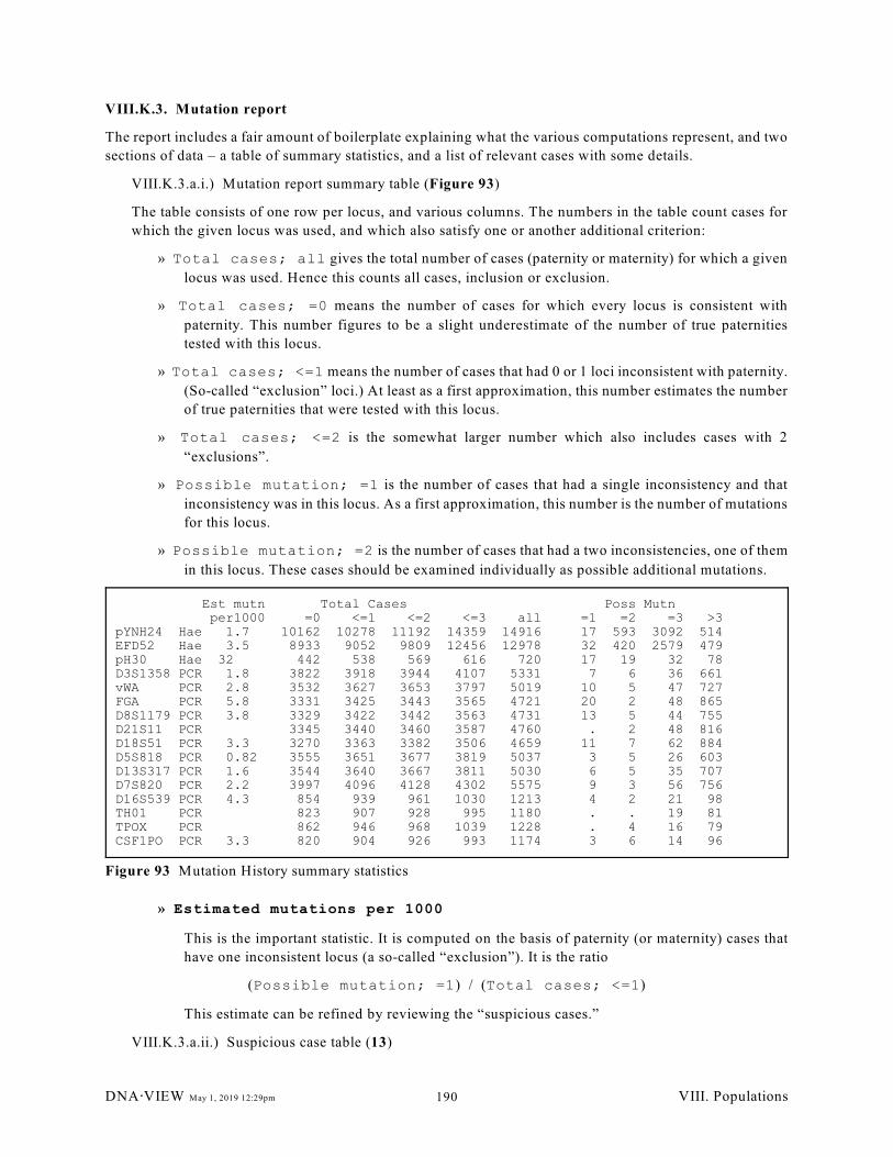
Est mutn Total Cases Poss Mutn per1000 =0 <=1 <=2 <=3 all =1 =2 =3 >3pYNH24 Hae 1.7 10162 10278 11192 14359 14916 17 593 3092 514EFD52 Hae 3.5 8933 9052 9809 12456 12978 32 420 2579 479pH30 Hae 32 442 538 569 616 720 17 19 32 78D3S1358 PCR 1.8 3822 3918 3944 4107 5331 7 6 36 661vWA PCR 2.8 3532 3627 3653 3797 5019 10 5 47 727FGA PCR 5.8 3331 3425 3443 3565 4721 20 2 48 865D8S1179 PCR 3.8 3329 3422 3442 3563 4731 13 5 44 755D21S11 PCR 3345 3440 3460 3587 4760 . 2 48 816D18S51 PCR 3.3 3270 3363 3382 3506 4659 11 7 62 884D5S818 PCR 0.82 3555 3651 3677 3819 5037 3 5 26 603D13S317 PCR 1.6 3544 3640 3667 3811 5030 6 5 35 707D7S820 PCR 2.2 3997 4096 4128 4302 5575 9 3 56 756D16S539 PCR 4.3 854 939 961 1030 1213 4 2 21 98TH01 PCR 823 907 928 995 1180 . . 19 81TPOX PCR 862 946 968 1039 1228 . 4 16 79CSF1PO PCR 3.3 820 904 926 993 1174 3 6 14 96
Figure 93 Mutation History summary statistics
VIII.K.3. Mutation report
The report includes a fair amount of boilerplate explaining what the various computations represent, and two
sections of data – a table of summary statistics, and a list of relevant cases with some details.
VIII.K.3.a.i.) Mutation report summary table (Figure 93)
The table consists of one row per locus, and various columns. The numbers in the table count cases for
which the given locus was used, and which also satisfy one or another additional criterion:
» Total cases; all gives the total number of cases (paternity or maternity) for which a given
locus was used. Hence this counts all cases, inclusion or exclusion.
» Total cases; =0 means the number of cases for which every locus is consistent with
paternity. This number figures to be a slight underestimate of the number of true paternities
tested with this locus.
» Total cases; <=1 means the number of cases that had 0 or 1 loci inconsistent with paternity.
(So-called “exclusion” loci.) At least as a first approximation, this number estimates the number
of true paternities that were tested with this locus.
» Total cases; <=2 is the somewhat larger number which also includes cases with 2
“exclusions”.
» Possible mutation; =1 is the number of cases that had a single inconsistency and that
inconsistency was in this locus. As a first approximation, this number is the number of mutations
for this locus.
» Possible mutation; =2 is the number of cases that had a two inconsistencies, one of them
in this locus. These cases should be examined individually as possible additional mutations.
» Estimated mutations per 1000
This is the important statistic. It is computed on the basis of paternity (or maternity) cases that
have one inconsistent locus (a so-called “exclusion”). It is the ratio
(Possible mutation; =1) / (Total cases; <=1)
This estimate can be refined by reviewing the “suspicious cases.”
VIII.K.3.a.ii.) Suspicious case table (13)
DNA@VIEW May 1, 2019 12:29pm VIII. Populations190
All suspected mutations are listed. Cases are included if
» there were exactly 1 or 2 or 3 inconsistent loci, and
» the residual PI>100.
Only the inconsistent loci are shown. Grossly illegal data (base pairs<0) are removed first. However,
some PCR types may be shown as a ?. If so, then the locus is re-listed ("again:") with the base pair sizes.
Review the instances of possible mutation. This table is intended to be useful for sorting them out, but
obviously the best determination requires researching other records and finally, making some sort of
judgement.
DNA@VIEW May 1, 2019 12:29pm VIII. Populations191
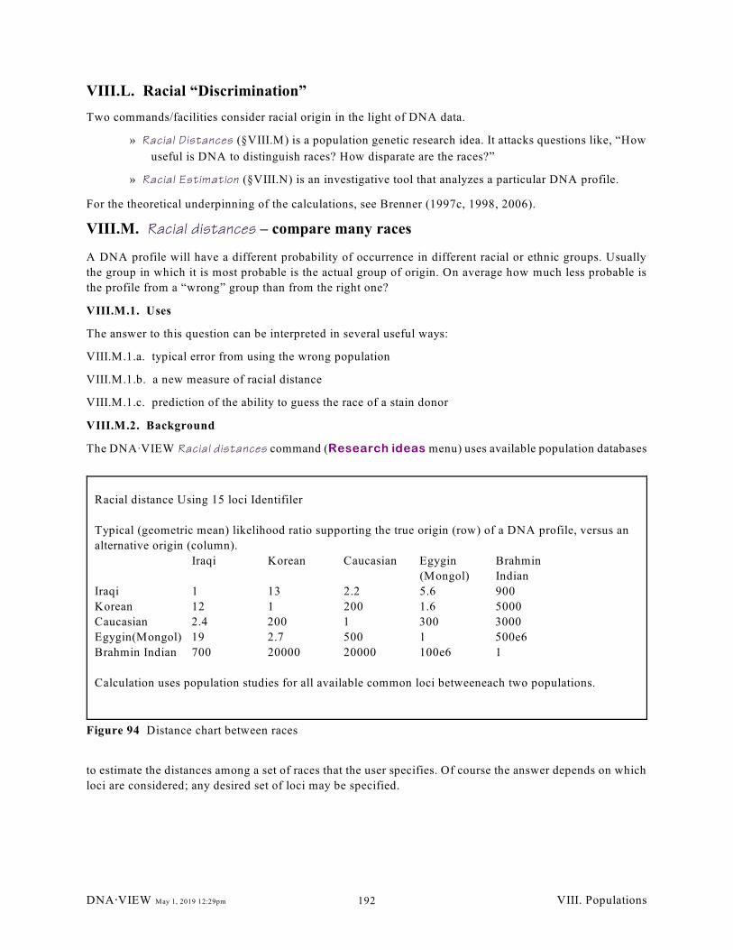
Racial distance Using 15 loci Identifiler
Typical (geometric mean) likelihood ratio supporting the true origin (row) of a DNA profile, versus an
alternative origin (column).
Iraqi Korean Caucasian Egygin
(Mongol)
Brahmin
Indian
Iraqi 1 13 2.2 5.6 900
Korean 12 1 200 1.6 5000
Caucasian 2.4 200 1 300 3000
Egygin(Mongol) 19 2.7 500 1 500e6
Brahmin Indian 700 20000 20000 100e6 1
Calculation uses population studies for all available common loci betweeneach two populations.
Figure 94 Distance chart between races
VIII.L. Racial “Discrimination”
Two commands/facilities consider racial origin in the light of DNA data.
» Racial Distances (§VIII.M) is a population genetic research idea. It attacks questions like, “How
useful is DNA to distinguish races? How disparate are the races?”
» Racial Estimation (§VIII.N) is an investigative tool that analyzes a particular DNA profile.
For the theoretical underpinning of the calculations, see Brenner (1997c, 1998, 2006).
VIII.M. Racial distances – compare many races
A DNA profile will have a different probability of occurrence in different racial or ethnic groups. Usually
the group in which it is most probable is the actual group of origin. On average how much less probable is
the profile from a “wrong” group than from the right one?
VIII.M.1. Uses
The answer to this question can be interpreted in several useful ways:
VIII.M.1.a. typical error from using the wrong population
VIII.M.1.b. a new measure of racial distance
VIII.M.1.c. prediction of the ability to guess the race of a stain donor
VIII.M.2. Background
The DNAAVIEW Racial distances command (Research ideas menu) uses available population databases
to estimate the distances among a set of races that the user specifies. Of course the answer depends on which
loci are considered; any desired set of loci may be specified.
DNA@VIEW May 1, 2019 12:29pm VIII. Populations192
VIII.M.3. Operation
VIII.M.3.a. Choose the loci to consider
You are first offered the “multiplex” menu (§IX.B.7) in order to select a set of loci. Note that selecting
a single locus is among the possible choices.
VIII.M.3.b. First selection races to compare
From the chart, which shows all the races for which data on some of the selected loci is available (the
number in parentheses is the number of available loci), choose any set of races by typing the race letters.
To consider all the mentioned races, just enter.
VIII.M.3.c. All pair-wise racial distance are then calculated using the formulas described in Brenner (1997c)
and (1998). Where fewer than the maximum number of loci are available for a comparisons between two
loci, the distance determined is scaled up so that all numbers in the table are approximately comparable.
VIII.M.3.d. The result report is displayed on the screen and may be printed (via Print).
VIII.N. Racial estimation
improved The Racial estimation command (in the Casework menu) computes the likelihood to see a given
DNA profiles in each of several races. Comparing these likelihoods gives the likelihood ratios supporting
each race compared to the others. Also, the command permits calculating all the profiles of a case at once,
rather than just one individual. The command is also available in the Immigration/Kinship menu.
VIII.N.1. Initiate operation
VIII.N.1.a. (as a main menu command)
VIII.N.1.a.i.) Choose Casework < Racial estimation .
VIII.N.1.a.ii.) What collection of people? (Person/Case/Worklist) Case
VIII.N.1.a.iii.) Enter a case number or person number, or select a worklist as the case may be
VIII.N.1.b. (as an Immigration/Kinship option)
VIII.N.1.b.i.) Choose Casework < Automatic Kinship (or other Case command).
VIII.N.1.b.ii.) Select case – choose the case
VIII.N.1.b.iii.) Choose Immigration/Kinship < Racial Estimate
VIII.N.2. Tentatively choose races to compare
A chart lists all races for which allele frequency databases are defined as defaults for at least part of the
profile(s). The numbers in parentheses are the numbers of loci for which default databases are specified for
a given race. The suggested default response is a list of those race letters for which nearly complete
(according to a heuristic measure) data is available. Races of possible interest? cEkqR
VIII.N.2.a. database "availability"
For purposes of the Racial estimate command, the databases that are considered are those that are mark-
ed as "default" (§VIII.C.2.b, database, per race).
VIII.N.2.b. Choose any selection of races.
Type in the race letters of interest then enter, or just enter to accept the suggested list.
DNA@VIEW May 1, 2019 12:29pm VIII. Populations193
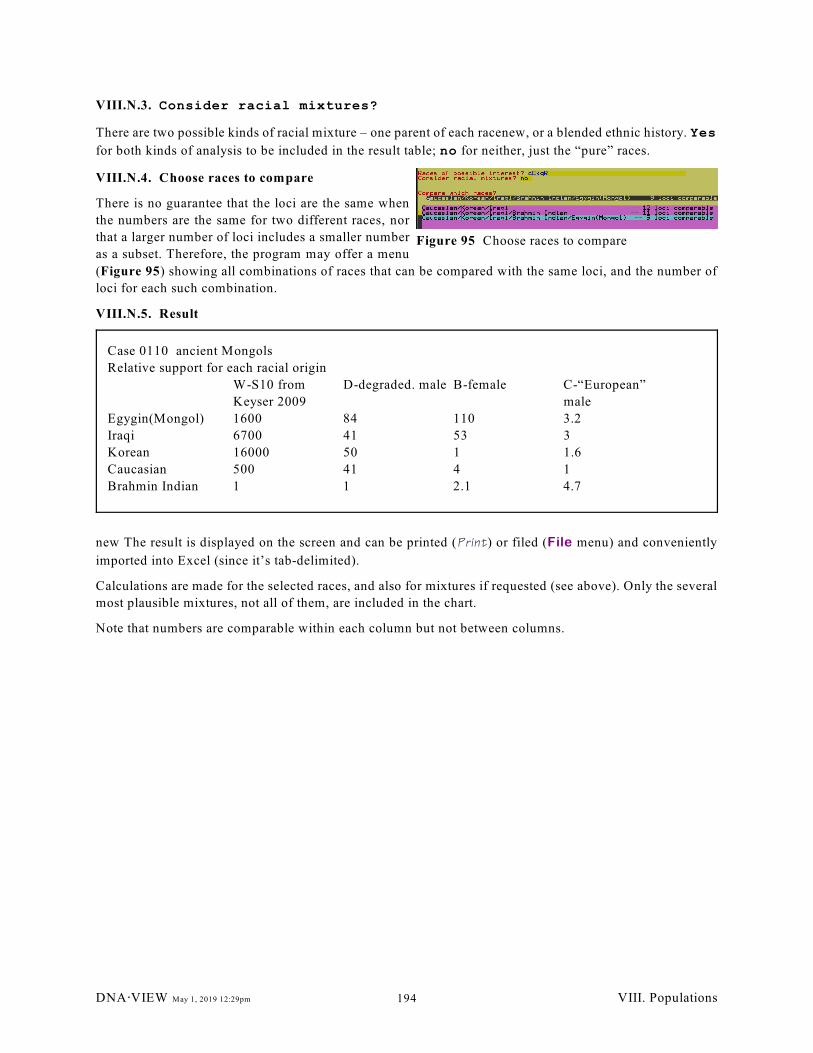
Figure 95 Choose races to compare
Case 0110 ancient Mongols
Relative support for each racial origin
W-S10 from
Keyser 2009
D-degraded. male B-female C-“European”
male
Egygin(Mongol) 1600 84 110 3.2
Iraqi 6700 41 53 3
Korean 16000 50 1 1.6
Caucasian 500 41 4 1
Brahmin Indian 1 1 2.1 4.7
VIII.N.3. Consider racial mixtures?
There are two possible kinds of racial mixture – one parent of each racenew, or a blended ethnic history. Yes
for both kinds of analysis to be included in the result table; no for neither, just the “pure” races.
VIII.N.4. Choose races to compare
There is no guarantee that the loci are the same when
the numbers are the same for two different races, nor
that a larger number of loci includes a smaller number
as a subset. Therefore, the program may offer a menu
(Figure 95) showing all combinations of races that can be compared with the same loci, and the number of
loci for each such combination.
VIII.N.5. Result
new The result is displayed on the screen and can be printed (Print) or filed (File menu) and conveniently
imported into Excel (since it’s tab-delimited).
Calculations are made for the selected races, and also for mixtures if requested (see above). Only the several
most plausible mixtures, not all of them, are included in the chart.
Note that numbers are comparable within each column but not between columns.
DNA@VIEW May 1, 2019 12:29pm VIII. Populations194
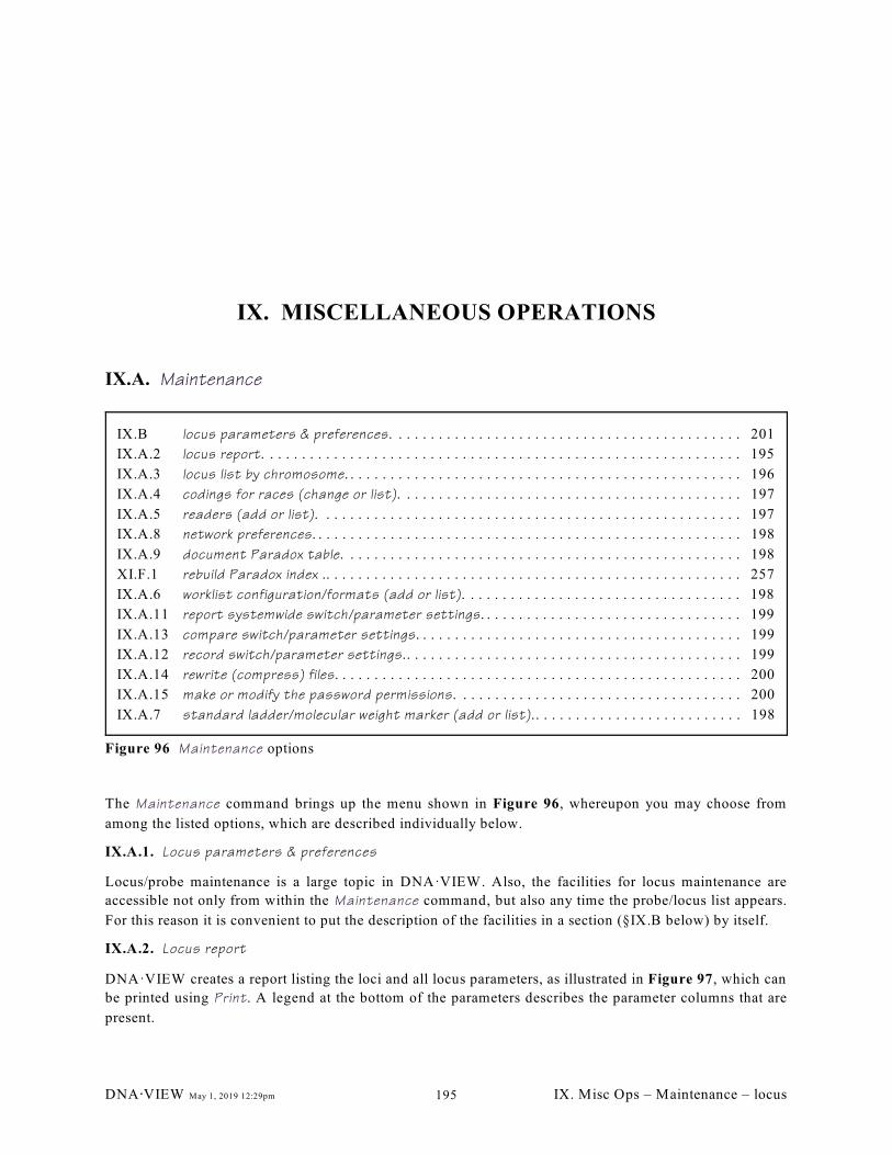
IX.B locus parameters & preferences. . . . . . . . . . . . . . . . . . . . . . . . . . . . . . . . . . . . . . . . . . . . 201
IX.A.2 locus report. . . . . . . . . . . . . . . . . . . . . . . . . . . . . . . . . . . . . . . . . . . . . . . . . . . . . . . . . . . . 195
IX.A.3 locus list by chromosome. . . . . . . . . . . . . . . . . . . . . . . . . . . . . . . . . . . . . . . . . . . . . . . . . . 196
IX.A.4 codings for races (change or list). . . . . . . . . . . . . . . . . . . . . . . . . . . . . . . . . . . . . . . . . . . 197
IX.A.5 readers (add or list). . . . . . . . . . . . . . . . . . . . . . . . . . . . . . . . . . . . . . . . . . . . . . . . . . . . . 197
IX.A.8 network preferences. . . . . . . . . . . . . . . . . . . . . . . . . . . . . . . . . . . . . . . . . . . . . . . . . . . . . . 198
IX.A.9 document Paradox table. . . . . . . . . . . . . . . . . . . . . . . . . . . . . . . . . . . . . . . . . . . . . . . . . . 198
XI.F.1 rebuild Paradox index .. . . . . . . . . . . . . . . . . . . . . . . . . . . . . . . . . . . . . . . . . . . . . . . . . . . . 257
IX.A.6 worklist configuration/formats (add or list). . . . . . . . . . . . . . . . . . . . . . . . . . . . . . . . . . . 198
IX.A.11 report systemwide switch/parameter settings. . . . . . . . . . . . . . . . . . . . . . . . . . . . . . . . . 199
IX.A.13 compare switch/parameter settings. . . . . . . . . . . . . . . . . . . . . . . . . . . . . . . . . . . . . . . . . 199
IX.A.12 record switch/parameter settings.. . . . . . . . . . . . . . . . . . . . . . . . . . . . . . . . . . . . . . . . . . 199
IX.A.14 rewrite (compress) files. . . . . . . . . . . . . . . . . . . . . . . . . . . . . . . . . . . . . . . . . . . . . . . . . . . 200
IX.A.15 make or modify the password permissions. . . . . . . . . . . . . . . . . . . . . . . . . . . . . . . . . . . . 200
IX.A.7 standard ladder/molecular weight marker (add or list).. . . . . . . . . . . . . . . . . . . . . . . . . . 198
Figure 96 Maintenance options
IX. MISCELLANEOUS OPERATIONS
IX.A. Maintenance
The Maintenance command brings up the menu shown in Figure 96, whereupon you may choose from
among the listed options, which are described individually below.
IX.A.1. Locus parameters & preferences
Locus/probe maintenance is a large topic in DNA·VIEW. Also, the facilities for locus maintenance are
accessible not only from within the Maintenance command, but also any time the probe/locus list appears.
For this reason it is convenient to put the description of the facilities in a section (§IX.B below) by itself.
IX.A.2. Locus report
DNA·VIEW creates a report listing the loci and all locus parameters, as illustrated in Figure 97, which can
be printed using Print. A legend at the bottom of the parameters describes the parameter columns that are
present.
DNA@VIEW May 1, 2019 12:29pm IX. Misc Ops – Maintenance – locus195
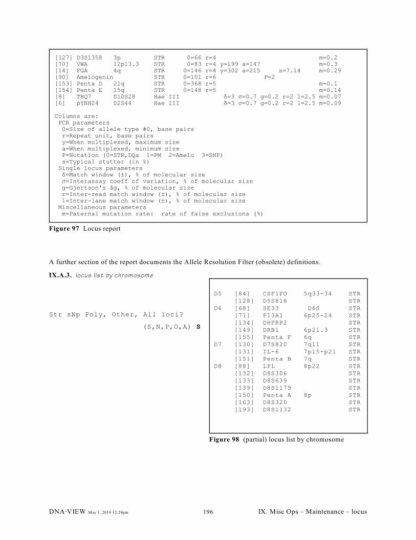
[127] D3S1358 3p STR 0=66 r=4 m=0.2[70] VWA 12p13.3 STR 0=83 r=4 y=199 a=147 m=0.3[14] FGA 4q STR 0=146 r=4 y=302 a=215 s=7.14 m=0.29[90] Amelogenin STR 0=101 r=6 P=2[153] Penta D 21q STR 0=368 r=5 m=0.1[154] Penta E 15q STR 0=148 r=5 m=0.14[8] TBQ7 D10S28 Hae III ä=3 ó=0.7 g=0.2 r=2 l=2.5 m=0.07[6] pYNH24 D2S44 Hae III ä=3 ó=0.7 g=0.2 r=2 l=2.5 m=0.09
Columns are: PCR parameters 0=Size of allele type #0, base pairs r=Repeat unit, base pairs y=When multiplexed, maximum size a=When multiplexed, minimum size P=Notation (0=STR,DQa 1=PM 2=Amelo 3=SNP) s=Typical stutter (in %) Single locus parameters ä=Match window (±), % of molecular size ó=Interassay coeff of variation, % of molecular size g=Gjertson's åg, % of molecular size r=Inter-read match window (±), % of molecular size l=Inter-lane match window (±), % of molecular size Miscellaneous parameters m=Paternal mutation rate: rate of false exclusions (%)
Figure 97 Locus report
D5 [84] CSF1PO 5q33-34 STR [128] D5S818 STRD6 [68] SE33 D6S STR [71] F13A1 6p25-24 STR [134] DHFRP2 STR [149] DRB1 6p21.3 STR [155] Penta F 6q STRD7 [130] D7S820 7q11 STR [131] IL-6 7p15-p21 STR [151] Penta B 7q STRD8 [88] LPL 8p22 STR [132] D8S306 STR [133] D8S639 STR [139] D8S1179 STR [150] Penta A 8p STR [163] D8S320 STR [193] D8S1132 STR
Figure 98 (partial) locus list by chromosome
A further section of the report documents the Allele Resolution Filter (obsolete) definitions.
IX.A.3. locus list by chromosome
Str sNp Poly, Other, All loci?
(S,N,P,O,A) S
DNA@VIEW May 1, 2019 12:29pm IX. Misc Ops – Maintenance – locus196

Figure 99 race codings
IX.A.4. Races
The 52 lower and upper case letters, a-z, A-Z, are used in coding races. You may attach any spelling (i.e. race
name) you like to each one. See Figure 99.
In addition, the dash (–) is used instead of a race letter coding children (since their race is irrelevant for
calculations, and their alleles shouldn’t go into any data base). The dash may also be used to code any other
person who, for whatever reason, will be omitted from all data bases.
§XIV.A.9.a.iii has more information on entering race codes.
IX.A.4.a. race codings (change)
The list of races may be ed-
ited from this Maintenance
option, but it is often more
convenient method to access
the list by answering ? as a
race code any place a race
code is to be supplied —
e.g. from Case or from
Worklist.
To change the race spelling
associated with one of the
race letters:
< From the green menu of
races, put the red bounce bar on the desired item – for example by typing the race letter.
< Select the item by hitting tab (not enter!).
< Type the new name into the answer box, then enter.
IX.A.4.b. race codings (list)
Either by selecting this option, or after using the previous one, a report is prepared listing all the race
codes and their corresponding names. It is available via Print.
IX.A.5. Readers
Some DNAAVIEW operations require the user to select a user identity from the list of readers. Each reader
is a 3-digit number and a name.
Two numbers are special:
» 000 is the “student” user. DNA data provided by user 000 is ignored for computation if other data
(same lane, same locus) is available. However, if the student’s data is the only available data, it
is used.
» 099 is assumed to be a mechanical and hence infallible user. This number can be associated with
data imported from another computer (Genotyper for example). Except for user 099, data that
is entered only once is marked with an asterisk (*) on reports warning that it may be unreliable.
To modify the list of readers,
IX.A.5.a. obtain the list of readers
DNA@VIEW May 1, 2019 12:29pm IX. Misc Ops – Maintenance197
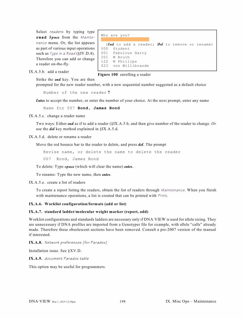
Who are you?
(End to add a reader; Del to remove or rename)000 Student001 Fabulous Harry201 M Bruch122 M Phillips023 von Willibrande
Figure 100 enrolling a reader
Select readers by typing type
read Space from the Mainte-
nance menu. Or, the list appears
as part of various input operations
such as Type in a Read (§IV.D.4).
Therefore you can add or change
a reader on-the-fly.
IX.A.5.b. add a reader
Strike the end key. You are then
prompted for the new reader number, with a new sequential number suggested as a default choice
Number of the new reader 7
Enter to accept the number, or enter the number of your choice. At the next prompt, enter any name
Name for 007 Bond, James Bond
IX.A.5.c. change a reader name
Two ways: Either end as if to add a reader (§IX.A.5.b, and then give number of the reader to change. Or
use the del key method explained in §IX.A.5.d.
IX.A.5.d. delete or rename a reader
Move the red bounce bar to the reader to delete, and press del. The prompt
Revise name, or delete the name to delete the reader
007 Bond, James Bond
To delete: Type space (which will clear the name) enter.
To rename: Type the new name, then enter.
IX.A.5.e. create a list of readers
To create a report listing the readers, obtain the list of readers through Maintenance. When you finish
with maintenance operations, a list is created that can be printed with Print.
IX.A.6. Worklist configuration/formats (add or list)
IX.A.7. standard ladder/molecular weight marker (report, add)
Worklist configurations and standards ladders are necessary only if DNAAVIEW is used for allele sizing. They
are unnecessary if DNA profiles are imported from a Genotyper file for example, with allele “calls” already
made. Therefore these obsolescent sections have been removed. Consult a pre-2007 version of the manual
if interested.
IX.A.8. Network preferences (for Paradox)
Installation issue. See §XV.D.
IX.A.9. document Paradox table
This option may be useful for programmers.
DNA@VIEW May 1, 2019 12:29pm IX. Misc Ops – Maintenance198
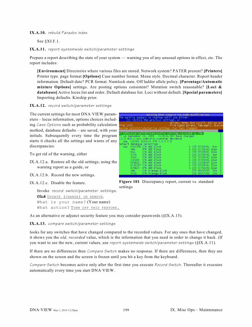
Figure 101 Discrepancy report, current vs. standard
settings
IX.A.10. rebuild Paradox index
See §XI.F.1.
IX.A.11. report systemwide switch/parameter settings
Prepare a report describing the state of your system — warning you of any unusual options in effect, etc. The
report includes:
[Environment] Directories where various files are stored. Network system? PATER present? [Printers]
Printer type. page format [Options] Case number format. Menu style. Decimal character. Report header
information. Default date? PCR format. Numlock state. Off ladder allele policy. [Parentage/Automatic
mixture Options] settings. Are posting options consistent? Mutation switch reasonable? [Loci &
databases] Active locus list and order. Default database list. Loci without default. [Special parameters]
Importing defaults. Kinship prior.
IX.A.12. record switch/parameter settings
The current settings for most DNAAVIEW param-
eters – locus information, options choices includ-
ing Case Options such as probability calculation
method, database defaults – are saved, with your
initials. Subsequently every time the program
starts it checks all the settings and warns of any
discrepancies:
To get rid of the warning, either
IX.A.12.a. Restore all the old settings, using the
warning report as a guide, or
IX.A.12.b. Record the new settings.
IX.A.12.c. Disable the feature.
Invoke record switch/parameter settings.
Click UPDATE (CHANGE) OR REMOVE.
What is your name? (Your name)
What action? TURN OFF THIS FEATURE.
As an alternative or adjunct security feature you may consider passwords (§IX.A.15).
IX.A.13. compare switch/parameter settings
looks for any switches that have changed compared to the recorded values. For any ones that have changed,
it shows you the old, recorded value, which is the information that you need in order to change it back. (If
you want to see the new, current values, use report systemwide switch/parameter settings (§IX.A.11).
If there are no differences then Compare Switch makes no response. If there are differences, then they are
shown on the screen and the screen is frozen until you hit a key from the keyboard.
Compare Switch becomes active only after the first time you execute Record Switch. Thereafter it executes
automatically every time you start DNA@VIEW.
DNA@VIEW May 1, 2019 12:29pm IX. Misc Ops – Maintenance199
IX.A.14. rewrite (compress) files – conserve disk space
Sometimes some DNA·VIEW files accumulate unnecessary dead space. Invoking rewrite files displays a table
of wasted space (“slack”). Select a file from the menu of files and enter to rewrite the file and recover the
space. Or abort (ctrl-C) to do nothing.
Compressing is generally harmless except for the time that may be involved (compressing a 100Mbyte file
on a network might take 5-10 minutes).
Caveat: If you have a networked DNA@VIEW system, every user but one (including PATER users) must sign
off before you use this tool because you can’t compress a file while it is being shared.15
A list is shown of all DNA·VIEW files. For each file, the actual disk space consumed (SIZE) and the amount
of wasted space (SLACK) is shown. The default selection is the one with the largest amount of slack. Select
a file to compress it. You will be asked to wait — even minutes for a file of several megabytes — during the
compression.
Interrupting compression might cause a minor problem. Erasing any files found on the hard disk with the
extension .SFD, such as DNAFREQ.SFD, will cure the problem.
IX.A.15. Password access to critical DNA@VIEW functions
Make or modify the password permissions is an optional security feature to prevent unauthorized changes to
critical DNA@VIEW parameters and settings by requiring a password. Alternatively or in conjuction you can
use the Record switch/parameter settings mechanism (§IX.A.12) which warns if any settings are changed.
The passwords are stored in a special file. If the file has some password records, then various DNA@VIEW
operations require password entry. If the file is empty or non-existent, then password barriers are not used.
There are three security levels.
security level description privilige
1 (highest) supervisor any operation, including delete databases or cases, update to new
DNA@VIEW system, modify locus names, record switch settings
10 user casework, change some locus parameters
20 student casework
The password maintenance screens allow adding or removing passwords, and are self-explanatory.
File #29 is not shared; it is private to each station. So you can compress it anytime.15
DNA@VIEW May 1, 2019 12:29pm IX. Misc Ops – Maintenance200
IX.B. Probe/locus maintenance
DNA@VIEW has hundreds of loci already included including all commonly used forensic loci as of this
writing (Figure 156, Figure 157 and Figure 158, §XVI.A.2). The list is uniform across all users in the sense
that everyone should use the same line numbers — for example, VWA is locus [70]. This is to facilitate
sharing of databases among users. For the same reason, some probes, such as pYNH24, are listed several
times representing the various commonly used restriction enzymes.
At the same time, the list is completely user-maintainable. You can freely change the spelling (e.g. VWF
instead of VWA if you prefer), the values of the various numeric parameters associated with any locus, or
even to add a new locus. However, to maintain world-wide uniformity please check with DNA@VIEW
international headquarters before adding a new locus, and then use the line number that is issued for your
new locus.
Exception: Lines [100]![119] are reserved and available for “Site use” — anything you like, but intended
for usage that you expect will not be of interest to the user community.
Locus maintenance is allowed from every screen that shows the probe/locus list. There are many incidental
situations in which this happens, such as when the user needs to choose a locus to Type in a read.
IX.B.1. Locus maintenance
There are several useful actions to take with the locus list, including selection, reordering, adding, hiding, and
setting properties.
IX.B.1.a. Select a locus
Move the bounce-bar to a locus in the locus list and OK or enter to select the locus.
IX.B.1.b. FULL LIST / SHORT LIST
These buttons toggles between a concise locus list that includes only “active” loci, and an extended list
that includes all loci. The extended list also shows locus number (in the DNA@VIEW list), and a comment
field (not user-changeable) of various information such as alternate names, Genebank information, PCR
parameter possibilities.
If the desired locus is not found in the list, it may be necessary to add it (§IX.B.1.e) but more likely it is
merely hidden (inactive). To check if it is in the list but hidden look at the FULL LIST. Then, because of
the select-context mode of DNAAVIEW menus, typing almost any variation or part of the locus name will
bring it into view.
IX.B.1.c. (DE)ACTIVATE
In order to keep the locus list less cluttered, the (DE)ACTIVATE button lets you hide those majority of
probes/loci that are not of interest. Hidden means the locus is not visible from the SHORT LIST. It is
visible but indented one character on the FULL LIST (§IX.B.1.b).
Activation and deactivation are also possible wholesale using the multiplex mechanism (§IX.B.1.d.i).
IX.B.1.d. Locus ordering – the REORDER buttons
It is convenient to arrange the locus list with commoner loci toward the top, and also to have loci in the
same order as they occur in reference documents. Therefore the user may specify the preferred order of
loci. This order determines:
» the order of loci in the locus list
» the order in which they occur in reports, such as a paternity or kinship calculation
DNA@VIEW May 1, 2019 12:29pm IX. Misc Ops – Locus maintenance201
» the next locus provided as a default suggestion by Database similarity test (§VIII.I.2.a.i) or Type
in a Read (§IV.D.4)
» the next loci introduced by the # key in DNA odds (§V.G), Y haplotype matching LR (§V.H) or
DNA exclusion (§V.I)
There are two methods for ordering loci, wholesale and one-at-a-time.
IX.B.1.d.i.) Wholesale locus ordering
REORDER: MPLX pops up a list of multiplexes (§IX.B.7)
» Select a multiplex from the list and
PUT THESE AT TOP to activate and position the loci of the multiplex in standard order at the top
of the locus list;
ALPHABETIZE AT TOP to activate and position the loci of the multiplex in alphabetized order at
the top of the locus list;
UNORDER to deactivate the loci of the multiplex and move them to the bottom, non-priority part
of the list.
» With no multiplex selected (no bouncebar – try the ___ button), ALPHABETIZE ALL puts all active
loci in alphabetic order.
IX.B.1.d.ii.) Single locus ordering
Highlight a locus and
» 8 and 9 to adjust the position of a locus within the list.
» 99 to remove a locus from the priority list.
IX.B.1.e. Add a locus
It is unlikely that you will need to add a new locus, as all the usual identification loci are already
incorporated in DNA@VIEW. Please see §XVI.A.2. If you don't see a locus that might be expected,
possibly it is present but temporarily hidden.
Therefore, before adding a locus,
IX.B.1.e.i.) Check if the locus is already present, but inactive, per §IX.B.1.b. If it is, you only need to
confirm that the various parameters (i.e. “properties”) are ok (§IX.B.3.f).
IX.B.1.e.ii.) Determine the proper line number for the new locus. See page 313, 314.
IX.B.1.e.iii.) The NEW button opens a dialogue to add a new locus.
Type the line number for the new locus, Enter.
IX.B.1.e.iv.) PROPERTIES (with the new locus line number highlighted) to enter locus maintenance for
the new number at the point of enzyme selection. Select SNP (or PCR, etc) as a pseudo-“enzyme”.
IX.B.1.e.v.) Do each of the relevant maintenance operations, definitely including edit locus name and
assign enzyme.
IX.B.1.e.vi.) Add probe/locus (keystroke instructions)
Here are the steps, keystroke by keystroke, for adding a new PCR locus D17S1290:
Select [Housekeeping], Maintenance from the command menu.
DNA@VIEW May 1, 2019 12:29pm IX. Misc Ops – Locus maintenance202
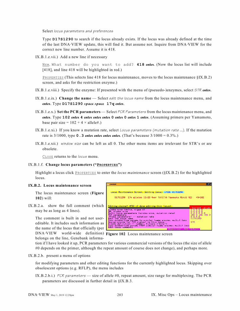
Figure 102 Locus maintenance screen
Select locus parameters and preferences
Type D17S1290 to search if the locus already exists. If the locus was already defined at the time
of the last DNA @VIEW update, this will find it. But assume not. Inquire from DNA@VIEW for the
correct new line number. Assume it is 418.
IX.B.1.e.vii.) Add a new line if necessary
NEW. What number do you want to add? 418 enter. (Now the locus list will include
[418], and line 418 will be highlighted in red.)
PROPERTIES (This selects line 418 for locus maintenance, moves to the locus maintenance §IX.B.2)
screen, and asks for the restriction enzyme.)
IX.B.1.e.viii.) Specify the enzyme: If presented with the menu of (pseuedo-)enzymes, select STR enter.
IX.B.1.e.ix.) Change the name — Select edit the locus name from the locus maintenance menu, and
enter. Type D17S1290 space space 17q enter.
IX.B.1.e.x.) Set the PCR parameters — Select PCR Parameters from the locus maintenance menu, and
enter. Type 102 enter 4 enter enter enter 0 enter 0 enter 1 enter. (Assuming primers per Yamamoto,
base pair size = 102 + 4 × allele#.)
IX.B.1.e.xi.) If you know a mutation rate, select Locus parameters (mutation rate ...). If the mutation
rate is 3/1000, type 0.3 enter enter enter enter. (That’s because 3/1000 = 0.3%.)
IX.B.1.e.xii.) window size can be left as all 0. The other menu items are irrelevant for STR’s or are
obsolete.
CLOSE returns to the locus menu.
IX.B.1.f. Change locus parameters (“PROPERTIES”)
Highlight a locus click PROPERTIES to enter the locus maintenance screen (§IX.B.2) for the highlighted
locus.
IX.B.2. Locus maintenance screen
The locus maintenance screen (Figure
102) will:
IX.B.2.a. show the full comment (which
may be as long as 4 lines).
The comment is built in and not user-
editable. It includes such information as
the name of the locus that officially (per
DNA @VIEW world-wide definition)
belongs on the line, Genebank informa-
tion if I have looked it up, PCR parameters for various commercial versions of the locus (the size of allele
#0 depends on the primer, although the repeat amount of course does not change), and perhaps more.
IX.B.2.b. present a menu of options
for modifying parameters and other editing functions for the currently highlighted locus. Skipping over
obsolescent options (e.g. RFLP), the menu includes
IX.B.2.b.i.) PCR parameters — size of allele #0, repeat amount, size range for multiplexing. The PCR
parameters are discussed in further detail in §IX.B.3.
DNA@VIEW May 1, 2019 12:29pm IX. Misc Ops – Locus maintenance203
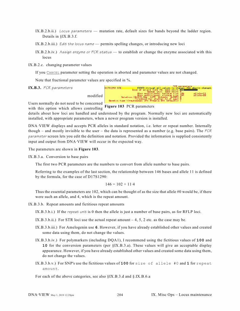
Figure 103 PCR parameters
IX.B.2.b.ii.) Locus parameters — mutation rate, default sizes for bands beyond the ladder region.
Details in §IX.B.3.f.
IX.B.2.b.iii.) Edit the locus name — permits spelling changes, or introducing new loci
IX.B.2.b.iv.) Assign enzyme or PCR status — to establish or change the enzyme associated with this
locus
IX.B.2.c. changing parameter values
If you CANCEL parameter setting the operation is aborted and parameter values are not changed.
Note that fractional parameter values are specified in %.
IX.B.3. PCR parameters
modified
Users normally do not need to be concerned
with this option which allows controlling
details about how loci are handled and understood by the program. Normally new loci are automatically
installed, with appropriate parameters, when a newer program version is installed.
DNA·VIEW displays and accepts PCR alleles in standard notation, i.e. letter or repeat number. Internally
though – and mostly invisible to the user – the data is represented as a number (e.g. base pairs). The PCR
parameter screen lets you edit the definition and notation. Provided the information is supplied consistently
input and output from DNAAVIEW will occur in the expected way.
The parameters are shown in Figure 103.
IX.B.3.a. Conversion to base pairs
The first two PCR parameters are the numbers to convert from allele number to base pairs.
Referring to the examples of the last section, the relationship between 146 bases and allele 11 is defined
by the formula, for the case of D17S1290:
146 = 102 + 11A4
Thus the essential parameters are 102, which can be thought of as the size that allele #0 would be, if there
were such an allele, and 4, which is the repeat amount.
IX.B.3.b. Repeat amounts and fictitious repeat amounts
IX.B.3.b.i.) If the repeat unit is 0 then the allele is just a number of base pairs, as for RFLP loci.
IX.B.3.b.ii.) For STR loci use the actual repeat amount – 4, 5, 2 etc. as the case may be.
IX.B.3.b.iii.) For Amelogenin use 6. However, if you have already established other values and created
some data using them, do not change the values.
IX.B.3.b.iv.) For polymarkers (including DQA1), I recommend using the fictitious values of 100 and
10 for the conversion parameters (per §IX.B.3.a). These values will give an acceptable display
appearance. However, if you have already established other values and created some data using them,
do not change the values.
IX.B.3.b.v.) For SNP's use the fictitious values of 100 for size of allele #0 and 1 for repeat
amount.
For each of the above categories, see also §IX.B.3.d and §.IX.B.6.a
DNA@VIEW May 1, 2019 12:29pm IX. Misc Ops – Locus maintenance204
IX.B.3.c. Multiplexing sizes
The third and fourth parameters, minimum and maximum size, are only necessary for purposes of
importing data such as GeneScan data where there may be several STR’s multiplexed in a single color.
The “multiplex” parameters can be specified when needed during the import process (§IX.B.3.c)
IX.B.3.d. Notation
The possible values for the Notation style parameter are defined as follows:
0 for STR, DQa or RFLP. Alleles are numbers, such as 12 or 1.2 or 5662.
If repeat unit > 0, then the normal display would be the conventional repeat number. For example
using the above parameters a 198 bp TH01 allele displays as 9.3. Format variations are possible
(Option Pcr notation style, §IX.F.28).
1 for polymarkers or equine loci. Alleles are letters A B C D ... Z. (However, the equine allele
O is sometimes shown on output as ò when the letter o would mean a null allele.)
2 for Amelogenin. Alleles are named X Y.
3 for SNP’s. Alleles are named G , A, C, T.
IX.B.3.e. SNP's
For the conversion parameters, see §IX.B.3.b.v. Select the value 3 for Notation, which corresponds
to alleles named G, A, C, and T.
Assign to SNPs the pseudo-enzyme SNP, which is [25] on the list.
IX.B.3.f. Genetic type
The genetic and other rules vary according to chromosome etc. Therefore the genetic category of loci is
specified, using the coding
1 autosomal
2 Y-chromosome
4 Sex marker, e.g. Amelogenin
8 X-chromosome
16 multi-locus probe
IX.B.4. Locus parameters (mutation, rare allele rates)
Select a probe and you can set certain parameters for that probe. The parameters are
IX.B.4.a. Paternal mutation rate :: rate of false exclusions (%)
ì is the percent of true fathers who would apparently be excluded by reason of mutation by this probe
system. The PI will then be computed as described in §XIII.B.6.
If the mutation rate is specified as 0, the default value (§V.C.3.g, V.C.3.h) applies.
IX.B.4.b. rare allele rate (only for Screening) (%)
This special feature is to cater to things like a historical designation of the TH01 “10" allele as “R”
(=rare), although in fact it is not “rare” in the usual DNA@VIEW sense of being nearly new. In that case,
use this parameter to specify, per locus, a minimum % frequency for such pseudo-rare alleles.
By default, Disaster Screening (§VII.D) treats off-ladder alleles (if imported as “rare” – see
§VII.B.2.b.ii) as new alleles and calculates their frequency according to the Count observed allele
(§V.C.4.a) and Minimum # (§V.C.4.b) Case options.
DNA@VIEW May 1, 2019 12:29pm IX. Misc Ops – Locus maintenance205
The frequency assumed by the Screening search will be the largest of the frequencies obtained by
considering each of the three parameters.
IX.B.5. Additional locus topics
IX.B.5.a. Locus name format
The first ten characters of the probe name are shown on all menus, and are generally the locus name. The
second ten characters can be used for chromosomal location name.
The only significance of the two parts is that on a PATER report (assuming that you have the PATER
software as well), the parts are shown separated by /.
IX.B.5.b. To change a locus, use the method described at §IX.B.2.b.iii.
DNA@VIEW May 1, 2019 12:29pm IX. Misc Ops – Locus maintenance206
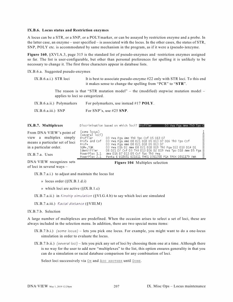
Figure 104 Multiplex selection
IX.B.6. Locus status and Restriction enzymes
A locus can be a STR, or a SNP, or a POLYmarker, or can be assayed by restriction enzyme and a probe. In
the latter case, an enzyme – user specified – is associated with the locus. In the other cases, the status of STR,
SNP, POLY etc. is accommodated by same mechanism in the program, as if it were a (pseudo-)enzyme.
Figure 160, §XVI.A.3, page 315 is the standard list of pseudo-enzymes and Arestriction enzymes assigned
so far. The list is user-configurable, but other than personal preferences for spelling it is unlikely to be
necessary to change it. The first three characters appear in database lists.
IX.B.6.a. Suggested pseudo-enzymes
IX.B.6.a.i.) STR loci It is best to associate pseudo-enzyme #22 only with STR loci. To this end
it makes sense to change the spelling from “PCR” to “STR”.
The reason is that “STR mutation model” – the (modified) stepwise mutation model –
applies to loci so categorized.
IX.B.6.a.ii.) Polymarkers For polymarkers, use instead #17 POLY.
IX.B.6.a.iii.) SNP For SNP’s, use #25 SNP.
IX.B.7. Multiplexes
From DNAAVIEW’s point of
view a multiplex simply
means a particular set of loci
in a particular order.
IX.B.7.a. Uses
DNAAVIEW recognizes sets
of loci in several ways –
IX.B.7.a.i.) to adjust and maintain the locus list
» locus order (§IX.B.1.d.i)
» which loci are active (§IX.B.1.c)
IX.B.7.a.ii.) in Kinship simulation (§VI.G.4.b) to say which loci are simulated
IX.B.7.a.iii.) Racial distance (§VIII.M)
IX.B.7.b. Selection
A large number of multiplexes are predefined. When the occasion arises to select a set of loci, these are
always included in the selection menu. In addition, there are two special menu items:
IX.B.7.b.i.) (some locus) – lets you pick one locus. For example, you might want to do a one-locus
simulation in order to evaluate the locus.
IX.B.7.b.ii.) (several loci) – lets you pick any set of loci by choosing them one at a time. Although there
is no way for the user to add new “multiplexes” to the list, this option ensures generality in that you
can do a simulation or racial database comparison for any combination of loci.
Select loci successively via OK and ADD ANOTHER until DONE.
DNA@VIEW May 1, 2019 12:29pm IX. Misc Ops – Locus maintenance207
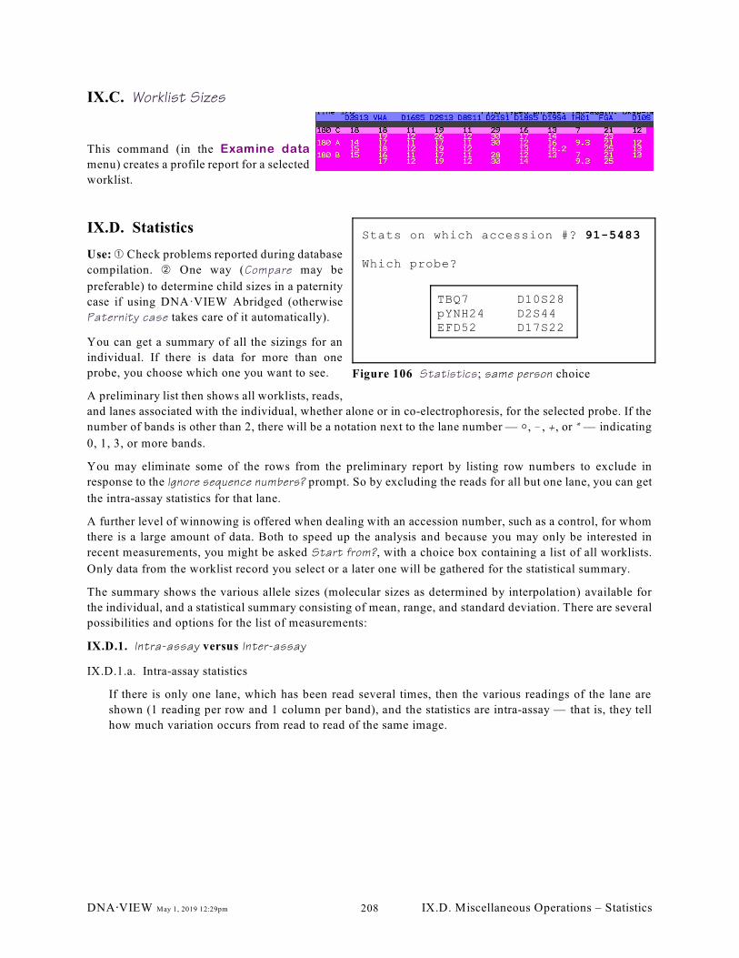
Stats on which accession #? 91-5483
Which probe?
TBQ7 D10S28pYNH24 D2S44EFD52 D17S22
Figure 106 Statistics; same person choice
IX.C. Worklist Sizes
This command (in the Examine data
menu) creates a profile report for a selected
worklist.
IX.D. Statistics
Use: â Check problems reported during database
compilation. ã One way (Compare may be
preferable) to determine child sizes in a paternity
case if using DNA·VIEW Abridged (otherwise
Paternity case takes care of it automatically).
You can get a summary of all the sizings for an
individual. If there is data for more than one
probe, you choose which one you want to see.
A preliminary list then shows all worklists, reads,
and lanes associated with the individual, whether alone or in co-electrophoresis, for the selected probe. If the
number of bands is other than 2, there will be a notation next to the lane number — N, !, +, or * — indicating
0, 1, 3, or more bands.
You may eliminate some of the rows from the preliminary report by listing row numbers to exclude in
response to the Ignore sequence numbers? prompt. So by excluding the reads for all but one lane, you can get
the intra-assay statistics for that lane.
A further level of winnowing is offered when dealing with an accession number, such as a control, for whom
there is a large amount of data. Both to speed up the analysis and because you may only be interested in
recent measurements, you might be asked Start from?, with a choice box containing a list of all worklists.
Only data from the worklist record you select or a later one will be gathered for the statistical summary.
The summary shows the various allele sizes (molecular sizes as determined by interpolation) available for
the individual, and a statistical summary consisting of mean, range, and standard deviation. There are several
possibilities and options for the list of measurements:
IX.D.1. Intra-assay versus Inter-assay
IX.D.1.a. Intra-assay statistics
If there is only one lane, which has been read several times, then the various readings of the lane are
shown (1 reading per row and 1 column per band), and the statistics are intra-assay — that is, they tell
how much variation occurs from read to read of the same image.
DNA@VIEW May 1, 2019 12:29pm IX.D. Miscellaneous Operations – Statistics208
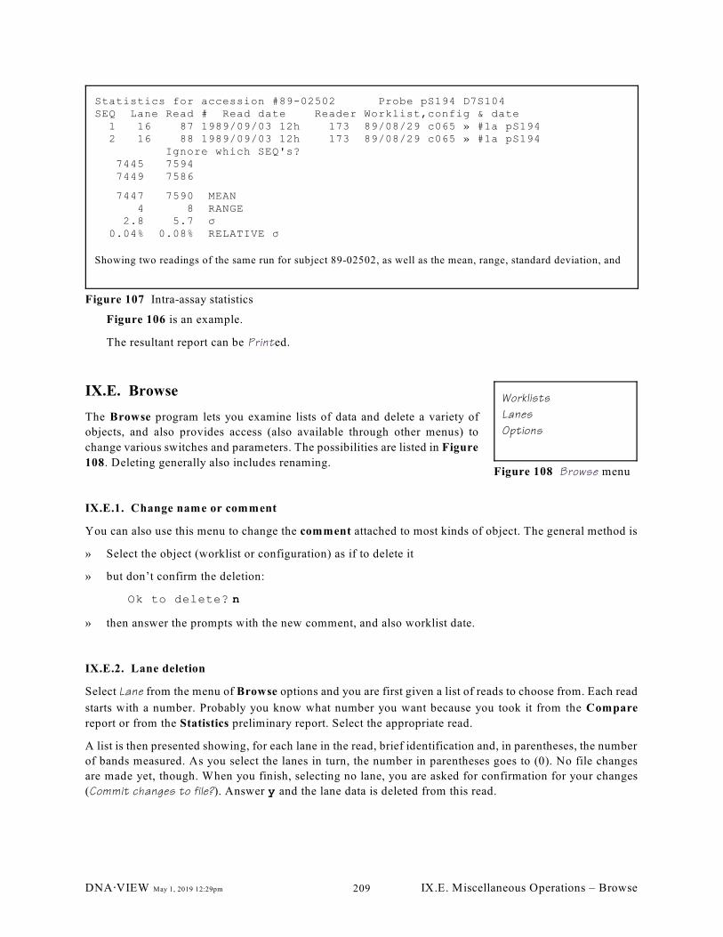
Statistics for accession #89-02502 Probe pS194 D7S104SEQ Lane Read # Read date Reader Worklist,config & date 1 16 87 1989/09/03 12h 173 89/08/29 c065 » #1a pS194 2 16 88 1989/09/03 12h 173 89/08/29 c065 » #1a pS194 Ignore which SEQ's? 7445 7594 7449 7586
7447 7590 MEAN 4 8 RANGE 2.8 5.7 ó 0.04% 0.08% RELATIVE ó
Showing two readings of the same run for subject 89-02502, as well as the mean, range, standard deviation, and
Figure 107 Intra-assay statistics
Worklists
Lanes
Options
Figure 108 Browse menu
Figure 106 is an example.
The resultant report can be Printed.
IX.E. Browse
The Browse program lets you examine lists of data and delete a variety of
objects, and also provides access (also available through other menus) to
change various switches and parameters. The possibilities are listed in Figure
108. Deleting generally also includes renaming.
IX.E.1. Change name or comment
You can also use this menu to change the comment attached to most kinds of object. The general method is
» Select the object (worklist or configuration) as if to delete it
» but don’t confirm the deletion:
Ok to delete? n
» then answer the prompts with the new comment, and also worklist date.
IX.E.2. Lane deletion
Select Lane from the menu of Browse options and you are first given a list of reads to choose from. Each read
starts with a number. Probably you know what number you want because you took it from the Compare
report or from the Statistics preliminary report. Select the appropriate read.
A list is then presented showing, for each lane in the read, brief identification and, in parentheses, the number
of bands measured. As you select the lanes in turn, the number in parentheses goes to (0). No file changes
are made yet, though. When you finish, selecting no lane, you are asked for confirmation for your changes
(Commit changes to file?). Answer y and the lane data is deleted from this read.
DNA@VIEW May 1, 2019 12:29pm IX.E. Miscellaneous Operations – Browse209
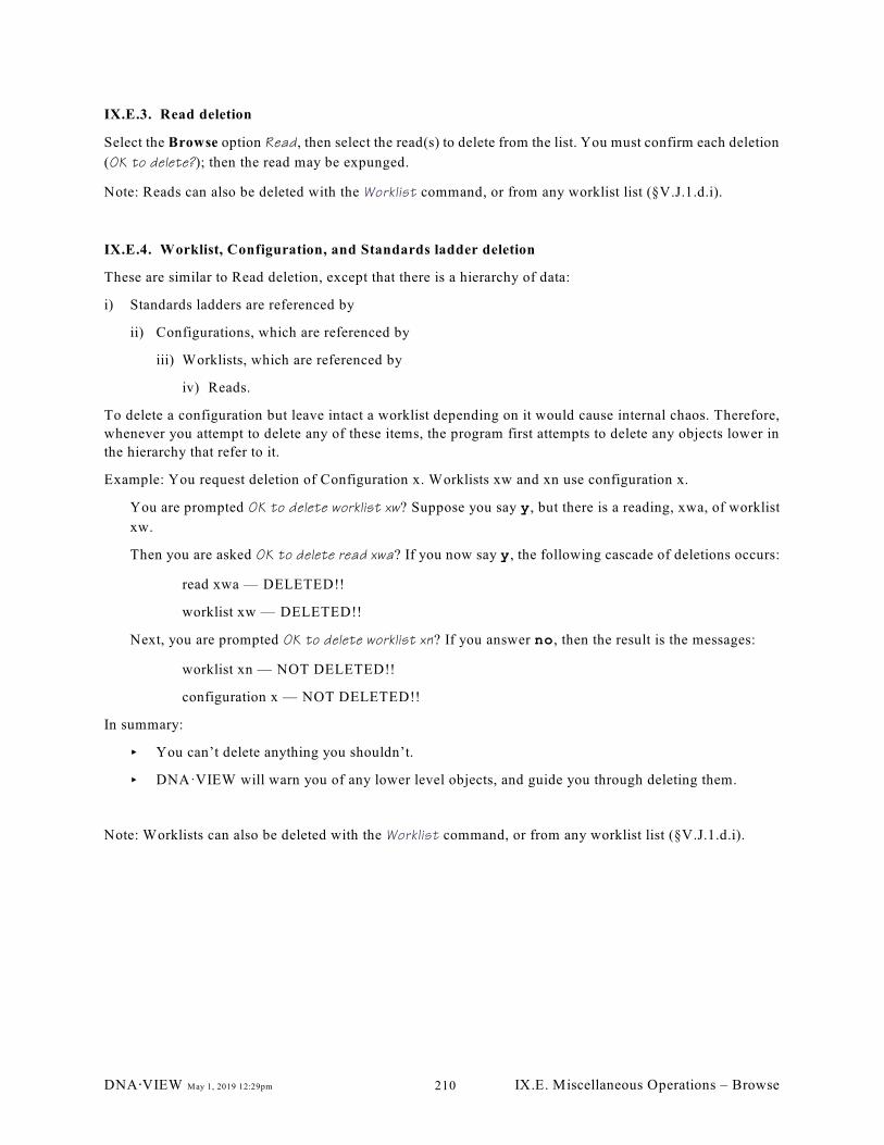
IX.E.3. Read deletion
Select the Browse option Read, then select the read(s) to delete from the list. You must confirm each deletion
(OK to delete?); then the read may be expunged.
Note: Reads can also be deleted with the Worklist command, or from any worklist list (§V.J.1.d.i).
IX.E.4. Worklist, Configuration, and Standards ladder deletion
These are similar to Read deletion, except that there is a hierarchy of data:
i) Standards ladders are referenced by
ii) Configurations, which are referenced by
iii) Worklists, which are referenced by
iv) Reads.
To delete a configuration but leave intact a worklist depending on it would cause internal chaos. Therefore,
whenever you attempt to delete any of these items, the program first attempts to delete any objects lower in
the hierarchy that refer to it.
Example: You request deletion of Configuration x. Worklists xw and xn use configuration x.
You are prompted OK to delete worklist xw? Suppose you say y, but there is a reading, xwa, of worklist
xw.
Then you are asked OK to delete read xwa? If you now say y, the following cascade of deletions occurs:
read xwa — DELETED!!
worklist xw — DELETED!!
Next, you are prompted OK to delete worklist xn? If you answer no, then the result is the messages:
worklist xn — NOT DELETED!!
configuration x — NOT DELETED!!
In summary:
< You can’t delete anything you shouldn’t.
< DNA·VIEW will warn you of any lower level objects, and guide you through deleting them.
Note: Worklists can also be deleted with the Worklist command, or from any worklist list (§V.J.1.d.i).
DNA@VIEW May 1, 2019 12:29pm IX.E. Miscellaneous Operations – Browse210
IX.F. Options
This command is a miscellany of functionalities that you can specify to control program operation.
IX.F.1. Box drawing characters
Three alternative drawing choices are available for box borders (e.g. when DNA@VIEW puts a box around a
result in an immigration/kinship report:
IX.F.1.a. The box drawing characters +),.)-*5 are attractive if available but some national display or
printing modes don't have them and the result is very unattractive. In that case choose one of these
alternative:
IX.F.1.b. Symbols + ! | > as an approximate way to draw box borders, or
IX.F.1.c. (none) – leave the borders off. This is an improved alternative to §IX.F.8.c.
IX.F.2. Case # format: 09/00123
new
This option lets you set three parameters governing case number appearance (format).
DNA@VIEW (and PATER) case numbers may be any integer from 1 up to about 2100000000 (that’s 10 digits,
and the exact limitation is 4-byte computer integers, i.e. case#<2 ). This allows for example a 4-digit year and31
6 more digits of sequence number within the year.
For convenience of input and viewing appearance the case number can be broken into two parts with any
character you wish separating them.
IX.F.2.a. The case number format parameters are
Y: leading (“year”) digits? (typically choices are 2 or 4)
Y controls two things: (a) leading 0 padding on display of a case number, (b) the meaning of the
special case number “year” input buttons per §V.B.28.a.iii. Note that if you want to type in the year
you can use as many digits as you wish, not even necessarily relating to a year. For example
12345/12345 can be legal case number.
N: trailing (sequence) digit positions? 5
N controls (a) 0-padding after the separator on display of a case number (i.e. 09/00123 rather than
09/123), (b) minimum number of digit positions for the sequence part when you use a special input
key L T or N to prefix a year code without typing the year.
S: Separator character(s). (First one is for output; all for input.) /.-
The first separator is the main one, which the program will use for display of case numbers. The others
are just extra options that you can use for typing in case numbers.
» Display appearance is determined mostly by the parameter N and the first S. The full integer case
number is written. If there are more than N digits, then the first separator is placed before the final
N digits. If the result is fewer than Y digits (but at least 1 digit) before the separator, then
additional 0 's are padded to the left.
There may be more than Y digits before the separator.
» Input. When entering a case number there are several possibilities:
• Type in as many digits as you wish, e.g. 200901234
DNA@VIEW May 1, 2019 12:29pm IX.F. Miscellaneous operations – Options211
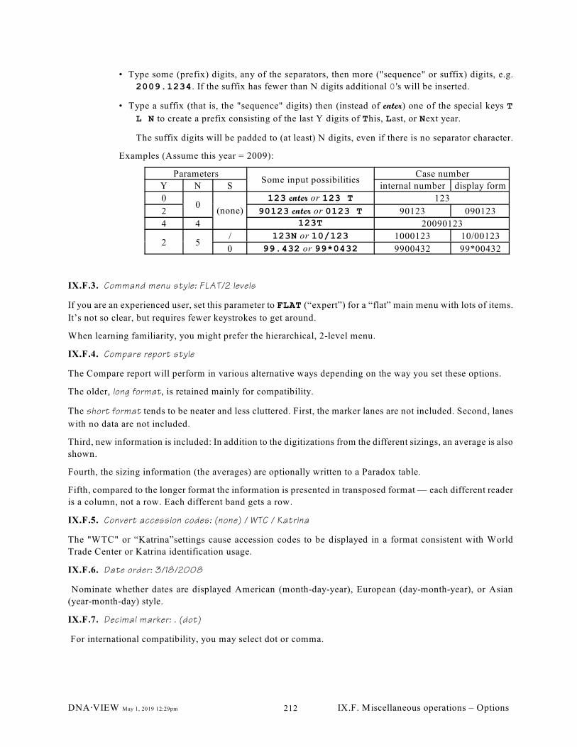
• Type some (prefix) digits, any of the separators, then more ("sequence" or suffix) digits, e.g.
2009.1234. If the suffix has fewer than N digits additional 0 's will be inserted.
• Type a suffix (that is, the "sequence" digits) then (instead of enter) one of the special keys T
L N to create a prefix consisting of the last Y digits of This, Last, or Next year.
The suffix digits will be padded to (at least) N digits, even if there is no separator character.
Examples (Assume this year = 2009):
ParametersSome input possibilities
Case number
Y N S internal number display form
00
(none)
123 enter or 123 T 123
2 90123 enter or 0123 T 90123 090123
4 4 123T 20090123
2 5/ 123N or 10/123 1000123 10/00123
0 99.432 or 99*0432 9900432 99*00432
IX.F.3. Command menu style: FLAT/2 levels
If you are an experienced user, set this parameter to FLAT (“expert”) for a “flat” main menu with lots of items.
It’s not so clear, but requires fewer keystrokes to get around.
When learning familiarity, you might prefer the hierarchical, 2-level menu.
IX.F.4. Compare report style
The Compare report will perform in various alternative ways depending on the way you set these options.
The older, long format, is retained mainly for compatibility.
The short format tends to be neater and less cluttered. First, the marker lanes are not included. Second, lanes
with no data are not included.
Third, new information is included: In addition to the digitizations from the different sizings, an average is also
shown.
Fourth, the sizing information (the averages) are optionally written to a Paradox table.
Fifth, compared to the longer format the information is presented in transposed format — each different reader
is a column, not a row. Each different band gets a row.
IX.F.5. Convert accession codes: (none) / WTC / Katrina
The "WTC" or “Katrina”settings cause accession codes to be displayed in a format consistent with World
Trade Center or Katrina identification usage.
IX.F.6. Date order: 3/18/2008
Nominate whether dates are displayed American (month-day-year), European (day-month-year), or Asian
(year-month-day) style.
IX.F.7. Decimal marker: . (dot)
For international compatibility, you may select dot or comma.
DNA@VIEW May 1, 2019 12:29pm IX.F. Miscellaneous operations – Options212
IX.F.8. DNA@VIEW character translation
IX.F.8.a. Symbol sets
Accented characters sometimes fail to print correctly because of the printer using a “symbol set” different
from the symbol set used on the display monitor. The display monitor symbol set is called “PC-8”, and
has for example the symbols ü and é as ASCII codes 129 and 130. If the printer is also operating with the
PC-8 symbol set, then no translation is necessary.
However, there are also other symbol sets — especially used with languages that have many accented
characters — and they differ from PC-8 with respect to the symbols that correspond to the ASCII codes,
especially the upper half of the ASCII table from 128!255. For example, the HP Roman 8 symbol set
includes extra accented characters, omits the line drawing characters, and the symbols ü and é are ASCII
codes 207 and 197.
IX.F.8.b. Translation mechanism
Therefore, in order to allow these and other characters to print correctly or nearly so on a printer that is
not using the PC-8 symbol set, a translation mechanism is provided. This option provides a mechanism
whereby the numeric ASCII code for each screen character can be translated into a different numeric code
when printing.
The mechanism provides a menu of the higher ASCII codes, from 128!255. Select a code from the menu,
then respond to the prompt to give the new ASCII value. When done with selections, make the empty
selection and only then will the new translation table be filed.
While you can assign any translation codes you like, the program has some intelligence and knows what
the likely translation is based on your choice of language (see §IX.F.18). If a character is currently listed
in the table as untranslated, the likely translation will be suggested as a default.
IX.F.8.c. Box-drawing characters
Depending on the printer settings, those characters that make elegant borders on the screen may look like
garbage on the printed page. You can get rid of them by specifying a translation to 0. This doesn’t actually
introduce 0 characters (nulls) into the output; it simply suppresses the character. Deprecated – easier to
use §IX.F.1.
IX.F.9. DNA@VIEW Printer
Change the kind of printer used for reports (not graphics) — the printer that DNA@VIEW will assume it’s
talking to when you Print. The main options are
» Laser to print directly to a Laserjet, Deskjet, or compatible printer;
» PrintFil to print in cooperation with the PrintFil software. See §XV.D.3.a for more details.
To specify the kind of printer for purposes of graphics (e.g. printing images from Plot, §VIII.E), you have to
edit the CGI.CFG file (XV.D.6). But see METAFIL, §VIII.E.1.b.v.
IX.F.10. DNA@VIEW Printer port
Possibilities:
» (Display on screen) defers the choice until each time you print (see §V.K.1),
» print via PrintFil will, if the PrintFil (see §XV.D.3.a) software is installed, send the image to PrintFil
for processing and printing,
DNA@VIEW May 1, 2019 12:29pm IX.F. Miscellaneous operations – Options213
» LPT1, LPT2 print via (probably virtual versions of) these traditional ports. To print to USB, choose
either of these and see §XV.D.2.a.v.
IX.F.11. DNA@VIEW report title line
With this option you can change the report title of the printed reports. It is possible to create a fancy title with
varying fonts or sizes by inserting printer control codes – e.g. PCL for a LaserJet or Deskjet printer. As part
of these codes you will need to insert the non-typeable character Esc. For this purpose you can type { as a
surrogate, which will be translated to Esc.
IX.F.12. DNAAVIEW report includes: [Version, Workstation]
For better tracking and documentation of the reports that get printed by DNAAVIEW, you may elect that the
DNAAVIEW version number and/or the network name (see Network, §XV.D) of the workstation from which
the report is printed be included on the first page of each report.
IX.F.13. DNA@VIEW report epilogue
The epilogue is a technical facility. If for example DNA@VIEW is sharing the printer with other users and needs
to send a special printer sequence after each use of the printer, this is the place to put that sequence.
IX.F.14. Default date?
If you choose y then you can enter new accession numbers faster because Enter will accept today’s date as a
default. On the other hand, if you are serious about the accession date — perhaps it is part of your documenta-
tion — then choose n here to minimize errors on input.
IX.F.15. Graphics detail scaling
If your printer is a deskjet some of the graphic output looks better if you set this parameter to 0.5. Otherwise,
it should be 1.
IX.F.16. Interpolation parameters
Using an allelic ladder, molecular sizes are usually determined according to three flanking markers. Otherwise,
eight markers are used for a globally fitting curve.
You can experiment with other choices than 3 and 8 using this option.
IX.F.17. Keyboard
The Keyboard choice lets the user choose among various national keyboards. There are a variety of special
keyboard drivers, not guaranteed to work ideally. To switch from one choice to another it may be necessary
to exit from the program, especially when to simply remove a driver via the choice (none).
IX.F.18. Language
Some of the menus, explanations, and report paragraphs have multi!lingual options. Choose which language
you prefer.
IX.F.19. Locus name style like: D16S539 STR
Four formatting choices for locus name display are offered:
(a) The bare locus name, such as D16S539, or:
(b) Include the chromosomal information, and/or
(c) Include the category such as STR.
DNA@VIEW May 1, 2019 12:29pm IX.F. Miscellaneous operations – Options214
IX.F.20. Locus parameters
This option is equivalent to Maintenance option of the same name described in §IX.B.
IX.F.21. Message display time
Sometimes DNA@VIEW pops up a message for a limited time (maybe 1 or 3 seconds by default depending on
the message). Set this value to 10 seconds to give yourself lots of time to read (anyway space when the
message appears will hurry it along), or 0 for the default times.
IX.F.22. Minimum frequency parameters
Same as Options from "Case" (§V.C)
IX.F.23. Name tag style: NAME/DATE
Toggle whether the name tag block – the list of people in a case – displays an accession date, or the name of
the person.
IX.F.24. Numlock on/off
Reverse the default state of the “numlock” key.
IX.F.25. Off-ladder allele policy: DISCARD/RARE(revised – 2014)
When importing DNA profiles (§X.A – using e.g. Genotyper import), what happens when an illegal notation
(such as "?" or "OL" or "OL13.2") is encountered. Three choices, which roughly corresponding to ignoring
2, 0, and 1 allele at the locus:
» Discard genotype if it includes "ol", "?" or other garbage means that the allele and it's companion
(i.e the genotype for the locus for that person) are ignored and not imported.
» Treat "ol", "?" etc as a rare allele (but "OL13" as 13) means that the allele will be treated as a rare
allele not found in any database. Rare alleles will match one another, however.
» Ignore "OL", "?" etc (as if blank); treat "OL13" as 13. The illegal notation is ignored and the other
allele (if any) is imported. Most DNA@VIEW calculations treat the single allele as a homozygous
type, though sometimes a null allele is allowed for also.
IX.F.26. Options from "Case"
This is an alternative way to access the same options that are accessible as Options from the Pater-
nity/Automatic mixture or Automatic Kinship sub!menu (discussed in §V.C).
IX.F.27. PCR allele binning? NO/YES
This obsolescent option controls whether “allele resolution filters” are active. If it is set to yes, then all sizes
are resolved, if possible, before being used for casework, creating databases, etc. If it is set to no, then raw
sizes as stored are used.
IX.F.28. PCR notation style
Using this option from the Options submenu, you can choose how PCR sizes will be formatted for output.
PCR sizes are shown as base pairs (optionally), and (also) as an estimated allele number and discrepancy.
IX.F.28.a. Round/Truncate
IX.F.28.a.i.) Truncate size to estimate allele number, offset alwayspositive: "17.15"
DNA@VIEW May 1, 2019 12:29pm IX.F. Miscellaneous operations – Options215
An allele is shown as a positive (or zero) discrepancy from the next lower integer allele. For example,
the common TH01 variant allele will print as 9·3 even though it is closer to 10 than to 9. This option
is consistent with standard usage in the literature.
IX.F.28.a.ii.) Round the sizes to estimate the allele number, offset may be
negative: "18.-1" (obsolete – do not use)
IX.F.28.b. Short/Long notation
Choose the “short” format (e.g. 20.9). “Long” is obsolete.
IX.F.28.c. Omit/Show odd base pairs
If the size is an exact number of repeats, you can choose to display (i.e. 18.0) or to omit (just 18)
displaying the 0 odd base pairs. The second way is probably more readable. The first alternative is
included mainly in case you will be passing the sizes along to another computer program (i.e. using the
Compare report).
IX.F.28.d. decimals
In case the allele is represented, for whatever reason, as a non-integer number of base pairs, you can show
0, 1, or 2 decimal digits.
IX.F.28.e. separator – (period is universally standard)
To display a fractional repeat amount, several choices are possible: 9A3 or 9.3 or 9,3.
IX.F.29. page format
This controls how various reports use the paper. If the printer is a laserJet, even the type size can vary in order
to fit the report better on the paper. You specify
IX.F.29.a. Normal type, chars/inch, (usu 12) for the standard type size.
IX.F.29.b. Maximum chars/inch, (rec 20) permits a smaller type to be used to avoid line wrapping, such as
for the “RAW FRAGMENTS” section of the paternity report.
IX.F.29.c. Left margin columns (rec >3) is the left margin in “normal” columns.
IX.F.29.d. Column positions printable (US<87, A4<84) again are in units of the “normal” type. The numbers
in parentheses correspond to 0 right margin, so at least 3 fewer is recommended.
IX.F.29.e. Lines/page (US<69, A4<74). Again, the given figures will result in no bottom margin, so subtract
a few lines. Alternatively, you may specify an essentially infinite page such as 9999 lines to defeat
DNA@VIEW’s pagination attempts and page headings. The printer will then start a new page when
necessary.
IX.F.29.f. Use Natural page breaks, or Full pages to save paper? Natural breaks means avoid breaking a
logical section across pages. Full page means conserve paper, but harder to read.
IX.F.30. Paradox directory
Best practice and normal installation is to specify pdox\ as the location where that Paradox tables are kept.
This relative notation denotes a subfolder of the installation folder for DNA@VIEW. Using relative notation
ensures that no change will be needed if DNAAVIEW is migrated to a new location.
DNA@VIEW May 1, 2019 12:29pm IX.F. Miscellaneous operations – Options216
IX.F.31. PATER character translation
This option controls the character codes that are used for PATER reports, and doesn’t affect DNA @VIEW at
all. Operation is as described in §IX.F.8.
IX.F.32. PATER signature line
IX.F.33. PATER Logo
These options are only useful if you are using the PATER program to generate reports. They allow you to
specify some of the boilerplate on the PATER report.
IX.F.34. Plot line thickness
This controls the thickness, in pixels, of lines in data base plots (§VIII.E). A value of 1 gives a narrow line,
100 or 200 gives a very bold one, 2000 looks rather amusing like advertising copy.
IX.F.35. RFLP: disabled
Some menu options that are useful only for RFLP work are hidden; switch to enabled to see them.
IX.F.36. Window style
This option defines the way that DNA@VIEW interprets the window size parameter delta (ä) for probability
computations.
For discrete allele systems either ä=0 or at most ä is very small. In either case the alternatives for windows size
interpretation probably have exactly the same result.
Recommended window style is the best choice.
DNA@VIEW May 1, 2019 12:29pm IX.F. Miscellaneous operations – Options217
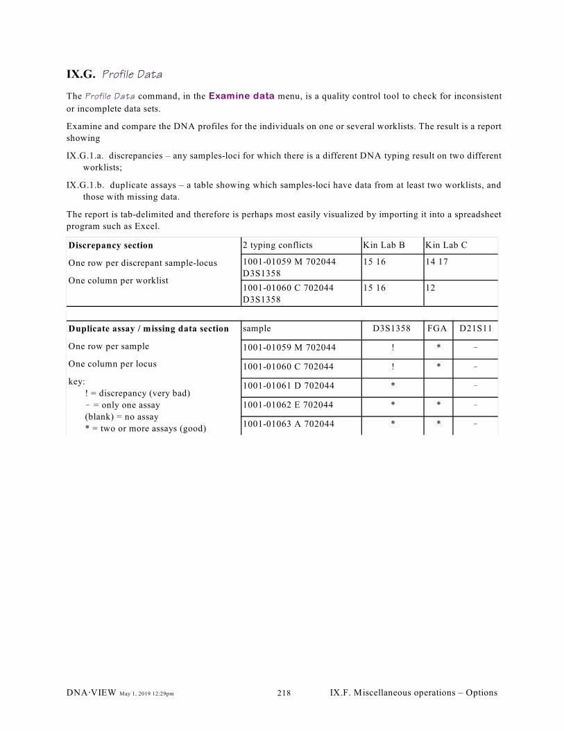
IX.G. Profile Data
The Profile Data command, in the Examine data menu, is a quality control tool to check for inconsistent
or incomplete data sets.
Examine and compare the DNA profiles for the individuals on one or several worklists. The result is a report
showing
IX.G.1.a. discrepancies – any samples-loci for which there is a different DNA typing result on two different
worklists;
IX.G.1.b. duplicate assays – a table showing which samples-loci have data from at least two worklists, and
those with missing data.
The report is tab-delimited and therefore is perhaps most easily visualized by importing it into a spreadsheet
program such as Excel.
Discrepancy section
One row per discrepant sample-locus
One column per worklist
2 typing conflicts Kin Lab B Kin Lab C
1001-01059 M 702044
D3S1358
15 16 14 17
1001-01060 C 702044
D3S1358
15 16 12
Duplicate assay / missing data section
One row per sample
One column per locus
key:
! = discrepancy (very bad)
! = only one assay
(blank) = no assay
* = two or more assays (good)
sample D3S1358 FGA D21S11
1001-01059 M 702044 ! * !
1001-01060 C 702044 ! * !
1001-01061 D 702044 * !
1001-01062 E 702044 * * !
1001-01063 A 702044 * * !
DNA@VIEW May 1, 2019 12:29pm IX.F. Miscellaneous operations – Options218
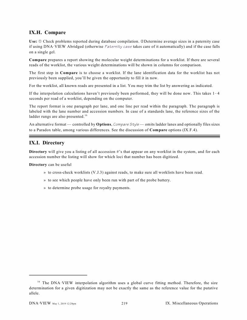
IX.H. Compare
Use: â Check problems reported during database compilation. ãDetermine average sizes in a paternity case
if using DNA·VIEW Abridged (otherwise Paternity case takes care of it automatically) and if the case falls
on a single gel.
Compare prepares a report showing the molecular weight determinations for a worklist. If there are several
reads of the worklist, the various weight determinations will be shown in columns for comparison.
The first step in Compare is to choose a worklist. If the lane identification data for the worklist has not
previously been supplied, you’ll be given the opportunity to fill it in now.
For the worklist, all known reads are presented in a list. You may trim the list by answering as indicated.
If the interpolation calculations haven’t previously been performed, they will be done now. This takes 1!4
seconds per read of a worklist, depending on the computer.
The report format is one paragraph per lane, and one line per read within the paragraph. The paragraph is
labeled with the lane number and accession numbers. In case of a standards lane, the reference sizes of the
ladder rungs are also presented.16
An alternative format — controlled by Options, Compare Style — omits ladder lanes and optionally files sizes
to a Paradox table, among various differences. See the discussion of Compare options (IX.F.4).
IX.I. Directory
Directory will give you a listing of all accession #’s that appear on any worklist in the system, and for each
accession number the listing will show for which loci that number has been digitized.
Directory can be useful
» to cross-check worklists (V.J.3) against reads, to make sure all worklists have been read.
» to see which people have only been run with part of the probe battery.
» to determine probe usage for royalty payments.
The DNA·VIEW interpolation algorithm uses a global curve fitting method. Therefore, the size16
determination for a given digitization may not be exactly the same as the reference value for the putative
allele.
DNA@VIEW May 1, 2019 12:29pm IX. Miscellaneous Operations219
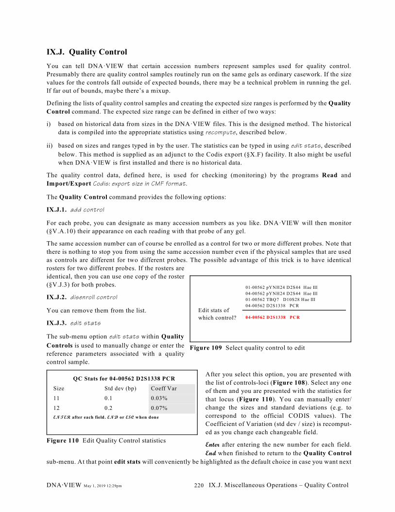
01-00562 pYNH24 D2S44 Hae III
04-00562 pYNH24 D2S44 Hae III
01-00562 TBQ7 D10S28 Hae III
04-00562 D2S1338 PCREdit stats of
which control? 04-00562 D2S1338 PCR
Figure 109 Select quality control to edit
QC Stats for 04-00562 D2S1338 PCR
Size Std dev (bp) Coeff Var
11 0.1 0.03%
12 0.2 0.07%
ENTER after each field. END or ESC when done
Figure 110 Edit Quality Control statistics
IX.J. Quality Control
You can tell DNA·VIEW that certain accession numbers represent samples used for quality control.
Presumably there are quality control samples routinely run on the same gels as ordinary casework. If the size
values for the controls fall outside of expected bounds, there may be a technical problem in running the gel.
If far out of bounds, maybe there’s a mixup.
Defining the lists of quality control samples and creating the expected size ranges is performed by the Quality
Control command. The expected size range can be defined in either of two ways:
i) based on historical data from sizes in the DNA·VIEW files. This is the designed method. The historical
data is compiled into the appropriate statistics using recompute, described below.
ii) based on sizes and ranges typed in by the user. The statistics can be typed in using edit stats, described
below. This method is supplied as an adjunct to the Codis export (§X.F) facility. It also might be useful
when DNA·VIEW is first installed and there is no historical data.
The quality control data, defined here, is used for checking (monitoring) by the programs Read and
Import/Export Codis: export size in CMF format.
The Quality Control command provides the following options:
IX.J.1. add control
For each probe, you can designate as many accession numbers as you like. DNA·VIEW will then monitor
(§V.A.10) their appearance on each reading with that probe of any gel.
The same accession number can of course be enrolled as a control for two or more different probes. Note that
there is nothing to stop you from using the same accession number even if the physical samples that are used
as controls are different for two different probes. The possible advantage of this trick is to have identical
rosters for two different probes. If the rosters are
identical, then you can use one copy of the roster
(§V.J.3) for both probes.
IX.J.2. disenroll control
You can remove them from the list.
IX.J.3. edit stats
The sub-menu option edit stats within Quality
Controls is used to manually change or enter the
reference parameters associated with a quality
control sample.
After you select this option, you are presented with
the list of controls-loci (Figure 108). Select any one
of them and you are presented with the statistics for
that locus (Figure 110). You can manually enter/
change the sizes and standard deviations (e.g. to
correspond to the official CODIS values). The
Coefficient of Variation (std dev / size) is recomput-
ed as you change each changeable field.
Enter after entering the new number for each field.
End when finished to return to the Quality Control
sub-menu. At that point edit stats will conveniently be highlighted as the default choice in case you want next
DNA@VIEW May 1, 2019 12:29pm IX.J. Miscellaneous Operations – Quality Control220
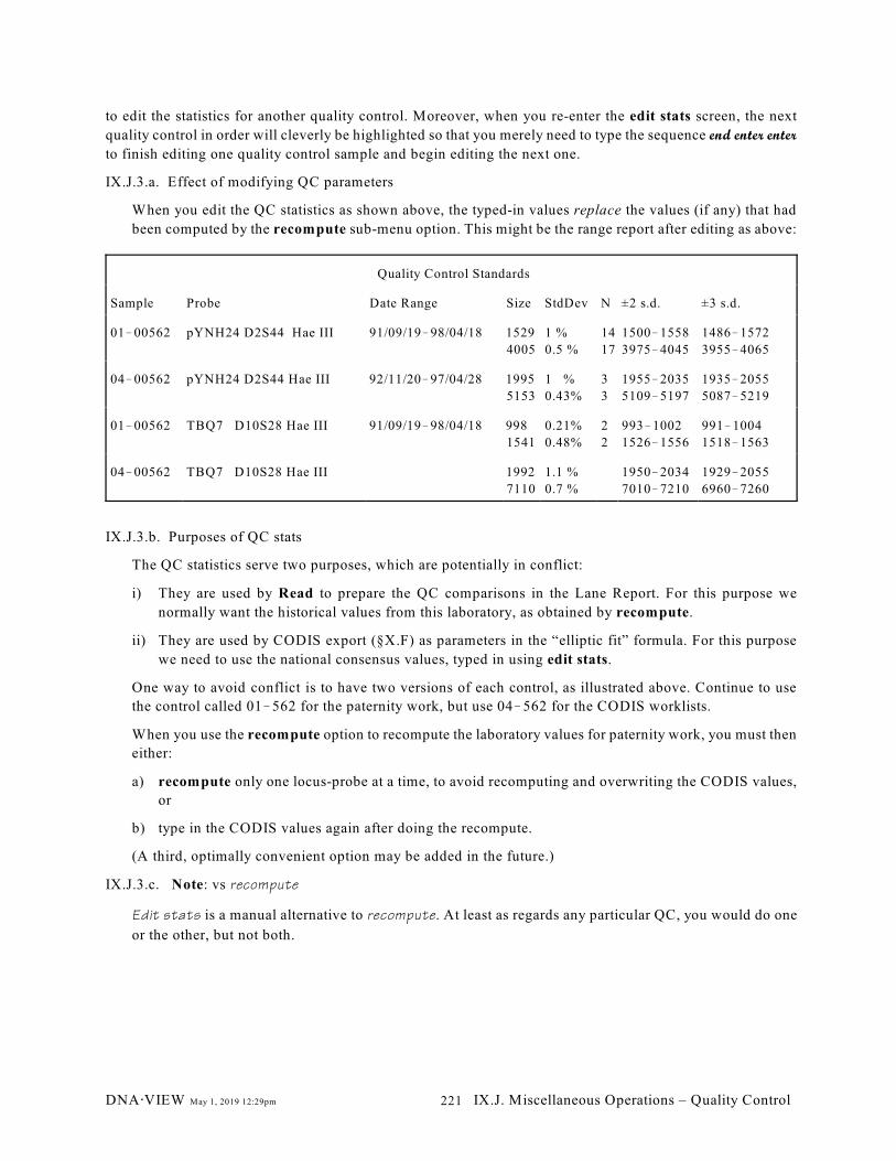
Quality Control Standards
Sample Probe Date Range Size StdDev N ±2 s.d. ±3 s.d.
01!00562 pYNH24 D2S44 Hae III 91/09/19!98/04/18 1529
4005
1 %
0.5 %
14
17
1500!1558
3975!4045
1486!1572
3955!4065
04!00562 pYNH24 D2S44 Hae III 92/11/20!97/04/28 1995
5153
1 %
0.43%
3
3
1955!2035
5109!5197
1935!2055
5087!5219
01!00562 TBQ7 D10S28 Hae III 91/09/19!98/04/18 998
1541
0.21%
0.48%
2
2
993!1002
1526!1556
991!1004
1518!1563
04!00562 TBQ7 D10S28 Hae III 1992
7110
1.1 %
0.7 %
1950!2034
7010!7210
1929!2055
6960!7260
to edit the statistics for another quality control. Moreover, when you re-enter the edit stats screen, the next
quality control in order will cleverly be highlighted so that you merely need to type the sequence end enter enter
to finish editing one quality control sample and begin editing the next one.
IX.J.3.a. Effect of modifying QC parameters
When you edit the QC statistics as shown above, the typed-in values replace the values (if any) that had
been computed by the recompute sub-menu option. This might be the range report after editing as above:
IX.J.3.b. Purposes of QC stats
The QC statistics serve two purposes, which are potentially in conflict:
i) They are used by Read to prepare the QC comparisons in the Lane Report. For this purpose we
normally want the historical values from this laboratory, as obtained by recompute.
ii) They are used by CODIS export (§X.F) as parameters in the “elliptic fit” formula. For this purpose
we need to use the national consensus values, typed in using edit stats.
One way to avoid conflict is to have two versions of each control, as illustrated above. Continue to use
the control called 01!562 for the paternity work, but use 04!562 for the CODIS worklists.
When you use the recompute option to recompute the laboratory values for paternity work, you must then
either:
a) recompute only one locus-probe at a time, to avoid recomputing and overwriting the CODIS values,
or
b) type in the CODIS values again after doing the recompute.
(A third, optimally convenient option may be added in the future.)
IX.J.3.c. Note: vs recompute
Edit stats is a manual alternative to recompute. At least as regards any particular QC, you would do one
or the other, but not both.
DNA@VIEW May 1, 2019 12:29pm IX.J. Miscellaneous Operations – Quality Control221
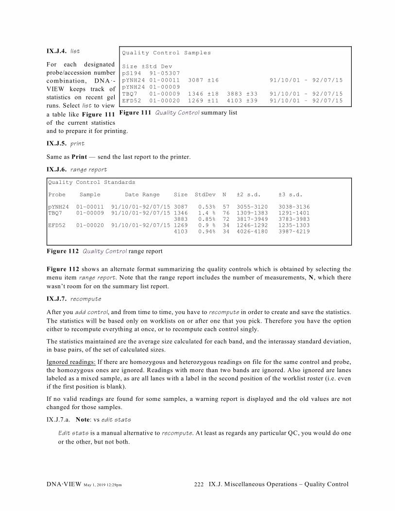
Quality Control Samples
Size ±Std DevpS194 91!05307 pYNH24 01!00011 3087 ±16 91/10/01 ! 92/07/15pYNH24 01!00009 TBQ7 01!00009 1346 ±18 3883 ±33 91/10/01 ! 92/07/15EFD52 01!00020 1269 ±11 4103 ±39 91/10/01 ! 92/07/15
Figure 111 Quality Control summary list
Quality Control Standards
Probe Sample Date Range Size StdDev N ±2 s.d. ±3 s.d.
pYNH24 01!00011 91/10/01!92/07/15 3087 0.53% 57 3055!3120 3038!3136TBQ7 01!00009 91/10/01!92/07/15 1346 1.4 % 76 1309!1383 1291!1401 3883 0.85% 72 3817!3949 3783!3983EFD52 01!00020 91/10/01!92/07/15 1269 0.9 % 34 1246!1292 1235!1303 4103 0.94% 34 4026!4180 3987!4219
Figure 112 Quality Control range report
IX.J.4. list
For each designated
probe/accession number
combination, DNA·-
VIEW keeps track of
statistics on recent gel
runs. Select list to view
a table like Figure 111
of the current statistics
and to prepare it for printing.
IX.J.5. print
Same as Print — send the last report to the printer.
IX.J.6. range report
Figure 112 shows an alternate format summarizing the quality controls which is obtained by selecting the
menu item range report. Note that the range report includes the number of measurements, N, which there
wasn’t room for on the summary list report.
IX.J.7. recompute
After you add control, and from time to time, you have to recompute in order to create and save the statistics.
The statistics will be based only on worklists on or after one that you pick. Therefore you have the option
either to recompute everything at once, or to recompute each control singly.
The statistics maintained are the average size calculated for each band, and the interassay standard deviation,
in base pairs, of the set of calculated sizes.
Ignored readings: If there are homozygous and heterozygous readings on file for the same control and probe,
the homozygous ones are ignored. Readings with more than two bands are ignored. Also ignored are lanes
labeled as a mixed sample, as are all lanes with a label in the second position of the worklist roster (i.e. even
if the first position is blank).
If no valid readings are found for some samples, a warning report is displayed and the old values are not
changed for those samples.
IX.J.7.a. Note: vs edit stats
Edit stats is a manual alternative to recompute. At least as regards any particular QC, you would do one
or the other, but not both.
DNA@VIEW May 1, 2019 12:29pm IX.J. Miscellaneous Operations – Quality Control222
IX.J.8. show details
As a side effect, recompute saves the individual band sizes lane by lane for each control. It is very useful to
look at this list if the statistics happen to be suspicious. If there are one or two aberrant numbers, you can
quickly find them and note the worklist and lane from which they come. This information, coupled with
Compare or Flash and Browse (delete lanes) makes it easy to clean up the data.
DNA@VIEW May 1, 2019 12:29pm IX.J. Miscellaneous Operations – Quality Control223

DNA@VIEW May 1, 2019 12:29pm IX.J. Miscellaneous Operations – Quality Control224
X. IMPORT/EXPORT
This chapter describes the various options of the Import/Export command. Since there are about twenty
options it is convenient to group them into categories.
§X.A DNA profile data import (case, worklist, mixture); various formats.. . . . . . . . . . . . . . . . . . . . . . 226
§X.A.1 Genotyper import. . . . . . . . . . . . . . . . . . . . . . . . . . . . . . . . . . . . . . . . . . . . . . . . . . . 226
§X.A.5 GeneMapper import. . . . . . . . . . . . . . . . . . . . . . . . . . . . . . . . . . . . . . . . . . . . . . . . . 231
§X.A.6 Hitachi STRCall import. . . . . . . . . . . . . . . . . . . . . . . . . . . . . . . . . . . . . . . . . . . . . . 232
§VII.B.2 WTC version of genotyper import. . . . . . . . . . . . . . . . . . . . . . . . . . . . . . . . . . . . . . 145
§X.B “Database” (allele population data) import from table. . . . . . . . . . . . . . . . . . . . . . . . . . . . . . . . . 240
§X.B.1 Allele frequency (or count) population data import. . . . . . . . . . . . . . . . . . . . . . . . . 240
§X.B.2 Genotype table of population sample. (Pair of columns=genotype for a locus). . . . 243
§X.C Complementary facilities allow sharing DNA@VIEW internal-format databases between users:
§X.C.1 DNA@VIEW Frequency Database import (transfer between users). . . . . . . . . . . . . 246
§X.C.2 Export DNA@VIEW Databases (transfer between users). . . . . . . . . . . . . . . . . . . . . 247
§X.D DNA profiles are also imported by some specialized interfaces with BioImage , Molecular DynamicsTM
densitometer , Applied Biosystems GeneScan , and Pharmacia ImageMaster .TM TM TM
§X.D ABI GeneScan data import (each row=1 band size, lane# & color). . . . . . . . . . . . . 247
§X.D Import Pharmacia ALF (each row=1 band size, lane #). . . . . . . . . . . . . . . . . . . . . . 247
§X.E Search database ... LIMS data in ... (misc)
§X.E.1 List and search database profiles. . . . . . . . . . . . . . . . . . . . . . . . . . . . . . . . . . . . . . 247
§X.E.2 LIMS import of case & person definitions. . . . . . . . . . . . . . . . . . . . . . . . . . . . . . . . 250
§X.E.3 Case and Accession data import.. . . . . . . . . . . . . . . . . . . . . . . . . . . . . . . . . . . . . . . 250
§V.B.14 Export case. . . . . . . . . . . . . . . . . . . . . . . . . . . . . . . . . . . . . . . . . . . . . . . . . . . . . . . . . 51
§VI.G.4.d Export simulated case. . . . . . . . . . . . . . . . . . . . . . . . . . . . . . . . . . . . . . . . . . . . . . . 127
§X.F Codis: Export size data in CMF format. . . . . . . . . . . . . . . . . . . . . . . . . . . . . . . . . . 250
DNA@VIEW May 1, 2019 12:29pm X. Import/export225
X.A. Import/Export – import DNA profile data
DNA profiles can easily be imported using files similar to those produced by the ABI Genotyper (§X.A.4) or
GeneMapper (§X.A.5) or Hitachi STRCALL software, but with quite a lot of extra flexibility. The same file
can even be used to cause DNAAVIEW cases (Paternity / Crime / Automatic Kinship Case) to be created at
the time of import.
The input is treated as a collection of “Reads” – one per locus – which are associated with a worklist. The data
thus becomes available for casework, for building databases (§VIII.C.4), etc.
X.A.1. Importing steps – preliminary
X.A.1.a. Create the table of alleles & other information outside of DNAAVIEW. The ABI Genotyper or
GeneMapper or Hitachi STRCALL software automatically create data in an acceptable format. It is also
quite easy to prepare (or modify) the data manually in Excel per §X.A.4.
X.A.1.b. Tab-delimited text file
X.A.1.b.i.) DNAAVIEW can’t directly import an Excel file. Therefore save the file as text. You can do
this directly from the GeneMapper or Genotyper software, or you can use Excel to convert.
Save as type: Text (tab delimited) (*.txt)
X.A.1.b.ii.) Save anywhere you like, but the folder \DNAVIEW\IMPORT is convenient
X.A.1.b.iii.) Save as: Any convenient name, but realize that long names or names with blanks will appear
a little odd when you look for them in DNAAVIEW (§X.A.2.b.ii).
X.A.2. Importing steps – in DNAAVIEW
For keystroke-level detail, see the tutorial §IV.B.1.
X.A.2.a. Select the Import/Export command, DNA profile data import, then option Genotyper Import or
GeneMapper Import or Hitachi STRCALL import.
X.A.2.b. Choose a file to import
X.A.2.b.i.) Type in the name of the subdirectory (=folder) where the file(s) to import reside.
For example: C:\DNAVIEW\IMPORT (which can be abbreviated to IMPORT). Don’t type the file
name at this point!
The directory/folder selection is persistent; you won’t need to type it again unless you want to change
the directory that you use.
X.A.2.b.ii.) Select a file to import from the menu of files.
X.A.2.c. Create (NEW) (or rarely choose ) worklist to import into.17
If you are re-importing a genotype file after having corrected some genotype information, re-select the17
same worklist and the same “reader” as before so that the new genotype information will over-write the old.
However, if the roster information has been changed, then you need to delete the old worklist (or at least the
roster information in it) before re-importing against it.
If the roster information of the new genotype file has no conflicts with the previously created worklist then
the additional data can be imported against the same worklist. For example, additional loci can be added this
way. Please note §X.A.2.d though.
If the new genotype file includes new lanes, higher-numbered or otherwise not included among any lanes
previously defined on the stored worklist then you may add the new data to an old worklist.
DNA@VIEW May 1, 2019 12:29pm X. Import/Export – import DNA profiles226
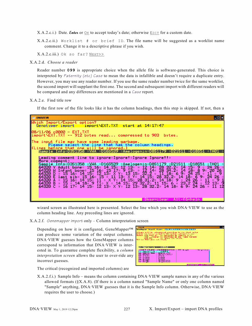
X.A.2.c.i.) Date. Enter or OK to accept today’s date; otherwise EDIT for a custom date.
X.A.2.c.ii.) Worklist # or brief ID. The file name will be suggested as a worklist name
comment. Change it to a descriptive phrase if you wish.
X.A.2.c.iii.) Ok so far? NEXT>>
X.A.2.d. Choose a reader
Reader number 099 is appropriate choice when the allele file is software-generated. This choice is
interpreted by Paternity (etc) Case to mean the data is infallible and doesn’t require a duplicate entry.
However, you may use any reader number. If you use the same reader number twice for the same worklist,
the second import will supplant the first one. The second and subsequent import with different readers will
be compared and any differences are mentioned in a Case report.
X.A.2.e. Find title row
If the first row of the file looks like it has the column headings, then this step is skipped. If not, then a
wizard screen as illustrated here is presented. Select the line which you wish DNA@VIEW to use as the
column heading line. Any preceding lines are ignored.
X.A.2.f. Genemapper import only – Column interpretation screen
Depending on how it is configured, GeneMapper™
can produce some variation of the output columns.
DNA@VIEW guesses how the GeneMapper columns
correspond to information that DNA@VIEW is inter-
ested in. To guarantee complete flexibility, a column
interpretation screen allows the user to over-ride any
incorrect guesses.
The critical (recognized and imported columns) are
X.A.2.f.i.) Sample Info – means the column containing DNA@VIEW sample names in any of the various
allowed formats (§X.A.8). (If there is a column named "Sample Name" or only one column named
"Sample" anything, DNA@VIEW guesses that it is the Sample Info column. Otherwise, DNA@VIEW
requires the user to choose.)
DNA@VIEW May 1, 2019 12:29pm X. Import/Export – import DNA profiles227
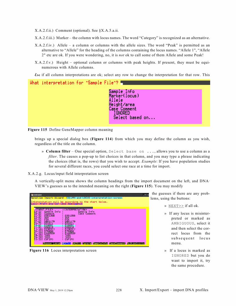
Figure 115 Define GeneMapper column meaning
Figure 116 Locus interpretation screen
X.A.2.f.ii.) Comment (optional). See §X.A.5.a.ii.
X.A.2.f.iii.) Marker – the column with locus names. The word “Category” is recognized as an alternative.
X.A.2.f.iv.) Allele – a column or columns with the allele sizes. The word “Peak” is permitted as an
alternative to “Allele” for the heading of the columns containing the locus names. “Allele 1", “Allele
2" etc are ok. If you were wondering, no, it is not ok to call some of them Allele and some Peak!
X.A.2.f.v.) Height – optional column or columns with peak heights. If present, they must be equi-
numerous with Allele columns.
Esc if all column interpretations are ok; select any row to change the interpretation for that row. This
brings up a special dialog box (Figure 114) from which you may define the column as you wish,
regardless of the title on the column.
» Column filter – One special option, Select base on ..., allows you to use a column as a
filter. The causes a pop-up to list choices in that column, and you may type a phrase indicating
the choices (that is, the rows) that you wish to accept. Example: If you have population studies
for several different races, you could select one race at a time for import.
X.A.2.g. Locus/input field interpretation screen
A vertically-split menu shows the column headings from the import document on the left, and DNAA
VIEW’s guesses as to the intended meaning on the right (Figure 115). You may modify
the guesses if there are any prob-
lems, using the buttons:
» NEXT>> if all ok.
» If any locus is misinter-
preted or marked as
AMBIGUOUS, select it
and then select the cor-
rect locus from the
s u b s e q u e n t l o c u s
menu.
» If a locus is marked as
IGNORED but you do
want to import it, try
the same procedure.
DNA@VIEW May 1, 2019 12:29pm X. Import/Export – import DNA profiles228
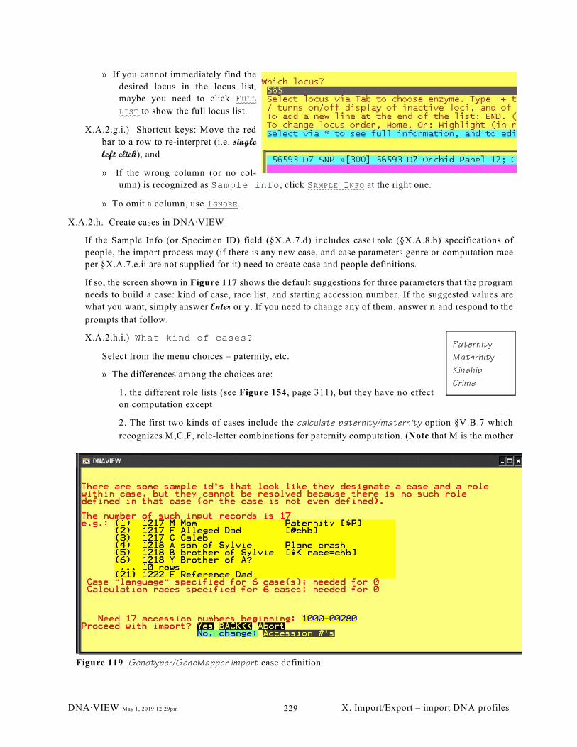
Paternity
Maternity
Kinship
Crime
Figure 119 Genotyper/GeneMapper import case definition
» If you cannot immediately find the
desired locus in the locus list,
maybe you need to click FULL
LIST to show the full locus list.
X.A.2.g.i.) Shortcut keys: Move the red
bar to a row to re-interpret (i.e. single
left click), and
» If the wrong column (or no col-
umn) is recognized as Sample info, click SAMPLE INFO at the right one.
» To omit a column, use IGNORE.
X.A.2.h. Create cases in DNAAVIEW
If the Sample Info (or Specimen ID) field (§X.A.7.d) includes case+role (§X.A.8.b) specifications of
people, the import process may (if there is any new case, and case parameters genre or computation race
per §X.A.7.e.ii are not supplied for it) need to create case and people definitions.
If so, the screen shown in Figure 117 shows the default suggestions for three parameters that the program
needs to build a case: kind of case, race list, and starting accession number. If the suggested values are
what you want, simply answer Enter or y. If you need to change any of them, answer n and respond to the
prompts that follow.
X.A.2.h.i.) What kind of cases?
Select from the menu choices – paternity, etc.
» The differences among the choices are:
1. the different role lists (see Figure 154, page 311), but they have no effect
on computation except
2. The first two kinds of cases include the calculate paternity/maternity option §V.B.7 which
recognizes M,C,F, role-letter combinations for paternity computation. (Note that M is the mother
DNA@VIEW May 1, 2019 12:29pm X. Import/Export – import DNA profiles229
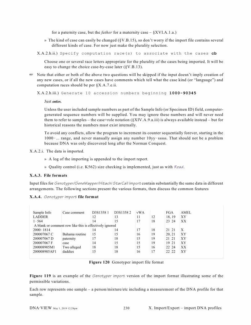
Sample Info Case comment D3S1358 1 D3S1358 2 vWA FGA AMELLADDER 12 13 11 12 18, 19 XY1!564 14 15 17 18 23 24 XX A blank or comment row like this is effectively ignored2000!1814 14 14 17 18 21 21 X200007067 C Bahama routine 15 15 16 19 20, 21 XY200007067 D paternity 17 18 15 19 21 21 XY200007067 F case 14 15 15 19 19 21 XY200008905M1 Two alleged 18 18 15 16 22 24 XX200008905AF1 daddies 15 18 16 17 22 22 XY
Figure 120 Genotyper import file format
for a paternity case, but the father for a maternity case – §XVI.A.1.a.)
» The kind of case can easily be changed (§V.B.15), so don’t worry if the import file contains several
different kinds of case. For now just make the plurality selection.
X.A.2.h.ii.) Specify computation race(s) to associate with the cases cb
Choose one or several race letters appropriate for the plurality of the cases being imported. It will be
easy to change the choice case-by-case later (§V.B.13).
L Note that either or both of the above two questions will be skipped if the input doesn’t imply creation of
any new cases, or if all the new cases have comments which tell what the case kind (or “language”) and
computation races should be per §X.A.7.e.ii.
X.A.2.h.iii.) Generate 10 accession numbers beginning 1000-90345
Just enter.
Unless the user included sample numbers as part of the Sample Info (or Specimen ID) field, computer-
generated sequence numbers will be supplied. You may ignore these numbers and will never need
them to refer to samples – the case+role notation (§XIV.A.9.a.iii) is always available instead – but for
historical reasons the numbers must exist internally.
To avoid any conflicts, allow the program to increment its counter sequentially forever, starting in the
1000!... range, and never manually assign any number 10yy!sssss. That should not be a problem
because DNA was only discovered long after the Norman Conquest.
X.A.2.i. The data is imported.
» A log of the importing is appended to the import report.
» Quality control (i.e. K562) size checking is implemented, just as with Read .
X.A.3. File formats
Input files for Genotyper/GeneMapper/Hitachi StarCall Import contain substantially the same data in different
arrangements. The following sections present the various formats, then discuss the common features
X.A.4. Genotyper import file format
Figure 119 is an example of the Genotyper import version of the import format illustrating some of the
permissible variations.
Each row represents one sample – a person/mixture/etc including a measurement of the DNA profile for that
sample.
DNA@VIEW May 1, 2019 12:29pm X. Import/Export – import DNA profiles230
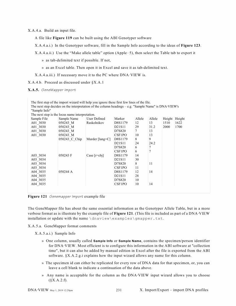
The first step of the import wizard will help you ignore these first few lines of the file.The next step decides on the interpretation of the column headings – e.g. "Sample Name" is DNA@VIEW's"Sample Info"The next step is the locus name interpretation.Sample File Sample Name User Defined Marker Allele Allele Height HeightA01_3030 050243_M Raskolnikov D8S1179 12 13 1510 1622A01_3030 050243_M D21S11 29 31.2 2000 1700A01_3030 050243_M D7S820 7 13A01_3030 050243_M CSF1PO 10 13
050243_C_Chip Murder [lang=C] D8S1179 8 9D21S11 24 24.2D7S820 6 7CSF1PO 6 7
A03_3034 050243 F Case [r=cbj] D8S1179 14A03_3034 D21S11 30A03_3034 D7S820 8 11A03_3034 CSF1PO 11A04_3035 050244 A D8S1179 12 14A04_3035 D21S11 28A04_3035 D7S820 10A04_3035 CSF1PO 10 14
Figure 121 Genemapper Import example file
X.A.4.a. Build an input file.
A file like Figure 119 can be built using the ABI Genotyper software
X.A.4.a.i.) In the Genotyper software, fill in the Sample Info according to the ideas of Figure 123.
X.A.4.a.ii.) Use the “Make allele table” option (Apple!5), then select the Table tab to export it
» as tab-delimited text if possible. If not,
» as an Excel table. Then open it in Excel and save it as tab-delimited text.
X.A.4.a.iii.) If necessary move it to the PC where DNA·VIEW is.
X.A.4.b. Proceed as discussed under §X.A.1
X.A.5. GeneMapper import
The GeneMapper file has about the same essential information as the Genotyper Allele Table, but in a more
verbose format as is illustrate by the example file of Figure 121. (This file is included as part of a DNA@VIEW
installation or update with the name \dnaview\examples\gmapper.txt.
X.A.5.a. GeneMapper format comments
X.A.5.a.i.) Sample Info
» One column, usually called Sample Info or Sample Name, contains the specimen/person identifier
for DNA@VIEW. Most efficient is to configure this information in the ABI software at "collection
time", but it can also be added by manual edition in Excel after the file is exported from the ABI
software. §X.A.2.g.i explains how the input wizard allows any name for this column.
» The specimen id can either be replicated for every row of DNA data for that specimen, or, you can
leave a cell blank to indicate a continuation of the data above.
» Any name is acceptable for the column as the DNA@VIEW input wizard allows you to choose
(§X.A.2.f).
DNA@VIEW May 1, 2019 12:29pm X. Import/Export – import DNA profiles231
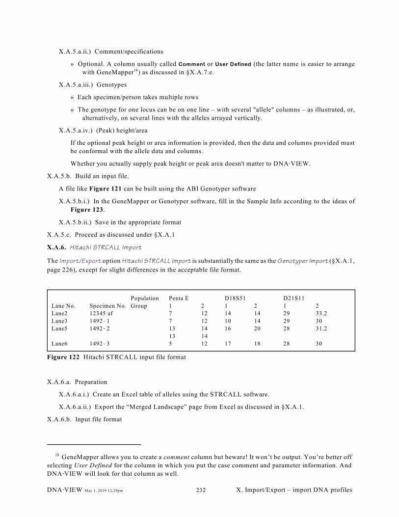
Population Penta E D18S51 D21S11
Lane No. Specimen No. Group 1 2 1 2 1 2
Lane2 12345 af 7 12 14 14 29 33.2
Lane3 1492!1 7 12 10 14 29 30
Lane5 1492!2 13 14 16 20 28 31.2
13 14
Lane6 1492!3 5 12 17 18 28 30
Figure 122 Hitachi STRCALL input file format
X.A.5.a.ii.) Comment/specifications
» Optional. A column usually called Comment or User Defined (the latter name is easier to arrange
with GeneMapper ) as discussed in §X.A.7.e.18
X.A.5.a.iii.) Genotypes
» Each specimen/person takes multiple rows
» The genotype for one locus can be on one line – with several "allele" columns – as illustrated, or,
alternatively, on several lines with the alleles arrayed vertically.
X.A.5.a.iv.) (Peak) height/area
If the optional peak height or area information is provided, then the data and columns provided must
be conformal with the allele data and columns.
Whether you actually supply peak height or peak area doesn't matter to DNA@VIEW.
X.A.5.b. Build an input file.
A file like Figure 121 can be built using the ABI Genotyper software
X.A.5.b.i.) In the GeneMapper or Genotyper software, fill in the Sample Info according to the ideas of
Figure 123.
X.A.5.b.ii.) Save in the appropriate format
X.A.5.c. Proceed as discussed under §X.A.1
X.A.6. Hitachi STRCALL Import
The Import/Export option Hitachi STRCALL import is substantially the same as the Genotyper Import (§X.A.1,
page 226), except for slight differences in the acceptable file format.
X.A.6.a. Preparation
X.A.6.a.i.) Create an Excel table of alleles using the STRCALL software.
X.A.6.a.ii.) Export the “Merged Landscape” page from Excel as discussed in §X.A.1.
X.A.6.b. Input file format
GeneMapper allows you to create a comment column but beware! It won’t be output. You’re better off18
selecting User Defined for the column in which you put the case comment and parameter information. And
DNA@VIEW will look for that column as well.
DNA@VIEW May 1, 2019 12:29pm X. Import/Export – import DNA profiles232
The input file is a tab-delimited text version of Hitachi’s “Merged Landscape”, as illustrated in Figure
122.
X.A.6.b.i.) Column headings
The column headings are arranged in a two-row format
» The locus names (Penta E, D18S51, etc.) are on the first line, and each of them is assumed
to apply to one (or more) columns to its right. The allele numbers, 1 and 2 in the second row, are
essentially ignored.
» The key word Lane No. in the second row designates the column containing the lane numbers.
» The key word Specimen in the second row designates a column with patient id information.
X.A.6.b.ii.) Data
» Each row of data must have a lane number such as Lane2 or Lane 2. (Unlabelled lanes can be,
according to Hitachi, either alternate assays of the same sample, or continuation lines containing
extra alleles. On an Excel spreadsheet the two possibilities are distinguished by colors, but since
DNA·VIEW has no way to tell which is which the line is ignored. Hand checking is therefore
advisable.)
» The Specimen Id information follows the same format and rules of interpretation as explained in
Figure 123, page 236.
X.A.6.c. Proceed as discussed under §X.A.1
X.A.7. File format details
X.A.7.a. Excel vs. Tab-delimited text
It depicts an Excel table, but since it must be converted to Tab-delimited text before it can be imported to
DNAAVIEW, the vertical lines really correspond to tab characters.
The allowable format is quite flexible.
X.A.7.b. Genotypes
The alleles for a locus can be entered
X.A.7.b.i.) in several columns, one allele per column the way the ABI Genotyper software does it, as
exemplified in the figure by D3S1358 and VWA.
To cater to mixtures, the number of columns is not limited.
X.A.7.b.ii.) in one column
» separated by space such as 23 24. They can also be separated by comma space, as 18, 19.
(Comma alone doesn’t work.) Note FGA in Figure 119. Any number of alleles are allowed.
» The space is not needed for SNP’s or other systems with 1-letter names like Amelogenin
An allele name like <10 or >22 is translated to 1 or 99.
X.A.7.b.iii.) Illegal alleles; important note: The treatment of an allele notation such as OL depends on
the OFFLADDER Options policy per §IX.F.25.
X.A.7.c. Locus column headings
DNA@VIEW May 1, 2019 12:29pm X. Import/Export – import DNA profiles233
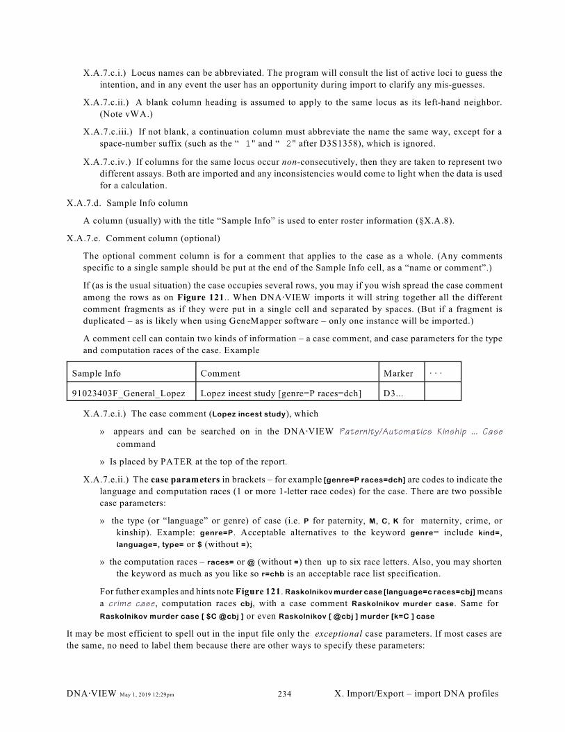
X.A.7.c.i.) Locus names can be abbreviated. The program will consult the list of active loci to guess the
intention, and in any event the user has an opportunity during import to clarify any mis-guesses.
X.A.7.c.ii.) A blank column heading is assumed to apply to the same locus as its left-hand neighbor.
(Note vWA.)
X.A.7.c.iii.) If not blank, a continuation column must abbreviate the name the same way, except for a
space-number suffix (such as the “ 1" and “ 2" after D3S1358), which is ignored.
X.A.7.c.iv.) If columns for the same locus occur non-consecutively, then they are taken to represent two
different assays. Both are imported and any inconsistencies would come to light when the data is used
for a calculation.
X.A.7.d. Sample Info column
A column (usually) with the title “Sample Info” is used to enter roster information (§X.A.8).
X.A.7.e. Comment column (optional)
The optional comment column is for a comment that applies to the case as a whole. (Any comments
specific to a single sample should be put at the end of the Sample Info cell, as a “name or comment”.)
If (as is the usual situation) the case occupies several rows, you may if you wish spread the case comment
among the rows as on Figure 121.. When DNA@VIEW imports it will string together all the different
comment fragments as if they were put in a single cell and separated by spaces. (But if a fragment is
duplicated – as is likely when using GeneMapper software – only one instance will be imported.)
A comment cell can contain two kinds of information – a case comment, and case parameters for the type
and computation races of the case. Example
Sample Info Comment Marker @ @ @
91023403F_General_Lopez Lopez incest study [genre=P races=dch] D3...
X.A.7.e.i.) The case comment (Lopez incest study), which
» appears and can be searched on in the DNA@VIEW Paternity/Automatics Kinship ... Case
command
» Is placed by PATER at the top of the report.
X.A.7.e.ii.) The case parameters in brackets – for example [genre=P races=dch] are codes to indicate the
language and computation races (1 or more 1-letter race codes) for the case. There are two possible
case parameters:
» the type (or “language” or genre) of case (i.e. P for paternity, M, C, K for maternity, crime, or
kinship). Example: genre=P. Acceptable alternatives to the keyword genre= include kind=,
language=, type= or $ (without =);
» the computation races – races= or @ (without =) then up to six race letters. Also, you may shorten
the keyword as much as you like so r=chb is an acceptable race list specification.
For futher examples and hints note Figure 121. Raskolnikov murder case [language=c races=cbj] means
a crime case, computation races cbj, with a case comment Raskolnikov murder case. Same for
Raskolnikov murder case [ $C @cbj ] or even Raskolnikov [ @cbj ] murder [k=C ] case
It may be most efficient to spell out in the input file only the exceptional case parameters. If most cases are
the same, no need to label them because there are other ways to specify these parameters:
DNA@VIEW May 1, 2019 12:29pm X. Import/Export – import DNA profiles234
» If omitted, the default values for the worklist/project are used – which the user may edit at the time
of input.
» Anyway the case parameters can be adjusted later, case-by-case, within the Paternity (etc) Case
program.
X.A.8. Defining the roster
The allowable Sample Info entries can be summarized by the notation:
{person-id}{case + role letter {description}},
where { } represent optional items. That is, the above notation means that any of the following options are
acceptable:
person-id
person-id case+role
person-id case+role description
case+role
case+role description
X.A.8.a. person-id – means a DNAAVIEW accession number (person number) with a dash in it, such as
2004-101,
X.A.8.b. case + role letter – means a case number followed by a role letter (upper or lower case ok). An
intervening space (or underscore – §X.A.8.d) is optional; either 4767C or 4767 C is ok. After the role
letter though please do put a space or underscore to separate it from any following description.
X.A.8.b.i.) role letter substitutions
In addition to the standard DNAAVIEW 1-letter roles such as C, D, E, ... for the first few children
in a paternity case, you may use C1, C2, C3, ... . Similarly you may put F1, F2, ... instead of
F, G, ..., and so on. Also, AF is acceptable instead of F.
X.A.8.c. description – Any text following the case+role letter is considered as a description for the person.
This can be the person’s name or any sample documentation. Up to 40 characters are accepted.
DNA@VIEW May 1, 2019 12:29pm X. Import/Export – import DNA profiles235
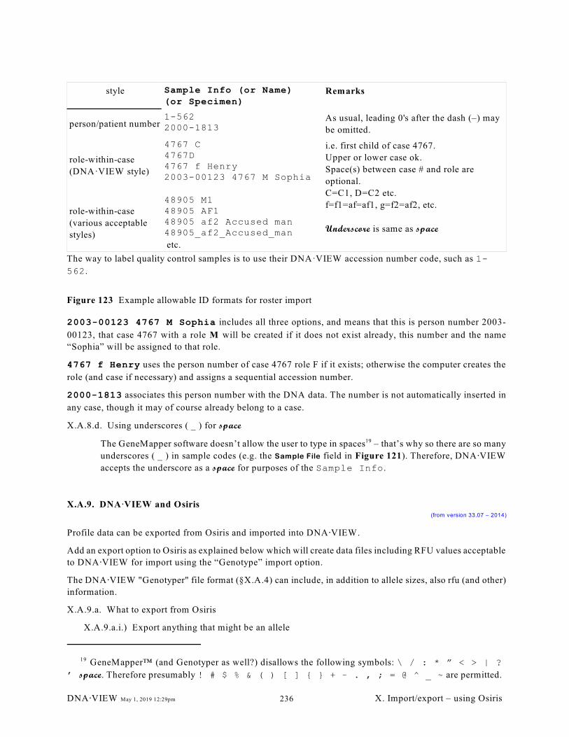
style Sample Info (or Name)(or Specimen)
Remarks
person/patient number1-5622000-1813
As usual, leading 0's after the dash (–) may
be omitted.
role-within-case
(DNA·VIEW style)
4767 C4767D 4767 f Henry2003-00123 4767 M Sophia
i.e. first child of case 4767.
Upper or lower case ok.
Space(s) between case # and role are
optional.
C=C1, D=C2 etc.
f=f1=af=af1, g=f2=af2, etc.
Underscore is same as space
role-within-case
(various acceptable
styles)
48905 M148905 AF148905 af2 Accused man48905_af2_Accused_man
etc.
The way to label quality control samples is to use their DNA·VIEW accession number code, such as 1-
562.
Figure 123 Example allowable ID formats for roster import
2003-00123 4767 M Sophia includes all three options, and means that this is person number 2003-
00123, that case 4767 with a role M will be created if it does not exist already, this number and the name
“Sophia” will be assigned to that role.
4767 f Henry uses the person number of case 4767 role F if it exists; otherwise the computer creates the
role (and case if necessary) and assigns a sequential accession number.
2000-1813 associates this person number with the DNA data. The number is not automatically inserted in
any case, though it may of course already belong to a case.
X.A.8.d. Using underscores ( _ ) for space
The GeneMapper software doesn’t allow the user to type in spaces – that’s why so there are so many19
underscores ( _ ) in sample codes (e.g. the Sample File field in Figure 121). Therefore, DNA@VIEW
accepts the underscore as a space for purposes of the Sample Info.
X.A.9. DNA@VIEW and Osiris(from version 33.07 – 2014)
Profile data can be exported from Osiris and imported into DNA@VIEW.
Add an export option to Osiris as explained below which will create data files including RFU values acceptable
to DNA@VIEW for import using the “Genotype” import option.
The DNA@VIEW "Genotyper" file format (§X.A.4) can include, in addition to allele sizes, also rfu (and other)
information.
X.A.9.a. What to export from Osiris
X.A.9.a.i.) Export anything that might be an allele
GeneMapper™ (and Genotyper as well?) disallows the following symbols: \ / : * ” < > | ?19
’ space. Therefore presumably ! # $ % & ( ) [ ] { } + ! . , ; = @ ^ _ ~ are permitted.
DNA@VIEW May 1, 2019 12:29pm X. Import/export – using Osiris236
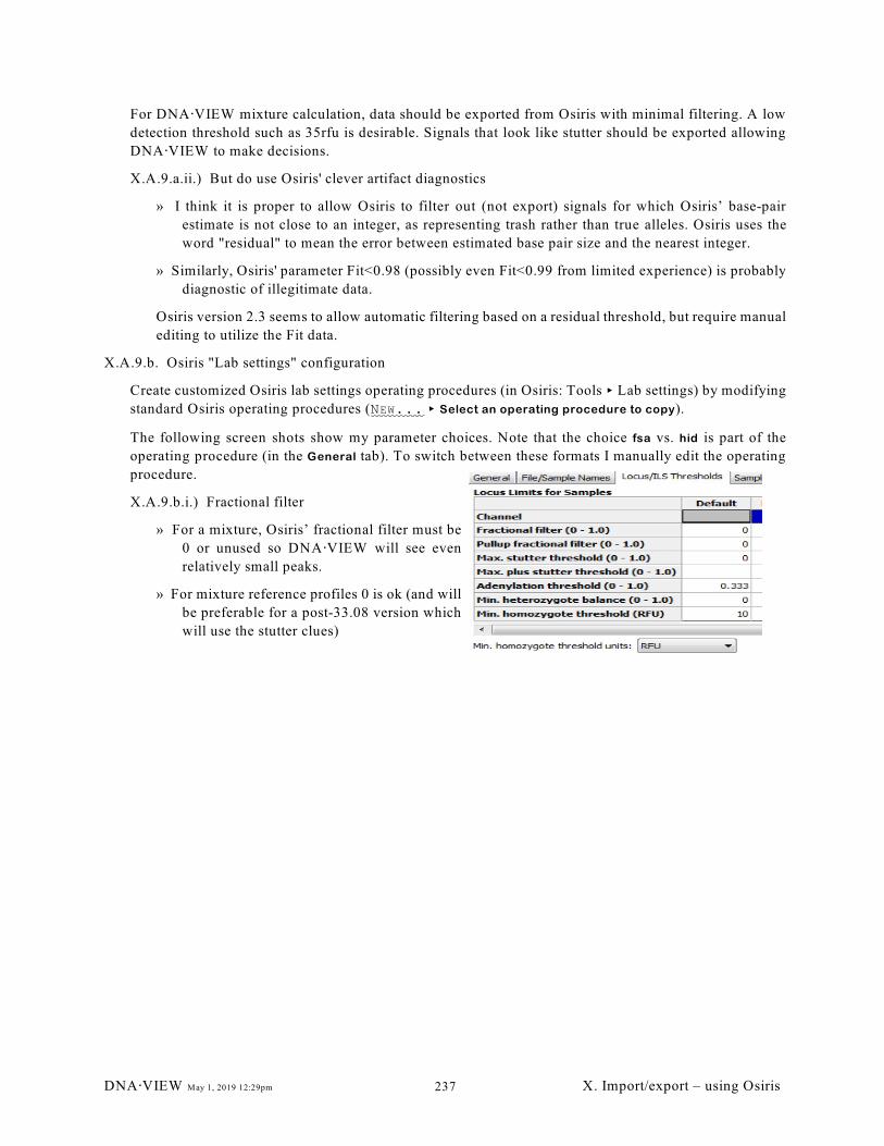
For DNA@VIEW mixture calculation, data should be exported from Osiris with minimal filtering. A low
detection threshold such as 35rfu is desirable. Signals that look like stutter should be exported allowing
DNA@VIEW to make decisions.
X.A.9.a.ii.) But do use Osiris' clever artifact diagnostics
» I think it is proper to allow Osiris to filter out (not export) signals for which Osiris’ base-pair
estimate is not close to an integer, as representing trash rather than true alleles. Osiris uses the
word "residual" to mean the error between estimated base pair size and the nearest integer.
» Similarly, Osiris' parameter Fit<0.98 (possibly even Fit<0.99 from limited experience) is probably
diagnostic of illegitimate data.
Osiris version 2.3 seems to allow automatic filtering based on a residual threshold, but require manual
editing to utilize the Fit data.
X.A.9.b. Osiris "Lab settings" configuration
Create customized Osiris lab settings operating procedures (in Osiris: Tools < Lab settings) by modifying
standard Osiris operating procedures (NEW... < Select an operating procedure to copy).
The following screen shots show my parameter choices. Note that the choice fsa vs. hid is part of the
operating procedure (in the General tab). To switch between these formats I manually edit the operating
procedure.
X.A.9.b.i.) Fractional filter
» For a mixture, Osiris’ fractional filter must be
0 or unused so DNA @VIEW will see even
relatively small peaks.
» For mixture reference profiles 0 is ok (and will
be preferable for a post-33.08 version which
will use the stutter clues)
DNA@VIEW May 1, 2019 12:29pm X. Import/export – using Osiris237
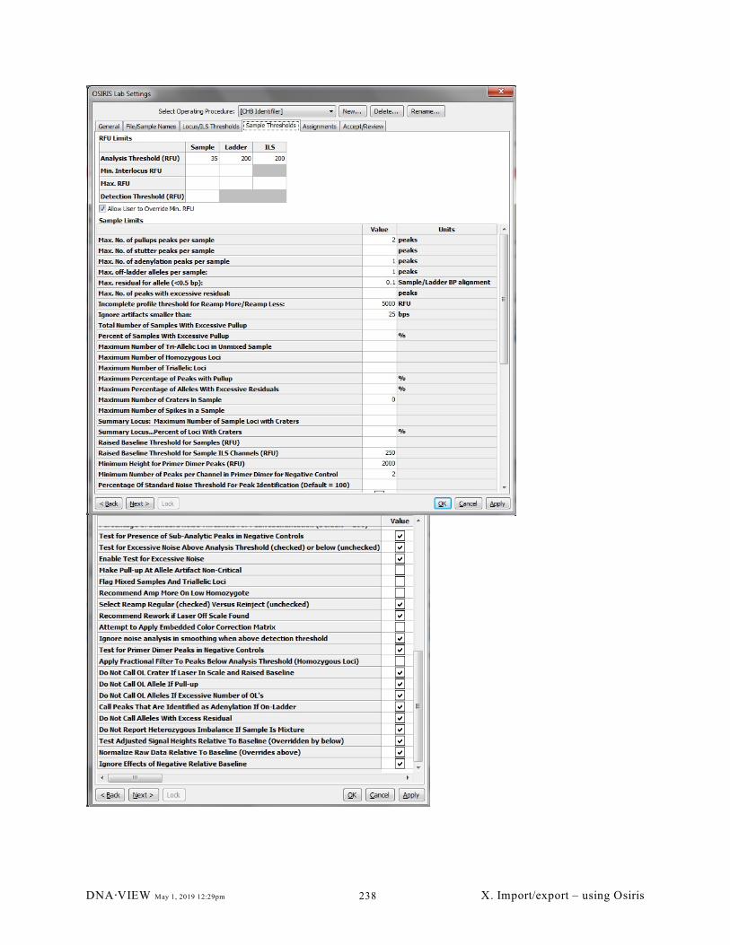
DNA@VIEW May 1, 2019 12:29pm X. Import/export – using Osiris238
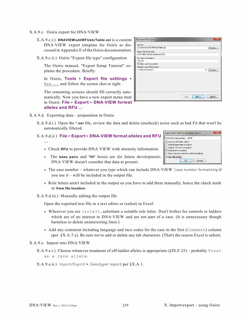
X.A.9.c. Osiris export for DNA@VIEW
X.A.9.c.i.) DNAVIEW\util\RFUetcTable.xsl is a custom
DNA @VIEW export template for Osiris as dis-
cussed in Appendix E of the Osiris documentation.
X.A.9.c.ii.) Osiris "Export file type" configuration
The Osiris manual, "Export Setup Tutorial" ex-
plains the procedure. Briefly:
In Osiris, Tools < Export file settings <
NEW... and follow the screen shot at right.
The remaining screens should fill correctly auto-
matically. Now you have a new export menu item
in Osiris: File < Export < DNA-VIEW format
alleles and RFU ...
X.A.9.d. Exporting data – preparation in Osiris
X.A.9.d.i.) Open the *.oer file, review the data and delete (uncheck) noise such as bad Fit that won't be
automatically filtered.
X.A.9.d.ii.) File < Export < DNA-VIEW format alleles and RFU
...
» Check RFU to provide DNA@VIEW with intensity information.
» The base pairs and "fit" boxes are for future development;
DNA@VIEW doesn't consider that data at present.
» The case number – whatever you type which can include DNA@VIEW Case number formatting if
you use it – will be included in the output file.
» Role letters aren't included in the output so you have to add them manually; hence the check mark
in View file location.
X.A.9.d.iii.) Manually editing the output file
Open the exported text file in a text editor or (safest) in Excel.
» Wherever you see (role?), substitute a suitable role letter. Don't bother for controls or ladders
which are of no interest to DNA@VIEW and are not part of a case. (It is unnecessary though
harmless to delete uninteresting lines.)
» Add any comment including language and race codes for the case in the first (Comment) column
(per §X.A.7.e). Be sure not to add or delete any tab characters. (That's the reason Excel is safest).
X.A.9.e. Import into DNA@VIEW
X.A.9.e.i.) Choose whatever treatment of off-ladder alleles is appropriate (§IX.F.25) – probably Treat
as a rare allele.
X.A.9.e.ii.) Import/Export < Genotyper import per §X.A.1.
DNA@VIEW May 1, 2019 12:29pm X. Import/export – using Osiris239
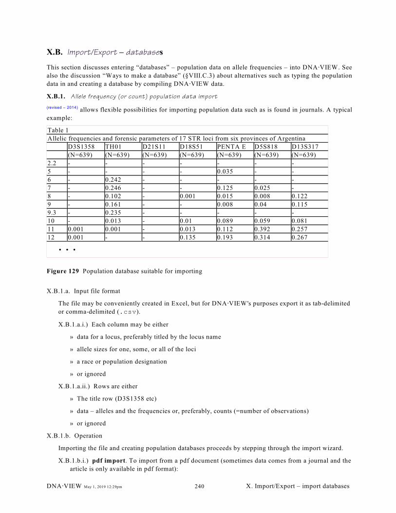
Table 1
Allelic frequencies and forensic parameters of 17 STR loci from six provinces of Argentina
D3S1358 TH01 D21S11 D18S51 PENTA E D5S818 D13S317
(N=639) (N=639) (N=639) (N=639) (N=639) (N=639) (N=639)
2.2 - - - - - - -
5 - - - - 0.035 - -
6 - 0.242 - - - - -
7 - 0.246 - - 0.125 0.025 -
8 - 0.102 - 0.001 0.015 0.008 0.122
9 - 0.161 - - 0.008 0.04 0.115
9.3 - 0.235 - - - - -
10 - 0.013 - 0.01 0.089 0.059 0.081
11 0.001 0.001 - 0.013 0.112 0.392 0.257
12 0.001 - - 0.135 0.193 0.314 0.267
@ @ @
Figure 129 Population database suitable for importing
X.B. Import/Export – databases
This section discusses entering “databases” – population data on allele frequencies – into DNA@VIEW. See
also the discussion “Ways to make a database” (§VIII.C.3) about alternatives such as typing the population
data in and creating a database by compiling DNA@VIEW data.
X.B.1. Allele frequency (or count) population data import
(revised – 2014) allows flexible possibilities for importing population data such as is found in journals. A typical
example:
X.B.1.a. Input file format
The file may be conveniently created in Excel, but for DNA@VIEW's purposes export it as tab-delimited
or comma-delimited (.csv).
X.B.1.a.i.) Each column may be either
» data for a locus, preferably titled by the locus name
» allele sizes for one, some, or all of the loci
» a race or population designation
» or ignored
X.B.1.a.ii.) Rows are either
» The title row (D3S1358 etc)
» data – alleles and the frequencies or, preferably, counts (=number of observations)
» or ignored
X.B.1.b. Operation
Importing the file and creating population databases proceeds by stepping through the import wizard.
X.B.1.b.i.) pdf import. To import from a pdf document (sometimes data comes from a journal and the
article is only available in pdf format):
DNA@VIEW May 1, 2019 12:29pm X. Import/Export – import databases240
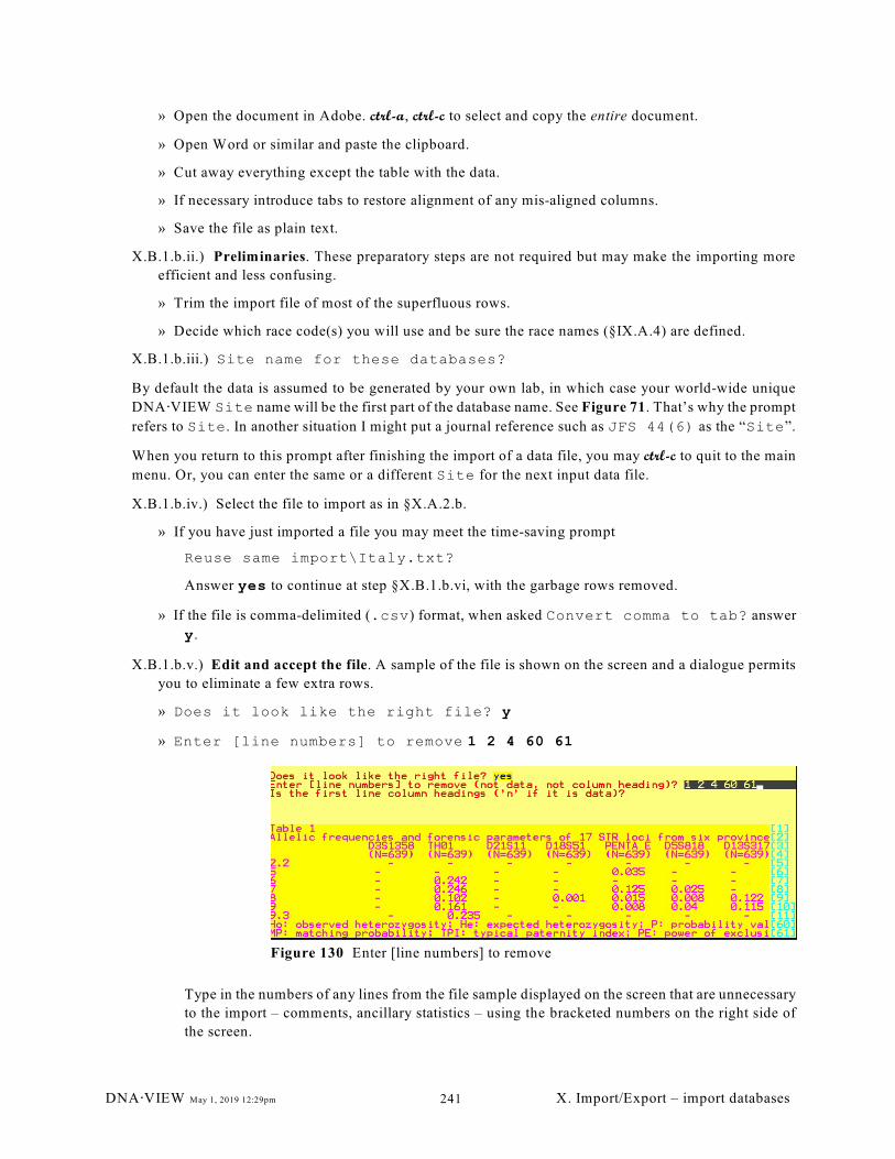
Figure 130 Enter [line numbers] to remove
» Open the document in Adobe. ctrl-a, ctrl-c to select and copy the entire document.
» Open Word or similar and paste the clipboard.
» Cut away everything except the table with the data.
» If necessary introduce tabs to restore alignment of any mis-aligned columns.
» Save the file as plain text.
X.B.1.b.ii.) Preliminaries. These preparatory steps are not required but may make the importing more
efficient and less confusing.
» Trim the import file of most of the superfluous rows.
» Decide which race code(s) you will use and be sure the race names (§IX.A.4) are defined.
X.B.1.b.iii.) Site name for these databases?
By default the data is assumed to be generated by your own lab, in which case your world-wide unique
DNA@VIEW Site name will be the first part of the database name. See Figure 71. That’s why the prompt
refers to Site. In another situation I might put a journal reference such as JFS 44(6) as the “Site”.
When you return to this prompt after finishing the import of a data file, you may ctrl-c to quit to the main
menu. Or, you can enter the same or a different Site for the next input data file.
X.B.1.b.iv.) Select the file to import as in §X.A.2.b.
» If you have just imported a file you may meet the time-saving prompt
Reuse same import\Italy.txt?
Answer yes to continue at step §X.B.1.b.vi, with the garbage rows removed.
» If the file is comma-delimited (.csv) format, when asked Convert comma to tab? answer
y.
X.B.1.b.v.) Edit and accept the file. A sample of the file is shown on the screen and a dialogue permits
you to eliminate a few extra rows.
» Does it look like the right file? y
» Enter [line numbers] to remove 1 2 4 60 61
Type in the numbers of any lines from the file sample displayed on the screen that are unnecessary
to the import – comments, ancillary statistics – using the bracketed numbers on the right side of
the screen.
DNA@VIEW May 1, 2019 12:29pm X. Import/Export – import databases241
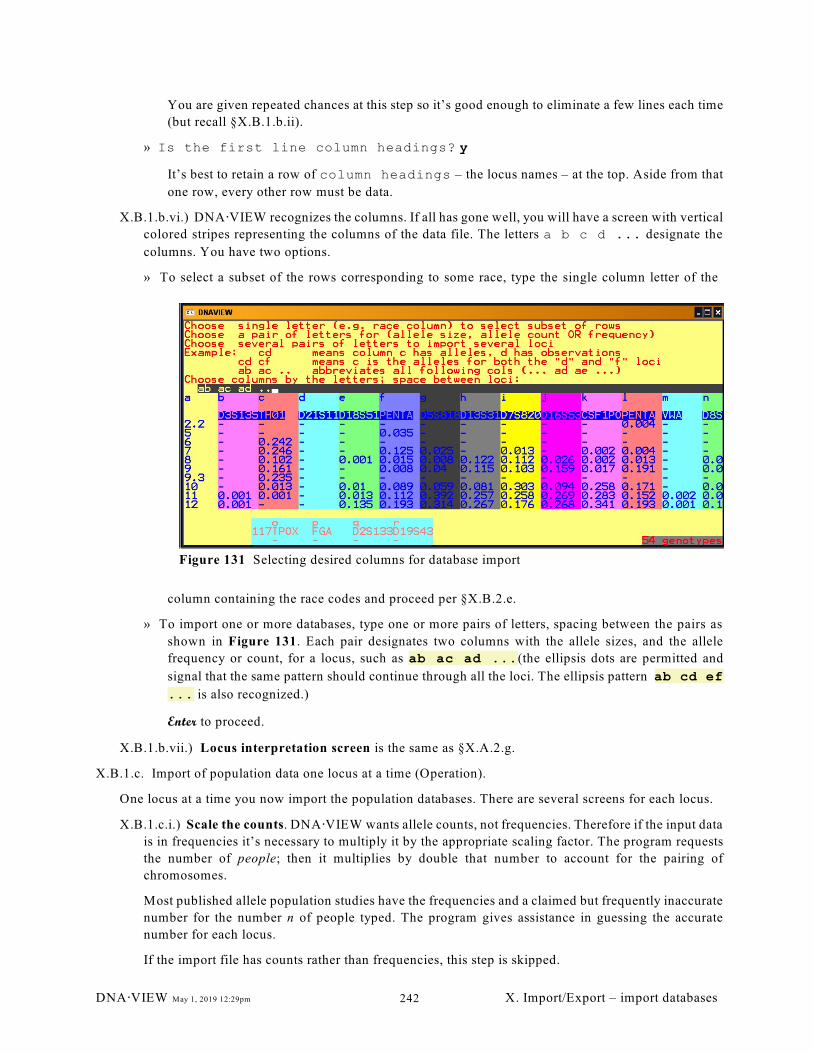
Figure 131 Selecting desired columns for database import
You are given repeated chances at this step so it’s good enough to eliminate a few lines each time
(but recall §X.B.1.b.ii).
» Is the first line column headings? y
It’s best to retain a row of column headings – the locus names – at the top. Aside from that
one row, every other row must be data.
X.B.1.b.vi.) DNA@VIEW recognizes the columns. If all has gone well, you will have a screen with vertical
colored stripes representing the columns of the data file. The letters a b c d ... designate the
columns. You have two options.
» To select a subset of the rows corresponding to some race, type the single column letter of the
column containing the race codes and proceed per §X.B.2.e.
» To import one or more databases, type one or more pairs of letters, spacing between the pairs as
shown in Figure 131. Each pair designates two columns with the allele sizes, and the allele
frequency or count, for a locus, such as ab ac ad ...(the ellipsis dots are permitted and
signal that the same pattern should continue through all the loci. The ellipsis pattern ab cd ef
... is also recognized.)
Enter to proceed.
X.B.1.b.vii.) Locus interpretation screen is the same as §X.A.2.g.
X.B.1.c. Import of population data one locus at a time (Operation).
One locus at a time you now import the population databases. There are several screens for each locus.
X.B.1.c.i.) Scale the counts. DNA@VIEW wants allele counts, not frequencies. Therefore if the input data
is in frequencies it’s necessary to multiply it by the appropriate scaling factor. The program requests
the number of people; then it multiplies by double that number to account for the pairing of
chromosomes.
Most published allele population studies have the frequencies and a claimed but frequently inaccurate
number for the number n of people typed. The program gives assistance in guessing the accurate
number for each locus.
If the import file has counts rather than frequencies, this step is skipped.
DNA@VIEW May 1, 2019 12:29pm X. Import/Export – import databases242
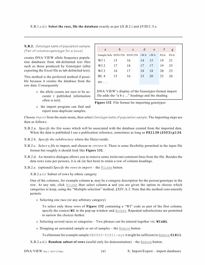
a b c d e f g
Sample Info D3S1358 D3S1358 vWA vWA FGA FGA
WI 1 15 16 14 15 19 21
WI 2 17 18 17 17 19 25
WI 3 16 17 18 18 20 23
BL 4 15 16 15 20 23 26
etc . . .
DNA·VIEW’s display of the Genotyper-format import
file adds the “a b c ...” headings and the shading.
Figure 132 File format for importing genotypes
X.B.1.c.ii.) Select the race, file the database exactly as per §X.B.2.i and §VIII.C.5.e.
X.B.2. Genotype table of population sample.
(Pair of columns=genotype for a locus)
creates DNA·VIEW allele frequency popula-
tion databases from tab-delimited text files
such as those produced by Genotyper (after
exporting the Excel file as tab-delimited text).
This method is the preferred method if possi-
ble because it creates the database from the
raw data. Consequently
» the allele counts are sure to be ac-
curate ( published information
often is not);
» the import program can find and
report near-duplicate samples.
Choose Import from the main menu, then select Genotype table of population sample. The importing steps are
then as follows:
X.B.2.a. Specify the Site name which will be associated with the database created from the imported data.
When the data is published I use a publication reference, sometimes as long as FSI138(2003)p134.
X.B.2.b. Specify the subdirectory where the file(s) reside.
X.B.2.c. Select a file to import, and choose to retrieve it. There is some flexibility permitted in the input file
format but roughly it should look like Figure 132.
X.B.2.d. An iterative dialogue allows you to remove some irrelevant comment lines from the file. Besides the
data rows (one per person), it is ok (in fact best) to retain a row of column headings.
X.B.2.e. (optional) Specify the rows to import – the FILTER button.
X.B.2.e.i.) Subset of rows by ethnic category
One of the columns, for example column a, may be a category description for the person/genotype in the
row. At any rate, click FILTER then select column a and you are given the option to choose which
categories to keep, using the “Multiple selection” method, §XIV.A.3. Note that the method conveniently
permits
» Selecting one race (or any arbitrary category)
To select only those rows of Figure 132 containing a “WI” code as part of the first column,
specify the context WI in the pop-up window and ACCEPT. Repeated subselections are permitted
to narrow the choices further.
» Selecting several races or categories – Two phrases can be entered together vis: WI&BL
» Dropping an unwanted sample or set of samples – the REMOVE button.
To eliminate for example sample DB2003-01811-xyz it might be sufficient to REMOVE 01811.
X.B.2.e.ii.) Random subset of rows (useful only for demonstration) – the RANDOM button.
DNA@VIEW May 1, 2019 12:29pm X. Import/Export – import databases243
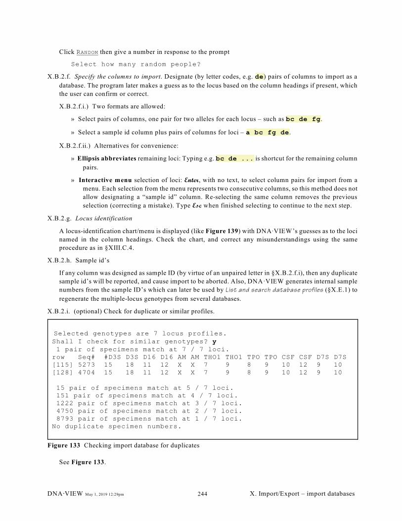
Selected genotypes are 7 locus profiles.Shall I check for similar genotypes? y 1 pair of specimens match at 7 / 7 loci.row Seq# #D3S D3S D16 D16 AM AM THO1 THO1 TPO TPO CSF CSF D7S D7S[115] 5273 15 18 11 12 X X 7 9 8 9 10 12 9 10[128] 4704 15 18 11 12 X X 7 9 8 9 10 12 9 10
15 pair of specimens match at 5 / 7 loci. 151 pair of specimens match at 4 / 7 loci. 1222 pair of specimens match at 3 / 7 loci. 4750 pair of specimens match at 2 / 7 loci. 8793 pair of specimens match at 1 / 7 loci.No duplicate specimen numbers.
Figure 133 Checking import database for duplicates
Click RANDOM then give a number in response to the prompt
Select how many random people?
X.B.2.f. Specify the columns to import. Designate (by letter codes, e.g. de) pairs of columns to import as a
database. The program later makes a guess as to the locus based on the column headings if present, which
the user can confirm or correct.
X.B.2.f.i.) Two formats are allowed:
» Select pairs of columns, one pair for two alleles for each locus – such as bc de fg.
» Select a sample id column plus pairs of columns for loci – a bc fg de.
X.B.2.f.ii.) Alternatives for convenience:
» Ellipsis abbreviates remaining loci: Typing e.g. bc de ... is shortcut for the remaining column
pairs.
» Interactive menu selection of loci: Enter, with no text, to select column pairs for import from a
menu. Each selection from the menu represents two consecutive columns, so this method does not
allow designating a “sample id” column. Re-selecting the same column removes the previous
selection (correcting a mistake). Type Esc when finished selecting to continue to the next step.
X.B.2.g. Locus identification
A locus-identification chart/menu is displayed (like Figure 139) with DNAAVIEW’s guesses as to the loci
named in the column headings. Check the chart, and correct any misunderstandings using the same
procedure as in §XIII.C.4.
X.B.2.h. Sample id’s
If any column was designed as sample ID (by virtue of an unpaired letter in §X.B.2.f.i), then any duplicate
sample id’s will be reported, and cause import to be aborted. Also, DNA·VIEW generates internal sample
numbers from the sample ID’s which can later be used by List and search database profiles (§X.E.1) to
regenerate the multiple-locus genotypes from several databases.
X.B.2.i. (optional) Check for duplicate or similar profiles.
See Figure 133.
DNA@VIEW May 1, 2019 12:29pm X. Import/Export – import databases244
X.B.2.j. Iteratively per locus, create a database.
X.B.2.j.i.) Choose the race letter to be associated with the database.
X.B.2.j.ii.) File the database (or skip it) as explained in §VIII.C.5.e.
X.C.
DNA@VIEW May 1, 2019 12:29pm X. Import/Export – import databases245
Import/Export – sharing databases
Two complementary facilities to allow users to swap databases are described below.
X.C.1. DNA@VIEW Frequency Database Import (transfer between users)
The Import/Export option DNA@VIEW frequency database import lets you integrate additional, DNA·VIEW
supplied databases into your list of databases.
The new databases may be supplied on a disk, with a filename such as DNAFREQ.SF, but in any case with
the extension .SF. The file can either be the \dnaview\dnafreq.sf file of a DNAAVIEW system, or can
be a file created by the complementary Export DNA@VIEW databases (§X.C.2) facility.
You can copy the file to your hard disk for faster operation if you like, but be sure not to overwrite the
DNAFREQ.SF file that contains your current list. Either copy it to another subdirectory, or change the name,
e.g. to NEWFREQ.SF. The extension must be SF.
Also, you can Import from your Demo system (§XI.E) to populate an empty Production system list of data
bases.
X.C.1.a. Select file from which to import
The command first queries for the path and name of the new file.
X.C.1.b. Mass selection of databases to import
Then you are given the opportunity to limit the list of possible databases to import using the “mass
selection” method as described in §XIV.A.3. It is often convenient to enter, temporarily selecting all of
them; you will later get the chance to narrow the selection.
X.C.1.c. The import process iterates through the remaining choices one at a time.
X.C.1.c.i.) Each new database that is identical to an old one is skipped.
X.C.1.c.ii.) Otherwise, the directory entry for the new database is shown and you are asked Import?.
X.C.1.c.iii.) n if you don’t want it. Then you will again be presented with the remaining list of databases
to import, so you can narrow that list systematically. For example – offer & rejection:
I can import: (# 30 / 996 ) Import it? nD3S1358 STR Canada CFS East Indian 167 01/09/21 1 pm
Helpful offer:
Limit databases again if desiredAccept lines containing ~ 966 databases
To reject similar database quickly:
Accept lines containing ~CFS enter 958 databases
X.C.1.d. y to (probably) import the new database
The imported database can either be added to your collection, or can update a database already there.
You are presented with a list of candidates for replacement — same probe and same race(s).
» Press End to make a new entry, or
» select one of the old entries to replace it.
DNA@VIEW May 1, 2019 12:29pm X. Import/Export – swap databases246
In the case of replacing an old entry, the program will display both the new database and the
candidate for replacement side-by-side, and ask for further confirmation before making the
replacement, as shown in Figure 79, page 165.
After completing the import, you may wish to use Database < Set default database, per race (§VIII.C.2.b,
page 160) to check that the default race selections are as intended.
X.C.2. Export DNA@VIEW databases (transfer between users)
Export DNA@VIEW databases is the inverse of DNA@VIEW frequency data import (§X.B).
You are first asked
Subdirectory for the DNAFREQ.SF file to export to?
You may choose for example A:, if you have a good diskette in drive A.
File name: Usually choose (new file) from the menu.
Then File name? Supply a DOS file prefix (no dot); the system will add the .SF suffix.
The rest of the operation is similar to importing – multiple selection (§XIV.A.3) to get the approximate list
of databases to transfer, then prompting for each possible choice.
X.D. Import/Export – GeneScan & Pharmacia
This chapter on options for importing data by migration amount and having DNA@VIEW compute the size and
allele calls has been removed for space. If you are interested older manuals are available on-line.
X.E. Import/Export – miscellaneous options
X.E.1. List and search database profiles
This Import/Export option includes several possibilities.
X.E.1.a. List database profiles
Produce a list of phenotypes obtained from one or several databases. If the databases each contain
substantially the same people typed in different probes then the list will show the multiple-locus phenotype
for each person. It is only possible with DNA@VIEW-compiled databases (§VIII.C.5, §VIII.C.7).
X.E.1.b. Search for matching profiles
You may also ask the program to make a special search for partly or completely similar profiles. You may
X.E.1.b.i.) search the entire database for duplicates (or, if RFLP, near-duplicates),
X.E.1.b.ii.) search the entire database against one or a few specific profiles. This search can be either for
full-profile match, or for half-match (one allele at each locus, such as parent and child).
The specific profiles can be
» profiles previously entered into DNA@VIEW, specified by accession ID, AND/OR
DNA@VIEW May 1, 2019 12:29pm X. Import/Export – duplicate phenotypes247
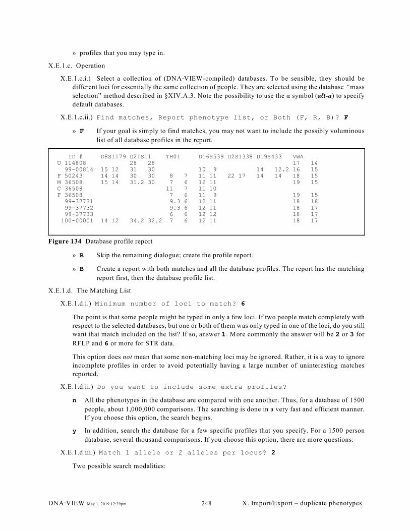
ID # D8S1179 D21S11 TH01 D16S539 D2S1338 D19S433 VWA U 114808 28 28 17 14 99-00814 15 12 31 30 10 9 14 12.2 16 15 F 50243 14 14 30 30 8 7 11 11 22 17 14 14 18 15 M 36508 15 14 31.2 30 7 6 12 11 19 15 C 36508 11 7 11 10 F 36508 7 6 11 9 19 15 99-37731 9.3 6 12 11 18 18 99-37732 9.3 6 12 11 18 17 99-37733 6 6 12 12 18 17 100-00001 14 12 34.2 32.2 7 6 12 11 18 17
Figure 134 Database profile report
» profiles that you may type in.
X.E.1.c. Operation
X.E.1.c.i.) Select a collection of (DNA@VIEW-compiled) databases. To be sensible, they should be
different loci for essentially the same collection of people. They are selected using the database “mass
selection” method described in §XIV.A.3. Note the possibility to use the á symbol (alt-a) to specify
default databases.
X.E.1.c.ii.) Find matches, Report phenotype list, or Both (F, R, B)? F
» F If your goal is simply to find matches, you may not want to include the possibly voluminous
list of all database profiles in the report.
» R Skip the remaining dialogue; create the profile report.
» B Create a report with both matches and all the database profiles. The report has the matching
report first, then the database profile list.
X.E.1.d. The Matching List
X.E.1.d.i.) Minimum number of loci to match? 6
The point is that some people might be typed in only a few loci. If two people match completely with
respect to the selected databases, but one or both of them was only typed in one of the loci, do you still
want that match included on the list? If so, answer 1. More commonly the answer will be 2 or 3 for
RFLP and 6 or more for STR data.
This option does not mean that some non-matching loci may be ignored. Rather, it is a way to ignore
incomplete profiles in order to avoid potentially having a large number of uninteresting matches
reported.
X.E.1.d.ii.) Do you want to include some extra profiles?
n All the phenotypes in the database are compared with one another. Thus, for a database of 1500
people, about 1,000,000 comparisons. The searching is done in a very fast and efficient manner.
If you choose this option, the search begins.
y In addition, search the database for a few specific profiles that you specify. For a 1500 person
database, several thousand comparisons. If you choose this option, there are more questions:
X.E.1.d.iii.) Match 1 allele or 2 alleles per locus? 2
Two possible search modalities:
DNA@VIEW May 1, 2019 12:29pm X. Import/Export – duplicate phenotypes248
1 for a “Paternity search” — people sharing one allele at each locus. If you choose this option the
search will only database vs. entered profiles – there is no database vs. database paternity
search.
2 “Full search” looks for people matching both alleles at each locus. It compares all profiles in the
databases with one another, as well with any extra profiles.
X.E.1.d.iv.) Accession # to match?
Profiles that already exist in DNA@VIEW can easily be chosen using their accession # or role+case
(per §XIV.A.9.a.iii). Choose as many, one at a time, as you wish.
Simply enter accepting the “year” number of 0 number to finish.
X.E.1.d.v.) Would you like to type in some profiles? n
This is less convenient, but gives you the chance to search for anything and also to edit/modify and
profiles specified in the previous step.
The editing format is two lines per person, one column per locus (because there are two sizes at each
locus). Example:
[0] YNH [1] TBQ[0] 93-12345 [0] 1234 2345[1] 93-12345 [1] 0 3000[2] Person 1 [2] 1234 2345[2] Person 1 [3] 2000 3000
will find anyone in the databases that matches (2345 3000) in TBQ, and matches either homozygous
1234 or (1234 2000) in YNH. Data entry is using the numeric editor (XIV.B.2.b). Allele notation is
allowed. Ctrl-e when finished.
X.E.1.d.vi.) Example of a matching list
Matching pairs are listed with a score (0.0 = exact match). Example:
[0] [1] [2] [3] [4] [5] ID # D8S1179 D21S11 TH01 D16S539 D2S1338 VWAAverage std dev diff/band=0.0 Maximum=0.0 U 185 15 13 33.2 32.2 9.3 7 14 11 25 17 16 15 F 185 33.2 32.2 9.3 7 14 11 25 17
Average std dev diff/band=0.0 Maximum=0.0 1001-02599 15 14 30.2 29 9.3 8 11 9 19 15 2007-83838 15 14 19 15
For RFLP searches there are some additional options and parameters. Find an archived old version of this
manual if you are interested.
X.E.1.e. Database searching and convicted offenders or missing persons
Three possible methods:
X.E.1.e.i.) A high-powered searching facility Search NDIS for Relatives that allows a database of
unlimited size and implements not only direct searching but also kinship searching is under
development, and will be an extra-cost option.
As currently envisioned it's use is limited to searching and it is not intended for cataloguing offenders
nor offender list maintenance.
DNA@VIEW May 1, 2019 12:29pm X. Import/Export – duplicate phenotypes249
X.E.1.e.ii.) The Screen disaster matches command can be used in the same way but limited to about
100,000 offenders.
X.E.1.e.iii.) The searching method described above for DNA@VIEW compiled databases can be used to
maintain offender lists and search for direct matches, for a limited number of offenders. The protocol
would involve setting up appropriate DNA·VIEW databases, updating them as necessary, and using
the above List and search database profiles (§X.E.1) facility to search. The database maintenance
protocol is laid out in detail in §VIII.C.4.
The search then proceeds. Print or File < Save as the result report.
X.E.2. LIMS import of case & person definitions
Import file specifications are on the web at http://dna-view.com/interface.htm. Accepts text files defining cases
and people.
X.E.3. Case and accession data import
This is an old and unused facility. See an older manual for documentation. Contact the DNA@VIEW author for
newer and more comprehensive approaches to DNA@VIEW – LIMS integration.
X.F. CODIS: export size data in CMF format
This rarely referenced section has been removed to save paper. Consult a pre-2007 manuals, available on-line,
if interested.
X.G. Integration of DNA•VIEW within LIMS system
Some of the features of DNAAVIEW can be controlled by a script, which permits using DNAAVIEW as an
engine under the control of a LIMS systems. The LIMS creates certain files – a genotyper table with DNA
profiles, a script file instructing DNAAVIEW to do certain operations such as read in the DNA data, make
paternity calculations, kinship calculations, or kinship simulations. Eventually DNAAVIEW signals completion
and stops. Then the results can be collected by the LIMS system and integrated into its database.
As of now establishing the LIMS–DNAAVIEW link is a custom task; i.e. some consulting is involved.
DNA@VIEW May 1, 2019 12:29pm X. Import/Export – LIMS integration250
XI. PROGRAM VALIDATION & MAINTENANCE
XI.A. Program Validation
Program validation means assuring that the program does what it should. Some aspects of validation:
§XI.A.1 lists some test suites built into DNA@VIEW.
§XI.A.2 lists facilities in DNA@VIEW to document standard settings and detect accidental tampering.
§XI.A.3 suggests a protocol for validation by checking user cases.
§VI.F.8 can be helpful to compare against a published case.
§XI.A.4 discusses database validation.
XI.A.1. Test suites in DNA@VIEW
The tests in this section were mainly written for the program developer, but are available for the user to run
also. They validate by comparing operation of the program against canned results, or against a calculation
using a different algorithm. In that way they test whether a program error has been introduced.
XI.A.1.a. Paternity and maternity case calculations (§V.B.30)
Casework < Parentage Case < (CALCULATE button) parentage test examples
Runs a suite (or selected example) of one-locus calculations covering examples of maternity, paternity,
duo, trio, mutation, and silent alleles.
XI.A.1.b. Kinship test examples (§VI.K.9)
Casework < Prototype Kinship < run test cases; check program
Derives the formulas for a suite of kinship problem and compares them with canned results.
XI.A.1.c. Mixture formula testing
The DNA@VIEW Mixture Solution – the LR method one (§V.D) – includes two completely different
algorithms for deriving the LR formula, so they can be used to test one another. There is a set of canned
examples, and you can also test your own examples.
XI.A.1.c.i.) Mixture test suite (§V.D.9)
Casework < Automatic mixture < (CALCULATE button) mixture examples
XI.A.1.c.ii.) Roll your own
Open any of your mixture cases and proceed to the Locus mixture computation screen (?) for some
locus. Set è=0 and observe the LR formula and value. Then set è=0.00001, which will trigger the
DNA@VIEW May 1, 2019 12:29pm XI. Program Maintenance – Import/export251
alternative, è-sensitive, algorithm. The formula will look a little different because of the incidence of
all the T’s (which represent è), but with è so small the numerical LR should be identical.
XI.A.1.d. Kinship simulation test case
This one may a little inconvenient for users, as it assumes the reference database for race c is the JFS 44(6)
CODIS Caucasian Profiler+ & Cofiler population data. It also may be unimportant.
Casework < Open Case < select any case < simulation menu < (SIMULATE button) Run test case
XI.A.2. Facilities for documenting DNA@VIEW settings
XI.A.2.a. Report parameter etc. settings in DNA@VIEW
including default databases and mutation rates, use §IX.A.11, Housekeeping < Maintenance < report
systemwide switch/parameter settings.
XI.A.2.b. Warn of changed parameter settings.
Under Housekeeping < Maintenance, see §IX.A.13 compare and §IX.A.12 record switch/parameter
settings.
XI.A.3. Protocol for casework validation
Many labs like to check after a software update that the new version will give expected results, or at least
to see and understand any differences from the previous version. For that purpose it’s convenient to have
a handful of test cases. I suggest choosing from the lab’s actual casework some cases covering a variety
of situations that are part of the lab’s normal work, i.e. paternity including inclusion, exclusion, mutation,
etc.; kinship; mixture.
XI.A.3.a.i.) Tagging the validation cases
I give each validation case a comment (§V.B.11 edit case comment) including a distinctive code such as
$v. This (arbitrary) code is convenient in conjunction with Open case. As per §V.B.28.a.ii, it makes it
quick to find all of them and to open one at a time for testing.
XI.A.3.a.ii.) Record the kinship scenario
For kinship validation cases, especially if the kinship scenario is complicated use the “pick list” (§VI.F.7.p
Scenario from/to pick list) to save it. Include the case number and perhaps $v as comment in the scenario.
That makes it easier to find the scenario when using the FETCH FROM PICKLIST button (§VI.F.1.a.i).
XI.A.3.a.iii.) Record the right answer
In a comment field – either the case comment or, if a kinship case as a comment in the pick list scenario
– make a note of the calculation conditions (what reference databases) and the desired answer (LR= for
the various races calculated).
Once the validations cases are nicely set up, checking five or ten cases takes only a few minutes.
XI.A.4. Database validation
One possible and possibly useful meaning of database validation is supplied by the Database similarity test
of §VIII.I. More traditional but of more dubious value is checking for Hardy-Weinberg equilibrium etc – see
§VIII.G Exact Tests for Independence.
DNA@VIEW May 1, 2019 12:29pm XI. Program Maintenance – Import/export252
XI.B. Update
The Update command is used to complete installation (or possibly repair) of a new (or repaired) version of
DNA·VIEW. In those circumstances Update starts automatically; no need for the user to invoke it. It does
though ask permission to run:
Ok to proceed with software update? answer YES.
Improvements and modifications to DNAAVIEW consist of an update installer CD, or download. After you
run the installer (as explained in §XV.A, Installation Appendix) DNA@VIEW will only present a reduced menu
of commands until the Update process is permitted to run. Update makes some data file changes so that your
data files will become compatible with the new DNA@VIEW program release.
(The update files have been copied into the \DNAVIEW\UPDATES directory by INSTALL as part of the
update installation. Once the Update has been performed those files are no longer necessary.)
XI.C. Program Errors
Despite the greatest care in preparation and testing, programs inevitably have errors. We need your help with
both of these kinds:
XI.C.1. Wrong answers
These can come from algorithmic errors in the programs, or from errors in the tables. Our only possible
protection against these is vigilance. Spot check the output for plausibility. Be especially watchful when you
get a new version of the program.
XI.C.2. Fatal errors
These are error conditions detected by the program itself, and which prevent it from continuing.
Conceivably you can generate one by an unanticipated data entry error — maybe a fractional case number.
In such a case the program will stop with a message including wording like VALUE ERROR, SYNTAX
ERROR, or DISK FULL. It will also print a fax form.
XI.C.2.a. Reporting errors
Please report errors, both to help yourself and because this is one way that DNA@VIEW is in a constant state
of improvement.
There are two good ways to report an error –
XI.C.2.a.i.) Send or fax the fax. Please include a contact phone number. At the time of the error the
program will wait at a special prompt; sometimes I need to ask you to try some experiments at the
point of this prompt to further diagnose the problem. Therefore, if it is convenient for you to leave the
computer in its exact state and contact me immediately, please do so.
XI.C.2.a.ii.) Email the DNAERROR.SF file (from the DNAVIEW\ main folder). This file contains all the
information that the fax does provided that you have not answered yet affirmatively to the sign-off
prompt Have you sent off the error report from May 6 yet? The point is that
when you answer y the error file is erased and the diagnostic information is therefore lost.
DNA@VIEW May 1, 2019 12:29pm XI. Program Maintenance253
XI.C.2.b. Recovering from errors
Here are some procedures that will sometimes get you past such a problem:
XI.C.2.b.i.) For some errors the error report will include a suggested remedy. Try it.
XI.C.2.b.ii.) Turn the computer off and back on again. Sometimes a computer gets into a strange state.
XI.C.2.b.iii.) Try looking at the data in a different way. If you can determine that some part of it is
peculiar, try deleting that part.
XI.C.3. Network lock
Occasionally a networked DNA@VIEW system runs into a Paradox interlock problem. The symptom is either
a red Waiting for table box on the screen that won’t go away, or an error starting DNA@VIEW that refers to
Paradox.
The cure is to sign everybody off of DNA@VIEW and PATER, invoke the Repair tool (§XI.G) from the desktop
icon, and choose the Fix option.
XI.D. DNA·VIEW Files
XI.D.1. Data files
XI.D.1.a. DNACFG.SF contains vital configuration information.
In case of an individualized network configuration, in addition to the master DNACFG.SF on the (shared)
server, there may also be a local copy for an individual workstation. This allows the separate workstations
to refer to different printers, and to maintain different values of certain preserved settings such as the last
DNA odds calculation.
In addition, there may be a copy of this file in the UPDATES\ folder. That file is only needed temporarily
during update to a new DNA@VIEW (or PATER) version.
XI.D.1.b. DNAMAINT.SF contains configuration information mainly about loci and probes.
XI.D.1.c. DNAREADS.SF, DNARDIR.SF DNAMEMB.SF DNAMDIR.SF have DNA profile data and
organizational information that links the profiles to worklists and ultimately to people (i.e. accession
numbers).
XI.D.1.d. DNAERROR.SF is a diagnostic record for program development/maintenance. See §XI.C.2.a.ii.
XI.D.1.e. The PDOX folder contains groups of similarly named files that constitute Paradox “tables.” The
tables are broadly of two categories:
XI.D.1.e.i.) PDIR, CDIR, CASEDIR, NAMEDIR, DNAAPPRO define DNA@VIEW cases, vital data.
XI.D.1.e.ii.) RDIR and PEMB exist only for efficiency and can always be reconstructed (§XI.G.2) as they
essentially duplicate information found in files of §XI.D.1.b.
XI.D.1.f. DNAFREQ.SF is a self-contained file with all of your available allele frequency population
databases, including information about which database is to be used as a default for calculations for each
race.
DNA@VIEW May 1, 2019 12:29pm XI. Program Maintenance254
XI.D.2. Security, Backing up data
All of the above files change and grow as you use the system. Therefore they need to be backed up on a regular
basis.
Computers disks are very reliable, but not 100%. It is therefore 100% that some day your hard disk will fail.
Since it would probably be extremely awkward to lose DNA@VIEW and all the accumulated data, it should
be mandatory laboratory policy to back up the files on a regular basis.
Backing up data is also useful as a way to archive old frequency databases. Possibly you update the frequency
databases from time to time as more samples accumulate in the system. However, sometimes an old case comes
to court and the necessity potentially arises to reproduce the calculations or provide the databases that were
in use when the case was originally reported. In such a pinch the backup tapes should provide the solution.
XI.D.2.a. Network
The easiest method is to install DNA@VIEW on a network drive if you have a network. That way the
network administrator automatically backs everything up for you.
Note that you don’t have to be running the networked version of DNA@VIEW to use this method. A single
copy version of DNA@VIEW can be installed on the network and so long as it is never accessed from two
machines at once it will never know the difference.
If you have a networked DNA@VIEW system, then in addition to the files on the network drive there are
a few files on the local hard drive of each client machine, usually in C:\DNAVIEW. To ensure that this
directory is also backed up, it would be a good idea to copy it to the network drive from time to time. If
for example the local machine is called Wolf, the local drive is C:, and the network drive is F:, you might
copy the folder C:\dnaview to F:\dnaview\wolf\.
These files don’t have much in the way of valuable current data, so it would be enough to so the above
once or occasionally.
XI.D.2.b. Backup tape
If you have to back up yourself, get a backup device – tape or CD writer – and establish a backup routine.
With about a dozen sets of backup tapes you can do the following:
» Daily: Backup at the end of the day. Save these tapes all week. The daily backup can be
“incremental” — i.e. only copying files that have changed. (The backup software that comes with
the backup unit can do this automatically.)
» Friday: “Full” (not incremental) backup. Save the Friday tapes all month.
» Monthly: Save the last Friday tape of each month to the end of the quarter.
» Quarterly: Save the last monthly tape of each quarter.
A common practice is to keep some of the tapes off-site to protect against fire.
XI.D.3. Program files
XI.D.3.a. The file DNAVIEW.BAT starts up DNA@VIEW. It is invoked by the desktop icon or from the Start
Menu.
XI.D.3.b. The files DNATREE*.SF and DNAVIEW.WS are programs and are replaced by each new
DNA@VIEW version.
DNA@VIEW May 1, 2019 12:29pm XI. Program Maintenance255
XI.D.3.c. The files in \DNAVIEW\APLII and \DNAVIEW\GSS are also program files that don’t change.
XI.D.3.d. The files in \DNAVIEW\UPDATES are only used temporarily, by the Update command, when a
new version is installed.
XI.E. PATER or DEMO
From the Leave menu, choose PATER or DNA@VIEW Demo ø Production to switch quickly to PATER (if it
is installed), or to switch to the DEMOnstration system (obsolete) if it exists.
XI.E.1.a. Behavior from the Demonstration system
From the Demonstration system, you can similarly switch back to Production DNA@VIEW.
DNA@VIEW May 1, 2019 12:29pm XI. Program Maintenance256
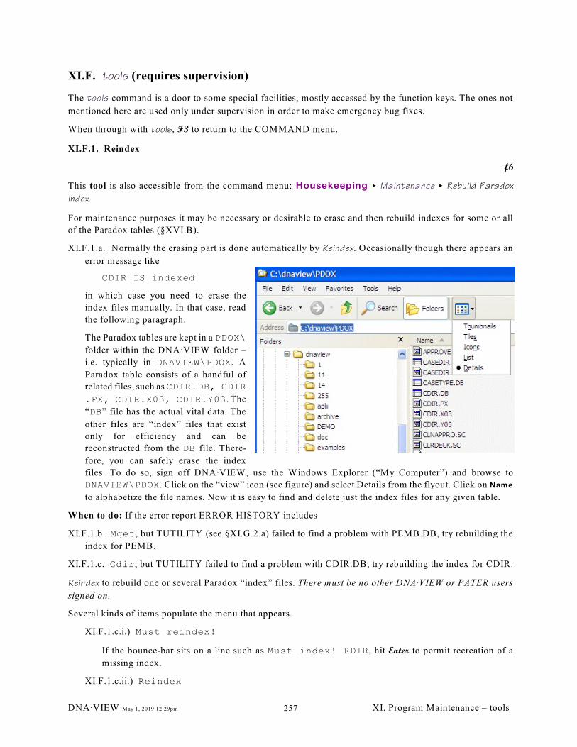
XI.F. tools (requires supervision)
The tools command is a door to some special facilities, mostly accessed by the function keys. The ones not
mentioned here are used only under supervision in order to make emergency bug fixes.
When through with tools, F3 to return to the COMMAND menu.
XI.F.1. Reindex
f6
This tool is also accessible from the command menu: Housekeeping < Maintenance < Rebuild Paradox
index.
For maintenance purposes it may be necessary or desirable to erase and then rebuild indexes for some or all
of the Paradox tables (§XVI.B).
XI.F.1.a. Normally the erasing part is done automatically by Reindex. Occasionally though there appears an
error message like
CDIR IS indexed
in which case you need to erase the
index files manually. In that case, read
the following paragraph.
The Paradox tables are kept in a PDOX\
folder within the DNA @VIEW folder –
i.e. typically in DNAVIEW\PDOX. A
Paradox table consists of a handful of
related files, such as CDIR.DB, CDIR
.PX, CDIR.X03, CDIR.Y03. The
“DB” file has the actual vital data. The
other files are “index” files that exist
only for efficiency and can be
reconstructed from the DB file. There-
fore, you can safely erase the index
files. To do so, sign off DNA@VIEW, use the Windows Explorer (“My Computer”) and browse to
DNAVIEW\PDOX. Click on the “view” icon (see figure) and select Details from the flyout. Click on Name
to alphabetize the file names. Now it is easy to find and delete just the index files for any given table.
When to do: If the error report ERROR HISTORY includes
XI.F.1.b. Mget, but TUTILITY (see §XI.G.2.a) failed to find a problem with PEMB.DB, try rebuilding the
index for PEMB.
XI.F.1.c. Cdir, but TUTILITY failed to find a problem with CDIR.DB, try rebuilding the index for CDIR.
Reindex to rebuild one or several Paradox “index” files. There must be no other DNAAVIEW or PATER users
signed on.
Several kinds of items populate the menu that appears.
XI.F.1.c.i.) Must reindex!
If the bounce-bar sits on a line such as Must index! RDIR, hit Enter to permit recreation of a
missing index.
XI.F.1.c.ii.) Reindex
DNA@VIEW May 1, 2019 12:29pm XI. Program Maintenance – tools257
Additionally, any index can be rebuilt by selecting a line such as Reindex CDIR.
Note: Needless rebuilding is harmless, except that it make take some minutes and must be allowed to
complete once initiated. (But if e.g. a power failure crashes the computer during rebuilding, there is
no disaster – just rebuild later.)
XI.F.1.c.iii.) Change Paradox library from: pdox\
This option provides a way to introduce or change the drive letter for the folder containing Paradox
tables. Normally thought the best choice is pdox\, without a drive letter and without the preceding
parts of the path.
XI.F.1.c.iv.) Change sort order from: ASCII
Don’t change the sort order unless you understand Paradox. Changing the sort order necessitates
rebuilding all indices.
XI.F.2. Push_Me
Select useful tools f1
Press f1, which is labeled Push_Me to obtain the set of user-semi-friendly and interesting tools which are
described below:
XI.F.3. Repair
Sometimes files that sit in one place on the disk for too long start to rot. Occasional use of FileCompress
(§X.K.6) will probably prevent this happening. However, if it does happen you will get an error with the error
message FILE DATA ERROR, indicating that some of the data in a file is corrupt.
The cure in that case is to use Repair, which will wipe out the corrupted portions of the file. The corrupt data
is irretrievably lost, but usually that’s not serious, and removing it at least enables DNA@VIEW to operate
without further trouble.
To invoke Repair, go to tools and type
Repair nn Enter
where nn is a number that designates the file to repair. You will need to contact DNA@VIEW support, with the
fax error message, to determine the right value for nn.
In cases of extreme damage, DNA@VIEW may abort during Repair — you may be dumped out of
DNA@VIEW, or the computer may even freeze. However, restart DNA@VIEW and restart Repair, and it will
delete the last bad spot and continue.
DNA@VIEW May 1, 2019 12:29pm XI. Program Maintenance – tools258
XI.G. Repair Paradox problems
The DnaView desktop folder has an icon called Repair that runs any of several operations that can be helpful
to resolve corruption problems that occasionally occur (e.g. by unceremonious shutdown of DNA@VIEW or
PATER such as by a power failure) with the Paradox tables that DNA@VIEW and PATER use for some kinds
of data.
There are certain files that occasionally become corrupt and thereby prevent proper operation of DNA@VIEW,
but which can easily be repaired. Repair is part of the solution.
XI.G.1. Reasons for trying Repair include
» the strange error message from DNA@VIEW Internal error no 226.
» Data posted from Paternity Case to PATER sometimes fails to show up.
» Data that was there yesterday seems to be missing today.
» The program begins an operation and never completes (but usually can be interrupted with Ctrl-
break).
» advice from the program author
XI.G.1.a. Don’t try Repair while there are any DNA@VIEW or PATER users.
XI.G.2. Repair operation.
Double-click on the Repair icon. Options include:
Q. Quit – exit from the Repair utility
F. Fix – Remove temporary Paradox locking files, which Paradox should have deleted but didn’t. It
can never hurt to do this provided there are no DNA@VIEW or PATER users on the system.
P. erase Pemb – Erase a certain expendable DNA @VIEW table, which will then automatically be
reconstructed when DNA@VIEW next starts.
R. erase Rdir – similar
D. erase DNAAPPRO – similar, except that this table is not re-constructible. The data, which is historical
case data useful for eventual study of mutation rates, will be lost.
The DNAAPPRO file is a communication file between DNA@VIEW and PATER. If data fails to reach
PATER from DNA·VIEW as it should, it may be because of corruption in DNAAPPRO. If so,
resetting it with this option is appropriate.
The drawbacks to erasing DNAAPPRO are:
» Any paternity cases that have been computed in DNA@VIEW but not yet retrieved in PATER
must be computed again (in Paternity Case).
» All old cases would need to be re-computed if it is desired to use the Mutation History
(§VIII.K) command to analyze them for mutations.
Possibly a corruption problem with DNAAPPRO can be repaired with TUTILITY (§XI.G.2.a).
P. Paradox – Offer to open the Paradox user interface, starting in the DNAVIEW Paradox directory, in case
of special maintenance work. (Note: Usually necessary to “Fix” first.) This options requires
that you have a Paradox user interface. It is not provided as part of the DNA@VIEW package.
T. Tutility – verify the integrity of a Paradox table, and offer to try to rebuild it.
DNA@VIEW May 1, 2019 12:29pm XI. Program Maintenance – tools259
XI.G.2.a. Tutility options
F. Fix – same as above. Also include in the Tutility menu because it is a likely prerequisite to the other
operations:
Verify any particular table, by typing in the table letter as indicated:
Rdir, Pdir, pEmb, Cdir, cAsedir, Namedir, Dnaappro, Strdata.
The result of “verify” will be one of three possibilities:
XI.G.2.a.i.) Table does not exist. This may mean the table is not essential, or may mean that it has been
erased or was never created. Starting DNA@VIEW will create any essential missing tables.
XI.G.2.a.ii.) Table verifies ok. Example:
Table Rdir verifies ok, but it is still possible it has a badindex.
Rebuild it anyway?
As the prompt implies, the verify doesn't verify everything so if you are suspicious of the table, rebuild
it.
XI.G.2.a.iii.) Table doesn't verify ok. Rebuild recommended.
The disadvantage of rebuilding is that rebuilding doesn't work as well as it should. It probably
reconstructs the table ok (depends how bad the damage is), but it is likely not to reconstruct correctly
some associated files called “index” files.
» Therefore, note any tables that you rebuild and subsequently, Reindex (§XI.F.1) them in
DNA@VIEW.
Note that there are two tables that DNA @VIEW can re-construct completely, namely RDIR and PEMB (see
above). Therefore there is no particular point in rebuilding these. You may as well erase them completely and
let DNA@VIEW rebuild them.
DNA@VIEW May 1, 2019 12:29pm XI. Program Maintenance – tools260
XII. EVALUATION OF EVIDENCE
XII.A. Concepts
We are concerned with a question of evaluation of scientific evidence.
XII.A.1. Scientific Decision Making; a Primer
The following point of view is about as general as you can get:
XII.A.1.a. There is a hypothesis to confirm or deny.
Example 1:
1H = this man is the father – as opposed to
0H = this man is not the father.
In practice though in order to be able to calculate we usually need a more explicit alternative hypothesis,
2such as H = a random (unrelated) Caucasian man is the father
Example 2:
1H = this stain comes from the suspect
2H = this stain comes from a brother of the suspect
Example 3:
1H = the children are full siblings
2H = the children are half siblings
XII.A.1.b. There is scientific evidence
There is some scientific evidence, E. For our purposes, E always consists of the various DNA types from
some blood and/or stain specimens. To say that evidence is scientific really just means that its significance
is objectively quantifiable. The quantity is that mentioned below in §XII.A.1.c.
There will always be other evidence also, known as the anecdotal evidence, about which the laboratory
presumes to know nothing.
XII.A.1.c. There are probabilities
It is possible to calculate the conditional probabilities
DNA@VIEW May 1, 2019 12:29pm XII. Evaluation of Evidence261
1X = Pr(E | H ) and
0Y = Pr(E | H ).
Pr(E) means the probability (fraction of all occasions) — some number between 0 and 1 inclusive — that
E occurs. Pr(E | H) means the “conditional probability of E given H.” I.e. it is the fraction of the time that
E occurs among those times that H occurs. These
Discussion::
XII.A.1.c.i.) This requirement explains what it means that the scenarios must be explicit. Thus “this man
is not the father” is usually insufficiently explicit, because to calculate a probability may require
making further assumptions about how likely it is that the father and “this man” are related, or about
the race of the father. Nonetheless, we won’t belabor this point, but will tacitly assume in the examples
0 1that H is true if H is false.
0XII.A.1.c.ii.) Normally H is formulated in such a way that Y is not 0. It may happen that X=0, which
0renders the alternative H certain.
XII.A.1.d. Prior Probability
To understand what the scientist should calculate and report, it is necessary to consider the decision
problem from the judge’s point of view. Imagine that the judge considers the anecdotal evidence first, and
1intuitively or consciously ascribes some “prior probability” p=Pr(H ). I.e., in a case of example 1 above,
the judge might think, “I don’t believe this woman very much. If I heard this story 1,000,000 times, the
man would probably be the father only about 100,000 times,” so the judge is thinking p=0.1.
XII.A.1.e. Using X and Y
But now we explain to the judge the evidence E and the values of X and Y. Suppose X=0.25 and
Y=0.00001. That means that of the 100,000 hypothetical cases in which the man is the father, E would be
observed 100,000A0.25 = 25,000 times, whereas of the 900,000 times that the man is not the father, E
occurs only 900,000A0.00001 = 90 times.
XII.A.1.f. Posterior Probability
The judge now reconsiders. “If I heard this case 1,000,000 times, I would see the evidence E a total of
25,090 times. Since we have evidence E, this case must be one of those 25,090. Those cases represent
25,000 cases where the man is the father, and only 90 cases where he is a coincidental victim. So it must
be 25,000:90 or 99.64% (=25000/25090) that this man is the father.”
XII.A.1.g. Bayes Theorem
It is important that the last paragraph be clearly understood. The reasoning that it embodies, albeit in
concrete rather than symbolic form, is commonly known as Bayes’ Theorem. Does it seem fishy to you
that we can forget about the original 1,000,000 cases and imagine ourselves swimming randomly among
the 25,090 “relevant” cases? Perhaps you should be suspicious at first; it certainly shows that you are
ipaying attention, and in fact there is something clever about the point of view. Pr(H |E) (i=0, 1) is what
ithe judge needs to evaluate. Pr(E|H ) is what the scientist can compute, and is quite a different thing. How
do you obtain one from the other? You should study the reasoning until it makes sense.
You may have heard that there exist “non-Bayesian” mathematicians. If you continue to feel uncomfort-
able with the logic, perhaps you are tempted to categorize yourself as a non-Bayesian and give up. I cannot
condone this route. To the best of my understanding, the non-Bayesians’ quarrel is not with the logic, but
with the philosophy of assigning a prior probability. Since as a practical matter the judge only needs some
absurdly conservative lower bound for p, personally I don’t think there is any sensible ground to take the
non-Bayesian tack here. However even a doctrinaire extreme non-Bayesian will understand the Bayesian
logic and dispute only its applicability.
DNA@VIEW May 1, 2019 12:29pm XII. Evaluation of Evidence262
Note that the probabilities in the numerator and
denominator of a likelihood ratio need not sum to
unity nor to any other particular value. Hence a
likelihood ratio is quite different from an “odds
ratio,” which, at least as used here, is an
expression of the form
Pr(E | H) / Pr(~E | H)
where the numerator and denominator represent
probabilities of complementary events based on
the same hypothesis, and which therefore do sum
to unity.
Put otherwise, suppose you have a likelihood
ratio of 9. It can of course be written in the form
0.9 / 0.1, numerator and denominator adding to 1,
but it doesn’t follow that there is any meaning to
0.9 or 0.1 as a probabilities. On the other hand, if
the odds ratio for some event (e.g. paternity) is 9,
then the probabilities 0.9 and 0.1 represent the
probabilities of paternity and non-paternity
respectively.
By contrast, multiplying an odds ratio (e.g. prior
odds) by a likelihood ratio does result in an odds
ratio. (e.g. posterior odds).
Likelihood ratio vs. Odds ratio
XII.A.1.h. Paternity index
Before leaving this section, we need to summarize the judge’s reasoning in symbolic form. The simplest
form will be obtained by using this tip, which will be a revelation to your statistician colleagues: formulate
in terms of “odds” or “odds ratio” like the horse players do, rather than probabilities like a mathematician.
I.e. the judge’s initial judgement of probability p corresponds to odds of p:1!p. (The : means divided by.
So you can say the odds are “p to 1!p” or you can say “p/(1!p) to 1” or you can just say “an odds ratio
of p/(1!p),” all of which mean that it happens p times for every 1!p times it doesn’t happen.) On hearing
the scientific data, the judge’s estimate of the odds change from p:(1!p) to pX:(1!p)Y. The judge’s odds
ratio is multiplied by X/Y.
XII.A.2. The Likelihood Ratio
Therefore, the scientific evidence is completely
summarized by the ratio X/Y. A ratio of this form is
called a likelihood ratio. Precisely defined, a likeli-
hood ratio is defined to be an expression of the form:
1 0Pr(E | H ) / Pr(E | H ),
that is, the ratio of two probabilities representing the
chance of the same event under mutually exclusive
hypotheses.
So each of X and Y by itself is unimportant. Only
the ratio matters. And the scientist need not be
concerned with, nor make any assumptions about,
the prior odds or the anecdotal evidence.
In a paternity case, we call this likelihood ratio PI
(Paternity Index); in a forensic case, matching LR.
Formulated in terms of probabilities rather than odds
ratios, the probability of paternity W is given by the
expression:
W = pX / (pX + (1!p)Y), (*)
which can also be written , which
exemplifies the relationship probability = oddsratio
/ (oddsratio+1) to convert between probability and
odds ratio formulations.
Here is a convenient fact about the odds ratio formulation. Suppose that after we finish explaining E to the
judge and provide him or her with the corresponding likelihood ratio, some other scientist comes to the witness
stand to discuss the ballistic evidence. The judge has only to multiply to account for each new piece of
evidence:
odds ratio = (prior odds ratio)A(DNA likelihood ratio)A(ballistic likelihood ratio)A...
DNA@VIEW May 1, 2019 12:29pm XII. Evaluation of Evidence263
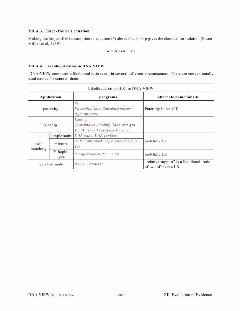
XII.A.3. Essen-Möller’s equation
Making the (unjustified) assumption in equation (*) above that p=1!p gives the classical formulation (Essen-
Möller et al, 1939):
W = X / (X + Y).
XII.A.4. Likelihood ratios in DNA@VIEW
DNA@VIEW computes a likelihood ratio result in several different circumstances. There are conventionally
used names for some of them.
Likelihood ratios (LR) in DNA@VIEW
Application programs alternate name for LR
paternity
PI
Paternity Index (PI)Paternity Case Calculate patern-
ity/maternity
kinship
Kinship
[Automatic Kinship] Case immigra-
tion/kinship, Prototype Kinship
stain
matching
simple stain DNA odds, DNA profiles
matching LRmixture
Automatic mixture, Mixture Calcula-
tor
Y-haplo-
typeY-haplotype matching LR matching LR
racial estimate Racial Estimate“relative support” is a likelihood; ratio
of two of them a LR
DNA@VIEW May 1, 2019 12:29pm XII. Evaluation of Evidence264
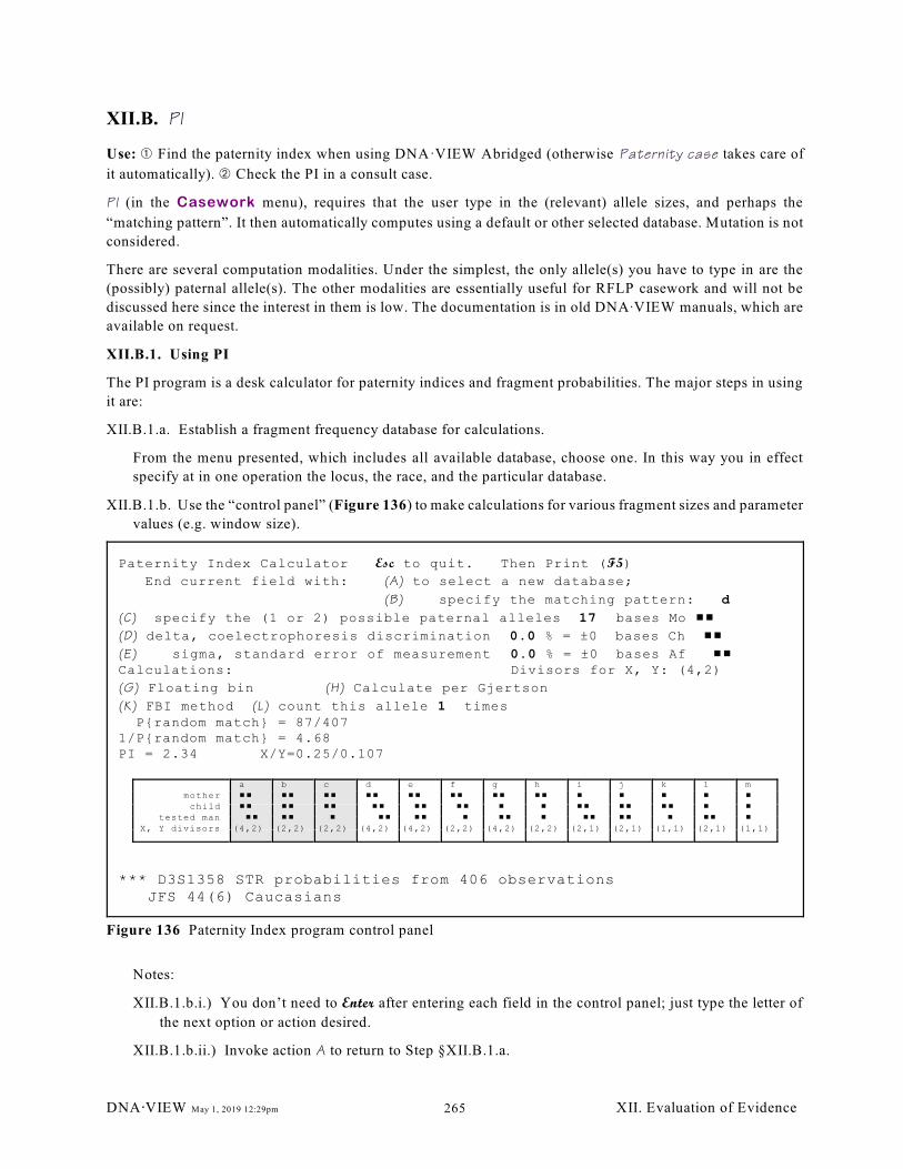
Paternity Index Calculator Esc to quit. Then Print (F5)
End current field with: (A) to select a new database;
(B) specify the matching pattern: d
(C) specify the (1 or 2) possible paternal alleles 17 bases Mo ##
(D) delta, coelectrophoresis discrimination 0.0 % = ±0 bases Ch ##
(E) sigma, standard error of measurement 0.0 % = ±0 bases Af ##Calculations: Divisors for X, Y: (4,2)
(G) Floating bin (H) Calculate per Gjertson
(K) FBI method (L) count this allele 1 times P{random match} = 87/4071/P{random match} = 4.68PI = 2.34 X/Y=0.25/0.107
motherchild
tested manX, Y divisors
a ## ## ##(4,2)
b ## ## ##(2,2)
c ## ## #(2,2)
d ## ## ##(4,2)
e ## ## ##(4,2)
f ## ## #(2,2)
g ## # ##(4,2)
h ## # #(2,2)
i # ## ##(2,1)
j # ## ##(2,1)
k # ## #(1,1)
l # # ##(2,1)
m # # #(1,1)
*** D3S1358 STR probabilities from 406 observations JFS 44(6) Caucasians
Figure 136 Paternity Index program control panel
XII.B. PI
Use: â Find the paternity index when using DNA·VIEW Abridged (otherwise Paternity case takes care of
it automatically). ã Check the PI in a consult case.
PI (in the Casework menu), requires that the user type in the (relevant) allele sizes, and perhaps the
“matching pattern”. It then automatically computes using a default or other selected database. Mutation is not
considered.
There are several computation modalities. Under the simplest, the only allele(s) you have to type in are the
(possibly) paternal allele(s). The other modalities are essentially useful for RFLP casework and will not be
discussed here since the interest in them is low. The documentation is in old DNAAVIEW manuals, which are
available on request.
XII.B.1. Using PI
The PI program is a desk calculator for paternity indices and fragment probabilities. The major steps in using
it are:
XII.B.1.a. Establish a fragment frequency database for calculations.
From the menu presented, which includes all available database, choose one. In this way you in effect
specify at in one operation the locus, the race, and the particular database.
XII.B.1.b. Use the “control panel” (Figure 136) to make calculations for various fragment sizes and parameter
values (e.g. window size).
Notes:
XII.B.1.b.i.) You don’t need to Enter after entering each field in the control panel; just type the letter of
the next option or action desired.
XII.B.1.b.ii.) Invoke action A to return to Step §XII.B.1.a.
DNA@VIEW May 1, 2019 12:29pm XII. Evaluation of Evidence265
XII.B.1.b.iii.) Option C allows 1 or 2 sizes. You might then be forced to select a consistent pattern at
Option B.
XII.B.1.b.iv.) Parameter changes are temporary. Use window size (from locus maintenance, §IX.B.2) to
change them permanently.
XII.B.2. PI program examples
PI for paternal allele 17, using default parameters and database:
At prompt C, type 17g. (17 is the allele, g requests the computation.)
PI for same problem, but temporarily overriding the parameter to “count observed allele in database” (per
§V.C.4.a):
At prompt C, type l0g (letter l, number 0)
PI for the ambiguous paternal allele when Mother=Child=17,18; man is 18, 19:
At prompt C, type 17 18bag. (17 18 are the alleles, b refers to the matching pattern prompt B, a selects
the pattern, g requests the computation.)
PI for the same problem, different database:
At prompt C, type a for the database menu, D3SABIBlack enter to select the D3S1358, ABI, Black
database, g to compute.
XII.B.3. PI control panel discussion
XII.B.3.a. Calculation options
Three methods are offered. to calculate versions of the allele probability.
XII.B.3.a.i.) G Window/floating bin method
Method G is essentially the floating bin approach. A bin size of 0 gives a discrete allele system which
is usual for PCR data, although occasionally you may use e.g. a 1% bin to get the effect of lumping
TH01 9.3 and 10 together. It takes into account the specified band pattern among the three tested
individuals to compute a PI.
XII.B.3.a.ii.) H Gjertson method – RFLP only
XII.B.3.a.iii.) K FBI method – RFLP only (“fixed bin”)
XII.B.3.b. Using the control panel
A special method of operation applies to the control panel — instead of ending an entry with Space or
Enter as is typical, end by typing the letter (A!H) of the next desired action/choice. The meanings of the
various letters are:
(A) action: go back to select another database / locus / race. (The currently active database is listed at the
bottom of the screen.)
(B) choice: select a matching pattern from those displayed in the middle bottom of the screen. Each
pattern represents a possible band pattern for a trio. For example, pattern f (see Figure 136) should
be selected when a heterozygous child matches one allele with its heterozygous mother and the other
with its homozygous father.
DNA@VIEW May 1, 2019 12:29pm XII. Evaluation of Evidence266
If there are two lengths at (C), then the possible choices here will be a, b, c, corresponding to patterns
with mother and child matching two alleles. If there is only one length at (C), then the possible choices
will be d!m, which are explained by schematics corresponding to the various possible matching pat-
terns for the trio.
The pair of numbers listed as “divisors” are shown only to explain the role that the matching diagram
plays in the PI calculation. The first divisor is 4, 2, or 1 according as X is ¼, ½, or 1. The second
divisor is divided into the allele probability to obtain Y.
The answer to (B) is just one letter. Where you go next is either where you had asked to go before
detouring to (B), or, otherwise, (C).
(C) parameter: the size(s) (allele number of base pairs) of the one or two possible paternal alleles. If you
give an answer to (C) that isn’t consistent with the current choice at (B), then you’ll be required to
make a consistent specification for (B) before proceeding.
How does the program know if you mean allele number or base pair size? Any number less than 100
will be interpreted as a repeat number; greater, a length in base pairs. To specify an allele$100, prefix
it with #, such as #123 means allele #123.
(D) parameter: delta (ä), the co-electrophoresis resolution threshold (half the size of the “matching
window”), as a % of molecular weight. For discrete allele systems such as STR’s, it is usually
appropriate to use ä=0.
(L) parameter: t, the number of extra times to include this allele in the database. The reference value is set
using the option Count observed allele in database how many times? (V.C.4.a) in Case, options (also
accessible as options from "Case" under Options).
The remark about Temporary values above applies to this parameter also.
(G) action: Calculate PI using all of the above information.
Just below the control panel, the allele probability, and 1/allele probability are displayed in red letters.
Below that the PI is shown in red, and any previous PI’s in are scrolled down so that the results of the
last few calculations persist on the screen.
The PI is labeled briefly as to the method of calculation (floating bin for computation G). A
complete synopsis of the result and calculation parameters is appended to the log, which may later be
printed using Print.
When you request computation G and the currently selected band pattern (field B) isn’t consistent with
the specified number of paternal alleles, you are obliged to select a new pattern before the calculation
proceeds. See (B) above.
Esc action: exit from PI.
DNA@VIEW May 1, 2019 12:29pm XII. Evaluation of Evidence267
XII.C. Paternity Index Discussion
The paternity index, PI, is a summary of the evidentiary value of the data. It is not an ad hoc statistic (as most
statistical measures are) whose interpretation depends on tables and relative comparisons. Rather, formulae
for PI are derived by an inevitable chain of mathematical reasoning starting from assumptions about the
experimental process — i.e. starting from a (mathematical) model of the experimental process. As such, PI has
an explicit and real meaning, which may be expressed by such sentences as:
(a) All other things being equal, this man is PI times as likely to be the father as not;
(b) Assuming a prior probability p of paternity, in light of the genetic evidence the probability of paternity
is
W = pAPI / (pAPI + 1!p);
(c) In light of the genetic evidence the prior odds should be multiplied by PI.
(c) and (b) are the same statement in terms of odds or in terms of probabilities. (a) is an informal statement of
(c) for the specific case of prior odds of 1:1 (“all other things being equal”). In any case, think of PI as being
an inference from the data.
DNA@VIEW May 1, 2019 12:29pm XII. Evaluation of Evidence268
XII.D. Explaining the result
Classically people considered three statistics concerning paternity:
(1) A=exclusion probability
or its close cousin RMNE=1!A. The more quickly this historical but misguided statistic is forgotten, the
better. That is particularly true in extended family analysis, where it often is the case that no combination
of alleles at all can lead to exclusion. Nonetheless, the case may be eminently decidable.
(2) LR=L=likelihood ratio
This is the fundamental statistic, although in the case of paternity it is usually called the PI or “paternity
index.”
(3) W=probability
In the paternity case, W=probability of paternity. The present context may require different words of
course.
Of the latter two statistics above, W is the apparently easier to explain and understand, especially if one is not
inclined to concern oneself about the sticky question of “prior probabilities.” Assuming for example that the
issue is between paternity and unrelatedness, W answers the question
“What is the probability of paternity, in light of (=assuming) the genetic evidence (and also assuming a
prior probability of 50%, or of p).”
The likelihood ratio has the merit of summarizing the scientific evidence without being polluted by non-
scientific assumptions (prior probabilities), but it has the disadvantage of being unfamiliar and difficult to
explain in English. As a starting point, it helps to realize that
the likelihoods (in the likelihood ratio) are probabilities of the genetic evidence assuming paternity or
assuming non-paternity.
Thus, what is an assumption for W is a conclusion for the LR, and vice-versa. A likelihood ratio of 32 does
not mean paternity is 32 times more likely than non-paternity. It means the evidence is 32 times more likely
assuming paternity than assuming non-paternity.
To see the difference, consider this imaginary situation. A man is accused of paternity in Wisconsin and the
LR turns out to be 32. Probably he is the father, I admit. But suppose that in the future we genetically screen
the whole earth population and find a five-year-old child in Tibet who has the same DNA results in the tested
loci. The LR is therefore 32 for him (or her) as well. But he or she is probably not the father. So the LR alone
cannot properly be interpreted as implying paternity.
The question remains, how to explain a LR to a lay person. I suggest using the wording “characteristic of.”
Example phrasings for two situations are given below.
XII.D.1.a. Paternity question; moderate evidence
For the example case of the preceding few sections comparing paternity versus nonpaternity and with
likelihood ratio computed in §IX.E.11, the result can be stated as follows:
LR explanation:
“The observed genetic results are 32 times more characteristic of paternity than of non-paternity (i.e.
unrelatedness). That is, they are moderately strong evidence favoring the former vis-a-vis the latter
hypothesis.”.
W explanation:
DNA@VIEW May 1, 2019 12:29pm XII. Evaluation of Evidence269
“If, prior to genetic testing, the two hypotheses were assumed to be equally likely (50% prior
probability of paternity), then taking the tests into account increases the probability of paternity
to 97%. If some other prior probability assumption were made, then the result would be somewhat
different.”
XII.D.1.b. Missing body; powerful evidence
Scenario: A body in the woods is tested and compared with a family that has reported a missing child.
The combined likelihood ratio is 1,234,000.
LR explanation:
“The observed genetic results are about a million times better explained by assuming that the body
is indeed the missing child, than by imagining they are unrelated. If these are the possibilities, the
evidence that the body is the child is overwhelming.”
W explanation:
“If, prior to genetic testing, the two possibilities were assumed to be equally likely (50% prior
probability), then taking the tests into account increases the probability to 99.9999% — virtual
certainty — that the body is the missing child. If some other prior probability assumption were
made, then the numerical result would be slightly different. However it is hard to imagine a
scenario that would change the result materially.”
DNA@VIEW May 1, 2019 12:29pm XII. Evaluation of Evidence270
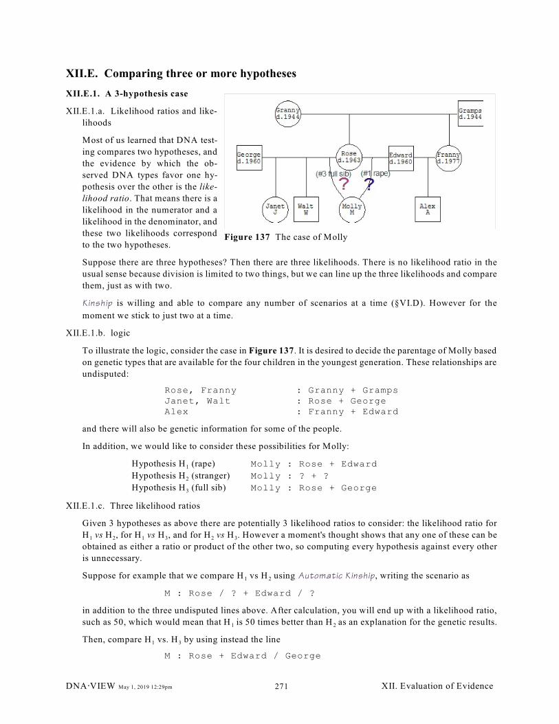
Figure 137 The case of Molly
XII.E. Comparing three or more hypotheses
XII.E.1. A 3-hypothesis case
XII.E.1.a. Likelihood ratios and like-
lihoods
Most of us learned that DNA test-
ing compares two hypotheses, and
the evidence by which the ob-
served DNA types favor one hy-
pothesis over the other is the like-
lihood ratio. That means there is a
likelihood in the numerator and a
likelihood in the denominator, and
these two likelihoods correspond
to the two hypotheses.
Suppose there are three hypotheses? Then there are three likelihoods. There is no likelihood ratio in the
usual sense because division is limited to two things, but we can line up the three likelihoods and compare
them, just as with two.
Kinship is willing and able to compare any number of scenarios at a time (§VI.D). However for the
moment we stick to just two at a time.
XII.E.1.b. logic
To illustrate the logic, consider the case in Figure 137. It is desired to decide the parentage of Molly based
on genetic types that are available for the four children in the youngest generation. These relationships are
undisputed:
Rose, Franny : Granny + GrampsJanet, Walt : Rose + GeorgeAlex : Franny + Edward
and there will also be genetic information for some of the people.
In addition, we would like to consider these possibilities for Molly:
1Hypothesis H (rape) Molly : Rose + Edward
2Hypothesis H (stranger) Molly : ? + ?
3Hypothesis H (full sib) Molly : Rose + George
XII.E.1.c. Three likelihood ratios
Given 3 hypotheses as above there are potentially 3 likelihood ratios to consider: the likelihood ratio for
1 2 1 3 2 3H vs H , for H vs H , and for H vs H . However a moment's thought shows that any one of these can be
obtained as either a ratio or product of the other two, so computing every hypothesis against every other
is unnecessary.
1 2Suppose for example that we compare H vs H using Automatic Kinship, writing the scenario as
M : Rose / ? + Edward / ?
in addition to the three undisputed lines above. After calculation, you will end up with a likelihood ratio,
1 2such as 50, which would mean that H is 50 times better than H as an explanation for the genetic results.
1 3Then, compare H vs. H by using instead the line
M : Rose + Edward / George
DNA@VIEW May 1, 2019 12:29pm XII. Evaluation of Evidence271
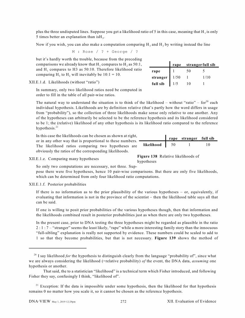
rape stranger full sib
rape 1 50 5
stranger 1/50 1 1/10
full sib 1/5 10 1
rape stranger full sib
likelihood 50 1 10
Figure 138 Relative likelihoods of
hypotheses
1plus the three undisputed lines. Suppose you get a likelihood ratio of 5 in this case, meaning that H is only
35 times better an explanation than isH .
3 2Now if you wish, you can also make a computation comparing H and H by writing instead the line
M : Rose / ? + George / ?
but it’s hardly worth the trouble, because from the preceding
1 2comparisons we already know that H compares to H as 50:1,
1and H compares to H3 as 50:10. Therefore likelihood ratio
3 2comparing H to H will inevitably be 10:1 = 10.
XII.E.1.d. Likelihoods (without “ratio”)
In summary, only two likelihood ratios need be computed in
order to fill in the table of all pair-wise ratios.
The natural way to understand the situation is to think of the likelihood – without “ratio” – for each20
individual hypothesis. Likelihoods are by definition relative (that’s partly how the word differs in usage
from “probability”), so the collection of three likelihoods make sense only relative to one another. Any
of the hypotheses can arbitrarily be selected to be the reference hypothesis and its likelihood considered
to be 1; the (relative) likelihood of any other hypothesis is its likelihood ratio compared to the reference
hypothesis.21
In this case the likelihoods can be chosen as shown at right,
or in any other way that is proportional to these numbers.
The likelihood ratios comparing two hypotheses are
obviously the ratios of the corresponding likelihoods.
XII.E.1.e. Comparing many hypotheses
So only two computations are necessary, not three. Sup-
pose there were five hypotheses, hence 10 pair-wise comparisons. But there are only five likelihoods,
which can be determined from only four likelihood ratio computations.
XII.E.1.f. Posterior probabilities
If there is no information as to the prior plausibility of the various hypotheses – or, equivalently, if
evaluating that information is not in the province of the scientist – then the likelihood table says all that
can be said.
If one is willing to posit prior probabilities of the various hypotheses though, then that information and
the likelihoods combined result in posterior probabilities just as when there are only two hypotheses.
In the present case, prior to DNA testing the three hypotheses might be regarded as plausible in the ratio
2 : 1 : 7 – “stranger” seems the least likely, “rape” while a more interesting family story than the innocuous
“full-sibling” explanation is really not supported by evidence. These numbers could be scaled to add to
1 so that they become probabilities, but that is not necessary. Figure 139 shows the method of
I say likelihood for the hypothesis to distinguish clearly from the language “probability of”, since what20
we are always considering the likelihood (=relative probability) of the event, the DNA data, assuming one
hypothesis or another.
That said, the to a statistician “likelihood” is a technical term which Fisher introduced, and following
Fisher they say, confusingly I think, “likelihood of”.
Exception: If the data is impossible under some hypothesis, then the likelihood for that hypothesis21
remains 0 no matter how you scale it, so it cannot be chosen as the reference hypothesis.
DNA@VIEW May 1, 2019 12:29pm XII. Evaluation of Evidence272
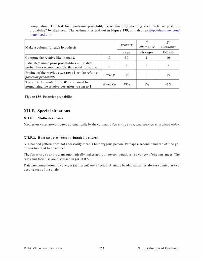
Make a column for each hypothesisprimary
1st
alternative
2nd
alternative
rape stranger full sib
Compute the relative likelihoods L L 50 1 10
Estimate/assume prior probabilities p. Relative
probabilities is good enough; they need not add to 1.p 2 1 7
Product of the previous two rows is w, the relative
posterior probabilityw=L×p 100 1 70
The posterior probability, W, is obtained by
normalizing the relative posteriors to sum to 1W=w/3w 58% 1% 41%
Figure 139 Posterior probability
computation. The last line, posterior probability is obtained by dividing each “relative posterior
probability” by their sum. The arithmetic is laid out in Figure 139, and also see http://dna-view.com/
manyhyp.htm).
XII.F. Special situations
XII.F.1. Motherless cases
Motherless cases are computed automatically by the command Paternity case , calculate paternity/maternity.
XII.F.2. Homozygotes versus 1-banded patterns
A 1-banded pattern does not necessarily mean a homozygous person. Perhaps a second band ran off the gel
or was too faint to be noticed.
The Paternity case program automatically makes appropriate computations in a variety of circumstances. The
rules and formulas are discussed in §XIII.B.5.
Database compilation however, is (at present) not affected. A single banded pattern is always counted as two
occurrences of the allele.
DNA@VIEW May 1, 2019 12:29pm XII. Evaluation of Evidence273

DNA@VIEW May 1, 2019 12:29pm XII. Evaluation of Evidence274
XIII. ALGORITHMS
This chapter discusses in detail the way that DNA@VIEW performs some of its computations.
XIII.A. Probability computations
XIII.A.1. Match window probability
The purpose of this section is to explicitly document the details of the window computation.
Assume that a allele is given and a particular data base has been selected. There are a number of parameters
and stages to the computation.
XIII.A.1.a. Band size in bases
Internally all alleles, even STR alleles, are expressed as some number of base pairs, possibly fractional.
(However, whether the fraction is displayed depends on the setting of Options §IX.F.28.d).
The STR size is related to the allele number using the PCR parameters (§XIII.B.1) that have been defined
by the user for that locus.
Let s denote the size of the allele in question.
XIII.A.1.b. Determine ä (delta)
The value of ä is the “Match window” number that the user sets as discussed in §VII.B.2 such as 0 or 1%.
XIII.A.1.c. The match window
The basic meaning of ä is that two measurements more than ä apart are assumed to represent different
sources.
ä determines the amount to be added and subtracted from s to determine the match window. To be precise,
the match window is the interval from
s!sä to s+sä inclusive.
For example, suppose ä=1% for TH01, and consider the match window around the TH01 allele 9.3.
Suppose that the “size of allele #0" (§IX.B.3.a) for TH01 is defined as 134bp. Then
s = 134+(9x4)+3 = 173bp.
So sä = 1.7 bp.
Consequently the interval [s!sä, s+sä] includes 9.2, 9.3, and 10, so
DNA@VIEW May 1, 2019 12:29pm XIII. Algorithms275
» alleles reported as 9.3 and as 10 would be regarded as matching
» database entries for these sizes would be added for purposes of counting the 9.3 probability.
XIII.A.1.d. The floating bin probability
Suppose the number of database alleles that are within the window as defined above is k, and that there
are N alleles in the database altogether. Then define
0f (s) = k / N.
XIII.A.1.e. Adjustment
It remains to apply the effect of the options governing probability calculation. Let
m= Minimum # of matching alleles to assume for frequency calculations (V.C.4.b),
t= Count observed allele in database how many times (V.C.4.a),
XIII.A.1.e.i.) Adjust allele count
Using m=minimum #, t=count observed alleles times, N=alleles in database, we calculate the effective
number of matching alleles k as
k = max(m, t+f(s)N).
Note that for discrete-allele systems such as STR that f(s)N simply means the allele count that appears
in the database.
One further exceptional refinement: If Calculate crime allele frequencies simultaneously? is y, the
command DNA odds (only) “tosses in” two alleles when the type is homozygotes (regardless of
whether the profile is typed in with one copy or two). Hence in this case k = max(m, 2t+f(s)N).c
To represent counting the allele as part of the database, and adjustment is also needed to the size of
the database. Therefore we calculate
N’ = max(m, at+N)
where ordinarily a=1, but if both
Calculate crime allele frequencies simultaneously? (V.C.4.e) is y and
the command is a crime calculation (Automatic mixture, Mixture ("LR") calculator, DNA odds,
Y-haplotype matching LR or DNA exclusion),
then a means the number of alleles that are reported at the locus, meaning the number of alleles that
are typed in. (However, again in the case of DNA odds only, always a=2).
XIII.A.1.e.ii.) Probability
The reported probability is
f = k / N’.
XIII.A.1.e.iii.) Examples illustrating “adjustments”
Suppose that 1=m= Minimum # of matching alleles to assume for frequency calculations
1=t= Count observed allele in database how many times,
and that alleles 14 15 16 occur in the database with counts 1/200, 5/200, 10/200.
DNA@VIEW May 1, 2019 12:29pm XIII. Algorithms276

If the alleles are 14 15, then for purposes of Paternity Case (including immigration/kinship) or PI, or
even for crime cases if Calculate crime allele frequencies simultaneously? is n (which is recom-
mended), the probabilities are 2/201 and 6/201.
If the DNA odds genotype is 14 15 and Calculate crime allele frequencies simultaneously? is y, the
probabilities are 2/202 and 6/202.
If the DNA odds genotype is 16 and Calculate crime allele frequencies simultaneously? is y, the allele
probability is 12/202.
DNA@VIEW May 1, 2019 12:29pm XIII. Algorithms277
XIII.B. Computation of Paternity Index
XIII.B.1. Basic approach (window style)
Assuming that match-binning (i.e. windows, floating bins, not the Gjertson method) is used for paternity
calculation, the approach and formulas are basically as described in the American Association of Blood Banks
“Parentage Testing Accreditations Requirements Manual.”
By definition the paternity index L is L=X/Y, where DNA·VIEW takes
X = Pr(child as observed | woman & tested man are the parents), and
Y = Pr(child as observed | woman & random man are the parents).
Note that these definitions mean that X will be ¼ in the most typical situation where everyone is heterozygous,
and will also normally take on the value ½ or 1 depending on the pattern of apparent matching among the trio.
The Y value is q/2 in the common case where there is a clear-cut paternal allele and it has probability q. The
factor ½ corresponds to the fact that the woman is only 50% to transmit the maternal allele.
To those who object that she must be not 50% but 100% to pass the maternal allele because she is certainly
the mother, the answer is that this objection comes from ignoring the definition of Y and trying to answer some
other question instead. Another way to answer the objection is to point out that the same factor of ½ will occur
in X. The two ½ factors ultimately cancel one another when L is computed.
XIII.B.2. Matching patterns
The mother-child-father types follow one of the 13 or patterns shown in the PI panel, Figure 136 in
§XII.B.1.b. At the bottom of each pattern are a pair of numbers labeled “X, Y divisors,”such as 4,2 for the
pattern Mother=PR, Child=QR, Man=QS. The “4” means that X=¼. The “2” means the Y=q/2 where q is the
probability (in the sense of §XIII.A.1) of the paternal allele Q.
XIII.B.3. Paternal alleles
When it is not clear which allele is the paternal one, q is a weighted average of the probabilities of the possible
paternal alleles.
Thus when Mother=Child=QR, either allele might be paternal and either allele is equally likely to be paternal.
The appropriate weighting is ½, ½; i.e. q= ½Pr(Q) + ½Pr(R).
XIII.B.4. Motherless case
Formulas to compute the Paternity Index in a motherless case are described in Brenner (1993), and may also
be obtained from the Kinship (Chapter VI) program. For example, in the typical situation
Child P Q
Tested Man Q R
where P, Q, R are fragment sizes with respective probabilities p, q, r,
PI = 1/(4q).
Obviously X and Y can be chosen infinitely many ways so that PI=X/Y. DNA@VIEW reports X=(½)p/(p+q)
and Y=2qp/(p+q). The common normalizing factor 1/(p+q) represents the idea that mythical “Mother” Nature
contributes a P or Q for sure, but in the same ratio p:q as does Nature. On average X=1/4 about.
DNA@VIEW May 1, 2019 12:29pm XIII. Algorithms278
It may seem obvious to cancel p/(p+q) from both X and Y but this idea has no analogue when the man is
excluded. On the other hand, X=1/(2p) and Y=2pq is perfectly defensible but is inconvenient because it gives
such small numbers for X and for Y compared to a trio case.
XIII.B.5. Homozygosity vs. single-allele
If the (pheno-)type determined at some locus is 12, does it mean 12,12 or 12,null?
There several situations in which the assessment of paternity may vary depending on whether a one-allele
phenotype is assumed to represent a homozygous person, or whether the possibility is also considered that it
represents a person with two different alleles one of which is does not produce an experimental result –
normally because a primer binding site mutation (inherited, not a new mutation) causes failure of primer
hybridization.
In order to account for such a possibility, DNA·VIEW allows including a number of null alleles as part of any
database. I use the symbol o for this parameter. “Overlooked,” “unobserved,” “null,” “silent,” and “invisible”
all mean the same thing in the present discussion. The parameter o can also be specified on-the-fly during22
Paternity Case computation (§V.B.22).
The situations affected are
» PI computations by the Paternity case program when there is a single-allele phenotype,
» the DNA exclusion calculation for mixted stains.
Of the situations affected by the value (and non zero status) of o, the most important is the so-called “indirect
exclusion” — child and man are each single-allele, but different — but there are several other situations as
well.
XIII.B.5.a. Null alleles and databases
XIII.B.5.a.i.) Database compilation
Null alleles are not considered when DNAAVIEW compiles a database; every 1-allele type is treated as 2
alleles.
XIII.B.5.a.ii.) Putting nulls in the database
You need to edit a database manually (§VIII.C.12) in order to put nulls into it. You may or may not choose
to correspondingly remove some of the other alleles, depending on whether there are specific 1-allele types
that you believe include a null among the sample population.
XIII.B.5.b. Null alleles and Paternity Case calculate paternity/maternity calculation
Whenever any of the three people of a trio – mother, child, or alleged father – has a single-allele
phenotype, the calculation of paternity index is affected. Speaking generally the modification is that the
program considers two possibilities. If for example the person is 12, then the program considers both the
12,12 and the 12,null possible genotypes, and in accordance with Bayes’ theorem the relative probabilities
of each of these in the adults are in the proportion q to 2qo where q=Pr(12).2
In RFLP practice an allele or “band” may be overlooked because it ran off the end of the gel. As long22
as experimental conditions are held constant – so that the allele will always be overlooked – such an allele
is logically equivalent to any other null allele.
DNA@VIEW May 1, 2019 12:29pm XIII. Algorithms279
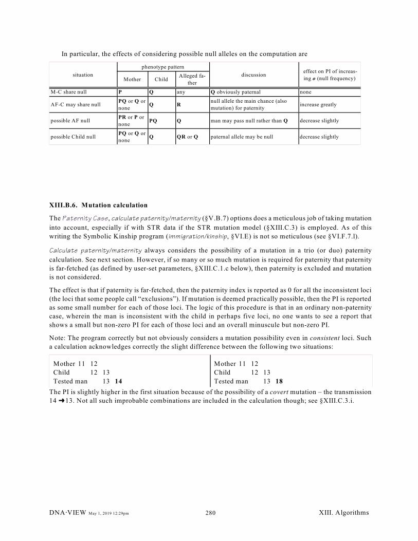
In particular, the effects of considering possible null alleles on the computation are
situation
phenotype pattern
discussion effect on PI of increas-
ing o (null frequency)Mother ChildAlleged fa-
ther
M-C share null P Q any Q obviously paternal none
AF-C may share nullPQ or Q or
noneQ R
null allele the main chance (also
mutation) for paternityincrease greatly
possible AF nullPR or P or
nonePQ Q man may pass null rather than Q decrease slightly
possible Child nullPQ or Q or
noneQ QR or Q paternal allele may be null decrease slightly
XIII.B.6. Mutation calculation
The Paternity Case , calculate paternity/maternity (§V.B.7) options does a meticulous job of taking mutation
into account, especially if with STR data if the STR mutation model (§XIII.C.3) is employed. As of this
writing the Symbolic Kinship program (immigration/kinship, §VI.E) is not so meticulous (see §VI.F.7.l).
Calculate paternity/maternity always considers the possibility of a mutation in a trio (or duo) paternity
calculation. See next section. However, if so many or so much mutation is required for paternity that paternity
is far-fetched (as defined by user-set parameters, §XIII.C.1.c below), then paternity is excluded and mutation
is not considered.
The effect is that if paternity is far-fetched, then the paternity index is reported as 0 for all the inconsistent loci
(the loci that some people call “exclusions”). If mutation is deemed practically possible, then the PI is reported
as some small number for each of those loci. The logic of this procedure is that in an ordinary non-paternity
case, wherein the man is inconsistent with the child in perhaps five loci, no one wants to see a report that
shows a small but non-zero PI for each of those loci and an overall minuscule but non-zero PI.
Note: The program correctly but not obviously considers a mutation possibility even in consistent loci. Such
a calculation acknowledges correctly the slight difference between the following two situations:
Mother 11 12
Child 12 13
Tested man 13 14
Mother 11 12
Child 12 13
Tested man 13 18
The PI is slightly higher in the first situation because of the possibility of a covert mutation – the transmission
14 º13. Not all such improbable combinations are included in the calculation though; see §XIII.C.3.i.
DNA@VIEW May 1, 2019 12:29pm XIII. Algorithms280
XIII.C. Mutation calculations
DNAAVIEW offers three models for dealing with possible mutations – Mendelian (no mutation, §XIII.C.2),
STR (modified step-wise, §XIII.C.3), Simple (old, pre-2005, AABB recommendation, §XIII.C.4).
XIII.C.1. Principles of mutation calculations
If at some locus in a paternity investigation, Mother=11,12, Child=12,13, Alleged father=14, then under
Mendelian genetics the PI=0. A more sophisticated and realistic model however acknowledges that this
pattern, though probably rare among true trios, is not impossible. That is, the right assessment is probably
some very small PI, 0<PI<<1.
To assess the entirety of the DNA data, the PI’s for the various loci must be multiplied together. If the negative
evidence (from one or perhaps two loci that might be mutations) is not too overwhelming, then the combined
PI, including those loci, is the PI to report.23
XIII.C.1.a. When the negative evidence overwhelms the positive
On the other hand, when there are too many inconsistent loci (“exclusion”, though commonly used with
various meanings and often in the same sentence (“One exclusion doesn’t make the case an exclusion.”)
is especially confusing when applied to a nominally inconsistent pattern at one locus), there seems no
alternative but to report “exclusion” – i.e. non-paternity.
XIII.C.1.b. DNAAVIEW policy for exclusion cases
In that case DNAAVIEW reports PI=0 overall and also PI=0 for each inconsistent system. ( Otherwise a
typical report for a non-father would have a handful of loci with microscopic PI’s, which would seem
peculiar.)
XIII.C.1.c. Rejecting “paternity” or other primary hypothesis
In view of the mutation calculation, the cumulative or overall PI will never be 0. Therefore some different
rule is necessary in order to decide to “exclude” – i.e. reject the primary hypothesis such as “paternity”.
DNAAVIEW offers two options.
XIII.C.1.c.i.) Case Option (§V.C.3) for minimum PI (other than 0)
Minimum PI – report PI as 0 if less than (0-1, reasonably 0.01)
A value of e.g. 0.01 for this Case option parameter means that if the cumulative effect of mutation
calculations drives the overall likelihood ratio below 0.01, then report that overall PI=0 and also
consistently show PI=0 for each inconsistent locus. See §XIII.C.2.b.iv.
XIII.C.1.c.ii.) Case Option (§V.C.3) for the maximum allowed number of inconsistencies to explain by
mutation
Max # inconsistencies for a parent (rec: 999; prefer “Min PI”) 999
Setting this parameter to a large number means rely on the previous, (“Lower bound”) parameter.
A more traditional but less logical approach is to set this parameter to 1 (or 2), implementing the
popular rule that “there must be two (or three) exclusions to exclude.” This option is a concession to
the traditional practice in handling the mutation?/exclusion? quandary in paternity testing..
Some labs used to ignore the locus if there was only one inconsistency. That amounts to assigning a23
PI=1 meaning “no information,” which is of course not true or fair.
DNA@VIEW May 1, 2019 12:29pm XIII. Algorithms281
XIII.C.2. Mendelian model
XIII.C.2.a. Definition
In the Mendelian model there is no mutation.
XIII.C.2.b. Application
The Mendelian model applies to
XIII.C.2.b.i.) Kinship (the stand-alone version, §VI.H);
» example: The Kinship scenario C pq : M p + F rs /? gives LR=0.
XIII.C.2.b.ii.) Case, immigration/kinship) if Do NOT consider mutation (§VI.F.7.l) is selected;
XIII.C.2.b.iii.) any situation if the value of the mutation parameter ì=0 for a locus.
XIII.C.2.b.iv.) Any paternity calculation when preliminary computation results in a decision to reject
paternity (see §XIII.C.1.c).
XIII.C.3. STR mutation model
Paternity case, calculate paternity/maternity, incorporates a realistic step-wise mutation model.
XIII.C.3.a. Definition
The essence of the model, which applies (optionally) to STR loci, is that 1-step paternal mutations occur
at the rate specified by the per-locus “mutation rate” parameter, 2-step etc. or maternal mutations less
frequent by specified ratios.
XIII.C.3.b. Application
The STR mutation model applies
XIII.C.3.b.i.) only to STR loci (those with associated pseudo-enzyme #22, regardless of whether it is
spelled “STR”),
XIII.C.3.b.ii.) only for calculations by ... Case, calculate paternity/maternity
XIII.C.3.b.iii.) if the Case Option of §XIII.C.3.c.i is set to yes.
XIII.C.3.b.iv.) The model is not yet implemented for kinship calculations.
XIII.C.3.c. Parameters of the model
The model is controlled by the parameters and switch discussed below, in addition to the few that are
common to all mutation models, discussed above.
XIII.C.3.c.i.) Invoke the model?
Use the model below for mutation in STR systems?(recommend: yes)
Set this Case option parameter "yes" to apply the STR mutation model to STR loci. Set it to "no" to
retain the old behavior (the “RFLP model”, §XIII.C.4). In no case will the STR model apply to
non-STR loci (such as those coded as SNP or as POLYmarkers. See §IX.B.6.a).
XIII.C.3.d. Rate of paternal 1-step mutations
Assuming the STR model is active, the per-locus Locus Parameter (§IX.B.4.a) "mutation rate"
specifies the rate of 1-step mutations from father to child.
XIII.C.3.e. Rarity of 2-step (or larger) mutations
DNA@VIEW May 1, 2019 12:29pm XIII. Algorithms282
Ratio of 1-step to 2-step mutations? (probably 10-50)
Two-step mutations are rarer by some factor, perhaps 10 times rarer – or whatever value is specified
in this Case option parameter. Three-step mutations are assumed to be rarer still by the same factor,
etc.
XIII.C.3.f. Ratio of paternal to maternal mutation rate (about 4)
Set this Case option parameter to 3.5 or so to model the fact that maternal mutations are less common
than paternal.
The model assumes the same relative proportion between paternal and maternal mutations for all STR
loci.
XIII.C.3.g. Fraction of mutations that increase allele size (0.5-0.6)
Setting this Case option parameter to 0.5 is good enough. Future implementations may incorporate
a more elaborate model to cater to Tim Clayton's claim (for which he cites Xu et al) that the ratio may
be significantly unbalanced for large alleles.
XIII.C.3.h. Lower bound, probability of any mutation (usu 0, or e.g. 0.0001)
Leave this Case option parameter as 0 normally. It provides a way to cater to an oddball mutation if
one is ever suspected.
XIII.C.3.h.i.) Use motherless calculation for loci with maternal exclusion? (Recommend: no) n
Using STR systems and the STR mutation model (§V.C.3.a), no results in an excellent computation
properly taking into account the possibility of a maternal mutation. Yes means, if the mother is
excluded, ignore her and make the motherless calculation as if she were not typed in this locus.
XIII.C.3.i. Various mutation possibilities
In principle, DNAAVIEW considers all mating patterns and even very unlikely mutations. As an example:
Mother 10 12
Child 12 13
Man 12 14.
There are numerous mutational combinations the permit the man to be the father –
» 14 º13 or 12º13 paternal mutation
» 12º13 maternal mutation
» various combinations of double mutations.
Mainly in order to permit manual verification of the computation, DNAAVIEW ignores the relatively
unlikely combinations, where “relatively unlikely” is defined by the user-specified Case option parameter
Include mutation possibilities if effect > x% (§V.C.3.f). See also §V.B.7.a.i for
indication on the parentage report.
XIII.C.3.j. Mutation and Null alleles
Mating pattern including null alleles are also considered, and if appropriate null alleles and mutation will
be considered simultaneously. For example:
Mother 10 12
Child 12
Man 13.
DNA@VIEW May 1, 2019 12:29pm XIII. Algorithms283
Paternity is consistent with either the man and child sharing an unobserved (null) allele – i.e. a mutation
in the primer binding region that prevents hybridization – or a 13º12 mutation.
XIII.C.4. The simple or AABB mutation model (for RFLP)
XIII.C.4.a. Definition
DNA·VIEW assigns PI=ì, where ì is the locus-specific mutation rate established as described in
§IX.B.4.a.
XIII.C.4.b. Application
This model applies to
XIII.C.4.b.i.) calculations by ... Case, calculate paternity/maternity for non-STR loci
XIII.C.4.b.ii.) calculations by ... Case, calculate paternity/maternity for all loci if the Case Option of
§XIII.C.3.c.i is set to no
XIII.C.4.b.iii.) Case, immigration/kinship) if DO consider mutation (§VI.F.7.l) is selected.
XIII.C.4.c. Theory
The rule that PI=ì is based on this simple model of mutation, assuming for the sake of illustration an
obligatory paternal gene of Q:
X = Pr(man without gene Q will contribute Q)
= Pr(contributed gene will mutate) @ Pr(mutated gene will be a Q)
= ì @ Pr(Q).
Y = Pr(random sperm is Q) = Pr(Q).
X/Y = ì.
That is, the model assumes that the chance a gene will mutate to Q is proportional to the prevalence of Q
genes in general, without regard to such possible complications as different probabilities for a small vs.
a large or positive vs. negative mutation size change.
XIII.C.4.d. AABB formula for mutations
The AABB recommends a slightly different formula. Their formula is derived by taking the view that the
evidence consists of a man who does not have (either of) the (possible) paternal allele(s).
X = Pr(inconsistent pattern | true trio) = ì.
Y = Pr(inconsistent pattern | false trio) = A,
where A is the so-called probability of exclusion; the probability that a random man would have a pattern
inconsistent with paternity at this locus. The extra complication does not change the result very much
(since normally A.1 for the RFLP mini-satellites that were standard when the formula was suggested),
and the relative improvement is anyway dwarfed by the gross inaccuracy in simplify the evidence from
actual allele sizes to merely “inconsistent pattern”.
The AABB however uses not the case-specific power of exclusion, A, but the mean power of exclusion
(A). I'm not sure why, but in either case the formula is correct on average (which mine is not), and in
neither case is any of the three formulas anywhere near accurate.
The AABB recommended behavior can be obtained in DNA·VIEW by setting the parameter Pr(mutation)
to ì/A instead of to ì.
DNA@VIEW May 1, 2019 12:29pm XIII. Algorithms284
XIII.C.4.e. Mutation formulas not accurate
The general rule is that mutations change allele length by a small amount. Thus when the man mismatches
the child allele by a small amount there is a lively chance of a mutation but the formula underestimates
it, tending to help true fathers get off the hook. Conversely, when the alleles mismatch by a large amount,
the same computation unfairly inflates the possibility of a mutation, perhaps unfairly overstating the
evidence against a non-father.
Nonetheless, as regards RFLP, I don't have a better formula to suggest. Vigilance...
XIII.D. Null Alleles in Kinship
Kinship (automatic or prototype) includes an option to consider null alleles. When the “null allele” toggle is
set to yes, then for any one-allele genotype the possibility of a null allele is properly taken into account.
Example: Given a boy B and his putative father F – that is, the scenario is B : ? + F/?
Suppose the boy 13, 14 and the man 13. The probability for the man to pass a 13 is less than 100% because
the possibility that he is 13,null is included as a possibility.
XIII.E. Mutation and kinship
See §VI.F.7.l.
XIII.F. Averaging sizes together
When DNA·VIEW has several measurements of the same allele, it determines a single average measurement
by a combination of averaging and discarding outliers.
First, the average is computed of a set of numbers. Then a window is constructed around the average using
a user-defined comparison threshold parameter which we call ä. The value of ä that the user has specified is
interpreted as a half-window amount; any measurements that are more than ä/2 from the average are discarded
as outliers, and the process is then iterated: again an average is taken, again outliers are discarded, etc.
Here is the reason it is more convenient to use ä /2 rather than ä: Often there are exactly two measurements.
Then the effect of the algorithm is, that if they are within ä of one another both are acceptable and the average
is used. If they are more than ä apart both are considered as outliers and both are discarded.
If there is a discrepancy about the number of bands, homozygous readings are ignored.
XIII.F.1. Several reads of a lane
For example, when there are several readings of a lane — normal for RFLP data — the above procedure is
remployed with the “window size” parameter ä playing the role of the comparison threshold parameter ä in
the above description.
DNA@VIEW May 1, 2019 12:29pm XIII. Algorithms285
XIII.F.2. Several lanes
Sometimes there are multiple assays of the same person.
Normally the program would then average them together as follows:24
XIII.F.2.a. Per-lane average
Obtain a per-lane average following the procedure in §XIII.F.1 for each lane.
XIII.F.2.b. Average lane averages
lCombine these averages using the parameter called ä , which is also a “window size” parameter.
Why only “normally”? There is also the possibility that the user, by using restrict data (§V.B.26.a),24
may select only one of the lanes.
DNA@VIEW May 1, 2019 12:29pm XIII. Algorithms286
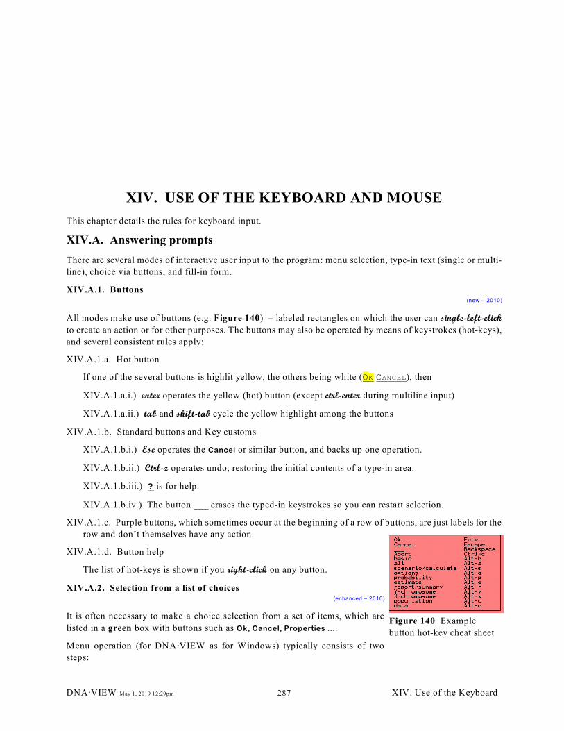
XIV. USE OF THE KEYBOARD AND MOUSE
This chapter details the rules for keyboard input.
XIV.A. Answering prompts
There are several modes of interactive user input to the program: menu selection, type-in text (single or multi-
line), choice via buttons, and fill-in form.
XIV.A.1. Buttons(new – 2010)
All modes make use of buttons (e.g. Figure 140) – labeled rectangles on which the user can single-left-click
to create an action or for other purposes. The buttons may also be operated by means of keystrokes (hot-keys),
and several consistent rules apply:
XIV.A.1.a. Hot button
If one of the several buttons is highlit yellow, the others being white (OK CANCEL), then
XIV.A.1.a.i.) enter operates the yellow (hot) button (except ctrl-enter during multiline input)
XIV.A.1.a.ii.) tab and shift-tab cycle the yellow highlight among the buttons
XIV.A.1.b. Standard buttons and Key customs
XIV.A.1.b.i.) Esc operates the Cancel or similar button, and backs up one operation.
XIV.A.1.b.ii.) Ctrl-z operates undo, restoring the initial contents of a type-in area.
XIV.A.1.b.iii.) ? is for help.
XIV.A.1.b.iv.) The button ___ erases the typed-in keystrokes so you can restart selection.
XIV.A.1.c. Purple buttons, which sometimes occur at the beginning of a row of buttons, are just labels for the
row and don’t themselves have any action.
XIV.A.1.d. Button help
The list of hot-keys is shown if you right-click on any button.
XIV.A.2. Selection from a list of choices(enhanced – 2010)
It is often necessary to make a choice selection from a set of items, which are
listed in a green box with buttons such as Ok, Cancel, Properties ....
Menu operation (for DNA@VIEW as for Windows) typically consists of two
steps:
Figure 140 Example
button hot-key cheat sheet
DNA@VIEW May 1, 2019 12:29pm XIV. Use of the Keyboard287
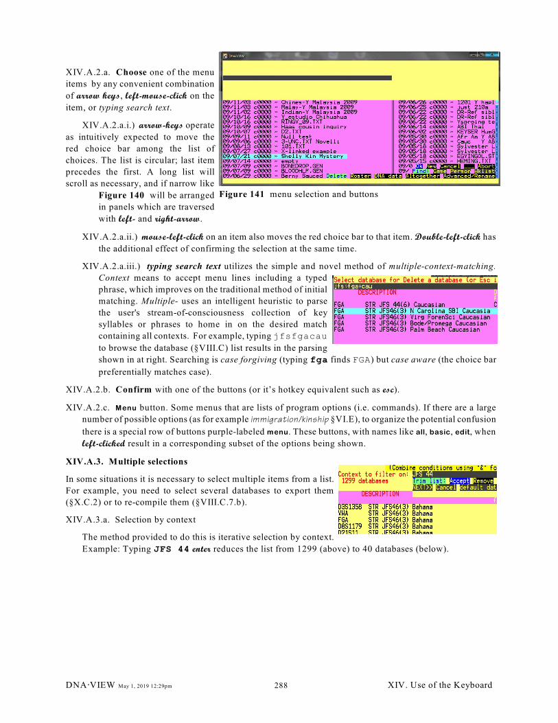
Figure 141 menu selection and buttons
XIV.A.2.a. Choose one of the menu
items by any convenient combination
of arrow keys, left-mouse-click on the
item, or typing search text.
XIV.A.2.a.i.) arrow-keys operate
as intuitively expected to move the
red choice bar among the list of
choices. The list is circular; last item
precedes the first. A long list will
scroll as necessary, and if narrow like
Figure 140 will be arranged
in panels which are traversed
with left- and right-arrow.
XIV.A.2.a.ii.) mouse-left-click on an item also moves the red choice bar to that item. Double-left-click has
the additional effect of confirming the selection at the same time.
XIV.A.2.a.iii.) typing search text utilizes the simple and novel method of multiple-context-matching.
Context means to accept menu lines including a typed
phrase, which improves on the traditional method of initial
matching. Multiple- uses an intelligent heuristic to parse
the user's stream-of-consciousness collection of key
syllables or phrases to home in on the desired match
containing all contexts. For example, typing jfsfgacau
to browse the database (§VIII.C) list results in the parsing
shown in at right. Searching is case forgiving (typing fga finds FGA) but case aware (the choice bar
preferentially matches case).
XIV.A.2.b. Confirm with one of the buttons (or it’s hotkey equivalent such as esc).
XIV.A.2.c. Menu button. Some menus that are lists of program options (i.e. commands). If there are a large
number of possible options (as for example immigration/kinship §VI.E), to organize the potential confusion
there is a special row of buttons purple-labeled menu. These buttons, with names like all, basic, edit, when
left-clicked result in a corresponding subset of the options being shown.
XIV.A.3. Multiple selections
In some situations it is necessary to select multiple items from a list.
For example, you need to select several databases to export them
(§X.C.2) or to re-compile them (§VIII.C.7.b).
XIV.A.3.a. Selection by context
The method provided to do this is iterative selection by context.
Example: Typing JFS 44 enter reduces the list from 1299 (above) to 40 databases (below).
DNA@VIEW May 1, 2019 12:29pm XIV. Use of the Keyboard288
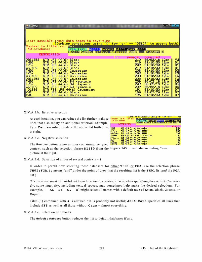
Figure 145 ... and also including Cauc
XIV.A.3.b. Iterative selection
At each iteration, you can reduce the list further to those
lines that also satisfy an additional criterion. Example:
Type Caucas enter to reduce the above list further, as
at right.
XIV.A.3.c. Negative selection
The Remove button removes lines containing the typed
context, such as the selection phrase D1S80 from the
picture at the right.
XIV.A.3.d. Selection of either of several contexts – &
In order to permit now selecting those databases for either TH01 or FGA, use the selection phrase
TH01&FGA. (& means “and” under the point of view that the resulting list is the TH01 list and the FGA
list.)
Of course you must be careful not to include any inadvertent spaces when specifying the context. Convers-
ely, some ingenuity, including textual spaces, may sometimes help make the desired selections. For
example, “ A& B& C& H” might select all names with a default race of Asian, Black, Caucas, or
Hispan.
Tilde (~) combined with & is allowed but is probably not useful; JFS&~Cauc specifies all lines that
include JFS as well as all those without Cauc – almost everything.
XIV.A.3.e. Selection of defaults
The default databases button reduces the list to default databases if any.
DNA@VIEW May 1, 2019 12:29pm XIV. Use of the Keyboard289
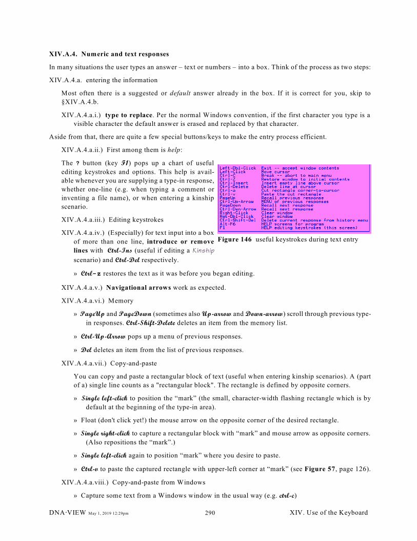
Figure 146 useful keystrokes during text entry
XIV.A.4. Numeric and text responses
In many situations the user types an answer – text or numbers – into a box. Think of the process as two steps:
XIV.A.4.a. entering the information
Most often there is a suggested or default answer already in the box. If it is correct for you, skip to
§XIV.A.4.b.
XIV.A.4.a.i.) type to replace. Per the normal Windows convention, if the first character you type is a
visible character the default answer is erased and replaced by that character.
Aside from that, there are quite a few special buttons/keys to make the entry process efficient.
XIV.A.4.a.ii.) First among them is help:
The ? button (key F1) pops up a chart of useful
editing keystrokes and options. This help is avail-
able whenever you are supplying a type-in response,
whether one-line (e.g. when typing a comment or
inventing a file name), or when entering a kinship
scenario.
XIV.A.4.a.iii.) Editing keystrokes
XIV.A.4.a.iv.) (Especially) for text input into a box
of more than one line, introduce or remove
lines with Ctrl-Ins (useful if editing a Kinship
scenario) and Ctrl-Del respectively.
» Ctrl-z restores the text as it was before you began editing.
XIV.A.4.a.v.) Navigational arrows work as expected.
XIV.A.4.a.vi.) Memory
» PageUp and PageDown (sometimes also Up-arrow and Down-arrow) scroll through previous type-
in responses. Ctrl-Shift-Delete deletes an item from the memory list.
» Ctrl-Up-Arrow pops up a menu of previous responses.
» Del deletes an item from the list of previous responses.
XIV.A.4.a.vii.) Copy-and-paste
You can copy and paste a rectangular block of text (useful when entering kinship scenarios). A (part
of a) single line counts as a "rectangular block". The rectangle is defined by opposite corners.
» Single left-click to position the “mark” (the small, character-width flashing rectangle which is by
default at the beginning of the type-in area).
» Float (don't click yet!) the mouse arrow on the opposite corner of the desired rectangle.
» Single right-click to capture a rectangular block with “mark” and mouse arrow as opposite corners.
(Also repositions the “mark”.)
» Single left-click again to position “mark” where you desire to paste.
» Ctrl-v to paste the captured rectangle with upper-left corner at “mark” (see Figure 57, page 126).
XIV.A.4.a.viii.) Copy-and-paste from Windows
» Capture some text from a Windows window in the usual way (e.g. ctrl-c)
DNA@VIEW May 1, 2019 12:29pm XIV. Use of the Keyboard290
» Left click in the DNA@VIEW window into which you wish to paste and position the insertion mark.
» Right-click on the title bar (the strip at the top) of the DNA@VIEW window, put the cursor on the
word Edit, slide out to Paste and click.
XIV.A.4.a.ix.) Insert/replace mode: The insert toggles as would be expected between insert and replace
modes. Also, the cursor height reflects the mode to give you visual feedback: Thin cursor=insert, thick
cursor=replace.
XIV.A.4.b. termination character to confirm the input
Completion of entry into those fields requiring a number(s) or text as an answer is usually signaled by
striking Enter. If only one number is expected, then Space is usually allowed also. In some cases, Tab or
a letter (a role letter signals exit from the “year” part of an accession number) may suffice; see the
instructions. To conclude entering a kinship scenario (§VI.F.1), Esc.
XIV.A.5. Entering probabilities
A probability is a number in the range 0 to 1 inclusive. For convenience a few shortcuts are implemented:
XIV.A.5.a. Entering a number >1 is allowed, and it will be interpreted as either a percent, or a reciprocal.
Example:
Use what prior? (0!1; 0 means “none”): 999
Do you mean (a)99.9% (b)1/999 (c)neither? a
XIV.A.5.b. The NONE button indicates no probability. For example pick NONE for prior probability to avoid any
posterior probability computation. Entering probability=0 has the same effect.
XIV.A.6. Yes/No prompts
Answer y or n. Synonyms for yes include j, s, and o. Do NOT also strike Enter. However, if a default
answer such as y is already sitting in the answer box, then it is ok to Enter to accept the suggestion.
XIV.A.7. Dates
Dates are input as month, day, year (for the US — other orders as conventional in other parts of the world)
with today’s date usually presented as the default. The month is accepted as a choice (§XIV.A.2, page 287)
from a list of the months; day and year are numeric input (§XIV.A.4, page 290). Terminate selection for each
field with Space to continue to the next field; terminate with Enter or Tab to accept the remaining default
choices. To back up and correct mistakes, the keys left arrow (previous field) and home (start over) are
supported.
Accession dates are used only for documentation. If they don’t interest you, the option §IX.E.4 can save a little
time.
XIV.A.8. Mouse input methods
XIV.A.8.a. Menu selection
Double click on a menu choice to select it, or double click outside of the green choice area to select the
currently highlighted item.
Single click on a menu choice to highlight it, or single click outside of the green choice area to clear the
highlighting.
You can click on the scroll bar to scroll, or on find or clear or help for those tasks.
DNA@VIEW May 1, 2019 12:29pm XIV. Use of the Keyboard291
XIV.A.8.b. Yes/No questions:
Double left click for yes.
Double right click for no.
XIV.A.8.c. Questions requiring Numeric or Text response:
Double left click to accept the suggested default.
XIV.A.8.d. Within Help Screens:
Left click to select a help menu choice.
Right click to back up a help screen.
XIV.A.9. People
People are described by an accession number, a race, and an accession date. Any place that a person entry is
called for, a new person may be defined, or the race and accession date can be corrected.
XIV.A.9.a. Editing the Accession Number
The accession number is in two parts, separated by -. The first part is up to four digits, and may be used
as a year code (e.g. 91 or 2000). Type - or space to advance to the second part, which is up to five digits.
Leading zeros are not significant. The “year part” is not allowed to be 0. Thus, 2000!0 is allowed but
0-1 is not allowed.
There is no requirement to use the leading part of the accession number to indicate the year — it is just
a scheme that many labs do use.
Terminate the accession number entry with Enter (OK) skip editing the race and accession date, or with
Space if you wish to edit either race or accession date. However, if the person is previously undefined you
will not be allowed to skip.
XIV.A.9.a.i.) Home backs up from the middle to the beginning of entry for a person.
XIV.A.9.a.ii.) Two and four digit year numbers
Until the year 1999, DNA·VIEW only allowed two digits for the year number, eliding the century
part. So you would enter 98!12345. The extra two digits are necessary in order to maintain the
“year!sequence” scheme into the year 2000 and beyond.
The addition of the extra digits introduces possible ambiguity and confusion between pairs of numbers
like 98!12345 and 1998!12345. DNA·VIEW handles this possible ambiguity as follows:
» 98!12345 and 1998!12345 are not the same — they are two separate people.
» If you type one of them — say 1998!12345 — and it does not exist, but the other one — 98!12345
in this case does exist, you will be warned, and given an opportunity to change your mind. A pop-
up box prompts:
There already is a 98!12345
and the choice box offers the choices:
Then please use the old number: 98!12345
Create 1998!12345 anyway. We’ll have both numbers.
DNA@VIEW May 1, 2019 12:29pm XIV. Use of the Keyboard292
with the first of those choices the default, already highlighted. Thus, hit enter if you made a
mistake and want to use the number that already exists. Type Center to insist on creating the
alternate number.
XIV.A.9.a.iii.) Accession/sample number lookup by case
Very often when you want to enter an accession number the most convenient method is to copy it from
a case in which the sample occurs.
At the accession number input dialogue, click COPY FROM A CASE. Or in the particular case of entering
roster data in a worklist, put the red bounce bar on the lane to populate and click COPY FROM: CASE.
Either way, the From case? dialogue pops up. Enter the case number (the RECENT or SEARCH
buttons may be helpful), then at Copy whom? choose the desired sample.
XIV.A.9.b. Editing the race code
The race is a single letter, or ! (used for children) (§IX.A.4, page 197). If you type ?, then you can see
and edit the list of race names. You may select any race letter desired with OK, and the PROPERTIES button
lets you enter or change any race name.
XIV.A.9.c. The accession date
The accession date is entered and edited as described in §XIV.A.7.
The accession date is printed along with the other accession fields on the case report, but has no
importance at present in DNA·VIEW. Therefore it is reasonable to accept always the default, which is
today’s date.
XIV.A.10. Case numbering
Parentage, kinship, and crime cases are referenced by number.
The case number must be a positive integer up to about 2,147,000,000. Sorry, nothing but digits are allowed
– no spaces, letters, dashes, superscripts, dots, colors, italics, or Sumerian cuneiform marks although there is
some flexibility in specifying a format for the number (§IX.F.2).
Several features make case number entry more convenient including popup memory of “popular cases” and
keystroke shortcuts for automatically prefixing the year. See §IX.F.2 and §V.B.28.a.iii.
DNA@VIEW May 1, 2019 12:29pm XIV. Use of the Keyboard293
XIV.B. Special Editing Screen
In a few rare situations – when some DNA@VIEW operation requires editing a large block of text – the editing
takes place in a special editing screen with its own special rules.
You can tell that you are in the special editing screen if either
(i) There are bracketed numbers – e.g.
[0][1][2]
along the left margin of the screen, or
(ii) such numbers appear after you type ctrl-o. (Ctrl-o again to toggle the numbers off.)
The basic rules for editing are these:
XIV.B.1. Navigating
< You may use the cursor arrows or Enter to move about.
< You may use the Ctrl-cursor arrows, and PgUp, PgDn, Home, End, with or without Ctrl, to move about
faster.
XIV.B.2. Input. There is a text full-screen editor, and a numeric one (used for editing probabilities).
XIV.B.2.a. Text input
< Type in the normal manner.
< The Ins key toggles between insert and replace modes.
XIV.B.2.b. Numeric input
< Navigate to the cell to change. Type in a number, which appears at the bottom of the screen.
< Type Enter or any other navigation instruction to enter the number into the cell.
XIV.B.3. Deleting and Inserting
< Del and Backspace delete at and behind the cursor.
< Alt-F4 deletes a line. Alt-F3 inserts a line. Use these options with great restraint. There is no harm in
reordering the list of readers, but it is important that each probe and each restriction enzyme retain its
line number.
< Add a line at the bottom with Enter (from the last previous line).
< Add a new column (numeric input only, and it should never be necessary) with Alt-Enter.
XIV.B.4. Exit
< Ctrl-F5 or Ctrl-e to file the changes when done.
< Ctrl-q to quit and abort the changes.
XIV.B.5. Miscellaneous
< Ctrl-o toggles the line numbers on and off.
< Ctrl-h may get a help screen, but this is not guaranteed
DNA@VIEW May 1, 2019 12:29pm XIV. Use of the Keyboard294
XV. APPENDIX — INSTALLATION AND UPDATE
XV.A. Installation
The computer must be a PC, a Pentium for example. Mac with a Windows emulator doesn't work.
DNA·VIEW consists of one CD, or a file obtained from the Internet. The installation file has a name like
SetupDNAVIEW....EXE. If using an installation CD, setup should autostart, but you can browse to the file
(My Computer etc.) and click on it if not.
The installation procedure is
XV.B. Preliminary for network installation
XV.B.1. For installation to a network server,
note that there must be a mapped drive letter designating (part of) a shared folder. See the DNA@VIEW manual
§XVI.D Also, users must have permission to change and create files in the server folder .
XV.B.1.a. Example: Install to \\server-1
» Create or choose a shared folder such as \\server-1\DNA, sharename=sDNA for example.
» Grant full access to sDNA to all DNA@VIEW users.
» Map network drive: Choose a drive letter e.g. X: and on every workstation that uses DNA@VIEW
(including \\server-1), map X: ] \\server-1\sDNA.
Use the same drive letter, e.g. X:, on every workstation.
XV.C. Begin installation
Answer the prompts.
XV.C.1. Password
There may or may not be a password.
XV.C.2. Select Destination Location
XV.C.2.a. If updating, choose the directory where DNA@VIEW already is.
WARNING: Sometimes the installer suggests a location with an extra “dnaview”, such as
C:\dnaview\dnaview. Don’t be fooled!
XV.C.2.b. For a new installation, anywhere you like. Examples:
XV.C.2.b.i.) Traditionally DNA@VIEW was installed to C:\dnaview.
DNA@VIEW May 1, 2019 12:29pm XV. Appendix – Installation295
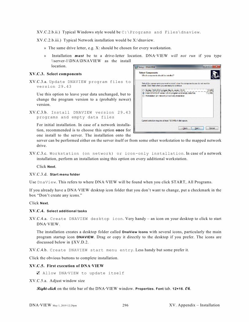
XV.C.2.b.ii.) Typical Windows style would be C:\Programs and Files\dnaview.
XV.C.2.b.iii.) Typical Network installation would be X:\dnaview.
» The same drive letter, e.g. X: should be chosen for every workstation.
» Installation must be to a drive-letter location. DNA@VIEW will not run if you type
\\server-1\DNA\DNAVIEW as the install
location.
XV.C.3. Select components
XV.C.3.a. Update DNAVIEW program files toversion 29.43
Use this option to leave your data unchanged, but to
change the program version to a (probably newer)
version.
XV.C.3.b. Install DNAVIEW version 29.43programs and empty data files
For initial installation. In case of a network installa-
tion, recommended is to choose this option once for
one install to the server. The installation onto the
server can be performed either on the server itself or from some other workstation to the mapped network
drive.
XV.C.3.c. Workstation (on network) or icon-only installation. In case of a network
installation, perform an installation using this option on every additional workstation.
Click Next.
XV.C.3.d. Start menu folder
Use DnaView. This refers to where DNA@VIEW will be found when you click START, All Programs.
If you already have a DNAAVIEW desktop icon folder that you don’t want to change, put a checkmark in the
box “Don’t create any icons.”
Click Next.
XV.C.4. Select additional tasks
XV.C.4.a. Create DNAVIEW desktop icon. Very handy – an icon on your desktop to click to start
DNA@VIEW.
The installation creates a desktop folder called DnaView Icons with several icons, particularly the main
program startup icon DNAVIEW. Drag or copy it directly to the desktop if you prefer. The icons are
discussed below in §XV.D.2.
XV.C.4.b. Create DNAVIEW start menu entry. Less handy but some prefer it.
Click the obvious buttons to complete installation.
XV.C.5. First execution of DNA@VIEW
~T Allow DNA@VIEW to update itself
XV.C.5.a. Adjust window size
Right-click on the title bar of the DNA@VIEW window. Properties. Font tab. 12×16. Ok.
DNA@VIEW May 1, 2019 12:29pm XV. Appendix – Installation296
On Windows XP or older you can also invoke full-screen mode via alt-enter.
XV.C.6. Install Pater
If installing PATER as well as DNA@VIEW, running the PATER installer – SetupPATER....EXE on the
same CD – is a separate operation. Use My Computer to double-click on the installer to run it.
XV.D. Networking
If you will operate DNA@VIEW from several workstations at the same time, you must establish the network
protocol so that when two instances of the program running on two different machines need to write
information to the same file they will cooperatively take turns.
XV.D.1. Turn on networking
XV.D.1.a. Open DNA@VIEW on a first workstation (can be the server itself) and
Housekeeping < Maintenance < network preferences
Do you want to make it networked? YES
Which protocol? LOCALSHARE (try this one first).
Name for this workstation? Octopus Save (a name representing the DNAVIEW installation)
NETWORK LOCK TEST. Now leave the first workstation and enroll a second one to continue the test.
XV.D.1.b. On a second workstation (and additional workstations can be added as needed)
XV.D.1.b.i.) (optional, and see §XI.D.1.a) Copy X:\dnaview\DNACFG.SF to exactly C:\dnaview\DNACFG.
SF.25
This allows the workstation to have its individual name and a few other parameters of its own.
» Housekeeping < Maintenance < network preferences
CHANGE: NAME. Name for this workstation: Anthill OK
Note: The network and any workstation without its own C:\dnaview\DNACFG.SF will have a workstation
name Octopus, or Octopus1, etc. CHANGE NAME from such a workstation would change the network
name (from Octopus).
XV.D.1.b.ii.) Continue the network lock test, with the first workstation still waiting:
Housekeeping < Maintenance < network preferences. NETWORK LOCK TEST
That’s the default. If you really want it somewhere else, specify the folder in X:\dnaview\dnaview.ini,25
[config] section, LCFGFolder= parameter.
DNA@VIEW May 1, 2019 12:29pm XV. Appendix – Installation297
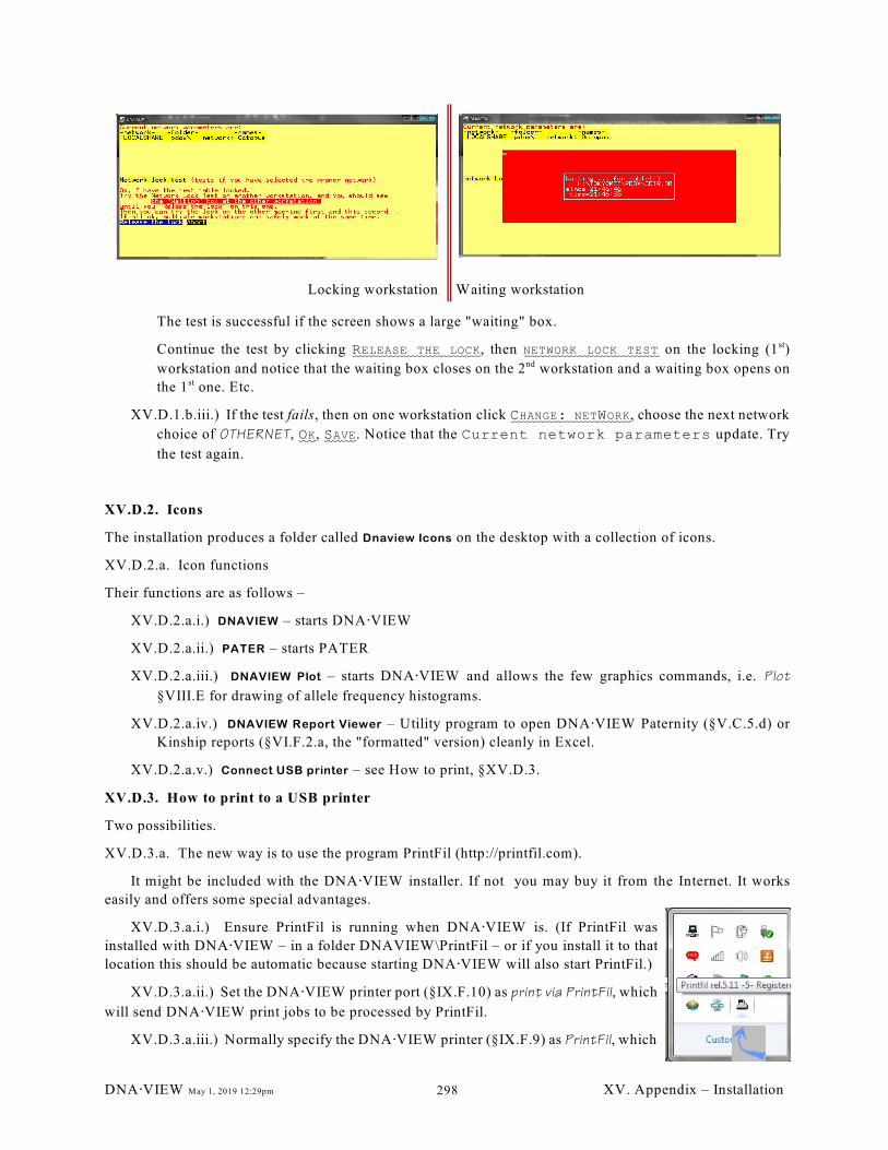
Locking workstation Waiting workstation
The test is successful if the screen shows a large "waiting" box.
Continue the test by clicking RELEASE THE LOCK, then NETWORK LOCK TEST on the locking (1 )st
workstation and notice that the waiting box closes on the 2 workstation and a waiting box opens onnd
the 1 one. Etc.st
XV.D.1.b.iii.) If the test fails, then on one workstation click CHANGE: NETWORK, choose the next network
choice of OTHERNET, OK, SAVE. Notice that the Current network parameters update. Try
the test again.
XV.D.2. Icons
The installation produces a folder called Dnaview Icons on the desktop with a collection of icons.
XV.D.2.a. Icon functions
Their functions are as follows –
XV.D.2.a.i.) DNAVIEW – starts DNA@VIEW
XV.D.2.a.ii.) PATER – starts PATER
XV.D.2.a.iii.) DNAVIEW Plot – starts DNA@VIEW and allows the few graphics commands, i.e. Plot
§VIII.E for drawing of allele frequency histograms.
XV.D.2.a.iv.) DNAVIEW Report Viewer – Utility program to open DNA@VIEW Paternity (§V.C.5.d) or
Kinship reports (§VI.F.2.a, the "formatted" version) cleanly in Excel.
XV.D.2.a.v.) Connect USB printer – see How to print, §XV.D.3.
XV.D.3. How to print to a USB printer
Two possibilities.
XV.D.3.a. The new way is to use the program PrintFil (http://printfil.com).
It might be included with the DNA@VIEW installer. If not you may buy it from the Internet. It works
easily and offers some special advantages.
XV.D.3.a.i.) Ensure PrintFil is running when DNA@VIEW is. (If PrintFil was
installed with DNA@VIEW – in a folder DNAVIEW\PrintFil – or if you install it to that
location this should be automatic because starting DNA@VIEW will also start PrintFil.)
XV.D.3.a.ii.) Set the DNA@VIEW printer port (§IX.F.10) as print via PrintFil, which
will send DNA@VIEW print jobs to be processed by PrintFil.
XV.D.3.a.iii.) Normally specify the DNA@VIEW printer (§IX.F.9) as PrintFil, which
DNA@VIEW May 1, 2019 12:29pm XV. Appendix – Installation298
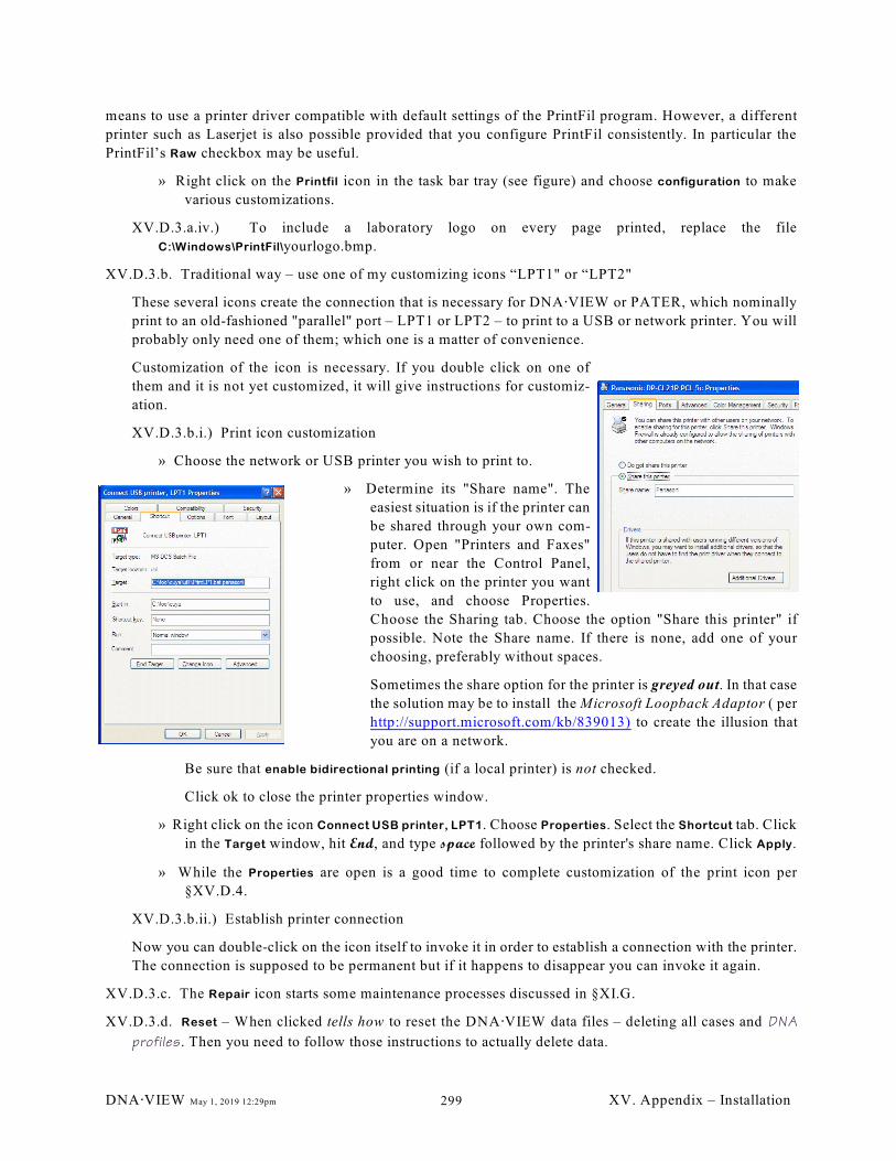
means to use a printer driver compatible with default settings of the PrintFil program. However, a different
printer such as Laserjet is also possible provided that you configure PrintFil consistently. In particular the
PrintFil’s Raw checkbox may be useful.
» Right click on the Printfil icon in the task bar tray (see figure) and choose configuration to make
various customizations.
XV.D.3.a.iv.) To include a laboratory logo on every page printed, replace the file
C:\Windows\PrintFil\yourlogo.bmp.
XV.D.3.b. Traditional way – use one of my customizing icons “LPT1" or “LPT2"
These several icons create the connection that is necessary for DNA@VIEW or PATER, which nominally
print to an old-fashioned "parallel" port – LPT1 or LPT2 – to print to a USB or network printer. You will
probably only need one of them; which one is a matter of convenience.
Customization of the icon is necessary. If you double click on one of
them and it is not yet customized, it will give instructions for customiz-
ation.
XV.D.3.b.i.) Print icon customization
» Choose the network or USB printer you wish to print to.
» Determine its "Share name". The
easiest situation is if the printer can
be shared through your own com-
puter. Open "Printers and Faxes"
from or near the Control Panel,
right click on the printer you want
to use, and choose Properties.
Choose the Sharing tab. Choose the option "Share this printer" if
possible. Note the Share name. If there is none, add one of your
choosing, preferably without spaces.
Sometimes the share option for the printer is greyed out. In that case
the solution may be to install the Microsoft Loopback Adaptor ( per
http://support.microsoft.com/kb/839013) to create the illusion that
you are on a network.
Be sure that enable bidirectional printing (if a local printer) is not checked.
Click ok to close the printer properties window.
» Right click on the icon Connect USB printer, LPT1. Choose Properties. Select the Shortcut tab. Click
in the Target window, hit End, and type space followed by the printer's share name. Click Apply.
» While the Properties are open is a good time to complete customization of the print icon per
§XV.D.4.
XV.D.3.b.ii.) Establish printer connection
Now you can double-click on the icon itself to invoke it in order to establish a connection with the printer.
The connection is supposed to be permanent but if it happens to disappear you can invoke it again.
XV.D.3.c. The Repair icon starts some maintenance processes discussed in §XI.G.
XV.D.3.d. Reset – When clicked tells how to reset the DNA@VIEW data files – deleting all cases and DNA
profiles . Then you need to follow those instructions to actually delete data.
DNA@VIEW May 1, 2019 12:29pm XV. Appendix – Installation299
XV.D.4. Customizing the icons
There are a few detailed icon option settings that it was not possible to incorporate into the installer. Therefore
for best performance and appearance I suggest the following steps, for each icon that you will use:
XV.D.4.a. Right click an icon and choose properties
XV.D.4.a.i.) font/window size
» Click the font tab and choose a font of comfortable size, such as font: raster font and font size: 12 x
16.
» Click the options tab. Under Display options click on the Windows radial button.
» Click the layout tab and make sure that Window size is 80 and 25.
XV.D.4.a.ii.) enable mouse for menu. Click the options tab and make sure that Quick edit mode is not
checked.
XV.D.5. Start DNA·VIEW
Execute (or allow to execute) the command Update (§XI.B) from the Housekeeping menu.
XV.D.6. Graphics checkout
Start DNA@VIEW using the special DNAVIEW PLOT icon.
Select Plot, choose any database, and hit Enter to select all the default choices until DISPLAY. You should now
see a graph on the screen.
If not, exit from DNA@VIEW and examine the file \DNAVIEW\GSS\CGI.CFG with a text editor (WordPad
will do). Look at the file CGI.CFG and compare what you see with the contents of the directory. Are there
perhaps incorrect drive letters mentioned in CGI.CFG, out-of-date paths, or missing files? Are there any error
messages when you start up DNA·VIEW? Call for help.
If DISPLAY works, hit Enter to end the display, and choose PRINTER. A similar picture should appear on the
printer.
XV.D.7. Mouse checkout.
The (little-used) commands PCR Read , and Import/Export gel image require a special mouse driver. For
documentation, obtain an old DNA@VIEW manual from the Internet.
XV.D.8. De-installing a DNA·VIEW System Update
XV.D.8.a. Backup subdirectories
Before installing a new program version it is advisable to save the old one. The essential files to save are
the program files DNATREE*.SF, DNAVIEW.WS and the configuration data files DNACFG.SF,
DNAMAINT.SF, all from the installation folder of DNAAVIEW such as C:\DNAVIEW. (Don’t worry
about anything in the UPDATES folder.)
Earlier versions of the DNAAVIEW update routine automatically sequestered these files in folders named
e.g. C:\DNAVIEW\PRE27.12 (if the new version is 27.12). You can delete these subdirectories once
you feel you will not need them.
XV.D.8.b. Retreating to a previous version
So long as the old and new version numbers have the same integer part (e.g. 27.04 and 27.12), you can
retreat just by copying back the files DNATREE*.SF and DNAVIEW.WS.
DNA@VIEW May 1, 2019 12:29pm XV. Appendix – Installation300
If the old and new version numbers are farther apart, then it depends, so please call DNA·VIEW for
special instructions. If you wish to retreat and have NOT already run the DNA·VIEW Update command
(§XVI.B.1.i.iii), then don’t run it.
XV.D.9. Installing Frequency databases
Allele population frequencies ("databases") are included when DNAAVIEW is initially installed. Additional
databases can be added in a variety of ways (the Import/Export command options described in §X.C and
§X.B). Use the method of §X.C.1 to merge databases into the active DNA@VIEW library from a source in
proprietary DNA@VIEW format:
XV.D.9.a. Distributed of DNA@VIEW frequency databases
Large files of frequency databases are included on distribution CD's including the update CD's that are
distributed yearly. They are in the \FREQ folder.
XV.D.9.b. Importing DNA·VIEW frequency databases from another user
DNA·VIEW users can trade frequency databases by using the Import/Export command options described
in §X.C.
XV.D.10. Installation — Check
XV.D.10.a. Graphic printing
Check that \dnaview\CGI.CFG mentions the correct printer driver. If not, you won’t be able to print
graphs. Other reports aren’t affected.
XV.D.10.b. Numlock status
See §IX.F.24 for the Option to toggle the numlock status.
XV.D.10.c. Printing
See §IX.F.9 and §IX.F.10 for Options to specify the printer and the printer port, and §XV.D.2.a.v for
printing under Windows.
XV.D.10.d. Extended or expanded memory for DNA@VIEW under Windows
Especially if you experience a WS FULL error message from DNAAVIEW, edit the file (Notepad,
Microsoft Word, or any text editor will do, but be sure to re-save as “Text”!)
\DNAVIEW\APLII\CONFIG.APL and check the wssize= line. The number is the number of
kilobytes of RAM that DNAAVIEW will be allocated.
wssize=100000
is a modest allocation (representing 100 megabytes) considering the amount of memory most computers
have available. The minimum is about 5000; the maximum is about 500000 (half a gigabyte).
XV.D.10.e. File handles
DNAAVIEW requires at least 70 of a system resource called “file handles.” Otherwise the program may
produce an error message Not enough file handles.
XV.D.10.e.i.) Windows XP etc.
DNA@VIEW May 1, 2019 12:29pm XV. Appendix – Installation301
Ensure the FILES= line is at least FILES=70 in a file called Config.NT. There is a sample
version of Config.NT, with sufficient file handles specified, in the directory where DNAVIEW is
installed (possibly named C:\DNAVIEW.)
The normal copy of Config.NT is located in the system directory — usually at
\Windpws\System32\Config.NT, but more generally at the symbolic location
\%systemroot%\System32\Config.NT. It may be invisible. You need administrative rights
to change it. Even some administrators are unaware of it, but it is there!
XV.D.10.f. Windows XP/NT/2000 startup glitch
Starting DNAAVIEW or PATER under Windows XP may produce a pop-up window with the message:
16 bit MS-DOS Error
The system cannot open COM1 port requested by the application. Click 'Close' to terminate
the application
Click 'Ignore' and the program will start ok. To avoid the message altogether, examine two files:
XV.D.10.f.i.) In dnaview\aplii\config.apl there is probably an !----- Environment
Information section (! indicates a comment line) followed by an Env= line.
Change Env=2 or Env=258 to Env=18.
Change Env=0 or Env=256 to Env=16.
XV.D.10.f.ii.) In dnaview\dnaview.bat, change any E2 or E256 or similar phrase at the end of the
line (near the end of the file) that includes APLPDX according to the same pattern. (This will apply
only to an old installation of DNA@VIEW.)
XV.D.11. Printing from DNAAVIEW (in Windows)
Printing from DNAAVIEW or PATER when running under Windows may require a trick.
XV.D.11.a. Printing to an LPT port
DNA@VIEW only knows how to print to LPT1 or LPT2 (§IX.F.10), which are traditional names for plugs
on the back of the computer where printers used to be plugged in. DNA@VIEW sends messages to one of
these old-fashioned port names in order to print. Windows needs to be told somehow to intercept and
re-route all such messages. If the printer is physically plugged into LPT1 (or LPT2) on the local machine,
there is no problem. Just tell DNAAVIEW or PATER to print to that port.
A small complication arises when the printer is a network printer and/or a USB printer, which is the usual
arrangement these days. Therefore, to print it may be necessary to ask Windows to intercept LPT messages
and re-route them to the actual printer. How to do this depends on the version of Windows.
XV.D.11.b. Printing to a network or USB printer from Windows XP (2000, NT, Vista)
See Connect USB printer, §XV.D.2.a.v. (For the technically inclined, it invokes a NET USE command.)
XV.D.11.c. Printing to a network or USB printer from Windows 98
In Windows 98 there is a “capture printer port” option on the printer properties window. Use it to ask
Windows to re-route any requests for the port to which you elect (§IX.F.10 – e.g. LPT1) to print. to the
specified printer:
Double click on My Computer
Double click on the Printers Folder
DNA@VIEW May 1, 2019 12:29pm XV. Appendix – Installation302
Click on Printer
Click on Properties
Click on the Details Tab (the tabs are at the top of the current window)
Click on Capture Printer Port Button
Set the device as LPT1, or whatever you selected as §IX.F.10.
Choose the path for the desired printer – e.g. \\YourServerName\PrinterName
Check "Reconnect at logon"
Click on OK
XV.E. Running DNA@VIEW under Windows
DNA@VIEW will run under 32 bit Windows 7 or earlier in an ordinary DOS box. If you are stuck with 64-bit
operating systems, documentation for running in Virtual PC or under DOSbox can be supplied on request.
XV.E.1. Startup
Usually click the DNAVIEW icon or choose DNA@VIEW from the start menu.
XV.E.2. Hardware security key
If you have a hardware security key, it must be plugged into a USB port. In case of a network installation, the
port must be on some accessible computer such as the server on which DNA@VIEW is installed.
XV.E.3. Startup with graphics
To start DNA@VIEW in an enhanced mode that enables a few special DNA @VIEW commands such as Plot
(§171), use the special icon DNAVIEW PLOT. It will only run on Windows XP or below.
Unfortunately this mode comes at a small price – a Windows XP / DOS process priority conflict that causes
DNA@VIEW to play badly with other Windows processes. Even printing from DNA-VIEW takes15 seconds.
XV.E.3.a. A basic fix – Lowering priority of DNA@VIEW in Windows
XV.E.3.a.i.) Start Windows' Task Manager (While holding Ctrl-Alt, hit Del). Click the "Processes" tab.
XV.E.3.a.ii.) Start DNAVIEW PLOT.
XV.E.3.a.iii.) Click on the Task Manager.
» Find the DOS process, e.g. by hitting n repeatedly. It will be called ntvdm.exe. Right click on
it.
» From the fly-out, choose Set Priority
» From the next fly-out, click on Below Normal
» Close the Task Manager with the X.
This change is temporary, lasting only until you close DNA@VIEW.
XV.E.4. Annoying message
If, when trying to start DNAAVIEW/Toolbox, Windows complains about COM1 and asks " Close or Ignore?",
click "Ignore" and everything will work fine. This probably only happens on older DNA@VIEW installations.
See §XV.D.10.f for the fix.
XV.E.4.a. Windows Lore. Did you know?
DNA@VIEW May 1, 2019 12:29pm XV. Appendix – Installation303
When DNA·VIEW is running, you can use alt-enter to toggle between full- and windowed- screen.
Alt-tab cycles among running Windows processes, including DNA·VIEW.
XV.E.4.a.i.) What is that funny Flying-Windows key good for?
The flying-windows key brings up the desktop and the Start menu.
Flying-window+D clears away all windows. Do it again to bring them back.
Flying-window+M minimizes all windows. Flying-window+shift-M to restore them.
Flying-window+E opens the Windows Explorer (i.e. “My Computer”)
Flying-window+R opens the Run dialogue.
XV.E.4.a.ii.) Host Access Error
In the process of transmitting files from one computer to another there are various ways that the “Read
only” attribute can get turned on. For example, copying a file from a CD usually has this result. If
DNAAVIEW or PATER then tries to write to that file, the result is the error message HOST ACCESS
ERROR. You can remove the read-only status and fix the problem by right-clicking on the file name
in Windows and changing the “properties”.
DNA@VIEW May 1, 2019 12:29pm XV. Appendix – Installation304
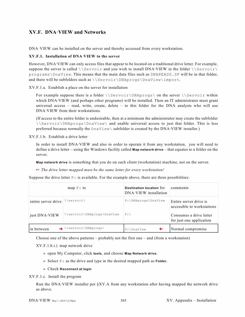
XV.F. DNA·VIEW and Networks
DNA·VIEW can be installed on the server and thereby accessed from every workstation.
XV.F.1. Installation of DNA@VIEW to the server
However, DNA@VIEW can only access files that appear to be located on a traditional drive letter. For example,
suppose the server is called \\Servoir and you wish to install DNA@VIEW in the folder \\Servoir\
programs\DnaView. This means that the main data files such as DNAREADS.SF will be in that folder,
and there will be subfolders such as \\Servoir\DNAprogs\DnaView\import.
XV.F.1.a. Establish a place on the server for installation
For example suppose there is a folder \\Servoir\DNAprogs\ on the server \\Servoir within
which DNA@VIEW (and perhaps other programs) will be installed. Then an IT administrator must grant
universal access – read, write, create, delete – to this folder for the DNA analysts who will use
DNA@VIEW from their workstations.
(If access to the entire folder is undesirable, then at a minimum the administrator may create the subfolder
\\Servoir\DNAprogs\DnaView\ and enable universal access to just that folder. This is less
preferred because normally the DnaView\ subfolder is created by the DNA@VIEW installer.)
XV.F.1.b. Establish a drive letter
In order to install DNA@VIEW and also in order to operate it from any workstation, you will need to
define a drive letter – using the Windows facility called Map network drive – that equates to a folder on the
server.
Map network drive is something that you do on each client (workstation) machine, not on the server.
L The drive letter mapped must be the same letter for every workstation!
Suppose the drive letter P: is available. For the example above, there are three possibilities:
map P: to Destination location for
DNA@VIEW installation
comments
entire server drive \\servoir\ P:\DNAprogs\DnaView Entire server drive is
accessible to workstations
just DNA@VIEW \\servoir\DNAprogs\DnaView P:\ Consumes a drive letter
for just one application
in between þ \\servoir\DNAprogs\ P:\DnaView ³ Normal compromise
Choose one of the above patterns – probably not the first one – and (from a workstation)
XV.F.1.b.i.) map network drive
» open My Computer, click tools, and choose Map Network drive.
» Select P: as the drive and type in the desired mapped path as Folder.
» Check Reconnect at login
XV.F.1.c. Install the program
Run the DNA@VIEW installer per §XV.A from any workstation after having mapped the network drive
as above.
DNA@VIEW May 1, 2019 12:29pm XV. Appendix – Installation305
XV.F.1.c.i.) Select the destination location (§XV.C.1) following an example from the table above.
That completes installation to the first workstation
XV.F.2. Install to other workstations
XV.F.2.a. Map network drive as above for the next workstation
XV.F.2.b. Create a startup icon on the desktop
This can be done by simply copying the icon folder from another workstation, or can be done with the
DNA@VIEW installation file (§XV.C.4).
XV.F.3. File sharing among workstations
When several users run DNA@VIEW at the same time, since they will all be sharing the same files containing
cases, DNA profiles, etc. it is important to have some kind of discipline to ensure that simultaneous writing
of information to the same file by different users doesn't cause the data files to become jumbled. Ideally the
software enforces the necessary discipline by some sort of file-locking mechanism .
Some of the DNA@VIEW data is stored in “APL” files (principally those with names of the DNA....SF) and
these files are automatically robust.
Other DNA@VIEW data is stored in “Paradox tables” and to ensure that they don't become inconsistent or even
corrupt some installation care is required.
XV.F.3.a. Network protocol
Use the Network preferences tool per §IX.A.8 to establish and check network operation.
XV.F.3.a.i.) Network details and comments
The most popular network is of course Novell (NE 2000 compliant cards), and DNA@VIEW seems to
work well with it. However, there are some oddities. Using Windows 95 I suggest choosing a “client
network component” of Microsoft client for NetWare networks, rather than Novell Client due to
early rumors of software problems (pre Feb 96, may be ok later) in the latter.
Similarly, in the Network preferences (§IX.A.8) includes a network option of NOVELLNET but in
practice LOCALSHARE sometimes works better.
The acid test is to try the Network Lock Test which the Network tool offers.
» Miscellaneous notes
Write-back caching can only mean trouble. Disable it.
One successful combination: “Windows Login loaded; IPS, NetBEUI (certainly used), TCP/IP
(presumably idle), NE 2000 compliant.”
Windows NT is not validated, but should work, since “APL environment switch env=18” —
jargon for a parameter setting in DNAVIEW.BAT.
OS/2 installations have worked.
MS-DOS protected mode DPMI. Auto. (I don’t know what this means, but wish to retain the
note!)
DNA@VIEW May 1, 2019 12:29pm XV. Appendix – Installation306
XV.F.4. Cloned DNA@VIEW on a network
When DNA@VIEW is added to various workstations as described above, all users on the network will access
the printer in the same way, will have the same report title on printed reports, will share memory for things
like the most recent DNA odds worksheet, and so on. Workstation names will vary slightly – e.g. Snoopy,
Snoopy1, etc. if several users are signed on simultaneously. The name variety is generated automatically
based on the user-specified name (such as Snoopy) and is necessary to ensure file-writing discipline and
synchronicity.
XV.F.5. Personalized network configuration
The simplified – “cloned” – installation can be elaborated to have a custom configuration file (and hence
custom report title, etc.) on each client machine. In that case, the structure of a networked DNA·VIEW system
is like so:
XV.F.5.a. The programs and data files all reside on the server, such as in P:\DnaView.
XV.F.5.b. For any workstation that you wish to “personalize”,
XV.F.5.b.i.) Create a folder at the root of the local C: drive called C:\DnaView.
XV.F.5.b.ii.) Copy a file DNACFG.SF into C:\DnaView\.
DNACFG.SF may be initially be copied from the server – copy P:\DnaView\DNACFG.SF.
Consequently from some workstations there are two files DNACFG.SF – a local one and a global one.
C:\DNAVIEW\DNACFG.SF is a control file with information specific to the local workstation,
including the workstation name (which appears in the corner of the computer screen above the main
menu).
XV.F.5.b.iii.) Customize the local DNACFG.SF
You may then customize it in various ways from within DNA·VIEW such as
» Use Options to choose a printer, report title, etc.
» Use Network to give this workstation its own name, something with more pizzaz than Snoopy1.
» Various memory features such as the DNA odds worksheet will be local to this station.
XV.G. Moving DNA·VIEW(updated – 2011)
To move DNA@VIEW to a new location, such as a new computer, simply copy installation folder (e.g.
C:\dnaview\) to the new location. Create startup icons (e.g. the desktop folder DNA @VIEW Icons) that point
to the new location preferably using a DNA@VIEW installer (an icon-only version is available at
http://dna-view.com/downloads/setupDNAVIEW28.78Icons.exe but any installer will do)
or alternatively my manually modifying the old startup icons.
If the DNA@VIEW installation is older than about 2004 there may be some location dependencies, especially
drive-letter dependencies, in the installation. Check DNAVIEW.BAT, the graphics control file CGI.CFG
(Figure 147, page 313), Network preferences (§IX.A.8), and the paradox file location (Options, Paradox
directory).
DNA@VIEW May 1, 2019 12:29pm XV. Appendix – Installation307
XV.H. Create a test platform for a new DNA@VIEW version(new – 2014)
Assume you have been using DNA @VIEW version 30 for production, and would like to evaluate a newer
version, 33.04. Both versions can run in parallel, even on the same computer, for a limited testing period. For
the discussion, assume the production system is installed at Z:\dnaview on the network drive Z. The test
platform will be installed on one workstation.
XV.H.1. Installation
XV.H.1.a. Copy the production system
On the workstation create a folder C:\DVtest33.04.
Copy the contents of Z:\dnaview into C:\DVtest33.04.
XV.H.1.b. Careful not to over-write the production startup icon.
Rename the desktop folder DNAVIEW icons to e.g. DV prod icons. Or, if you start DNA@VIEW with a
desktop or start menu item called DNAVIEW, rename it to e.g. DNAVIEW prod.
XV.H.1.c. Install the new version
XV.H.1.c.i.) Run the update installer for the new version. The installation target is C:\DVtest33.04.
XV.H.1.c.ii.) Check the installation box to create a desktop startup icon folder.
XV.H.1.c.iii.) Rename the test startup icon folder DV 33.04 (test) icons
XV.H.1.d. Copy any local custom options from the production system
XV.H.1.d.i.) If the production system is networked the workstation may have a local file
C:\dnaview\DNACFG.SF.
If so, copy that file into the test installation folder replacing C:\DVtest33.04\DNACFG.SF.
XV.H.1.e. Ensure no interaction between the two platforms
Edit the file C:\DVtest33.04\dnaview.ini (with Word or Notebook). Find the line like
LCFGFolder= ; location for local DNACFG.SF. Change it to
LCFGFolder=. ; (dot keeps test platform to itself).
XV.H.1.f. Initialize test platform
XV.H.1.f.i.) Open the test platform (using the DNAVIEW icon in the DV 33.04 (test) icons folder).
XV.H.1.f.ii.) Allow Update to run.
XV.H.1.f.iii.) Housekeeping < Network < DE-NETWORK
XV.H.2. Using and testing
The systems can now be run in parallel for testing. They can even run simultaneously, though a single
workstation running two copies of DNA@VIEW at once will become sluggish.
XV.H.3. Updating to the new version
When you are ready to upgrade production to the new version,
XV.H.3.a. Use the update installer to update the production version.
XV.H.3.b. Delete the test platform by trashing the folder C:\DVtest33.04\.
DNA@VIEW May 1, 2019 12:29pm XV. Appendix – Installation308
XV.I. Web conference
XV.I.1. What is a web conference?
It's a way of viewing another computer's display remotely, and even of taking control of a remote computer.
We use the computer screen for video, and have a phone connection on the side.
A reasonably fast Internet connection – DSL or cable – is necessary. And of course many labs don't allow their
data-critical computers such as those running DNA@VIEW to connect to the Internet, so that's a limitation too.
It is therefore useful for
» demos – Through a web conference link, I can show DNA•VIEW or PATER in operation
» training – Not as good as being there, but a lot better than just a telephone
» solving operational problems (debugging etc.)
Normally this means running the software on your computer and letting me watch or even control.
I use Unified Meeting for web conferencing.
XV.I.2. How to join
XV.I.2.a. If we will want to run DNA@VIEW on your computer, and you use Windows XP or similar
operating system, then first be sure that it will run with "below normal" priority as explained above.
» If you start DNA@VIEW with the regular icon per §XV.D.2.a.i, there will be no problem.
» Otherwise, please be aware of §XV.E.3.a.
XV.I.2.b. Install meeting control program on your computer (necessary only for 1 meeting on a computer)st
So that I can see and possibly operate your desktop, you need to install a meeting control program:
http://www.meetingconnect.net/umgo UnifiedMeeting.msi (US version)
XV.I.2.c. Join a meeting per our mutual arrangement.
XV.I.2.c.i.) Open Internet Explorer (necessary because we need Active-X)
» Ensure Active-X enabled. Tools > Security tab > Internet zone > Custom level > Active X controls
Binary & script behaviors – enable. Download signed ActiveX controls – prompt. Only allow
approved domains to use ActiveX without prompt – enable. Run ActiveX controls and plug-ins
– enable. Script ActiveX controls marked safe for scripting – enable.
» Turn off pop-up blocker.
XV.I.2.c.ii.) Join the meeting
» http://www.meetingconnect.net . Under Web Conferencing click United Meeting.
» Under Start / Join a meeting – United States click Join a meeting.
» Allow add-ons to run if asked.
» Enter the 7-digit Moderator User Login number which I will have supplied: 24...
» Join Meeting as Participant
» Enter your name
DNA@VIEW May 1, 2019 12:29pm XV. Appendix – Installation309
» How are you joining the meeting? Already dialed in (save money with direct phone or Skype
connection).
DNA@VIEW May 1, 2019 12:29pm XV. Appendix – Installation310
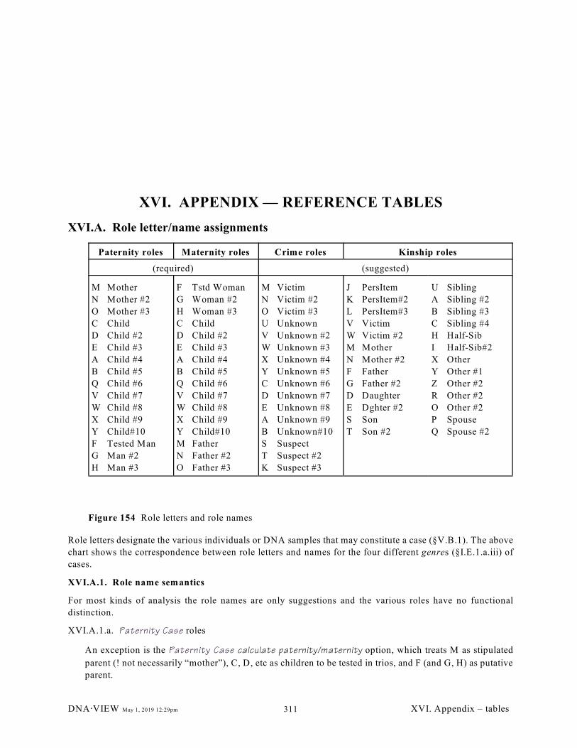
Paternity roles Maternity roles Crime roles Kinship roles
(required) (suggested)
M Mother
N Mother #2
O Mother #3
C Child
D Child #2
E Child #3
A Child #4
B Child #5
Q Child #6
V Child #7
W Child #8
X Child #9
Y Child#10
F Tested Man
G Man #2
H Man #3
F Tstd Woman
G Woman #2
H Woman #3
C Child
D Child #2
E Child #3
A Child #4
B Child #5
Q Child #6
V Child #7
W Child #8
X Child #9
Y Child#10
M Father
N Father #2
O Father #3
M Victim
N Victim #2
O Victim #3
U Unknown
V Unknown #2
W Unknown #3
X Unknown #4
Y Unknown #5
C Unknown #6
D Unknown #7
E Unknown #8
A Unknown #9
B Unknown#10
S Suspect
T Suspect #2
K Suspect #3
J PersItem
K PersItem#2
L PersItem#3
V Victim
W Victim #2
M Mother
N Mother #2
F Father
G Father #2
D Daughter
E Dghter #2
S Son
T Son #2
U Sibling
A Sibling #2
B Sibling #3
C Sibling #4
H Half-Sib
I Half-Sib#2
X Other
Y Other #1
Z Other #2
R Other #2
O Other #2
P Spouse
Q Spouse #2
Figure 154 Role letters and role names
XVI. APPENDIX — REFERENCE TABLES
XVI.A. Role letter/name assignments
Role letters designate the various individuals or DNA samples that may constitute a case (§V.B.1). The above
chart shows the correspondence between role letters and names for the four different genres (§I.E.1.a.iii) of
cases.
XVI.A.1. Role name semantics
For most kinds of analysis the role names are only suggestions and the various roles have no functional
distinction.
XVI.A.1.a. Paternity Case roles
An exception is the Paternity Case calculate paternity/maternity option, which treats M as stipulated
parent (! not necessarily “mother”), C, D, etc as children to be tested in trios, and F (and G, H) as putative
parent.
DNA@VIEW May 1, 2019 12:29pm XVI. Appendix – tables311
XVI.A.1.b. Screen disaster matches and personal references
For purposes of mass victim identification – Screen disaster matches , it can be advantageous (see
§VII.B.1.a.ii) to designate personal items with the role letters J, K, and L, per Figure 154.
But otherwise – in a Kinship or Crime (mixed-stain) context, a person is a Sibling or a Suspect not because of
the role letter, but because of the way the letter is used. However –
XVI.A.1.c. Automatically generated kinship scenario
DNA @VIEW can automatically generate a kinship scenario if you use role letters according the the
suggestion for Kinship in the role letter table in §XVI.A. This applies to
XVI.A.1.c.i.) The scenario-entry facility described in §VI.F.1.b.i;
XVI.A.1.c.ii.) and optionally can be accessed in Disaster screening if you use pedigree searching
(experimental facility – documentation pending).
XVI.A.1.d. Custom names
There is no user-friendly interface to re-define the role names, but a new set of names can be provided for
free on request.
DNA@VIEW May 1, 2019 12:29pm XVI. Appendix – tables312
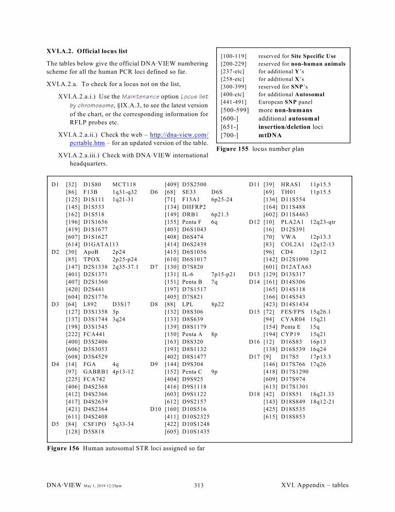
[100-119] reserved for Site Specific Use
[200-229] reserved for non-human animals
[237-etc] for additional Y’s
[258-etc] for additional X’s
[300-399] reserved for SNP’s
[400-etc] for additional Autosomal
[441-491] European SNP panel
[500-599] more non-humans
[600-] additional autosomal
[651-] insertion/deletion loci
[700-] mtDNA
Figure 155 locus number plan
D1 [32] D1S80 MCT118
[86] F13B 1q31-q32
[125] D1S111 1q21-31
[145] D1S533
[162] D1S518
[196] D1S1656
[419] D1S1677
[607] D1S1627
[614] D1GATA113
D2 [30] ApoB 2p24
[85] TPOX 2p25-p24
[147] D2S1338 2q35-37.1
[401] D2S1371
[407] D2S1360
[420] D2S441
[604] D2S1776
D3 [64] L892 D3S17
[127] D3S1358 3p
[137] D3S1744 3q24
[198] D3S1545
[222] FCA441
[400] D3S2406
[606] D3S3053
[608] D3S4529
D4 [14] FGA 4q
[97] GABRB1 4p13-12
[225] FCA742
[406] D4S2368
[412] D4S2366
[417] D4S2639
[421] D4S2364
[611] D4S2408
D5 [84] CSF1PO 5q33-34
[128] D5S818
[409] D5S2500
D6 [68] SE33 D6S
[71] F13A1 6p25-24
[134] DHFRP2
[149] DRB1 6p21.3
[155] Penta F 6q
[403] D6S1043
[408] D6S474
[414] D6S2439
[415] D6S1056
[610] D6S1017
D7 [130] D7S820
[131] IL-6 7p15-p21
[151] Penta B 7q
[197] D7S1517
[405] D7S821
D8 [88] LPL 8p22
[132] D8S306
[133] D8S639
[139] D8S1179
[150] Penta A 8p
[163] D8S320
[193] D8S1132
[402] D8S1477
D9 [144] D9S304
[152] Penta C 9p
[404] D9S925
[416] D9S1118
[603] D9S1122
[612] D9S2157
D10 [160] D10S516
[411] D10S2325
[422] D10S1248
[605] D10S1435
D11 [39] HRAS1 11p15.5
[69] TH01 11p15.5
[136] D11S554
[164] D11S488
[602] D11S4463
D12 [10] PLA2A1 12q23-qtr
[16] D12S391
[70] VWA 12p13.3
[83] COL2A1 12q12-13
[96] CD4 12p12
[142] D12S1090
[601] D12ATA63
D13 [129] D13S317
D14 [161] D14S306
[165] D14S118
[166] D14S543
[423] D14S1434
D15 [72] FES/FPS 15q26.1
[94] CYAR04 15q21
[154] Penta E 15q
[194] CYP19 15q21
D16 [12] D16S83 16p13
[138] D16S539 16q24
D17 [9] D17S5 17p13.3
[146] D17S766 17q26
[418] D17S1290
[609] D17S974
[613] D17S1301
D18 [42] D18S51 18q21.33
[143] D18S849 18q12-21
[425] D18S535
[615] D18S853
Figure 156 Human autosomal STR loci assigned so far
XVI.A.2. Official locus list
The tables below give the official DNAAVIEW numbering
scheme for all the human PCR loci defined so far.
XVI.A.2.a. To check for a locus not on the list,
XVI.A.2.a.i.) Use the Maintenance option Locus list
by chromosome, §IX.A.3, to see the latest version
of the chart, or the corresponding information for
RFLP probes etc.
XVI.A.2.a.ii.) Check the web – http://dna-view.com/
pcrtable.htm – for an updated version of the table.
XVI.A.2.a.iii.) Check with DNAAVIEW international
headquarters.
DNA@VIEW May 1, 2019 12:29pm XVI. Appendix – tables313

D19 [76] D19S253 19p13.1
[140] MYD 19q13.3
[148] D19S433 19q12-13.
D20 [92] D20S161
[135] D20S470
[199] D20S156
[413] D20S480
[600] D20S1082
[616] D20S482
D21 [99] D21S11
[153] Penta D 21q
[410] D21S2055
D22 [156] Penta G 22q
[159] D22S684
[424] D22S1045
Figure 157 more human autosomal STR loci assigned so far
STR loci – sex-linked
DX [18] DXS52
[89] HPRTB DXq26.1
[90] Amelogeni
[250] DXS101
[251] DXS10011
[252] DXS8378 Xp22
[253] DXS9895
[254] DXS9898
[255] DXS8377
[256] DXS7424
[257] GATA172D5
[258] DXS10135 Xp22.31
[259] DXS10101 Xq26.3
[260] DXS7132 Xq11.2
[261] DXS10074 Xq28
[262] DXS10134 Xq11
[263] DXS7423 Xq28
[264] DXS6800
[265] HumARA
[266] DXS6789
[267] GATA31E08
[268] DXS7133
[269] GATA165B12
[270] DXS6809
[271] DXS10075
[272] DXS10079 Xp11
[273] DXS6807
[274] DXS10148 Xp22
[275] DXS10103 Xq26.2
[276] DXS10146 Xq28
DY [167] DYS19
[168] DYS389I
[169] DYS389II
[170] DYS390
[171] DYS391
[172] DYS392
[173] DYS393
[174] DYS385a
[175] DYCAIIa
[176] DYS437
[177] DYS438
[178] DYS439
[179] DYS388
[180] DYS434
[181] DYS435
[182] DYS436
[183] DY-A4
[184] DYS460
[185] DYS461
[186] DY-A8
[187] DY-A10
[188] DYS635
[189] YGATAH4
[190] DYS426
[191] DYS447
[192] DYS448
[230] DYS464
[231] DYS446
[232] DYS463
[233] DYS458
[234] DYS456
[235] DYS452
[236] DYS449
[237] DYS385b
[238] DYCAIIb
Figure 158 Human sex-linked PCR loci assigned so far
D4 [123] GYPA
[124] Gc 4q12-13
D6 [41] DQAI 6p21.3
[195] HLADRB
D7 [122] D7S8
D11 [120] HBGG 11p15.5
D19 [121] LDLR 19p13
Figure 159 Polymarker locus
assignments
DNA@VIEW May 1, 2019 12:29pm XVI. Appendix – tables314
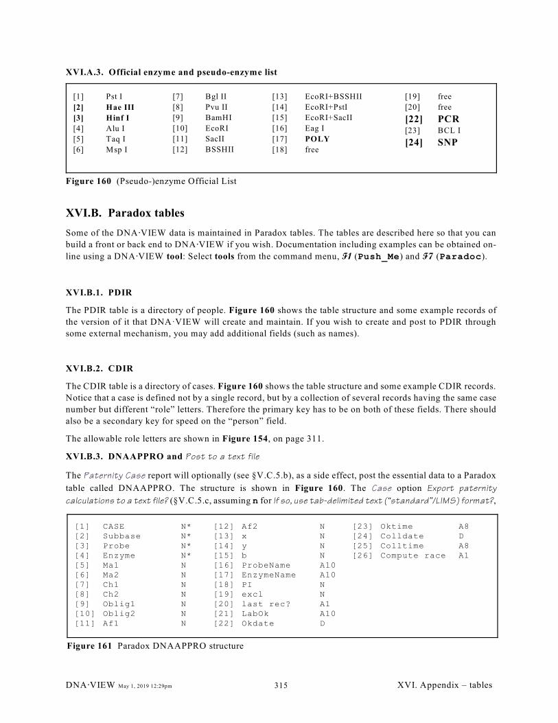
[1] Pst I
[2] Hae III
[3] Hinf I
[4] Alu I
[5] Taq I
[6] Msp I
[7] Bgl II
[8] Pvu II
[9] BamHI
[10] EcoRI
[11] SacII
[12] BSSHII
[13] EcoRI+BSSHII
[14] EcoRI+PstI
[15] EcoRI+SacII
[16] Eag I
[17] POLY
[18] free
[19] free
[20] free
[22] PCR[23] BCL I
[24] SNP
Figure 160 (Pseudo-)enzyme Official List
[1] CASE N*[2] Subbase N*[3] Probe N*[4] Enzyme N*[5] Ma1 N[6] Ma2 N[7] Ch1 N[8] Ch2 N[9] Oblig1 N[10] Oblig2 N[11] Af1 N
[12] Af2 N[13] x N[14] y N[15] b N[16] ProbeName A10[17] EnzymeName A10[18] PI N[19] excl N[20] last rec? A1[21] LabOk A10[22] Okdate D
[23] Oktime A8[24] Colldate D[25] Colltime A8[26] Compute race A1
Figure 161 Paradox DNAAPPRO structure
XVI.A.3. Official enzyme and pseudo-enzyme list
XVI.B. Paradox tables
Some of the DNA@VIEW data is maintained in Paradox tables. The tables are described here so that you can
build a front or back end to DNA@VIEW if you wish. Documentation including examples can be obtained on-
line using a DNA@VIEW tool: Select tools from the command menu, F1 (Push_Me) and F7 (Paradoc).
XVI.B.1. PDIR
The PDIR table is a directory of people. Figure 160 shows the table structure and some example records of
the version of it that DNA·VIEW will create and maintain. If you wish to create and post to PDIR through
some external mechanism, you may add additional fields (such as names).
XVI.B.2. CDIR
The CDIR table is a directory of cases. Figure 160 shows the table structure and some example CDIR records.
Notice that a case is defined not by a single record, but by a collection of several records having the same case
number but different “role” letters. Therefore the primary key has to be on both of these fields. There should
also be a secondary key for speed on the “person” field.
The allowable role letters are shown in Figure 154, on page 311.
XVI.B.3. DNAAPPRO and Post to a text file
The Paternity Case report will optionally (see §V.C.5.b), as a side effect, post the essential data to a Paradox
table called DNAAPPRO. The structure is shown in Figure 160. The Case option Export paternity
calculations to a text file? (§V.C.5.c, assuming n for If so, use tab-delimited text (“standard”/LIMS) format?,
DNA@VIEW May 1, 2019 12:29pm XVI. Appendix – tables315
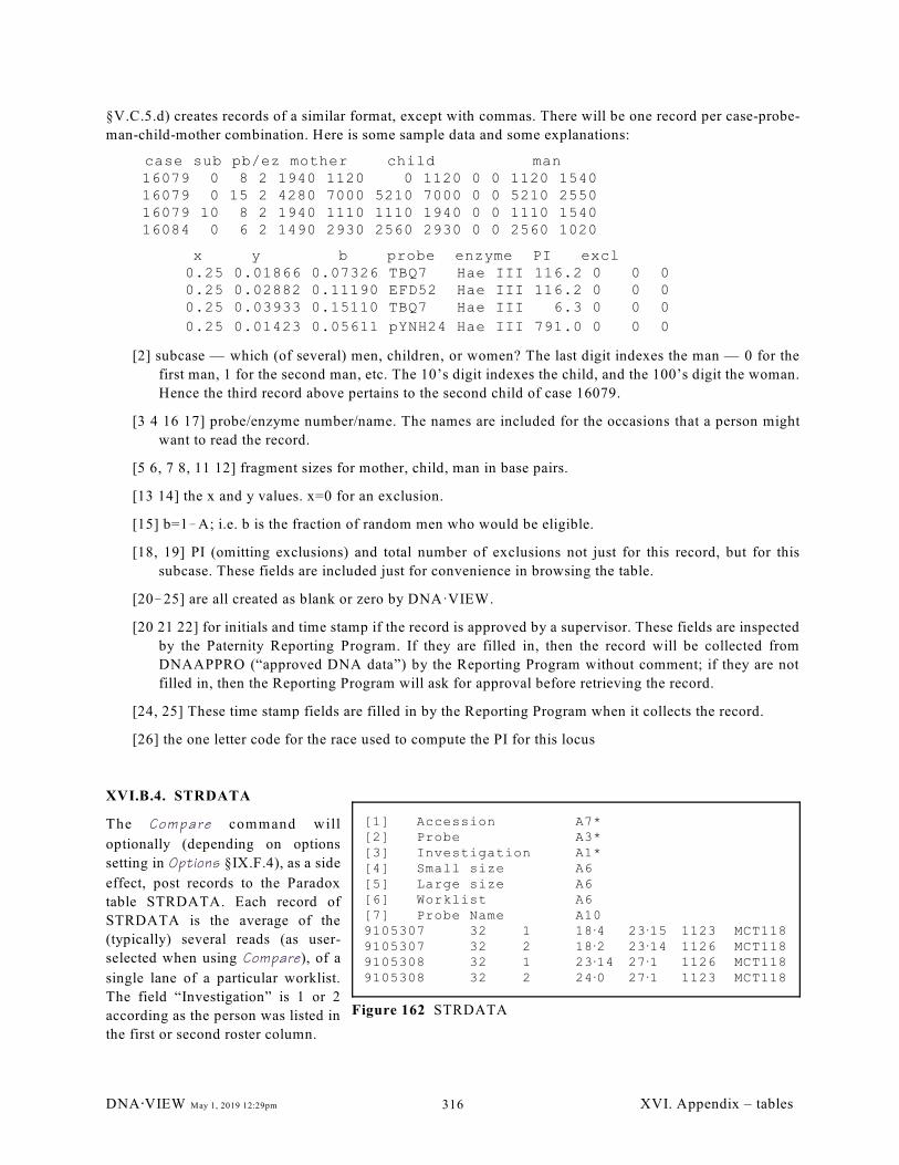
[1] Accession A7*[2] Probe A3*[3] Investigation A1*[4] Small size A6[5] Large size A6[6] Worklist A6[7] Probe Name A109105307 32 1 18A4 23A15 1123 MCT1189105307 32 2 18A2 23A14 1126 MCT1189105308 32 1 23A14 27A1 1126 MCT1189105308 32 2 24A0 27A1 1123 MCT118
Figure 162 STRDATA
§V.C.5.d) creates records of a similar format, except with commas. There will be one record per case-probe-
man-child-mother combination. Here is some sample data and some explanations:
case sub pb/ez mother child man 16079 0 8 2 1940 1120 0 1120 0 0 1120 1540 16079 0 15 2 4280 7000 5210 7000 0 0 5210 2550 16079 10 8 2 1940 1110 1110 1940 0 0 1110 1540 16084 0 6 2 1490 2930 2560 2930 0 0 2560 1020
x y b probe enzyme PI excl0.25 0.01866 0.07326 TBQ7 Hae III 116.2 0 0 00.25 0.02882 0.11190 EFD52 Hae III 116.2 0 0 00.25 0.03933 0.15110 TBQ7 Hae III 6.3 0 0 0
0.25 0.01423 0.05611 pYNH24 Hae III 791.0 0 0 0
[2] subcase — which (of several) men, children, or women? The last digit indexes the man — 0 for the
first man, 1 for the second man, etc. The 10’s digit indexes the child, and the 100’s digit the woman.
Hence the third record above pertains to the second child of case 16079.
[3 4 16 17] probe/enzyme number/name. The names are included for the occasions that a person might
want to read the record.
[5 6, 7 8, 11 12] fragment sizes for mother, child, man in base pairs.
[13 14] the x and y values. x=0 for an exclusion.
[15] b=1!A; i.e. b is the fraction of random men who would be eligible.
[18, 19] PI (omitting exclusions) and total number of exclusions not just for this record, but for this
subcase. These fields are included just for convenience in browsing the table.
[20!25] are all created as blank or zero by DNA·VIEW.
[20 21 22] for initials and time stamp if the record is approved by a supervisor. These fields are inspected
by the Paternity Reporting Program. If they are filled in, then the record will be collected from
DNAAPPRO (“approved DNA data”) by the Reporting Program without comment; if they are not
filled in, then the Reporting Program will ask for approval before retrieving the record.
[24, 25] These time stamp fields are filled in by the Reporting Program when it collects the record.
[26] the one letter code for the race used to compute the PI for this locus
XVI.B.4. STRDATA
The Com pare command will
optionally (depending on options
setting in Options §IX.F.4), as a side
effect, post records to the Paradox
table STRDATA. Each record of
STRDATA is the average of the
(typically) several reads (as user-
selected when using Compare), of a
single lane of a particular worklist.
The field “Investigation” is 1 or 2
according as the person was listed in
the first or second roster column.
DNA@VIEW May 1, 2019 12:29pm XVI. Appendix – tables316
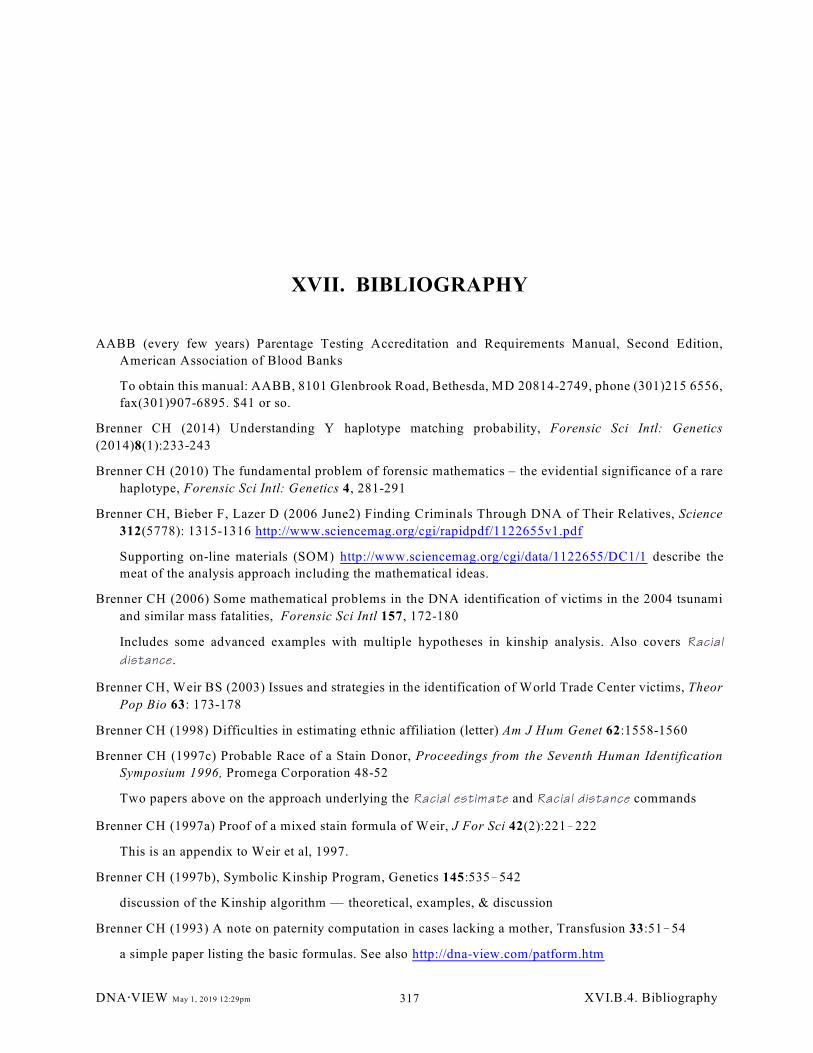
XVII. BIBLIOGRAPHY
AABB (every few years) Parentage Testing Accreditation and Requirements Manual, Second Edition,
American Association of Blood Banks
To obtain this manual: AABB, 8101 Glenbrook Road, Bethesda, MD 20814-2749, phone (301)215 6556,
fax(301)907-6895. $41 or so.
Brenner CH (2014) Understanding Y haplotype matching probability, Forensic Sci Intl: Genetics
(2014)8(1):233-243
Brenner CH (2010) The fundamental problem of forensic mathematics – the evidential significance of a rare
haplotype, Forensic Sci Intl: Genetics 4, 281-291
Brenner CH, Bieber F, Lazer D (2006 June2) Finding Criminals Through DNA of Their Relatives, Science
312(5778): 1315-1316 http://www.sciencemag.org/cgi/rapidpdf/1122655v1.pdf
Supporting on-line materials (SOM) http://www.sciencemag.org/cgi/data/1122655/DC1/1 describe the
meat of the analysis approach including the mathematical ideas.
Brenner CH (2006) Some mathematical problems in the DNA identification of victims in the 2004 tsunami
and similar mass fatalities, Forensic Sci Intl 157, 172-180
Includes some advanced examples with multiple hypotheses in kinship analysis. Also covers Racial
distance.
Brenner CH, Weir BS (2003) Issues and strategies in the identification of World Trade Center victims, Theor
Pop Bio 63: 173-178
Brenner CH (1998) Difficulties in estimating ethnic affiliation (letter) Am J Hum Genet 62:1558-1560
Brenner CH (1997c) Probable Race of a Stain Donor, Proceedings from the Seventh Human Identification
Symposium 1996, Promega Corporation 48-52
Two papers above on the approach underlying the Racial estimate and Racial distance commands
Brenner CH (1997a) Proof of a mixed stain formula of Weir, J For Sci 42(2):221!222
This is an appendix to Weir et al, 1997.
Brenner CH (1997b), Symbolic Kinship Program, Genetics 145:535!542
discussion of the Kinship algorithm — theoretical, examples, & discussion
Brenner CH (1993) A note on paternity computation in cases lacking a mother, Transfusion 33:51!54
a simple paper listing the basic formulas. See also http://dna-view.com/patform.htm
DNA@VIEW May 1, 2019 12:29pm XVI.B.4. Bibliography317
Buckleton J, Triggs CM, Walsh SJ (2005) Forensic DNA Evidence Interpretation, CRC Press
Butler JM (2005) Forensic DNA Typing – Biology, Technology, and Genetics of STR Markers, 2 edition,nd
Elsevier Academic Press
Curran JM, Triggs CM, Buckleton J, Weir B.S. (1999) Interpreting DNA mixtures in structured populations.
J Forensic Sci 44(5):987–995
a carefully written paper with an elegant result for incorporating è in a mixture calculation
Dawid AP & Mortera J (1996) Coherent Analysis of Forensic Identification Evidence, J. R. Statist. Soc. B 58,
No. 2, 425!443
Among other things this paper discusses (in section 8.3) how the databases can themselves be regarded
as data. For a discussion start at http://dna-view.com/CoherentAnalysis.htm.
Essen-Möller E, (1938) Beweiskraft der Ähnlichkeit im Vaterschaftsnachweis — Theoretische Grundlagen.
Mitt Anthrop Ges (Wien) 68:9!53. (Mitteilungen der Anthropologischen Gesellschaft; The evidential
value of similarity as proof of paternity, fundamental principles.)
introducing the likelihood ratio (in the form Y/X) for paternity
Essen-Möller E, Quensel CE (1939) Zur Theorie des Vaterschaftsnachweises auf Grund von Ähnlichkeits-
befunden. Dtsch Z Ges Gerichtl Med 31:70!96. Deutsche Zeitschrift für Gesamte Gerichtliche Medizin
famous early paper which introduced the idea of using Bayes’ Theorem for understanding paternity
evidence, but failed to understand the role of prior probabilities. They seemed to think that the scientist
could be neutral by choosing a 50% prior (as opposed to no prior at all as we understand nowadays).
Evett I et al (1990) Bayesian Analysis of Single Locus DNA Profiles, Data Acquisition and Statistical Analysis
for DNA Typing Laboratories in Proceedings for the International Symposium on Human Identification,
Promega Corporation 1990
advocates a non-matching paradigm for DNA profile analysis. Comparable to the method of Gjertson for
paternity, but presented in a much less technical fashion.
Ewens WJ (1972) The Sampling Theory of Selectively Neutral Alleles, Theor.Pop.Bio 3:87!112
a famous paper whose simple consequence is often overlooked: There figures to be an almost
inexhaustible supply of rare alleles.
Fimmers R, Schneider PM, Baur MP (1991) Comparison of Different Methods for the Calculation of Indices
of Paternity in Advances in Forensic Haemogenetics 4, Eds C.Rittner & P.M.Schneider, pp 277!284,
Springer-Verlag Berlin
Gill P, Brenner CH, Buckleton JS, et al. (2006) DNA commission of the International Society of Forensic
Genetics: Recommendations on the interpretation of mixtures, Forensic Sci Intl , 160 (2-3), 90-101
http://www.isfg.org/public.htm
Guo & Thompson (1992) Performing the Exact Test of Hardy-Weinberg Proportion for Multiple Alleles,
Biometrics 48:361!372
seminal paper leading the way to showing how Fischer’s exact test (§VIII.G) idea comes of age in the
computer era.
Morris JW, Garber RA, D’Autremont J, Brenner C (1988) The Avuncular Index and the Incest Index,
Advances in Forensic Haemogenetics 2:607!611, Springer-Verlag
when the putative father is eliminated, we compute an “avuncular index” (§V.B.4.d) for the chance that
his un-tested brother may be the father
DNA@VIEW May 1, 2019 12:29pm XVI.B.4. Bibliography318
Puch-Solis R et al (2013) Evaluating forensic DNA profiles using peak heights, allowing for multiple donors,
allelic dropout and stutters, Forensic Sci Intl: Genetics (2013)7(5):555-563
Weir BS, Triggs CM, Starling L, Stowell LI, Walsh KAJ, Buckleton J. (1997) Interpreting DNA mixtures. J
For Sci 42(2)213!222
a clear and standard exposition of the combinatorial formulas for evaluating mixed stains
Weir BS (1996) Genetic Data Analysis, Sinauer Associates, Inc.
Weir BS, Evett IW (1998) Interpreting DNA Evidence, Sinauer Associates, Inc.
Zaykin, Shivotovsky, Weir (1995) Exact test for association between alleles at arbitrary numbers of loci,
Genetica 96:169!178
generalizes Guo & Thompson to the analysis of one or several loci
DNA@VIEW May 1, 2019 12:29pm XVI.B.4. Bibliography319
Index
1-banded pattern 273
1-letter probe codes 54
3-banded patterns 167
AABB accreditation
ARM (manual) 317
homozygosity statistic 170
PI formulas 278
ABI data import
Genotyper 231, 232
Abort
editing with ctrl-q 294
from delay 21
kinship computation 137
special editing screen 294
Accession number
and Norman Conquest 230
directory 219
editing 50
entry 292
lookup by case 293
of homozygotes 168
scheme 22
Add allele to database
<Case> option 59
Add role
to <paternity/kinship/crime case> 43
Algorithm
determine ä 275
mutation 280
paternity index 278
Allele probability
Case Options 59
Allele report 187
Alleles
type in 39
Allelic dropout
and kinship 155
Amelogenin
define notation 205
Amusement
algebraic simplification 137
pause <Screen disaster matches> 149
random DNA profile 85
random subpopulation 183
Analyze database statistics 170
Answers
wrong 253
ASCII
and symbol sets 213
Assailants
multiple 76
Assign race to worklist 156
Automatic kinship 109
estimate relationships 117
report 113
report file 63
show genotypes 121
simulations 124
tutorial 37
twins 141
Avuncular index
calculate avuncular 45
generalized (trio/duo) 45
Backup
to tape 255
via network 255
Batch analysis of cases 44
Bayes' Theorem 261, 262
"non-Bayesian" 262
Bibliography 317
Brenner & Morris 172
Brenner, "Motherless" 317
Brenner, ethnic affiliation 317
Brenner, Kinship 317
Brenner, Probable race 317
Essen-Möller & Quensel 264, 318
Evett et al, "Bayesian Analysis" 318
Ewens 318
Guo & Thompson 179, 318
Bins
floating 276, 278
Browse 209
change name or comment 209
lane deletion 209
read deletion 210
worklist, etc. deletion 210
Burn victim 142
Calculate report
paternity/crime case option 47
Cap on PI 60
Cascade of deletions 210
Case 22
<open case> 41
<paternity/kinship/crime case> 41
add or edit comment 50
ambiguous 94
automatic mixture 65
deficiency 99
DNA@VIEW May 1, 2019 12:29pm Index320
define 56
definition 41
edit case comment 50
export 51
extra person 43
find comment 57
find worklists 93
incest 99
numbers 22, 293
parameters 234
popular 56
summary report 54
with no mother 278
Case comment
edit 50
find 57
import 234
type and races 234
Case number
format 211
select 56
Case options 58
add allele to database 59
ask before posting 61
include empirical PI 64
include QC 63
minimum frequency calculation 60
minimum Gjertson PI 64
motherless if exclusion 59, 283
mutations allowed 60
NML method 64
post consensus 63
post to text file 61, 63, 315
Stat Sheet 63
use Gjertson PI 64
Cases
list 52
Casework menu 41
CGI.CFG 300
Change
database name 167
worklist date 209
Character translation 213
Children
in Tibet 269
multiple 43
Choices 287
multiple 288
Co-electrophoresis
lane notation 208
resolution 267
CODIS
create CMF file 250
define QC values 221
Color printer
plotting 173
Colors
modify <Plot> 172
Combine
databases 167
Command
menu style 212
Compare report 219
options 212
CompareSwitch 199
Compute one locus 49
CONFIG.APL
wssize 301
CONFIG.NT 301
Consensus 63
Consultation
Kinship case 123
Convicted offender
database 162
database search 162, 249
Copy and paste 290
from Windows 290
Count
rare alleles 59, 60
Create
worklist 93
Crime case
analysis 76
logic 76
roles 75
Y-haplotype 87
Data
backing up 255
Data entry
dates 291
numbers 290
people 292
text 290
yes-no 291
Database
<Analyze database statistics> 170
command 158
compile 165
exception report 166
printout 169
rebuild defaults 166
rename 167
DNA@VIEW May 1, 2019 12:29pm Index321
set default 160
type in 168
updating 166
Database similarity test 186
Databases
3-banded patterns 167
build & maintain 162
combine 167
convicted offender 249
create or compile 158
edit manually 168
export 247
find duplicates 245, 248
import 246
install additional 301
missing person 249
search profiles 247
set default 160
statistics 170
storage of 254
swap between users 246
updating 167
Date order 212
Decimal marker 212
Default database 159
specify 160
specify on-the-fly 49
updating 166
Delete
case 50
configuration 210
database 167
lane 209
person from case 44
read 93, 210
standards ladder 210
worklist 93, 210
Delta
<PI> parameter 267
algorithm to determine 275
Demonstration system 256
Did you know? 303
Directory 219
Disaster
screening 148
test candidates 153
Discussion
1-banded patterns 273
Allele count 59, 60
Bayes' Theorem 261
independence failure 184
multiple assailants 76
mutation 284
paternity index 268
Divisors
in co-electrophoresis PI 267
DNA calculations
export format 315
DNA data
proofread 120
DNA Exclusion 89
null allele 89
DNA Odds 84
DNA Profiles
command 97
DNAAPPRO
format of 315
DNA·VIEW
moving 307
User's group; database sharing 246
Dropout calculation
in <Kinship> 122
pairwise relationships 116
Dropout tolerance
in <Worklist collapse> 146, 147
Edit a database 168
Edit case comment 50
Empirical PI 64
Enzyme
and pseudo-enzyme, official list 315
assign to locus 204
restriction 207
STR as pseudo- 40
Errors
file compression 200
FILE DATA ERROR 258
file handles 301
host access 304
in answers 253
program 253
reporting 253
Essen-Möller
equation 264
Exact test 178
database similarity (Fisher/Brenner) 186
Hardy-Weinberg equilibrium 179
Exclusion
<DNA Exclusion> command 89
# loci needed 281
definition 89
expected rates 180
false (mutations) 205
DNA@VIEW May 1, 2019 12:29pm Index322
indirect 142
limitations 89
maternal 59, 283
mixed stain model 71
probability in paternity 269
probability, formula 89
Exclusion probability
formula (mixed stain) 89
Exit DNAAVIEW 21
Experimental features 172
Export
databases 247
DNA calculations 315
simulated case 127
Export case 51
simulated 127
Extra people
crime case 75
in <paternity/kinship/crime case> 43
Family case
calculate 49
Far out 220
Fax
assistance 20
FILE DATA ERROR 258
File handles
Windows XP/2000/NT 301
file locking 306
File menu 96
FileCompress
prevents file rot 258
Files
of DNAAVIEW 254
Find
matching profiles 247
Fix
network lock 259, 260
Fly, on the
add or change reader 198
specify default database 49
Flying window key 304
Forensic case 65
Formula
Bayes 106
Essen-Möller 264
exclusion (mixture) 89
exclusion probability (mixed stain) 89
matching LR 76
matching odds 76
motherless case 278
multiple assailant 76
mutation model 284
paternity index 268
W 263, 268
Frequency
Case Options 59
computation 275
of rare alleles 59, 60
of rare alleles, <Screening> 205
Friday backup 255
GeneMapper import 226, 231
underscore as space 236
Genetic type 40
Genotyper import 226
Genotypes
proofread 120
Gjertson model
set minimum PI 64
use as standard 64
Good part
default database 161
Graphics
scaling of details 214
Half sibling 99
Hardware 17
Hardy-Weinberg equilibrium
test for 179, 183
Help
telephone or fax 20
Hitachi STRCall import 232
Homozygosity
inconsistent 166
vs. single-bandedness 279
Homozygotes
<Plot> option 172
records kept 166
Host Access Error 304
Hypotheses
<Kinship> 106
Icon
customize 300
start, maintenance 298
Immigration
/kinship 110
vs. <Kinship> 100
Import
populaton database 240
Import wizard
Genemapper 226, 227, 231
Genotyper 226, 230
Hitachi STRCALL 232
Import/export
DNA@VIEW May 1, 2019 12:29pm Index323
case import 250
cases 250
CODIS export 250
create phenotype list 247
export database 247
find duplicates 247
GeneMapper data 226, 231
Genotyper data 226
import database 243, 246
Incest 99
experiment 126
Independence
exact test 178
test for 179, 183
Index 320
avuncular 45
paternity 263
Installation 2
databases 301
DNAAVIEW 295
quick 33
retreat from 300
test platform 308
write-back caching 306
Interassay
standard deviation 222
Internet
email 2
upgrades 2
web site 2
Interpolation method
choose parameters 214
Intraassay statistics 208
Key
hardware security 303
Keyboard
national language 214
use of 287
Kinship 25
"parsing" option 120
"parsing" toggle 136
è 122
automatic version 109, 110
candidate 148
estimate relationships 116
hypotheses 106
in mixture case, limitation 75
long scenarios 112
missing person problem 142
modify problem 134
null alleles 105
option toggles 135
semantics 105
show pairwise relationships 117
simple way 104
simulation 124
stand-alone version 133, 134
Symbolic Kinship Program 99
syntax rules 101
theta 122
three scenarios 271
twin problem 141
two versions 100
vs. immigration 100
Lane
definition 23
deletion 209
Language
crime roles 52
for prompts etc. 214
import for case 234
keyboard mapping 214
kinship roles 52
maternity roles 52
paternity roles 52
Likelihood ratio 263
<Kinship> case 269
explanation 269, 270
in DNAAVIEW 264
stain matching 76, 263
LIMS
integration with DNA@AVIEW 250
List
cases 52
people 52, 219
Loci/probes
add (example) 202
defining; tutorial 40
display style 214
independence test 179
maintenance 201, 203
multiplex ordering 40
official list 313
ordering 201
x-linked 136
Lock
network 254
Logic
stain case 76
Long scenarios 112
Luddite 3
Maintenance 195
DNA@VIEW May 1, 2019 12:29pm Index324
configurations 198
loci, probes 201
locus, screen 203
races 197
Readers 197
restriction enzymes 207
standards ladder 198
Manual data entry
tutorial 38
Matching
profiles, find 247
Matching LR 76, 263
Matching pattern 266
Maternal exclusion 59, 283
Maternity case
create 52
Menus
Casework 41
File 96
Minimum frequency calculation 60
Missing person 99, 142
database 162
database search 249
Mixed stain analysis 65
continuous model 80
Mixture
explorer 77
multiple suspects 67
Mixture calculator 65
continuous 65
limitations 75
practice examples 66
silent/null allele 71, 72
victim as suspect 67
Mode
graphics 21
Monte Carlo
HW exact test 180
independence check 179
kinship simulation 124
Motherless
calculation if mutation 59, 283
case 278
Mothers
multiple 43
Mouse 291
enable 300
Moving DNA@VIEW 307
Multiple assailants 76
Multiple race calculation 50
Multiple selection 288
Multiplex
as locus set 207
Genescan import 205
kinship simulation 124
probe parameters 205
user-defined 207
Mutation
<immigration/kinship> 122
AABB model 284
and kinship 154
and null alleles 283
and paternity 58
Case Options 59, 63
default rate 59
determine rate 189
discussion 280, 284
kinship switch 122
number allowed 60
principles 281
set rate 203-205
simulation switch 130
single-locus parameter 205
STR model 282
Mutation History 189
Name tag style 215
Network 305
compressing files 200
interlock 254
preferences or parameters 198
use for backup 255
NML
use method 64
Norman Conquest
accession numbers for 230
Notation
for alleles 205
NRC II
computation 86
Null allele
<Kinship> 105, 120, 135, 285
<Paternity case> option 54
and mixed stain 71, 72
and mutation 283
in <Paternity Case> 48, 279
in database 168, 245, 279
PI computation 279
vs. homozygosity 279
Numbering scheme
case 22
people 22
quality controls 22
DNA@VIEW May 1, 2019 12:29pm Index325
Numeric editor 294
Numlock key 215
Offender database
build & maintain 162
search 249
OFFLADDER allele
<Options> 215
treatment on <Import> 233
Open Case 41
Options 211
box drawing characters 211
case # format 211
date order 212
decimal marker 212
DNA@VIEW printer 213
for Case 58
keyboard 214
language 214
locus name style 214
name tag style 215
off-ladder policy 215
page format 216
PCR notation style 215
report title 214
Out
far 220
Pairwise relationships 116, 117
Paradox
CDIR 315
DNAPPRO 315
document table 198
PDIR 315
reindex tables 199, 257
remove lock 259, 260
set sort order 258
STRDATA 316
Parameters
locus 205
necessity for setting 31
PCR 204
report of settings 199
Passwords
create 200
for command restriction 200
software installation 295
PATER
boilerplate 217
switch to 256
Paternity
search database 249
Paternity case 41
batch run 44
null allele 54
report 47
report file 61
Paternity Index
algorithm 278
discussion 268
empirical 64
generalized (trio/duo) 45
make graph of 172
typical 170, 172
Patterns
1-banded 273
3-banded 167
PCR
define locus as 204
notation style 215
PCR parameters 40
genetic type 205
notation 205
report 195, 204
Pedigree/locus 133
Person
calculate profile frequency 86
Phenotypes
create list 247
matching 248
search for matching 248
PI 265
definition 268
maximum value 60
model for 266
motherless case 278
post to file 315
typical 172
Plot 171
modify colors 172
options 171
show ladder 173
Polymarker
designate locus as 204, 205
Popular case
retrieve 56
Population
import database 240
Posterior probability
threshold 119
Preserve state 199
<PI> report 267
database listing 169
DNA@VIEW May 1, 2019 12:29pm Index326
list of homozygotes 168
locus report 195
race names 197
reports 96
Printer
from Windows 302
port select 213
PrintFil (software) 298
specify 213
USB 298
PrintFil
software printer 298
Prior probability
in <Paternity case> 53
Probability 262
<Kinship> posterior 106
<Kinship> prior 106
<paternity> prior 53
conditional 261, 262
of discrimination 170
of exclusion 170
posterior 273
prior 262, 272
random match 97
relative, from race 117
simulation posterior 131
simulation prior 131
Probes/loci
see Loci/probes 320
Profile data
validation report 218
Push_Me 258
Quality controls
and case report 63
maintaining 220
omit from database 165
standard deviation 222
Race
of origin 117
Races
<Assign Race to Worklist> 156
default databases for 160
editing codes for 293
import for case 234
maintenance 197
print list 197
use in <Paternity Case> 50
Racial discrimination 192
Racial distances 192
Racial estimate 117
command 193
publications 317
Random subpopulation 183
Rare allele
<Screening> parameter 205
disaster screening parameter 205
frequency recommendation 59, 60
inexhaustible supply of 318
interpret illegal as 215
report 187
Ratio
likelihood 263
Read
delete 210
in hierarchy 210
Readers
database compilation 165, 167
list of 31, 197
maintenance 197
Recapitulation
report 54
Recent case
retrieve 56
RecordSwitch 199
disable 199
Reindex
Paradox tables 257
Remove
case 50
person from case 44
Rename
database 167
worklist 93
worklist, etc. 209
Repair
corrupt file 258
Paradox problems 259
Report
<Save As> 96
<Statistics> 209
exception 166, 167
family case 49
paternity case 47
title 214
Reprint 96
<Database> report 166
Restrict data
<Paternity/Crime Case> option 55
Restriction enzyme 207
Retreating
to previous version 300
Role
DNA@VIEW May 1, 2019 12:29pm Index327
<Paternity case> 48
add to <paternity/kinship/crime case> 43
and Sample Info field 235
in <Case>, defined 22
in <Kinship> case 109
letters and words 311
list of 311
omit descriptions 61
semantics of 229
use as <Kinship> name 101
Roster
tutorial 39
Save As 96
Screen disaster matches 148
Screening summary 152
Security key
installation 303
Select case number 56
Show pairwise relationships 117
Show report 96
Sibling 99
NRC II computation 86
Silent allele 135
indirect exclusion 142
Simulate kinship 124
Single-banded
list people in database 168
person in a case 279
Slow computer
speed up 303
SNP
define notation 205
designate locus as 204, 205
parameter values 204, 205
Standards ladder 23
create 198
delete 210
Start DNA@AVIEW
icons 298
Startup 2
Stat sheet 63
Statistical test
Independence 178
Statistics 208
intraassay 208
report 209
STR
designate locus as 204, 205
frequency computation 276
stutter
automatically account for 65
document setting 195
in a mixture 74
set typical % 195
treatment options 69, 73
Suspect
related to culprit 86
Switch system
to Demo 256
to PATER 256
Symbol set 213
SystemWide 199
Telephone
assistance 20
Test suites
<Kinship> examples 138, 251
mixture 76, 251
parentage 57, 251
simulation 252
Tested man
additional 43
Text input
date 293
numeric 290
special editing screen 294
Text output
of <Automatic kinship> data 63, 113
of <Paternity Case> data 61, 315
Theta
and <DNA odds> 85, 91
and <DNA Profiles> 97
and <Kinship> 122
and <Paternity case> 53
and avuncular 45
and mixture LR 69, 76
in <DNA Exclusion> 89, 91
in <DNA Odds> 85, 86
in <DNA Profiles> 97
Thickness graphic lines 217
Tools 257
CompareSwitch 199
Push_Me 258
RecordSwitch 199
Tutorial 35
<Automatic kinship case> 37
<DNA odds> 39
<Kinship> 34
casework 35
genotyper import 36
installation 33
manual entry 38
Twins
DNA@VIEW May 1, 2019 12:29pm Index328
<Kinship> case 141
Type in
<Kinship> scenario 111
Type in a database 168
Type in a Read
tutorial 39
Uniqueness estimate 86
Unobserved bands
<Kinship> calculation 142
Update command 253
files used by 256
USB printer
connect to 298
Validation 251
<immigration/kinship> 123
<Kinship> test case 138, 251
compute one locus 49
mixture examples 76, 251
parentage test examples 57, 251
simulation 252
Victim
logic 76
Waiting
cease 21
for table message 254
Web conference 309
Window
matching 267
style options 217
Windows
customize icon 300
flying-window key 304
lore 303
printing from 302
Windows 95 setup 303
Windows XP/2000/NT
CONFIG.NT 301
Worklist 92
change comment 209
compare reads of 219
compute profiles of 97
configuration 198
create 93
delete 210
find for case 93
tutorial 39
Worklist collapse 145
Worklist Sizes 208
Workstation name 307
on reports 214
World Trade Center
input conversion option 212
WS FULL message 301
wssize parameter 301
X-linked locus 136
Y Databases 175
Y haplotypes 174
database statistics 177
install database 175
matching odds 87
reorder databases 176
Y-chromosome
define locus on 205
independence of traits 179
Y-haplotype odds 87
and <Kinship> 117
and mutation 118
combine with <Kinship> 118
near matches 87
statistics 87
Year 2000
accession numbers 292
Yellow
banner 21
Zaykin, Shivotovsky, Weir 178, 319
DNA@VIEW May 1, 2019 12:29pm Index329