discriminating between stationary and nonand non- · pdf file · 2018-01-19and...

7/29/2012

1

Discriminating between stationary Discriminating between stationary

and nonand non--stationary stationary responsesresponses

in in catchment catchment water water and and nutrient nutrient

export export using wavelet analysisusing wavelet analysis

Irena F. Creed Western University

London, ON

Do we have adequate data to distinguish Do we have adequate data to distinguish

climate warming trends from climate warming trends from

naturally occurring climate oscillations? naturally occurring climate oscillations?

21-25 May 2012, Potsdam, Germany 2

7/29/2012

2

RationaleRationale

• Headwater catchment export signals contain a complex mix of

signals:

– Non-stationary (climate trends)

• deterministic responses where the statistical mean and variance

change with time, predictably and unpredictably

– Stationary (climate oscillations)

• stochastic responses where the statistical mean and variance do

not change with time

• In landscapes that are not impacted by human activities, if we

are able to discriminate climate trends from climate

oscillations, these headwater catchments could serve as

sentinels of climate change.


HypothesesHypotheses

• Non-stationary signal > stationary signal.

• Both signals are greater in catchments that have higher water

loading potential and/or with lower water storage capacity.

• Non-stationary signals are related to global warming while

stationary signals are related to global climate oscillations at

scales that range several years to several decades.


7/29/2012

3

Optimal time scale?Optimal time scale?

• Climate indices provided at

monthly intervals.

• We examined monthly, seasonal

and annual (water year) time

scales.

• Observed no to minimal non-

stationary signals in monthly and

seasonal time series (too variable).

• Chose to focus on annual time

series.

5

Analytical framework for Analytical framework for

signal detectionsignal detection


7/29/2012

4

Detecting nonDetecting non--stationary trendstationary trend


Detecting nonDetecting non--stationary trendstationary trend


7/29/2012

5

Analytical framework for Analytical framework for

signal detectionsignal detection


7/29/2012

6

The thin solid line (cone of influence),

delimits region not influenced by edge effect.

The thick solid lines show the

95% confidence level.

Morlet wavelet is a

sine wave (blue curve) multiplied by a

Gaussian envelope (red curve).

Rules for signal detection:

1. Signal must occur twice in record

2. Entire signal must be within half the

record

3. Select dominant signal

3. Establish baseline and identify

the scales (years) above baseline that

form the beak

4. Never select same scales (years) twice

7/29/2012

7

7/29/2012

8

7/29/2012

9

7/29/2012

10

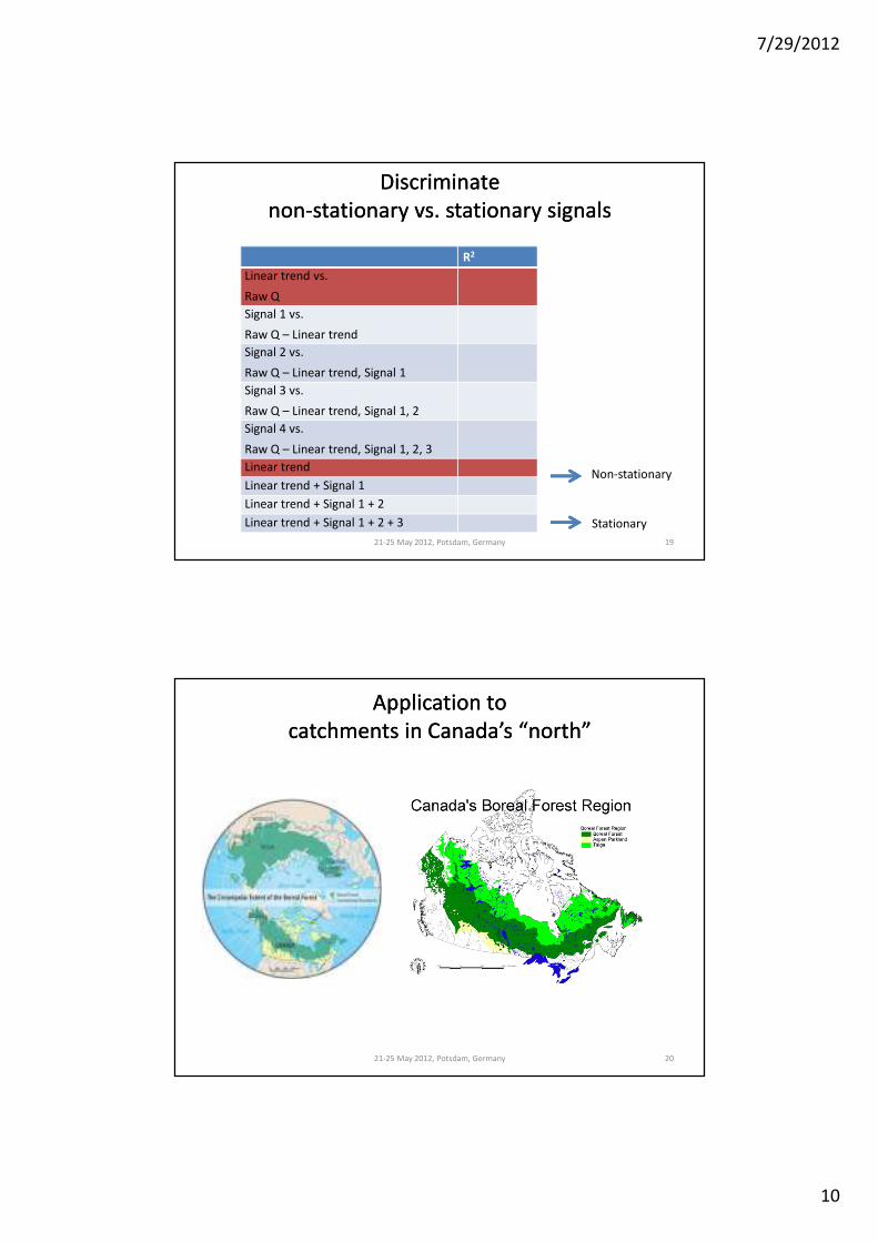
Discriminate Discriminate

nonnon--stationary vs. stationary signalsstationary vs. stationary signals

Non-stationary

Stationary

R2

Linear trend vs.

Raw Q

Signal 1 vs.

Raw Q – Linear trend

Signal 2 vs.

Raw Q – Linear trend, Signal 1

Signal 3 vs.

Raw Q – Linear trend, Signal 1, 2

Signal 4 vs.

Raw Q – Linear trend, Signal 1, 2, 3

Linear trend

Linear trend + Signal 1

Linear trend + Signal 1 + 2

Linear trend + Signal 1 + 2 + 3


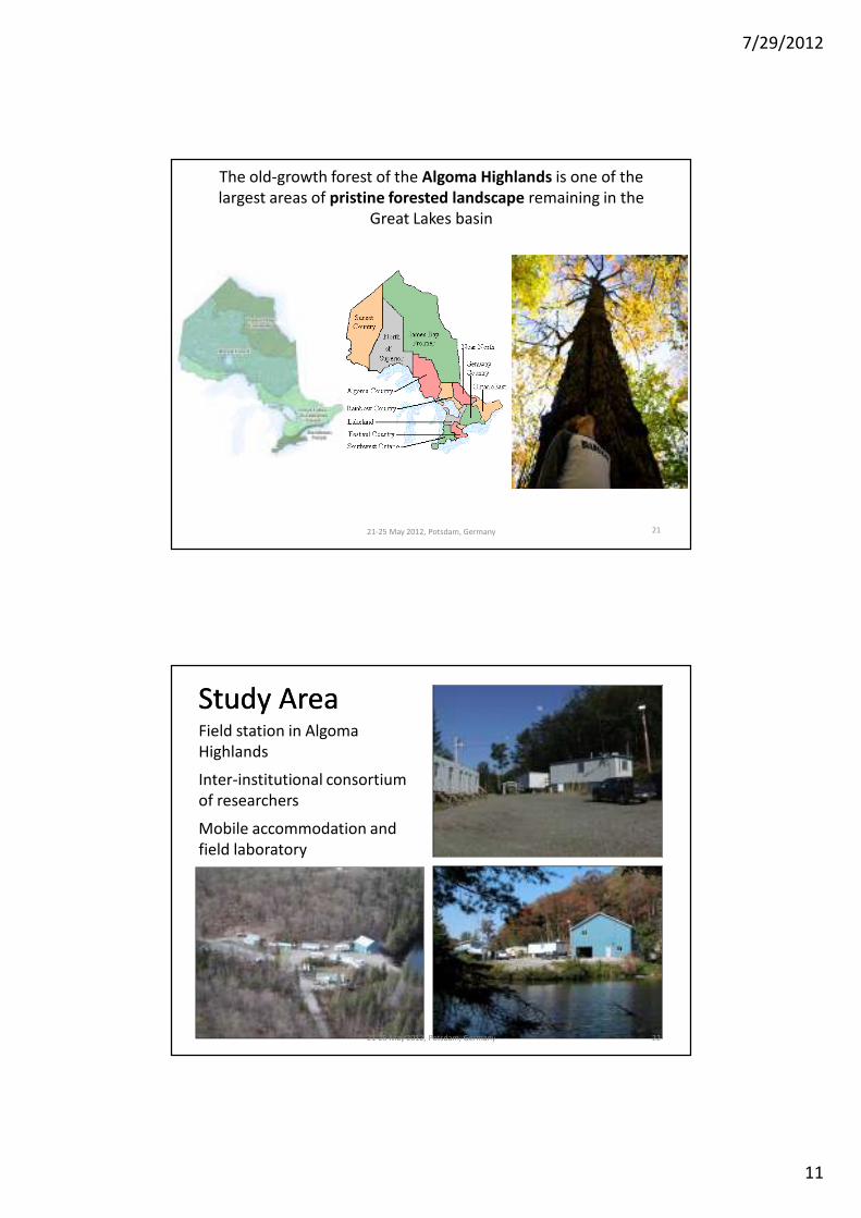
Application to Application to

catchments in Canada’s “north”catchments in Canada’s “north”


7/29/2012

11

The old-growth forest of the Algoma Highlands is one of the

largest areas of pristine forested landscape remaining in the

Great Lakes basin


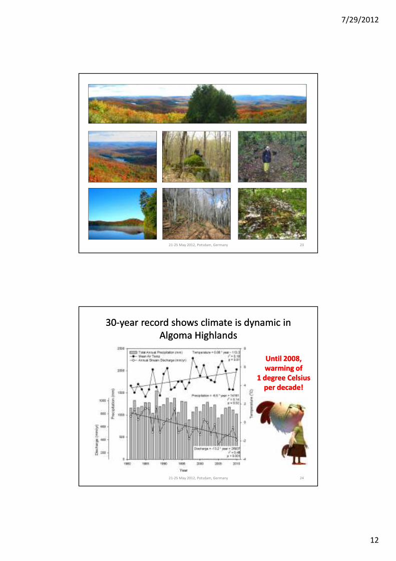
Study AreaStudy AreaField station in Algoma

Highlands

Inter-institutional consortium

of researchers

Mobile accommodation and

field laboratory


7/29/2012

12


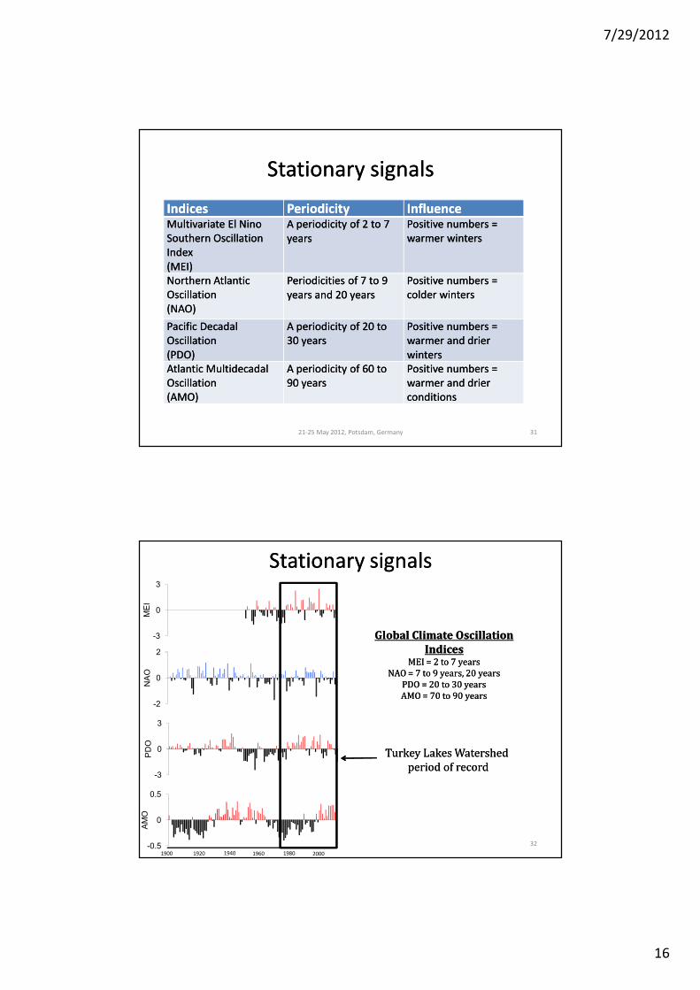
3030--year record shows climate is dynamic in year record shows climate is dynamic in

Algoma HighlandsAlgoma Highlands


Until 2008, Until 2008,

warming of warming of

1 degree Celsius 1 degree Celsius

per decade!per decade!

7/29/2012

13

c35 c38 c47 C50

Size (ha) 4.0 6.5 3.4 9.5

Water loading Lower Lower Higher Higher

Water storage (% wetland) 1 21 0.3 10

Is there similarity in catchment responsesIs there similarity in catchment responses

to climate dynamics?to climate dynamics?

25

Turkey Lakes Watershed

Since 1981, monitoring

hydrology and

biogeochemistry of 12

headwater catchments, chain

of five lakes, and Norberg

Creek that drains into Lake

Superior

Is there similarity in catchment responsesIs there similarity in catchment responses

to climate dynamics?to climate dynamics?

C35 C47

C38 C50

Higher

water loading

Hig

he

r

wa

ter

sto

rag

e


7/29/2012

14

C35

C47

C38

C50

Water Export

C35 C47

C38 C50

Higher

water loadingH

igh

er

wa

ter

sto

rag

e

Catchment water exportCatchment water export

(r(r22) )

C35C35 C38C38 C47C47 C50C50

Linear Linear trend trend vsvs..

Raw Raw QQ

0.520.52 0.440.44 NSNS 0.180.18

Linear trend (slope)Linear trend (slope) --14.814.8 --13.013.0 NSNS --8.98.9

Signal 1 vs. Signal 1 vs.

Raw Q Raw Q –– Linear Linear trendtrend

0.270.27 0.260.26 0.190.19 0.260.26


Raw Q Raw Q –– Linear trend, Signal Linear trend, Signal 1 1

0.310.31 0.260.26 0.230.23 0.280.28


Raw Q Raw Q –– Linear trend, Signal 1, Linear trend, Signal 1, 2 2

0.190.19 0.260.26 0.320.32 0.150.15


Raw Q Raw Q –– Linear trend, Signal 1, 2, 3 Linear trend, Signal 1, 2, 3

NSNS NSNS NSNS NoNo SignalSignal


7/29/2012

15

Catchment water export Catchment water export

(cumulative r(cumulative r22))

C35C35 C38C38 C47C47 C50C50

NonNon--stationary signalstationary signal 0.520.52 0.440.44 NSNS 0.180.18

Linear trend + Signal 1 Linear trend + Signal 1 0.650.65 0.590.59 0.190.19 0.390.39

Linear trend + Signal 1 + Linear trend + Signal 1 + 22 0.760.76 0.680.68 0.380.38 0.560.56

Linear trend + Signal 1 + Linear trend + Signal 1 + 2 2 + + 33 0.810.81 0.760.76 0.560.56 0.630.63

StationaryStationary signalssignals 0.290.29 0.320.32 0.560.56 0.450.45


NonNon--stationary signalsstationary signals

Climate Climate

warmingwarmingC35C35 C38C38 C47C47 C50C50

rr --0.530.53 --0.570.57 --0.370.37 --0.430.43

rr22 0.280.28 0.330.33 0.130.13 0.190.19

pp < 0.05< 0.05 < 0.05< 0.05 p=0.055p=0.055 < 0.05< 0.05


7/29/2012

16

Stationary signalsStationary signals

IndicesIndices PeriodicityPeriodicity InfluenceInfluenceMultivariate Multivariate El Nino El Nino

Southern Oscillation Southern Oscillation

Index Index

((MEI) MEI)

A periodicity of A periodicity of 2 2 to 7 to 7

yearsyears

Positive Positive numbers = numbers =

warmer warmer winterswinters

Northern Atlantic Northern Atlantic

Oscillation Oscillation

((NAO) NAO)

Periodicities of 7 Periodicities of 7 to 9 to 9

years years and and 20 years20 years

Positive numbers = Positive numbers =

colder winters colder winters

Pacific Decadal Pacific Decadal


((PDO) PDO)

A A periodicity periodicity of of 20 20 to to

30 years30 years


warmer and drier warmer and drier

winters winters

Atlantic Atlantic MultidecadalMultidecadal


((AMOAMO))

A A periodicity of 60 to periodicity of 60 to

90 years90 years


warmer and drier warmer and drier

conditionsconditions



-0.5

0

0.5

AMO

-2

0

2

NAO

-3

0

3

PDO

-3

0

3

MEI

Global Climate Global Climate OscillationOscillation

IndicesIndices

MEI MEI = 2 to 7 years= 2 to 7 years

NAO NAO = = 7 to 9 years, 20 years7 to 9 years, 20 years

PDO = PDO = 20 to 30 years20 to 30 years

AMO = AMO = 70 to 90 years70 to 90 years

Turkey Lakes Watershed Turkey Lakes Watershed

period of recordperiod of record

32

1900 1920 1940 1960 1980 2000

7/29/2012

17

Wavelet crossWavelet cross--coherence betweencoherence between

climate oscillations and water exportclimate oscillations and water exportWavelet power spectrum of MEI Index

Wavelet power spectrum of c35 water export

versus=

The thin solid line (cone of influence),

delimits region not influenced by edge effect.

The thick solid lines show the

95% confidence level.

33

Negative correlation or

precipitation lags behind NO3-

export

Positive correlation or

precipitation leads NO3- export


Wavelet crossWavelet cross--coherence betweencoherence between

climate oscillations and water exportclimate oscillations and water export

Determining Lag/Lead at a Period

phaseangle: (arrow angle * pi) / 180

Lag/Lead = phaseangle*period/(2*pi)

7/29/2012

18

-0.5

0

0.5

AMO

-2

0

2

NAO

-3

0

3

PDO

-3

0

3

MEI

Wavelet crossWavelet cross--coherence between coherence between



Higher

water loading

Hig

he

r

wa

ter

sto

rag

e

-0.5

0

0.5

AMO

-2

0

2

NAO

-3

0

3

PDO

-3

0

3

MEI

Higher

water loading

Hig

he

r

wa

ter

sto

rag

e




7/29/2012

19

-0.5

0

0.5

AMO

-2

0

2

NAO

-3

0

3

PDO

-3

0

3

MEI


Higher

water loading

Hig

he

r

wa

ter

sto

rag

e



-0.5

0

0.5

AMO

-2

0

2

NAO

-3

0

3

PDO

-3

0

3

MEI


Higher

water loading

Hig

he

r

wa

ter

sto

rag

e



Until 2008, Until 2008,

warming of warming of

1 degree Celsius 1 degree Celsius

per decade!per decade!

7/29/2012

20


MEIMEI NAONAO PDOPDO AMOAMO

MEIMEI -- 0.0110.011 0.600***0.600*** --0.1520.152

NAONAO -- -- --0.387*0.387* --0.2570.257

PDOPDO -- -- -- --0.3140.314

AMOAMO -- -- -- --

Pearson correlation matrixPearson correlation matrix


Climate oscillationsClimate oscillations C35C35 C38C38 C47C47 C50C50

MEIMEI NSNS NSNS NSNS NSNS

NAONAO NSNS NSNS NSNS NSNS

PDOPDO rr 0.380.38 -- -- --

rr22 0.150.15 -- -- --

pp < 0.05< 0.05 NSNS NSNS NSNS

AMOAMO rr --0.700.70 --0.680.68 -- --0.430.43

rr22 0.490.49 0.460.46 -- 0.190.19

pp < 0.05< 0.05 < 0.05< 0.05 NSNS < 0.05< 0.05


7/29/2012

21

AMO: Dominant global climate oscillation AMO: Dominant global climate oscillation

driving local temperature patternsdriving local temperature patterns

Findings for water exportFindings for water export


•• NonNon--stationary signal > stationary signal. stationary signal > stationary signal.

NON-STATIONARY SIGNALS GREATER IN CATCHMENTS WITH LWLP (c35, c38).

STATIONARY SIGNALS GREATER IN CATCHMENTS WITH HWLP (c47, c50).

•• Combined signals are greater in catchments that have lower water loading Combined signals are greater in catchments that have lower water loading

potential and/or with lower potential water storage capacity.potential and/or with lower potential water storage capacity.

COMBINED SIGNALS GREATEST IN CATCHMENT WITH LWLP and LWSC (c35).

•• NonNon--stationary signals are related to global warming while stationary signals stationary signals are related to global warming while stationary signals

are related to global climate oscillations at scales that range several years to are related to global climate oscillations at scales that range several years to

several decades.several decades.

SIGNFICANT RELATIONSHIPS BETWEEN CLIMATE WARMING AND CLIMATE

OSCILLATIONS AND WATER EXPORT OBSERVED.

7/29/2012

22

Should we expect the sameShould we expect the same

findings for solute export?findings for solute export?

(DOC, DON, TDP, nitrate export)(DOC, DON, TDP, nitrate export)


C35

C47

C38

C50

DOC Export

C35 C47

C38 C50

Higher

water loading

Hig

he

r

wa

ter

sto

rag

e

7/29/2012

23

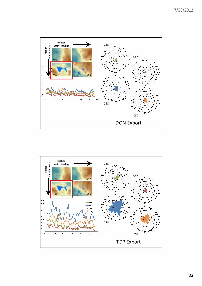
C35

C47

C38

C50

C35 C47

C38 C50

Higher

water loadingH

igh

er

wa

ter

sto

rag

e

DON Export

C35

C47

C38

C50

C35 C47

C38 C50

Higher

water loading

Hig

he

r

wa

ter

sto

rag

e

TDP Export

7/29/2012

24

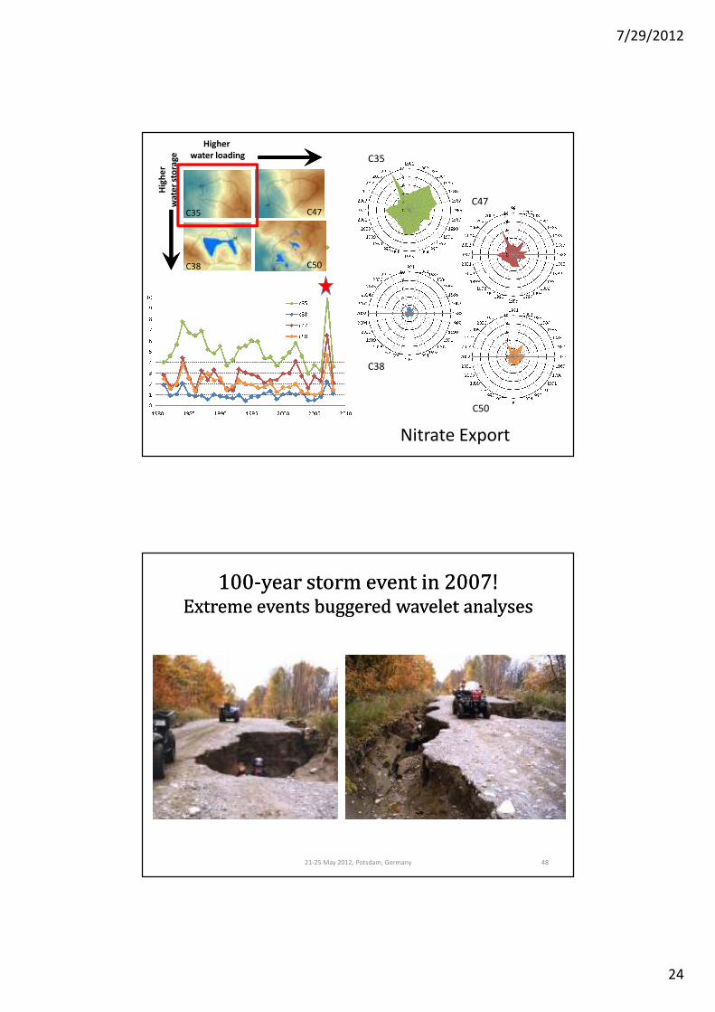
C35

C47

C38

C50

C35 C47

C38 C50

Higher

water loadingH

igh

er

wa

ter

sto

rag

e

Nitrate Export

100100--year storm event in 2007!year storm event in 2007!Extreme events buggered wavelet analysesExtreme events buggered wavelet analyses


7/29/2012

25

C35C35 C38C38 C47C47 C50C50

Non Non

StationaryStationary

StationaryStationary Non Non







WaterWater 0.520.52 0.290.29 0.440.44 0.320.32 00 0.560.56 0.180.18 0.450.45

DOCDOC 00 0.530.53 00 0.880.88 00 0.690.69 00 0.530.53

DONDON 0.800.80 0.090.09 0.260.26 0.430.43 0.290.29 0.470.47 0.390.39 0.340.34

TDPTDP 0.420.42 0.200.20 0.160.16 0.610.61 00 0.320.32 0.190.19 0.300.30

NitrateNitrate 0.280.28 0.570.57 00 0.520.52 00 0.600.60 0.390.39 0.260.26

Cumulative rCumulative r22 explained by explained by

nonnon--stationary and stationary signalsstationary and stationary signals

(1981(1981--20062006))


Findings for solute exportFindings for solute export


WATER AND SOLUTE EXPORTS HAVE DIFFERENT COMPOSITION OF SIGNALS.

•• NonNon--stationary signal > stationary signal. stationary signal > stationary signal.

C35 (LWLP, LWSC) MOST SENSITIVE TO NON-STATIONARY SIGNALS.

•• Combined signals are greater in catchments that have lower water loading Combined signals are greater in catchments that have lower water loading

potential and/or with lower potential water storage capacity.potential and/or with lower potential water storage capacity.

COMBINED SIGNALS FOR INORGANIC SPECIES STRONGEST IN C35 (LWLP,

LWSC), WHILE FOR ORGANIC SPECIES STRONGEST IN C38 (LWLP, HWSC).

DOC DIFFERENT FROM DON & TDP IN CATCHMENTS WITH LWSC,

BUT SIMILAR IN CATCHMENTS WITH HWSC.

•• NonNon--stationary signals are related to global warming while stationary signals stationary signals are related to global warming while stationary signals

are related to global climate oscillations at scales that range several years to are related to global climate oscillations at scales that range several years to

several decades.several decades.

TBA.

7/29/2012

26

Take home messagesTake home messages

•• Natural climate oscillations have Natural climate oscillations have

resulted in reduction in water, solute resulted in reduction in water, solute

export in past 30 years.export in past 30 years.

•• The rate of reduction accelerated by The rate of reduction accelerated by

climate warming trends in some climate warming trends in some

catchments.catchments.

•• Water and solutes behave differently Water and solutes behave differently

to these climate drivers.to these climate drivers.

•• Catchments with lowest water Catchments with lowest water

loading and lowest water storage loading and lowest water storage

most sensitive to both types of most sensitive to both types of

signals, suggesting it to be a good signals, suggesting it to be a good

sentinel of climate change.sentinel of climate change.


AcknowledgementsAcknowledgements


Doerte Tetzalff, for suggesting the topic

Reg Kulperger, for serving as the statistics “guru”

Sami Girma Mengistu , for leading the analyses

Johnston Miller, for leading the graphics

Christopher Quick

Left to Right

discriminating between stationary and nonand non- · pdf file · 2018-01-19and...

Documents