catchment variability and parameter estimation in …...catchment variability and parameter...

Water Resour Manage (2010) 24:3961–3985DOI 10.1007/s11269-010-9642-8

Catchment Variability and Parameter Estimationin Multi-Objective Regionalisationof a Rainfall–Runoff Model

Dave L. E. H. Deckers · Martijn J. Booij ·Tom H. M. Rientjes · Maarten S. Krol

Received: 9 December 2009 / Accepted: 29 March 2010 /Published online: 16 April 2010© The Author(s) 2010. This article is published with open access at Springerlink.com

Abstract This study attempts to examine if catchment variability favours regionalisa-tion by principles of catchment similarity. Our work combines calibration of a simpleconceptual model for multiple objectives and multi-regression analyses to establish aregional model between model sensitive parameters and physical catchment charac-teristics (PCCs). The objective is to test robustness of regionalisation by assessing ifgeneralisation of a wide range of climatic, topographic and physiographic settingsin a regional model favours simulation of stream flow at ungauged catchments.Constraints in this work are very stringent performance measures for selection ofcatchments to establish the regional model and the selection of only PCCs that areavailable through the database of the National River Flow Archive in the UnitedKingdom. As such some PCCs have been ignored that have proven to be effectivein other studies. For this study 56 well-gauged catchments in England and Walesare used. For model calibration and runoff simulation of ungauged catchments theHBV model is applied. Optimum parameter sets are derived for 48 catchmentsthrough Monte Carlo Simulation using an 8-year simulation period. This study aimsto adequately simulate all aspects of the hydrograph at the ungauged catchment andtherefore four single objective functions are combined in a multi-objective function.After calibration, 17 catchments that are widely spread over England and Wales areselected to establish relationships for seven selected model parameters using 14 PCCs(area, mean elevation, hypsometric integral, catchment shape, standard averageannual rainfall, five types of land use and four classes of hydrogeology). Single andmultiple regression analysis are applied to identify these relationships. For six modelparameters statistically significant relationships could be established three of which

D. L. E. H. Deckers · M. J. Booij (B) · M. S. KrolWater Engineering and Management, Faculty of Engineering Technology,University of Twente, P.O. Box 217, 7500 AE Enschede, The Netherlandse-mail: [email protected]

T. H. M. RientjesInternational Institute for Geo-Information Science and Earth Observation (ITC),P.O. Box 6, 7500 AA Enschede, The Netherlands

3962 D.L.E.H. Deckers et al.

are plausible on the basis of hydrologic interpretation. The established relationshipsare validated at eight gauged catchments that are spread over the UK and covera large range of values of catchment descriptors. These catchments are assumedungauged and results revealed that, in general, model parameters determined bythe established regional relationships do not perform better as compared to defaultparameter values. Similar results are obtained for additional validation runs usingcatchments that are not used in the regionalisation procedure. Since these parametersare based on model performance assessments in a wide range of catchment settings,this suggests that large variability in settings of PCCs does not favour regionalisation.Therefore, for selected catchments the applicability of regionalisation by principlesof catchment similarity for HBV model parameters may be questioned.

Keywords England and Wales · HBV model · Multi-objective calibration ·Physical catchment characteristics · Regionalisation · Ungauged catchment

1 Introduction

1.1 Prediction in Ungauged Catchments

The ability to predict flows at gauged and ungauged catchments is an important goalin hydrology. Reasons for instance are the possibilities to estimate impacts of climateor land use change on the discharge regime (see Sefton and Boorman 1997; Booij2005; Abdulla et al. 2009) or to optimise seasonal reservoir planning for hydropoweruse (see Verbunt et al. 2005). For such purposes, conceptual hydrologic modelsare frequently used. Characteristic to these models is that only major hydrologicprocesses in rainfall–runoff generation are represented through simplified equations.Parameters of conceptual models commonly have no direct physical meaning andmust be estimated through calibration using time series of observed discharges.Since at ungauged catchments such series are not available or of insufficient quality,estimating appropriate parameter values is far from trivial and estimation must beassociated with uncertainty. Regionalisation, which is the process of transferringinformation from selected catchments to the catchment of interest (Blöschl andSivapalan 1995), may serve to improve the discharge estimate at the ungaugedcatchment and to improve the predictive capability of the rainfall–runoff model.The relevance to improve predictive capability of models in ungauged catchmentsis recognized by the International Association of Hydrologic Sciences (IAHS) whoadopted the topic as one of the core components for their 10-year Prediction inUngauged Basins (PUB) project (Sivapalan et al. 2003).

1.2 Regionalisation of Model Parameters

In literature several regionalisation approaches are proposed but general conclusionson effectiveness cannot be drawn. The two probably most popular approaches arebased on principles of similarity by spatial proximity and on similarity of catchmentcharacteristics. The first approach is based on the rationale that catchments ofclose proximity have a similar flow regime since climatic, topographic and physio-graphic settings are comparable. The second approach is based on the assumption

Catchment Variability and Parameter Estimation 3963

that optimised parameters representing certain catchment characteristics are alsoapplicable in other catchments with similar characteristics. In this approach, theregionalisation of model parameters can be done using regression-type approachesand using other (physical) similarity approaches that transpose the parameter set ofsimilar catchments (see e.g. Oudin et al. 2008). The regression-type approach is mostwidely tested in regionalisation studies and is also selected for this study. Besides this,regionalisation by use of default parameter sets is tested as an alternative to spatialproximity approaches.

The approach is commonly referred to as the classical approach of regionalisationand has applications in various climatic and physiographic settings. Applicationsare known for a number of hydrologic models such as the IHACRES model byJakeman et al. (1990; see Sefton and Howarth 1998; Kokkonen et al. 2003), theHBV model by Bergström (1995; see Seibert 1999; Merz and Blöschl 2004; Parajkaet al. 2007; Engeland and Hisdal 2009), the GR4J model (see Oudin et al. 2008) andTOPMODEL (see Ao et al. 2006), and data driven models (e.g. Cutore et al. 2007).Various studies report on the effectiveness of the classical approach, but in Merzand Blöschl (2004) and Oudin et al. (2008) the approach is outperformed by thespatial proximity approach. Zhang and Chiew (2009) found that the spatial proximityapproach performs slightly better than the physical similarity approach, where inWale et al. (2009) the opposite was found.

Sefton and Howarth (1998) used 60 catchments in England and Wales and definedrelationships with correlation coefficients varying between 0.37 and 0.80, where theselection of the relationships was based on statistical significance and hydrologicplausibility. Relationships were satisfactorily validated at two additional catchmentsand it was stated that relationships were robust enough to produce daily flows. For 13sub-catchments in the Coweeta catchment in North Carolina in the USA, Kokkonenet al. (2003) described that encouraging results were achieved in reconstructing dailyflows for ungauged catchments with established regression equations. It is reportedthat elevation, slope and mean overland flow distance are the most dominatingcharacteristics that affect the hydrologic behaviour in these sub-catchments. In thesame work it is stated that the application of multiple regression analysis does notaccount for model parameter dependencies and a high significance of regression doesnot guarantee a set of parameters to have good predictive power. Seibert (1999) usedthree catchment characteristics (i.e. catchment area, forest and lake percentages)of 11 Swedish catchments to relate to HBV model parameters. Relationships werefound for 6 out of 13 model parameters, whereas the physical premise of some ofthese relationships only weakly relate to the physical basis of the hydrologic model.Not all results from the regional model were satisfactory and some results could bequestioned. More recent work by Young (2006) who used the Probability DistributedModel (PDM) toolkit (Moore 1985, 1999) and Wagener and Wheater (2006) usingthe Rainfall Runoff Modelling Toolbox (RRMT; Wagener et al. 2002) in the UKshowed that regionalisation was not successful in all cases. Our work differs from theprevious work in a manner that we aim to evaluate the effectiveness of the regionalmodel for multiple objectives. In Wagener and Wheater (2006) the focus is muchmore on issues that relate to model identification. Our work more resembles theworks by Kay et al. (2006), Young (2006) and Oudin et al. (2008) that generally aimto evaluate effectiveness of regionalisation by considering multiple objectives and/oreffects of parsimonious model structures.


Principle to the catchment similarity approach is that, at first, model parametervalues need to be estimated for gauged catchments through model calibration thatbasically bears down to the application of a parameter optimization procedure. Suchcalibration is far from trivial and during the nineties a wide consensus has beenreached that almost equally good simulation results can be obtained with parametersets that may have very different locations in parameter space (e.g. Beven andBinley 1992; Jakeman and Hornberger 1993; Seibert 1997). The problem to optimallyidentify parameter values causes that parameter values are uncertain. For this reasonBeven and Binley (1992) abandoned the principle of uniquely identifiable parametersets and introduced the concept of equifinality, i.e. many different parameter setswithin a chosen model structure may be behavioural or acceptable in reproducing theobserved hydrological behaviour. Obviously, the identifiability problem also impactsregionalisation studies since it constrains to adequately express model parameters asfunctions of physical catchment characteristics (PCCs). To overcome the problem towell identify parameters, Wagener et al. (2003) proposed the use of parsimoniousmodel structures while Gupta et al. (1998) advocated the application of a multi-objective function to extract more information from time series of observed flow.Principle to such approach is that selected objective functions must assess differentaspects of the hydrograph, see also Tang et al. (2006), De Vos and Rientjes (2007)and Gupta et al. (2008).

1.3 Scope of the Paper

In this study the effectiveness of multi-objective (MO) model calibration in region-alisation has been assessed. Hundecha and Bárdossy (2004), Seibert (1999), Parajkaet al. (2007), Yadav et al. (2007) and Oudin et al. (2008) report on MO applicationsand focussed on assessing two or more characteristics of the stream flow hydrograph(e.g. average, low and high flows). In this study relationships will be established toestimate parameter values at the ungauged catchment that predict average, low andhigh flows while also the error in the water balance is evaluated.

The objective of this study is to assess the predictive capability of a regionalisationprocedure based on MO calibration of the HBV model and to explore effectivenessof multiple linear regression analysis to establish relations between model sensitiveparameters and selected PCCs. Runoff from the ungauged catchments will besimulated by the HBV model as well, where parameter values are estimated bythe regional relationships. The classical approach of regionalisation is applied to 56well-gauged catchments in England and Wales. Besides MO calibration, this studydiffers from many studies by use of very stringent model performance criteria forselection of calibration catchments and by use of only PCCs that are available inthe public domain. Moreover, the intention is to establish relationships which areable to estimate parameters for the ungauged catchments that can adequately predictdifferent aspects of the hydrograph.

This paper is organised as follows. In Section 2 the study area and data arepresented. The applied methodology is described in Section 3 which is divided in foursub-sections: the rainfall–runoff model, the calibration of the rainfall–runoff model,the establishment of the regional relationships and the validation of the regionalrelationships. Hereafter, in Section 4 the results are described, in Section 5 the resultsare discussed and in Section 6 conclusions are drawn.


2 Study Area and Data Description

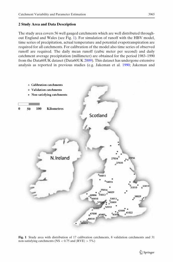
The study area covers 56 well gauged catchments which are well distributed through-out England and Wales (see Fig. 1). For simulation of runoff with the HBV model,time series of precipitation, actual temperature and potential evapotranspiration arerequired for all catchments. For calibration of the model also time series of observedrunoff are required. The daily mean runoff (cubic meter per second) and dailycatchment average precipitation (millimeter) are obtained for the period 1983–1990from the Data60UK dataset (Data60UK 2009). This dataset has undergone extensiveanalysis as reported in previous studies (e.g. Jakeman et al. 1990; Jakeman and

0 50 100 Kilometres

Fig. 1 Study area with distribution of 17 calibration catchments, 8 validation catchments and 31non-satisfying catchments (NS < 0.75 and |RVE| > 5%)


Hornberger 1993; Sefton and Howarth 1998). The study area includes moderatelydry up to wet catchments since the average annual rainfall over the period 1983–1990 ranges from less than 600 mm in east England to more than 2,100 mm inWales. Daily potential evapotranspiration has been estimated based on the formulaof Penman–Monteith, as recommended by the Meteorological Office for general usein the United Kingdom (Shaw 1994). This formula requires time series of actualtemperature, dew point temperature, sunshine hours and wind speed. These areobtained from observation stations throughout the United Kingdom originating fromthe British Atmospheric Data Centre (BADC 2009). For estimation of potentialevapotranspiration the two nearest observation stations which hold the datasetsfor actual temperature, dew point temperature and wind speed are used while forsunshine hours only the closest observation station is used. For the required dailytemperature, the same dataset is used as generated for estimation of the dailypotential evapotranspiration.

By the constraint to only use data that are available in the public domain, forderivation of PCCs the database of the National River Flow Archive (NRFA 2009)is used that is linked to the Catchment Spatial Information website (CSI 2009). Itmust be noted that by our selection the use of effective PCCs such as the BaseFlow Index (BFI) from the HOST data base is denied. BFIHOST for instance issuccessfully used in Young (2006) and Wagener and Wheater (2006). For selectionof PCC values, the boundaries of the catchments are based on regional topographicboundaries compiled through use of the Integrated Hydrological Digital TerrainModel (IHDTM) from the Centre for Ecology and Hydrology (CEH). Elevation isalso derived by application of the IHDTM which has a 50 m horizontal resolutionwith an elevation accuracy of 0.1 m. This resulted in catchments with sizes that varyfrom 25 up to 1,480 km2, where most catchments have an average elevation between100 and 200 m a.m.s.l. with 25.3 and 430.6 m a.m.s.l. as lowest and highest values in thedataset. Land use maps are derived from the Land Cover Map 2000 which is part ofthe Countryside Survey 2000 and 27 categories are identified. At the CSI pages theseare grouped into seven classes. In most catchments the dominating land use class is‘grassland’ with an average of 42.6%, followed by ‘arable’ and ‘woodland’ with valuesof respectively 30.4% and 13.4%. Geological maps are derived from the 1:625,000British Geological Survey datasets. A dataset with hydrogeological characteristicsthat affect river flow behaviour is used to make a distinction between permeable andimpermeable bedrock. In total, six classes are defined from impermeable bedrockto highly permeable bedrock. Wales generally contains very low permeable bedrockwhereas south, southeast and west England predominantly contain highly permeablebedrock.

3 Methodology

3.1 Hydrologic Model

The conceptual hydrologic model HBV is selected considering that it has many appli-cations in operational and strategic water management. The model has successfullybeen applied to catchments of various sizes and in a large range of geographic andclimatic settings. Applications in regionalisation studies are reported by, for instance,Seibert (1999), Merz and Blöschl (2004), Booij (2005) and Wale et al. (2009). The


Table 1 Model parameters and their minimum and maximum values used in the Monte Carlosimulation

Parameter Description Minimum Maximum

FC Maximum soil moisture storage (mm) 125 800BETA Parameter of power relationship to simulate indirect runoff (–) 1 4LP Limit above which evapotranspiration reaches its potential 0.1 1

value (–)ALFA Measure for non-linearity of flow in quick runoff reservoir (–) 0.1 3Kf Recession coefficient for runoff from quick runoff reservoir 0.0005 0.15

(per day)Ks Recession coefficient for runoff from base flow reservoir 0.0005 0.15

(per day)PERC Constant percolation rate occurring when water is available 0.1 2.5

(mm day−1)

model simulates river discharge and requires precipitation, actual temperature andpotential evapotranspiration as input. The HBV-96 model version (Lindström et al.1997) is used with a fixed time step of one day and in a spatially lumped way.The model used in this study consists of four routines, which are a precipitationaccounting routine, a soil moisture routine, a quick runoff routine and a base flowroutine which together transform excess water from the soil moisture zone into localrunoff. A full description of the HBV model is ignored for reasons of brevity andthe reader is referred to Lindström et al. (1997) and SMHI (1999). In Table 1 adescription of the model parameters is given.

The classical approach of regionalisation is applied and consists of three steps.First the HBV model is calibrated for 48 gauged catchments against observeddischarge in order to determine a well performing parameter set. Secondly, rela-tionships between sensitive model parameters and PCCs are established that makeup the so called ‘regional model’ and serves to estimate model parameters for theungauged catchments. Thirdly the HBV model is used to validate the regional modelfor the remaining eight ungauged catchments. In the following three sub-sections adescription of the three steps is given.

3.2 Calibration

3.2.1 Calibration and Selection of Parameters

For calibration of the HBV model Monte Carlo simulation (MCS) is applied to48 catchments. In MCS, simulations are executed for a large number of randomlygenerated parameter sets that are within a pre-defined parameter space. Modelperformance assessment is evaluated through an objective function or measure thatis an expression of fit between observed and simulated runoff hydrographs. Mostimportant in MCS is the selection of model calibration parameters, the determinationof prior parameter space, the selection of probability distributions for the calibrationparameters, the determination of the number of simulations to be executed and theselection of the objective function(s). For first applications of MCS simulation inhydrology we refer to Beven and Binley (1992) and Harlin and Kung (1992).

In this study we aim to develop a procedure that allows for simulation of variousaspects of the hydrograph. Therefore, a selection of HBV model parameters has tobe made that are sensitive to the various aspects. In studies by for instance Harlin and


Kung (1992), Lindström et al. (1997), Seibert (1999) and Booij (2005) such sensitivityis demonstrated and results of these studies are used for selection of model calibra-tion parameters. As such seven parameters are selected that require optimisationwhile for the remaining model parameters default values are used following SMHI(1999). The transformation routine that smoothes the instant runoff contributionsand the routing routine for linkage of upstream catchments are omitted.

Model parameter space is determined by evaluating model parameter rangesapplied in HBV studies by Bergström (1990), Booij (2005), Diermanse (2001),Harlin and Kung (1992), Killingtveit and Sælthun (1995), Lidén and Harlin (2000),Seibert (1999), SMHI (1999) and Velner (2000). Parameter values are randomly andindependently sampled from uniform distributions. In Table 1 the selected modelparameters and parameter ranges are given. For examination of the prior spaceof calibration parameters we selected a simulation run number of 10,000 (see alsoWagener and Wheater 2006).

3.2.2 Selection of Objective Functions

Madsen (2000) stated that for evaluation of a calibrated model usually four differentobjectives are considered. These are (1) a good water balance, (2) a good overallagreement of the shape of the hydrograph, (3) a good agreement of high flows and(4) a good agreement of low flows. In this work, for each of these objectives a (single)objective function (SOF) is defined that are the relative volume error (RVE) forassessing the goodness of fit for the water balance and the Nash–Sutcliffe coefficient(NS) (Nash and Sutcliffe 1970) for overall fit and high and low flows. The fourobjective functions are:

RVE =

⎛⎜⎜⎝

n∑i=1

Qsim(i) −n∑

i=1Qobs(i)

n∑i=1

Qobs(i)

⎞⎟⎟⎠ · 100% (1)

NS = 1 −

n∑i=1

(Qsim(i) − Qobs(i)

)2

n∑i=1

(Qobs(i) − Qobs(i)

)2(2)

NSH = 1 −

n∑i=1

Qobs(i) ≥ Qhigh


)2

n∑i=1

Qobs(i) ≥ Qhigh

(Qobs(i) − Qobs,high(i)

)2(3)

NSL = 1 −

n∑i=1

Qobs(i) ≤ Qtow


)2

n∑i=1

Qobs(i) ≤ Qlow

(Qobs(i) − Qobs,low(i)

)2(4)

where Qsim stands for simulated flow, Qobs for observed flow, Qobs(i) for the averageof observed flow, Qobs,high(i) for the average of observed flow above the selected high


discharge threshold Qhigh, Qobs,low(i) for the average observed flow below the lowdischarge threshold Qlow, i for the time step and n for the total number of time stepsused during calibration. RVE varies between −∞ and ∞ but performs best when avalue of 0 is generated. NS, NSH and NSL vary between −∞ and 1 and perform bestwhen a value of 1 is generated. Negative NS values indicate that the observed meandischarge is a better predictor than the model simulation. The simulation period isfrom January 1, 1983 to December 31, 1990. The first 8 months are selected as warm-up period and have not been used to calculate the SOF values. Threshold valuesfor low and high flow are arbitrarily defined as the 5-percentile and 90-percentileof exceeding probabilities. Selected percentiles suggest clear differentiation for thevarious catchment response modes that cause high and low flows.

3.2.3 Combination of Objective Functions

For the past decade, research on multi-objective model calibration revealed thattrade-offs exist between the different objectives and that, for instance, parametersets that yield good results for high flows may yield poor results for low flows. Toadequately simulate the different aspects of the stream flow hydrograph, trade-offsmust be evaluated to arrive at a well performing and robust parameter set thatfor selected objectives optimally performs. In this study a multi-objective function(MOF) is defined by combining all four SOFs. In the procedure each SOF contributesequally to the parameter optimisation problem where objective functions requirerescaling to allow for evaluation. Such evaluation should aim at selection of aparameter set that performs well for all SOFs. The likeliness that a parameter set withhighest performance for one SOF also performs best for a second SOF of a differentnature is questionable (see De Vos and Rientjes 2008). Therefore in this study we donot aim to select a best performing parameter set for one of the objectives but simplya parameter set that, presumably, performs well for all four selected performancemeasures. We hypothesize that such parameter set can be found in the selection of10% best performing parameter sets after rescaling. Alternatively, a non-preferencebased multi-objective method can be used that independently optimises multipleobjectives and reveals a set of solutions that represent the trade-off between theobjectives involved (i.e. a Pareto front, see e.g. Yapo et al. 1998; Khu and Madsen2005). The MOF used in this study implicitly balances the SOFs, which is in contrastto Pareto optimisation, where this is not necessary.

In this study for each catchment and for each SOF, the 1,000 best performing setswere used for rescaling. The best objective function value is the maximum NS, NSH

and NSL value and the minimum absolute RVE value out of 10,000 runs. The worstobjective function value is the 1,000th best calibration run for each SOF out of 10,000runs. For NS, NSH and NSL, for each calibration run the difference between thecalculated and the worst objective function value is divided by the difference betweenthe best and worst objective function values. For RVE., for each calibration runthe difference between the absolute values of the calculated and the best objectivefunction values is divided by the difference between the absolute values of the worstand best objective function values. Consequently, out of the 10,000 runs, rescaling ofthe SOF values resulted for the 1,000th best calibration run (worst objective functionvalue) in a value of 0 and for the best calibration run (best objective function value) ina value of 1. This implies that 90% of the 10,000 rescaled SOF values will be negative.For each run the minimum rescaled SOF value is selected out of the group of four


rescaled SOFs as expressed in Eq. 5 and is referred to as the minimum rescaled valueC′m.

C′m = Min

(CS−NS,m, CS−NSH ,m, CS−NSL,m, CS−RVE,m

)(5)

where CS stands for the rescaled SOF value and m for the calibration run number.For development of the regional model, the optimum parameter set Copt is nowdefined by selecting the maximum of the rescaled values C′

m:

Copt = Max(

C′m

∣∣ 1 ≤ m ≤ 10 000)

(6)

The selected parameter set is to be interpreted as a well performing or well behaving‘single best’ parameter set that, we hypothesise, is suitable for the development of theregional model. The above procedure differs from works by Wagener and Wheater(2006), Young (2006) and Parajka et al. (2007) since its optimisation is independentfor all four functions. In this respect our approach may be considered more pragmaticsince the final selection of the rescaled optimally performing parameter set is onlydependent on a single objective that may be different for the various catchments.While for one catchment NS may be highest for another catchment this may be NSH,NSL or RVE.. Principle to the approach is that we simply select a well performingparameter set for any one catchment that as such carries sufficient information to actas a descriptor of dominant hydrological characteristics of the catchment.

3.3 Establishing the Regional Model

The aim in determining the regional model is to establish statistically and hydrolog-ically relevant relationships between model parameters and PCCs. To achieve this,selections have to be made for the calibrated catchments to be used for establishingthe regional model and for the PCCs to be considered.

For the selection of calibration catchments two conditions are introduced: NS >

0.75 and |RVE| < 5%. We only used NS and RVE because these criteria have beenused in many other studies and allowed to reasonably define thresholds. Both condi-tions indicate that a model performs very well, although a high performance indicatornot (automatically) means that a model performs equally well on a catchment withlimited flow variation as compared to a catchment with highly variable flows. It isnoted that fulfilling both criteria has severely constrained the selection of catchments.For instance, preliminary results indicated that a NS larger than 0.6 would resultin some 35 out of 48 catchments. In many regionalisation studies (see e.g. Merzand Blöschl 2004; McIntyre et al. 2005; Young 2006; Duan et al. 2006; Parajkaet al. 2007; Oudin et al. 2008) the use of stringent criteria is advocated since such,presumably, allows selection of only those catchments for which a robust regionalmodel could be established. It is noted, however, that criteria in the previous worksare much more relaxed and commonly a NS efficiency of only 0.6 to 0.7 is used.Also, in Oudin et al. (2008) it is reported that poorly described catchments do notprovide sufficient relevant information. This has motivated our selection to apply thestringent performance criteria. Our selection has resulted in 17 catchments suitablefor establishing the regional model while 31 catchments are rejected. Relaxing theNS and RVE criteria would result in a much larger group of catchments suitablefor further use but, expectedly, also would result in introducing a wider range ofcatchment settings to the regional model. We note that this aspect of selecting


catchments for establishing the regional model touches on the (principle) discussionon effectiveness of regionalisation by the classical method but is further addressed inSection 5.

Selection of PCCs is based on previous research on regionalisation using HBV(i.e. Seibert 1999; Hundecha and Bárdossy 2004; Merz and Blöschl 2004) and theIHACRES model for catchments in England and Wales (Sefton and Howarth 1998)and on the availability of the data on PCCs in the public domain. This resulted inthe selection of 14 PCCs, classified into six groups as shown in Table 2. The PCCHI is a measure of the distribution of elevation in a catchment and is defined asthe average elevation a.m.s.l. minus the minimum divided by the difference betweenthe maximum and minimum elevation a.m.s.l. SHAPE is defined as the differencebetween the maximum and minimum elevation a.m.s.l. divided by the square rootof catchment size. Some statistics for each PCC and the average discharge, annualrainfall and annual potential evapotranspiration are shown in Table 3 and indicatewide ranges of climatic, topographic, geologic and land use settings. Whether thisvariability favours regionalisation could be questioned. This issue is also brieflyaddressed in Young (2006) and will be further discussed in Section 5.

For establishing relationships between model parameters and PCCs a simplecorrelation analysis has been performed with a significance level of α = 0.1. Scatterplots between model parameters and PCCs are evaluated to analyse non-linearityof relationships and regression analyses are performed in which the forward entrymethod and the backward removal method are applied. In the forward entry method,the established significant single relationships are extended by forcing additionalPCCs in the relationships until the last added PCC does not significantly contributeto the relationship. In the backward removal method, relationships incorporate allPCCs after which these ones are stepwise reduced until a significant relationshipis determined. Hereafter, the single and multiple relationships for each modelparameter are evaluated from a hydrological point of view since statistically sig-nificant relationships could possibly lack physical explanation. Finally, for eachmodel parameter a relationship is selected with one or more PCC(s), based on thestatistical significance (correlation coefficient of the relationship r) and on hydrologic

Table 2 Selected physical catchment characteristics (PCCs)

Group PCC Description

Dimension AREA Catchment size (km2)

Topography ELEVATION Catchment average elevation (m.a.s.l.)HI Hypsometric integral (–)

Shape SHAPE Catchment shape (–)Land use Wood Woodland (%)

Arable Arable and horticulture (%)Grass Grassland (%)Mountain Mountain, heath and bog (%)Urban Built-up areas (%)

Geology and soils HIGHP High permeability of bedrock (%)MODERATEP Moderate permeability of bedrock (%)LOWP Very low permeability of bedrock (%)MIXEDP Mixed permeability of bedrock (%)

Climate SAAR Standard annual average rainfall (mm)


Table 3 Statistics for each physical catchment characteristic (PCC) and average discharge (Q),annual rainfall (P) and annual potential evapotranspiration (PET) over the period 1983–1990

PCC/variable Unit Minimum 25 Percentile Median 75 Percentile Maximum

AREA km2 24.5 59.2 125.4 247.9 1480.0ELEVATION m.a.s.l. 25.3 116.3 141.1 215.5 430.6HI – 0.21 0.34 0.39 0.45 0.68SHAPE – 1.99 8.89 13.82 20.42 50.47Wood % 1.2 7.6 12.0 16.1 49.1Arable % 0.1 6.2 29.5 48.9 80.0Grass % 9.8 28.9 40.5 59.0 81.0Mountain % 0 0.4 1.8 7.3 63.6Urban % 0.2 1.8 3.2 6.1 74.0HIGHP % 0 0 0 53.0 100MODERATEP % 0 0 0 37.9 100LOWP % 0 0.7 42.5 84.0 100MIXEDP % 0 0 0 4.5 25.1Q m3 s−1 0.2 0.6 1.5 3.0 38.6SAAR = P mm year-1 573 703 825 1,175 2,173PET mm year−1 570 635 654 679 751

reasoning of the relationship. From this procedure only four PCCs (HI, HIGHP,LOWP and SAAR) could be identified that have significant effect on the establishedparameter set.

3.4 Validation

The regional model is validated based on the proxy-basin test (see Klemeš 1986)and eight gauged catchments are considered as pseudo ungauged. The establishedregional model is applied to these validation catchments for which model parametersets are generated. Out of 56 catchments, we selected eight catchments with sig-nificant hydrologic, climatic and physiographic diversity and distribution over theentire study area. For each of the four PCCs (i.e. HI, HIGHP, LOWP and SAAR)for which we assume they have a clear effect on runoff generation, we selectedtwo validation catchments that have PCC values closest to the 10-percentile and 90-percentile.

Performance of the regional model is assessed through the four non-scaled SOFvalues and by comparison of the four non-scaled SOF values of the regional para-meter set, a default parameter set and an optimum parameter set. For determinationof the optimum parameter set for the validation catchments the MCS methodologyas used for the calibration catchments is applied. The default parameter set uses thedefault values from SMHI (1999). It is noted that the default set must be interpretedas a generic descriptor of runoff behaviour for a wide range of climatic, topographicand physiographic settings. We denied establishing a default set as based on medianvalues of selected parameters (see e.g. Parajka et al. 2007; Oudin et al. 2008) since thedefault set suggests universal applicability. For missing default parameter values theaverage over the minimum and maximum values used in other research (i.e. the samenine studies as used for determining the parameter space) are calculated. The essenceof comparing the performance of the regional parameter set to the default parameterset is that the latter set will be used for application in ungauged catchments if theregional model fails to produce a realistic parameter set. To our knowledge such has


not been demonstrated before, but results in this work proved that the comparisonwas very effective to assess predictive capability of the regional model.

4 Results

4.1 Calibration

Following the calibration procedure a number of parameters could be well identifiedsince the model performed well within relatively small parameter space. The non-scaled SOF values for the optimum parameter sets for the 17 calibration catchmentsare shown in Table 4. Note that negative values are generated for the SOFs NSH

and NSL for respectively 2 and 15 catchments and indicate that the HBV model hasdifficulty in simulating low flow behaviour for these UK catchments (see Fig. 1). Itis noted that in NSL the error of the model is compared to the variance of observedlow flows. Since low flows generally have a very low variance, it is difficult to obtainsmall model errors compared to the observed variance, which often yields negativecriterion values.

Results also revealed that calibration for catchments with SAAR < 800 mm (i.e.dry catchments) failed since NS > 0.75 and | RVE| < 5% criteria have not been met.Also the mountainous catchments (Mountain > 17%) fail the calibration conditionswhich are practically all situated in the northern part of England. Furthermore, thecatchment with an exceptionally large built-up area (Urban = 61.3%) also failed theconditions. For 18 out of the 31 non-satisfying catchments NS values above 0.6 wereobtained. For 15 out of the 31 non-satisfying catchments it was possible to obtainNS values larger than 0.75. Thus, in a single objective perspective, the performanceof the model is actually overestimated when only considering the NS coefficient asperformance indicator, but also it could indicate that RVE is more restrictive thanNS.

Table 4 Seventeen calibration catchments with non-scaled single objective function values

Catchment NS(–) RVE(%) NSH(–) NSL(–)

27035 0.82 −1.10 −0.10 −1.8633019 0.75 1.54 0.38 −5.8541022 0.76 0.16 0.73 −3.6443006 0.80 −1.30 0.72 −19.7245005 0.78 −0.47 0.53 −73.5948003 0.87 −0.75 0.37 −3.2748010 0.94 −1.33 0.57 −3.6050001 0.81 −0.40 −2.24 −1.1352010 0.78 −4.14 0.60 −12.9353009 0.88 −4.02 0.67 −12.3854016 0.79 −1.91 0.36 −1.7954029 0.82 −1.53 0.54 −0.6655013 0.84 0.99 0.63 −3.4655014 0.89 −0.51 0.65 −1.5157010 0.88 0.66 0.16 0.3360006 0.85 −2.11 0.61 0.6366011 0.80 −4.20 −0.01 −0.04

Catchment numbers correspond with catchment observation stations as maintained at the NationalRiver Flow Archive



The correlation analyses resulted in significant correlations for 9 out of 98 rela-tionships between model parameters and PCCs (Table 5). The strongest correlationexists between evapotranspiration parameter LP and annual average rainfall SAARalthough such could be questioned from a hydrological point of view since SAARonly is defined at an annual scale thus ignoring the seasonal precipitation distributionwhile LP much more reflects on (actual) antecedent precipitation conditions. Analmost equally strong positive correlation is found between percolation parameterPERC and hypsometric integral HI-, that is justifiable based on Strahler (1952)and Merz and Blöschl (2004). For the quick recession coefficient Kf a considerablyweaker negative correlation is found with HI although a relation between the twocan be reasoned for. The remaining significant six correlations all concern modelparameter BETA related to indirect runoff. Three of these correlations relate to thePCC group land use, whereas the other three relate to respectively ELEVATION,SAAR andHIGHP (high permeability of bedrock).

Next, multiple regression analyses were performed. At first, multiple land useclasses were combined in a multiple regression equation and a relationship couldbe established for BETA. Through the forward entry method it was proved that thebest correlation could be established when land use classes Arable and Urban wereused. Application of the backward removal method did not lead to improvements inestimating BETA.

For parameter FC (maximum soil moisture storage) a significant relationshipcould be established by considering the PCCs Arable and HIGHP. In this relationhigher values for HIGHP resulted in a decrease of the maximum soil moisturestorage that is consistent with storage characteristics of bedrock material. Concerningparameter ALFA, determining the non-linearity of flow in the quick runoff reservoir,the multiple regression analysis resulted in only a significant relationship with thePCCs ELEVATION, HI and LOWP (very low permeability of bedrock). However,the hydrologic plausibility of the total relationship is questioned since the correlationwith ELEVATION and HI could not be explained. Regarding parameter Kf the

Table 5 Correlations between physical catchment characteristics and model parameters

FC BETA LP ALFA Kf Ks PERC

AREA −0.12 0.20 −0.12 −0.13 0.08 0.11 0.01ELEVATION −0.20 0.49 0.16 −0.32 0.37 0.26 −0.08HI 0.14 −0.08 −0.03 0.41 −0.44 −0.41 0.64SHAPE −0.03 0.10 0.26 −0.13 0.14 −0.07 0.03SAAR −0.04 0.48 0.65 −0.03 0.38 0.20 −0.20Wood −0.01 −0.04 −0.10 0.29 −0.13 0.30 −0.05Arable 0.21 −0.57 −0.31 0.09 −0.33 −0.37 0.21Grass −0.29 0.59 0.31 −0.20 0.33 0.235 −0.17Mountain 0.16 0.33 0.10 −0.06 0.08 0.189 −0.12Urban 0.17 −0.49 0.11 −0.03 0.23 −0.303 0.08HIGHP −0.07 −0.42 −0.23 0.06 −0.23 −0.147 0.13MODERATEP −0.15 −0.08 0.21 −0.26 0.37 0.152 −0.14LOWP 0.16 0.37 0.05 0.21 −0.11 0.037 −0.05MIXEDP 0.12 0.06 −0.27 −0.05 −0.25 −0.244 0.34

Values in italics are significant


Table 6 Selected relationships for definition of the regional model

Parameter Relationship Correlation, r

FC 1 / (0.0054 − 0.000105 × Arable + 0.0006685 × HIGHP) 0.64BETA 3.244 − 0.02328 × Arable − 0.09863 × Urban 0.67LP LN (1.568 + 0.000630 × SAAR) 0.69ALFA −0.06649 − 0.00155 × ELEVATION + 1.652 × HI + 0.65

0.00350 × LOWPKf 0.05866 + 0.000347 × ELEVATION − 0.274 × HI + 0.75

0.00775 × UrbanKs 0.0315 –PERC −0.595 + 5.615 × HI 0.64

Model parameters in italics are (partially) questioned based on hydrological interpretation

PCCs ELEVATION and Urban are added to the significant correlation with HI,together forming the strongest and most significant relationship which also is hydro-logically plausible. For parameter PERC the multiple regression analysis resulted ina relationship with several PCCs but, hydrologically, this relation can be questioned.

After evaluation of the established significant single and multiple regressionequations, for each model parameter the most plausible relationship is selectedbased on hydrologic reasoning and common understanding on the range of aspectsthat affects catchment runoff behaviour. These are shown in Table 6, in which therelationships belonging to the model parameters in italics are somehow questionablefrom a hydrologic point of view. For 6 out of 7 model parameters a relationship couldbe determined, whereas for the base flow parameter Ks no statistically significantrelationship was found. As a consequence and for simulating discharge at thevalidation catchments, the default value for Ks is used. For parameter PERC singleregression favoured multiple regression and as such PERC only will be related to HIin predicting runoff from ungauged catchments.

4.3 Validation

Application of the regional model to the validation catchments showed some out-comes that make the regionalisation approach in this study open to discussion.For instance it proved that some PCC values are outside the defined PCC spacebut also that some calculated model parameter values are outside the definedparameter space. Especially for parameter FC lower values are calculated than theminimum value and for 4 out of 8 validation catchments values lower than 60 mmare generated. For parameter Kf negative values are calculated for two catchments.This can be partly contributed to the fact that some regression relationships arequestionable from a hydrologic point of view (e.g. for FC). In this work, the actualPCC or calculated parameter value is replaced by the minimum or maximum PCCor parameter value if respective values lay outside PCC space or model parameterspace. The applied conditions resulted in adjusting 11 model parameter values for 6out of 8 validation catchments. Only three slight adjustments (about 10%) for PCCsELEVATION, HI and Arable have been implemented for two different catchments.

The resulting non-scaled SOF values for the optimum, regional and defaultparameter sets (see Section 3.2) for the eight validation catchments are given inTable 7. Validation shows that the regional parameter set in general performsdissatisfyingly. For 4 out of 8 validation catchments RVE values as generated with


the regional parameter set are comparable to the optimised SOF values. However,for the other four catchments the decrease in RVE values from the optimised modelto the regional model is very large, for example from 0.06% to 112.12% and from−0.49% to 85.77%. Thus, the regional model has difficulty in simulating the waterbalance. Concerning the calculated NS values, for two validation catchments (i.e.47008 and 53013) satisfying regionalised NS values are found that are comparableto optimum NS values. For the remaining catchments the decrease in general isconsiderable, i.e. at least 0.14. For the NSH and NSL values the decrease in modelperformance generated with the regional parameter set in general is larger, i.e. atleast 0.41. For most validation catchments negative optimised NSH and NSL valuesare generated indicating that the HBV model has difficulty in simulating high andlow flows correctly. It should be noted that the SOFs for high and particularly lowflows are primarily used to compare the model’s ability to simulate high and low flowbehaviour for different parameter sets to be used in the MOF. The absolute valuesof these SOFs should not be interpreted in the way regular NS values are interpreted(e.g. a value above 0.6 is satisfying and a value of 0.9 is very good).

When comparing the regionalised SOF values of the eight validation catchmentswith the values generated by the default parameter set as given in Table 7, it is shownthat both parameter sets perform comparatively. Out of a total of 32 generatedregionalised SOF values, 13 values are better than the SOF values generated with

Table 7 Non-scaled SOF values for the optimum parameter set, the regional model and the defaultparameter set for eight validation catchments

Catchment Parameter set NS (–) RVE(%) NSH(–) NSL(–)

27034 Optimum 0.75 −0.31 −0.25 −3.31Regional 0.55 −1.44 −5.10 −56.12Default 0.62 1.05 −0.30 −224.59

27056 Optimum −0.01 2.99 −2.80 −4.12Regional 0.08 −12.29 −3.28 −13.12Default −0.74 12.08 −2.61 −10.21


38029 Optimum 0.65 0.06 0.27 −21.26Regional −0.04 112.12 −0.14 −336.46Default 0.25 119.36 −0.04 −201.18

42008 Optimum 0.47 −0.49 −4.92 −1.18Regional −19.88 85.77 −310.83 −124.87Default −36.59 85.66 −308.23 −139.45


53013 Optimum 0.72 −7.90 −0.80 −10.40Regional 0.70 −6.31 −1.77 −50.23Default 0.79 −6.35 −0.60 −20.97

60010 Optimum 0.76 11.12 0.27 −0.69Regional 0.45 21.34 −0.15 −1.41Default −0.46 22.11 −1.02 −1.98

Values of the regional model in italics are lower than the values for the default parameter set


the default parameter set, whereas an improvement of model performance by theregional model was expected. For RVE, the regionalised and default values arecomparable although for one catchment the performance is considerably betterfor the regional model. For the regionalised NS values the default parameter setperforms better for five out of eight validation catchments and actually indicatesdeterioration of results of the regional model. Additionally, for the remaining threevalidation catchments the model performance is disappointing (i.e. values of −19.88,0.08 and 0.45). With respect to NSH the default parameter set performs better forseven out of eight validation catchments. The regional parameter set performs betterfor NSL for four out of eight validation catchments as compared to the defaultparameter set. The performance of the default set in general is disappointing withvalues of −124.87 and −70.17. There is only one validation catchment (60010) forwhich the regional parameter set performs better for all four SOFs as compared tothe default parameter set.

Figure 2 shows the observed and modelled hydrograph with the regional andoptimum parameter set for two validation catchments to illustrate performance of

0

1

2

3

4

5

6

7

8

1987 1988 1989

Observed

Regional

Optimum

0

100

200

300

400

500

600

1987 1988 1989

Dis

char

ge (

m3 /s

)

Observed

Regional

Optimum

(a)

(b)

Fig. 2 Observed discharge and modelled discharge with regional and optimum parameter set forvalidation catchments 38029 (a) and 60010 (b) for the period 1987–1989


Table 8 Non-scaled SOF values for the optimum parameter set, the regional model and the defaultparameter set for 18 non-satisfying calibration catchments with NS values above 0.6



22006 Optimum 0.63 2.07 −0.88 −2.47Regional 0.22 −14.36 −8.90 −1480.24Default 0.62 24.94 −0.77 −902.41

23006 Optimum 0.72 −1.89 −1.76 −2.12Regional 0.48 0.65 −10.50 −3.09Default 0.68 3.11 −2.85 −3.40

24004 Optimum 0.61 −8.15 −1.54 −2.17Regional 0.43 −20.38 −4.50 −26.86Default 0.59 −10.55 −1.87 −4.88

25005 Optimum 0.69 2.54 0.26 −1.59Regional 0.65 −12.53 −0.56 −5.48Default 0.66 5.04 −0.16 −14.54


27042 Optimum 0.67 −2.98 0.12 −0.42Regional 0.57 −15.03 −0.76 −11.57Default 0.59 −5.37 −0.05 −1.14

28008 Optimum 0.75 −1.79 0.64 −6.90Regional 0.72 −5.10 0.32 −83.20Default 0.59 −1.28 −0.30 −23.57

30015 Optimum 0.68 −1.21 −2.77 0.24Regional 0.49 29.40 −0.70 −33.42Default −0.60 32.76 −13.35 −14.77


32004 Optimum 0.65 −4.10 0.27 −0.04Regional 0.43 0.58 −4.24 −76.68Default 0.77 12.21 0.53 −6.27

32006 Optimum 0.73 −2.71 0.24 −2.38Regional 0.53 −3.92 −3.19 −44.71Default 0.68 23.42 −0.41 −9.36

33029 Optimum 0.70 −0.41 −0.66 −2.20Regional −0.55 55.33 −9.55 −338.11Default −0.76 62.23 −13.46 −315.50

36003 Optimum 0.69 1.11 0.81 −1.61Regional 0.45 44.81 0.55 −5.96Default 0.66 39.06 0.77 −7.31

49002 Optimum 0.86 −7.32 0.47 −13.77Regional 0.44 −24.36 −1.09 −14.26Default 0.08 −10.69 −0.68 −48.87

53017 Optimum 0.80 −4.54 0.07 −2.56Regional 0.83 −0.94 0.26 −10.94Default 0.85 0.50 0.42 −31.13


Table 8 (continued)


62001 Optimum 0.84 −6.21 0.01 0.37Regional 0.66 −8.74 0.37 0.38Default 0.50 −6.84 0.15 −6.34

67018 Optimum 0.73 −4.71 −1.47 0.70Regional 0.70 −5.77 −1.58 −0.63Default 0.67 −6.37 −1.78 0.87

Values of the regional model in italics are lower than the values for the default parameter set

the regional model. For one catchment (38029, see Table 7) the regional parameterset results in very poor performance while the optimum parameter set shows areasonable simulation. For the other catchment (60010) the regional parameter setshows performance in line with the optimum performance. The regional modelclearly does not capture the discharge peaks and largely overestimates the dischargefor average and low flow periods (see also the RVE value in Table 7) for catchment38029. This is probably caused by the small ALFA and Kf values as predicted by theregional model compared to the optimum values for these parameters. The originalKf value as predicted by the regional model was negative and had to be adjusted tothe minimum Kf value as obtained in the calibration. The regionalisation relationshipfor ALFA can be (partially) questioned based on hydrological interpretation (seeTable 6). Although the regional model slightly overestimates discharge variabilityand peaks for catchment 60010, the general discharge behaviour is well simulated andcomparable with the discharge behaviour as simulated with the optimum parameterset.

An additional validation is done using a sub-set of the non-satisfying calibrationcatchments with a NS value above 0.6. This resulted in 18 additional catchmentsavailable for validation since these catchments have not been used for calibrationpurposes (see Section 4.1). Table 8 shows the resulting non-scaled SOF valuesfor the optimum, regional and default parameter sets for these catchments. Theadditional validation runs for 18 catchments generally shows similar results as forthe validation with 8 catchments. For 6 out of 18 catchments for NS and for 8 outof 18 catchments for RVE, SOF values as generated with the regional parameter setare comparable to the optimised SOF values. Results for NSH and NSL are similar orpoorer as compared to the results for the validation catchments. Default sets performequally or slightly better than regional parameter sets. Out of a total of 72 generatedregionalised SOF values, 26 values are better than the SOF values generated with thedefault parameter sets. These additional validation results are in line with the originalvalidation results and indicate dissatisfying performance of the regional model.

5 Discussion

In this study, 31 out of 48 catchments could not be satisfactory calibrated by verystringent criteria and are ignored for establishing regional relationships that make


up the regional model. Model calibration was performed through MCS on fourcomplementary objective functions that independently have been optimised. Forrunoff simulation the HBV model has been selected as also applied by for instanceSeibert (1999) and Merz and Blöschl (2004).

5.1 Calibration

As described, in this work calibration and validation results in general were notsatisfying and regionalised model parameters did not allow to accurately simulatea large number of catchments. Clear reasons for disappointing model performancecould not be identified, although possible causes relate to the input of inaccuratemeteorological forcing data, inadequate multi-objective optimization, insufficienciesin the model structure of the HBV model, inadequate selection of PCCs and weaklydefined regionalisation relations.

Selection of calibration catchments to be used for regionalisation is based onpredefined values of the objective functions that assess the overall fit of observedand simulated hydrographs. By (very) constraining performance criteria of NS > 0.75and RVE of <5% this selection resulted in only 17 catchments and could suggest thatthe HBV model has some insufficiencies. It must be noted however that successfulapplications are reported in literature in a wide range of climatic and topographicsettings (see Lidén and Harlin 2000; Booij 2005; Akhtar et al. 2008, 2009; Waleet al. 2009). Thus the small number could indicate that, in particular, meteorologicalforcing by precipitation and evapotranspiration is poorly represented. An inappro-priate model structure as well as poor representation of meteorological forcingare also identified in Young (2006) as possible cause of disappointing results of aregionalisation approach for 260 catchments in the UK.


Principle to our regionalisation procedure is that PCCs to be used in the regionalmodel are assumed to be of relevance to describe catchment runoff. By regressionanalysis, in this work it is shown that for only few PCCs statistically significant rela-tionships could be established with selected HBV model parameters. Although eachof the PCCs has some hydrological relevance, effects on how these PCCs affect quickflow and how much runoff is produced through saturation and infiltration excessmechanisms could not be shown. In using PCCs in regionalisation it must be realisedthat detailed real world information that largely affects runoff dynamics is ignored(as in the model). Duan et al. (2006) describe results of the MOPEX experiment andindicates that much research is needed to understand how model parameters relateto basin characteristics. Also it is described that ‘observable’ characteristics, that alsoare used in this study, may not be the most relevant descriptors of factors that controlrunoff production and runoff behaviour. In this research however we were not ableto prove ineffectiveness of selected PCCs since such would require that effects ofselected PCCs on runoff prediction can be isolated. Possibly the limited hydrologicalinterpretability of the PCC causes that PCCs are not effective for all catchments.

Application of the regional model to eight validation catchments indicated disap-pointing performance and the established model parameter sets could not satisfac-tory predict runoff. An additional validation using a sub-set of the non-satisfying


calibration catchments indicated similar results. For some catchments establishedparameter values fall outside earlier established minimum or maximum values. Inthe procedure it appears that assumed relationships between model parameters andPCCs are weak which results in unrealistic parameter values. As such the validity ofthe established regionalisation relations can be questioned and predictive capabilityonly is poor. Overall it can be concluded that simulation results from regional anddefault parameter sets are comparable, which indicate that the established regionalmodel has no universal validity for the catchments throughout the UK. Such isalso shown in Young (2006) where it is described that catchments in the southof the UK are dominated by their groundwater flow regime and that for thesecatchments the water balance could not be closed. In the same work, for catchmentstowards the east coast of Scotland that are considered ‘dry’, the regionalisationfailed since precipitation input is very poor due to a sparse rain gauge network.Similar conclusions in this paper cannot be drawn by the relatively small numberof catchments used for validation.

5.3 Catchment Variability

In the regionalisation approach in this study it is assumed that optimised modelparameters that represent certain catchment characteristics are applicable to othercatchments as well in case catchment settings are comparable. Such settings, how-ever, always are subject to variability and important is the question to which extentvariability favours regionalisation. Little variation implies little hydrologic diversitythat does allow establishment of strong regional relationships applicable to a limitednumber of catchments, while too much variation may result in weak relationships(more generally applicable). In Seibert (1999) a successful application of the HBVmodel is described for some 11 catchments that are characterised by only little vari-ation in settings. Haberlandt et al. (2001) favour the assumption of large variabilityand a clear range of different conditions is advocated as basis for regionalisation.Work by Young (2006) on 260 catchments distributed across the entire UK showedthat regionalisation in general was successful although results also indicate failure forcatchments under dry climatic settings. Our approach in general was not successfulalthough regionalisation was based on optimal parameter sets as defined by fourobjective functions. Possibly the entire data set carries too much variability to beeffectively used for regionalisation. Differences in the above mentioned approachesare the procedure to select optimal parameters and the selected PCCs. This studyonly used PCCs from the National River Flow Archive that are available throughCSI (2009). Concluding that PCCs are inappropriate or that optimal parameter setsare wrongly defined cannot be simply reasoned for. It must be noted that the baseflow index as effective PCC in Young (2006), Kay et al. (2006), McIntyre et al. (2005)and Wagener and Wheater (2006) was not used in this study, but obviously has(very) positively affected the outcomes of these works. The latter work consideredonly 10 catchments in south east England with, presumably, much less variability.Also Wagener and Wheater (2006) report on statistical regionalisation while againa number of different PCCs are selected. Results from that work with a simpleconceptual model structure are satisfying although it is stated that the approach isunlikely to be robust because of the small number of catchments.


6 Conclusions

In this study the classical approach of regionalisation is applied to a set of 56catchments in England and Wales in order to assess predictive capability of a regionalmodel in simulating runoff at assumed ungauged catchments. For runoff simulationat calibration and validation catchments the HBV model is used. Optimal parametersets are established by considering a combination of four single objective functionsand MCS. Our approach was to establish relationships between optimised parametersets and PCCs, and for six out of seven selected model parameters statisticallysignificant relationships could be derived three of which are hydrologically plausible.For the seventh model parameter a default parameter value is used to complete theregional model.

Validation of the regional model at eight catchments revealed that the perfor-mance is not satisfactory. The difference in performance of the regional model andthe optimum parameter set was larger than expected for most catchments. Alsosome default parameter values perform better than regionalised parameter values.Results show that default parameter sets outperformed regional parameter sets for19 out of 32 single objective function values for the validation catchments. Similarresults were obtained by additional validation runs using a sub-set of catchments notused in the regionalisation. It is concluded that regionalisation in this research wasnot successful and that predictive capability of the established regional model couldnot be improved. Identification of causes for the disappointing performance of theproposed regionalisation approach indicated that performance was due to a numberof causes. Quantification of each of these causes however was not possible due to thecomplexity and interdependencies of causes.

Further research on the classical approach of regionalisation should focus on therelation between model parameters and PCCs. Different (local) model structureswith the same set of PCCs and vice versa, different PCCs for the same modelstructure could be tested to identify appropriate model structures and accompanyingPCCs when using the classical approach. Moreover, PCCs and model parameterscould be more adapted to each other by constructing PCCs describing the runoffformation process as simulated by the model, and by adapting or developing modelstructures incorporating observable ‘PCCs’. Alternatively, other regionalisation ap-proaches can obviously be tested and compared to the classical approach using thesame model structure for similar climatic and geographical conditions.

Acknowledgements The authors are grateful to the British Atmospheric Data Centre whichprovided us with access to the Met Office Land Surface Observation Stations Data, the Top Downmodelling Working Group within the PUB initiative for the hydrometric data and the National RiverFlow Archive for all physiographic data.

Open Access This article is distributed under the terms of the Creative Commons AttributionNoncommercial License which permits any noncommercial use, distribution, and reproduction inany medium, provided the original author(s) and source are credited.

References

Abdulla F, Eshtawi T, Assaf H (2009) Assessment of the impact of potential climate change on thewater balance of a semi-arid watershed. Water Resour Manag 23:2051–2068


Akhtar M, Ahmad N, Booij MJ (2008) The impact of climate change on the water resources ofHindukush–Karakorum–Himalaya region under different glacier coverage scenarios. J Hydrol355:148–163

Akhtar M, Ahmad N, Booij MJ (2009) Use of regional climate model simulations as input forhydrological models for the Hindukush–Karakorum–Himalaya region. Hydrol Earth Syst Sci13:1075–1089

Ao T, Ishidaira H, Takeuchi K, Kiem AS, Yoshitari J, Fukami K, Magome J (2006) RelatingBTOPMC model parameters to physical features of MOPEX basins. J Hydrol 320:84–102

BADC (2009) British atmospheric data centre. http://badc.nerc.ac.uk. Accessed 17 November 2009Bergström S (1990) Parameter values for the HBV model in Sweden (in Swedish). Technical Report

no. 28. SMHI, NorrköpingBergström S (1995) The HBV model. In: Singh VP (ed) Computer models of watershed hydrology.

Water Resources Publications, Highlands Ranch, pp 443–476Beven K, Binley A (1992) The future of distributed models: model calibration and uncertainty

prediction. Hydrol Process 6:279–298Blöschl G, Sivapalan M (1995) Scale issues in hydrological modelling: a review. Hydrol Process

9:251–290Booij MJ (2005) Impact of climate change on river flooding assessed with different spatial model

resolutions. J Hydrol 303:176–198CSI (2009) Catchment spatial information. http://www.ceh.ac.uk/data/nrfa/catchment_spatial_

information.html. Accessed 17 November 2009Cutore P, Cristaudo G, Campisano A, Modica C, Cancelliere A, Rossi G (2007) Regional models for

the estimation of streamflow series in ungauged basins. Water Resour Manag 21:789–800Data60UK (2009) Eleven-year records (1980–1990) of continuous daily catchment precipitation

and mean streamflow for 61 catchments throughout England and Wales. http://www.nwl.ac.uk/ih/nrfa/pub/index.html. Accessed 17 November 2009

De Vos NJ, Rientjes THM (2007) Multi-objective performance comparison of an artificial neuralnetwork and a conceptual rainfall–runoff model. Hydrol Sci J 52:397–413

De Vos NJ, Rientjes THM (2008) Multi-objective training of artificial neural networks for rainfall–runoff modeling. Water Resour Res 44:W08434

Diermanse FLM (2001) Physically based modelling of rainfall–runoff processes. PhD thesis. DelftUniversity Press, Delft

Duan Q, Schaake J, Andréassian V, Franks S, Goteti G, Gupta HV, Gusev YM, Habets F,Hall A, Hay L, Hogue T, Huang M, Leavesley G, Liang X, Nasonova ON, Noilhan J, Oudin L,Sorooshian S, Wagener T, Wood EF (2006) Model parameter estimation experiment (MOPEX):an overview of science strategy and major results from the second and third workshops. J Hydrol320:3–17

Engeland K, Hisdal H (2009) A comparison of low flow estimates in ungauged catchments usingregional regression and the HBV-model. Water Resour Manag 23:2567–2586

Gupta HV, Sorooshian S, Yapo PO (1998) Toward improved calibration of hydrologic models:multiple and noncommensurable measures of information. Water Resour Res 34:751–763

Gupta HV, Wagener T, Liu Y (2008) Reconciling theory with observations: elements of a diagnosticapproach to model evaluation. Hydrol Process 22:3802–3813

Haberlandt U, Klöcking B, Krysanova V, Becker A (2001) Regionalisation of the base flow indexfrom dynamically simulated flow components—a case study in the Elbe River Basin. J Hydrol248:35–53

Harlin J, Kung C (1992) Parameter uncertainty and simulation of design floods in Sweden. J Hydrol137:209–230

Hundecha Y, Bárdossy A (2004) Modelling of the effect of land use change on the runoff gener-ation of a river basin through parameter regionalization of a watershed model. J Hydrol 292:281–295

Jakeman AJ, Hornberger GM (1993) How much complexity is warranted in a rainfall–runoff model?Water Resour Res 29:2637–2649

Jakeman AJ, Littlewood IG, Whitehead PG (1990) Computation of the instantaneous unit hy-drograph and identifiable component flows with application to two small upland catchments.J Hydrol 117:275–300

Kay AL, Jones DA, Crooks SM, Calver A, Reynard NS (2006) A comparison of three approachesto spatial generalization of rainfall–runoff models. Hydrol Process 20:3953–3973

Killingtveit A, Sælthun NR (1995) Hydropower development: hydrology. Technical report.Norwegian Institute of Technology, Oslo

http://badc.nerc.ac.uk

http://www.ceh.ac.uk/data/nrfa/catchment_spatial_information.html

http://www.ceh.ac.uk/data/nrfa/catchment_spatial_information.html

http://www.nwl.ac.uk/ih/nrfa/pub/index.html

http://www.nwl.ac.uk/ih/nrfa/pub/index.html


Khu ST, Madsen H (2005) Multiobjective calibration with Pareto preference ordering: an applicationto rainfall–runoff model calibration. Water Resour Res 41:W03004

Klemeš V (1986) Operational testing of hydrological simulation models. Hydrol Sci J 31:13–24Kokkonen T, Jakeman A, Young P, Koivusalo H (2003) Predicting daily flows in ungauged

catchments: model regionalization from catchment descriptors at the Coweeta HydrologicLaboratory, North Carolina. Hydrol Process 17:2219–2238

Lidén R, Harlin J (2000) Analysis of conceptual rainfall–runoff modelling performance in differentclimates. J Hydrol 238:231–247

Lindström G, Johansson B, Persson M, Gardelin M, Bergström S (1997) Development and test ofthe distributed HBV-96 hydrological model. J Hydrol 201:272–288

Madsen H (2000) Automatic calibration of a conceptual rainfall–runoff model using multipleobjectives. J Hydrol 235:276–288

McIntyre N, Lee H, Wheater H, Young A (2005) Ensemble predictions of runoff in ungaugedcatchments. Water Resour Res 41:W12434

Merz R, Blöschl G (2004) Regionalisation of catchment model parameters. J Hydrol 287:95–123Moore RJ (1985) The probability-distributed principle and runoff production at point and basin

scales. Hydrol Sci J 30:273–297Moore RJ (1999) Real-time flood forecasting systems: perspectives and prospects. In: Casale R,

Margottini C (eds) Floods and landslides: integrated risk assessment. Springer, Berlin,pp 147–189

Nash JE, Sutcliffe JV (1970) River flow forecasting through conceptual models. Part I - A discussionof principles. J Hydrol 10:282–290

NRFA (2009) National River Flow Archive. http://www.ceh.ac.uk/data/nrfa/index.html. Accessed 17November 2009

Oudin L, Andréassian V, Perrin C, Michel C, Le Moine N (2008) Spatial proximity, physical simi-larity, regression and ungaged catchments: a comparison of regionalization approaches based on913 French catchments. Water Resour Res 44:W03413

Parajka J, Blöschl G, Merz R (2007) Regional calibration of catchment models: potential forungauged catchments. Water Resour Res 43:W06406

Sefton CEM, Boorman DB (1997) A regional investigation of climate change impacts on UKstreamflows. J Hydrol 195:26–44

Sefton CEM, Howarth SM (1998) Relationships between dynamic response characteristics andphysical descriptors of catchments in England and Wales. J Hydrol 211:1–16

Seibert J (1997) Estimation of parameter uncertainty in the HBV model. Nord Hydrol 28:4–5Seibert J (1999) Regionalisation of parameters for a conceptual rainfall–runoff model. Agric For

Meteorol 98–99:279–293Shaw EM (1994) Hydrology in practice, 3rd edn. Chapman & Hall, LondonSivapalan M, Takeuchi K, Franks SW, Gupta VK, Karambiri H, Lakshmi V, Liang X, McDonnell

JJ, Mendiondo EM, O’Connell PE, Oki T, Pomeroy JW, Schertzer D, Uhlenbrook S, Zehe E(2003) IAHS decade on predictions in ungauged basins (PUB), 2003-2012: shaping an excitingfuture for the hydrological sciences. Hydrol Sci J 48:857–880

SMHI (1999) Integrated hydrologic modelling system (IHMS). Manual version 4.3. SMHI,Norrköping

Strahler AN (1952) Hypsometric (area-altitude) analysis of erosional topography. Geol Soc AmerBull 63:1117–1141

Tang Y, Reed P, Wagener T (2006) How effective and efficient are multiobjective evolutionaryalgorithms at hydrological model calibration? Hydrol Earth Syst Sci 10:289–307

Velner RGJ (2000) Rainfall–runoff modelling of the Ourthe catchment with the HBV model. Astudy for extension of the lead time for flood forecasting in the Meuse (in Dutch). RIZA workingdocument 2000.091X. Wageningen University, Wageningen

Verbunt M, Zwaaftink MG, Gurtz J (2005) The hydrological impact of land cover changes andhydropower stations in the Alpine Rhine basin. Ecol Model 187:71–84

Wagener T, Wheater HS (2006) Parameter estimation and regionalization for continuous rainfall–runoff models including uncertainty. J Hydrol 320:132–154

Wagener T, Lees MJ, Wheater HS (2002) A toolkit for the development and application of par-simonious hydrological models. In: Singh VP, Frevert D (eds) Mathematical models of largewatershed hydrology, vol 1. Water Resources Publications, Highlands Ranch, pp 87–136

Wagener T, Wheater HS, Gupta HV (2003) Identification and evaluation of watershed models. In:Duan Q, Gupta HV, Sorooshian S, Rousseau AN, Turcotte R (eds) Calibration of watershedmodels. Water Science and Application 6, American Geophysical Union, pp 29–47

http://www.ceh.ac.uk/data/nrfa/index.html


Wale A, Rientjes THM, Gieske ASM, Getachew HA (2009) Ungauged catchment contributions toLake Tana’s water balance. Hydrol Process 23:3682–3693

Yadav M, Wagener T, Gupta H (2007) Regionalization of constraints on expected watershed re-sponse behavior for improved predictions in ungauged basins. Adv Water Resour 30:1756–1774

Yapo PO, Gupta HV, Sorooshian S (1998) Multi-objective global optimization for hydrologicmodels. J Hydrol 204:83–97

Young AR (2006) Stream flow simulation within UK ungauged catchments using a daily rainfall–runoff model. J Hydrol 320:155–172

Zhang YQ, Chiew FHS (2009) Relative merits of different methods for runoff predictions inungauged catchments. Water Resour Res 45:W07412

catchment variability and parameter estimation in …...catchment variability and parameter...

Documents