congetion control.pptx

Congestión Control

Presented By: Naveen Kr. Dubey NITTTR, Chandigarh

Congestion…?

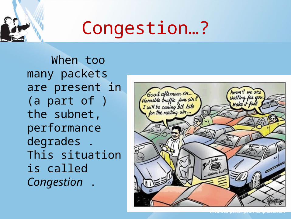
When too many packets are present in (a part of ) the subnet, performance degrades . This situation is called Congestion .

Network Congestion(Cont’d)

Packet dumped by hosts on subnet within the carrying capacity.

Almost 100% delivery No of delivered packet is

proportional to no of packet sent.

Packet dumped on subnet to far from carrying capacity

Router are no longer able to cope.

Packet losing starts. At very high traffic ,

performance collapse completely and almost no packet delivered.

Network Congestion(Cont’d)

Factors Influencing ?

If all of sudden, stream of packet begin arriving on three or four input lines and all needs the same output line, A queue will build up. If there is insufficient memory to hold all of them, packets

will get lost.

Nagle J: “Congestion control in TCP/IP Internetworks,” Computer Commun. Rev. , vol 14, pp. 11-17, April 1987

If the router have infinite amount of memory, congestion gets worse, not better, because by the time packet get to the front of the queue, they have already timed out. Duplicate have been sent which further increase traffic load.

Factors Influencing ?(Cont’d)

Slow processor can also cause congestion . If CPU is slow in book keeping task (like queuing buffers, updating tables etc.) Queue build up even there is excess line capacity.

Low bandwidth line also cause congestion.

Congestion leads to feed upon itself

Congestion tends to feed upon itself to get even worse. Routers respond to overloading by dropping packets. When these packets contain TCP segments, the segments don't reach their destination, and they are therefore left unacknowledged.

which eventually leads to timeout and retransmission.

The major cause of congestion is often the bursty nature of traffic.

If the hosts could be made to transmit at a uniform rate, then congestion problem will be less common and all other causes will not even led to congestion

because other causes just act as an enzyme which boosts up the congestion when the traffic is bursty

Flow Control & Congestion Control

There is subtle relation between Congestion control and Flow control. Objective of Congestion control is to ensure the

subnet is able to carry the offered traffic. It is a global issue involving the behavior of all hosts, all

the routers, the store and forward processing in routers and all other parameters tending to diminish the capacity of subnet.

Flow control is concerned about point-to-point link between sender and receiver . Its job is to make sure that a fast sender can not

transmit data faster than the receiver can absorb it. It always involve some direct feedback .

The Congestion control and Flow control are often confused because some congestion control algorithms operate by sending message back to the various sources telling them to slow down when the network gets into trouble.

Thus a host get a “slow down” message either because the receiver can not handle the load, or because network can’t handle it.

Principles of Congestion Control

Congestion control refers to technique and mechanism that can either prevent congestion, before it happens, or remove congestion, after it has happened.

The presence of congestion means that the load is (temporarily) greater than the resource (in part of system) can handle it.

Two solution comes in mind: increase the resource or decrease the load.

Many congestion control algorithms are known

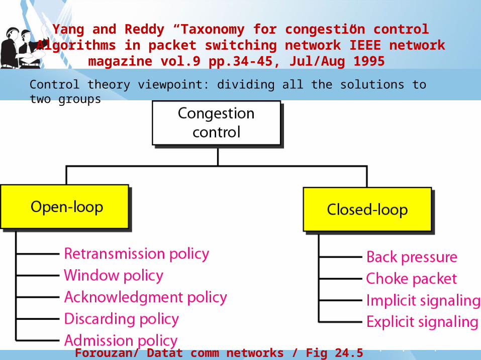
Yang and Reddy “Taxonomy for congestion control Algorithms in packet switching network”IEEE network

magazine vol.9 pp.34-45, Jul/Aug 1995

Forouzan/ Datat comm networks / Fig 24.5

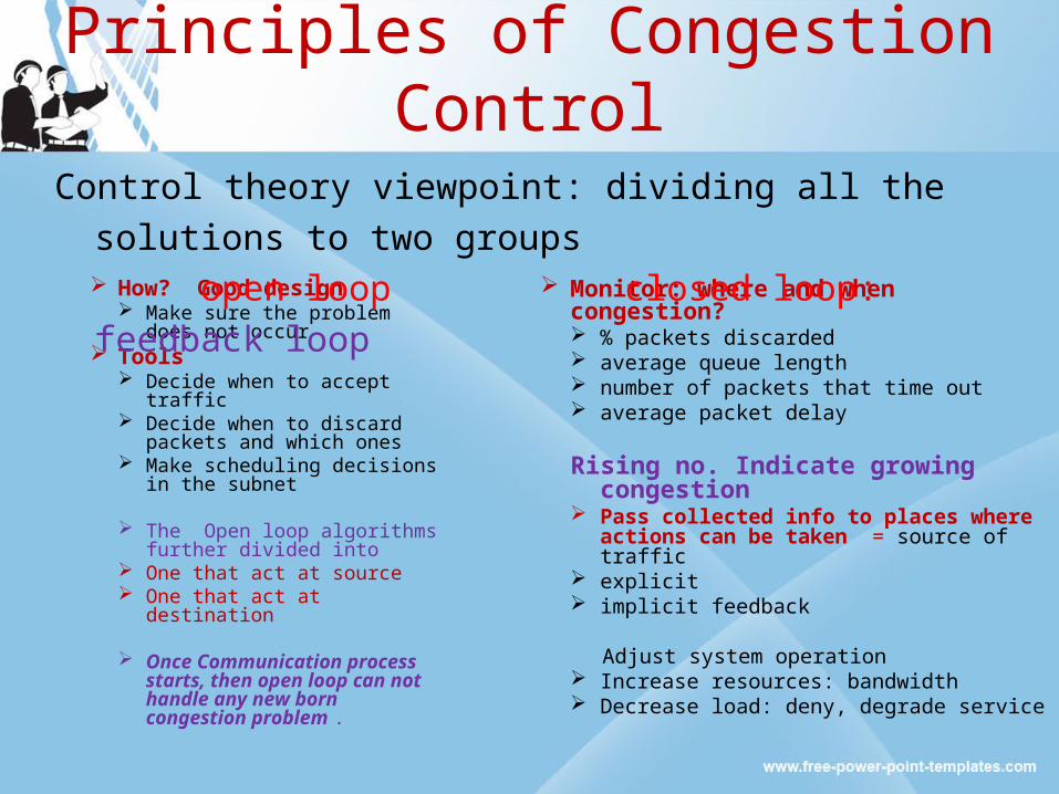
Control theory viewpoint: dividing all the solutions to two groups

Principles of Congestion Control(Open Loop)

Tools for doing open loop control include

deciding. When to accept new traffic ? When to discard packet and which one ? Making scheduling decision at various point in the

network .

All of these have in common the fact that they make decision without regard to the current state of the network.

Principles of Congestion Control(Closed loop)

Closed loop solutions are based on the concept of a feedback loop.

This approach includes three parts when applied to congestion control Monitor the system when and where the congestion

occurs . Pass this information to place where action can be

taken. Adjust system operation to correct the problem.

Principles of Congestion Control

How? Good design Make sure the problem does

not occur Tools

Decide when to accept traffic Decide when to discard

packets and which ones Make scheduling decisions

in the subnet

The Open loop algorithms further divided into

One that act at source One that act at destination

Once Communication process starts, then open loop can not handle any new born congestion problem .

Monitor: where and when congestion? % packets discarded average queue length number of packets that time out average packet delay

Rising no. Indicate growing congestion

Pass collected info to places where actions can be taken = source of traffic

explicit implicit feedback

Adjust system operation Increase resources: bandwidth Decrease load: deny, degrade service

Control theory viewpoint: dividing all the solutions to two groups

open loop closed loop: feedback loop

Cont’d…

In implicit algorithms the source deduce the existence of congestion by making local observations, such as time needed for acknowledgment to come back.

(when router detect this is congested state it fills in the field of all outgoing packets to warn the neighbors )

In explicit algorithms host or router send probe packets out periodically to ask about congestion

( For some radio station helicopter flying around the city to update traffic info)

Principles of Congestion Control(Time Scale Adjustment )

Time scale must be adjusted carefully, to work well some kind of averaging needed but getting the time constant right is a

non trivial matter . Example: Suppose there is certain set of instruction

1. When two packet comes in a row:

Router yells STOP.

2. Every time router idle for 20 µs : yells GO

(System will oscillate wildly and never converge ) On the other hand : If waits for 30 minute to make sure

before

saying anything

(system will react sluggishly for any real use)

Congestion: prevention Policies open loop solutions: Minimize congestion, they try to achieve there goals by

using appropriate policies at various levels

Layer Policies

Transport Retransmission policy Out-of-order caching policy Acknowledgement policy Flow control policy Timeout determination ( transit time over the network is hard to predict)

Network Virtual circuits <> datagrams in subnet( many cog. Control algo work only with VC) Packet queueing and service policy ( 1 Q / input/output line and round robin) Packet discard policy Routing algorithm ( spreading traffic over all lines) Packet lifetime management

Data link Retransmission policy( Go back N will put heavy load than Selective Reject) Out-of-order caching policy ( Selective repeat is better ) Acknowledgement policy( piggyback onto reverse traffic ) Flow control policy ( small window reduce traffic and thus congestion )

Types of Congestion Control

Preventive The hosts and routers attempt to prevent

congestion before it can occur Reactive

The hosts and routers respond to congestion after it occurs and then attempt to stop it

Preventive Techniques: Resource reservation Leaky/Token bucket

Reactive Techniques: Load shedding Choke packets

Traffic-Aware Routing

To make the most of the existing network capacity, routes can be tailored to traffic patterns that change during the day as network users wake and sleep in different time zones.

For example: routes may be changed to shift traffic away from

heavily used paths by changing the shortest path weights.

This is called traffic-aware routing. Splitting traffic across multiple paths is also helpful.

Traffic-Aware Routing

The routing schemes we looked at in used fixed link weights.

These schemes adapted to changes in topology, but not to changes in load.

The goal in taking load into account when computing routes is to shift traffic away from hotspots that will be the first places in the network to experience congestion.

The most direct way to do this is to set the link weight to be a function of the(fixed) link bandwidth and propagation delay plus the (variable) measured load or average queuing delay. Least-weight paths will then favour paths that are more lightly loaded, all else being equal.

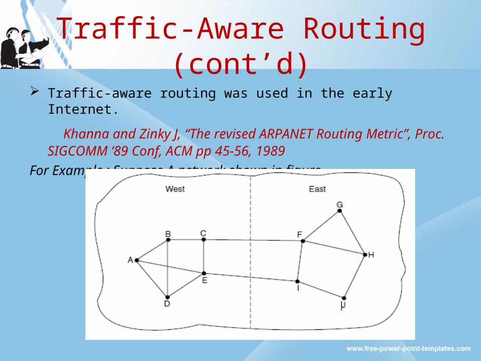
Traffic-Aware Routing (cont’d) Traffic-aware routing was used in the early Internet.

Khanna and Zinky J, “The revised ARPANET Routing Metric”, Proc. SIGCOMM ‘89 Conf, ACM pp 45-56, 1989

For Example : Suppose A network shown in figure

Traffic-Aware Routing (cont’d)

To avoid routing oscillation: Two technique can contribute to successful solution.

1. The first is multipath routing, in which there can be multiple paths from a source to a destination. In our example this means that the traffic can be spread across both of the East to West links.

2. The second one is for the routing scheme to shift traffic across routes slowly enough that it is able to converge.

Given these difficulties, in the Internet routing protocols do not generally adjust their routes depending on the load. Instead, adjustments are made outside the routing protocol by slowly changing its inputs. This is called traffic engineering.

Admission Control

One technique that is widely used in virtual-circuit networks to keep congestion at bay is admission control.

The idea is simple: do not set up a new virtual circuit unless the network can carry the added traffic without becoming congested.

Thus, attempts to set up a virtual circuit may fail. This is better than the alternative, as letting more people in when the network is busy just makes matters worse.

By analogy, in the telephone system, when a switch gets overloaded it practices admission control by not giving dial tones.

Admission Control (cont’d)

The task is straightforward in the telephone network because of the fixed bandwidth of calls (64 kbps for uncompressed audio).

virtual circuits in computer networks come in all shapes and sizes.

Thus, the circuit must come with some characterization of its traffic if we are to apply admission control.

Admission Control (cont’d)(Traffic Descriptor)

Traffic is often described in terms of its rate and shape. The main focus of congestion control and quality of service is The main focus of congestion control and quality of service is data trafficdata traffic. .

In congestion control we try to avoid traffic congestion. In congestion control we try to avoid traffic congestion. In quality of service, we try to create an appropriate environment for the In quality of service, we try to create an appropriate environment for the

traffic. traffic.

So, before talking about more details, we discuss the data traffic itself.So, before talking about more details, we discuss the data traffic itself.

Ref :Forouzan/ DCN/ Ch-24

Traffic descriptors

Ref :Forouzan/ DCN/ Ch-24

Three traffic profiles


The problem of how to describe it in a simple yet meaningful way is difficult because traffic is typically bursty—the average rate is only half the story.

For example: traffic that varies while browsing the Web is more difficult to handle than a streaming movie with the same long-term throughput because the bursts of Web traffic are more likely to congest routers in the network.

A commonly used descriptor that captures this effect is the leaky bucket or token bucket.


Armed with traffic descriptions, the network can decide whether to admit the new virtual circuit.

One possibility is for the network to reserve enough capacity along the paths of each of its virtual circuits that congestion will not occur.

In this case, the traffic description is a service agreement for what the network will guarantee its users.

Even without making guarantees, the network can use traffic descriptions for admission control.

The task is then to estimate how many circuits will fit within the carrying capacity of the network without congestion.

(But this task becomes bit tricky , as explained in example next slide)


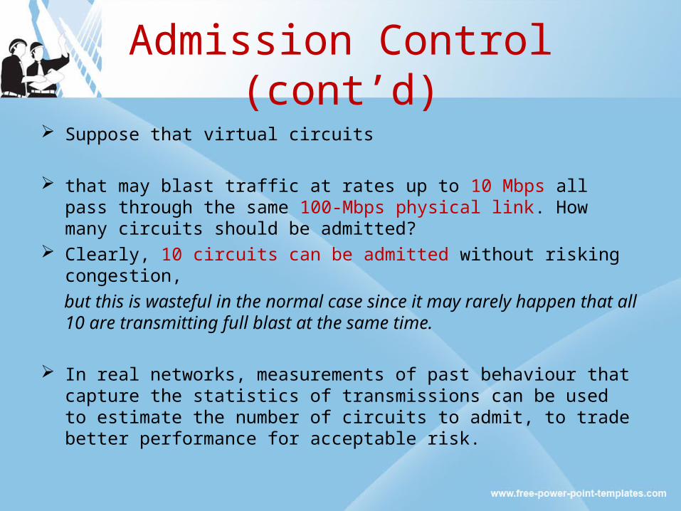
Suppose that virtual circuits

that may blast traffic at rates up to 10 Mbps all pass through the same 100-Mbps physical link. How many circuits should be admitted?

Clearly, 10 circuits can be admitted without risking congestion,

but this is wasteful in the normal case since it may rarely happen that all 10 are transmitting full blast at the same time.

In real networks, measurements of past behaviour that capture the statistics of transmissions can be used to estimate the number of circuits to admit, to trade better performance for acceptable risk.


Admission control can also be combined with traffic-aware routing by considering routes around traffic hotspots as part of the setup procedure. For Example :

Leaky Bucket

Used in conjunction with resource reservation to police the host’s reservation

At the host-network interface, allow packets into the network at a constant rate

Packets may be generated in a bursty manner, but after they pass through the leaky bucket, they enter the network evenly spaced

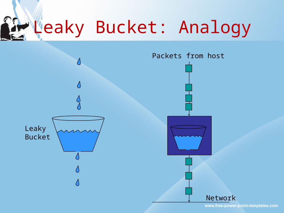
Leaky Bucket: Analogy

LeakyBucket

Network

Packets from host

Leaky Bucket (cont’d)

The leaky bucket is a “traffic shaper”: It changes the characteristics of packet stream

Traffic shaping makes more manageable and more predictable

Usually the network tells the leaky bucket the rate at which it may send packets when the connection begins

Leaky Bucket: Doesn’t allow bursty transmissions

• In some cases, we may want to allow short bursts of packets to enter the network without smoothing them out

• For this purpose we use a token bucket, which is a modified leaky bucket

Token Bucket

The bucket holds tokens instead of packets Tokens are generated and placed into the token bucket at

a constant rate When a packet arrives at the token bucket, it is

transmitted if there is a token available. Otherwise it is buffered until a token becomes available.

The token bucket has a fixed size, so when it becomes full, subsequently generated tokens are discarded

Token Bucket

Network

Packets from host

Token Generator(Generates a tokenonce every T seconds)

Token Bucket vs. Leaky Bucket

Case 1: Short burst arrivals

6543210

Arrival time at bucket

Departure time from a leaky bucketLeaky bucket rate = 1 packet / 2 time unitsLeaky bucket size = 4 packets

6543210

6543210

Departure time from a token bucketToken bucket rate = 1 tokens / 2 time unitsToken bucket size = 2 tokens

Token Bucket vs. Leaky Bucket

Case 2: Large burst arrivals

6543210

Arrival time at bucket

Departure time from a leaky bucketLeaky bucket rate = 1 packet / 2 time unitsLeaky bucket size = 2 packets

6543210

6543210

Departure time from a token bucketToken bucket rate = 1 token / 2 time unitsToken bucket size = 2 tokens

Contents

Traffic Throttling Choke PacketsExplicit Congestion Notification (ECN)Hope-by-Hope Backpressure

Traffic Throttling

In the Internet and many other computer networks, senders adjust their transmissions to send as much traffic as the network can readily deliver.

In this setting, the network aims to operate just before the onset of congestion.

When congestion is imminent, it must tell the senders to throttle back their transmissions and slow down.

There are some approaches to throttling traffic that can be used in both datagram networks and virtual-circuit networks.

Traffic Throttling (cont’d)

Each approach must solve two problems. First, routers must determine when congestion is

approaching, ideally before it has arrived. To do so, each router can continuously

monitor the resources it is using. Three possibilities are: the utilization of the

output links, the buffering of queued packets inside the router, and the number of packets that are lost due to insufficient buffering.


The second one is the most useful. Averages of utilization do not directly account for

the burstiness of most traffic—a utilization of 50% may be low for smooth traffic and too high for highly variable traffic.

The queueing delay inside routers directly captures any congestion experienced by packets.


To maintain a good estimate of the queueing delay d, a sample of the instantaneous queue length s, can be made periodically and d updated according to

dnew = αdold + (1 − α)s

where the constant α determines how fast the router forgets recent history. This is called an EWMA (Exponentially Weighted Moving Average).It smoothes out fluctuations and is equivalent to a low-pass filter. Whenever d moves above the threshold, the router notes the onset of congestion.


The second problem is that routers must deliver timely feedback to the senders that are causing the congestion.

To deliver feedback, the router must identify the appropriate senders. It must then warn them carefully, without sending many more packets into the already congested network.

Different schemes use different feedback mechanisms , Like

• Choke Packets• Explicit Congestion Notification• Hope-by-Hope Backpressure

Choke Packets Approach

The most direct way to notify a sender of congestion is to tell it directly.

In this approach, the router selects a congested packet and sends a choke packet back to the source host, giving it the destination found in the packet.

The original packet may be tagged (a header bit is turned on) so that it will not generate any more choke packets further along the path and then forwarded in the usual way.

To avoid increasing load on the network during a time of congestion, the router may only send choke packets at a low rate.

Forouzan/DCN/ CH.24

Choke packet

Choke Packets Approach

When the source host gets the choke packet, it is required to reduce the traffic sent to the specified destination, for example, by 50%.

For the same reason, it is likely that multiple choke packets will be sent to a given host and destination.

The host should ignore these additional chokes for the fixed time interval until its reduction in traffic takes effect. After that period, further choke packets indicate that the network is still congested.

The modern Internet uses an alternative notification design (Explicit congestion notification).

Explicit Congestion Notification

Instead of generating additional packets to warn of congestion, a router can tag any packet it forwards (by setting a bit in the packet’s header) to signal that it is experiencing congestion.

When the network delivers the packet, the destination can note that there is congestion and inform the sender when it sends a reply packet.

The sender can then throttle its transmissions as before.

This design is called ECN (Explicit Congestion Notification) and is used in the Internet.

Explicit Congestion Notification (cont’d)

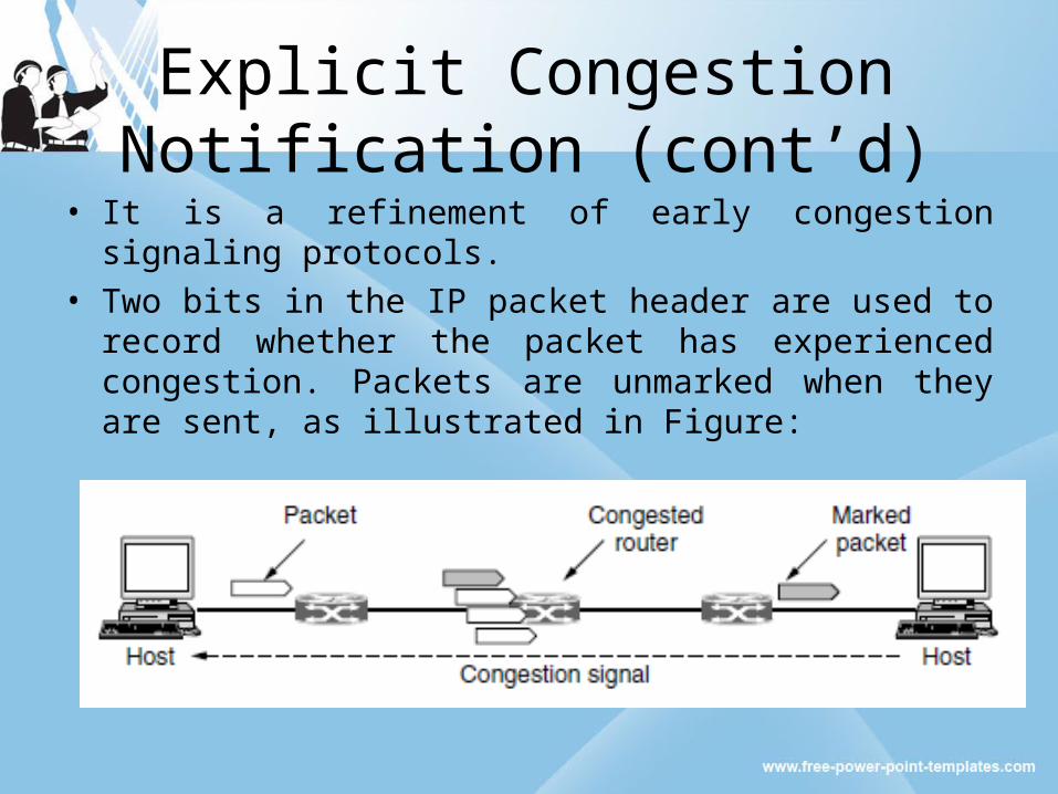
• It is a refinement of early congestion signaling protocols.

• Two bits in the IP packet header are used to record whether the packet has experienced congestion. Packets are unmarked when they are sent, as illustrated in Figure:

Explicit Congestion Notification (cont’d)

If any of the routers they pass through is congested, that router will then mark the packet as having experienced congestion as it is forwarded.

The destination will then echo any marks back to the sender as an explicit congestion signal in its next reply packet.

This is shown with a dashed line in the figure to indicate that it happens above the IP level (e.g., in TCP). The sender must then throttle its transmissions, as in the case of choke packets.

Forouzan/DCN/ Ch.24

Backpressure method for alleviating congestion

Hop-by-Hop Backpressure

At high speeds or over long distances, many new packets may be transmitted after congestion has been signalled because of the delay before the signal takes effect.

Consider, for example, a host in San Francisco (router A in Figure) that is sending traffic to a host in New York (router D in Figure) at the OC-3 speed of 155 Mbps.

If the New York host begins to run out of buffers, it will take about 40 msec for a choke packet to get back to San Francisco to tell it to slow down.

An ECN indication will take even longer because it is delivered via the destination.

• Choke packets:– Example showing

slow reaction– Solution: Hop-by-

Hop choke packets

• Hop-by-Hop choke packets– Have choke packet

take effect at every hop

– Problem: more buffers needed in routers

Hop-by-Hop Backpressure Choke packet propagation is illustrated as the second, third, and

fourth steps in figure. In those 40 msec, another 6.2 megabits will have been sent. Even

if

the host in San Francisco completely shuts down immediately, the 6.2 megabits in the pipe will continue to pour in and have to be dealt with.

Only in the seventh diagram in Fig. (a) will the New York router notice a slower flow.

An alternative approach is to have the choke packet take effect at every hop it passes through, as shown in the sequence of Fig. (b).

Here, as soon as the choke packet reaches F, F is required to reduce the flow to D. Doing so will require F to devote more buffers to the connection, since the source is still sending away at full blast, but it gives D immediate relief, like a headache remedy in a television commercial.

Hop-by-Hop Backpressure

In the next step, the choke packet reaches E, which tells E to reduce the flow to F. This action puts a greater demand on E’s buffers but

gives F immediate relief. Finally, the choke packet reaches A and the flow genuinely slows down.

The net effect of this hop-by-hop scheme is to provide quick relief at the point of congestion, at the price of using up more buffers upstream.

In this way, congestion can be nipped in the bud without losing any packets. The idea is discussed in detail by Mishra et al. (1996).

Load Shedding

When a router becomes inundated with packets, it simply drops some

Load Shedding

Load Shedding (Cont’d)

When none of the above methods make the congestion disappear, routers can bring out the heavy artillery: load shedding. Load shedding is a fancy way of saying that when routers are being inundated by packets that they cannot handle , they just throw them away.

The term comes from the world of electrical power generation, where it refers to the practice of utilities intentionally blacking out

certain areas to save the entire grid from collapsing on hot summer days when the demand for electricity greatly exceeds the supply.

The key question for a router drowning in packets is which packets to drop ?.


• The preferred choice may depend on the type of applications that use the network. For a file transfer, an old packet is worth more than a new one.

• In contrast, for real-time media, a new packet is worth more than an old one. This is because packets become useless if they are delayed and miss the time at which they must be played out to the user.

• The former policy (old is better than new) is often called wine and the latter (new is better than old) is often called milk because most people would rather drink new milk and old wine than the alternative.


An examples: packets that carry routing information. These packets are more important than regular data packets because they establish routes; if they are lost, the network may lose connectivity.

Another example is that algorithms for compressing video, like MPEG, periodically transmit an entire frame and then send subsequent frames as differences from the last full frame.

In this case, dropping a packet that is part of a difference is preferable to dropping one that is part of a full frame because future packets depend on the full frame


• More intelligent load shedding requires cooperation from the senders.

• To implement an intelligent discard policy, when packets have to be discarded, routers can first drop packets from the least

important class, then the next important class, and so on.• Unless there is some significant instruction to avoid marking every packet as VERY IMPORTANT—NEVER, EVER DISCARD, nobody

will do it.• For example,

• the network might let senders send faster than the service they purchased allows if they mark excess packets as low priority. Such a strategy is actually not a bad idea because it makes more efficient use of idle resources, allowing hosts to use them as long as nobody else is interested, but without establishing a right to

them when times get tough.

Intelligent Load Shedding

Discarding packets does not need to be done randomly Router should take other information into account Possibilities:

Total packet dropping Priority discarding Age biased discarding

Total Packet Dropping When the buffer fills and a packet segment is dropped, drop all the rest of

the segments from that packet, since they will be useless anyway Only works with routers that segment and reassemble packets

Priority Discarding Sources specify the priority of their packets When a packet is discarded, the router chooses a low priority packet Requires hosts to participate by labeling their packets with priority levels.

Age Biased Discarding When the router has to discard a packet, it chooses the oldest one in its

buffer This works well for multimedia traffic which requires short delays This may not work so well for data traffic, since more packets will need to be

retransmitted


Random Early Detection

Dealing with congestion when it first starts is more effective than letting it gum up the works and then trying to deal with it.

This observation leads to an interesting twist on load shedding, which is to discard packets before all the buffer

space is really exhausted. The motivation for this idea is that most Internet hosts do

not yet get congestion signals from routers in the form of ECN.

Instead, the only reliable indication of congestion that hosts get from the network is packet loss.

After all, it is difficult to build a router that does not drop packets when it is overloaded.


Transport protocols such as TCP are thus hardwired to react to loss as congestion, slowing down the source in response.

The reasoning behind this logic is that TCP was designed for wired networks and wired networks are very reliable, so lost packets are mostly due to buffer overruns rather than transmission errors

. Wireless links must recover transmission errors at the link

layer (so they are not seen at the network layer) to work well with TCP.

This situation can be exploited to help reduce congestion. By having routers drop packets early, before the situation has become hopeless, there is time for the source to take action before it is too late


A popular algorithm for doing this is called RED (Random Early Detection) (Floyd and Jacobson, 1993).

To determine when to start discarding, routers maintain a running average of their queue lengths.

When the average queue length on some link exceeds a threshold, the link is said to be congested and a small fraction of the packets are dropped at random.

Picking packets at random makes it more likely that the fastest senders will see a packet drop; this is the best option since the router cannot tell which source is causing the most trouble in a datagram network.


• The affected sender will notice the loss when there is no acknowledgement, and then the transport protocol will slow down.

• The lost packet is thus delivering the same message as a choke packet, but implicitly, without the router sending any explicit

signal.• RED routers improve performance compared to routers that drop

packets only when their buffers are full, though they may require tuning to work well.

• For example, the number of packets to drop depends on how many senders need to be notified of congestion.

• However, ECN is the preferred option if it is available . It works in exactly the same manner, but delivers a congestion signal explicitly

rather than as a loss; RED is used when hosts cannot receive explicit signals.

Jitter Control

In real-time interactive audio/video, people communicate with one another in real time.

The Internet phone or voice over IP is an example of this type of application.

Video conferencing is another example that allows people to communicate visually and orally.

Jitter Control(Cont’d)

Time Relationship: Real-time data on a packet-switched network require the

preservation of the time relationship between packets of a session.

For example, let us assume that a real-time video server creates live video images and sends them online.

The video is digitized and packetized. There are only three packets, and each packet holds 10s of

video information.


The first packet starts at 00:00:00, the second packet starts at 00:00: 10, and the

third packet starts at 00:00:20. Also imagine that it takes 1 s for each packet to reach the

destination (equal delay). The receiver can play back the first packet at 00:00:01, the

second packet at 00:00:11, and the third packet at 00:00:21.


Figure: Time relationship


But what happens if the packets arrive with different delays? For example, say the first packet arrives at 00:00:01 (1-s delay), the second arrives at 00:00: 15 (5-s delay), and the third arrives at 00:00:27 (7-s delay). If the receiver starts playing the first packet at 00:00:01, it will finish at 00:00: 11. However, the next packet has not yet arrived; itarrives 4 s later.


•There is a gap between the first and second packets and between the second and the third as the video is viewed at the remote site. • This phenomenon is called jitter. • Jitter is introduced in real-time data by the delay between packets.

Jitter Control(Cont’d)Timestamp:• One solution to jitter is the use of a timestamp. • If each packet has a timestamp that shows the time it was produced relative to the first (or previous) packet, then the receiver can add this time to the time at which it starts the playback. • In other words, the receiver knows when each packet is to be played.

Jitter Control(Cont’d)•Imagine the first packet in the previous examplehas a timestamp of 0, the second has a timestamp of 10, and the third has a timestamp of20. • If the receiver starts playing back the first packet at 00:00:08, the second will be played at 00:00: 18 and the third at 00:00:28. • There are no gaps between the packets.• Next Figure shows the situation.


Figure: Timestamp• To prevent jitter, we can time-stamp the packets and separate the arrival time from the playback time.

Playback Buffer: To be able to separate the arrival time from the playback time, we need a buffer to storethe data until they are played back. The buffer is referred to as a playback buffer. When a session begins (the first bit of the first packet arrives), the receiver delays playing the data until a threshold is reached. In the previous example, the first bit of the first packet arrives at 00:00:01; the threshold is 7 s, and the playback time is 00:00:08.


• The threshold is measured in time units of data. The replay does not start until the time unitsof data are equal to the threshold value.• Data are stored in the buffer at a possibly variable rate, but they are extracted and played back at a fixed rate.• Next Figure shows the buffer at different times for our example.

Figure: Playback buffer

• A playback buffer is required for real-time traffic.

Other Characteristics

• Ordering

• Multicasting

• Translation

• Mixing

EXAMPLES

To better understand the concept of congestion control, To better understand the concept of congestion control, let us give an example: let us give an example:

Congestion Control in TCP

Slow start, exponential increase

In the slow-start algorithm, the size of the congestion window increases exponentially until it reaches a threshold.

Note

Figure 24.9 Congestion avoidance, additive increase

In the congestion avoidance algorithm, the size of the congestion window increases additively until congestion is detected.

Note

An implementation reacts to congestion detection in one of the following ways:❏ If detection is by time-out, a new slow start phase starts.❏ If detection is by three ACKs, a new congestion avoidance phase starts.

Congestion example

References

1. Andrew S. Tanenbaum, Devid J. Wetherall, “ Computer Networks” , Pearson , 5th Edition

2. Andrew S. Tanenbaum, Devid J. Wetherall, “ Computer Networks” , Pearson , 3rd Edition

3. Behrouz A Forouzan”Data Communications and Networking” TMH,4th Edition.

4. http://tools.ietf.org/html/rfc2581 [RFC 2581]

5. http://www.rfc-base.org/rfc-5681.html [RFC 5681]

6. www.net-seal.net

http://tools.ietf.org/html/rfc2581

http://www.rfc-base.org/rfc-5681.html

http://www.net-seal.net/






congetion control.pptx

Engineering

congestion control algorithms

presence of congestion

major cause of congestion

growing congestion pass

congestin control

open loop control

new born congestion

control theory viewpoint