common functional principal componentst1
TRANSCRIPT

The Annals of Statistics2009, Vol. 37, No. 1, 1–34DOI: 10.1214/07-AOS516© Institute of Mathematical Statistics, 2009
COMMON FUNCTIONAL PRINCIPAL COMPONENTS1
BY MICHAL BENKO, WOLFGANG HÄRDLE AND ALOIS KNEIP
Humboldt-Universität, Humboldt-Universität and Bonn Universität
Functional principal component analysis (FPCA) based on the Karhunen–Loève decomposition has been successfully applied in many applications,mainly for one sample problems. In this paper we consider common func-tional principal components for two sample problems. Our research is mo-tivated not only by the theoretical challenge of this data situation, but alsoby the actual question of dynamics of implied volatility (IV) functions. Fordifferent maturities the log-returns of IVs are samples of (smooth) randomfunctions and the methods proposed here study the similarities of their sto-chastic behavior. First we present a new method for estimation of functionalprincipal components from discrete noisy data. Next we present the two sam-ple inference for FPCA and develop the two sample theory. We proposebootstrap tests for testing the equality of eigenvalues, eigenfunctions, andmean functions of two functional samples, illustrate the test-properties bysimulation study and apply the method to the IV analysis.
1. Introduction. In many applications in biometrics, chemometrics, econo-metrics, etc., the data come from the observation of continuous phenomenons oftime or space and can be assumed to represent a sample of i.i.d. smooth randomfunctions X1(t), . . . , Xn(t) ∈ L2[0,1]. Functional data analysis has received con-siderable attention in the statistical literature during the last decade. In this contextfunctional principal component analysis (FPCA) has proved to be a key technique.An early reference is Rao (1958), and important methodological contributions havebeen given by various authors. Case studies and references, as well as methodolog-ical and algorithmical details, can be found in the books by Ramsay and Silverman(2002, 2005) or Ferraty and Vieu (2006).
The well-known Karhunen–Loève (KL) expansion provides a basic tool to de-scribe the distribution of the random functions Xi and can be seen as the the-oretical basis of FPCA. For v,w ∈ L2[0,1], let 〈v,w〉 = ∫ 1
0 v(t)w(t) dt , and let‖ · ‖= 〈·, ·〉1/2 denote the usual L2-norm. With λ1 ≥ λ2 ≥ · · · and γ1, γ2, . . . denot-ing eigenvalues and corresponding orthonormal eigenfunctions of the covarianceoperator � of Xi , we obtain Xi = μ+∑∞
r=1 βriγr , i = 1, . . . , n, where μ = E(Xi)
Received January 2006; revised February 2007.1Supported by the Deutsche Forschungsgemeinschaft and the Sonderforschungsbereich 649
“Ökonomisches Risiko.”AMS 2000 subject classifications. Primary 62H25, 62G08; secondary 62P05.Key words and phrases. Functional principal components, nonparametric regression, bootstrap,
two sample problem.
1

2 M. BENKO, W. HÄRDLE AND A. KNEIP
is the mean function and βri = 〈Xi − μ,γr〉 are (scalar) factor loadings withE(β2
ri) = λr . Structure and dynamics of the random functions can be assessed byanalyzing the “functional principal components” γr , as well as the distribution ofthe factor loadings. For a given functional sample, the unknown characteristicsλr, γr are estimated by the eigenvalues and eigenfunctions of the empirical covari-ance operator �n of X1, . . . ,Xn. Note that an eigenfunction γr is identified (up tosign) only if the corresponding eigenvalue λr has multiplicity one. This thereforeestablishes a necessary regularity condition for any inference based on an esti-mated functional principal component γr in FPCA. Signs are arbitrary (γr and βri
can be replaced by −γr and −βri ) and may be fixed by a suitable standardization.More detailed discussion on this topic and precise assumptions can be found inSection 2.
In many important applications a small number of functional principal compo-nents will suffice to approximate the functions Xi with a high degree of accuracy.Indeed, FPCA plays a much more central role in functional data analysis than itswell-known analogue in multivariate analysis. There are two major reasons. First,distributions on function spaces are complex objects, and the Karhunen–Loève ex-pansion seems to be the only practically feasible way to access their structure. Sec-ond, in multivariate analysis a substantial interpretation of principal components isoften difficult and has to be based on vague arguments concerning the correlationof principal components with original variables. Such a problem does not at allexists in the functional context, where γ1(t), γ2(t), . . . are functions representingthe major modes of variation of Xi(t) over t .
In this paper we consider inference and tests of hypotheses on the structure offunctional principal components. Motivated by an application to implied volatilityanalysis, we will concentrate on the two sample case. A central point is the useof bootstrap procedures. We will show that the bootstrap methodology can also beapplied to functional data.
In Section 2 we start by discussing one-sample inference for FPCA. Basic re-sults on asymptotic distributions have already been derived by Dauxois, Pousseand Romain (1982) in situations where the functions are directly observable. Halland Hosseini-Nasab (2006) develop asymptotic Taylor expansions of estimatedeigenfunctions in terms of the difference �n − �. Without deriving rigorous theo-retical results, they also provide some qualitative arguments as well as simulationresults motivating the use of bootstrap in order to construct confidence regions forprincipal components.
In practice, the functions of interest are often not directly observed, but are re-gression curves which have to be reconstructed from discrete, noisy data. In thiscontext the standard approach is to first estimate individual functions nonpara-metrically (e.g., by B-splines) and then to determine principal components of theresulting estimated empirical covariance operator—see Besse and Ramsay (1986),Ramsay and Dalzell (1991), among others. Approaches incorporating a smooth-ing step into the eigenanalysis have been proposed by Rice and Silverman (1991),
COMMON FUNCTIONAL PC 3
Pezzulli and Silverman (1993) or Silverman (1996). Robust estimation of princi-pal components has been considered by Lacontore et al. (1999). Yao, Müller andWang (2005) and Hall, Müller and Wang (2006) propose techniques based on non-parametric estimation of the covariance function E[{Xi(t) − μ(t)}{Xi(s) − μ(s)}]which can also be applied if there are only a few scattered observations per curve.
Section 2.1 presents a new method for estimation of functional principal com-ponents. It consists in an adaptation of a technique introduced by Kneip and Utikal(2001) for the case of density functions. The key-idea is to represent the compo-nents of the Karhunen–Loève expansion in terms of an (L2) scalar-product matrixof the sample. We investigate the asymptotic properties of the proposed method.It is shown that under mild conditions the additional error caused by estimationfrom discrete, noisy data is first-order asymptotically negligible, and inference mayproceed “as if” the functions were directly observed. Generalizing the results ofDauxois, Pousse and Romain (1982), we then present a theorem on the asymptoticdistributions of the empirical eigenvalues and eigenfunctions. The structure of theasymptotic expansion derived in the theorem provides a basis to show consistencyof bootstrap procedures.
Section 3 deals with two-sample inference. We consider two independent sam-ples of functions {X(1)
i }n1i=1 and {X(2)
i }n2i=1. The problem of interest is to test in how
far the distributions of these random functions coincide. The structure of the dif-ferent distributions in function space can be accessed by means of the respectiveKarhunen–Loève expansions
X(p)i = μ(p) +
∞∑r=1
β(p)ri γ (p)
r , p = 1,2.
Differences in the distribution of these random functions will correspond to dif-ferences in the components of the respective KL expansions above. Without re-striction, one may require that signs are such that 〈γ (1)
r , γ(2)r 〉 ≥ 0. Two sample
inference for FPCA in general has not been considered in the literature so far. InSection 3 we define bootstrap procedures for testing the equality of mean func-tions, eigenvalues, eigenfunctions and eigenspaces. Consistency of the bootstrapis derived in Section 3.1, while Section 3.2 contains a simulation study providinginsight into the finite sample performance of our tests.
It is of particular interest to compare the functional components characterizingthe two samples. If these factors are “common,” this means γr := γ
(1)r = γ
(2)r , then
only the factor loadings β(p)ri may vary across samples. This situation may be seen
as a functional generalization of the concept of “common principal components”as introduced by Flury (1988) in multivariate analysis. A weaker hypothesis mayonly require equality of the eigenspaces spanned by the first L ∈ N functional prin-cipal components. [N denotes the set of all natural numbers 1,2, . . . (0 /∈ N)]. If forboth samples the common L-dimensional eigenspaces suffice to approximate the

4 M. BENKO, W. HÄRDLE AND A. KNEIP
functions with high accuracy, then the distributions in function space are well rep-resented by a low-dimensional factor model, and subsequent analysis may rely oncomparing the multivariate distributions of the random vectors (β
(p)r1 , . . . , β
(p)rL )�.
The idea of “common functional principal components” is of considerable im-portance in implied volatility (IV) dynamics. This application is discussed in de-tail in Section 4. Implied volatility is obtained from the pricing model proposedby Black and Scholes (1973) and is a key parameter for quoting options prices.Our aim is to construct low-dimensional factor models for the log-returns ofthe IV functions of options with different maturities. In our application the firstgroup of functional observations—{X(1)
i }n1i=1, are log-returns on the maturity “1
month” (1M group) and second group—{X(2)i }n2
i=1, are log-returns on the maturity“3 months” (3M group).
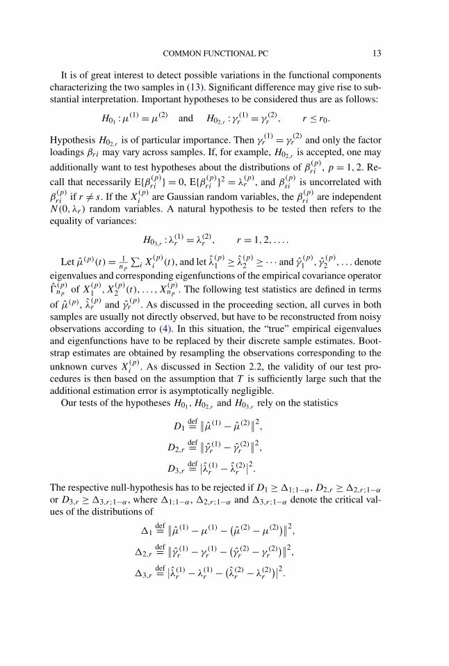
The first three eigenfunctions (ordered with respect to the corresponding eigen-values), estimated by the method described in Section 2.1, are plotted in Figure 1.The estimated eigenfunctions for both groups are of similar structure, which mo-tivates a common FPCA approach. Based on discretized vectors of functional val-ues, a (multivariate) common principal components analysis of implied volatilitieshas already been considered by Fengler, Härdle and Villa (2003). They rely onthe methodology introduced by Flury (1988) which is based on maximum like-lihood estimation under the assumption of multivariate normality. Our analysisovercomes the limitations of this approach by providing specific hypothesis testsin a fully functional setup. It will be shown in Section 4 that for both groups L = 3components suffice to explain 98.2% of the variability of the sample functions. Anapplication of the tests developed in Section 3 does not reject the equality of thecorresponding eigenspaces.
FIG. 1. Estimated eigenfunctions for 1M group in the left plot and 3M group in the right plot:solid—first function, dashed—second function, finely dashed—third function.

COMMON FUNCTIONAL PC 5
2. Functional principal components and one sample inference. In this sec-tion we will focus on one sample of i.i.d. smooth random functions X1, . . . ,Xn ∈L2[0,1]. We will assume a well-defined mean function μ = E(Xi), as well as theexistence of a continuous covariance function σ(t, s) = E[{Xi(t) − μ(t)}{Xi(s) −μ(s)}]. Then E(‖Xi − μ‖2) = ∫
σ(t, t) dt < ∞, and the covariance operator � ofXi is given by
(�v)(t) =∫
σ(t, s)v(s) ds, v ∈ L2[0,1].The Karhunen–Loève decomposition provides a basic tool to describe the dis-
tribution of the random functions Xi . With λ1 ≥ λ2 ≥ · · · and γ1, γ2, . . . denotingeigenvalues and a corresponding complete orthonormal basis of eigenfunctions of�, we obtain
Xi = μ +∞∑
r=1
βriγr , i = 1, . . . , n,(1)
where βri = 〈Xi −μ,γr〉 are uncorrelated (scalar) factor loadings with E(βri) = 0,E(β2
ri) = λr and E(βriβki) = 0 for r = k. Structure and dynamics of the randomfunctions can be assessed by analyzing the “functional principal components” γr ,as well as the distribution of the factor loadings.
A discussion of basic properties of (1) can, for example, be found in Gihman andSkorohod (1973). Under our assumptions, the infinite sums in (1) converge withprobability 1, and
∑∞r=1 λr = E(‖Xi − μ‖2) < ∞. Smoothness of Xi carries over
to a corresponding degree of smoothness of σ(t, s) and γr . If, with probability 1,Xi(t) is twice continuously differentiable, then σ as well as γr are also twicecontinuously differentiable. The particular case of a Gaussian random function Xi
implies that the βri are independent N(0, λr)-distributed random variables.An important property of (1) consists in the known fact that the first L principal
components provide a “best basis” for approximating the sample functions in termsof the integrated square error; see Ramsay and Silverman (2005), Section 6.2.3,among others. For any choice of L orthonormal basis functions v1, . . . , vL, themean integrated square error
ρ(v1, . . . , vL) = E
(∥∥∥∥∥Xi − μ −L∑
r=1
〈Xi − μ,vr〉vr
∥∥∥∥∥2)
(2)
is minimized by vr = γr .
2.1. Estimation of functional principal components. For a given sample anempirical analog of (1) can be constructed by using eigenvalues λ1 ≥ λ2 ≥ · · · andorthonormal eigenfunctions γ1, γ2, . . . of the empirical covariance operator �n,where
(�nv)(t) =∫
σ (t, s)v(s) ds,

6 M. BENKO, W. HÄRDLE AND A. KNEIP
with X = n−1∑ni=1 Xi and σ (t, s) = n−1∑n
i=1{Xi(t) − X(t)}{Xi(s) − X(s)} de-noting sample mean and covariance function. Then
Xi = X +n∑
r=1
βri γr , i = 1, . . . , n,(3)
where βri = 〈γr ,Xi − X〉. We necessarily obtain n−1∑i βri = 0, n−1∑
i βri βsi =0 for r = s, and n−1∑
i β2ri = λr .
Analysis will have to concentrate on the leading principal components ex-plaining the major part of the variance. In the following we will assume thatλ1 > λ2 > · · · > λr0 > λr0+1, where r0 denotes the maximal number of compo-nents to be considered. For all r = 1, . . . , r0, the corresponding eigenfunction γr
is then uniquely defined up to sign. Signs are arbitrary, decompositions (1) or (3)may just as well be written in terms of −γr,−βri or −γr ,−βri , and any suitablestandardization may be applied by the statistician. In order to ensure that γr maybe viewed as an estimator of γr rather than of −γr , we will in the following onlyassume that signs are such that 〈γr, γr〉 ≥ 0. More generally, any subsequent state-ment concerning differences of two eigenfunctions will be based on the conditionof a nonnegative inner product. This does not impose any restriction and will gowithout saying.
The results of Dauxois, Pousse and Romain (1982) imply that, under regularityconditions, ‖γr −γr‖ = Op(n−1/2), |λr −λr | = Op(n−1/2), as well as |βri −βri | =Op(n−1/2) for all r ≤ r0.
However, in practice, the sample functions Xi are often not directly observed,but have to be reconstructed from noisy observations Yij at discrete design pointstik :
Yik = Xi(tik) + εik, k = 1, . . . , Ti,(4)
where εik are independent noise terms with E(εik) = 0, Var(εik) = σ 2i .
Our approach for estimating principal components is motivated by the well-known duality relation between row and column spaces of a data matrix; seeHärdle and Simar (2003), Chapter 8, among others. In a first step this approachrelies on estimating the elements of the matrix:
Mlk = 〈Xl − X,Xk − X〉, l, k = 1, . . . , n.(5)
Some simple linear algebra shows that all nonzero eigenvalues λ1 ≥ λ2 · · · of �n
and l1 ≥ l2 · · · of M are related by λr = lr/n, r = 1,2, . . . . When using the corre-sponding orthonormal eigenvectors p1,p2, . . . of M , the empirical scores βri , aswell as the empirical eigenfunctions γr , are obtained by βri = √
lrpir and
γr = 1√lr
n∑i=1
pir(Xi − X) = 1√lr
n∑i=1
pirXi.(6)

COMMON FUNCTIONAL PC 7
The elements of M are functionals which can be estimated with asympoticallynegligible bias and a parametric rate of convergence T
−1/2i . If the data in (4) is
generated from a balanced, equidistant design, then it is easily seen that for i = j
this rate of convergence is achieved by the estimator
Mij = T −1T∑
k=1
(Yik − Y·k)(Yjk − Y·k), i = j,
and
Mii = T −1T∑
k=1
(Yik − Y·k)2 − σ 2i ,
where σ 2i denotes some nonparametric estimator of variance and Y·k = n−1 ×∑n
j=1 Yjk .In the case of a random design some adjustment is necessary: Define the ordered
sample ti(1) ≤ ti(2) ≤ · · · ≤ ti(Ti) of design points, and for j = 1, . . . , Ti , let Yi(j)
denote the observation belonging to ti(j). With ti(0) = −ti(1) and ti(Ti+1) = 2 −ti(Ti), set
χi(t) =Ti∑
j=1
Yi(j)I
(t ∈[ti(j−1) + ti(j)
2,ti(j) + ti(j+1)
2
)), t ∈ [0,1],
where I (·) denotes the indicator function, and for i = j , define the estimate of Mij
by
Mij =∫ 1
0{χi(t) − χ(t)}{χj (t) − χ (t)}dt,
where χ(t) = n−1∑ni=1 χi(t). Finally, by redefining ti(1) = −ti(2) and ti(Ti+1) =
2 − ti(Ti), set χ∗i (t) =∑Ti
j=2 Yi(j−1)I (t ∈ [ ti(j−1)+ti(j)
2 ,ti(j)+ti(j+1)
2 )), t ∈ [0,1]. Thenconstruct estimators of the diagonal terms Mii by
Mii =∫ 1
0{χi(t) − χ (t)}{χ∗
i (t) − χ (t)}dt.(7)
The aim of using the estimator (7) for the diagonal terms is to avoid the additionalbias implied by Eε(Y
2ik) = Xi(tij )
2 + σ 2i . Here Eε denotes conditional expecta-
tion given tij , Xi . Alternatively, we can construct a bias corrected estimator usingsome nonparametric estimation of variance σ 2
i , for example, the difference basedmodel-free variance estimators studied in Hall, Kay and Titterington (1990) canbe employed.
The eigenvalues l1 ≥ l2 · · · and eigenvectors p1, p2, . . . of the resulting matrix
M then provide estimates λr;T = lr /n and βri;T =√
lr pir of λr and βri . Esti-mates γr;T of the empirical functional principal component γr can be determined
8 M. BENKO, W. HÄRDLE AND A. KNEIP
from (6) when replacing the unknown true functions Xi by nonparametric esti-mates Xi (as, for example, local polynomial estimates) with smoothing parameter(bandwidth) b:
γr;T = 1√lr
n∑i=1
pir Xi .(8)
When considering (8), it is important to note that γr;T is defined as a weightedaverage of all estimated sample functions. Averaging reduces variance, and ef-ficient estimation of γr therefore requires undersmoothing of individual functionestimates Xi . Theoretical results are given in Theorem 1 below. Indeed, if, forexample, n and T = mini Ti are of the same order of magnitude, then under suit-able additional regularity conditions it will be shown that for an optimal choiceof a smoothing parameter b ∼ (nT )−1/5 and twice continuously differentiable Xi ,we obtain the rate of convergence ‖γr − γr;T ‖ = Op{(nT )−2/5}. Note, however,that the bias corrected estimator (7) may yield negative eigenvalues. In practice,these values will be small and will have to be interpreted as zero. Furthermore,the eigenfunctions determined by (8) may not be exactly orthogonal. Again, whenusing reasonable bandwidths, this effect will be small, but of course (8) may byfollowed by a suitable orthogonalization procedure.
It is of interest to compare our procedure to more standard methods for estimat-ing λr and γr as mentioned above. When evaluating eigenvalues and eigenfunc-tions of the empirical covariance operator of nonparametrically estimated curvesXi , then for fixed r ≤ r0 the above rate of convergence for the estimated eigenfunc-tions may well be achieved for a suitable choice of smoothing parameters (e.g.,number of basis functions). But as will be seen from Theorem 1, our approach
also implies that |λr − lrn| = Op(T −1 + n−1). When using standard methods it
does not seem to be possible to obtain a corresponding rate of convergence, sinceany smoothing bias |E[Xi(t)] − Xi(t)| will invariably affect the quality of the cor-responding estimate of λr .
We want to emphasize that any finite sample interpretation will require that T issufficiently large such that our nonparametric reconstructions of individual curvescan be assumed to possess a fairly small bias. The above arguments do not applyto extremely sparse designs with very few observations per curve [see Hall, Müllerand Wang (2006) for an FPCA methodology focusing on sparse data].
Note that, in addition to (8), our final estimate of the empirical mean functionμ = X will be given by μT = n−1∑
i Xi . A straightforward approach to determinea suitable bandwidth b consists in a “leave-one-individual-out” cross-validation.For the maximal number r0 of components to be considered, let μT ,−i and γr;T ,−i ,r = 1, . . . , r0, denote the estimates of μ and γr obtained from the data (Ylj , tlj ),l = 1, . . . , i − 1, i + 1, . . . , n, j = 1, . . . , Tk . By (8), these estimates depend on b,

COMMON FUNCTIONAL PC 9
and one may approximate an optimal smoothing parameter by minimizing
∑i
∑j
{Yij − μT ,−i (tij ) −
r0∑r=1
ϑri γr;T ,−i(tij )
}2
over b, where ϑri denote ordinary least squares estimates of βri . A more sophis-ticated version of this method may even allow to select different bandwidths br
when estimating different functional principal components by (8). Although, un-der certain regularity conditions, the same qualitative rates of convergence hold forany arbitrary fixed r ≤ r0, the quality of estimates decreases when r becomes large.Due to 〈γs, γr〉 = 0 for s < r , the number of zero crossings, peaks and valleys ofγr has to increase with r . Hence, in tendency γr will be less and less smooth as r
increases. At the same time, λr → 0, which means that for large r the r th eigen-functions will only possess a very small influence on the structure of Xi . This inturn means that the relative importance of the error terms εik in (4) on the structureof γr;T will increase with r .
2.2. One sample inference. Clearly, in the framework described by (1)–(4) weare faced with two sources of variability of estimated functional principal compo-nents. Due to sampling variation, γr will differ from the true component γr , anddue to (4), there will exist an additional estimation error when approximating γr
by γr;T .The following theorems quantify the order of magnitude of these different types
of error. Our theoretical results are based on the following assumptions on thestructure of the random functions Xi .
ASSUMPTION 1. X1, . . . ,Xn ∈ L2[0,1] is an i.i.d. sample of random func-tions with mean μ and continuous covariance function σ(t, s), and (1) holds fora system of eigenfunctions satisfying sups∈N supt∈[0,1] |γs(t)| < ∞. Furthermore,∑∞
r=1∑∞
s=1 E[β2riβ
2si] < ∞ and
∑∞q=1
∑∞s=1 E[β2
riβqiβsi] < ∞ for all r ∈ N.Recall that E[βri] = 0 and E[βriβsi] = 0 for r = s. Note that the assumption
on the factor loadings is necessarily fulfilled if Xi are Gaussian random functions.Then βri and βsi are independent for r = s, all moments of βri are finite, and henceE[β2
riβqiβsi] = 0 for q = s, as well as E[β2riβ
2si] = λrλs for r = s; see Gihman and
Skorohod (1973).
We need some further assumptions concerning smoothness of Xi and the struc-ture of the discrete model (4).
ASSUMPTION 2. (a) Xi is a.s. twice continuously differentiable. There existsa constant D1 < ∞ such that the derivatives are bounded by supt E[Xi
′(t)4] ≤ D1,as well as supt E[Xi
′′(t)4] ≤ D1.

10 M. BENKO, W. HÄRDLE AND A. KNEIP
(b) The design points tik , i = 1, . . . , n, k = 1, . . . , Ti , are i.i.d. random vari-ables which are independent of Xi and εik . The corresponding design density f iscontinuous on [0,1] and satisfies inft∈[0,1] f (t) > 0.
(c) For any i, the error terms εik are i.i.d. zero mean random variables withVar(εik) = σ 2
i . Furthermore, εik is independent of Xi , and there exists a constantD2 such that E(ε8
ik) < D2 for all i, k.(d) The estimates Xi used in (8) are determined by either a local linear or a
Nadaraya–Watson kernel estimator with smoothing parameter b and kernel func-tion K . K is a continuous probability density which is symmetric at 0.
The following theorems provide asymptotic results as n,T → ∞, where T =minn
i=1{Ti}.THEOREM 1. In addition to Assumptions 1 and 2, assume that infs =r |λr −
λs | > 0 holds for some r = 1,2, . . . . Then we have the following:
(i) n−1∑ni=1(βri − βri;T )2 = Op(T −1) and∣∣∣∣λr − lr
n
∣∣∣∣= Op(T −1 + n−1).(9)
(ii) If additionally b → 0 and (T b)−1 → 0 as n,T → ∞, then for all t ∈ [0,1],|γr (t) − γr;T (t)| = Op{b2 + (nT b)−1/2 + (T b1/2)−1 + n−1}.(10)
A proof is given in the Appendix.
THEOREM 2. Under Assumption 1 we obtain the following:
(i) For all t ∈ [0,1],√
n{X(t) − μ(t)} =∑r
{1√n
n∑i=1
βri
}γr(t)
L→ N
(0,∑r
λrγr(t)2
).
If, furthermore, λr−1 > λr > λr+1 holds for some fixed r ∈ {1,2, . . .}, then(ii)
√n(λr − λr) = 1√
n
n∑i=1
(β2ri − λr) + Op(n−1/2)
L→ N(0,�r),(11)
where �r = E[(β2ri − λr)
2],(iii) and for all t ∈ [0,1]
γr (t) − γr(t) =∑s =r
{1
n(λr − λs)
n∑i=1
βsiβri
}γs(t) + Rr(t),
(12)where ‖Rr‖ = Op(n−1).
COMMON FUNCTIONAL PC 11
Moreover,
√n∑s =r
{1
n(λr − λs)
n∑i=1
βsiβri
}γs(t)
L→ N
(0,∑q =r
∑s =r
E[β2riβqiβsi]
(λq − λr)(λs − λr)γq(t)γs(t)
).
A proof can be found in the Appendix. The theorem provides a generalization ofthe results of Dauxois, Pousse and Romain (1982) who derive explicit asymptoticdistributions by assuming Gaussian random functions Xi . Note that in this case
�r = 2λ2r and
∑q =r
∑s =r
E[β2riβqiβsi ]
(λq−λr )(λs−λr )γq(t)γs(t) =∑
s =rλrλs
(λs−λr )2 γs(t)2.
When evaluating the bandwidth-dependent terms in (10), best rates of conver-gence |γr (t)− γr;T (t)| = Op{(nT )−2/5 +T −4/5 +n−1} are achieved when choos-ing an undersmoothing bandwidth b ∼ max{(nT )−1/5, T −2/5}. Theoretical workin functional data analysis is usually based on the implicit assumption that theadditional error due to (4) is negligible, and that one can proceed “as if” the func-tions Xi were directly observed. In view of Theorems 1 and 2, this approach isjustified in the following situations:
(1) T is much larger than n, that is, n/T 4/5 → 0, and the smoothing parame-ter b in (8) is of order T −1/5 (optimal smoothing of individual functions).
(2) An undersmoothing bandwidth b ∼ max{(nT )−1/5, T −2/5} is used andn/T 8/5 → 0. This means that T may be smaller than n, but T must be at leastof order of magnitude larger than n5/8.
In both cases (1) and (2) the above theorems imply that |λr − lrn| = Op(|λr −
λr |), as well as ‖γr − γr;T ‖ = Op(‖γr − γr‖). Inference about functional principalcomponents will then be first-order equivalent to an inference based on knownfunctions Xi .
In such situations Theorem 2 suggests bootstrap procedures as tools for onesample inference. For example, the distribution of ‖γr −γr‖ may by approximatedby the bootstrap distribution of ‖γ ∗
r − γr‖, where γ ∗r are estimates to be obtained
from i.i.d. bootstrap resamples X∗1,X∗
2, . . . ,X∗n of {X1,X2, . . . ,Xn}. This means
that X∗1 = Xi1, . . . ,X
∗n = Xin for some indices i1, . . . , in drawn independently and
with replacement from {1, . . . , n} and, in practice, γ ∗r may thus be approximated
from corresponding discrete data (Yi1j , ti1j )j=1,...,Ti1, . . . , (Yinj , tinj )j=1,...,Tin
.The additional error is negligible if either (1) or (2) is satisfied.
One may wonder about the validity of such a bootstrap. Functions are com-plex objects and there is no established result in bootstrap theory which readilygeneralizes to samples of random functions. But by (1), i.i.d. bootstrap resam-ples {X∗
i }i=1,...,n may be equivalently represented by corresponding, i.i.d. resam-ples {β∗
1i , β∗2i , . . .}i=1,...,n of factor loadings. Standard multivariate bootstrap the-
12 M. BENKO, W. HÄRDLE AND A. KNEIP
orems imply that for any q ∈ N the distribution of moments of the random vec-tors (β1i , . . . , βqi) may be consistently approximated by the bootstrap distributionof corresponding moments of (β∗
1i , . . . , β∗qi). Together with some straightforward
limit arguments as q → ∞, the structure of the first-order terms in the asymptoticexpansions (11) and (12) then allows to establish consistency of the functionalbootstrap. These arguments will be made precise in the proof of Theorem 3 below,which concerns related bootstrap statistics in two sample problems.
REMARK. Theorem 2(iii) implies that the variance of γr is large if one of thedifferences λr−1 −λr or λr −λr+1 is small. In the limit case of eigenvalues of mul-tiplicity m > 1 our theory does not apply. Note that then only the m-dimensionaleigenspace is identified, but not a particular basis (eigenfunctions). In multivari-ate PCA Tyler (1981) provides some inference results on corresponding projectionmatrices assuming that λr > λr+1 ≥ · · · ≥ λr+m > λr+m+1 for known values of r
and m.
Although the existence of eigenvalues λr , r ≤ r0, with multiplicity m > 1 maybe considered as a degenerate case, it is immediately seen that λr → 0 and, hence,λr −λr+1 → 0 as r increases. Even in the case of fully observed functions Xi , esti-mates of eigenfunctions corresponding to very small eigenvalues will thus be poor.The problem of determining a sensible upper limit of the number r0 of principalcomponents to be analyzed is addressed in Hall and Hosseini-Nasab (2006).
3. Two sample inference. The comparison of functional components acrossgroups leads naturally to two sample problems. Thus, let
X(1)1 ,X
(1)2 , . . . ,X(1)
n1and X
(2)1 ,X
(2)2 , . . . ,X(2)
n2
denote two independent samples of smooth functions. The problem of interest is totest in how far the distributions of these random functions coincide. The structureof the different distributions in function space can be accessed by means of therespective Karhunen–Loève decompositions. The problem to be considered thentranslates into testing equality of the different components of these decompositionsgiven by
X(p)i = μ(p) +
∞∑r=1
β(p)ri γ (p)
r , p = 1,2,(13)
where again γ(p)r are the eigenfunctions of the respective covariance operator �(p)
corresponding to the eigenvalues λ(p)1 = E{(β(p)
1i )2} ≥ λ(p)2 = E{(β(p)
2i )2} ≥ · · ·. We
will again suppose that λ(p)r−1 > λ
(p)r > λ
(p)r+1, p = 1,2, for all r ≤ r0 components to
be considered. Without restriction, we will additionally assume that signs are suchthat 〈γ (1)
r , γ(2)r 〉 ≥ 0, as well as 〈γ (1)
r , γ(2)r 〉 ≥ 0.
COMMON FUNCTIONAL PC 13
It is of great interest to detect possible variations in the functional componentscharacterizing the two samples in (13). Significant difference may give rise to sub-stantial interpretation. Important hypotheses to be considered thus are as follows:
H01 :μ(1) = μ(2) and H02,r:γ (1)
r = γ (2)r , r ≤ r0.
Hypothesis H02,ris of particular importance. Then γ
(1)r = γ
(2)r and only the factor
loadings βri may vary across samples. If, for example, H02,ris accepted, one may
additionally want to test hypotheses about the distributions of β(p)ri , p = 1,2. Re-
call that necessarily E{β(p)ri } = 0, E{β(p)
ri }2 = λ(p)r , and β
(p)si is uncorrelated with
β(p)ri if r = s. If the X
(p)i are Gaussian random variables, the β
(p)ri are independent
N(0, λr) random variables. A natural hypothesis to be tested then refers to theequality of variances:
H03,r:λ(1)
r = λ(2)r , r = 1,2, . . . .
Let μ(p)(t) = 1np
∑i X
(p)i (t), and let λ
(p)1 ≥ λ
(p)2 ≥ · · · and γ
(p)1 , γ
(p)2 , . . . denote
eigenvalues and corresponding eigenfunctions of the empirical covariance operator�
(p)np of X
(p)1 ,X
(p)2 (t), . . . ,X
(p)np . The following test statistics are defined in terms
of μ(p), λ(p)r and γ
(p)r . As discussed in the proceeding section, all curves in both
samples are usually not directly observed, but have to be reconstructed from noisyobservations according to (4). In this situation, the “true” empirical eigenvaluesand eigenfunctions have to be replaced by their discrete sample estimates. Boot-strap estimates are obtained by resampling the observations corresponding to theunknown curves X
(p)i . As discussed in Section 2.2, the validity of our test pro-
cedures is then based on the assumption that T is sufficiently large such that theadditional estimation error is asymptotically negligible.
Our tests of the hypotheses H01,H02,rand H03,r
rely on the statistics
D1def= ∥∥μ(1) − μ(2)
∥∥2,
D2,rdef= ∥∥γ (1)
r − γ (2)r
∥∥2,
D3,rdef= ∣∣λ(1)
r − λ(2)r
∣∣2.The respective null-hypothesis has to be rejected if D1 ≥ �1;1−α , D2,r ≥ �2,r;1−α
or D3,r ≥ �3,r;1−α , where �1;1−α , �2,r;1−α and �3,r;1−α denote the critical val-ues of the distributions of
�1def= ∥∥μ(1) − μ(1) − (μ(2) − μ(2))∥∥2
,
�2,rdef= ∥∥γ (1)
r − γ (1)r − (γ (2)
r − γ (2)r
)∥∥2,
�3,rdef= ∣∣λ(1)
r − λ(1)r − (λ(2)
r − λ(2)r
)∣∣2.
14 M. BENKO, W. HÄRDLE AND A. KNEIP
Of course, the distributions of the different �’s cannot be accessed directly, sincethey depend on the unknown true population mean, eigenvalues and eigenfunc-tions. However, it will be shown below that these distributions and, hence, theircritical values are approximated by the bootstrap distribution of
�∗1
def= ∥∥μ(1)∗ − μ(1) − (μ(2)∗ − μ(2))∥∥2,
�∗2,r
def= ∥∥γ (1)∗r − γ (1)
r − (γ (2)∗r − γ (2)
r
)∥∥2,
�∗3,r
def= ∣∣λ(1)∗r − λ(1)
r − (λ(2)∗r − λ(2)
r
)∣∣2,where μ(1)∗, γ
(1)∗r , λ
(1)∗r , as well as μ(2)∗, γ
(2)∗r , λ
(2)∗r , are estimates to be ob-
tained from independent bootstrap samples X1∗1 (t),X1∗
2 (t), . . . ,X1∗n1
(t), as well asX2∗
1 (t),X2∗2 (t), . . . ,X2∗
n2(t).
This test procedure is motivated by the following insights:
(1) Under each of our null-hypotheses the respective test statistics D is equalto the corresponding �. The test will thus asymptotically possess the correct level:P(D > �1−α) ≈ α.
(2) If the null hypothesis is false, then D = �. Compared to the distribution of�, the distribution of D is shifted by the difference in the true means, eigenfunc-tions or eigenvalues. In tendency D will be larger than �1−α .
Let 1 < L ≤ r0. Even if for r ≤ L the equality of eigenfunctions is rejected,we may be interested in the question of whether at least the L-dimensionaleigenspaces generated by the first L eigenfunctions are identical. Therefore, letE (1)
L , as well as E (2)L , denote the L-dimensional linear function spaces generated
by the eigenfunctions γ(1)1 , . . . , γ
(1)L and γ
(2)1 , . . . , γ
(2)L , respectively. We then aim
to test the null hypothesis:
H04,L:E (1)
L = E (2)L .
Of course, H04,Lcorresponds to the hypothesis that the operators projecting into
E (1)L and E (2)
L are identical. This in turn translates into the condition that
L∑r=1
γ (1)r (t)γ (1)
r (s) =L∑
r=1
γ (2)r (t)γ (2)
r (s) for all t, s ∈ [0,1].
Similar to above, a suitable test statistic is given by
D4,Ldef=∫ ∫ { L∑
r=1
γ (1)r (t)γ (1)
r (s) −L∑
r=1
γ (2)r (t)γ (2)
r (s)
}2
dt ds
COMMON FUNCTIONAL PC 15
and the null hypothesis is rejected if D4,L ≥ �4,L;1−α , where �4,L;1−α denotesthe critical value of the distribution of
�4,Ldef=∫ ∫ [ L∑
r=1
{γ (1)r (t)γ (1)
r (s) − γ (1)r (t)γ (1)
r (s)}
−L∑
r=1
{γ (2)r (t)γ (2)
r (s) − γ (2)r (t)γ (2)
r (s)}]2
dt ds.
The distribution of �4,L and, hence, its critical values are approximated by thebootstrap distribution of
�∗4,L
def=∫ ∫ [ L∑
r=1
{γ (1)∗r (t)γ (1)∗
r (s) − γ (1)r (t)γ (1)
r (s)}
−L∑
r=1
{γ (2)∗r (t)γ (2)∗
r (s) − γ (2)r (t)γ (2)
r (s)}]2
dt ds.
It will be shown in Theorem 3 below that under the null hypothesis, as well asunder the alternative, the distributions of n�1, n�2,r , n�3,r , n�4,L converge tocontinuous limit distributions which can be consistently approximated by the boot-strap distributions of n�∗
1, n�∗2,r , n�∗
3,r , n�∗4,L.
3.1. Theoretical results. Let n = (n1 + n2)/2. We will assume that asymptot-ically n1 = n · q1 and n2 = n · q2 for some fixed proportions q1 and q2. We willthen study the asymptotic behavior of our statistics as n → ∞.
We will use X1 = {X(1)1 , . . . ,X
(1)n1 } and X2 = {X(2)
1 , . . . ,X(2)n2 } to denote the
observed samples of random functions.
THEOREM 3. Assume that {X(1)1 , . . . ,X
(1)n1 } and {X(2)
1 , . . . ,X(2)n2 } are two in-
dependent samples of random functions, each of which satisfies Assumption 1. Asn → ∞ we then obtain the following:
(i) There exists a nondegenerated, continuous probability distribution F1 such
that n�1L→ F1, and for any δ > 0,∣∣P(n�1 ≥ δ) − P(n�∗
1 ≥ δ|X1,X2)∣∣= Op(1).
(ii) If, furthermore, λ(1)r−1 > λ
(1)r > λ
(1)r+1 and λ
(2)r−1 > λ
(2)r > λ
(2)r+1 hold for some
fixed r = 1,2, . . . , there exist a nondegenerated, continuous probability distribu-
tions Fk,r such that n�k,rL→ Fk,r , k = 2,3, and for any δ > 0,∣∣P(n�k,r ≥ δ) − P(n�∗
k,r ≥ δ|X1,X2)∣∣= Op(1), k = 2,3.
16 M. BENKO, W. HÄRDLE AND A. KNEIP
(iii) If λ(1)r > λ
(1)r+1 > 0 and λ
(2)r > λ
(2)r+1 > 0 hold for all r = 1, . . . ,L, there ex-
ists a nondegenerated, continuous probability distribution F4,L such that n�4,LL→
F4,L, and for any δ > 0,∣∣P(n�4,L ≥ δ) − P(n�∗4,L ≥ δ|X1,X2)
∣∣= Op(1).
The structures of the distributions F1, F2,r , F3,r , F4,L are derived in the proofof the theorem which can be found in the Appendix. They are obtained as limits ofdistributions of quadratic forms.
3.2. Simulation study. In this paragraph we illustrate the finite behavior of theproposed test. The basic simulation-setup (setup “a”) is established as follows: thefirst sample is generated by the random combination of orthonormalized sine andcosine functions (Fourier functions) and the second sample is generated by therandom combination of the same but shifted factor functions:
X(1)i (tik) = β
(1)1i
√2 sin(2πtik) + β
(1)2i
√2 cos(2πtik),
X(2)i (tik) = β
(2)1i
√2 sin{2π(tik + δ)} + β
(2)2i
√2 cos{2π(tik + δ)}.
The factor loadings are i.i.d. random variables with β(p)1i ∼ N(0, λ
(p)1 ) and
β(p)2i ∼ N(0, λ
(p)2 ). The functions are generated on the equidistant grid tik = tk =
k/T , k = 1, . . . T = 100, i = 1, . . . , n = 70. The simulation setup is based on thefact that the error of the estimation of the eigenfunctions simulated by sine andcosine functions is, in particular, manifested by some shift of the estimated eigen-functions. The focus of this simulation study is the test of common eigenfunctions.
For the presentation of results in Table 1, we use the following notation: “(a)λ
(1)1 , λ
(1)2 , λ
(2)2 , λ
(2)2 .” The shift parameter δ is changing from 0 to 0.25 with the
step 0.05. It should be mentioned that the shift δ = 0 yields the simulation of leveland setup with shift δ = 0.25 yields the simulation of the alternative, where thetwo factor functions are exchanged.
In the second setup (setup “b”) the first factor functions are the same and thesecond factor functions differ:
X(1)i (tik) = β
(1)1i
√2 sin(2πtik) + β
(1)2i
√2 cos(2πtik),
X(2)i (tik) = β
(2)1i
√2 sin{2π(tik + δ)} + β
(2)2i
√2 sin{4π(tik + δ)}.
In Table 1 we use the notation “(b) λ(1)1 , λ
(1)2 , λ
(2)2 , λ
(2)2 ,Dr .” Dr means the test
for the equality of the r th eigenfunction. In the bootstrap tests we used 500 boot-strap replications. The critical level in this simulation is α = 0.1. The number ofsimulations is 250.
We can interpret Table 1 in the following way: In power simulations (δ = 0) testbehaves as expected: less powerful if the functions are “hardly distinguishable”
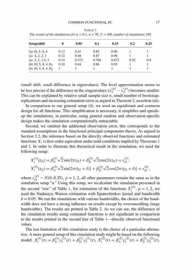
COMMON FUNCTIONAL PC 17
TABLE 1The results of the simulations for α = 0.1, n = 70, T = 100, number of simulations 250
Setup/shift 0 0.05 0.1 0.15 0.2 0.25
(a) 10, 5, 8, 4 0.13 0.41 0.85 0.96 1 1(a) 4, 2, 2, 1 0.12 0.48 0.87 0.96 1 1(a) 2, 1, 1.5, 2 0.14 0.372 0.704 0.872 0.92 0.9(b) 10, 5, 8, 4 D1 0.10 0.44 0.86 0.95 1 1(b) 10, 5, 8, 4 D2 1 1 1 1 1 1
(small shift, small difference in eigenvalues). The level approximation seems tobe less precise if the difference in the eingenvalues (λ(p)
1 − λ(p)2 ) becomes smaller.
This can be explained by relative small sample-size n, small number of bootstrap-replications and increasing estimation-error as argued in Theorem 2, assertion (iii).
In comparison to our general setup (4), we used an equidistant and commondesign for all functions. This simplification is necessary, it simplifies and speeds-up the simulations, in particular, using general random and observation-specificdesign makes the simulation computationally untractable.
Second, we omitted the additional observation error, this corresponds to thestandard assumptions in the functional principal components theory. As argued inSection 2.2, the inference based on the directly observed functions and estimatedfunctions Xi is first-order equivalent under mild conditions implied by Theorems 1and 2. In order to illustrate this theoretical result in the simulation, we used thefollowing setup:
X(1)i (tik) = β
(1)1i
√2 sin(2πtik) + β
(1)2i
√2 cos(2πtik) + ε
(1)ik ,
X(2)i (tik) = β
(2)1i
√2 sin{2π(tik + δ)} + β
(2)2i
√2 cos{2π(tik + δ)} + ε
(2)ik ,
where ε(p)ik ∼ N(0,0.25), p = 1,2, all other parameters remain the same as in the
simulation setup “a.” Using this setup, we recalculate the simulation presented inthe second “row” of Table 1, for estimation of the functions X
(p)i ,p = 1,2, we
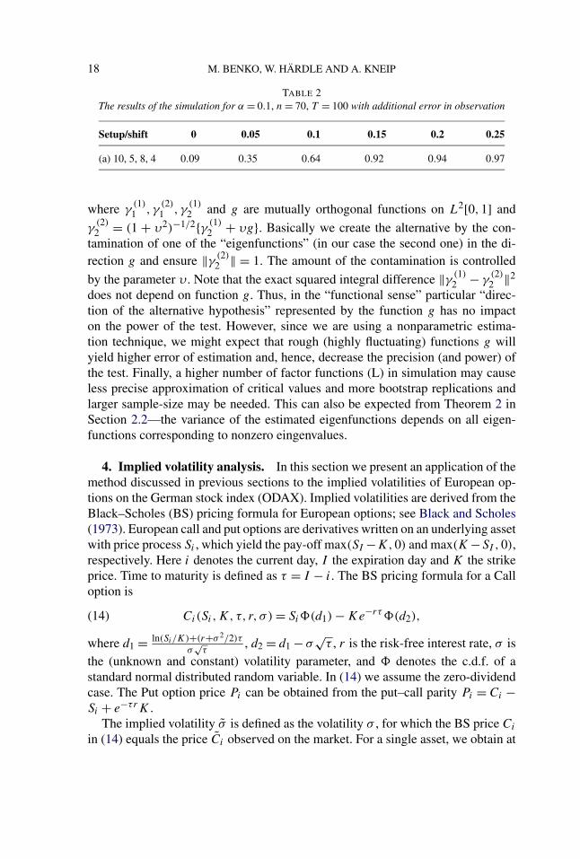
used the Nadaraya–Watson estimation with Epanechnikov kernel and bandwidthb = 0.05. We run the simulations with various bandwidths, the choice of the band-width does not have a strong influence on results except by oversmoothing (largebandwidths). The results are printed in Table 2. As we can see, the difference ofthe simulation results using estimated functions is not significant in comparisonto the results printed in the second line of Table 1—directly observed functionalvalues.
The last limitation of this simulation study is the choice of a particular alterna-tive. A more general setup of this simulation study might be based on the followingmodel: X
(1)i (t) = β
(1)1i γ
(1)1 (t) + β
(1)2i γ
(1)2 (t), X
(2)i (t) = β
(2)1i γ
(2)1 (t) + β
(2)2i γ
(2)2 (t),
18 M. BENKO, W. HÄRDLE AND A. KNEIP
TABLE 2The results of the simulation for α = 0.1, n = 70, T = 100 with additional error in observation
Setup/shift 0 0.05 0.1 0.15 0.2 0.25
(a) 10, 5, 8, 4 0.09 0.35 0.64 0.92 0.94 0.97
where γ(1)1 , γ
(2)1 , γ
(1)2 and g are mutually orthogonal functions on L2[0,1] and
γ(2)2 = (1 + υ2)−1/2{γ (1)
2 + υg}. Basically we create the alternative by the con-tamination of one of the “eigenfunctions” (in our case the second one) in the di-rection g and ensure ‖γ (2)
2 ‖ = 1. The amount of the contamination is controlled
by the parameter υ . Note that the exact squared integral difference ‖γ (1)2 − γ
(2)2 ‖2
does not depend on function g. Thus, in the “functional sense” particular “direc-tion of the alternative hypothesis” represented by the function g has no impacton the power of the test. However, since we are using a nonparametric estima-tion technique, we might expect that rough (highly fluctuating) functions g willyield higher error of estimation and, hence, decrease the precision (and power) ofthe test. Finally, a higher number of factor functions (L) in simulation may causeless precise approximation of critical values and more bootstrap replications andlarger sample-size may be needed. This can also be expected from Theorem 2 inSection 2.2—the variance of the estimated eigenfunctions depends on all eigen-functions corresponding to nonzero eingenvalues.
4. Implied volatility analysis. In this section we present an application of themethod discussed in previous sections to the implied volatilities of European op-tions on the German stock index (ODAX). Implied volatilities are derived from theBlack–Scholes (BS) pricing formula for European options; see Black and Scholes(1973). European call and put options are derivatives written on an underlying assetwith price process Si , which yield the pay-off max(SI −K,0) and max(K −SI ,0),respectively. Here i denotes the current day, I the expiration day and K the strikeprice. Time to maturity is defined as τ = I − i. The BS pricing formula for a Calloption is
Ci(Si,K, τ, r, σ ) = Si�(d1) − Ke−rτ�(d2),(14)
where d1 = ln(Si/K)+(r+σ 2/2)τ
σ√
τ, d2 = d1 − σ
√τ , r is the risk-free interest rate, σ is
the (unknown and constant) volatility parameter, and � denotes the c.d.f. of astandard normal distributed random variable. In (14) we assume the zero-dividendcase. The Put option price Pi can be obtained from the put–call parity Pi = Ci −Si + e−τrK .
The implied volatility σ is defined as the volatility σ , for which the BS price Ci
in (14) equals the price Ci observed on the market. For a single asset, we obtain at

COMMON FUNCTIONAL PC 19
each time point (day i) and for each maturity τ a IV function σ τi (K). Practitioners
often rescale the strike dimension by plotting this surface in terms of (futures)moneyness κ = K/Fi(τ ), where Fi(τ ) = Sie
rτ .Clearly, for given parameters Si, r,K, τ the mapping from prices to IVs is a one-
to-one mapping. The IV is often used for quoting the European options in financialpractice, since it reflects the “uncertainty” of the financial market better than theoption prices. It is also known that if the stock price drops, the IV raises (so-calledleverage effect), motivates hedging strategies based on IVs. Consequently, for thepurpose of this application, we will regard the BS–IV as an individual financialvariable. The practical relevance of such an approach is justified by the volatilitybased financial products such as VDAX, which are commonly traded on the optionmarkets.
The goal of this analysis is to study the dynamics of the IV functions for dif-ferent maturities. More specifically, our aim is to construct low dimensional factormodels based on the truncated Karhunen–Loève expansions (1) for the log-returnsof the IV functions of options with different maturities and compare these factormodels using the methodology presented in the previous sections. Analysis of IVsbased on a low-dimensional factor model gives directly a descriptive insight intothe structure of distribution of the log-IV-returns—structure of the factors and em-pirical distribution of the factor loadings may be a good starting point for furtherpricing models. In practice, such a factor model can also be used in Monte Carlobased pricing methods and for risk-management (hedging) purposes. For compre-hensive monographs on IV and IV-factor models, see Hafner (2004) or Fengler(2005b).
The idea of constructing and analyzing the factor models for log-IV-returnsfor different maturities was originally proposed by Fengler, Härdle and Villa(2003), who studied the dynamics of the IV via PCA on discretized IV func-tions for different maturity groups and tested the Common Principal Compo-nents (CPC) hypotheses (equality of eigenvectors and eigenspaces for differentgroups). Fengler, Härdle and Villa (2003) proposed a PCA-based factor modelfor log-IV-returns on (short) maturities 1, 2 and 3 months and grid of moneyness[0.85,0.9,0.95,1,1.05,1.1]. They showed that the factor functions do not sig-nificantly differ and only the factor loadings differ across maturity groups. Theirmethod relies on the CPC methodology introduced by Flury (1988) which is basedon maximum likelihood estimation under the assumption of multivariate normal-ity. The log-IV-returns are extracted by the two-dimensional Nadaraya–Watsonestimate.
The main aim of this application is to reconsider their results in a functionalsense. Doing so, we overcome two basic weaknesses of their approach. First, thefactor model proposed by Fengler, Härdle and Villa (2003) is performed only ona sparse design of moneyness. However, in practice (e.g., in Monte Carlo pric-ing methods), evaluation of the model on a fine grid is needed. Using the func-tional PCA approach, we may overcome this difficulty and evaluate the factor
20 M. BENKO, W. HÄRDLE AND A. KNEIP
model on an arbitrary fine grid. The second difficulty of the procedure proposedby Fengler, Härdle and Villa (2003) stems from the data design—on the exchangewe cannot observe options with desired maturity on each day and we need toestimate them from the IV-functions with maturities observed on the particularday. Consequently, the two-dimensional Nadaraya–Watson estimator proposed byFengler, Härdle and Villa (2003) results essentially in the (weighted) average ofthe IVs (with closest maturities) observed on a particular day, which may af-fect the test of the common eigenfunction hypothesis. We use the linear inter-
polation scheme in the total variance σ 2TOT,i(κ, τ )
def= (σ τi (κ))2τ, in order to re-
cover the IV functions with fixed maturity (on day i). This interpolation schemeis based on the arbitrage arguments originally proposed by Kahalé (2004) forzero-dividend and zero-interest rate case and generalized for deterministic inter-est rate by Fengler (2005a). More precisely, having IVs with maturities observedon a particular day i: σ
τji
i (κ), ji = 1, . . . , pτi, we calculate the corresponding to-
tal variance σTOT,i(κ, τji). From these total variances we linearly interpolate the
total variance with the desired maturity from the nearest maturities observed onday i. The total variance can be easily transformed to corresponding IV σ τ
i (κ). As
the last step, we calculate the log-returns � log σ τi (κ)
def= log σ τi+1(κ) − log σ τ
i (κ).The log-IV-returns are observed for each maturity τ on a discrete grid κτ
ik . We as-sume that observed log-IV-return � log σ τ
i (κτik) consists of true log-return of the
IV function denoted by � logσ τi (κτ
ik) and possibly of some additional error ετik .
By setting Y τik := � log σ τ
i (κτik), Xτ
i (κ) := � logστi (κ), we obtain an analogue of
the model (4) with the argument κ :
Y τik = Xτ
i (κik) + ετik, i = 1, . . . , nτ .(15)
In order to simplify the notation and make the connection with the theoretical partclear, we will use the notation of (15).
For our analysis we use a recent data set containing daily data from Janu-ary 2004 to June 2004 from the German–Swiss exchange (EUREX). Violationsof the arbitrage-free assumptions (“obvious” errors in data) were corrected us-ing the procedure proposed by Fengler (2005a). Similarly to Fengler, Härdle andVilla (2003), we excluded options with maturity smaller then 10 days, since theseoption-prices are known to be very noisy, partially because of a special and arbi-trary setup in the pricing systems of the dealers. Using the interpolation schemedescribed above, we calculate the log-IV-returns for two maturity groups: “1M”group with maturity τ = 0.12 (measured in years) and “3M” group with matu-rity τ = 0.36. The observed log-IV-returns are denoted by Y 1M
ik , k = 1, . . . ,K1Mi ,
Y 3Mik , k = 1, . . . ,K3M
i . Since we ensured that for no i, the interpolation procedureuses data with the same maturity for both groups, this procedure has no impact onthe independence of both samples.
COMMON FUNCTIONAL PC 21
The underlying models based on the truncated version of (3) are as follows:
X1Mi (κ) = X1M(κ) +
L1M∑r=1
β1Mri γr
1M(κ), i = 1, . . . , n1M,(16)
X3Mi (κ) = X3M(κ) +
L3M∑r=1
β3Mri γr
3M(κ), i = 1, . . . , n3M.(17)
Models (16) and (17) can serve, for example, in a Monte Carlo pricing tool inthe risk management for pricing exotic options where the whole path of impliedvolatilities is needed to determine the price. Estimating the factor functions in (16)and (17) by eigenfunctions displayed in Figure 1, we only need to fit the (esti-mated) factor loadings β1M
ji and β3Mji . The pillar of the model is the dimension
reduction. Keeping the factor function fixed for a certain time period, we need toanalyze (two) multivariate random processes of the factor loadings. For the pur-poses of this paper we will focus on the comparison of factors from models (16)and (17) and the technical details of the factor loading analysis will not be dis-cussed here, since in this respect we refer to Fengler, Härdle and Villa (2003), whoproposed to fit the factor loadings by centered normal distributions with diagonalvariance matrix containing the corresponding eigenvalues. For a deeper discus-sion of the fitting of factor loadings using a more sophisticated approach, basicallybased on (possibly multivariate) GARCH models; see Fengler (2005b).
From our data set we obtained 88 functional observations for the 1M group(n1M ) and 125 observations for the 3M group (n3M ). We will estimate the modelon the interval for futures moneyness κ ∈ [0.8,1.1]. In comparison to Fengler,Härdle and Villa (2003), we may estimate models (16) and (17) on an arbitraryfine grid (we used an equidistant grid of 500 points on the interval [0.8,1.1]). Forillustration, the Nadaraya–Watson (NW) estimator of resulting log-returns is plot-ted in Figure 2. The smoothing parameters have been chosen in accordance withthe requirements in Section 2.2. As argued in Section 2.2, we should use smallsmoothing parameters in order to avoid a possible bias in the estimated eigenfunc-tions. Thus, we use for each i essentially the smallest bandwidth bi that guaranteesthat estimator Xi is defined on the entire support [0.8,1.1].
Using the procedures described in Section 2.1, we first estimate the eigenfunc-tions of both maturity groups. The estimated eigenfunctions are plotted in Figure 1.The structure of the eigenfunctions is in accordance with other empirical studieson IV-surfaces. For a deeper discussion and economical interpretation, see, for ex-ample, Fengler, Härdle and Mammen (2007) or Fengler, Härdle and Villa (2003).
Clearly, the ratio of the variance explained by the kth factor function is givenby the quantity ν1M
k = λ1Mk /
∑n1M
j=1 λ1Mj for the 1M group and, correspondingly, by
ν3Mk for the 3M group. In Table 3 we list the contributions of the factor functions.
Looking at Table 3, we can see that 4th factor functions explain less than 1% ofthe variation. This number was the “threshold” for the choice of L1M and L2M .

22 M. BENKO, W. HÄRDLE AND A. KNEIP
FIG. 2. Nadaraya–Watson estimate of the log-IV-returns for maturity 1M (left figure) and 3M (rightfigure). The bold line is the sample mean of the corresponding group.
We can observe (see Figure 1) that the factor functions for both groups aresimilar. Thus, in the next step we use the bootstrap test for testing the equalityof the factor functions. We use 2000 bootstrap replications. The test of equal-ity of the eigenfunctions was rejected for the first eigenfunction for the analyzedtime period (January 2004–June 2004) at a significance level α = 0.05 (P-value0.01). We may conclude that the (first) factor functions are not identical in thefactor model for both maturity groups. However, from a practical point of view,we are more interested in checking the appropriateness of the entire models fora fixed number of factors: L = 2 or L = 3 in (16) and (17). This requirementtranslates into the testing of the equality of eigenspaces. Thus, in the next stepwe use the same setup (2000 bootstrap replications) to test the hypotheses thatthe first two and first three eigenfunctions span the same eigenspaces E1M
L andE3M
L . None of the hypotheses for L = 2 and L = 3 is rejected at significancelevel α = 0.05 (P-value is 0.61 for L = 2 and 0.09 for L = 3). Summarizing,even in the functional sense we have no significant reason to reject the hypothe-sis of common eigenspaces for these two maturity groups. Using this hypothesis,
TABLE 3Variance explained by the eigenfunctions
Var. explained 1M Var. explained 3M
ντ1 89.9% 93.0%
ντ2 7.7% 4.2%
ντ3 1.7% 1.0%
ντ4 0.6% 0.4%

COMMON FUNCTIONAL PC 23
the factors governing the movement of the returns of IV surface are invariant totime to maturity, only their relative importance can vary. This leads to the com-mon factor model: Xτ
i (κ) = Xτ (κ)+∑Lτ
r=1 βτri γr (κ), i = 1, . . . , nτ , τ = 1M,3M,
where γr := γ 1Mr = γ 3M
r . Beside contributing to the understanding of the struc-ture of the IV function dynamics, the common factor model helps us to reducethe number of functional factors by half compared to models (16) and (17). Fur-thermore, from the technical point of view, we also obtain an additional dimen-sion reduction and higher estimation precision, since under this hypothesis wemay estimate the eigenfunctions from the (individually centered) pooled sampleXi(κ)1M, i = 1, . . . , n1M , X3M
i (κ), i = 1, . . . , n3M . The main improvement com-pared to the multivariate study by Fengler, Härdle and Villa (2003) is that our test isperformed in the functional sense – it does not depend on particular discretizationand our factor model can be evaluated on an arbitrary fine grid.
APPENDIX: MATHEMATICAL PROOFS
In the following, ‖v‖ = (∫ 1
0 v(t)2 dt)1/2 will denote the L2-norm for any squareintegrable function v. At the same time, ‖a‖ = (1
k
∑ki=1 a2
i )1/2 will indicate the
Euclidean norm, whenever a ∈ Rk is a k-vector for some k ∈ N.
In the proof of Theorem 1, Eε and Varε denote expectation and variance withrespect to ε only (i.e., conditional on tij and Xi).
PROOF OF THEOREM 1. Recall the definition of the χi(t) and note thatχi(t) = χX
i (t) + χεi (t), where
χεi (t) =
Ti∑j=1
εi(j)I
(t ∈[ti(j−1) + ti(j)
2,ti(j) + ti(j+1)
2
)),
as well as
χXi (t) =
Ti∑j=1
Xi
(ti(j)
)I
(t ∈[ti(j−1) + ti(j)
2,ti(j) + ti(j+1)
2
))
for t ∈ [0,1], ti(0) = −ti(1) and ti(Ti+1) = 2 − ti(Ti). Similarly, χ∗i (t) = χ
X∗i (t) +
χε∗i (t).
By Assumption 2, E(|ti(j) − ti(j−1)|s) = O(T −s) for s = 1, . . . ,4, and the con-vergence is uniform in j < n. Our assumptions on the structure of Xi together withsome straightforward Taylor expansions then lead to
〈χi,χj 〉 = 〈Xi,Xj 〉 + Op(1/T )
and
〈χi,χ∗i 〉 = ‖Xi‖2 + Op(1/T ).
24 M. BENKO, W. HÄRDLE AND A. KNEIP
Moreover,
Eε(〈χεi , χX
j 〉) = 0, Eε(‖χεi ‖2) = σ 2
i ,
Eε(〈χεi , χε∗
i 〉) = 0, Eε(〈χεi , χε∗
i 〉2) = Op(1/T ),
Eε(〈χεi , χX
j 〉2) = Op(1/T ), Eε(〈χεi , χX
j 〉〈χεk ,χX
l 〉) = 0 for i = k,
Eε(〈χεi , χε
j 〉〈χεi , χε
k 〉) = 0 for j = k and Eε(‖χεi ‖4) = Op(1)
hold (uniformly) for all i, j = 1, . . . , n.Consequently, Eε(‖χ‖2 − ‖X‖2) = Op(T −1 + n−1).When using these relations, it is easily seen that for all i, j = 1, . . . , n
Mij − Mij = Op(T −1/2 + n−1) and(18)
tr{(M − M)2}1/2 = Op(1 + nT −1/2).
Since the orthonormal eigenvectors pq of M satisfy ‖pq‖ = 1, we furthermoreobtain for any i = 1, . . . , n and all q = 1,2, . . .
n∑j=1
pjq
{Mij − Mij −
∫ 1
0χε
i (t)χXj (t) dt
}= Op(T −1/2 + n−1/2),(19)
as well asn∑
j=1
pjq
∫ 1
0χε
i (t)χXj (t) dt = Op
(n1/2
T 1/2
)(20)
andn∑
i=1
ai
n∑j=1
pjq
∫ 1
0χε
i (t)χXj (t) dt = Op
(n1/2
T 1/2
)(21)
for any further vector a with ‖a‖ = 1.Recall that the j th largest eigenvalue lj satisfies nλj = lj . Since by assumption
infs =r |λr − λs | > 0, the results of Dauxois, Pousse and Romain (1982) implythat λr converges to λr as n → ∞, and sups =r
1|λr−λs | = Op(1), which leads to
sups =r1
|lr−ls | = Op(1/n). Assertion (a) of Lemma A of Kneip and Utikal (2001)together with (18)–(21) then implies that∣∣∣∣λr − lr
n
∣∣∣∣= n−1|lr − lr | = n−1|p�r (M − M)pr | + Op(T −1 + n−1)
(22)= Op{(nT )−1/2 + T −1 + n−1}.
When analyzing the difference between the estimated and true eigenvectors pr
and pr , assertion (b) of Lemma A of Kneip and Utikal (2001) together with (18)lead to
pr − pr = −Sr (M − M)pr + Rr , with ‖Rr‖ = Op(T −1 + n−1)(23)

COMMON FUNCTIONAL PC 25
and Sr =∑s =r
1ls−lr
psp�s . Since sup‖a‖=1 a�Sra ≤ sups =r
1|lr−ls | = Op(1/n), we
can conclude that
‖pr − pr‖ = Op(T −1/2 + n−1),(24)
and our assertion on the sequence n−1∑i (βri − βri;T )2 is an immediate conse-
quence.Let us now consider assertion (ii). The well-known properties of local linear
estimators imply that |Eε{Xi(t) − Xi(t)}| = Op(b2), as well as Varε{Xi(t)} =Op{T b}, and the convergence is uniform for all i, n. Furthermore, due to the inde-pendence of the error term εij , Covε{Xi(t), Xj (t)} = 0 for i = j . Therefore,∣∣∣∣∣γr (t) − 1√
lr
n∑i=1
pirXi(t)
∣∣∣∣∣= Op
(b2 + 1√
nT b
).
On the other hand, (18)–(24) imply that with X(t) = (X1(t), . . . , Xn(t))�∣∣∣∣∣γr;T (t) − 1√
lr
n∑i=1
pirXi(t)
∣∣∣∣∣=∣∣∣∣∣ 1√
lr
n∑i=1
(pir − pir)Xi(t) + 1√lr
n∑i=1
(pir − pir){Xi(t) − Xi(t)}∣∣∣∣∣
+ Op(T −1 + n−1)
= ‖SrX(t)‖√lr
∣∣∣∣p�r (M − M)Sr
X(t)
‖SrX(t)‖∣∣∣∣
+ Op(b2T −1/2 + T −1b−1/2 + n−1)
= Op(n−1/2T −1/2 + b2T −1/2 + T −1b−1/2 + n−1).
This proves the theorem. �
PROOF OF THEOREM 2. First consider assertion (i). By definition,
X(t) − μ(t) = n−1n∑
i=1
{Xi(t) − μ(t)} =∑r
(n−1
n∑i=1
βri
)γr(t).
Recall that, by assumption, βri are independent, zero mean random variables withvariance λr , and that the above series converges with probability 1. When definingthe truncated series
V (q) =q∑
r=1
(n−1
n∑i=1
βri
)γr(t),
standard central limit theorems therefore imply that√
nV (q) is asymptoticallyN(0,
∑qr=1 λrγr(t)
2) distributed for any possible q ∈ N.

26 M. BENKO, W. HÄRDLE AND A. KNEIP
The assertion of a N(0,∑∞
r=1 λrγr(t)2) limiting distribution now is a conse-
quence of the fact that for all δ1, δ2 > 0 there exists a qδ such that P {|√nV (q) −√n∑
r (n−1∑n
i=1 βri)γr(t)| > δ1} < δ2 for all q ≥ qδ and all n sufficiently large.In order to prove assertions (i) and (ii), consider some fixed r ∈ {1,2, . . .} with
λr−1 > λr > λr+1. Note that � as well as �n are nuclear, self-adjoint and non-negative linear operators with �v = ∫
σ(t, s)v(s) ds and �nv = ∫σ (t, s)v(s) ds,
v ∈ L2[0,1]. For m ∈ N, let �m denote the orthogonal projector from L2[0,1]into the m-dimensional linear space spanned by {γ1, . . . , γm}, that is, �mv =∑m
j=1〈v, γj 〉γj , v ∈ L2[0,1]. Now consider the operator �m�n�m, as well as
its eigenvalues and corresponding eigenfunctions denoted by λ1,m ≥ λ2,m ≥ · · ·and γ1,m, γ2,m, . . . , respectively. It follows from well-known results in the Hilbertspace theory that �m�n�m converges strongly to �n as m → ∞. Furthermore, weobtain (Rayleigh–Ritz theorem)
limm→∞ λr,m = λr and lim
m→∞‖γr − γr,m‖ = 0 if λr−1 > λr > λr+1.(25)
Note that under the above condition γr is uniquely determined up to sign, and recallthat we always assume that the right “versions” (with respect to sign) are used sothat 〈γr , γr,m〉 ≥ 0. By definition, βji = ∫
γj (t){Xi(t) − μ(t)}dt , and therefore,∫γj (t){Xi(t) − X(t)}dt = βji − βj , as well as Xi − X =∑
j (βji − βj )γj , where
βj = 1n
∑ni=1 βji . When analyzing the structure of �m�n�m more deeply, we can
verify that �m�n�mv = ∫σm(t, s)v(s) ds, v ∈ L2[0,1], with
σm(t, s) = gm(t)��mgm(s),
where gm(t) = (γ1(t), . . . , γm(t))�, and where �m is the m × m matrix with el-ements { 1
n
∑ni=1(βji − βj )(βki − βk)}j,k=1,...,m. Let λ1(�m) ≥ λ2(�m) ≥ · · · ≥
λm(�m) and ζ1,m, . . . , ζm,m denote eigenvalues and corresponding eigenvectors of�m. Some straightforward algebra then shows that
λr,m = λr(�m), γr,m = gm(t)�ζr,m.(26)
We will use �m to represent the m × m diagonal matrix with diagonal en-tries λ1 ≥ · · · ≥ λm. Obviously, the corresponding eigenvectors are given by them-dimensional unit vectors denoted by e1,m, . . . , em,m. Lemma A of Kneip andUtikal (2001) now implies that the differences between eigenvalues and eigenvec-tors of �m and �m can be bounded by
λr,m − λr = tr{er,me�r,m(�m − �m)} + Rr,m,
(27)
with Rr,m ≤ 6 sup‖a‖=1 a�(�m − �m)2a
mins |λs − λr | ,
ζr,m − er,m = −Sr,m(�m − �m)er,m + R∗r,m,
(28)
with ‖R∗r,m‖ ≤ 6 sup‖a‖=1 a�(�m − �m)2a
mins |λs − λr |2 ,
COMMON FUNCTIONAL PC 27
where Sr,m =∑s =r
1λs−λr
es,me�s,m.
Assumption 1 implies E(βr ) = 0, Var(βr ) = λrn
, and with δii = 1, as well asδij = 0 for i = j , we obtain
E{
sup‖a‖=1
a�(�m − �m)2a
}≤ E{tr[(�m − �m)2]}
= E
{m∑
j,k=1
[1
n
n∑i=1
(βji − βj )(βki − βk) − δjkλj
]2}(29)
≤ E
{ ∞∑j,k=1
[1
n
n∑i=1
(βji − βj )(βki − βk) − δjkλj
]2}
= 1
n
(∑j
∑k
E{β2jiβ
2ki})
+ O(n−1) = O(n−1),
for all m. Since tr{er,me�r,m(�m −�m)} = 1
n
∑ni=1(βri − βr )
2 −λr , (25), (26), (27)and (29) together with standard central limit theorems imply that
√n(λr − λr) = 1√
n
n∑i=1
(βri − βr )2 − λr + Op(n−1/2)
= 1√n
n∑i=1
[(βri)2 − E{(βri)
2}] + Op(n−1/2)(30)
L→ N(0,�r).
It remains to prove assertion (iii). Relations (26) and (28) lead to
γr,m(t) − γr(t) = gm(t)�(ζr,m − er,m)
= −m∑
s =r
{1
n(λs − λr)
n∑i=1
(βsi − βs)(βri − βr )
}γs(t)(31)
+ gm(t)�R∗r,m,
where due to (29) the function gm(t)�R∗r,m satisfies
E(‖g�mR∗
r,m‖) = E(‖R∗r,m‖)
≤ 6
nmins |λs − λr |2(∑
j
∑k
E{β2jiβ
2ki})
+ O(n−1),
28 M. BENKO, W. HÄRDLE AND A. KNEIP
for all m. By Assumption 1, the series in (31) converge with probability 1 as m →∞.
Obviously, the event λr−1 > λr > λr+1 occurs with probability 1. Since m isarbitrary, we can therefore conclude from (25) and (31) that
γr (t) − γr(t)
= −∑s =r
{1
n(λs − λr)
n∑i=1
(βsi − βs)(βri − βr )
}γs(t) + R∗
r (t)(32)
= −∑s =r
{1
n(λs − λr)
n∑i=1
βsiβri
}γs(t) + Rr(t),
where ‖R∗r ‖ = Op(n−1), as well as ‖Rr‖ = Op(n−1). Moreover,
√n ×∑
s =r{ 1n(λs−λr )
∑ni=1 βsiβri}γs(t) is a zero mean random variable with variance∑
q =r
∑s =r
E[β2riβqiβsi ]
(λq−λr )(λs−λr )γq(t)γs(t) < ∞. By Assumption 1, it follows from stan-
dard central limit arguments that for any q ∈ N the truncated series√
nW(q)def=√
n∑q
s=1,s =r [ 1n(λs−λr )
∑ni=1 βsiβri]γs(t) is asymptotically normal distributed. The
asserted asymptotic normality of the complete series then follows from an argu-ment similar to the one used in the proof of assertion (i). �
PROOF OF THEOREM 3. The results of Theorem 2 imply that
n�1 =∫ (∑
r
1√q1n1
n1∑i=1
β(1)ri γ (1)
r (t)
(33)
−∑r
1√q2n2
n2∑i=1
β(2)ri γ (2)
r (t)
)2
dt.
Furthermore, independence of X(1)i and X
(2)i together with (30) imply that
√n[λ(1)
r − λ(1)r − {λ(2)
r − λ(2)r
}] L→ N
(0,
�(1)r
q1+ �
(2)r
q2
)and
(34)n
�(1)r /q1 + �
(2)r /q2
�3,rL→ χ2
1 .
Furthermore, (32) leads to
n�2,r =∥∥∥∥∥∑
s =r
{1
√q1n1(λ
(1)s − λ
(1)r )
n1∑i=1
β(1)si β
(1)ri
}γ (1)s
(35)
−∑s =r
{1
√q2n2(λ
(2)s − λ
(2)r )
n2∑i=1
β(2)si β
(2)ri
}γ (2)s
∥∥∥∥∥2
+ Op(n−1/2)
COMMON FUNCTIONAL PC 29
and
n�4,L = n
∫ ∫ [ L∑r=1
γ (1)r (t)
{γ (1)r (u) − γ (1)
r (u)}
+ γ (1)r (u)
{γ (1)r (t) − γ (1)
r (t)}
−L∑
r=1
γ (2)r (t)
{γ (2)r (u) − γ (2)
r (u)}
+ γ (2)r (u)
{γ (2)r (t) − γ (2)
r (t)}]2
dt du + Op(n−1/2)
=∫ ∫ [ L∑
r=1
∑s>L
{1
√q1n1(λ
(1)s − λ
(1)r )
n1∑i=1
β(1)si β
(1)ri
}(36)
× {γ (1)r (t)γ (1)
s (u) + γ (1)r (u)γ (1)
s (t)}
−L∑
r=1
∑s>L
{1
√q2n2(λ
(2)s − λ
(2)r )
n2∑i=1
β(2)si β
(2)ri
}
× {γ (2)r (t)γ (2)
s (u) + γ (2)r (u)γ (2)
s (t)}]2
dt du
+ Op(n−1/2).
In order to verify (36), note that∑L
r=1∑L
s=1,s =r1
(λ(p)s −λ
(p)r )
aras = 0 for p = 1,2
and all possible sequences a1, . . . , aL. It is clear from our assumptions that allsums involved converge with probability 1. Recall that E(β
(p)ri β
(p)si ) = 0, p = 1,2
for r = s.
It follows that X(p)r := 1√
qpnp
∑s =r
∑np
i=1β
(p)si β
(p)ri
λ(p)s −λ
(p)r
γ(p)s , p = 1,2, is a continu-
ous, zero mean random function on L2[0,1], and, by assumption, E(‖X(p)r ‖2) <
∞. By Hilbert space central limit theorems [see, e.g., Araujo and Giné (1980)],X
(p)r thus converges in distribution to a Gaussian random function ξ
(p)r as
n → ∞. Obviously, ξ(1)r is independent of ξ
(2)r . We can conclude that n�4,L
possesses a continuous limit distribution F4,L defined by the distribution of∫∫ [∑Lr=1{ξ (1)
r (t)γ(1)r (u) + ξ
(1)r (u)γ
(1)r (t)} − ∑L
r=1{ξ (2)r (t)γ
(2)r (u) + ξ
(2)r (u) ×
γ(2)r (t)}]2 dt du. Similar arguments show the existence of continuous limit dis-
tributions F1 and F2,r of n�1 and n�2,r .For given q ∈ N, define vectors b
(p)i1 = (β
(p)1i , . . . , β
(p)qi , )� ∈ R
q , b(p)i2 =
(β(p)1i β
(p)ri , . . . , β
(p)r−1,iβ
(p)ri , β
(p)r+1,iβ
(p)ri , . . . , β
(p)qi β
(p)ri )� ∈ R
q−1 and bi3 = (β(p)1i β
(p)2i ,
30 M. BENKO, W. HÄRDLE AND A. KNEIP
. . . , β(p)qi β
(p)Li )� ∈ R
(q−1)L. When the infinite sums over r in (33), respectivelys = r in (35) and (36), are restricted to q ∈ N components (i.e.,
∑r and
∑s>L
are replaced by∑
r≤q and∑
L<s≤q ), then the above relations can generally bepresented as limits n� = limq→∞ n�(q) of quadratic forms
n�1(q) =
⎛⎜⎜⎜⎜⎝1√n1
n1∑i=1
b(1)i1
1√n2
n2∑i=1
b(2)i1
⎞⎟⎟⎟⎟⎠�
Qq1
⎛⎜⎜⎜⎜⎝1√n1
n1∑i=1
b(1)i1
1√n2
n2∑i=1
b(2)i1
⎞⎟⎟⎟⎟⎠ ,
n�2,r (q) =
⎛⎜⎜⎜⎜⎝1√n1
n1∑i=1
b(1)i2
1√n2
n2∑i=1
b(2)i2
⎞⎟⎟⎟⎟⎠�
Qq2
⎛⎜⎜⎜⎜⎝1√n1
n1∑i=1
b(1)i2
1√n2
n2∑i=1
b(2)i2
⎞⎟⎟⎟⎟⎠ ,(37)
n�4,L(q) =
⎛⎜⎜⎜⎜⎝1√n1
n1∑i=1
b(1)i3
1√n2
n2∑i=1
b(2)i3
⎞⎟⎟⎟⎟⎠�
Qq3
⎛⎜⎜⎜⎜⎝1√n1
n1∑i=1
b(1)i3
1√n2
n2∑i=1
b(2)i3
⎞⎟⎟⎟⎟⎠ ,
where the elements of the 2q ×2q , 2(q −1)×2(q −1) and 2L(q −1)×2L(q −1)
matrices Qq1 , Qq
2 and Qq3 can be computed from the respective (q-element) version
of (33)–(36). Assumption 1 implies that all series converge with probability 1 asq → ∞, and by (33)–(36), it is easily seen that for all ε, δ > 0 there exist someq(ε, δ), n(ε, δ) ∈ N such that
P(|n�1 − n�1(q)| > ε
)< δ, P
(|n�2,r − n�2,r (q)| > ε)< δ,
(38)P(|n�4,L − n�4,L(q)| > ε
)< δ
hold for all q ≥ q(ε, δ) and all n ≥ n(ε, δ). For any given q , we have E(bi1) =E(bi2) = E(bi3) = 0, and it follows from Assumption 1 that the respective covari-ance structures can be represented by finite covariance matrices �1,q , �2,q and�3,q . It therefore follows from our assumptions together with standard multivari-
ate central limit theorems that the vectors { 1√n1
∑n1i=1(b
(1)ik )�, 1√
n2
∑n2i=1(b
(2)ik )�}�,
k = 1,2,3, are asymptotically normal with zero means and covariance matrices�1,q , �2,q and �3,q . One can thus conclude that, as n → ∞,
n�1(q)L→ F1,q , n�2,r (q)
L→ F2,r,q , n�4,L(q)L→ F4,L,q,(39)
where F1,q ,F2,r,q ,F4,L,q denote the continuous distributions of the quadraticforms z�
1 Qq1z1, z�
2 Qq2z2, z�
3 Qq3z3 with z1 ∼ N(0,�1,q), z2 ∼ N(0,�2,q), z3 ∼
COMMON FUNCTIONAL PC 31
N(0,�3,q). Since ε, δ are arbitrary, (38) implies
limq→∞F1,q = F1, lim
q→∞F2,r,q = F2,r , limq→∞F4,L,q = F4,L.(40)
We now have to consider the asymptotic properties of bootstrapped eigenval-ues and eigenfunctions. Let X(p)∗ = 1
np
∑np
i=1 X(p)∗i , β
(p)∗ri = ∫
γ(p)r (t){X(p)∗
i (t) −μ(t)}, β
(p)∗r = 1
np
∑np
i=1 β(p)∗ri , and note that
∫γ
(p)r (t){X(p)∗
i (t) − X(p)∗(t)} =β
(p)∗ri − β
(p)∗r . When considering unconditional expectations, our assumptions im-
ply that for p = 1,2
E[β
(p)∗ri
]= 0, E[(
β(p)∗ri
)2]= λ(p)r ,
E[(
β(p)∗r
)2]= λ(p)r
np
, E{[(
β(p)∗ri
)2 − λ(p)r
]2}= �(p)r ,
E
{ ∞∑l,k=1
[1
np
np∑i=1
(β
(p)∗li − β
(p)∗l
)(β
(p)∗ki − β
(p)∗k
)− δlkλ(p)l
]2}(41)
= 1
np
(∑l
�(p)l +∑
l =k
λ(p)l λ
(p)k
)+ O(n−1
p ).
One can infer from (41) that the arguments used to prove Theorem 1 can begeneralized to approximate the difference between the bootstrap eigenvalues andeigenfunctions λ
(p)∗r , γ
(p)∗r and the true eigenvalues λ
(p)r , γ
(p)r . All infinite sums
involved converge with probability 1. Relation (30) then generalizes to√
np
(λ(p)∗
r − λ(p)r
)= √
np
(λ(p)∗
r − λ(p)r
)− √np
(λ(p)
r − λ(p)r
)= 1√
np
np∑i=1
(β
(p)∗ri − β(p)∗
r
)2(42)
− 1√np
np∑i=1
(β
(p)ri − β(p)
r
)2 + Op(n−1/2p )
= 1√np
np∑i=1
{(β
(p)∗ri
)2 − 1
np
np∑k=1
(β
(p)rk
)2}+ Op(n−1/2p ).
Similarly, (32) becomes
γ (p)∗r − γ (p)
r
= γ (p)∗r − γ (p)
r − (γ (p)r − γ (p)
r
)(43)
32 M. BENKO, W. HÄRDLE AND A. KNEIP
= −∑s =r
{1
λ(p)s − λ
(p)r
1
np
np∑i=1
(β
(p)∗si − β(p)∗
s
)(β
(p)∗ri − β(p)∗
r
)
− 1
λ(p)s − λ
(p)r
1
np
np∑i=1
(β
(p)si − β(p)
s
)(β
(p)ri − β(p)
r
)}γ (p)s (t)
+ R(p)∗r (t)
= −∑s =r
{1
λ(p)s − λ
(p)r
1
np
np∑i=1
(β
(p)∗si β
(p)∗ri − 1
np
np∑k=1
β(p)sk β
(p)rk
)}γ (p)s (t)
+ R(p)∗r (t),
where due to (28), (29) and (41), the remainder term satisfies ‖R(p)∗r ‖ = Op(n−1
p ).We are now ready to analyze the bootstrap versions �∗ of the different �.
First consider �∗3,r and note that {(β(p)∗
ri )2} are i.i.d. bootstrap resamples from
{(β(p)ri )2}. It therefore follows from basic bootstrap results that the conditional
distribution of 1√np
∑np
i=1[(β(p)∗ri )2 − 1
np
∑np
k=1(β(p)rk )2] given Xp converges to the
same N(0,�(p)r ) limit distribution as 1√
np
∑np
i=1[(β(p)ri )2 − E{(β(p)
ri )2}]. Together
with the independence of (β(1)∗ri )2 and (β
(2)∗ri )2, the assertion of the theorem is an
immediate consequence.Let us turn to �∗
1, �∗2,r and �∗
4,L. Using (41)–(43), it is then easily seen thatn�∗
1, n�∗2,r and n�∗
4,L admit expansions similar to (33), (35) and (36), when
replacing there 1√np
∑np
i=1 β(p)ri by 1√
np
∑np
i=1(β(p)∗ri − 1
np
∑np
k=1 β(p)rk ), as well as
1√np
∑np
i=1 β(p)si β
(p)ri by 1√
np
∑np
i=1(β(p)∗si β
(p)∗ri − 1
np
∑np
k=1 β(p)sk β
(p)rk ).
Replacing β(p)ri , β
(p)si by β
(p)∗ri , β(p)∗
si leads to bootstrap analogs b(p)∗ik of the vec-
tors b(p)ik , k = 1,2,3. For any q ∈ N, define bootstrap versions n�∗
1(q), n�∗2,r (q)
and n�∗4,L(q) of n�1(q), n�2,r (q) and n�4,L(q) by using ( 1√
n1
∑n1i=1(b
(1)∗ik −
1n1
∑n1k=1 b
(1)ik )�, 1√
n2
∑n2i=1(b
(2)∗ik − 1
n2
∑n2k=1 b
(2)ik )�) instead of ( 1√
n1
∑n1i=1(b
(1)ik )�,
1√n2
∑n2i=1(b
(2)ik )�), k = 1,2,3, in (37). Applying again (41)–(43), one can con-
clude that for any ε > 0 there exists some q(ε) such that, as n → ∞,
P(|n�∗
1 − n�∗1(q)| < ε
)→ 1,
P(|n�∗
2,r − n�∗2,r (q)| < ε
)→ 1,(44)
P(|n�∗
4,L − n�∗4,L(q)| < ε
)→ 1
hold for all q ≥ q(ε). Of course, (44) generalizes to the conditional probabilitiesgiven X1, X2.

COMMON FUNCTIONAL PC 33
In order to prove the theorem, it thus only remains to show that for any given q
and all δ ∣∣P(n�(q) ≥ δ)− P
(n�∗(q) ≥ δ| X1,X2
)∣∣= Op(1)(45)
hold for either �(q) = �1(q) and �∗(q) = �∗1(q), �(q) = �2,r (q) and �∗(q) =
�∗2,r (q), or �(q) = �4,L(q) and �∗(q) = �∗
4,L(q). But note that for k =1,2,3,E(bik) = 0, {b(j)∗
ik } are i.i.d. bootstrap resamples from {b(p)ik }, and E(b
(p)∗ik |
X1,X2) = 1np
∑np
k=1 b(p)ik are the corresponding conditional means. It therefore fol-
lows from basic bootstrap results that as n → ∞ the conditional distribution of( 1√
n1
∑n1i=1(b
(1)∗ik − 1
n1
∑n1k=1 b
(1)ik )�, 1√
n2
∑n2i=1(b
(2)∗ik − 1
n2
∑n2k=1 b
(2)ik )�) given X1,
X2 converges to the same N(0,�k,q) limit distribution as ( 1√n1
∑n1i=1(b
(1)ik )�,
1√n2
∑n2i=1, (b
(2)ik )�). This obviously holds for all q ∈ N, and (45) is an immedi-
ate consequence. The theorem then follows from (38), (39), (40), (44) and (45).�
REFERENCES
ARAUJO, A. and GINÉ, E. (1980). The Central Limit Theorem for Real and Banach Valued RandomVariables. Wiley, New York. MR0576407
BESSE, P. and RAMSAY, J. (1986). Principal components of sampled functions. Psychometrika 51285–311. MR0848110
BLACK, F. and SCHOLES, M. (1973). The pricing of options and corporate liabilities. J. PoliticalEconomy 81 637–654.
DAUXOIS, J., POUSSE, A. and ROMAIN, Y. (1982). Asymptotic theory for the principal componentanalysis of a vector random function: Some applications to statistical inference. J. MultivariateAnal. 12 136–154. MR0650934
FENGLER, M. (2005a). Arbitrage-free smoothing of the implied volatility surface. SFB 649 Discus-sion Paper No. 2005–019, SFB 649, Humboldt-Universität zu Berlin.
FENGLER, M. (2005b). Semiparametric Modeling of Implied Volatility. Springer, Berlin.MR2183565
FENGLER, M., HÄRDLE, W. and VILLA, P. (2003). The dynamics of implied volatilities: A commonprinciple components approach. Rev. Derivative Research 6 179–202.
FENGLER, M., HÄRDLE, W. and MAMMEN, E. (2007). A dynamic semiparametric factor modelfor implied volatility string dynamics. Financial Econometrics 5 189–218.
FERRATY, F. and VIEU, P. (2006). Nonparametric Functional Data Analysis. Springer, New York.MR2229687
FLURY, B. (1988). Common Principal Components and Related Models. Wiley, New York.MR0986245
GIHMAN, I. I. and SKOROHOD, A. V. (1973). The Theory of Stochastic Processes. II. Springer, NewYork. MR0375463
HALL, P. and HOSSEINI-NASAB, M. (2006). On properties of functional principal componentsanalysis. J. Roy. Statist. Soc. Ser. B 68 109–126. MR2212577
HALL, P., MÜLLER, H. G. and WANG, J. L. (2006). Properties of principal components methodsfor functional and longitudinal data analysis. Ann. Statist. 34 1493–1517. MR2278365
HALL, P., KAY, J. W. and TITTERINGTON, D. M. (1990). Asymptotically optimal difference-basedestimation of variance in nonparametric regression. Biometrika 77 520–528. MR1087842
34 M. BENKO, W. HÄRDLE AND A. KNEIP
HAFNER, R. (2004). Stochastic Implied Volatility. Springer, Berlin. MR2090447HÄRDLE, W. and SIMAR, L. (2003). Applied Multivariate Statistical Analysis. Springer, Berlin.
MR2061627KAHALÉ, N. (2004). An arbitrage-free interpolation of volatilities. Risk 17 102–106.KNEIP, A. and UTIKAL, K. (2001). Inference for density families using functional principal compo-
nents analysis. J. Amer. Statist. Assoc. 96 519–531. MR1946423LACANTORE, N., MARRON, J. S., SIMPSON, D. G., TRIPOLI, N., ZHANG, J. T. and COHEN, K.
L. (1999). Robust principal component analysis for functional data. Test 8 1–73. MR1707596PEZZULLI, S. D. and SILVERMAN, B. (1993). Some properties of smoothed principal components
analysis for functional data. Comput. Statist. 8 1–16. MR1220336RAMSAY, J. O. and DALZELL, C. J. (1991). Some tools for functional data analysis (with discus-
sion). J. Roy. Statist. Soc. Ser. B 53 539–572. MR1125714RAMSAY, J. and SILVERMAN, B. (2002). Applied Functional Data Analysis. Springer, New York.
MR1910407RAMSAY, J. and SILVERMAN, B. (2005). Functional Data Analysis. Springer, New York.
MR2168993RAO, C. (1958). Some statistical methods for comparison of growth curves. Biometrics 14 1–17.RICE, J. and SILVERMAN, B. (1991). Estimating the mean and covariance structure nonparametri-
cally when the data are curves. J. Roy. Statist. Soc. Ser. B 53 233–243. MR1094283SILVERMAN, B. (1996). Smoothed functional principal components analysis by choice of norm.
Ann. Statist. 24 1–24. MR1389877TYLER, D. E. (1981). Asymptotic inference for eigenvectors. Ann. Statist. 9 725–736. MR0619278YAO, F., MÜLLER, H. G. and WANG, J. L. (2005). Functional data analysis for sparse longitudinal
data. J. Amer. Statist. Assoc. 100 577–590. MR2160561
M. BENKO
W. HÄRDLE
CASE—CENTER FOR APPLIED STATISTICS AND ECONOMICS
HUMBOLDT-UNIVERSITÄT ZU BERLIN
SPANDAUERSTR 1D-10178 BERLIN
GERMANY
E-MAIL: [email protected]@wiwi.hu-berlin.de
URL: http://www.case.hu-berlin.de/
A. KNEIP
STATISTISCHE ABTEILUNG
DEPARTMENT OF ECONOMICS
UNIVERSITÄT BONN
ADENAUERALLEE 24-26D-53113 BONN
GERMANY
E-MAIL: [email protected]