principal component analysis for functional data on ...anson.ucdavis.edu/~mueller/sphere6.pdf ·...
TRANSCRIPT
Submitted to the Annals of StatisticsarXiv: arXiv:1705.06226
PRINCIPAL COMPONENT ANALYSIS FOR FUNCTIONALDATA ON RIEMANNIAN MANIFOLDS AND SPHERES
By Xiongtao Dai∗† and Hans-Georg Muller†
University of California, Davis
Functional data analysis on nonlinear manifolds has drawn re-cent interest. Sphere-valued functional data, which are encounteredfor example as movement trajectories on the surface of the earth,are an important special case. We consider an intrinsic principalcomponent analysis for smooth Riemannian manifold-valued func-tional data and study its asymptotic properties. Riemannian func-tional principal component analysis (RFPCA) is carried out by firstmapping the manifold-valued data through Riemannian logarithmmaps to tangent spaces around the time-varying Frechet mean func-tion, and then performing a classical multivariate functional princi-pal component analysis on the linear tangent spaces. Representationsof the Riemannian manifold-valued functions and the eigenfunctionson the original manifold are then obtained with exponential maps.The tangent-space approximation through functional principal com-ponent analysis is shown to be well-behaved in terms of controllingthe residual variation if the Riemannian manifold has nonnegativecurvature. Specifically, we derive a central limit theorem for the meanfunction, as well as root-n uniform convergence rates for other modelcomponents, including the covariance function, eigenfunctions, andfunctional principal component scores. Our applications include anovel framework for the analysis of longitudinal compositional data,achieved by mapping longitudinal compositional data to trajectorieson the sphere, illustrated with longitudinal fruit fly behavior patterns.Riemannian functional principal component analysis is shown to besuperior in terms of trajectory recovery in comparison to an unre-stricted functional principal component analysis in applications andsimulations and is also found to produce principal component scoresthat are better predictors for classification compared to traditionalfunctional functional principal component scores.
1. Introduction. Methods for functional data analysis in a linear func-tion space (Wang, Chiou and Muller 2016) or on a nonlinear submanifold
∗Corresponding author†Research supported by NSF grants DMS-1407852 and DMS-1712864. We thank
FlightAware for the permission to use the flight data in Section 5.MSC 2010 subject classifications: Primary 62G05; secondary 62G20, 62G99Keywords and phrases: Compositional Data, Dimension Reduction, Functional Data
Analysis, Functional Principal Component Analysis, Principal Geodesic Analysis, Rie-mannian Manifold, Trajectory, Central Limit Theorem, Uniform Convergence
1
2 DAI, X. AND MULLER, H.-G.
(Lin and Yao 2017) have been much studied in recent years. Growth curvedata (Ramsay and Silverman 2005) are examples of functions in a linearspace, while densities (Kneip and Utikal 2001) and longitudinal shape pro-files (Kent et al. 2001) lie on nonlinear manifolds. Since random functionsusually lie in an intrinsically infinite dimensional linear or nonlinear space,dimension reduction techniques, in particular functional principal compo-nent analysis, play a central role in representing the random functions (Pe-tersen and Muller 2016a) and in other supervised/unsupervised learningtasks. Methods for analyzing non-functional data on manifolds have alsobeen well developed over the years, such as data on spheres (Fisher, Lewisand Embleton 1987), Kendall’s shape spaces (Kendall et al. 2009; Hucke-mann, Hotz and Munk 2010), and data on other classical Riemannian man-ifolds (Cornea et al. 2017); for a comprehensive overview of nonparamet-ric methods for data on manifolds see Patrangenaru and Ellingson (2015).Specifically, versions of principal component analysis methods that adapt tothe Riemannian or spherical geometry, such as principal geodesic analysis(Fletcher et al. 2004) or nested spheres (Huckemann and Eltzner 2016), havesubstantially advanced the study of data on manifolds.
However, there is much less known about functional data, i.e., samplesof random trajectories, that assume values on manifolds, even though suchdata are quite common. An example is Telschow, Huckemann and Pier-rynowski (2016), who considered the extrinsic mean function and warpingfor functional data lying on SO(3). Examples of data lying on a Euclideansphere include geographical data (Zheng 2015) on S2, directional data on S1
(Mardia and Jupp 2009), and square-root compositional data (Huckemannand Eltzner 2016), for which we will study longitudinal/functional versionsin Section 4. Sphere-valued functional data naturally arise when data on asphere have a time component, such as in recordings of airplane flight pathsor animal migration trajectories. Our main goal is to extend and studythe dimension reduction that is afforded by the popular functional princi-pal component analysis (FPCA) in Euclidean spaces to the case of samplesof smooth curves that lie on a smooth Riemannian manifold, taking intoaccount the underlying geometry.
Specifically, Riemannian Functional Principal Component Analysis (RFPCA)is shown to serve as an intrinsic principal component analysis of Rieman-nian manifold-valued functional data. Our approach provides a theoreticalframework and differs from existing methods for functional data analysisthat involve manifolds, e.g., a proposed smooth principal component analy-sis for functions whose domain is on a two-dimensional manifold, motivatedby signals on the cerebral cortex (Lila, Aston and Sangalli 2016), nonlin-

FUNCTIONAL DATA ON RIEMANNIAN MANIFOLDS 3
ear manifold representation of L2 random functions themselves lying on alow-dimensional but unknown manifold (Chen and Muller 2012), or func-tional predictors lying on a smooth low-dimensional manifold (Lin and Yao2017). While there have been closely related computing and application ori-ented proposals, including functional principal components on manifolds indiscrete time, a systematic approach and theoretical analysis within a statis-tical modeling framework does not exist yet, to the knowledge of the authors.Specifically, in the engineering literature, dimension reduction for Rieman-nian manifold-valued motion data has been considered (Rahman et al. 2005;Tournier et al. 2009; Anirudh et al. 2015), where for example in the latterpaper the time axis is discretized, followed by multivariate dimension re-duction techniques such as principal component analysis on the logarithmmapped data; these works emphasize specific applications and do not pro-vide theoretical justifications. The basic challenge is to adapt inherentlylinear methods such as functional principal component analysis (FPCA) tocurved spaces.
RFPCA is an approach intrinsic to a given smooth Riemannian mani-fold and proceeds through time-varying geodesic submanifolds on the givenmanifold by minimizing total residual variation as measured by geodesic dis-tance on the given manifold. Since the mean of manifold-valued functionsin the L2 sense is usually extrinsic, i.e., does not lie itself on the manifoldin general, for an intrinsic analysis the mean function needs to be carefullydefined, for which we adopt the intrinsic Frechet mean, assuming that it isuniquely determined. RFPCA is implemented by first mapping the manifoldvalued trajectories that constitute the functional data onto the linear tan-gent spaces using logarithm maps around the mean curve at a current timet and then carrying out a regular FPCA on the linear tangent space of log-mapped data. Riemannian functional principal component (RFPC) scores,eigenfunctions, and finite-truncated representations of the log-mapped dataare defined on the tangent spaces and finite-truncated representations ofthe data on the original manifold are then obtained by applying exponentialmaps to the log-mapped finite-truncated data. We develop implementationand theory for RFPCA and provide additional discussion for the importantspecial case where the manifold is the Euclidean sphere, leading to SphericalPrincipal Component Analysis (SFPCA), in Section 2 below, where also es-timation methods are introduced. SFPCA differs from principal componentanalysis on spheres (e.g., Jung, Dryden and Marron 2012; Huckemann andEltzner 2016), as these are not targeting functional data that consist of asample of time-dependent trajectories.
Theoretical properties of the proposed RFPCA are discussed in Sec-
4 DAI, X. AND MULLER, H.-G.
tion 3. Proposition 1 states that the residual variance for a certain finite-dimensional time-varying geodesic manifold representation under the geodesicdistance is upper bounded by the L2 residual variance of the log-mappeddata. The classical L2 residual variance can be easily calculated and pro-vides a convenient upper bound of the residual variance under the geodesicdistance. A uniform central limit theorem for Riemannian manifold-valuedfunctional data is presented in Theorem 1. Corollary 1 and Theorem 2 pro-vide asymptotic supremum convergence rates of the sample-based estimatesof the mean function, covariance function, and eigenfunctions to their popu-lation targets under proper metrics, and the convergence rate for the sampleFPC scores to their population targets is in Theorem 3. We also provide aconsistency result for selecting the number of components used accordingto a criterion that is analogous to the fraction of variance explained (FVE)criterion in Corollary 3. Proofs are in the Appendix and the SupplementaryMaterials.
An important application for SFPCA is the principal component analysisfor longitudinal compositional data, which we will introduce in Section 4,where we show that longitudinal compositional data can be mapped to func-tional trajectories that lie on a Euclidean sphere. We demonstrate a specificapplication for longitudinal compositional data in Section 5 for behavioralpatterns for fruit flies that are mapped to S4, where we show that the pro-posed SFPCA outperforms conventional FPCA. A second example concernsa sample of flight trajectories from Hong Kong to London, which are func-tional data on S2. In this second example SFPCA also outperforms moreconventional approaches and illustrates the interpretability of the proposedRFPCA. For the flight trajectory example, we demonstrate that the FPCscores produced by the RFPCA encode more information for classificationpurposes than those obtained by the classical FPCA in an L2 functionalspace. These data examples are complemented by simulation studies re-ported in Section 6.
2. Functional principal component analysis for random trajec-tories on a Riemannian manifold.
2.1. Preliminaries. We briefly review the basics of Riemannian geometryessential for the study of Riemannian manifold-valued functions; for furtherdetails, see, e.g., Chavel (2006). For a smooth manifoldM with dimension dand tangent spaces TpM at p ∈M, a Riemannian metric onM is a familyof inner products gp : TpM× TpM→ R that varies smoothly over p ∈ M.Endowed with this Riemannian metric, (M, g) is a Riemannian manifold.The geodesic distance dM is the metric on M induced by g. A geodesic is a

FUNCTIONAL DATA ON RIEMANNIAN MANIFOLDS 5
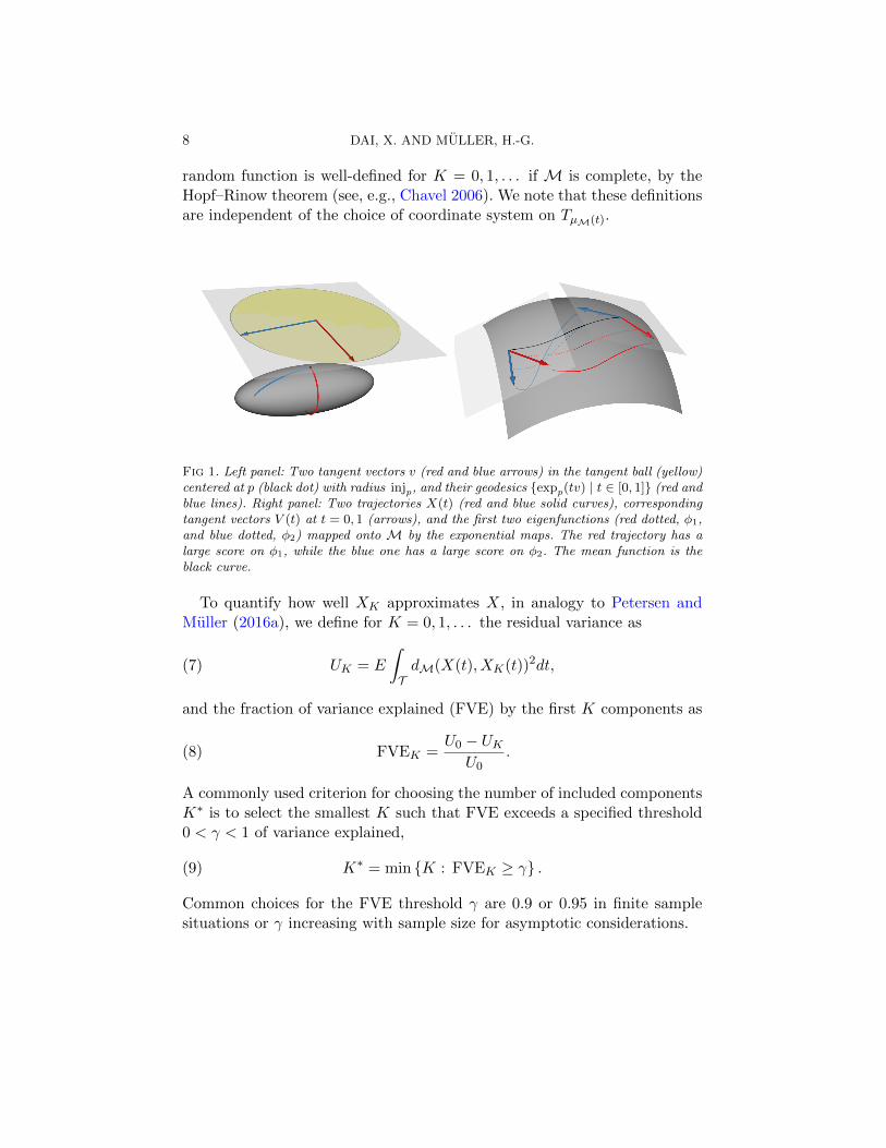
locally length minimizing curve. The exponential map at p ∈M is defined asexpp(v) = γv(1) where v ∈ TpM is a tangent vector at p, and γv is a uniquegeodesic with initial location γv(0) = p and velocity γ′v(0) = v. If (M, dM)is a complete metric space, then expp is defined on the entire tangent spaceTpM. The exponential map expp is a diffeomorphism in a neighborhood ofthe origin of the tangent space; the logarithm map logp is the inverse of expp.The radius of injectivity injp at p ∈M is the radius of the largest ball aboutthe origin of TpM, on which expp is a diffeomorphism (Figure 1, left panel).If N is a submanifold of M with Riemannian metric hp : TpN × TpN → R,(u, v) 7→ gp(u, v) for u, v ∈ TpN induced by g, then (N , h) is a Riemanniansubmanifold of (M, g).
We consider a d-dimensional complete Riemannian submanifold M of aEuclidean space Rd0 for d ≤ d0, with a geodesic distance dM onM inducedby the Euclidean metric in Rd0 , and a probability space (Ω,A, P ) with sam-ple space Ω, σ-algebra A, and probability measure P . With X = x : T →M | x ∈ C(T ) denoting the sample space of allM-valued continuous func-tions on a compact interval T ⊂ R and B(V) the Borel σ-algebra of a spaceV, the M-valued random functions X(t, ω) are X : T × Ω→M, such thatX(·, ω) ∈ X . Here ω 7→ X(·, ω) and X(t, ·) are measurable with respect toB(X ) and B(M), respectively, with B(X ) generated by the supremum met-ric dX : X × X → R, dX (x, y) = supt∈T dM(x(t), y(t)), for investigating therates of uniform convergence. In the following, all vectors v are column vec-tors and we write X(t), t ∈ T , forM-valued random functions, ‖·‖E for theEuclidean norm, and H = v : T → Rd0 ,
∫T v(t)T v(t)dt < ∞ for the am-
bient L2 Hilbert space of Rd0 valued square integrable functions, equippedwith the inner product 〈v, u〉 =
∫T v(t)Tu(t)dt and norm ‖v‖ = 〈v, v〉1/2 for
u, v ∈ H.
2.2. Riemannian functional principal component analysis. As intrinsicpopulation mean function for theM-valued random function X(t), we con-sider the intrinsic Frechet mean µM(t) at each time point t ∈ T , where
(1) M(p, t) = E[dM(X(t), p)2], µM(t) = arg minp∈M
M(p, t),
and we assume the existence and the uniqueness of the Frechet meansµM(t). The mean function µM is continuous due to the continuity of thesample paths of X, as per Proposition 2 below. One could consider analternative definition for the mean function, µG = arg minµ F (µ), whereF (µ) = E[
∫T dM(X(t), µ(t))2dt], which coincides with µM under a conti-
nuity assumption; we work with µM in (1), as it matches the approach infunctional PCA and allows us to investigate uniform convergence. The goal
6 DAI, X. AND MULLER, H.-G.
of RFPCA is to represent the variation of the infinite dimensional object Xaround the mean function µM in a lower dimensional submanifold, in termsof a few principal modes of variation, an approach that has been successfulto represent random trajectories in the Hilbert space L2 (Castro, Lawtonand Sylvestre 1986; Ramsay and Silverman 2005; Wang, Chiou and Muller2016).
Given an arbitrary system of K orthonormal basis functions, ΨK = ψk ∈H | ψk(t) ∈ TµM(t), 〈ψk, ψl〉 = δkl, k, l = 1, . . . ,K, δkl = 1 if k = l and 0otherwise, with values at each time t ∈ T restricted to the d-dimensionaltangent space TµM(t), which we identify with Rd0 for convenience, we definethe K dimensional time-varying geodesic submanifold(2)
MK(ΨK) := x ∈ X , x(t) = expµM(t)(K∑k=1
akψk(t)) for t ∈ T | ak ∈ R.
Here MK(ΨK) plays an analogous role to the linear span of a set of basisfunctions in Hilbert space, with expansion coefficients or coordinates ak.
In the following we suppress the dependency ofMK on the basis functions.With projections Π(x,MK) of an M-valued function x ∈ X onto time-varying geodesic submanifolds MK ,
Π(x,MK) := arg miny∈MK
∫TdM(y(t), x(t))2dt,
the best K-dimensional approximation to X minimizing the geodesic pro-jection distance is the geodesic submanifold that minimizes
(3) FS(MK) = E
∫TdM(X(t),Π(X,MK)(t))2dt
over all time-varying geodesic submanifolds generated by K basis functions.As the minimization of (3) is over a family of submanifolds (or basis
functions), this target is difficult to implement in practice, except for simplesituations, and therefore it is expedient to target a modified version of (3)by invoking tangent space approximations. This approximation requires thatthe log-mapped random functions
V (t) = logµM(t)(X(t))
are almost surely well-defined for all t ∈ T , which will be the case if trajec-tories X(t) are confined to stay within the radius of injectivity at µM(t) forall t ∈ T . We require this constraint to be satisfied, which will be the case

FUNCTIONAL DATA ON RIEMANNIAN MANIFOLDS 7
for many manifold-valued trajectory data, including the data we present inSection 5. Then V is a well-defined random function that assumes its valueson the linear tangent space TµM(t) at time t. Identifying TµM(t) with Rd0 ,
we may regard V as a random element of H, the L2 Hilbert space of Rd0valued square integrable functions, and thus our analysis is independent ofthe choice of the coordinate systems on the tangent spaces. A practicallytractable optimality criterion to obtain manifold principal components isthen to minimize
(4) FV (VK) = E(‖V −Π(V,VK)‖2)
over all K-dimensional linear subspaces VK(ψ1, . . . , ψK) = ∑K
k=1 akψk |ak ∈ R for ψk ∈ H, ψk(t) ∈ TµM(t), and k = 1, . . . ,K. Minimizing (4)is immediately seen to be equivalent to a multivariate functional principalcomponent analysis (FPCA) in Rd0 (Chiou, Chen and Yang 2014).
Under mild assumptions, the L2 mean function for the log-mapped dataV (t) = logµM(t)(X(t)) at the Frechet means is zero by Theorem 2.1 ofBhattacharya and Patrangenaru (2003). Consider the covariance functionG of V in the L2 sense, G : T × T → Rd20 , G(t, s) = cov(V (t), V (s)) =E(V (t)V (s)T ), and its associated spectral decomposition,G(t, s) =
∑∞k=1 λkφk(t)φk(s)
T , where the φk ∈ H : T → Rd0 are the or-thonormal vector-valued eigenfunctions and λk ≥ 0 the corresponding eigen-values, for k = 1, 2, . . . . One obtains the Karhunen-Loeve decomposition (seefor example Hsing and Eubank 2015),
(5) V (t) =
∞∑k=1
ξkφk(t),
where ξk =∫T V (t)φk(t)dt is the kth Riemannian functional principal com-
ponent (RFPC) score, k = 1, 2, . . . . A graphical demonstration of X(t),V (t), and φk(t) is in the right panel of Figure 1. In practice, one can useonly a finite number of components and target truncated representations ofthe tangent space process. Employing K ∈ 0, 1, 2, . . . components, set
(6) VK(t) =
K∑k=1
ξkφk(t), XK(t) = expµM(t)
(K∑k=1
ξkφk(t)
),
where for K = 0 the values of the sums are set to 0, so that V0(t) = 0 andX0(t) = µM(t). By classical FPCA theory, VK is the best K-dimensionalapproximation to V in the sense of being the minimizing projection Π(V,VK)for (4). The truncated representation XK(t), t ∈ T of the originalM-valued
8 DAI, X. AND MULLER, H.-G.
random function is well-defined for K = 0, 1, . . . if M is complete, by theHopf–Rinow theorem (see, e.g., Chavel 2006). We note that these definitionsare independent of the choice of coordinate system on TµM(t).
Fig 1. Left panel: Two tangent vectors v (red and blue arrows) in the tangent ball (yellow)centered at p (black dot) with radius injp, and their geodesics expp(tv) | t ∈ [0, 1] (red andblue lines). Right panel: Two trajectories X(t) (red and blue solid curves), correspondingtangent vectors V (t) at t = 0, 1 (arrows), and the first two eigenfunctions (red dotted, φ1,and blue dotted, φ2) mapped onto M by the exponential maps. The red trajectory has alarge score on φ1, while the blue one has a large score on φ2. The mean function is theblack curve.
To quantify how well XK approximates X, in analogy to Petersen andMuller (2016a), we define for K = 0, 1, . . . the residual variance as
(7) UK = E
∫TdM(X(t), XK(t))2dt,
and the fraction of variance explained (FVE) by the first K components as
(8) FVEK =U0 − UK
U0.
A commonly used criterion for choosing the number of included componentsK∗ is to select the smallest K such that FVE exceeds a specified threshold0 < γ < 1 of variance explained,
(9) K∗ = min K : FVEK ≥ γ .
Common choices for the FVE threshold γ are 0.9 or 0.95 in finite samplesituations or γ increasing with sample size for asymptotic considerations.
FUNCTIONAL DATA ON RIEMANNIAN MANIFOLDS 9
2.3. Spherical functional principal component analysis. An importantspecial case occurs when random trajectories lie on M = Sd, the Euclideansphere in Rd0 for d0 = d + 1, with the Riemannian geometry induced bythe Euclidean metric of the ambient space. Then the proposed RFPCA spe-cializes to spherical functional principal component analysis (SFPCA). Webriefly review the geometry of Euclidean spheres. The geodesic distance dMon the sphere is the great-circle distance, i.e. for p1, p2 ∈M = Sd
dM(p1, p2) = cos−1(p1T p2).
A geodesic is a segment of a great circle that connects two points onthe sphere. For any point p ∈ M, the tangent space TpM is identified byv ∈ Rd0 | vT p = 0 ⊂ Rd0 , with the Euclidean inner product. Letting‖·‖E be the Euclidean norm in the ambient Euclidean space Rd0 , then for atangent vector v on the tangent space TpM, the exponential map is
expp(v) = cos(‖v‖E)p+ sin(‖v‖E)v
‖v‖E.
The logarithm map logp :M\−p → TpM is the inverse of the exponentialmap,
logp(q) =u
‖u‖EdM(p, q),
where u = q− (pT q) p, and logp is defined everywhere with the exception ofthe antipodal point −p of p on M. The radius of injectivity is therefore π.The sectional curvature of a Euclidean sphere is constant.
2.4. Estimation. Consider a Riemannian manifold M and n indepen-dent observations X1, . . . , Xn, which are M-valued random functions thatare distributed as X, where we assume that these functions are fully ob-served for t ∈ T . Population quantities for RFPCA are estimated by theirempirical versions, as follows. Sample Frechet means µM(t) are obtained byminimizing Mn(·, t) at each t ∈ T ,
(10) Mn(p, t) =1
n
n∑i=1
dM(Xi(t), p)2, µM(t) = arg min
p∈MMn(p, t).
We estimate the log-mapped data Vi by Vi(t) = logµM(t)(Xi(t)), t ∈ T ;
the covariance function G(t, s) by the sample covariance function G(t, s) =n−1
∑ni=1 Vi(t)Vi(s)
T based on Vi, for t, s ∈ T ; the kth eigenvalue and eigen-
function pair (λk, φk) of G by the eigenvalue and eigenfunction (λk, φk) ofG; and the kth RFPC score of the ith subject ξik =
∫T Vi(t)φk(t)dt by

10 DAI, X. AND MULLER, H.-G.
ξik =∫T Vi(t)φk(t)dt. The K-truncated processes ViK and XiK for the ith
subject Xi are estimated by
(11) ViK(t) =
K∑k=1
ξikφk(t), XiK(t) = expµM(t)
(K∑k=1
ξikφk(t)
),
where again for K = 0 we set the sums to 0. The residual variance UK asin (7), the fraction of variance explained FVEK as in (8), and the optimalK∗ as in (9) are respectively estimated by
UK =1
n
n∑i=1
∫TdM(Xi(t), XiK(t))2dt,(12)
FVEK =U0 − UK
U0
,(13)
K∗ = minK : FVEK ≥ γ.(14)
Further details about the algorithms for implementing SFPCA can befound in the Supplementary Materials. Sometimes functional data X(t) areobserved only at densely spaced time points and observations might be con-taminated with measurement errors. In these situations one can presmooththe observations using smoothers that are adapted to a Riemannian mani-fold (Jupp and Kent 1987; Lin et al. 2016), treating the presmoothed curvesas fully observed underlying curves.
3. Theoretical properties of Riemannian Functional PrincipalComponent Analysis. We need the following assumptions (A1)–(A2) forthe Riemannian manifoldM, and (B1)–(B6) for theM-valued process X(t).
(A1) M is a closed Riemannian submanifold of a Euclidean space Rd0 , withgeodesic distance dM induced by the Euclidean metric.
(A2) The sectional curvature of M is nonnegative.
Assumption (A1) guarantees that the exponential map is defined on theentire tangent plane, so that XK(t) as in (6) is well-defined, while the cur-vature condition (A2) bounds the departure between XK(t) and X(t) bythat of their tangent vectors. These assumptions are satisfied for exampleby Euclidean spheres Sd. For the following recall M(p, t) and Mn(p, t) aredefined as in (1) and (10).
(B1) Trajectories X(t) are continuous for t ∈ T almost surely.(B2) For all t ∈ T , µM(t) and µM(t) exist and are unique, the latter almost
surely.
FUNCTIONAL DATA ON RIEMANNIAN MANIFOLDS 11
(B3) Almost surely, trajectoriesX(t) lie in a compact set St ⊂ BM(µM(t), r)for t ∈ T , where BM(µM(t), r) ⊂M is an open ball centered at µM(t)with radius r < inft∈T injµM(t).
(B4) For any ε > 0,
inft∈T
infp: dM(p,µM(t))>ε
M(p, t)−M(µM(t), t) > 0.
(B5) For v ∈ TµM(t)M, define gt(v) = M(expµM(t)(v), t). Then
inft∈T
λmin(∂2
∂v2gt(0)) > 0,
where λmin(A) is the smallest eigenvalue of a square matrix A.(B6) Let L(x) be the Lipschitz constant of a function x, i.e. L(x) =
supt6=s dM(x(t), x(s))/|t− s|. Then E(L(X)2) <∞ and L(µM) <∞.
Smoothness assumptions (B1) and (B6) for the sample paths of the ob-servations are needed for continuous representations, while existence anduniqueness of Frechet means (B2) are prerequisites for an intrinsic analy-sis that are commonly assumed (Bhattacharya and Patrangenaru 2003; Pe-tersen and Muller 2016b) and depend in a complex way on the type of mani-fold and probability measure considered. Assumptions (B4) and(B5) charac-terize the local behavior of the criterion function M around the minima andare standard for M-estimators (Bhattacharya and Lin 2017). Condition (B3)ensures that the geodesic between X(t) and µM(t) is unique, ensuring thatthe tangent vectors do not switch directions under small perturbations of thebase point µM(t). It is satisfied for example for the sphereM = Sd, if the val-ues of the random functions are either restricted to the positive quadrant ofthe sphere, as is the case for longitudinal compositional data as in Section 4,or if the samples are generated by expµM(t)(
∑∞k=1 ξkφk(t)) with bounded
eigenfunctions φk and small scores ξk such that supt∈T |∑∞
k=1 ξkφk(t)| ≤ r.In real data applications,(B3) is justified when theM-valued samples clusteraround the intrinsic mean function, as exemplified by the flight trajectorydata that we study in Subsection 5.2.
The following result justifies the tangent space RFPCA approach, as thetruncated representation is found to be well-defined, and the residual vari-ance for the optimal geodesic submanifold representation bounded by thatfor the classical FPCA on the tangent space.
Proposition 1. Under (A1), XK(t) = expµM(t)(VK(t)) is well-defined
12 DAI, X. AND MULLER, H.-G.
for K = 1, 2, . . . and t ∈ T . If further (A2) is satisfied, then(15)
minMK
∫TdM(X(t),Π(X,MK)(t))2dt ≤
∫TdM(X(t), XK(t))2dt ≤ ‖V − VK‖2 .
The first statement is a straightforward consequence of the Hopf-Rinowtheorem, while the inequalities imply that the residual variance using thebest K-dimensional time-varying geodesic manifold approximation undergeodesic distance (the left hand term) is bounded by that of the geodesicmanifold produced by the proposed RFPCA (the middle term), where thelatter is again bounded by the residual variance of a linear tangent spaceFPCA under the familiar Euclidean distance (the right hand term). Ther.h.s. inequality in (15) affirms that the tangent space FPCA serves as agauge to control the preciseness of finite-dimensional approximation to theprocesses under the geodesic distance. An immediate consequence is thatUK → 0 as K → ∞ for the residual variance UK in (7), implying thatthe truncated representation XK(t) is consistent for X(t) when the sec-tional curvature of M is nonnegative. The l.h.s. inequality gets tighter asthe samples X(t) lie closer to the intrinsic mean µM(t), where such closenessis not uncommon, as demonstrated in Section 5. The r.h.s. inequality is aconsequence of the Alexandrov–Toponogov theorem for comparing geodesictriangles.
Asymptotic properties for the estimated model components for RFPCAare studied below.
Proposition 2. Under (A1) and (B1)– (B4), µM(t) is continuous,µM(t) is continuous with probability tending to 1 as n→∞, and
(16) supt∈T
dM(µM(t), µM(t)) = op(1).
Under additional assumptions (B5) and (B6), the consistency in (16)of the sample intrinsic mean µM(t) as an estimator for the true intrin-sic mean µM(t) can be strengthened through a central limit theorem onCd(T ), where Cd(T ) is the space of Rd-valued continuous functions on T .Let τ : U → Rd be a smooth or infinitely differentiable chart of the formτ(q) = logp0(q), with U = BM(p0, r0), p0 ∈ M, and r0 < injp0 , identi-
fying tangent vectors in Rd. Define chart distance dτ : τ(U) × τ(U) → Rby dτ (u, v) = dM(τ−1(u), τ−1(v)), its gradient T (u, v) = [Tj(u, v)]dj=1 =
[∂dτ (u, v)/∂vj ]dj=1, Hessian matrix H(u, v) with (j, l)th element Hjl(u, v) =
∂2d2τ (u, v)/∂vj∂vl, and Λ(t) = E[H(τ(X(t)), τ(µM(t)))].
FUNCTIONAL DATA ON RIEMANNIAN MANIFOLDS 13
Theorem 1. Suppose that µM(t) and X(t) are contained in the domainof τ for t ∈ T , the latter almost surely, and (A1) and (B1)–(B6) hold. Then
(17)√n[τ(µM)− τ(µM)]
L−→ Z,
where Z is a Gaussian process with sample paths in Cd(T ), mean zero, andcovariance Gµ(t, s) = Λ−1(t)GT (t, s)Λ−1(s), whereGT (t, s) = E[T (τ(X(t)), τ(µM(t)))T (τ(X(s)), τ(µM(s)))T ], and all quanti-ties are well-defined.
Remark 1. The first condition in Theorem 1 is not restrictive, since itholds at least piecewise on some finite partition of T . More precisely, due tothe compactness guaranteed by (A1), (B3), and Proposition 2, there existsa finite partition TjNj=1 of T such that µM(t) and X(t) are contained inBM(µM(tj), rj), for t ∈ Tj , tj ∈ M and rj < injµM(tj), j = 1, . . . , N < ∞.One can then define τ = τj := q 7→ logµM(tj)(q) for t ∈ Tj and applyTheorem 1 on the jth piece, for each j.
Corollary 1. Under (A1) and (B1)–(B6),
(18) supt∈T
dM(µM(t), µM(t)) = Op(n−1/2).
Remark 2. The intrinsic dimension d is only reflected in the rate con-stant but not the speed of convergence. Our situation is analogous to thatof estimating the mean of Euclidean-valued random functions (Bosq 2000),or more generally, Frechet regression with Euclidean responses (Petersenand Muller 2016b), where the speed of convergence does not depend on thedimension of the Euclidean space, in contrast to common nonparametricregression settings (Lin et al. 2016; Lin and Yao 2017). The root-n rate isnot improvable in general since it is the optimal rate for mean estimates inthe special Euclidean case.
An immediate consequence of Corollary 1 is the convergence of the log-mapped data.
Corollary 2. Under (A1) and (B1)–(B6), for i = 1, . . . , n,
(19) supt∈T‖Vi(t)− Vi(t)‖E = Op(n
−1/2).
In the following, we use the Frobenius norm ‖A‖F = tr(ATA)1/2 for anyreal matrices A, and assume that the eigenspaces associated with positive
14 DAI, X. AND MULLER, H.-G.
eigenvalues λk > 0 have multiplicity one. We obtain convergence of covari-ance functions, eigenvalues, and eigenfunctions on the tangent spaces, i.e.,the consistency of the spectral decomposition of the sample covariance func-tion, as follows.
Theorem 2. Assume (A1) and (B1)–(B6) hold. Then
supt,s∈T
∥∥∥G(t, s)−G(t, s)∥∥∥F
= Op(n−1/2),(20)
supk∈N|λk − λk| = Op(n
−1/2),(21)
and for each k = 1, 2, . . . with λk > 0,
supt∈T‖φk(t)− φk(t)‖E = Op(n
−1/2).(22)
Our next result provides the convergence rate of the RFPC scores and isa direct consequence of Corollary 2 and Theorem 2.
Theorem 3. Under (A1) and (B1)–(B6), if λK > 0 for some K ≥ 1,then for each i = 1, . . . , n and k = 1, . . . ,K,
|ξik − ξik| = Op(n−1/2),(23)
supt∈T‖ViK(t)− ViK(t)‖E = Op(n
−1/2).(24)
To demonstrate asymptotic consistency for the number of componentsselected according to the FVE criterion, we consider an increasing sequenceof FVE thresholds γ = γn ↑ 1 as sample size n increases, which leads to acorresponding increasing sequence of K∗ = K∗n, where K∗ is the smallestnumber of eigen-components that explains the fraction of variance γ = γn.One may show that the number of components K∗ selected from the sampleis consistent for the true target K∗ for a sequence γn. This is formalizedin the following Corollary 3, which is similar to Theorem 2 in Petersenand Muller (2016a), where also specific choices of γn and the correspond-ing sequences K∗ were discussed. The proof is therefore omitted. Quanti-ties U0, UK , K
∗, U0, UK , K∗ that appear below were defined in (7)–(9) and
(12)–(14).
Corollary 3. Assume (A1)–(A2) and (B1)–(B6) hold. If the eigenval-ues λ1 > λ2 > · · · > 0 are all distinct, then there exists a sequence 0 < γn ↑ 1such that
(25) max1≤K≤K∗
∣∣∣∣∣ U0 − UKU0
− U0 − UKU0
∣∣∣∣∣ = op(1),
FUNCTIONAL DATA ON RIEMANNIAN MANIFOLDS 15
and therefore
(26) P (K∗ 6= K∗) = o(1).
4. Longitudinal compositional data analysis. Compositional datarepresent proportions and are characterized by a vector y in the simplex
CJ−1 = y = [y1, . . . , yJ ] ∈ RJ | yj ≥ 0, j = 1, . . . , J ;
J∑j=1
yj = 1,
requiring that the nonnegative proportions of all J categories sum up to one.Typical examples include the geochemical composition of rocks or other datathat consist of recorded percentages. Longitudinal compositional data arisewhen the compositional data for the same subject are collected repeatedlyat different time points. If compositions are monitored continuously, eachsample path of longitudinal compositional data is a function y : T → CJ−1.Analyses of such data, for example from a prospective ophthalmology study(Qiu, Song and Tan 2008) or the surveillance of the composition of antimicro-bial use over time (Adriaenssens et al. 2011), have drawn both methodologi-cal and practical interest, but as of yet there exists no unifying methodologyfor longitudinal compositional data, to the knowledge of the authors.
A direct application of standard Euclidean space methods, viewing longi-tudinal compositional data as unconstrained functional data vectors (Chiou,Chen and Yang 2014), would ignore the non-negativity and unit sum con-straints and therefore the resulting multivariate FPCA representation movesoutside of the space of compositional data, diminishing the utility of suchsimplistic approaches. There are various transformation that have been pro-posed over the years for the analysis of compositional data to enforce theconstraints, for example log-ratio transformations such as log(yj/yJ) forj = 1, . . . , J − 1, after which the data are treated as Euclidean data (Aitchi-son 1986), which induces the Aitchison geometry on the interior of the sim-plex CJ−1. However, these transformations cannot be defined when some ofthe elements in the composition are zeros, either due to the discrete andnoisy nature of the observations or when the true proportions do containactual zeros, as is the case in the fruit fly behavior pattern data that westudy in Subsection 5.1 below.
We propose to view longitudinal compositional data as a special case ofmultivariate functional data under constraints, specifically as realizations of
16 DAI, X. AND MULLER, H.-G.
a compositional process over time,(27)
Y (t) ∈ [Y1(t), . . . , YJ(t)] ∈ RJ | Yj ∈ L2(T ), Yj(t) ≥ 0,J∑j=1
Yj(t) = 1,
where the component functions will also be assumed to be continuous ontheir domain T . To include the entire simplex CJ−1 in our longitudinalcompositional data analysis, we apply square root transformations to thelongitudinal compositional data Y (t) = [Y1(t), . . . , YJ(t)], obtaining
(28) X(t) = [X1(t), . . . , XJ(t)] = [Y1(t)1/2, . . . , YJ(t)1/2].
A key observation is that the values of X(t) lie on the positive quadrant ofa hypersphere SJ−1 for t ∈ T , as Xj(t) ≥ 0 and
∑Jj=1Xj(t)
2 = 1. Thereis no problem with zeros as with some other proposed transformations forcompositional data. It is then a natural approach to consider a spherical ge-ometry for the transformed data X(t). A square-root transformation and thespherical geometry for non-longitudinal compositional data were previouslyconsidered by Huckemann and Eltzner (2016). Now, since X(t) assumes itsvalues on a quadrant of the sphere SJ−1, processes X(t) fall into the frame-work of the proposed SFPCA, as described in Subsection 2.3.
Concerning the theoretical properties of SFPCA of longitudinal compo-sitional data, the conditions on the Riemannian manifold M needed forRFPCA are easily seen to be satisfied, due to the geometry of the Euclideansphere and the positive quadrant constraint. We conclude
Corollary 4. Under (B1) and (B4)–(B6), Propositions 1 and 2, The-orems 1–3, and Corollaries 1–3 hold for the Spherical Functional PrincipalComponent Analysis (SFPCA) of longitudinal compositional data X(t) in(28).
5. Data applications.
5.1. Fruit fly behaviors. To illustrate the proposed SFPCA based longi-tudinal compositional data analysis, we consider the lifetime behavior pat-tern data of D. melanogaster (common fruit fly, Carey et al. 2006). The be-havioral patterns of each fruit fly was observed instantaneously 12 times eachday during its entire lifetime, and for each observation one of the five behav-ioral patterns, feeding, flying, resting, walking, and preening, was recorded.We analyzed the behavioral patterns in the first 30 days since eclosion forn = 106 fruit flies with uncensored observations, aiming to characterize and
FUNCTIONAL DATA ON RIEMANNIAN MANIFOLDS 17
represent age-specific behavioral patterns of individual fruit flies. For eachfruit fly, we observed the behavioral counts [Z1(t), . . . , Z5(t)] for the five be-haviors at time t ∈ T = [0, 30], where the time unit is day since eclosion,and
∑5j=1 Zj(t) = 12 is the constrained total number of counts at each time
t, with 0 ≤ Zj(t) ≤ 12 for each j and t. Since the day-to-day behavioraldata are noisy, we presmoothed the counts Zj(t) of the jth behavior pat-tern over time for j = 1, . . . , 5, using a Nadaraya–Watson kernel smoother(Nadaraya 1964; Watson 1964) with Epanechnikov kernel and a bandwidthof five days. The smoothed data were subsequently divided by the sumof the smoothed component values at each t, yielding a functional vectorY (t) = [Y1(t), . . . , Y5(t)], with Yj(t) ≥ 0 for all j and t and
∑5j=1 Yj(t) = 1
for t ∈ T , thus corresponding to longitudinal compositional data.Following the approach described in Section 4, we model the square-root
composition proportions X(t) = [Y1(t)1/2, . . . , Y5(t)
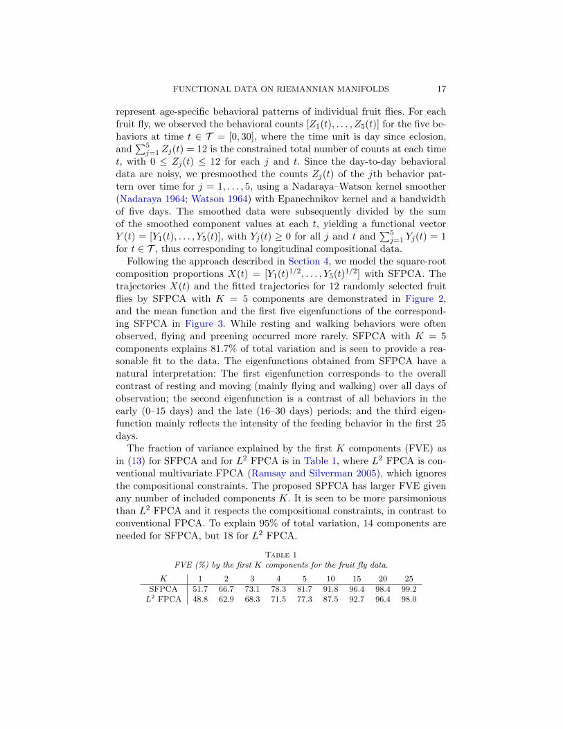
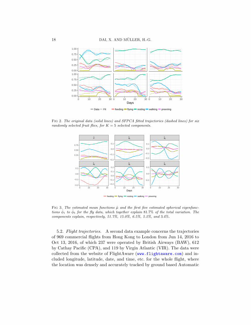
1/2] with SFPCA. Thetrajectories X(t) and the fitted trajectories for 12 randomly selected fruitflies by SFPCA with K = 5 components are demonstrated in Figure 2,and the mean function and the first five eigenfunctions of the correspond-ing SFPCA in Figure 3. While resting and walking behaviors were oftenobserved, flying and preening occurred more rarely. SFPCA with K = 5components explains 81.7% of total variation and is seen to provide a rea-sonable fit to the data. The eigenfunctions obtained from SFPCA have anatural interpretation: The first eigenfunction corresponds to the overallcontrast of resting and moving (mainly flying and walking) over all days ofobservation; the second eigenfunction is a contrast of all behaviors in theearly (0–15 days) and the late (16–30 days) periods; and the third eigen-function mainly reflects the intensity of the feeding behavior in the first 25days.
The fraction of variance explained by the first K components (FVE) asin (13) for SFPCA and for L2 FPCA is in Table 1, where L2 FPCA is con-ventional multivariate FPCA (Ramsay and Silverman 2005), which ignoresthe compositional constraints. The proposed SPFCA has larger FVE givenany number of included components K. It is seen to be more parsimoniousthan L2 FPCA and it respects the compositional constraints, in contrast toconventional FPCA. To explain 95% of total variation, 14 components areneeded for SFPCA, but 18 for L2 FPCA.
Table 1FVE (%) by the first K components for the fruit fly data.
K 1 2 3 4 5 10 15 20 25
SFPCA 51.7 66.7 73.1 78.3 81.7 91.8 96.4 98.4 99.2L2 FPCA 48.8 62.9 68.3 71.5 77.3 87.5 92.7 96.4 98.0
18 DAI, X. AND MULLER, H.-G.
0 10 20 30 0 10 20 30 0 10 20 30
0.00
0.25
0.50
0.75
1.00
0.00
0.25
0.50
0.75
1.00
0.00
0.25
0.50
0.75
1.00
0.00
0.25
0.50
0.75
1.00
Days
Data Fit feeding flying resting walking preening
Fig 2. The original data (solid lines) and SFPCA fitted trajectories (dashed lines) for sixrandomly selected fruit flies, for K = 5 selected components.
φ3 φ4 φ5
µ φ1 φ2
0 10 20 30 0 10 20 30 0 10 20 30
−0.2
−0.1
0.0
0.1
−0.2
0.0
0.2
−0.2
−0.1
0.0
0.1
−0.2
−0.1
0.0
0.1
0.2
0.25
0.50
0.75
−0.2
−0.1
0.0
0.1
Days
feeding flying resting walking preening
Fig 3. The estimated mean functions µ and the first five estimated spherical eigenfunc-tions φ1 to φ5 for the fly data, which together explain 81.7% of the total variation. Thecomponents explain, respectively, 51.7%, 15.0%, 6.5%, 5.2%, and 3.4%.
5.2. Flight trajectories. A second data example concerns the trajectoriesof 969 commercial flights from Hong Kong to London from Jun 14, 2016 toOct 13, 2016, of which 237 were operated by British Airways (BAW), 612by Cathay Pacific (CPA), and 119 by Virgin Atlantic (VIR). The data werecollected from the website of FlightAware (www.flightaware.com) and in-cluded longitude, latitude, date, and time, etc. for the whole flight, wherethe location was densely and accurately tracked by ground based Automatic
FUNCTIONAL DATA ON RIEMANNIAN MANIFOLDS 19
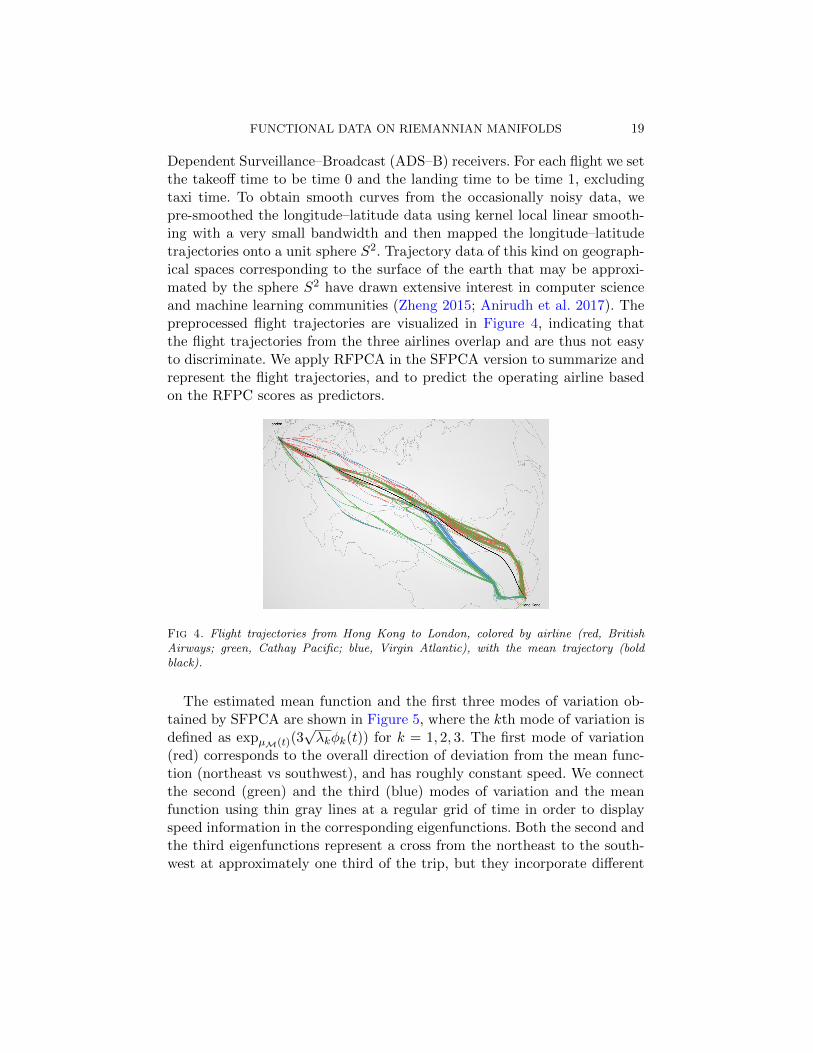
Dependent Surveillance–Broadcast (ADS–B) receivers. For each flight we setthe takeoff time to be time 0 and the landing time to be time 1, excludingtaxi time. To obtain smooth curves from the occasionally noisy data, wepre-smoothed the longitude–latitude data using kernel local linear smooth-ing with a very small bandwidth and then mapped the longitude–latitudetrajectories onto a unit sphere S2. Trajectory data of this kind on geograph-ical spaces corresponding to the surface of the earth that may be approxi-mated by the sphere S2 have drawn extensive interest in computer scienceand machine learning communities (Zheng 2015; Anirudh et al. 2017). Thepreprocessed flight trajectories are visualized in Figure 4, indicating thatthe flight trajectories from the three airlines overlap and are thus not easyto discriminate. We apply RFPCA in the SFPCA version to summarize andrepresent the flight trajectories, and to predict the operating airline basedon the RFPC scores as predictors.
Fig 4. Flight trajectories from Hong Kong to London, colored by airline (red, BritishAirways; green, Cathay Pacific; blue, Virgin Atlantic), with the mean trajectory (boldblack).
The estimated mean function and the first three modes of variation ob-tained by SFPCA are shown in Figure 5, where the kth mode of variation isdefined as expµM(t)(3
√λkφk(t)) for k = 1, 2, 3. The first mode of variation
(red) corresponds to the overall direction of deviation from the mean func-tion (northeast vs southwest), and has roughly constant speed. We connectthe second (green) and the third (blue) modes of variation and the meanfunction using thin gray lines at a regular grid of time in order to displayspeed information in the corresponding eigenfunctions. Both the second andthe third eigenfunctions represent a cross from the northeast to the south-west at approximately one third of the trip, but they incorporate different

20 DAI, X. AND MULLER, H.-G.
speed information. The second eigenfunction encodes an overall fast tripstarting to the north, while the third encodes a medium speed start to thesouth and then a speed up after crossing to the north. The FVE for RFPCAusing the first K = 3 eigenfunctions is 95%, indicating a reasonably goodapproximation of the true trajectories.
Fig 5. The mean function (black) and the first three modes of variation defined asexpµM(t)(3
√λkφk(t)), k = 1, 2, 3 (red, green, and blue, respectively) produced by SFPCA.
The second and the third modes of variation were joined to the time-varying mean func-tion at a regular grid of time points to show the “speed” of the eigenfunctions. Both thesecond and the third eigenfunctions represent a cross from the northeast to the southwestat approximately one third of the trip, but they incorporate different speed information asshown by the thin gray lines. The first three eigenfunctions together explain in total 95%and each explain 72.9%, 13.2%, and 8.9%, respectively, of total variation.
We next compared the FVE by the SFPCA and the L2 FPCA forK = 1, . . . , 10 under the geodesic distance dM. Here the SFPCA was ap-plied on the spherical data on S2, while the L2 FPCA was based on thelatitude–longitude data in R2. A summary of the FVE for the SFPCA andthe L2 FPCA is shown in Table 2, using the first K = 1, . . . , 10 compo-nents. Again SFPCA has higher FVE than the conventional L2 FPCA forall choices of K, especially small K, where SFPCA shows somewhat betterperformance in terms of trajectory recovery.
Table 2The FVE (%) by the first K components for the proposed SFPCA and the L2 FPCA for
the flight data.
K 1 2 3 4 5 6 7 8 9 10
SFPCA 72.9 86.1 95.0 96.3 97.0 97.7 98.3 98.7 99.0 99.2L2 FPCA 71.2 84.9 94.6 96.1 96.8 97.4 98.1 98.4 98.8 99.1
We also aimed to predict the airline (BAW, CPA, and VIR) from an ob-
FUNCTIONAL DATA ON RIEMANNIAN MANIFOLDS 21
served flight path by feeding the FPC scores obtained from either the pro-posed SFPCA or from the traditional L2 FPCA into different multivariateclassifiers, including linear discriminant analysis (LDA), logistic regression,and support vector machine (SVM) with radial basis kernel. For each of200 Monte Carlo runs, we randomly selected 500 flights as training set fortraining and tuning and used the rest as test set to evaluate classificationperformance. The number of components K for each classifier was eitherfixed at 10, 15, 20, 25, 30, or selected by five-fold cross-validation (CV). Theresults for prediction accuracy are in Table 3. The SFPCA based classifiersperformed better or at least equally well as the L2 FPCA based classifiersfor nearly all choices of K and classifier, where among the classifiers SVMperformed best.
Table 3A comparison of airline classification accuracy (%) from observed flight trajectories,
using the first K components for SFPCA and L2 FPCA (columns), with K either fixedor chosen by CV, for various classifiers (rows). All standard errors for the accuracies arebelow 0.12%. The numbers in parenthesis are the number of components chosen by CV. S
stands for SFPCA and L for L2 FPCA; LDA, linear discriminant analysis; MN,multinomial logistic regression; SVM, support vector machine.
K = 10 K = 15 K = 20 K = 25 K = 30 K chosen by CVS L S L S L S L S L S L
LDA 76.9 75.8 79.6 78.4 81.9 81.5 82.7 82.5 83.5 82.3 83.2 (28.0) 82.2 (26.2)MN 78.5 76.0 81.8 79.4 83.8 82.7 84.6 84.0 85.2 83.6 84.8 (27.5) 83.7 (25.7)SVM 82.3 80.9 84.3 82.5 86.3 85.2 86.1 86.2 86.3 85.7 86.2 (24.6) 85.8 (25.0)
6. Simulations. To investigate the performance of trajectory recoveryfor the proposed RFPCA, we considered two scenarios of Riemannian mani-folds: The Euclidean sphereM = S2 in R3, and the special orthogonal groupM = SO(3) of 3 × 3 rotation matrices, viewed as a Riemannian submani-fold of R3×3. We compared three approaches: The Direct (D) method, whichdirectly optimizes (3) over all time-varying geodesic submanifolds MK andtherefore serves as a gold standard, implemented through discretization; theproposed RFPCA method (R) and the classical L2 FPCA method (L), whichignores the Riemannian geometry. In the direct method, the sample curvesand time-varying geodesic submanifolds are discretized onto a grid of 20equally-spaced time points, and a quasi-Newton algorithm is used to max-imize the criterion function (3). We used FVE as our evaluation criterion,where models were fitted using n = 50 or 100 independent samples.
We briefly review the Riemannian geometry for the special orthogonalgroup M = SO(N). The elements of M are N × N orthogonal matriceswith determinant 1, and the tangent space TpM is identified with the col-
22 DAI, X. AND MULLER, H.-G.
lection ofN×N skew-symmetric matrices. For p, q ∈M and skew-symmetricmatrices u, v ∈ TpM, the Riemannian metric is 〈u, v〉 = tr(uT v) where tr(·)is the matrix trace; the Riemannian exponential map is expp(v) = Exp(v)pand the logarithm map is logp(q) = Log(qp−1), where Exp and Log denotethe matrix exponential and logarithm; the geodesic distance is dM(p, q) =∥∥Log(qp−1)
∥∥F
. For N = 3, the tangent space TpM is 3-dimensional andcan be identified with R3 through (Chavel 2006) ι : R3 → TpM, ι(a, b, c) =[0,−a,−b; a, 0,−c; b, c, 0].
The sample curves X were generated as X : T = [0, 1]→M,X(t) = expµM(t)(
∑20k=1 ξkφk(t)), with mean function µM(t) =
exp[0,0,1](2t, 0.3π sin(πt), 0) forM = S2, and µM(t) = exp(ι(2t, 0.3π sin(πt), 0))forM = SO(3). For k = 1, . . . , 20, the RFPC scores ξk were generated by in-dependent Gaussian distributions with mean zero and variance 0.07k/2. Theeigenfunctions were φk(t) = 2−1/2Rt[ζk(t/2), ζk((t + 1)/2), 0]T for M = S2
and φk(t) = 6−1/2ι(ζk(t/3), ζk((t + 1)/3), ζk((t + 2)/3)) for M = SO(3),t ∈ [0, 1], where Rt is the rotation matrix from [0, 0, 1] to µM(t), and ζk20k=1
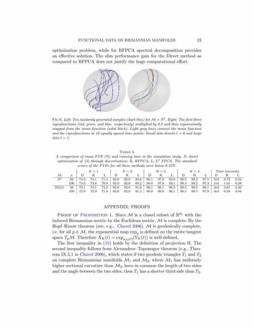
is the orthonormal Legendre polynomial basis on [0, 1]. A demonstration often sample curves, the mean function, and the first three eigenfunctions forM = S2 is shown in Figure 6.
We report the mean FVE by the first K = 1, . . . , 4 components for theinvestigated FPCA methods in Table 4, as well as the running time, basedon 200 Monte Carlo repeats. The true FVEs for K = 1, . . . , 4 componentswere 73.5%, 93.0%, 98.1%, and 99.5%, respectively. The proposed RFPCAmethod had higher FVE and thus outperformed the L2 FPCA in all scenariosand for all K, which is expected since RFPCA takes into account the curvedgeometry. This advantage leads to a more parsimonious representation, e.g.,in the M = S2 and n = 100 scenario, the average K required by RFPCAto achieve at least FVE> 0.95 is one less than that for L2 FPCA. Theperformance advantage of RFPCA over L2 FPCA is larger for M = S2
than for M = SO(3), since the former has larger sectional curvature (1vs 1/8). The Direct method was as expected better than RFPCA (also forSO(3), which is not explicit in the table due to rounding), since the formeroptimizes the residual variation under the geodesic distance, the true target,while the latter uses the more tractable surrogate residual variation target(4) for L2 distance on the tangent spaces.
Each experiment was run using a single processor (Intel Xeon E5-2670CPU @ 2.60GHz) to facilitate comparisons. Both RFPCA and L2 FPCA arequite fast in the and take only a few seconds, though RFPCA is 1.5–3 timesslower, depending on the Riemannian manifoldM. The Direct method, how-ever, was several magnitudes slower than RFPCA, due to the unstructured
FUNCTIONAL DATA ON RIEMANNIAN MANIFOLDS 23
optimization problem, while for RFPCA spectral decomposition providesan effective solution. The slim performance gain for the Direct method ascompared to RFPCA does not justify the huge computational effort.
Fig 6. Left: Ten randomly generated samples (dark blue) forM = S2. Right: The first threeeigenfunctions (red, green, and blue, respectively) multiplied by 0.2 and then exponentiallymapped from the mean function (solid black). Light gray lines connect the mean functionand the eigenfunctions at 10 equally spaced time points. Small dots denote t = 0 and largedots t = 1.
Table 4A comparison of mean FVE (%) and running time in the simulation study. D, directoptimization of (3) through discretization; R, RFPCA; L, L2 FPCA. The standard
errors of the FVEs for all three methods were below 0.32%.
K = 1 K = 2 K = 3 K = 4 Time (seconds)M n D R L D R L D R L D R L D R LS2 50 74.3 74.1 71.4 93.0 92.9 89.6 98.1 97.9 93.8 99.5 99.2 97.5 5e3 0.72 0.24
100 74.0 73.8 70.9 92.9 92.8 89.2 98.0 97.9 93.1 99.4 99.2 97.3 1e4 1.01 0.38SO(3) 50 73.1 73.1 72.2 92.8 92.8 91.6 98.1 98.1 96.3 99.5 99.5 98.1 2e3 3.67 2.46
100 72.9 72.9 71.8 92.6 92.6 91.3 98.0 98.0 96.1 99.5 99.5 97.9 4e3 6.58 4.94
APPENDIX: PROOFS
Proof of Proposition 1. Since M is a closed subset of Rd0 with theinduced Riemannian metric by the Euclidean metric,M is complete. By theHopf–Rinow theorem (see, e.g., Chavel 2006), M is geodesically complete,i.e. for all p ∈M, the exponential map expp is defined on the entire tangentspace TpM. Therefore XK(t) = expµM(t)(VK(t)) is well-defined.
The first inequality in (15) holds by the definition of projection Π. Thesecond inequality follows from Alexandrov–Toponogov theorem (e.g., Theo-rem IX.5.1 in Chavel 2006), which states if two geodesic triangles T1 and T2on complete Riemannian manifolds M1 and M2, where M1 has uniformlyhigher sectional curvature thanM2, have in common the length of two sidesand the angle between the two sides, then T1 has a shorter third side than T2.
24 DAI, X. AND MULLER, H.-G.
This is applied to triangles (X(t), µM(t), XK(t)) onM and (V (t), 0, VK(t))on TµM(t), identified with a Euclidean space.
For the following proofs we consider the set
(29) K =⋃t∈T
BM(µM(t), 2r) ⊂M,
where BM(p, l) is an open dM-geodesic ball of radius l > 0 centered atp ∈M, and A denotes the closure of a set A. Under(B1) and(B3), K is closedand bounded and thus is compact, with diameter R = supp,q∈K dM(p, q).Then µM(t), µM(t), X(t) ∈ K for all t ∈ T . For the asymptotic results wewill consider the compact set K.
Proof of Proposition 2. To obtain the uniform consistency results ofµM(t), we need to show
supt∈T
supp∈K|Mn(p, t)−M(p, t)| = op(1),(30)
supt∈T|Mn(µM(t), t)−M(µM(t), t)| = op(1),(31)
and for any ε > 0, there exist a = a(ε) > 0 such that
(32) inft∈T
infp: dM(p,µM(t))>ε
[Mn(p, t)−M(µM(t), t)] ≥ a− op(1).
Then by (31) and (32), for any δ > 0, there exists N ∈ N such that n ≥ Nimplies the event
E = supt∈T|Mn(µM(t), t)−M(µM(t), t)| ≤ a/3∩ inf
t∈Tinf
p: dM(p,µM(t))>ε[Mn(p, t)−M(µM(t), t)] ≥ 2a/3
holds with probability greater than 1−δ. This implies that on E, supt∈T dM(µM(t), µM(t)) ≤ε, and therefore the consistency of µM.
Proof of (30): We first obtain the auxiliary result
(33) limδ↓0
E
[sup|t−s|<δ
dM(X(t), X(s))
]= 0
by dominated convergence, (B1), and the boundedness of K (29). Note thatfor any p, q, w ∈ K,
|dM(p, w)2−dM(q, w)2| = |dM(p, w)+dM(q, w)|·|dM(p, w)−dM(q, w)| ≤ 2RdM(p, q)
FUNCTIONAL DATA ON RIEMANNIAN MANIFOLDS 25
by the triangle inequality, where R is the diameter of K. Then
sup|t−s|<δp,q∈K
dM(p,q)<δ
|Mn(p, t)−Mn(q, s)| ≤ sup|t−s|<δp,q∈K
dM(p,q)<δ
|Mn(p, s)−Mn(q, s)|+ sup|t−s|<δp,q∈K
dM(p,q)<δ
|Mn(p, t)−Mn(p, s)|
≤ 2Rδ +2R
n
n∑i=1
sup|t−s|<δ
dM(Xi(t), Xi(s))
= 2Rδ + 2RE
[sup|t−s|<δ
dM(X(t), X(s))
]+ op(1),
where the last equality is due to the weak law of large numbers (WLLN).Due to (33), the quantity in the last display can be made arbitrarily close tozero (in probability) by letting δ ↓ 0 and n → ∞. Therefore, for any ε > 0and η > 0, there exist δ > 0 such that
lim supn→∞
P ( sup|t−s|<δp,q∈K
dM(p,q)<δ
|Mn(p, t)−Mn(q, s)| > ε) < η,
proving the asymptotic equicontinuity of Mn on K×T . This and the point-wise convergence ofMn(p, t) toM(p, t) by the WLLN imply (30) by Theorem1.5.4 and Theorem 1.5.7 of van der Vaart and Wellner (1996).
Proof of (31): Since µM(t) and µM(t) are the minimizers of Mn(·, t) andM(·, t), respectively, |Mn(µM(t), t) −M(µM(t), t)| ≤ max(Mn(µM(t), t) −M(µM(t), t),M(µM(t), t) − Mn(µM(t), t)) ≤ supp∈K |Mn(p, t) − M(p, t)|.Take suprema over t ∈ T and then apply (30) to obtain (31).
Proof of (32): Fix ε > 0 and let a = a(ε) = inft∈T infp: dM(p,µM(t))>ε[M(p, t)−M(µM(t), t)] > 0. For small enough ε,
inft∈T
infp: dM(p,µM(t))>ε
[Mn(p, t)−M(µM(t), t)] = inft∈T
infp∈K,
dM(p,µM(t))>ε
[Mn(p, t)−M(µM(t), t)]
= inft∈T
infp∈K,
dM(p,µM(t))>ε
[M(p, t)−M(µM(t), t) +Mn(p, t)−M(p, t)]
≥ a− supt∈T
supp∈K
dM(p,µM(t))>ε
|Mn(p, t)−M(p, t)| = a− op(1),
where the first equality is due to µM(t) ∈ K and the continuity of Mn, theinequality to (B4), and the last equality to (30). For the continuity of µM,note for any t0, t1 ∈ T ,
|M(µM(t1), t0)−M(µM(t0), t0)| ≤ |M(µM(t1), t1)−M(µM(t0), t0)|+ |M(µM(t1), t0)−M(µM(t1), t1)|
26 DAI, X. AND MULLER, H.-G.
≤ supp∈K|M(p, t1)−M(p, t0)|+ 2RE[dM(X(t0), X(t1))]
≤ 4RE[dM(X(t0), X(t1))]→ 0
as t1 → t0 by(B1), where the second inequality is due to the fact that µM(tl)minimizes M(·, tl) for l = 0, 1. Then by (B4), dM(µM(t1), µM(t0)) → 0 ast1 → t0, proving the continuity of µM. The continuity for µM is similarlyproven by in probability arguments.
Proof of Theorem 1. The proof idea is similar to that of Theorem 2.1in Bhattacharya and Patrangenaru (2005). To lighten notations, let Y (t) =τ(X(t)), Yi(t) = τ(Xi(t)), ν(t) = τ(µM(t)), and ν(t) = τ(µM(t)). Thesquared distance dM(p, q)2 is smooth at (p, q) if dM(p, q) < injp, due tothe smoothness of the exponential map (Chavel 2006, Theorem I.3.2). Thendτ (u, v)2 is smooth on the compact set (u, v) ∈ τ(U) × τ(U) ⊂ Rd × Rd |dM(τ−1(u), τ−1(v)) ≤ r and thus T (Y (t), ν(t)) and H(Y (t), ν(t)) are welldefined, by (B3) and since the domain U of τ is bounded. Define
ht(v) = E[dτ (Y (t), v)2],(34)
hnt(v) =1
n
n∑i=1
dτ (Yi(t), v)2.(35)
Since ν(t) is the minimal point of (34),
(36) E[Tj(Y (t), ν(t))] = E
[∂
∂vjd2τ (Y (t), v)
∣∣∣∣v=ν(t)
]=
∂
∂vjht(ν(t)) = 0,
for j = 1, . . . , d. Similarly, differentiating (35) and applying Taylor’s theo-rem,
0 =1√n
n∑i=1
Tj(Yi(t), ν(t))
=1√n
n∑i=1
Tj(Yi(t), ν(t)) +d∑l=1
√n[νl(t)− νl(t)]
1
n
n∑i=1
Hjl(Yi(t), ν(t)) +Rnj(t),
(37)
where νl(t) and νl(t) are the lth component of ν(t) and ν(t), and(38)
Rnj(t) =
d∑l=1
√n[νl(t)− νl(t)]
1
n
n∑i=1
[Hjl(Yi(t), νjl(t))−Hjl(Yi(t), ν(t))] ,
FUNCTIONAL DATA ON RIEMANNIAN MANIFOLDS 27
for some νjl(t) lying between νl(t) and νl(t).Due to the smoothness of d2τ , (B3), and (B6), for j, l = 1, . . . , d,
(39) E supt∈T
Tj(Yi(t), ν(t))2 <∞, E supt∈T
Hjl(Yi(t), ν(t))2 <∞,
(40) limε↓0
E supt∈T
sup‖θ−ν(t)‖≤ε
|Hjl(Y (t), θ)−Hjl(Y (t), ν(t))| = 0.
By(B6), we also have limε↓0E sup|t−s|<ε |Hjl(Y (t), ν(t))−Hjl(Y (s), ν(s))| →0, which implies the asymptotic equicontinuity of n−1
∑ni=1Hjl(Yi(t), ν(t))
on t ∈ T , and thus
(41) supt∈T
∣∣∣∣∣ 1nn∑i=1
Hjl(Yi(t), ν(t))− E[Hjl(Yi(t), ν(t))]
∣∣∣∣∣ = op(1),
by Theorem 1.5.4 and Theorem 1.5.7 of van der Vaart and Wellner (1996).In view of (39)–(41) and Proposition 2, we may write (37) into matrix form
(42) [Λ(t) + En(t)]√n[ν(t)− ν(t)] = − 1√
n
n∑i=1
T (Yi(t), ν(t)),
where Λ(t) = E[H(Y (t), ν(t))] and En(t) is some random matrix withsupt∈T ‖En(t)‖F = op(1). By (B6), Tj(Yi(t), ν(t)) is Lipschitz in t with asquare integrable Lipschitz constant, so one can apply a Banach space cen-tral limit theorem (Jain and Marcus 1975)
(43)1√n
n∑i=1
T (Yi, ν)L−→W,
where W is a Gaussian process with sample paths in Cd(T ), mean 0, andcovariance GT (t, s) = E[T (Y (t), ν(t))T (Y (s), ν(s))T ].
We conclude the proof by showing
(44) inft∈T
λmin(Λ(t)) > 0.
Let φt(v) = logµM(t)(v), ft = φtτ−1, and gt(v) = E[dM(X(t), expµM(t)(v))2],so ht(v) = gt(f(v)). Observe
∂2
∂vj∂vlht(v) =
(∂
∂vjft(v)
)T ∂2
∂v2gt(v)
(∂
∂vlft(v)
)+
∂
∂vgt(v)T
∂2
∂vj∂vlft(v).
(45)
28 DAI, X. AND MULLER, H.-G.
The second term vanishes at v = ν(t) by (36), so in matrix form
(46) Λ(t) =∂2
∂v2ht(ν(t)) =
(∂
∂vft(ν(t))
)T ∂2
∂v2gt(0)
(∂
∂vft(ν(t))
).
The gradient of ft is nonsingular at ν(t) since it is a local diffeomorphism.Then Λ(t) is positive definite for all t ∈ T by (B5), and (44) follows bycontinuity.
Proof of Corollary 1. Note dM(µM(t), µM(t)) = dτ (ν(t), ν(t)). ByTaylor’s theorem around v = ν(t),
dτ (ν(t), ν(t))2 = [ν(t)− ν(t)]T
[∂
∂v2d2τ (ν(t), v)
∣∣∣∣v=ν(t)
][ν(t)− ν(t)],
where ν(t) lies between ν(t) and ν(t), since d2τ (u, v) and ∂d2τ (u, v)/∂v bothvanish at u = v. The result then follows from Theorem 1, Remark 1, andProposition 2.
SUPPLEMENTARY MATERIAL
Supplement to “Principal Component Analysis for FunctionalData on Riemannian Manifolds and Spheres”(doi: COMPLETED BY THE TYPESETTER; .pdf). In the SupplementaryMaterials, we provide proofs of Corollary 2, Theorem 2, and Corollary 4;algorithms for RFPCA of compositional data; and additional simulations.
REFERENCES
Adriaenssens, N., Coenen, S., Versporten, A., Muller, A., Minalu, G., Faes, C.,Vankerckhoven, V., Aerts, M., Hens, N. and Molenberghs, G. (2011). Euro-pean Surveillance of Antimicrobial Consumption (ESAC): Outpatient antibiotic use inEurope (1997–2009). Journal of Antimicrobial Chemotherapy 66 vi3–vi12.
Afsari, B. (2011). Riemannian Lp center of mass: Existence, uniqueness, and convexity.Proceedings of the American Mathematical Society 139 655–673.
Aitchison, J. (1986). The Statistical Analysis of Compositional Data. Chapman & Hall,London.
Anirudh, R., Turaga, P., Su, J. and Srivastava, A. (2015). Elastic functional codingof human actions: From vector-fields to latent variables. In Proceedings of the IEEEConference on Computer Vision and Pattern Recognition 3147–3155.
Anirudh, R., Turaga, P., Su, J. and Srivastava, A. (2017). Elastic functional cod-ing of Riemannian trajectories. IEEE Transactions on Pattern Analysis and MachineIntelligence 39 922–936.

FUNCTIONAL DATA ON RIEMANNIAN MANIFOLDS 29
Bhattacharya, R. and Lin, L. (2017). Omnibus CLTs for Frechet means and nonpara-metric inference on non-Euclidean spaces. Proceedings of the American MathematicalSociety 145 413–428.
Bhattacharya, R. and Patrangenaru, V. (2003). Large sample theory of intrinsic andextrinsic sample means on manifolds - I. Annals of Statistics 31 1–29.
Bhattacharya, R. and Patrangenaru, V. (2005). Large sample theory of intrinsic andextrinsic sample means on manifolds -II. Annals of statistics 33 1225–1259.
Bosq, D. (2000). Linear Processes in Function Spaces: Theory and Applications. Springer-Verlag, New York.
Carey, J. R., Papadopoulos, N. T., Kouloussis, N. A., Katsoyannos, B. I.,Muller, H.-G., Wang, J.-L. and Tseng, Y.-K. (2006). Age-specific and lifetimebehavior patterns in Drosophila melanogaster and the Mediterranean fruit fly, Ceratitiscapitata. Experimental Gerontology 41 93–97.
Castro, P. E., Lawton, W. H. and Sylvestre, E. A. (1986). Principal modes ofvariation for processes with continuous sample curves. Technometrics 28 329-337.
Chavel, I. (2006). Riemannian Geometry: A Modern Introduction. Cambridge UniversityPress, Cambridge.
Chen, D. and Muller, H.-G. (2012). Nonlinear manifold representations for functionaldata. Annals of Statistics 40 1–29.
Chiou, J.-M., Chen, Y.-T. and Yang, Y.-F. (2014). Multivariate functional principalcomponent analysis: A normalization approach. Statistica Sinica 24 1571–1596.
Cornea, E., Zhu, H., Kim, P. and Ibrahim, J. G. (2017). Regression models on Rie-mannian symmetric spaces. Journal of the Royal Statistical Society: Series B (StatisticalMethodology) 79 463–482.
Fisher, N. I., Lewis, T. and Embleton, B. J. J. (1987). Statistical Analysis of SphericalData. Cambridge University Press, Cambridge.
Fletcher, P. T., Lu, C., Pizer, S. M. and Joshi, S. (2004). Principal geodesic analysisfor the study of nonlinear statistics of shape. IEEE Transactions on Medical Imaging23 995–1005.
Hsing, T. and Eubank, R. (2015). Theoretical Foundations of Functional Data Analysis,with an Introduction to Linear Operators. Wiley, Hoboken.
Huckemann, S. F. and Eltzner, B. (2016). Backward nested descriptors asymptoticswith inference on stem cell differentiation. ArXiv e-prints. arXiv:1609.00814.
Huckemann, S., Hotz, T. and Munk, A. (2010). Intrinsic shape analysis: GeodesicPCA for Riemannian manifolds modulo isometric Lie group actions. Statistica Sinica20 1–58.
Jain, N. C. and Marcus, M. B. (1975). Central limit theorems for C(S)-valued randomvariables. Journal of Functional Analysis 19 216–231.
Jung, S., Dryden, I. L. and Marron, J. S. (2012). Analysis of principal nested spheres.Biometrika 99 551–568.
Jupp, P. E. and Kent, J. T. (1987). Fitting smooth paths to spherical data. Journal ofthe Royal Statistical Society. Series C 36 34–46.
Kendall, D. G., Barden, D., Carne, T. K. and Le, H. (2009). Shape and ShapeTheory. Wiley, Hoboken.
Kent, J. T., Mardia, K. V., Morris, R. J. and Aykroyd, R. G. (2001). Functionalmodels of growth for landmark data. In Proceedings in Functional and Spatial DataAnalysis 109–115.
Kneip, A. and Utikal, K. J. (2001). Inference for density families using functional prin-cipal component analysis. Journal of the American Statistical Association 96 519–542.MR1946423
30 DAI, X. AND MULLER, H.-G.
Lila, E., Aston, J. A. D. and Sangalli, L. M. (2016). Smooth principal componentanalysis over two-dimensional manifolds with an application to neuroimaging. The An-nals of Applied Statistics 10 1854–1879.
Lin, Z. and Yao, F. (2017). Functional regression with unknown manifold structures.ArXiv e-prints. arXiv:1704.03005.
Lin, L., Thomas, B. S., Zhu, H. and Dunson, D. B. (2016). Extrinsic local regressionon manifold-valued data. Journal of the American Statistical Association to appear.
Mardia, K. V. and Jupp, P. E. (2009). Directional Statistics. John Wiley & Sons, Hobo-ken.
Nadaraya, E. A. (1964). On estimating regression. Theory of Probability and Its Appli-cations 9 141–142.
Patrangenaru, V. and Ellingson, L. (2015). Nonparametric Statistics on Manifoldsand Their Applications to Object Data Analysis. CRC Press, Boca Raton.
Petersen, A. and Muller, H.-G. (2016a). Functional data analysis for density functionsby transformation to a Hilbert space. The Annals of Statistics 44 183–218.
Petersen, A. and Muller, H. G. (2016b). Frechet regression for random objects. ArXive-prints. arXiv:1608.03012.
Qiu, Z., Song, X. K. and Tan, M. (2008). Simplex mixed-effects models for longitudinalproportional data. Scandinavian Journal of Statistics 35 577–596.
Rahman, I. U., Drori, I., Stodden, V. C., Donoho, D. L. and Schroder, P. (2005).Multiscale representations for manifold-valued data. Multiscale Modeling & Simulation4 1201–1232.
Ramsay, J. O. and Silverman, B. W. (2005). Functional Data Analysis, Second ed.Springer, New York. MR2168993
Telschow, F. J. E., Huckemann, S. F. and Pierrynowski, M. R. (2016). Functionalinference on rotational curves and identification of human gait at the knee joint. ArXive-prints. arXiv:1611.03665.
Tournier, M., Wu, X., Courty, N., Arnaud, E. and Reveret, L. (2009). Motioncompression using principal geodesics analysis. In Computer Graphics Forum 28 355–364.
van der Vaart, A. and Wellner, J. (1996). Weak Convergence and Empirical Processes:With Applications to Statistics. Springer, New York.
Wang, J.-L., Chiou, J.-M. and Muller, H.-G. (2016). Functional data analysis. AnnualReview of Statistics and its Application 3 257–295.
Watson, G. S. (1964). Smooth regression analysis. Sankhya Series A 26 359–372.MR0185765
Zheng, Y. (2015). Trajectory data mining: An overview. ACM Transactions on IntelligentSystems and Technology 6 29:1–29:41.
FUNCTIONAL DATA ON RIEMANNIAN MANIFOLDS 31
SUPPLEMENTARY MATERIALS
S1. Additional Proofs.
Proof of Corollary 2.
supt∈T‖Vi(t)− Vi(t)‖E = sup
t∈T‖logµM(t)(Xi(t))− logµM(t)(Xi(t))‖E
. supt∈T|dM(µM(t), µM(t))|,
where the last inequality is due to (B3) and the fact that logp(q) is contin-uously differentiable in (p, q) (Theorem I.3.2 in Chavel 2006).
Proof of Theorem 2. Denote G(t, s) = 1n
∑ni=1 Vi(t)Vi(s)
T . Then
supt,s∈T
∥∥∥G(t, s)−G(t, s)∥∥∥F≤ sup
t,s∈T
∥∥∥G(t, s)− G(t, s)∥∥∥F
+ supt,s∈T
∥∥∥G(t, s)−G(t, s)∥∥∥F
≤ 1
n
n∑i=1
supt,s∈T
∥∥∥Vi(t)Vi(s)T − Vi(t)Vi(s)T∥∥∥F
+ supt,s∈T
∥∥∥∥∥ 1
n
n∑i=1
Vi(t)Vi(s)T −G(t, s)
∥∥∥∥∥F
(47)
Since supt,s∈T∥∥Vi(t)Vi(s)T∥∥F < R2, viewing Vi(t)Vi(s)
T as random elements
in L∞(T × T ,Rd2) the second term is Op(n−1/2) by Theorem 2.8 in Bosq
(2000). For the first term, note∥∥∥Vi(t)Vi(s)T − Vi(t)Vi(s)T∥∥∥F≤∥∥∥(Vi(t)− Vi(t))Vi(s)T
∥∥∥F
+∥∥∥Vi(t)(Vi(s)− Vi(s))T∥∥∥
F
≤ ‖Vi(s)‖E‖Vi(t)− Vi(t)‖E + ‖Vi(t)‖E‖Vi(s)− Vi(s)‖E. sup
t∈TdM(µM(t), µM(t)),
where the second inequality is due to the properties of the Frobenius norm,and the last is due to Corollary 2 and (B3). Therefore, by Corollary 1 thefirst term in (47) is Op(n
−1/2) and (20) follows. Result (21) follows fromapplying Theorem 4.2.8 in Hsing and Eubank (2015) and from the fact thatthe operator norm is dominated by the Hilbert-Schmidt norm.
To prove (22), Theorem 5.1.8 in Hsing and Eubank (2015) and Bessel’sinequality imply
(48)∥∥∥φk − φk∥∥∥ = Op(n
−1/2).
Then note that for any t ∈ T ,
‖φk(t)− φk(t)‖E = ‖∫
1
λkG(t, s)φk(s)ds−
∫1
λkG(t, s)φk(s)ds‖E
32 DAI, X. AND MULLER, H.-G.
= ‖( 1
λk− 1
λk)
∫G(t, s)φk(s)ds+
1
λk
∫G(t, s)(φk(s)− φk(s))
+ (G(t, s)−G(t, s))φk(s)ds‖E
= Op
(∣∣∣∣ 1
λk− 1
λk
∣∣∣∣+∥∥∥φk − φk∥∥∥+ sup
t,s∈T
∥∥∥G(t, s)−G(t, s)∥∥∥F
),
which is of order Op(n−1/2) by (21), (48), and (20). Since the r.h.s. does not
involve t, taking suprema on both sides over t ∈ T concludes the proof.
Proof of Corollary 4. Conditions (A1)–(A2) and (B3) hold for lon-gitudinal compositional data analysis, while (B2) holds by Theorem 2.1 inAfsari (2011).
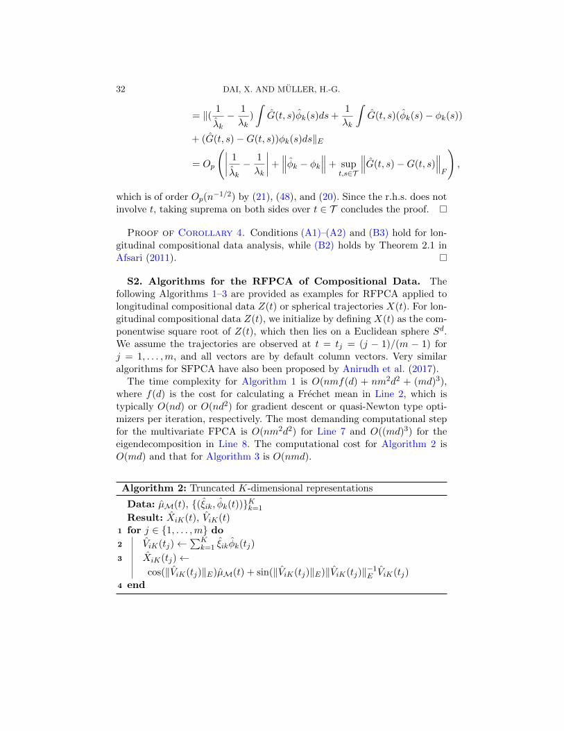
S2. Algorithms for the RFPCA of Compositional Data. Thefollowing Algorithms 1–3 are provided as examples for RFPCA applied tolongitudinal compositional data Z(t) or spherical trajectories X(t). For lon-gitudinal compositional data Z(t), we initialize by defining X(t) as the com-ponentwise square root of Z(t), which then lies on a Euclidean sphere Sd.We assume the trajectories are observed at t = tj = (j − 1)/(m − 1) forj = 1, . . . ,m, and all vectors are by default column vectors. Very similaralgorithms for SFPCA have also been proposed by Anirudh et al. (2017).
The time complexity for Algorithm 1 is O(nmf(d) + nm2d2 + (md)3),where f(d) is the cost for calculating a Frechet mean in Line 2, which istypically O(nd) or O(nd2) for gradient descent or quasi-Newton type opti-mizers per iteration, respectively. The most demanding computational stepfor the multivariate FPCA is O(nm2d2) for Line 7 and O((md)3) for theeigendecomposition in Line 8. The computational cost for Algorithm 2 isO(md) and that for Algorithm 3 is O(nmd).
Algorithm 2: Truncated K-dimensional representations
Data: µM(t), (ξik, φk(t))Kk=1
Result: XiK(t), ViK(t)1 for j ∈ 1, . . . ,m do2 ViK(tj)←
∑Kk=1 ξikφk(tj)
3 XiK(tj)←cos(‖ViK(tj)‖E)µM(t) + sin(‖ViK(tj)‖E)‖ViK(tj)‖−1E ViK(tj)
4 end

FUNCTIONAL DATA ON RIEMANNIAN MANIFOLDS 33
Algorithm 1: Spherical functional principal component analysis(SFPCA)
Data: Sd-valued trajectories X1(t), . . . , Xn(t)Result: µM(t), Vi(t), ξik, φk(t), λk, for i = 1, . . . , n and k = 1, . . . ,K// Obtain the intrinsic mean function and tangent vectors
1 for j ∈ 1, . . . ,m do2 µM(tj)← arg minp∈Sd n−1 ∑n
i=1[cos−1(pTXi(tj))]2
3 for i ∈ 1, . . . , n do
4 Vi(tj) = u√uT u
cos−1(µM(tj)TXi(tj)), where
u = Xi(tj)− (µM(tj)TXi(tj))µM(tj)
5 end
6 end// A multivariate FPCA. Vec(A) stacks the columns of A.
7 Vi ← [Vi(t1), . . . , Vi(tm)]T , G← n−1 ∑ni=1 Vec(Vi)Vec(Vi)
T
8 [ω, Ψ]← Eigen(Vi), for eigenvalues ω = [ω1, . . . , ωm]T and eigenvectorsΨ = [ψ1, . . . , ψm]
9 for k ∈ 1, . . . ,K do
10 Write Φk = [φk(t1), . . . , φk(tm)]T , Vec(Φk)← m1/2ψk, λk ← m−1ωk,
ξik ← m−1Vec(Vi)T Vec(Φk)
11 end
S3. Additional simulations. We conducted an additional simulationstudy to investigate the scalability of the RFPCA algorithms to higher di-mensions d, on the unit sphereM = Sd in Rd+1 for d = 5, 10, 15, 20. Table 5shows that the RFPCA scales well for larger dimensions in terms of runningtime, and its relative disadvantage in speed as compared to the L2 FPCAbecomes smaller as d and n get larger.
The samples were generated in the same fashion as in the main text,except for the mean function µM(t) = expp0(2(d − 1)−1/2t, . . . , 2(d −1)−1/2t, 0.3π sin(πt), 0), and eigenfunctions φk(t) = d−1/2Rt[ζk(t/d), . . . , ζk(t/d+
Algorithm 3: Calculate FVEData: Outputs from Algorithm 1
Result: FVEK1 U0 ← n−1 ∑n
i=1
∫T dM
2(Xi(t), µM(t))dt2 for i ∈ 1, . . . , n do
3 Use Algorithm 2 to obtain XiK(t)4 end
5 UK ← n−1 ∑ni=1
∫T dM
2(Xi(t), XiK(t))dt
6 FVEK = (U0 − UK)/U0
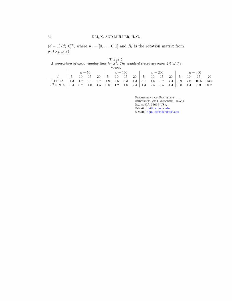
34 DAI, X. AND MULLER, H.-G.
(d − 1)/d), 0]T , where p0 = [0, . . . , 0, 1] and Rt is the rotation matrix fromp0 to µM(t).
Table 5A comparison of mean running time for Sd. The standard errors are below 2% of the
means.
n = 50 n = 100 n = 200 n = 400d 5 10 15 20 5 10 15 20 5 10 15 20 5 10 15 20
RFPCA 1.3 1.7 2.1 2.7 1.9 2.6 3.3 4.3 3.1 4.6 5.7 7.4 5.9 7.8 10.5 13.2L2 FPCA 0.4 0.7 1.0 1.5 0.8 1.2 1.8 2.4 1.4 2.5 3.5 4.4 3.0 4.4 6.3 8.2
Department of StatisticsUniversity of California, DavisDavis, CA 95616 USAE-mail: [email protected]: [email protected]