adaptive functional linear regression via functional ...tcai/paper/adaptive-flr.pdf · adaptive...

Adaptive Functional Linear Regression via Functional

Principal Component Analysis and Block Thresholding∗

T. Tony Cai1, Linjun Zhang1, and Harrison H. Zhou2

University of Pennsylvania and Yale University

Abstract

Theoretical results in the functional linear regression literature have so far fo-

cused on minimax estimation where smoothness parameters are assumed to be

known and the estimators typically depend on these smoothness parameters. In

this paper we consider adaptive estimation in functional linear regression. The goal

is to construct a single data-driven procedure that achieves optimality results si-

multaneously over a collection of parameter spaces. Such an adaptive procedure

automatically adjusts to the smoothness properties of the underlying slope and co-

variance functions. The main technical tools for the construction of the adaptive

procedure are functional principal component analysis and block thresholding. The

estimator of the slope function is shown to adaptively attain the optimal rate of

convergence over a large collection of function spaces.

Keywords: Adaptive estimation; Block thresholding; Eigenfunction; Eigenvalue; Func-

tional data analysis; Functional principal component analysis; Minimax estimation; Rate

of convergence; Slope function; Smoothing; Spectral decomposition.

AMS 2000 Subject Classification: Primary 62J05; secondary 62G20.

∗In Memory of Peter G. Hall.1Department of Statistics, The Wharton School, University of Pennsylvania, Philadelphia, PA 19104.

The research of Tony Cai was supported in part by NSF Grant DMS-1403708 and NIH Grant R01

CA127334.2Department of Statistics, Yale University, New Haven, CT 06511. The research of Harrison Zhou

was supported in part by NSF Grant DMS-1507511.

1

1 Introduction

Due to advances in technology, functional data now commonly arises in many differ-

ent fields of applied sciences including, for example, chemometrics, biomedical studies,

and econometrics. There has been extensive recent research on functional data analysis.

Much progress has been made on developing methodologies for analyzing functional data.

The two monographs by Ramsay and Silverman (2002 and 2005) provide comprehensive

discussions on the methods and applications. See also Ferraty and Vieu (2006).

Among many problems involving functional data, functional linear regression has re-

ceived substantial attention. Consider a functional linear model where one observes a

random sample {(Xi, Yi) : i = 1, ...n} with

Yi = a+

∫ 1

0

Xi(t)b(t)dt+ Zi, (1)

where the response Yi and the intercept a are scalars, the predictor Xi and slope function

b are functions in L2([0, 1]), and the errors Zi are independent and identically distributed

N(0, σ2) variables. The goal is to estimate the slope function b(t) and the intercept a based

on the sample {(Xi, Yi) : i = 1, ...n}. Note that once an estimator b of b is constructed,

the intercept a can be estimated easily by

a = Y −∫ 1

0

X(t)b(t)dt,

where Y and X are the averages of Yi and Xi respectively. We shall thus focus our

discussion in this paper on estimating the slope function b. The slope function is of

significant interest on its own right. For example, knowing where b takes large or small

values provides information about where a future observation x of X will have greatest

leverage on the conditional mean of y given X = x.

The problem of slope-function estimation is intrinsically nonparametric and the con-

vergence rate under the mean integrated squared error (MISE)

R(b, b) = E‖b− b‖22 = E∫ 1

0

(b(t)− b(t))2dt (2)

is typically slower than n−1. Rates of convergence of an estimator b to b have been studied

in, e.g., Ferraty and Vieu (2000); Cuevas et al. (2002); Cardot and Sarda (2006); Li and

Hsing (2007); Hall and Horowitz (2007). In particular, Hall and Horowitz (2007) showed

that the minimax rate of convergence for estimating b under the MISE (2) is determined

by the smoothness of the slope function, and of the covariance function for the distribution

2

of explanatory variables. Cai and Hall (2006) considered a related prediction problem and

Muller and Stadtmuller (2005) studied generalized functional linear models.

The theory on slope function estimation has so far focused on the minimax estimation

where these smoothness parameters are assumed to be known. The estimators typically

depend on the smoothness parameters. Although minimax risk provides a useful uni-

form benchmark for the comparison of estimators, minimax estimators often require full

knowledge of the parameter space which is unknown in practice. A minimax estimator

designed for a specific parameter space typically performs poorly over another parameter

space. This makes adaptation essential for functional linear regression.

In the present paper we consider adaptive estimation of the slope function b. The goal

is to construct a single data-driven procedure that achieves optimality results simultane-

ously over a collection of parameter spaces. Such an adaptive procedure does not require

the knowledge of the parameter space and automatically adjusts to the smoothness prop-

erties of the underlying slope and covariance functions. In Section 2, we construct a

procedure for estimating the slope function b using functional principal component anal-

ysis (PCA) and block thresholding. The estimator is shown to adaptively achieve the

optimal rate of convergence simultaneously over a collection of function classes.

The main technical tools are functional principal component analysis (PCA) and block

thresholding. Functional PCA is a convenient and commonly used technique in functional

data analysis. See, e.g., Ramsay and Silverman (2002 and 2005). Block thresholding was

first developed in nonparametric function estimation. It increases estimation precision

and achieves adaptivity by utilizing information about neighboring coordinates. The idea

of block thresholding can be traced back to Efromovich (1985) in estimating a density

function using the trigonometric basis. It is further developed in wavelet function estima-

tion. See Hall, Kerkyacharian and Picard (1998) for density estimation and Cai (1999) for

nonparametric regression. Cai, Low and Zhao (2009) used weakly geometrically growing

block size for sharp adaptation over ellipsoids in the context of the white noise model. In

this paper we shall follow the ideas in Cai, Low and Zhao (2009) and use weakly geomet-

rically growing block size for adaptive functional linear regression. Our results show that

block thresholding naturally connects shrinkage rules developed in the classical normal

decision theory with functional linear regression.

The proposed block thresholding procedure is easily implementable. A simulation

study is carried out to investigate its numerical performance. In particular, we compare

its finite-sample properties with those of the non-adaptive procedure introduced in Hall

and Horowitz (2007). The results demonstrate the advantage of the proposed procedure.

3

The paper is organized as follows. In Section 2, after basic notations and facts on the

spectral decomposition of the covariance function are reviewed, the block thresholding

procedure for estimating the slope function b is defined in Section 2.2. Section 3 inves-

tigates the theoretical properties of the block thresholding procedure. It is shown that

the estimator enjoys a high degree of adaptivity. Section 4 discusses the numerical per-

formance of the proposed estimator and shows the advantage of the adaptive procedure.

The proofs are given in Section 5.

2 Methodology

Estimating the slope function b in function linear regression involves solving an ill-posed

inverse problem. The main difference with the conventional linear inverse problems is

that the operator is not given in the functional linear regression. A major technical

step in the construction of the slope function estimator is to estimate the eigenvalues

and eigenfunctions of the unknown linear operator and to bound the errors between the

estimates and the estimands. Necessary technical tools for slope function estimation

include functional analysis and statistical smoothing. Specifically, our estimator is based

on the functional principal component analysis and block thresholding techniques. In this

section we will begin with spectral decomposition of the covariance function in terms of

eigenvalues and eigenfunctions. We then introduce in Section 2.2 a blockwise James-Stein

procedure to estimate the slope function b.

2.1 Spectral decomposition

Suppose we observe a random sample {(Xi, Yi) : i = 1, ...n} as in (1). Let (X, Y, Z)

denote a generic (Xi, Yi, Zi). Define the covariance function and the empirical covariance

function respectively as

K(u, v) = cov{X(u), X(v)}

K(u, v) =1

n

n∑i=1

{Xi(u)− X(u)}{Xi(v)− X(v)}

where X = 1n

∑Xi. The covariance function K defines a linear operator which maps a

function f to Kf given by (Kf)(u) =∫K(u, v)f(v)dv. We shall assume that the linear

operator with kernel K is positive definite.

4

Write the spectral decompositions of the covariance functions K and K as

K(u, v) =∞∑j=1

θjφj(u)φj(v), K(u, v) =∞∑j=1

θjφj(u)φj(v), (3)

where

θ1 > θ2 > ... > 0, and θ1 ≥ θ2 ≥ ... ≥ θn+1 = . . . = 0 (4)

are respectively the ordered eigenvalue sequences of the linear operators with kernels K

and K, and {φj} and {φj} are the corresponding orthonormal eigenfunction sequences.

The sequences {φj} and {φj} each forms an orthonormal basis in L2([0, 1]).

The functional linear model (1) can be rewritten as

Yi = µ+

∫[Xi − E(X)] b+ Zi, i = 1, 2, ..., n (5)

where µ = E(Yi) = a + E∫Xb. The Karhunen-Loeve expansion of the random function

Xi − EX is given by

Xi − EX =∞∑j=1

xi,jφj (6)

where the random variable xi,j =∫

(Xi−EX)φj has mean zero and variance Var(xi,j) = θj.

In addition, the random variables xi,j are uncorrelated. Expand the slope function b in

the orthonormal basis {φj} as b =∑∞

j=1 bjφj. Then the model (5) can be written as

Yi = µ+∞∑j=1

xi,jbj + Zi, i = 1, 2, ..., n (7)

and the problem of estimating the slope function b is transformed into the one of estimat-

ing the coefficients {bj} as well as the eigenfunctions {φj}. Note that in (7) µ and xi,j are

unknown, and thus need to be estimated from the data.

The mean µ of Y can be estimated easily by the sample mean µ = Y . To estimate

the xi,j, we expand Xi − X in the orthonormal basis {φj} as

Xi − X =n∑j=1

xi,jφj for i = 1, 2, ..n (8)

where the random variables xi,j =∫

(Xi − X)φj. Note that

n∑i=1

xi,j =n∑i=1

∫(Xi − X)φj =

∫ [ n∑i=1

(Xi − X)

]φj = 0

5

and1

n

n∑i=1

xi,jxi,k =

∫ ∫K(u, v)φj(u)φk(v) = θjδj,k (9)

for all j and k, where δj,k is the Kronecker delta with δj,k = 1 if j = k and 0 otherwise.

Since Y = a+∫ 1

0X(t)b(t)dt+ Z, we have

Yi − Y =

∫ [Xi − X

]b+ Zi − Z, i = 1, 2, ..., n.

Hence

Yi − Y =n∑j=1

xi,j bj + Zi − Z, i = 1, 2, ..., n (10)

where bj =∫bφj, and consequently b =

∑∞j=1 bjφj. Since the slope function b is unknown,

the coefficients bj are also unknown and need to be estimated. A typical principal com-

ponents regression approach is to replace “n” in equation (10) by a constant m < n and

estimate bj by ordinary least squares.

Since the “predictors” (xi,j)1≤j≤n in equation (10) are orthogonal to each other and∑ni=1 x

2i,j = θjn from equation (9), for θj 6= 0 we may estimate bj (or bj) by

bj = θ−1j n−1n∑i=1

(Yi − Y )xi,j = θ−1j n−1n∑i=1

(Yi − Y )

∫ [Xi (u)− X (u)

]φj (u) (11)

= θ−1j

∫g(u)φj (u) = θ−1j gj

where

g(u) = n−1n∑i=1

(Yi − Y )[Xi(u)− X(u)

]and gj =

∫gφj. (12)

It is expected that g is approximately

g(u) = E [(Y − µ) (X(u)− E(X (u))] =

∫ ∫K (u, v) b (v) dv.

Write g =∑∞

j=1 gjφj. It is easy to check that bj = θ−1j gj. So the estimator bj = θ−1j gj

in equation (11) can be regarded as an empirical version of the true coefficient bj. We

shall construct an adaptive estimator of bj based on the empirical coefficients bj by using

a block thresholding technique.

2.2 A Block Thresholding Procedure

Block thresholding techniques have been well developed in nonparametric function esti-

mation literature. See, e.g., Efromovich (1985), Hall, Kerkyacharian and Picard (1998)

6

and Cai (1999). In this paper we shall use a block thresholding method with weakly

geometrically growing block size for adaptive functional linear regression. This method

was used in Cai, Low and Zhao (2009) for sharp adaptive estimation over ellipsoids in the

classical white noise model.

The block thresholding procedures work especially well with homoscedastic Gaussian

data. However, in the current setting the empirical coefficients bj are heteroscedastic

with growing variances. We will see in Lemma 3 in Section 5 that the variance of bj

is approximately σ2θ−1j n−1, getting large as j increases. We shall thus rescale the bj to

stabilize the variances.

With the notation introduced above the block thresholding procedure can then be

described in detail as follows. Let

m∗ = arg min{m : θm/θ1 ≤ n−1/3

}. (13)

It will be shown in Section 5 that there is no need ever to go beyond the m∗-th term

under certain regularity conditions. We define

gj =

{gj j < m∗

0 otherwise

and set

dj = θ− 1

2j gj and dj = θ

− 12

j gj. (14)

Lemma 4 in Section 5 shows that the variance Var(dj) = σ2

n(1+o(1)) and so dj are nearly

homoscedastic. We shall apply a blockwise James-Stein procedure to dj to construct an

estimator dj of dj and then estimate the bj by bj = θ− 1

2j dj.

The block thresholding procedure for estimating the slope function b has three steps.

1. Divide the indices {1, 2, ..., m∗} into nonoverlapping blocks B1, B2, ..., BN with

Card(Bi) =⌊(1 + 1/ log n)i+1

⌋.

2. Apply a blockwise James-Stein rule to each block. For all j ∈ Bi, set

dj = (1− 2Liσ2

nS2i

)+ · dj, (15)

where S2i =

∑j∈Bi d

2j and Li = Card(Bi).

3. Set bj = θ− 1

2j dj. The estimator of b is then given by

b(u) =m∗∑j=1

bjφj(u) =m∗∑j=1

ρj bjφj(u) (16)

7

where ρj = (1− 2Ljσ2

nS2i

)+ for all j ∈ Bi is the shrinkage factor.

The block thresholding procedure given above is purely data-driven and is easy to

implement. In particular it does not require the knowledge of the rate of decay of the

eigenvalues θj or the coefficients bj of the slope function b. In contrast, the minimax rate

optimal estimator given in Hall and Horowitz (2007) critically depends on the rates of

decay of θj and bj.

Remark 1 We have used the blockwise James-Stein procedure in (15) because of its

simplicity. In addition to the James-Stein rule, other shrinkage rules such as the blockwise

hard thresholding rule

dj = dj · I(S2i ≥ λLiσ

2/n)

can be used as well.

Remark 2 In the procedure we assume σ is known, since it can be estimated easily. In

equation (10), we may apply principal components regression by replacing “n” in equation

(10) with a constant m = log2 n. Let bj be the ordinary least squares estimate of bj. It can

be shown easily that∑m

j=1 bjφj is a consistent estimate of b. Then we obtain a consistent

estimate of σ2 with

σ2 =1

n

n∑i=1

(Yi − Y −

m∑j=1

xi,jbj

)2

.

3 Theoretical Properties

We now turn to the asymptotic properties of the block thresholding procedure for the

functional linear regression under the mean integrated squared error (2). The theoret-

ical results show that the block thresholding estimator given in (16) adaptively attains

the exact minimax rate of convergence simultaneously over a large collection of function

spaces.

In this section we shall begin by considering adaptivity of the block thresholding

estimator over the following function spaces which have been considered by Cai and Hall

(2006) and Hall and Horowitz (2007) in the contexts of prediction and slope function

estimation. These function classes arise naturally in functional linear regression based on

functional principal component analysis. For more details, see Cai and Hall (2006) and

Hall and Horowitz (2007). See also Hall and Hosseini-Nasab (2006).

8

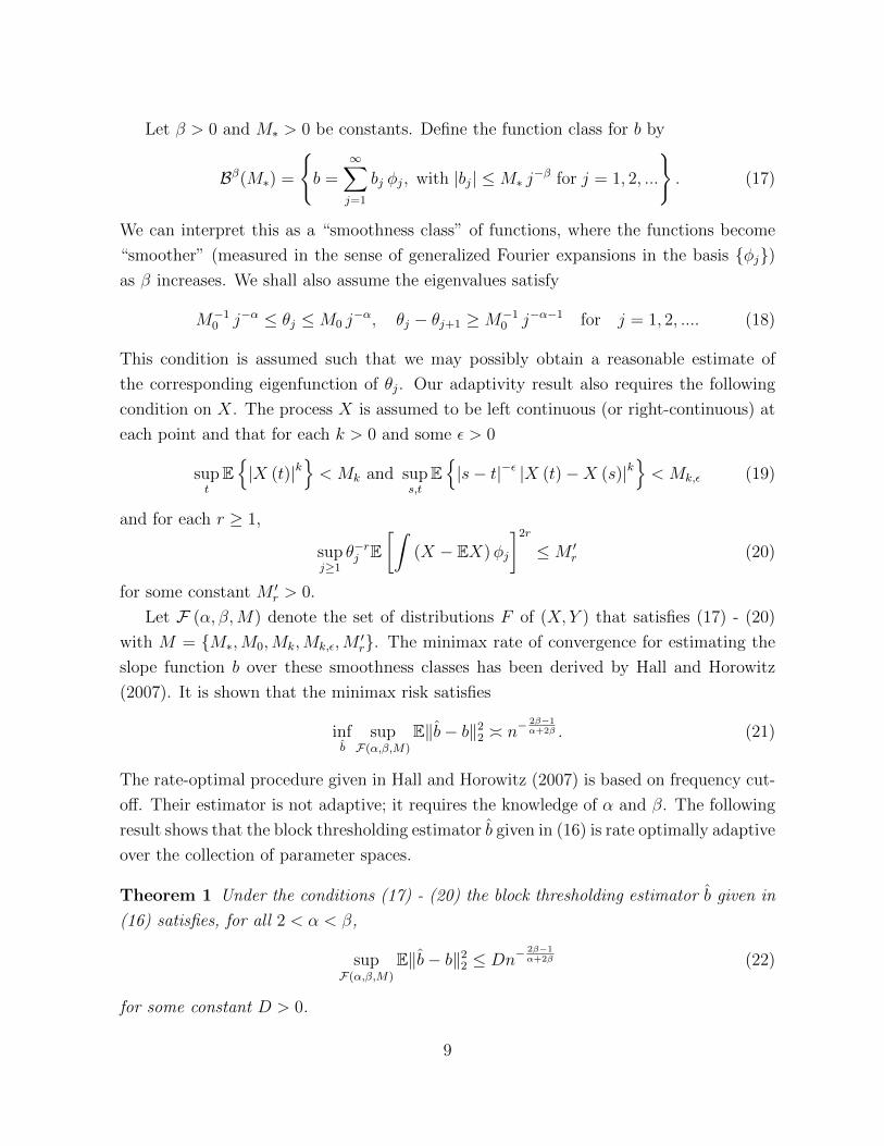
Let β > 0 and M∗ > 0 be constants. Define the function class for b by

Bβ(M∗) =

{b =

∞∑j=1

bj φj, with |bj| ≤M∗ j−β for j = 1, 2, ...

}. (17)

We can interpret this as a “smoothness class” of functions, where the functions become

“smoother” (measured in the sense of generalized Fourier expansions in the basis {φj})as β increases. We shall also assume the eigenvalues satisfy

M−10 j−α ≤ θj ≤M0 j

−α, θj − θj+1 ≥M−10 j−α−1 for j = 1, 2, .... (18)

This condition is assumed such that we may possibly obtain a reasonable estimate of

the corresponding eigenfunction of θj. Our adaptivity result also requires the following

condition on X. The process X is assumed to be left continuous (or right-continuous) at

each point and that for each k > 0 and some ε > 0

supt

E{|X (t)|k

}< Mk and sup

s,tE{|s− t|−ε |X (t)−X (s)|k

}< Mk,ε (19)

and for each r ≥ 1,

supj≥1

θ−rj E[∫

(X − EX)φj

]2r≤M ′

r (20)

for some constant M ′r > 0.

Let F (α, β,M) denote the set of distributions F of (X, Y ) that satisfies (17) - (20)

with M = {M∗,M0,Mk,Mk,ε,M′r}. The minimax rate of convergence for estimating the

slope function b over these smoothness classes has been derived by Hall and Horowitz

(2007). It is shown that the minimax risk satisfies

infb

supF(α,β,M)

E‖b− b‖22 � n−2β−1α+2β . (21)

The rate-optimal procedure given in Hall and Horowitz (2007) is based on frequency cut-

off. Their estimator is not adaptive; it requires the knowledge of α and β. The following

result shows that the block thresholding estimator b given in (16) is rate optimally adaptive

over the collection of parameter spaces.

Theorem 1 Under the conditions (17) - (20) the block thresholding estimator b given in

(16) satisfies, for all 2 < α < β,

supF(α,β,M)

E‖b− b‖22 ≤ Dn−2β−1α+2β (22)

for some constant D > 0.

9

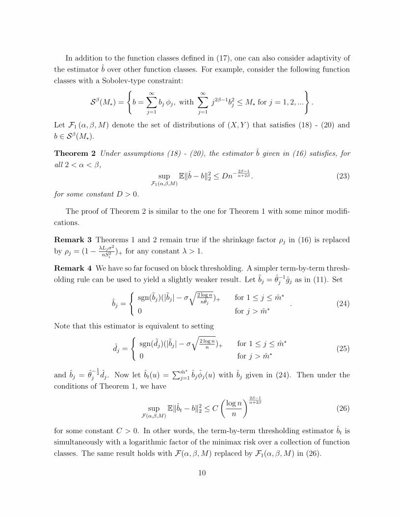
In addition to the function classes defined in (17), one can also consider adaptivity of

the estimator b over other function classes. For example, consider the following function

classes with a Sobolev-type constraint:

Sβ(M∗) =

{b =

∞∑j=1

bj φj, with∞∑j=1

j2β−1b2j ≤M∗ for j = 1, 2, ...

}.

Let F1 (α, β,M) denote the set of distributions of (X, Y ) that satisfies (18) - (20) and

b ∈ Sβ(M∗).

Theorem 2 Under assumptions (18) - (20), the estimator b given in (16) satisfies, for

all 2 < α < β,

supF1(α,β,M)

E‖b− b‖22 ≤ Dn−2β−1α+2β . (23)

for some constant D > 0.

The proof of Theorem 2 is similar to the one for Theorem 1 with some minor modifi-

cations.

Remark 3 Theorems 1 and 2 remain true if the shrinkage factor ρj in (16) is replaced

by ρj = (1− λLjσ2

nS2i

)+ for any constant λ > 1.

Remark 4 We have so far focused on block thresholding. A simpler term-by-term thresh-

olding rule can be used to yield a slightly weaker result. Let bj = θ−1j gj as in (11). Set

bj =

{sgn(bj)(|bj| − σ

√2 logn

nθj)+ for 1 ≤ j ≤ m∗

0 for j > m∗. (24)

Note that this estimator is equivalent to setting

dj =

{sgn(dj)(|bj| − σ

√2 lognn

)+ for 1 ≤ j ≤ m∗

0 for j > m∗(25)

and bj = θ− 1

2j dj. Now let bt(u) =

∑m∗

j=1 bjφj(u) with bj given in (24). Then under the

conditions of Theorem 1, we have

supF(α,β,M)

E‖bt − b‖22 ≤ C

(log n

n

) 2β−1α+2β

(26)

for some constant C > 0. In other words, the term-by-term thresholding estimator bt is

simultaneously with a logarithmic factor of the minimax risk over a collection of function

classes. The same result holds with F(α, β,M) replaced by F1(α, β,M) in (26).

10

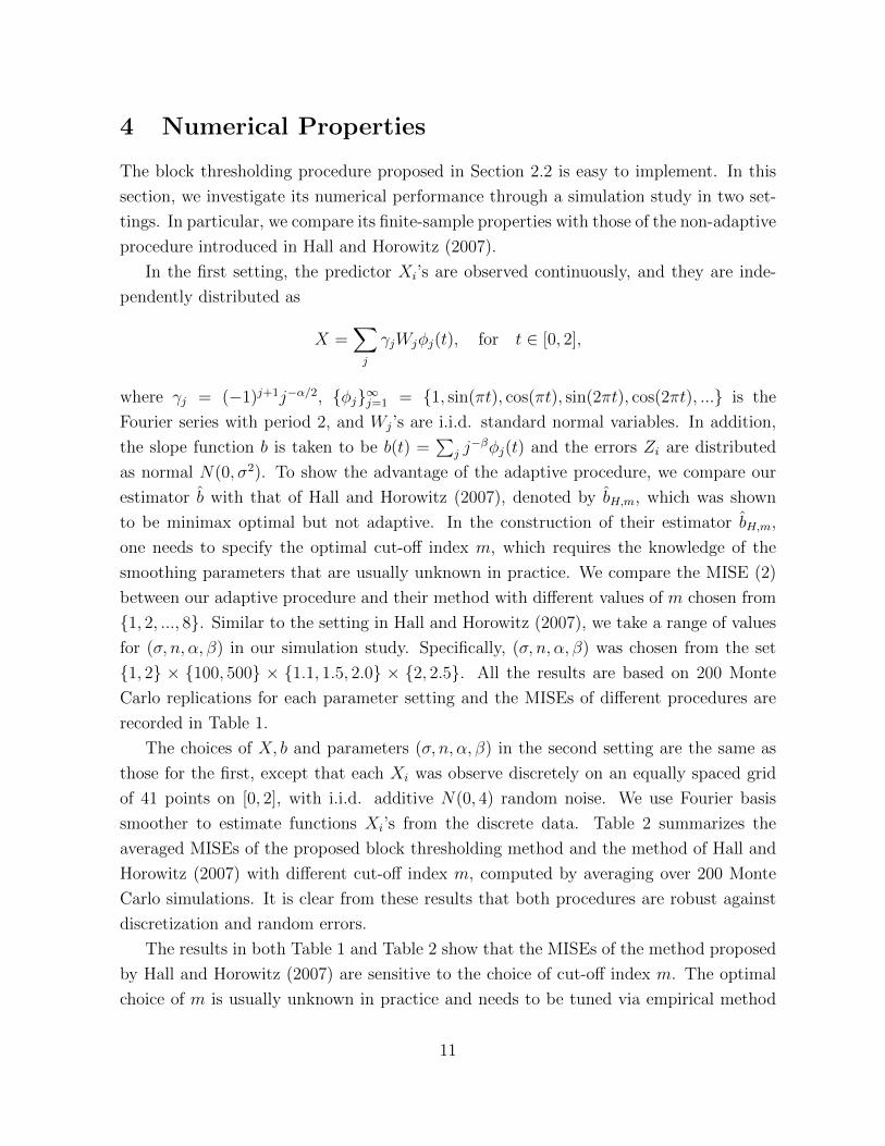
4 Numerical Properties

The block thresholding procedure proposed in Section 2.2 is easy to implement. In this

section, we investigate its numerical performance through a simulation study in two set-

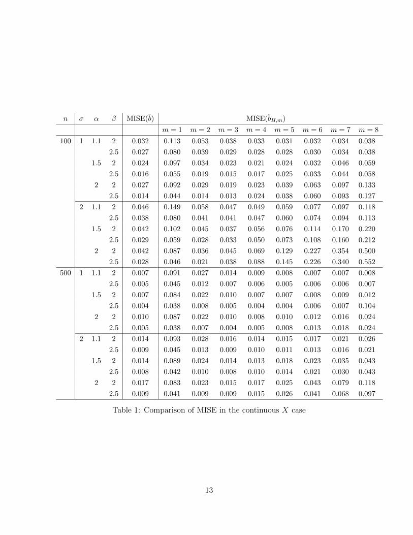
tings. In particular, we compare its finite-sample properties with those of the non-adaptive

procedure introduced in Hall and Horowitz (2007).

In the first setting, the predictor Xi’s are observed continuously, and they are inde-

pendently distributed as

X =∑j

γjWjφj(t), for t ∈ [0, 2],

where γj = (−1)j+1j−α/2, {φj}∞j=1 = {1, sin(πt), cos(πt), sin(2πt), cos(2πt), ...} is the

Fourier series with period 2, and Wj’s are i.i.d. standard normal variables. In addition,

the slope function b is taken to be b(t) =∑

j j−βφj(t) and the errors Zi are distributed

as normal N(0, σ2). To show the advantage of the adaptive procedure, we compare our

estimator b with that of Hall and Horowitz (2007), denoted by bH,m, which was shown

to be minimax optimal but not adaptive. In the construction of their estimator bH,m,

one needs to specify the optimal cut-off index m, which requires the knowledge of the

smoothing parameters that are usually unknown in practice. We compare the MISE (2)

between our adaptive procedure and their method with different values of m chosen from

{1, 2, ..., 8}. Similar to the setting in Hall and Horowitz (2007), we take a range of values

for (σ, n, α, β) in our simulation study. Specifically, (σ, n, α, β) was chosen from the set

{1, 2} × {100, 500} × {1.1, 1.5, 2.0} × {2, 2.5}. All the results are based on 200 Monte

Carlo replications for each parameter setting and the MISEs of different procedures are

recorded in Table 1.

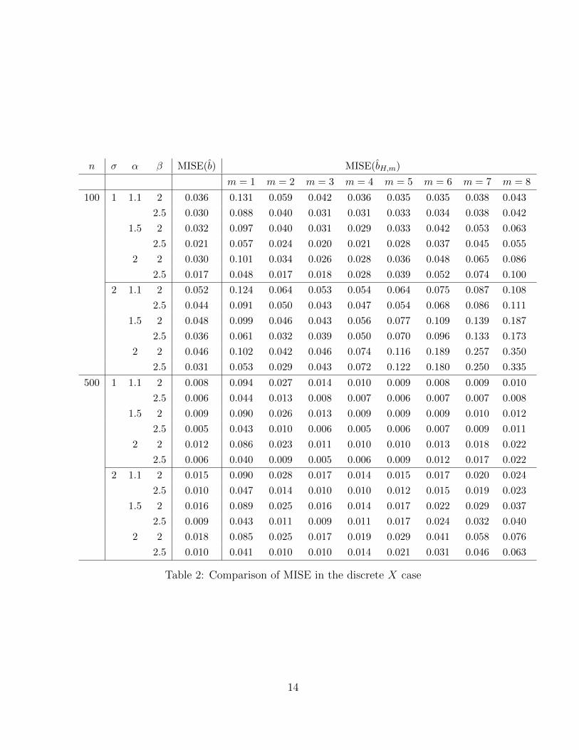
The choices of X, b and parameters (σ, n, α, β) in the second setting are the same as

those for the first, except that each Xi was observe discretely on an equally spaced grid

of 41 points on [0, 2], with i.i.d. additive N(0, 4) random noise. We use Fourier basis

smoother to estimate functions Xi’s from the discrete data. Table 2 summarizes the

averaged MISEs of the proposed block thresholding method and the method of Hall and

Horowitz (2007) with different cut-off index m, computed by averaging over 200 Monte

Carlo simulations. It is clear from these results that both procedures are robust against

discretization and random errors.

The results in both Table 1 and Table 2 show that the MISEs of the method proposed

by Hall and Horowitz (2007) are sensitive to the choice of cut-off index m. The optimal

choice of m is usually unknown in practice and needs to be tuned via empirical method

11

such as cross validation. In contrast, our proposed method is purely data-driven and

adaptive to different degrees of smoothness. Both tables demonstrate the advantage of

the proposed adaptive procedure. The performance of the proposed adaptive method is

as good as, if not better than, the method of Hall and Horowitz (2007) with the optimally

chosen m.

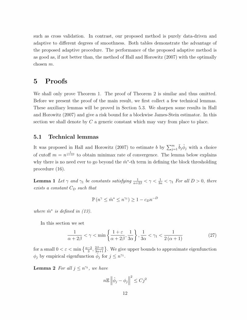
5 Proofs

We shall only prove Theorem 1. The proof of Theorem 2 is similar and thus omitted.

Before we present the proof of the main result, we first collect a few technical lemmas.

These auxiliary lemmas will be proved in Section 5.3. We sharpen some results in Hall

and Horowitz (2007) and give a risk bound for a blockwise James-Stein estimator. In this

section we shall denote by C a generic constant which may vary from place to place.

5.1 Technical lemmas

It was proposed in Hall and Horowitz (2007) to estimate b by∑m

j=1 bjφj with a choice

of cutoff m = n1

α+2β to obtain minimax rate of convergence. The lemma below explains

why there is no need ever to go beyond the m∗-th term in defining the block thresholding

procedure (16).

Lemma 1 Let γ and γ1 be constants satisfying 1α+2β

< γ < 13α< γ1 For all D > 0, there

exists a constant CD such that

P (nγ ≤ m∗ ≤ nγ1) ≥ 1− cDn−D

where m∗ is defined in (13).

In this section we set

1

α + 2β< γ < min

{1 + ε

α + 2β,

1

3α

},

1

3α< γ1 <

1

2 (α + 1)(27)

for a small 0 < ε < min{α−23, 2β−α3α+1

}. We give upper bounds to approximate eigenfunction

φj by empirical eigenfunction φj for j ≤ nγ1 .

Lemma 2 For all j ≤ nγ1, we have

nE∥∥∥φj − φj∥∥∥2 ≤ Cj2

12

n σ α β MISE(b) MISE(bH,m)

m = 1 m = 2 m = 3 m = 4 m = 5 m = 6 m = 7 m = 8

100 1 1.1 2 0.032 0.113 0.053 0.038 0.033 0.031 0.032 0.034 0.038

2.5 0.027 0.080 0.039 0.029 0.028 0.028 0.030 0.034 0.038

1.5 2 0.024 0.097 0.034 0.023 0.021 0.024 0.032 0.046 0.059

2.5 0.016 0.055 0.019 0.015 0.017 0.025 0.033 0.044 0.058

2 2 0.027 0.092 0.029 0.019 0.023 0.039 0.063 0.097 0.133

2.5 0.014 0.044 0.014 0.013 0.024 0.038 0.060 0.093 0.127

2 1.1 2 0.046 0.149 0.058 0.047 0.049 0.059 0.077 0.097 0.118

2.5 0.038 0.080 0.041 0.041 0.047 0.060 0.074 0.094 0.113

1.5 2 0.042 0.102 0.045 0.037 0.056 0.076 0.114 0.170 0.220

2.5 0.029 0.059 0.028 0.033 0.050 0.073 0.108 0.160 0.212

2 2 0.042 0.087 0.036 0.045 0.069 0.129 0.227 0.354 0.500

2.5 0.028 0.046 0.021 0.038 0.088 0.145 0.226 0.340 0.552

500 1 1.1 2 0.007 0.091 0.027 0.014 0.009 0.008 0.007 0.007 0.008

2.5 0.005 0.045 0.012 0.007 0.006 0.005 0.006 0.006 0.007

1.5 2 0.007 0.084 0.022 0.010 0.007 0.007 0.008 0.009 0.012

2.5 0.004 0.038 0.008 0.005 0.004 0.004 0.006 0.007 0.104

2 2 0.010 0.087 0.022 0.010 0.008 0.010 0.012 0.016 0.024

2.5 0.005 0.038 0.007 0.004 0.005 0.008 0.013 0.018 0.024

2 1.1 2 0.014 0.093 0.028 0.016 0.014 0.015 0.017 0.021 0.026

2.5 0.009 0.045 0.013 0.009 0.010 0.011 0.013 0.016 0.021

1.5 2 0.014 0.089 0.024 0.014 0.013 0.018 0.023 0.035 0.043

2.5 0.008 0.042 0.010 0.008 0.010 0.014 0.021 0.030 0.043

2 2 0.017 0.083 0.023 0.015 0.017 0.025 0.043 0.079 0.118

2.5 0.009 0.041 0.009 0.009 0.015 0.026 0.041 0.068 0.097

Table 1: Comparison of MISE in the continuous X case

13

n σ α β MISE(b) MISE(bH,m)

m = 1 m = 2 m = 3 m = 4 m = 5 m = 6 m = 7 m = 8

100 1 1.1 2 0.036 0.131 0.059 0.042 0.036 0.035 0.035 0.038 0.043

2.5 0.030 0.088 0.040 0.031 0.031 0.033 0.034 0.038 0.042

1.5 2 0.032 0.097 0.040 0.031 0.029 0.033 0.042 0.053 0.063

2.5 0.021 0.057 0.024 0.020 0.021 0.028 0.037 0.045 0.055

2 2 0.030 0.101 0.034 0.026 0.028 0.036 0.048 0.065 0.086

2.5 0.017 0.048 0.017 0.018 0.028 0.039 0.052 0.074 0.100

2 1.1 2 0.052 0.124 0.064 0.053 0.054 0.064 0.075 0.087 0.108

2.5 0.044 0.091 0.050 0.043 0.047 0.054 0.068 0.086 0.111

1.5 2 0.048 0.099 0.046 0.043 0.056 0.077 0.109 0.139 0.187

2.5 0.036 0.061 0.032 0.039 0.050 0.070 0.096 0.133 0.173

2 2 0.046 0.102 0.042 0.046 0.074 0.116 0.189 0.257 0.350

2.5 0.031 0.053 0.029 0.043 0.072 0.122 0.180 0.250 0.335

500 1 1.1 2 0.008 0.094 0.027 0.014 0.010 0.009 0.008 0.009 0.010

2.5 0.006 0.044 0.013 0.008 0.007 0.006 0.007 0.007 0.008

1.5 2 0.009 0.090 0.026 0.013 0.009 0.009 0.009 0.010 0.012

2.5 0.005 0.043 0.010 0.006 0.005 0.006 0.007 0.009 0.011

2 2 0.012 0.086 0.023 0.011 0.010 0.010 0.013 0.018 0.022

2.5 0.006 0.040 0.009 0.005 0.006 0.009 0.012 0.017 0.022

2 1.1 2 0.015 0.090 0.028 0.017 0.014 0.015 0.017 0.020 0.024

2.5 0.010 0.047 0.014 0.010 0.010 0.012 0.015 0.019 0.023

1.5 2 0.016 0.089 0.025 0.016 0.014 0.017 0.022 0.029 0.037

2.5 0.009 0.043 0.011 0.009 0.011 0.017 0.024 0.032 0.040

2 2 0.018 0.085 0.025 0.017 0.019 0.029 0.041 0.058 0.076

2.5 0.010 0.041 0.010 0.010 0.014 0.021 0.031 0.046 0.063

Table 2: Comparison of MISE in the discrete X case

14

and for any given 0 < δ < 1 and for all D > 0 there exists a constant CD > 0 such that

P{n1−δ

∥∥∥φj − φj∥∥∥2 ≥ Cj2}≤ CDn

−D.

Lemma 3 gives a variance bound for bj, which helps us show that the variance of dj

is approximately σ2

n. This result is crucial for proposing a practical block thresholding

procedure.

Lemma 3 For j ≤ nγ1 with γ1 <1

2(α+1),

E(bj − bj

)2 ≤ Cj2/n.

In particular, this implies Var(bj) ≤ Cj2/n and Var(bj) = σ2θ−1j n−1 (1 + o (1)).

The following lemma gives bounds for the variance and mean squared error of dj.

Lemma 4 For j ≤ nγ1 with γ1 <1

2(α+1),

Var(dj) =σ2

n(1 + o (1)) and E

(dj − θ

12j bj

)2≤ Cn−1j2−α.

The following two lemmas will be used to analyze the factor ρj in equation (16).

Lemma 5 Let nγ ≤ m1 ≤ m2 ≤ nγ1 and m2 − m1 ≥ nδ for some δ > 0. Define

S2 =∑m2

j=m1d2j . For any given ε > 0 and all D > 0 there exists a constant CD > 0 such

that

P(S2 > (1 + ε) (m2 −m1)σ2

n) ≤ CDn

−D.

Lemma 6 Let dj = d′j + εj where d′j = E(dj). Let ε > 0 be a fixed constant. If the block

size Li = Card(Bi) ≥ nδ for some δ > 0, then for any D > 0, there exists a constant

CD > 0 such that

P(∑j∈Bi

ε2j > (1 + ε)Liσ2

n) ≤ CDn

−D. (28)

And for all blocks Bi,

E∑j∈Bi

ε2j ≤ CLiσ2

n. (29)

Conventional oracle inequalities were derived for Gaussian errors. In the current set-

ting the errors are non-Gaussian. The following lemma gives an oracle inequality for a

block thresholding estimator in the case of general error distributions. See Brown, Cai,

Zhang, Zhao and Zhou (2010) for a proof.

15

Lemma 7 Suppose yi = θi + εi, i = 1, ..., L, where θi are constants and Zi are random

variables. Let S2 =∑L

i=1 y2i and let

θi = (1− λL

S2)+yi.

Then

E‖θ − θ‖22 ≤ min{‖θ‖22, 4λL}+ 4E‖ε‖22I(‖ε‖22 > λL). (30)

5.2 Proof of Theorem 1

We shall prove Theorem 1 for a general block thresholding estimator with the shrinkage

factor ρj = (1− λLjσ2

nS2i

)+ for a constant λ > 1.

Let γ and γ1 be constants satisfying

1

α + 2β< γ < min

{1 + ε

α + 2β,

1

3α

}≤ 1

3α< γ1 <

1

2 (α + 1)

for a small ε > 0. Let m∗ = nγ and write b as

b(u) =m∗∑j=1

ρj bjφj(u) +n∑

j=m∗+1

ρj bjφj(u). (31)

We shall show that E‖b− b‖22 ≤ Cn−2β−1α+2β . Note that

E‖b− b‖22 = E‖m∗∑j=1

bjφj(u) +n∑

j=m∗+1

bjφj(u)−m∗∑j=1

bjφj(u)−∞∑

j=m∗+1

bjφj(u)‖22

≤ 3E‖m∗∑j=1


bjφj(u)‖22 + 3n∑

j=m∗+1

E(b2j) + 3∞∑

j=m∗+1

b2j . (32)

The last term (32) is bounded by Cn−γ(2β−1) = o(n−(2β−1)/(α+2β)

)since γ > 1

α+2β. We

first show that the second term (32) is small as well. Let m∗ = nγ1 and let i∗ and i∗ be

the corresponding block indices of the (m∗ + 1)-st and m∗-th term respectively. (That is,

bm∗+1 is in the i∗-th block and bm∗ is in the i∗-th block.) Then it follows from Lemmas 1

and 5 that

n∑j=m∗+1

E(b2j) =

(m∗∑

j=m∗+1

+n∑

j=m∗+1

)E(ρ2j b

2j)

≤m∗∑

j=m∗+1

(Eρ4j)12 (Eb4j)

12 +

n∑j=m∗+1

(Eb4j)12P

12 (m∗ ≥ nγ1 + 1)

16

≤i∗∑i=i∗

[P(S2

i > λLσ2/n)]1/2 ∑

j∈Bi

(Eb4j)12 +

n∑j=m∗+1

(Eb4j)12 [P (m∗ ≥ nγ1 + 1)]1/2

= o(n−

2β−1α+2β

).

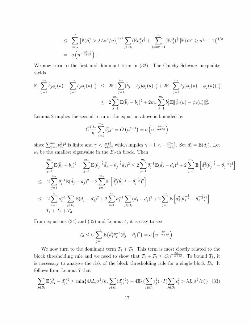
We now turn to the first and dominant term in (32). The Cauchy-Schwarz inequality

yields

E‖m∗∑j=1


bjφj(u)‖22 ≤ 2E‖m∗∑j=1

(bj − bj)φj(u)‖22 + 2E‖m∗∑j=1

bj(φj(u)− φj(u))‖22

≤ 2m∗∑j=1

E(bj − bj)2 + 2m∗

m∗∑j=1

b2jE‖φj(u)− φj(u)‖22.

Lemma 2 implies the second term in the equation above is bounded by

Cm∗n

m∗∑j=1

b2jj2 = O

(nγ−1

)= o

(n−

2β−1α+2β

)since

∑m∗j=1 b

2jj

2 is finite and γ < α+1α+2β

which implies γ − 1 < − 2β−1α+2β

. Set d′j = E(dj). Let

κi be the smallest eigenvalue in the Bi-th block. Then

m∗∑j=1

E(bj − bj)2 =m∗∑j=1

E(θ− 1

2j dj − θ

− 12

j dj)2 ≤ 2

m∗∑j=1

θ−1j E(dj − dj)2 + 2m∗∑j=1

E[d2j(θ

− 12

j − θ− 1

2j )2

]≤ 2

m∗∑j=1

θ−1j E(dj − dj)2 + 2m∗∑j=1

E[d2j(θ

− 12

j − θ− 1

2j )2

]≤ 2

i∗∑i=1

κ−1i∑j∈Bi

E(dj − d′j)2 + 2i∗∑i=1

κ−1i∑j∈Bi

(d′j − dj)2 + 2m∗∑j=1

E[d2j(θ

− 12

j − θ− 1

2j )2

]≡ T1 + T2 + T3.

From equations (34) and (35) and Lemma 4, it is easy to see

T3 ≤ C

m∗∑j=1

E{d2jθ−3j (θj − θj)2} = o(n−

2β−1α+2β

).

We now turn to the dominant term T1 + T2. This term is most closely related to the

block thresholding rule and we need to show that T1 + T2 ≤ Cn−2β−1α+2β . To bound T1, it

is necessary to analyze the risk of the block thresholding rule for a single block Bi. It

follows from Lemma 7 that∑j∈Bi

E(dj − d′j)2 ≤ min{4λLiσ2/n,∑j∈Bi

(d′j)2}+ 4E{(

∑j∈Bi

ε2j) · I(∑j∈Bi

ε2j > λLiσ2/n)} (33)

17

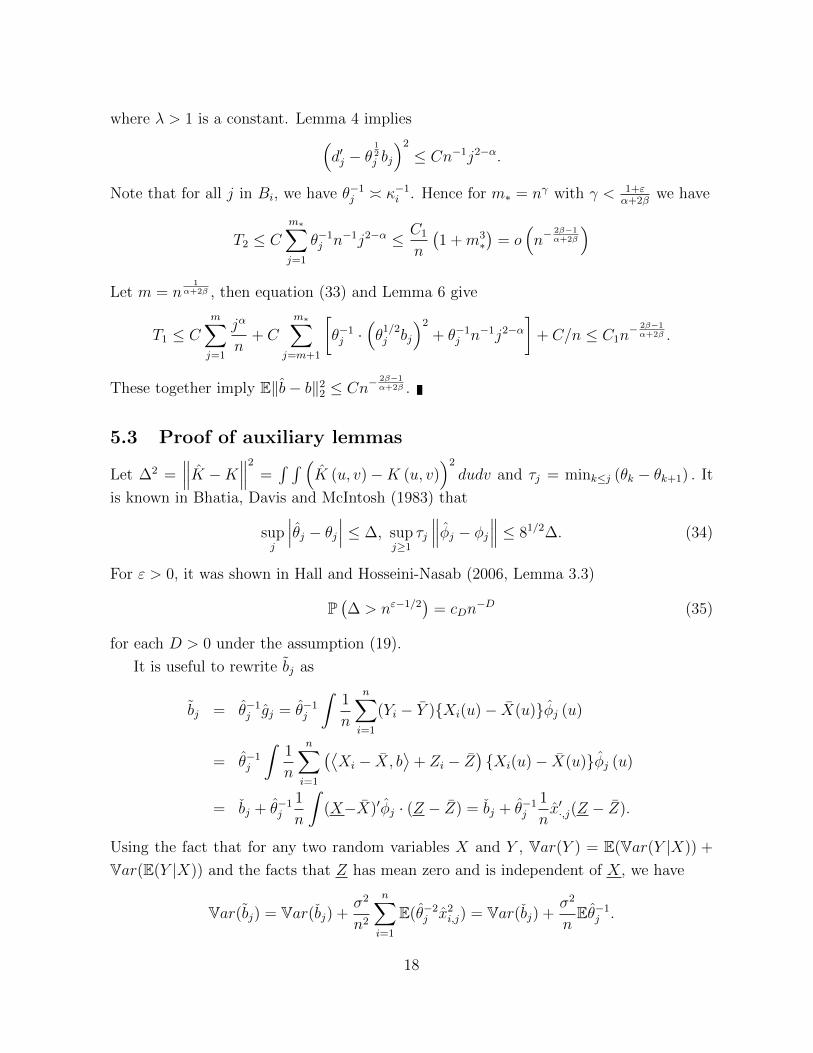
where λ > 1 is a constant. Lemma 4 implies(d′j − θ

12j bj

)2≤ Cn−1j2−α.

Note that for all j in Bi, we have θ−1j � κ−1i . Hence for m∗ = nγ with γ < 1+εα+2β

we have

T2 ≤ Cm∗∑j=1

θ−1j n−1j2−α ≤ C1

n

(1 +m3

∗)

= o(n−

2β−1α+2β

)Let m = n

1α+2β , then equation (33) and Lemma 6 give

T1 ≤ C

m∑j=1

jα

n+ C

m∗∑j=m+1

[θ−1j ·

(θ1/2j bj

)2+ θ−1j n−1j2−α

]+ C/n ≤ C1n

− 2β−1α+2β .

These together imply E‖b− b‖22 ≤ Cn−2β−1α+2β .

5.3 Proof of auxiliary lemmas

Let ∆2 =∥∥∥K −K∥∥∥2 =

∫ ∫ (K (u, v)−K (u, v)

)2dudv and τj = mink≤j (θk − θk+1) . It

is known in Bhatia, Davis and McIntosh (1983) that

supj

∣∣∣θj − θj∣∣∣ ≤ ∆, supj≥1

τj

∥∥∥φj − φj∥∥∥ ≤ 81/2∆. (34)

For ε > 0, it was shown in Hall and Hosseini-Nasab (2006, Lemma 3.3)

P(∆ > nε−1/2

)= cDn

−D (35)

for each D > 0 under the assumption (19).

It is useful to rewrite bj as

bj = θ−1j gj = θ−1j

∫1

n

n∑i=1

(Yi − Y ){Xi(u)− X(u)}φj (u)

= θ−1j

∫1

n

n∑i=1

(⟨Xi − X, b

⟩+ Zi − Z

){Xi(u)− X(u)}φj (u)

= bj + θ−1j1

n

∫(X−X)′φj · (Z − Z) = bj + θ−1j

1

nx′·,j(Z − Z).

Using the fact that for any two random variables X and Y , Var(Y ) = E(Var(Y |X)) +

Var(E(Y |X)) and the facts that Z has mean zero and is independent of X, we have

Var(bj) = Var(bj) +σ2

n2

n∑i=1

E(θ−2j x2i,j) = Var(bj) +σ2

nEθ−1j .

18

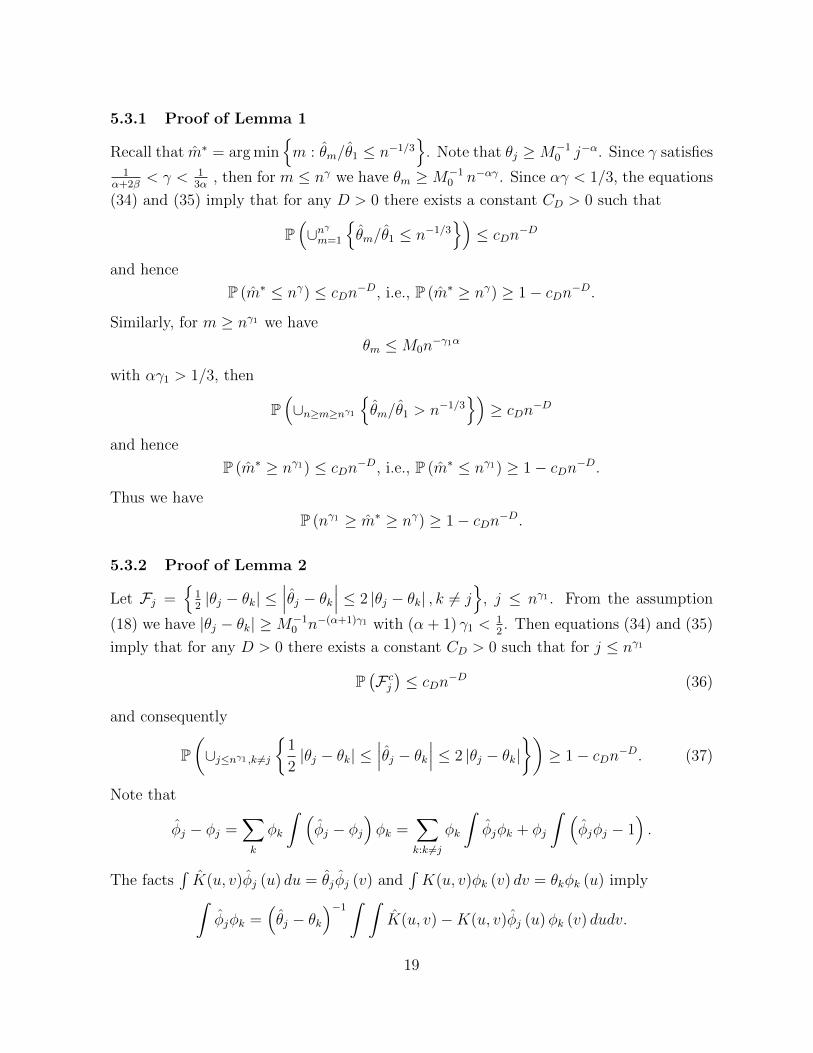
5.3.1 Proof of Lemma 1

Recall that m∗ = arg min{m : θm/θ1 ≤ n−1/3

}. Note that θj ≥M−1

0 j−α. Since γ satisfies1

α+2β< γ < 1

3α, then for m ≤ nγ we have θm ≥M−1

0 n−αγ. Since αγ < 1/3, the equations

(34) and (35) imply that for any D > 0 there exists a constant CD > 0 such that

P(∪nγm=1

{θm/θ1 ≤ n−1/3

})≤ cDn

−D

and hence

P (m∗ ≤ nγ) ≤ cDn−D, i.e., P (m∗ ≥ nγ) ≥ 1− cDn−D.

Similarly, for m ≥ nγ1 we have

θm ≤M0n−γ1α

with αγ1 > 1/3, then

P(∪n≥m≥nγ1

{θm/θ1 > n−1/3

})≥ cDn

−D

and hence

P (m∗ ≥ nγ1) ≤ cDn−D, i.e., P (m∗ ≤ nγ1) ≥ 1− cDn−D.

Thus we have

P (nγ1 ≥ m∗ ≥ nγ) ≥ 1− cDn−D.


Let Fj ={

12|θj − θk| ≤

∣∣∣θj − θk∣∣∣ ≤ 2 |θj − θk| , k 6= j}

, j ≤ nγ1 . From the assumption

(18) we have |θj − θk| ≥M−10 n−(α+1)γ1 with (α + 1) γ1 <

12. Then equations (34) and (35)

imply that for any D > 0 there exists a constant CD > 0 such that for j ≤ nγ1

P(F cj)≤ cDn

−D (36)

and consequently

P(∪j≤nγ1 ,k 6=j

{1

2|θj − θk| ≤

∣∣∣θj − θk∣∣∣ ≤ 2 |θj − θk|})≥ 1− cDn−D. (37)

Note that

φj − φj =∑k

φk

∫ (φj − φj

)φk =

∑k:k 6=j

φk

∫φjφk + φj

∫ (φjφj − 1

).

The facts∫K(u, v)φj (u) du = θjφj (v) and

∫K(u, v)φk (v) dv = θkφk (u) imply∫

φjφk =(θj − θk

)−1 ∫ ∫K(u, v)−K(u, v)φj (u)φk (v) dudv.

19

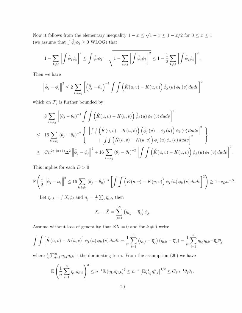
Now it follows from the elementary inequality 1 − x ≤√

1− x ≤ 1 − x/2 for 0 ≤ x ≤ 1

(we assume that∫φjφj ≥ 0 WLOG) that

1−∑k 6=j

[∫φjφk

]2≤∫φjφj =

√√√√1−∑k 6=j

[∫φjφk

]2≤ 1− 1

2

∑k 6=j

[∫φjφk

]2.

Then we have∥∥∥φj − φj∥∥∥2 ≤ 2∑k:k 6=j

[(θj − θk

)−1 ∫ ∫ (K(u, v)−K(u, v)

)φj (u)φk (v) dudv

]2which on Fj is further bounded by

8∑k:k 6=j

[(θj − θk)−1

∫ ∫ (K(u, v)−K(u, v)


]2

≤ 16∑k:k 6=j

(θj − θk)−2[∫ ∫ (

K(u, v)−K(u, v))(

φj (u)− φj (u))φk (v) dudv

]2+[∫ ∫ (

K(u, v)−K(u, v))φj (u)φk (v) dudv

]2

≤ Cn2γ1(α+1)∆2∥∥∥φj − φj∥∥∥2 + 16

∑k:k 6=j

(θj − θk)−2[∫ ∫ (


]2.

This implies for each D > 0

P

(1

2

∥∥∥φj − φj∥∥∥2 ≤ 16∑k:k 6=j

(θj − θk)−2[∫ ∫ (


]2)≥ 1−cDn−D.

Let ηi,j =∫Xiφj and ηj = 1

n

∑i ηi,j, then

Xi − X =∞∑j=1

(ηi,j − ηj

)φj.

Assume without loss of generality that EX = 0 and for k 6= j write∫ ∫ [K(u, v)−K(u, v)

]φj (u)φk (v) dudv =

1

n

n∑i=1

(ηi,j − ηj

)(ηi,k − ηk) =

1

n

n∑i=1

ηi,jηi,k−ηkηj

where 1n

∑ni=1 ηi,jηi,k is the dominating term. From the assumption (20) we have

E

(1

n

n∑i=1

ηi,jηi,k

)2

≤ n−1E (η1,jη1,k)2 ≤ n−1

[Eη41,jη41,k

]1/2 ≤ C1n−1θjθk.

20

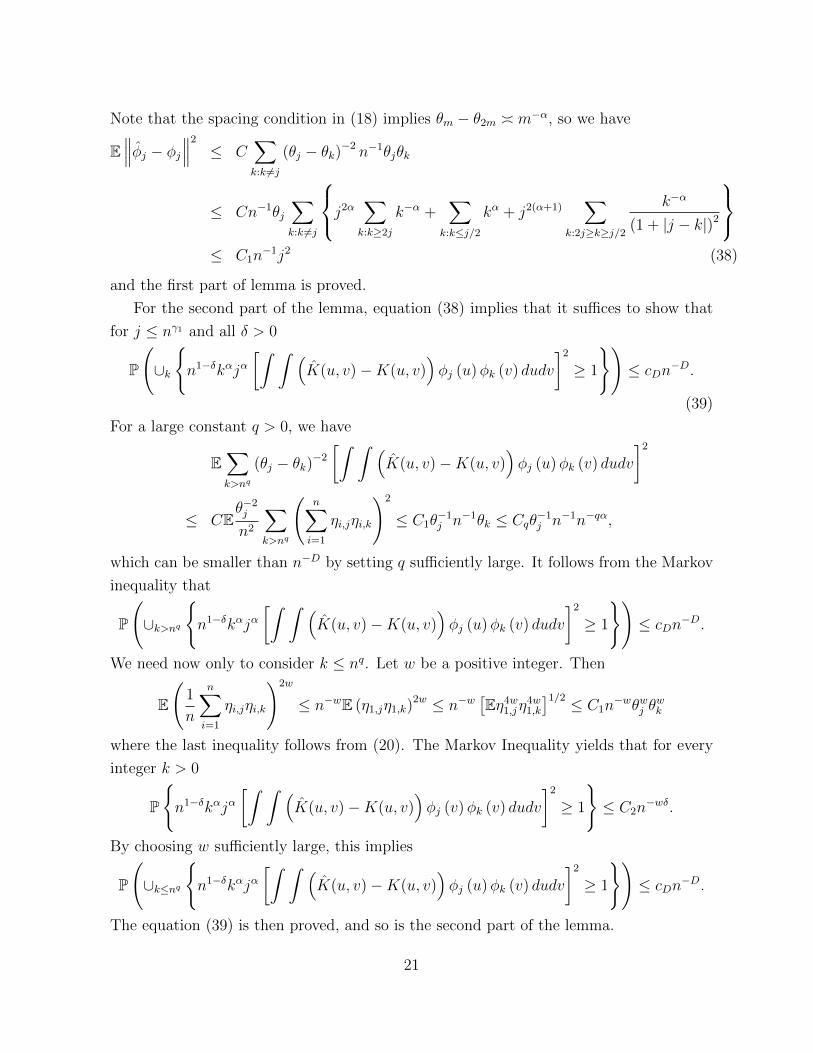
Note that the spacing condition in (18) implies θm − θ2m � m−α, so we have

E∥∥∥φj − φj∥∥∥2 ≤ C

∑k:k 6=j

(θj − θk)−2 n−1θjθk

≤ Cn−1θj∑k:k 6=j

j2α ∑k:k≥2j

k−α +∑

k:k≤j/2

kα + j2(α+1)∑

k:2j≥k≥j/2

k−α

(1 + |j − k|)2

≤ C1n

−1j2 (38)

and the first part of lemma is proved.

For the second part of the lemma, equation (38) implies that it suffices to show that

for j ≤ nγ1 and all δ > 0

P

(∪k

{n1−δkαjα

[∫ ∫ (K(u, v)−K(u, v)


]2≥ 1

})≤ cDn

−D.

(39)

For a large constant q > 0, we have

E∑k>nq

(θj − θk)−2[∫ ∫ (


]2

≤ CEθ−2jn2

∑k>nq

(n∑i=1

ηi,jηi,k

)2

≤ C1θ−1j n−1θk ≤ Cqθ

−1j n−1n−qα,

which can be smaller than n−D by setting q sufficiently large. It follows from the Markov

inequality that

P

(∪k>nq

{n1−δkαjα

[∫ ∫ (K(u, v)−K(u, v)


]2≥ 1

})≤ cDn

−D.

We need now only to consider k ≤ nq. Let w be a positive integer. Then

E

(1

n

n∑i=1

ηi,jηi,k

)2w

≤ n−wE (η1,jη1,k)2w ≤ n−w

[Eη4w1,jη4w1,k

]1/2 ≤ C1n−wθwj θ

wk

where the last inequality follows from (20). The Markov Inequality yields that for every

integer k > 0

P

{n1−δkαjα

[∫ ∫ (K(u, v)−K(u, v)

)φj (v)φk (v) dudv

]2≥ 1

}≤ C2n

−wδ.

By choosing w sufficiently large, this implies

P

(∪k≤nq

{n1−δkαjα

[∫ ∫ (K(u, v)−K(u, v)


]2≥ 1

})≤ cDn

−D.

The equation (39) is then proved, and so is the second part of the lemma.

21

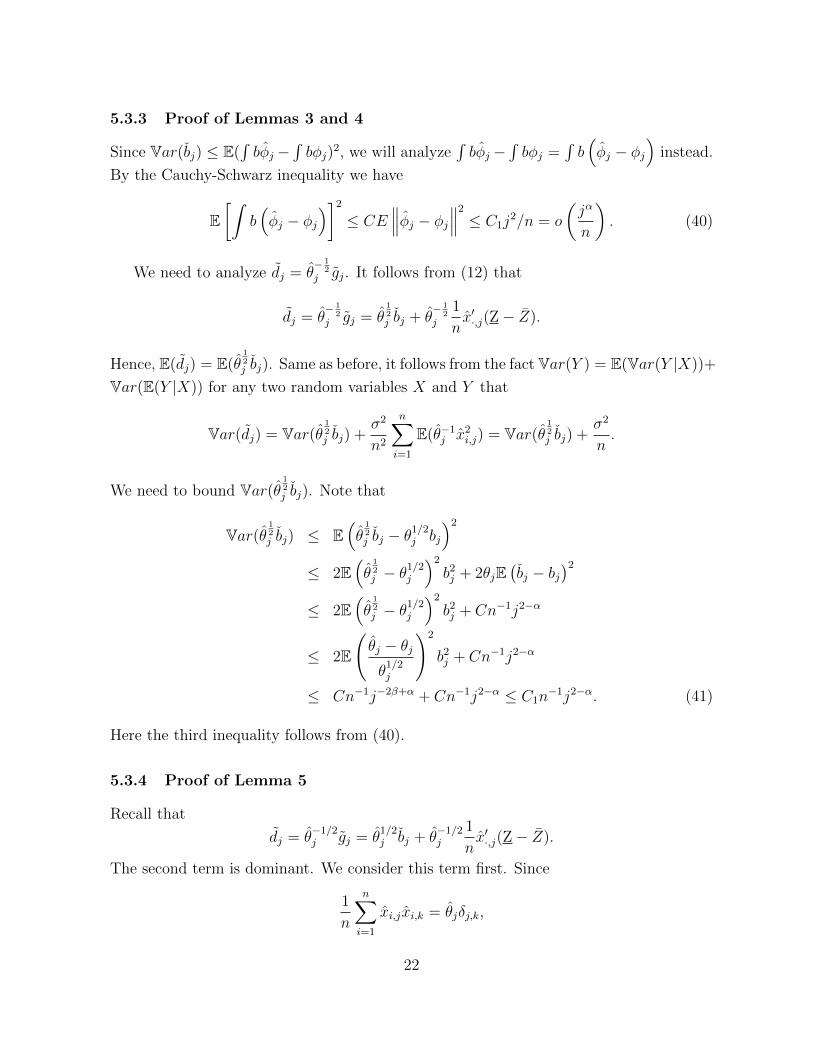
5.3.3 Proof of Lemmas 3 and 4

Since Var(bj) ≤ E(∫bφj −

∫bφj)

2, we will analyze∫bφj −

∫bφj =

∫b(φj − φj

)instead.

By the Cauchy-Schwarz inequality we have

E[∫

b(φj − φj

)]2≤ CE

∥∥∥φj − φj∥∥∥2 ≤ C1j2/n = o

(jα

n

). (40)

We need to analyze dj = θ− 1

2j gj. It follows from (12) that

dj = θ− 1

2j gj = θ

12j bj + θ

− 12

j

1

nx′·,j(Z− Z).

Hence, E(dj) = E(θ12j bj). Same as before, it follows from the fact Var(Y ) = E(Var(Y |X))+

Var(E(Y |X)) for any two random variables X and Y that

Var(dj) = Var(θ12j bj) +

σ2

n2

n∑i=1

E(θ−1j x2i,j) = Var(θ12j bj) +

σ2

n.

We need to bound Var(θ12j bj). Note that

Var(θ12j bj) ≤ E

(θ

12j bj − θ

1/2j bj

)2≤ 2E

(θ

12j − θ

1/2j

)2b2j + 2θjE

(bj − bj

)2≤ 2E

(θ

12j − θ

1/2j

)2b2j + Cn−1j2−α

≤ 2E

(θj − θjθ1/2j

)2

b2j + Cn−1j2−α

≤ Cn−1j−2β+α + Cn−1j2−α ≤ C1n−1j2−α. (41)

Here the third inequality follows from (40).


Recall that

dj = θ−1/2j gj = θ

1/2j bj + θ

−1/2j

1

nx′·,j(Z− Z).

The second term is dominant. We consider this term first. Since

1

n

n∑i=1

xi,jxi,k = θjδj,k,

22

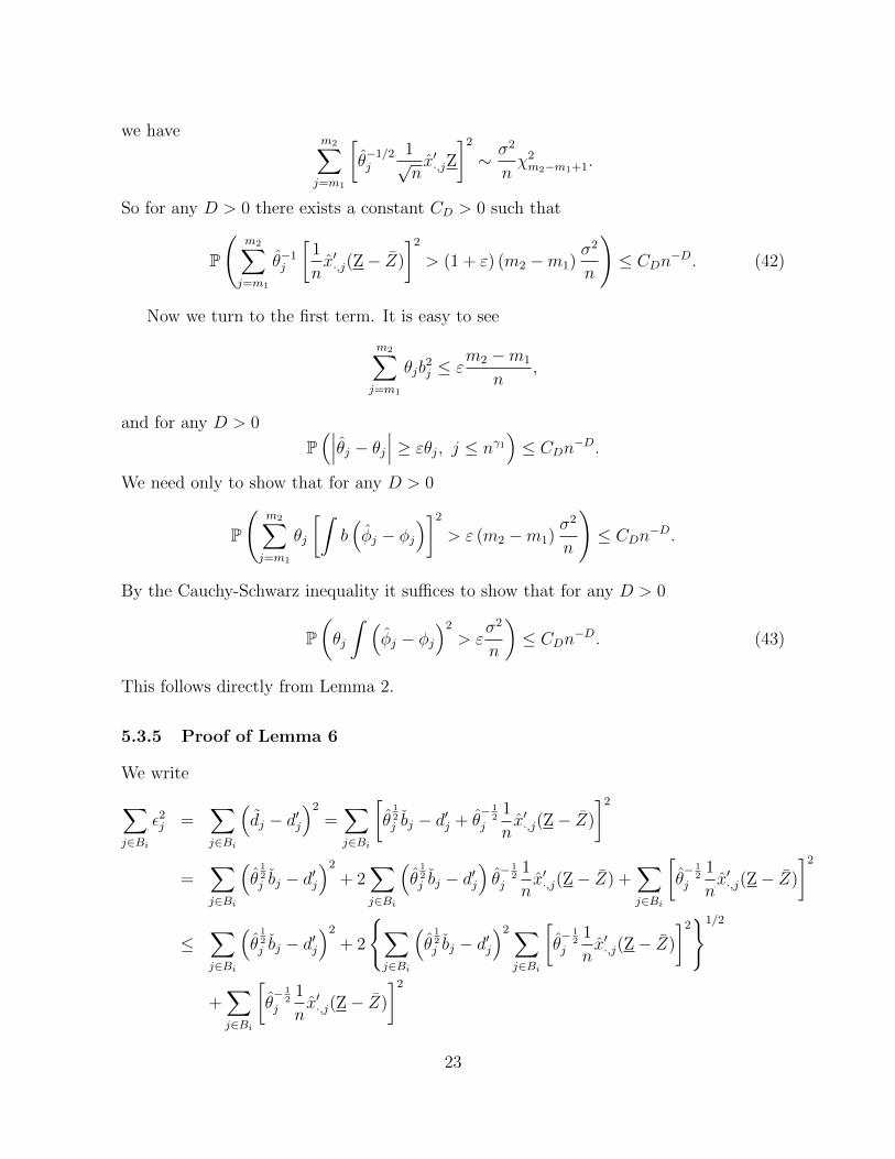
we havem2∑j=m1

[θ−1/2j

1√nx′·,jZ

]2∼ σ2

nχ2m2−m1+1.

So for any D > 0 there exists a constant CD > 0 such that

P

(m2∑j=m1

θ−1j

[1

nx′·,j(Z− Z)

]2> (1 + ε) (m2 −m1)

σ2

n

)≤ CDn

−D. (42)

Now we turn to the first term. It is easy to see

m2∑j=m1

θjb2j ≤ ε

m2 −m1

n,

and for any D > 0

P(∣∣∣θj − θj∣∣∣ ≥ εθj, j ≤ nγ1

)≤ CDn

−D.

We need only to show that for any D > 0

P

(m2∑j=m1

θj

[∫b(φj − φj

)]2> ε (m2 −m1)

σ2

n

)≤ CDn

−D.

By the Cauchy-Schwarz inequality it suffices to show that for any D > 0

P(θj

∫ (φj − φj

)2> ε

σ2

n

)≤ CDn

−D. (43)

This follows directly from Lemma 2.


We write∑j∈Bi

ε2j =∑j∈Bi

(dj − d′j

)2=∑j∈Bi

[θ

12j bj − d′j + θ

− 12

j

1

nx′·,j(Z− Z)

]2=

∑j∈Bi

(θ

12j bj − d′j

)2+ 2

∑j∈Bi

(θ

12j bj − d′j

)θ− 1

2j

1

nx′·,j(Z− Z) +

∑j∈Bi

[θ− 1

2j

1

nx′·,j(Z− Z)

]2

≤∑j∈Bi

(θ

12j bj − d′j

)2+ 2

{∑j∈Bi

(θ

12j bj − d′j

)2 ∑j∈Bi

[θ− 1

2j

1

nx′·,j(Z− Z)

]2}1/2

+∑j∈Bi

[θ− 1

2j

1

nx′·,j(Z− Z)

]223

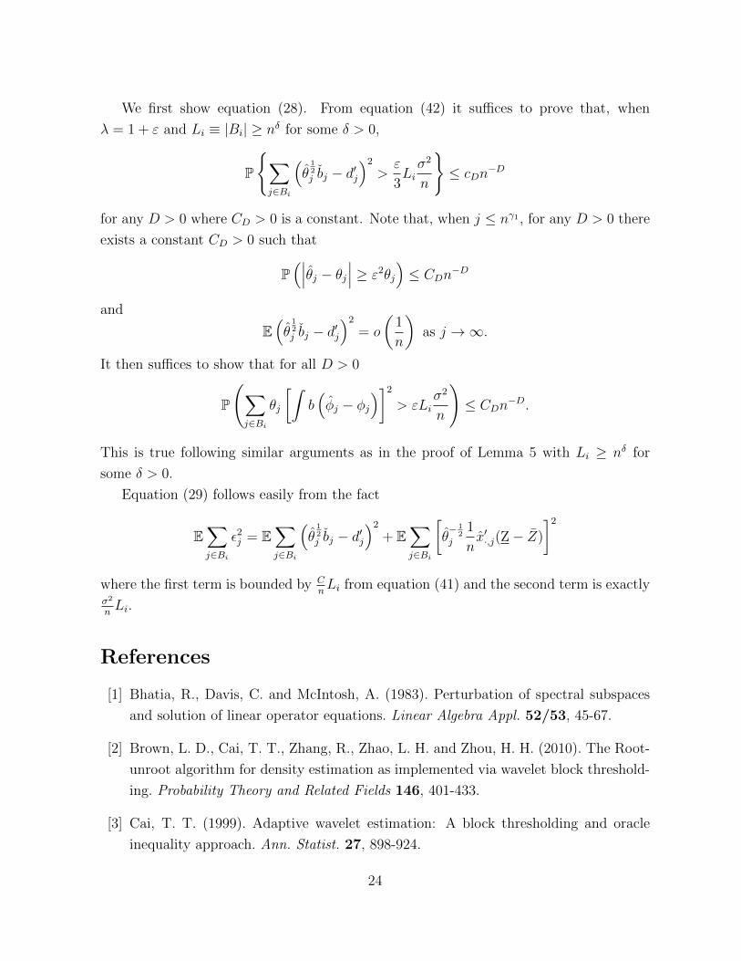
We first show equation (28). From equation (42) it suffices to prove that, when

λ = 1 + ε and Li ≡ |Bi| ≥ nδ for some δ > 0,

P

{∑j∈Bi

(θ

12j bj − d′j

)2>ε

3Liσ2

n

}≤ cDn

−D

for any D > 0 where CD > 0 is a constant. Note that, when j ≤ nγ1 , for any D > 0 there

exists a constant CD > 0 such that

P(∣∣∣θj − θj∣∣∣ ≥ ε2θj

)≤ CDn

−D

and

E(θ

12j bj − d′j

)2= o

(1

n

)as j →∞.

It then suffices to show that for all D > 0

P

(∑j∈Bi

θj

[∫b(φj − φj

)]2> εLi

σ2

n

)≤ CDn

−D.

This is true following similar arguments as in the proof of Lemma 5 with Li ≥ nδ for

some δ > 0.

Equation (29) follows easily from the fact

E∑j∈Bi

ε2j = E∑j∈Bi

(θ

12j bj − d′j

)2+ E

∑j∈Bi

[θ− 1

2j

1

nx′·,j(Z− Z)

]2where the first term is bounded by C

nLi from equation (41) and the second term is exactly

σ2

nLi.

References

[1] Bhatia, R., Davis, C. and McIntosh, A. (1983). Perturbation of spectral subspaces

and solution of linear operator equations. Linear Algebra Appl. 52/53, 45-67.

[2] Brown, L. D., Cai, T. T., Zhang, R., Zhao, L. H. and Zhou, H. H. (2010). The Root-

unroot algorithm for density estimation as implemented via wavelet block threshold-

ing. Probability Theory and Related Fields 146, 401-433.

[3] Cai, T. T. (1999). Adaptive wavelet estimation: A block thresholding and oracle

inequality approach. Ann. Statist. 27, 898-924.

24

[4] Cai, T. T. and Hall, P. (2006). Prediction in functional linear regression. Ann. Statist.

34, 2159-2179.

[5] Cai, T. T., Low, M., and Zhao, L. (2009). Sharp adaptive estimation by a blockwise

method. Journal of Nonparametric Statistics 21, 839-850.

[6] Cardot and Sarda, P. (2006). Linear regression models for functional data. In The

Art of Semiparametrics, pp. 49-66. Physica-Verlag HD.

[7] Cuevas, A., Febrero, M. and Fraiman, R. (2002). Linear functional regression: the

case of fixed design and functional response. Canad. J. Statist. 30, 285-300.

[8] Efromovich, S. Y. (1985). Nonparametric estimation of a density of unknown smooth-

ness. Theory Probab. Appl. 30, 557-661.

[9] Ferraty, F. and Vieu, P. (2000). Fractal dimensionality and regression estimation in

semi-normed vectorial spaces. C. R. Acad. Sci. Paris Ser. I 330, 139-142.

[10] Ferraty, F. and Vieu, P. (2006). Nonparametric Functional Data Analysis. Springer,

New York.

[11] Hall, P. and Horowitz, J. L. (2007). Methodology and convergence rates for functional

linear regression. Ann. Statist. 35, 70-91.

[12] Hall, P. and Hosseini-Nasab, M. (2006). On properties of functional principal com-

ponents analysis. J. R. Statist. Soc. B 68, 109-126.

[13] Hall, P., Kerkyacharian, G. and Picard, D. (1998). Block threshold rules for curve

estimation using kernel and wavelet methods. Ann. Statist. 26, 922-942.

[14] Li, Y. and Hsing, T. (2007). On rates of convergence in functional linear regression.

J. Multivariate Analysis 98, 1782-1804.

[15] Muller, H.-G. and Stadtmuller, U. (2005). Generalized functional linear models. Ann.

Statist. 33, 774-805.

[16] Ramsay, J.O. and Silverman, B.W. (2002). Applied Functional Data Analysis: Meth-

ods and Case Studies. Springer, New York.

[17] Ramsay, J.O. and Silverman, B.W. (2005). Functional Data Analysis, 2nd Edition.

Springer, New York.

25

adaptive functional linear regression via functional ...tcai/paper/adaptive-flr.pdf · adaptive...

Documents