applying functional principal components to structural
TRANSCRIPT

Consiglio Nazionale delle RicercheIstituto di Matematica Applicata
e Tecnologie Informatiche “Enrico Magenes”
REPORT S
G. Alaimo, F. Auricchio, I. Bianchini, E. Lanzarone
Applying Functional PrincipalComponents to Structural
Topology Optimization
17-09

IMATI REPORT Series
Nr. 17-09
April 2017
Managing Editor
Paola Pietra
Editorial Office
Istituto di Matematica Applicata e Tecnologie Informatiche “E. Magenes” Consiglio Nazionale delle Ricerche Via Ferrata, 5/a 27100 PAVIA (Italy) Email: [email protected] http://www.imati.cnr.it
Follow this and additional works at: http://www.imati.cnr.it/reports
Copyright © CNR-IMATI, 2017. IMATI-CNR publishes this report under the Creative Commons Attributions 4.0 license.

IMATI Report Series Nr. 17-09 April 7, 2017
Applying Functional Principal Components to Structural Topology Optimization
Gianluca Alaimo, Ferdinando Auricchio, Ilaria Bianchini, Ettore Lanzarone
_______________________________________________________________________________________________ Copyright © CNR-IMATI, April 2017

Corresponding author: Ettore Lanzarone Istituto di Matematica Applicata e Tecnologie Informatiche “E. Magenes” – CNR Via A. Corti,12 - 20133 Milano e-mail address: [email protected] Gianluca Alaimo Dipartimento di Ingegneria Civile e Architettura, Università di Pavia Via Ferrata, 3 - 27100 Pavia e-mail address: [email protected] Ferdinando Auricchio Dipartimento di Ingegneria Civile e Architettura, Università di Pavia Via Ferrata, 3 - 27100 Pavia e-mail address: [email protected]
Ilaria Bianchini Dipartimento di Matematica, Politecnico di Milano via Bonardi 9 - 20133 Milano e-mail address: [email protected]
_______________________________________________________________________________________________

Abstract
Structural Topology Optimization optimizes the mechanical performance of a structure while satisfying
some functional constraints. Nearly all approaches proposed in the literature are iterative, and the optimal
solution is found by repeatedly solving a Finite Elements Analysis (FEA). It is thus clear that the bottleneck
is the high computational effort, as these approaches require solving the FEA a large number of times. In
this work, we address the need for reducing the computational time by proposing a reduced basis method
that relies on the Functional Principal Component Analysis (FPCA). The methodology has been validated
considering a Simulated Annealing approach for the compliance minimization in a variable thickness
cantilever sheet. Results show the capability of FPCA to provide good results while reducing the
computational times, i.e., the computational time for a FEA analysis is about one order of magnitude lower
in the reduced FPCA space.
Keywords: Structural Topology Optimization; Functional Principal Components Analysis; Finite Element Analysis
_______________________________________________________________________________________________

[page left intentionally blank]

Applying Functional Principal Components
to Structural Topology Optimization
Gianluca Alaimo1, Ferdinando Auricchio1,Ilaria Bianchini2, Ettore Lanzarone3∗
1Universita di Pavia, Department of Civil Engineering and Architecture, Pavia, Italy.2Politecnico di Milano, Department of Mathematics, Milan, Italy
3CNR-IMATI, Milan, Italy
Abstract
Structural Topology Optimization optimizes the mechanical performance of a structure while
satisfying some functional constraints. Nearly all approaches proposed in the literature
are iterative, and the optimal solution is found by repeatedly solving a Finite Elements
Analysis (FEA). It is thus clear that the bottleneck is the high computational effort, as
these approaches require solving the FEA a large number of times. In this work, we address
the need for reducing the computational time by proposing a reduced basis method that
relies on the Functional Principal Component Analysis (FPCA). The methodology has been
validated considering a Simulated Annealing approach for the compliance minimization in
a variable thickness cantilever sheet. Results show the capability of FPCA to provide good
results while reducing the computational times, i.e., the computational time for a FEA
analysis is about one order of magnitude lower in the reduced FPCA space.
Keywords
Structural Topology Optimization; Functional Principal Components Analysis; Finite Ele-
ment Analysis.
∗Corresponding author:
Ettore Lanzarone
1

1. Introduction
Structural optimization techniques aim to obtain optimized performance from a structure
while satisfying several functional constraints, e.g., the total mass to employ or stress limits.
The need for optimized solutions in structural applications has increased over the years
and has become nowadays fundamental, due to the limited availability of commodities, the
environmental impact, the market competition, and the new manufacturing processes, e.g.,
the 3D-printing.
Three main categories can be distinguished in the wide class of structural optimization
methodologies, i.e. size optimization, shape optimization and topology optimization. We
focus on the Structural Topology Optimization (STO) of continuum structures, whose aim
is to produce an optimized structural component by determining its best mass or volume
distribution in a given design domain. Differently from the other alternatives, which deal
with predefined configurations, STO design can attain any shape within the domain.
STO is essentially treated as a constrained minimization or maximization problem. Sev-
eral approaches and algorithms have been proposed for STO, as documented by the huge
literature available on the topic (Huang & Xie, 2010; Hassani & Hinton, 2012; Bendsøe &
Sigmund, 2013; Sigmund & Maute, 2013; Van Dijk et al., 2013; Rozvany & Lewinski, 2014;
Rozvany, 2014). The main distinction is between gradient-based and non-gradient-based
approaches; however, nearly all of the algorithms are iterative, and the optimal solution is
found by repeatedly performing a structural Finite Elements Analysis (FEA) which involves
the solution of the equilibrium equations of the problem under study.
On the one hand, such iterative approaches are powerful, as they allow to determine
optimized solutions in a variety of situations without additional assumptions. On the other
hand, the bottleneck of such approaches is the high computational effort, as they require to
perform the FEA a large number of times, as reported in Bendsøe & Sigmund (2013). As
an example, in a minimum compliance problem (see Sect. 2.1), up to the 97% of the total
computational time may be employed in the numerical solution of the equilibrium equations
(Borrvall & Petersson, 2001).
In this perspective, the need for reducing the computational time of performing the
FEA instances in STO, especially for large problems and 3D applications, is crucial. In
this work, we address this issue by proposing a reduced basis method that relies on the
Functional Principal Component Analysis (FPCA), namely the functional counterpart of
the classical Principal Component Analysis (PCA), in order to improve the efficiency of the
FEA employed in STO.
Coupling FPCA with structural FEA allows to reduce the dimensionality of the structural
problem, i.e., the number of equilibrium equations to be solved. In this way, a substantial
saving of the computational time required could be achieved at each iteration, without any
appreciable loss of accuracy. Thus, the advantages in terms of time reduction for STO could
2

be relevant.
To the best of our knowledge, the idea of coupling FPCA and FEA has been exploited
only once in the literature (Bianchini et al., 2015). However, in the cited reference, the
authors coupled FPCA and FEA for the purpose of uncertainty quantification, in order to
estimate the probability distribution of some output random variables (e.g., the displacement
in a given direction) in the presence of stochastic input parameters (e.g., the Young modulus).
The novelty of the present work is to couple FPCA and FEA for an optimization purpose,
which has been never considered before.
Briefly, at each iteration of the STO, we convert the FEA problem into a reduced one
by projecting into a smaller space by means of a data-driven reduced FPCA basis. The
reduced problem is solved and, if the error associated with the solution is below a given
threshold, the reduced solution is accepted; otherwise, the original FEA problem is solved
and the complete solution is also used for updating the FPCA basis.
In the present work, we employ the proposed methodology along with a Simulated An-
nealing (SA) approach, as an example of iterative non-gradient based algorithm. However,
we underline that the proposed FPCA methodology can be used along with any iterative
algorithm employed in STO. More in general, the discussion on the most suitable algorithm
for STO is still open (Sigmund, 2011); anyway, this is not the focus of our work.
The paper is structured as follows. A literature review on STO and the approaches to
reduce the dimensionality and the computational effort in FEA is presented in Sect. 2. The
considered problem and the proposed methodology are described in Sect. 3. Then, the test
case used to validate the approach is shown in Sect. 4, while the computational analyses
and the related results are presented in Sect. 5. The discussions and the conclusion of the
work are finally drawn in Sect. 6.
2. Literature review
2.1. Structural Topology Optimization (STO)
As highlighted in Sect. 1, a huge literature on STO is available regarding theoretical
aspects, numerical methods and applications.
Collections of lectures dealing with several aspects of STO and optimality criteria are
edited by Rozvany & Lewinski (2014) and Rozvany (2014). Review papers focusing on
level-set methods, evolutionary approaches and established methods of structural topology
optimization are also available (Rozvany, 2009; Huang & Xie, 2010; Sigmund & Maute,
2013; Van Dijk et al., 2013). The fundamentals of the material distribution method and its
extension to anisotropic materials are presented in Bendsøe & Sigmund (2013), considering
dynamic and buckling problems as well as the design of truss structures. Hassani & Hinton
(2012) treated STO with periodic material distribution, for which macro constitutive models
are derived through suitable homogenization techniques.
3

A widely used methodology in STO is represented by the density based approach, in
which the design domain Ω is discretized into a set of N elements and the density parameters
ρi associated to each element i (i = 1, . . . , N) are optimized. This method gained popularity
because it does not require domain re-meshing at each iteration (Zegard & Paulino, 2016).
Following this approach, the elastic modulus Ei of element i is related to its density
ρi according to the modified Solid Isotropic Material with Penalization (SIMP) scheme as
follows (Bendsøe, 1989; Zhou & Rozvany, 1991; Sigmund, 2007):
Ei (ρi) = Emin + ρpi (E0 − Emin) , ∀i (1)
where E0 is the elastic modulus of the solid material, Emin is the lower limit of the elas-
tic modulus (introduced to overcome computational issues in the presence of zero-stiffness
elements while solving the equilibrium equations), ρi ∈ [0, 1], and p ≥ 1 is a penalization
factor. Higher values of p make less convenient to use intermediate values of density between
solid (ρi = 1) and void (ρi = 0).
SIMP method with no penalization (p = 1) yields a linear relation between Ei and ρi,
giving the so-called variable thickness sheet problem for which the solution is unique in the
case of stiffness maximization (Petersson, 1999).
Discrete elements i for STO usually coincide with the mesh used for numerically solving
the FEA problem, even though they are theoretically independent. As a consequence, the
optimized solution depends on the level of the mesh refinement. Indeed, the introduction of
finer meshes (and consequently of smaller elements in a structure with fixed domain) leads
to a material distribution in the form of micro-structure, which increases the efficiency of the
optimized structure. In fact, microstructure-like material distributions lead to an improved
use of the material. However, even though a fine mesh is required to properly solve the FEA
problem, it is not always possible to build features below a certain scale from a technical
feasibility viewpoint.
To overcome this issue, relaxation or restriction methods can be used to uncouple the
discretization into elements from the mesh(Bendsøe & Kikuchi, 1988; Ambrosio & Buttazzo,
1993; Haber et al., 1996; Sigmund, 1997; Bourdin, 2001; Bruns & Tortorelli, 2001; Xu et al.,
2010). The rationale behind these methods is the reduction of the space of the admissible
designs by imposing weak constraints or restrictions on the density variation; thus, material
configurations resembling micro structures can be avoided.
2.2. Dimensionality reduction in FEA
Dimensionality reduction in FEA is based on spectral decomposition of the covari-
ance/correlation structure of the displacement field u(x, ρ), where x denotes the coor-
dinates of a point in the considered domain Ω and ρ represents a vector of parameters, e.g.,
densities, characterizing the FEA instance at each given iteration of the STO optimization.
4
Spectral methods are widely adopted in the literature (Ghanem & Spanos, 1991). Among
them, PCA and Karhunen-Loeve expansion are those frequently applied to FEA; the first
considers the covariance matrix, while the latter the spectrum of the correlation matrix. Both
of them require the knowledge of the covariance structure of u(x, ρ), and in particular of the
corresponding eigenfunctions. The covariance structure is estimated from a set of already
available solutions of the FEA problem, i.e., the basis depends on the covariance function
of the solution process and the approach is data dependent.
Alternatively, the Proper Generalized Decomposition (PGD) represents an a priori ap-
proach, which does not rely on previous FEA solutions (Nouy, 2010; Chinesta et al., 2011).
Indeed, the solution is approximated a priori by minimizing a norm of the error with re-
spect to the Karhunen-Loeve decomposition, leading to a pseudo eigenproblem (details can
be found in Chinesta et al. (2013)).
Finally, there exist other well-established methods in the literature, based on alternative
expansions, which involve a basis of known random functions with deterministic coefficients,
namely the Polynomial Chaos Expansion (PCE). The latest methodological developments
of PCE can be found in Panayirci & Schueller (2011) and Yu et al. (2012), while recent
applications can be found in different fields, e.g., hydrology (Sochala & Le Maıtre, 2013),
piezoelectric materials (Umesh & Ganguli, 2013), and dosimetry to study the human expo-
sure to magnetic fields (Liorni et al., 2014).
Resuming PCA, it is widely used in statistics to look at the covariance structure of
multivariate and complex data (Johnson & Wichern, 1992; Ramsay & Silverman, 2005). In
the context of mechanical systems, the method turns out to be useful for characterizing the
dynamic behavior and to reduce the order of linear and non-linear systems (Kerschen et al.,
2005). Thus, PCA has been successfully applied in a variety of problems, e.g., aeroelastic
problems, damage detection, dynamic characterization, and modal analysis. It was initially
applied in solid mechanics (Sirovich, 1987); then, it has been employed in structural non-
linear dynamics (Dulong et al., 2007) and to analyze vibro-impact systems (Ritto et al.,
2012).
In particular, in Dulong et al. (2007), PCA has been employed for real-time analysis of
non-linear mechanical behaviors. Interestingly for our work, the approach is divided into
a training phase and a real-time phase. In the training phase, several FEA solutions are
computed under different load values; then, PCA is used in the real-time phase to reduce
the amount of data to store and the computational time.
Moreover, it is worth mentioning that, in the context of stochastic FEA, Florentin & Dıez
(2012) introduced an adaptive strategy to build a reduced basis in which, at each Monte
Carlo iteration, the distance between the FEA solution and the solution obtained in the
reduced space is checked. If the distance is larger than a threshold, the reduced solution
is discarded and the complete solution is computed and added to the current basis. Their
proposed approach measuring the distance between the solutions is interesting; however, the
5

adopted reduced basis is not orthogonal, thus leading to an ill-conditioned matrix for the
basis change.
All of the works in which the decomposition exploits the covariance matrix are based on
the standard PCA, where data are treated as multivariate vectors, thus merely considering
the displacements of the nodes of the mesh. On the contrary, the FPCA (Ramsay & Silver-
man, 2005; Horvath & Kokoszka, 2012) has been only adopted in Bianchini et al. (2015), to
build the reduced basis in the context of stochastic FEA. The approach in Bianchini et al.
(2015) relies on the idea of evaluating the distance between the complete FEA solution and
the solution obtained in the reduced space to assess whether to keep or to discard a reduced
solution (as in Florentin & Dıez (2012)); however, a data-driven basis is built according to
the FPCA.
To conclude, PCA has been already adopted in the literature to address optimization
problems (an overview of several optimization problems related to PCA under various ge-
ometric perspectives can be found in Reris & Brooks (2015)). However, to the best of our
knowledge, the functional counterpart (FPCA) that we are here proposing has been never
coupled with FEA in the context of structural optimization, and only once in the context
of stochastic FEA (Bianchini et al., 2015).
3. Proposed methodology
We first describe in Sect 3.1 the addressed STO problem; then we present the approach
proposed to solve such a problem. The core of the approach (i.e., FPCA applied to FEA)
is detailed in Sect. 3.2, while the iterative SA algorithm for this case is presented in Sect.
3.3. Finally, precautions to take for properly employing the FPCA basis are highlighted in
Sect. 3.4.
3.1. Addressed problem
We refer to a linear elastic structural problem in a continuous domain Ω, whose goal is
to find the displacement field u (x) ∈ L2 (Ω) that minimizes the overall elastic energy (or
compliance) C, which depends on the displacement u (x) as follows:
C =1
2
∫Ω
f (x)u (x) dx (2)
where f (x) is the imposed force field.
We consider the variable thickness sheet problem (see Sect. 2.1). We discretize the
domain into elements i (i = 1, . . . , N) with the same area, and each elastic modulus Eilinearly depends on the density ρi as Ei (ρi) = ρiEmat, where ρi ∈ [0, 1] and Emat is the elastic
modulus of the solid material when the thickness assumes its maximum value (ρi = 1). To
overcome computational issues in case of zero-stiffness elements, we redefine the range of
6

each ρi as [ρmin, 1], with ρmin > 0, which is equivalent to what presented in (1). The goal of
our STO is to find the best vector ρ = [ρ1 . . . ρN ] that minimizes C (ρ), given one or more
constraints on the ρi values. In the following, as constraint, we impose a fixed value ρ∗ to
the mean ρi over the elements.
Thus, the nominal problem is:
minimize C (ρ)
s.t. Linear elastic problem in function of ρ∑N
i=1 ρi
N= ρ∗
ρmin ≤ ρi ≤ 1, i = 1, . . . , N
Actually, we refer to the discretized counterpart of (2), namely:
C = u′ K u (3)
with Ku = F , where u, F and K are the discretized displacement vector, force vector and
stiffness matrix, respectively. Symbol ′ denotes matrix transposition.
Moreover, as for the densities ρi, we add the well-known linear density filter (Sigmund,
2007), considering the following filtered densities ρi:
ρi =
∑j∈Ni
h(yj)Ajρj∑
j∈Ni
h(yj)Aj
(4)
Aj and xj are the area and the center location of element j, respectively, while yj appearing
in the formula is a transformed vector for the coordinates such that yj = Γxj. Ni is the
neighborhood of element i, defined as:
Ni = k : ‖yk − yi‖ < R
and h(yj)
= R −∥∥yj − yi∥∥ is a linear weight function. Matrix Γ allows us to consider
different shapes for the neighborhood of the elements. In this way, the elastic modulus Eiis redefined as:
Ei (ρi) = ρiEmat (5)
Thus, the addressed problem is stated as follows:
minimize C (ρ) (6)
7

s.t.
Discretized linear elastic problem in function of ρ
ρi =
∑j∈Ni
h (Γxj)Ajρj∑j∈Ni
h (Γxj)Aj∑Ni=1 ρi
N= ρ∗
ρmin ≤ ρi ≤ 1, i = 1, . . . , N
(7)
with ρ = [ρ1 . . . ρN ]′.
3.2. Building a reduced basis via FPCA
The methodological content of this section is based on the FPCA reduction approach
developed in Bianchini et al. (2015); the interested reader can refer to such a reference
for further details. However, as mentioned, the objective of Bianchini et al. (2015) was to
investigate the variability of a certain output quantity of interest given that some mechanical
parameters are random. Here, on the contrary, the optimization problem does not include
any randomness/variability, since we are looking for the (deterministic) configuration of
parameters that leads to the optimal output. This difference does not prevent us from
exploiting the FPCA reduction approach as in Bianchini et al. (2015), even though some
precautions are needed (as discussed in Sect. 3.4).
3.2.1. FPCA for FEA
Let U(Θ) = u(x,ρ),ρ ∈ Θ ∈ L2 (Ω) be the solutions space of the structural prob-
lem, with Θ = [ρmin, 1]N . The goal of the FPCA is to describe U(Θ) through an optimal
orthonormal basis.
For this purpose, we need M realizations of the solution, obtained with as many values
ρm (m = 1, . . . ,M) of the parameter vector ρ; of course, the bigger M is, the more accurate
the procedure will be.
By assuming that M is large enough, the subspace spanned by the solutions
u(x,ρm),m = 1, . . . ,M
approximates U(Θ). Thus, by applying FPCA to these solutions, we may estimate the K
orthonormal basis functions that optimally approximate U(Θ), where K is a fixed integer
value with 1 6 K 6M .
Indeed, FPCA is a method to build an approximation of the set of solutions. Let us de-
note by vm(x) the solution u(x,ρm) and by vm(x) the corresponding approximate solution.
8

The approximation takes the following form:
vm(x) =K∑k=1
fmk ξk(x)
where ξk(x), k = 1, . . . , K are the orthonormal principal functions and fmk the principal
component scores corresponding to the m-th solution, which are defined as:
fmk =
∫Ω
vm(s) ξk(s) ds k = 1, . . . , K
The data-driven basis we are considering collects the principal functions. This basis is
optimal, as the K functions ξk(x), k = 1, . . . , K achieve the minimum of the following
error measure χ, given the M observed functions vm(x),m = 1, . . . ,M:
χ =M∑m=1
‖vm − vm‖2L2 =
M∑m=1
∫Ω
(vm(s)− vm(s))2 ds
In other words, the basis minimizes the sum of the L2 reconstruction errors over the M data.
From an operative viewpoint, the elements of the basis solve a particular eigenvalue prob-
lem which involves the covariance operator. Let us considerM functions vm(x),m = 1, . . . ,Mwith a null cross-sectional mean, i.e.,
1
M
M∑m=1
vm(x) = 0
Then, the associated (empirical) covariance function is defined as:
V(s, t) =1
M
M∑m=1
vm(s)vm(t)
and the corresponding covariance operator as:
Vξ : ξ(·) 7→∫
Ω
V(·, t)ξ(t)dt
Hence, each principal component turns out to solve the following eigenproblem:
Vξ(x) = γξ(x) (8)
and the FPCA can be equivalently expressed as the eigenanalysis of the covariance operator
V. This characterization helps us in building the basis, as explained in the next section.
9

3.2.2. Creation of the reduced basis
We start from M solutions u1 (x) , . . . ,uM (x) obtained solving complete FEA problems
for different values of ρ, and we define the matrix
U = [u (ρ1)− u, . . . , u (ρM)− u]′
where u (ρm) is the vector containing the displacements in all of nodes of the FEA mesh
(ordered as the displacements of the first node, then of the second node, and so on) and u
is the sample mean
u =1
M
M∑m=1
u (ρm)
Thus, the dimension of U is M × 2L, where L is the number of elements of the mesh.
We have to find out the orthonormal basis based on the functional principal components
of matrix U. We suggest to use the method of snapshots (Sirovich, 1987; Volkwein, 2011)
to determine the basis: if 2L > M , which is certainly our case, the basis of rank K is
determined as follows:
• define Y = (UW1/2)′ with
W = [wb1b2 ]
[∫φb1(x)φb2(x)dx
]where φk(·) are the finite element functions;
• solve the eigenvalue problem
Y′Yvk = λkvk k = 1, . . . , K
where λk are in descending order;
• set
ξk =1√λkU′vk k = 1, . . . , K.
The projection into the reduced space of dimension K can be done using the following
matrix:
Urb = [ξ1, . . . , ξK ] .
Finally, we have to choose the value of K. We adopt a method based on the maximum
eigenvalue λmax, i.e., we retain all of the eigenfunctions corresponding to an eigenvalue λksuch that λk > Λλmax, where Λ typically assumes small values, e.g., 10−4 (Dulong et al.,
2007).
10

3.2.3. Reduced FEA problem
We employ the reduced basis because, at each iteration g of the optimization method
(e.g., the SA adopted in this work), we solve a reduced problem, which is much less compu-
tationally demanding as the solution is obtained in the subspace spanned by the principal
components.
The complete FEA problem corresponding to the linear elastic problem requires to solve
Kgug = F (9)
where Kg is the stiffness matrix for realization ρg.
On the contrary, the reduced problem is obtained by projecting the problem into the
subspace spanned by the K principal components:
U′rbKgured,g = U′rbF , (10)
with ured,g = ug + UrbU′rbug = u + Urbag and ag = U′rbug ∈ Rk. Thus projection (10)
becomes:
U′rbKgUrbag +U′rbKgug = U′rbF
Summing up, for each iteration/realization g, the reduced problem turns out to be the
following: Krbag = F rb
ured,g = Urbag
ug = ug + ured,g
(11)
with:
• Krb = U′rbKgUrb;
• F rb = U′rbF −U′rbKgug = U′rb (F −Kgug).
Obviously, the solution ug of (11) is computationally cheaper than the solution obtained
when solving a complete FEA problem, but it is only an approximation. To monitor the
approximation error, we compute at each iteration g the residual ered,g = Kgured,g −F and
consider its quadratic norm
errg = ‖ered,g‖2L2 = e′red,gWered,g
as an estimate for the error.
We check whether errg < tol, where tol is a tolerance value defined by the user. If the
condition is satisfied, we keep the reduced solution for iteration g and go ahead with the next
iteration g + 1. Conversely, if the condition is not satisfied, we discard the reduced solution
and solve the full problem. The complete solution of the full problem is kept for iteration
11

g, and it is also used as a further realization to update the basis. The newly updated basis
replaces the previous one for all of the following iterations of the algorithm, until a new
update is required.
Anyway, the construction of the reduced FPCA basis requires several FEA solutions;
thus, at the first M∗ iterations, the complete FEA problem is directly solved.
3.3. Simulated annealing algorithm
We employ the classical framework of the SA iterative algorithm, in which the optimal
solution S∗ is refined iteration by iteration (Henderson et al., 2003). Below, we briefly recall
the framework and we detail the main points of our implementation.
In general, at each iteration g of the algorithm, a new solution Sg is computed based
on a given value ρg. If the newly provided solution Sg has a better value of the objective
function than the current optimal solution S∗, new solution Sg replaces the current S∗, and
the value ρg+1 for the next iteration is computed based on the current one ρg. Otherwise,
the provided solution Sg can be accepted with a probability πg. If accepted, once again Sgreplaces the current S∗, and the value ρg+1 is computed based on ρg. If not accepted, the
solution Sg is not considered and the value ρg+1 is computed based on that of the current
optimal solution ρ∗. The solution S∗ at the end of the iterations is the optimal solution
provided by the SA.
In our work, each solution Sg refers to problem (7), once a value ρg is fixed. To complete
the description of the algorithm, we must provide the approach to compute the next value
ρg+1 while respecting the mean ρ∗, the rule to compute probability πg, the initialization of
the algorithm, and the termination criteria.
As for the next value ρg+1, it is built by first adding a discrete Gaussian random field
with null mean to the current density field. Then, values outside of the range [ρmin, 1]
are replaced with the closest value in the range, and the resulting field is normalized to
respect that the mean value is ρ∗. The Gaussian field is generated at each iteration, while
its covariance matrix is updated every ggauss iterations, to start from highly variable fields
to highly correlated ones.
Indeed, each element of the covariance matrix is given by σed(yi,yj)φg , where d(yi,yj
)is
the Euclidean distance between the transformed coordinates yi and yj of elements i and j,
respectively, and φg is as follows:
φg = φfinal − (φfinal − φinit) e−gstart/Tgauss
where gstart represents the first value of g within the group of ggauss iterations, and φfinal <
φinit.
Concerning πg, it is based on a cooling schedule, i.e., a strictly monotonic decreasing
temperature function T (g). In our case, we consider the following form:
T (g) = Tmaxe−g/Tsa
12
Then, πg is given by:
πg = e−Cg−C∗
T (g)
where Cg and C∗ refer to the objective function (compliance) values for Sg and S∗, respec-
tively. To evaluate whether to accept a worst solution Sg with Cg > C∗, a random number
ηg uniformly distributed between 0 and 1 is generated; if ηg < πg, then the solution is ac-
cepted. According to the SA framework, accepting a worst solution becomes less likely while
g increases, as T (g) monotonically decreases with g.
Finally, the algorithm is initialized considering a vector ρ1 in which all elements are equal
to ρ∗, while it is terminated after a maximum number G of iterations or when the solution
freezes. The latter, according to the SA framework, occurs when the current optimal solution
S∗ is not updated in the last gf iterations and T (g) is below a given value Tf .
The adopted values of all parameters are reported in the computational analyses (Sect.
5.1).
3.4. Making the basis adaptive
The two ingredients introduced in Sect. 3.2 and 3.3 are combined to build an algorithm
that efficiently solves the STO. Thus, the goal of the reduced basis is to solve an optimization
problem whose characteristics vary along with the iterations g of the optimization.
In particular, the value of ρg changes at each iteration, and after several iterations the
analyzed FEA problem can be strongly different from the previous ones. As a consequence,
we need a basis that follows the changes happening along with the iterations.
For this reason, when an update of the basis is required (because errg ≥ tol), the new
basis is built considering only the last solutions obtained solving a complete FEA problem.
In particular, we consider the last M∗ solutions, where M∗ coincides with the number of the
initial complete solutions (end of Sect. 3.2.3).
In this way, we get rid of the old solutions that are likely to be very different from the
current one, and thus not useful to describe the space U(Θ) in the neighborhood of the
current point. In the absence of such riding, the dimension of the reduced problem could
be uselessly higher, because of including additional variability related to conditions very far
from those currently under investigation. Moreover, including the useless variability, the
error related to the reduced problem could increase.
4. Test case
We validate the proposed approach dealing with one of the classical problems encountered
in STO, i.e., the compliance minimization for a variable thickness cantilever sheet.
The cantilever consists of a rectangular domain Ω (dimension b × h) with Dirichlet
boundary conditions on one of the sides. Moreover, as load, we either consider a constant
body force f d or a concentrated force f c applied in the middle of the side opposite to the
13

one with Dirichlet boundary conditions. The domain, together with the Dirichlet conditions
and the two alternative loads, is sketched below.
f df ch
b
The setting for the tested cases is: Ω = (0, 200) × (0, 40); either f d = (0,−0.1) or
f c = (0,−10); Poisson’s ratio ν = 0.3; Emat = 2000; ρmin = 0.05.
We adopt a standard FEA discretization to solve the problem, based on triangular bi-
linear approximations into a standard principle of virtual work approximation (Zhu et al.,
2005; Hughes, 2012), where n is the number of intervals between nodes per each side of the
domain.
As for ρi, we discretize the domain into N rectangular elements, each one involving two
triangular regions of the mesh; thus, L = 2N and n =√N .
Finally, as for the density filter, we adopt R = 2 the following diagonal matrix Γ:
Γ =
[nb
0
0 nh
]so as to have an elliptic neighbor region for (4), whose semiaxes are proportional to the size
of the elements in that direction.
5. Computational analyses
We first consider one mechanical condition to evaluate the impact of the FPCA param-
eters (Sect. 5.1). Then, fixing these parameters to a suitable value, we investigate several
mechanical conditions to analyze the STO outcomes (Sect. 5.2). Finally, in the same section,
we compare our outcomes with a literature benchmark.
All tests have been run on a Server with processor X86-64 AMD Opteron 6328 and 64GB
of dedicated RAM.
5.1. Impact of FPCA parameters
These analyses are conducted under concentrated force with ρ∗ = 0.5. The analyses refer
to the impact of n, tol, Λ and M . In particular, 3 levels for n (50, 70 and 90), 3 levels for
tol (5%, 7.5% and 10%), 2 levels for Λ (10−7 and 10−4) and 2 levels for M∗ (30 and 50) are
considered.
The other SA parameters are fixed as follows: G = 2000; Tmax = 0.0004; Tsa = 1000;
Tf = 10; gf = 2000 (the latter two values are set to prevent early freezing). Finally,
14

the additional parameters for the Gaussian field are as follows: ggauss = 50; σ = 0.0005;
φinit = 250/n; φfinal = 0.025/n; Tgauss = 500.
All tests are reported in Table 1 together with the main outcomes, i.e., the objective
function C, the mean computational time to run a complete FEA, the number of rejections
of the reduced FEA solution (because errg ≥ tol), the mean computational time to run a
reduced FEA, the mean time to create a new basis, and the maximum number K of vectors
in the basis along with the iterations.
Results clearly show that the computational time required by the reduced FEA is one
order of magnitude lower than the time required by the complete FEA, and that the differ-
ence grows with n. Moreover, the time to compute the basis is about one-fourth of the time
required by the complete FEA.
Details are reported in Figure 1. Plots show that the time required by the complete FEA
strongly increases with n, while on the contrary the increasing of the time required by the
reduced FEA is negligible; thus, this dramatically increases the difference between the times
while n increases. Also the time for creating the basis increases, but again the difference
between the time for the complete FEA and the time for computing the basis increases with
n. Results are retained while varying the other parameters, e.g., parameter tol as in the
three plots of Figure 1.
Moreover, it is worth noting that the other outcomes are about the same while varying
n; in particular, the reached objective function and the number of rejections do not seem to
be affected by n.
As expected, the number of rejections varies along with tol, while it only marginally
depends on other parameters (see Figure 2a as example) showing only a small reduction
from M∗ = 30 to M∗ = 50. Also the objective function C varies with tol, as expected, as
higher tol values increase the error associated with the FEA solutions, thus resulting in an
error associated with the objective function C.
Anyway, the variation of the objective function C is limited and below an approximation
universally accepted for FEA methods. In particular, by comparing the solutions in Table
1 with the corresponding ones without reduced basis (i.e., when tol = 0% and the reduced
solution is never exploited), errors are below the 3% in the majority of cases.
A trade-off is required; in our case we consider tol = 7.5% as the optimal choice because
it gives limited variations of objective functions C with respect to tol = 0%, and because the
largest reduction in the number of rejections is observed between tol = 5% and tol = 7.5%.
As for the impact of Λ, we observe that with Λ = 10−7 the maximum number K of
vectors in the basis along with the iterations is always equal to M − 1, meaning that all
eigenvectors are always included. On the contrary, with Λ = 10−4, a lower number of vectors
15

Input Outcomes
parameters Objective Mean time Number Mean time Mean time Max
function complete of reduced create K
n tol Λ M∗ C FEA [s] rejections FEA [s] basis [s] iter.
50 0.0% – – – – 14.400 0.08512 – – – – – – – – –
50 5.0% 10−7 30 14.444 0.08321 776 0.00531 0.02354 29
50 7.5% 10−7 30 14.747 0.09130 275 0.00491 0.02263 29
50 10.0% 10−7 30 14.862 0.08900 147 0.00415 0.02167 29
50 5.0% 10−4 30 14.431 0.11150 1054 0.00199 0.01781 21
50 7.5% 10−4 30 14.651 0.11062 338 0.00148 0.01599 17
50 10.0% 10−4 30 14.891 0.11201 157 0.00117 0.01602 14
50 5.0% 10−7 50 14.457 0.09603 778 0.00751 0.05052 49
50 7.5% 10−7 50 14.697 0.10351 299 0.00716 0.04851 49
50 10.0% 10−7 50 14.582 0.10722 174 0.00645 0.04515 49
50 5.0% 10−4 50 14.408 0.10171 1114 0.00219 0.03012 23
50 7.5% 10−4 50 14.578 0.11304 472 0.00208 0.02881 22
50 10.0% 10−4 50 14.887 0.10381 222 0.00115 0.02745 8
70 0.0% – – – – 14.472 0.21073 – – – – – – – – –
70 5.0% 10−7 30 14.640 0.20505 791 0.01255 0.05190 29
70 7.5% 10−7 30 14.849 0.23546 265 0.01312 0.05478 29
70 10.0% 10−7 30 15.007 0.22744 163 0.01239 0.05317 29
70 5.0% 10−4 30 14.551 0.20557 1084 0.00412 0.03451 23
70 7.5% 10−4 30 14.832 0.20600 299 0.00271 0.02948 12
70 10.0% 10−4 30 18.168 0.20656 80 0.00234 0.02889 5
70 5.0% 10−7 50 14.535 0.21838 876 0.01693 0.10878 49
70 7.5% 10−7 50 14.634 0.24926 310 0.01854 0.12620 49
70 10.0% 10−7 50 14.847 0.24915 172 0.01435 0.09257 49
70 5.0% 10−4 50 14.557 0.20208 1143 0.00403 0.05726 25
70 7.5% 10−4 50 15.025 0.19835 387 0.00258 0.05104 11
70 10.0% 10−4 50 15.166 0.20014 258 0.00215 0.04994 6
90 0.0% – – – – 14.495 0.35333 – – – – – – – – –
90 5.0% 10−4 30 14.682 0.36901 973 0.00735 0.06166 21
90 7.5% 10−4 30 16.050 0.36560 212 0.00434 0.05751 5
90 10.0% 10−4 30 15.707 0.36508 117 0.00414 0.05663 5
Table 1: Tested cases for concentrated force with ρ∗ = 0.5.
16

Figure 1: Mean time to run a complete FEA, to run a reduced FEA, and to create the basis as a function
of n for tol = 5% (a), tol = 7.5% (b) and tol = 10% (c); other parameters are Λ = 10−4 and M∗ = 30.
17

Figure 2: Number of rejected reduced FEA solutions (a) and objective function C (b) as a function of tol,
for Λ = 10−7 or Λ = 10−4, and M∗ = 30 or M∗ = 50; n = 50 in all cases.
18

Figure 3: Objective function along with the iterations for concentrated force, ρ∗ = 0.5, tol = 7.5%, Λ = 10−4
and M∗ = 50.
is included. This happens with both M∗ = 30 and M∗ = 50. As all other outcomes do not
change with Λ, we consider the simplest case in the following analyses, i.e., Λ = 10−4 and
M∗ = 50.
5.1.1. Convergence of the simulated annealing
Even though the SA employed in the STO is not the core of our work, we verify the
convergence of the algorithm in order to rely on the obtained results.
Figure 3 shows the objective function along with the 2000 iterations for the same case
of concentrated force with ρ∗ = 0.5, in which the above selected parameters are taken (i.e.,
tol = 7.5%, Λ = 10−4 and M∗ = 50).
The trend shows the convergence of the algorithm, with a plateau in the objective func-
tions after a certain number of iterations. Thus, with the selected parameters for the SA,
the algorithm is able to converge. We remark that there we did not observe freezing before
the end of the programmed iterations because of the set parameters.
Similar trends with a plateau sufficiently before g = 2000 are obtained in all other cases
of Table 1.
5.2. Mechanical outcomes
In this section we consider several mechanical conditions to further analyze the behavior
of the approach and provide solutions that can be compared with literature benchmarks.
Analyses are conducted at three different levels of ρ∗ (i.e., ρ∗ = 0.25, ρ∗ = 0.5 and ρ∗ = 0.75),
and both under concentrated and distributed force, whose values are reported in Sect. 4.
19

(a)
(b)
(c)
Figure 4: Map of optimal ρ as function of ρ∗ in the case of concentrated force: ρ∗ = 0.25 (a); ρ∗ = 0.5 (b);
ρ∗ = 0.75 (c).
As for the other parameters, we consider a discretization with n = 50, which is enough
for the considered problem, and we set Λ = 10−4 and M∗ = 30, which represent the optimal
trade-off from the results presented above. Finally, all other parameters assume the same
value as in Sect. 5.1.
Detailed outcomes for all tested cases are reported in Table 2, while the density maps at
the optimum are provided in Figures 4 and 5. Moreover, the objective function as a function
of ρ∗ is reported in Fig. 6 for both the concentrated and the distributed force.
The obtained maps are coherent and reflect what we expected, based on both the struc-
ture of the addressed problem itself and the available literature.
20

Input
Outc
om
es
No
reduce
d
para
mete
rsO
bje
ctiv
eM
ean
tim
e[s
]N
um
ber
Mea
nti
me
[s]
Mea
nti
me
[s]
Max
Ob
ject
ive
For
ceρ∗
tol
funct
ionC
com
pl
FE
Are
ject
ions
reduc
FE
Acr
eate
bas
isK
funct
ionC
conc
25%
25.0
%24
.045
0.08
947
695
0.00
290
0.02
864
3123
.357
conc
50%
7.5%
14.5
780.
1130
447
20.
0020
80.
0288
122
14.4
00
conc
75%
2.0%
12.1
960.
1012
886
80.
0011
90.
0254
79
12.1
61
dis
t25
%40
00%
2095
3.04
0.08
721
930
0.00
211
0.02
617
2820
703.
83
dis
t50
%10
00%
1312
2.20
0.11
020
910
0.00
146
0.02
741
1812
990.
91
dis
t75
%30
0%11
714.
370.
1057
410
040.
0011
20.
0260
48
1163
0.48
Tab
le2:
Su
mm
ary
ofte
sted
case
sw
hil
eva
ryin
gρ∗
and
the
con
centr
ated
/dis
trib
ute
dfo
rce.
21

(a)
(b)
(c)
Figure 5: Map of optimal ρ as function of ρ∗ in the case of distributed force: ρ∗ = 0.25 (a); ρ∗ = 0.5 (b);
ρ∗ = 0.75 (c).
22

Figure 6: Objective function as a function of ρ∗ under both concentrated and distributed force.
A more detailed comparison is reported below at the end of the section. However, before
the comparison with the literature, let us analyze once again the obtained solutions with
respect to those obtained without reduced basis (i.e., imposing tol = 0%). First of all, the
high reduction of the computational time between reduced and complete FEA is confirmed.
Moreover, as shown in Table 2, very close values of objective function C are found when
exploiting or not exploiting the reduced basis. This is also confirmed while comparing the
maps in Figures 4 and 5 with the corresponding ones obtained without reduced basis (not
reported in the paper). The similar maps, together with the close value of the objective
function, further confirms the goodness of the optimal solution.
Finally, we remark that plots similar to Figure 3 are obtained in all cases, assessing the
converge of the SA algorithm.
It may appear strange that these good solutions are found with high values of tol. Any-
way, the discrepancy between a high value of tol and a satisfying approximation of the
solutions is due to the fact that tol takes into account the reconstruction error of the ex-
ternal force f , while our interest is on the solution u, which gives the objective function.
Therefore, it may happen that the solution u does not vary too much while changing f ,
thus leading to a possibly large reconstruction error on f but at the same time to a good
approximation of the objective function.
As benchmark for comparing our outcomes, we consider the solutions presented in
Bendsøe & Sigmund (2013). Our solutions are coherent with those of the benchmark, being
coincident from a qualitative point of view. In particular, both in our outcomes and in
Bendsøe & Sigmund (2013), optimized solutions are obtained by increasing the density near
the fixed and the external sides of the cantilever. We also observe considerable areas with
intermediate density, especially for higher values of ρ∗.
23
6. Discussions and conclusion
In this work, we apply FPCA to STO in order to reduce the computational times asso-
ciated with the many solutions of the FEA problem, due to the iterative algorithms applied
to find the optimal solution.
The outcomes from the application to one of the classical problems encountered in STO,
i.e., the compliance minimization for a variable thickness cantilever sheet, are highly promis-
ing. Indeed, with a reasonable set of parameters, we have been able to provide good solutions
and to reduce of at least one order of magnitude the time to solve the FEA problem in a
high number of iterations.
Moreover, let us remind that optimized solutions like those shown in Figures 4 and 5 can
be easily produced with the new emerging manufacturing processes, e.g., the 3D printing.
Thus, STO is a necessary step of the design process to fully exploit the potentialities of
such new technologies, in order to build lightweight optimized components. In this light,
proposing new approaches and methodologies to reduce the computational times of STO,
as the one developed in this paper, is fundamental to support the new design processes and
to exploit the new technologies.
Our future work will extend the approach to the size and the shape optimization, in
which the solution must follow predefined configurations. As for example, we will introduce
reinforced edges or reinforced linear structures in the domain Ω, and we will optimize the
solution with respect to the layout of these structures. Moreover, we will also apply our
reduced basis approach to STO in the presence of gradient-based algorithms; indeed, we
will investigate how to numerically evaluate the gradient of the objective function in the
reduced space, allowing for a supplemental time reduction.
References
Ambrosio, L., & Buttazzo, G. (1993). An optimal design problem with perimeter penalization. Calculus of
Variations and Partial Differential Equations, 1 , 55–69.
Bendsøe, M., & Sigmund, O. (2013). Topology optimization: theory, methods, and applications. (2nd ed.).
Springer.
Bendsøe, M. P. (1989). Optimal shape design as a material distribution problem. Structural optimization,
1 , 193–202.
Bendsøe, M. P., & Kikuchi, N. (1988). Generating optimal topologies in structural design using a homoge-
nization method. Computer methods in applied mechanics and engineering , 71 , 197–224.
Bianchini, I., Argiento, R., Auricchio, F., & Lanzarone, E. (2015). Efficient uncertainty quantification in
stochastic finite element analysis based on functional principal components. Computational Mechanics,
56 , 533–549.
24

Borrvall, T., & Petersson, J. (2001). Large-scale topology optimization in 3D using parallel computing.
Computer methods in applied mechanics and engineering , 190 , 6201–6229.
Bourdin, B. (2001). Filters in topology optimization. International Journal for Numerical Methods in
Engineering , 50 , 2143–2158.
Bruns, T. E., & Tortorelli, D. A. (2001). Topology optimization of non-linear elastic structures and compliant
mechanisms. Computer Methods in Applied Mechanics and Engineering , 190 , 3443–3459.
Chinesta, F., Keunings, R., & Leygue, A. (2013). The proper generalized decomposition for advanced nu-
merical simulations: a primer . Springer Science & Business Media.
Chinesta, F., Ladeveze, P., & Cueto, E. (2011). A short review on model order reduction based on proper
generalized decomposition. Archives of Computational Methods in Engineering , 18 , 395–404.
Dulong, J.-L., Druesne, F., & Villon, P. (2007). A model reduction approach for real-time part deformation
with nonlinear mechanical behavior. International Journal on Interactive Design and Manufacturing
(IJIDeM), 1 , 229–238.
Florentin, E., & Dıez, P. (2012). Adaptive reduced basis strategy based on goal oriented error assessment
for stochastic problems. Computer Methods in Applied Mechanics and Engineering , 225 , 116–127.
Ghanem, R. G., & Spanos, P. D. (1991). Stochastic finite elements: a spectral approach volume 387974563.
Springer.
Haber, R., Jog, C., & Bendsøe, M. P. (1996). A new approach to variable-topology shape design using a
constraint on perimeter. Structural Optimization, 11 , 1–12.
Hassani, B., & Hinton, E. (2012). Homogenization and structural topology optimization: Theory, Practice
and Software. Springer Science & Business Media.
Henderson, D., Jacobson, S. H., & Johnson, A. W. (2003). The theory and practice of simulated annealing.
In Handbook of metaheuristics (pp. 287–319). Springer.
Horvath, L., & Kokoszka, P. (2012). Inference for functional data with applications volume 200. Springer.
Huang, X., & Xie, Y.-M. (2010). A further review of ESO type methods for topology optimization. Structural
and Multidisciplinary Optimization, 41 , 671–683.
Hughes, T. J. (2012). The finite element method: linear static and dynamic finite element analysis. Courier
Corporation.
Johnson, R. A., & Wichern, D. W. (1992). Applied multivariate statistical analysis volume 4. Prentice hall
Englewood Cliffs, NJ.
Kerschen, G., Golinval, J.-c., Vakakis, A. F., & Bergman, L. A. (2005). The method of proper orthogonal
decomposition for dynamical characterization and order reduction of mechanical systems: an overview.
Nonlinear dynamics, 41 , 147–169.
Liorni, I., Parazzini, M., Fiocchi, S., Guadagnin, V., & Ravazzani, P. (2014). Polynomial chaos decomposition
applied to stochastic dosimetry: study of the influence of the magnetic field orientation on the pregnant
woman exposure at 50 Hz. In Engineering in Medicine and Biology Society (EMBC), 2014 36th Annual
International Conference of the IEEE (pp. 342–344). IEEE.
Nouy, A. (2010). Proper generalized decompositions and separated representations for the numerical solution
of high dimensional stochastic problems. Archives of Computational Methods in Engineering , 17 , 403–434.
Panayirci, H., & Schueller, G.-I. (2011). On the capabilities of the polynomial chaos expansion method
within SFE analysis – an overview. Archives of computational methods in engineering , 18 , 43–55.
Petersson, J. (1999). A finite element analysis of optimal variable thickness sheets. SIAM journal on
numerical analysis, 36 , 1759–1778.
Ramsay, J., & Silverman, B. W. (2005). Functional data analysis. Wiley Online Library.
Reris, R., & Brooks, J. P. (2015). Principal component analysis and optimization: a tutorial. In 14th
INFORMS Computing Society Conference (pp. 212–225).
Ritto, T., Buezas, F., & Sampaio, R. (2012). Proper orthogonal decomposition for model reduction of
25

a vibroimpact system. Journal of the Brazilian Society of Mechanical Sciences and Engineering , 34 ,
330–340.
Rozvany, G. I. N. (2009). A critical review of established methods of structural topology optimization.
Structural and Multidisciplinary Optimization, 37 , 217–237.
Rozvany, G. I. N. (2014). Shape and layout optimization of structural systems and optimality criteria methods
volume 325. Springer.
Rozvany, G. I. N., & Lewinski, T. (Eds.) (2014). Topology optimization in structural and continuum me-
chanics. Springer.
Sigmund, O. (1997). On the design of compliant mechanisms using topology optimization. Journal of
Structural Mechanics, 25 , 493–524.
Sigmund, O. (2007). Morphology-based black and white filters for topology optimization. Structural and
Multidisciplinary Optimization, 33 , 401–424.
Sigmund, O. (2011). On the usefulness of non-gradient approaches in topology optimization. Structural and
Multidisciplinary Optimization, 43 , 589–596.
Sigmund, O., & Maute, K. (2013). Topology optimization approaches. Structural and Multidisciplinary
Optimization, 48 , 1031–1055.
Sirovich, L. (1987). Turbulence and the dynamics of coherent structures. Part 2: symmetries and transfor-
mations. Quarterly of Applied Mathematics, 45 , 573–582.
Sochala, P., & Le Maıtre, O. (2013). Polynomial chaos expansion for subsurface flows with uncertain soil
parameters. Advances in Water Resources, 62 , 139–154.
Umesh, K., & Ganguli, R. (2013). Material uncertainty effect on vibration control of smart composite plate
using polynomial chaos expansion. Mechanics of Advanced Materials and Structures, 20 , 580–591.
Van Dijk, N. P., Maute, K., Langelaar, M., & Van Keulen, F. (2013). Level-set methods for structural
topology optimization: a review. Structural and Multidisciplinary Optimization, 48 , 437–472.
Volkwein, S. (2011). Model reduction using proper orthogonal decomposition. Lecture Notes, In-
stitute of Mathematics and Scientific Computing, University of Graz. see http://www. uni-graz.
at/imawww/volkwein/POD. pdf , .
Xu, S., Cai, Y., & Cheng, G. (2010). Volume preserving nonlinear density filter based on heaviside functions.
Structural and Multidisciplinary Optimization, 41 , 495–505.
Yu, H., Gillot, F., & Ichchou, M. (2012). A polynomial chaos expansion based reliability method for linear
random structures. Advances in Structural Engineering , 15 , 2097–2112.
Zegard, T., & Paulino, G. H. (2016). Bridging topology optimization and additive manufacturing. Structural
and Multidisciplinary Optimization, 53 , 175–192.
Zhou, M., & Rozvany, G. I. N. (1991). The COC algorithm, Part II: topological, geometrical and generalized
shape optimization. Computer Methods in Applied Mechanics and Engineering , 89 , 309–336.
Zhu, J., Taylor, Z., & Zienkiewicz, O. (2005). The finite element method: its basis and fundamentals. (6th
ed.). Butterworth-Heinemann.
26
IMATI Report Series Nr. 17-09
________________________________________________________________________________________________________
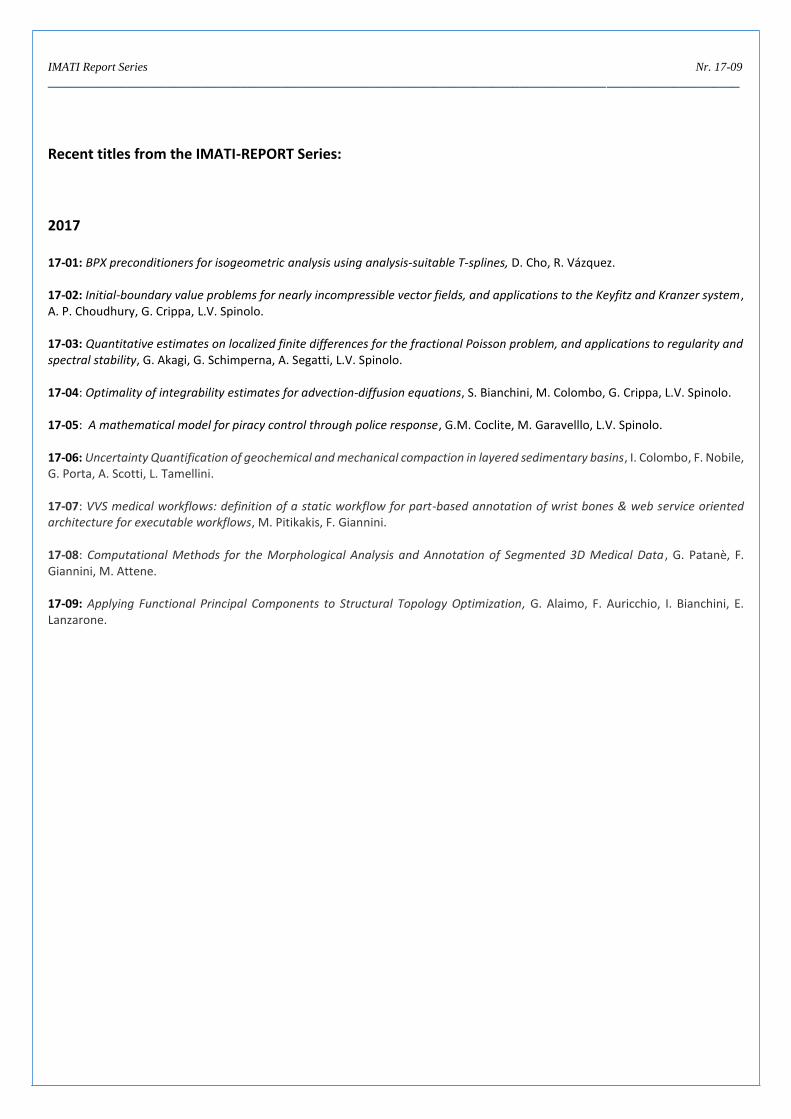
Recent titles from the IMATI-REPORT Series:
2017 17-01: BPX preconditioners for isogeometric analysis using analysis-suitable T-splines, D. Cho, R. Vázquez. 17-02: Initial-boundary value problems for nearly incompressible vector fields, and applications to the Keyfitz and Kranzer system, A. P. Choudhury, G. Crippa, L.V. Spinolo. 17-03: Quantitative estimates on localized finite differences for the fractional Poisson problem, and applications to regularity and spectral stability, G. Akagi, G. Schimperna, A. Segatti, L.V. Spinolo. 17-04: Optimality of integrability estimates for advection-diffusion equations, S. Bianchini, M. Colombo, G. Crippa, L.V. Spinolo. 17-05: A mathematical model for piracy control through police response, G.M. Coclite, M. Garavelllo, L.V. Spinolo. 17-06: Uncertainty Quantification of geochemical and mechanical compaction in layered sedimentary basins, I. Colombo, F. Nobile, G. Porta, A. Scotti, L. Tamellini. 17-07: VVS medical workflows: definition of a static workflow for part-based annotation of wrist bones & web service oriented architecture for executable workflows, M. Pitikakis, F. Giannini. 17-08: Computational Methods for the Morphological Analysis and Annotation of Segmented 3D Medical Data , G. Patanè, F. Giannini, M. Attene. 17-09: Applying Functional Principal Components to Structural Topology Optimization, G. Alaimo, F. Auricchio, I. Bianchini, E. Lanzarone.